1
Parallel Programming Using the Global Arrays
Toolkit
Bruce Palmer, Sriram Krishnamoorthy, Daniel
Chavarria, Abhinav Vishnu, Jeff Daily,
Pacific Northwest National Laboratory
Global Arrays
! Developed over 20 years
! Under active development and focusing on preparing for
future exascale platforms
! Available across platforms from PCs to leadership
machines
! Easy access to distributed data on multiprocessor
machines
!
High programmer productivity
! Library available from: http://www.emsl.pnl.gov/docs/
global
Outline of the Tutorial
!
!
!
!
!
Overview of parallel programming
Introduction to Global Arrays programming model
Basic GA commands
Advanced features of the GA Toolkit
Current and future developments in GA
Why Parallel?
!
!
!
When to Parallelize:
! Program takes too long to execute on a single processor
! Program requires too much memory to run on a single processor
! Program contains multiple elements that are executed or could be
executed independently of each other
Advantages of parallel programs:
! Single processor performance is not increasing. The only way to
improve performance is to write parallel programs.
! Data and operations can be distributed amongst N processors
instead of 1 processor. Codes execute potentially N times as
quickly.
Disadvantages of parallel programs:
! They are bad for your mental health
Parallel vs Serial
! Parallel codes can divide the work and memory required
for application execution amongst multiple processors
! New costs are introduced into parallel codes:
!
!
!
Communication
Code complexity
New dependencies
Communication
! Parallel applications require data to be communicated
from one processor to another at some point
! Data can be communicated by having processors
exchanging data via messages (message-passing)
! Data can be communicated by having processors directly
write or read data in another processors memory
(onesided)
Data Transfers
! The amount of time required to transfer data consists of
two parts
!
!
Latency: the time to initiate data transfer, independent of
data size
Transfer time: the time to actually transfer data once the
transfer is started, proportional to data size
Latency
Data Transfer
Because of latency costs, a single large message
is preferred over many small messages
Parallel Efficiency
Strong Scaling:
For a given size problem, the time to execute is inversely proportional
to the number of processors used. If you want to get your answers
faster, you want a strong scaling program.
! Weak Scaling:
If the problem size increases in proportion to the number of
processors, the execution time is constant. If you want to run larger
calculations, you are looking for weak scaling.
! Speedup:
The ratio of the execution time on N processors to the execution time
on 1 processor. If your code is linearly scaling (the best case) then
speedup is equal to the number of processors.
! Strong Scaling and Weak Scaling are not incompatible. You can have
both.
!
Sources of Parallel Inefficiency
!
!
Communication
! Message latency is a constant regardless of number of
processors
! Not all message sizes decrease with increasing numbers of
processors
! Number of messages per processor may increase with number of
processors, particularly for global operations such as
synchronizations, etc.
Load Imbalance
! Some processors are assigned more work than others resulting in
processors that are idle
Note: parallel inefficiency is like death and taxes. It’s inevitable. The
goal of parallel code development is to put off as long as possible the
point at which the inefficiencies dominate.
Increasing Scalability
!
!
!
Design algorithms to minimize communication
! Exploit data locality
! Aggregate messages
Overlapping computation and communication
! On most high end platforms, computation and communication use
non-overlapping resources. Communication can occur
simultaneously with computation
! Onesided non-blocking communication and double buffering
Load balancing
! Static load balancing: partition calculation at startup so that each
processor has approximately equal work
! Dynamic load balancing: structure algorithm to repartition work
while calculation is running. Note that dynamic load balancing
generally increases the other source of parallel inefficiency,
communication.
Outline of the Tutorial
!
!
!
!
!
Overview of parallel programming
Introduction to Global Arrays programming model
Basic GA commands
Advanced features of the GA Toolkit
Current and future developments in GA
Distributed Data vs Shared Memory
Shared Memory:
Data is in a globally accessible address space, any processor
can access data by specifying its location using a global
index
Data is mapped out in
a natural manner
(usually
corresponding to the
original problem) and
access is easy.
Information on data
locality is obscured
and leads to loss of
performance.
(1,1)
(47,95)
(106,171)
(150,200)
Distributed vs Shared Data View
Distributed Data:
Data is explicitly associated with each processor, accessing
data requires specifying the location of the data on the
processor and the processor itself.
Data locality is explicit
but data access is
complicated.
Distributed computing
is typically
implemented with
message passing
(e.g. MPI)
(0xf5670,P0)
(0xf32674,P5)
P0
P1
P2
Global Arrays
Distributed dense arrays that can be accessed through a
shared memory-like style
Physically distributed data
single, shared data structure/
global indexing
e.g., access A(4,3) rather than
buf(7) on task 2
Global Address Space
Creating Global Arrays
integer array
handle
character string
minimum block size
on each processor
g_a = NGA_Create(type, ndim, dims, name, chunk)
float, double, int, etc.
array of dimensions
dimension
One-sided Communication
Message Passing:
receive
send
P1
P0
message passing
MPI
Message requires cooperation
on both sides. The processor
sending the message (P1) and
the processor receiving the
message (P0) must both
participate.
One-sided Communication:
P0
put
P1
one-sided communication
SHMEM, ARMCI, MPI-2-1S
Once message is initiated on
sending processor (P1) the
sending processor can
continue computation.
Receiving processor (P0) is
not involved. Data is copied
directly from switch into
memory on P0.
Remote Data Access in GA vs MPI
Message Passing:
copy local data on P0 to local buffer
Global Array Global upper
handle
and lower
indices of data
patch
}
loop over processors:
if (me = P_N) then
pack data in local message
buffer
send block of data to
message buffer on P0
else if (me = P0) then
receive block of data from
P_N in message buffer
unpack data from message
buffer to local buffer
endif
end loop
NGA_Get(g_a, lo, hi, buffer, ld);
}
identify size and location of data
blocks
Global Arrays:
Local buffer
and array of
strides
P0
P2
P1
P3
Onesided vs Message Passing
! Message-passing
!
!
!
Communication patterns are regular or at least predictable
Algorithms have a high degree of synchronization
Data consistency is straightforward
! One-sided
!
Communication is irregular
!
!
Algorithms are asynchronous
!
!
Load balancing
But also can be used for synchronous algorithms
Data consistency must be explicitly managed
GLOBAL ARRAY MODEL OF COMPUTATIONS
Shared Object
compute/update
local memory
to sh
copy
emory
local m
put
get
local memory
ared
o
copy to
bjec
t
Shared Object
local memory
Global Arrays vs. Other Models
Advantages:
! Inter-operates with MPI
!
Use more convenient global-shared view for multidimensional arrays, but can use MPI model wherever needed
! Data-locality and granularity control is explicit with GA’s
get-compute-put model, unlike the non-transparent
communication overheads with other models (except MPI)
! Library-based approach: does not rely upon smart compiler
optimizations to achieve high performance
Disadvantage:
! Data consistency must be explicitly managed
Global Arrays (cont.)
!
!
!
!
!
!
!
Shared data model in context of distributed dense arrays
Much simpler than message-passing for many
applications
Complete environment for parallel code development
Compatible with MPI
Data locality control similar to distributed memory/
message passing model
Extensible
Scalable
Data Locality in GA
What data does a processor own?
NGA_Distribution(g_a, iproc, lo, hi);
Where is the data?
NGA_Access(g_a, lo, hi, ptr, ld)
Use this information to organize calculation so that
maximum use is made of locally held data
Example: Matrix Multiply
=
nga_put!
•
nga_get!
=
•
dgemm!
local buffers on the
processor
global arrays
representing
matrices
Matrix Multiply
(a better version)
more scalable!
=
•
atomic accumulate
get
=
•
dgemm
local buffers on the
processor
(less memory,
higher parallelism)
Application Areas
electronic structure chemistry
bioinformatics
Major area
smoothed particle
hydrodynamics
material sciences
visual analytics
fluid dynamics
hydrology
molecular dynamics
Others: financial security forecasting, astrophysics, biology, climate analysis
Recent Applications
ScalaBLAST
C. Oehmen and J. Nieplocha. ScalaBLAST: "A scalable
implementation of BLAST for high performance dataintensive bioinformatics analysis." IEEE Trans. Parallel
Distributed Systems, Vol. 17, No. 8, 2006
Parallel Inspire
Krishnan M, SJ Bohn, WE Cowley, VL Crow, and J Nieplocha,
"Scalable Visual Analytics of Massive Textual Datasets",
Proc. IEEE International Parallel and Distributed
Processing Symposium, 2007.
Smooth Particle Hydrodynamics
B. Palmer, V. Gurumoorthi, A. Tartakovsky, T. Scheibe, A
Component-Based Framework for Smoothed Particle
Hydrodynamics Simulations of Reactive Fluid Flow in Portous
Media”, Int. J. High Perf. Comput. App., Vol 24, 2010
Recent Applications
Subsurface Transport Over
Multiple Phases: STOMP
Transient Energy Transport
Hydrodynamics Simulator:
TETHYS
Outline of the Tutorial
!
!
!
!
!
Overview of parallel programming
Introduction to Global Arrays programming model
Basic GA commands
Advanced features of the GA Toolkit
Current and future developments in GA
Structure of GA
Application
programming
language interface
Global Arrays
and MPI are
completely
interoperable.
Code can
contain calls
to both
libraries.
Fortran
C
C++
Python
distributed arrays layer
memory management, index translation
MPI
Global
operations
ARMCI
portable 1-sided communication
put, get, locks, etc
system specific interfaces
LAPI, Infiniband, threads, VIA,..
Writing GA Programs
! GA requires the following
functionalities from a message
passing library (MPI/TCGMSG)
!
!
!
initialization and termination of
processes
Broadcast, Barrier
a function to abort the running
parallel job in case of an error
#include
#include
#include
#include
int main( int argc, char **argv ) {
MPI_Init( &argc, &argv );
GA_Initialize();
printf( "Hello world\n" );
GA_Terminate();
MPI_Finalize();
return 0;
}
! The message-passing library has to
be
!
!
initialized before the GA library
terminated after the GA library is
terminated
! GA is compatible with MPI
<stdio.h>
"mpi.h"
"ga.h"
"macdecls.h"
Source Code and More
Information
! Version 5.0.2 available
! Homepage at http://www.emsl.pnl.gov/docs/global/
! Platforms
!
!
!
!
!
!
!
!
!
IBM SP, BlueGene
Cray XT, XE6 (Gemini)
Linux Cluster with Ethernet, Infiniband
Solaris
Fujitsu
Hitachi
NEC
HP
Windows
Documentation on Writing, Building and
Running GA programs
!
For detailed information
! GA Webpage
! GA papers, APIs, user manual, etc.
! (Google: Global Arrays)
! http://www.emsl.pnl.gov/docs/global/
! GA User Manual
! http://www.emsl.pnl.gov/docs/global/user.html
! GA API Documentation
! GA Webpage => User Interface
! http://www.emsl.pnl.gov/docs/global/
userinterface.html
! GA Support/Help
! [email protected] or [email protected]
! 2 mailing lists: GA User Forum, and GA Announce
Installing GA
!
!
GA 5.0 established autotools (configure && make && make install) for building
! No environment variables are required
!
Traditional configure env vars CC, CFLAGS, CPPFLAGS, LIBS, etc
! Specify the underlying network communication protocol
!
Only required on clusters with a high performance network
! e.g. If the underlying network is Infiniband using OpenIB protocol use:
configure --with-openib
! GA requires MPI for basic start-up and process management
!
You can either use MPI or TCGMSG wrapper to MPI
! MPI is the default: configure
! TCGMSG-MPI wrapper: configure --with-mpi --with-tcgmsg
! TCGMSG: configure --with-tcgmsg
Various “make” targets
!
!
!
!
!
“make” to build GA libraries
“make install” to install libraries
“make checkprogs” to build tests and examples
“make check MPIEXEC=‘mpiexec -np 4’” to run test suite
VPATH builds: one source tree, many build trees i.e. configurations
Compiling and Linking GA Programs
Your Makefile: Please refer to the CFLAGS, FFLAGS, CPPFLAGS, LDFLAGS
and LIBS variables, which will be printed if you “make flags”.
# ===========================================================================
# Suggested compiler/linker options are as follows.
# GA libraries are installed in /Users/d3n000/ga/ga-5-0/bld_openmpi_shared/lib
# GA headers are installed in /Users/d3n000/ga/ga-5-0/bld_openmpi_shared/include
#
CPPFLAGS="-I/Users/d3n000/ga/ga-5-0/bld_openmpi_shared/include"
#
LDFLAGS="-L/Users/d3n000/ga/ga-5-0/bld_openmpi_shared/lib"
#
# For Fortran Programs:
FFLAGS="-fdefault-integer-8"
LIBS="-lga -framework Accelerate"
#
# For C Programs:
CFLAGS=""
LIBS="-lga -framework Accelerate -L/usr/local/lib/gcc/x86_64-apple-darwin10/4.6.0
-L/usr/local/lib/gcc/x86_64-apple-darwin10/4.6.0/../../.. -lgfortran"
# ===========================================================================
You can use these variables in your Makefile:
For example: gcc $(CPPLAGS) $(LDFLAGS) -o ga_test ga_test.c $(LIBS)
Writing GA Programs
! GA Definitions and Data types
!
!
C programs include files: ga.h, macdecls.h
Fortran programs should include the files: mafdecls.fh,
global.fh.
#include
#include
#include
#include
<stdio.h>
"mpi.h“
"ga.h"
"macdecls.h"
int main( int argc, char **argv ) {
/* Parallel program */
}
Running GA Programs
! Example: Running a test program “ga_test” on 2 processes
for GA built using the MPI runtime
! mpirun -np 2 ga_test
! Running a GA program is same as MPI
11 Basic GA Operations
! GA programming model is very simple.
! Most of a parallel program can be written with
these basic calls
!
!
!
!
!
!
GA_Initialize, GA_Terminate
GA_Nnodes, GA_Nodeid
GA_Create, GA_Destroy
GA_Put, GA_Get
GA Distribution, GA_Access
GA_Sync
GA Initialization/Termination
program main
#include “mafdecls.fh”
!
!
#include “global.fh”
integer ierr
There are two functions to initialize GA:
c
! Fortran
call mpi_init(ierr)
call ga_initialize()
! subroutine ga_initialize()
c
! subroutine ga_initialize_ltd(limit)
write(6,*) ‘Hello world’
c
! C
call ga_terminate()
call mpi_finalize()
! void GA_Initialize()
end
! void GA_Initialize_ltd(size_t limit)
! Python
! import ga, then ga.set_memory_limit(limit)
To terminate a GA program:
! Fortran subroutine ga_terminate()
! C
void GA_Terminate()
! Python N/A
Parallel Environment - Process Information
! Parallel Environment:
!
!
how many processes are working together (size)
what their IDs are (ranges from 0 to size-1)
! To return the process ID of the current process:
!
!
!
Fortran integer function ga_nodeid()
C
int GA_Nodeid()
Python nodeid = ga.nodeid()
! To determine the number of computing processes:
!
!
!
Fortran integer function ga_nnodes()
C
int GA_Nnodes()
Python nnodes = ga.nnodes()
Parallel Environment - Process Information
(EXAMPLE)
$ mpirun –np 4 helloworld
program main
#include “mafdecls.fh”
#include “global.fh”
integer ierr,me,nproc
call mpi_init(ierr)
call ga_initialize()
Hello
Hello
Hello
Hello
world:
world:
world:
world:
My
My
My
My
rank
rank
rank
rank
is
is
is
is
0
2
3
1
out
out
out
out
of
of
of
of
40
processes/nodes
processes/nodes
processes/nodes
processes/nodes
$ mpirun –np 4 python helloworld.py
Hello world: My rank is 0 out of 4 processes/nodes
Hello world: My rank is 2 out of 4 processes/nodes
Hello world: My rank is 3 out of 4 processes/nodes
Hello world: My rank is 1 out of 4 processes/nodes
me = ga_nodeid()
size = ga_nnodes()
write(6,*) ‘Hello world: My rank is ’ + me + ‘ out of ‘ +
&
size + ‘processes/nodes’
call ga_terminate()
call mpi_finilize()
end
4
4
4
4
GA Data Types
!
!
C Data types
! C_INT
! C_LONG
! C_FLOAT
! C_DBL
! C_SCPL
! C_DCPL
Fortran Data types
! MT_F_INT
! MT_F_REAL
! MT_F_DBL
! MT_F_SCPL
! MT_F_DCPL
- int
- long
- float
- double
- single complex
- double complex
- integer (4/8 bytes)
- real
- double precision
- single complex
- double complex
Creating/Destroying Arrays
!
To create an array with a regular distribution:
! Fortran logical function nga_create(type, ndim, dims, name,
chunk, g_a)
! C
int NGA_Create(int type, int ndim, int dims[],
char *name, int chunk[])
! Python g_a = ga.create(type, dims, name="", chunk=None,
int pgroup=-1)
character*(*)
integer
integer
integer
name
type
dims()
chunk()
integer
g_a
- a unique character string
- GA data type
- array dimensions
- minimum size that dimensions
should be chunked into
- array handle for future references
[input]
[input]
[input]
[input]
[output]
dims(1) = 5000
dims(2) = 5000
chunk(1) = -1
!Use defaults
chunk(2) = -1
if (.not.nga_create(MT_F_DBL,2,dims,’Array_A’,chunk,g_a))
+
call ga_error(“Could not create global array A”,g_a)
Creating/Destroying Arrays (cont.)
! To create an array with an irregular distribution:
!
!
!
Fortran logical function nga_create_irreg (type, ndim,
dims, array_name, map, nblock, g_a)
C
int NGA_Create_irreg(int type, int ndim, int dims[],
char* array_name, nblock[], map[])
Python g_a = ga.create_irreg(int gtype, dims, block, map,
name="", pgroup=-1)
character*(*)
integer
integer
integer
integer
integer
name
type
dims
nblock(*)
map(*)
g_a
- a unique character string
[input]
- GA datatype
[input]
- array dimensions
[input]
- no. of blocks each dimension is divided into [input]
- starting index for each block
[input]
- integer handle for future references
[output]
Creating/Destroying Arrays (cont.)
!
Example of irregular distribution:
! The distribution is specified as a Cartesian product of distributions for
each dimension. The array indices start at 1.
! The figure demonstrates distribution of a 2-dimensional array 8x10 on
6 (or more) processors. block[2]={3,2}, the size of map array is s=5
and array map contains the following elements map={1,3,7, 1, 6}.
! The distribution is nonuniform because, P1 and P4 get 20 elements
each and processors P0,P2,P3, and P5 only 10 elements each.
block(1) = 3
block(2) = 2
map(1) = 1
map(2) = 3
map(3) = 7
map(4) = 1
map(5) = 6
if (.not.nga_create_irreg(MT_F_DBL,2,dims, &
’Array_A’,map,block,g_a)) &
call ga_error(“Could not create array A”,g_a)
5
5
P0
P3
2
P1
P4
4
P2
P5
2
Creating/Destroying Arrays (cont.)
! To duplicate an array:
!
!
!
Fortran logical function ga_duplicate(g_a, g_b, name)
C
int GA_Duplicate(int g_a, char *name)
Python ga.duplicate(g_a, name)
! Global arrays can be destroyed by calling the function:
!
!
!
Fortran subroutine ga_destroy(g_a)
C
void GA_Destroy(int g_a)
Python ga.destroy(g_a)
call
integer
character*(*)
name
g_a
g_b
g_a, g_b;
name;
- a character string
- Integer handle for reference array
- Integer handle for new array
[input]
[input]
[output]
nga_create(MT_F_INT,dim,dims,
+
‘array_a’,chunk,g_a)
call ga_duplicate(g_a,g_b,‘array_b’)
call ga_destroy(g_a)
Put/Get
!
!
Put copies data from a local array to a global array section:
! Fortran subroutine nga_put(g_a, lo, hi, buf, ld)
! C
void NGA_Put(int g_a, int lo[], int hi[], void *buf, int ld[])
! Python ga.put(g_a, buf, lo=None, hi=None)
Get copies data from a global array section to a local array:
! Fortran subroutine nga_get(g_a, lo, hi, buf, ld)
! C
void NGA_Get(int g_a, int lo[], int hi[], void *buf, int ld[])
! Python buffer = ga.get(g_a, lo, hi, numpy.ndarray buffer=None)
integer
integer
Double precision/complex/integer
integer
g_a
lo(),hi()
buf
ld()
global array handle
limits on data block to be moved
local buffer
array of strides for local buffer
[input]
[input]
[output]
[input]
Put/Get (cont.)
! Example of put operation:
!
transfer data from a local buffer (10 x10 array) to (7:15,1:8)
section of a 2-dimensional 15 x10 global array into lo={7,1},
hi={15,8}, ld={10}
global
double precision buf(10,10)
:
:
call nga_put(g_a,lo,hi,buf,ld)
lo
local
hi
Atomic Accumulate
!
Accumulate combines the data from the local array
with data in the global array section:
! Fortran
subroutine nga_acc(g_a, lo, hi,
buf, ld, alpha)
! C
void NGA_Acc(int g_a, int lo[],
int hi[], void *buf, int ld[], void *alpha)
! Python
ga.acc(g_a, buffer, lo=None, hi=None,
alpha=None)
integer
integer
double
integer
double
g_a array handle
lo(), hi() limits on data block to be moved
precision/complex buf local buffer
ld() array of strides for local buffer
precision/complex alpha arbitrary scale factor
[input]
[input]
[input]
[input]
[input]
Atomic Accumulate (cont)
global
local
ga(i,j) = ga(i,j)+alpha*buf(k,l)
Sync
! Sync is a collective operation
! It acts as a barrier, which synchronizes all the processes
and ensures that all outstanding Global Array operations
are complete at the call
! The functions are:
!
!
!
Fortran subroutine ga_sync()
C
void GA_Sync()
Python ga.sync()
GA_sync is the main
mechanism in GA for
guaranteeing data
consistency
sync
Global Operations
! Fortran
subroutine ga_brdcst(type, buf, lenbuf, root)
subroutine ga_igop(type, x, n, op)
subroutine ga_dgop(type, x, n, op)
! C
! Python
void GA_Brdcst(void *buf, int lenbuf, int root)
void GA_Igop(long x[], int n, char *op)
void GA_Dgop(double x[], int n, char *op)
buffer = ga.brdcst(buffer, root)
buffer = ga.gop(x, op)
GLOBAL ARRAY MODEL OF COMPUTATIONS
Shared Object
compute/update
local memory
to sh
copy
emory
local m
put
get
local memory
ared
o
copy to
bjec
t
Shared Object
local memory
Locality Information
!
Discover array elements held by each processor
! Fortran nga_distribution(g_a,proc,lo,hi)
! C
void NGA_Distribution(int g_a, int proc, int *lo, int *hi)
! Python lo,hi = ga.distribution(g_a, proc=-1)
integer
integer
integer
integer
g_a
proc
lo(ndim)
hi(ndim)
array handle
processor ID
lower index
upper index
[input]
[input]
[output]
[output]
do iproc = 1, nproc
write(6,*) ‘Printing g_a info for processor’,iproc
call nga_distribution(g_a,iproc,lo,hi)
do j = 1, ndim
write(6,*) j,lo(j),hi(j)
end do
dnd do
Example: Matrix Multiply
/* Determine which block of data is locally owned. Note that
the same block is locally owned for all GAs. */
NGA_Distribution(g_c, me, lo, hi);
/* Get the blocks from g_a and g_b needed to compute this block in
g_c and copy them into the local buffers a and b. */
lo2[0] = lo[0]; lo2[1] = 0; hi2[0] = hi[0]; hi2[1] = dims[0]-1;
NGA_Get(g_a, lo2, hi2, a, ld);
lo3[0] = 0; lo3[1] = lo[1]; hi3[0] = dims[1]-1; hi3[1] = hi[1];
NGA_Get(g_b, lo3, hi3, b, ld);
/* Do local matrix multiplication and store the result in local
buffer c. Start by evaluating the transpose of b. */
for(i=0; i < hi3[0]-lo3[0]+1; i++)
for(j=0; j < hi3[1]-lo3[1]+1; j++)
btrns[j][i] = b[i][j];
/* Multiply a and b to get c */
for(i=0; i < hi[0] - lo[0] + 1; i++) {
for(j=0; j < hi[1] - lo[1] + 1; j++) {
c[i][j] = 0.0;
nga_put!
for(k=0; k<dims[0]; k++)
c[i][j] = c[i][j] + a[i][k]*btrns[j][k];
}
}
/* Copy c back to g_c */
NGA_Put(g_c, lo, hi, c, ld);
=
•
nga_get!
=
dgemm!
•
New Interface for Creating Arrays
! Developed to handle the proliferating number of properties
that can be assigned to Global Arrays
Fortran
integer function ga_create_handle()
subroutine ga_set_data(g_a, dim, dims, type)
subroutine ga_set_array_name(g_a, name)
subroutine ga_set_chunk(g_a, chunk)
subroutine ga_set_irreg_distr(g_a, map, nblock)
subroutine ga_set_ghosts(g_a, width)
subroutine ga_set_block_cyclic(g_a, dims)
subroutine ga_set_block_cyclic_proc_grid(g_a,
dims, proc_grid)
logical function ga_allocate(g_a)
New Interface for Creating Arrays
C int GA_Create_handle()
void GA_Set_data(int g_a, int dim, int *dims,
int type)
void GA_Set_array_name(int g_a, char* name)
void GA_Set_chunk(int g_a, int *chunk)
void GA_Set_irreg_distr(int g_a, int *map,
int *nblock)
void GA_Set_ghosts(int g_a, int *width)
void GA_Set_block_cyclic(int g_a, int *dims)
void GA_Set_block_cyclic_proc_grid(int g_a, int
*dims,
int *proc_grid)
int GA_Allocate(int g_a)
New Interface for Creating Arrays
Python
handle = ga.create_handle()
ga.set_data(g_a, dims, type)
ga.set_array_name(g_a, name)
ga.set_chunk(g_a, chunk)
ga.set_irreg_distr (g_a, map, nblock)
ga.set_ghosts(g_a, width)
ga.set_block_cyclic(g_a, dims)
ga.set_block_cyclic_proc_grid(g_a, dims,
proc_grid)
bool ga.allocate(int g_a)
New Interface for Creating Arrays (Cont.)
integer ndim,dims(2),chunk(2)
integer g_a, g_b
logical status
c
ndim = 2
dims(1) = 5000
dims(2) = 5000
chunk(1) = 100
chunk(2) = 100
c
c Create global array A using old interface
c
status = nga_create(MT_F_DBL, ndim, dims, chunk, ‘array_A’, g_a)
c
c Create global array B using new interface
C
g_b = ga_create_handle()
call ga_set_data(g_b, ndim, dims, MT_F_DBL)
call ga_set_chunk(g_b, chunk)
call ga_set_name(g_b, ‘array_B’)
call ga_allocate(g_b)
Basic Array Operations
! Whole Arrays:
!
To set all the elements in the array to zero:
!
!
!
!
subroutine ga_zero(g_a)
void GA_Zero(int g_a)
ga.zero(g_a)
To assign a single value to all the elements in array:
!
!
!
!
Fortran
C
Python
Fortran
C
Python
subroutine ga_fill(g_a, val)
void GA_Fill(int g_a, void *val)
ga.fill(g_a, val)
To scale all the elements in the array by factorval:
!
!
!
Fortran
C
Python
subroutine ga_scale(g_a, val)
void GA_Scale(int g_a, void *val)
ga.scale(g_a, val)
Basic Array Operations (cont.)
Whole Arrays:
! To copy data between two arrays:
! Fortran
subroutine ga_copy(g_a, g_b)
! C
void GA_Copy(int g_a, int g_b)
! Python
ga.copy(g_a, g_b)
! Arrays must be same size and dimension
! Distribution may be different
!
“g_a”
“g_b”
0
1
2
3
4
5
6
7
8
0
1
2
3
4
5
6
7
8
call ga_create(MT_F_INT,ndim,dims,
‘array_A’,chunk_a,g_a)
call nga_create(MT_F_INT,ndim,dims,
‘array_B’,chunk_b,g_b)
... Initialize g_a ....
call ga_copy(g_a, g_b)
Global Arrays g_a and g_b distributed on a 3x3 process grid
Basic Array Patch Operations
!
Patch Operations:
! The copy patch operation:
! Fortran
subroutine nga_copy_patch(trans, g_a, alo, ahi,
g_b, blo, bhi)
! C
void NGA_Copy_patch(char trans, int g_a,
int alo[], int ahi[], int g_b, int blo[], int bhi[])
! Python
ga.copy(g_a, g_b, alo=None, ahi=None,
blo=None, bhi=None, bint trans=False)
! Number of elements must match
“g_a”
“g_b”
0
1
2
3
4
5
6
7
8
0
1
2
3
4
5
6
7
8
Basic Array Patch Operations (cont.)
! Patches (Cont):
!
To set only the region defined by lo and hi to zero:
!
!
!
!
Fortran
C
Python
subroutine nga_zero_patch(g_a, lo, hi)
void NGA_Zero_patch(int g_a, int lo[] int hi[])
ga.zero(g_a, lo=None, hi=None)
To assign a single value to all the elements in a patch:
!
!
!
Fortran
C
Python
subroutine nga_fill_patch(g_a, lo, hi, val)
void NGA_Fill_patch(int g_a, int lo[], int hi[], void *val)
ga.fill(g_a, value, lo=None, hi=None)
Basic Array Patch Operations (cont.)
! Patches (Cont):
!
To scale the patch defined by lo and hi by the factor val:
!
Fortran
C
!
Python
!
!
subroutine nga_scale_patch(g_a, lo, hi, val)
void NGA_Scale_patch(int g_a, int lo[], int hi[],
void *val)
ga.scale(g_a, value, lo=None, hi=None)
The copy patch operation:
!
Fortran
!
C
!
Python
subroutine nga_copy_patch(trans, g_a, alo, ahi,
g_b, blo, bhi)
void NGA_Copy_patch(char trans, int g_a,
int alo[], int ahi[], int g_b, int blo[], int bhi[])
ga.copy(g_a, g_b, alo=None, ahi=None,
blo=None, bhi=None, bint trans=False)
Outline of the Tutorial
!
!
!
!
!
Overview of parallel programming
Introduction to Global Arrays programming model
Basic GA commands
Advanced features of the GA Toolkit
Current and future developments in GA
Scatter/Gather
!
!
Scatter puts array elements into a global array:
! Fortran subroutine nga_scatter(g_a, v, subscrpt_array, n)
! C
void NGA_Scatter(int g_a, void *v, int *subscrpt_array[],
int n)
! Python ga.scatter(g_a, values, subsarray)
Gather gets the array elements from a global array into a local array:
! Fortran subroutine nga_gather(g_a, v, subscrpt_array, n)
! C
void NGA_Gather(int g_a, void *v, int *subscrpt_array[],
int n)
! Python values = ga.gather(g_a, subsarray, numpy.ndarray
values=None)
integer
double precision
integer
integer
g_a array handle
v(n) array of values
n number of values
subscrpt_array location of values in global array
[input]
[input/output]
[input]
[input]
Scatter/Gather (cont.)
!
Example of scatter operation:
! Scatter the 5 elements into a 10x10 global array
! Element 1 v[0] = 5
subsArray[0][0] = 2
subsArray[0][1] = 3
! Element 2 v[1] = 3
subsArray[1][0] = 3
subsArray[1][1] = 4
! Element 3 v[2] = 8
subsArray[2][0] = 8
subsArray[2][1] = 5
! Element 4 v[3] = 7
subsArray[3][0] = 3
subsArray[3][1] = 7
! Element 5 v[4] = 2
subsArray[4][0] = 6
subsArray[4][1] = 3
! After the scatter operation, the five elements
would be scattered into the global array as shown
in the figure.
0
0
1
2
3
4
5
6
7
8
9
1
2
3
4
5
6
7
5
3
7
2
8
integer subscript(ndim,nlen)
:
call nga_scatter(g_a,v,subscript,nlen)
8
9
Read and Increment
!
Read_inc remotely updates a particular element in an integer
global array and returns the original value:
! Fortran integer function nga_read_inc(g_a, subscript, inc)
! C
long NGA_Read_inc(int g_a, int subscript[], long inc)
! Python val = ga.read_inc(g_a, subscript, inc=1)
! Applies to integer arrays only
! Can be used as a global counter for dynamic load balancing
integer
integer
g_a
subscript(ndim), inc
[input]
[input]
Read and Increment (cont.)
c
Create task counter
status = nga_create(MT_F_INT,one,one,chunk,g_counter)
call ga_zero(g_counter)
:
itask = nga_read_inc(g_counter,one,one)
... Translate itask into task ...
NGA_Read_inc
(Read and Increment)
Global Array
Global Lock
(access to data
is serialized)
Every integer value is read
once and only once by
some processor
Hartree-Fock SCF
Obtain variational solutions to the electronic
Schrödinger equation
within the approximation of a single Slater determinant.
Assuming the one electron orbitals are expanded as
the calculation reduces to the self-consistent eigenvalue
problem
Parallelizing the Fock Matrix
The bulk of the work involves computing the 4-index elements
(μν|ωλ). This is done by decomposing the quadruple loop
into evenly sized blocks and assigning blocks to each
processor using a global counter. After each processor
completes a block it increments the counter to get the next
block
467
Read and
increment
counter
do i
do j
do k
Accumulate
do l
results
F(i,j)=..
Evaluate
block
Gorden Bell finalist at SC09 - GA Crosses the
Petaflop Barrier
!
GA-based parallel
implementation of coupled
cluster calculation
performed at 1.39
petaflops using over
223,000 processes on
ORNL's Jaguar petaflop
system
!
!
Apra et. al., “Liquid
water: obtaining the right
answer for the right
reasons”, SC 2009.
Global Arrays is one of
two programming models
that have achieved this
level of performance
Direct Access to Local Data
! Global Arrays support abstraction of a distributed array
object
! Object is represented by an integer handle
! A process can access its portion of the data in the
global array
! To do this, the following steps need to be taken:
!
!
!
!
Find the distribution of an array, i.e. which part of the
data the calling process owns
Access the data
Operate on the data: read/write
0
Release the access to the data
3
1
4
Access
!
To provide direct access to local data in the specified patch of the
array owned by the calling process:
! Fortran subroutine nga_access(g_a, lo, hi, index, ld)
! C
void NGA_Access(int g_a, int lo[], int hi[],
void *ptr, int ld[])
! Python ndarray = ga.access(g_a, lo=None, hi=None)
! Processes can access the local position of the global array
! Process “0” can access the specified patch of its local position
of the array
! Avoids memory copy
Access (cont.)
status = nga_create(MT_F_DBL,2,dims,’Array’,chunk,g_a)
:
call nga_distribution(g_a,me,lo,hi)
call nga_access(g_a,lo,hi,index,ld)
call do_subroutine_task(dbl_mb(index),ld(1))
call nga_release(g_a,lo,hi)
subroutine do_subroutine_task(a,ld1)
double precision a(ld1,*)
Access:
gives a
pointer to this
local patch
0
1
2
3
4
5
6
7
8
Non-blocking Operations
!
The non-blocking APIs are derived from the blocking interface by
adding a handle argument that identifies an instance of the nonblocking request.
!
Fortran
!
!
!
!
!
C
!
!
!
!
!
subroutine nga_nbput(g_a, lo, hi, buf, ld, nbhandle)
subroutine nga_nbget(g_a, lo, hi, buf, ld, nbhandle)
subroutine nga_nbacc(g_a, lo, hi, buf, ld, alpha, nbhandle)
subroutine nga_nbwait(nbhandle)
void NGA_NbPut(int g_a, int lo[], int hi[], void *buf, int ld[], ga_nbhdl_t* nbhandle)
void NGA_NbGet(int g_a, int lo[], int hi[], void *buf, int ld[], ga_nbhdl_t* nbhandle)
void NGA_NbAcc(int g_a, int lo[], int hi[], void *buf, int ld[], void *alpha,
ga_nbhdl_t* nbhandle)
int NGA_NbWait(ga_nbhdl_t* nbhandle)
Python
!
!
!
!
handle = ga.nbput(g_a, buffer, lo=None, hi=None)
buffer,handle = ga.nbget(g_a, lo=None, hi=None, numpy.ndarray buffer=None)
handle = ga.nbacc(g_a, buffer, lo=None, hi=None, alpha=None)
ga.nbwait(handle)
Non-Blocking Operations
double precision buf1(nmax,nmax)
double precision buf2(nmax,nmax)
:
call nga_nbget(g_a,lo1,hi1,buf1,ld1,nb1)
ncount = 1
do while(.....)
if (mod(ncount,2).eq.1) then
... Evaluate lo2, hi2
call nga_nbget(g_a,lo2,hi2,buf2,nb2)
call nga_wait(nb1)
... Do work using data in buf1
else
... Evaluate lo1, hi1
call nga_nbget(g_a,lo1,hi1,buf1,nb1)
call nga_wait(nb2)
... Do work using data in buf2
endif
ncount = ncount + 1
end do
SRUMMA Matrix Multiplication
Computation
Comm.
(Overlap)
A
C=A.B
B
=
patch matrix multiplication
http://hpc.pnl.gov/projects/srumma/
SRUMMA Matrix Multiplication:
Improvement over PBLAS/ScaLAPACK
Parallel Matrix Multiplication on the HP/Quadrics Cluster at PNNL
Matrix size: 40000x40000
Efficiency 92.9% w.r t. serial algorithm and 88.2% w.r.t. machine peak on 1849 CPUs
SRUMMA
12
PBLAS/ScaLAPACK pdgemm
10
Theoretical Peak
Perfect Scaling
TeraFLOPs
8
6
4
2
0
0
512
1024
Processors
1536
2048
Cluster Information
! Example:
! 2 nodes with 4 processors each. Say, there are 7
processes created.
!
!
!
!
ga_cluster_nnodes returns 2
ga_cluster_nodeid returns 0 or 1
ga_cluster_nprocs(inode) returns 4 or 3
ga_cluster_procid(inode,iproc) returns a processor ID
Cluster Information (cont.)
! To return the total number of nodes that the program is running
on:
! Fortran integer function ga_cluster_nnodes()
! C
int GA_Cluster_nnodes()
! Python nnodes = ga.cluster_nnodes()
! To return the node ID of the process:
! Fortran integer function ga_cluster_nodeid()
! C
int GA_Cluster_nodeid()
! Python nodeid = ga.cluster_nodeid()
N0
N1
Cluster Information (cont.)
! To return the number of processors available on node inode:
! Fortran integer function ga_cluster_nprocs(inode)
! C
int GA_Cluster_nprocs(int inode)
! Python nprocs = ga.cluster_nprocs(inode)
! To return the processor ID associated with node inode and the
local processor ID iproc:
! Fortran integer function ga_cluster_procid(inode, iproc)
! C
int GA_Cluster_procid(int inode, int iproc)
! Python procid = ga.cluster_procid(inode, iproc)
0(0) 1(1)
4(0) 5(1)
2(2) 3(3)
6(2) 7(3)
Accessing Processor Memory
Node
SMP Memory
R8
R9
R10
R11
P8
P9
P10
P11
ga_access
Processor Groups
!
!
To create a new processor group:
! Fortran integer function ga_pgroup_create(list, size)
! C
int GA_Pgroup_create(int *list, int size)
! Python pgroup = ga.pgroup_create(list)
To assign a processor groups:
! Fortran logical function nga_create_config(
type, ndim, dims, name, chunk, p_handle, g_a)
! C
int NGA_Create_config(int type, int ndim,
int dims[], char *name, int p_handle, int chunk[])
! Python g_a = ga.create(type, dims, name, chunk, pgroup=-1)
integer
integer
integer
integer
]
g_a
p_handle
list(size)
size
- global array handle
- processor group handle
- list of processor IDs in group
- number of processors in group
[input]
[output]
[input]
[input]
Processor Groups
group A
world group
group B
group C
Processor Groups (cont.)
!
To set the default processor group
!
!
!
!
Fortran
subroutine ga_pgroup_set_default(p_handle)
C void GA_Pgroup_set_default(int p_handle)
Python
ga.pgroup_set_default(p_handle)
To access information about the processor group:
!
!
!
integer
Fortran
!
integer function ga_pgroup_nnodes(p_handle)
!
integer function ga_pgroup_nodeid(p_handle)
C
!
int GA_Pgroup_nnodes(int p_handle)
!
int GA_Pgroup_nodeid(int p_handle)
Python
!
nnodes = ga.pgroup_nnodes(p_handle)
!
nodeid = ga.pgroup_nodeid(p_handle)
p_handle
- processor group handle [input]
Processor Groups (cont.)
! To determine the handle for a standard group at any point
in the program:
!
Fortran
!
!
!
!
C
!
!
!
!
integer function ga_pgroup_get_default()
integer function ga_pgroup_get_mirror()
integer function ga_pgroup_get_world()
int GA_Pgroup_get_default()
int GA_Pgroup_get_mirror()
int GA_Pgroup_get_world() )
Python
!
!
!
p_handle = ga.pgroup_get_default()
p_handle = ga.pgroup_get_mirror()
p_handle = ga.pgroup_get_world()
Default Processor Group
c
c
c
create subgroup p_a
p_a = ga_pgroup_create(list, nproc)
call ga_pgroup_set_default(p_a)
call parallel_task()
call ga_pgroup_set_default(ga_pgroup_get_world())
subroutine parallel_task()
p_b = ga_pgroup_create(new_list, new_nproc)
call ga_pgroup_set_default(p_b)
call parallel_subtask()
MD Application on Groups
Creating Arrays with Ghost Cells
!
To create arrays with ghost cells:
! For arrays with regular distribution:
!
Fortran
logical function nga_create_ghosts(type,
dims, width, array_name, chunk, g_a)
!
C
int int NGA_Create_ghosts(int type,
int ndim, int dims[], int width[],
char *array_name, int chunk[])
!
Python
g_a = ga.create_ghosts(type, dims, width,
name=“”, chunk=None, pgroup=-1)
! For arrays with irregular distribution:
!
n-d Fortran
logical function nga_create_ghosts_irreg(type,
dims, width, array_name, map, block, g_a)
!
C
int NGA_Create_ghosts_irreg(int type,
Code
int ndim, int dims[], int width[],
char *array_name, int map[], int block[])
!
Python
g_a = ga.create_ghosts_irreg(type, dims, width,
block, map, name=“”, pgroup=-1)
integer width(ndim) - array of ghost cell widths [input]
Ghost Cells
normal global array
Operations:
NGA_Create_ghosts
GA_Update_ghosts
NGA_Access_ghosts
elements
NGA_Nbget_ghost_dir
global array with ghost cells
- creates array with ghosts cells
- updates with data from adjacent processors
- provides access to “local” ghost cell
- nonblocking call to update ghosts cells
Ghost Cell Update
Automatically update ghost
cells with appropriate data
from neighboring
processors. A multiprotocol
implementation has been
used to optimize the
update operation to match
platform characteristics.
Periodic Interfaces
! Periodic interfaces to the one-sided operations have been
added to Global Arrays in version 3.1 to support
computational fluid dynamics problems on
multidimensional grids.
! They provide an index translation layer that allows users
to request blocks using put, get, and accumulate
operations that possibly extend beyond the boundaries of
a global array.
! The references that are outside of the boundaries are
wrapped around inside the global array.
! Current version of GA supports three periodic operations:
!
!
!
periodic get
periodic put
periodic acc
Periodic Interfaces
global
ndim = 2
dims(1) = 10
dims(2) = 10
:
lo(1) = 6
lo(2) = 6
hi(1) = 11
hi(2) = 11
call nga_periodic_get(g_a,lo,hi,buf,ld)
local
Periodic Get/Put/Accumulate
!
!
!
Fortran subroutine nga_periodic_get(g_a, lo, hi, buf, ld)
C
void NGA_Periodic_get(int g_a, int lo[], int hi[], void *buf, int ld[])
Python ndarray = ga.periodic_get(g_a, lo=None, hi=None, buffer=None)
!
!
!
Fortran subroutine nga_periodic_put(g_a, lo, hi, buf, ld)
C
void NGA_Periodic_put(int g_a, int lo[], int hi[], void *buf, int ld[])
Python ga.periodic_put(g_a, buffer, lo=None, hi=None)
!
!
Fortran subroutine nga_periodic_acc(g_a, lo, hi, buf, ld, alpha)
C
void NGA_Periodic_acc(int g_a, int lo[], int hi[], void *buf, int ld[],
void *alpha)
Python ga.periodic_acc(g_a, buffer, lo=None, hi=None, alpha=None)
!
Lock and Mutex
! Lock works together with mutex.
! Simple synchronization mechanism to protect a critical
section
! To enter a critical section, typically, one needs to:
!
!
!
!
!
Create mutexes
Lock on a mutex
Do the exclusive operation in the critical section
Unlock the mutex
Destroy mutexes
! The create mutex functions are:
!
!
!
Fortran
C
Python
logical function ga_create_mutexes(number)
int GA_Create_mutexes(int number)
bool ga.create_mutexes(number)
Lock and Mutex (cont.)
Lock
Unlock
Lock and Mutex (cont.)
!
!
The destroy mutex functions are:
! Fortran
logical function ga_destroy_mutexes()
! C
int GA_Destroy_mutexes()
! Python
bool ga.destroy_mutexes()
The lock and unlock functions are:
! Fortran
! subroutine ga_lock(int mutex)
! subroutine ga_unlock(int mutex)
! C
! void GA_lock(int mutex)
! void GA_unlock(int mutex)
! Python
! ga.lock(mutex)
! ga.unlock(mutex)
integer
mutex
[input] ! mutex id
Fence
!
!
!
!
Fence blocks the calling process until all the data transfers corresponding to
the Global Array operations initiated by this process complete
For example, since ga_put might return before the data reaches final
destination, ga_init_fence and ga_fence allow process to wait until the data
transfer is fully completed
! ga_init_fence();
! ga_put(g_a, ...);
! ga_fence();
The initialize fence functions are:
! Fortran
subroutine ga_init_fence()
! C
void GA_Init_fence()
! Python
ga.init_fence()
The fence functions are:
! Fortran
subroutine ga_fence()
! C
void GA_Fence()
! Python
ga.fence()
Synchronization Control in Collective
Operations
!
To eliminate redundant synchronization points:
! Fortran subroutine ga_mask_sync(prior_sync_mask,
post_sync_mask)
! C
void GA_Mask_sync(int prior_sync_mask,
int post_sync_mask)
! Python ga.mask_sync(prior_sync_mask, post_sync_mask)
logical
logical
first
last
- mask (0/1) for prior internal synchronization
- mask (0/1) for post internal synchronization
[input]
[input]
sync
status = ga_duplicate(g_a, g_b)
call ga_mask(0,1)
call ga_zero(g_b)
duplicate
sync
sync
duplicate
sync
sync
zero
sync
zero
sync
Linear Algebra
!
!
To add two arrays:
! Fortran
subroutine ga_add(alpha, g_a, beta, g_b, g_c)
! C
void GA_Add(void *alpha, int g_a, void *beta, int g_b, int g_c)
! Python
ga.add(g_a, g_b, g_c, alpha=None, beta=None,
alo=None, ahi=None, blo=None, bhi=None,
clo=None, chi=None)
To multiply arrays:
! Fortran
subroutine ga_dgemm(transa, transb, m, n, k, alpha, g_a, g_b,
beta, g_c)
! C
void GA_Dgemm(char ta, char tb, int m, int n, int k, double
alpha, int g_a, int g_b, double beta, int g_c)
! Python
def gemm(bool ta, bool tb, m, n, k, alpha, g_a, g_b, beta, g_c)
double precision/complex/integer
integer
character*1
integer
alpha, beta
g_a, g_b, g_c
transa, transb
m, n, k
- scale factor
- array handles
[input]
[input]
[input]
[input]
Linear Algebra (cont.)
! To compute the element-wise dot product of two arrays:
!
Three separate functions for data types
!
Integer
! Fortran
! C
!
Double precision
! Fortran
! C
!
ga_ddot(g_a, g_b)
GA_Ddot(int g_a, int g_b)
Double complex
! Fortran
! C
!
ga_idot(g_a, g_b)
GA_Idot(int g_a, int g_b)
ga_zdot(g_a, g_b)
GA_Zdot(int g_a, int g_b)
Python has only one function: ga_dot(g_a, g_b)
integer
integer
long
float
double
DoubleComplex
g_a, g_b
[input]
GA_Idot(int g_a, int g_b)
GA_Ldot(int g_a, int g_b)
GA_Fdot(int g_a, int g_b)
GA_Ddot(int g_a, int g_b)
GA_Zdot(int g_a, int g_b)
Linear Algebra (cont.)
! To symmetrize a matrix:
!
!
!
Fortran
C
Python
subroutine ga_symmetrize(g_a)
void GA_Symmetrize(int g_a)
ga.symmetrize(g_a)
! To transpose a matrix:
!
!
!
Fortran
C
Python
subroutine ga_transpose(g_a, g_b)
void GA_Transpose(int g_a, int g_b)
ga.transpose(g_a, g_b)
Linear Algebra on Patches
!
To add element-wise two patches and save the results into another
patch:
!
Fortran
subroutine nga_add_patch(alpha, g_a, alo, ahi, beta,
g_b, blo, bhi, g_c, clo, chi)
!
C
void NGA_Add_patch(void *alpha, int g_a, int alo[], int ahi[],
void *beta, int g_b, int blo[], int bhi[], int g_c, int clo[], int chi[])
!
Python
integer
dbl prec/comp/int
integer
integer
integer
ga.add(g_a, g_b, g_c, alpha=None, beta=None,
alo=None, ahi=None, blo=None, bhi=None,
clo=None, chi=None)
g_a, g_b, g_c
alpha, beta
ailo, aihi, ajlo, ajhi
bilo, bihi, bjlo, bjhi
cilo, cihi, cjlo, cjhi
scale factors
g_a patch coord
g_b patch coord
g_c patch coord
[input]
[input]
[input]
[input]
[input]
Linear Algebra on Patches (cont.)
!
To perform matrix multiplication:
! Fortran
subroutine ga_matmul_patch(transa, transb, alpha, beta,
g_a, ailo, aihi, ajlo, ajhi,
g_b, bilo, bihi, bjlo, bjhi,
g_c, cilo, cihi, cjlo, cjhi)
! C
void GA_Matmul_patch(char *transa, char* transb,
void* alpha, void *beta,
int g_a, int ailo, int aihi, int ajlo, int ajhi,
int g_b, int bilo, int bihi, int bjlo, int bjhi,
int g_c, int cilo, int cihi, int cjlo, int cjhi)
! Fortran
subroutine ga_matmul_patch(bool transa, bool transb,
alpha, beta,
g_a, ailo, aihi, ajlo, ajhi,
g_b, bilo, bihi, bjlo, bjhi,
g_c, cilo, cihi, cjlo, cjhi)
integer
integer
integer
dbl prec/comp
character*1
g_a, ailo, aihi, ajlo, ajhi
g_b, bilo, bihi, bjlo, bjhi
g_c, cilo, cihi, cjlo, cjhi
alpha, beta
transa, transb
patch of g_a
patch of g_b
patch of g_c
scale factors
transpose flags
[input]
[input]
[input]
[input]
[input]
Linear Algebra on Patches (cont.)
!
To compute the element-wise dot product of two arrays:
! Three separate functions for data types
!
Integer
! Fortran
nga_idot_patch(g_a, ta, alo, ahi, g_b, tb, blo, bhi)
! C
NGA_Idot_patch(int g_a, char* ta,
int alo[], int ahi[], int g_b, char* tb, int blo[], int bhi[])
!
Double precision
! Fortran
nga_ddot_patch(g_a, ta, alo, ahi, g_b, tb, blo, bhi)
! C
NGA_Ddot_patch(int g_a, char* ta,
int alo[], int ahi[], int g_b, char* tb, int blo[], int bhi[])
!
Double complex
! Fortran
nga_zdot_patch(g_a, ta, alo, ahi, g_b, tb, blo, bhi)
! C
NGA_Zdot_patch(int g_a, char* ta,
int alo[], int ahi[], int g_b, char* tb, int blo[], int bhi[])
! Python has only one function:
ga.dot(g_a, g_b,
alo=None, ahi=None, blo=None, bhi=None, bint ta=False, bint tb=False)
integer
integer
long
float
double
DoubleComplex
g_a, g_b
GA_Idot(int g_a, int g_b)
GA_Ldot(int g_a, int g_b)
GA_Fdot(int g_a, int g_b)
GA_Ddot(int g_a, int g_b)
GA_Zdot(int g_a, int g_b)
[input]
Block-Cyclic Data Distributions
Normal Data Distribution
Block-Cyclic Data Distribution
Block-Cyclic Data (cont.)
Simple Distribution
0 6 12 18 24 30
1 7 13 19 25 31
2 8 14 20 26 32
3 9 15 21 27 33
Scalapack Distribution
0 1 0
0 0,0 0,1
1 1,0 1,1
1 0
1
0
4 10 16 22 28 34
1
0
5 11 17 23 29 35
1
2 x 2 processor grid
Block-Cyclic Data (cont.)
! Most operations work exactly the same, data distribution
is transparent to the user
! Some operations (matrix multiplication, non-blocking put,
get) not implemented
! Additional operations added to provide access to data
associated with particular sub-blocks
! You need to use the new interface for creating Global
Arrays to get create block-cyclic data distributions
Creating Block-Cyclic Arrays
!
Must use new API for creating Global Arrays
! Fortran subroutine ga_set_block_cyclic(g_a, dims)
subroutine ga_set_block_cyclic_proc_grid(g_a, dims,
proc_grid)
! C
void GA_Set_block_cyclic(int g_a, int dims[])
void GA_Set_block_cyclic_proc_grid(g_a, dims[], proc_grid
[])
! Python ga.set_block_cyclic(g_a, dims)
ga.set_block_cyclic_proc_grid(g_a, block, proc_grid)
integer dims[]
integer proc_grid[]
- dimensions of blocks
- dimensions of processor grid (note that product of all proc_grid dimensions
Block-Cyclic Methods
!
Methods for accessing data of individual blocks
! Fortran
subroutine ga_get_block_info(g_a, num_blocks, block_dims)
integer function ga_total_blocks(g_a)
subroutine nga_access_block_segment(g_a, iproc, index, length)
subroutine nga_access_block(g_a, idx, index, ld)
subroutine nga_access_block_grid(g_a, subscript, index, ld)
! C
void GA_Get_block_info(g_a, num_blocks[], block_dims[])
int GA_Total_blocks(int g_a)
void NGA_Access_block_segment(int g_a, int iproc, void *ptr, int
*length)
void NGA_Access_block(int g_a, int idx, void *ptr, int ld[])
void NGA_Access_block_grid(int g_a, int subscript[], void *ptr, int ld[])
! Python
num_blocks,block_dims = ga.get_block_info(g_a)
blocks = ga.total_blocks(g_a)
ndarray = ga.access_block_segment(g_a, iproc)
ndarray = ga.access_block(g_a, idx)
ndarray = ga.access_block_grid(g_a, subscript)
integer length
integer idx
integer subscript[]
- total size of blocks held on processor
- index of block in array (for simple block-cyclic distribution)
- location of block in block grid (for Scalapack distribution)
Interfaces to Third Party Software Packages
! Scalapack
!
!
Solve a system of linear equations
Compute the inverse of a double precision matrix
! TAO
!
General optimization problems
! Interoperability with Others
!
!
PETSc
CUMULVS
Data Mapping Information
!
To determine the process ID that owns the element defined
by the array subscripts:
! Fortran
logical function nga_locate(g_a,
subscript, owner)
! C
int NGA_Locate(int g_a,
int subscript[])
!
integer
Integer
integer
Python
proc = ga.locate(g_a, subscript)
g_a
subscript(ndim)
owner
array handle
element subscript
process id
0
4
8
1
5
9
2
6
10
3
7
11
[input]
[input]
[output]
owner=5
Data Mapping Information (cont.) 0
!
To return a list of process IDs that own the patch:
! Fortran
logical function nga_locate_region(g_a, lo,
hi, map, proclist, np)
! C
int NGA_Locate_region(int g_a, int lo[],
int hi[], int *map[], int procs[])
! Python
map,procs = ga.locate_region(g_a, lo, hi)
integer
integer
np
g_a
- number of processors that own a portion of block
- global array handle
integer
integer
integer
integer
ndim
- number of dimensions of the global array
lo(ndim)
- array of starting indices for array section
hi(ndim)
- array of ending indices for array section
map(2*ndim,*)- array with mapping information
integer
procs(np)
- list of processes that own a part of array section
4
8
1
5
9
2
6
10
3
7
11
[output]
[input]
procs = {0,1,2,4,5,6}
map = {lo01,lo02,hi01,hi02,
[input]
lo11,lo12,hi11,hi12,
[input]
lo21,lo22’hi21,hi22,
[output]
lo41,lo42,hi41,hi42,
[output]
lo51,lo52,hi51,hi52’
lo61’lo62,hi61,hi62}
Outline of the Tutorial
!
!
!
!
!
Overview of parallel programming
Introduction to Global Arrays programming model
Basic GA commands
Advanced features of the GA Toolkit
Current and future developments in GA
Profiling Capability
! Weak bindings for ARMCI and GA API
!
Enable custom user wrappers to intercept these calls
! ARMCI/GA support in TAU
!
!
On par with support for MPI
Available in current stable TAU release
! Performance patterns for ARMCI in SCALASCA
!
!
Analysis of traces from ARMCI/GA programs
Available in an upcoming SCALASCA release
! Consistent naming convention (NGA_)
Restricted Arrays
Create arrays in which only a
few processors have data or
arrays in which data is
distributed to processors in a
non-standard way
ga_set_restricted(g_a, list, nproc)
Proces
s List
Global Array
Restricted Arrays
4 nodes, 16 processors
0
4
8
12
0
2
8
10
1
5
9
13
1
3
9
11
2
6
10
14
4
6
12
14
3
7
11
15
5
7
13
15
Standard data distribution
User-specified distribution
TASCEL-Dynamic Load Balancing
SPMD
Task
Parallel
Termination
SPMD
! Express computation as collection of tasks
!
!
Tasks operate on data stored in PGAS (Global Arrays)
Executed in collective task parallel phases
! TASCEL runtime system manages task execution
!
Load balancing, locality optimization, etc.
! Extends Global Arrays’ execution model
Global Pointer Arrays
! Create arrays where each array element can be an
arbitrary data object
!
May be more limited in Fortran where each array object
might need to be restricted to an arbitrarily sized array of
some type
! Access blocks of array elements or single elements and
copy them into local buffers using standard put/get syntax
! Potential Applications
!
!
!
Block sparse matrix
Embedded refined grids
Recursive data structures
Global Pointer Arrays (cont.)
Pointer Array
Pointer
Array
Data
Global Pointer Arrays (cont.)
[ ]
Pi
Fault Tolerance
Application
Domain Science
Data Redundancy/Fault Recovery
Layer
Non-MPI
TCGMSG
Global Arrays
Fault
Resilient
Process
Manager
Fault
Resilient
ARMCI
Fault Tolerant
Barrier
Fault Tolerance
Management
Infrastructure
Network
Non-MPI
message
passing
Fault Tolerance (cont.)
! Exploration of multiple data redundancy models for fault
tolerance
! Recent demonstrations of fault tolerance with
!
Global Arrays and ARMCI
! Design and implementation of CCSD(T) using this
methodology
!
Ongoing Demonstrations at PNNL booth
! Future ongoing developments for leading platforms
!
Cray and IBM based systems
Exascale Challenges
! Node architecture will change significantly
!
Multiple memory and program spaces
!
!
Small amounts of memory per core forces the use of nonSPMD programming/execution models
!
!
Thread safety - support for multithreaded execution
There’s not enough memory (or memory bandwidth) to fully
replicate data in private process spaces
!
!
Develop GA support for Hybrid Platforms
Distributing GA metadata within nodes
Greater portability challenges
!
Refactoring ARMCI
Exascale Challenges
! Much shorter mean time between failures
!
Fault tolerant GA and ARMCI
! Likely traditional SPMD execution will not be feasible
! Programming models with intrinsic parallelism will be
needed
!
MPI & GA in their current incarnations only have external
parallelism
! Data consistency will be more of a challenge at extreme
scales
Scalability – GA Metadata is a key
component
! GA currently allocates metadata for each global array in a
replicated manner on each process
! OK for now on petascale systems with O(105) processes
!
!
200,000 × 8 bytes = 1.5 MB per global array instance
Not that many global arrays in a typical application
P0
…
Local global array portion
owned by P0
Pointers to other processes
global array portions
n entries on each process
P1
…
Local global array portion
owned by P1
Scalability – Proposed Metadata Overhead
Reduction
! Share metadata between processes on the same shared
memory domain (today’s “node”)
! Reduce metadata storage by the number of processes
per shared memory domain
Shared Memory Domain
…
P0
Local global array portion
owned by P0
Pointers to global array
portions
P1
Local global array portion
owned by P1
Summary
! Global Arrays supports a global address space
!
Easy mapping between distributed data and original
problem formulation
! One-sided communication
!
!
No need to coordinate between sender and receiver
Random access patterns are easily programmed
!
Load balancing
! High Performance
!
Demonstrated scalability to 200K+ cores and greater than 1
Petaflop performance
! High programmer productivity
!
Global address space and one-sided communication
eliminate many programming overheads
Thanks
! DOE Office of Advanced Scientific and Computing
Research
! PNNL Extreme Scale Computing Initiative
Discussion