Download Designing Computational Clusters for Performance and Power

Designing Computational Clusters for Performance and Power
Kirk W. Cameron, Rong Ge, Xizhou Feng
Abstract
Power consumption in computational clusters has reached critical levels. High-end
cluster performance improves exponentially while the power consumed and heat
dissipated increase operational costs and failure rates. Yet, the demand for more powerful
machines continues to grow. In this chapter, we motivate the need to reconsider the
traditional performance-at-any-cost cluster design approach. We propose designs where
power and performance are considered critical constraints. We describe power-aware and
low power techniques to reduce the power profiles of parallel applications and mitigate
the impact on performance.
1
Introduction................................................................................................................. 3
1.1
2
3
4
Cluster Design PARADIGM Shift...................................................................... 4
Background ................................................................................................................. 4
2.1
Computational Clusters....................................................................................... 4
2.2
Performance ........................................................................................................ 5
2.3
Power .................................................................................................................. 6
2.4
Power-aware computing ..................................................................................... 6
2.5
Energy ................................................................................................................. 7
2.6
Power-performance Tradeoffs ............................................................................ 7
Single Processor System Profiling.............................................................................. 8
3.1
Simulator-based power estimation...................................................................... 8
3.2
Direct measurements........................................................................................... 9
3.3
Event-based estimation ....................................................................................... 9
3.4
Power reduction and energy conservation ........................................................ 10
Computational Cluster Power Profiling.................................................................... 10
1
4.1
A Cluster-wide Power Measurement System ................................................... 11
4.1.1
Isolating Power by Component................................................................. 12
4.1.2
Automating Cluster Power Profiling and Analysis................................... 13
4.2
5
Cluster Power Profiles ...................................................................................... 14
4.2.1
Single Node Measurements ...................................................................... 14
4.2.2
Cluster-wide Measurements...................................................................... 15
4.2.3
Cluster Energy-performance Efficiency ................................................... 17
4.2.4
Application Characteristics....................................................................... 19
4.2.5
Resource Scheduling................................................................................. 19
Low Power Computational Clusters ......................................................................... 20
5.1
6
Argus: Low power cluster computer................................................................. 21
5.1.1
SYSTEM DESIGN ................................................................................... 21
5.1.2
Low power Cluster Metrics ...................................................................... 23
5.1.3
Analyzing a Low Power Cluster Design................................................... 25
5.1.4
Lessons from a Low Power Cluster Design.............................................. 31
Power-aware Computational Clusters....................................................................... 31
6.1
Using DVS in high-performance clusters ......................................................... 32
6.2
Distributed DVS Scheduling Strategies............................................................ 34
6.2.1
CPUSPEED DAEMON ............................................................................ 34
6.2.2
INTERNAL............................................................................................... 36
6.3
Experimental Framework.................................................................................. 37
6.3.1
NEMO: Power-aware Cluster ................................................................... 37
6.3.2
Power, energy and performance profiling on Nemo................................. 38
6.3.3
PowerPack Software Enhancements......................................................... 38
6.3.4
Energy-performance microbenchmarks.................................................... 39
2
6.3.5
6.4
Analyzing an Energy-conscious Cluster Design............................................... 41
6.4.1
CPUSPEED DAEMON Scheduling ......................................................... 42
6.4.2
EXTERNAL Scheduling .......................................................................... 42
6.4.3
INTERNAL Scheduling............................................................................ 46
6.5
7
Energy-performance efficiency metrics.................................................... 41
Lessons from power-aware cluster design........................................................ 50
Conclusions............................................................................................................... 51
1 Introduction
High-end computing systems are a crucial source for scientific discovery and
technological revolution. The unmatched level of computational capability provided by
high-end computers enables scientists to solve challenging problems that are insolvable
by traditional means and to make breakthroughs in a wide spectrum of fields such as
nanoscience, fusion, climate modeling and astrophysics [40, 63].
The designed peak performance for high-end computing systems has increased rapidly in
the last two decades. For example, the peak performance of the No.1 supercomputer in
1993 was below 100Gflops. This value increased 2800 times within 13 years to
280TFlops in 2006 [65].
Two facts primarily contribute to the increase in peak performance of high-end
computers. The first is increasing microprocessor speed. The operating frequency of a
microprocessor almost doubled every 2 years in the 90’s [10]. The second is the
increasing size of high-end computers. The No.1 supercomputer in the 1990’s consists of
about 1000 processors; today’s No.1 supercomputer, BlueGene /L, is about 130 times
larger, consisting of 131,072 processors [1].
There is an increasing gap between achieved “sustained” performance and the designed
peak performance. Empirical data indicates that the sustained performance achieved by
average scientific applications is about 10-15% of the peak performance. Gordon Bell
prize winning applications [2, 59, 61] sustain 35% to 65% of peak performance. Such
performance requires the efforts of a team of experts working collaboratively for years.
LINPACK [25], arguably the most scalable and optimized benchmark code suite,
averages about 67% of the designed peak performance on TOP500 machines in the past
decade [24].
The power consumption of high-end computers is enormous and increases exponentially.
Most high-end systems use tens of thousands of cutting edge components in clusters of
3
SMPs1, and the power dissipation of these components increases by 2.7 times every two
years [10]. Earth Simulator requires 12 megawatts of power. Future petaflop systems may
require 100 megawatts of power [4], nearly the output of a small power plant (300
megawatts). High power consumption causes intolerable operating cost and failure rates.
For example, a petaflop system will cost $10,000 per hour at $100 per megawatt
excluding the additional cost of dedicated cooling. Considering commodity components
fail at an annual rate of 2-3% [41], this system with 12,000 nodes will sustain hardware
failure once every twenty-four hours. The mean time between failures (MTBF) [67] is 6.5
hours for LANL ASCI Q, and 5.0 hours for LLNL ASCI white [23].
1.1 CLUSTER DESIGN PARADIGM SHIFT
The traditional performance-at-any-cost cluster design approach produces systems that
make inefficient use of power and energy. Power reduction usually results in
performance degradation, which is undesirable for high-end computing. The challenge is
to reduce power consumption without sacrificing cluster performance. Two categories of
approaches are used to reduce power for embedded and mobile systems: low power and
power-aware. The low power approach uses low power components to reduce power
consumption with or without a performance constraint, and the power-aware approach
uses power-aware components to maximize performance subject to a power budget. We
describe the effects of both of these approaches on computational cluster performance in
this chapter.
2 Background
In this section, we provide a brief review of some terms and metrics used in evaluating
the effects of power and performance in computational clusters.
2.1 COMPUTATIONAL CLUSTERS
In this chapter, we use the term computational cluster to refer to any collection of
machines (often SMPs) designed to support parallel scientific applications. Such clusters
differ from commercial server farms that primarily support embarrassingly parallel clientserver applications. Server farms include clusters such as those used by Google to process
web queries. Each of these queries is independent of any other allowing power-aware
process scheduling to leverage this independence. The workload on these machines often
varies with time, e.g. demand is highest during late afternoon and lowest in early morning
hours.
Computational clusters are designed to accelerate simulation of natural phenomena such
as weather modeling or the spread of infectious diseases. These applications are not
1
SMP stands for Symmetric Multi-Processing, a computer architecture that provides fast performance by
making multiple CPUs available to complete individual processes simultaneously. SMP uses a single
operating system and shares common memory and disk input/output resources.
4
typically embarrassingly parallel, that is there are often dependences among the
processing tasks required by the parallel application. These dependencies imply power
reduction techniques for server farms that exploit process independence may not be
suitable for computational clusters. Computational cluster workloads are batch scheduled
for full utilization 24 hours a day, 7 days per week.
2.2 PERFORMANCE
An ultimate measure of system performance is the execution time T or delay D for one or
a set of representative applications [62]. The execution time for an application is
determined by the CPU speed, memory hierarchy and application execution pattern.
The sequential execution time T (1) for a program on a single processor consists of two
parts: the time that the processor is busy executing instructions Tcomp , and the time that the
process waits for data from the local memory system Tmemoryaccess [21], i.e.
T (1) = Tcomp (1) + Tmemoryaccess (1)
(1).
Memory access is expensive: the latency for a single memory access is almost the same
as the time for the CPU to execute one hundred instructions. The term Tmemoryaccess can
consume up to 50% of execution time for an application whose data accesses reside in
cache 99% of the time.
The parallel execution time on n processors T (n) includes three other components as
parallel overhead: the synchronization time due to load imbalance and serialization
Tsync (n) ; the communication time Tcomm (n) that the processor is stalled for data to be
communicated from or to remote processing node; and the time that the processor is busy
executing extra work Textrawork (n) due to decomposition and task assignment. The parallel
execution time can be written as
T (n) = Tcomp (n) + Tmemoryaccess (n) + Tsync (n) + Tcomm (n) + Textrawork (n)
(2).
Parallel overhead Tsync (n) , Tcomm (n) and Textrawork (n) are quite expensive. For example, the
communication time for a single piece of data can be as large as the computation time for
thousands of instructions. Moreover, parallel overhead tends to increase with the number
of processing nodes.
The ratio of sequential execution time to parallel execution time on n processors is the
parallel speedup, i.e.
speedup (n) =
T (1)
T ( n)
(3)
Ideally, the speedup on n processors is equal to n for a fixed-size problem, or the speedup
grows linearly with the number of processors. However, the achieved speedup for real
applications is typically sub-linear due to parallel overhead.
5
2.3 POWER
The power consumption of CMOS logic circuits [58] such as processor and cache logic is
approximated by
P = ACV 2 f + Pshort + Pleak
(4).
The power consumption of CMOS logic consists of components: dynamic power
Pd = ACV 2 f which is caused by signal line switching; short circuit power Pshort which is
caused by through-type current within the cell; and leak power Pleak which is caused by
leakage current. Here f is the operating frequency, A is the activity of the gates in the
system, C is the total capacitance seen by the gate outputs, and V is the supply voltage. Of
these three components, dynamic power dominates and accounts for 70% or more, Pshort
accounts for 10-30%, and Pleak accounts for about 1% [51]. Therefore, CMOS circuit
power consumption is approximately proportional to the operating frequency and the
square of supply voltage when ignoring the effects of short circuit power and leak power.
2.4 POWER-AWARE COMPUTING
Power-aware computing describes the use of power-aware components to save energy.
Power-aware components come with a set of power-performance modes. A high
performance mode consumes more power than a low performance mode but provides
better performance. By scheduling the power-aware components among different powerperformance modes according to the processing needs, a power-aware system can reduce
the power consumption while delivering the performance required by an application.
Power aware components, including processor, memory, disk, and network controller
were first available to battery-powered mobile and embedded systems. Similar
technologies have recently emerged in high end server products.
In this chapter, we focus on power-aware computing using power-aware processors.
Several approaches are available for CPU power control. A DVFS (dynamic voltage
frequency scaling) capable processor is equipped with several performance modes, or
operating points. Each operating point is specified by a frequency and core voltage pair.
An operating point with higher frequency provides higher peak performance but
consumes more power. Many current server processors support DVFS. For example, Intel
Xeon implements SpeedStep, and AMD Opteron supports PowerNow. SpeedStep and
PowerNow are trademarked by Intel and AMD respectively; this marketing language
labels a specific DVFS implementation.
For DVFS capable processors, scaling down voltage reduces power quadratically.
However, scaling down the supply voltage often decreases the operating frequency and
causes performance degradation. The maximum operating frequency of the CPU is
roughly linear to its core voltage V, as described by the following equation [58]:
f max ∝ (V − Vthreshold ) 2 / V
(5).
6
Since operating frequency f is usually correlated to execution time of an application,
reducing operating frequency will increase the computation time linearly when the CPU
is busy.
However, the effective sustained performance for most applications is not simply
determined by the CPU speed (i.e. operating frequency). Both application execution
patterns and system hardware characteristics affect performance. For some codes, the
effective performance may be insensitive to CPU speed. Therefore, scaling down the
supply voltage and the operating frequency could reduce power consumption
significantly without incurring noticeable additional execution time. Hence, the
opportunity for power aware computing lies in appropriate DVFS scheduling which
switches CPU speed to match the application performance characteristics.
2.5 ENERGY
While power (P) describes consumption at a discrete point in time, energy (E) specifies
the number of joules used for time interval (t1,t2) as a product of the average power and
the delay (D=t2-t1):
t2
E = ∫ Pdt =Pavg × (t2 − t1 ) = Pavg × D
t1
(6).
Equation (6) specifies the relation between power, delay and energy. To save energy, we
need to reduce the delay, the average power, or both. Performance improvements such as
code transformation, memory remapping and communication optimization may decrease
the delay. Clever system scheduling among various power-performance modes may
effectively reduce average power without affecting delay.
In the context of parallel processing, by increasing the number of processors, we can
speedup the application but also increase the total power consumption. Depending on the
parallel scalability of the application, the energy consumed by an application may be
constant, grow slowly or grow very quickly with the number of processors.
In power aware cluster computing, both the number of processors and the CPU speed
configuration of each processor affect the power-performance efficiency of the
application.
2.6 POWER-PERFORMANCE TRADEOFFS
As discussed earlier, power and performance often conflict with one another. Some
relation between power and performance is needed to define optimal in this context. To
this end, some product forms of delay D (i.e. execution time T) and power P are used to
quantify power-performance efficiency. Smaller products represent better efficiency.
Commonly used metrics include PDP (the P × D product, i.e. energy E), PD2P (the P × D 2
product), and PD3P (the P × D3 product) respectively. These metrics can also be
represented in the forms of energy and delay products such as EDP and ED2P.
7
These metrics put different emphasis on power and performance, and are appropriate for
evaluating power-performance efficiency for different systems. PDP or energy is
appropriate for low power portable systems where battery life is the major concern. PD2P
[19] metrics emphasize both performance and power; this metric is appropriate for
systems which need to save energy with some allowable performance loss. PD3P [12]
emphasizes performance; this metric is appropriate for high-end systems where
performance is the major concern but energy conservation is desirable.
3 Single Processor System Profiling
Three primary approaches: simulators, direct measurements and performance counter
based models, are used to profile power of systems and components.
3.1 SIMULATOR-BASED POWER ESTIMATION
In this discussion, we focus on architecture level simulators and categorize them across
system components, i.e. microprocessor and memory, disk and network. These power
simulators are largely built upon or used in conjunction with performance simulators that
provide resource usage counts, and estimate energy consumption using resource power
models.
Microprocessor power simulators. Wattch [11] is a microprocessor power simulator
interfaced with a performance simulator, SimpleScalar[13]. Wattch models power
consumption using an analytical formula Pd = CVdd2 af for CMOS chips, where C is the load
capacitance, Vdd is the supply voltage, f is the clock frequency, and a is the activity factor
between 0 and 1. Parameters Vdd, f and a are identified using empirical data. The load
capacitance C is estimated using the circuit and the transistor sizes in four categories:
array structure (i.e. caches and register files), CAM structures (e.g. TLBs), complex logic
blocks, and clocking. When the application is simulated on SimpleScalar, the cycleaccurate hardware access counts are used as input to the power models to estimate energy
consumption.
SimplePower [68] is another microprocessor power simulator built upon SimpleScalar. It
estimates both microprocessor and memory power consumption. Unlike Wattch which
estimates circuit and transistor capacitance using their sizes, SimplePower uses a
capacitance lookup table indexed by input vector transition. SimplePower differs with
Wattch in two ways. First, it integrates rather than interfaces with SimpleSclar. Second, it
uses the capacitance lookup table rather than empirical estimation of capacitance. The
capacitance lookup table could lead to more accurate power simulation. However, this
accuracy comes at the expense of flexibility as any change in circuit and transistor would
require changes in the capacitance lookup table.
TEM2P2EST [22] and the Cai-Lim model [14] are similar. They both build upon the
SimpleScalar toolset. These two approaches add complexity in power models and
functional unit classification, and differ from Wattch. First these two models use an
empirical mode and an analytical mode. Second, they model both dynamic and leakage
power. Third, they include a temperature model using power dissipation.
8
Network power simulators. Orion [69] is an interconnection network power simulator at
the architectural-level based on the performance simulator LSE [66]. It models power
analytically for CMOS chips using architectural-level parameters, thus reducing
simulation time compared to circuit-level simulators while providing reasonable
accuracy.
System power simulators. Softwatt [39] is a complete system power simulator that
models the microprocessor, memory systems and disk based on SimOS [60]. Softwatt
calculates the power values for microprocessor and memory systems using analytical
power models and the simulation data from the log-files. The disk energy consumption is
measured during simulation based on assumptions that full power is consumed if any of
the ports of a unit is accessed, otherwise no power is consumed.
Powerscope [34] is a tool for profiling the energy usage of mobile applications.
Powerscope consists of three components: the system monitor samples system activity by
periodically recording the program counter (PC) and process identifier (PID) of the
currently executing process; the energy monitor collects and stores current samples; and
the energy analyzer maps the energy to specific processes and procedures.
3.2 DIRECT MEASUREMENTS
There are two basic approaches to measure processor power directly. The first approach
[7, 50] inserts a precision resistor into the power supply line using a multi-meter to
measure its voltage drop. The power dissipation by the processor is the product of power
supply voltage and current flow, which is equal to the voltage drop over the resistor
divided by its resistance. The second approach [48, 64] uses an ammeter to measure the
current flow of the power supply line directly. This approach is less intrusive as it doesn’t
need to cut wires in the circuits.
Tiwari et al [64] used ammeters to measure current drawn by a processor while running
programs on an embedded system and developed a power model to estimate power cost.
Isci et al [48] used ammeters to measure the power for P4 processors to derive their
event-count based power model. Bellosa et al [7] derived CPU power by measuring
current on a precision resistor inserted between the power line and supply for a Pentium
II CPU; they used this power to validate their event-count based power model and save
energy. Joseph et al [50] used a precision resistor to measure power for a Pentium Pro
processor.
These approaches can be extended to measure single processor system power. Flinn et al
[34] used a multimeter to sample the current being drawn by a laptop from its external
power source.
3.3 EVENT-BASED ESTIMATION
Most high-end CPUs have a set of hardware counters to count performance events such
as cache hit/miss, memory load, etc. If power is mainly dissipated by these performance
events, power can be estimated based on performance counters. Isci et al [48] developed
9
a runtime power monitoring model which correlates performance event counts with CPU
subunit power dissipation on real machines. CASTLE [50] did similar work on
performance simulators (SimpleScalar) instead of real machines. Joule Watcher [7] also
correlates power with performance events, the difference is that it measures the energy
consumption for a single event such as a floating point operation, L2 cache access, and
uses this energy consumption for energy-aware scheduling.
3.4 POWER REDUCTION AND ENERGY CONSERVATION
Power reduction and energy conservation has been studied for decades, mostly in the area
of energy-constrained, low power, real time and mobile systems [38, 54, 55, 71].
Generally, this work exploits the multiple performance/power modes available on
components such as processor [38, 54, 71], memory [27, 28], disk [17], and network card
[18]. When any component is not fully utilized, it can be set to a lower power mode or
turned off to save energy. The challenge is to sustain application performance and meet a
task deadline in spite of mode switching overhead.
4 Computational Cluster Power Profiling
Previous studies of power consumption on high performance clusters focus on buildingwide power usage [53]. Such studies do not separate measurements by individual
clusters, nodes or components. Other attempts to estimate power consumption for
systems such as ASC Terascale facilities use rule-of-thumb estimates (e.g. 20% peak
power)[4]. Based on past experience, this approach could be completely inaccurate for
future systems as power usage increases exponentially for some components.
There are two compelling reasons for in-depth study of the power usage of cluster
applications. First, there is need for a scientific approach to quantify the energy cost of
typical high-performance systems. Such cost estimates could be used to accurately
estimate future machine operation costs for common application types. Second, a
component-level study may reveal opportunities for power and energy savings. For
example, component-level profiles could suggest schedules for powering down
equipment not being used over time.
Profiling power directly in a distributed system at various granularities is challenging.
First, we must determine a methodology for separating component power after
conversion from AC to DC current in the power supply for a typical server. Next, we
must address the physical limitations of measuring the large number of nodes found in
typical clusters. Third, we must consider storing and filtering the enormous data sets that
result from polling. Fourth, we must synchronize the polling data for parallel programs to
analyze parallel power profiles.
Our measurement system addresses these challenges and provides the capability to
automatically measure power consumption at component level synchronized with
application phases for power-performance analysis of clusters and applications. Though
we do make some simplifying assumptions in our implementation (e.g. the type of
10
multimeter), our tools are built to be portable and require only a small amount of
retooling for portability.
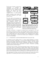
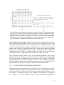
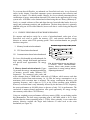
4.1 A CLUSTER-WIDE POWER MEASUREMENT SYSTEM
Figure 1 shows the prototype system we created for power-performance profiling. We
measure the power consumption of the major computing resources (i.e. CPU, memory,
disk, and NIC) on the slave nodes in a 32-node Beowulf. Each slave node has one
933MHz Intel Pentium III processor, 4 256M SDRAM modules, one 15.3GB IBM
DTLA-307015 DeskStar hard drive, and one Intel 82559 Ethernet Pro 100 onboard
Ethernet controller.
ATX extension cables connect the tested node to a group of 0.1 ohm sensor resistors on a
circuit board. The voltage on each resistor is measured with one RadioShack 46-range
digital multi meter 22-812 that has been attached to a multi port RS232 serial adapter
plugged into a data collection computer running Linux. We measure 10 power points
using 10 independent multi meters between the power supply and components
simultaneously.
Fig. 1. Our system prototype enables measurement of cluster power at component
granularity. For scalability, we assume the nodes are homogeneous. Thus, one node is
profiled and software is used to remap applications when workloads are non-uniform. A
separate PC collects data directly from the multimeters and uses time stamps to synchronize
measured data to an application.
The meters broadcast live measurements to the data collection computer for data logging
and processing through their RS232 connections. Each meter sends 4 samples per second
to the data collection computer.
11
Currently, this system measures one slave node at a time. The power consumed by a
parallel application requires summation of the power consumption on all nodes used by
the application. Therefore, we first measure a second node to confirm that power
measurements are nearly identical across like systems, and then use node remapping to
study the effective power properties of different nodes in the cluster without requiring
additional equipment. To ensure confidence in our results, we complete each experiment
at least 5 times based on our observations of variability.
Node remapping works as follows. Suppose we are running a parallel workload on M
nodes, we fix the measurement equipment to one physical node (e.g. node #1) and
repeatedly run the same workload M times. Each time we map the tested physical node to
a different virtual node. Since all slave nodes are identical (as they should be and we
experimentally confirmed), we use the M independent measurements on one node to
emulate one measurement on M nodes.
4.1.1 ISOLATING POWER BY COMPONENT
For parallel applications, a cluster can be abstracted as a group of identical nodes
consisting of CPU, memory, disk, and network interface. The power consumed by a
parallel application is computed by equations presented in section 2 with direct or derived
power measurement for each component.
In our prototype system, the mother board and disk on each slave node are connected to a
250 Watt ATX power supply through one ATX main power connector and one ATX
peripheral power connector respectively. We experimentally deduce the correspondence
between ATX power connectors and node components.
Since disk is connected to a peripheral power connection independently, its power
consumption can be directly measured through +12VDC and +5VDC pins on the
peripheral power connect. To map the component on the motherboard with the pins on
the main power connector, we observe the current changes on all non-COM pins by
adding/removing components and running different micro benchmarks which access
isolated components over time. Finally, we are able to conclude that the CPU is powered
through four +5VDC pins; memory, NIC and others are supplied through +3.3VDC pins;
the +12VDC feeds the CPU fan; and other pins are constant and small (or zero) current.
The CPU power consumption is obtained by measuring all +5VDC pins directly.
12
The idle part of memory system power
consumption
is
measured
by
extrapolation. Each slave node in the
prototype has four 256MB memory
modules. We measure the power
consumptions of the slave node
configured with 1, 2, 3, and 4 memory
modules separately, then estimate the
idle power consumed by the whole
memory system.
The slave nodes in the prototype are
configured with onboard NIC. It is hard
to separate its power consumption from
other components directly. After,
observing that the total system power
consumption changes slightly when we
disable the NIC or pull out the network
cable and consulting the documentation
of the NIC (Intel 82559 Ethernet Pro
100), we approximate it with constant
value of 0.41 watt.
Meter Reader
Thread
pipe
Meter Reader
Thread
Meter Reader
Thread
pipe
pipe
Shared Memory
PowerMeter Control Thread
Power Data Log
Message Listener
PowerAnalyzer
Message Client
System Statues Log
Library Calls
Application
Library Calls
System Status Profiler
Fig. 2. Automation with software. We created
scalable, multi-threaded software to collect and
analyze power meter data in real time. An
application programmer interface was created
to control (i.e. start/stop/init) multimeters and to
enable synchronization with parallel codes.
For further verification, we compared our measured power consumption for CPU and
disk with the specifications provided by Intel and IBM separately and they matched well.
Also by running memory access micro benchmarks, we observed that if accessed data
size is located within L1/L2 cache, the memory power consumption doesn’t change;
while once main memory is accessed, the memory power consumption we measured
increases correspondingly.
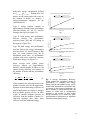
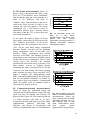
4.1.2 AUTOMATING CLUSTER POWER PROFILING AND ANALYSIS
To automate the entire profiling process we require enough multimeters to measure
directly, in real-time, a single node – 10 in our system. Under this constraint, we fully
automate data profiling, measurement and analysis by creating a tool suite named
PowerPack. PowerPack consists of utilities, benchmarks and libraries for controlling,
recording and processing power measurements in clusters. PowerPack’s profiling
software structure is shown in Figure 2
In PowerPack, the PowerMeter control thread reads data samples coming from a group of
meter readers which are controlled by globally shared variables. The control thread
modifies the shared variables according to messages received from applications running
on the cluster. Applications trigger message operations through a set of application level
library calls that synchronize the live profiling process with the application source code.
These application level library calls can be inserted into the source code of the profiled
applications. The commonly used subset of the power profile library API includes:
13
The power profile log and the system status log are processed with the PowerAnalyzer, a
software module that implements functions such as converting DC current to power,
interpolating between sampling points, decomposing pins power to component power,
computing power and energy consumed by applications and system, and performing
related statistical calculations.
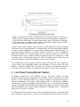
4.2 CLUSTER POWER PROFILES
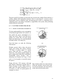
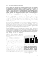
4.2.1 SINGLE NODE MEASUREMENTS
To better understand the power consumption
of distributed applications and systems, we
first profile the power consumption of a
single slave node. Figure 3 provides power
profiles for system idle (3a) and system
under load (3b) for the 171.swim benchmark
included in SPEC CPU2000 [44].
Power consumption distribution for system idle
System Power: 39 Watt
CPU
14%
Power Supply
33%
Memory
10%
Disk
11%
NIC
1%
Fans
23%
From this figure, we make the following
observations:
Whether system is idle or busy, the power
supply and cooling fans always consume
~20 Watts of power; about 1/2 system
power when idle and 1/3 system power
when busy. This means optimal design for
power supply and cooling fans could lead to
considerable power savings. This is
interesting but beyond the scope of this
work, so in our graphs we typically ignore
this power.
Other Chipset
8%
(a)
Power consumption distribution for
memory performance bound (171.swim)
System Power: 59 Watt
Power Supply
21%
CPU
35%
Fans
15%
Other Chipset
5%
NIC
1%
Memory
16%
Disk
7%
(b)
During idle time, CPU, memory, disk and
other chipset components consume about 17
Watts of power in total. When system is
under load, CPU power dominates (e.g. for
171.swim, it is 35% of system power; for
164.gzip, it is 48%).
Fig. 3. Power profiles for a single node (a)
during idle operation, and (b) under load.
As the load increases, CPU and memory
power dominate total system power.
14
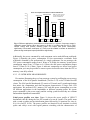
Power Consumption Distribution for Different Workloads
40.0
CPU-bound
35.0
memory-bound
Note: only power consumed
by CPU, memory, disk and
NIC are considered here
30.0
network-bound
25.0
disk-bound
20.0
15.0
10.0
5.0
0.0
idle
171.swim
164.gzip
CPU
Memory
cp
Disk
scp
NIC
Fig. 4. Different applications stress different components in a system. Component usage is
reflected in power profiles. When the system is not idle, it is unlikely that the CPU is 100%
utilized. During such periods, reducing power can impact total power consumption
significantly. Power-aware techniques (e.g. DVS) must be studied in clusters to determine if
power savings techniques impact performance significantly.
Additionally, the power consumed by each component varies under different workloads.
Figure 4 illustrates the power consumption of four representative workloads. Each
workload is bounded by the performance of a single component. For our prototype, the
CPU power consumption ranges from 6 Watts to 28 Watts; the memory system power
consumption ranges from 3.6 Watts to 9.4 Watts; the disk power consumption ranges
from 4.2 Watts to 10.8 Watts. Figure 4 indicates component use affects total power
consumption yet it may be possible to conserve power in non-idle cases when the CPU or
memory is not fully utilized.
4.2.2 CLUSTER-WIDE MEASUREMENTS
We continue illustrating the use of our prototype system by profiling the power-energy
consumption of the NAS parallel benchmarks (Version 2.4.1) on the 32-node Beowulf
cluster. The NAS parallel benchmarks [5] consist of 5 kernels and 3 pseudo-applications
that mimic the computation and data movement characteristics of large scale CFD
applications. We measured CPU, memory, NIC and disk power consumption over time
for different applications in the benchmarks at different operating points. We ignore
power consumed by the power supply and the cooling system because they are constant
and machine dependent as mentioned.
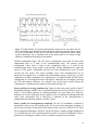
Nodal power profiles over time. Figure 5a shows the power profile of NPB FT
benchmark (class B) during the first 200 seconds of a run on 4 nodes. The profile starts
with a warm up phase and an initialization phase followed by N iterations (for class A,
N=6; for class B, N=20). The power profiles are identical for all iterations in which
spikes and valleys occur with regular patterns coinciding with the characteristics of
15
(a)
(b)
Fig. 5. FT Power Profiles. (a) The first 200 seconds of power use on one node of four for
the FT benchmark, class B workload. Note component results are overlaid along the y-axis
for ease of presentation. Power use for CPU and memory dominate and closely reflect
system performance. (b) An expanded view of the power profile of FT during a single
iteration of computation followed by communication.
different computation stages. The CPU power consumption varies from 25 watts in the
computation stage to 6 watts in the communication stage. The memory power
consumption varies from 9 watts in the computation stage to 4 watts in the
communication stage. Power trends in the memory during computation are often the
inverse of CPU power. Additionally, the disk uses near constant power since FT rarely
accesses the file system. NIC power probably varies with communication, but as
discussed, we emulate it as a constant since the maximum usage is quite low (.4 watts)
compared to all other components. For simplification, we ignore the disk and NIC power
consumption in succeeding discussions and figures where they do not change, focusing
on CPU and memory behavior. An in-depth view of the power profile during one
(computation + communication) iteration is presented in Figure 5b.
Power profiles for varying problem sizes. Figure 6a shows the power profile of the FT
benchmark (using the smaller class A workload) during the first 50 seconds of a run on 4
nodes. FT has similar patterns for different problem sizes (see Figure 5a). However,
iterations are shorter in duration for the smaller (class A) problem set making peaks and
values more pronounced; this is effectively a reduction in the communication to
computation ratio when the number of nodes is fixed.
Power profiles for heterogeneous workloads. For the FT benchmark, workload is
distributed evenly across all working nodes. We use our node remapping technique to
provide power profiles for all nodes in the cluster (in this case just 4 nodes). For FT, there
are no significant differences. However, Figure 6b shows a counter example snapshot for
a 10 second interval of SP synchronized across nodes. For the SP benchmark, Class A
problem sizes running on 4 nodes result in varied power profiles for each node.
16
(a)
(b)
Fig. 6. (a) The first 50 seconds of power use on one node of four for the FT benchmark, class
A workload. For smaller workloads running this application, trends are the same while data
points are slightly more pronounced since communication to computation ratios have changed
significantly with the change in workload. (b) Power use for code SP that exhibits
heterogeneous performance and power behavior across nodes. Note: x-axis is overlaid for
ease of presentation – repeats 20-30 second time interval for each node.
Power profiles for varying node counts. The power profile of parallel applications also
varies with the number of nodes used in the execution if we fix problem size (i.e. strong
scaling). We have profiled the power consumption for all the NPB benchmarks on all
execution nodes with different numbers of processors (up to 32) and several classes of
problem sizes. Figure 9a-c provides an overview of the profile variations on different
system scales for benchmarks FT, EP, and MG. These figures show segments of
synchronized power profiles for different number of nodes; all the power profiles
correspond to the same computing phase in the application on the same node.
These snapshots illustrate profile results for distributed benchmarks using various
numbers of nodes under Class A workload. Due to space limitations in a single graph,
here we focus on power amplitude only, so each time interval is simply a fixed length
snapshot (though the x-axis does not appear to scale). For FT and MG, the profiles are
similar for different system scale except the average power decreases with the number of
execution nodes; for EP, the power profile is identical for all execution nodes.
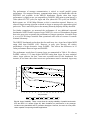
4.2.3 CLUSTER ENERGY-PERFORMANCE EFFICIENCY
For parallel systems and applications, we would like to use E (see Equation 6) to reflect
energy efficiency, and use D to reflect performance efficiency. To compare the energyperformance behavior of different parallel applications such as NPB benchmarks, we use
two metrics: 1) normalized delay or the speedup (from Equation 3) defined as
D# of node =1 D# of node =n ; and 2) normalized system energy, or the ratio of single-node to
17
Performance and Energy Consumption for EP (class A) code
Performance Speedup
14
12
10
8
6
4
Type I: energy remains constant or
approximately constant while performance
increases linearly. EP, SP, LU and BT
belong to this type (see Figure 7a).
Type III: both energy and performance
increase linearly but energy consumption
increases faster. FT and IS belong to this
type. For small problem sizes, the IS
benchmark gains little in performance
speedup using more nodes but consumes
much more energy (see Figure 7c).
2
0
1
2
3
4
5
6
7
8
9
10
11
12
13
14
15
16
15
16
15
16
Number of Nodes
(a)
Performance and Energy Consumption for MG (class A) code
Performance Speedup
Normalized System Energy
8
7
6
Normalized Value
Type II: both energy and performance
increase
linearly
but
performance
increases faster. MG and CG belong to
this type (see Figure 7b).
Normalized System Energy
16
Normalized Value
multi-node energy consumption, defined
as E # of node =n E # of node =1 . Plotting these two
metrics on the same graph with x-axis as
the number of nodes, we identify 3
energy-performance categories for the
codes measured.
5
4
3
2
1
0
1
2
3
4
5
6
7
8
9
10
11
12
13
14
Number of Nodes
(b)
Performance and Energy Consumption for FT (class A) code
Performance Speedup
Normalized System Energy
8
7
6
Normailzed Value
Since average total system power
increases linearly (or approximately
linearly) with the number of nodes, we can
express energy efficiency as a function of
the number of nodes and the performance
efficiency:
5
4
3
2
1
0
1
2
3
4
5
6
7
8
9
10
11
12
13
14
Numbe r of Node s
(c)
E n Pn ⋅ Dn Pn Dn n ⋅ Dn
=
=
⋅
≈
E1
P1 ⋅ D1
P1 D1
D1
(7).
In this equation, the subscript refers to the
number of nodes used by the application.
Equation 8 shows that energy efficiency of
parallel applications on clusters is strongly
tied to parallel speedup (D1/Dn). In other
words, as parallel programs increase in
efficiency with the number of nodes (i.e.
improved speedup) they make more
efficient use of the additional energy.
Fig. 7. Energy Performance Efficiency.
These graphs use normalized values for
performance (i.e. speedup) and energy.
Energy reflects total system energy. (a) EP
shows linear performance improvement with
no change in total energy consumption. (b)
MG is capable of some speedup with the
number of nodes with a corresponding
increase in the amount of total system
energy necessary. (c) FT shows only minor
improvements in performance for significant
increases in total system energy.
18
4.2.4 APPLICATION CHARACTERISTICS
The power profiles observed are regular and coincide with the computation and
communication characteristics of the codes measured. Patterns may vary by node,
application, component and workload, but the interaction or interdependency among
CPU, memory, disk and NIC have definite patterns. This is particularly obvious in the FT
code illustrated in the t1 through t13 labels in Figure 5b. FT phases include computation
(t1), reduce communication (t2), computation (t3:t4) and all-to-all communication
(t5:t11). More generally, we also observe the following for all codes:
1. CPU power consumption decreases when memory power increases. This reflects the
classic memory wall problem where access to memory is slow, inevitably causing
stalls (low power operations) on the CPU.
2. Both CPU power and memory power decrease with message communication. This is
analogous to the memory wall problem where the CPU stalls while waiting on
communication. This can be alleviated by non-blocking messages, but this was not
observed in the Ethernet-based system under study.
3. For all the codes studied (except EP), the normalized energy consumption decreases
as the number of nodes increases. In other words, while performance is gained from
application speedup, there is a considerable price paid in increased total system
energy.
4. Communication distance and message size affect the power profile patterns. For
example, LU has short and shallow power profiles while FT phases are significantly
longer. This highlights possible opportunities for power and energy savings
(discussed next).
4.2.5 RESOURCE SCHEDULING
We mentioned an application’s energy efficiency is dependent on its speedup or parallel
efficiency. For certain applications such as FT and MG, we can achieve speedup by
running on more processors while increasing total energy consumption. The subjective
question remains as to whether the performance gain was worth the additional resources.
Our measurements indicate there are tradeoffs between power, energy, and performance
that should be considered to determine the best resource “operating points” or the best
configuration in number of nodes (NP) based on the user’s needs.
For performance-constrained systems, the best operating points will be those that
minimize delay (D). For power-constrained systems, the best operating points will be
those that minimize power (P) or energy (E). For systems where power-performance
must be balanced, the choice of appropriate metric is subjective. The energy-delay
product (see POWER-PERFORMANCE TRADEOFFS, page 5) is commonly used as a
single metric to weigh the effects of power and performance.
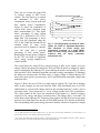
Figure 8 presents the relationships between four metrics (normalized D and E, EDP, and
ED2P) and the number of nodes for the MG benchmark (class A). To minimize energy
19
Fig. 8. To determine the number of nodal resources that provides the best rate of return on
energy usage is a subjective process. Different metrics recommend different configurations.
For the MG code shown here, minimizing delay means using 32 processors; minimizing
energy means using 1 processor; the EDP metric recommends 8 processors while the ED2P
metric recommends 16 processors. Note: y-axis in log.
(E), the system should schedule only one node to run the application which corresponds
in this case to the worst performance. To minimize delay (D), the system should schedule
32 nodes to run the application or 6 times speedup for more than 4 times the energy. For
power-performance efficiency, a scheduler using the EDP metric would recommend 8
nodes for a speedup of 2.7 and an energy cost of 1.7 times the energy of 1 node. Using
the ED2P metric a smart scheduler would recommend 16 nodes for a speedup of 4.1 and
an energy cost of 2.4 times the energy of 1 node. For fairness, the average delay and
energy consumption obtained from multiple runs are used in Figure 8.
For existing cluster systems, power-conscious resource allocation can lead to significant
energy savings with controllable impact on performance. Of course, there are more
details to consider including how to provide the scheduler with application-specific
information. This is the subject of ongoing research in power-aware cluster computing.
5 Low Power Computational Clusters
To address operating cost and reliability concerns, large-scale systems are being
developed with low power components. This strategy, used in construction of Green
Destiny [70] and IBM BlueGene/L [8], requires changes in architectural design to
improve performance. For example, Green Destiny relies on driving the Transmeta
Crusoe processor [52] development while BlueGene/L uses a version of the embedded
PowerPC chip modified with additional floating point support. In essence, the resulting
high-end machines are no longer strictly composed of commodity parts – making this
approach very expensive to sustain.
To illustrate the pros and cons of a low power computational cluster, we developed the
Argus prototype, a high density, low power supercomputer built from an IXIA network
20
analyzer chassis and load modules. The prototype is configured as a diskless cluster
scalable to 128 processors in a single 9U chassis. The entire system has a footprint of 1/4
meter2 (2.5 ft2), a volume of 0.09 meter3 (3.3 ft3) and maximum power consumption of
less than 2200 watts. In this section, we compare and contrast the characteristics of Argus
against various machines including our 32-node Beowulf and Green Destiny.
5.1 ARGUS: LOW POWER CLUSTER COMPUTER
Computing resources may be special purpose (e.g. Earth Simulator) or general purpose
(e.g. network of workstations). While these high-end systems often provide unmatched
computing power, they are extremely expensive, requiring special cooling systems,
enormous amounts of power and dedicated building space to ensure reliability. It is
common for a supercomputing resource to encompass an entire building and consume
tens of megawatts of power.
In contrast low-power, high-throughput, high-density systems are typically designed for a
single task (e.g. image processing). These machines offer exceptional speed (and often
guaranteed performance) for certain applications. However, design constraints including
performance, power, and space make them expensive to develop and difficult to migrate
to future generation systems.
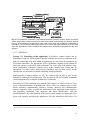
The chassis contains a power supply and
distribution unit, cooling system, and runs
windows and proprietary software (IX server and
IX router). Multiple (up to 16) Load Modules plug
into the chassis and communicate with the chassis
and each other via an IX Bus (mainly used for
system management, much too slow for message
P
C
M
P
C
M
P
C
P
C
F
P
M G
A
M
IXIA Chassis Load Module #N
NFS Server
To External Network
Figure 9 is a detailed diagram of the prototype
architecture we call Argus. This architecture
consists of four sets of separate components: the
IXIA chassis, the IXIA Load Modules, the multi
port fast Ethernet switch and an NFS server.
IX Server
5.1.1 SYSTEM DESIGN
Load Module #1
Multiport switch
IX Bus
IX Router
We propose an alternative approach augmenting a specialized system (i.e. an Ixia
network analyzer) that is designed for a commodity marketplace under performance,
power, and space constraints. Though the original Ixia machine is designed for a single
task, we have created a configuration that
provides general-purpose high-end parallel
processing in a Linux environment. Our system
P
C M
provides computational power surpassing Green
F
P
C M P
Destiny
[30,
70]
(another
low-power
P
C M G
supercomputer) while decreasing volume by a
A
P
C M
factor of 3.
Fig. 9. The Hardware Architecture
Argus. Up to 16 Load Modules are
supported in a single IXIA 1600T
chassis. A single bus interconnects
modules and the chassis PC while
external disks and the cluster frontend are connected via an Ethernet
switch.
P=processor,
C=Cache,
M=Memory.
21
transfer). Each Load Module provides up to 8 RISC processors (called port processors) in
a dense form factor and each processor has its own operating system, cache (L1 and L2),
main memory and network interface. Additional FPGA elements on each Load Module
aid real-time analysis of network traffic. Though the performance abilities of these
FPGAs have merit, we omit them from consideration for two reasons: 1) reprogramming
is difficult and time consuming, and 2) it is likely FPGA elements will not appear in
succeeding generation Load Modules to reduce unit cost.
There is no disk on each Load Module. We allocate a small portion of memory at each
port to store an embedded version of the Linux OS kernel and application downloaded
from the IX Server. An external Linux machine running NFS file server is used to
provide external storage for each node. A possible improvement is to use networked
memory as secondary storage but we did not attempt this in the initial prototype. Due to
cost considerations, although the Load Modules support 1000 Mbps Ethernet on copper,
we used a readily available switch operating at 100 Mbps.
The first version of the Argus prototype is implemented with one IXIA 1600T chassis
and 4 LM1000TXS4 Load Modules (See http://www.ixiacom.com/library/catalog/ for
specification) [20] configured as a 16-node distributed memory system, i.e., each port
processor is considered as an individual node.
Another option is to configure each Load Module as an SMP node. This option requires
use of the IxBus between Load Modules. The IxBus bus (and the PowerPC 750CXe
processor) does not maintain cache coherence and has limited bandwidth. Thus, early on
we eliminated this option from consideration since software-driven cache coherence will
limit performance drastically. We opted to communicate data between all processors
through the Ethernet connection. Hence one recommendation for future implementations
is to significantly increase the performance and capabilities of the IX Bus. This could
result in a cluster of SMPs architecture allowing hybrid communications for improved
performance.
Each LM1000TXS4 Load Module provides four 1392 MIPS PowerPC 750CXe RISC
processors [45] and each processor has one 128MB memory module and one network
port with auto-negotiating 10/100/1000 Mbps Copper Ethernet interface. The 1392 MIPS
PowerPC 750CXe CPU employs 0.18 micrometer CMOS copper technology, running at
600 MHz with 6.0W typical power dissipation. This CPU has independent on-chip 32K
bytes, eight-way set associative, physically addressed caches for instructions and data.
The 256KB L2 cache is implemented with on-chip, two-way set associative memories
and synchronous SRAM for data storage. The external SRAM are accessed through a
dedicated L2 cache port. The PowerPC 750CXe processor can complete two instructions
per CPU cycle. It incorporates 6 execution units including one floating-point unit, one
branch processing unit, one system register unit, one load/store unit and two integer units.
Therefore, the theoretical peak performance of the PowerPC 750CXe is 1200 MIPS for
integer operations and 600 MFLOPS for floating-point operations.
In Argus, message passing (i.e. MPI) is chosen as the model of parallel computation. We
ported gcc3.2.2 and glib for PowerPC 750 CXe to provide a useful development
22
environment. MPICH 1.2.5 (the MPI implementation from Argonne National Lab and
Michigan State University) and a series of benchmarks have been built and installed on
Argus. Following our augmentation, Argus resembles a standard Linux-based cluster
running existing software packages and compiling new applications.
5.1.2 LOW POWER CLUSTER METRICS
According to design priorities, general-purpose clusters can be classified into four
categories:
Performance: These are traditional high-performance systems (e.g. Earth Simulator)
where performance (GFLOPS) is the absolute priority.
Cost: These are systems built to maximize the performance/cost ratio (GFLOPS/$) using
commercial-off-the-shelf components (e.g. Beowulf).
Power: These systems are designed for reduced power (GFLOPS/Watt) to improve
reliability (e.g. Green Destiny) using low-power components.
Density: These systems have specific space constraints requiring integration of
components in a dense form factor with specially designed size and shape (e.g. Green
Destiny) for a high performance/volume ratio (GFLOPS/ft3).
Though high performance systems are still a majority in the HPC community; low cost,
low power, low profile and high density systems are emerging. Blue Gene/L (IBM) [1]
and Green Destiny (LANL) are two examples designed under cost, power and space
constraints.
Argus is most comparable to Green Destiny. Green Destiny prioritizes reliability (i.e.
power consumption) though this results in a relatively small form factor. In contrast, the
Argus design prioritizes space providing general-purpose functionality not typical in
space-constrained systems. Both Green Destiny and Argus rely on system components
targeted at commodity markets.
Green Destiny uses the Transmeta Crusoe TM5600 CPU for low power and high density.
Each blade of Green Destiny combines server hardware, such as CPU, memory, and the
network controller into a single expansion card. Argus uses the PowerPC 750CXe
embedded microprocessor which consumes less power but matches the sustained
performance of the Transmeta Crusoe TM5600. Argus’ density comes at the expense of
mechanical parts (namely local disk) and multiple processors on each load module (or
blade). For perspective, 240 nodes in Green Destiny fill a single rack (about 25 ft3);
Argus can fit 128 nodes in 3.3 ft3. This diskless design makes Argus more dense and
mobile yet less suitable for applications requiring significant storage.
TCO Metrics. As Argus and Green Destiny are similar, we use the total cost of
ownership (TCO) metrics proposed by Feng et al [30] as the basis of evaluation. For
completeness, we also evaluate our system using traditional performance benchmarks.
23
TCO = AC + OC
(8).
AC = HWC + SWC
(9).
OC = SAC + PCC + SCC + DTC
(10).
TCO refers to all expenses related to acquisition, maintaining and operating the
computing system within an organization. Equations (8-10) provide TCO components
including acquisition cost (AC), operations cost (OC), hardware cost (HWC), software
cost (SWC), system-administration cost (SAC), power-consumption cost (PCC), spaceconsumption cost (SCC) and downtime cost (DTC). The ratio of total cost of ownership
(TCO) and the performance (GFLOPS) is designed to quantify the effective cost of a
distributed system.
According to a formula derived from Arrhenius’ Law2, component life expectancy
decreases 50% for every 10º C (18º F) temperature increase. Since system operating
temperature is roughly proportional to its power consumption, lower power consumption
implies longer component life expectancy and lower system failure rate. Since both
Argus and Green Destiny use low power processors, the performance to power ratio
(GFLOPS/watt) can be used to quantify power efficiency. A high GFLOPS/watt implies
lower power consumption for the same number of computations, and hence lower system
working temperature and higher system reliability (i.e. lower component failure rate).
Since both Argus and Green Destiny provide small form factors relative to traditional
high-end systems, the performance to space ratio (GFLOPS/ft2 for footprint and
GFLOPS/ft3 for volume) can be used to quantify computing density. Feng et al propose
the footprint as the metric of computing density [30]. While Argus performs well in this
regard for a very large system, we argue it is more precise to compare volume. We
provide both measurements in our results.
Benchmarks. We use an iterative benchmarking process to determine the system
performance characteristics of the Argus prototype for general comparison to a
performance/cost design (i.e. Beowulf) and to target future design improvements.
Benchmarking is performed at two levels:
Micro-benchmarks: Using several micro benchmarks such as LMBENCH [57],
MPPTEST [37], NSIEVE [49] and Livermore LOOPS [56], we provide detailed
performance measurements of the core components of the prototype CPU, memory
subsystem and communication subsystem.
Kernel application benchmarks: We use LINPACK [25] and the NAS Parallel
Benchmarks [5] to quantify performance of key application kernels in high performance
2
Reaction rate equation of Swedish physical chemist and Nobel Laureate Svante Arrhenius (1859-1927) is used to derive time to
failure as a function of e-Ea/KT, where Ea is activation energy (eV), K is Boltzman’s constant, and T is absolute temperature in Kelvin.
24
scientific computing. Performance bottlenecks in these applications may be explained by
measurements at the micro-benchmark level.
For direct performance comparisons, we use an on-site 32-node Beowulf cluster called
DANIEL. Each node on DANIEL is a 933MHZ Pentium III processor with 1 Gigabyte
memory running Red Hat Linux 8.0. The head node and all slave nodes are connected
with two 100M Ethernet switches. We expect DANIEL to out-perform Argus generally,
though our results normalized for clock rate (i.e. using machine clock cycles instead of
seconds) show performance is comparable given DANIEL is designed for
performance/cost and Argus for performance/space.
For direct measurements, we use standard UNIX system calls and timers when applicable
as well as hardware counters if available. Whenever possible, we use existing, widelyused tools (e.g. LMBENCH) to obtain measurements. All measurements are the average
or minimum results over multiple runs at various times of day to avoid outliers due to
local and machine-wide perturbations.
5.1.3 ANALYZING A LOW POWER CLUSTER DESIGN
Measured Cost, Power and Space Metrics. We make direct comparisons between
Argus, Green Destiny and DANIEL based on the aforementioned metrics. The results are
given in Table 1. Two Argus systems are considered: Argus64 and Argus128. Argus64 is
the 64-node update of our current prototype with the same Load Module. Argus128 is the
128-node update with the more advanced IXIA Application Load Module (ALM1000T8)
currently available [20]. Each ALM1000T8 load module has eight 1856 MIPS PowerPC
processors with Gigabit Ethernet interface and 1GB memory per processor. Space
efficiency is calculated by mounting 4 chassis' in a single 36U rack (excluding I/O node
and Ethernet switches to be comparable to Green Destiny). The LINPACK performance
of Argus64 is extrapolated from direct measurements on 16-nodes and the performance
of Argus128 is predicted using techniques similar to Feng et al. as 2×1.3 times the
performance of Argus64.
All data on the 32-node Beowulf, DANIEL is obtained from direct measurements. There
is no direct measurement of LINPACK performance for Green Destiny in the literature.
We use both the Tree Code performance as reported [70] and the estimated LINPACK
performance by Feng [29] for comparison denoted with parenthesis in Table 1.
We estimated the acquisition cost of Argus using prices published by IBM in June 2003
and industry practice. Each PowerPC 750Cxe costs less than $50. Considering memory
and other components, each ALM Load Module will cost less than $1000. Including
software and system design cost, each Load Module could sell for $5000-$10000.
Assuming the chassis costs another $10,000, the 128-node Argus may cost $90K-170K in
acquisition cost (AC). Following the same method proposed by Feng et al., the operating
cost (OC) of Argus is less than $10K. Therefore, we estimate the TCO of Argus128 is
below $200K. The downtime cost of DANIEL is not included when computing its TCO
since it is a research system and often purposely rebooted before and after experiments.
25
Table 1. Cost, Power, and Space Efficiency. For Green Destiny, the first value corresponds to
its Tree Code performance; the second value in parenthesis is its estimated LINPACK
performance. All other systems use LINPACK performance. The downtime cost of DANIEL is
not included when computing its TCO since it is a research system and often purposely
rebooted before and after experiments. The TCO of the 240-node Green Destiny is estimated
based on the data of its 24-node system.
Machine
DANIEL
Green Destiny
ARGUS64
ARGUS128
CPUs
32
240
64
128
Performance
(GFLOPS)
17
39 (101)
13
34
Area (foot2)
12
6
2.5
2.5
TCO ( $K)
100
350
100-150
100-200
Volume(foot3)
50
30
3.3
3.3
Power(kW)
2
5.2
1
2
GFLOPS/proc
0.53
0.16
(0.42)
0.20
0.27
GFLOPS
Per Chassis
0.53
3.9
13
34
TCO Efficiency
(GFLOPS/K$)
0.17
0.11
(0.29)
0.08~0.13
0.17~0.34
Computing Density
(GFLOPS/foot3)
0.34
1.3 (3.3)
3.9
10.3
Space
Efficiency
(GFLOPS/foot2)
1.4
6.5 (16.8)
20.8
54.4
Power Efficiency
(GFLOPS/foot3)
8.5
7.5
(19.4)
13
17
The TCO of the 240-node Green Destiny is estimated based on the data of its 24-node
system.
Though TCO is suggested as a better metric than acquisition cost, the estimation of
downtime cost (DTC) is subjective while the acquisition cost is the largest component of
TCO. Though, these three systems have similar TCO performance, Green Destiny and
Argus have larger acquisition cost than DANIEL due to their initial system design cost.
System design cost is high in both cases since the design cost has not been amortized
over the market size – which would effectively occur as production matures.
The Argus128 is built with a single IXIA 1600T chassis with 16 blades where each blade
contains 8 CPUs. The chassis occupies 44.5×39.9×52 cm3 (about 0.09 m3 or 3.3 ft3).
Green Destiny consists of 10 chassis; each chassis contains 10 blades; and each blade has
only one CPU. DANIEL includes 32 rack-dense server nodes and each node has one
CPU.
26
Due to the large difference in system
footprints (50 ft3 for DANIEL, 30 ft3 for
Green Destiny and 3.3 ft3 for Argus) and
relatively small difference in single
processor performance (711 MFLOPS for
DANIEL, 600 MFLOPS for Green
Destiny and 300 MFLOPS for Argus),
Argus has the highest computing density,
30 times higher than DANIEL, and 3
times higher than Green Destiny.
Table 1 shows Argus128 is twice as
efficient as DANIEL and about the same
as Green Destiny. This observation
contradicts our expectations that Argus
should fair better against Green Destiny in
power efficiency. However upon further
investigation we suspect either 1) the
Argus cooling system is less efficient (or
works harder given the processor density),
2) our use of peak power consumption on
Argus compared to average consumption
on Green Destiny is unfair, 3) the Green
Destiny LINPACK projections (not
measured directly) provided in the
literature are overly optimistic, or 4) some
combination thereof. In any case, our
results indicate power efficiency should be
revisited in succeeding designs though the
results are respectable particularly given
the processor density.
Table 2. Memory System Performance
ARGUS
DANIEL
CPU Clock Rate
Parameters
600MHz
922MHz
Clock Cycle Time
1.667ns
1.085ns
32KB
16KB
3.37ns?2 cycles
3.26ns?3 cycles
256KB
256KB
19.3ns?12cycles
7.6ns ? 7 cycles
128MB
1GB
220ns?132 cycles
153ns?141 cycles
Memory Read Bandwidth
146~2340MB/s
514~3580MB/s
Memory Write Bandwidth
98~2375MB/s
162~3366MB/s
L1 Data Cache Size
L1 Data Cache Latency
L2 Data Cache Size
L2 Data Cache Latency
Memory Size
Memory Latency
Table 3. Instruction Performance. IPC:
Instructions per clock, MIPS: Millions of
instructions per second, I: Integer, F: Single
precision floating point; D: Double precision
floating point.
Instruction
I-BIT
I-ADD
I-MUL
I-DIV
I-MOD
F-ADD
F-MUL
F-DIV
D-ADD
D-MUL
D-DIV
Cycles
1
1
2
20
24
3
3
18
3
4
32
ARGUS
IPC
1.5
2.0
1.0
1.0
1.0
3.0
3.0
1.0
3.0
2.0
1.0
MIPS
900
1200
300
30
25
600
600
33
600
300
19
Cycles
1
1
4
39
42
3
5
23.6
3
5
23.6
DANIEL
IPC
1.93
1.56
3.81
1.08
1.08
2.50
2.50
1.08
2.50
2.50
1.08
MIPS
1771
1393
880
36
24
764
460
42
764
460
42
Performance results. A single RLX
System 324 chassis with 24 blades from Green Destiny delivers 3.6 GFLOPS computing
capability for the Tree Code benchmark. A single IXIA 1600T with 16 Load Modules
achieves 34 GFLOPS for the LINPACK benchmark. Due to the varying number of
processors in each system, the performance per chassis and performance per processor
are used in our performance comparisons. Table 1 shows DANIEL achieves the best
performance per processor and Argus achieves the worst. Argus has poor performance on
double MUL operation (discussed in the next section) which dominates operations in
LINPACK. Argus performs better for integer and single precision float operations. Green
Destiny outperforms Argus on multiply operations since designers were able to work
with Transmeta engineers to optimize the floating point translation of the Transmeta
processor.
Memory hierarchy performance (latency and bandwidth) is measured using the
lat_mem_rd and bw_mem_xx tools in the LMBENCH suite. The results are summarized
27
in Table 2. DANIEL, using its high-power,
high-profile off-the-shelf Intel technology,
outperforms Argus at each level in the
memory hierarchy in raw performance
(time). Normalizing with respect to cycles
however, shows how clock rate partially
explains the disparity. The resulting
"relative performance" between DANIEL
and Argus is more promising. Argus
performs 50% better than Daniel at the L1
level, 6% better at the main memory level,
but much worse at the L2 level. Increasing
the clock rate of the PowerPC processor
and the L2 implementation in Argus
would
improve
raw
performance
considerably.
Table 4. Livermore Loops. NORM:
normalized performance, obtained by
dividing MFLOPS by CPU clock rate
ARGUS
DANIEL
MFLOPS NORM. MFLOPS NORM.
Maximum Rate
731.5
1.22
1281.9
1.37
Quartile Q3
225.0
0.38
377.6
0.40
Average Rate
174.5
0.29
278.9
0.30
Geometric Mean
135.5
0.23
207.2
0.22
Median Q2
141.6
0.24
222.2
0.24
Harmonic Mean
106.6
0.18
133.6
0.14
Quartile Q1
66.4
0.11
132.6
0.14
Minimum Rate
46.2
0.08
20.0
0.02
Standard Dev
133.8
0.22
208.5
0.22
Average Efficiency
18.52%
16.16%
IPC is the number of instructions executed
Mean Precision (digits)
6.24
6.35
per clock cycle. Throughput is the number
of instructions executed per second (or
IPC x clock_cycle). Peak throughput is the
Table 5. Linpack Results on Argus
maximum throughput possible on a given
NP
Problem Size
GFLOPS
GFLOPS/proc
Speedup
architecture. Peak throughput is only
1
3000
0.297
0.297
1.00
2
3000
0.496
0.248
1.67
attained when ideal IPC (optimal
4
5000
0.876
0.219
2.95
8
8000
1.757
0.221
5.91
instruction-level parallelism) is sustained
16
12000
3.393
0.212
11.42
on the processor. Memory accesses, data
dependencies, branching, and other code
characteristics
limit
the
achieved
throughput on the processor. Using microbenchmarks, Table 6. Parallel Benchmark
we measured the peak throughput for various Results on Argus
instruction types on the machines under study.
Performance (MOP/second)
CODE
NP=1
NP=4
NP=16
Table 3 shows the results of our throughput
CG
19.61
46.04
88.12
experiments.
Integer
performance
typically
EP
1.69
6.75
24.08
outperforms floating point performance on Argus. For
IS
4.06
3.62
18.02
DANIEL (the Intel architecture) floating point (F-xxx
in Table 3) and double (D-xxx in Table 3)
LU
48.66
188.24
674.62
performances are comparable for ADD, MUL, and
MG
45.50
84.51
233.36
DIV respectively. This is not true for Argus where FBT
40.04
131.76
436.29
MUL and D-MUL are significantly different as
SP
28.72
90.99
299.71
observed in our LINPACK measurements. We expect
the modified version of the PowerPC architecture
(with an additional floating point unit) present in IBM
Bluegene\L will equalize the performance difference with the Intel architecture in future
systems. CPU throughput measurements normalized for clock rates (MIPS) show Argus
performs better than DANIEL for integer ADD/DIV/MOD, float ADD/MUL and double
ADD instructions, but worse for integer MUL and double DIV instructions.
28
The performance of message communication is critical to overall parallel system
performance. We measured memory communication latency and bandwidth with the
MPPTEST tool available in the MPICH distribution. Results show that Argus
performance is slightly worse yet comparable to DANIEL. MPI point-to-point latency is
104ns (about 62 CPU cycles) on Argus and 87ns (about 80 CPU cycles) on DANIEL.
Both systems use 10/100 Mbps Ethernet so this is somewhat expected. However, we
observed larger message injection overhead on Argus as message size approaches typical
packet size. This is most likely due to the memory hierarchy disparity already described.
For further comparison, we measured the performance of two additional sequential
benchmarks: NSIEVE and Livermore Loops. NSIEVE is a sieve of Eratosthenes program
that varies array sizes to quantify the performance of integer operations. Livermore loops
is a set of 24 DO-loops extracted from operational code used at Lawrence Livermore
National Laboratory.
The NSIEVE benchmark results show that for small array size, Argus has a higher MIPS
rating (980) than DANIEL (945). However, as array sizes increase, the relative
performance of Argus decreases versus DANIEL. This reflects the differences in L2
cache performance between Argus and DANIEL.
Normalized MOP/second/processor
The performance results from Livermore loops are summarized in Table 4. We observe
DANIEL achieves 1.5-2 times higher MFLOPS rating than Argus for most statistical
values, Argus achieves the best, worst-case execution time for this benchmark. For
instance, in real time codes where worst-case performance must be assumed, Argus may
1
0.8
0.6
0.4
0.2
0
1
2
3
4
5
6
7
8
9
10
11
12
13
14
15
16
# of processors
CG
EP
IS
LU
MG
SP
BT
Fig. 10. Argus Scalability. These curves show the varying scalability of parallel benchmarks
from the NPB 2.4.1 release (Class W). Main limitations on performance in the prototype
include memory bandwidth and FP operation throughput. However, the result is a low power
cluster capable of computing scientific applications.
29
be a better choice. However, examining performance normalized for clock rates (NORM)
on this benchmark, the two systems perform similarly.
The Argus prototype architecture can execute both commercial and scientific
applications. In this paper, we focus on scientific applications and provide results for two
benchmark suites: LINPACK [25] and the NAS parallel benchmarks [5]. Since we
already established the performance difference between Argus and DANIEL for single
node (see previous section), here we only discuss the parallel performance of Argus.
LINPACK is arguably the most widely used benchmark for scientific applications and its
measurements form the basis for the Top500 list [63] of fastest supercomputers in the
world. Our measurements use HPL, a parallel version of the linear algebra subroutines in
LINPACK that solve a (random) dense linear system in double precision (64-bit)
arithmetic on distributed-memory computers. HPL provides the ability to scale workloads
for better performance by adjusting array sizes. To ensure good performance, we
compiled and installed the BLAS libraries with the aid of ATLAS (Automatically Tuned
Linear Algebra Software). Table 5 shows the LINPACK benchmark results on the 16node Argus prototype. The prototype achieves 3.4 GFLOPS, about 210 MFLOPS each
node or 70% peak throughput of “double MUL” operations.
The NAS Parallel Benchmark (NPB) is a set of 8 programs designed to help evaluate the
performance of parallel supercomputers. This benchmark suite consists of five
application kernels and three pseudo-applications derived from computational fluid
dynamics applications. These benchmarks are characterized with different
computation/communication ratios described in [5]. The raw performance of NPB 2.4.1
with a problem size of W on Argus is shown in Table 6. To better identify the
performance trends, Figure 10 provides the scalability of Argus under strong scaling (i.e.
fixed problem size and increasing number of processors).
For 16 nodes, EP and LU show the best scalability. The embarrassingly-parallel code
(EP) should achieve linear speedup since little communication is present. LU achieves
super-linear speedup that appears to be levelling off. As working set size remains fixed
with increases in the number of processors, communication is minimal (i.e. strong or
fixed-size scaling). Super-linear performance is achieved as the working set gets smaller
and smaller on a per node basis.
The curve of IS initially drops but then grows with the number of nodes. These codes
stress communication performance. The levelling off of performance indicates the
communication costs are not saturating the Ethernet interconnect up to 16 nodes.
The other four curves (SP, BT, CG and MG) have similar trends but different slopes. The
performance of these codes reflects the communication to computation ratio. EP and LU
are dominated by computation. IS and FT are dominated by communication. These codes
sit somewhere in between. Trends here are similar (though less pronounced) than the
communication-bound codes. These codes (SP, BT, CG, and MG) are more sensitive to
the number of nodes as it affects the number of communications. Performance then is
likely to move downward with the number of nodes until a plateau is reached prior to
30
network saturation (i.e. similar to the plateau in IS and FT performance). At some later
point all of these codes will reach the limits of either the input data set size (Amdahl’s
Law) or the interconnect technology (saturation) where performance will drop drastically
again. Our system is too small to observe these types of problems, so this is the subject of
future work.
5.1.4 LESSONS FROM A LOW POWER CLUSTER DESIGN
Argus exemplifies an architectural design with trade-offs between performance, cost,
space and power. The Argus prototype is a new approach to cluster computing that uses
the aggregate processing elements on network analysis Load Modules for parallel
computing. The analysis shows this architecture has advantages such as high scalability,
small volumetric footprint, reduced power, high availability, and ultra-high processor
density.
Argus achieves higher computing efficiency than Green Destiny, a comparable system
with similar power efficiency. Argus is capable of packing more processors per blade
than Green Destiny at present though future versions of both machines will undoubtedly
address this.
The benchmarking measurements and comparisons with DANIEL indicate that the
current Argus prototype has two major performance limitations due to the architectural
characteristics of the embedded PowerPC processor: L2 cache latency and hardware
support for double precision. Also the communication overhead on the processing node
should and could be improved through system-specific hardware and software tuning of
MPI. Furthermore, results from a larger prototype with a faster interconnect would allow
more comprehensive scalability analyses.
There are two concerns with the low power cluster design approach highlighted by our
experiments with Argus. First, performance is not considered a critical design constraint.
In all low power approaches including Argus, Green Destiny and IBM BlueGene \L,
performance is sacrificed to reduce the power consumption of the machine. BlueGene \L
has been the most successful at overcoming this constraint by 1) redesign of the PowerPC
embedded architecture to support double precision floating point operations, and 2)
custom design of a 130,000+ processor system.
Second, the low power approach is limited since it assumes all applications suffer from
poor power efficiency. This contradicts our earlier findings that the power needs of
applications vary significantly over time. Together, these observations motivate the need
for power-conscious approaches in high-performance that adapt to the performance
phases of applications.
6 Power-aware Computational Clusters
Recently, power has become a critical issue for large data centers. Studies of power
consumption and energy conservation on commercial servers have emerged. Bohrer et al
[9] found dynamic voltage and frequency scaling (DVFS) for processors is effective for
31
saving energy in web servers. Carrera et al [17] found multi-speed disks can save energy
up to 23% for network servers. Zhu et al [72, 73] combines several techniques including
multi-speed disks and data migration to reduce energy consumption while meeting
performance goals.
Power reduction becomes critical in high-performance computing to ensure reliability
and limit operating cost. Two kinds of systems are now built to accommodate these
goals: systems with low power components (discussed in the previous section [8, 31, 32])
and systems with power-aware components [43]. Energy reduction using power-aware
technologies had not been exploited in high-performance computing until our research
was launched in 2004 [15].
In contrast to Argus, Green Destiny and BlueGene/L, our power-aware approach for HPC
uses off-the-shelf DVS technologies3 in server-class systems to exploit scientific
workload characteristics. Power-aware clusters include components that have multiple
power/performance modes (e.g. CPU’s with DVS). The time spent within and
transitioning to/from these power/performance modes determines the delay (cost in
performance) and energy (cost in power, heat, etc.).
There are two ways to schedule DVS transitions. External distributed DVS scheduling
techniques are autonomous and control DVS power/performance modes in a cluster as
processes separate from the application under study. External schedulers may be systemdriven (e.g. the cpuspeed daemon) or user-driven (e.g. setting DVS from the command
line). Internal distributed DVS scheduling techniques use source-level performance
profiling to direct DVS power/performance modes with source-code instrumentation.
6.1 USING DVS IN HIGH-PERFORMANCE CLUSTERS
Dynamic Voltage Scaling (DVS) is a technology now common in high-performance
microprocessors [3, 46]. DVS works on a very simple principal: decreasing the supply
voltage to the CPU consumes less power.
As shown in Equation 4, the dynamic power consumption (P) of a CMOS-based
microprocessor is proportional to the product of total capacitance load (C), frequency (f),
the square of the supply voltage (V2), and percentage of active gates (A) or P≈ACV2f. As
shown in Equation 6, energy consumption (measured in joules) is reduced by lowering
the average power (Pavg) consumed for some duration or delay (D) or E=Pavg x D.
3
DVS capabilities are now available in server-class architectures including Intel Xeon (SE7520 chipset) and AMD Opteron (Tyan
s2882 board) dual processor nodes.
32
Normalized Delay and Energy for Swim
Normalized Energy
Normalized Delay
1.4
Normalized Values
There are two reasons for using DVS
to conserve energy in HPC server
clusters. The first reason is to exploit
the dominance of CPU power
consumption on the system node (and
thus cluster) power consumption.
Figure 3b shows the breakdown of
system node power obtained using
direct measurement [33]. This figure
shows percentage of total system
power for a Pentium III CPU (35%)
under load. This percentage is lower
(15%) but still significant when the
CPU is idle. While the Pentium III can
consume nearly 45 watts, recent
processors such as Itanium 2 consume
over 100 watts and a growing
percentage of total system power.
Reducing the average power consumed
by the CPU can result in significant
server energy savings magnified in
cluster systems.
1.2
1
0.8
0.6
0.4
0.2
0
600
800
1000
1200
1400
CPU Frequency (MHz)
Fig. 11: The energy-delay crescendo for swim
shows the effect of application-dependent
CPU slackness on (node) energy and
performance measured at a single NEMO
node. For swim, energy conservation can be
achieved
with
(at
times)
reasonable
performance loss.
The second reason for using DVS to conserve energy in HPC server clusters is to save
energy without increasing execution time. DVS provides the ability to adaptively reduce
power consumption. By reducing CPU power when peak speed is not needed (e.g. idle or
slack periods) a DVS scheduling algorithm can reduce energy consumption. To minimize
the impact on execution time we must ensure 1) supply voltage is reduced during CPU
times when peak speed is not necessary, and 2) period duration outweighs voltage state
transition costs4.
Figure 11 shows the use of DVS on a single node to exploit CPU slack due to memory
stalls. In this example we run swim from the SPEC 2000 benchmark suite on a DVSenabled node at various fixed voltages shown as the resulting frequency5 on the x-axis in
increasing order. Lower frequency (i.e. lower voltage) means lower CPU performance.
The values plotted on the y-axis are normalized to the highest (i.e. fastest) frequency
respectively for energy and delay (execution time). This energy-delay “crescendo” for
swim shows when reducing CPU frequency (from right to left) the delay (execution time)
increase varies from almost no increase at 1200 MHz to about 25% increase at 600 MHz.
The corresponding total system energy decreases steadily with lower frequencies. Simply
4
In our AMD Opteron-based systems transition costs vary from 20-30 microseconds. Manufacturers set lower bounds (~10
microseconds) to achieve system stability following mode transitions.
5
To be precise, DVS affects both voltage and frequency. Voltage and frequency are not independent as shown in Table 1. However
for ease of discussion, we describe measurements in terms of the resulting frequency.
33
put, the memory stalls in swim produce enough slack periods for DVS to save energy
(e.g. 8% at 1200 MHz) with almost no impact on execution time (<1%).
In the rest of this section, we will analyze the tradeoffs of various DVS scheduling
techniques designed to exploit CPU slack time in computational clusters. For parallel
codes, idle CPU periods will be workload dependent and result from both memory and
remote communication stalls.
6.2 DISTRIBUTED DVS SCHEDULING STRATEGIES
Now that we have established DVS as a viable approach to conserving energy while
maintaining performance for HPC applications, we turn our attention to describing
several approaches to schedule DVS transitions over the duration of a parallel code. Our
goal in this section is not to explore every possible alternative in distributed DVS
scheduling, but to provide detail on three techniques that differ in complexity and
efficiency.
The scheduling techniques studied can be characterized as follows: 1) user- or systemdriven, 2) internal or external to the application. The techniques can be evaluated by
directly measuring the amount of total system energy consumed and the amount of
execution time required to solution. Figure 12 provides an overview of the three
scheduling methods studied.
6.2.1 CPUSPEED DAEMON
Strategy #1: Using the CPUSPEED Daemon. System-driven, external control of
distributed DVS scheduling can be implemented as a system process or Daemon. The
daemon we study is the CPUSPEED program included in the latest Fedora Core
releases6. CPUSPEED schedules the DVS modes of a single node according to the CPU
utilization information recorded by the system in the /proc directory of Linux. Other
operating systems (e.g. Windows running on a laptop) provide comparable daemons for
scheduling CPU, disk, and monitor power modes when the system is underutilized. These
processes run autonomously and typically use saturation-based counters (or thresholds)
and simple history-based information (e.g. CPU utilization) to migrate components
between power modes.
Assuming a power aware node supports m operating points (voltage steps or frequencies)
and the current operating point is S, the basic algorithm for CPUSPEED is as follows:
6
See http://carlthompson.net/Software/CPUSpeed
34
while( true )
{
poll %CPU-usage from “/proc/stat”
if %CPU-usage < minimum-threshold
S = 0
else if %CPU-usage > maximum-threshold
S = m
else if %CPU-usage < CPU-usage-threshold
S = max( S-1, 0)
else
S = min( S+1, m)
set-cpu-speed ( speed[S] )
sleep (interval)
}
EXTERNAL
Strategy #2: Scheduling from the command-line. User-driven, external control can be
implemented as a program invocation from the command line or as a system-call from a
process external to the application. This is the approach used to save energy on a single
node for the swim code shown in Figure 2. In the distributed version of this approach, the
user synchronizes and sets the frequency for each node statically7 prior to executing the
application. For distributed applications that are memory/communication bound or
imbalanced applications with large amounts of CPU slack or idle time, this approach is
simple and effective. Performance profiling can be used to determine the amount of time
the application spends stalled on the CPU for a given node configuration. Individual
nodes can then be set to different DVS speeds appropriate to their share of the workload.
The process of DVS scheduling using external control is as follows: First we run a series
of microbenchmarks to determine the effect of DVS on common types of code blocks
including computationally intensive, memory intensive and communication intensive
sequences. Next, we profile the performance of the application under study as a black
box. We then determine which power mode settings are appropriate for the entire
application running on a single node. Prior to execution, we set the individual nodes
accordingly.
CPUSPEED DAEMON control
[example $ start_cpuspeed
[example]$ mpirun –np 16 ft.C.16
EXTERNAL control
[example]$ psetcpuspeed 600
[example]$ mpirun –np 16 ft.C.16
INTERNAL control
MPI_Init();
setspeed(1000);
... code segment 1
setspeed(600);
… code segment 2
setspeed(1400);
… code segment 3
setspeed(600);
MPI_Finalize();
Fig. 12. Illustrations of the usage of three distributed DVS control
strategies.
35
Software profiling
Microbenchmarks
Applications
PowerPacklibraries (profile/control)
Node Hardware (CPU, disk, NIC, memory)
Multi-meter
Multi-meter
Multi-meter
DC Power from ATX power supply
ATX Power supply
BaytechPowerstrip
AC Power from outlet
Baytech
management
unit
Multi-meter Control Thread
MM Thread MM Thread
MM Thread
Power
Data Log
Power
Data Analysis
Power Data
Repository
Hardware profiling
Data collection
Fig. 13. The PowerPack Framework. This software framework is used to measure, profile, and control
several power-aware clusters including the cluster under study. Measurements are primarily obtained
from the ACPI interface to the batteries of each node in the cluster and the Baytech Powerstrips for
redundancy. The PowerPack libraries provide an API to control the power modes of each CPU from
within the applications. Data is collected and analyzed from the Baytech equipment and the ACPI
interface.
6.2.2 INTERNAL
Strategy #3: Scheduling within application. User-driven, internal control can be
implemented using an API designed to interface with the power-aware component in the
node. By controlling DVS from within an application, we can control the granularity of
DVS mode transitions. The appropriate level of granularity depends on the amount of
slack time and the overhead for mode transitions. For some codes with intensive loopbased computation, transitions between power modes around basic blocks may be
appropriate. For other codes, function-level granularity may be more useful. At the
extreme end, we can resort to external scheduling at node granularity.
Application-level control requires an API. We created such an API as part of our
PowerPack framework discussed earlier. The insertion of API DVS control commands
can be implemented by a compiler, middleware, or manually.
The process of DVS scheduling using internal API control is as follows: First we run a
series of microbenchmarks to determine the effect of DVS on common types of code
blocks including computationally intensive, memory intensive and communication
intensive sequences. Next, we profile the performance of the application under study at a
fine granularity identifying code sequences that share characteristics with our
microbenchmarks. We then determine which power mode settings are appropriate for a
given code sequence and insert the appropriate API calls around the code blocks. For
7
Dynamic settings are more appropriate for internal control from within the application (discussed next).
36
now we do this manually. As part of future work we plan to integrate this into a compiler
or run-time tool.
Figure 12 provides an example using each of the three strategies described. In the rest of
this chapter, we use CPUSPEED DAEMON to refer to strategy #1, EXTERNAL to refer
to strategy #2, and INTERNAL to refer to strategy #3. Using CPUSPEED DAEMON,
users execute their application after the daemon is running. Using EXTERNAL, users
determine a suitable operating frequency and set all the nodes to this operating point8
(such as 600MHz in the example in Figure 12) before executing the application. Using
INTERNAL, users insert DVS function calls into the source code, and execute the recompiled application. When either external or internal scheduling is used, CPUSPEED
must be turned off.
6.3 EXPERIMENTAL FRAMEWORK
Our experimental framework is composed of five components: experimental platform,
performance and energy profiling tools, data collection and analysis software,
microbenchmarks, and metrics for analyzing system power-performance.
6.3.1 NEMO: POWER-AWARE CLUSTER
To better understand the impact of DVS technologies on
future high performance computing platforms with DVS,
we built a scalable cluster of high-performance, general
purpose CPU’s with DVS capabilities. Our experimental
framework is shown in Figure 13. It interacts with
NEMO, a 16-node DVS-enabled cluster9, Baytech power
management modules and a data workstation.
Table 7: Pentium M 1.4GHz
operating points
Frequency
1.4GHz
1.2GHz
1.0GHz
800MHz
600MHz
Supply voltage
1.484V
1.436V
1.308V
1.180V
0.956V
NEMO is constructed with 16 Dell Inspiron 8600 laptops
connected by 100M Cisco System Catalyst 2950 switch. Each node is equipped with a
1.4 GHz Intel Pentium M processor using Centrino mobile technology to provide highperformance with reduced power consumption. The processor includes on-die 32KB L1
data cache, on-die 1 MB L2 cache, and each node has 1 GB DDR SDRAM. Enhanced
Intel SpeedStep technology allows the system to dynamically adjust the processor among
five supply voltage and clock frequency settings given by Table 7. The lower bound on
SpeedStep transition latency is approximately 10 microseconds according to the
manufacturer [47].
8
For now we focus on a homogeneous implementation of the EXTERNAL scheduling algorithm. Heterogeneous (different nodes at
different speeds) is straightforward but requires further profiling which is actually accomplished by the INTERNAL approach.
9
We use this system prototype to compare and contrast the scheduling policies discussed. Our techniques are general and equally
applicable to emergent server-based clusters with DVS enabled dual AMD Opterons and Intel Xeon processors. This cluster was
constructed prior to the availability of such nodes to the general public.
37
We installed open-source Linux Fedora Core 2 (version 2.6) and MPICH (version 1.2.5)
on each node and use MPI (message passing interface) for communication. We use
CPUFreq as the interface for application-level control of the operating frequency and
supply voltage of each node.
6.3.2 POWER, ENERGY AND PERFORMANCE PROFILING ON NEMO
For redundancy and to ensure correctness, we use two independent techniques to directly
measure energy consumption.
The first direct power measurement technique is to poll the battery attached to the laptop
for power consumption information using ACPI. An ACPI smart battery records battery
states to report remaining capacity in mWh (1 mWh=3.6Joules). This technique provides
polling data updated every 15-20 seconds. The energy consumed by an application is the
difference of remaining capacity between execution beginning and ending when the
system is running on DC battery power. To ensure reproducibility in our experiments, we
do the following operations prior to all power measurements:
1. Fully charge all batteries in the cluster;
2. Disconnect (automatically) all laptops from wall outlet power remotely;
3. Discharge batteries
measurements;
for
approximately
5
minutes
to
ensure
accurate
4. Run parallel applications and record polling data.
The second direct power measurement technique uses specialized remote management
hardware available from Bay Technical (Baytech) Associates in Bay St. Louis, MS. With
Baytech proprietary hardware and software (GPML50), power related polling data is
updated each minute for all outlets. Data is reported to a management unit using the
SNMP protocol. We additionally use this equipment to connect and disconnect building
power from the machines as described in the first technique.
To correlate the energy and performance profile, we also generate profiles of tested
applications automatically by using an instrumented version of MPICH. We do
application performance and energy profiling separately due to the overhead incurred by
event tracing and recording.
6.3.3 POWERPACK SOFTWARE ENHANCEMENTS
While direct measurement techniques are collectively quite useful, it was necessary to
overcome two inherent problems to use them effectively. First, these tools may produce
large amounts of data for typical scientific application runs. This data must be collected
efficiently and analyzed automatically (if possible). Second, we must coordinate power
profiling across nodes and account for hardware polling rates within a single application.
As in the original PowerPack suite of applications, this includes correlating energy data
to source code.
38
To overcome these difficulties, we enhanced our PowerPack tool suite. As we discussed
earlier in this chapter, PowerPack automates power measurement data collection and
analysis in clusters. We added portable libraries for (low-overhead) timestamp-driven
coordination of energy measurement data and DVS control at the application-level using
system calls. ACPI data is also obtained and collated using this new library (libbattery.a).
Lastly, we created software to filter and align data sets from individual nodes for use in
energy and performance analysis and optimization. The data shown herein is primarily
obtained using our ACPI-related libraries; however all data is verified using the Baytech
hardware.
6.3.4 ENERGY-PERFORMANCE MICROBENCHMARKS
We measure and analyze results for a series of microbenchmark codes (part of our
PowerPack tool suite) to profile the memory, CPU, and network interface energy
behavior at various static DVS operating points. These microbenchmarks are grouped
into three categories:
I. Memory-bound microbenchmark
II. CPU-bound microbenchmark
III. Communication-bound microbenchmark
We leave disk-bounded microbenchmarks for
future study, though disk-bound applications
will provide more opportunities for energy
saving.
Fig. 14. Normalized energy and delay for
a memory bound microbenchmark.
Memory bound code phases provide
opportunities for energy savings without
impacting performance.
I. Memory-bound microbenchmark. Figure
14 presents the energy consumption and delay
of memory accesses under different CPU
frequencies. The measured code reads and
writes elements from a 32MB buffer with stride of 128Bytes, which assures each data
reference is fetched from main memory. At 1.4 GHz, the energy consumption is at its
maximum, while execution time is minimal. The energy consumption decreases with
operating frequency, and it drops to 59.3% at the lowest operating point 600MHz.
However, execution time is only minimally affected by the decreases in CPU frequency;
the worst performance at 600 MHz shows a decrease of only 5.4% in performance. The
conclusion is memory-bound applications offer good opportunity for energy savings
since memory stalls reduce CPU efficiency.
Using our weighted power-performance efficiency metrics (EDP), we can further explain
this phenomenon. The best energy operating point is 600 MHz which is 40.7% more
efficient than the fastest operating point (1.4 GHz). More pointedly, in our context this
memory behavior explains the single node behavior of codes such as the swim
benchmark (see Figure 11).
39
Normalized energy and delay for L2 cache access
2.50
Normalized value
delay
2.00
energy
1.50
1.00
0.50
0.00
1400
1200
1000
800
600
CPU frequency (MHz)
Fig. 15. Normalized energy and
delay
for
a
CPU
bound
microbenchmark. CPU bound code
phases
DO
NOT
provide
opportunities for energy savings. To
maximize performance, maximum
CPU speed is needed.
As we expect, the results in Figure 15 do not
favor energy conservation. Delay increases with
CPU frequency near-linearly. At the lowest
operating point, the performance loss can be
134%. On the other hand, energy consumption
decreases initially, and then goes up. Minimum
energy consumption occurs at 800 MHz (10%
decrease). Energy consumption then actually
increases at 600 MHz. The dramatic decrease in
performance by the slow down to 600 MHz cancels
out the reduced power consumption. That is, while
average power may decrease, the increased
execution time causes total energy to increase. If we
limit memory accesses to registers thereby
eliminating the latency associated with L2 hits the
results are even more striking. The lowest operating
point consumes the most energy and takes 245%
longer to complete. The computationally bound
SPEC code mgrid exhibits behavior that reflects this
data. For the parallel benchmarks we studied we
rarely observe this exact behavior. Computational
phases for parallel codes are normally bound to
some degree by memory accesses.
III. Communication-bound microbenchmark.
Figure 16 shows the normalized energy and
execution time for MPI primitives. Figure 16a is the
round trip time for sending and receiving 256
Kbytes of data. Figure 16b is the round trip time for
a 4 Kbyte message with stride of 64 btyes.
Compared to memory load latency of 110ns, simple
communication
primitives
MPI_Send
and
MPI_Recv take dozens of microseconds, and
collective communication takes several hundreds of
Normalized value
II. CPU-bound microbenchmark. Figure 15
shows energy consumption and delay using
DVS for a CPU-intensive micro benchmark.
This benchmark reads and writes elements in a
buffer of size 256Kbytes with stride of
128Bytes, where each calculation is has an L2
cache access. Since L2 cache is on-die, we can
consider this code CPU-intensive. The energy
consumption for a CPU-intensive phase is
dramatically different from a memory bound
code phase in that the CPU is always busy and
involved in computation.
(a)
(b)
Fig. 16. Normalized energy and
delay for a communication bound
microbenchmark. Round trip
delay is measured for (a) 256KB
non-strided message, and (b)
4KB message with 64 byte
stride. Communication bound
code
phases
provide
opportunities for energy savings.
40
microseconds for two nodes, both present more CPU slack time than memory access.
As we expect, the crescendos in Figure 16a and 16b are favorable to energy conservation
for both types of communication. For the 256K round trip, energy consumption at
600MHz decreases 30.1% and execution time increases 6%. For 4KB message with stride
of 64Bytes, at 600 MHz the energy consumption decreases 36% and execution time
increases 4%.
The energy gains apparent during communications are related to the communication to
computation ratio of the application. As this ratio decreases, so should the impact of
communication on the effectiveness of DVS strategies.
6.3.5 ENERGY-PERFORMANCE EFFICIENCY METRICS
When different operating points (i.e. frequency) are used, both energy and delay vary
even for the same benchmark. A fused metric is required to quantify the energyperformance efficiency. In this section, we use ED2P ( E × D 2 ) and ED3P ( E × D 3 ) to
choose “optimal” operating points (i.e., the CPU frequency that has the minimum ED2P
or ED3P value for given benchmarks) in DVS scheduling for power-aware clusters.
ED2P is proportional to Joules/MIPS2, and ED3P is proportional to Joules/MIPS3. Since
the ED3P metric emphasizes performance, smaller performance loss is expected for
scheduling with ED3P in contrast to scheduling with ED2P. As before, both energy and
delay are normalized with the values at the highest frequencies.
6.4 ANALYZING AN ENERGY-CONSCIOUS CLUSTER DESIGN
This section presents our experimental results for the NAS parallel benchmarks (NPB)
[6] using three DVS scheduling strategies. The benchmarks, which are derived from
computational fluid applications, consist of five parallel kernels (EP, MG, CG, FT and
IS) and three pseudo-applications (LU, SP and BT). These eight benchmarks feature
different communication patterns and communication to computation ratios. We note
experiments as XX.S.# where XX refers to the code name, S refers to the problem size,
and # refers to the number of nodes. For example, LU.C.8 is the LU code run using the C
sized workload on 8 nodes. In all our figures, energy and delay values are normalized to
the highest CPU speed (i.e. 1400 MHz). This corresponds to energy and delay values
without any DVS activity.
To ensure accuracy in our energy measurements using ACPI, we collected data for
program durations measured in minutes. In some cases we used larger problem sizes to
ensure application run length was long enough to obtain accurate measurements. In other
cases we iterate application execution. This ensures the relatively slow ACPI refresh rates
(e.g. 15-20 seconds) accurately record the energy consumption of the battery for each
node. Additionally, we repeated each experiment at least 3 times or more to identify
outliers.
41
6.4.1 CPUSPEED DAEMON SCHEDULING
Figure 17 shows NAS PB results using CPUSPEED daemon to control DVS scheduling
on our distributed power-aware cluster. We evaluate the effect of two versions of
CPUSPEED: one is version 1.1 included in Fedora 2 and the other is version 1.2.1
included in Fedora 3. In version 1.1, the default minimum CPU speed transition interval
value is 0.1 second; in version 1.2.1, the default interval value has been changed to 2
seconds. Since we have observed that CPUSPEED version 1.1 always chooses the
highest CPU speed for most NPB codes without significant energy savings [36], only
results of the improved CPUSPEED 1.2.1 are shown in Figure 17.
The effects of CPUSPEED vary with different codes. For LU and EP, it saves 3~4%
energy with 1~2% delay increase in execution time. For IS and FT, it reduces 25%
energy with 1~4% delay. For SP and CG, it reduces 31~35% energy with 13~14% delay
increase. However, for MG and BT, it reduces 21% and 23% energy at the cost of 32%
and 36% delay increase.
The original version of CPUSPEED 1.1 was equivalent to no DVS (our 1400 MHz base
data point) since threshold values were never achieved. CPUSPEED version 1.2.1
improves energy-performance efficiency for scientific codes significantly by adjusting
the thresholds. We intend to study the affects of varying thresholds for applications that
perform poorly even under the improved version in future work.
Overall, CPUSPEED 1.2.1 does a reasonable job of conserving energy. However, for
energy conservation of significance (>25%) 10% or larger increases in execution time are
necessary, which is not acceptable to the HPC community. The history-based prediction
of CPUSPEED is the main weakness of the CPUSPEED DAEMON scheduling approach.
This motivates a study of scheduling
techniques that incorporate application
performance profiling in the prediction of
Normalized Energy and Delay of DAEMON (CPUSPEED)
slack states.
Normalized Delay
Normalized Energy
1.40
1.20
6.4.2 EXTERNAL SCHEDULING
1.00
0.80
We now examine coarse-grain, user-driven
external control which assumes users know the
overall energy-performance behavior of an
application but treat the internals of the
application as a black box.
We previously described the steps necessary to
create a database of microbenchmark
information for use in identifying DVS
settings appropriate to an application.
Applications with communication/computation
or memory/computation ratios that match
micro-benchmark characteristics allow a priori
0.60
0.40
0.20
0.00
LU.C.8
EP.C.8
IS.C.8
FT.C.8
SP.C.9
CG.C.8
MG.C.8
BT.C.9
Fig. 17. Energy-performance efficiency
of NPB codes using CPUSPEED version
1.2.1. The results are sorted by
normalized delay. Normalized delay is
total application execution time with DVS
divided by total application execution
time without DVS. Values < 1 indicate
performance loss. Normalized energy is
total system energy with DVS divided by
total system energy without DVS. Values
< 1 indicate energy savings.
42
Table 8. Energy-performance profiles of NPB benchmarks. Only partial results are shown here. In
each cell, the number on the top is the normalized delay and the number at the bottom is the
normalized energy. The column “auto” means scheduling using CPUSPEED. The columns “XXX
MHz” refer to the static external setting of processor frequency.
Code
BT.C.9
CG.C.8
EP.C.8
FT.C.8
IS.C.8
LU.C.8
MG.C.8
SP.C.9
auto
1.36
0.89
1.14
0.65
1.01
0.97
1.04
0.76
1.02
0.75
1.01
0.96
1.32
0.87
1.13
0.69
600
MHz
1.52
0.79
1.14
0.65
2.35
1.15
1.13
0.62
1.04
0.68
1.58
0.79
1.39
0.76
1.18
0.67
800
MHz
1.27
0.82
1.08
0.72
1.75
1.03
1.07
0.70
1.01
0.73
1.32
0.82
1.21
0.79
1.08
0.74
CPU Speed
1000
MHz
1.14
0.87
1.04
0.80
1.40
1.02
1.04
0.80
0.91
0.75
1.18
0.88
1.10
0.85
1.03
0.81
1200
MHz
1.05
0.96
1.02
0.93
1.17
1.03
1.02
0.93
1.03
0.94
1.07
0.95
1.04
0.97
0.99
0.91
1400
MHz
1.00
1.00
1.00
1.00
1.00
1.00
1.00
1.00
1.00
1.00
1.00
1.00
1.00
1.00
1.00
1.00
selection of DVS settings. Here, our goal is to analyze this DVS scheduling approach for
the power mode settings in our system.
Table 8 gives raw figures for energy and delay for all the frequency operating points
available on our system over all the codes in the NAS PB suite. As is evident, such
numbers are a bit overwhelming to the reader. Furthermore, selecting a “good” frequency
operating point is a subjective endeavor. For instance, BT at 1200 MHz has 2%
additional execution time (delay) with 7% energy savings. Is this “better” or “worse” than
BT at 1000 MHz with 4% additional execution time and 20% energy savings? Such
comparisons require a metric to evaluate.
Figure 18 shows the energy-performance efficiency of NPB benchmarks using external
control with the ED3P (ED3) metric to weight performance significantly more than
energy savings. This figure is obtained as follows: For each benchmark, compute the ED3
value at each operating point using corresponding normalized delay and normalized
energy, and use the operating point which has the smallest ED3 value as the scheduling
point thereafter. If two points have the same ED3 value, choose the point with best
performance. External DVS scheduling shown reduces energy with minimum execution
time increase and selects an operating frequency that is application dependent – thus
overcoming the weakness of CPUSPEED.
The effects of external DVS scheduling can be classified in three categories:
43
Normalized Delay and Energy Using EXTERNAL control (ED3P)
Normalized Delay
Normalized Energy
1.20
1.00
0.80
0.60
0.40
0.20
0.00
IS.C.8
SP.C.9
BT.C.9
EP.C.8
LU.C.8
MG.C.8
CG.C.8
FT.C.8
Fig. 18. Energy-performance efficiency of NPB codes using EXTERNAL DVS control. ED3P is
chosen as the energy-performance metric in this figure. The results are sorted by normalized
delay.
Normalized Delay and Energy Using EXTERNAL Control (ED2P)
Normalized Delay
Normalized Energy
1.20
1.00
0.80
0.60
0.40
0.20
0.00
IS.C.8
BT.C.9
EP.C.8
LU.C.8
MG.C.8
SP.C.9
CG.C.8
FT.C.8
Fig. 19. Energy-performance efficiency of NPB codes using EXTERNAL control. ED2P is
chosen as the energy-performance metric in this figure. The results are sorted by normalized
delay.
•
Energy reduction with minimal performance impact. For FT, EXTERNAL saves
30% energy with 7% delay increase in execution time. For CG, EXTERNAL
saves 20% energy with 4% delay increase in execution time.
•
Energy reduction and performance improvement10. For SP, EXTERNAL saves
9% energy and also improves execution time by 1%. For IS, EXTERNAL saves
25% energy with 9% performance improvement.
•
No energy savings and no performance loss. BT, EP, LU, MG fall into this
category.
10
These results are repeatable. Similar phenomena have been observed by other researchers. Our explanation is message
communication is not sensitive to frequency above a certain threshold. Higher communication frequency (common to IS and SP)
increases the probability of traffic collisions and longer waiting times for retransmission.
44
If users allow slightly larger performance impact for more energy saving, ED2P (ED2) or
EDP (ED) can be used as the energy-performance metric. Figure 19 shows the effects of
ED2P metrics on external DVS scheduling. The trend is the same as Figure 18, but the
metric may recommend frequency operating points where energy savings have slightly
more weight than execution time delays. For example, ED2P would recommend different
operating points for FT corresponding to energy savings of 38% with 13% delay
increase; for CG, it selects 28% energy with 8% delay increase. For SP, it selects 19%
energy with 3% delay increase.
We can use energy-delay crescendos to observe the effects on delay and energy visually
for comparison to our microbenchmark results (Figure 20). These figures indicate we can
classify the NPB benchmarks as follows:
Type I (EP): near zero energy benefit, linear performance decrease when scaling down
CPU speed. This is similar to the observed effects of CPU bound codes. The EP code
performs very little communication and is basically computationally bound to the
performance of any given node. Thus, reducing the CPU speed hurts performance and
energy conservation for HPC is unlikely.
Type II (BT, MG and LU): near linear energy reduction and near linear delay increase,
the rate of delay increase and energy reduction is about same. The results for these codes
fall between CPU bound and memory or communication bound. The effects overall can
lead to some energy savings, but EXTERNAL control means phases cannot adapt to
changes in communication to computation ratio. In this case the overall effect is
performance loss for energy savings, not acceptable in HPC.
Type III (FT, CG and SP): near linear energy reduction and linear delay increase, where
the rate of delay increase is smaller than the rate of energy reduction. These codes can
use DVS to conserve energy effectively. Communication or memory to computation ratio
is quite high in many phases of these codes. However, the EXTERNAL control course
granularity means parts of the code suffer performance loss. In some cases, the
performance is minimal, in others it is not.
Type IV (IS): near zero performance decrease, linear energy saving when scaling down
CPU speed. This code is almost completely communication bound (integer parallel sort).
Thus frequency of the processor has little effect on performance and running at low
frequency will save energy. Codes in this category can be run at low frequency and meet
HPC users’ needs.
This classification reveals the inherent limitations to external control. First, the energyperformance impact is a function of an application’s performance phases. Yet, the
granularity of EXTERNAL control is to try a best-fit operating point for the entire
application. This causes additional performance delay and does not meet the dynamic
criteria we described as characteristic of a good DVS scheduler for HPC applications.
Second, the homogeneity of setting all processors to the same frequency limits
effectiveness to homogeneous applications. Workload imbalance, common to scientific
application such as adaptive mesh refinement, is not exploited using external control.
45
EP.C.8
BT.C.9
Normalized Delay
Normalized Energy
Normalized Delay
Normalized Energy
1.60
1.40
1.20
1.00
0.80
0.60
0.40
0.20
0.00
2.50
2.00
1.50
1.00
0.50
0.00
auto
600
auto
800 1000 1200 1400
MG.C.8
600
800 1000 1200 1400
LU.C.8
Normalized Delay
Normalized Energy
Normalized Delay
Normalized Energy
1.80
1.60
1.40
1.20
1.00
0.80
0.60
0.40
0.20
0.00
1.60
1.40
1.20
1.00
0.80
0.60
0.40
0.20
0.00
auto
600
auto
800 1000 1200 1400
FT.C.8
600
800
CG.C.8
Normalized Delay
Normalized Energy
1.20
1.20
1.00
1.00
0.80
0.80
0.60
0.60
0.40
0.40
0.20
0.20
1000 1200 1400
Normalized Delay
Normalized Energy
0.00
0.00
auto
600
800
SP.C.9
auto
1000 1200 1400
600
IS.C.8
Normalized Delay
Normalized Energy
1.40
1.20
1.00
0.80
0.60
0.40
0.20
0.00
800 1000 1200 1400
Normalized Delay
Normalized Energy
1.20
1.00
0.80
0.60
0.40
0.20
0.00
auto
600
800
1000 1200 1400
auto
600
800 1000 1200 1400
Fig. 20. Energy-delay crescendos for the NPB benchmarks. For all diagrams, X-axis is
CPU speed, Y-axis is the normalized value (delay and energy). The effects of DVS on
delay and energy vary greatly.
6.4.3 INTERNAL SCHEDULING
We use FT.C.8 and CG.C.8 as examples to illustrate how to implement internal
scheduling for different workloads. Each example begins with performance profiling
followed by a description of the DVS scheduling strategy derived by analyzing the
profiles.
46
Fig. 21. A performance trace of FT.C.8 using the MPI profiling tool
(MPE) in MPICH. Traces are visualized with Jumpshot. X-axis is
execution time, Y-axis is processor number involved in computation;
graph shows work by processor.
FT Performance. Figure 21 shows the performance profile of FT generated with the
MPICH trace utility by compiling the code with “–mpilog” option. The following
observations are drawn from this profile:
•
FT is communication-bound and its communication to computation ratio is about
2:1.
•
Most execution time is consumed by all-to-all type communications.
•
The execution time per communication phase is large enough to compensate for
the CPU speed transition overhead (20-30 microseconds observed).
•
The workload is almost homogeneous
and balanced across all nodes.
…
call set_cpuspeed( low_speed)
call mpi_alltoall( … )
call set_cpuspeed( high_speed)
…
An internal DVS schedule for FT. Based on
these observations, we divide time into all-toFig. 22. INTERNAL control for FT
all communication phases and other phases.
We will schedule the CPU for low speed
during all-to-all communication phases and high speed elsewhere. Figure 22 shows how
we use our PowerPack API to control DVS from within the source code of the FT
application.
Energy savings for FT. Figure 23 shows the energy and delay using internal scheduling.
We are not limited to using only the highest and lowest processor frequencies. However,
using the highest and lowest frequency settings between the phases of FT provided better
results than all other combinations. Hence, in INTERNAL results for FT we use 600
MHz for the all-to-all communication phase and 1400 MHz for all other phases. The best
overall result for FT is 36% energy without noticeable delay increase (<1%). This is a
significant improvement over both external control and CPUSPEED. External control at
47
Normalized Energy and Delay of INTERNAL Control for FT.C.8
normalized delay
1.20
normalized energy
1.00
0.80
0.60
0.40
0.20
0.00
auto
600
800
1000
1200
1400
INTERNAL
Fig. 23. Normalized energy and delay of INTERNAL, EXTERNAL and CPUSPEED
scheduling. In INTERNAL control, high speed and low speed are set as 1400 and 600 MHz
respectively. All EXTERNAL control’s decisions (600MHZ-1400MHz) are given on the x-axis.
CPUSPEED is shown as auto in this figure. Normalized delay is total application execution
time with DVS divided by total application execution time without DVS. Values < 1 indicate
performance loss. Normalized energy is total system energy with DVS divided by total system
energy without DVS. Values < 1 indicate energy savings.
600MHz saves 38% energy but at a cost of 13% delay increase. CPUSPEED saves 24%
energy with 4% delay increase. This shows internal scheduling is preferred when the
application contains obvious CPU-bound phases and non-CPU bounded phases and each
phase lasts long enough to compensate for the CPU speed transition overhead.
CG Performance: Figure 24 shows the performance profile of CG generated with the
MPICH trace utility by compiling the code with “–mpilog” option. The following
observations are drawn from this profile:
•
CG is communication intensive and synchronizes all nodes between phases.
•
Wait and Send are major communication events that dominate execution time.
•
The execution time of each phase is relatively small, the message communications
are frequent and CPU speed transition may impact delay significantly.
•
Nodes exhibit heterogeneous behavior. Nodes 4-7 have larger communication-tocomputation ratio than nodes 0-3.
An internal schedule for CG. Based on the performance observations, we found it
challenging to improve power-performance efficiency in CG. Thus, we implemented two
distinct phase-based dynamic scheduling policies within CG. The first policy (applied to
nodes 4-7) scales down the CPU speed during any communication. The second policy
(applied to nodes 0-3) scales down CPU speed only during the MPI_Wait phases. Both
policies increase energy and delay (1~3%). Since the performance behavior on each node
is asymmetric, we can set different speeds for each execution node. The DVS controls are
applied to CG as shown in Figure 25.
Energy Savings for CG. Figure 26 shows the energy and delay using internal
scheduling. We provide results for two configurations: internal I which uses 1200 MHz
as high speed and 800 MHz as low speed and internal II which uses 1000 MHz as high
speed and 800 MHz as low speed. Experiments show that internal I saves 23% energy
48
(a) Profile visualized at iteration granularity
(b) Profile visualized at message granularity
Fig. 24. Performance trace of CG.C.8 using MPE tool provided with MPICH. The traces are
visualized with Jumpshot. X-axis is execution time, Y-axis is processor number involved in
computation; graphs show work by processor; arrows indicate message source and
destination. (a) Iteration granularity shows the application is regular and can be partitioned into
phases. (b) Message granularity reveals different communication types and workloads on
different processors.
with 8% delay increase and internal II saves 16% energy with 8% delay increase. Both
internal I and II scheduling for CG do not provide significant advantages over external
scheduling at 800MHZ. The frequency of communication phases in CG requires more
transitions per unit time than FT. The overhead for frequency transition is more costly in
CG. Thus, while energy savings are possible, the additional overhead adds to the
observable delay for CG. Since external scheduling does not incur overhead after the
initial transition, the performance it is able to perform as well as the internal scheduling.
49
Overall: Internal scheduling provides
DVS control with finer granularity than
external scheduling. Internal scheduling
achieves better (or at least as good)
energy-performance efficiency. FT
shows the benefit of phased-based
internal scheduling; CG shows the
benefit of heterogeneous internal scheduling.
…
if ( myrank .ge. 0 .and. myrank .le. 3)
call set_cpuspeed( high_speed)
else
call set_cpuspeed( low_speed)
endif
…
Fig. 25. INTERNAL control for CG
Normalized Energy and Delay of INTERNAL Control for CG
normalized delay
normalized energy
1.20
1.00
0.80
0.60
0.40
0.20
0.00
auto
600
800
1000
1200
1400
INTERNAL INTERNAL
I
II
Fig. 26. Normalized energy and delay of INTERNAL scheduling, EXTERNAL control and
CPUSPEED scheduling for CG. For INTERAL I, high speed is 1200, and low speed is 800; for
INTERNAL II, high speed is 1000 and low speed is 800.
6.5 LESSONS FROM POWER-AWARE CLUSTER DESIGN
High-performance power-aware distributed computing is viable. DVS scheduling policies
are critical to automating middleware that alleviates users from thinking about power and
energy consumption. Our results indicate given user-defined energy-performance
efficiency metrics, our schedulers can reduce energy and guarantee performance. Our
experiments all indicate that no single scheduling strategy fits all scientific codes.
Our contributions to power-aware HPC were the first of their kind [16]. One of the big
hurdles early on was convincing the HPC community that power was indeed a problem
and not something the microarchitecture community would solve single-handedly. Early
work by Rutgers [17] and IBM [26] highlighted the power issues in commercial servers.
However, while the problems were similar, the techniques used to conserve power and
energy in commercial server farms would simply not work in the 24/7 all-performanceall-the-time systems commonplace in HPC. We’ve now shown conclusively that the
power issue is critical to HPC and power-aware techniques can be adapted to address
power without killing performance.
Since the first appearance of our work, others have joined the fray. Our initial techniques
were entirely manual. Our colleagues at the University of Georgia and North Carolina
State University showed how to automate DVS transitions by filtering the MPI
communication library functions [35]. Others at Los Alamos National Laboratory use
performance prediction to identify slack in parallel codes and set DVS transitions
accordingly [42].
50
Of course, there is still work to be done. The CPU is but one of many devices in the
system. Depending on the workload, other system components may dominate the power
usage. Disks in particular can consume and enormous amount of power for applications
with extremely large data sets. In the codes we observed, memory was a significant
consumer of power. Since scientific codes often use as much memory as available, so for
large-memories (or fat nodes) power-aware memory could save significant amounts of
power in clusters. Lastly, there has been little work on holistic approaches to energy
conservation. Power-aware techniques are mostly localized and independent. Little is
known about the effects of multiple power-aware components on total system power.
7 Conclusions
Power is now a critical design constraint in clusters built for high-performance
computing. Profiling techniques pinpoint exactly where power and energy are consumed
in clusters. Low-power approaches use hardware design to reduce the power profiles of
cluster systems and applications. Power-aware techniques provide dynamic control to
reduce power and energy consumption in clusters. For benchmarks applications, energy
savings of 30% are possible with less than 1% performance impact.
References
[1]
N. Adiga, G. Almasi, R. Barik, et al., "An Overview of the BlueGene/L
Supercomputer," proceedings of IEEE/ACM SC 2002, Baltimore, MD, 2003.
[2]
G. Allen, T. Dramlitsch, I. Foster, et al., "Supporting Efficient Execution in
Heterogeneous Distributed Computing Environments with Cactus and Globus,"
proceedings of SC 2001, Denver, CO, 2001.
[3]
AMD, "Mobile AMD Duron Processor Model 7 Data Sheet," 2001,
http://www.amd.com/usen/assets/content_type/white_papers_and_tech_docs/2406
8.pdf,, last accessed.
[4]
A. M. Bailey, "Accelerated Strategic Computing Initiative (ASCI): Driving the
need for the Terascale Simulation Facility (TSF)," proceedings of Energy 2002
Workshop and Exposition, Palm Springs, CA, 2002.
[5]
D. Bailey, T. Harris, W. Saphir, et al., "The NAS Parallel Benchmarks 2.0,"
NASA Ames Research Center Technical Report #NAS-95-020 December 1995.
[6]
D. H. Bailey, E. Barszcz, J. T. Barton, et al., "The Nas Parallel Benchmarks,"
International Journal of Supercomputer Applications and High Performance
Computing, 5 (3), pp. 63-73, 1991.
51
[7]
F. Bellosa, "The Benefits of Event-Driven Energy Accounting in Power-Sensitive
Systems," proceedings of Proceedings of 9th ACM SIGOPS European Workshop,
Kolding, Denmark, 2000.
[8]
BlueGene/LTeam, "An overview of the
Supercomputing 2002 Technical Papers, 2002.
[9]
P. Bohrer, E. N. Elnozahy, T. Keller, et al., "The Case For Power Management in
Web Servers," in Power Aware Computing, R. Graybill and R. Melhem, Eds.
IBM Research, Austin TX 78758, USA.: Klewer Academic, 2002.
[10]
S. Borkar, "Low power design challenges for the decade " proceedings of
Proceedings of the 2001 conference on Asia South Pacific design automation,
Yokohama, Japan, 2001.
[11]
D. Brooks, V. Tiwari, and M. Martonosi, "Wattch: A Framework for
Architectural-Level Power Analysis and Optimizations," proceedings of 27th
International Symposium on Computer Architecture, Vancouver, BC, 2000.
[12]
D. M. Brooks, P. Bose, S. E. Schuster, et al., "Power-Aware Microarchitecture:
Design and Modeling Challenges for Next-Generation Microprocessors," IEEE
Micro, 20 (6), pp. 26-44, 2000.
[13]
D. C. Burger and T. M. Austin, "The SimpleScalar Toolset, Version 2.0,"
Computer Architecture News, 25 (3), pp. 13-25, 1997.
[14]
G. Cai and C. Lim, " Architectural Level Power/Performance Optimization and
Dynamic Power Optimization," proceedings of Cool Chips Tutorial at 32nd
ISCA, 1999.
[15]
K. W. Cameron, R. Ge, X. Feng, D. Varner, and C. Jones, "POSTER: Highperformance, Power-aware Distributed Computing Framework," proceedings of
Proceedings of 2004 ACM/IEEE conference on Supercomputing (SC 2004) 2004.
[16]
K. W. Cameron, R. Ge, X. Feng, D. Varner, and C. Jones, "[Poster] Highperformance, Power-aware Distributed Computing Framework," proceedings of
IEEE/ACM SC 2004, Pittsburgh, PA, 2004.
[17]
E. V. Carrera, E. Pinheiro, and R. Bianchini, "Conserving Disk Energy in
Network Servers," proceedings of 17th International Conference on
Supercomputing, 2003.
[18]
S. Chandra, Wireless network interface energy consumption implications of
popular streaming formats. Multimedia Computing and Networking (MMCN'02),
vol. 4673. San Jose, CA: The International Society of Optical Engineering, 2002.
BlueGene/L
supercomputer,"
52
[19]
P. Chaparro, J. Gonzalez, and A. Gonzalez, "Thermal-Effective Clustered
Microarchitectures," proceedings of First Workshop on Temperature-Aware
Computer Systems, Munich Germany, 2004.
[20]
I. Company, "IXIA Product Catalog."
[21]
D. E. Culler, J. P. Singh, and A. Gupta, Parallel Computer Architecture: a
hardware/software approach. San Fancisco, CA: Morgan Kaufmann Publishers,
1999.
[22]
A. Dhodapkar, C. H. Lim, G. Cai, and W. R. Daasch, "TEM2P2EST: A Thermal
Enabled Multi-model Power/Performance ESTimator," proceedings of the First
International Workshop on Power-Aware Computer Systems, 2000.
[23]
J. Dongarra, "An Overview of High Performance Computing," 2005,
http://www.netlib.org/utk/people/JackDongarra/SLIDES/hpcasia-1105.pdf, last
accessed.
[24]
J. Dongarra, "Present and Future Supercomputer Architectures," 2004,
http://www.netlib.org/utk/people/JackDongarra/SLIDES/HK-2004.pdf,
last
accessed.
[25]
J. J. Dongarra, J. R. Bunch, C. B. Moller, and G. W. Stewart, LINPACK User's
Guide. Philadelphia, PA: SIAM, 1979.
[26]
M. Elnozahy, M. Kistler, and R. Rajamony, "Energy Conservation Policies for
Web Servers," proceedings of 4th USENIX Symposium on Internet Technologies
and Systems, Seattle, WA, 2003.
[27]
X. Fan, C. S. Ellis, and A. R. Lebeck, "Memory controller policies for DRAM
power management," proceedings of International Symposium on Low Power
Electronics and Design (ISLPED), 2001.
[28]
X. Fan, C. S. Ellis, and A. R. Lebeck, "The synergy between power-aware
memory systems and processor voltage scaling," Department of Computer
Science Duke University, Durham TR CS-2002-12, 2002.
[29]
W. Feng, "Making a Case for Efficient Supercomputing," ACM Queue, 1 (7), pp.
54-64, 2003.
[30]
W. Feng, M. Warren, and E. Weigle, "The Bladed Beowulf: A Cost-Effective
Alternative to Traditional Beowulfs," proceedings of IEEE International
Conference on Cluster Computing (CLUSTER'02), Chicago, Illinois, 2002.
[31]
W. Feng, M. Warren, and E. Weigle, "Honey, I Shrunk the Beowulf!,"
proceedings of 2002 International Conference on Parallel Processing (ICPP'02),
Vancouver, B.C., Canada, 2002.
53
[32]
X. Feng, Rong Ge, Cameron Kirk, "ARGUS: Supercomputing in 1/10 Cubic
Meter," Parallel and Distributed Computing and Networks (PDCN 2005), 2005.
[33]
X. Feng, Rong Ge, Kirk Cameron, "Power and Energy Profiling of Scientific
Applications on Distributed Systems," proceedings of 19th International Parallel
and Distributed Processing Symposium (IPDPS 05), Denver, CO, 2005.
[34]
J. Flinn and M. Satyanarayanan, "Energy-aware adaptation for mobile
applications," proceedings of 17th ACM Symposium on Operating Systems
Principles, Kiawah Island Resort, SC, 1999.
[35]
V. W. Freeh, D. K. Lowenthal, R. Springer, F. Pan, and N. Kappiah, "Exploring
the Energy-Time Tradeoff in MPI Programs. ," proceedings of 19th IEEE/ACM
International Parallel and Distributed Processing Symposium (IPDPS), Denver,
CO, 2005.
[36]
R. Ge, X. Feng, and K. W. Cameron, "Improvement of Power-Performance
Efficiency for High-End Computing," proceedings of 1st Workshop on HighPerformance, Power-Aware Computing (HPPAC 2005), in conjunction with
IPDPS'2005, Denver, Colorado, 2005.
[37]
W. Gropp and E. Lusk, "Reproducible Measurements of MPI Performance,"
proceedings of PVM/MPI '99 User's Group Meeting, 1999.
[38]
D. Grunwald, P. Levis, and K. I. Farkas, "Policies for Dynamic Clock
Scheduling," proceedings of 4th Symposium on Operating System Design &
Implementation, San Diego, California, 2000.
[39]
S. Gurumurthi, A. Sivasubramaniam, M. J. Irwin, N. Vijaykrishnan, and M.
Kandemir, "Using Complete Machine Simulation for Software Power Estimation:
The SoftWatt Approach," proceedings of Eighth International Symposium on
High-Performance Computer Architecture (HPCA'02), Boston, Massachusettes,
2002.
[40]
HECRTF, "Federal Plan for High-End Computing: Report of the High-End
Computing Revitalization Task Force," 2004.
[41]
J. L. Hennessy and D. A. Patterson, Computer Architecture: A quantitative
approach, 3rd ed. San Fancisco, CA: Morgan Kaufmann Publishers, 2003.
[42]
C.-H. Hsu and W.-C. Feng, "A Power-aware Run-time System for Highperformance Computing," proceedings of IEEE/ACM Supercomputing (SC|05),
Seattle, WA, 2005.
[43]
C.-H. Hsu and U. Kremer, "The design, implementation, and evaluation of a
compiler algorithm for CPU energy reduction," proceedings of ACM SIGPLAN
Conference on Programming Languages, Design, and Implementation (PLDI'03),
San Diego, CA, 2003.
54
[44]
http://www.spec.org, "The SPEC benchmark suite," Standard Performance
Evaluation Corporation, 2002.
[45]
IBM, "PowerPC 604e user's manual," 1998.
[46]
Intel, "Developer's manual: Intel 80200 Processor Based on Intel XScale
Microarchitecture.,"
1989,
http://developer.intel.com/design/iio/manuals/273411.htm, last accessed.
[47]
Intel, "Intel Pentium M Processor datasheet," 2004.
[48]
C. Isci and M. Martonosi, "Runtime Power Monitoring in High-End Processors:
Methodology and Empirical Data," proceedings of the 36th annual IEEE/ACM
International Symposium on Microarchitecture 2003.
[49]
G. J, "A High-Level Language Benchmark," BYTE, 6 (9), pp. 180-198, 1981.
[50]
R. Joseph, D. Brooks, and M. Martonosi, "Live, runtime power measurements as
a foundation for evaluating power/performance tradeoffs," proceedings of
Workshop on Complexity-effective Design, Goteborg, Sweden, 2001.
[51]
T. Kurita and M. Takemoto, "Design of low power-consumption LSI," Oki
technical review, 68 (4), 2001.
[52]
D. Laird, "Crusoe Processor Products and Technology,"
http://www.transmeta.com/press/download/pdf/laird.pdf, last accessed.
[53]
LBNL, Data Center Energy Benchmarking Case Study, 2003.
[54]
J. R. Lorch and A. J. Smith, "PACE: A new approach to dynamic voltage
scaling," Ieee Transactions on Computers, 53 (7), pp. 856-869, 2004.
[55]
J. R. Lorch and A. J. Smith, "Software Strategies for Portable Computer Energy
Management," in IEEE Personal Communications Magazine, vol. 5, 1998, pp.
60-73.
[56]
F. H. McMahon, "The Livermore Fortran Kernels: A Computer Test of Numerical
Performance Range," Lawrence Livermore National Laboratory UCRL-53745,
December 1986.
[57]
L. McVoy and C. Staelin, "lmbench: Portable tools for performance analysis,"
proceedings of USENIX 1996 Annual Technical Conference, San Diego, CA,
1996.
[58]
T. Mudge, "Power: A first class design constraint for future architectures,"
Computer, 34 (4), pp. 52-57, 2001.
2000,
55
[59]
J. C. Phillips, G. Zheng, S. Kumar, and L. V. Kale, "NAMD: Biomolecular
Simulation on Thousands of Processors," proceedings of 14th International
Conference on High Performance Computing and Communications (SC 2002),
Baltimore, Maryland, 2002.
[60]
M. Rosenblum, S. A. Herrod, E. Witchel, and A. Gupta., "Complete Computer
Simulation: The SimOS Approach," IEEE Parallel and Distributed Technology,
Fall 1995, 1995.
[61]
H. Sakagami, H. Murai, Y. Seo, and M. Yokokawa, "TFLOPS three-dimensional
fluid simulation for fusion science with HPF on the Earth Simulator " proceedings
of SC2002, 2002.
[62]
J. E. Smith, "Characterizing Computer Performance with a Single Number,"
Comm. ACM, 32 (10), pp. 1202-1206, 1988.
[63]
U. Tennessee, U. Manheim, and NERSC, "Top 500 Supercomputer list," SC|05,
2005, http://www.top500.org/, last accessed (1/6)2006.
[64]
V. Tiwari, D. Singh, S. Rajgopal, et al., "Reducing Power in High-Performance
Microprocessors," proceedings of Proceedings of the 35th Conference on Design
Automation, San Francico, California, 1998.
[65]
top500, "27th Edition of TOP500 List of World’s Fastest Supercomputers
Released: DOE/LLNL BlueGene/L and IBM gain Top Positions," 2006.
[66]
M. Vachharajani, N. Vachharajani, D. A. Penry, J. A. Blome, and D. I. August,
"Microarchitectural Exploration with Liberty," proceedings of 35th International
Symposium on Microarchitecture (Micro-35), 2002.
[67]
E.
Vargas,
"High
Availability
Fundamentals,"
http://www.sun.com/blueprints/1100/HAFund.pdf, last accessed.
[68]
N. Vijaykrishnan, M. Kandemir, M. Irwin, H. Kim, and W. Ye, "Energy-driven
integrated hardware-software optimizations using SimplePower," proceedings of
27th International Symposium on Computer Architecture, Vancouver, British
Columbia, 2000.
[69]
H.-S. Wang, X. Zhu, L.-S. Peh, and S. Malik, "Orion: A Power-Performance
Simulator for Interconnection Networks," proceedings of 35th Annual
IEEE/ACM International Symposium on Microarchitecture (MICRO-35),
Istanbul, Turkey, 2002.
[70]
M. S. Warren, E. H. Weigle, and W.-C. Feng, "High-Density Computing: A 240Processor Beowulf in One Cubic Meter," proceedings of IEEE/ACM SC 2002
Baltimore, Maryland, 2002.
2000,
56
[71]
A. Weissel and F. Bellosa, "Process Cruise Control-Event-Driven Clock Scaling
for Dynamic Power Management," proceedings of Proceedings of the
International Conference on Compilers, Architecture and Synthesis for Embedded
Systems (CASES 2002), Grenoble, France, 2002.
[72]
Q. Zhu, Z. Chen, L. Tan, et al., "Hibernator: Helping disk array sleep through the
winter," proceedings of the 20th ACM Symposium on Operating Systems
Principles (SOSP'05), 2005.
[73]
Q. Zhu and Y. Zhou, "Power Aware Storage Cache Management," IEEE
Transactions on Computers (IEEE-TC), 54 (5), pp. 587-602, 2005.
57