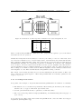
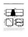
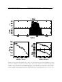
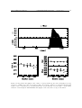
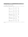
1
EUROPEAN SOUTHERN OBSERVATORY
Organisation Européene pour des Recherches Astronomiques dans l’Hémisphère Austral
Europäische Organisation für astronomische Forschung in der südlichen Hemisphäre
ESO - European Southern Observatory
Karl-Schwarzschild Str. 2, D-85748 Garching bei München
Very Large Telescope
Paranal Science Operations
OmegaCAM User Manual
Doc. No. VST-MAN-OCM-23110-3110
Issue 95.0, Date 27/08/2014
G. Beccari, S. Mieske, OmegaCAM consortium
Prepared
. . . . . . . . . . . . . . . . . . . . . . . . . . . . . . . . . . . . . . . . . .
Date
Signature
A. Kaufer
Approved
. . . . . . . . . . . . . . . . . . . . . . . . . . . . . . . . . . . . . . . . . .
Date
Signature
C. Dumas
Released
. . . . . . . . . . . . . . . . . . . . . . . . . . . . . . . . . . . . . . . . . .
Date
Signature
OmegaCAM User Manual
VST-MAN-OCM-23110-3110
This page was intentionally left blank
version 95.0
i
OmegaCAM User Manual
VST-MAN-OCM-23110-3110
version 95.0
ii
Document Change Record
Issue
Date
1.0
1.1
2.0 draft
31.03.2004
13.05.2004
20.12.2006
2.5
2.6
2.7
2.7.1.
3.0.
26.06.2011
11.08.2011
05.09.2011
14.09.2011
20.12.2011
90.0
27.02.2012
Sects. 3.4.1 & 3.7.1
90.1
91.0
92.0
92.1
95.0
24.05.2012
15.12.2012
07.03.2013
23.05.2013
23.08.2014
Sects. 3.4.4
Sect. 3.7.5.
Sect. 3.4.4.
Sect. 3.4.4.
Sect. 2.9.1.
Sect. / Paragr.
affected
all
most
Appendix
2.3
many, note 3.2.2 and 3.4.4
most
Reasons / Remarks
first issue (PAE)
changes in response to first RIXes (DBA, RHA)
small textual changes
Laboratory measurements of filter throughput
update based on commissioning
updates on filter naming and characteristics
Update by ESO-PSO after science verification
Minor language updates by ESO-USD
Update based on commissioning reports
and start of survey operations
Manual officially taken over by ESO
Update to overheads and PSF
Version number aligned with Period number
Update to overheads: IAstar and telescope offset
New Section 3.7.5. about vignetting by wind mast
Update to overheads: parallelised readout and preset/filter-set
Update to overheads: first offset in a template is 5s shorter
Performances of the new Baffling system installed in P94
OmegaCAM User Manual
VST-MAN-OCM-23110-3110
version 95.0
iii
Contents
1 Introduction
1
1.1
Credits . . . . . . . . . . . . . . . . . . . . . . . . . . . . . . . . . . . . . . . . . . . . .
1
1.2
Scope . . . . . . . . . . . . . . . . . . . . . . . . . . . . . . . . . . . . . . . . . . . . .
1
1.3
More Info . . . . . . . . . . . . . . . . . . . . . . . . . . . . . . . . . . . . . . . . . . .
1
1.4
References . . . . . . . . . . . . . . . . . . . . . . . . . . . . . . . . . . . . . . . . . . .
1
1.5
Acronyms . . . . . . . . . . . . . . . . . . . . . . . . . . . . . . . . . . . . . . . . . . .
2
2 Instrument characteristics
3
2.1
Overview . . . . . . . . . . . . . . . . . . . . . . . . . . . . . . . . . . . . . . . . . . .
3
2.2
Detector Mosaic . . . . . . . . . . . . . . . . . . . . . . . . . . . . . . . . . . . . . . .
7
2.2.1
The 268-Million Pixel Science Array . . . . . . . . . . . . . . . . . . . . . . . .
7
2.2.2
Auxiliary CCDs
. . . . . . . . . . . . . . . . . . . . . . . . . . . . . . . . . . .
13
Filters . . . . . . . . . . . . . . . . . . . . . . . . . . . . . . . . . . . . . . . . . . . . .
13
2.3.1
Note on filter magazines . . . . . . . . . . . . . . . . . . . . . . . . . . . . . . .
15
2.3.2
Providing Private Filters
. . . . . . . . . . . . . . . . . . . . . . . . . . . . . .
17
2.4
Shutter . . . . . . . . . . . . . . . . . . . . . . . . . . . . . . . . . . . . . . . . . . . .
18
2.5
Auto-Guiding and Focussing . . . . . . . . . . . . . . . . . . . . . . . . . . . . . . . . .
19
2.5.1
VST Guide Probe . . . . . . . . . . . . . . . . . . . . . . . . . . . . . . . . . .
19
2.5.2
Auto-guiding with OmegaCAM . . . . . . . . . . . . . . . . . . . . . . . . . . .
19
2.5.3
Differential Guiding . . . . . . . . . . . . . . . . . . . . . . . . . . . . . . . . .
19
2.5.4
Image Analysis with OmegaCAM . . . . . . . . . . . . . . . . . . . . . . . . . .
20
2.5.5
Traffic rules between science and auxiliary CCD readouts . . . . . . . . . . . .
20
2.6
Calibration lamps . . . . . . . . . . . . . . . . . . . . . . . . . . . . . . . . . . . . . . .
20
2.7
Photometric Properties . . . . . . . . . . . . . . . . . . . . . . . . . . . . . . . . . . .
21
2.8
Astrometric Properties . . . . . . . . . . . . . . . . . . . . . . . . . . . . . . . . . . . .
21
2.9
Flat fielding of OmegaCAM data / Illumination correction . . . . . . . . . . . . . . . .
21
2.9.1
22
2.3
Performances of the new Baffling system . . . . . . . . . . . . . . . . . . . . . .
3 Observing with OmegaCAM
3.1
22
Offsetting Modes and Observing Strategies . . . . . . . . . . . . . . . . . . . . . . . .
25
3.1.1
Offsetting Modes . . . . . . . . . . . . . . . . . . . . . . . . . . . . . . . . . . .
25
3.1.2
Observing Strategies . . . . . . . . . . . . . . . . . . . . . . . . . . . . . . . . .
26
OmegaCAM User Manual
3.2
VST-MAN-OCM-23110-3110
version 95.0
iv
Atmospheric Refraction and Dispersion . . . . . . . . . . . . . . . . . . . . . . . . . .
26
3.2.1
Atmospheric Refraction . . . . . . . . . . . . . . . . . . . . . . . . . . . . . . .
27
3.2.2
Atmospheric Dispersion . . . . . . . . . . . . . . . . . . . . . . . . . . . . . . .
27
OB preparation . . . . . . . . . . . . . . . . . . . . . . . . . . . . . . . . . . . . . . . .
29
3.3.1
Target acquisition . . . . . . . . . . . . . . . . . . . . . . . . . . . . . . . . . .
29
3.3.2
Scientific exposure . . . . . . . . . . . . . . . . . . . . . . . . . . . . . . . . . .
29
3.3.3
Dither and jitter patterns . . . . . . . . . . . . . . . . . . . . . . . . . . . . . .
29
The Observing templates . . . . . . . . . . . . . . . . . . . . . . . . . . . . . . . . . .
29
3.4.1
Target Acquisition Templates . . . . . . . . . . . . . . . . . . . . . . . . . . . .
29
3.4.2
Science Templates . . . . . . . . . . . . . . . . . . . . . . . . . . . . . . . . . .
30
3.4.3
Nighttime Calibration . . . . . . . . . . . . . . . . . . . . . . . . . . . . . . . .
31
3.4.4
Overheads . . . . . . . . . . . . . . . . . . . . . . . . . . . . . . . . . . . . . . .
31
3.5
Survey Area Definition Tool . . . . . . . . . . . . . . . . . . . . . . . . . . . . . . . . .
32
3.6
Selecting exposure times and number of sub-exposures . . . . . . . . . . . . . . . . . .
33
3.7
Special features of the data . . . . . . . . . . . . . . . . . . . . . . . . . . . . . . . . .
33
3.7.1
Point Spread Function . . . . . . . . . . . . . . . . . . . . . . . . . . . . . . . .
33
3.7.2
CCD blemishes and particle hits . . . . . . . . . . . . . . . . . . . . . . . . . .
34
3.7.3
Ghosts and reflections . . . . . . . . . . . . . . . . . . . . . . . . . . . . . . . .
34
3.7.4
Sky concentration . . . . . . . . . . . . . . . . . . . . . . . . . . . . . . . . . .
35
3.7.5
Vignetting close to wind mast position . . . . . . . . . . . . . . . . . . . . . . .
35
3.7.6
Diffraction Spikes . . . . . . . . . . . . . . . . . . . . . . . . . . . . . . . . . . .
38
3.7.7
Fringes . . . . . . . . . . . . . . . . . . . . . . . . . . . . . . . . . . . . . . . .
38
3.7.8
Remanence . . . . . . . . . . . . . . . . . . . . . . . . . . . . . . . . . . . . . .
38
3.7.9
CCD Crosstalk . . . . . . . . . . . . . . . . . . . . . . . . . . . . . . . . . . . .
39
3.3
3.4
4 Calibrating and Reducing OmegaCAM data
41
4.1
Calibration Plan . . . . . . . . . . . . . . . . . . . . . . . . . . . . . . . . . . . . . . .
41
4.2
Data reduction Pipeline . . . . . . . . . . . . . . . . . . . . . . . . . . . . . . . . . . .
43
4.3
Quality Control . . . . . . . . . . . . . . . . . . . . . . . . . . . . . . . . . . . . . . . .
44
A Filter throughput curves
45
A.1 Broad band Sloan filters (u′ g ′ r′ i′ z ′ ) . . . . . . . . . . . . . . . . . . . . . . . . . . . . .
45
A.2 Segmented Broad-band filters (Johnson B and V) . . . . . . . . . . . . . . . . . . . . .
51
A.3 Narrow-band filters (Strömgren v and Hα) . . . . . . . . . . . . . . . . . . . . . . . . .
51
OmegaCAM User Manual
VST-MAN-OCM-23110-3110
version 95.0
A.4 Radial variations in bandpass . . . . . . . . . . . . . . . . . . . . . . . . . . . . . . . .
B Detector response curves
v
52
53
List of Tables
1
Basic CCD characteristics . . . . . . . . . . . . . . . . . . . . . . . . . . . . . . . . . .
9
2
Properties of all 32 CCDs . . . . . . . . . . . . . . . . . . . . . . . . . . . . . . . . . .
13
3
Filters available in OmegaCAM . . . . . . . . . . . . . . . . . . . . . . . . . . . . . . .
16
4
Current OmegaCAM filter distribution. The opaque filter is required to protect the
instrument when it is not in operation. . . . . . . . . . . . . . . . . . . . . . . . . . . .
17
5
Magnitude zero points for the SDSS filter set. . . . . . . . . . . . . . . . . . . . . . . .
21
6
Illumination correction functions . . . . . . . . . . . . . . . . . . . . . . . . . . . . . .
22
7
Key difference between the dither and jitter modes. . . . . . . . . . . . . . . . . . . . .
26
8
Maximum airmasses without using the ADC . . . . . . . . . . . . . . . . . . . . . . . .
28
9
Overhead times for observations . . . . . . . . . . . . . . . . . . . . . . . . . . . . . . .
32
10
OmegaCAM Photometric Standard Star Fields . . . . . . . . . . . . . . . . . . . . . .
43
List of Figures
1
Schematic drawing of OmegaCAM . . . . . . . . . . . . . . . . . . . . . . . . . . . . .
3
2
Optical layout of the VST . . . . . . . . . . . . . . . . . . . . . . . . . . . . . . . . . .
4
3
Layout of the CCDs in the focal plane . . . . . . . . . . . . . . . . . . . . . . . . . . .
5
4
Spot Diagrams . . . . . . . . . . . . . . . . . . . . . . . . . . . . . . . . . . . . . . . .
6
5
Photograph of the detector mosaic . . . . . . . . . . . . . . . . . . . . . . . . . . . . .
8
6
Single CCD pixel layout . . . . . . . . . . . . . . . . . . . . . . . . . . . . . . . . . . .
10
7
Schematic of CCD readout . . . . . . . . . . . . . . . . . . . . . . . . . . . . . . . . .
11
8
Linearity of the CCDs . . . . . . . . . . . . . . . . . . . . . . . . . . . . . . . . . . . .
12
9
Filter times CCD throughput . . . . . . . . . . . . . . . . . . . . . . . . . . . . . . . .
14
10
An OmegaCAM filter . . . . . . . . . . . . . . . . . . . . . . . . . . . . . . . . . . . .
15
11
Shadow cast by the cross in composite filters . . . . . . . . . . . . . . . . . . . . . . .
16
12
Orientation of filter as function of magazine . . . . . . . . . . . . . . . . . . . . . . . .
17
13
The shutter unit . . . . . . . . . . . . . . . . . . . . . . . . . . . . . . . . . . . . . . .
18
14
Illumination correction derivation for OmegaCAM Sloan r . . . . . . . . . . . . . . . .
23
15
Asymmetric straylight in flatfields for OmegaCAM Sloan r . . . . . . . . . . . . . . . .
24
OmegaCAM User Manual
VST-MAN-OCM-23110-3110
version 95.0
vi
16
Raw dome flat divided by raw twilight flat for OmegaCAM Sloan r . . . . . . . . . . .
25
17
Limit on exposure time due to atmospheric refraction . . . . . . . . . . . . . . . . . .
28
18
OmegaCAM PSF anisotropies . . . . . . . . . . . . . . . . . . . . . . . . . . . . . . . .
33
19
OmegaCAM IQ distribution, collected between August and December 2011 . . . . . .
34
20
Example ghost reflection . . . . . . . . . . . . . . . . . . . . . . . . . . . . . . . . . . .
36
21
Reflection from a star outside the field . . . . . . . . . . . . . . . . . . . . . . . . . . .
37
22
Vignetting by wind mast . . . . . . . . . . . . . . . . . . . . . . . . . . . . . . . . . . .
37
23
Fringe maps in i′ and z ′ band . . . . . . . . . . . . . . . . . . . . . . . . . . . . . . . .
38
24
Crosstalk between CCDs 93–96 . . . . . . . . . . . . . . . . . . . . . . . . . . . . . . .
40
25
Frequency of calibration observations . . . . . . . . . . . . . . . . . . . . . . . . . . . .
42
26
Filter measurement location and coordinate system . . . . . . . . . . . . . . . . . . . .
45
27
u′ filter throughput . . . . . . . . . . . . . . . . . . . . . . . . . . . . . . . . . . . . . .
46
28
g ′ filter throughput . . . . . . . . . . . . . . . . . . . . . . . . . . . . . . . . . . . . . .
47
29
r′ filter throughput . . . . . . . . . . . . . . . . . . . . . . . . . . . . . . . . . . . . . .
48
30
i′ filter throughput . . . . . . . . . . . . . . . . . . . . . . . . . . . . . . . . . . . . . .
49
31
z ′ filter throughput . . . . . . . . . . . . . . . . . . . . . . . . . . . . . . . . . . . . . .
50
32
CCD Quantum efficiency curves . . . . . . . . . . . . . . . . . . . . . . . . . . . . . . .
53
OmegaCAM User Manual
1
1.1
VST-MAN-OCM-23110-3110
version 95.0
1
Introduction
Credits
This manual is largely based on the OmegaCAM user manual drafted and maintained by the OmegaCAM consortium (Konrad Kuijken, Bernard Muschielok, Andrea Baruffolo) between 2004 and 2011
until end of OmegaCAM commissioning. It also includes content from the OmegaCAM DFS Commissioning Reports, and input from the OmegaCAM IOT. It will be updated continously by Paranal
Science Operations, as survey operations evolve and more experience is gathered.
1.2
Scope
OmegaCAM is the wide-field imager for the Cassegrain focus of the VLT Survey Telescope (VST) on
Paranal, a 2.6m modified Richie-Chretien alt-az telescope designed specifically for wide-field imaging.
It is the only instrument on this telescope, and is operated most nights. In principle all observations
are carried out in service mode. Its main function is to perform large optical imaging surveys, which
may be used to feed the VLT telescopes with targets. With its wide field, broad-band filter set, and
image quality matched to Paranal seeing conditions, OmegaCAM is well-suited to this task.
This document serves as a user manual for those planning or preparing observations with OmegaCAM.
It describes the main instrument characteristics, and how to observe with it using Observation Blocks
and Observing Templates.
The most recent version of this manual is kept at
http://www.eso.org/sci/facilities/paranal/instruments/omegacam/doc/.
1.3
More Info
Further information can be obtained by contacting [email protected] and consulting the public
OmegaCAM webpage http://www.eso.org/sci/facilities/paranal/instruments/omegacam/. ESO
Quality Control Pages are found at http://www.eso.org/observing/dfo/quality/ALL
1.4
References
[RD1] Template Manual, VST-MAN-OCM-23100-3111,
see http://www.eso.org/sci/facilities/paranal/instruments/omegacam/doc/.
[RD2] Calibration Plan, VST-PLA-OCM-23100-3090,
see http://www.eso.org/sci/facilities/paranal/instruments/omegacam/doc/.
[RD3] DFS User Requirements, VST-SPE-OCM-23100-3050,
see http://www.eso.org/sci/facilities/paranal/instruments/omegacam/doc/.
[RD4] WFI documentation, see http://www.ls.eso.org/lasilla/sciops/2p2/E2p2M/WFI/.
[RD5] P2PP instructions, see http://www.eso.org/sci/observing/phase2/P2PPSurveys.html/.
[RD6] OmegaCAM public webpage, see http://www.eso.org/sci/facilities/paranal/instruments/omegacam/.
[RD7] ESO QC web page, see http://www.eso.org/observing/dfo/quality/ALL/
OmegaCAM User Manual
1.5
VST-MAN-OCM-23110-3110
version 95.0
2
Acronyms
ADC: Atmospheric dispersion compensator, a device which corrects for the chromatic effects of the
atmosphere at low elevations.
CCD: Charge-couple device, a solid-state, panoramic light detector of high quantum efficiency.
CTE: Charge Transfer Efficiency. The efficiency of the charge transport during readout.
DFS: Data Flow System.
DIMM: Differential Image Motion Monitor
e2v: Manufacturer of the OmegaCAM CCDs.
ETC: Exposure Time Calculator, a software tool provided by ESO as an aid in planning observations.
FOV: Field-of-view
FWHM: Full Width at Half-Maximum.
IQ: Image Quality
MPG: Max Planck Gesellschaft.
OB: Observation Block, a set of instructions to telescope and instrument to carry out a specific
observation.
OmegaCAM: The wide-field CCD camera for the VST.
P2PP: Phase 2 Proposal Preparation, the process at ESO in which the users define the OBs for their
approved programmes by means of special software.
PA: Position Angle, orientation of the field of view on the sky. For VST/OmegaCAM, PA=0 means
that North is in positive y-direction and East is in negative x-direction.
PSF: Point-Spread-Function
RMS: Root-mean square.
SADT: Survey Area Definition Tool
SDSS: Sloan Digital Sky Survey, a large imaging and spectroscopy survey of (mostly) the Northern
hemisphere. OmegaCAM’s science filter set include the five SDSS filters u′ g ′ r′ i′ z ′ .
USM: Universitätssternwarte München
USNO: US Naval Observatory. Their all-sky catalogue is used for astrometric calibration of OmegaCAM data.
VLT: Very Large Telescope, four 8m telescopes on ESO’s Paranal Observatory.
VST: VLT Survey Telescope, a 2.6m telescope at ESO’s Paranal Observatory dedicated to optical
surveys, and host to OmegaCAM.
WFI: Wide-Field Imager, an 8-CCD mosaic camera on the ESO/MPG 2.2 telescope on La Silla with
similar pixel scale and sensitivity to OmegaCAM.
OmegaCAM User Manual
VST-MAN-OCM-23110-3110
version 95.0
3
Figure 1: Schematic view of the instrument. Key components are labelled.
2
2.1
Instrument characteristics
Overview
OmegaCAM (see Fig. 1) is the wide-field imager for the Cassegrain focus of the VLT Survey Telescope
(VST) on Paranal, a 2.6m modified Richie-Chretien alt-az telescope designed specifically for wide-field
imaging. It is the only instrument on this telescope, and is operated most nights. In principle all
observations are carried out in service mode.
The VST/OmegaCAM system is designed for good seeing-limited image quality over a wide field. The
telescope has an actively controlled meniscus primary mirror, an active secondary, and an image analysis system. It contains two interchangeable correctors: one is a high-throughput two-lens corrector
which works in u′ -z ′ bands, the other contains an Atmospheric Dispersion Compensator (ADC) for
work at lower elevations. The ADC has almost no throughput in the u′ band.
The optical layout of the VST is illustrated in Fig. 2.
The VST provides a 1 degree unvignetted field of view, which OmegaCAM samples with a 32-CCD,
16k x 16k detector mosaic (Fig. 3) at 0.21 arcsec per pixel (0.213 for the two-lens corrector, 0.215
for the ADC configuration). Each CCD is of 2k x 4k format and subtends ∼ 7.3′ × 14.6′ on the sky.
The CCDs are thinned, blue-sensitive, 3-edge buttable CCD44-82 devices from e2v of high (but not
perfect) cosmetic quality. Image quality is specified such that in the absence of seeing 80% of the
energy from a point source should fall within a 2x2 pixel area over the full field (see example spot
diagrams in Fig 4). The field distortion is very low, so that the image scale is virtually constant over
the whole field. There are narrow gaps between the CCDs: the overall geometric filling factor of the
array is 91.4%.
In addition to the 32 CCDs making up the science array, OmegaCAM also contains four auxiliary
CCDs around the edges of the field. Two of these are used for autoguiding, so that both field position
OmegaCAM User Manual
VST-MAN-OCM-23110-3110
version 95.0
4
Figure 2: Optical layout and selected light paths through the VST. The configuration with the twolens corrector is shown. The bottom panel shows a zoom onto the corrector optics: the incoming light
passes through two spherical lenses, a planar filter, and the spherical dewar entrance window before
reaching the CCDs on the right. Scales are in mm.
OmegaCAM User Manual
VST-MAN-OCM-23110-3110
version 95.0
5
Figure 3: The layout of the 32 science CCDs and the four auxiliary CCDs in the focal plane. The
science array covers a 1 degree x 1 degree area of sky, with 16k x 16k pixels of 0.21 arcsec. All CCDs
fit inside a circle of diameter 1.4 degrees on the sky. (Note that this is the layout as seen from below,
i.e., the projection of the array onto the sky.)
OmegaCAM data are delivered as multi-extension FITS files. The CCD name (#65–96) is included in
the header of each fits extension. CCDs can also be identified by the number of their fits extension, but
beware: this order may change from what is shown in the Figure whenever CCD controller parameters
are changed.
Two of the auxiliary CCDs are mounted out of the focal plane (Extra- and Intra-focal; IF & EF),
at displacements ±2mm, in order to enable image analysis and real-time active optics corrections.
Auxiliary CCDs G1 and G2 are used for guiding. All 4 auxiliary CCDs are partly vignetted around
their respective outermost corner.
OmegaCAM User Manual
VST-MAN-OCM-23110-3110
version 95.0
6
Figure 4: Sample spot diagrams for 500nm light in a quadrant of the OmegaCAM focal plane. A 2x2
pixel grid (30µm × 30µm, corresponding to 0.43′′ ) is shown as well.
OmegaCAM User Manual
VST-MAN-OCM-23110-3110
version 95.0
7
and rotation can be tracked accurately. The other two auxiliary CCDs are mounted 2mm outside the
focal plane (one in front, one behind), and are used for recording defocused star images for on-line
analysis of the image quality. The CCD layout in the focal plane is shown in Fig. 3. A photograph of
the detector mosaic is shown in Fig. 5.
OmegaCAM contains a 12-slot filter exchange mechanism, subdivided into two cabinets of six slots
each. Currently the available filters include the Sloan u′ g ′ r′ i′ z ′ set, Johnson B and V filters, several
narrow-band filter mosaics, a Strömgren v filter, and a special calibration filter (see Table 3).
OmegaCAM data are taken in the context of a calibration plan [RD2] that ensures that all data can
be photometrically and astrometrically calibrated to 0.05 magnitudes and 0.1 arcsec rms precision,
respectively. See Sect. 4.1.
Compared to the wide-field imager (WFI [RD4]) on the ESO/MPG La Silla 2.2m telescope, OmegaCAM on the VST offers
1. a four times larger field
2. better cosmetic quality CCDs
3. a primary mirror of 1.4 times the area
4. year-round operation in service mode
5. better image quality due to active telescope optics, astro-climate
6. the Sloan filter set (but only very few narrow-band filters)
2.2
2.2.1
Detector Mosaic
The 268-Million Pixel Science Array
The central 32 CCDs of OmegaCAM form the science array, the heart of the instrument. Basic
characteristics of the CCDs are found in Table 1. Consult also the OmegaCAM QC webpages [RD7]
for up-to-date information. The CCD type is e2v, CCD44-82.
The packaging of a single CCD is illustrated in Fig. 6. The light-sensitive area consists of 4100x2048
pixels, surrounded by a border whose width is 0.16mm on the short side opposite the readout register,
0.5mm along the long sides of the CCD, and 5mm on the side of the readout register. Unavoidably
therefore, there are small ’dead zone’ gaps in the science array between the light-sensitive areas of
neighbouring CCDs. How the CCDs are mounted together in the array is indicated in Figs. 3 and 5.
The CCDs are mounted as closely as possible. The resulting average gap sizes are:
• between the long sides of the CCDs: 1.5mm (100 pix=21.5′′ )
• central gap along the short sides: 0.82mm (55 pix=11.8′′ )
• wide gap along short sides: 5.64mm (376 pix=80.5′′)
• between science array and auxiliary CCDs: 15.9mm (1060 pix)
All CCDs are read out at 280kpix/s, through one amplifier port each (in all cases situated at the
”left” end of the readout register). The resulting image comes with 48 columns of pre- and overscan,
and 100 rows of vertical overscan. Because of their construction and the way they are arranged in
the mosaic, all CCDs are read out along their long side, in a direction away from the center of the
mosaic. In the lower half of the CCD array, the readout register is at the ”bottom” (southern edge)
of the CCDs, whereas in the upper (northern) half the CCDs are rotated through 180 degrees.
OmegaCAM User Manual
VST-MAN-OCM-23110-3110
version 95.0
8
Figure 5: Picture of the 36 CCDs mounted behind the dewar window. Note the black strips that
cover the gaps between the CCDs: they prevent reflection of light off the bright bond wires of each
detector. Slight vignetting is observed near these strips, and on the long outer sides of the four corner
CCDs.
OmegaCAM User Manual
CCD Parameter
CCD type
Pixel size
Format
Default Read Speed
Flatness
R.O.N.
(not including system noise)
Full R.O.N.
(including system noise)
at default read speed
Gain [e-/ADU]
Output Amplifiers
Device Layout
Dump Drain
Cosmetics
CTE
Horizontal Transfer Frequency
Vertical Transfer Frequency
Full Well / Linearity
Dark Current
Cross talk
Gain variations
Cosmic Ray Sensitivity
Optical Coating
Package design
VST-MAN-OCM-23110-3110
version 95.0
9
Value
Marconi / e2v / CCD 44 - 82 - 1 - A57
thin devices (20µm)
15 µm
Active Pixel Area 2048 x 4102 pixels (2048x4100 used)
50 horizontal pre- and 50 overscan pixels
280 kpix/sec
< 20µm peak to valley
2 e- at 50 kpix/sec
4 e- at 500 kpix/sec
6 e- at 1000 kpix/sec
5-7 e∼2.6 with 10% chip-to-chip RMS
2 identical output amplifiers with integrated post chip amplifiers.
Charge can in principle be read through either one completely
or through both of them simultaneously. In practise,
only the respective ”left” one is used.
No frame transfer option, 3 phase parallel register (non split),
3 phase serial register (split)
A dump drain exists parallel to the serial readout register,
so that lines can be discarded as a whole
A global defect budget exists, specifying the overall defects
for all of the 40 science devices
(Cosmetically the final device cosmetics are much better than
devices used for the WFI)
> 0.999995 per parallel or serial shift
2 Mpixels/sec
15-20 klines/sec
>200 000 e-.
Serial full well is at least 2 times the pixel full well and the summing
full well is at least 4 times the pixel full well. These full well values
correspond to the maximum charge that can be handled while attaining
the CTE specified. Amplifier full well is around 200 000 e-. Amplifier
full well refers to the limit of linearity, i.e. the maximum amount of charge
that can be amplified while producing output that matches a linear response
to within 1 %.
< 2 e- / pixel / hour (at operating temperature of −120 o C)
There is cross talk at the level of < 0.4% between CCDs 93-96.
CCDs # 87 and 88 shows day-to-day gain variations of 1-2% RMS.
< 3 events / square cm and minute
Single layer anti reflection coating astro BB
(with thickness 42nm instead of 46nm)
Four side buttable (fourth side with larger gap),
Invar package with integrated PT100 temperature sensor
Table 1: Basic characteristics of the OmegaCAM CCDs. See also Table 2 and Fig. 8.
OmegaCAM User Manual
VST-MAN-OCM-23110-3110
version 95.0
10
Figure 6: The light-sensitive area of a single CCD. Units are in mm, size of a single pixel is 15 µ.
The readout seqence is illustrated in Fig. 7. The science mosaic is read out by two FIERA systems, one
for each half (East/West) of the array. Total readout time is 29sec. Combined with other overheads,
principally the time needed to wipe the array before a new exposure, this leads to a total minimum
shutter-closed time between successive exposures of 40 seconds.
Generally the CCDs in the array are similar, but they do differ in detail. A number of properties of
the CCDs are tabulated in Table 2, in a format that corresponds to their layout in the science array
(top view). At the default sky position angle of zero degrees this layout corresponds to N at the top,
and East to the right.
Complete QE curves for each of the CCDs are given in Appendix B.
All CCDs but three have parallel and serial CTE above 0.999995, the exceptions being:
• CCD #65 and #96, which have serial CTE 0.999994
• CCD #72 which has serial CTE 0.999993
With a gain of ca. 2.6 electrons per ADU, the analog-to-digital conversion of the amplifier output of
each CCD saturates before the CCD full-well capacity of over 200.000 electrons. Below this saturation
the response of the CCDs is linear to within 1%, as can be seen from Fig. 8.
The flat fields of the CCDs show different behaviour, dependent on the wavelength. In the u′ band,
the flat fields show a diagonal, diamond-like pattern, which is caused by the thinning process. A
few of the CCDs (#65, 66, 86, 87) also show an ’ink pattern’, areas of very high UV sensitivity (the
origin of this feature is unknown). At intermediate wavelengths (g ′ , r′ ) the flat fields are reasonably
featureless. At longer wavelengths (i′ and particularly z ′ ), fringing occurs, leading to swirling patterns
reminiscent of a thin film of oil on water. All artifacts can be removed in data reduction.
The efficiency of the filters, folded with the detector response, is plotted in Fig. 9. Detailed analysis
of the filter throughput, including bandpass variations across the fields, is deferred to Appendix A.
See Sect. 3.7 for a description of particular features that occur in scientific data obtained with Omega-
OmegaCAM User Manual
VST-MAN-OCM-23110-3110
version 95.0
Figure 7: Data flow diagram for readout of the OmegaCAM science array.
11
OmegaCAM User Manual
VST-MAN-OCM-23110-3110
version 95.0
12
Figure 8: Plot of the linearity of the response of each CCD, as a function of illumination level.
(Obtained by exposing the mosaic to a calibration lamp, with varying exposure times).
OmegaCAM User Manual
VST-MAN-OCM-23110-3110
13
version 95.0
Table 2: Properties of all 32 CCDs
N (at PA 0 degrees)
CCD number
gain (e-/ADU)
readnoise (e-)
# hot pixels
# cold pixels
dark current (ADU/hr)
#89
2.37
6.52
50
3143
0.50
#81
2.57
5.20
25
8698
0.36
#73
2.40
4.70
7
3811
0.35
#65
2.39
4.73
7
2807
0.30
#90
2.52
6.23
14
16719
0.46
#82
2.56
5.05
3490
2816
0.28
#74
2.48
5.18
16
2692
0.22
#66
2.59
5.10
131
5363
0.36
#91
2.62
5.98
11
8891
0.36
#83
2.56
5.22
28
9611
0.41
#75
2.52
5.12
18
2765
0.21
#67
2.49
5.20
25
2956
0.26
#92
2.56
6.03
24
4926
0.47
#84
2.46
5.06
825
5713
0.31
#76
2.44
4.97
20
2802
0.28
#68
2.55
5.42
109
4163
0.30
#93
2.56
5.15
18
7037
0.27
#85
2.40
5.19
11
9742
0.33
#77
2.66
5.95
13
2683
0.33
#69
2.48
5.28
18
3003
0.25
#94
2.78
5.61
16
15038
0.37
#86
2.32
4.82
13
6420
0.40
#78
2.71
5.31
7
2660
0.26
#70
2.23
4.69
20
5783
0.31
#95
2.73
6.90
17
10134
0.15
#87
2.39
5.10
19
8570
0.37
#79
2.67
5.36
58
2911
0.24
#71
2.54
5.08
16
7371
0.27
#96
2.37
5.17
18
7222
0.34
#88
2.52
5.22
9
9553
0.38
#80
2.57
5.17
50
4329
0.29
#72
2.39
4.83
13
4191
0.28
E
CAM, many of which follow from the properties of the detectors.
2.2.2
Auxiliary CCDs
In the periphery of the focal plane OmegaCAM contains four auxiliary CCDs. Two of these are used
for guiding (called G1 and G2), both in position and position angle of the field. The other two are
mounted out of focus (one is 2mm in front of the focal plane, one 2mm behind). Analysis of pairs of
defocused images from these CCDs allows optical aberrations (defocus, coma, astigmatism, ...) to be
measured and the telescope to be kept in focus.
2.3
Filters
The filter exchange mechanism (Fig. 10) selects filters from two magazines located either side of the
focal plane inside the instrument, and slides these into the beam. Each magazine can store six filters.
Filter positioning is repeatable to very high accuracy resulting in less than 0.3% rms flux variations
between flat fields taken at different times. The footprint of a stellar image is about 1cm in size.
The available filters are listed in Table 3. Transmission curves as measured in the lab are included in
Appendix A.
The filters are sandwiches of glass substrates, ca. 14mm thick. Each filter has a baseplate (usually
made of BK7) which provides the mechanical support and mounting to the filter frame. Further layers
of glass are glued onto this base plate, and provide the filter bandpass, either through coating or by
means of coloured glass. For the segmented filters B, V, and NB 659, these layers consist of four
quadrants, and the interface of the quadrants casts a slight shadow in the form of a cross onto the
OmegaCAM User Manual
VST-MAN-OCM-23110-3110
version 95.0
14
Figure 9: Throughput of the OmegaCAM Sloan filters, times the average quantum efficiency of the
CCDs. For comparison, standard (normalised) Johnson-Cousins UBVRI filters are also shown.
OmegaCAM User Manual
VST-MAN-OCM-23110-3110
version 95.0
15
Figure 10: A single OmegaCAM filter ready to be loaded into the instrument. Note the separate
filters covering the auxiliary CCDs.
image plane (Fig. 11). This central vignetting cross covers ±310′′ in X and Y direction. In a science
observation (Sect. 3.1.1) it can therefore be dithered out with a dither amplitude of 310′′ in both X
and Y.
Most of the narrow-band filters consist of quadrants where each quadrant has a different bandpass.
By offsetting the telescope in half-degree steps, and/or rotating the instrument through multiples of
90 degrees, the full field of view can be exposed in all four bandpasses. Which CCD was exposed with
which filter segment depends on the magazine the filter is loaded in - this is recorded in the image
FITS header (see below, Note on filter magazines).
The auxiliary CCDs, used for guiding and image analysis, are covered by separate filters. Usually
these have nearly the same bandpass as the main science filter, but in some cases (the narrow band
filters and the u band filter) they are different, in order to boost sensitivity and increase the number
of guide stars that can be used.
The Calibration filter is used to observe standard star fields in four bands simultaneously, and hence
to monitor variations in the atmospheric extinction throughout the night. For this purpose a specially
calibrated standard star field near the South celestial pole has been established (see Sect. 4.1).
2.3.1
Note on filter magazines
Because the filter frames can only mate with the filter insertion mechanism on one side, the orientation
of a filter with respect to the CCD mosaic depends on the magazine in which it was stored (see Fig. 12).
During observations the filter exchange mechanism always returns a filter to the magazine (and slot
within that magazine) it came from. However, it may happen that a filter needs to be moved manually
from one magazine to the other during daytime operations. This flips the orientation of the filter by
180 degrees.
OmegaCAM User Manual
VST-MAN-OCM-23110-3110
version 95.0
16
Figure 11: The shadow cast by the cross that separates the different segments of a composite filter
(here the V filter).
Filter name
u′
g′
r′
i′
z′
B
V
v
Hαd VPHAS+
Hαe
Hα(z = 0.3)f
NB3f
NB4f
Calibg
System
SDSS
SDSS
SDSS
SDSS
SDSS
Johnson
Johnson
Strömgren
—
—
—
—
—
SDSS
Table 3: Filters available in OmegaCAM
λ (nm)a
∆λ (nm)b P2PP name
354
56
u SDSS
475
134
g SDSS
625
135
r SDSS
756
155
i SDSS
880
80
z SDSS
439
103
B JOHN
551
98
V JOHN
412
21
v STRM
658.6, 659.3
10.5
NB 659
659.0, 666.0, 672.6, 679.1
11
H ALPHA
851.9, 861.4, 869.0, 877.7
12.5
NB 852 861 869 878
453.6, 494.3, 533.5, 575.6
15–20
NB 454 494 533 575
616.1, 710.2, 755.1, 816.4
13–20
NB 617 710 755 817
u′ ,g ′ ,r′ ,i′
u g r i SDSS
commentc
IF, M
IF, M
IF, M
IF, M
IF, M
IF, S
IF, S
IF, M
IF, S
IF, 4Q
IF, CG, 4Q
IF, CG, 4Q
IF, CG, 4Q
IF, CG, 4Q
a
Central wavelength and b FWHM of filter throughput × mean CCD QE curve
IF=Interference Filter; CG=Coloured Glass filter; M=Monolithic; S=Segmented; 4Q=4 quadrants with different passband.
d
This is a private filter for the VPHAS+ survey. Note the slightly different central wavelength of one of the
segments.
e
Hα in four slightly overlapping redshift ranges: z = 0, 0.01, 0.02, 0.03.
f
These are private filters for use by Munich University Observatory for the first five years of OmegaCAM
operations. Note that these are not currently mounted.
g
Because of the different manufacturing processes, the Calib filter bandpasses differ in detail from the monolithic filters.
c
For the filters consisting of different quadrants, the layout of the quadrants on the sky is as shown
below when the filter is inserted in magazine A (for the default orientation of the instrument with
PA=0, North is up, East to the left). If the filter is mounted in magazine B the orientation is rotated
by 180 degrees.
Hα
679 673
659 666
Hα VPHAS+
658.6 658.6
659.3 658.6
Hα(z = 0.3)
852
869
861
878
NB3
494 454
533 576
NB4
710 616
816 755
Calib
u′ i′ .
g ′ r′
OmegaCAM User Manual
VST-MAN-OCM-23110-3110
version 95.0
17
Figure 12: Orientation of a filter depends on whether it is loaded in magazine A or B.
Magazine A
u
r
z
V
v
calib
Magazine B
opaque
g
i
B
Halpha
NB659
Table 4: Current OmegaCAM filter distribution. The opaque filter is required to protect the instrument when it is not in operation.
Manual filter manipulations should always be followed by the taking of a new set of flat fields, but if
for some reason old flats need to be used it is important to check that these were taken with the same
filter orientation. Which magazine a filter was loaded from is logged in the image headers (keyword
INS.FILT1.NO: magazine ‘A’ contains filter positions 1–6; magazine ‘B’ positions 7–12). Changing
from one filter to the next is faster when the filter is in the opposite magazine, since this allows to
perform parallel motions of both filters (inserting one, removing the other one). The typical time for
filter exchange is one minute for filters between different magazines, and two minutes for filters in the
same magazine. See also Table 9 which lists the OmegaCAM observing overheads.
The current order in which the filters are stored in the instrument is shown in Table 4. This order
tries to anticipate the typical sequence of filter changes within OBs. It is currently optimised for the
sequence u′ -g ′ -r′ -i′ -z ′ .
2.3.2
Providing Private Filters
It is possible, but not simple, to use private filters with OmegaCAM. There are a number of constraints:
1. The filters need to be mounted in special frames. These frames grab the filters by the baseplate,
which needs to be approx. 5mm thick. Spare frames exist.
2. Overall optical thickness should be equivalent to 15mm fused silica.
3. The costs of these large filters are high (50-100 kEuro), and manufacturing times long (up to a
year or more).
People interested in using private filters with OmegaCAM should contact the ESO User Support
Department ([email protected]).
OmegaCAM User Manual
VST-MAN-OCM-23110-3110
version 95.0
18
Figure 13: Picture of the partly disassembled shutter unit (Bonn shutter). The two blades, as well as
the central aperture, are visible in the lower part of the unit.
2.4
Shutter
The shutter of OmegaCAM is located on top of the instrument, in front of the filters. When closed it
covers all 36 CCDs (science + auxiliary). It is a low-acceleration, twin-blade photometric shutter of
aperture 370×292mm. The leading blade exposes the CCDs, the trailing blade covers them again. By
ensuring that both blades travel with the same acceleration profile the exposure is kept homogeneous
over the full beam. For very short exposures (below 0.8 s) the trailing blade starts its motion before
the leading blade has finished moving. Over the science CCDs the blades move at constant speed.
Even for exposures as short as 0.1 seconds, the homogeneity over the field is better than 1%. However,
it is important to realize that exposures are not simultaneous: there is a lag of about 0.5 second between
the exposures at the leading and trailing edge of the field. For high timing accuracy observations, the
delay time
tdelay = 0.39 + 0.00174X seconds
(1)
needs to be added to the absolute time of the exposure start and end. Here, X is in mm with respect
to the center of the detector mosaic (1mm=14.3 arcsec), and runs along the short sides of the CCDs
in the direction of motion of the blades.
The signs of the header keywords DET SHUT TMCLOS and DET SHUT TMOPEN record from
which direction the shutter was opened. After the initialisation/reset of the shutter it is always the
same blade that covers the mosaic, no matter what the previous state was. This blade is defined
as BLADE 1 and the blade outside the aperture as BLADE 2. BLADE 1 is at the +x side of the
instrument. For the first exposure in a new sequence, BLADE 1 will move outside the aperture and
after the exposure time BLADE 2 will move into the aperture. For the next exposure BLADE 2
will uncover the aperture and BLADE 1 moves in again after the exposure is over. The sign of the
header keywords are therefore related to the shutter motion in the following way: Blade 1 –> Blade
2 implies a positive value of DET.SHUT.TM keywords. Blade 2 –> Blade 1 implies a negative value
of DET.SHUT.TM keywords.
Note that the shutter blades are quite far from focus: at the shutter location the light from a given
star is smeared out over a width of about one tenth of the full shutter aperture. This means that the
time over which a given pixel receives photons is longer than the actual exposure time, by an amount
of roughly 0.08 s. Seen from an individual pixel the photon rate over time does not have steep edges
but is smeared out.
OmegaCAM User Manual
2.5
VST-MAN-OCM-23110-3110
version 95.0
19
Auto-Guiding and Focussing
Both the VST and OmegaCAM contain systems for auto-guiding and for focussing. Focussing happens
automatically through real-time sensing of the wavefront. (Filter-dependent focus offsets are also
automatically applied.) Traditional through-focus sequences are only needed to calibrate these autofocus systems.
The VST tracks well, and for exposures shorter than 60 sec there is no need to auto-guide. Depending
on the user’s image quality requirements, up to 2 minutes without guiding can be accepted, if the
target never approaches the zenith to closer than 10 degrees. Commissioning and verification tests
have shown that tracking drifts are of order ∼0.1-0.2” per minute, but increase when the telescope
approaches zenith. Whether autoguiding is desired or not can be specified in the acquisition template
of an Observation Block.
2.5.1
VST Guide Probe
The VST contains a guide probe with a pick-off mirror, which can patrol the field in front of the
filters. It can be used for guiding the telescope and for its active optics system. When required, the
probe can be used in between scientific exposures to measure the optical image quality by means of
a Shack-Hartmann analysis. This information can then be used to configure the telescope’s active
optics system.
The probe can in principle also be used for autoguiding and image analysis during scientific exposures.
However, unless a suitable guide star exists very close to the edge of the field, the probe vignets the
field of view. Use of the OmegaCAM guide and image analysis sensors is thus the default way of
operating OmegaCAM and VST. It also avoids the need to move the VST probe in and out of the
field, which takes several minutes.
2.5.2
Auto-guiding with OmegaCAM
Two guider CCDs are mounted diametrically opposite to each other, near the edges of the field (see
Fig. 3). Auto-guiding is done simultaneously on two stars, one on each guider CCD. Guiding with
two stars allows field center and rotation to be tracked during an exposure. When the shutter closes,
the guider CCDs are not exposed to the sky, and guiding cannot take place. Acquisition of the two
guide stars, one per CCD, is designed to happen automatically. If after a readout a second exposure
is taken of the same field, the guide stars are re-acquired once the shutter is reopened. If there was
no offset commanded for this new exposure, then the auto-guiding will attempt to return the guide
stars to the same pixels as in the previous exposures. If an offset is commanded, the auto-guiding will
simply keep the stars on the pixels where they are found in this new exposure (i.e., the system does
not calculate to which pixels the telescope offset should have sent the stars, but rather assumes that
the offset was applied correctly). Telescope offsets that are sufficiently small to keep the guide star
on its CCD are accurate to at worst 1 arcsec.
2.5.3
Differential Guiding
For observations where non-siderial pointing is required, e.g. to follow or search for solar system
objects, the telescope can be given a differential tracking rate. It is currently not possible to guide in
this mode, either with the VST guide probe or with OmegaCAM. Differential Guiding has not
been fully commissioned and is not offered for the observing periods P88 and later..
OmegaCAM User Manual
2.5.4
VST-MAN-OCM-23110-3110
version 95.0
20
Image Analysis with OmegaCAM
The other two auxiliary CCDs are mounted out of focus, see Figs. 3 and 5. They intersect the stellar
light beams in two planes, one in front of, and one behind, the focal plane. This gives information
on the deviation of the beams from perfect cones with apex in the focal plane. Different kinds of
aberration result in different shapes for these defocused stars, and this can be used to calculate
corrections to be applied to the VST’s active primary and secondary mirrors. Acquisition of the two
image analysis stars, one per CCD, is designed to happen automatically, as does the computation of
aberration coefficients. Image analysis is performed at the same wavelength as the autoguiding, which
in most cases is the same as the science filter (see Sect. 2.3).
Image Analysis in the aquisition typically requires 3 iterations of 40 seconds each. During science
exposures, aberrations are constantly measured by the IA system, and corrections are applied to
the mirrors during the readout. The minimum science integration time that guarantees at least one
aberration measurement is about 1 minute. OBs with shorter science exposures will not get additional
IA corrections after the aquisition. Tests have shown that the IQ remains reasonably stable for about
half an hour without IA corrections. OBs that consist of short integration times should therefore not
last more than half an hour. Image Analysis in the aquisition can be disabled for concatenations of
short OBs that perform a sequence of observations back-to-back in adjacent fields.
2.5.5
Traffic rules between science and auxiliary CCD readouts
The OmegaCAM CCDs are controlled by three controllers (called FIERA 1/2/3), where FIERAs 1
& 2 control the science CCDs, and FIERA 3 the auxiliary CCDs (Fig. 3). FIERA1 is the master
controller (Fig. 7). The readout rules are such that the science array cannot be read out at the same
time than the auxiliary CCDs. Otherwise, strong interference noise patterns will appear in auxiliary
and science CCDs. Therefore, the AG and IA loops always stop about 10 seconds before the end of
each science exposure.
Furthermore, upon science CCD readout, the OmegaCAM shutter is closed, such that no light falls
on the auxiliary CCDs either. AG and IA are therefore always paused from 10s before the end of a
science integration until the start of the next science integration.
2.6
Calibration lamps
Dome flat exposures are taken with calibration lamps mounted at 90◦ intervals on the top ring of the
telescope, illuminating a white screen on the inside of the telescope dome. The lamps are operated
by carefully controlling the electric current, and their brightness is stable to about a percent over a
timescale of several weeks.
Dome flat fields are used for monitoring the small-scale (pixel-to-pixel) variations in sensitivity of
OmegaCAM, and for overall system throughput monitoring. Two sets of four lamps each are mounted
side by side. One set is used for routine daily calibrations, meanwhile the second set is cross-calibrated
against the first at regular intervals. Once the lifetime of the first set of lamps has expired, its role
is taken over by the second set, and the first set is replaced with new lamps. This procedure ensures
a continuous record of throughput measurements, provides dome flat fields, and serves as a daytime
health check.
OmegaCAM User Manual
2.7
VST-MAN-OCM-23110-3110
version 95.0
21
Photometric Properties
Indicative magnitude zero points (the AB magnitude of a star that generates one electron per second)
are given in Table 5. These numbers are consistent with the on-line Exposure Time Calculator (ETC)1 ,
which is based on the throughputs and reflectivities of the individual optical components.
Because the angle of light incidence varies with distance from the center, the OmegaCAM filters show
some bandpass variation across the field. This variation is mostly axisymmetric, and it introduces a
radially dependent colour term. Measurements will be included once they are available.
Filter
u′
g′
r′
i′
z′
B
V
Mag zero pt (AB)
23.9
25.8
25.7
25.2
23.8
25.7
25.5
Table 5: Magnitude zero points for the SDSS and Johnson filter sets. These are average values;
chip-to-chip scatter is of order 0.1 mag.
2.8
Astrometric Properties
By design, OmegaCAM and the VST deliver a quite constant plate scale, and a rather uniform PSF.
The radial plate scale is constant over the field to better than 1 part in 1000, and independent of the
filter used. The pixel scale with ADC in is 0.215′′/pix. With the ADC out – hence two-lens corrector
in – it is 0.213′′ /pix.
2.9
Flat fielding of OmegaCAM data / Illumination correction
Both twilight (and to lesser extent dome flats) have a straylight component. This straylight component
is centrally concentrated (“sky concentration”) and makes the flatfield exposures overexposed in the
center of the FOV. Applying the flatfield exposures without any correction would result in an erroneous
apparent trend of photometric ZP with distance from FOV center. The sky concentration hence needs
to be corrected for, after flatfielding the data. The corresponding procedure is called Illumination
Correction (see e.g. Section 2.8.4. of McFarland et al. 2011, arXiv:1110.2509). For OmegaCAM it
consists of taking 32-dither observations of a photometric standard field such that the same group of
standard stars is consecutively observed in each CCD. These data is flatfielded with a flatfield that
is a combination of the small-scale structure in the domeflat and large-scale structure of the twilight
flat. The ZP residuals after flatfielding are then modeled with a 2D-polynomial and 32 ZPs as free
parameters. The relevant steps are illustrated in Fig. 14, for the r-band. The illumination correction
reaches 15-20% at the very edges of the FOV for all Sloan filters. Indicative illumination correction
fitting coefficients, as determined in the commissioning, are shown in Table 6 for the u′ g ′ r′ i′ filters.
An important note must be made in this context: twilight flats have in addition to the rotationally
symmetric straylight component an irregular contribution (see Fig. 15). These patterns occur most
likely due to the incident angle criterion of the Fabry-Perot throughput of those interference filters. The
non-symmetric component is of order 5-8% of the average flux, and as such pose a limitation to accurate
flat fielding with sky flats. Moreoever, it requires that the science data are flatfielded using twilights
flats at the same rotator angle as the flatfield used in determining the illumination correction. The
1 http://www.eso.org/observing/etc/bin/gen/form?INS.NAME=OMEGACAM+INS.MODE=imaging
OmegaCAM User Manual
Filter
u′
g′
r′
i′
VST-MAN-OCM-23110-3110
Coeff xx
1.6153389e-09
1.7019895e-09
1.5453463e-09
1.5270148e-09
Coeff xy
1.9320844e-10
3.3104022e-11
2.5500341e-11
1.0777857e-10
version 95.0
22
Coeff yy
1.4650246e-09
1.6704393e-09
1.3853747e-09
1.1392408e-09
Table 6: This table gives the polynomial coefficients for illumination correction functions as illustrated
in Fig. 15. x,y is in pixel units with x,y=0,0 at the mosaic center. At distances of 10.000 pixels from
mosaic center (close to the edge of the FOV), the illumination corrections is around 15%.
OmegaCAM consortium is therefore investigating alternative approaches, e.g., using only domeflats
which appear to have an amplitude of ∼5% or less in the amplitude of the sky concentration.
2.9.1
Performances of the new Baffling system
The installation of the new baffling system has been completed during P93. The new baffles are
designed to reduce the amount of background brightness as well as the amount of stray-light component
in OmegaCAM images. After the installation of the baffling, a number of tests on sky have been
performed in order to quantify the amount of background and stray-light removed. In particular the
analysis of the ratios between raw dome flatfields taken before and after the new baffling installation
shows that 6% to 8% of light distribution has been removed in all bands. A confirmation is offered
by the same analysis performed using the twilights flatfields. Moreover, the ratios of raw twilights
flatfields are consistent with M2, chimney and M1 plug together removing foremost an oval/circular
stray-light distribution but removing slightly less stray light near CCD edges. Some residual straylight is still visible after the study of twilights flatfields and with test-observations performed in the
vicinity of bright stars and the Moon.
Fig. 16 shows the ratio of raw r′ -band dome flat divided by raw twilight flat, taken at the same
absolute rotator angles (∼ −137 degrees), before and after the installation of the new baffling system
(left and right panel, respectively). It is visible that dome-to-twilight ratio images are consistent with
the presence of residual stray light in the twilight flatfileds compared to dome flatfields.
Moreover the residual stray-light component shows an irregular distribution that does not simply
rotate with the change of rotator angle but changes morphology as well. As a consequence it remains
the case that the domeflats appear ideal to model pixel-sensitivities of science images thanks to having
(1) less stray light and (2) stray light in a rather simple circular distribution. The use of twilight
flatfields is instead recommended in order to proper model the stray-light in science images.
A specially designed system of ribs will be installed in the new baffling mechanism. The ribs will allow
to remove most of parasitic light coming from the Moon, bright stars and the sky. A prototype was
positively tested on two nights between June 14/15 and Jun 16/17. The final ribs’ system is expected
to be installed by the end of 2014.
OmegaCAM users are invited to follow the OmegaCam News page2 where updated information related
to the new ribs’ installation will be posted.
3
Observing with OmegaCAM
To carry out observations with OmegaCAM, users need to prepare Observing Blocks (OBs) before the
observations and submit those to ESO, using the Phase 2 Proposal Preparation (P2PP) tool. More
details on how to define OBs are given in Sect. 3.3 and in [RD5]. First the offsetting modes, and the
effects of atmospheric refraction and dispersion, are described.
2 http://www.eso.org/sci/facilities/paranal/instruments/omegacam/news.html
OmegaCAM User Manual
VST-MAN-OCM-23110-3110
version 95.0
23
Figure 14: Example of illumination correction derivation for OmegaCAM Sloan r. Input data are
32-dither observations of SA113. The magnitude residuals after flatfielding are modeled with one
2D-polynomial + 32 ZPs as free parameters. SDSS DR7 is used as standard star catalog. Top left:
magnitude residuals after flatfielding (ZP per chip are not subtracted). Top right: model. Bottom
left: External magnitude residuals after illumination model has been applied. Bottom right: model
with uniform ZP, that is with indivudal ZPs per chip subtracted. The illumination correction reaches
∼0.2 mag at the edges of the FOV.
OmegaCAM User Manual
VST-MAN-OCM-23110-3110
version 95.0
24
Figure 15: Raw r′ -band dome flat divided by raw twilight flat for four different absolute rotator
angles. From top left to bottom right, absolute rotator position angles are -107.6, -18.3, 163.1, and
71.2 degrees. The asymmetric patterns has an amplitude of 5-8%.
OmegaCAM User Manual
VST-MAN-OCM-23110-3110
version 95.0
25
Figure 16: Raw r′ -band dome flat divided by raw twilight flat taken at the same absolute rotator
angles before and after the installation of the new baffling system (left and right panel, respectively).
3.1
3.1.1
Offsetting Modes and Observing Strategies
Offsetting Modes
OmegaCAM observations can be taken with a number of Offsetting Modes: STARE, OFFSET,
DITHER, or JITTER. They differ in the kind of offsets that are used between exposures, and in
the final data product.
1. STARE: A sequence of N exposures of exactly the same part of the sky (except for the effect
of differential atmosperic refraction, see Sect. 3.2.1). No offsets are done. To allow removal of
cosmic rays by taking the median of images N must be at least 3.
2. OFFSET: A sequence of N exposures with almost full flexibility of offsets. Two limitations are
to be considered. 1. Large offsets beyond the default dither pattern (Sect. 3.4.2) increase the
overheads due to the need of guide star reaquisition. The execution time for offset sequences
therefore increases by about 1 minute for each offset that goes beyond the default dither pattern
(P2PP takes care of this calculation). This penalty will not apply if guiding is disabled in the
aquisition, which is possible for short integrations of 1-2 minutes. 2. The maximum of a single
offset accepted by the telescope is 1 degree in each of RA and DEC.
3. DITHER: A sequence of N exposures with offsets that are sufficiently large to bridge the gaps
(up to 80′′ ) between the CCDs in the detector mosaic. A DITHER observation results in an
image which covers the field continuously, without large holes (provided N > 3). Some parts of
the sky are seen by several CCDs, and all parts of the field are seen in at least N −2 exposures. A
dither amplitude of 310′′ is recommended to cover the shadow cast by the cross of the segmented
filters B, V, NB 659. See also Sect. 2.3.
4. JITTER: A sequence of N exposures with offsets that are sufficiently large (of order 1 arcsec)
to shift cosmetic CCD blemishes to different parts of the sky. A JITTER observation results in
a 32-fragment image (one fragment per CCD) in which the gaps between CCDs remain, but in
which any part of the sky is seen by at most one CCD.
OmegaCAM User Manual
VST-MAN-OCM-23110-3110
version 95.0
26
The pattern of offsets between successive exposures on a field distinguishes dither and jitter. They
represent different trade-offs between trying to obtain data with uniform exposure level over the full
OmegaCAM field, and trying to avoid having areas on the sky where data from different CCDs need
to be combined. Such overlaps can give rise to discontinuities in the way the PSF varies across the
field in the final stacked image, but this is unavoidable if the full field is to be exposed.
The key differences between the two modes are summarised in Table 7.
A number of patterns have been pre-defined for dither and jitter. They are described in more detail
in the Template Manual [RD1].
Correct what?
Offsets
Data product
Advantage
Penalty
JITTER
CCD blemishes only
few arcsec
fragmented 1-square-degree-image
no combination of data from different CCDs
gaps between CCDs
DITHER
also gaps in focal plane
25-100 arcsec
filled 1-square-degree image
∼homogeneous exposure level
possible sharp changes in PSF
Table 7: Key difference between the dither and jitter modes.
Programmes that require very accurate PSF measurements should preferably use jitter as it results
in a PSF which varies continuously over each CCD (except near the very edges)3 . Dither data should
be used if the primary aim is to image a field completely.
3.1.2
Observing Strategies
Observations are also taken under different Observing Strategies, which are defined in the observing
templates in P2PP. Note that these strategy keywords are ignored in ESO’s Data Flow System, but
may help the users in their own data reduction. The strategy used is written to the image headers
(keyword TPL OBSSTRG).
Strategies extend beyond single OBs. The defined strategies are STANDARD, FREQ, DEEP, or
MOSAIC. They can relate to how fields are laid out during observation preparation, and they can
also provide specific instructions for data reduction, and for scheduling.
1. STANDARD: Used for a stand-alone OB, with no particular relation to other observations.
2. DEEP: Observations intended to generate a deep image, built up over several (typically many)
OBs.
3. FREQ: Observations in which a field is monitored to form a time series. Specific time links
(from minutes to months) may be specified for such observations as part of the OB preparation
in P2PP. Specific time intervals can be specified for each OB; complex scheduling constraints,
e.g. ’observe OB 1 five days after OB 2’, can be specified in P2PP via time-links.
4. MOSAIC: Observations which will be used to map an area of the sky consisting of several
(typically many) adjacent pointings.
3.2
Atmospheric Refraction and Dispersion
The atmosphere refracts light, as a result of which sources appear slightly closer to the zenith than
they would be without the atmosphere. The effect is slightly wavelength dependent. This has two
consequences: atmospheric refraction and atmospheric dispersion.
3 Note that, even though the CCD mosaic is extremely flat, significant jumps in PSF can still occur in coadded
dithered images if the seeing varies from one exposure to the next.
OmegaCAM User Manual
3.2.1
VST-MAN-OCM-23110-3110
version 95.0
27
Atmospheric Refraction
A star’s extra displacement r towards the zenith due to atmospheric refraction is given by
r = R tan Z
rad
(2)
where Z is the zenith distance of the star, and R is the refractive index of air minus 1. To a good
approximation
R ≃ 1arcmin.
(3)
(R is slightly wavelength-dependent: see Sect. 3.2.2.)
Over the field of OmegaCAM, r takes slightly different values: from the center to the edge Z differs
by δZ = 0.5◦ , and so r varies by
δr ≃ R sec2 Z δZ ≃ 0.5′′ sec2 Z.
(4)
Thus, the size of the field changes with zenith distance by an amount 2δr ≃ 1.0′′ sec2 Z. This is not a
concern since the astrometric standard stars in the field suffer the same refraction, and so this effect
is taken out in standard data reduction.
However, atmospheric refraction does affect long exposures at lower elevations. If δr changes significantly during an exposure then it becomes impossible to track objects in the center and outer parts of
the mosaic at the same time (guiding with two stars will favour the center). As a result, image quality
in the outer parts of the field will be degraded. The way to prevent this is to keep the exposures short,
and so avoid a large change of δr during an exposure.
For δr not to change by more than 0.1 arcsec over an exposure requires
δ(0.5′′ sec2 Z) < 0.1′′
or
δZ < 6◦ cot Z cos2 Z.
(5)
◦
At Z = 45 , therefore, Z must not change by more than 3 degrees per exposure (for a target near the
celestial equator this means no more than 12 min exposure); at Z = 60◦ the limit is below a degree
change allowed (4 min exposure).
In poor seeing, or if image quality constraints are not so stringent, this limit can be relaxed and
presents no practical concern.
Figure 17 shows a plot of the limit given by eq. 5.
3.2.2
Atmospheric Dispersion
Because refraction is wavelength dependent (more strongly so in blue light), the atmosphere turns objects into little spectra with the blue end pointed at zenith. Within the bandpass of a broad band filter
this can cause image elongation and degradation. A model for the amount of atmospheric dispersion on
Paranal has been calculated by E. Marchetti, see http://eso.org/gen-fac/pubs/astclim/lasilla/diffrefr.html.
Based on these data, Table 8 shows the airmass at which atmospheric dispersion causes a smearing
of the light over a 0.2 arcsec (1 pixel), 0.5 and 1 arcsec length. It is the responsibility of the user
to specify the airmass constraints of their observations as a function of the filter used and the image
quality requirements.
To compensate the atmospheric dispersion effect, an Atmospheric Dispersion Compensator (ADC)
was designed for the VST. It consists of two sets of counter-rotating prisms with which one can
introduce given amounts of dispersion and thus cancel the atmosperic dispersion. The ADC has good
throughput longward of 360nm wavelength; unfortunately this does not include the u′ band4 .
Important Note. The ADC has not been fully characterised and commissioned yet (P90).
Therefore, it is not offered.
4 Note that the atmospheric extinction in u′ is high, so observations in this band should in any case be taken as close
to zenith as possible.
OmegaCAM User Manual
VST-MAN-OCM-23110-3110
version 95.0
28
Figure 17: The maximum change ∆Z in zenith distance (degrees) that is allowed during an exposure
before the image quality is degraded by 0.1 arcsec due to atmospheric refraction. The right-hand axis
approximately translates this limit into an exposure time T (minutes) for a field on the equator, as
seen from the Paranal latitude of −24◦ : T = 4∆Z/ cos(−24◦ ).
Filter
u′
g′
r′
i′
z′
Airmass at which dispersion reaches
0.2 arcsec 0.5 arcsec
1 arcsec
1.05
1.22
1.75
1.05
1.20
1.65
1.20
1.90
3.35
1.30
3.40
>5
2.40
>5
>5
Table 8: The airmass (sec Z) at which the length of the atmospheric dispersion induced ‘spectrum’
reaches 0.2, 0.5 and 1 arcsec, for the SDSS filters.
OmegaCAM User Manual
3.3
VST-MAN-OCM-23110-3110
version 95.0
29
OB preparation
Preparing an Observing Block for OmegaCAM is done with ESO’s P2PP3 tool[RD5]. An OB consists
of a number of templates, each of which represents a standard action taken by the telescope and/or
instrument. Each OB must include one target acquisition template, whose main role it is to point the
telescope at the target, and one or more science templates which perform the actual observation. In
addition an OB contains a constraint set which specifies under which conditions (seeing, transparency,
moon phase, timing constraints, ...) the OB may be executed. Full details are given in the P2PP
instructions on the ESO web site [RD5].
For reasons of flexible scheduling of service mode observations at ESO and to increase the chances
that an OB is executed fully within constraints, the total execution time of each OB must be at most
one hour. Longer observations need to be split into separate OBs. Unless there are good reasons to
do otherwise, OBs should only use one filter each. If filter changes inside an OB are required, it is
most efficient to order the exposures in such a way that filters are alternately selected from the two
magazines. See Table 4 for the filter distribution.
To help with planning observations, one can use the Exposure Time Calculator (ETC) from the ESO
web site.5
3.3.1
Target acquisition
A target acquisition presets the telescope pointing and configures the mirrors, corrector and instrument
rotator. In addition it simultaneously prepares the instrument by loading the appropriate filter in the
beam, and acquiring guide stars and image analysis stars if required.
3.3.2
Scientific exposure
The scientific exposures load an appropriate filter, lock onto the guide and IA stars, perform any
offsets, clear the CCD array, open the shutter for the appropriate time, close the shutter and read out
the CCD array. A science template may command a number of exposures, possibly interspersed with
offsets. Within a template, parameter lists are cycled through if the number of values is smaller than
the number of exposures specified. Several science templates are needed if consecutive observations
with different filters are required.
3.3.3
Dither and jitter patterns
Different templates are used for observations taken in dither or jitter mode. These templates implement different default offset patterns. The patterns are described in the Template Manual [RD1].
3.4
The Observing templates
The detailed use of the templates is described in a separate document [RD1]. Here the main functionality of the available templates is described.
3.4.1
Target Acquisition Templates
Each OB must start with an acquisition template, whose execution points the telescope and prepares
the instrument.
5 http://www.eso.org/observing/etc/bin/gen/form?INS.NAME=OMEGACAM+INS.MODE=imaging
OmegaCAM User Manual
VST-MAN-OCM-23110-3110
version 95.0
30
Two acquisition templates are provided: OMEGACAM img acq and OMEGACAM img acq movetogap. Each
acquisition template allows specification of the object position, instrument filter for the first exposure,
ADC or two-lens corrector (settings COORD and NONE, respectively), and Cassegrain rotator offset
angle. It is also possible to specify whether or not autoguiding is required. Based on experience so
far, unguided tracking for 60 seconds does not degrade image quality measurably. Finally, for OBs in
concatenation it is possible to disable the start of Image Analysis in the aquisition.
The difference between OMEGACAM img acq and OMEGACAM img acq movetogap is that the former acquires the field ‘blind’, while the latter takes a short exposure, which the operator can display and use
to move the telescope so that a selected bright star falls in a gap between CCDs in order to reduce
reflections and remanence.
3.4.2
Science Templates
Science templates perform the actual scientific exposure. For each of these templates the user must
specify the exposure time and the filter to be employed, and optionally, the Observing Strategy used
(see Sect. 3.1.2). The templates differ in the number and pattern of offsets that they use.
OMEGACAM img obs stare takes a number of exposures through the same filter. The number of exposures, and the exposure time are specified. No offsets are made.
OMEGACAM img obs jitter performs a jittered exposure (see Sect. 3.1.1). The number of exposures,
the exposure times, and the step size for the jitter pattern can be specified. A step size of 1 arcsec
suffices to correct for CCD blemishes and most dust particles on the detectors. If it is required that
a given source is seen by a completely different set of pixels in each sub-exposure, the step size needs
to be increased to above that of the sources. This is particularly true if accurate, real-time fringe
maps need to be derived from the observations themselves. In those cases dithering may be more
appropriate.
The jitter template allows step sizes up to 100 arcsec but such large offsets are not recommended.
OMEGACAM img obs dither performs a dithered exposure (see Sect. 3.1.1). The number of exposures,
the exposure times, and the step size for the dither pattern can be specified. The dither patterns are
designed to make sure the full field is observed, without gaps. Two step sizes can be given, one in
X (along CCD rows) and one in Y (along columns). It is recommended that these are set to 25 and
85 arcsec, respectively, which are slighty larger than the largest gaps in the mosaic. Exceptions are
the segmented filters B, V, and NB 659, for which the step sizes should be 310′′ in both X and Y, to
dither out the shadowing by the filter cross (Sect. 2.3).
Two dither patters are provided. The ‘diag’ pattern simply offsets in X and Y by the step sizes
specified, resulting in a diagonal pattern of pointing centers. It results in an optimally homogeneous
coverage of the field by the mosaic, for a given number of exposures.
The ‘starext’ pattern is more complex. It is designed to keep a small area of the field, containing a
bright star, off the CCD array in order to reduce reflections. The size of this box area can be specified,
recommended values are 8 arcsec × 8 arcsec. Subject to that constraint this pattern yields the most
homogeneous coverage of the field. It works best if the number of exposures is (a multiple of) 5. The
move-to-gap acquisition template should be used with this template.
The dither and jitter patterns are illustrated in the Template Manual [RD1].
OMEGACAM img obs offset allows full flexibility in the definition of offset patterns. The specified
number of exposures are taken, and offsets are taken from a list. Offset data are processed in the
same way as OMEGACAM img obs dither data. Large offsets beyond the default dither pattern increase
the overhead due to the need to reaquire a guide star. See Sect. 3.1.1 and the Template Manual [RD1].
OmegaCAM User Manual
3.4.3
VST-MAN-OCM-23110-3110
version 95.0
31
Nighttime Calibration
A number of templates are provided for photometric zero point and atmospheric extinction measurements. Usually, these will be used by Observatory staff executing the calibration plan [RD2], see
Sect. 4.1. These OBs need not be specified as part of a science programme.
OMEGACAM img cal skyflat takes a sequence of five sky-flats per filter, with typically 2-3 filters that
can be observed in evening twilight. The skyflat template will gradually increase the exposure times
during a sequence to ensure constant flux level for the five flats, of order 20000-30000 counts. Skyflats
are not observed during morning twilight for operational reasons.
OMEGACAM img cal zp takes an exposure of a standard field through any filter using the two-lens
corrector. Twice per night an equatorial standard field is observed for the five filters u′ g ′ r′ i′ z ′ (see
Table 10). The first execution is typically done in the evening twilight, after skyflats. The second
execution is done in the middle of the night. Furthermore, when science observations in user bands are
done (B, V, v, Narrow Band filters), an equatorial standard field is also observed in these respective
filters.
OMEGACAM img cal monit takes an exposure of a polar standard field (see Table 10) through the
composite u′ g ′ r′ i′ calibration filter, using the two-lens corrector. This is typically done three times
per night: end of evening twilight, middle of the night, end of the night.
3.4.4
Overheads
There are various overheads associated with OmegaCAM observations. Telescope preset to a new
target typically takes about 2 minutes (slew speed better than 1 deg/s). An additional overhead of
PA/2 seconds is added for Position Angle (PA) on sky different from 0 in the aquisition. This overhead
occurs because to reach any PA angle, the telescope will first preset to the new position at PA=0,
and then reposition the rotator, with a speed of about 2 degrees per second. PA< −180 or PA>180
is interpreted as modulo 360 degrees. For example, PA=270 implies a motion to PA=-90, and hence
45 seconds overhead.
Filter exchange in the instrument is done in parallel to the preset; it takes between 65 and 115
seconds (the precise value depends on whether a filter is being swapped for another one from the same
magazine, or whether they belong to different magazines).
Acquisition of guide stars takes about 1 minute. A full IA sequence in the aquisition takes on average
3 minutes. Successive bias frames can be read out every 40 sec, which covers the time needed to wipe
the array, read it out and transfer it to disk (ordering the data into a FITS file takes place in parallel
to taking the subsequent exposure).
For concatenations an additional overhead applies if a PA different from 0 is chosen in subsequent
OBs. In a given concatenation, the amount of this additional overhead equals
TEL PRESET ROT CONCAT = (abs(P AOB<n> ) + abs(P AOB<n+1> ))/Rotatorspeed
(6)
Rotator speed is about 2 deg/s. For concatenations where PA is equal for all OBs, the associated
overhead per OB is hence the PA angle in seconds. PA=90 would imply an overhead of 90s per OB.
Table 9 collects the currently known overhead values/best estimates. As of P92, some overhead
reduction is achieved due to parallelising readout and preset/filter-setup. Last readout of an OB is
effectively 0 seconds, and filter changes between templates are 30s faster. First offset in a template is
now charged with 15s instead of 20s.
Some guidelines to avoid unnecessary overheads:
OmegaCAM User Manual
VST-MAN-OCM-23110-3110
Constant
READOUT TIME
READOUT TIME LAST IMG
FILTER SETUP
Value (seconds)
40
0
65 or 115
FILTER SETUP TPL
TEL PRESET
TEL PRESET CONCAT
TEL PRESET ROT CONCAT
35 or 85
120 + PA/2
30 + x/1.5
0-180
TEL OFFSET
INS GUIDESTAR
INS IASTAR
INS GUIDESTAR NEW
INS GUIDESTAR RE
PICK TIME
15
60
180
60
5
45
version 95.0
32
Remark
Readout + Data written to disk
Readout for last image of an OB
Filter exchange between aquisition & 1st science template
Depending on filter position, see text.
Filter exchange between science templates.
2 minutes Preset, plus rotator repositioning
x is distance to new target in degrees
For PA ! = 0 in a concatenation, there is a
rotator motion overhead of PA/(1 deg/s)
Telescope offset at the beginning of a science template
Total time for GS at the OB beginning.
Time for IA at the OB beginning.
Acquire new GS after offset.
Automatically reacquire same guide star after offset.
Time for pick object for MoveToGap acquisition.
Table 9: The various overhead times associated with OmegaCAM observations.
• No guiding is necessary for integration times < 60s. For requested seeing > 1.2′′ and zenith
distances > 10 degrees, up to ∼ 2 minute integrations without guiding are probably fine.
• Concatenate OBs of the same field, if not already contained in a group or time-link container.
• No IA is necessary in the aquisition of concatenated OBs during the first 30 minutes of a
concatenation.
• If possible, avoid filter changes within an OB. The overhead for filter change in a preset is zero,
since preset and filter exchange are done in parallel and preset takes normally longer than filter
exchange. In contrast, filter change between templates costs time: while since P92 this happens
in parallel to the readout, it still takes longer than readout and thus adds overhead
• Avoid, if possible, sequences of large offsets beyond the default dither pattern with long integration times. This will require reaquisition of guide stars at each offset. P2PP will charge you
one minute extra overhead for each large offset, provided that AG is enabled in the aquisition.
3.5
Survey Area Definition Tool
To help users in planning how to cover their target survey area a specific tool has been developed,
the Survey Area Definition Tool (SADT).6 It is a mandatory tool for preparing survey observations
with the Visible and Infrared Survey Telescope for Astronomy (VISTA), but it may also be used for
preparing VST/OmegaCAM survey observations. The output of the SADT (survey area file in XML
format) can be used together with the P2PP for Surveys to generate automatically large numbers of
OBs.
A large survey consists of many ’tiles’, or pointing centers. Observations of any type (stare, jitter,
dither, offset) can be executed at a tile position. The SADT provides the tiles (and their central
coordinates) that may be used to cover any given area of sky. Alternative ways of tiling the sky, e.g.
the Astro-WISE ’PlateSystem’ developed for the KiDS survey, may also be used but are not supported
by the SADT.
6 For
more information about SADT see http://www.eso.org/sci/observing/phase2/SMGuidelines/SADT.html.
OmegaCAM User Manual
VST-MAN-OCM-23110-3110
version 95.0
33
Figure 18: PSF anisotropy analysis plot obtained for an i-band observation. For the given example,
outside seeing as indicated by the DIMM (around V-band) was 0.9′′ , and IQ on OmegaCAM chips
was ∼0.65′′ . In general, IQ variations of 10-25% across the FOV can occur, depending on outside
seeing, filter and telescope mirror position.
3.6
Selecting exposure times and number of sub-exposures
ESO provides an Exposure Time Calculator (ETC) for OmegaCAM7 . It may be used to estimate
signal-to-noise, count rates, etc., for OmegaCAM observations.
The sky background varies considerably with filter and with moon phase. The ETC gives the sky
count rates per pixel at various moon phases. It is important to make sure that the read noise of
the CCDs (5-7 electrons, equivalent to the noise of a 30 electrons per pixel background) does not
add significantly to the sky background noise. Exposure times should ideally be such that the sky
background is above 250 electrons per pixel. Particularly with the u′ and narrow band filters this
requires minimum exposure times of several minutes, particularly in dark time.
3.7
Special features of the data
OmegaCAM data, as other wide-field CCD imager data, have several features that complicate data
analysis. Data reduction software can cope with these, but it is important to be aware of them.
3.7.1
Point Spread Function
The focal plane of the telescope is not totally flat, such that even with perfect image analysis performed
with the OmegaCAM auxiliary chip, mild PSF variations across the field-of-view are unavoidable. This
applies both to FWHM and ellipticity, and is in general more pronounced for redder filters. In Fig. 18
we show a PSF anisotropy analysis plot obtained for a 240 seconds i-band exposure. IQ variations of
10-25% across the FOV can occur, depending on outside seeing, filter and telescope mirror position.
Fig. 19 shows a histogram of the PSF FWHM measured in the g, r, i bands between August and
7 http://www.eso.org/observing/etc/bin/gen/form?INS.NAME=OMEGACAM+INS.MODE=imaging
OmegaCAM User Manual
VST-MAN-OCM-23110-3110
version 95.0
34
Figure 19: OmegaCAM IQ distribution, collected between August and December 2011.
December 2011. Median IQ on the detectors is 0.8′′ for i, and 0.95′′ for g.Given the internal IQ of
0.4-0.5′′, the measurements are consistent with a median Paranal seeing of 0.8′′ at 600nm.
3.7.2
CCD blemishes and particle hits
The OmegaCAM CCDs contain a number of cosmetic defects: hot pixels, cold pixels, and traps (see
Table 1). The data on these pixels must be masked out before the data can be analysed; if such gaps
in the data are unacceptable the observations need to be dithered, or at least jittered. Hot pixels and
traps can result in entire columns of data being lost, so jitter/dither offsets must not be parallel to
the CCD columns.
Some dust particles are also visible on the detectors: mostly these cover patches no more than about
five pixels (1 arcsec) in size. At this point it is not clear whether/how often the dust particles move
around.
In addition, particle hits on the CCDs release charge and obliterate small parts of the image. If these
are a concern (their number grows with the exposure time) then several exposures are needed.
3.7.3
Ghosts and reflections
Unwanted (but at some level unavoidable) reflections at air/glass and air/silicon interfaces result in
some scattered light in the image. Some of these reflections are reasonably well-focused, resulting in
‘ghost’ reflections — spurious images from bright sources, appearing in different parts of the field. In
OmegaCAM most of these ghosts are very defocused and hence very diffuse, but the most focused
OmegaCAM User Manual
VST-MAN-OCM-23110-3110
version 95.0
35
one projects to radii of a few mm (scale is 14.3′′ /mm) and so is visible if there is a bright star in the
field. It arises as a reflection off the entrance surface of the dewar window, followed by a reflection off
the nearest filter surface. Another ghost arises as a reflection off the CCDs, followed by reflection at
the entrance or exit surfaces of the dewar window. (These reflections largely disappear when the star
falls on a gap between CCDs.)
By way of example, Fig. 20 shows the four main reflections from a bright star on CCD #91. The
associated table lists typical size and surface brightness (relative to the bright star) of these ghosts.
Note that the sizes and positions of the ghosts depend on the location of the parent star in the image,
and their brightnesses on the filter in use.
Ray tracing calculations predict that a bright star at distance R◦ degrees from the center of the field
will have a ghost that is displaced radially outwards by
and that this ghost has a diameter of
21′′ R◦ + 70′′ R◦ 3
(7)
23′′ + 73′′ R◦ 2 .
(8)
In some cases, reflections from stars outside the field are seen. Their origin is still under investigation.
Initial results are that these are caused by bright stars which lie between 0.5 and 0.53 degrees E or W
(in the default orientation of the mosaic) of the pointing center, in the top or bottom row of CCDs.
The reflections are linear, narrow features perpendicular to the edge of the mosaic. An example is
shown in Fig. 21.
Stars outside the top and bottom edges also cause linear reflections, but less frequently. They require
a star 0.56–0.565 degrees N or S of the pointing center. These reflections are weaker and less focussed
than the previous ones. Their cause is also still under investigation.
3.7.4
Sky concentration
Multiple reflections also generate a very defocused image of the field, which is added to the sky
background in the image. The effect, usually referred to as ‘sky concentration’, is a smooth, additive
component to each image.
The additive term is also present in flat fields, be it from the sky or from an exposure of the dome
screen. If this additive term is not subtracted from the flat fields first, the result of flat-fielding is an
image with a flat background but a varying photometric zero point.
Determining such a ’photometric flat field’ is best done by observing large standard star fields. Note
that one way to mitigate the effect is to calibrate each exposure CCD by CCD, since the pattern is
expected to be dominated by scales larger than an individual chip.
Sky concentration has been shown in commissioning to be for Sloan band observations up to 20% in
twilight and ∼5% or less in dome flats. See also Sect. 2.9.
3.7.5
Vignetting close to wind mast position
Test sky flats taken in November 2012 showed that the VST pupil is vignetted by several percent
by the Paranal wind mast, when the telescope points at altitude <45 degrees and 162 ± 5 degrees
azimuth. This is in the north-north-west. Fig. 22 shows the respective sequence of sky flats taken at
40 degrees altitude and +-5 degrees from the mast. The linear structures are from the wind mast.
OmegaCAM User Manual
VST-MAN-OCM-23110-3110
version 95.0
Ghost
surf.br.
∆mag/arcsec2
16
16.6
17.1
17.6
1
2
3
4
radius
(arcsec)
70
330
150
160
36
remark
window/filter
CCD/outer window
CCD/inner window
window/filter
Figure 20: Example ghost reflection from a g ′ = 6.5 magnitude star in a 60-second g ′ band exposure,
in CCD #91. The ghosts line up along a radius vector through the center of the array, which is
towards the bottom right in this case. Appearances will be different in other locations. Ghosts are
numbered in order of decreasing surface brightness: from top bottom, numbers 4,2,1,3. The table on
the right gives their radii and surface brightness, scaled to a magnitude zero parent star. If stars of
this brightness or above as well as OmegaCAM observations were uniformly distributed in the sky,
every fourth to fifth field would contain one such star.
OmegaCAM User Manual
VST-MAN-OCM-23110-3110
version 95.0
37
Figure 21: Example of reflection of light from a star (in this case, two stars to the West) outside the
field. Such features can occur on each of the four corner CCDs.
Figure 22: Vignetting of the VST FOV by the Paranal wind mast - Each image shows a normalised
sky flat taken at a telescope altitude of 40 degrees, and at azimuth angles between 157 and 167
degrees (from left to right). Normalisation is done wrt the mean of the leftmost and rightmost image.
Greyscale is from +-10% of the mean flux. The sequence crosses the position of the Paranal wind
mast at around 162 degrees azimuth (north-north-west). Amplitude of the linear structures caused
by the wind mast is several percent.
OmegaCAM User Manual
VST-MAN-OCM-23110-3110
version 95.0
38
Figure 23: excerpts of a fringe map for the Sloan i′ (left) and z ′ band (right). Intensity contrasts in
the image are at ±5%. The cuts show that fringe amplitudes are a few percent in i′ , and up to 10%
in z ′ .
3.7.6
Diffraction Spikes
The spider that holds the secondary mirror in place causes diffraction spikes around bright stars.
Because the VST is an alt-az telescope, the camera rotates with respect to the spider during an
exposure, causing this spike pattern to rotate as well.
3.7.7
Fringes
Internal reflections in the CCD and the consequent interference give rise to fringes in the sky background. These effects show up in the i′ and z ′ bands (and to a low extent in r′ ), and can have
amplitudes up to ∼10% in z ′ band. The fringes are caused by the emission lines in the night sky
spectrum, and can be highly time-variable. As the equivalent width of these lines varies in the sky
spectrum so do the fringe amplitudes and to some extent the patterns. This additive effect is mapped
by comparing twilight sky exposures (with relatively weak sky emission lines) with dark sky exposures.
Appropriately scaling this ‘fringe map’ to individual exposures then allows the fringe pattern to be
subtracted.
Fig. 23 shows excerpts of a fringe map for the Sloan i′ and z ′ bands, with intensity contrasts in the
image at ±5%.
3.7.8
Remanence
Exposure to a very bright star can saturate the CCD, and can leave a surplus of charge on the surface
of the detector. This can take some time to diffuse away, and meanwhile any subsequent readouts will
show a faint residual of the saturated star. Such remanence can take well over half an hour to decay
away. Note that remanence on your service mode data may indeed be caused by a previous image
obtained for a different program. Overall, if naked-eye stars as well as OmegaCAM observations were
uniformly distributed in the sky, every fourth to fifth field would contain one such star that could
leave notable remanence.
OmegaCAM User Manual
3.7.9
VST-MAN-OCM-23110-3110
version 95.0
39
CCD Crosstalk
CCDs # 93-96 are known to suffer some electronic crosstalk. Since crosstalk has not been found
down to very low levels in any of the other CCDs, the explanation lies either in the CCDs concerned
themselves or some manufacturing problem of the detector-head electronics. There are no current
plans to take remedial action as any intervention in the detector head entails a high risk.
The crosstalk has its origin in bright objects. The threshold for triggering crosstalk depends on the
CCD and exposure time. Mostly it requires saturating the A/D converter, but also unsaturated
sources can lead to electronic ghosts in other CCDs, at a level of up to 0.4% of their ’parent’. These
ghosts look like real sources and cannot be removed by dithering.
The crosstalk can be both positive (bright) and negative (dark) with a range of up to 0.4%; it is
generally weaker the larger the distance between source and target CCD is. The ghost images always
occur at the same relative pixel coordinates in the target CCD, at which the star in the source CCD
is located.
The crosstalk pattern present in any image consists of several sub-patterns (see Fig. 24). The most
common ones are:
(i) Negative crosstalk from #96 to #95. This is always present. (ii) Positive crosstalk from #94 to
#95 and on to #96. It seems that #95 may sometimes be skipped over. (iii) Positive crosstalk from
#96 to #95 to #94 and, very rarely, to #93.
The OmegaCAM consortium is working on dedicated data reduction procedures to flag or remove
these artefacts.
The effect of this crosstalk on the flat fields is still to be investigated in detail.
OmegaCAM User Manual
VST-MAN-OCM-23110-3110
version 95.0
40
Figure 24: Crosstalk between CCDs $93–96. Each panel shows the counts in a raw frame of a ’receiver’
CCD as a function of the counts in another ’emitter’ CCD. Positive/negative slopes correspond to
positive/negative crosstalk. In several cases there is a clear linear relation, illustrating crosstalk
from unsaturated pixels. Saturated pixels also cause crosstalk in many combinations of emitting and
receiving CCD: their median count level is shown as a star. Each row corresponds to a different
receiver CCD; within a row the three possible emitter CCDs are plotted in numerical order.
OmegaCAM User Manual
4
VST-MAN-OCM-23110-3110
version 95.0
41
Calibrating and Reducing OmegaCAM data
All OmegaCAM data are taken in service mode, in the context of a calibration plan [RD2] whose
function is to maintain the overall calibration of the instrument and atmosphere. Thus the aim is not
to calibrate individual data sets, but rather to calibrate the sky+telescope+instrument chain.
Data volumes from OmegaCAM are LARGE. A single exposure leads to 0.5 GB of raw uncompressed
data (at 2 bytes per pixel); processed exposures, with a 4-byte real number per pixel, are over a
gigabyte in size. Typical data volumes from a single night are 50-100 GB of raw science data; another
20-50 GB of raw calibration data are also taken every day.
OmegaCAM data are processed using a pipeline (see [RD3] for a full description) which is run by the
ESO Data Flow Operations group, and is used for quality control purposes [RD7]. On Paranal, a
special version of the pipeline is running for real time QC0 checks of image quality (FWHM, ellipticity,
IQ variation) and sky transparency. Only raw data is made available to the general user.
All data from OmegaCAM are delivered as multi-extension FITS files. The first extension contains
the observing parameters, and extensions 2–33 contain the data from the individual CCDs. Note that
the name of the CCD, as identified in Fig. 3 is included in the header of the corresponding FITS
extension. The order in which extensions appear in the FITS file may vary and should not be relied
upon to identify CCDs.
4.1
Calibration Plan
The full details of the original calibration plan are given in a separate document [RD2]. We summarise
the important features of its Paranal implementation here, noting that all calibrations mentioned in
the following are ’free of charge’ for the user.
Bias, dark and flat field exposures are taken regularly on a daily to weekly basis. Biases are taken
daily, dome flats every 3-5 days, and darks weekly. In clear conditions, sky flats are taken every night
in 2-3 filters. One can hence expect each key band to have sky flat every 3 days. Master flat fields are
derived from a combination of twilight and dome flats (but note the impact of straylight gradients in
sky flats, Sect. 2.9). Fringe maps are derived by comparing these flat fields to night-sky exposures.
The photometric zero point is determined as follows. The basic approach is that the atmospheric
transparency and instrument efficiency are monitored several times per night in the five SDSS bands
(u′ g ′ r′ i′ z ′ , the so-called key bands) using the two-lens corrector, whereas other filters (so-called user
bands) are cross-calibrated against these. All filters, including u′ g ′ r′ i′ z ′ , are considered as user bands
when they are used in combination with the Atmospheric Dispersion Corrector (ADC).
OmegaCAM employs a 4-quadrant calibration filter, which is used to monitor the sky transparency
and the instrument zero point in u′ g ′ r′ i′ bands simultaneously. Three times a night, a standard star
field on the celestial pole is observed with this filter to measure atmospheric extinction. In evening
twilight and around midnight, and for clear conditions, a high-elevation Landolt standard star field is
also observed in the five bands u′ g ′ r′ i′ z ′ (see Table 10), with the monolithic science filters from the
SDSS system. Finally, if science observations in user bands are made, an equatorial standard for the
those particular bands is also observed close in time to the science observation.
When telescope pointing restrictions due to wind apply, it may not be possible to observe any Landolt
equatorial standard star field during an entire night. In this case, backup standard fields in the
southern hemisphere are observed, taken from the Stetson catalog.8
Figure 25 shows schematically with what frequencies calibration data are typically taken. During
the first year of operations, regular observations of extended Landolt fields are taken to provide a
comprehensive set of secondary standards for the OmegaCAM filter system.
8 http://www3.cadc-ccda.hia-iha.nrc-cnrc.gc.ca/community/STETSON/standards/
OmegaCAM User Manual
VST-MAN-OCM-23110-3110
42
version 95.0
Monitoring the Photometric Calibration
Requirement
Field
Applied filters
u’ r’
g’ i’
Polar
5.6.3
Zeropoint u’ g’ r’ i’
u’ r’
g’ i’
Eq. 1
Eq. 2
Eq. 3
❈
1 Week
Run
1 Month
1 Year
❈
❈
❈
❈
(❈)
❈
❈
Eq. 8
5.6.4
Zeropoint
υυυ
i
j
k
υ
?
Eq. 1
Eq. 2
Eq. 3
User key
u’ g’ r’ i’
υυυ
i
5.4.2
j
k
Flat−field u’ g’ r’ i’
υυυ
i
j
k
u’ r’
g’ i’
❈
❈
❈
❈
❈
❈
❈
❁
Eq. n
υ
❁
?
u’ r’
g’ i’
❈
Years
❁
Eq. 8
5.6.5
zeropoint
Monitoring
extinction
clouds
1 Night
per chip!
5.6.2
1/3Night
❈
Dome
υ
❈
❈
❈
❁
?
lamp
5.4.7
Quick check
u’ r’
g’ i’
Dome
❈
check
❈
Figure 25: The frequency with which the various types of calibration data are taken. More details are
given in the Calibration Plan [RD2]. The symbol U denotes a user band.
OmegaCAM User Manual
VST-MAN-OCM-23110-3110
Field Name
SA92
SA95
SA98
SA101
SA104
SA107
SA110
SA113
Polar Field
RA
00:55:12.0
03:53:49.0
06:52:12.0
09:56:19.0
12:42:12.0
15:39:03.0
18:41:50.0
21:41:54.0
03:25:43.0
version 95.0
43
DEC
00:55:58.0
00:02:33.0
-00:19:17.0
-00:26:27.0
-00:30:16.0
-00:13:52.0
00:23:09.0
00:29:22.0
-89:02:33.0
Table 10: OmegaCAM Photometric Standard Star Fields
Astrometric calibration is performed by reference to the many USNO catalogue9 stars that are present
on each CCD. No special calibration observations are needed. With the broadband g ′ r′ i′ z ′ filters and
exposure times between 10 seconds and 10 minutes the USNO stars should be unsaturated. Short u′
band observations (less than a minute) may not provide sufficient stars for an accurate astrometric
solution.
More specialised calibration files, related e.g. to sky concentration, or fringing from night-sky lines,
are derived from the observations themselves, or from less frequent dedicated measurements.
The calibration plan is specified to deliver photometric zero points accurate to 0.05 magnitudes, and
astrometry with rms error 0.1 arcsec, in a fully automatic pipeline reduction mode.
4.2
Data reduction Pipeline
Data delivered to the ESO archive consist of the raw exposures, as well as the calibration data. The
header of the image contains the nominal astrometric world coordinates; they are not corrected for
pointing errors, etc. The photometric zeropoint is provided as a separate calibration file.
The OmegaCAM pipeline performs the following main steps, using calibration files derived by the
ESO Data Flow Operations Group in Garching:
1. Each CCD frame is debiased
2. Bad pixels are flagged
3. Cosmic rays and satellite tracks are detected and flagged.
4. Data are divided by a normalised flat field image
5. If appropriate, fringes are removed
6. An astrometric solution is computed for each CCD based on a search of USNO stars in the
image
7. Images are background-subtracted, corrected for sky concentration and resampled to a common,
linear world coordinate system.
8. Different exposures in the same template are combined into one single image per CCD, taking
into accounts weights and bad pixel masks.
9 The USNO astrometric star catalogues contain over 400 million stars over the whole sky (an average of 10,000 per
square degree, or 300 per OmegaCAM CCD), down to ∼ 20th magnitude in R. Typical astrometric uncertainty for each
star is 0.3′′ rms. More information on the catalogue can be found at http://archive.eso.org/skycat/usno.html.
OmegaCAM User Manual
VST-MAN-OCM-23110-3110
version 95.0
44
It must be stressed that ESO does not provide any reduced science images. Furthermore, and like for
VIRCAM, the ESO version of the pipeline is mainly designed for reduction of calibration frames, and
it is not released to outsider users. The user should contact the consortium for the pipeline / science
grade products.
4.3
Quality Control
ESO performs real time quality control during the observations, using QC parameters derived by the
data reduction pipeline. The main parameters used in real time QC (named QC0 on Paranal) are
FWHM, ellipticity of point sources in the science images, and photometric ZPs derived from standard
star exposures. For each exposure, and a representative subset of 8 of the 32 CCDs, the above
QC parameters are provided as pipeline output and queried with scripts by the nighttime operators.
Image Quality average is contrasted with the user requirements to determine whether an executed
OB is within constraints. Accepted tolerance is 10% in average FWHM wrt user requirements. Also,
ellipticity and image quality variation across the FOV are monitored. OBs whose images have more
than 0.15 average ellipticity, or more than 25-30% in FWHM variation across the FOV, are typically
rescheduled.
All OmegaCAM data are transfered to Garching via USB disks. In the medium term future it is
envisaged to transport the data via a fiber link between Paranal and Antofagasta (EVALSO) to
Europe, such that the delay will only be a few hours at most. Health checks of the calibration data
are performed by the Quality Control Group in Garching to monitor the status of the instrument [RD
7]. A scoring scheme is applied to those QC parameters. Also the Paranal pipeline provides health
check parameters which can be scored to monitor the instrument status. Since November 2011, no
scientific data are analysed by Quality Control in Garching anymore.
OmegaCAM User Manual
VST-MAN-OCM-23110-3110
version 95.0
45
Figure 26: Location of the filter throughput measurements and coordinate system definition. The
concentric circles have radii of 29, 57.5, 86, and 115mm; additional measurements on the diagonals
were made at radii of 144 and 172mm. The scale on the sky is 14.3′′ /mm. The x and y coordinate
axes are indicated; the filter moves towards its positive y (with the two notches ahead) when it is
inserted in the instrument. The filter coordinate system is identical with the instrument coordinate
system if the filter is loaded from magazine B.
A
Filter throughput curves
In this section we present the results of measurements of the filter throughput, performed in the lab
at the Universitäts-Sternwarte München.
A.1
Broad band Sloan filters (u′g ′ r ′ i′ z ′ )
As described in Sect. 2.3, the Sloan filters are interference filter sandwiches. Because of the manufacturing process, and because the beam of the telescope crosses the filters under different angles in
different parts of the image (see Fig. 2), the bandpass of the filter is slightly field dependent. The
laboratory measurements were designed to mimic the converging, tilted beam from the telescope as a
function of position in the focal plane.
Below we provide fitting formulae for the radial variation of central wavelength, blue edge and red edge
of each filter, as well as plots of the filter profile at the center of the filter. Apart from the wavelength
shift, the shape of the filter response is rather constant with field position. The filter response curves
have all been multiplied by the average quantum efficiency of the OmegaCAM CCDs.
In the case of two filters (i′ and r′ ), the bandpass variation is not quite axisymmetric about the
physical centre of the filter. For these a best-fit center was determined; the location of the center is
reported in Sect. A.4.
OmegaCAM User Manual
VST-MAN-OCM-23110-3110
version 95.0
46
Figure 27: Top panels: throughput of the u′ filter × average CCD response curve, including a blow-up
by a factor of 1000 to show the out-of-band blocking. Bottom left: variation of central wavelength with
radius on the focal plane (dots: measurements; line: polynomial fit). Bottom right: corresponding
variation of wavelength at half-maximum throughput of the blue and red edges of the filters. The
edge of the CCD array is reached at a radius of ∼180mm.
OmegaCAM User Manual
VST-MAN-OCM-23110-3110
version 95.0
47
Figure 28: Top panels: throughput of the g ′ filter × average CCD response curve, including a blow-up
by a factor of 1000 to show the out-of-band blocking. Bottom left: variation of central wavelength with
radius on the focal plane (dots: measurements; line: polynomial fit). Bottom right: corresponding
variation of wavelength at half-maximum throughput of the blue and red edges of the filters.
OmegaCAM User Manual
VST-MAN-OCM-23110-3110
version 95.0
48
Figure 29: Top panels: throughput of the r′ filter × average CCD response curve, including a blow-up
by a factor of 1000 to show the out-of-band blocking. Bottom left: variation of central wavelength with
radius on the focal plane (dots: measurements; line: polynomial fit). Bottom right: corresponding
variation of wavelength at half-maximum throughput of the blue and red edges of the filters.
Note that for this filter the bandpass variation is most symmetric about the an offset center—see
Sect. A.4.
OmegaCAM User Manual
VST-MAN-OCM-23110-3110
version 95.0
49
Figure 30: Top panels: throughput of the i′ filter × average CCD response curve, including a blow-up
by a factor of 1000 to show the out-of-band blocking. Bottom left: variation of central wavelength with
radius on the focal plane (dots: measurements; line: polynomial fit). Bottom right: corresponding
variation of wavelength at half-maximum throughput of the blue and red edges of the filters. Note
that for this filter the bandpass variation is most symmetric about the an offset center—see Sect. A.4.
OmegaCAM User Manual
VST-MAN-OCM-23110-3110
version 95.0
50
Figure 31: Top panels: throughput of the z ′ filter × average CCD response curve, including a blow-up
by a factor of 1000 to show the out-of-band blocking. Bottom left: variation of central wavelength with
radius on the focal plane (dots: measurements; line: polynomial fit). Bottom right: corresponding
variation of wavelength at half-maximum throughput of the blue and red edges of the filters.
OmegaCAM User Manual
A.2
VST-MAN-OCM-23110-3110
version 95.0
51
Segmented Broad-band filters (Johnson B and V)
See transmission curve data available from the ’Tools’ Section of the OmegaCAM webpage
[RD6].
A.3
Narrow-band filters (Strömgren v and Hα)
See transmission curve data available from the ’Tools’ Section of the OmegaCAM webpage
[RD6].
OmegaCAM User Manual
A.4
VST-MAN-OCM-23110-3110
version 95.0
52
Radial variations in bandpass
The radial variation of central and half-power wavelengths, expressed in nm, can be described as the
sum of the following polynomial terms in r [mm]:
u′
Central
Blue edge
Red edge
g′
Central
Blue edge
Red edge
353.2
327.3
383.4
×10−2 r
−7.24
−5.71
−9.15
×10−4 r2
8.29
6.01
11.27
×10−6 r3
−2.66
−1.89
−3.70
472.5
413.0
552.0
×10−2 r
−28.72
−22.29
−38.51
×10−4 r2
37.43
29.10
50.15
×10−6 r3
−11.91
−9.30
−15.90
r′
×10−2 r ×10−4 r2 ×10−6 r3
Central
621.4
−4.72
−3.55
−1.05
Blue edge 560.7
−4.07
−2.74
−1.20
Red edge 696.9
−5.42
−4.57
−0.81
Note: Radius cf. position (−7.9, −2.3)
i′
×10−2 r ×10−4 r2 ×10−6 r3
Central
753.3
−3.64
0.93
−1.04
Blue edge 683.1
−2.62
0.35
−0.93
Red edge 839.5
−5.29
2.14
−1.33
Note: Radius cf. position (4.8, 14.8)
z′
Central
Blue edge
Red edge
879.4
841.8
920.6
×10−2 r
−0.58
−0.81
−0.52
×10−4 r2
0.16
0.61
−0.04
×10−6 r3
−0.22
−0.66
0.16
Where the radius is referred to an offset centre, its location is given in the (x, y) coordinates shown
in Fig. 26.
OmegaCAM User Manual
B
VST-MAN-OCM-23110-3110
version 95.0
53
Detector response curves
Figure 32: The QE curves for all CCDs in the mosaic, laid out as the mosaic itself (top view). The
solid curve in each panel is the measured QE for that device; the dotted curve is the average for all
32 science CCDs. The wavelength range from 320 to 1100nm is plotted; dotted lines indicate 400,
600, 800 and 1000nm. X and Y are coordinates in the focal plane; for the default instrument rotator
position angle of 0 X points East and Y points North.
The CCDs labelled IF and EF are the intra- and extrafocal CCDs, for image analysis: these are
mounted 2mm above and below the rest of the CCDs, respectively. G1 and G2 are guider CCDs.