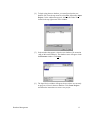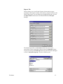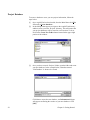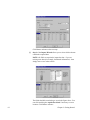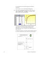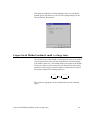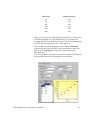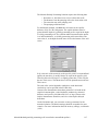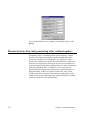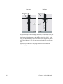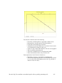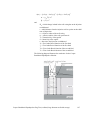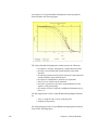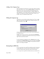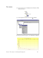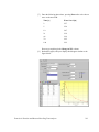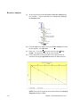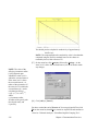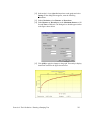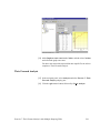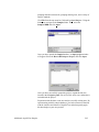
1
AquiferTest v.3.5 User’s Manual Advanced Pumping Test & Slug Test Analysis Software Images created using AquiferTest Pro 2002, Co-developed by Thomas Röhrich and Waterloo Hydrogeologic, Inc. December 2002 License Agreement Waterloo Hydrogeologic Inc. retains the ownership of this copy of the software. This copy is licensed to you for use under the following conditions: I. Copyright Notice This software is protected by both Canadian copyright law and international treaty provisions. Therefore, you must treat this software JUST LIKE A BOOK, with the following single exception. Waterloo Hydrogeologic Inc. authorizes you to make archive copies of the software for the sole purpose of backing-up our software and protecting your investment from loss. By saying "JUST LIKE A BOOK", Waterloo Hydrogeologic Inc. means, for example, that this software may be used by any number of people and may be freely moved from one computer location to another, so long as there is NO POSSIBILITY of it being used at one location while it is being used at another. Just like a book can't be read by two different people in two different places at the same time. Specifically, you may not distribute, rent, sub-license, or lease the software or documentation; alter, modify, or adapt the software or documentation, including, but not limited to, translating, decompiling, disassembling, or creating derivative works without the prior written consent of Waterloo Hydrogeologic Inc. The provided software and documentation contain trade secrets and it is agreed by the licensee that these trade secrets will not be disclosed to non-licensed persons without written consent of Waterloo Hydrogeologic Inc. II. Warranty Waterloo Hydrogeologic Inc. warrants that, under normal use, the material on the CD-ROM and the documentation will be free of defects in materials and workmanship for a period of 30 days from the date of purchase. In the event of notification of defects in material or workmanship, Waterloo Hydrogeologic Inc. will replace the CD-ROM or documentation. The remedy for breach of this warranty shall be limited to replacement and shall not encompass any other damages, including but not limited to loss of profit, and special, incidental, consequential, or other similar claims. III. Disclaimer Except as specifically provided above, neither the developer(s) of this software nor any person or organization acting on behalf of him (them) makes any warranty, express or implied, with respect to this software. In no event will Waterloo Hydrogeologic Inc. assume any liabilities with respect to the use, or misuse, of this software, or the interpretation, or misinterpretation, of any results obtained from this software, or for direct, indirect, special, incidental, or consequential damages resulting from the use of this software. Specifically, Waterloo Hydrogeologic Inc. is not responsible for any costs including, but not limited to, those incurred as a result of lost profits or revenue, loss of use of the computer program, loss of data, the costs of recovering such programs or data, the cost of any substitute program, claims by third parties, or for other similar costs. In no case shall Waterloo Hydrogeologic Inc.'s liability exceed the amount of the license fee. IV. Infringement Protection Waterloo Hydrogeologic Inc. is the sole owner of this software. Waterloo Hydrogeologic Inc. warrants that neither the software and documentation nor any component, including elements provided by others and incorporated into the software and documentation, infringes upon or violates any patent, trademark, copyright, trade secret, or other proprietary right. Royalties or other charges for any patent, trademark, copyright, trade secret or other proprietary information to be used in the software and documentation shall be considered as included in the contract price. V. Governing Law This license agreement shall be construed, interpreted, and governed by the laws of the Province of Ontario, Canada, and the United States. Any terms or conditions of this agreement found to be unenforceable, illegal, or contrary to public policy in any jurisdiction will be deleted, but will not affect the remaining terms and conditions of the agreement. VI. Entire Agreement This agreement constitutes the entire agreement between you and Waterloo Hydrogeologic, Inc. License Agreement December 2002 Table of Contents Preface i How to Contact Waterloo Hydrogeologic, Inc. . . . . . . . . . . . . . . . . . . . . . . . . . . . . . . . . . . . . . i Technical Support . . . . . . . . . . . . . . . . . . . . . . . . . . . . . . . . . . . . . . . . . . . . . . . . . . . . . . . . . . . i Waterloo Hydrogeologic, Inc. Training and Consulting . . . . . . . . . . . . . . . . . . . . . . . . . . . . . .ii Other Software Products by Waterloo Hydrogeologic, Inc. . . . . . . . . . . . . . . . . . . . . . . . . . . .ii Visual MODFLOW Pro . . . . . . . . . . . . . . . . . . . . . . . . . . . . . . . . . . . . . . . . . . . . . . . . . . .ii Visual MODFLOW 3D-Explorer. . . . . . . . . . . . . . . . . . . . . . . . . . . . . . . . . . . . . . . . . . . iii WinPEST . . . . . . . . . . . . . . . . . . . . . . . . . . . . . . . . . . . . . . . . . . . . . . . . . . . . . . . . . . . . . iii RISC WorkBench. . . . . . . . . . . . . . . . . . . . . . . . . . . . . . . . . . . . . . . . . . . . . . . . . . . . . . . iii Visual PEST . . . . . . . . . . . . . . . . . . . . . . . . . . . . . . . . . . . . . . . . . . . . . . . . . . . . . . . . . . . iii Visual Groundwater . . . . . . . . . . . . . . . . . . . . . . . . . . . . . . . . . . . . . . . . . . . . . . . . . . . . . iii WHI UnSat Suite . . . . . . . . . . . . . . . . . . . . . . . . . . . . . . . . . . . . . . . . . . . . . . . . . . . . . . . iii Visual HELP. . . . . . . . . . . . . . . . . . . . . . . . . . . . . . . . . . . . . . . . . . . . . . . . . . . . . . . . . . . iv MoNA ToolKit . . . . . . . . . . . . . . . . . . . . . . . . . . . . . . . . . . . . . . . . . . . . . . . . . . . . . . . . . iv AquaChem . . . . . . . . . . . . . . . . . . . . . . . . . . . . . . . . . . . . . . . . . . . . . . . . . . . . . . . . . . . . iv FLOWPATH II. . . . . . . . . . . . . . . . . . . . . . . . . . . . . . . . . . . . . . . . . . . . . . . . . . . . . . . . . iv 1. Introduction . . . . . . . . . . . . . . . . . . . . . . . . . . . . . . . . . . . . . . . . . . . . . . . . . . . . . . . 1 Database Concept . . . . . . . . . . . . . . . . . . . . . . . . . . . . . . . . . . . . . . . . . . . . . . . . . . . . . . . . . . . . 3 System Requirements . . . . . . . . . . . . . . . . . . . . . . . . . . . . . . . . . . . . . . . . . . . . . . . . . . . . . . . . .4 Installing AquiferTest . . . . . . . . . . . . . . . . . . . . . . . . . . . . . . . . . . . . . . . . . . . . . . . . . . . . . . . . 4 Online Help . . . . . . . . . . . . . . . . . . . . . . . . . . . . . . . . . . . . . . . . . . . . . . . . . . . . . . . . . . . . . . . . 5 Suggested Reference Material . . . . . . . . . . . . . . . . . . . . . . . . . . . . . . . . . . . . . . . . . . . . . . . . . . 5 2. Using AquiferTest . . . . . . . . . . . . . . . . . . . . . . . . . . . . . . . . . . . . . . . . . . . . . . . . . . 7 Window Layout . . . . . . . . . . . . . . . . . . . . . . . . . . . . . . . . . . . . . . . . . . . . . . . . . . . . . . . . . . . . .8 Navigator Tree . . . . . . . . . . . . . . . . . . . . . . . . . . . . . . . . . . . . . . . . . . . . . . . . . . . . . . . . . . 8 Properties Notebook . . . . . . . . . . . . . . . . . . . . . . . . . . . . . . . . . . . . . . . . . . . . . . . . . . . . . . 9 Database Management . . . . . . . . . . . . . . . . . . . . . . . . . . . . . . . . . . . . . . . . . . . . . . . . . . . . . . .11 Menu Bar and Icons . . . . . . . . . . . . . . . . . . . . . . . . . . . . . . . . . . . . . . . . . . . . . . . . . . . . . . . . . 16 File Menu . . . . . . . . . . . . . . . . . . . . . . . . . . . . . . . . . . . . . . . . . . . . . . . . . . . . . . . . . . . . . . . . .16 Create database . . . . . . . . . . . . . . . . . . . . . . . . . . . . . . . . . . . . . . . . . . . . . . . . . . . . . . . . . 16 New Project . . . . . . . . . . . . . . . . . . . . . . . . . . . . . . . . . . . . . . . . . . . . . . . . . . . . . . . . . . .16 Open Project . . . . . . . . . . . . . . . . . . . . . . . . . . . . . . . . . . . . . . . . . . . . . . . . . . . . . . . . . . . 16 Import . . . . . . . . . . . . . . . . . . . . . . . . . . . . . . . . . . . . . . . . . . . . . . . . . . . . . . . . . . . . . . . .16 Export . . . . . . . . . . . . . . . . . . . . . . . . . . . . . . . . . . . . . . . . . . . . . . . . . . . . . . . . . . . . . . . .21 Preferences... . . . . . . . . . . . . . . . . . . . . . . . . . . . . . . . . . . . . . . . . . . . . . . . . . . . . . . . . . . 22 Maps... . . . . . . . . . . . . . . . . . . . . . . . . . . . . . . . . . . . . . . . . . . . . . . . . . . . . . . . . . . . . . . . 26 Print Preview . . . . . . . . . . . . . . . . . . . . . . . . . . . . . . . . . . . . . . . . . . . . . . . . . . . . . . . . . . 26 Print . . . . . . . . . . . . . . . . . . . . . . . . . . . . . . . . . . . . . . . . . . . . . . . . . . . . . . . . . . . . . . . . . 26 Exit . . . . . . . . . . . . . . . . . . . . . . . . . . . . . . . . . . . . . . . . . . . . . . . . . . . . . . . . . . . . . . . . . .26 Edit Menu . . . . . . . . . . . . . . . . . . . . . . . . . . . . . . . . . . . . . . . . . . . . . . . . . . . . . . . . . . . . . . . . .26 Copy . . . . . . . . . . . . . . . . . . . . . . . . . . . . . . . . . . . . . . . . . . . . . . . . . . . . . . . . . . . . . . . . .26 Contents i Paste . . . . . . . . . . . . . . . . . . . . . . . . . . . . . . . . . . . . . . . . . . . . . . . . . . . . . . . . . . . . . . . . Delete . . . . . . . . . . . . . . . . . . . . . . . . . . . . . . . . . . . . . . . . . . . . . . . . . . . . . . . . . . . . . . . View Menu . . . . . . . . . . . . . . . . . . . . . . . . . . . . . . . . . . . . . . . . . . . . . . . . . . . . . . . . . . . . . . . Results. . . . . . . . . . . . . . . . . . . . . . . . . . . . . . . . . . . . . . . . . . . . . . . . . . . . . . . . . . . . . . . Symbol List. . . . . . . . . . . . . . . . . . . . . . . . . . . . . . . . . . . . . . . . . . . . . . . . . . . . . . . . . . . Small Tool Buttons . . . . . . . . . . . . . . . . . . . . . . . . . . . . . . . . . . . . . . . . . . . . . . . . . . . . . Units Converter. . . . . . . . . . . . . . . . . . . . . . . . . . . . . . . . . . . . . . . . . . . . . . . . . . . . . . . . Enlarge Graph . . . . . . . . . . . . . . . . . . . . . . . . . . . . . . . . . . . . . . . . . . . . . . . . . . . . . . . . . Project Menu. . . . . . . . . . . . . . . . . . . . . . . . . . . . . . . . . . . . . . . . . . . . . . . . . . . . . . . . . . . . . . Create Well... . . . . . . . . . . . . . . . . . . . . . . . . . . . . . . . . . . . . . . . . . . . . . . . . . . . . . . . . . Map... . . . . . . . . . . . . . . . . . . . . . . . . . . . . . . . . . . . . . . . . . . . . . . . . . . . . . . . . . . . . . . . Units . . . . . . . . . . . . . . . . . . . . . . . . . . . . . . . . . . . . . . . . . . . . . . . . . . . . . . . . . . . . . . . . Test Menu . . . . . . . . . . . . . . . . . . . . . . . . . . . . . . . . . . . . . . . . . . . . . . . . . . . . . . . . . . . . . . . . Create pumping test . . . . . . . . . . . . . . . . . . . . . . . . . . . . . . . . . . . . . . . . . . . . . . . . . . . . Create slug test . . . . . . . . . . . . . . . . . . . . . . . . . . . . . . . . . . . . . . . . . . . . . . . . . . . . . . . . Units . . . . . . . . . . . . . . . . . . . . . . . . . . . . . . . . . . . . . . . . . . . . . . . . . . . . . . . . . . . . . . . . Data Menu . . . . . . . . . . . . . . . . . . . . . . . . . . . . . . . . . . . . . . . . . . . . . . . . . . . . . . . . . . . . . . . New . . . . . . . . . . . . . . . . . . . . . . . . . . . . . . . . . . . . . . . . . . . . . . . . . . . . . . . . . . . . . . . . . Import . . . . . . . . . . . . . . . . . . . . . . . . . . . . . . . . . . . . . . . . . . . . . . . . . . . . . . . . . . . . . . . Data Logger File . . . . . . . . . . . . . . . . . . . . . . . . . . . . . . . . . . . . . . . . . . . . . . . . . . . . . . . Analysis Menu . . . . . . . . . . . . . . . . . . . . . . . . . . . . . . . . . . . . . . . . . . . . . . . . . . . . . . . . . . . . Create . . . . . . . . . . . . . . . . . . . . . . . . . . . . . . . . . . . . . . . . . . . . . . . . . . . . . . . . . . . . . . . Data... . . . . . . . . . . . . . . . . . . . . . . . . . . . . . . . . . . . . . . . . . . . . . . . . . . . . . . . . . . . . . . . Settings.... . . . . . . . . . . . . . . . . . . . . . . . . . . . . . . . . . . . . . . . . . . . . . . . . . . . . . . . . . . . . Properties... . . . . . . . . . . . . . . . . . . . . . . . . . . . . . . . . . . . . . . . . . . . . . . . . . . . . . . . . . . . Method . . . . . . . . . . . . . . . . . . . . . . . . . . . . . . . . . . . . . . . . . . . . . . . . . . . . . . . . . . . . . . Analysis state . . . . . . . . . . . . . . . . . . . . . . . . . . . . . . . . . . . . . . . . . . . . . . . . . . . . . . . . . Help Menu . . . . . . . . . . . . . . . . . . . . . . . . . . . . . . . . . . . . . . . . . . . . . . . . . . . . . . . . . . . . . . . Contents... . . . . . . . . . . . . . . . . . . . . . . . . . . . . . . . . . . . . . . . . . . . . . . . . . . . . . . . . . . . . About... . . . . . . . . . . . . . . . . . . . . . . . . . . . . . . . . . . . . . . . . . . . . . . . . . . . . . . . . . . . . . . 26 27 27 27 27 27 28 28 28 28 29 31 31 31 32 33 34 34 35 36 43 43 43 44 44 46 46 47 47 47 3. Getting Started. . . . . . . . . . . . . . . . . . . . . . . . . . . . . . . . . . . . . . . . . . . . . . . . . . . . 49 Creating a New Project. . . . . . . . . . . . . . . . . . . . . . . . . . . . . . . . . . . . . . . . . . . . . . . . . . . . . . Project Database . . . . . . . . . . . . . . . . . . . . . . . . . . . . . . . . . . . . . . . . . . . . . . . . . . . . . . . Project Units . . . . . . . . . . . . . . . . . . . . . . . . . . . . . . . . . . . . . . . . . . . . . . . . . . . . . . . . . . Project Maps . . . . . . . . . . . . . . . . . . . . . . . . . . . . . . . . . . . . . . . . . . . . . . . . . . . . . . . . . . Well Locations and Geometry . . . . . . . . . . . . . . . . . . . . . . . . . . . . . . . . . . . . . . . . . . . . Creating a Pumping Test . . . . . . . . . . . . . . . . . . . . . . . . . . . . . . . . . . . . . . . . . . . . . . . . . . . . Pumping Test Units . . . . . . . . . . . . . . . . . . . . . . . . . . . . . . . . . . . . . . . . . . . . . . . . . . . . Creating a Pumping Test Analysis . . . . . . . . . . . . . . . . . . . . . . . . . . . . . . . . . . . . . . . . . Creating a Slug Test . . . . . . . . . . . . . . . . . . . . . . . . . . . . . . . . . . . . . . . . . . . . . . . . . . . . . . . . Slug Test Units . . . . . . . . . . . . . . . . . . . . . . . . . . . . . . . . . . . . . . . . . . . . . . . . . . . . . . . . Importing Observation Well Water Level Data from a Text File. . . . . . . . . . . . . . . . . . Creating a Slug Test Analysis. . . . . . . . . . . . . . . . . . . . . . . . . . . . . . . . . . . . . . . . . . . . . 49 50 53 54 59 64 65 75 77 78 79 83 4. Analysis Methods . . . . . . . . . . . . . . . . . . . . . . . . . . . . . . . . . . . . . . . . . . . . . . . . . . 87 ii Contents Definition of Symbols . . . . . . . . . . . . . . . . . . . . . . . . . . . . . . . . . . . . . . . . . . . . . . . . . . . . . . . 87 Pumping Tests and Slug Tests . . . . . . . . . . . . . . . . . . . . . . . . . . . . . . . . . . . . . . . . . . . . . . . . . 90 Automatic Curve Fitting. . . . . . . . . . . . . . . . . . . . . . . . . . . . . . . . . . . . . . . . . . . . . . . . . . 91 Manual Curve Fitting . . . . . . . . . . . . . . . . . . . . . . . . . . . . . . . . . . . . . . . . . . . . . . . . . . . . 91 Radial Flow to a Well in a Confined Aquifer . . . . . . . . . . . . . . . . . . . . . . . . . . . . . . . . . . . . . 92 Drawdown vs. Time . . . . . . . . . . . . . . . . . . . . . . . . . . . . . . . . . . . . . . . . . . . . . . . . . . . . . 93 Drawdown vs. Time with Discharge . . . . . . . . . . . . . . . . . . . . . . . . . . . . . . . . . . . . . . . . 94 Solution Method Advisor . . . . . . . . . . . . . . . . . . . . . . . . . . . . . . . . . . . . . . . . . . . . . . . . . . . . . 94 Pumping Test Analyses . . . . . . . . . . . . . . . . . . . . . . . . . . . . . . . . . . . . . . . . . . . . . . . . . . . . . . 96 Theis Method (confined) . . . . . . . . . . . . . . . . . . . . . . . . . . . . . . . . . . . . . . . . . . . . . . . . . . . . . 96 Cooper-Jacob Method (confined; small r or large time) . . . . . . . . . . . . . . . . . . . . . . . . . . . . . 99 Cooper-Jacob Time-Drawdown Method . . . . . . . . . . . . . . . . . . . . . . . . . . . . . . . . . . . . 100 Cooper-Jacob Distance-Drawdown Method . . . . . . . . . . . . . . . . . . . . . . . . . . . . . . . . . 102 Cooper-Jacob Time-Distance-Drawdown Method. . . . . . . . . . . . . . . . . . . . . . . . . . . . . 103 Theis Recovery Test (confined) . . . . . . . . . . . . . . . . . . . . . . . . . . . . . . . . . . . . . . . . . . . . . . . 105 Neuman Method (unconfined) . . . . . . . . . . . . . . . . . . . . . . . . . . . . . . . . . . . . . . . . . . . . . . . . 108 Hantush-Jacob (Walton) Method (leaky, no aquitard storage) . . . . . . . . . . . . . . . . . . . . . . .111 Specific Capacity . . . . . . . . . . . . . . . . . . . . . . . . . . . . . . . . . . . . . . . . . . . . . . . . . . . . . . . . . .114 Cooper-Jacob Steptest (variable discharge rate) . . . . . . . . . . . . . . . . . . . . . . . . . . . . . . . . . . 116 Theis Steptest (Birsoy and Summers, confined) . . . . . . . . . . . . . . . . . . . . . . . . . . . . . . . . . . 119 Jacob Correction for Unconfined Conditions. . . . . . . . . . . . . . . . . . . . . . . . . . . . . . . . . . . . .124 Moench Method (partially penetrating well in confined or unconfined aquifers) . . . . . . . . .124 Moench (fracture flow, fully penetrating wells, confined aquifer) . . . . . . . . . . . . . . . . . . . . 128 Hantush-Bierschenk Well Loss Solution . . . . . . . . . . . . . . . . . . . . . . . . . . . . . . . . . . . . . . . . 134 Theis Prediction (Pumping Test Planning) Solution . . . . . . . . . . . . . . . . . . . . . . . . . . . . . . .140 Forward Solutions . . . . . . . . . . . . . . . . . . . . . . . . . . . . . . . . . . . . . . . . . . . . . . . . . . . . . . . . . 143 Theory of Superposition. . . . . . . . . . . . . . . . . . . . . . . . . . . . . . . . . . . . . . . . . . . . . . . . . . . . . 143 Background Information on the Forward Solutions Algorithm . . . . . . . . . . . . . . . . . . . . . . . 143 Influence of Multiple Pumping Wells . . . . . . . . . . . . . . . . . . . . . . . . . . . . . . . . . . . . . . 144 Step Drawdown and Recovery Test (Variable Discharge Rates). . . . . . . . . . . . . . . . . .145 Partially Penetrating Wells . . . . . . . . . . . . . . . . . . . . . . . . . . . . . . . . . . . . . . . . . . . . . . . 148 Measuring Drawdown in the Well . . . . . . . . . . . . . . . . . . . . . . . . . . . . . . . . . . . . . . . . . 151 Inversion Algorithm . . . . . . . . . . . . . . . . . . . . . . . . . . . . . . . . . . . . . . . . . . . . . . . . . . . . 151 Iteration Paths. . . . . . . . . . . . . . . . . . . . . . . . . . . . . . . . . . . . . . . . . . . . . . . . . . . . . . . . . 158 Forward Solution Functionality . . . . . . . . . . . . . . . . . . . . . . . . . . . . . . . . . . . . . . . . . . . 158 Theis Forward Solution . . . . . . . . . . . . . . . . . . . . . . . . . . . . . . . . . . . . . . . . . . . . . . . . . . . . . 161 Hantush-Jacob Forward Solution . . . . . . . . . . . . . . . . . . . . . . . . . . . . . . . . . . . . . . . . . . . . . .162 Stallman Forward Solution (Barrier and Recharge Boundaries) . . . . . . . . . . . . . . . . . . . . . . 164 Gringarten-Bourdet Forward Solution (Well Skin Effects) . . . . . . . . . . . . . . . . . . . . . . . . . . 170 Papadopulos Forward Solution (Large Diameter Wells) . . . . . . . . . . . . . . . . . . . . . . . . . . . .173 Slug Test Analyses . . . . . . . . . . . . . . . . . . . . . . . . . . . . . . . . . . . . . . . . . . . . . . . . . . . . . . . . . 177 Bouwer-Rice Slug Test (unconfined or leaky confined, fully or partially penetrating well).177 Hvorslev Slug Test (confined or unconfined aquifer, fully or partially penetrating well). . . 181 Cooper-Bredehoeft-Papadopulos Slug Test (confined, large diameter well with storage) . . 186 References . . . . . . . . . . . . . . . . . . . . . . . . . . . . . . . . . . . . . . . . . . . . . . . . . . . . . . . . . . . . . . . 189 Contents iii 5. Producing Reports . . . . . . . . . . . . . . . . . . . . . . . . . . . . . . . . . . . . . . . . . . . . . . . . 193 Report Editor . . . . . . . . . . . . . . . . . . . . . . . . . . . . . . . . . . . . . . . . . . . . . . . . . . . . . . . . . . . . Report Editor Layout . . . . . . . . . . . . . . . . . . . . . . . . . . . . . . . . . . . . . . . . . . . . . . . . . . Static elements . . . . . . . . . . . . . . . . . . . . . . . . . . . . . . . . . . . . . . . . . . . . . . . . . . . . . . . Adding a New Static Element. . . . . . . . . . . . . . . . . . . . . . . . . . . . . . . . . . . . . . . . . . . . Dynamic elements. . . . . . . . . . . . . . . . . . . . . . . . . . . . . . . . . . . . . . . . . . . . . . . . . . . . . Adding a New Company Logo . . . . . . . . . . . . . . . . . . . . . . . . . . . . . . . . . . . . . . . . . . . Editing the Company Logo. . . . . . . . . . . . . . . . . . . . . . . . . . . . . . . . . . . . . . . . . . . . . . Backup Report (.REP) Files . . . . . . . . . . . . . . . . . . . . . . . . . . . . . . . . . . . . . . . . . . . . . 193 193 194 196 196 197 197 197 6. Demonstration Exercises . . . . . . . . . . . . . . . . . . . . . . . . . . . . . . . . . . . . . . . . . . . 199 Exercise 1: Theis Analysis - Confined Aquifer Pumping Test. . . . . . . . . . . . . . . . . . . . . . . New Project. . . . . . . . . . . . . . . . . . . . . . . . . . . . . . . . . . . . . . . . . . . . . . . . . . . . . . . . . . Wells . . . . . . . . . . . . . . . . . . . . . . . . . . . . . . . . . . . . . . . . . . . . . . . . . . . . . . . . . . . . . . . Pumping Test . . . . . . . . . . . . . . . . . . . . . . . . . . . . . . . . . . . . . . . . . . . . . . . . . . . . . . . . Observed Data. . . . . . . . . . . . . . . . . . . . . . . . . . . . . . . . . . . . . . . . . . . . . . . . . . . . . . . . Theis Analysis. . . . . . . . . . . . . . . . . . . . . . . . . . . . . . . . . . . . . . . . . . . . . . . . . . . . . . . . Zooming In and Out . . . . . . . . . . . . . . . . . . . . . . . . . . . . . . . . . . . . . . . . . . . . . . . . . . . Moving the Curve . . . . . . . . . . . . . . . . . . . . . . . . . . . . . . . . . . . . . . . . . . . . . . . . . . . . . Printing . . . . . . . . . . . . . . . . . . . . . . . . . . . . . . . . . . . . . . . . . . . . . . . . . . . . . . . . . . . . . Exercise 2: Cooper-Jacob Analysis Confined Aquifer Pumping Test . . . . . . . . . . . . . . . . . Cooper-Jacob Analysis . . . . . . . . . . . . . . . . . . . . . . . . . . . . . . . . . . . . . . . . . . . . . . . . . Removing Unwanted Data Points. . . . . . . . . . . . . . . . . . . . . . . . . . . . . . . . . . . . . . . . . Correction for Unconfined Conditions . . . . . . . . . . . . . . . . . . . . . . . . . . . . . . . . . . . . . Exercise 3: Theis Recovery Analysis with Data Logger Data . . . . . . . . . . . . . . . . . . . . . . . Observation Well . . . . . . . . . . . . . . . . . . . . . . . . . . . . . . . . . . . . . . . . . . . . . . . . . . . . . Observed Data. . . . . . . . . . . . . . . . . . . . . . . . . . . . . . . . . . . . . . . . . . . . . . . . . . . . . . . . Data Logger File . . . . . . . . . . . . . . . . . . . . . . . . . . . . . . . . . . . . . . . . . . . . . . . . . . . . . . Recovery Analysis . . . . . . . . . . . . . . . . . . . . . . . . . . . . . . . . . . . . . . . . . . . . . . . . . . . . Exercise 4: Hvorslev and Bouwer-Rice Slug Test Analyses . . . . . . . . . . . . . . . . . . . . . . . . Observation Well . . . . . . . . . . . . . . . . . . . . . . . . . . . . . . . . . . . . . . . . . . . . . . . . . . . . . Slug Test . . . . . . . . . . . . . . . . . . . . . . . . . . . . . . . . . . . . . . . . . . . . . . . . . . . . . . . . . . . . Hvorslev Analysis. . . . . . . . . . . . . . . . . . . . . . . . . . . . . . . . . . . . . . . . . . . . . . . . . . . . . Bouwer-Rice Analysis . . . . . . . . . . . . . . . . . . . . . . . . . . . . . . . . . . . . . . . . . . . . . . . . . Exercise 5: Moench Analysis - Unconfined Aquifer Pumping Test . . . . . . . . . . . . . . . . . . New Project. . . . . . . . . . . . . . . . . . . . . . . . . . . . . . . . . . . . . . . . . . . . . . . . . . . . . . . . . . Wells . . . . . . . . . . . . . . . . . . . . . . . . . . . . . . . . . . . . . . . . . . . . . . . . . . . . . . . . . . . . . . . Pumping Test . . . . . . . . . . . . . . . . . . . . . . . . . . . . . . . . . . . . . . . . . . . . . . . . . . . . . . . . Observed Data. . . . . . . . . . . . . . . . . . . . . . . . . . . . . . . . . . . . . . . . . . . . . . . . . . . . . . . . Moench Analysis . . . . . . . . . . . . . . . . . . . . . . . . . . . . . . . . . . . . . . . . . . . . . . . . . . . . . Exercise 6: Theis Prediction - Planning a Pumping Test . . . . . . . . . . . . . . . . . . . . . . . . . . . Exercise 7: Theis Forward Analysis with Multiple Pumping Wells . . . . . . . . . . . . . . . . . . Wells . . . . . . . . . . . . . . . . . . . . . . . . . . . . . . . . . . . . . . . . . . . . . . . . . . . . . . . . . . . . . . . Pumping Test . . . . . . . . . . . . . . . . . . . . . . . . . . . . . . . . . . . . . . . . . . . . . . . . . . . . . . . . Observed Data. . . . . . . . . . . . . . . . . . . . . . . . . . . . . . . . . . . . . . . . . . . . . . . . . . . . . . . . Theis Forward Analysis . . . . . . . . . . . . . . . . . . . . . . . . . . . . . . . . . . . . . . . . . . . . . . . . iv 200 200 202 203 204 209 212 213 214 216 216 217 221 223 223 223 225 229 232 232 232 234 235 237 237 238 240 240 244 249 254 255 256 259 261 Contents Additional AquiferTest Samples . . . . . . . . . . . . . . . . . . . . . . . . . . . . . . . . . . . . . . . . . . . . . . 264 Contents v vi Contents Preface How to Contact Waterloo Hydrogeologic, Inc. If after reading this manual and using AquiferTest you would like to contact Waterloo Hydrogeologic with comments or suggestions, or if you need technical assistance, you can reach us at: Waterloo Hydrogeologic Inc. 460 Phillip Street - Suite 101 Waterloo, Ontario, CANADA N2L 5J2 Phone +1 (519) 746 1798 Fax +1 (519) 885 5262 E-mail: [email protected] Web: www.waterloohydrogeologic.com Technical Support To help us handle your technical support questions as quickly as possible, please have the following information ready before you call, or include it in a detailed technical support e-mail: • A complete description of the problem including a summary of key strokes and program events • Product name and version number • Product serial number • Computer make and model number • Operating system and version number • Total free RAM • Number of free bytes on your hard disk You may send us your questions via e-mail, fax, or call one of our technical support specialists. Please allow up to two business days for a response. How to Contact Waterloo Hydrogeologic, Inc. i Waterloo Hydrogeologic, Inc. Training and Consulting Waterloo Hydrogeologic strives to offer the most useful, practical, high quality training in hydrogeologic modeling in the industry. Training courses are designed to provide a rapid introduction to essential knowledge and skills, and create a basis for further professional development and real-world practice. Open enrollment courses are offered worldwide each year. For the current schedule of courses, visit: www.waterloohydrogeologic.com or e-mail us at: [email protected]. Waterloo Hydrogeologic also offers expert consulting and reviewing services for all numerical modeling projects concerning groundwater flow and solute transport. For further information, please contact us at: [email protected]. Other Software Products by Waterloo Hydrogeologic, Inc. We also develop and distribute a number of other useful software products for the groundwater professional, all designed to increase your efficiency and enhance your technical capability, including: • • • • • • • • • • • Visual MODFLOW Pro Visual MODFLOW 3D-Explorer WinPEST RISC WorkBench Visual PEST Visual Groundwater WHI UnSatSuite Visual HELP MoNA ToolKit AquaChem FLOWPATH II Visual MODFLOW Pro ...is the largest time-saving breakthrough since the release of MODFLOW for building, calibrating, and analyzing groundwater flow and contaminant transport models. Setting the environmental industry standard, Visual MODFLOW Pro is a pre- and post-processor for MODFLOW, MODPATH, and MT3D/RT3D. Visual MODFLOW Pro is the complete package for groundwater modeling and includes the Visual MODFLOW 3D-Explorer and WinPEST (see descriptions below). ii Visual MODFLOW 3D-Explorer ...is a built-in 3D visualization system for displaying and animating Visual MODFLOW models using state-of-the-art 3D graphics technology. The advanced visualization capabilities of the Visual MODFLOW 3D-Explorer provide you with all the tools you need to create impressive and informative 3D representations of your modeling data using vibrant colors and high-resolution graphics. WinPEST ...is exclusively designed for Visual MODFLOW Pro to help reduce the tedious hours spent calibrating model results to observations found in the field. WinPEST is completely integrated within Visual MODFLOW Pro and offers a variety of benefits unparalleled in other calibration packages. RISC WorkBench ...is an easy-to-use software package designed for performing fate and transport modeling and human health risk assessments for contaminated sites. Following standard procedures outlined by the U.S. EPA, the RISC WorkBench calculates exposure assessment, toxicity assessment, and risk assessment. RISC WorkBench also includes a completely customizable database for common environmental parameters used when conducting risk assessments. Visual PEST ...combines the latest version of PEST2000 with the graphical processing and display features of WinPEST for model-independent parameter estimation. Visual Groundwater ...is the first software package to combine state-of-the-art graphical technology for 3D visualization and animation capabilities with an easyto-use graphical interface designed specifically for environmental project applications. WHI UnSat Suite ...is a fully-integrated software package for modeling 1D unsaturated zone flow and contaminant transport using the industry standard numerical modeling codes - all run under one tightly integrated interface. Other Software Products by Waterloo Hydrogeologic, Inc. iii Visual HELP ...is the most advanced hydrological modeling environment available for designing landfills, predicting leachate mounding and evaluating potential leachate seepage to the groundwater table. MoNA ToolKit ...provides an integrated data management, visualization, trend analysis, and modeling platform for evaluating the effectiveness of Monitored Natural Attenuation. The MoNA ToolKit combines 3 different software applications (BioTrends, SEQUENCE and BioTracker) into one integrated solution for evaluating, visualizing and modeling natural attenuation processes. AquaChem ...is a fully integrated software package developed specifically for numerical analysis of aqueous geochemical data. These powerful analytical capabilities are complimented by a comprehensive selection of commonly used graphical techniques to portray the chemical characteristics of geochemical and water quality data for single samples and groups of samples. AquaChem is truly one of the most powerful tools available for dealing with the interpretation, analysis and modeling of simple or complex geochemical data sets. FLOWPATH II ...is a popular two-dimensional, steady-state, groundwater flow, pathline, and contaminant transport model that computes hydraulic heads, pathlines, travel times, velocities, water balances, and contaminant concentrations (approved by the US EPA and recommended by the UK Environmental Agency). At Waterloo Hydrogeologic, we are continually developing new modeling and visualization applications for the environmental professional. For more information, please contact us. iv 1 Introduction Congratulations on your purchase of AquiferTest, the most popular software package available for graphical analysis and reporting of pumping test and slug test data! AquiferTest is designed by hydrogeologists for hydrogeologists giving you all the tools you need to efficiently manage hydraulic testing results and provide a selection of the most commonly used solution methods for data analysis - all in the familiar and easy-to-use Microsoft Windows environment. AquiferTest 3.5 has the following key features and enhancements: • Runs as a native Windows 98/NT/2000/XP 32-bit application • Easy-to-use, intuitive interface • Solution methods for unconfined, confined, leaky confined and fractured rock aquifers • Customizable report templates, with a built-in report designer • Solution Method Advisor (see page 94) to assist you in choosing an appropriate data analysis method • Easily create and compare multiple analysis methods for the same data set • Step test/well loss method • Pumping test planning “forward solution” methods • Single well solutions • Universal Data Logger Import utility (supports a wide variety of column delimiters and file layouts) • Import well locations and geometry from an ASCII file • Site map support for .dxf files and bitmap (.bmp) images • Windows clipboard support for cutting and pasting of data and output graphics directly into your project report • Export analysis graphs to a graphics file (.bmp, .jpg, .wmf, .emf) • Dockable, customizable tool bar • Numerous short-cut keys to speed program navigation • Units converter • Microsoft Access database-driven application for enhanced usability and efficiency • Unlimited free technical support from WHI 1 For pumping tests, the following solution methods are available: • • • • • • • • • • • • • • Theis (1935) Cooper-Jacob Time-Drawdown (1946) Cooper-Jacob Distance-Drawdown (1946) Cooper-Jacob Time-Distance-Drawdown (1946) Hantush-Jacob (1955) Neuman (1975) Moench (1993) Moench Fracture Flow (1984) Theis Steptest (1935) Cooper-Jacob Steptest (1946) Theis Recovery (1935) Hantush-Bierschenk Well Loss (1964) Specific Capacity Test Theis Prediction (pumping test planning) For slug tests, the following solution methods are available: • Hvorslev (1951) • Bouwer-Rice (1976) • Cooper-Bredehoeft-Papadopulos (1967) In addition, the following forward / predictive solutions for pumping tests are available in AquiferTest Pro: • • • • • • Theis (1937) Hantush (1955) Stallman-Barrier (1963) Stallman-Recharge (1963) Gringarten (1979) Papadopulos (1967) For more information on AquiferTest Pro or to order an upgrade, please contact us directly (Tel: 519-746-1798, Fax: 519-885-5262, Email: [email protected]). Data can be imported directly from: • Microsoft Excel version 4.0, 5.0, or 7.0 files • Data logger ASCII files with a variety of delimiters and column layouts AquiferTest provides a flexible, user-friendly environment that will allow you to become more efficient in your aquifer testing projects. Data can be directly entered in AquiferTest via the keyboard, imported from a Microsoft Excel (version 4, 5, or 7) workbook file, or imported from any data logger file (in ASCII format). Test data can also be inserted from a Windows text editor, spreadsheet, or database by “cutting and pasting” through the clipboard. 2 Introduction Automatic type curve fitting to a data set using least squares regression can be performed for standard graphical solution methods in AquiferTest (see page 91). However, you are encouraged to use your professional judgement to validate the graphical match based on your knowledge of the geologic and hydrogeologic setting of the test. To easily refine the curve fit, you can manually fit the data to a type curve by simply pressing the arrow keys on your keyboard (see page 91). NOTE: AquiferTest Pro forward solutions are solved using a non-linear inverse algorithm. For more information, please see Chapter 4: Forward Solutions on page 143. The demonstration exercises in Chapter 6 on page 199 will introduce you to many features of AquiferTest. The first two exercises evaluate pumping tests in a confined aquifer using the Theis and Cooper-Jacob methods. The third exercise uses the import capabilities of AquiferTest to import water level recovery data from a data logger, and subsequently analyzes it using the Theis Recovery method. The fourth exercise involves the evaluation of a slug test using both the Hvorslev and Bouwer-Rice methods. The fifth exercise uses the Moench method, while the sixth uses the Theis Prediction (forward) solution to answer commonly encountered questions when planning a pumping test. Finally, Exercise 7 examines a multiple pumping well analysis using an advanced forward / predictive solution method (available in AquiferTest Pro). Database Concept A program using a database has many advantages such as inherent data consistency and integrity, and inter operability (other database programs can access the data in the database). This can be important if you want to share your project data with others on a local area network (intranet) or with project colleagues on another continent via the Internet. AquiferTest stores its data in a database. Immediately after you enter or make changes to your data, the data are saved to the project database. For example, if you modify the project name, the change is saved to the database as soon as you leave the project name field. It is for this reason that there is no Save or Save as menu items in the program. Database Concept 3 System Requirements To run AquiferTest you need the following minimum system configuration: • • • • • A CD-ROM drive for software installation A hard drive, with at least 35 MB free A local or network printer installed A Pentium processor or better, with 32 MB Ram Windows 95/98/2000, or Windows NT 4.0 with Service Pack 3 (or later) installed • A Microsoft mouse or compatible • Minimum 600 x 800 screen resolution • Recommended 1024 x 768 screen resolution Installing AquiferTest AquiferTest is distributed on one CD-ROM. Place the CD into your CD-ROM drive and the initial installation screen should load automatically. Once loaded, an installation interface with several different tabs will be presented. Please take the time to explore the installation interface, as there is information concerning other Waterloo Hydrogeologic products, our worldwide distributors, technical support, consulting, training, and how to contact us. On the initial Installation tab, you may choose from the following two buttons: • AquiferTest 3.5 User’s Manual • AquiferTest 3.5 Installation The User’s Manual button will display a PDF document of the manual, which requires the Adobe Reader to view. If you do not have the Adobe Reader, a link has been created in the interface to download the appropriate software. The Installation button will initiate the installation of the software on your computer. AquiferTest must be installed on your hard disk in order to run. Please follow the installation instructions, and read the on-screen directions carefully. Once the installation is completed, you must re-boot your computer for the system changes to take effect. After the installation is complete and your system has re-booted, you should see the blue WHI icon on your Desktop screen labeled AquiferTest 3.5. To start working with AquiferTest, double-click this icon. 4 Introduction NOTE: To install the software from the CD-ROM without the aid of the installation interface, you can: • Open Windows Explorer, and navigate to the CD-ROM drive • Open the Installation folder • Double-click on the Setup32.exe to initiate the installation Follow the on-screen installation instructions, which will lead you through the install and subsequently produce a desktop icon for you. Online Help This book is supplied to you in two forms: as a printed book, and as an online help file. To view the online help version of this manual, select Help, then Contents. Suggested Reference Material Additional information can be obtained from hydrogeology texts such as Freeze and Cherry (1979), Kruseman and de Ridder (1979, 1990), Driscol (1987), Fetter (1988), Dominico and Schwartz (1990), and Walton (1996). In addition, several key publications are cited at the end of Chapter 4 (see page 189). Online Help 5 6 Introduction 2 Using AquiferTest AquiferTest is designed to automate the most common tasks that hydrogeologists and other water supply professionals typically encounter when planning and analyzing the results of an aquifer test. The program design allows you to efficiently manage all information from your aquifer test and perform more analyses in less time. For example, you need to enter information about your testing wells (e.g. X and Y coordinates, elevation, screen length, etc.) only once in AquiferTest. Each well and related information is stored in the project database separately from imported data and test analyses. After you create a well, you can see it in a navigator (project tree) view. When you import data or create an analysis, you specify which wells to include from the list of available wells in the project. If you decide to perform additional analyses, you can again specify from the available wells without re-creating them in AquiferTest. You can also change your solution method interactively while in analysis view by simply right-clicking the mouse and selecting one of the methods supplied with AquiferTest. There is no need to re-enter your data or create a new project. Your analysis graph is refreshed, and the data re-analyzed using the selected solution method. This is useful for quickly comparing the results of data analysis using slightly different solution methods. If you need solution-specific information for the re-analysis, AquiferTest prompts you for the required data. In the following sections, the features available in AquiferTest are described in detail. 7 Window Layout A typical AquiferTest window is shown above. The different sections of the window are described below. Navigator Tree The navigator section shows the wells, tests, and analyses for the current project in a standard tree view. As with other Windows applications, you can use the + or - icon to expand or collapse an element in the tree. Creating and deleting elements contained within the tree, including wells, data lists, pumping tests, slug tests, and associated analyses is discussed later in this chapter. 8 Chapter 2: Using AquiferTest Properties Notebook In AquiferTest, the data you enter is displayed in a standard Windows properties notebook. You can freely move from one page to another by using the tabs at the top of each page. A variety of different pages, or tabs, are encountered when using AquiferTest, including: • • • • • • • Project tab - contains project description and map Well tab - contains selected well location and dimensions Data tab - contains data for selected well Pumping test tab - contains pumping test details Slug test tab - contains slug test details Analysis tab - contains selected analysis and associated options Summary tab - contains a summary of analyses for selected test The available tabs in the Properties Notebook vary depending on which well, data list, or test is highlighted in the Navigator tree. For example, when conducting a pumping test there are three available tabs: • Project • Pumping test • Analysis Window Layout 9 In the Analysis notebook page for both the Pumping and Slug tests, there are two options for choosing the analysis method. By clicking on the pull-down arrow beside the Analysis Method, you have the option to change the CURRENT analysis type, as shown in the figure below: Conversely, by pressing the Create Analysis icon you can create a NEW analysis of your choice for the current data set. If you select this option, the test will be displayed and added to the navigator tree automatically 10 Chapter 2: Using AquiferTest Database Management AquiferTest saves all of its input and analysis data in a database file. In the following section, several basic database management techniques are described in detail. Mastering these activities will make managing your data easier and increase the speed of the program. Import and export of data for individual pumping tests AquiferTest allows the user to import and export individual pumping tests or entire projects. If you want to transfer an individual pumping test to another user of AquiferTest, you certainly do not want to have to transfer your entire database, since your database contains all of the data for all of your projects. To create a file for transferring either data from an entire project or from a single test, [1] Open the appropriate project with File/Open. [2] Highlight the Project or Test that you want to transfer in the Tree Navigator. [3] Select File/Export and then Project or Test as appropriate. [4] Input a file name and click [OK]. AquiferTest will then create a transfer file with the extension .AEX. Database Management 11 Now, to import this file select File/Import and then Project or Test, depending on whether you want to import the tests in the file as a new project or if you want to add the tests to the current open project. Creating a new database If you have a large number of pumping tests to input and analyze, your database will become very large which can lead to slow access time for the project. Therefore, it may be useful to split up your data into multiple databases if you have a large number of pumping tests. To create a new database: 12 [1] From the main menu, select File, followed by Create database... [2] In the Save as dialogue window that appears, type the name of the database you want to create. [3] Click [Save] to create the database. You will be prompted with a message indicating that the database has been created. Click [OK]. Chapter 2: Using AquiferTest Database Management [4] To begin using the new database, you must first select the new database file. From the top menu bar, select File, followed by Open Project... In the window that appears, click on the Folder icon located in the top-right corner of the window. [5] In the window that appears, select the new database (file extension .mdb, or Microsoft Database). The database name will appear in the the File name window. Click Open. [6] The Open Project window will appear, however there are currently no projects to select in the new database. Click Create Project... and follow the instructions to create a new project. 13 [7] The new project will appear in the Open Project window. Select the project (becomes highlighted) and click Open. You have completed the steps required to create a new database. Now, you may create as many projects as required within your new database. 14 Chapter 2: Using AquiferTest Deleting an Object To delete a well, pumping test, slug test, data object, or analysis object: [1] Select the object in the navigator view by left-clicking to highlight it. [2] Press the Delete key. [3] When prompted for confirmation, select YES. Be certain that you want to delete the object. There is no undo function. Deleting an Existing Project To delete an existing project: Database Management [1] Click File from the top menu bar, followed by Open Project. [2] Highlight the project you would like to permanently delete, and then click Delete... [3] When prompted for confirmation, click YES. 15 Menu Bar and Icons The following sections describe each of the items on the menu bar, and the equivalent icons. For a short description of an icon, move the mouse pointer over the icon without clicking either mouse button. File Menu The File menu contains the following items: Create database Create a new AquiferTest database. New Project Create a new project. To return to the existing project, select Open Project. Open Project Open an existing AquiferTest project from the list of projects in your database. You can also use this option to delete a project, as follows: [1] Select Open Project. [2] Select the project that you want to delete. [3] Select Delete. This is the easiest way to delete an entire project. Import Import one of the following: • • • • 16 A project that you have previously exported A test that you have previously exported Well locations and geometry (from an .ASC or .TXT file) An AquiferTest version 2.x file (extension .HYT) Chapter 2: Using AquiferTest Importing Well Locations and Geometry You can import well locations and geometry into your project from two locations: • File/Import/Wells dialogue option • By right-clicking on the Wells folder from the Project Tree, and selecting Import Wells From both methods listed above, the following dialogue is produced in which you can select the file (either .ASC or .TXT) containing your well information: Once selected, the Well Import Wizard will open which is a 3-step procedure as described below. Well Import Wizard - Step 1: By the following figure, you can see that this dialogue allows the user to set the data delimiter, file type and whether the file contains header info. Step 1 also illustrates the data to be imported, which can include the following info: • • • • • File Menu Well name Well coordinates (X and Y) Elevation Benchmark elevation Well geometry (L, r, R) 17 NOTE: The only analysis methods that use well geometry settings are Hvorslev, Bouwer-Rice, Moench and Moench Fracture Flow. All other methods assume fully penetrating, fully screened wells (excluding AquiferTest Pro forward solution methods). As well, blank fields for various entries will produce blank fields in the AquiferTest project well. Well Import Wizard - Step 2: Once you have set the required information, proceed to Step 2 of the Well Import Wizard, which appears as seen below: 18 Chapter 2: Using AquiferTest Step 2 allows you to map the columns in the Import Data file to the appropriate input data required by AquiferTest. To match the Import Data to the AquiferTest Data, simply click and drag the AquiferTest Data field to the appropriate location. NOTE: AquiferTest requires a well name and X, Y-coordinates for all wells. The remaining information is not required. Well Import Wizard - Step 3: Step 3 allows you to preview the data, correct any errors and selectively determine which rows of data to import, ignore, or use to replace existing data. If your project contains wells that exist in the file you are planning to import, the following dialogue will be produced: If you select Yes, then the Step 3 will appear with a Replace symbol listed beside the existing well. If you select No, then the Wizard will add a (1) to the end of the existing well name (for example, ‘OW-1’ will become ‘OW-1(1)’). Replace Add Ignore File Menu 19 The View By option can be used to specify which wells you would like to display. For example, you can list the wells by Add, Replace, Ignore, or All Fields. The Preview tab displays the data being imported and will assist you to ensure that the data is formatted correctly PRIOR to importing. If the data does not contain any formatting errors or invalid data, the [Import] button will be activated and you can import the well data into AquiferTest. If an error exists, the [Import] button will be de-activated and the following message will appear at the bottom of the Preview tab: Switch to the Errors tab, which will appear similar to the following figure: By using this list, you can quickly and easily determine which data is invalid and correct the problem(s). Once all problems have been corrected, click the Save icon from the dialogue menu bar to update the data. Once the corrected data has been saved, the [Import] button will be activated and you can begin importing your wells into the project. 20 Chapter 2: Using AquiferTest Export AquiferTest provides several different options for exporting data and analysis results. The Export option allows you to export one of the following: • the current project to an exchange file format (extension .aex) • the selected test to an exchange file format (extension .aex) • the selected analysis to a graphics file (extension .bmp, .jpg, .wmf or .emf) The exchange files can be imported at a later date into AquiferTest on this computer or another computer. This is a useful feature when exchanging data between colleagues or with a client. Exporting the Selected Analysis Graph to a Graphics File You can export your analysis results to a graphics file (.bmp, .jpg, .wmf, or .emf) in two ways: [1] by selecting the desired analysis in the project tree, and then clicking the File/Export/Analysis to Graphic option. [2] by right-clicking your mouse on the desired analysis graph and selecting the Export to Graphic option A Preview window will appear as shown in the following figure: File Menu 21 The Preview window allows you to select the graphics file format (.jpg, .bmp, .wmf, or .emf) and define the file name and destination. In addition this window includes several useful options to customize the size and appearance of the graph. Be sure to click the [Apply] button in the bottom portion of this window to preview any changes you have made. The figure below is an example of an analysis to be exported that includes the following features: • • • • background color has been removed analysis results have been added black border with width = 5 has been added image has been increased in size (using the maintain ratio option). When satisfied with the image appearance, simply click Save to complete the export procedure and save the image to a graphics file. Preferences... Specify default settings for various program options. 22 Chapter 2: Using AquiferTest General Tab This tab allows you to select the location of the Microsoft Access database that contains your AquiferTest projects. As well, you can specify whether you would the program to load up the last project on start-up. By default, AquiferTest starts with the first project in your database. The max. number of lines in input table controls the maximum number of data points the program will accept (10,000 is the recommended default). Finally, the last option in this window allows you to specify the default coordinate system for data entry. You can choose between Top of Casing, Sea Level, or Benchmark Datum. For more details, please see p.40. Company Tab This tab allows you to specify the text that will appear in a box in the upper left corner of your reports. Row 1 generally contains your name or company name, Rows 2 and 3 contain the address and row 4 contains the telephone number. The lines are formatted as seen in the dialogue below: File Menu 23 : Row 1 Arial font, Size 11, Bold Row 2 Arial font, Size 9 Row 3 Arial font, Size 9 Row 4 Arial font, Size 9 As well, you can specify your own bitmap (.bmp) file to be used as a logo. You can either type the path and file name, or press the Open Folder button and use the standard Windows File Open dialogue. You can create bitmap files with applications such as Paintbrush. Generally your graphic should have a length-to-height ratio of 1:1. However, you have the option to resize the graphic field in your reports using the Report Designer to fit any aspect ratio. If your logo appears on the screen but not on printed reports, your printer may not be set up for Windows operation. If this occurs, ask your network administrator for technical assistance. NOTE: After inserting you new logo, click OK and then RE-START AquiferTest to re-initialize the program link to this new logo. It will then appear when you print your reports. 24 Chapter 2: Using AquiferTest Reports Tab This tab allows you to specify the file name for the analysis report, pumping test data report, site plan, wells summary, analysis summary, and slug test data report. You can either type the path and file name, or press the Open Folder button and use the standard Windows File Open dialogue. The default report files are in Portrait format, however for your convenience we have prepared an analysis report in Landscape format. To print your analyses in Landscape format, use the Preferences dialogue to select ‘AnalysisLScape.rep’ from the available reports. File Menu 25 This Landscape report format is available in US letter and A4 paper sizes. The selected report files (.rep) in the Preferences dialogue are used in the Print Preview option and subsequently for printing hard copies of your AquiferTest project data and analyses. Maps... View, add, or delete maps in the Map database. Print Preview View a copy of the output that will appear if you select Print. Print Print a report for the object that is currently selected in the navigator (project tree) panel. For example, if you have a well selected, the Well report is printed. Exit Exit the program. All changes are automatically saved. Edit Menu The Edit menu contains the following items: Copy Copy the selected item from AquiferTest to the Windows clipboard. Depending on your Windows System setup, the decimal sign used for the data will either be a period (.) or a comma (,). You can change this within Windows by selecting Start, then Settings, then Control Panel, then Regional Settings. Paste Paste data from the Windows clipboard into AquiferTest. With this command, only the first two columns are transferred. Therefore, you have to make sure that the first two columns of the information on the clipboard are the desired columns of data. When importing data from a 26 Chapter 2: Using AquiferTest spreadsheet, the data must be in adjacent columns with the time data on the left and the water level data on the right. When importing data from a text editor, the columns of data must be separated by tabs (tab delimited). NOTE: There are different formats available for data pairs in Windows; the one used in AquiferTest is the “text” (*.txt) format. To select this format, enter the Clipboard Viewer (Start, Programs, Accessories, Clipboard Viewer) and select Display, then Text. Delete Delete an AquiferTest well, test, or analysis. View Menu The View menu contains the following items: Results When this item is selected, the calculated results from your analysis are shown beneath the graph. In most cases, this is what you will want. When this item is unselected, your calculated results are not shown beneath the analysis graph. Use this mode when you want to view only the graph, without seeing the calculated results. Symbol List Display or hide tool bar icons. Small Tool Buttons When this item is selected, the tool icons are displayed under the menu bar without any text. This saves space on the window. When this item is unselected, the name is displayed under each icon. View Menu 27 Units Converter Displays a useful utility for converting commonly encountered units of measure. Simply enter the measurement value, and choose which units to convert from and to, and view the result. Enlarge Graph When this item is selected, the analysis graph expands to fill the entire window. The navigator section and the rest of the properties notebook are not visible. Use this option when you want to visualize your data more closely. When this item is unselected, the graph appears in its normal position at the bottom of a page of the properties notebook. Project Menu The Project menu contains the following items: Create Well... Define a new observation well or test well. Another way to create a well is: click the right mouse button with the pointer in the navigator (project tree) panel, then select New Well. 28 Chapter 2: Using AquiferTest Map... Display a map of the wells that are defined for this project. This map appears at the bottom of the Project page of the properties notebook. If you have a map of the test site, you can display this map as a background picture. The well locations are shown as dots on this picture. If you do not have a map picture, the wells are mapped with no background. The map shows the locations of wells relative to each other. In a future version of AquiferTest, you will also be able to plot water level data as a contour map. On the Map Image page, you can specify how large the map should be when it is displayed, the position of the top left corner of the map, the scale, and the origin position. By clicking [Open...] on the Map Image tab, you can view a list of map images available in the AquiferTest map database shown below. To add a map file to the database, click [Open...] and navigate to where is file is located. AquiferTest supports the following map file formats: .jpeg, .jpg, .bmp, .emf, .wmf, and .dxf. Project Menu 29 On the Appearance page, you can specify the size and color of the well marker, whether a background picture is displayed, and whether a scale is displayed. You can also specify the size of the map image that appears when you print a Site Plan report. 30 Chapter 2: Using AquiferTest Units Changing units in AquiferTest can be done on two levels, the project and the test level. Select the units for the current project (see page 33). These units will be used for all new data and analyses that you add to the current project. Changing units at the project level has no effect on existing test data or analyses. You can also change units at the test level . A test-level change allows you to analyze the results of a pumping test with units different from the project units. By checking the Default option, the units specified will be used for all new projects. Test Menu The Test menu contains the following items: Create pumping test Selecting this menu option will create a new pumping test. Another way to create a pumping test is to highlight the Pumping Test folder in the Project Tree, then right-click your mouse. Select New pumping test, and the following dialogue will appear: Test Menu 31 The New pumping test window will prompt you to enter a name for the pumping test, and to select the pumping well(s) from a list of wells at the project site. At this point, you can also click the [Create Well...] button to add a new well to the project. After you have selected the pumping well for the test, click [OK]. In the Pumping test notebook page, you can enter the details of the pumping test including the Saturated Aquifer thickness, discharge rate(s), pumping time(s), etc. Create slug test Selecting this menu option will create a new slug test. Another way to create a slug test is to select the Slug Tests folder from the Project Tree, and then right-click your mouse. From the dialogue that appears, select New slug test. 32 Chapter 2: Using AquiferTest The New Slug test window will prompt you to enter a name for the slug test, and to select the test well from a list of project wells. At this point, you can also click the [Create Well...] button to add a new well. After you have selected the test well, click [OK]. In the Slug test notebook page, you may enter the test details as seen in the figure above. Units Specify units for only the current test. By selecting the convert check box, existing data is converted from the old units to the new units. If you do not select this check box, the existing numbers are not changed. In other words, this check box determines whether a value of 2 minutes should be converted to 120 (or remain as 2) when you change the time unit from “minute” to “second”. Test Menu 33 For information about setting units at the project level, see the Units section discussed on page 31. Data Menu The Data menu contains the following items: New Add data for the currently selected pumping test. Another way to create pumping test data is: click the right mouse button with the pointer in the navigator (project tree) panel with the Data folder highlighted, then select Create datalist... Finally, a third way, and perhaps the simplest, is to select the View/Create Data List icon located on the Pumping Test notebook page. All three of the options listed above will display the Create data dialogue box (shown in the following figure). 34 Chapter 2: Using AquiferTest Using this dialogue box, you can create a new or select an existing pumping test, create a new or select an existing observation well, and import observation well data by clicking the Import option located at the bottom of the dialogue box (text file only). Then, click [OK] to add the new data to the selected pumping test. Import Imports aquifer test data from an ASCII text file or Excel spreadsheet. Selecting this option produces a dialogue that allows you to select the file to be imported. If your data is in a text file, then you may need to change the “Files of type” at the bottom of this window. Once you have located your data file, click Open. This will bring up the following dialogue in which you can use the mouse to graphically select the data you want to import. For example, if your file contains column headings, you can exclude those from being imported. Data Menu 35 Using your mouse, you can select the data to import for time and waterlevel measurements. You can also specify the Co-ordinate System for the data; if the data was recorded as depth-to-water level, then leave this as Top of Casing Datum. However, if the data was recorded as true water-level elevations, then you need to select Sea Level or Benchmark Datum. Once you have selected your data, click on Import button to load this data into your data list. AquiferTest supports the direct import of data from Excel versions 4.0, 5.0 and 7.0. NOTE: AquiferTest is not compatible with Excel 97. Please use the Save as option in Excel, and select a lower version of Excel to save your data (ex. file type 95/5.0 spreadsheet). Alternatively, you can simply copyand-paste the data from the Excel spreadsheet to the AquiferTest data table using the Windows clipboard. Data Logger File Imports free format ASCII text files (.asc, .txt) or Solinst Level Loggers format (.lev). The data import is done using the Logger File Wizard, which is a six-step process as described below. Logger File Wizard - Step 1: In the first step, you specify the row number where you want to start importing. This is useful if row 1 of your logger file contains a column 36 Chapter 2: Using AquiferTest header which should not be imported. This option allows you to start importing at row 2. At this step, you can also Load Import Settings saved from a previous import session. This will save you from having to manually specify individual settings at each step - a tremendous time-saver when importing multiple datalogger files of the same format (discussed later in this section). If your data was recorded using a Solinst data logger, you have the option of selecting your Solinst model from the pre-defined import settings: Simply choose the correct model for your Solinst data logger (level or temperature/level logger) and the units (feet or meters). AquiferTest will then load the appropriate data settings for this logger file, including the Data Menu 37 starting row, delimiter, date format, and column locations. Simply press the [Next>] button to confirm that your file matches the pre-defined import settings in AquiferTest. Logger File Wizard - Step 2: In the second step, you specify the data delimiter. Knowledge of which data delimiter is used by your data logger is not required. Under Separators, simply click to choose the delimiter options until the data becomes separated into columns of time and water level. The correct delimiter when chosen will separate the data columns automatically. Logger File Wizard - Step 3: In the third step, you need to click on the column header representing the Date when the data was collected. The word Date appears in the column header title box. The Date format also needs to be selected; the Logger File Wizard supports the following formats: • • • • • • • 38 DD/MM/YY DD/MM/YYYY MM/DD/YY MM/DD/YYYY DD.MM.YY MM.DD.YY M/D/yy Chapter 2: Using AquiferTest Logger File Wizard - Step 4: In the fourth step, you need to click on the column header representing the Time when the data was collected. The word Time appears in the column header title box. Logger File Wizard - Step 5: In the fifth step, you need to click on the column header representing the Depth to WL data. The title Depth to WL appears in the column header title box. The Unit for the water level data also needs to be selected; the Logger File Wizard supports the following formats: • m Data Menu 39 • • • • mm cm ft inch At the bottom of this window, you must also specify the Co-ordinate system used during the data collection: The default system is Top of Casing Datum; however if your data logger recorded data as water level elevation, or height of water column above the logger (pressure head), then you have the option of importing the data in these formats as well. Using the Top of Casing Datum, the top of the casing (TOC) elevation is designated as zero, and the data will be imported as measurements from the top of the well casing to the water level (i.e. depth to water level, the traditional format). After you import/enter the data, you must enter a 40 Chapter 2: Using AquiferTest value for Depth to Static WL (Water Level). Then click on the Refresh icon and AquiferTest will make the appropriate drawdown calculations. Using the Sea-Level Datum, the top of casing (TOC) elevation is designated as the elevation (amsl) you have entered for that well. AquiferTest will read this elevation from the value you have input in the Wells section. AquiferTest will make the appropriate drawdown calculations by calculating the difference between the static water level elevation and the water levels recorded during the test. The static water level relative to Sea-Level, is entered under the "Data" section for the given well. Using the Benchmark Datum, the top of casing (TOC) elevation is designated as the benchmark elevation you have entered for that well. AquiferTest will read this elevation from the value you have input in the Wells section. This elevation is relative to an arbitrary benchmark that would have been established during a site survey. As with the sea-level datum, AquiferTest will make the appropriate drawdown calculations by calculating the difference between the static water level elevation and the water levels recorded during the test. The static water level relative to the benchmark is entered under the "Data" section for the given well. NOTE: Please ensure that you have entered the necessary Well details (elevation (amsl) or the benchmark elevation) BEFORE you import/enter your data. As well, once you have selected a certain elevation datum format, it should NOT be changed, since the datum format will be implemented throughout the entire project. Logger File Wizard - Step 6: In the sixth step, you specify which data values are imported. If the file contains many duplicate water levels (typical for a logger file), you will probably want to filter the data as shown below. You can filter the data by either change in time or change in water level. Data Menu 41 The number of datapoints that can be imported by AquiferTest is limited by available system resources. NOTE: The maximum number of data points is controlled in the File/ Preferences dialogue. However from a practical point of view, importing duplicate datapoints is not useful in a conventional aquifer analysis. You should try to minimize the number of datapoints imported for each analysis as the import speed is reduced when the number of datapoints exceeds 200. Applying one of the import filter options under Import will allow you to reduce the number of datapoints imported. You can then click on the SAVE icon in the lower-left corner, to save the settings that you have just used for the datalogger import: Enter a name for the personalized settings, and click [OK] (My_Settings, for example). These settings can be recalled in the future and used for importing data sets in a similar format (see Logger File Wizard - Step 1). To finish the import process, click [Import] and the datapoints will be imported into your project. 42 Chapter 2: Using AquiferTest Analysis Menu The Analysis menu contains the following items: Create Create an analysis for the current pumping test. Another way to create an analysis is highlight the Analysis folder from the Project Tree, and then right-click your mouse and select Create analysis. From the list that appears, select an analysis. A third option, and perhaps the simplest, is to select the Create Analysis button located on the Pumping Test notebook page. Data... Change the data for the currently selected analysis. To exclude certain DATA SERIES from the current analysis, remove the check-mark beside the desired data series (for example, OW2 from the above figure). As a result, the analysis graph will display only those data sets that are selected (as indicated by the check-mark). To exclude certain DATA POINTS from the analysis, select [Details]. On the window that appears, remove the check-mark beside each data point that should be excluded. Analysis Menu 43 NOTE: The excluded points will be removed from the analysis, but will remain on the graph. To remove data points from the graph, use the Time Limit option which allows you to limit the data Before, After, or Between specified time(s). Settings... Specify settings for the current analysis. For information about analysis methods and their settings, see the description of each method in Chapter 4: Analysis Methods (starting on page 87). Properties... Specify how you want the graph to be displayed. Options vary slightly from one analysis method to another. The figures that follow apply to the Bouwer-Rice method. 44 Chapter 2: Using AquiferTest On the General tab, you can specify the title and legend settings (font and color) as well as other options that affect the appearance of the graph, including line thickness and color for the various analysis curves. On the Axes tab, you can specify how the axes will appear (font and color) and whether the scaling is set to automatic or user-defined. Analysis Menu 45 On the Symbols tab, you can specify the shape, size and color of each data set symbol. Method Displays a list of solution methods available in AquiferTest. For information about analysis methods and their settings, see the description of each method discussed in Chapter 4: Analysis Methods (starting on page 87). Analysis state Receive information about your AquiferTest analysis. The information may be advisory in nature, or may report the specifics of an error in the analysis. Errors are usually caused by the absence of required data for a chosen analysis. The Analysis State advisor is visible on the bottom toolbar of the graph display, and may be either: Red: Yellow: Green: Dark Green: 46 Error Warning Message O.K. Chapter 2: Using AquiferTest By clicking on the Analysis State symbol from the bottom toolbar, an Analysis State window appears. The previous figure illustrates an analysis with no formal errors; however, if there was an error or message, the Details button can be used to access the description of the problem. Help Menu The Help menu contains the following items: Contents... See the Table of Contents for this book (the same information is shipped to you in two forms: as a printed book, and as an online help file.) About... See copyright and version information about AquiferTest. Help Menu 47 48 Chapter 2: Using AquiferTest 3 Getting Started This chapter is designed to serve as a ‘quick start’ reference guide for those interested in the features of AquiferTest. To begin this chapter has been divided into sections for your convenience - feel free to read through the entire chapter or jump directly to a section of interest: [1] Creating a New Project [2] • Project Database • Project Units • Project Maps • Well Locations and Geometry Creating a Pumping Test [3] • Pumping Test Units • Entering Pumping Well Data • Importing Observation Well Water Level Data from a Datalogger • Creating a Pumping Test Analysis Creating a Slug Test • Slug Test Units • Importing Observation Well Water Level Data from a Text File • Creating a Slug Test Analysis Creating a New Project When AquiferTest is loaded, a database containing sample pumping and slug tests is displayed by default. Feel free to peruse through this sample dataset, or begin working with your own data. To begin you must understand how AquiferTest stores data and organizes this information into projects and tests. AquiferTest uses a Microsoft database to store its pumping and slug test information. That being said, it is recommended that you create a database to begin working with your own data (as opposed to working ‘inside’ the provided Sample.mdb file). Creating a New Project 49 Project Database To create a database to store you own project information, follow the steps below: [1] Once AquiferTest has been loaded, from the Main Menu click File followed by Create database... [2] In the dialogue that appears, navigate to the AquiferTest directory and then create your own ‘Projects’ directory. This will ensure that your project databases will be stored in a safe location. To do so, click on the Create New Folder button located in the upper-right portion of the window. [3] Once you have created a ‘Projects’ folder, open the folder and create your new database. In the example below, a database named ‘NewDatabase’ is about to be created. Click Save to create the new database. An Information dialogue will appear confirming the creation of your new database. Click [OK]. 50 Chapter 3: Getting Started [4] Now that you have created a new database, you have to open that database and create a new project inside it. From the Main Menu, click File followed by Open Project... [5] The dialogue that appears displays the projects contained within the current database. The top of the dialogue window contains a path that illustrates which database is currently open. As you can see in the dialogue above, Sample.mdb is currently open which is located on the D: drive in the ‘AquiferTest\Sample\’ directory. NOTE: This path will differ for each user depending on where AquiferTest was installed on the computer. [6] To open the database you created, click on the folder icon located in the upper-right of the window. Navigate to the location of your new database, in this example the Projects directory. Click on the database name, and then click Open. You have now opened your new database. Let’s now create a project inside your database. Creating a New Project 51 [7] Click Create Project... In the dialogue that appears enter a name for the new project (in the following example, the default name will be used). Click [OK] to create a new project that contains a well and pumping test. [8] Click Open to open the new project you just created. Your AquiferTest window should appear as follows: You have now successfully created a new database and a project! Continue to the next section to learn about settings units, adding basemaps, and creating additional wells. 52 Chapter 3: Getting Started Project Units In the previous section, you learned how AquiferTest stores its information, and how to create a database and new project. This section will address the issue of project units. [1] From the Main Menu, click Project followed by Units... The following dialogue will appear: This dialogue can be used to specify the desired units for the wells and new tests in your project. It is important to note that any existing pumping or slug tests will not be affected by unit changes made in this dialogue (setting test units is discussed in subsequent sections - Pumping/Slug Test Units) [2] There are five pull-down menus in this dialogue - click on the pulldown menu for Length (test data/analysis). You will see you have a variety of metric and imperial units to choose from - simply select the desired unit. [3] Set-up the units as desired. Note there is a Convert check-box that allows you to convert existing project data (such as pumping well geometry) to the new units (i.e. feet will numerically be changed to meters, etc.). On the other hand, if you have already correctly specified the well geometry and simply would like to change the display label - then de-select this check-box. This is an extremely flexible feature that allows you to change just the display label, or to convert existing data to the new unit. [4] Creating a New Project Once you have specified the desired units, click [OK] to close the dialogue and apply the changes. 53 Project Maps AquiferTest allows the user to add a basemap to the project that aesthetically improves the overall appearance of the project, and may assist the user in relating the influence of surface features to the test results. Maps can be imported as either a graphics file (contains no internal coordinate system) or as an AutoCAD .DXF map (contains an internal coordinate system). The following graphic file formats are accepted by AquiferTest: .jpg, .jpeg, .bmp, .emf, and .wmf. 54 [1] From the Main Menu, click File followed by Maps... to produce the following dialogue: [2] Click Add... from the bottom left of the dialogue, and then navigate to the AquiferTest\Sample\ directory. Once there, you will see two maps that have been provided for you - one graphics file (.jpg) and one AutoCAD map (.dxf). Chapter 3: Getting Started Click on the SiteMap.dxf file followed by Open. [3] A portion of the .dxf map is now visible in your dialogue. To see the entire map, click on the magnifying glass, or Fit to Preview icon. Your display should appear as seen below: As seen in the above dialogue, the SiteMap.dxf file contains an internal coordinate system that ranges from 0-200 m in the Xdirection, and 0-150 m in the Y-direction. Creating a New Project [4] Click Add... again to add the graphics file to the project. From the dialogue that appears, select the ‘Brown Hill Map.jpg’ and click [OK]. [5] Change the coordinates that appear to range from 0-100 in the Xdirection and 0-100 in the Y-direction (as seen in the following image). 55 You have now added 2 maps to the database. Click Close when done and Yes to save the changes to Brown Hill Map. Now that we have added the maps to the database, we can add one of them to a project. [6] 56 From the Main Menu, click Project followed by Map... Chapter 3: Getting Started NOTE: When you add a map to a project, it is automatically added to the database. That being said, you can add maps to the database in two different ways - from File/Maps... or Project/Map... [7] Click Open... from the upper-right portion of the window, and you’ll see a list of available maps to add to the project. NOTE: At this stage you could click New... which would allow you to add a new map to the project and database. [8] Click on SiteMap.dxf and then [OK] to close the window. At the bottom of the dialogue that appears, you will see a section entitled Display Area. Ensure that Axis length is selected, and set the X value = 100 and the Y value = 100 (as seen in the following dialogue). Creating a New Project 57 [9] Once completed, click [OK] to close the dialogue and display your map as follows: Alternatively, we could have added the graphics file (.jpg) to the project. Follow the steps below to quickly switch to the graphics file map. 58 Chapter 3: Getting Started [10] From the Main Menu, click Project followed by Map... From the dialogue that appears, click Open... and select the graphics file (.jpg) from the list of maps. Click [OK] to close the dialogue. Ensure to set the Axis length to X = 0-100 m and Y = 0-100 m, and then click [OK] to close the window. As you can see, switching between maps in a project is quick-andeasy to accomplish. In the next section, we’ll add some wells and associated geometry to the project. Well Locations and Geometry Entering well locations and geometry can be accomplished either by entering each well and associated geometry one-by-one (manually), or by importing the data from a text file (.txt, .asc). We will explore both options in this section. Creating a New Project [1] To enter a well manually, click Project followed by Create Well... from the Main Menu. [2] In the dialogue that appears, enter a well name (Example1 as seen in the following figure) and click [OK]. 59 [3] The new well, Example1, has been added to project. Right-click your mouse over the Project Tree and from the dialogue that appears, click Expand all. You will see there are now 2 wells in the Project - New Well (created by default) and Example1 (just created). [4] Ensure that Example1 is selected from the Project Tree (i.e. highlighted), and let’s examine the Well tab on the right-hand portion of your display. As you can see, you can enter the well coordinates, elevation above sea level, and geometry (screen length, casing radius, and effective radius). Enter the following information for the well: X-coordinate: Y-coordinate: Elevation (amsl): Benchmark: L (screen length): r (casing radius): R (effective radius): 25.2 24.8 8.25 0 3 0.025 0.05 Once completed, your dialogue should appear as seen in the following figure. 60 Chapter 3: Getting Started In this manner, you can add as many wells as required to a project. Alternatively, you can import wells into a project from a text file (.txt, .asc). In this example, you have been provided a sample well locations and geometry file. Let’s import it. [5] Click Wells from the Project Tree (becomes highlighted), and then right-click your mouse. From the dialogue that appears, click Import Wells. [6] From the dialogue that appears, navigate to the ‘AquiferTest\Sample\’ directory and open the ‘Ch3-Wells.txt’ file. [7] From the Import Wizard - Step 1 dialogue that appears, select the check-box for First record contains header information. This automatically changes the Start import at row field to 2. As you can see, there are 5 wells in this example text file. Once completed, your window will appear as follows. Creating a New Project 61 Click Next to advance to the next step. [8] Step 2 of the Import Wizard allows you to select which columns contain the required data. NOTE: All fields are required to import the data - if you are missing some data (for example, benchmark information) - then simply enter a zero in the text file. The fields should be matched up as seen in the figure above. You can click-and-drag the AquiferTest labels if necessary to a new location. Click Next to advance. 62 Chapter 3: Getting Started [9] You will be prompted with the following dialogue (as we have already created a well named Example1). Click [Yes] to replace the existing wells. In the dialogue that appears, you will see your well data about to be imported. If there were any problems with the data (i.e. missing or invalid entries), the offending data would be highlighted in red. At that point you could either use the option to Ignore that record, or well, or cancel the import process and fix the raw data. NOTE: You can also change the data units for consistency at this point. This step allows you to specify the units prior to import and as they should display after importing. As the data appears without errors, click Import to import the wells into your project. [10] You will see now that the 5 wells have been imported into the project. Let’s continue by deleting the default New Well from the project. Click on New Well from the Project Tree and right-click your Creating a New Project 63 mouse. From the dialogue that appears, click Delete. Finally, click [OK] to confirm the deletion of the well. In the next section, we will create a new pumping test and add water level data from an observation well. Creating a Pumping Test In this section, we will examine how to create a pumping test, set the pumping test units, and enter observation well water level data. 64 [1] To create a new pumping test, click Test followed by Create pumping test... from the Main Menu. [2] In the dialogue that appears, enter a name for the pumping test (i.e. Example Pumping Test) and select the pumping well(s). In this example, we will select Example1 as the pumping well. [3] Once completed, click [OK] to close the window and create the pumping test. [4] Let’s delete the default pumping test that was created with the database. Click on ‘Pumping Test Name’ from the Project Tree and then right-click your mouse. From the window that appears, select Delete... and then [Yes] to confirm. [5] Expand the contents of the Project Tree once completed (right-click your mouse, and select Expand all). Your Project Tree should appear as seen in the following figure. Chapter 3: Getting Started Pumping Test Units [1] Select the new pumping test, Example Pumping Test, from the Project Tree (becomes highlighted). Then from the Main Menu, click Test followed by Units... to produce the following dialogue. Changing the units here affects the current pumping test only (unlike the Project/Units... dialogue). [2] If desired, change the current test units by selecting a unit type from each of the four pull-down menus. Note there is a Convert checkbox that allows you to convert existing test data (such as water level data) to the new units (i.e. feet will numerically be changed to meters, etc.). On the other hand, if you have already specified the correct water level data and simply would like to change the display label - then de-select this check-box. This is an extremely flexible feature that allows you to change just the display label, or to convert existing data to the new unit. Once you have specified the desired units, click [OK] to close the dialogue and apply the changes. Creating a Pumping Test 65 [3] Now that you have created a pumping test, you must add the various settings required for an analysis. Enter the following information on the Pumping test tab: Performed by: Saturated aquifer thickness: Pumping well b: Date: Time: Pumping Well: Discharge (constant): Your Name 10 0 Test Date Test Time Example 1 5 The ‘Pumping well b’ value is the distance from the bottom of the pumping well screen to the top of the water level at the start time of the pumping test. In the example ‘b’ is not required, however this value is required to complete a more advanced analysis (i.e. Moench Fracture). Once completed, your tab should display as follows: Importing Observation Well Water Level Data from a Datalogger The next step in creating a pumping test is to add observation well water level data to the test. You have several options for adding data to a pumping test including: • • • • • 66 Manually entering each data point Cut-and-pasting from the Windows clipboard Importing data from a text file (.txt) Importing data from an Excel spreadsheet (.xls) Importing data from an ASCII datalogger file (.asc, .txt, or .lev) Chapter 3: Getting Started NOTE: Excel spreadsheets must be in version 4, 5, or 7. If you have a spreadsheet in a new format (Excel 97 or Excel 2000), simply use the File\Save As... command to save it as an older version. For example, open the Save as type pull-down list and select Microsoft Excel 5.0/95 Workbook. Save the modified file and then import the data in AquiferTest. In this example, we will import 2 datasets from datalogger files. Later in the Creating a Slug Test section, data is imported from a text file. For more information on importing data, please refer to Chapter 2: Data Menu - Import. To begin, you must create a data list for an observation well. [1] Click the View/Create data list icon located on the Pumping test tab, or click Data followed by New... from the Main Menu. The following dialogue will appear. Under Data observed at:, click Example2 and then [OK] to close the dialogue. [2] Creating a Pumping Test A new data list has been added to the project for Example2. 67 [3] From the Main Menu, click Data followed by Data logger file... In the dialogue that appears, select the ‘Ch3-Logger1.asc’ file. Click Open to initiate the 6-step Logger file Wizard. [4] Step 1 will appear which is a preview of the data. Set the Start Import at row to 1 and then click Next. NOTE: The Load Import Settings allows you to load the settings specified during a previous import session (which will be used later in this example). [5] 68 Step 2 will appear which allows you to specify the delimiter ensure TAB is selected. Click Next. Chapter 3: Getting Started Creating a Pumping Test [6] Step 3 will appear which allows you to specify which column contains the Date, and additionally to specify the Date format. Set the dialogue as seen below then click Next. [7] Step 4 will appear which allows you to specify the Time column. Set the dialogue as seen in the following figure then click Next. 69 [8] Step 5 will appear which allows you to specify the Depth to water level (WL) column, and also to set the units for the data. Additionally you can also specify the coordinate system to use for the data. The default system is Top of Casing Datum; however if your datalogger recorded data as water level elevation, or height of water column above the logger (pressure head), then you have the option of importing the data in these formats as well. 70 Chapter 3: Getting Started The default co-ordinate system is Top of Casing Datum; however if your data logger recorded data as water level elevation, or height of water column above the logger (pressure head), then you have the option of importing the data in these formats as well. Using the Top of Casing Datum, the top of the casing (TOC) elevation is designated as zero, and the data will be imported as measurements from the top of the well casing to the water level (i.e. depth to water level, the traditional format). After you import/enter the data, you must enter a value for Depth to Static WL (Water Level). Then click on the Refresh icon and AquiferTest will make the appropriate drawdown calculations. Using the Sea-Level Datum, the top of casing (TOC) elevation is designated as the elevation (amsl) you have entered for that well. AquiferTest will read this elevation from the value you have input in the Wells section. After you import/enter the data, you must enter the value for the Static Water Level (WL) Elevation. Then click on the Refresh icon and AquiferTest will make the appropriate drawdown calculations. Using the Benchmark Datum, the top of casing (TOC) elevation is designated as the benchmark elevation you have entered for that well. AquiferTest will read this elevation from the value you input in the Wells section. After importing the data, you must then enter the value for the Static WL Elevation. Then click on the Refresh icon, and AquiferTest will make the appropriate drawdown calculations. NOTE: Please ensure that you have entered the necessary Well details (elevation (amsl) or the benchmark elevation) BEFORE you import/enter your data. As well, once you have selected a certain elevation datum format, it should NOT be changed for other data sets. In this example, leave the default Top of Casing datum (as seen above) and click Next. [9] Step 6 will appear which illustrates the Date and Time format that will be used for the data (based on your computer system settings). This final step also allows you to apply a filter to the data, which is an excellent idea when working with datalogger files. Generally datalogger files contain thousands of data points, however a large percentage of them are repeated values that are essentially useless. By applying a filter to the data set, you can reduce a large data set down to a reasonable few hundred data points. NOTE: This will not significantly affect the analysis. Try importing the same datalogger file twice - once filtered and once not filtered then run an analysis on each data set. You’ll quickly see the results Creating a Pumping Test 71 are practically identical and the smaller data set is that much more manageable. Under the Import section, click By change in Depth to WL and enter a value of 0.01 m. This will eliminate all duplicate values that fail to differ by larger than 0.01 m. BEFORE clicking Import, save the current settings as a template for future use. This will save you time when importing subsequent datalogger files of the same format. Click the diskette icon from the lower left of the dialogue, and type Example Import in the available field. [10] Click [OK] to save the current template settings. Finally, click [Import] to begin importing the data. Once completed, the following dialogue will appear. 72 Chapter 3: Getting Started Click [OK] to complete the import process. [11] A new datalist has been added to the project, and you will see a graph of the Time vs. Depth to WL for Example2. Enter a Depth to static WL of 3 m and click the Refresh graph icon (located above the data table). Now that we have imported 1 datalogger file and saved the process as a template, importing subsequent datalogger files of the same format is extremely quick. [12] From the Main Menu, click Data followed by New... In the dialogue that appears, select Example3 as the observation well and click [OK] to create the new datalist. [13] From the Main Menu, click Data followed by Data logger file... From the dialogue that appears, select the ‘Ch3-Logger2.asc’ file. Creating a Pumping Test 73 [14] Click Open, then Example Import (template) from the Load Import Settings pull-down menu. NOTE: This step assumes you successfully saved the import settings during the ‘Example2’ data set import. [15] Feel free to scroll through the six steps, as the template has saved the settings from the last import, or simply click Import to begin importing the data for Example3. A message stating that 126 data points have been imported will appear. Click [OK] to continue. In the next section, you will learn how to create an analysis to examine the water level data that has been imported into the project. 74 Chapter 3: Getting Started Creating a Pumping Test Analysis Now that you have successfully created a pumping test and two observation well datalists, you can now examine the results. [1] Click on Example Pumping Test from the Project Tree, and switch to the Project tab. Once completed, click on the Rescale map for current test icon to produce the following display. Feel free to change the symbol color and label font (accessible from the Project\Map...\Appearance tab). [2] To create a new analysis for the current test, click Analysis from the Main Menu followed by Create. By default, a Time vs. Drawdown curve is produced for the current test. NOTE: Alternatively, you can click on the Creates a new analysis for the current test icon from the Main Menu. If you click on the LEFT side of the icon, it will automatically create a Time vs. Drawdown graph for you. If you click on the RIGHT side of the icon (the arrow), it produces a pull-down menu of the available analysis methods in AquiferTest (as seen in the following figure). Creating a Pumping Test 75 An identical list of solution methods can be obtained from the pulldown menu icon located above the Time vs. Drawdown graph (seen below). [3] From the list of solution methods, select the Theis analysis. Click on a data point in the graph (which activates the data series), then click on the Autofit icon (light bulb) from the Main Menu. 76 Chapter 3: Getting Started Alternatively, you can manually fit the data to the curve using your keyboard arrow keys. [4] Click on the create analysis pull-down menu again, and select the Cooper-Jacob Time-Drawdown analysis from the list. This second analysis has been added to the Project Tree. Feel free to toggle between the two for comparative purposes. As you can see, comparing pumping test analysis results from several different solution methods is quite easy to do with AquiferTest. In the next section, we will examine the process of creating a slug test and examining the results. Creating a Slug Test In this section we will examine how to create a slug test, set the slug test units, enter observation well water level data, and finally how to create an analysis. Creating a Slug Test [1] To begin, create a new project by clicking File followed by Create new project... [2] In the dialogue that appears, name the new project Slug test and select the Well and Slug test options to be created (as seen below). [3] Click [OK] to create the new project. [4] Right-click your mouse over the Project Tree (left-hand side of screen) and select Expand all. [5] Click on the New well in the Project Tree and change the name to display PW4. 77 Slug Test Units Before we enter the observation well geometry, let’s change the units for the current slug test. [1] Click on New slug test from the Project Tree (becomes highlighted), and then click Test followed by Units... from the Main Menu. [2] Set the units as seen in the following dialogue. [3] Click [OK] to close the dialogue and re-set the units. [4] Click on PW4 from the Project Tree and examine the units displayed. If the well geometry is still in metric units, then click Project followed by Units... (these units are set at the Project level) Set the Length (site plan/wells) to Feet (as seen below). [5] 78 Click [OK] to close the dialogue and re-set the units. Chapter 3: Getting Started [6] Now enter the following information on the Well page. L (screen length, ft) r (casing radius, ft) R (effective radius, ft) 10 0.08 0.34 As we are running a slug test, we do not need to enter the coordinates of the well. Importing Observation Well Water Level Data from a Text File The next step in creating a slug test is to add water level data for the observation well. The options for adding data to a slug test are identical to that for a pumping test, and include: • • • • • Manually entering each data point Cut-and-pasting from the Windows clipboard Importing data from a text file (.txt) Importing data from an Excel spreadsheet (.xls) Importing data from an ASCII datalogger file (.asc) NOTE: Excel spreadsheets must be in version 4, 5, or 7. If you have a spreadsheet in a new format (Excel 97 or Excel 2000), simply use the File\Save As... command to save it as an older version. For example, open the Save as type pull-down list and select Microsoft Excel 5.0/95 Workbook. Save the modified file and then import the data in AquiferTest. [1] Click on the Slug Test Name in the Project Tree (becomes highlighted), followed by Data / Import... from the Main Menu. [2] In the dialogue that appears navigate to the location of the text or spreadsheet file you intend to import. In this example, we have supplied an example text file in the ‘AquiferTest/Sample/’directory, entitled ‘Ch3-SlugData.txt’. NOTE: Remember to switch to ‘Tabbed Text’ using the Files of type pull-down menu. Creating a Slug Test 79 80 [3] Once you have located the text file, select it and click Open. The following dialogue will appear: [4] Using your mouse, left-click once in the dialogue window to activate it. The next task is to select the data to import. Using your mouse, left-click on the cell that displays a time value = 0 (cell A8) and HOLD-AND-DRAG downwards to encompass the entire time series (to cell A194). You may have to try this several times to get it correctly, however once completed release the mouse button and your dialogue should appear similar to the figure below: [5] Now click on the red arrow icon to the right of the Depth to WL field, and then highlight the Depth to WL data using the same procedure. Once completed, your display should appear as follows: Chapter 3: Getting Started NOTE: Alternatively, you can type in the cell locations as opposed to highlighting them with the mouse (i.e. $B$8:$B$194). Before importing the data, note you can specify the coordinate system (datum) for the data. The default system is Top of Casing Datum; however if your datalogger recorded data as water level elevation, or height of water column above the logger (pressure head), then you have the option of importing the data in these formats as well. Using the Top of Casing Datum, the top of the casing (TOC) elevation is designated as zero, and the data will be imported as measurements from the top of the well casing to the water level (i.e. depth to water level, the traditional format). After you import/enter the data, you must enter a value for Depth to Static WL (Water Level). Then click on the Refresh icon and AquiferTest will make the appropriate drawdown calculations. Using the Sea-Level Datum, the top of casing (TOC) elevation is designated as the elevation (amsl) you have entered for that well. AquiferTest will read this elevation from the value you have input in the Wells section. After you import/enter the data, you must enter the value for the Static Water Level (WL) Elevation. Then click on the Refresh icon and AquiferTest will make the appropriate drawdown calculations. Using the Benchmark Datum, the top of casing (TOC) elevation is designated as the benchmark elevation you have entered for that well. AquiferTest will read this elevation from the value you input in the Wells section. After importing the data, you must then enter the value for the Static WL Elevation. Then click on the Refresh Creating a Slug Test 81 icon, and AquiferTest will make the appropriate drawdown calculations. In this example, leave the default Top of Casing datum. [6] Once you have highlighted the appropriate columns of data for Time and Depth to WL, click [Import]. Your display should appear similar to the following dialogue: As you can see, the water level in this example has risen to approximately 9.5 feet after the slug has entered the well. Subsequently, the water level begins to drop again and return to a lower static level. To complete the analysis, you must now enter the details of the slug test. To assist with this step, please examine the following figure: 82 Chapter 3: Getting Started You can see the static water level prior to the slug entering the well, and the subsequent water level after entering the slug. As well, the well screen and ‘b’ value have been included in this diagram. All of this information is required to complete a slug test analysis in AquiferTest. [7] Enter the following information in the Slug test tab, using the previous figure as reference: Depth to static WL Water level at t=0 b 19.51 9.43 15.86 Once completed click on the Refresh graph icon (located above the data table) and your display should appear similar to the following figure: AquiferTest subtracts each Depth to WL data point from the Depth to static WL value, and produces a third column of data - Change in WL (as seen above). Creating a Slug Test Analysis Now that you have successfully created a slug test and imported water level data, you can now examine the results. [1] Creating a Slug Test Left-click on the Analysis folder from the Project Tree (becomes highlighted), then right-click your mouse. From the dialogue window that appears, select Create Analysis. 83 [2] From the list that appears, select Time vs. Change in waterlevel plot to produce a figure similar to the following: NOTE: The graph axes above were changed from ‘Auto’ to ‘Userdefined’ which can be accessed by either right-clicking on the graph and selecting Properties... from the dialogue that appears, or by clicking Analysis / Properties... from the Main Menu (remember to switch to the Axes tab). [3] 84 Now to create a HVORSLEV analysis for this data, you have several different options. You can use the pull-down menu from the Main Menu (Analysis / Create), or the Main Menu icon (Creates a Chapter 3: Getting Started new analysis for the current test). There is also an identical icon located above the analysis graph. NOTE: If you click on the LEFT side of the icon, it will automatically create a Time vs. Change in waterlevel plot for you. If you click on the RIGHT side of the icon (the arrow), it produces a pull-down menu of the available analysis methods in AquiferTest (as seen in the following figure). [4] Select the HVORSLEV analysis from the analysis to produce the following figure: Click on a data point in the graph, or on the legend entry to activate the data series. NOTE: This is critical as you can not fit the data without first activating the data set. Once activated, you can use the autofit icon (light bulb) or the arrow keys to manually adjust the data fit. The image above has been manually fit, and this depends on your interpretation of the slug test conditions. Creating a Slug Test 85 This completes Chapter 3: Getting Started; we hope it has been useful for you. For additional assistance with AquiferTest, please refer to Chapter 6: Demonstration Exercises (see page 199). 86 Chapter 3: Getting Started 4 Analysis Methods AquiferTest is used to analyze data gathered from pumping tests and slug tests. Solution methods available in AquiferTest cover the full range of physical settings: unconfined, confined, leaky, and fractured. The full theoretical background of each solution method is beyond the scope of this manual. However, a summary of each solution method, including limitations and applications, is included in this chapter. This information is presented to help you select the correct solution method for your specific aquifer settings. Additional information can be obtained from hydrogeology texts such as Freeze and Cherry (1979), Kruseman and de Ridder (1979, 1990), Driscol (1987), Fetter (1988), Dominico and Schwartz (1990), and Walton (1996). In addition, several key publications are cited at the end of this chapter (see page 189). Definition of Symbols Definition of Symbols Symbol Definition π 3.14159265359 β type curve number (Neuman, Moench) α block geometry parameter (Moench Fracture Flow) γ dimensionless fitting parameter for delayed drawdown used in Moench solution ∆hDH Hantush component in Moench solution ∆hDN Neuman component in Moench solution ∆hw drawdown in the well due to both aquifer drawdown and well loss ∆s change in drawdown βt(n)(t-tn) adjusted time b aquifer thickness (confined aquifer) b depth from water level to bottom of well screen (unconfined aquifer) b′ thickness of the leaky layer B leakage factor (Hantush-Jacob) 87 88 B linear well loss coefficient (Hantush-Bierschenk) C well bore storage coefficient Cs specific capacity c hydraulic resistance D initial saturated thickness g gravitational constant F shape factor H displacement as a function of time (slug tests) h hydraulic head H0 initial displacement (slug tests) h0 initial hydraulic head (static conditions for pumping test) hD dimensionless drawdown hDT Theis component of Moench solution ht head in well at time t > t0 J0 zero order Bessel function of the first kind (CooperBredehoeft-Papadopulos slug test method) J1 first order Bessel function of the first kind (CooperBredehoeft-Papadopulos slug test method) wK′ vertical hydraulic conductivity of the leaky layer Kh horizontal hydraulic conductivity Kv vertical hydraulic conductivity L length of the screen p non-linear well loss fitting coefficient P Stallman ratio of distances between wells Q pumping well discharge q(t) function of rate of inflow or outflow at time t Qi constant pumping rate for the ith period Qn constant pumping rate for the nth period R gravel pack radius Rcont contributing radial distance r radius of pumping or observation well (slug test, Moench and Fracture Flow methods) rc effective radius of well casing (Cooper-BredehoeftPapadopulos slug test method) rd dimensionless radial distance reff effective piezometer radius which accounts for gravel pack porosity (Bouwer-Rice method) Chapter 4: Analysis Methods Definition of Symbols rw effective radius of open well interval (Cooper-BredehoeftPapadopulos slug test method) r0 distance defined by the intercept of the zero drawdown and the straight line through the data points (Cooper-Jacob distance-drawdown method) s drawdown (h-h0) sw drawdown inside the well S storativity (specific storage Ss*b) s′ residual drawdown S′ storativity values during recovery Sy specific yield SF well skin factor (Gringarten) t time since pumping began T transmissivity t′ elapsed time from the end of pumping t0 time at which the straight line fit intersects the time axis (Cooper-Jacob) tD dimensionless time ti start time for the ith pumping period ti′ end time for the ith pumping period TL time lag (Hvorslev test, T0 is the time when h/h0 = 0.37) tn start time for the nth pumping period u analytical parameter (Theis) u′ analytical parameter (Theis Recovery) uA type A curve for early time uB type B curve for later time W(u) well function WD well bore storage x Cartesian coordinate y Cartesian coordinate Y0 zero order Bessel function of the second kind (CooperBredehoeft-Papadopulos slug test method) Y1 first order Bessel function of the second kind (CooperBredehoeft-Papadopulos slug test method) zD dimensionless depth of the piezometer 89 Pumping Tests and Slug Tests With AquiferTest, you can analyze two types of test results: [1] Pumping tests, where water is pumped from a well and the change in water level is measured inside one or more observation wells (or, in some cases, inside the pumping well itself). You can have data in three different forms: • Time versus water level • Time versus discharge • Discharge versus water level [2] Slug (or bail) tests, where a slug is inserted into a well (or removed from a well) and the change in water level in the side well is measured. You can have data in one form: • Time versus water level For pumping tests, the following analysis methods are available: • • • • • • • • • • • • • • Theis (1935) Cooper-Jacob Time-Drawdown (1946) Cooper-Jacob Distance-Drawdown (1946) Cooper-Jacob Time-Distance-Drawdown (1946) Hantush-Jacob (Walton) (1955) Neuman (1975) Moench (1993) Moench Fracture Flow (1984) Theis Steptest (1935) Cooper-Jacob Steptest (1946) Theis Recovery (1935) Hantush-Bierschenk Well Loss (1964) Specific Capacity Test Theis Prediction (pumping test planning) For slug tests, the following analysis methods are available: • Hvorslev (1951) • Bouwer-Rice (1976) • Cooper-Bredehoeft-Papadopulos (1967) In addition, the following forward / predictive solutions for pumping tests are available in AquiferTest Pro: • • • • • • 90 Theis (1937) Hantush (1955) Stallman-Barrier (1963) Stallman-Recharge (1963) Gringarten (1979) Papadopulos (1967) Chapter 4: Analysis Methods For more information on AquiferTest Pro or to order an upgrade, please contact us directly (Tel: 519-746-1798, Fax: 519-885-5262, Email: [email protected]). Each analysis produces a graph displaying the data points, which is subsequently overlaid by a specific type curve that varies depending on the analysis method. At this point you have two options; automatic or manual curve fitting. Automatic Curve Fitting To fit a type curve to your data using the Automatic Fit option, use your left mouse button to select a data set and then click the Automatic fit icon (light bulb) from the top menu bar. The standard solutions in AquiferTest use a least squares regression to match the type curve to your data, which minimizes the total squared error of the residuals. In other words, it usually favours the late time data, as drawdown values for a particular data set tend to get larger over time. NOTE: The Automatic Fit feature for the forward solutions (available only in AquiferTest Pro) uses a non-linear inverse algorithm to fit the data to the curve. For more information on this method please see “Background Information on the Forward Solutions Algorithm” on page 143. Manual Curve Fitting Automatic curve fitting can be performed for all graphical solution methods in AquiferTest. However the Automatic Fit may not always yield the most appropriate curve match as professional judgement is essential for the proper assessment of AquiferTest data. You are encouraged to use your knowledge of the local geologic and hydrogeologic settings of the test to manually fit the data to a type curve. For the standard solutions you can simply press the arrow keys on your keyboard. For the forward solutions (available only in AquiferTest Pro), you can use the arrow buttons located beside each parameter to increase or decrease the parameter value and see the resulting drawdown curve. For more information on this option, please see “Background Information on the Forward Solutions Algorithm” on page 143. Pumping Tests and Slug Tests 91 Radial Flow to a Well in a Confined Aquifer The partial differential equation that describes saturated flow in two horizontal dimensions in a confined aquifer is: ∂ 2 h + ∂ 2 h = S ∂h ∂ x 2 ∂ y 2 T ∂t Written in terms of radial coordinates, the equation becomes: 1 ∂h S ∂h ∂2 h + = 2 r ∂r T ∂t ∂r The mathematical region of flow, illustrated below, is a horizontal onedimensional line through the aquifer from r = 0 at the well to r = ∞ at the infinite extremity. The initial condition is: h(r,0) = h0 for all r where h0 is the initial hydraulic head (i.e., the piezometric surface is initially horizontal). 92 Chapter 4: Analysis Methods The boundary conditions assume that no drawdown occurs at an infinite radial distance: h( ∞ ,t) = h0 for all t and that a constant pumping rate, Q, is used: lim r →0 (r Q ∂h ) = 2πT ∂r for t > 0 The solution of the above equation describes the hydraulic head at any radial distance, r, at any time after the start of pumping. Drawdown vs. Time A preliminary graph that displays your drawdown versus time data. To apply a specific analysis method, right-click on the graph and select the appropriate method. Or simply use of the buttons located above the graph to either create a new analysis, or change the current analysis. Radial Flow to a Well in a Confined Aquifer 93 Drawdown vs. Time with Discharge You can also view your data in a drawdown vs. time with discharge graph. This graph can be useful for visualizing changes in drawdown that result from changes to the discharge rate. Solution Method Advisor AquiferTest includes a unique utility that can assist you in selecting an appropriate solution method for your site. The Advisor presents a “decision tree” which you navigate through by answering simple yes or no questions about the geologic, hydrogeologic and test-specific details of your site. Once you have reached the end of a “logic branch”, the Advisor will present you with a list of potential solution methods based on answers you have provided. The decision logic of the Advisor is based - in part - on the American Society for Testing and Materials (ASTM) standard D-4043-91, Standard Guide for Selection of Aquifer-Test Method in Determining Hydraulic Properties by Well Techniques. To start the Advisor, select Analysis, Method, and the choose Advisor. The following Advisor dialogue will be displayed. 94 Chapter 4: Analysis Methods As shown in the following figure, when you reach the end of a “logic branch” you have the option of selecting from a list of available solution methods in AquiferTest to analyze your data. A brief description of the solution method will appear on the right. You will encounter two kinds of solution method icons used in the Advisor. Each of these is explained below. Solution Method Advisor 95 When you see the previous icon next to a solution method, it means that method is available for use in AquiferTest. When you see the icon above next to a solution method, it means that the method is not yet available in AquiferTest. When a solution method is not available for use in AquiferTest, you will be provide with some guidance in the right window of the Advisor dialogue box on how best to proceed. After you have selected one of the available solution methods on the end of a “logic branch”, choose [Select] from the bottom of the dialogue box and an analysis plot of your test data will be displayed using the solution method you have chosen. Disclaimer on the Use of the Advisor The information provided in the Advisor has been collected from published sources deemed reliable. As with any aquifer test analysis, the final decision on which solution method will provide scientifically defensible results is left to the professional conducting the analysis. Although deemed reliable, the information in the Advisor is provided to aid in the selection of a correct solution method - the final selection of a solution method is up to the discretion of the groundwater professional. WHI is not responsible for any loss or damage resulting from the use of the Advisor. Pumping Test Analyses Theis Method (confined) Theis (1935) developed an analytical solution for the equations presented in the previous section as follows: s(r, t) = Q 4πT ò ∞ u e-u du u u = r2 S 4Tt For the specific definition of u given above, the integral is known as the well function, W(u) and can be represented by an infinite Taylor series of the following form: 96 Chapter 4: Analysis Methods W (u) = −0.5772 − ln(u) + u − u2 u3 + − ⋅⋅ ⋅ 2 ⋅ 2! 3 ⋅ 3! Using this function, the equation becomes: s = Q W(u) 4π T The line on a log-log plot with W(u) along the Y axis and 1/u along the X axis is commonly called the Theis curve. The field measurements are plotted as t or t/r2 along the X axis and s along the Y axis. The data analysis is done by matching the line drawn through the plotted observed data to the Theis curve. This solution is appropriate for the conditions shown in the following figure: Theis Method (confined) 97 The Theis Solution assumes the following: • The aquifer is confined and has an “apparent” infinite extent • The aquifer is homogeneous, isotropic, and of uniform thickness over the area influenced by pumping • The piezometric surface was horizontal prior to pumping • The well is fully penetrating and pumped at a constant rate • Water removed from storage is discharged instantaneously with a decline in head • The well diameter is small, so well storage is negligible Data requirements: • Drawdown vs. time at an observation well • Finite distance from the pumping well to observation well • Pumping rate (constant) 98 Chapter 4: Analysis Methods Each solution method has a Settings dialogue, where you can edit the method-specific parameters for your test. The settings dialogue for the Theis Solution is shown below: Cooper-Jacob Method (confined; small r or large time) The Cooper-Jacob (1946) method is a simplification of the Theis method valid for greater time values and decreasing distance from the pumping well (smaller values of u). This method involves truncation of the infinite Taylor series that is used to estimate the well function W(u). Due to this truncation, not all early time measured data is considered to be valid for this analysis method. The resulting equation is: s = æ 2.3Q ö ç ÷ è 4πT ø æ 2.25Tt ö ÷ è Sr 2 ø log 10 ç This solution is appropriate for the conditions shown in the following figure. Cooper-Jacob Method (confined; small r or large time) 99 The Cooper-Jacob Solution assumes the following: • The aquifer is confined and has an “apparent” infinite extent • The aquifer is homogeneous, isotropic, and of uniform thickness over the area influenced by pumping • The piezometric surface was horizontal prior to pumping • The well is pumped at a constant rate • The well is fully penetrating • Water removed from storage is discharged instantaneously with decline in head • The well diameter is small, so well storage is negligible • The values of u are small (rule of thumb u < 0.01) Cooper-Jacob Time-Drawdown Method The above equation plots as a straight line on semi-logarithmic paper if the limiting condition is met. Thus, straight-line plots of drawdown versus time can occur after sufficient time has elapsed. In pumping tests with multiple observation wells, the closer wells will meet the conditions before the more distant ones. Time is plotted along the logarithmic X axis and drawdown is plotted along the linear Y axis. Transmissivity and storativity are calculated as follows: T = 100 2.3Q 4π∆s S = 2.25 Tt 0 r2 Chapter 4: Analysis Methods An example of a Cooper-Jacob Time-Drawdown analysis graph has been included below: The data requirements for the Cooper-Jacob Time-Drawdown Solution method are: • Drawdown vs. time data at an observation well • Finite distance from the pumping well to the observation well • Pumping rate (constant) The settings dialogue for the Cooper-Jacob Time Drawdown Solution is shown below: Cooper-Jacob Method (confined; small r or large time) 101 Cooper-Jacob Distance-Drawdown Method If simultaneous observations of drawdown in three or more observation wells are available, a modification of the Cooper-Jacob method may be used. The observation well distance is plotted along the logarithmic X axis, and drawdown is plotted along the linear Y axis. Transmissivity and storativity are calculated as follows: T = 2.3Q 2π∆s S= 2.25Tt 0 r0 2 where r0 is the distance defined by the intercept of the zero-drawdown and the straight-line though the data points. An example of a Cooper-Jacob Distance-Drawdown analysis graph has been included below: The data requirements for the Cooper-Jacob Distance-Drawdown Solution method are: • Drawdown vs. time data at three or more observation wells • Distance from the pumping well to the observation wells • Pumping rate (constant) 102 Chapter 4: Analysis Methods The settings dialogue for the Cooper-Jacob Distance-Drawdown Solution is shown below: Both distance and drawdown values at a specific time are plotted, so you must specify this time value. Cooper-Jacob Time-Distance-Drawdown Method As with the Distance-Drawdown Method, if simultaneous observations are made of drawdown in three or more observation wells, a modification of the Cooper-Jacob method may be used. Drawdown is plotted along the linear Y axis and t/r2 is plotted along the logarithmic X axis. Transmissivity and storativity are calculated as follows: T= 2.3Q 4π∆s S= 2.25Tt 0 r0 2 where r0 is the distance defined by the intercept of the zero-drawdown and the straight-line though the data points. An example of a Cooper-Jacob Time-Distance-Drawdown analysis graph has been included in the following figure: Cooper-Jacob Method (confined; small r or large time) 103 The data requirements for the Cooper-Jacob Time-Distance-Drawdown Solution method are: • Drawdown vs. time data at three or more observation wells • Distance from the pumping well to the observation wells • Pumping rate (constant) The settings dialogue for the Cooper-Jacob Time-Distance-Drawdown Solution is shown below: 104 Chapter 4: Analysis Methods Theis Recovery Test (confined) When the pump is shut down after a pumping test, the water level inside the pumping and observation wells will start to rise. This rise in water level is known as residual drawdown (s'). Recovery-test measurements allow the transmissivity of the aquifer to be calculated, thereby providing an independent check on the results of the pumping test. Residual drawdown data can be more reliable than drawdown data because the recovery occurs at a constant rate, whereas constant discharge pumping is often difficult to achieve in the field. Residual drawdown data can be collected from both the pumping and observation wells. Strictly applied, this solution is appropriate for the conditions shown in the following figure. However, if additional limiting conditions are satisfied, the Theis recovery solution method can also be used for leaky, unconfined aquifers and aquifers with partially penetrating wells (Kruseman and de Ridder, 1990, p. 183). According to Theis (1935), the residual drawdown, after pumping has ceased, is s' = Q W (u ) − W (u ' ) 4πT where: Theis Recovery Test (confined) 105 r2S u= 4Tt r2S' u' = 4Tt ' s' = residual drawdown r = distance from well to piezometer T = transmissivity of the aquifer (KD) S and S' = storativity values during pumping and recovery respectively. t and t' = elapsed times from the start and ending of pumping respectively. Using the approximation for the well function, W(u), shown in the Cooper-Jacob method, this equation becomes: s' = Q æ 4Tt 4Tt ' ö ç ln 2 − ln 2 ÷ 4πT è r S r S'ø When S and S' are constant and equal and T is constant, this equation can be reduced to: 106 Chapter 4: Analysis Methods s' = 2.3Q æ tö logç ÷ è t 'ø 4πT To analyze the data, s' is plotted on the logarithmic Y axis and time is plotted on the linear X axis as the ratio of t/t' (total time since pumping began divided by the time since the pumping ceased). An example of a Theis Recovery analysis graph has been included below: The Theis Recovery Solution assumes the following: • The aquifer is confined and has an “apparent” infinite extent • The aquifer is homogeneous, isotropic, and of uniform thickness over the area influenced by pumping • The piezometric surface was horizontal prior to pumping • The well is fully penetrating and pumped at a constant rate • Water removed from storage is discharged instantaneously with decline in head • The well diameter is small, so well storage is negligible The data requirements for the Theis Recovery Solution are: • Recovery vs. time data at a pumping or observation well • Distance from the pumping well to the observation well • Pumping rate and duration Theis Recovery Test (confined) 107 Each solution method has a settings dialogue, where you can specify the method-specific parameters for your test. The settings dialogue for the Theis Recovery Solution is shown in the following figure: You must enter the pumping duration. If you entered measurements since the beginning of pumping, select Subtract pump time from data so that only the values measured after pumping was stopped will be used. Neuman Method (unconfined) Neuman (1975) developed a solution method for pumping tests performed in unconfined aquifers. When analyzing pumping test data from unconfined aquifers, one often finds that the drawdown response fails to follow the classical Theis (1935) solution. When drawdown is plotted versus time on logarithmic paper, it tends to delineate an inflected curve consisting of (1) a steep segment at early time; (2) a flat segment at intermediate time; and (3) a somewhat steeper segment at later time. The early segment indicates that some water is released from aquifer storage instantaneously when drawdown increases. The intermediate segment suggests an additional source of water, which is released from storage with some delay in time. When most of the water has been derived from this additional source, the time-drawdown curve becomes relatively steep again. In the groundwater literature, this phenomenon has been traditionally referred to as “delayed yield” (Neuman, 1979). This solution is appropriate for the conditions shown in the following figure. 108 Chapter 4: Analysis Methods The equation developed by Neuman (1975) representing drawdown in an unconfined aquifer is given by: s = Q W( u A , u B , β ) 4πT where: W(uA, uB, β) is known as the unconfined well function uA = r2S / 4Tt (Type A curve for early time) uB = r2Sy / 4Tt (Type B curve for later time) β = r2Kv / D2Kh Two sets of curves are used. Type-A curves are good for early drawdown data when water is released from elastic storage. Type-B curves are good for later drawdown data when the effects of gravity drainage become more significant. The two portions of the type curves are illustrated in the following figure: Neuman Method (unconfined) 109 Type A - Storativity (S) Type B - Specific Yield (Sy) The value of the horizontal hydraulic conductivity can be determined from: Kh = T D The value of the vertical hydraulic conductivity can be determined from: Kv = β D2 K h r2 The Neuman Solution assumes the following: • The aquifer is unconfined and has an “apparent” infinite extent • The aquifer is homogeneous, isotropic, and of uniform thickness over the area influenced by pumping (assumes drawdown is small compared to saturated thickness) • The piezometric surface was horizontal prior to pumping • The well is pumped at a constant rate • Flow is unsteady • The well diameter is small, so well storage is negligible • The well penetrates the entire aquifer The data requirements for the Neuman Solution are: • Drawdown vs. time data at an observation well • Distance from the pumping well to the observation well • Pumping rate (constant) 110 Chapter 4: Analysis Methods The settings dialogue for the Neuman solution is shown below: If the Aquifer Thickness is specified, AquiferTest will also compute the K2 value from the fitted β curve as follows: K2 = βK H b r2 When using the Neuman method, you should always use the same type curve for a single pumping test. For this reason, you can set the separation of the Theis curves by specifying a value of log (Sy/S). Pumping test data can then be matched to the early and late time type curves at the same time. Adjusting the value of log (Sy/S) is an iterative process to best match the data to the type curve. You can also plot any additional β curves within the practical range, β= 0.001 to 4.0. Hantush-Jacob (Walton) Method (leaky, no aquitard storage) Most confined aquifers are not totally isolated from sources of vertical recharge. Less permeable layers, either above or below the aquifer, can leak water into the aquifer under pumping conditions. Walton developed a method of solution for pumping tests (based on Hantush-Jacob, 1955) in leaky-confined aquifers with unsteady-state flow. The flow equation for a confined aquifer with leakage is: 1 ∂h h K’ S∂h ∂2 h + = 2 ’ r ∂r T∂t Tb ∂r Hantush-Jacob (Walton) Method (leaky, no aquitard storage) 111 where: K' is the vertical hydraulic conductivity of the leaky aquitard b' is the thickness of the leaky aquitard The Walton solution to the above equation is given by: s= Q 4πT ∞ æ 1 r2 ö ç ÷dy exp y − − ò ç 2 ÷ y B y è ø u where: s= Q æ r ö W ç u, ÷ 4πT è B ø r2S u= 4πT where W(u,r/B) is known as the Leaky well function (Freeze and Cherry, 1979 and Hall, 1996). The well function is a function of both u and r/B, which are defined as: u= r 2S 4π T r K' =r B Kbb' The leakage factor, B, and the hydraulic resistance, c, are defined as: 112 Chapter 4: Analysis Methods B = Kbc c= b' K' If K' = 0 (non-leaky aquitard) then r/B = 0 and the solution reduces to the Theis solution for a confined system. A log/log scale plot of the relationship W(u,r/B) along the Y axis versus 1/ u along the X axis is used as the type curve as with the Theis method. The field measurements are plotted as t along the X axis and s along the Y axis. The data analysis is done by curve matching. An example of a Hantush-Jacob analysis graph has been included below: The Hantush-Jacob Solution has the following assumptions: • The aquifer is leaky and has an “apparent” infinite extent • The aquifer and the confining layer are homogeneous, isotropic, and of uniform thickness over the area influenced by pumping • The piezometric surface was horizontal prior to pumping • The well is pumped at a constant rate • The well is fully penetrating • Water removed from storage is discharged instantaneously with decline in head • The well diameter is small, so well storage is negligible • Leakage through the confining layer is vertical and proportional to the drawdown Hantush-Jacob (Walton) Method (leaky, no aquitard storage) 113 • The head in any un-pumped aquifer(s) remains constant • Storage in the confining layer is negligible • Flow is unsteady The data requirements for the Hantush-Jacob (no aquitard storage) Solution are: • Drawdown vs. time data at an observation well • Distance from the pumping well to the observation well • Pumping rate (constant) The settings dialogue for the Hantush-Jacob Solution is shown below: Using this dialogue, you can specify an r/L value. Specific Capacity A specific capacity test is commonly used to evaluate over time the productivity of a well, which is expressed in terms of its specific capacity, Cs. Specific capacity is defined as Cs = Q/∆hw where Q is the pumping rate and ∆hw is the drawdown in the well due to both aquifer drawdown and well loss. Well loss is created by the turbulent flow of water through the well screen and into the pump intake. The results of testing are useful to track changes in well yield over time, or to compare yields between different wells. Specific capacity is estimated by plotting discharge on a linear X axis and drawdown on a linear Y axis, and measuring the slope of the straight line fit. An example of a Specific Capacity test has been included in the following figure: 114 Chapter 4: Analysis Methods The units for the specific capacity measurement are the following: Pumping rate (units) per distance (ft or m) of drawdown. For example: 3 ft ------s ------ft which becomes.... ft 2 ------s The Specify Capacity test assumes the following: • The well is pumped at a constant rate long enough to establish an equilibrium drawdown • Drawdown within the well is a combination of the decrease in hydraulic head (pressure) within the aquifer, and a pressure loss due to turbulent flow within the well The data requirements for the Specific Capacity test are: • Drawdown vs. pumping rate data for the pumping well Specific Capacity 115 There are no settings for this method. Cooper-Jacob Steptest (variable discharge rate) AquiferTest provides the ability to use water level vs. time data which were recorded during a variable rate or intermittent pumping test to determine the transmissivity and storativity. A time transformation, similar to that published by Birsoy and Summers (1980), is used to provide a congruent data set. This solution is appropriate for the conditions shown in the following figure. The principle of superposition is applied to Cooper-Jacob's expression for non-equilibrium flow in a confined aquifer to obtain an expression for the drawdown at time t of the ith pumping period of a variable rate pumping test, as follows: 2.3 s éæ 2.25T ö ù log êç 2 ÷ βt (n ) (t − t n )ú = Qn 4πT ëè r S ø û where, in general: βt ( n ) = 116 æ t − ti ö ÷ Π in=−11 ç è t − ti 'ø Qi Qn Chapter 4: Analysis Methods where: ti = start time for the ith pumping period t-ti = time since the start of the ith pumping period t'i = end time for the ith pumping period t-t'i = time since the end of the ith pumping period Qi = constant pumping rate for the ith pumping period Qn = sum of the intermittent pumping rates βt(n)(t-tn) = adjusted time In the specific case where there is continuous pumping, but with a variable rate, the 'adjusted time' becomes: βt (n ) (t − t n ) = Π in=1 (t − t i )Q Qi n In the case of pulse pumping, where the pumping rate is always the same but the pump is turned off intermittently, the 'adjusted time' becomes: βt ( n) (t − t n )= Π in=−11 ç æ ti ö ÷t è t i 'ø n An example of a Cooper-Jacob Steptest analysis graph has been included below: Cooper-Jacob Steptest (variable discharge rate) 117 The Cooper-Jacob Steptest Solution assumes the following: • The aquifer is confined and has an “apparent” infinite extent • The aquifer is homogeneous, isotropic, and of uniform thickness over the area influenced by pumping • The piezometric surface was horizontal prior to pumping • The well is pumped step-wise or intermittently at a variable rate, or it is pumped intermittently at a constant discharge rate • The well is fully penetrating • Water removed from storage is discharged instantaneously with decline in head • The well diameter is small, so well storage is negligible • Flow toward the well is at an unsteady state • The values of u (with the 'adjusted time') are small (rule of thumb u < 0.01) The data requirements for the Cooper-Jacob Steptest Solution are: • Drawdown vs. time data at an observation well • Distance from the pumping well to the observation well • Variable discharge rate 118 Chapter 4: Analysis Methods Each solution method has a Settings dialogue, where you can specify the method-specific parameters for your test. The settings dialogue for the Cooper-Jacob Steptest Solution is shown below: For information relating to the format of time-discharge data, please see the Theis Steptest section. Theis Steptest (Birsoy and Summers, confined) Theis (1935) solved the unsteady-state groundwater flow equation, as noted previously. For the variable rate pumping case, you can use water level vs. time data which were recorded during a variable rate or intermittent pumping test to determinate the transmissivity and storativity. A time transformation, similar to that published by Birsoy and Summers (1980), is used to provide a congruent data set. This solution is appropriate for the conditions shown in the following figure. Theis Steptest (Birsoy and Summers, confined) 119 The principle of superposition is applied to Theis’s expression for nonequilibrium flow in a confined aquifer to obtain an expression for the drawdown at time t of the ith pumping period of a variable rate pumping test, as follows: s(r,t) 1 = 4πT Qn ò ∞ u e-u du u where, in general: u = βt ( n) = r2 S = W (u) 4 T βt (n ) (t − t n ) æ t − ti ö ÷ Π in=−11 ç è t − ti 'ø Qi Qn ti = start time for the ith pumping period t-ti = time since the start of the ith pumping period t'i = end time for the ith pumping period t-t'i = time since the end of the ith pumping period Qi = constant pumping rate for the ith pumping period Qn = sum of the intermittent pumping rates 120 Chapter 4: Analysis Methods βt(n)(t-tn) = adjusted time In the specific case where there is continuous pumping, but with a variable rate, the 'adjusted time' becomes: βt (n) (t − t n ) = Π in=1 (t − t i )Q Qi n In the case of pulse pumping, where the pumping rate is always the same but the pump is turned off intermittently, the 'adjusted time' becomes: βt ( n) (t − t n )= Π in=−11 ç æ ti ö ÷t è t i 'ø n An example of a Theis Steptest (Birsoy and Summers) analysis graph has been included below: Theis Steptest (Birsoy and Summers, confined) 121 The Theis Steptest (Birsoy and Summers) Solution assumes the following: • The aquifer is confined and has an “apparent” infinite extent • The aquifer is homogeneous, isotropic, and of uniform thickness over the area influenced by pumping • The piezometric surface was horizontal prior to pumping • The well is pumped at a variable rate • The well is fully penetrating • Water removed from storage is discharged instantaneously with decline in head • The well diameter is small, so well storage is negligible The data necessary for the Theis Steptest (Birsoy and Summers) are: • Water level vs. time data for an observation well a finite distance from a pumping well • Variable rate discharge vs. time data Each solution method has a Settings dialogue, where you can specify the method-specific parameters for your test. The settings dialogue for the Theis Steptest Solution is shown in the following figure. Ensure you have the time-discharge data formatted correctly when using a step test analysis. The table below illustrates the pumping time and discharge rates for a pumping test included in the sample database. NOTE: To access the sample database, click File/Open Project from the top menu bar. Then navigate to the Sample directory and open the enclosed database file. 122 Chapter 4: Analysis Methods Time (min.) 180 360 540 720 900 1080 Discharge (m3/d) 1306 1693 2423 3261 4094 5019 When you enter your time-discharge data in AquiferTest, your first entry is the initial pumping rate. Using the table above as an example, the pumping rate from 0-180 minutes was 1306 m3/day. The second pumping rate from 180-360 minutes was 1693 m3/day, and so on. Once you have entered the pumping test data, click the Calculation button located above the data table. From the drop-down window that appears, select right align to set the correct format for the timedrawdown data. For your convenience, the figure below has been included to demonstrate the correct data format for the pumping test notebook page. Theis Steptest (Birsoy and Summers, confined) 123 Jacob Correction for Unconfined Conditions The water table in an unconfined aquifer is equal to the elevation head (potential). Transmissivity is no longer constant, and it will decrease with increasing drawdown. This means that there is not only horizontal flow to the well, but there is also a vertical component, which will increase the closer you get to the well. Since transmissivity in unconfined aquifers is not constant, there is no closed solution for this aquifer type. That is why the measured drawdown is corrected, and the pumping test is interpreted as being in a confined aquifer. It is neither an empirical procedure nor an approximated solution. Jacob (1944) proposed the following correction to drawdown, to approximate confined conditions scor = s - (s2/2D) where: scor = the corrected drawdown s = measured drawdown D = original saturated aquifer thickness This correction lets you use the Theis, Cooper-Jacob, Theis Recovery, and Theis Steptest Solutions for the analysis of pumping test data recorded for an unconfined aquifer. Moench Method (partially penetrating well in confined or unconfined aquifers) The Moench Solution (Moench, 1993), is an extension of the Neuman Solution (Neuman, 1972) for drawdown in a homogeneous, anisotropic, confined or unconfined aquifer, with either a fully or partially penetrating pumping well and multiple observation wells. The Moench Solution also permits analysis of delayed yield effects (as described in “Neuman Method (unconfined)” in unconfined aquifers. The delayed yield is approximated by Boulton's convolution integral (Nwankwor et al., 1992, Boulton, 1954, 1963). The solution is appropriate for the conditions shown in the following figure, where the aquifer can be confined or unconfined and D is the thickness of the saturated zone. 124 Chapter 4: Analysis Methods The general equation developed by Moench for dimensionless drawdown, hD, in an unconfined aquifer is hD (γ , β , σ , z D , t D ) = hDT + ∆hDH + ∆hDN where: hd = • • • • • • • • • • • 4πKD (h0 − h f Q ) γ = α b Sy/K z β = (r2Kv)/(D2Kh) σ = S/Sy zD = b/D tD = Tt/r2S γ is a dimensionless fitting parameter that incorporates the effects of delayed drawdown, and α is an empirical constant. For instantaneous drawdown γ is approximated at 1x10⁹. zD is the dimensionless depth of the piezometer. tD is the dimensionless time. hDT is the Theis (1935) solution for a well in a confined aquifer. ∆hDH is the deviation from the Theis solution due to effects of partial penetration in a confined aquifer (Hantush component). ∆hDN is the deviation from the Theis solution due to effects of the free surface (Neuman component). Moench Method (partially penetrating well in confined or unconfined aquifers) 125 For confined aquifers, the Moench (1993) Solution uses the first two components of the above equation to account for the confined aquifer and partial penetration. Thus, for confined conditions with fully penetrating pumping and observation wells, the solution is the same as the Theis solution. If the aquifer is unconfined and both the pumping well and the observation well are fully penetrating, the solution is the same as the Neuman Solution. The Moench Solution uses dimensionless parameters for the type curves with log(tdy) plotted on the X axis and log(hd) plotted on the Y axis for the type curves. The data scales are log(t/r2) on the X axis and log(s) on the Y axis. An example of a Moench analysis graph has been included below: The Moench Partially Penetrating Solution assumes the following: • • • • • • 126 The aquifer has an “apparent” infinite extent The aquifer is homogeneous and isotropic Drawdown is small compared to saturated thickness The piezometric surface was horizontal prior to pumping The well is pumped at an average rate The well diameter is small, so well storage is negligible Chapter 4: Analysis Methods The Moench Partially Penetrating Solution requires the following data: • • • • Drawdown vs. time data at one or more observation wells The distances from the pumping well to the observation wells The extraction rate at the pumping well The pumping well dimensions For the Moench method, you must enter all values for the Aquifer thickness, S/Sy, Kv/ Kh, and gamma. The aquifer thickness must be greater than the depth of a partially penetrating well or equal to the depth of a fully penetrating well. The solution method assumes that the aquifer is of uniform thickness, so all fully penetrating wells must all have the same value, b, or the depth from the water level to the bottom of the well screen. S/Sy is the ratio of the storativity to the specific yield. For an unconfined aquifer, the storativity is usually taken to be equal to the specific yield. Therefore this ratio will equal 1, or slightly greater than 1. This will plot the two Theis curves. The Moench curve will be plotted between the two Theis curves. The ratio of the vertical hydraulic conductivity to the horizontal conductivity can be specified in the Kv/Kh entry. Gamma is the dimensionless drawdown parameter. It is based on the empirical constant alpha, vertical hydraulic conductivity, saturated thickness, and specific yield (Moench, 1995). A large Gamma value implies instantaneous drawdown, and a low value implies delayed drawdown. On the Calculation tab, you can set the accuracy parameters for the numerical solution. The default settings should be acceptable for most scenarios. For more information about the accuracy settings, see Moench (1993). Moench Method (partially penetrating well in confined or unconfined aquifers) 127 To restore the default accuracy settings for the Moench analysis, click [Reset]. Moench (fracture flow, fully penetrating wells, confined aquifer) Groundwater flow in a fractured medium can be extremely complex, therefore conventional pumping test solutions methods that require porous flow conditions are not applicable. One approach to analyze fracture flow conditions is to divide the aquifer into blocks and assume the blocks are impermeable, whereby the system can be modeled as an equivalent single-porosity porous medium. However, in the dual-porosity approach, groundwater flow is modeled as a series of porous lowpermeability blocks separated by hydraulically connected fractures of high permeability. In this case, block-to-fracture flow can be either pseudo-steady-state or transient. The solutions are appropriate for the conditions shown in the following figure, where the aquifer is confined and D is the thickness of the saturated zone. 128 Chapter 4: Analysis Methods If the system is treated as an equivalent porous medium, there is no flow between blocks and fractures. Groundwater travels only in the fractures around the blocks. In this sense, the porosity is the ratio of the volume of voids to the total volume. Where there is flow from the blocks to the fractures, the fractured rock mass is assumed to consist of two interacting and overlapping continua: a continuum of low-permeability primary porosity blocks, and a continuum of high permeability, secondary porosity fissures. There are two double porosity models used in AquiferTest, which have been widely accepted in the literature. These are the pseudo-steady-state flow (Warren and Root, 1963) and the transient block-to-fracture flow (for example, Kazemi, 1969). The pseudo-steady-state flow assumes that the hydraulic head distribution within the blocks is undefined. It also assumes that the fractures and blocks within a representative elemental volume (REV) each possess Moench (fracture flow, fully penetrating wells, confined aquifer) 129 different average hydraulic heads. The magnitude of the induced flow is assumed to be proportional to the hydraulic head difference (Moench, 1984). The theory for pseudo-steady-state flow is as follows (Moench, 1984, 1988): hd = 4πKD (h0 − h f Q ) td = Kt Ssr 2 where hd is the dimensionless drawdown, and td is the dimensionless time. The initial discharge from models using the pseudo-steady-state flow solution with no well-bore storage is derived primarily from storage in the fissures. Later, the fluid will be derived primarily from storage in the blocks. At early and late times, the drawdown should follow the familiar Theis curves. For transient block to fissure flow, the block hydraulic head distribution (within an REV) varies both temporally and spatially (perpendicular to the fracture block interface). The initial solution for slab-shaped blocks was modified by Moench (1984) to support sphere-shaped blocks. Well test data support both the pseudo-steady-state and the transient block-tofracture flow solutions. For transient block-to-fracture flow, the fractured rock mass is idealized as alternating layers (slabs or spheres) of blocks and fissures. Sphere-shaped Slab-shaped Moench (1984) uses the existence of a fracture skin to explain why well test data support both the pseudo-steady-state and transient block-tofracture flow methods. The fracture skin is a thin skin of low permeability material deposited on the surface of the blocks, which impedes the free exchange of fluid between the blocks and the fissures. 130 Chapter 4: Analysis Methods If the fracture skin is sufficiently impermeable, most of the change in hydraulic head between the block and the fracture occurs across the fracture skin and the transient block-to-fracture flow solution reduces to the pseudo-steady-state flow solution. The fracture skin delays the flow contributions from the blocks, which results in pressure responses similar to those predicted under the assumption of pseudo-steady state flow as follows: hwD = 4πKH (hi − hw ) QT h' D = 4πKH (hi − h') QT where hwD is the dimensionless head in the pumping well, and h'D is the dimensionless head in the observation wells. With both the pseudo-steady-state and transient block-to-fracture flow solutions, the type curves will move upward as the ratio of block hydraulic conductivity to fracture hydraulic conductivity is reduced, since water is drained from the blocks faster. With the fracture flow analysis, you can also plot type curves for the pumping wells. However, for pumping wells it may be necessary to consider the effects of well bore storage and well bore skin. If the well bore skin and the well bore storage are zero, the solution is the same as the Warren and Root method (1963). The equations for well bore storage are as follows: WD = C 2πr 2 S where: C=πR2 (for changing liquid levels) or C=VwρwgCobs Moench (fracture flow, fully penetrating wells, confined aquifer) 131 where Vw is volume of liquid in the pressurized section, ρw is the density, g is the gravitational constant, Cobs is the observed compressibility of the combined fluid-well system, and S is the calculated storativity. This solution, however, is iterative. If you move your data set to fit the curve, your storativity will change which in turn alters your well bore storage. An example of a Moench Fracture Flow analysis graph has been included in the following figure: The Moench Solution for fracture flow assumes the following: • • • • • • • The aquifer is anisotropic and homogeneous The aquifer is infinite in horizontal extent The aquifer is of constant thickness The aquifer is confined above and below by impermeable layers Darcy's law is valid for the flow in the fissures and blocks Water enters the pumped well only through the fractures Observation piezometers reflect the hydraulic head of the fractures in the REV • Flow in the block is perpendicular to the block-fracture interface • The well is pumped at a constant rate • Both the pumping well and the observation wells are fully penetrating The data necessary for the Moench Solution of fracture flow are: • Water level vs. time data at one or more observation wells 132 Chapter 4: Analysis Methods • The distances from the pumping well to the observation wells • The extraction rate at the pumping well • The pumping well dimensions Each solution method has a Settings dialogue, where you can specify the method-specific parameters for your test. The settings dialogue for the Moench Fracture Flow Solution is shown in the following figure: The fracture aperture and block thickness must be greater than zero. The skin thickness must be greater than or equal to zero. The alpha (block geometry) value is by default calculated as 3/(b'/2)2, where b' is the block thickness (Moench, 1984). The alpha parameter is used only in pseudo-steady state flow solutions. The porosity type is one of the following: • • • • Single porosity Pseudo-steady flow Slab blocks (transient block to fracture) Spherical blocks (transient block to fracture) For the Fracture Flow method, you must enter all values for the Ss (block)/Ss (fracture), Kv/ Kh (ratio of the vertical hydraulic conductivity to the horizontal conductivity), K (block)/K (fracture), K (block)/K (skin), C (well bore storage coefficient), and the number of terms used in the Stehfest inversion algorithm. The default values were obtained from the examples published by Moench (1984). Moench (fracture flow, fully penetrating wells, confined aquifer) 133 Hantush-Bierschenk Well Loss Solution The Hantush-Bierschenk Well Loss Solution is used to analyze the results of a variable rate “step test” pumping test to determine both the linear and non-linear well loss coefficients B and C. These coefficients can be used to predict an estimate of the real water level drawdown inside a pumping well in response to pumping. Solution methods such as Theis (1935) permit an estimate of the theoretical drawdown inside a pumping well in response to pumping, but do not account for linear and non-linear well losses which result in an increase in drawdown inside the well. Quite often, these non-linear head losses are caused by turbulent flow around the pumping well. The solution is appropriate for the conditions shown in the following figure, where the aquifer is confined and b is the thickness of the saturated zone. 134 Chapter 4: Analysis Methods Area of drawdown influenced by well losses. The figure above illustrates a comparison between the theoretical drawdown in a well (S1) and the actual drawdown in the well (S2) which includes the drawdown components inherent in S1 but also includes additional drawdown from both the linear and non-linear well loss components. The general equation for calculating drawdown inside a pumping well that includes well losses is written as: s w = BQ + CQ p where, sw = drawdown inside the well B = linear well-loss coefficient C = non-linear well-loss coefficient Q = pumping rate p = non-linear well loss fitting coefficient p typically varies between 1.5 and 3.5 depending on the value of Q; Jacob proposed a value of p = 2 which is still widely used today. AquiferTest calculates a value for the well loss coefficients B and C which you can use in the equation shown above to estimate the expected drawdown inside your pumping well for any realistic discharge Q at a certain time t (B is time dependent). You can then use the relationship between drawdown and discharge to choose, empirically, an optimum yield for the well, or to obtain information on the condition or efficiency of the well. Hantush-Bierschenk Well Loss Solution 135 An example of a Hantush-Bierschenk Well Loss analysis graph has been included below: The Hantush-Bierschenk Well Loss Solution assumes the following: • The aquifer is confined, leaky, or unconfined • The aquifer has an apparent infinite extent • The aquifer is homogeneous, isotropic, and of uniform thickness over the area influenced by pumping • The piezometric surface was horizontal prior to pumping • The aquifer is pumped step-wise at increased discharge rates • The well is fully penetrating • The flow to the well is in an unsteady state The data requirements for the Hantush-Bierschenk Well Loss Solution are: • Time-drawdown data from the pumping well • Time-discharge data for at least three equal duration pumping sessions Using the Hantush-Bierschenk Well Loss Solution is simply a matter of formatting the data correctly. The table below illustrates the pumping time and discharge rates for a pumping test included in the sample database. NOTE: To access the sample database, click File/Open Project from the main menu bar. Then, navigate to the Sample directory and open the enclosed database file. 136 Chapter 4: Analysis Methods Time (min.) 180 360 540 720 900 1080 Discharge (m3/d) 1306 1693 2423 3261 4094 5019 When you enter your time-discharge data in AquiferTest, your first entry is the initial pumping rate. Using the table above as an example, the pumping rate from 0-180 minutes was 1306 m3/day. The second pumping rate from 180-360 minutes was 1693 m3/day, and so on. Once you have entered the pumping test data, click the Calculation button located above the data table. From the drop-down window that appears, select right align to set the correct format for the timedrawdown data. For your convenience, the figure below has been included to demonstrate the correct data format for the pumping test notebook page. Hantush-Bierschenk Well Loss Solution 137 Now, create a new data list and enter the time-drawdown data for the pumping well. Once completed, select the Hantush-Bierschenk well loss method from the list of available methods to display the graph below: When you right-click on the analysis graph and select Settings..., the Settings: Hantush-Bierschenk Well Loss dialogue box is displayed: This dialogue allows you to edit the number of steps to include in the analysis, as well as the line-fitting parameters for each step. 138 Chapter 4: Analysis Methods You can zoom in on the step plot by left-clicking and dragging open a box down and to the right around the data you wish to examine more closely. To zoom out, simply drag open a box up and to the left. Each step in the analysis corresponds to a pumping rate entered in the pumping test notebook page. In the example above, there are six pumping rates in the test which therefore allows a maximum of six steps in the analysis. The time-drawdown data is plotted on a semi-log graph, and the slope of each line is determined based on the Number of points for slope calculation you specify. Selection of data points begins at the end of the step and progresses backward in time as you add more points for the line slope calculation. For example, if the number of points is equal to five then AquiferTest will use the last five data points in each step to calculate the slope. The Time Interval is the time from the beginning of each step at which the change in drawdown (∆s) for each step is measured. For example, in the figure above ∆s is measured 10 minutes from the beginning of each step. The point of time for calculating ∆s is calculated as follows: t i + ∆t = t ds where: • ti = starting time of step • ∆t = the specified time interval • tds = calculation point for ∆s Hantush-Bierschenk Well Loss Solution 139 This measurement point is essential as the difference in drawdown is calculated between each step and displayed as dS1-dS6. The selection of the time interval is left to the discretion of the user. AquiferTest then uses the drawdown differences and the specified time interval to produce two coefficients: B (linear well loss coefficient) and C (non-linear well loss coefficient). These coefficients can be used to estimate the expected drawdown inside your pumping well for a realistic discharge (Q) at a certain time (t). This relationship can allow you to select an optimum yield for the well, or to obtain information on the condition or efficiency of the well. Finally, the Number of Steps allows you to edit the number of steps (i.e. changes in the discharge rate) to use in the discharge versus drawdown plot. You should have a minimum of three steps specified to assist in obtaining a good fit of the line to the analysis plot. For more information on the Hantush-Bierschenk Well Loss solution, please refer to a pumping test reference such as Kruseman and deRidder (1990). Theis Prediction (Pumping Test Planning) Solution AquiferTest includes a method based on the Theis Solution (confined aquifer) that can be used to gain approximate and predict answers to commonly posed questions in the test design phase. This method is called the Theis Prediction Solution. There are a number of details that must be considered when planning a successful pumping test. Some commonly asked questions in the test design phase are: • What discharge rate should I use to ensure that a measurable water level drawdown is recorded in the observation wells and ensure that the rate of water level drawdown is not too slow to miss the early time-drawdown data from the observation well thus making the later calculation of storativity uncertain? • How large might the drawdown cone of depression be for a given discharge rate? If this cone of depression reaches other wells in the area of the test (well interference), how much additional drawdown might be experienced inside the collateral pumping well? An example of a Theis Prediction graph has been included in the following figure: 140 Chapter 4: Analysis Methods The pumping test planning solution is used by varying the input parameters in the Settings dialogue for the method. To view this dialogue, right-click on the analysis graph and select Settings... The following Settings dialogue will be displayed. The components of this dialogue window are explained below. Under Test Conditions, you can edit the following parameters: • Storativity - the estimated storativity of the confined aquifer you are planning to test. Theis Prediction (Pumping Test Planning) Solution 141 • Transmissivity - the product of the aquifer thickness (D) times the hydraulic conductivity (K). • Discharge - the rate at which water is removed from the pumping well. Under Calculation, you can edit the following parameter: • Number of Datapoints - allows you to choose the number of points to plot on the planning graph. You have two ways to view the planning graph: Time vs. Drawdown or Distance vs. Drawdown. For Time vs. Drawdown plots, you have the following options. Note that this plot is distance dependent. The Distance is the distance from the pumping well (located at 0,0) to the observation point where the plot of time versus drawdown is based. End of Time is the maximum time which will be plotted on the time axis on the time versus drawdown graph. For Distance vs. Drawdown plots, you have the following options. Note that this plot is time dependent. Min. and Max. Distance allows you to specify the distance to be used on the distance axis of the distance versus drawdown plot. The Time specified indicates at what point in time after pumping began (t=0) the distance versus drawdown plot should be based. For a tutorial on how to use the Theis Prediction Solution, see Chapter 6: Demonstration Exercises on page 249. 142 Chapter 4: Analysis Methods Forward Solutions Please note that the following forward solutions are only available in AquiferTest Pro. If interested in AquiferTest Pro, please contact us for more information: • Phone: 519-746-1798 • Fax: 519-885-5262 • E-mail: [email protected] Pumping test analyses described in the manual to this point are based on the assumptions that the aquifer extends radially to infinity and that a single pumping well (pumping continuously at a constant rate) is the only cause of groundwater flow in the aquifer system. These assumptions may be modified if the pumping test data are analyzed utilizing the theory of superposition. AquiferTest Pro contains six forward-solving analyses that use the theory of superposition to calculate drawdown in variable aquifer conditions. Theory of Superposition Superposition may be used to account for the effects of pumping well interference, aquifer discontinuities, groundwater recharge, well/borehole storage, well skin effects, and variable pumping rates. The differential equations that describe groundwater flow are linear in the dependent variable (drawdown). Therefore, a linear combination of individual solutions is also a valid solution. This means that: • The effects of multiple pumping wells on the predicted drawdown at a point can be computed by summing the predicted drawdowns at the point for each well; and • Drawdown in complex aquifer systems can be predicted by superimposing predicted drawdowns for simpler aquifer systems (Dawson and Istok, 1991). In AquiferTest Pro, the forward solutions are calculated using a non-linear inversion algorithm. The remainder of this chapter contains the theory of this algorithm, how it is applied to the pumping test scenarios, and how the superposition theory is incorporated. Background Information on the Forward Solutions Algorithm The following sections contain information on how AquiferTest determines drawdown in varying aquifer conditions. Forward Solutions 143 Influence of Multiple Pumping Wells Determining the cone of influence caused by one or more pumping wells can be a challenge. To do so one must assume that the aquifer is limitless; therefore, the cone of influence is also regarded as limitless. The cone of influence is considered mathematically finite only with a positive aquifer boundary condition. It is possible to determine the distance from a pumping well at which point there is no longer any measurable drawdown. There are different procedures for estimation of this distance; the empirical method developed by Sichardt is one example. Unfortunately, this method is very inaccurate as well-discharge is not considered. The methodology of Thiem-Dupuit is more accurate, although the equation represents only a linear mathematical approximation of the Theis solution. However, the approximation is very inaccurate for large radii, r. Determining the cone of influence in AquiferTest occurs through the selection of a model function for Theis or Hantush. The radius, r, is increased until drawdown equals approximately zero. Distance between the well and this calculated radius is recorded and shown as the drawdown in the analysis graph. NOTE: Normally a drawdown value of less then 1 cm should be used as a threshold criteria. The drawdown data is displayed and using the specified Forward Solution, AquiferTest plots a curve of the expected drawdown that accounts for the effects of multiple variable-rate pumping wells. An example is provided in the following figure: In the figure above, you can see the influence of two pumping wells with variable discharge rates. Specifically you can see how just before 10,000 seconds, an increase in pumping rate affects the drawdown. 144 Chapter 4: Analysis Methods The cone of depression is calculated for the total duration of the drawdown data. You can then use the Autofit option to fit the curve to the data; or you can change the values of T and S and observe how the expected drawdown curve changes. It is important to notice that superimposition of groundwater flow causes the cone of depression to develop an eccentric form as it ranges further upstream and lesser downstream. In AquiferTest, this situation is not considered as the depression cone is symmetrical to all sides and extends over the stagnation point. This means representation of the cone of depression and calculation of the cone of influence does not consider overall groundwater flow. NOTE: In AquiferTest Pro, multiple pumping wells can be used only with the Theis Forward and the Hantush-Jacob Forward Solutions. Step Drawdown and Recovery Test (Variable Discharge Rates) Pumping rates from an aquifer are sometimes increased in several steps in order to better assess aquifer properties. Once the pump is turned off, it is possible to measure the water level recovery. That is why well-discharge is defined in AquiferTest as a time-dependent parameter and not as a constant. During recovery when the pump is off, discharge is considered to be zero. That means for every nth measurement there will be a defined corresponding discharge, Qn, valid for the time interval tn-1 to tn. For interpretation of measurements during the recovery process, discharge values are set equal to zero beginning at the moment the pump was turned off. For interpretation purposes, it is also necessary that at least one measurement is taken before the pump is turned off (using the time since beginning of the pumping test and corresponding discharge). It is recommended the user enter a number of measurements from the period before the pump is turned off. For an isolated evaluation of the recovery process, it is possible to select the corresponding data points from the analysis graph. The inversion algorithm always considers discharge since the beginning of pumping; however for model-fitting, you have the option of de-selecting certain data points and using only the remaining data points for curve-fitting. From above the analysis graph, click on the following icon: Draw a box around the undesirable data points; these data points should turn grey (all other data points will remain the assigned color). Background Information on the Forward Solutions Algorithm 145 Then press the Autofit icon (seen below) and AquiferTest will fit the curve to the remaining datapoints. To select specific data points (or to activate previously de-selected data points), click on the icon below and then draw a box around the desired data points: The data points will return to the assigned symbol color, which means they will now be included in the Autofit. Use the Autofit option to fit the data to the curve. Drawdown calculated during variable discharge periods is determined using the superposition principle. To explain this procedure drawdown data from an imaginary step-drawdown pumping test, with the corresponding recovery process, was calculated in the following figure: 146 Chapter 4: Analysis Methods Q3 Q2 Q1 Q4 0 t1 t0 t3 t4 time (s) 8000 t2 0 Q3 0.06 Q2 0.05 Q1 0.02 Q4 0 0 time (s) 8000 0 time (s) 8000 0.03 0.02 0.01 0 -0.06 In the above pumping test, discharge was increased stepwise (Q1, Q2, and Q3) until the pump was turned off (recovery, Q4 = 0). Drawdown values from measurements with corresponding model-fit functions are represented in the upper part of the figure. Corresponding discharges are represented in the middle part of the figure. The bottom part of the figure shows the superposition principle. AquiferTest internally calculates four pumping tests, with four different discharges, and subsequently superimposes them. Background Information on the Forward Solutions Algorithm 147 For each pumping test, the program defines the following discharges: [1] Pumping Test: Q1 (from t0 to t4) [2] Pumping Test: Q2-Q1 (from t1 to t4) [3] Pumping Test: Q3-Q2-Q1 (from t2 to t4) [4] Pumping Test: Q4-Q3-Q2-Q1 (from t3 to t4). Using the superposition principle two or more drawdown solutions, each for a given set of conditions for the aquifer and the well, can be summed algebraically to obtain a solution for the combined conditions. For more information, please refer to “Analysis and Evaluation of Pumping Test Data” (Kruseman and de Ridder, 1990, p. 181). Partially Penetrating Wells Pumping wells and monitoring wells often only tap into an aquifer, and may not necessarily fully penetrate the entire thickness. This means only a portion of the aquifer thickness is screened, and that both horizontal and vertical flow will occur near the pumping well. Since partial penetration induces vertical flow components in the vicinity of the well, the general assumption that the well receives water from horizontal flow in no longer valid (Krusemann and de Ridder, 1990, p 159). It is possible to evaluate flow in partially penetrating pumping and monitoring wells in AquiferTest Pro. The user must enter the values for the well screen lengths and the initial saturated aquifer thickness. AquiferTest Pro will then calculate the distance between the top of the well screen and the top of the aquifer, and the bottom of the well screen and the bottom of the aquifer, as per the figure below: Pumping well Monitoring well a A D Aquifer TOP L L B b Aquifer BOTTOM 148 Chapter 4: Analysis Methods where: • D: Initial saturated aquifer thickness • L: Length of well screen. For a pumping well: • A = Distance top aquifer - top screen • B = Distance bottom aquifer - bottom screen For a monitoring well: • a = Distance top aquifer - top screen • b = Distance bottom aquifer - bottom screen These A and B values (likewise a and b) are then used by the program to account for the effect of a partially penetrating well. The mathematical solution for this situation follows the equations for Hantush (1964) and Weeks (1969) (see also Kruseman and de Ridder, 1990, p. 159). The well-known model function is used, but a corrective term fs is added to the well function W(u,r/B). In the case of a confined aquifer, the value for r/B is zero. The equation for drawdown in partially penetrating wells is as follows: Q r r s = ---------- W æ u, ---ö + f s æ u, --- , A, B, a, b, r )ö è B ø 4πT è Bø where, ∞ β 2 1 – x – ----4x W ( u, β ) = ò --- e dx x u and, 2 rS u = -------4Tt where: • W(u,ß) = Hantush function • ß = r/B • fs = corrective term The value for the corrective term, fs, is calculated by the following equation: Background Information on the Forward Solutions Algorithm 149 ∞ fs = å R n W ( u, β n ) n=1 where, rö æ -è Bø βn = 2 2 nπr + æ ---------ö è D ø 2 AquiferTest will consider two different situations: point measurements (where data is observed at a well screen) and interval measurements (where data is observed in an open borehole or a piezometer). For point measurements (well screen) (z = a = D - b): nπA 2D 1 nπ ( D – B ) nπz R n = -------------------------------- ⋅ --- sin æ -------------------------ö – sin æ ----------ö ⋅ cos --------è ø è ø D π(D – B – A ) n D D For interval measurements (open borehole or piezometer): R n 2 2D = --------------------------------------------------------------- ⋅ 2 π ( D – B – A) (D – b – a ) 1 nπ ( D – B ) nπ ( D – b ) nπA nπa ------ sin æ --------------------------ö – sin æ ---------- ö • sin æ -------------------------ö – sin æ ----------ö è ø è D ø è ø è D ø 2 D D n where: • D = Initial Saturated aquifer thickness • L = Length of well screen For a pumping well: • A = Distance top aquifer - top screen • B = Distance bottom aquifer - bottom screen For a monitoring well: • a = Distance top aquifer - top screen • b = Distance bottom aquifer - bottom screen In the case of a piezometer or interval measurement, the length of the screen, L, is equal to zero. It is recommended to first complete an inversion calculation with fully penetrating wells, and only after the model function is fitted, to input data for partially penetrating wells. 150 Chapter 4: Analysis Methods NOTE: Partially penetrating wells can be used only with a single pumping well, and can not used in correlation with multiple pumping wells. Measuring Drawdown in the Well Quite often in the field, drawdown must be measured in the pumping well itself. In this case it is necessary to determine an ‘effective’ well radius that has to be measured from the middle of the pumping well to the well screen, or gravel pack. As transmissivity values are relatively independent from this radius, it is possible to determine transmissivity in the pumping well, with a certain amount of reliability, using measured drawdown values. On the other hand, it is not possible to calculate the storage coefficient or determine boundary conditions and leakage factor. A change in radius or storage coefficient causes a displacement of the model function parallel to the x-axis. Since the storage coefficient is identical to effective porosity for unconfined aquifers, which can be determined with relatively good precision, it is recommended to change the radius until the calculated storage coefficient equals the estimated effective porosity. NOTE: For confined aquifers it is not possible to estimate the storage coefficient. AquiferTest Pro supports the use of a pumping well as the location where drawdown values were measured (i.e. single-well solutions). Inversion Algorithm Parameter calculation in the forward solutions is accomplished using a non-linear inversion algorithm. The algorithm represents an iterative procedure that improves the initial parameters successively until the best solution is found. The procedure is limited by the stopping criteria that can be input by the user in the Settings for each analysis. To access this window, right-click your mouse on your analysis graph and select Settings: Background Information on the Forward Solutions Algorithm 151 A dialogue that contains the Forward Solution settings will appear: In this window, you can set the maximum number of iterations used during the algorithm. You can also specify the Delta Error value; this is the maximum error range the forward solution will allow during the iteration (smaller values will result in more iterations, and therefore a smaller error). Clicking on the Reset button will restore the default values. Or the user can assign values in this window, establish new settings, and assign these as default values by checking the appropriate box in the lower-left corner. Finally, you also have the option to display the interation progress by placing a check mark in the appropriate box. If you do so, the following box will appear after you proceed through an inverse calculation: In the dialogue above, you can see the number of iterations required to obtain the solution. The value for each parameter is displayed, as well as the curve-fitting error. 152 Chapter 4: Analysis Methods The inverse algorithm was developed in 1990 by Weber. A sample problem will be discussed in the following example, where a pumping test was conducted in a confined aquifer. Consider the discharge, Q, and time-related measurements of drawdown si with a distance ri from a well. We want to determine values for parameters transmissivity, T, and storage coefficient, S. In this inverse problem we are looking for an unknown causing known effects; the parameters (T, S) are unknown while the measurements (ri, si, ti) are known effects. To establish the relationship between given measurements and unknown parameters, there is an equation that describes the pumping test analytically called a model function. The goal of the inverse calculation is to assign the best value to the parameters that allows for the most appropriate fit to the drawdown measurements. As a measure of fit and completion, the sum-of-squared differences between the measured and calculated drawdown is chosen. Calculated drawdown is derived from the model function, where known values Q, ri, ti and estimated values for T and S are inserted. n q = å [ s i, measured – s i, calculated ] 2 = minimum i=1 where, • q: sum of squared differences • n: number of measurements Using q, it is possible to calculate the variance: q 2 σ = --------------------n–p–1 where, • • • • σ2: variance σ: standard deviation p: number of parameters n-p-1: degrees of freedom The best-fit for each of the parameters is obtained when the sum-ofsquared differences is minimal. Background Information on the Forward Solutions Algorithm 153 The user should consider two types of inversion algorithms: linear and non-linear. In the following section the more simplified linear algorithm will be presented first. Linear Inversion The linear inversion uses a linear model function that can be represented as linear parameter combinations. For a function containing parameters T and S one can write the following equation: f ( t i, T, S ) = T ⋅ f 1 ( t i ) + S ⋅ f 2 ( t i ) As an example we will use the model function from Cooper & Jacob (1946), based on the Theis function and a linear approximation of u: Q s i = ---------- [ – 0.5772 – ln ( u ) ] 4πT where, 2 ri S u = --------4 Tti Since it is not possible to identify the linear character of this equation, it is necessary to transform it: r Q rS s i = ---------- – 0.5772 – ln æ ----------ö + ln ( t ) è 4πT 4πTø r Q Q rS s i = ---------- – 0.5772 – ln æ ----------ö + ---------- ⋅ ln ( t ) è 4πTø 4πT 4πT The straight linear equation then becomes: s i = a + bx When coefficients a and b are known, it is possible to first determine T and then S by inserting values. Coefficients a and b are chosen in a way such that the squared-differences represent a minimum. This can be executed also graphically through 154 Chapter 4: Analysis Methods subjective fitting of a straight line. However, it is also possible to execute an objective-fitting through utilization of mathematical procedures. The following mathematical equation is used to evaluate the squareddifferences: n q ( a, b ) = å ( ax i + b – si ) 2 i=1 For minimizing this equation, it is necessary that the partial derivatives are zero. ∂q ∂q ------ = ------ = 0 ∂a ∂b Since there is only one minimum for this linear equation, this condition is sufficient. Through calculation of derivatives and insertion into the above equation, the following equations are generated: ∂q ------ = ∂a ∂q ------ = ∂b n å 2 ( ax i + b – y i )x i = 0 i=1 n å 2 ( ax i + b – yi ) = 0 i=1 from which it is possible to determine coefficients a and b (Kausen 1989): nå x iyi – å xi å yi a = -----------------------------------------2 2 n å xi – ( å xi ) å yi – a å x i b = ----------------------------n Please note the following two important characteristics: • Partial derivatives are constant and independent from the parameters. • There is an unambiguous solution (exactly one ‘minimum’). Background Information on the Forward Solutions Algorithm 155 Non-Linear Inversion The main characteristic of non-linear equations is that the partial derivatives are not parameter-independent. The Theis function is a nonlinear function if derivatives are calculated through the following equations, ∂s Q ------ = ------------- e –u ∂T 4πTS and ∞ ö ∂s Q æ e ------ = ------------2 ⋅ ç ò ------ dx – e – u ÷ ∂T 4πT è u x ø –x where, 2 rS u = -------4Tt it can be seen that derivatives ds/dT and ds/dS are still dependent on parameters T and S. The calculation of the derivatives can not be explicit; this means that the parameters are not determinable in just one step. Therefore it is necessary to use iterative procedures to solve non-linear equations in which the starting parameters are improved successively, until the limiting (stopping) criteria indicates there is no additional improvement expected in the solution. Another problem is the minimum criteria. In the case of linear equations, it is necessary that the derivatives are zero at the minimum; for non-linear equations this condition no longer applies. Under these conditions, it is possible to have more than one minimum. Minimizing Procedures The objective of minimizing procedures is to minimize the differences between the measured and calculated drawdown using several steps. There are many ways to achieve this goal; first there is the greatest path gradient that could be followed. The second option would be to approximate the model function by a linear equation. The third possibility is a combination of both procedures. 156 Chapter 4: Analysis Methods Gradient Procedure The gradient procedure finds the steepest path from a starting value. The minimum is reached when the gradient approximates (reaches) zero, however the number of required iterations may be very high. In the region near the minimum itself where the gradient is very low, a great number of iterations might be needed to achieve only a small improvement. Utilization of this method is especially poor when the minimum is found in a wide range of low data (i.e. a long valley structure). In this situation, it is possible that after every step the side of the ‘valley’ is changed without a significant improvement in the distance to the minimum. Taylor Procedure The Taylor methodology is based on a Taylor series which transforms non-linear functions into linear ones. With these transformed linear functions, the user tries to calculate the minimum directly. Since this function represents only an approximation, the calculated parameters may not necessarily be the true minimums. Differences created by the transformation procedure are small near the minimum; in this way, it is possible to find the minimum very quickly. On the other hand for areas far from the minimum, differences are very large such that a convergence cannot be guaranteed nor easily reached. Marquardt Procedure The previous sections showed that there are basically two different minimizing procedures; each has advantages and disadvantages. At the beginning of the inversion algorithm, when the parameters are far away from the minimum, the gradient procedure is more advantageous as it is more stable and produces a continuous improvement of adjustment. Unfortunately there will be more iterations needed. On the other hand, the Taylor procedure requires less iterations but due to numerical instability this procedure is applicable only near the minimum itself. The Marquardt procedure combines the advantages of both procedures; it uses mainly the Taylor procedure in order to minimize the number of iterations. Or it will weigh the gradient procedure higher if an improvement of the process is not occurring with the use of the Taylor procedure. The weighting factor used is called lambda (λ). A high lambda values means the weighting is going more in the direction of the gradient procedure. At the beginning of a calculation, a low value for λ is assigned (as per the Taylor procedure). If there is no improvement of the parameters, there will be an increase in lambda (gradually switching over to the gradient procedure) until an improvement is achieved. Typically there is an improvement if the gradient procedure is solely used. Background Information on the Forward Solutions Algorithm 157 Lambda (λ) will again assume a small value (due to the Taylor procedure) at the beginning of the next iteration step. The determining factor for the definition of this value is an improvement of the variance: ∂σ = σ n – σ n + 1 2 2 2 where n = iteration step n If the value of ds2 is high there is likely a large gap before the minimum is reached, and in this case, λ will receive a high value (gradient procedure). When ds2 gets lower the gradient will also be reduced. In this case, the proximity of the minimum is reached and λ assumes a lower value (due to the Taylor procedure). Iteration Paths The minimum is reached where the variance of a determined area is the smallest. Generally there are two minimums: a local and a global minimum. Only the global minimum delivers the best-fit results for T and S. Using the initial values, AquiferTest calculates the minimum and shows the resulting drawdown in the analysis graph. The parameters are calculated through a new iteration. Starting parameters are given a value of zero while the following improved parameters get the actual iteration number assigned. The path from the starting parameters to the minimum is called an iteration path. If the new calculated parameter caused an increase of variance, then λ is increased until an improvement is achieved; this may require switching over to the gradient procedure. In-between iterations are assigned to the same iteration and are denoted alphanumerically. Only when there is an evident improvement reached will the new calculated parameters serve as starting parameters for the next iteration step. Forward Solution Functionality In the following figure you can see the values calculated for a typical Forward Analysis: 158 Chapter 4: Analysis Methods From this dialogue you can use the Autofit option to match the data to the curve. Similarly, you can adjust the values for T and S to see how this affects the drawdown curve. Use the up and down arrow keys to adjust the values for T and S and see the resulting drawdown curve change in the graph below. The value by which these parameters is adjusted, is determined by the Increment Factor. You can adjust this value and set it low for a small increment or gradual increase, or a high value that results in a rapid increase. As well the user can also use the “lock” features that lock in a value for T or S respectively (for use with the Autofit option only). Using this feature, you can lock in a certain curve shape and then use the Autofit option and see the resulting drawdown. When a parameter is not locked, you will see the icon below: If this is the case, then all parameters will be considered in the Autofit. For curve-fitting, you have the option of de-selecting certain data points and using only the remaining data points for the curve-fitting. From above the forward analysis graph, click on the icon below: Background Information on the Forward Solutions Algorithm 159 Then draw a box around the undesirable data points; these data points will turn grey (remaining data points will retain the assigned color). Then press the Autofit icon and AquiferTest will fit the curve to just the remaining datapoints: To select specific data points (or to activate previously de-selected data points), click on the following icon and draw a box around the desired data points: The data points will return to the assigned symbol color for that analysis, and will now be included in the Autofit. NOTE: When using the Automatic Fit, you may encounter a warning message stating Automatic Fit did not succeed. This occurs when values you are trying to fit lie outside the range of capabilities for the algorithm. When doing a Forward Solution, you should FIRST do a manual fit with appropriate site condition values (adjust the values for the parameters manually or enter numeric values in the field). THEN you can use the Automatic Fit feature. The program will optimize these parameters using the algorithm. For example if you have starting parameters of T = 1 x 10⁻³ m²/s and S = 1 x 10⁻⁴, the algorithm may not be able to find an optimum fit and thus you will receive the above warning message. Also if you use a Forward Solution that does not apply to the site conditions (i.e. inappropriate data set), then you will also encounter this warning message. The following section contains information on the six Pumping Test Forward Solutions that solve for drawdown in complex aquifer systems. 160 Chapter 4: Analysis Methods Theis Forward Solution The forward solution for the Theis Analysis follows the same theory and assumptions as the standard Theis Analysis, however it can be applied to a wider variety of pumping and aquifer conditions: • Fully or partially penetrating pumping well • Multiple pumping wells • Constant or variable discharge rates The Theis Forward solution can be used as either a single-well solution, or in combination with drawdown data from an observation well. If used as a single-well solution, the pumping well is used as the discharge well and as the observation point at which drawdown measurements were taken (the Gringarten Forward Solution and the Papadopulos Forward Solutions are both single-well solutions that operate in a similar fashion). An example of a Theis Forward Solution graph has been included in the following figure: The Theis Forward Solution assumes the following: • The aquifer has an “apparent” infinite extent • The aquifer is homogeneous, isotropic, and of uniform thickness over the area influenced by pumping • The aquifer is confined or unconfined • The piezometric surface was horizontal prior to pumping Theis Forward Solution 161 • Water removed from storage is discharged instantaneously with a decline in head • The well diameter is small, so well storage is negligible Data requirements for the Theis Forward solution are as follows: • Drawdown vs. time at an observation well or pumping well • Finite distance from the pumping well to observation well • Pumping rate at one or more pumping wells (constant or variable discharge rate) • Pumping well dimensions Each solution method has a Settings dialogue, where you can edit the method-specific parameters for your test. The settings dialogue for the Theis Forward Solution is shown in the following figure: In this window, you can set the maximum number of iterations that will be used during the iteration. You can also specify the Delta Error value; the maximum error range that the forward solution will allow during the iteration (smaller values will result in more iterations and therefore a smaller error). Clicking on the Reset button will restore the default values, or the user can assign new values as default by checking the appropriate box in the lower-left corner. Finally the user has the option to display the iteration progress by placing a check-mark in the appropriate box. Hantush-Jacob Forward Solution The forward solution for the Hantush-Jacob analysis follows the same theory and assumptions as the standard Hantush-Jacob analysis, however it can be applied to a wider variety of pumping and aquifer conditions. 162 Chapter 4: Analysis Methods An example of a Hantush-Jacob Forward Solution is seen in the following figure: The Hantush-Jacob Forward Solution has the following assumptions: • The aquifer is leaky and has an “apparent” infinite extent • The aquifer and the confining layer are homogeneous, isotropic, and of uniform thickness over the area influenced by pumping • The piezometric surface was horizontal prior to pumping • The well is pumped at a constant or variable rate • The well is fully or partially penetrating • Water removed from storage is discharged instantaneously with decline in head • The well diameter is small, so well storage is negligible • Leakage through the confining layer is vertical and proportional to the drawdown • The head in any unpumped aquifer(s) remains constant • Storage in the confining layer is negligible • Flow to the well is unsteady Data requirements for the Hantush-Jacob Forward Solution are: • Drawdown vs. time data at an observation well • Distance from the pumping well to the observation well • Pumping rate at one or more pumping wells (variable or constant) Hantush-Jacob Forward Solution 163 • Pumping well dimensions • B value: leakage factor To determine the leakage factor, please see the earlier section for the standard Hantush-Jacob analysis. The settings dialogue for the Hantush-Jacob Forward Solution is shown in the following figure: This settings window is common for all forward solutions; for more details, please see the information listed in the Theis Forward Solution. Stallman Forward Solution (Barrier and Recharge Boundaries) Pumping tests are sometimes performed near the boundary of an aquifer. A boundary condition could be a recharge boundary (e.g. a river or a canal) or a barrier boundary (e.g. impermeable rock). When an aquifer boundary is located within the area influenced by a pumping test, the general assumption that the aquifer is of infinite extent is no longer valid. To take the boundary condition into account the program uses the principle of superposition: according to this principle, the drawdown caused by two or more wells is the sum of the drawdown caused by each separate well. By taking imaginary (image) wells (pumping or injection) into account, you can calculate the parameters of an aquifer with a seemingly infinite extent. For a recharge boundary (with an assumed constant head) two wells are used: a real discharge well and an imaginary recharge well. The image well recharges the aquifer at a constant rate, Q, equal to the constant discharge rate of the real well. Both the real well and the image well are 164 Chapter 4: Analysis Methods equidistant from the boundary, and are located on a line normal to the boundary (Kruseman and de Ridder, 1990). River (Recharge boundary) Piezometer rr ri 90 a o a Recharging Well (imaginary) Discharging Well (Real) Line of Zero Drawdown where, • a = distance between pumping well and the boundary • rr = distance between observation well and real well • ri = distance between observation well and imaginary well There is a “line of zero drawdown” that occurs at the point of the recharge or barrier boundary. The cross-sectional view of the Stallman recharge condition is seen in the following figure: Stallman Forward Solution (Barrier and Recharge Boundaries) 165 Q Recharging boundary a Real Bounded System water level at t=0 water level at t=t a T, S Confining Layer Line of Discharging Well (real) Zero Drawdown Recharging Q Well (image) Q a impression cone Equivalent System water level at t=0 water level at t=t depression cone a a T, S Confining Layer For a barrier boundary, the imaginary system has two wells discharging at the same rate: the real well and the image well. The image well induces a hydraulic gradient from the boundary towards the image well that is equal to the hydraulic gradient from the boundary towards the real well. Impermeable rock (Barrier boundary) Piezometer rr ri 90 o a a Discharging Well (imaginary) Discharging Well (Real) Line of Zero Drawdown 166 Chapter 4: Analysis Methods The cross-sectional view of the Stallman Barrier condition is seen below: Barrier boundary Q Real Bounded System water level at t=0 water level at t=t b a Confining Layer T, S Line of Discharging Q Well (real) Zero Drawdown Q Discharging Well (image) a Equivalent System water level at t=0 water level at t=t a resulting depression cone Confining Layer a T, S To account for the boundary condition, a term is added to the Theis function: Q æ ∞ –u ∞ –u ö s ( r, t ) = ---------- ç ò e du ± ò e--------- du÷ 4πT è u --------u u ø i r u where, 2 rr S u r = ---------4πT and Stallman Forward Solution (Barrier and Recharge Boundaries) 167 2 ri S u i = ---------4πT where, • rr = distance between observation well and real well • ri = distance between observation well and imaginary well The extension for boundary conditions will be demonstrated only in a confined aquifer, but its use in a semi-confined and unconfined aquifer occurs similarly. According to Stallman (in Ferris et al., 1962) the total drawdown is determined as: s = sr ± s i • • • • s: total drawdown sr: drawdown caused by the real pumping well +si: drawdown caused by the imaginary pumping well -si: drawdown caused by the imaginary injection well Using the new variable ri, the user must enter a value for the parameter, P in the Stallman method: ri P = ---rr where P = ratio of ri to rr An example of a Stallman Forward Solution graph has been included in the following figure: 168 Chapter 4: Analysis Methods The Stallman Forward Solution for boundary conditions assumes the following: • A single pumping well is used • The aquifer is confined or unconfined • Within the zone influenced by the pumping test, the aquifer is crossed by one or more straight, fully penetrating recharge or barrier boundaries • The recharge boundaries have a constant water level • The hydraulic contacts between the recharge boundaries and the aquifer are as permeable as the aquifer • The flow to the well is steady state • The aquifer is homogenous, isotropic, and of uniform thickness over the area influenced by the test; • Prior to pumping the piezometric surface is horizontal over the area that will be influenced by the test • The aquifer is pumped at a constant or variable discharge rate • The well penetrates the entire thickness of the aquifer and thus receives water by horizontal flow (Kruseman and de Ridder, 1990, p.114). Data requirements for the Stallman Forward Solution are: • Drawdown vs. time at an observation well • Finite distance from the pumping well to observation well • Distance from observation well to the barrier or recharge Stallman Forward Solution (Barrier and Recharge Boundaries) 169 boundary • Pumping rate (constant or variable) • P value (ratio of ri to rr) The settings dialogue for the Stallman Forward Solution is shown in the following figure: This settings window is common for all forward solutions; for more details, please see the information listed in the Theis Forward Solution. Gringarten-Bourdet Forward Solution (Well Skin Effects) Most pumping test methods are based on the assumption that the geological formation is homogeneous; that the hydraulic conductivity of the material immediately adjacent to the test well is the same as the average conductivity of the formation. However the process of drilling, well-installation and well-development commonly results in the material in the immediate vicinity of the well having different characteristics than the geological formation as a whole. These “well effects” (positive and/or negative) are a result of the following factors: • low well screen permability (caused by clogging of the well screen or the gravel packs by particles or bacterial film) • increased or decreased hydraulic conductivity of the material surrounding the pumping well (occurs when the sand/gravel pack has a higher or lower hydraulic conductivity than the surrounding aquifer material). This zone of altered characteristics is commonly referred to as the well skin, and may have a considerable impact on the hydraulic conductivity estimate obtained from the pumping test (adapted from Butler, 1998). 170 Chapter 4: Analysis Methods Bourdet and Gringarten devised a method to analyze aquifers with dualporosity behavior; that is fractured media located adjacent to porous media. Bourdet-Gringarten have shown that this behavior only occurs in a restricted area around the pumped well. AquiferTest uses a modified version of the Gringarten method to account for the well losses occurring immediately around the pumping well (in the well skin). The case of a well skin with lower hydraulic conductivity than the aquifer itself (a low-K skin) is of the most concern; in this case, there will be additional drawdown that occurs in the pumping well. A skin factor is calculated that is a function of the gravel pack conductivity, the conductivity of the aquifer, and the screen and borehole radii: rb KGP K Gravel Pack rc where, • • • • K= conductivity of the aquifer KGP = conductivity of the gravel pack (or sand pack) rb = radius of the borehole rc = radius of the screen The skin factor is defined as: 2πT S F = ---------- ∆s Q where, • SF = skin factor • T = Transmissivity • Q = pumping rate Gringarten-Bourdet Forward Solution (Well Skin Effects) 171 • ∆s = drawdown caused by skin effect Knowing the skin factor, the conductivity of the gravel pack can be calculated using this formula: r K S F = ------------ – 1 ⋅ ln ----bK GP rc where, • • • • • SF = skin factor K= conductivity of the aquifer KGP = conductivity of the gravel pack rb = radius of the borehole rc = radius of the screen The conductivity of the aquifer can then be calculated by re-arranging this formula. An example of a Gringarten Forward Solution graph has been included in the following figure: The Gringarten-Bourdet Forward Solution assumes the following: • The aquifer is confined or unconfined and of infinite areal extent • The thickness of the aquifer is uniform over the area that will be influenced by the test • The well is fully penetrating 172 Chapter 4: Analysis Methods • The flow to the well is radial and in an unsteady state • Prior to pumping, the piezometric surface is horizontal over the area that will be influenced by the test. Data requirements for the Gringarten-Bourdet Forward Solution are: • • • • Drawdown vs. time at an observation well or pumping well Pumping rate (constant or variable) Pumping well dimensions SF: skin factor The settings dialogue for the Gringarten-Bourdet Forward Solution is shown in the following figure: This settings window is common for all forward solutions; for more details, please see the information listed in the Theis Forward Solution. Papadopulos Forward Solution (Large Diameter Wells) Standard methods of aquifer data analysis assume storage in the well is negligible; however, for large-diameter wells this is not the case. Papadopulos devised a method that accounts for well bore storage for a large-diameter well that fully penetrates a confined aquifer (Kruseman and de Ridder, 1990). Using the Jacob Correction factor, this method can also be applied to unconfined aquifers. At the beginning of the pumping test, the drawdown comes not only from the aquifer, but also from within the pumping well itself. Thus the drawdown that occurs is reduced compared to the standard Theis solution. However, this effect becomes more negligible as time progresses, and eventually there is no difference when compared to the Theis solution for Papadopulos Forward Solution (Large Diameter Wells) 173 later time drawdown data. The diagram below shows the required conditions for a large-diameter well: Q Confining Layer rc D Aquifer rew Confining Layer where, • D = initial saturated aquifer thickness • rew = effective radius of the well screen or open hole • rc = radius of the unscreened portion of the well over which the water level is changing The drawdown in a large-diameter well is as follows: r Q s = --------------- F æè u, α, ---------öø 4πKD r ew where, r2 S u = -------------4KDt and, 2 r ew S α = -----------2 rc 174 Chapter 4: Analysis Methods where, • rew = effective radius of the well screen or open hole • rc = radius of the unscreened portion of the well over which the water level is changing • S = storativity NOTE: If early time-drawdown data are only available, it will be difficult to obtain a unique match of the data curve and a type curve because the type curves differ only slightly in shape. The data curve can be matched equally well with more than one type curve. Moving from one type curve to another results in a value of S (storativity) that differs an order of magnitude. For early time data, storativity determined by the Papadopulos curve-fitting method is of questionable reliability. An example of a Papadopulos Forward Solution graph has been included in the following figure: Papadopulos Forward Solution (Large Diameter Wells) 175 The Papadopulos Forward Solution assumes the following: • The well diameter is not small; hence, storage in the well cannot be neglected • The aquifer is confined or unconfined and of infinite areal extent • The flow to the well is in unsteady state • The aquifer has a seemingly infinite areal extent • The aquifer is homogenous, isotropic, and of uniform thickness over the area influenced by the test • Prior to pumping the piezometric surface is horizontal over the area that will be influenced by the test • The well penetrates the entire thickness of the aquifer and thus receives water by horizontal flow • The water removed from storage is discharged instantaneously with decline of head Data requirements for the Papadopulos Forward Solution are: • Drawdown vs. time at a pumping well • Pumping well dimensions • Pumping rate (constant or variable) The settings dialogue for the Papadopulos Forward Solution is shown in the following figure: This settings window is common for all forward solutions; for more details, please see the information listed in the Theis Forward Solution. 176 Chapter 4: Analysis Methods Slug Test Analyses Bouwer-Rice Slug Test (unconfined or leaky confined, fully or partially penetrating well) The Bouwer-Rice (1976) slug test is designed to estimate the hydraulic conductivity of an aquifer. With the slug test, the portion of the aquifer “tested” for hydraulic conductivity is small compared to a pumping test, and is limited to a cylindrical area of small radius (r) immediately around the well screen. In a slug test, a solid “slug” is lowered into the piezometer, instantaneously raising the water level in the piezometer. The test can also be conducted in the opposite manner by instantaneously removing a “slug” or volume of water (bail test). The solution is appropriate for the conditions shown in the following figure. Bouwer-Rice (1976) developed an equation for hydraulic conductivity as follows: Slug Test Analyses 177 R contö 2 r ln æ --------è R ø 1 h K = -------------------------- ⋅ --- ⋅ ln æ ----oö è htø 2L t where: r = piezometer radius (or reff if water level change is within the screened interval) R = radius measured from centre of well to undisturbed aquifer material Rcont = contributing radial distance over which the difference in head, h0, is dissipated in the aquifer L = the length of the screen b = length from bottom of well screen to top of water level for confined and unconfined aquifers ht = displacement as a function of time (h t/h0 must always be less than zero, i.e. water level must always approach the static water level as time increases) h0 = initial displacement Since the contributing radius (Rcont) of the aquifer is seldom known, Bouwer-Rice developed empirical curves to account for this radius by three coefficients (A,B,C) which are all functions of the ratio of L/R. Coefficients A and B are used for partially penetrating wells, and coefficient C is used only for fully penetrating wells. The data are plotted with time on a linear X axis and ht/h o on a logarithmic Y axis. The effective piezometer radius, r, should be specified as the radius of the piezometer, unless the water level falls within the screened portion of the aquifer during the slug test. If the water level is in the well screen, the effective radius may be calculated as follows: reff = [r 2 (1 − n) + nR 2 ] 2 1 where n is the porosity of the gravel pack around the well screen. 178 Chapter 4: Analysis Methods Slug Test Bail Test In cases where the water level drops within the screened interval, the plot of h/h0 vs. t will often have an initial slope and a shallower slope at later time. In this case, the fit should be obtained for the second straight line portion (Bouwer, 1989). An example of a Bouwer-Rice analysis graph has been included in the following figure: Bouwer-Rice Slug Test (unconfined or leaky confined, fully or partially penetrating well) 179 The Bouwer-Rice Solution assumes the following: • Unconfined or leaky-confined aquifer (with vertical drainage from above) of “apparently” infinite extent • Homogeneous, isotropic aquifer of uniform thickness • Water table is horizontal prior to the test • Instantaneous change in head at start of test • Inertia of water column and non-linear well losses are negligible • Fully or partially penetrating well • The well storage is not negligible, thus it is taken into account. • The flow to the well is in a steady state • There is no flow above the water table Data requirements for the Bouwer-Rice Solution are: • Drawdown / recovery vs. time data at a pumping well • Observations beginning from time zero onward (the value recorded at t=0 is used as the initial displacement value, H0, by AquiferTest and thus it must be a non-zero value) NOTE: It is important to emphasize that when the Bouwer-Rice method is applied to data from a test in a well screened across the water table that the analyst (user) is adopting a simplified representation of the flow system, i.e., both the position of the water table and the effective screen length, are not changing significantly during the course of the test (Butler, 1998). Each solution method has a Settings dialogue window, where you can specify the method-specific parameters for your test. The settings dialogue for the Bouwer-Rice solution is shown in the following figure: For the Bouwer-Rice slug test method, you must enter all values for the piezometer geometry. 180 Chapter 4: Analysis Methods The effective piezometer radius (r) should be entered as the inside radius of the piezometer / well casing if the water level in the piezometer is always above the screen, or as calculated by reff=[r2(1-n) + nR2]1/2, where n = porosity, if the water level falls within the screened interval during the slug test (where r = the inside radius of the well, R = the outside radius of the filter material or developed zone, and n = porosity). The radius of the developed zone (R) should be entered as the radius of the bore hole, including the gravel/sand pack. The Length of the screened interval (L), should be entered as the length of screen within the saturated zone under static conditions. The height of the stagnant water column (b), should be entered as the distance from the static piezometric surface to the bottom of the screen. The saturated thickness of the aquifer (D), should be entered as the saturated thickness under static conditions. Hvorslev Slug Test (confined or unconfined aquifer, fully or partially penetrating well) The Hvorslev (1951) slug test is designed to estimate the hydraulic conductivity of an aquifer. With the slug test, the portion of the aquifer “sampled” for hydraulic conductivity is small compared to a pumping test, and is limited to a cylindrical area of small radius (r) immediately around the well screen. In a slug test, a solid “slug” is lowered into the piezometer, instantaneously raising the water level in the piezometer. In a bail test, water is removed, instantaneously lowering the water level in the piezometer. The rate of inflow or outflow, q, at the piezometer tip at any time t is proportional to K of the soil and the unrecoverable head difference: q(t) = π r 2 dh = FK(H - h) dt The following figure illustrates the mechanics of a slug test: Hvorslev Slug Test (confined or unconfined aquifer, fully or partially penetrating well) 181 Hvorslev defined the time lag, TL (the time required for the initial pressure change induced by the injection/extraction to dissipate, assuming a constant flow rate) as: TL = πr 2 FK where: r is the effective radius of the piezometer F is a shape factor that depends on the dimensions of the piezometer intake (see Hvorslev (1951) for an explanation of shape factors) K is the bulk hydraulic conductivity within the radius of influence. Substituting the time lag into the initial equation results in the following solution: 182 Chapter 4: Analysis Methods æ K= πr 2 çç ln è ht h0 ö ÷ ÷ ø FTL where: ht is the displacement as a function of time h0 is initial displacement. The field data are plotted with log ht / ho on the Y axis and time on the X axis. The value of TL is taken as the time which corresponds to ht/ho = 0.37, and K is determined from the equation above. Hvorslev evaluated F for the most common piezometers, where the length of the intake is greater than eight times the screen radius, and produced the following general solution for K: K = r 2 ln(L / R) 2 LT L where: L is the screen length R is the radius of the well including the gravel pack TL is the time lag when ht/h0 = 0.37 The effective piezometer radius, r, should be specified as the radius of the piezometer. Hvorslev Slug Test (confined or unconfined aquifer, fully or partially penetrating well) 183 Slug Test Bail Test In cases where the water level drops within the screened interval, the plot of ht/h0 vs. t will often have an initial slope and a smaller slope at later time (known in the literature as the ‘double straight line effect’). In this case, you should manually fit the line to the second straight-line portion of the data (Bouwer, 1989). It is not necessary for the line to go through (0,0). An example of a Hvorslev analysis graph has been included in the following figure: 184 Chapter 4: Analysis Methods The Hvorslev Solution assumes the following: • • • • • • • • Non-leaky confined aquifer of “apparently” infinite extent Homogeneous, isotropic aquifer of uniform thickness Water table is horizontal prior to the test Instantaneous injection/withdrawal of a volume of water results in an instantaneous change in water level Inertia of water column and non-linear well losses are negligible Fully or partially penetrating well The well is considered to be of an infinitesimal width Flow is horizontal toward or away from the well Data requirements for the Hvorslev Solution are: • Drawdown / recovery vs. time data at a pumping well • Observations beginning from time zero onward (the observation at t=0 is taken as the initial displacement value, H0, and thus it must be a non-zero value) Hvorslev Slug Test (confined or unconfined aquifer, fully or partially penetrating well) 185 NOTE: Hvorslev has presented numerous formulae for varying well and aquifer conditions. AquiferTest uses a formula method that can be applied to unconfined in addition to confined conditions. This method could be applied to unconfined conditions for most piezometer designs, where the length is typically quite a bit greater than the radius of the well screen. In this case, the user must assume that there is a minimal change in the saturated aquifer thickness during the test. Finally, it is also assumed that the flow required for pressure equalization does not cause any perceptible drawdown of the groundwater level. For other conditions and more details, please refer to the original Hvorslev paper. For the Hvorslev analysis method, you must enter all values for the piezometer geometry. The effective piezometer radius (r) should be entered as the inside radius of the piezometer / well casing if the water level in the piezometer is always above the screen, or as calculated by reff=[r2(1-n) + nR2]1/2 if the water level falls within the screened interval during the slug test (where r = the inside radius of the well, R = the outside radius of the filter material or developed zone, and n = porosity). The radius of the developed zone (R) should be entered as the radius of the borehole, including the gravel/sand pack. The Length of the screened interval (L), should be entered as the length of screen within the saturated zone under static conditions. There are no settings for the Hvorslev Method. Cooper-Bredehoeft-Papadopulos Slug Test (confined, large diameter well with storage) The Cooper-Bredehoeft-Papadopulos (1967) slug test applies to the instantaneous injection or withdrawal of a volume of water from a large diameter well cased in a confined aquifer. If water is injected into the well, then the initial head is above the equilibrium level and the solution method predicts the buildup. On the other hand if water is withdrawn from the well casing, then the initial head is below the equilibrium level and the method calculates the drawdown. The drawdown or buildup s is given by the following equation: ∞ 2H æ βu2ö ur ur 1 0 s = ----------- ò exp ç – ---------÷ æè J 0 æè -----öø [ uY 0 ( u ) – 2αY 1 ( u ) ] – Y 0 æè -----öø [ uJ 0 ( u ) – 2 αJ 1 ( u ) ]öø æè -----------öø du r r ∆ (u) π è α ø c c 0 where 186 Chapter 4: Analysis Methods ∆ ( u ) = [ uJ 0 ( u ) – 2αJ 1 ( u ) ] + [ uY0 ( u ) – 2αY 1 ( u ) ] 2 2 α = ( rws S) ⁄ rcc 2 β = ( Tt ) ⁄ r c 2 2 and H0 = initial change in head in the well casing due to the injection or withdrawal r = radial distance from the injection well to a point on the radial cone of depression rc = effective radius of the well casing rw = effective radius of the well open interval T = Transmissivity of the aquifer S = Storativity of the aquifer t = time since the injection or withdrawal J0 = Zero Order Bessel function of the first kind J1 = First Order Bessel function of the first kind Y0 = Zero Order Bessel function of the second kind Y1 = First Order Bessel function of the second kind The following diagram illustrates the mechanics for the CooperBredehoeft-Papadopulos Solution: Cooper-Bredehoeft-Papadopulos Slug Test (confined, large diameter well with storage) 187 An example of a Cooper-Bredehoeft-Papadopulos analysis graph has been included in the following figure: The Cooper-Bredehoeft-Papadopulos method assumes the following: • the aquifer is isotropic, homogenous, compressible and elastic • the layers are horizontal and extend infinitely in the radial direction • the initial piezometric surface (before injection) is horizontal and extends infinitely in the radial direction • the aquifer is bounded above and below by aquicludes • Darcy’s law is valid for the flow domain • the well is screened over the entire saturated thickness of the aquifer (is fully penetrating) • the volume of water is injected or withdrawn instantaneously at time t = 0 The data requirements for the Cooper-Bredehoeft-Papadopulos Solution are: • Time vs. depth to water level at a pumping well • Pumping well geometry The settings dialogue for the Cooper-Bredehoeft-Papadopulos Solution is shown in the following figure: 188 Chapter 4: Analysis Methods Using this dialogue, you can enter a user-specified Alpha value ranging from 0.1 - 0.00001. In addition you can enter an r(c) value which is the radius of the well casing and is used to calculate the storativity for your slug test analysis. References Birsoy V.K. and W.K Sumpzers, 1980. Determination of aquifer parameters from step tests and intermittent pumping data. Ground Water, vol. 18, pp. 137-146. Bouwer, H. 1989. The Bouwer and Rice Slug Test - An Update, Ground Water, vol.27, No. 3, pp. 304-309. Bouwer, H. and R.C. Rice, 1976. A slug test method for determining hydraulic conductivity of unconfined aquifers with completely or partially penetrating wells, Water Resources Research, vol. 12, no. 3, pp. 423-428. Butler, James J. 1998. The Design, Performance, and Analysis of Slug Tests. Lewis Publishers, Boca Raton, Florida, 252 p. Cooper, H.H., J.D. Bredehoeft and I.S. Papadopulos, 1967. Response of a finite-diameter well to an instantaneous charge of water. Water Resources Research, vol. 3, pp. 263-269. Cooper, H.H. and C.E. Jacob, 1946. A generalized graphical method for evaluating formation constants and summarizing well field history, Am. Geophys. Union Trans., vol. 27, pp. 526-534. Dawson, K.J. and J.D. Istok, 1991. Aquifer Testing: design and analysis of pumping and slug tests. Lewis Publishers, INC., Chelsea, Michigan 48118, 334 p. References 189 Dominico, P.A. and F.W. Schwartz, 1990. Physical and Chemical Hydrogeology. John Wiley & Sons, Inc. 824 p. Driscoll, F. G., 1987. Groundwater and Wells, Johnson Division, St. Paul, Minnesota 55112, 1089 p. Ferris, J.G., D.B. Knowless, R.H. Brown, and R.W. Stallman, 1962. Theory of aquifer tests. U.S. Geological Survey, Water-Supply Paper 1536E, 174 p. Fetter, C.W., 1988. Applied Hydrogeology, Second Edition, Macmillan Publishing Company, New York, New York, 592 p. Fetter, C.W., 1994. Applied Hydrogeology, Third Edition, Prentice-Hall, Inc., Upper Saddle River, New Jersey, 691 p. Freeze, R.A. and J.A. Cherry, 1979. Groundwater, Prentice-Hall, Inc. Englewood Cliffs, New Jersey 07632, 604 p. Gringarten, A.C.; Bourdet, D.; Landel, P.A.; Kniazeff, V.J. 1979. A comparison between different skin and wellbore storage type curves for early-time transient analysis: paper SPE 8205, presented at SPEAIME 54th Annual Fall Technical Conference and Exhibition, Las Vegas, Nev., Sept. 23-26. Hantush, M.S. and C.E. Jacob, 1955. Non-steady radial flow in an infinite leaky aquifer, Am. Geophys. Union Trans., vol. 36, pp. 95-100. Hall, P., 1996. Water Well and Aquifer Test Analysis, Water Resources Publications. LLC., Highlands Ranch, Colorado 80163-0026, 412p. Hvorslev, M.J., 1951. Time Lag and Soil Permeability in Ground-Water Observations, bul. no. 26, Waterways Experiment Station, Corps of Engineers, U.S. Army, Vicksburg, Mississippi Kruseman, G.P. and N.A. de Ridder, 1979. Analysis and evaluation of pumping test data. Bull. 11, Intern. Inst. for Land Reclamation and Improvements, Wageningen, Netherlands, 200 p. Kruseman, G.P. and N.A. de Ridder, 1990. Analysis and Evaluation of Pumping Test Data Second Edition (Completely Revised) ILRI publication 47. Intern. Inst. for Land Reclamation and Improvements, Wageningen, Netherlands, 377 p. Moench, A.F., 1984. Double-Porosity Models for Fissured Groundwater Reservoir with Fracture Skin. Water Resources Research, vol. 20, No. 7, pp. 831-846. Moench, A.F., 1988. The Response of Partially Penetrating Wells to Pumpage from Double-Porosity Aquifers. Symposium Proceedings of International Conference on Fluid Flow in Fractured Rocks. Hydrogeology Program-Department of Geology, Georgia State University, pp. 208-219. 190 Chapter 4: Analysis Methods Moench, A.F., 1993. Computation of Type Curves for Flow to Partially Penetrating Wells in Water-Table Aquifers. Ground Water, vol. 31, No. 6, pp. 966-971. Moench, A.F., 1994. Specific Yield as Determined by Type-Curve analysis of Aquifer_Test Data. Ground Water, vol. 32, No.6, pp. 949-957. Moench, A.F., 1995. Combining the Neuman and Boulton Models for Flow to a Well in an Unconfined Aquifer. Ground Water, vol. 33, No. 3, pp. 378-384. Moench, A.F., 1996. Flow to a Well in a Water-Table Aquifer: An Improved Laplace Transform Solution. Ground Water, vol. 34. No. 4, pp. 593-596. Nwankwor, G.I., 1985. Delayed Yield Processes and Specific Yield in a Shallow Sand Aquifer. Ph.D. Thesis, Department of Earth Sciences, University of Waterloo. Neuman, S.P., 1975. Analysis of pumping test data from anisotropic unconfined aquifers considering delayed yield, Water Resources Research, vol. 11, no. 2, pp. 329-342. Theis, C.V., 1935. The relation between the lowering of the piezometric surface and the rate and duration of discharge of a well using groundwater storage, Am. Geophys. Union Trans., vol. 16, pp. 519524. Walton, W.C., 1962. Selected analytical methods for well and aquifer elevation. Illinois State Water Survey, Bull., No. 49; 81 pg. Walton, W.C., 1996. Aquifer Test Analysis with WINDOWS Software. CRC Press, Inc., Boca Raton, Florida 33431, 301 p. References 191 192 Chapter 4: Analysis Methods 5 Producing Reports Report Editor AquiferTest includes seven pre-designed report templates: • • • • • • • Site Plan with background (.bmp) map Well report Pumping Test Data report Analysis report Analysis report - Landscape format Analysis Summary report Forward Analysis report With the report designer, you can make changes to the report templates including: • • • • • • Changing the report layout Adding graphics Changing the text that appears in various fields Changing the color, font, and size of text fields Moving text fields and graphics Adding static text labels for more descriptions The Report Designer is a separate component, with its own extensive help system. To assist you in becoming familiar with the Report Editor, we have included several sections below that detail the major features. Report Editor Layout The Report Editor consists of a combination of text and image elements, which can be organized to efficiently display the results of your AquiferTest projects. The figure below illustrates a typical Report Editor window: Report Editor 193 There are two main types of elements in the report: Static and Dynamic. Static elements Static elements refer to text fields you define for each report, and which are unaltered by different AquiferTest results (ex. “Project”, “Analysis date”, etc.). You can edit existing static elements by right-clicking on the element, and selecting an option that appears in the dialogue window below: The first option, Enabled, allows you to specify whether the element will be displayed when viewed in a print preview, and subsequently printed. To change the option, simply double-click to remove/add the check mark. By selecting the second option, Edit, a Label dialogue window will appear as shown in the following figure. 194 Chapter 5: Producing Reports Alter the element properties, then click OK to confirm the changes. If you click Cancel, the changes will not be implemented. NOTE: Be careful when you are editing a report because there is no undo function. When a change has been made that is undesirable, close the Report Editor and select No when asked to save the changes. The third option, Options, will produce a dialogue window similar to the figure below: Using this dialogue, you may alter the element position and effect various Actions, including no resizing, no moving, no deletion, etc. Report Editor 195 The final two options, Bring to Front/Send to Back, can simply be selected to alter the appearance of the dialogue window. For example, you can move a selected image to the “back” to allow access to another element. Adding a New Static Element You may wish to add a new Text element to your report, which can be accomplished by clicking the add new label icon from the left-hand menu bar. Then, click your mouse where you would like to add the text element, which produces the following dialogue: Using this dialogue, you can specify the text to be displayed, and its subsequent font, color, alignment, etc. Dynamic elements Dynamic elements refer to fields that contain actual values from your AquiferTest analysis, such as the aquifer thickness, or calculated hydraulic conductivity values. You CAN NOT create new dynamic elements; you may only EDIT existing ones (size, location, color, etc.). If you DELETE a dynamic element, it can not be retrieved. You must replace the existing report files with the back-up files [see the Backup Report (.REP) Files section below]. 196 Chapter 5: Producing Reports Adding a New Company Logo When customizing your report files, you may wish to add your company logo to the header. To do so, click the add new image icon from the lefthand menu bar. Then, select an insertion point for the image by leftclicking your mouse on the desired location. A dialogue window will appear that allows you to navigate to the location of the image file on your computer. The image may be either a bitmap (.bmp), an icon (.ico), a metafile (.wmf), or an enhanced metafile (.emf). Editing the Company Logo Alternatively, you may edit the existing company logo. To do so, rightclick on the image and select Edit from the dialogue that appears. The following dialogue is produced: You may edit the existing file location, and the associated properties in the dialogue window. NOTE: After inserting you new logo, click OK and then RE-START AquiferTest to re-initialize the program link to this new logo. It will then appear when you print your reports. For more information regarding the format of Elements, please see the on-line help for the Report Editor that can be accessed by clicking Help from the top menu bar, followed by Help from the pull-down menu that appears (or by simply pressing F1). Backup Report (.REP) Files For your convenience, the AquiferTest installation includes a backup set of report (.REP) files. If your report files are altered, and you wish to revert to the original format, then simply follow these directions: [1] Report Editor Navigate to the AquiferTest installation directory. Inside the main 197 directory is a folder entitled, Reports. This folder contains two subsequent folders entitled, A4 and US Letter (two different paper sizes). Each of these two folders contains six report files (.REP) and six backup report files (.BAK). [2] Delete the current report files (.REP), leaving the backup files in the folder (.BAK). [3] Re-name the backup files with the REP file extension. You now have reverted back to the default installation report files. NOTE: You may want to create an additional backup copy of the report files for future reference. 198 Chapter 5: Producing Reports 6 Demonstration Exercises This chapter will explore many features of AquiferTest including various single and multiple pumping well solution methods, importing data from a datalogger file (*.ASC), importing well locations and geometry from a text file (*.TXT), and planning a pumping test. The functionality of each feature is explained in detail in the following seven exercises: • • • • • • • “Exercise 1: Theis Analysis - Confined Aquifer Pumping Test” “Exercise 2: Cooper-Jacob Analysis Confined Aquifer Pumping Test” “Exercise 3: Theis Recovery Analysis with Data Logger Data” “Exercise 4: Hvorslev and Bouwer-Rice Slug Test Analyses” “Exercise 5: Moench Analysis - Unconfined Aquifer Pumping Test” “Exercise 6: Theis Prediction - Planning a Pumping Test” “Exercise 7: Theis Forward Solution - Multiple Pumping Wells”. The sequence of a typical AquiferTest session is: [1] Open or create a project [2] Enter or import data and well information [3] Select the analysis method [4] Fit the type curve [5] Print the output. If AquiferTest is not already installed, follow the instructions found in Chapter 1: Introduction - Installing AquiferTest on page 4. To move from one data entry box to the next, use the Tab key. 199 Exercise 1: Theis Analysis - Confined Aquifer Pumping Test [1] If you have not already done so, double-click the AquiferTest icon to start an AquiferTest session. [2] From the Main menu bar, click File followed by Create database... [3] In the Save As window that appears, navigate to the Exercises folder that has been provided with AquiferTest. Then type Exercises in the File name field, and click Save. [4] A window will appear confirming the creation of a new database. Click [OK]. [5] Click File, Open Project... from the Main menu bar, followed by the folder icon located in the upper right corner of the window that appears. Navigate to the Exercises folder, and select the Exercises.MDB database you just created, followed by Open. New Project 200 Chapter 6: Demonstration Exercises [6] In the Open project window that appears, click Create Project... [7] In the Create a new project window that appears, type Exercises, and click [OK]. Then, click Open from the Open Project window (Exercises is highlighted). Exercise 1: Theis Analysis - Confined Aquifer Pumping Test 201 [8] From the Main menu bar, click Project then Units. [9] For this example, we will use the units shown above. If your units are different, change them accordingly, and click [OK]. Wells [10] On the left (navigator) panel, right-click your mouse and select Expand all from the dialogue that appears. Then, click New Well. [11] On the Well page of the notebook, fill in the name PW-1. This will be a pumping well. [12] On the navigator panel, select Wells and then click the right mouse button. Click New well. 202 Chapter 6: Demonstration Exercises [13] In the Create well dialogue that appears, type OW-3a and click [OK]. [14] On the Well page of the notebook, fill in the X coordinate 12. This will be an observation well. You do not need to enter the geometry of the well because we will be doing a Theis analysis, which assumes fully penetrating wells. Pumping Test [15] From the Main menu, select Test followed by Create pumping test... [16] In the dialogue that appears, name the test, ‘Exercise 1: Theis Analysis’, and select PW-1 as the pumping well. Click [OK]. [17] Fill out the Pumping Test page of the notebook, as shown on the following page. Enter a Constant Discharge rate of 1.5 m3/s, and a Saturated aquifer thickness of 20 m. Exercise 1: Theis Analysis - Confined Aquifer Pumping Test 203 Observed Data [18] In the navigator panel, right-click your mouse. From the window that appears, select Expand all. [19] Before we proceed, let’s delete the default pumping test entitled, Pumping Test Name. [20] Highlight the default pumping test, and then right-click your mouse. From the window that appears, select Delete... [21] Click Yes to confirm the deletion of the default pumping test. [22] Now expand the navigator panel again and then click Data under the Exercise 1: Theis Analysis pumping test. [23] Click the right mouse button, followed by Create Datalist... [24] The Create Data window appears. Select which test the data applies to, and then under ‘Data observed at:’, select OW-3a. 204 Chapter 6: Demonstration Exercises [25] Click [OK]. [26] The Data notebook page appears, as seen below: Exercise 1: Theis Analysis - Confined Aquifer Pumping Test 205 [27] In the Time (s) and Depth to WL (m) columns, enter the following data. Press Enter after each value to move to the next field. Time [s] Water Level [m] 0 1.20 40 1.95 120 2.65 302 3.24 810 3.85 1610 4.24 2880 4.65 4180 5.93 7993 5.31 10000 5.49 30000 5.70 50000 5.85 100000 5.90 Do not type anything in the Drawdown column. [28] Click the right mouse button anywhere on the right side of the window. Click Refresh graph in the window that appears (or click F5). A graph of the data is displayed. 206 Chapter 6: Demonstration Exercises [29] One data point appears to be wrong, so let's remove it. In the table or graph, select the item at time 4180 s and click the right mouse button. In the window that appears, click Delete. [30] Then, click Yes to confirm the deletion of the erroneous data point. The graph should update automatically. Exercise 1: Theis Analysis - Confined Aquifer Pumping Test 207 [31] Add a Depth to static water level of 1.2 m, and refresh the graph. 208 Chapter 6: Demonstration Exercises Theis Analysis [32] In the navigator panel, select Analysis under the Exercise 1: Theis Analysis pumping test. [33] Click the right mouse button, followed by Create Analysis. From the pop-up window that appears, select a Drawdown vs. Time plot. Exercise 1: Theis Analysis - Confined Aquifer Pumping Test 209 [34] Notice the graph on the previous page displays the legend (OW-3a) at the bottom of the graph, while your legend is displayed to the right of the graph. The legend position can be set by right-clicking on the graph, and selecting Properties... [35] In the dialogue that appears under the Legend option, set the Position to Bottom. Your display should appear as seen below: [36] Click [OK]. Your legend should now appear at the bottom of your graph. [37] Now, let’s create a new analysis. There are several ways to do so; however, the most obvious is to select the Create Analysis button located above the graph. [38] From the pop-up window that appears, select Theis. 210 Chapter 6: Demonstration Exercises [39] A Theis analysis is displayed. Alternatively, you can create a new analysis by selecting Analysis from the top menu bar, followed by Create. As well, there is a shortcut icon located in the menu bar that can create a new analysis. NOTE: As opposed to creating a new analysis, you can simply change the current analysis by clicking the Select Analysis button located above the graph. Or, you can right-click your mouse and select Method, followed by the analysis you wish to display. Exercise 1: Theis Analysis - Confined Aquifer Pumping Test 211 The Theis curve, based on a least squares fit, has been overlaid on the data. The estimated parameters with this fit are: Transmissivity = 2.13E-1 m2/s Conductivity = 1.07E-2 m/s Storativity = 4.12E-2 Zooming In and Out On all graphs, using your mouse you can zoom in and zoom out to change the display. To zoom in, click in the upper left corner of the area that you want to see. Hold the mouse button down, and drag the mouse to the lower right corner of the area. When you release the mouse button, the area that you marked expands to fill the entire graph display. To zoom out, click any point in the graph. Hold the mouse button down, and drag the mouse up to the right. When you release the mouse button, the entire graph is shown. NOTE: It makes no difference where you click the mouse, or how large an area you delineate. [40] Using the description above, zoom in on your data points. Your display should appear similar to the figure below: [41] Once you have examined your graph, zoom out by using the description above. Then, proceed to the next section. 212 Chapter 6: Demonstration Exercises Moving the Curve You can use your professional judgement to adjust the curve as you see fit. For example, you may wish to place more emphasis on the early time data if you suspect that the aquifer is leaky or that some other boundary feature is affecting your results. You can move the curve in any direction, using the up, down, right, and left arrow keys on the keyboard. When you press an arrow key, the Theis curve moves, and the transmissivity and storativity values are updated. The figure below is an example of a manual fit, which has been subsequently zoomed-in to encompass the data points. The least squares fit curve is not always the most appropriate curve; professional judgement is essential for the proper assessment of AquiferTest data. NOTE: You can display an enlarged graph by clicking Ctrl+E. Once enlarged, the Navigator tree is hidden and data analysis becomes easier. To cancel the enlarged view, click Ctrl+E again. In this manner, you can toggle back-and-forth between the two display modes. Exercise 1: Theis Analysis - Confined Aquifer Pumping Test 213 Printing [42] To see what a printout of this analysis would look like, click File on the menu bar, then Print Preview. [43] In the dialogue that appears, select the Zoom to fit icon located in the upper-left of the window NOTE: Move your mouse over each icon to display a pop-up bubble description for each button. [44] To print the analysis, click the Printer icon in Print Preview OR click File followed by Print. [45] Click the Close button to exit the Print Preview. AquiferTest also allows you to export the analysis graph to a graphics file (.bmp, .jpg, .wmf, .emf) which can subsequently be included in your report. [46] Click File from the Main menu bar, followed by Export then Analysis to Graphic. Alternatively you can simply right-click your mouse over the desired graph and select Export to Graphic from the dialogue that appears. 214 Chapter 6: Demonstration Exercises [47] In the Preview dialogue that appears, select the following options: • • • • • • Remove Background Color check-box Include Analysis Results check-box Include Border check-box Set the Border Width = 4 Maintain Ratio check-box Set the Export Size Width = 600 [48] Once completed, click Apply and your display should appear similar to the figure below: [49] Click Save to export the analysis to a graphics file (.bmp). You have reached the end of Exercise 1. You can quit AquiferTest (click File on the menu bar, then Exit) or remain in AquiferTest and continue to “Exercise 2: Cooper-Jacob Analysis Confined Aquifer Pumping Test”. Exercise 1: Theis Analysis - Confined Aquifer Pumping Test 215 Exercise 2: Cooper-Jacob Analysis Confined Aquifer Pumping Test This example uses the same data as Exercise 1. You must perform the steps in Exercise 1 before you can proceed to Exercise 2. [1] If the project named “Exercises” is not already open, click File on the menu bar and then Open Project. Select the Exercises project and click Open. [2] In the navigator panel, select Analysis under the Exercise 1: Theis Analysis pumping test. [3] Click the right mouse button, and select Create Analysis, followed by Cooper-Jacob Time-Drawdown. [4] Press Ctrl + E (or select View on the menu bar, then Enlarge Graph). The graph now takes up the entire window. Cooper-Jacob Analysis 216 Chapter 6: Demonstration Exercises [5] Click on a data point to activate the data set, and subsequently perform an automatic fit using the light bulb icon from the top menu bar. A Cooper-Jacob line, based on a least squares fit, is overlaid on the data. The estimated parameters with this fit are: Transmissivity = 2.20E-1 m2/s Conductivity = 1.10E-2 m/s Storativity = 2.38E-2 Removing Unwanted Data Points The Cooper-Jacob analysis is valid for data points with u < 0.01, as described in Chapter 3: Theoretical Background - Cooper-Jacob Method. In this example, the first four data points have a u value that is too high. They should be removed from the analysis, as described below. [6] Move the mouse pointer into the graph, and click the right mouse button and select Data. [7] Under Select data for analysis, click to highlight the OW-3a, Time-Water level data. Exercise 2: Cooper-Jacob Analysis Confined Aquifer Pumping Test 217 218 [8] Click [Details...]. In the window that appears, unselect the four earliest data values (t = 0, 40, 120, and 302). [9] Click [Close] in both windows. Chapter 6: Demonstration Exercises [10] Use the light bulb icon to autofit the type curve to your data. Your display should appear similar to the figure below: The first 4 data points have been removed from the analysis results; however, they are still displayed in the graph. To remove unwanted data points from the graph, you must use the Time limit(s) option located in the Data dialogue window. [11] Once completed, press Ctrl+E to return your display to normal size (if you have not already done so) and then select a data point using your mouse (activates the data set). To make this exercise more interesting, we have chosen a data set that shows a boundary effect. The Cooper-Jacob method is an appropriate analysis method to show the effect of nearby recharge boundaries or impermeable boundaries. The last few data points in this data set deviate from the straight line. This indicates a nearby recharge boundary or a leaky aquifer. This could be analyzed using the Walton (Hantush-Jacob) method (leaky, no aquitard storage) which is also available in AquiferTest. [12] Using the arrow keys, rotate and shift the line to achieve a good fit (ignoring the last three data points). The left and right cursor keys rotate the line, and the up and down keys shift the line. Exercise 2: Cooper-Jacob Analysis Confined Aquifer Pumping Test 219 Using the manual fit option allows you to use expertise and knowledge of site conditions to more precisely fit the curve to your data. However, if you were to click the Autofit icon the program would still take into account all but the first 4 data points. To eliminate the unwanted data points from the graph completely (and not just the analysis results), let’s use the Time limit option. [13] Right-click your mouse over the graph, then select Data... from the window that appears. [14] Under Time limit [s], select Between and type 800 and 20000. Your display should appear as follows: 220 Chapter 6: Demonstration Exercises [15] Click Close and then use the Autofit icon to fit the curve to your data. Your graph should appear similar to the figure below Correction for Unconfined Conditions The evaluation of pumping test data from an unconfined aquifer is usually done using the Neuman method. However, simple correction terms have been introduced. [16] From the Main menu bar, click Analysis then Settings... In the window that appears, select unconfined. [17] Click [OK], and then use the Autofit icon to fit the curve to your data. Exercise 2: Cooper-Jacob Analysis Confined Aquifer Pumping Test 221 As you can see, the correction for unconfined conditions has changed the results to: Transmissivity = 2.21E-1 m2/s Conductivity = 1.10E-2 m/s You have reached the end of Exercise 2. You can quit AquiferTest (click File on the menu bar, then Exit) or remain in AquiferTest and continue to “Exercise 3: Theis Recovery Analysis with Data Logger Data”. 222 Chapter 6: Demonstration Exercises Exercise 3: Theis Recovery Analysis with Data Logger Data The instructions in this exercise assume that you have performed the previous exercises. Observation Well [1] In the navigator panel, select the Wells folder (becomes highlighted) and then right-click your mouse. From the dialogue window that appears, select New well. [2] A Create well dialogue window appears. Type OW-1, and click OK. [3] In the Well page of the notebook, fill in the X coordinate 10. This will be an observation well. You do not need to enter the well geometry because we will be doing a Theis recovery analysis, which assumes fully penetrating wells. [4] In the navigator panel, select the Pumping tests folder and then right-click your mouse. From the dialogue window that appears, select New pumping test. [5] In the dialogue that appears, type the test name “Exercise 3: Theis Recovery Analysis”, and select PW-1 as the pumping well. Click OK. [6] In the Pumping test Notebook page, specify a Constant Discharge rate of 0.0015 m3/s. As well, add a Saturated aquifer thickness of 20 m. Observed Data Exercise 3: Theis Recovery Analysis with Data Logger Data 223 [7] Click the View/Create data list button, located above the pumping time fields. [8] The Create data window appears. Under Select pumping test for the data, highlight Exercise 3: Theis Recovery Analysis. [9] Under Data observed at, select OW-1. Your screen should appear as seen in following figure: [10] Click [OK]. The Data Notebook page appears. In the next section, you will import a data set from a data logger file. 224 Chapter 6: Demonstration Exercises Data Logger File [11] From the top menu bar, click Data followed by Data logger file... [12] Navigate to the Exercises folder, and select Logger.asc. [13] Select Open OR double-click Logger.asc. The logger file is an ASCII file with the following format: day/month/year hour:minute:second water-level In the first step, you can specify the row number where you want to start importing. Exercise 3: Theis Recovery Analysis with Data Logger Data 225 [14] Click [Next]. In the second step, you specify the column separators (delimiters). Select Space and unselect Tab. The records are now divided into columns. If you are unsure which delimiter is used by your data logger, select by trial-and-error the various options under Separators until your data is separated into columns. [15] Click [Next]. In the third step, you specify which column represents the Date. Select the box above the first column, and the word Date appears in the box. Select the DD/MM/YY date format from the pull-down menu located in the bottom left of the window. 226 Chapter 6: Demonstration Exercises [16] Click [Next]. In the fourth step, you specify which column represents the Time. Select the box above the second column. [17] Click [Next]. In the fifth step, you specify which column represents the Depth to water level (WL). Select the box above the third column. The fourth column (containing “m” for “meters”) will be ignored. Verify that the Unit field contains “m”. Exercise 3: Theis Recovery Analysis with Data Logger Data 227 [18] Click [Next]. Fill in the window for step 6 as shown below. NOTE: Most data loggers collect data at equal time intervals (e.g. every 10 seconds), which can produce very large files (in this case, 6,000 data points). There is little value in importing many data points with the same water level. By filtering your data by the change in water level, you can drastically reduce the number of data points imported into AquiferTest. [19] Click [Import], and the program reads the data file. After a few seconds, it should return with the message 233 data points imported. Click [OK] to close the window. [20] Specify a Depth to static water level (WL) of 2.5 m. [21] Click the right mouse button anywhere on the right side of the window. Click Refresh graph from the pop-up menu. 228 Chapter 6: Demonstration Exercises Recovery Analysis [22] Click the Create a new analysis button, located above the data table. Select Theis Recovery from the pull-down menu that appears. Exercise 3: Theis Recovery Analysis with Data Logger Data 229 [23] Click the status panel, or Error message, located below the graph. In the Analysis state window that appears, click Details to expand the box. [24] We must specify a pumping duration, as the graphical display will show all data “squished” against the y-axis. The model requires that we tell it the time at which the pumping was stopped. The X axis on the graph shows t/t' which is defined as: t totalelapsed time (since pumpingbegan) = time elapsed since pumping stopped t' [25] Click OK to close the Analysis state window. [26] From the top menu bar, click Analysis followed by Settings. In the window that appears, specify a pumping time of 30000 s and ensure the Subtract pump duration from data option is selected. [27] Click [OK]. 230 Chapter 6: Demonstration Exercises [28] Click on a data point or the legend (to activate the data series). Then, click the light bulb icon to re-do the analysis. This fits a straight line to the measured data, and displays the transmissivity. NOTE: The analysis graph legend has been turned off from the Analysis/ Properties dialogue. As you can see, the Theis Recovery produced the following results: Transmissivity = 5.03E-4 m2/s Conductivity = 2.51E-5 m/s You have reached the end of Exercise 3. You can quit AquiferTest (click File on the menu bar, then Exit) or remain in AquiferTest and continue to “Exercise 4: Hvorslev and Bouwer-Rice Slug Test Analyses”. Exercise 3: Theis Recovery Analysis with Data Logger Data 231 Exercise 4: Hvorslev and Bouwer-Rice Slug Test Analyses During a slug test, a slug of known volume is lowered instantaneously into the well. This is equivalent to an instantaneous addition of water to the well, which results in a sudden rise in the water level in the well (also called a “falling head” test). The test can also be conducted in the opposite manner by removing water from a well (called a “bail” or “rising head” test). For both types of tests, the water level recovery is measured. The Hvorslev method is a popular method for evaluating slug test data. Observation Well [1] In the navigator panel, select the Wells folder and right-click your mouse. From the dialogue that appears, click New well. [2] A Create well dialogue appears. Type OW-11. [3] In the Well page of the notebook, fill in L = 3.0 m, r = 0.025 m, and R = 0.075 m, and finally unselect the Fully penetrating well box. As only one well will be used, the X and Y coordinates are irrelevant. [4] In the navigator panel, select the Slug tests folder and right-click your mouse. From the dialogue that appears, click New slug test. [5] In the dialogue that appears, type the test name “Exercise 4: Hvorslev”. Select the test well, OW-11, and click OK. [6] In the Slug test Notebook page, enter the following: Slug Test Saturated aquifer thickness: 7.2 m Performed by: Your name Depth to static water level (WL): 2.2 m Water level at t=0: 2.62 m b: 5.22 m. NOTE: ‘b’ represents the depth from WL to bottom of the well screen. 232 Chapter 6: Demonstration Exercises [7] Enter the following data values, pressing Enter after each value to move to the next field: Time [s] Water Level [m] 2 2.57 5 2.54 10 2.47 21 2.38 46 2.29 70 2.25 100 2.22 Do not type anything in the Change in WL column. [8] Refresh the graph, and your display should appear similar to the figure below. Exercise 4: Hvorslev and Bouwer-Rice Slug Test Analyses 233 Hvorslev Analysis [9] In the navigator panel under Exercise 4: Hvorslev Analysis slug test, click the ‘+’ sign to expand the tree. Subsequently, highlight the Analysis folder. [10] Click the right mouse button, and select Create Analysis. From the list that appears, select Hvorslev. [11] Press Ctrl + E (or select View on the menu bar, then Enlarge Graph). The graph now takes up the entire window. [12] Click a data point to activate the data series, then perform an automatic fit using the light bulb icon from the Main menu bar. NOTE: The analysis legend has been turned off from the Analysis/ Properties dialogue window. 234 Chapter 6: Demonstration Exercises The graph on the screen should show a semi-log plot, with time on the X axis and h/h0 on the Y axis. h/h0 is the recovery of the water table; the model extracts the time lag, TL, at which h/h0 = 0.37 and calculates the hydraulic conductivity, K, as follows: K= ( R) r 2 ln L 2 LT L where L is the length of the screen, r is the radius of the stand pipe, and R is the radius of the screen (this may include the sand pack). You should produce a hydraulic conductivity of approximately: 1.1E-5 m/s. [13] Press Ctrl + E (or select View on the menu bar, then Enlarge Graph). This cancels the enlarged view of the graph. Bouwer-Rice Analysis AquiferTest also contains the Bouwer-Rice method for the analysis of slug test data for unconfined aquifers. In terms of the equations and parameters involved, the Bouwer-Rice method is more sophisticated than Hvorslev. It accounts for the geometry of the screen (fully or partially penetrating), the gravel pack, finite saturated thickness, height of the stagnant water column in the well, and an effective radial distance over which the initial drawdown is dissipated. As a result, the Bouwer-Rice method may provide a more accurate calculation of the hydraulic conductivity. In practice, the results from the Bouwer-Rice and Hvorslev tests are often quite close. [14] Click the Create a new analysis button from the Main menu. From the list that appears, select Bouwer-Rice. [15] Press Ctrl + E (or select View on the menu bar, then Enlarge Graph). The graph now takes up the entire window. [16] Select a data point to activate the data series, and then perform an automatic fit using the light bulb icon from the top menu bar. Exercise 4: Hvorslev and Bouwer-Rice Slug Test Analyses 235 You should produce a hydraulic conductivity of approximately: 8.46E-6 m/s. NOTE: The computed hydraulic conductivity value is less than that computed using the Hvorslev method, however the values are reasonably close (within a factor of 2). [17] On the menu bar, click Analysis, followed by Settings... As the water level is above the screened interval, we do not need to make any changes. NOTE: The value of the effective piezometer radius [r(eff)] depends upon whether the water level is within the screened interval. If the water level is above the screened interval, r is radius of the piezometer. If the water level is within the screened interval, r can be calculated as follows: r(eff)=(ri2(1-n)+nR2)1/2, where: ri=piezometer radius, R=radius of the gravel pack (developed zone), and n=porosity. [18] Click [OK] or [Cancel]. You have reached the end of Exercise 4. You can quit AquiferTest (click File on the menu bar, then Exit) or remain in AquiferTest and continue to “Exercise 5: Moench Analysis - Unconfined Aquifer Pumping Test”. 236 Chapter 6: Demonstration Exercises Exercise 5: Moench Analysis - Unconfined Aquifer Pumping Test This exercise is completely unconnected to the other exercises. To avoid confusion, you start by creating a new project. New Project [1] From the Main menu bar, click File. [2] Click New Project, and fill out the dialogue window that appears as seen below. Be sure to unselect the Well and Pumping Test checkboxes. Click OK. [3] From the Main menu bar, click Project, then Units... Select the units shown below, and click OK. Exercise 5: Moench Analysis - Unconfined Aquifer Pumping Test 237 Wells 238 [4] In the navigator panel, select the Wells folder and right-click your mouse. In the dialogue that appears, click Import Wells. [5] Select Ex5-Wells.txt from the dialogue that appears, then Open. [6] In the Import Wizard - Step 1 dialogue that appears, select First record contains header information. As you can see, the Start import at row field automatically changes to 2. [7] Click Next. In Step 2 that appears, you can match the import fields from the text file to the AquiferTest fields. By clicking and dragging the AquiferTest Data fields to the appropriate locations, you can line-up the corresponding fields. Chapter 6: Demonstration Exercises [8] The data for this exercise has been already formatted for your convenience, so simply click Next to advance to the final step. [9] In the final step, there are 2 tabs - Preview and Errors. The first tab, Preview, allows you to specify each well entry as either Add or Ignore. In this case, all of the wells will be added to the project. [10] The second tab, Errors, contains any problems with the well data that must be resolved before you can complete the final step. Exercise 5: Moench Analysis - Unconfined Aquifer Pumping Test 239 [11] Click Import to import the wells into the project. When completed, the well Summary tab will appear as seen below. Pumping Test [12] In the navigator panel, select the Pumping tests folder and then right-click your mouse. Click New pumping test. [13] In the dialogue that appears, type the test name “Exercise 5: Moench”. Then select the pumping well, PW-1, and click OK. [14] In the Pumping Test page of the notebook, enter a Saturated aquifer thickness of 6.1 m, and a Constant Discharge rate of 86.4 m3/d. [15] Right-click your mouse over the navigator panel, and then click Expand all to see the entire tree structure. Observed Data [16] Click the View/Create Data List button from the Pumping test tab. [17] The Create Data window appears. Select Exercise 5: Moench, P1 as the observation well, and activate the Import check-box. Your display should appear as seen on the following page. 240 Chapter 6: Demonstration Exercises [18] Click [OK]. An Open dialogue will appear prompting you to select an Excel (.xls) file. Click Ex5-Data.xls and then Open. [19] An Import Data dialogue appears. This window allows you to highlight data you want to import for the new datalist. Exercise 5: Moench Analysis - Unconfined Aquifer Pumping Test 241 [20] Click once with your mouse in the spreadsheet area of the dialogue to activate it, then on the cell A2. Hold down your mouse button and drag downwards to encompass the entire Time list. When completed click on the Depth to WL red arrow, and then highlight the P1 data column (ranges from B2 to B21). [21] Click the Import button once your display appears similar to the figure above. [22] The Pumping Test Data notebook appears. Specify a b (distance from bottom screen to water level) value = 4.272 m. [23] Click the right mouse button anywhere on the right side of the window. From the window that appears, click Refresh graph. The Depth to WL vs. time curve is displayed. 242 Chapter 6: Demonstration Exercises [24] Repeat steps [16] to [23] for well P3 (and optionally wells P5, P7, P4, and P6). The following picture shows the data for well P3. NOTE: Ensure to enter the depth from water level to the bottom of the well screen (b) for each well. These values can be found in the list below: Well Name PW-1 P1 P3 P5 P7 P4 P6 b (m) 6.021 4.272 4.048 4.20 4.546 4.115 4.335 [25] Once completed, click on each well individually from the Navigator panel and de-select the Fully penetrating well option box. This ensures that each well is defined as partially penetrating for this analysis, as seen in the following image for the pumping well, PW1: Exercise 5: Moench Analysis - Unconfined Aquifer Pumping Test 243 Moench Analysis [26] Once you have imported the well data and specified each well as partially penetrating, you are ready to analyze the data. Right-click on the Analysis folder in the Navigator panel, and select Create Analysis. From the list that appears, select Moench. [27] Press Ctrl + E (or select View on the menu bar, then Enlarge Graph). The graph now takes up the entire window. [28] Right-click your mouse on the graph, and select Data. If you have created the optional additional wells, ensure that only P1 and P3 are selected. Click Close. 244 Chapter 6: Demonstration Exercises [29] Then, click the Status panel located below the graph. Once the Analysis state window appears, click Details to expand the box. [30] To complete the analysis, we must set the distance from the bottom of the well screen to the water level in the pumping well. Rightclick your mouse on the graph, and select Settings from the window that appears. [31] In the Moench Settings window, enter the following values: Depth from WL to bottom of well screen 6.021 m S/Sy 0.015 KV/KH 0.3 Exercise 5: Moench Analysis - Unconfined Aquifer Pumping Test 245 [32] Click OK. [33] From the Main menu bar, click Test, then Units... This changes the units for the current test only (unlike Project - Units...). Alter the units according to the figure below: [34] Click [OK]. [35] Select a data point from the graph to activate the data set, and subsequently perform an automatic fit using the light bulb icon from the Main menu bar. 246 Chapter 6: Demonstration Exercises [36] Now, use the arrow keys on the keyboard to manually fit the curves to the data points. The left and right arrow keys change only the specific yield. NOTE: To move your data in larger steps, hold down the Shift button on your keyboard, then use the arrow keys. Exercise 5: Moench Analysis - Unconfined Aquifer Pumping Test 247 The estimated parameters with this fit are (yours may be different depending on how you fitted the data to the type curves): Transmissivity = 6.04E+0 cm2/s Specific yield = 3.03E-3 Hydraulic conductivity = 9.90E-3 cm/s Hydraulic cond. vertical = 2.97E-3 cm/s. You have reached the end of Exercise 5. To quit AquiferTest, click File on the menu bar, then Exit. Otherwise, proceed to: “Exercise 6: Theis Prediction - Planning a Pumping Test”. 248 Chapter 6: Demonstration Exercises Exercise 6: Theis Prediction - Planning a Pumping Test In Chapter 4, you were introduced to the pumping test planning solution in AquiferTest. This “forward solution” allows you obtain estimated values of test parameters such as an optimum discharge rate, or distance between pumping and observation wells. Using the Theis Prediction solution method, the following exercise illustrates the steps necessary to obtain an estimate of the discharge rate required for a pumping test. NOTE: AquiferTest Pro contains six powerful forward / predictive solution methods that allow you to examine the effects of well interference, and partially penetrating wells. Please see Exercise 7 for more information. An aquifer test is a carefully planned and conducted scientific field experiment where a stress (discharge from a pumping well) is applied to an aquifer, and the resulting response (change in water level measured in observation wells) is carefully recorded for later analysis. A pumping test is conducted to gain estimates of the hydrogeologic parameters that control groundwater flow. When planning a pumping test, it is instructive to begin with the requirements of final data analysis in mind. For example, when fitting time versus water level drawdown data to the Theis curve, the early time data (i.e. the first two minutes of the test) are crucial for achieving a good fit of the data to the curve. Where early time data are lacking, the fit is uncertain, and the resulting calculation of the storativity potentially inaccurate. In this exercise, you will use AquiferTest to estimate the discharge rate required to produce a measurable drawdown of at least 0.01 feet, inside an observation well located 30 feet from the pumping well, within the first two minutes after pumping starts. [1] After starting AquiferTest, create a new project by selecting File, New Project... [2] In the dialogue that appears, enter the project name Exercise 6: Theis Prediction. Under Create, select Well and Pumping test to have these default components created with your new project. Click [OK] to create the new project. [3] Expand the Navigator panel (using Expand all option), then highlight the default pumping test. In the Pumping test tab, replace the default name with Pumping Test Planning. [4] Then, click Test from the Main menu bar followed by Units... Ensure your units match the following figure: Exercise 6: Theis Prediction - Planning a Pumping Test 249 [5] Click OK to confirm the units, and then select the Analysis folder. [6] Right-click your mouse and select Create Analysis. From the window that appears, select Theis Prediction. Your display should appear similar to the figure shown below. Distance from pumping well By default, AquiferTest displays a Drawdown vs. Time plot with a distance of 10 feet from the pumping well. NOTE: You did not need to input any time versus drawdown data to view this plot. The forward solution in AquiferTest generates a synthetic set of data that corresponds to the characteristic Theis drawdown. 250 Chapter 6: Demonstration Exercises [7] The settings for the Theis Prediction solution can be edited to allow analysis of a variety of cause-and-effect relationships typically encountered during pumping test planning. To view the Settings dialogue box, right-click anywhere on the analysis plot and select Settings. The dialogue below will appear: Notice under Test conditions there are fields for storativity, transmissivity, and discharge. Based on an analysis of borehole and other data from your site, you should be able to estimate values for storativity and transmissivity. Then, you can iteratively vary the discharge rate until you find a rate that produces the desired water level drawdown in the aquifer at a specific distance from the discharge well. Under Calculation, you can specify the number of data points to be plotted on the Time versus drawdown plot. As well, you can choose to view either a Time versus drawdown or Distance versus drawdown plot. Each of these options allows you to vary both the distance and time parameters to customize the prediction output to incorporate your sitespecific pumping test planning details. For example, in many situations existing wells are used as observation wells to save money. An existing well may be 50 feet - not 10 feet - from the pumping well. You can replace the 10 feet with 50 feet in the Distance field under Calculation which would display a plot of predicted water level drawdown over time at a distance of 50 feet from the pumping well. This provides you with an estimate of the drawdown that may be experienced 50 feet from the pumping well during the test. Exercise 6: Theis Prediction - Planning a Pumping Test 251 [8] Using the Settings dialogue box, ensure that the Time vs. Drawdown option is enabled. [9] Under Test Conditions, enter the following information: Storativity 0.0001 Transmissivity 24,550 ft2/day (= K of 700 ft/d and b of 35 ft) Discharge 15 (US Gal/min) [10] Under Calculation, enter the following information: Distance = 30 (feet) (to the observation well) Time = 5 (minutes) [11] Click OK to activate these settings and re-draw the plot, which should appear similar to the figure below (to enlarge the graph, press Ctrl + E). Drawdown after two minutes = ~0.06 feet According to this plot, a discharge rate of 15 US gal/min will produce a drawdown of 0.06 feet inside the observation well located 30 feet from the pumping well within the first 2 minutes of the test, thus satisfying the planning criterion set for this exercise. Next, let’s answer the question how far might the cone of depression extend away from the discharge well after 2,880 minutes (two days) of pumping at a discharge rate of 15 US GPM? This question has practical consideration when there are concerns about other water supply wells in or near the test area being dewatered as a result of test discharge (well interference). 252 Chapter 6: Demonstration Exercises [12] In the analysis view, right-click anywhere on the graph and select Settings. In the dialogue that appears, enter the following information: [13] Under Calculation, select Distance vs. Drawdown. [14] Under Distance vs. Drawdown, set the Maximum distance to 150 feet and Time to 2880 min. The dialogue box should appear similar to the figure shown below. [15] Click [OK] to apply the changes to the graph. Your analysis display should look similar to the figure shown below. Exercise 6: Theis Prediction - Planning a Pumping Test 253 The previous figure allows you to visualize the extent of drawdown as a result of discharge from the pumping well. As you can see, discharging at a rate of 15 US GPM has very little effect on water level beyond 30 feet from the pumping well, thus non-test wells in the area do not appear to be at risk to dewatering. You have reached the end of Exercise 6. To quit AquiferTest, click File on the menu bar, then Exit. Otherwise, proceed to: “Exercise 7: Theis Forward Analysis with Multiple Pumping Wells”. Exercise 7: Theis Forward Analysis with Multiple Pumping Wells The following exercise is intended for AquiferTest Pro users only. AquiferTest Pro contains six powerful forward / predictive analysis methods. This exercise illustrates how you can use AquiferTest to predict the drawdown that occurs in a confined aquifer pumped simultaneously by two pumping wells at variable pumping rates. You will first enter the observed time vs. water level data, then create a Theis Forward Analysis to determine the aquifer properties (values for Transmissivity and Storativity). The forward solution will display the drawdown predicted for these conditions. You can then compare your observed data to the calculated (predicted) drawdown data and make the necessary decisions for your pumping test. 254 [1] Open AquiferTest Pro and from the main menu, click File, New Project... [2] In the Create a new project window that appears, type Theis Forward Solution, and click [OK]. Chapter 6: Demonstration Exercises [3] From the Main menu bar, click Test then Units. For this example, we will use the units shown above. If your units are different, change them accordingly, and click [OK]. Wells [4] On the left (navigator) panel, right-click your mouse and select Expand all from the dialogue that appears. Then, click New Well. [5] On the Well page of the notebook, fill in the name PW-1. This will be a pumping well. Leave the remaining information as is. [6] On the navigator panel, select Wells (becomes highlighted). Then right-click your mouse and select New well from the dialogue that appears. [7] In the Create well dialogue, type PW-2 and click [OK]. This will be a second pumping well. On the well page, fill in the X-coordinate of 500 m and the Y-coordinate of 700 m. Exercise 7: Theis Forward Analysis with Multiple Pumping Wells 255 [8] Finally, click on New Well once more. In the Create well dialogue that appears, type OW-5 and click [OK]. On the Well page of the notebook, fill in the X-coordinate of 350 m and the Y-coordinate of 350 m . This will be an observation well. You do not need to enter the well geometry for this test, since we will assume fully penetrating wells. NOTE: Partially penetrating pumping wells cannot be used with multiple pumping wells; only with a single pumping well. Therefore for this pumping test, we have assumed fully penetrating pumping wells. For more information on the forward solutions, please see Chapter 4: Forward Solutions. Pumping Test [9] From the Main menu, select Test followed by Create pumping test... [10] In the dialogue that appears, name the test ‘Exercise 7: Theis Forward Analysis’. 256 Chapter 6: Demonstration Exercises Select PW-1 and PW-2 as the pumping wells. Click [OK]. [11] Fill out the Pumping Test page of the notebook as shown below: Next you will fill in the discharge rates for each of the pumping wells. [12] Under the Pumping test tab you will see two tabs (as seen in the figure above), one for each of the pumping wells. Be sure that PW1 is selected from the pull-down list, and then fill in the following pumping rates: Time [min] 0 220 420 Discharge [m 3/d] 8 12 15 [13] Once you have entered the pumping rates, click the right mouse button anywhere on the right side of the window. Click Refresh graph in the window that appears (or click F5). A graph of the pumping discharge data is displayed: Exercise 7: Theis Forward Analysis with Multiple Pumping Wells 257 [14] Next, click on the tab for PW-2. Ensure that PW-2 is selected from the pull-down list, and then fill in the pumping rates and times below: Time [min] 0 220 420 Discharge [m 3/d] 4 6 8 [15] Once you have entered the pumping rates, click the right mouse button anywhere on the right side of the window. Click Refresh graph in the window that appears (or click F5). A graph of the pumping discharge data is displayed: 258 Chapter 6: Demonstration Exercises Observed Data [16] In the navigator panel, right-click your mouse. From the window that appears, select Expand all. Before we proceed, let’s delete the default pumping test entitled, Pumping Test Name. [17] Highlight the default pumping test, and then right-click your mouse. From the window that appears, select Delete... [18] Click Yes to confirm the deletion of the default pumping test. [19] Now click Data under the Exercise 7: Theis Forward Analysis pumping test. [20] Click the right mouse button, followed by Create Datalist... The Create Data window appears. Select OW-5 under ‘Data observed at:’. Click [OK]. [21] The Data notebook page appears, as seen in the following figure: Exercise 7: Theis Forward Analysis with Multiple Pumping Wells 259 [22] In the Time (s) and Depth to WL (m) columns, enter the following data. Press Enter after each value to move to the next field. Time [min] 0 2 4 10 30 60 115 165 215 235 295 350 420 Depth to Water Level [m] 6.10 10.30 10.85 11.50 12.40 13.05 13.51 13.75 13.98 15.10 15.33 15.50 15.60 Do not type anything in the Drawdown column. [23] Click the right mouse button anywhere on the right side of the window. Click Refresh graph in the window that appears (or click F5). A graph of the data is displayed. 260 Chapter 6: Demonstration Exercises [24] Add a Depth to static water level of 6.0 m , and a b value of 10.0 m and refresh the graph once more. You have now entered the required data into AquiferTest in order to complete a Theis Forward Analysis. Theis Forward Analysis [25] In the navigator panel, select Analysis under the Exercise 7: Theis Forward Analysis pumping test. [26] Click the right mouse button, followed by Create Analysis. Exercise 7: Theis Forward Analysis with Multiple Pumping Wells 261 NOTE: In the create analysis window, you are limited to two analysis types: the Theis (Forward) and Hantush/Leaky (Forward) (not including the drawdown plots). Since you have created a pumping test with multiple pumping wells, these are the only analysis types supported. If you would like to view the other analysis types, you will need to create a new pumping test with just a single pumping well. For more information on the forward solutions, please see Chapter 4: Forward Solutions. [27] Select Theis (Forward) from the list; you should then see the following screen: 262 Chapter 6: Demonstration Exercises NOTE: The color and shape of the data points may vary according to your current settings. In the chart analysis window, you will see your drawdown data (individually plotted data points), and the corresponding expected drawdown curve. In this case, there is a very good match between the observed and calculated drawdown curves. The calculated values for Transmissivity (T) and Storativity (S) are as follows: • T = 2.2 m2/d • S = 3.2 E-11 However, you may manipulate the values for Transmissivity and Storativity at the top of this window, to see how this affects the expected drawdown curve. Click the up/down arrow beside each parameter to adjust these values, and to see the impact on the drawdown curve. After making these changes, you can then use the Autofit option to re-fit the curve to the observed drawdown data. NOTE: If your data set is not yet activated, then you will not be able to use the Autofit option. To activate your data set, click on one of your data points from the graph or click on the legend for OW-5 from the right side of the chart. For multiple data sets, you can interchange quite easily by selecting on a new dataset from the pulldown menu in the top right corner of the window. You can then use Autofit to ‘fit’ the curve to this new data set (not applicable to this exercise, since there is only 1 data set). [28] You can also include/exclude specific data points from the Autofit. Directly above the Analysis window, you will see the following toolbar: Exercise 7: Theis Forward Analysis with Multiple Pumping Wells 263 The first icon can be used to zoom in on your analysis. Click on this icon to activate the tool, then draw a box around a desired section of your graph to zoom-in on this section. The second icon can be used to select data points to include in the Autofit (Select Datapoints icon). Click on this icon to activate the tool, then draw a box around specific data points in your graph. This will re-activate data points that may have been excluded. The third data point can be used to de-select specific data points from the Autofit (De-select Datapoints icon). Click on this icon to activate the tool, then draw a box around specific data points in your analysis (outliers for example, or early or late time data). These points will now become “greyed out”. Now click on the Autofit icon and new values for the parameters will be determined without the use of these data points. To reactivate these data points, click on the Select Datapoints icon. Finally, the last icon in this toolbar is the Autofit feature (this icon will be grey or inactive if there is no current active dataset). [29] Experiment with the include / exclude options to see how this affects the analysis results. Remember you can always activate all the data points and use the Auotofit option to return to the initial analysis results. [30] You can now print a hard copy of the analysis (File / Print Preview), or export the analysis graph to a graphics file if you wish (File / Export / Analysis to Graphic). This concludes the Demonstration Exercises. We hope you have become quite familiar with many features of AquiferTest - and will now be able to apply this tool to your own data, and in the process analyze pumping and slug test data more quickly and accurately than ever before. If you have any unresolved questions about AquiferTest, please feel free to contact us for further information: [email protected]. Additional AquiferTest Samples Once you have completed the Demonstration exercises, you may wish to explore the features of AquiferTest on your own. For this reason, we have included a sample project that includes a detailed base plan (.BMP), 264 Chapter 6: Demonstration Exercises pumping and observation wells, pumping and slug tests, and a variety of analysis methods. Click File from the top menu bar, followed by Open Project... Using the folder icon, navigate to the Samples folder. Then, select the Samples.MDB and click Open. Once you have opened the Sample database, an Open project window will appear. Select the Brown Hill Airport Project, and click Open. Once you have successfully opened the project, expand the data tree located in the Navigator panel. You will see the wells, tests, and analyses included with the project. Experiment with this data; create new analyses, modify existing ones. By experimenting with this sample database, you can become more familiar with the interface and features of AquiferTest, and subsequently apply this knowledge to your own projects. Additional AquiferTest Samples 265 266 Chapter 6: Demonstration Exercises Index selecting for analysis 43 time-limited analysis 44 data logger 72 importing data 36 load import settings 37 setting the reference datum 40, 70 Solinst data logger settings 37 data menu 34 data logger file 36 import 35 new data 34 database management 11 creating a new database 12, 50 database concept 3 import/export individual pumping tests 11 delete analysis 15 data 15 project 16 test 15 well 15 demonstration exercises see exercises drawdown vs. time curve general information 93 with discharge 94 dynamic elements 196 A analysis menu 43 create analysis 43 data 43 method 46 properties 44 settings 44 analysis state 46 automatic curve fit 3, 91 B bail test theory 177, 181 Bouwer-Rice analysis curve 235 exercise 232 settings 180 theory 177 C confined aquifer radial flow 92 Cooper-Bredehoeft-Papadopulos analysis settings 188 theory 186 Cooper-Jacob analysis exercise 216 Jacob correction 124 settings 101, 103, 104, 119, 221 steptest 116 theory 99 time-drawdown 216 coordinate system setting the reference datum 36, 40, 70 create analysis 43, 75 database 16 new database 12 new test data 34 project 16, 49 pumping test 31, 64 slug test 32, 77 well 28 curve fitting automatic 3, 91 manual 3, 91 D data copy 26 delete 27 export 21 import 16, 79 paste 26 saving 26 Index E edit menu 26 copy 26 paste 26, 27 exercises Bouwer-Rice analysis 232 Cooper-Jacob analysis 216 Hvorslev analysis 232 Moench analysis 237 Theis analysis 200 Theis Forward analysis 254 Theis prediction 249 Theis recovery analysis 223 export analysis to graphics file 21, 214 F file menu 16 create database 16 exit 26 export 21 import 16 maps 26 new project 16 open project 16 preferences (see preferences entry) 22 print 26 print preview 26 report editor 193 forward solution functionality 158 curve fitting 159 increment factor 159 267 lock feature 159 forward solution methods Gringarten-Bourdet Forward 170 Hantush-Jacob Forward 162 Papadopulos Forward 173 Stallman Forward 164 Theis Forward 161 forward solution theory background information 143 inverse algorithm 151 iteration paths 158 linear inversion 154 measuring drawdown in the well 151 minimizing procedures 156 multiple pumping wells 144 non-linear inversion 156 partially penetrating wells 148 theory of superposition 143 variable discharge rates 145 fracture flow analysis settings 133 theory 128 excel file 36 exercise 225 import wells ASCII text 59 J Jacob correction theory 124 L load import settings 72 data logger 37 M manual curve fit 3, 91 map adding a map 54 view maps in database 26 Moench analysis exercise 237 settings 127, 245 theory 124 moving a curve 213 G general overview menu bar and icons 16 navigator panel 8 properties notebook 9 window layout 8 getting started 193 installing AquiferTest 4 system requirements 4 Gringarten-Bourdet Forward analysis settings 173 theory 170 H Hantush-Bierschenk well loss settings 138 theory 134 Hantush-Jacob analysis settings 114 theory 111 Hantush-Jacob Forward analysis settings 164 theory 162 hardware requirements 4 help menu about 47 contents 47 Hvorslev analysis curve 234 exercise 232 theory 181 I import data ASCII text 35, 79 data logger file 36 268 N Neuman analysis settings 111 theory 108 P Papadopulos Forward analysis settings 176 theory 173 preferences 22 company name 23 database alias 23 load last project 23 logo 24 report files 25 print 26 exercise 214 landscape format 25 print preview 26 project create 49, 237 database 50 delete 16 export 21 import 16 open 16 units 31, 53 project menu options create well 28 map 29 pumping test 90 create 31, 64 delete 15 exercise 203, 254, 256 Index slug test 177 specific capacity theory 114 Stallman Forward analysis settings 170 theory 164 static elements 194 steptest analysis time-discharge data format 122 symbol definitions 87 system requirements 4 forward solution methods 143 standard solution methods 96 units 65 R radial flow confined aquifer 92 reference datum setting the reference datum 36, 40, 70 references 5, 189 report editor 26 adding a new company logo 197 adding a new static element 196 backup report files 197 dynamic elements 196 editing the company logo 197 layout 193 printing in landscape 25 static elements 194 T test menu 31 create pumping test 31 create slug test 32 units 33 Theis analysis exercise 200 Jacob correction 124 settings 99, 122 steptest 119 theory 96 Theis Forward analysis exercise 254 settings 162 theory 161 Theis prediction exercise 249 settings 141 theory 140 Theis recovery analysis exercise 223 Jacob correction 124 settings 108, 230 theory 105 S sample database accessing the sample database 122, 136 settings Bouwer-Rice analysis 180 Cooper-Bredehoeft-Papadopulos analysis 188 Cooper-Jacob analysis 221 Cooper-Jacob distance-drawdown analysis 103 Cooper-Jacob steptest analysis 119 Cooper-Jacob time-distance-drawdown analysis 104 Cooper-Jacob time-drawdown analysis 101 Gringarten-Bourdet Forward analysis 173 Hantush-Bierschenk well loss analysis 138 Hantush-Jacob analysis 114 Hantush-Jacob Forward analysis 164 Moench analysis 127, 245 Moench fracture flow analysis 133 Neuman analysis 111 Papadopulos Forward analysis 176 Stallman Forward analysis 170 Theis analysis 99 Theis Forward analysis 162 Theis prediction analysis 141 Theis recovery analysis 108, 230 Theis steptest analysis 122 slug test 90 create 32, 77 create analysis 83 definition sketch 82 delete 15 exercise 232 solution methods 177 theory 177, 181 units 78 software requirements 4 solution method advisor 94 solution methods forward solution methods 143 pumping test 96 Index U unconfined aquifer theory 124 units converter 28 project 31, 53 test 33, 65, 78 V variable pumping test data 122 view menu 27 enlarge graph 28 results 27 small tool buttons 27 symbol list 27 units converter 28 W well create 232 delete 15 geometry settings 18 269 importing wells 59 well performance analysis specific capacity 116 Z zoom in 212 out 212 270 Index