1
MONITOR and the power of monitoring programmes
This introduction includes –
o a brief explanation of the concept of power in the context of monitoring biological populations;
o how to install and start MONITOR
o setting up an analysis in MONITOR
o an explanation of what MONITOR does to produce its results
o getting finished.
On the way, we will use MONITOR to design a monitoring programme for bears in Dachigam WS,
Kashmir.
Unlike most biological / statistical software, MONITOR is a study design tool: it will not analyse your
data!
A. The power of monitoring programmes
Here we are concerned with programmes designed to detect changes – increases or decreases – in
animal populations over a period of time, usually several years. We can rarely produce an exact count
of the population, so our conclusion about the change is inferred from a series of samples. There is
always the risk of making an incorrect inference, and two kinds of error can arise:
Type I : We conclude that there is a change in the population when in reality there is no
change.
Type II : We conclude that there is no change when in reality the population has increased or
decreased.
Tests of statistical significance are designed to avoid Type I errors, or at least to reduce their
occurrence to an acceptable level (usually 0.05 or 5% of studies). This method asks, “How likely are
we to get these results if there is in reality no change?” Only if this likelihood is very small (<5%) do
we reject the ‘no change’ hypothesis and conclude that a change has occurred.
Power is the probability of rejecting the ‘no change’ hypothesis when it is false. A study with low
power will probably conclude there is no change even when a change occurs. Clearly that is likely to
be a waste of time and money. So we need to design programmes with high power.
MONITOR will calculate the power of a monitoring programme before you start, so that you can make
sure it has sufficient power … or you decide not to bother!
B. Getting started
The situation with the MONITOR software is not clear as I write. Please follow the link on
wcsmalaysia.org/stats for the latest source to download the program and the User’s Manual. What
follows refers to MONITOR version 4.
1. Create a folder for MONITOR and download the file MONITOR4.EXE to this folder. As with any .exe
file, it’s wise to run a virus check with an up-to-date virus scanner after downloading it. MONITOR does
not ‘install’ itself on Windows systems; to run it you simply click on the .exe file. It is useful to have a
desktop icon to start the program – right-click on MONITOR4.EXE and select ‘Send to desktop (create a
shortcut)’.
MONITOR is an ancient DOS program which sometimes has problems with file names and long file
paths used in current versions of Windows, for example, if it is located in the folder:
C:\Documents and Settings \Your Name\My Documents\Data analysis\Monitor
If this happens, move the folder to C:\Monitor.
2. Open MONITOR by clicking on the desktop shortcut or MONITOR4.EXE. A splash screen appears:
press any key.
Updated 15-Oct-05
Page 1 of 5
MONITOR has a limited amount of help, which you can access with the F1 key. There is also a good
users’ manual by James Gibbs (www.esf.edu/efb/gibbs). I’m including large chunks of the manual in
what follows. A weakness in the manual is the description of how to enter information into the
program: do not attempt to understand that until you have worked through an example.
B. Example: the bears of Dachigam
The following is an example of an application of MONITOR to guide the design of a monitoring
program consisting of a single "plot" monitored over time. The application focuses on a
population of Himalayan black bears (Selenarctos thibetanus) in the Dachigam Wildlife
Sanctuary, Kashmir, India. The bears are a conspicuous inhabitant of the sanctuary, but little is
known of the population's status or trends. Initiation of a small-scale monitoring program for this
population would be useful, given the multitude of threats now facing the population.
Throughout most of the year, black bears in Dachigam are scattered throughout the sanctuary and
are very difficult to count. At certain periods of the year, however, during the peak fruiting period
for local mast-bearing trees, most bears in the sanctuary travel to a large, central grove of masting
trees to forage. From a particular observation point, it is possible to get repeatable counts of the
number of bears travelling to and from the grove on any given day. Not all the bears in the
sanctuary visit the grove, and some are occasionally double counted, so the daily counts from the
observation point represent an index of the bear population's size, not a true census of the
population. During a single season, 15 separate, day-long counts of the bears were made, which
yielded a average of 15.6 bears observed per day and an accompanying standard deviation of 3.6
bears. The following question arose among individuals concerned about the bear population's
status: would allocating the time of one park warden to count bears on 3 different days during
peak of masting periods each season produce data useful for monitoring Dachigam's bear
population? Specifically, would this intensity of monitoring effort exerted over a 10 year period
be sufficient to detect annual trends (positive and negative) of at least 3% in the bear population
at a probability of > 0.90? (Users Manual, p.22)
Let’s recap the main points:
o there is only one spot where we can do the surveys;
o we intend to do surveys every year, for 10 years;
o each survey will consist of 3 counts on separate days;
o during our pilot study we recorded an average of 15.6 bears per day, with SD 3.6;
o if there is an increase or decrease of 3% per annum, we want to be =90% certain of picking it up
and not concluding that there is ‘no significant change’.
C. Entering information in MONITOR
Page 2 of 5
Enter the information in the appropriate fields. You can move between fields with the tab key, or by
clicking on the field.
Under PLOTS
Number monitored : 1, as there is only one “plot” to be monitored, the grove of masting trees.
Counts/Plot/Survey: 3, as counts will be made 3 times per survey, ie per year.
Click on Initial Values and a box will open. Enter these values –
Mean Initial Value : 15.6, and…
Standard Deviation: 3.6, these are the values we got during our pilot survey
Weight: 1 (not used for this analysis, as there is only one plot.)
Under SURVEYS
three.
Number conducted : 10, one per year for 10 years. Note that the minimum number of surveys is
Click on Occasions and a box will open for Survey 1 (ie the first year). Note that the default is “0”: for
MONITOR the first survey is Occasion 0, not Occasion 1. Our 10 surveys are Occasions 0, 1, 2, 3, 4, 5, 6,
7, 8 and 9, which are the defaults, so just press Tab ten times.
You do not have to do one survey each year. If you decided to do a 9- year programme with surveys
every 2 years, you would have 5 surveys and the Occasions would be 0, 2, 4, 6 and 8. Or you could do
a five year programme with surveys every 6 months: 0, 0.5, 1, 1.5, 2, 2.5, 3, 3.5, 4, 4.5. The surveys do
not have to be equally spaced: you might want to do surveys in years 1, 2 and 3 and then in years 8, 9
and 10. The time units do not have to be years: if you are monitoring aphids on your roses, months or
weeks would be more appropriate; for bacteria, hours. But the time units must be the same as those
used for the trend, so if the trend you are looking for is 3% per year, the units for survey occasions
must be in years.
Trends can be linear or exponential (see graphs – from the Manual). For the bears, we expect trends to
be linear.
Under TRENDS
Type : Linear, pressing the space bar to change between Linear and Exponential
Significance Level : 0.05
Number of Tails: 2, because the trend may be upwards or downwards.
Page 3 of 5
Constant Added is only needed for exponential trends, and Trend Variation only applies if there is
more than one plot. See the Manual if you need to use these.
Rounding : Whole, as the counts of bears on a given day will be whole numbers.
Trend Coverage: Complete, so MONITOR will calculate results for all trends from +10 to -10
Replication: 5000, the number of random trials that MONITOR will use to get the results.
Back in 1995, when this program was written, computers were slow, and running a complete set of
trends with 5000 replications might take hours. With modern computers, we don’t need to run
individual trends or to be parsimonious with the number of replications. Running a complete set of
trends with 5000 replications took 35 seconds on my notebook.
When data entry is complete, press F2 to run the simulation. A box opens with a progress report, and
closes when the simulation finishes.
D. The output from MONITOR
Press F3 to see the first page of results, ‘Power to Detect Positive Trends’:
When I ran this, power to detect a 3% increase was shown as 0.629. That means that out of the 5000
simulations that MONITOR ran for a real increase of 3% per year, the change was detected for only
3145 (62.9%). For the remaining 1855 simulations (37.1%), the results were not significant and the
null hypothesis of ‘no change’ would have been accepted – erroneously! Because MONITOR uses
random numbers for its simulations, the results are a little different each time, so your results will be a
bit different. Nevertheless, it is clear that this monitoring programme will not give us the power of
0.90 that we want for an increase of 3% per year.
Press any key to move to the next page of output, ‘Power to Detect Negative Trends’.
The power to detect negative trends is lower than the power for the corresponding positive trends. That
is because declining populations mean smaller samples as time goes on and less chance of showing a
significant result, whereas increasing population means larger sample sizes. The power to detect a
decline of 3% per year is far below our requirement of 0.90.
Press any key again to see the last two pages of output, graphs showing the power to detect trends.
You can save the results in a text file if you wish, and open it with Notepad later. You can then cut and
paste results to another document.
Press F6 to open the Save Results dialogue box. Enter the file name including the extension (eg if you
want it to be BEARS.TXT you will have to type the .TXT as well). You will also be asked for a description
to appear at the top of the file. The file will be saved in the same folder as MONITOR4.EXE.
Page 4 of 5
E. How does MONITOR do it?
For each trend line, MONITOR does this:
1. For each survey, it calculates the mean result expected if the trend is actually occurring. For
example, for a 3% decline, the mean for the survey in the second year will be 15.6 – 3% = 15.13. It
assumes that observations are normally distributed, so it pulls 3 random values from a normal
distribution with mean 15.13 and SD 3.6 to represent the 3 observations for that survey (remember that
we planned to count bears on 3 days each year). Then it moves on to the next survey and does the
same.
2. When it has simulated results for one set of surveys, it fits a straight line to the results, and
tests to see if the result is significantly different from a flat, ‘no change’ line.
3. Then it repeats steps 1 and 2 many times, depending on the Replication setting (5000 in our
example), and calculates the proportion that were significantly different from the ‘no change’ result.
That proportion is the power for that trend, the proportion of times that a statistically significant
decline was reported when a 3% per year decline was actually occurring.
Notice that we do not expect to be able to say for sure how big the trend is, just that there is a
statistically significant change in the number of bears coming to the grove of mast- fruiting trees.
MONITOR does the same thing for a trend of 0%. That is, it checks to see how often a significant
change is found, even though no change is occurring. Yes, that happens! And the frequency should be
about the same as the significance level: if no change is occurring, the data will show a statistically
significant increase or decrease about 5% of the time (if 0.05 is your chosen significance level) –
erroneously!
F. Designing an effective monitoring programme
So the proposed monitoring programme – 3 days per year for 10 years – does not have enough power.
How should we modify it to get the power we want? In this case, we can’t change the number of plots,
but we can increase the number of days spent doing counts each year. Maybe 5 would be enough?
In MONITOR, change the value for Counts per Plot per Survey to 5 and run the program again.
Does that give us the power of 0.90 that we want, for both increases and decreases? If not,
experiment with other values. (There is a summary of results on page 24 of the manual.)
In other situations, we may be able to change other parameters to increase the power. Maybe we could
do more plots (or quadrats or transects), or do surveys at 6- monthly intervals instead of once a year.
Perhaps we can improve and standardize our methods to reduce the SD. After thinking carefully, we
may decide to change the significance level. All of these changes we can feed into MONITOR to see if
they yield the power we want.
The manual has two other examples which you may like to work through.
G. Getting finished
That’s very easy!
Press F10 and then “Y” or “Esc” to quit MONITOR.
Page 5 of 5