Download LARS-WG 3.0 manual - Rothamsted Research

LARS-WG
A Stochastic Weather Generator for Use in Climate Impact Studies
Developed by Mikhail A. Semenov
Version 3.0
User Manual
Mikhail A. Semenov1 and Elaine M. Barrow2
August 2002
1
Rothamsted Research, Harpenden, Hertfordshire, AL5 2JQ, UK
Canadian Climate Impacts Scenarios (CCIS) Project, c/o Environment Canada - Prairie and Northern
Region, Atmospheric and Hydrologic Science Division, 2365 Albert Street, Room 300, Regina,
Saskatchewan S4P 4K1, Canada
2
LARS-WG: Stochastic Weather Generator
1
Contents
0:
TECHNICAL INFORMATION FOR USING LARS-WG .......................................2
0.1:
Set-up and starting LARS-WG........................................................................2
1:
INTRODUCTION ...................................................................................................3
2:
MODEL DESCRIPTION........................................................................................4
2.1:
3:
Outline of the stochastic weather generation process ...............................5
KEY FUNCTIONS OF THE SOFTWARE.............................................................5
3.1:
Site Analysis ....................................................................................................6
3.2:
QTest...............................................................................................................12
3.2.1:
3.3:
Generator........................................................................................................16
3.3.1:
3.4:
Explanation of the *.tst file ................................................................................. 13
Creating climate scenarios from GCM output.................................................... 20
Spatial interpolation of LARS-WG ...............................................................26
4:
REFERENCES....................................................................................................26
5:
ADDRESS FOR COMMUNICATIONS ...............................................................27
6:
LICENCE AGREEMENT.....................................................................................27
LARS-WG: Stochastic Weather Generator
0:
2
TECHNICAL INFORMATION FOR USING LARS-WG
LARS-WG can be downloaded from http://www.iacr.bbsrc.ac.uk/mas-models/larswg.html. Please
register to use LARS-WG by providing your name, affiliation and address in the appropriate places on
the web form. By registering to use LARS-WG, you will receive information about any updates to
LARS-WG.
LARS-WG is protected by a licence agreement. It may be used free of charge, with due
acknowledgement to the model’s developer, for academic research purposes. For use within a research
project, a licence is required. LARS-WG cannot be used for any commercial purposes.
LARS-WG Version 3.0 is implemented in C++ with a full Windows interface. It can be run on a
PC with Windows 9x/NT/2000/XP. There are no special requirements for memory size or disk space
(note that 100 years of generated data takes 1.5Mb of disk space). LARS-WG requires little
processing time for most situations.
0.1: Set-up and starting LARS-WG
Once you have downloaded the larswg.exe file into the directory of your choice, simply double-click
on the larswg.exe file to activate the set-up process. Fill in the details of the directory to which you wish
to unpack the set-up files when prompted. Double-click on the setup.exe file in this directory to install
LARS-WG onto your PC. Follow the prompts for successful installation of LARS-WG. Unless you
specify otherwise, LARS-WG will be installed into the c:\Program Files\LARS-WG 3.0 directory, which
will be created during the set-up process. The directions given in this user manual assume that the default
settings have been used.
Once LARS-WG has been installed, the model is started by double-clicking on the larswg.exe file
(denoted by the butterfly icon) located in the c:\Program Files\LARS-WG 3.0 directory. To simplify
this process, a shortcut to this file can be created. Simply right-click with the mouse on the larswg.exe
file and select the ‘Create Shortcut’ option. A shortcut to this file will appear in this directory and can
be moved to the desktop by selecting and dragging the file with the mouse. After this has been done,
LARS-WG can be started by double-clicking on the butterfly icon on the desktop.
LARS-WG: Stochastic Weather Generator
1:
3
INTRODUCTION
LARS-WG is a stochastic weather generator which can be used for the simulation of weather data at
a single site (Racsko et al, 1991; Semenov et al, 1998; Semenov & Brooks, 1999), under both current and
future climate conditions. These data are in the form of daily time-series for a suite of climate variables,
namely, precipitation (mm), maximum and minimum temperature (°C) and solar radiation (MJm-2day-1).
Stochastic weather generators were originally developed for two main purposes:
1. To provide a means of simulating synthetic weather time-series with statistical characteristics
corresponding to the observed statistics at a site, but which were long enough to be used in an
assessment of risk in hydrological or agricultural applications.
2. To provide a means of extending the simulation of weather time-series to unobserved locations,
through the interpolation of the weather generator parameters obtained from running the models at
neighbouring sites.
It is worth noting that a stochastic weather generator is not a predictive tool that can be used in
weather forecasting, but is simply a means of generating time-series of synthetic weather statistically
‘identical’ to the observations.
New interest in local stochastic weather simulation has arisen as a result of climate change studies. At
present, output from global climate models (GCMs) is of insufficient spatial and temporal resolution and
reliability to be used directly in impact models. A stochastic weather generator, however, can serve as a
computationally inexpensive tool to produce multiple-year climate change scenarios at the daily time
scale which incorporate changes in both mean climate and in climate variability (Semenov & Barrow,
1997).
The first version of the LARS-WG weather generator was developed in Budapest in 1990 as part of
Assessment of Agricultural Risk in Hungary, a project funded by the Hungarian Academy of Sciences
(Racsko et al, 1991). The main focus of this work was to overcome the limitations of the Markov chain
model of precipitation occurrence (Bailey, 1964; Richardson, 1981). This widely used method of
modelling precipitation occurrence (which generally considers two precipitation states, wet or dry,
and considers conditions on the previous day only) is not always able to correctly simulate the
maximum dry spell length, which is crucial for a realistic assessment of agricultural production in
some regions of the world, Hungary included. This resulted in the new ‘series’ approach, in which the
simulation of dry and wet spell length is the first step in the weather generation process.
A modified version of this weather generator, now called LARS-WG (Long Ashton Research Station
Weather Generator - the location at which it was developed in its current form), was used in the
construction of the climate change scenarios used in two major European Union-funded research projects
examining the impacts of climate change on agricultural potential in Europe, i.e., CLAIRE (Harrison et
al., 1995) and CLIVARA (Downing et al., 2000). Further details of these high resolution climate change
scenarios may be found in Semenov and Barrow (1997).
The most recent version of LARS-WG (version 3.0 for Windows 9x/NT/2000/XP) has undergone a
complete redevelopment in order to produce a robust model capable of generating synthetic weather data
for a wide range of climates. LARS-WG has been compared with another widely-used stochastic weather
generator, which uses the Markov chain approach (WGEN; Richardson, 1981; Richardson and Wright,
1984), at a number of sites representing diverse climates and has been shown to perform at least as well
as, if not better than, WGEN at each of these sites (Semenov et al, 1998).
LARS-WG: Stochastic Weather Generator
2:
4
MODEL DESCRIPTION
LARS-WG is based on the series weather generator described in Racsko et al. (1991). It utilises
semi-empirical distributions for the lengths of wet and dry day series, daily precipitation and daily
solar radiation. The semi-empirical distribution Emp= { a0, ai; hi, i=1,.…,10} is a histogram with ten
intervals, [ai-1, ai), where ai-1 < ai, and hi denotes the number of events from the observed data in the
i-th interval. Random values from the semi-empirical distributions are chosen by first selecting one of
the intervals (using the proportion of events in each interval as the selection probability), and then
selecting a value within that interval from the uniform distribution. Such a distribution is flexible and
can approximate a wide variety of shapes by adjusting the intervals [ai-1, ai). The cost of this
flexibility, however, is that the distribution requires 21 parameters (11 values denoting the interval
bounds and 10 values indicating the number of events within each interval) to be specified compared
with, for example, 3 parameters for the mixed-exponential distribution used in an earlier version of
the model to define the dry and wet day series (Racsko et al., 1991).
The intervals [ai-1, ai) are chosen based on the expected properties of the weather variables. For
solar radiation, the intervals [ai-1, ai) are equally spaced between the minimum and maximum values
of the observed data for the month, whereas for the lengths of dry and wet series and for precipitation,
the interval size gradually increases as i increases. In the latter two cases, there are typically many
small values but also a few very large ones and this choice of interval structure prevents a very coarse
resolution being used for the small values.
The simulation of precipitation occurrence is modelled as alternate wet and dry series, where a
wet day is defined to be a day with precipitation > 0.0 mm. The length of each series is chosen
randomly from the wet or dry semi-empirical distribution for the month in which the series starts. In
determining the distributions, observed series are also allocated to the month in which they start. For a
wet day, the precipitation value is generated from the semi-empirical precipitation distribution for the
particular month independent of the length of the wet series or the amount of precipitation on previous
days.
Daily minimum and maximum temperatures are considered as stochastic processes with daily means
and daily standard deviations conditioned on the wet or dry status of the day. The technique used to
simulate the process is very similar to that presented in Racsko et al. (1991). The seasonal cycles of
means and standard deviations are modelled by finite Fourier series of order 3 and the residuals are
approximated by a normal distribution. The Fourier series for the mean is fitted to the observed mean
values for each month. Before fitting the standard deviation Fourier series, the observed standard
deviations for each month are adjusted to give an estimated average daily standard deviation by removing
the estimated effect of the changes in the mean within the month. The adjustment is calculated using the
fitted Fourier series already obtained for the mean.
The observed residuals, obtained by removing the fitted mean value from the observed data, are used
to analyse a time autocorrelation for minimum and maximum temperatures. For simplicity both of these
are assumed to be constant through the whole year for both dry and wet days with the average value from
the observed data being used. Minimum and maximum temperature residuals have a pre-set crosscorrelation of 0.6. Occasionally, simulated minimum temperature is greater than simulated maximum
temperature, in which case the program replaces the minimum temperature by the maximum less 0.1.
The analysis of daily solar radiation over many locations showed that the normal distribution for
daily solar radiation, commonly used in other weather generators, is unsuitable for certain climates (Chia
and Hutchinson, 1991). The distribution of solar radiation also varies significantly on wet and dry days.
Therefore, separate semi-empirical distributions were used to describe solar radiation on wet and dry
days. An autocorrelation coefficient was also calculated for solar radiation and assumed to be constant
throughout the year. Solar radiation is modelled independently of temperature. LARS-WG accepts
sunshine hours as an alternative to solar radiation data. If solar radiation data are unavailable, then
LARS-WG: Stochastic Weather Generator
5
sunshine hours may be used; these are automatically converted to solar radiation using the approach
described in Rietveld (1978).
2.1: Outline of the stochastic weather generation process
The process of generating synthetic weather data can be divided into three distinct steps:
1. Model Calibration - SITE ANALYSIS - observed weather data are analysed to determine their
statistical characteristics. This information is stored in two parameter files.
2. Model Validation - QTEST - the statistical characteristics of the observed and synthetic weather
data are analysed to determine if there are any statistically-significant differences.
3. Generation of Synthetic Weather Data - GENERATOR - the parameter files derived from
observed weather data during the model calibration process are used to generate synthetic weather
data having the same statistical characteristics as the original observed data, but differing on a
day-to-day basis. Synthetic data corresponding to a particular climate change scenario may also
be generated by applying global climate model-derived changes in precipitation, temperature and
solar radiation to the LARS-WG parameter files.
The operation of LARS-WG is now described in detail.
3:
KEY FUNCTIONS OF THE SOFTWARE
Double-click on the larswg.exe file (denoted by the butterfly icon) located in the c:\Program
Files\LARS-WG 3.0 directory, or on the butterfly icon on your desktop to start LARS-WG (see
Section 0.1 for details of how to create a shortcut to LARS-WG on the desktop).
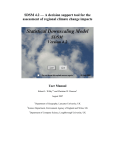
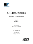
Once LARS-WG has been started and you have accepted the licence conditions (the first small
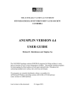
window which appears), the main menu for the weather generator appears (see Figure 3.1). The key
functions of LARS-WG are demonstrated using Debrecen, Hungary, as an example. Data for this site
Figure 3.1: The LARS-WG main window
LARS-WG: Stochastic Weather Generator
6
are included with the LARS-WG software. To quit LARS-WG at any time, simply click on the Exit
tab on the main menu.
3.1: Site Analysis
The first step in the procedure for generating daily time-series of weather data is SITE
ANALYSIS. In this process observed weather data for the site in question are analysed and two files
are produced:
1. a parameter file (*.wg), which contains the parameters required by LARS-WG to generate
synthetic weather time-series, and
2. a statistics file (*.sta) containing the seasonal frequency distributions for wet and dry series
length and for hot and cold spells, which is used in the QTest process.
These files are automatically stored in the Sitebase directory, a sub-directory located under
c:\Program Files\LARS-WG 3.0. If you wish to create a different directory and save the files there
instead, then you will need to change the locations
using the OPTIONS facility. Click on the Options
button at the top of the LARS-WG main menu, and
the window illustrated in Figure 3.2 will appear.
Check that the directory locations indicated in the
SITE ANALYSIS and GENERATOR windows
are correct. If it is necessary to amend these details
then simply click in the appropriate window and
type in the relevant information. To save these new
details and return to the main menu click on the red
Figure 3.2: The Options window, for
tick icon on the right-hand side of this window; if
changing directory location specifications.
the details are correct then simply click on the hand
icon to exit this window and return to the main menu.
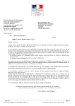
To start the SITE ANALYSIS process, click on the Analysis button on the LARS-WG main
menu. The window indicated in Figure 3.3 will appear. Here, LARS-WG requires details regarding
the directory location and name of the file containing
the site information. Illustrated in Figure 3.3 are the
details for Debrecen. To change this information you
can either click in the window and type in the
appropriate details, or you can edit the Debrecen site
information file (debr.st) to create a new file
containing the information for another site. To do this,
click on the left-hand icon illustrating a piece of paper Figure 3.3: The Site Analysis window
on which something is being written. The debr.st file which specifies the location and name of
the file containing the site information.
is then opened using Notepad (see Figure 3.4).
Figure 3.4: The debr.st file containing
site information for Debrecen (Notepad
window cropped to reduce blank space).
This file contains information about the site
(name and location), the directory path and name of
the file containing the weather data for the site,
followed by a number of ‘tags’ denoting the
organisation of the data in the weather file. To
create a new *.st file for your site, simply edit this
information appropriately and then save as a new
file (use the Save As option on the File menu in
Notepad – make sure that the file is located in the
appropriate directory). If you wish to add any
LARS-WG: Stochastic Weather Generator
7
explanatory notes to the *.st file, you can use “//” at the beginning of lines containing comments – the ‘//’
will result in these lines being ignored by the model.
The layout of the *.st file is as follows:
•
•
•
•
•
[SITE] – the station name identifier, e.g., Debrecen
[LAT, LON and ALT] – latitude, longitude and altitude for the site
[WEATHER FILES] – the directory path location and name of the file containing the observed
weather data for the site
[FORMAT] – the format of the observed weather data in the file. Here the DEBR6090.sr file
contains information for the year (YEAR), Julian day (JDAY, i.e., from 1 to 365 or 366), minimum
temperature (MIN; °C), maximum temperature (MAX; °C), precipitation (RAIN; mm) and solar
radiation (RAD; MJm-2day-1). Other tags which can be used in the format line are: DAY (day of
month), MONTH (month identifier from 1 [January] to 12 [December]) and SUN (sunshine hours).
If solar radiation is not available for a particular site, then sunshine hours may be used instead – the
weather generator automatically converts sunshine hours to solar radiation using an algorithm based
on that described in Rietveld (1978). LARS-WG will work with precipitation data alone, or with
precipitation plus any combination of the other climate variables listed above.
[END] – denoting the end of the file
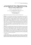
Figure 3.5: An example of
the layout of a typical file of
weather data for use in
LARS-WG. This example is
for Debrecen and is organised
according to the [FORMAT]
statement shown in Figure
3.4, i.e., Year, Julian day,
minimum then maximum
temperature, precipitation and
solar radiation.
For best results, observed weather data should be supplied for several years according to the
following recommendations:
•
•
•
•
LARS-WG will be able to simulate artificial weather data based on as little as a single year of
observed weather data. However, since the simulated weather data will be based on these
observed data, then the more data used the closer is LARS-WG likely to be able to match the true
climate for the site in question. The use of at least 20-30 years of daily weather data is
recommended. In order to be able to capture some of the less frequent climate events (e.g.,
droughts) as long an observed record as possible should be used.
The observed weather data can be contained in more than one file. Simply list the directory path
and file names in chronological order under the [WEATHER FILES] tag in the *.st file.
Each line in the data record represents a single day and the values must be in the same order for
each day according to the tags in the [FORMAT] statement in the *.st file.
The days must be in chronological order starting with the earliest record.
LARS-WG: Stochastic Weather Generator
•
•
8
The values for each day should be separated by spaces or tabs. The data should not contain blank
lines, comment lines or headers.
Missing data values should be coded -99.0.
Once the *.st and data files have been prepared then the SITE ANALYSIS process can continue.
Click on the icon indicating a graph (second from the left) in the Site Analysis window. If LARS-WG
encounters illegal data during the Site Analysis process, then it will display an error message (see
Figure 3.6(a)). Illegal data includes, for example, minimum temperature greater than maximum
temperature and negative precipitation values. You can opt to view the Error.txt file which
LARS-WG automatically creates when possible errors are located by clicking on the Yes button in the
Errors in input window which is displayed. An example of some errors deliberately contained in the
debr6090.sr data file is illustrated in Figure 3.6(b). Viewing the Error.txt file gives you the
opportunity to go back and correct the data file, if possible, before running LARS-WG. If you choose
not to view the Error.txt file or you are unable to correct the errors then simply click on No to
continue. LARS-WG will ignore the suspect data values it has identified (i.e., it will treat them as
missing values) and they will not be included in the parameter calculation process.
(a)
(b)
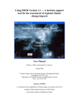
Figure 3.6: Identification of errors in
observed weather data files by LARS-WG.
(a) The Errors in input window which
appears when possible errors are identified.
(b) An example of the Error.txt file generated
when running Site Analysis for Debrecen.
LARS-WG lists the data values which are
likely to be incorrect.
Successful completion of the Site Analysis process will result in the Success window (see Figure
3.7) being displayed. Simply click on OK to be returned to the main LARS-WG screen.
If you look in the Sitebase directory under c:\Program
Files\LARS-WG 3.0 (or the relevant sub-directory if you
changed the location details using the Options facility), then you
will see that two files have been created – debrecen.sta and
debrecen.wg. The files are named according to the information
given in the [SITE] tag in the *.st file. These two files provide the
statistical characteristics of the data and parameter information
which will be used by LARS-WG to synthesise artificial weather
data in the GENERATOR process, respectively. You can open
Figure 3.7: The Success
these files using, for example, WordPad and view their contents.
window which is displayed
The layout of these files is explained as follows:
after successful completion of
Statistical characteristics: *.sta files (e.g., debrecen.sta)
the Site Analysis process.
The first few lines in this file give the site name and location
LARS-WG: Stochastic Weather Generator
9
information. This is followed by the statistical characteristics of the observed weather data. Figure
3.8(a) illustrates an excerpt from the debrecen.sta file. Each block of output in this file is preceded by
a header line describing its contents.
1. [SERIES WET AND DRY]: This block of output indicates the empirical distribution
characteristics for the length of wet and dry series of days in the observed data. This information
is given in blocks of four lines by season (i.e., winter [DJF], spring [MAM], summer [JJA] and
autumn [SON]). The first two lines of each seasonal block refer to the WET series, whilst the last
two lines represent the DRY series. As explained in Section 2, the wet and dry series are modelled
based on histograms constructed from the observed data. The histograms consist of 10 intervals
(or bins) and the cut-off points for each bin are given in the first line of each set of two lines. The
second line corresponds to the number of events in the observed data falling into each interval.
(a)
(b)
Figure 3.8: Examples of the parameter files produced by LARS-WG in the Site Analysis
process. Both files are derived from observed weather data. (a) the *.sta file which contains
statistical characteristics of the observed weather data. (b) the *.wg file which contains the
parameters used by LARS-WG to simulate artificial weather data.
LARS-WG: Stochastic Weather Generator
2.
3.
4.
5.
6.
7.
8.
9.
10
So, using debrecen.sta, it can be seen that the WET series intervals (hi) are 0≤h1<1, 1≤h2<2,
2≤h3<3, 3≤h4<4, 4≤h5<5, 5≤h6<6, 6≤h7<7, 7≤h8<8, 8≤h9<10 and 10≤h10<13, with corresponding
frequencies of occurrence of 215, 136, 70, 39, 19, 8, 10, 1, 5 and 2, respectively (see Figure
3.8(a)). Similarly, the winter DRY series intervals are 0≤h1<1, 1≤h2<3, 3≤h3<6, 6≤h4<10,
10≤h5<15, 15≤h6<22, 22≤h7<31, 31≤h8<42, 42≤h9<55 and 55≤h10<70, with corresponding
occurrence frequencies of 183, 175, 92, 43, 9, 8, 1, 0, 0 and 1, respectively. The histogram
intervals are derived from the observed data and are not pre-set. Hence, they will differ from site
to site.
[WET and DRY SERIES: mean and sd]: The following block of data describes the mean and
standard deviation, by month, of wet and dry series length. The first two lines are the mean and
standard deviation for the WET series, followed by the same information for the DRY series. The
mean indicates the average length, in days, of the appropriate series in each month, whilst the
standard deviation gives an indication of the variability of the series length in each month.
[DISTRIBUTIONS OF RAIN]: Precipitation amount is modelled in the same way as series
length, i.e., empirical distributions are derived using frequency histograms, the intervals of which
are based on the observed weather data. An empirical precipitation amount distribution is derived
for each month, resulting in the 24 lines in this block (listed from January through to December).
Each pair of lines represents the histogram intervals followed by the frequency of precipitation
occurrence within each interval.
[RAIN MONTHLY max, min, N, mean and sd]: Following the precipitation distribution
characteristics are summary precipitation statistics by month. The first two lines represent the
absolute maximum and minimum precipitation totals (mm) recorded in each month. The next line
indicates the number of years of data in the record (N; 31 for the Debrecen example), followed by
monthly mean precipitation total and standard deviation.
[MAX MONTHLY max, min, N, mean and sd]: Next are a number of statistics related to monthly
mean maximum temperature, arranged as in (4) above. These are derived by pooling the mean
maximum temperature for each month and year. The first two lines represent the extremes of
monthly mean maximum temperature, i.e., the absolute maximum and minimum monthly mean
maximum temperature values, respectively. N is the number of years of record followed by the
monthly mean maximum temperature and standard deviation (i.e., the year-to-year variation for
the month in question).
[MAX DAILY max, min, N, mean and sd]: LARS-WG also provides information about the
statistical characteristics of daily maximum temperature, derived by pooling the daily maximum
temperature values for each month and year. The first two lines represent the extremes of daily
maximum temperature, i.e., the absolute maximum and minimum daily maximum temperature
values, respectively. N is the number of days in the record (i.e., the number of days in the relevant
month multiplied by the number of years of record) and this is followed by the daily mean
maximum temperature and standard deviation (i.e., the day-to-day variation for the month in
question).
[MIN MONTHLY max, min, N, mean and sd]: As (5), but for monthly mean minimum
temperature.
[MIN DAILY max, min, N, mean and sd]: As (6), but for daily minimum temperature.
[SPELLS OF FROST and HOT TEMPERATURE]: Periods of cool and warm weather are also
modelled using empirical distributions by season. A frost is defined as a minimum temperature
less than 0°C, whilst a hot day occurs if maximum temperature exceeds 30°C. Each seasonal
block of data consists of four lines with the first line of each pair describing the histogram
intervals (spell length) and the second line the frequency of occurrence of events within each
interval, respectively. The first two lines represent frost events, whilst the last two lines relate to
hot spells.
LARS-WG: Stochastic Weather Generator
11
10. [RAD MONTHLY max, min, N, mean and sd]: Statistical characteristics of monthly mean solar
radiation (MJm-2day-1) are given. First of all, the maximum and minimum monthly mean solar
radiation values, followed by the number of years of record (N), monthly mean solar radiation and
standard deviation. These values are obtained by pooling the monthly mean solar radiation values.
11. [RAD DAILY max, min, N, mean and sd]: Finally, the statistical characteristics of daily solar
radiation are provided: maximum and minimum daily solar radiation, the number of days of
record (N), daily mean solar radiation and standard deviation. These values are obtained by
pooling the daily solar radiation values.
Weather generator parameters: *.wg files (e.g., debrecen.wg)
The *.wg files contain the statistical parameters derived from the observed weather data and used
by LARS-WG to simulate synthetic weather data (see Figure 3.8(b) for an example). This file also
starts with the site name and location followed by the parameter information in the following order:
1. [SERIES]: Monthly histogram intervals and frequency of events in these intervals for wet and dry
series length. Each block of four lines (one block for each month starting in January and ending in
December) represents wet (first pair of lines) and dry (second pair of lines) series information.
The first line in each pair corresponds to the histogram intervals, whilst the second indicates the
frequency of events within each interval.
2. [RAIN]: Histogram intervals and frequency of events in these intervals for precipitation amount
by month from January to December. The first line in each pair corresponds to the histogram
intervals, whilst the second indicates the frequency of events in each interval.
Temperature is modelled in LARS-WG by using Fourier series, i.e., the annual cycle of temperature is
described using sine and cosine curves. These curves can be constructed with information pertaining
to only a small number of parameters, i.e., the mean value, amplitude of the sine/cosine curves and
phase angle. Both maximum and minimum temperature are modelled more accurately by considering
wet and dry days separately.
3. [WET MIN]: First two lines are four Fourier coefficients, a[i] and b[i] i=1,…4, for the means of
minimum temperature on wet days and second two lines are Fourier coefficients for standard
deviations of minimum temperature on wet days.
4. [WET MAX] Fourier coefficients for the means and standard deviations of maximum temperature
on wet days.
5. [DRY MIN] Fourier coefficients for the means and standard deviations of minimum temperature
on dry days.
6. [DRY MAX] Fourier coefficients for the means and standard deviations of maximum temperature
on dry days.
The weather on a given day is related to some extent by what has happened on the previous day, e.g.,
if the previous day was hot then storage of heat energy in the soil, etc. and release of this energy over
time means that it is likely that the next day will be warm as well. This dependence on the previous
day’s weather is known as autocorrelation. LARS-WG uses an average autocorrelation value for
minimum and maximum temperature and solar radiation, derived from the observed weather data.
7. [AUTO MIN]: Average autocorrelation value for minimum temperature.
8. [AUTO MAX]: Average autocorrelation value for maximum temperature.
9. [AUTO RAD]: Average autocorrelation value for solar radiation.
Solar radiation is also modelled using empirical distributions based on frequency histograms.
Improved representation of solar radiation was obtained by modelling the solar radiation amounts
separately for wet and dry days.
10. [WET RAD]: Solar radiation amount (MJm-2day-1) on wet days by month from January to
December. Each pair of lines indicates the histogram intervals (first line) and the frequency of
events in each interval (second line). The histogram interval values are obtained from the
observed weather data and are not pre-set.
LARS-WG: Stochastic Weather Generator
12
11. [DRY RAD]: Solar radiation amount (MJm-2day-1) on dry days by month from January to
December. Each pair of lines indicates the histogram intervals (first line) and the frequency of
events in each interval (second line). The histogram interval values are obtained from the
observed weather data and are not pre-set.
3.2: QTest
Once LARS-WG has been calibrated using observed station data, the next step in the process is to
determine how well the model performs, i.e., to assess the ability of LARS-WG to simulate the
climate at the chosen site, in order to determine whether or not it is suitable for use in your
application. This can be done in two ways, either: (i) use the GENERATOR option to synthesise
daily weather data based on the information in the site parameter files and then undertake
comparisons between the observed and synthetic data ‘off-line’, or (ii) use the QTest option. Here the
QTest option will be described, with details about the GENERATOR option following in Section
3.3.
The QTest option carries out a statistical comparison of synthetic weather data generated using
LARS-WG with the parameters derived from observed weather data. In order to ensure that the
simulated data probability distributions are close to the true long-term observed distributions for the
site in question, a large number of years of simulated weather data should be generated.
To start QTest click on the QTest button on the LARS-WG main menu. A drop-down menu with
two options, Test or Compare, will appear. Both options compare the probability distributions for the
synthetic and observed data using the Chi-square goodness-of-fit test and the means and standard
deviations using the t and F tests, respectively, with the results written to the *.tst file (e.g.,
debrecen.tst) located in the Sitebase directory.
The Test option enables the user to generate synthetic data for any number of years (default 300)
based on the parameter files for the site in question. The synthetic data are then analysed and
parameter files produced containing probability distribution, mean and standard deviation
information. The file containing the synthetic data is only temporary – as soon as the parameter files
have been generated, the data file is deleted. However, there must be enough disk space on your PC to
allow generation of this data file. To run this option simply select the name of your site from the pulldown menu, insert the number of years of data you wish to generate (if different from the default
value of 100 years) and finally select the random seed number you wish to use (default is 577), as
shown in the QTest window illustrated in Figure 3.9 (left). Then click on the graph icon and the test
will be undertaken. Once it is complete, a Success window will appear and you will be asked if you
wish to view the results. Simply click on Yes or No, as desired. The results are written to the file with
extension *.tst and named after your site, e.g., for Debrecen the file is called Debrecen.tst, and is
located in the Sitebase subdirectory. The parameter files generated from the synthetic data are also
housed in this subdirectory and they are distinguished from the original parameter files calculated
from the observed station data by the ‘WG’ in the filename. For example, the original parameter files
for Debrecen are named Debrecen.sta and Debrecen.wg, whilst those derived from the synthetic data
are called DebrecenWG.sta and DebrecenWG.wg
Figure 3.9: The windows for the QTest options, Test (left) and Compare (right).
LARS-WG: Stochastic Weather Generator
13
The Compare option allows comparison of the statistics of existing *.sta parameter files. In the
Compare statistics window (see Figure 3.9, right) you simply need to fill in the appropriate file
names, with the name of the observed *.sta file in the upper window and that of the *.sta file derived
from simulated data in the lower window, e.g., debrecen.sta and debrecenWG.sta, respectively, in this
example. Click on the graph icon to start the test and once it is completed a Success window will
appear and you will be asked if you wish to view the results. Click on Yes or No as desired. The
results are written to the *.tst file located in the Sitebase directory.
3.2.1: Explanation of the *.tst file
The *.tst file contains the results of comparing the statistical characteristics of the observed data
with those of simulated data generated from the parameter files calculated from the observed data.
This file starts with the location information for the site in question. The results of the tests are then
given in the following order:
1: [SERIES: Wet/Dry – degrees of freedom, Chi-squared values and probabilities]: The quarterly
probability distributions for the length of wet and dry series are compared using the Chi-squared
goodness-of-fit test. For each season, the output is the number of degrees of freedom, the Chisquared test value and the probability that the observed and synthetic values come from the same
probability distribution.
2: [RAIN distribution – degrees of freedom, Chi-squared values and probabilities]: As (1) but for
monthly precipitation amount.
3: [RAIN MONTHLY – obs/wg mean and sd, t- and F- values and probabilities] Block of eight lines
of data following the header line. Lines 1 and 2 indicate the monthly mean precipitation totals and
standard deviations calculated from the observed data. Monthly mean totals and standard
deviations of the synthetic data are indicated in lines 3 and 4. Lines 5 and 6 illustrate the results of
the t-test which compares the mean values. Line 5 is the calculated t value and line 6 is the
associated p-value, i.e., the probability that the observed and synthetic mean values are derived
from the same population. Lines 7 and 8 indicate the results of the F-test which is used to see if
the observed and synthetic data are from normal distributions with the same variance. Line 7 is
the calculated F value and line 8 is the associated p-value.
4: [MIN MONTHLY – obs/wg mean and sd, t- and F- values and probabilities] As (3) but for
monthly minimum temperature.
5: [MIN DAILY – obs/wg mean and sd, t- and F- values and probabilities] As (3) but for daily
minimum temperature.
6: [MAX MONTHLY – obs/wg mean and sd, t- and F- values and probabilities] As (3) but for
monthly maximum temperature.
7: [MAX DAILY – obs/wg mean and sd, t- and F- values and probabilities] As (3) but for daily
maximum temperature.
8: [SPELLS: FROST/HOT – degrees of freedom, Chi-squared values and probabilities] As (1) but
for hot (maximum temperature >30°C) and cold (minimum temperature <0°C) spells. (It is
assumed that temperature is measured in degrees Celsius and not in degrees Fahrenheit.)
9: [RAD MONTHLY – obs/wg mean and sd, t- and F- values and probabilities] As (3) but for
monthly solar radiation.
10: [RAD DAILY – obs/wg mean and sd, t- and F- values and probabilities] As (3) but for daily solar
radiation.
The Chi-squared (χ2) test is usually used to compare an empirical data histogram with a probability
distribution function. In this case the χ2 test is used to compare two data histograms, i.e., that derived
using observed data with that derived using synthetic data. The data are first divided into discrete
LARS-WG: Stochastic Weather Generator
14
Figure 3.10: An example of the output from the QTest Test or Compare options. Here the
Debrecen.tst file is illustrated.
classes, or bins, and the test statistic is then calculated by counting the data values falling into each
class in relation to the computed theoretical probabilities, which in this case are calculated from the
observed data. In each class, the number of data values expected to occur according to the fitted
distribution (i.e., the observed data) is simply the probability of occurrence in that class multiplied by
the sample size, n. If the synthetic data are very close to the observed data, the expected and observed
counts will be very close for each class and the squared differences in the above equation will be very
small, yielding a small χ2. If the fit is not good, at least a few of the classes will exhibit large
discrepancies.
Meaning of the p-value and interpretation of output statistics
The χ2, t- and F- tests assume that the observed weather is a random sample from some existing
distribution, which represents the ‘true’ climate at the site. In the absence of any changes in climate,
this true distribution could be estimated accurately from observed data over a very long time period.
The simulated climate distribution is estimated from a long run of synthetic weather data
generated by LARS-WG using the parameter files output during the model calibration process (in
principle this distribution could be determined for any given site from the parameter file for the site,
although the calculation is difficult because of complex interactions between the parameters).
The statistical tests carried out in QTest look for differences between the simulated climate and
the ‘true’ climate. Each of the tests considers a particular weather statistic and compares the values
from the observed and simulated data. All of the tests calculate a p-value, which is used to accept or
reject the hypotheses that the two sets of data could have come from the same distribution (i.e., there
LARS-WG: Stochastic Weather Generator
15
is no difference between the ‘true’ and simulated climate for that variable). Therefore, a very low pvalue means that the simulated climate is unlikely to be the same as the ‘true’ climate. If the p-value is
not very low, it is plausible that the climates are the same, although statistical tests cannot prove this.
Particular weather variables for which the test process exhibits very low p-values should,
therefore, be investigated (see reasons for differences below). The level of p-value to consider
significant is subjective and depends on the importance of a very close fit for your application.
However, it is suggested that a p-value of less than 0.01 be taken as indicating the likelihood of a
substantial difference between the ‘true’ and simulated climate for that particular variable. Although
the 0.05 value is a common significance level used in statistical tests, on average 1 in 20 tests will still
be less than 0.05 even when there is no difference. For example, if a run of the generator was treated
as the observed data and was tested using the QTest option, on average 1 in 20 tests would give a pvalue less than 0.05 even though both sets of data do actually come from the same source.
Sample size also affects the likelihood of a significant p-value. The tests are more useful (are
more likely to give a significant result) with more data. A small sample size (i.e., little observed data
or a short run of simulated data) gives little information as to the ‘true’ distribution for a particular
climate variable.
Reasons for significant differences
Significant differences between simulated and observed data are likely to be due to LARS-WG
smoothing the observed data. For example, LARS-WG fits smooth curves to the average daily mean
values for minimum temperature and for maximum temperature. It does this in order to eliminate as
much as possible the random noise in the observed data in order to get closer to the actual climate for
the site. Differences are likely to be due to departures of the observed values from the smooth pattern
for the data. For example, suppose that the observed monthly maximum temperatures for January to
July for a site are:
Month
Maximum temperature (°C)
Jan
1
Feb
4
Mar
10
Apr
16
May
13
Jun
24
Jul
26
In this case, the mean maximum temperature for May does not follow the expected trend of increasing
temperatures during the first half of the year and so there is likely to be a significant difference
between the simulated and observed data for May. Possible reasons for such data and the appropriate
responses are:
•
Errors in the observed data: Correct the errors and re-run LARS-WG.
•
Random variation in the observed data: In the above example, May could have been unusually
cold in the years covered by the observed data and so the data would not be typical of the true
climate at that site. Random variations from month to month are likely to be greater when there is
less observed data. If the differences are due to such random variations, the smoothing employed
by LARS-WG will mean that the simulated weather is likely to be closer to the actual climate for
the site than the observed data and so the simulated data can be accepted. [LARS-WG assumes
that the observed climate is stationary; if there are any trends in the observed data then these need
to be removed before LARS-WG is used.]
•
Climate anomalies: The variations in the data may be due to some unusual climatic phenomenon
and so the data may actually be typical of the climate for the site. It is likely that in this case
LARS-WG will not match the climate for that part of the year. In this case, careful consideration
is needed of the effect on your application of the differences between LARS-WG and the typical
climate.
LARS-WG: Stochastic Weather Generator
16
3.3: Generator
Once LARS-WG has been calibrated using observed weather data for the site in question
(Analysis) and the performance of the weather generator has been verified (QTest), synthetic weather
data may be simulated using the Generator option. This option may be used to generate synthetic
data which have the same statistical characteristics as the observed weather data, or to generate
synthetic weather data corresponding to a scenario of climate change.
Figure 3.11: The Generator window
indicating the options available for
generating synthetic weather data.
To generate synthetic weather data click on the Generator tab on the LARS-WG main menu. The
window illustrated in Figure 3.11 will appear. Fill in the details for your site as necessary. Specify the
site name in the Site window (click on the arrow on the right-hand side of this window to obtain a
listing of the sites at which LARS-WG has been calibrated and highlight the name of your station;
Debrecen is the default), then select the appropriate Scenario file, the Scaling factor, the Number of
years to be generated and the Random seed value.
LARS-WG uses a Scenario file to determine how the weather generator parameter values should
be perturbed. If you wish to generate synthetic weather data based on the parameters derived from
observed data then you will need to use the bs.sce file (see Figure 3.12), located in the Sitebase
directory (and provided with LARS-WG). The information contained in this file tells LARS-WG that
it should not apply any changes to the parameter values and so the synthetic data generated using the
parameter files should have the same statistical characteristics as the observed data.
This bs.sce file can be edited to create a scenario file containing values corresponding to a climate
change scenario if required. Click on the Edit scenario icon (a piece of paper on which something is
being written) on the right-hand side of the Generator window and the scenario file which is
specified in the Scenario window (see Figure 3.11) will be opened in Notepad to allow edits to be
made. Remember to change the [NAME] tag so that the output file will be named appropriately to
describe the scenario you are using and remember to use the SaveAs option to save this information in
a new file with the extension *.sce, also named appropriately.
The bs.sce file contains the following information (see Figure 3.12):
1. [NAME]: This tag is used to name the output file containing the synthetic data. In this example,
the output file will be called base.sr. Simply type in the name you wish to be used to identify the
output file.
2. [DATA]: This block of data contains the information used to perturb the weather generator
parameter files. In column order from left to right we have: name of month, monthly precipitation
change (m.rain), changes in the length of the wet series (wet), changes in the length of the dry
series (dry), followed by changes in mean temperature (tem), in the standard deviation of
temperature (sd) and in mean radiation (rad), respectively.
LARS-WG uses the information in the DATA block in the following manner. The changes in
mean temperature and solar radiation are additive changes, i.e., a zero indicates that no change is to be
applied. The mean temperature change value for a given month is applied to both the minimum and
LARS-WG: Stochastic Weather Generator
17
Figure 3.12: The bs.sce file, used to generate synthetic weather data with the same statistical
characteristics as the observed weather data used to calibrate LARS-WG.
maximum temperature values for that month. For example, if the tem parameter is set to 1.5 for
January, then 1.5°C will be added to each of the daily minimum and maximum temperature values
simulated by LARS-WG for January. Changes in monthly precipitation, length of wet and dry spells
and temperature standard deviation are multiplicative, i.e., they are expressed as ratios
(future/baseline value), and so a value of 1 indicates no change. A value greater (less) than 1 indicates
increases (decreases) in the relevant parameter. LARS-WG multiplies each value that it chooses for
precipitation, length of wet and dry series and temperature variability by the corresponding values in
this file. For example, setting the wet series parameter for January equal to 1.5 will result in the
lengths of each of the wet series chosen by LARS-WG in January being multiplied by 1.5.
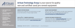
Changes in precipitation, mean temperature and solar radiation are at the monthly time scale,
whilst changes in wet and dry series length and temperature variability must be derived from daily
data. An example of a climate change scenario file is given in Figure 3.13. In this example, changes in
the average values of total monthly precipitation (m.rain), mean temperature (tem) and radiation (rad)
were calculated from changes in monthly precipitation, mean temperature and solar radiation between
the 1961-1990 baseline period and the 2035-2064 period of the HadCM2 greenhouse gas only climate
change experiment. For example, the m.rain value of 1.23 for January means that monthly
precipitation in January for 2035-2064 is 1.23 times higher than monthly precipitation for 1961-1990,
the tem value of 1.80 for January means that mean temperature in January for 2035-2064 is 1.80°C
warmer than that for 1961-1990. Changes for wet and dry spells and changes in temperature standard
deviation were derived from daily HadCM2 model output.
Changing wet and dry spell lengths without making changes to any of the other variables in the
parameter file will usually lead to changes in monthly mean precipitation amount, mean temperature
LARS-WG: Stochastic Weather Generator
18
Figure 3.13: An example of a climate change scenario file. The changes indicated in this file
are derived from the HadCM2 greenhouse gas only experiment for the years 2035-2064 (i.e.,
centred on 2050) calculated with respect to the 1961-1990 baseline period.
and solar radiation, since these values are conditioned on the precipitation status of the day in
question. This unexpected response to changing the precipitation parameters has also been observed
in stochastic weather generators based on Markov chain processes (Katz, 1996). LARS-WG performs
self-adjustment of precipitation amount, temperature and solar radiation in order to keep the changes
specified for these variables as close as possible to those given in the scenario file. The adjustment
factors are based on the generation of a large number of years (i.e., 1000) of data and so the changes
in the different climate variables will only approach the values in the scenario file if a large amount of
data is generated.
Once you have selected your site and set up the appropriate scenario files there are three further
options to be completed. The first is the Scaling factor. This factor can be used if you have
implemented a climate change scenario for a particular future time period, say 2100, and you want to
obtain data for an earlier time period without having to create a scenario file for this earlier time
period. The Scaling factor allows you to do this by assuming that the changes in climate over time are
linear. So for example, if you have already created a scenario file for 2100 and you wish to obtain data
for 2030 using this file, then you would set the Scaling value to 0.3. This is a ‘quick and dirty’ way of
generating scenarios for other time periods and it is not a method, which should generally be used,
particularly since global climate model output is now available, usually continuously, from about
1900 to 2100. Using the default value of 1 means that no scaling is applied.
Select the Number of years you wish to generate by typing in the appropriate number in this
window. There is no limit to the number of years of data that LARS-WG can generate – the only
constraint is the amount of disk space available (100 years of data requires approximately 1.5MB of
LARS-WG: Stochastic Weather Generator
19
disk space).
Finally you need to select the Random seed value. The stochastic component of LARS-WG is
controlled by a random number seed. There are a number of pre-set random seeds available – click on
the arrow on the right-hand side of this window to obtain a listing of these values. It is advised that
you use these pre-set random seed values, but if you wish to select your own random seed value then
you should choose a prime number within the range of 500 to 1500. You can generate a number of
different realisations of weather time series by selecting a different random seed value. These
realisations will all have the same statistical characteristics, but they will differ on a day-to-day basis.
If you repeat a run with the same seed value then you will get exactly the same data as in the earlier
run. However, if you change the seed value then the data will be different on a day-to-day basis,
although the statistical characteristics will be the same. Remember to change the [NAME] tag in the
*.sce file you are using in order to distinguish between the output data files produced using different
random number seeds – if you do not do this then the output file will simply be overwritten. Different
weather sequences may have different effects in your application and so, as with any stochastic
modelling process, the application may need to be run several times with the different weather
sequences. The longer the time period of simulated weather that is used, the more it will cover the full
range of possible weather events. Long weather sequences are usually required when assessing risk.
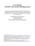
Figure 3.14 illustrates the format of a typical file of synthetic weather data generated by
LARS-WG. The first two columns are the year number and the day number, respectively. The format
of the rest of the file will mirror the format of the input file. For example, if your observed weather
data file was in the order MAX, MIN, RAIN, RAD, then this will be the format of the synthetic
weather data generated in the output file. If you have used SUN as an input climate variable it is
converted to solar radiation and RAD will be output.
Figure 3.14: An example of the file format of generated data. The first two columns
represent year number and day number, respectively, and the next four columns indicate
minimum then maximum temperature, precipitation and solar radiation, respectively.
This format corresponds to that of the input file used in the calibration process.
LARS-WG: Stochastic Weather Generator
20
3.3.1: Creating climate scenarios from GCM output.
One of the main uses of stochastic weather generators is in the generation of daily weather data
representing scenarios of climate change. Most climate change scenarios are derived from the output
of global climate models (GCMs), with changes in the different climate variables expressed on a
monthly, rather than a daily, time scale. The simplest method of applying climate change scenarios is
to perturb an observed daily time series by monthly changes in the relevant climate variable. For
example, if January temperatures are projected to increase by 2°C, then all daily January values in the
observed record would be increased by 2°C, i.e., the new perturbed time series will have exactly the
same variability as the original, but the January temperatures will be 2°C warmer. A stochastic
weather generator, however, allows the generation of synthetic daily weather data which will
incorporate these changes, but which will be different from the original time series on a day-to-day
basis, although the statistical characteristics will be (almost) identical. It also allows changes in
climate variability to be incorporated, if desired, and not just changes in mean values.
The following section outlines the procedure for constructing a scenario of climate change to be
used with LARS-WG to generate synthetic daily weather data. If you wish to incorporate changes in
climate variability, then you will need to have access to daily GCM output. If you are interested only
in generating daily data from monthly changes in climate, then you will need only scenarios of
climate change at the monthly time scale. The following process assumes that perturbations are being
made to all four of the climate variables which LARS-WG can generate – if you are using a subset of
these variables, then obviously you need only climate change information for the relevant variables.
1. Extract daily precipitation, maximum and minimum temperature and solar radiation data from the
appropriate global climate model experiment for the baseline period (usually 1961-1990) and the
relevant future time period (e.g., 2040-2069 to represent the 2050s). The simplest method is to use
data from the grid box within which your station is located. Although some GCMs do not have
365 days in the model year (e.g., HadCM2 and HadCM3 have 12 months each of 30 days in
length to give a year total of 360 days) it is not necessary to represent these days as missing
values – LARS-WG will automatically recognise that some days are absent and will use missing
values to represent these days.
2. Set up the *.st file, which provides LARS-WG with site and directory location information, and
the *.sr files which contain the model data. Use the latitude and longitude values for the centre of
the appropriate grid box as the site location. Make sure you select [SITE] tags in the *.st file
which will enable you to easily identify the parameter files for the two time periods. You must
make sure that the files are named differently otherwise the parameter files will be overwritten.
3. Undertake Site Analysis using the daily global climate model data for both the baseline and
future time periods. This will result in two *.wg and two *.sta parameter files corresponding to
the two time periods you have chosen.
4. To incorporate variability into your scenarios, you need to calculate the relative change in wet and
dry series lengths. Calculate the mean of the empirical distributions for wet and dry spell length
from the baseline and future time period *.wg files. To do this, calculate the mid-point value for
each histogram bin by averaging the bin boundary values. Multiply this mid-point value by the
number of events in this bin to obtain an average number of days in this category. Do this for each
histogram bin and sum these values together to get an approximation for the total number of wet
(or dry) days. Calculate the total number of events by simply adding together the number of
events in each bin. To calculate the mean value for the distribution, divide the sum of the wet (or
dry) days by the total number of events. For the January wet series indicated in Figure 3.8(b) for
Debrecen.wg, this would result in the following values:
The mid-point values are: 0.5, 1.5, 2.5, 3.5, 4.5, 5.5, 6.5, 7.5, 9.0 and 11.5.
Average number of days in each bin: 39 (0.5×78), 69(1.5×46), 67.5, 49, 18, 22, 26, 7.5, 9 and
LARS-WG: Stochastic Weather Generator
21
23, totalling 330. The total number of events is 181. The average length of a January wet spell
is therefore 1.82 days (330/181). Do this for wet and dry series for each month and for the
baseline and future time periods. To calculate the relative change in length of wet (or dry)
series divide the average length of the series in the future time period by the average length of
the series in the baseline time period, e.g., length2040-2069/length1961-1990. You now have relative
changes for each series for each month.
5. You also need to calculate the relative change in mean temperature standard deviation for each
month. This can be derived from GCM daily mean temperature data, or it may be necessary to
determine daily mean temperature by averaging daily maximum and minimum temperature GCM
output. Pool the daily temperature values for each month and calculate the standard deviation (so,
for example, for a model which has 31 days in January and for which you are using 30 years of
data you would have a total of 930 data values [30 years × 31 days] from which you would
calculate the standard deviation). Do this for both the baseline and future time periods. Calculate
the relative change in temperature standard deviation by dividing the standard deviation for the
future time period by the standard deviation for the baseline time period, e.g.,
st.dev.2040-2069/st.dev.1961-1990.
6. You also need mean changes in precipitation amount, mean temperature and solar radiation for
each month. To calculate the monthly mean changes in precipitation amount you need to refer to
the *.sta files generated using daily GCM data for the baseline and future time periods. Go to the
block of data in these files which has the header [RAIN MONTHLY max, min, N, mean, sd] and
extract the values corresponding to mean precipitation amount (5th line below this header). The
relative change in monthly precipitation amount is simply the value for the future period divided
by that for the baseline period, e.g., precip. amount2040-2069/precip. amount1961-1990. Alternatively,
you may use corresponding monthly precipitation scenario values (i.e., the relative change in
monthly precipitation between the future and baseline periods) since these should be identical to
the changes derived from the daily precipitation data.
For monthly mean changes in mean temperature and solar radiation, you need the monthly mean
change in these values between the future and baseline periods. For solar radiation, these values
may also be derived from the *.sta files. Simply scroll down to the block of data headed by the
[RAD MONTHLY max, min, N, mean and sd] tag in each *.sta file and calculate the difference
between the future and baseline periods. Remember that LARS-WG requires the solar radiation
data to be in units of MJm-2day-1. Most GCM output is in units of Wm-2, so you will need to
convert the data into MJm-2day-1 by multiplying the Wm-2 values by 0.0864.
You now have the information required to construct the climate change scenario file and thus to
generate daily weather data representing future scenario conditions. A worked example of creating a
climate change scenario using Rothamsted, UK, as an example is illustrated below.
1. Daily weather data for Rothamsted for the period 1961-1990 were converted into the correct
format for use in LARS-WG and the model calibrated using the Analysis option. Thirty years of
synthetic weather data were then generated using the Generator option.
2. Daily maximum and minimum temperature and precipitation data were extracted from the
greenhouse gas + sulphate aerosol climate change experiment undertaken with the HadCM2 GCM
for the grid box within which Rothamsted is located (referred to as Box 139). Thirty years of data
were extracted for two time periods, 1961-1990 (baseline) and 2035-2064 (to represent 2050).
Two data files (*.sr) were prepared in the correct format for input into LARS-WG.
LARS-WG: Stochastic Weather Generator
22
Figure 3.15: Examples of the *.st files used with the HadCM2 daily data. Left: for 1961-1990;
Right: for 2035-2064. (Note: Figures cropped to remove blank space).
3. Figure 3.15 illustrates examples of the *.st files used with the HadCM2 daily data and
LARS-WG. (Note that although the [SITE] tags are the same for the 1961-1990 and 2035-2064
time periods, the parameter files for each time period were moved to different directory locations
immediately after their generation and so they were not overwritten.)
4. Site Analysis was undertaken using the daily HadCM2 data for the two time periods, 1961-1990
and 2035-2064 and *.wg and *.sta files produced.
5. The relative changes in wet and dry spell length were calculated from the empirical distributions
described in the *.wg parameter files (see Figure 3.16). As an example, here we will calculate the
relative change in January wet spell length. If you look at the box139.wg file corresponding to the
1961-1990 HadCM2 data (Figure 3.16, top) then you would calculate the mean wet spell length in
January in the following manner:
First of all calculate the mid-point values for the histogram bins by averaging adjacent bin
boundary values. In this example, the following values result: 0.5, 2.0, 4.5, 8.0, 13.0, 20.0, 29.0,
40.0, 52.0 and 68.0. To obtain the average number of wet days in each category, multiply the midpoint values by the number of events in that category. Here the results are: 1.5 (0.5×3), 16.0
(2.0×8), 63.0 (4.5×14), 88.0, 208.0, 160.0, 261.0, 360.0, 364.0, 340.0. Sum these values and then
divide the result by the total number of events (1861.5/90) to obtain the average January wet spell
length for the 1961-1990 HadCM2 daily data (20.68).
Follow exactly the same procedure for the 2035-2064 data illustrated in Figure 3.16 (bottom) to
obtain the average January wet spell length for this time period (19.01). The relative change in
wet spell length in this month is then simply wet-spell2035-2064/wet-spell1961-1990 (19.01/20.68), i.e.,
0.919. Follow the same procedure to calculate the relative change in wet and dry series length for
each month.
6. The daily mean temperature data for both time periods from the HadCM2 experiment were
derived by averaging daily maximum and minimum temperature data from the same experiment.
For each month and time period all daily values were pooled and the mean and standard
deviations calculated. The change in monthly mean temperature was calculated by subtracting the
monthly mean temperature values for 1961-1990 from the monthly mean values for the
LARS-WG: Stochastic Weather Generator
23
2035-2064 period. The relative change in temperature standard deviation was calculated simply
by dividing the 2035-2064 standard deviation by that for 1961-1990. This process resulted in the
values illustrated below:
Month
Mean temperature
change (°C)
Change in
standard deviation
J
1.4
F
2.0
M
0.5
A
0.7
M
1.4
1.06
0.97 1.09 1.11 0.96
J
0.7
J
1.7
A
2.6
0.97 0.94 1.20
S
1.9
O
1.9
1.13 1.09
N
1.9
D
1.0
1.09 1.06
7. The monthly mean changes in precipitation and solar radiation may be obtained from the *.sta
files (see Figure 3.17). For precipitation scroll down to the block of data headed by the tag [RAIN
MONTHLY max, min, N, mean, sd] in the baseline and future *.sta files and then calculate the
relative change between the future and baseline periods. For example, from Figure 3.17, monthly
total precipitation for January, February and March in 1961-1990 is 69.8mm, 56.3mm and
63.4mm, respectively. Corresponding values for the 2035-2064 period are 68.7mm, 61.4mm and
58.4mm, respectively. Hence, the relative changes in monthly precipitation for January, February
and March are 0.984 (68.7/69.8), 1.091 (61.4/56.3) and 0.921 (58.4/63.4), respectively. For solar
radiation simply scroll down to the block of data preceded by the tag [RAD MONTHLY max,
min, N, mean and sd] in each time period *.sta file and calculate the simple difference between
the future and baseline periods.
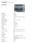
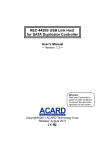
8. From the results of (7) and above a scenario file was prepared for Rothamsted (see Figure 3.18).
This scenario file can be used to generate any number of years of data representing the climate of
the 2050s.
LARS-WG: Stochastic Weather Generator
24
Figure 3.16: The *.wg parameter files obtained by calibrating LARS-WG with daily GCM
data from HadCM2 for the periods 1961-1990 (top) and 2035-2064 (bottom). The section of
the files illustrated indicates the wet and dry series empirical distribution information which is
used to calculate the relative change in wet and dry spell length.
LARS-WG: Stochastic Weather Generator
25
Figure 3.18: The scenario file for Rothamsted, indicating mean changes in
precipitation, mean temperature and solar radiation and relative changes in wet and
dry spell length and temperature standard deviation.
LARS-WG: Stochastic Weather Generator
26
3.4: Spatial interpolation of LARS-WG
A methodology for the spatial interpolation of LARS-WG parameters has also been developed for
Great Britain (Semenov & Brooks, 1998), and this option is described in this section although it is not
activated in the version of the software currently available. The INTERPOLATION option allows the
LARS-WG parameters to be interpolated to any location in Great Britain, even where observed weather
data are unavailable – the resulting parameter file can then be used to generate synthetic weather data.
The Great Britain database had been derived from two data sets of observed weather: (i) 138 sites
in Great Britain with daily values of minimum and maximum temperature, precipitation and radiation
or sunshine hours over relatively long periods of between 20 and 40 years. This data set was used to
produce parameter files for all 138 sites. (ii) a 1961 – 1990 database of mean monthly precipitation
for 2376 stations and of minimum and maximum temperature for 623 stations. This data set was used
to calculate spline interpolation functions for monthly precipitation and minimum and maximum
temperatures as a function of latitude, longitude and elevation.
The spatial interpolation procedure of LARS-WG combines global and local interpolation.
Similarity in the nature of the distributions of the weather variables for nearby sites is expected since
these sites will normally be subject to the same basic type of weather on each day. However,
systematic differences can occur particularly if the sites are at significantly different elevations, with
precipitation tending to increase and temperature tending to decrease with elevation. The interpolation
procedure devised consists of an initial local interpolation in which the weighted average of the
weather generator parameters for three neighbouring sites from the database are calculated. The
precipitation and temperature distributions of the target site were adjusted for the site elevation.
Precipitation-elevation and temperature-elevation relationships were obtained from global
interpolation of monthly average precipitation and temperature by thin plate spline functions using
elevation as an independent variable in addition to the geographical coordinates (Hutchinson, 1995).
The parameters for precipitation and temperature at the target site were then adjusted based on the
mean values predicted by the spline functions. If the interpolated site coincides with one of existing
sites from database, the actual parameter file will be used.
•
Run the INTERPOLATION option to interpolate LARS-WG parameters to any given site in
Great Britain, specified in (longitude, latitude, altitude) coordinates. Enter the name of the site, its
latitude and longitude (in degrees) and its altitude (in metres) in the dialogue box. As a result the
interpolated parameter file (*.wg) will be created in the Interpolation Result directory, as
specified in OPTIONS, along with a *.int file which contains the monthly values for total
precipitation, minimum and maximum temperature predicted by the spline functions. This file can
then be used to generate daily weather series. The Interpolation Data directory includes the
database of about 150 parameters files for sites in Great Britain as well as parameters of spline
functions for monthly total precipitation, minimum and maximum temperature.
The support of Dr Mike Hutchinson, Australian National University, in providing the ANUSPLIN
program and discussing interpolation issues is gratefully acknowledged.
4:
REFERENCES
Bailey, N.T.J. (1964): The Elements of Stochastic Processes, Wiley: New York.
Chia, E. & Hutchinson, M.F. (1991): The beta distribution as a probability model for daily cloud
duration. Agric. For. Meterol. 56, 195-208.
Downing, T.E., Harrison, P.A., Butterfield, R.E. & Lonsdale, K.G. (Eds) (2000): Climate Change,
Climatic Variability and Agriculture in Europe: An Integrated Assessment. Environmental Change
Institute, University of Oxford.
LARS-WG: Stochastic Weather Generator
27
Harrison, P.A., Butterfield, R.E. & Downing, T.E. (Eds) (1995): Climate Change and Agriculture in
Europe: Assessment of Impacts and Adaptations. Environmental Change Unit Research Report
No. 9, Environmental Change Unit, University of Oxford.
Hutchinson, M.F. (1995): Interpolating mean rainfall using thin plate smoothing splines. Inter. J.
Geograph. Inform. Systems 9, 385-403.
Katz, R.W. (1996): Use of conditional stochastic models to generate climate change scenarios.
Climatic Change 32, 237-255.
Racsko P., Szeidl L. & Semenov M. (1991): A serial approach to local stochastic weather models.
Ecological Modelling 57, 27-41.
Richardson C.W. (1981). Stochastic Simulation of Daily Precipitation, Temperature, and Solar Radiation.
Water Resources Research, 17,182-190.
Richardson, C.W. & Wright, D.A. (1984): WGEN: A model for generating daily weather variables. US
Department of Agriculture, Agricultural Research Service, ARS-8, USDA, Washington, DC.
Rietveld M.R. (1978): A new method for the estimating the regression coefficients in the formula relating
solar radiation to sunshine. Agricultural and Forest Meteorology 19, 243-252.
Semenov M.A. & Barrow E.M. (1997): Use of a stochastic weather generator in the development of
climate change scenarios. Climatic Change 35, 397-414.
Semenov M.A., Brooks R.J., Barrow E.M. & Richardson C.W (1998): Comparison of the WGEN and
LARS-WG stochastic weather generators in diverse climates. Climate Research 10, 95-107.
Semenov M.A. & Brooks R.J. (1999): Spatial interpolation of the LARS-WG stochastic weather
generator in Great Britain. Climate Research 11, 137-148.
5:
ADDRESS FOR COMMUNICATIONS
Dr Mikhail Semenov
Rothamsted Research
Harpenden, Hertfordshire
AL5 2JQ
UNITED KINGDOM
Tel: + 44 (0) 1582 763133 ext. 2395
E-mail: [email protected]
Web site: http://www.iacr.bbsrc.ac.uk/mas-models/larswg.html
6:
LICENCE AGREEMENT
An individual academic can use LARS-WG for research purposes. The use of the LARS-WG as a part
of a research project requires a licence agreement.
LARS-WG CANNOT be used for any commercial purposes.