Download A ROOT Guide For Beginners “Diving Into ROOT”

A ROOT Guide For Beginners
“Diving Into ROOT”
2
Contents
1 Motivation and Introduction
5
2 ROOT Basics
7
2.1
ROOT as calculator . . . . . . . . . . . . . . . . . . . . . . . . . . . . . . . . . . . . . . . . . . . . . . . . .
7
2.2
Learn C++ at the ROOT prompt . . . . . . . . . . . . . . . . . . . . . . . . . . . . . . . . . . . . . . . . .
8
2.3
ROOT as function plotter . . . . . . . . . . . . . . . . . . . . . . . . . . . . . . . . . . . . . . . . . . . . . .
9
2.4
Controlling ROOT . . . . . . . . . . . . . . . . . . . . . . . . . . . . . . . . . . . . . . . . . . . . . . . . . . 11
2.5
Plotting Measurements . . . . . . . . . . . . . . . . . . . . . . . . . . . . . . . . . . . . . . . . . . . . . . . . 11
2.6
Histograms in ROOT . . . . . . . . . . . . . . . . . . . . . . . . . . . . . . . . . . . . . . . . . . . . . . . . . 13
2.7
Interactive ROOT . . . . . . . . . . . . . . . . . . . . . . . . . . . . . . . . . . . . . . . . . . . . . . . . . . 15
2.8
ROOT Beginners’ FAQ . . . . . . . . . . . . . . . . . . . . . . . . . . . . . . . . . . . . . . . . . . . . . . . 15
2.8.1
ROOT type declarations for basic data types . . . . . . . . . . . . . . . . . . . . . . . . . . . . . . . 17
2.8.2
Configure ROOT at start-up . . . . . . . . . . . . . . . . . . . . . . . . . . . . . . . . . . . . . . . . 17
2.8.3
ROOT command history
2.8.4
ROOT Global Pointers
. . . . . . . . . . . . . . . . . . . . . . . . . . . . . . . . . . . . . . . . . . 17
. . . . . . . . . . . . . . . . . . . . . . . . . . . . . . . . . . . . . . . . . . . 17
3 ROOT Macros
19
3.1
General Remarks on ROOT macros
3.2
A more complete example . . . . . . . . . . . . . . . . . . . . . . . . . . . . . . . . . . . . . . . . . . . . . . 20
3.3
Summary of Visual effects . . . . . . . . . . . . . . . . . . . . . . . . . . . . . . . . . . . . . . . . . . . . . . 22
3.4
. . . . . . . . . . . . . . . . . . . . . . . . . . . . . . . . . . . . . . . . 19
3.3.1
Colours and Graph Markers . . . . . . . . . . . . . . . . . . . . . . . . . . . . . . . . . . . . . . . . . 22
3.3.2
Arrows and Lines . . . . . . . . . . . . . . . . . . . . . . . . . . . . . . . . . . . . . . . . . . . . . . . 22
3.3.3
Text . . . . . . . . . . . . . . . . . . . . . . . . . . . . . . . . . . . . . . . . . . . . . . . . . . . . . . 24
Interpretation and Compilation . . . . . . . . . . . . . . . . . . . . . . . . . . . . . . . . . . . . . . . . . . . 24
3.4.1
Compile a Macro with ACLiC . . . . . . . . . . . . . . . . . . . . . . . . . . . . . . . . . . . . . . . . 24
3.4.2
Compile a Macro with the Compiler . . . . . . . . . . . . . . . . . . . . . . . . . . . . . . . . . . . . 24
4 Graphs
27
4.1
Read Graph Points from File . . . . . . . . . . . . . . . . . . . . . . . . . . . . . . . . . . . . . . . . . . . . 27
4.2
Polar Graphs . . . . . . . . . . . . . . . . . . . . . . . . . . . . . . . . . . . . . . . . . . . . . . . . . . . . . 29
4.3
2D Graphs
4.4
Multiple graphs . . . . . . . . . . . . . . . . . . . . . . . . . . . . . . . . . . . . . . . . . . . . . . . . . . . . 33
. . . . . . . . . . . . . . . . . . . . . . . . . . . . . . . . . . . . . . . . . . . . . . . . . . . . . . 29
3
4
CONTENTS
5 Histograms
35
5.1
Your First Histogram
. . . . . . . . . . . . . . . . . . . . . . . . . . . . . . . . . . . . . . . . . . . . . . . . 35
5.2
Add and Divide Histograms . . . . . . . . . . . . . . . . . . . . . . . . . . . . . . . . . . . . . . . . . . . . . 36
5.3
Two-dimensional Histograms . . . . . . . . . . . . . . . . . . . . . . . . . . . . . . . . . . . . . . . . . . . . 39
5.4
Multiple histograms . . . . . . . . . . . . . . . . . . . . . . . . . . . . . . . . . . . . . . . . . . . . . . . . . 42
6 Functions and Parameter Estimation
45
6.1
Fitting Functions to Pseudo Data . . . . . . . . . . . . . . . . . . . . . . . . . . . . . . . . . . . . . . . . . . 45
6.2
Toy Monte Carlo Experiments . . . . . . . . . . . . . . . . . . . . . . . . . . . . . . . . . . . . . . . . . . . . 47
7 File I/O and Parallel Analysis
51
7.1
Storing ROOT Objects . . . . . . . . . . . . . . . . . . . . . . . . . . . . . . . . . . . . . . . . . . . . . . . . 51
7.2
N-tuples in ROOT . . . . . . . . . . . . . . . . . . . . . . . . . . . . . . . . . . . . . . . . . . . . . . . . . . 52
7.2.1
Storing simple N-tuples . . . . . . . . . . . . . . . . . . . . . . . . . . . . . . . . . . . . . . . . . . . 52
7.2.2
Reading N-tuples . . . . . . . . . . . . . . . . . . . . . . . . . . . . . . . . . . . . . . . . . . . . . . . 53
7.2.3
Storing Arbitrary N-tuples . . . . . . . . . . . . . . . . . . . . . . . . . . . . . . . . . . . . . . . . . 54
7.2.4
Processing N-tuples Spanning over Several Files
7.2.5
For the advanced user: Processing trees with a selector script . . . . . . . . . . . . . . . . . . . . . . 56
7.2.6
For power-users: Multi-core processing with PROOF lite . . . . . . . . . . . . . . . . . . . . . . . . 59
7.2.7
Optimisation Regarding N-tuples . . . . . . . . . . . . . . . . . . . . . . . . . . . . . . . . . . . . . . 60
8 ROOT in Python
8.1
61
PyROOT . . . . . . . . . . . . . . . . . . . . . . . . . . . . . . . . . . . . . . . . . . . . . . . . . . . . . . . 61
8.1.1
8.2
. . . . . . . . . . . . . . . . . . . . . . . . . . . . . 55
More Python- less C++ . . . . . . . . . . . . . . . . . . . . . . . . . . . . . . . . . . . . . . . . . . . 63
Custom code: from C++ to Python . . . . . . . . . . . . . . . . . . . . . . . . . . . . . . . . . . . . . . . . 63
9 Concluding Remarks
65
10 References
67
Abstract
ROOT is a software framework for data analysis and I/O: a powerful tool to cope with the demanding tasks typical of
state of the art scientific data analysis. Among its prominent features are an advanced graphical user interface, ideal
for interactive analysis, an interpreter for the C++ programming language, for rapid and efficient prototyping and a
persistency mechanism for C++ objects, used also to write every year petabytes of data recorded by the Large Hadron
Collider experiments. This introductory guide illustrates the main features of ROOT which are relevant for the typical
problems of data analysis: input and plotting of data from measurements and fitting of analytical functions.
Chapter 1
Motivation and Introduction
Welcome to data analysis!
Comparison of measurements to theoretical models is one of the standard tasks in experimental physics. In the most simple
case, a “model” is just a function providing predictions of measured data. Very often, the model depends on parameters.
Such a model may simply state “the current I is proportional to the voltage U ”, and the task of the experimentalist
consists of determining the resistance, R, from a set of measurements.
As a first step, a visualisation of the data is needed. Next, some manipulations typically have to be applied, e.g. corrections
or parameter transformations. Quite often, these manipulations are complex ones, and a powerful library of mathematical
functions and procedures should be provided - think for example of an integral or peak-search or a Fourier transformation
applied to an input spectrum to obtain the actual measurement described by the model.
One specialty of experimental physics are the inevitable uncertaintes affecting each measurement, and visualisation tools
have to include these. In subsequent analysis, the statistical nature of the errors must be handled properly.
As the last step, measurements are compared to models, and free model parameters need to be determined in this process.
See Figure 1.1 for an example of a function (model) fit to data points. Several standard methods are available, and a data
analysis tool should provide easy access to more than one of them. Means to quantify the level of agreement between
measurements and model must also be available.
Quite often, the data volume to be analyzed is large - think of fine-granular measurements accumulated with the aid of
computers. A usable tool therefore must contain easy-to-use and efficient methods for storing and handling data.
In Quantum mechanics, models typically only predict the probability density function (“pdf”) of measurements depending
on a number of parameters, and the aim of the experimental analysis is to extract the parameters from the observed
distribution of frequencies at which certain values of the measurement are observed. Measurements of this kind require
means to generate and visualize frequency distributions, so-called histograms, and stringent statistical treatment to extract
the model parameters from purely statistical distributions.
Simulation of expected data is another important aspect in data analysis. By repeated generation of “pseudo-data”, which
are analysed in the same manner as intended for the real data, analysis procedures can be validated or compared. In many
cases, the distribution of the measurement errors is not precisely known, and simulation offers the possibility to test the
effects of different assumptions.
A powerful software framework addressing all of the above requirements is ROOT, an open source project coordinated by
the European Organisation for Nuclear Research, CERN in Geneva.
ROOT is very flexible and provides both a programming interface to use in own applications and a graphical user interface
for interactive data analysis. The purpose of this document is to serve as a beginners guide and provides extendable
examples for your own use cases, based on typical problems addressed in student labs. This guide will hopefully lay the
ground for more complex applications in your future scientific work building on a modern, state-of the art tool for data
analysis.
This guide in form of a tutorial is intended to introduce you quickly to the ROOT package. This goal will be accomplished
using concrete examples, according to the “learning by doing” principle. Also because of this reason, this guide cannot
cover all the complexity of the ROOT package. Nevertheless, once you feel confident with the concepts presented in the
following chapters, you will be able to appreciate the ROOT Users Guide (The ROOT Users Guide 2015) and navigate
5
6
CHAPTER 1. MOTIVATION AND INTRODUCTION
through the Class Reference (The ROOT Reference Guide 2013) to find all the details you might be interested in. You can
even look at the code itself, since ROOT is a free, open-source product. Use these documents in parallel to this tutorial!
The ROOT Data Analysis Framework itself is written in and heavily relies on the C++ programming language: some
knowledge about C++ is required. Jus take advantage from the immense available literature about C++ if you do not have
any idea of what this language is about.
ROOT is available for many platforms (Linux, Mac OS X, Windows. . . ), but in this guide we will implicitly assume that
you are using Linux. The first thing you need to do with ROOT is install it, don’t you ? Obtaining the latest ROOT
version is straightforward. Just seek the “Pro” version on this webpage http://root.cern.ch/downloading-root. You will
find precompiled versions for the different architectures, or the ROOT source code to compile yourself. Just pick up the
flavour you need and follow the installation instructions.
Let’s dive into ROOT!
Chapter 2
ROOT Basics
Now that you have installed ROOT, what’s this interactive shell thing you’re running ? It’s like this: ROOT leads a double
life. It has an interpreter for macros (Cling (“What Is Cling” 2015)) that you can run from the command line or run like
applications. But it is also an interactive shell that can evaluate arbitrary statements and expressions. This is extremely
useful for debugging, quick hacking and testing. Let us first have a look at some very simple examples.
2.1
ROOT as calculator
You can even use the ROOT interactive shell in lieu of a calculator! Launch the ROOT interactive shell with the command
> root
on your Linux box. The prompt should appear shortly:
root [0]
and let’s dive in with the steps shown here:
root [0] 1+1
(int)2
root [1] 2*(4+2)/12.
(double) 1.000000e+00
root [2] sqrt(3.)
(double) 1.732051e+00
root [3] 1 > 2
(bool) false
root [4] TMath::Pi()
(Double_t) 3.141593e+00
root [5] TMath::Erf(.2)
(Double_t) 2.227026e-01
Not bad. You can see that ROOT offers you the possibility not only to type in C++ statements, but also advanced
mathematical functions, which live in the TMath namespace.
Now let’s do something more elaborated. A numerical example with the well known geometrical series:
root [6]
(double)
root [7]
(int) 30
root [8]
double x=.5
5.000000e-01
int N=30
double geom_series=0
7
8
CHAPTER 2. ROOT BASICS
(double) 0.000000e+00
root [9] for (int i=0;i<N;++i)geom_series+=TMath::Power(x,i)
root [10] TMath::Abs(geom_series - (1-TMath::Power(x,N-1))/(1-x))
(Double_t) 1.862645e-09
Here we made a step forward. We even declared variables and used a for control structure. Note that there are some
subtle differences between Cling and the standard C++ language. You do not need the “;” at the end of line in interactive
mode – try the difference e.g. using the command at line root [6].
2.2
Learn C++ at the ROOT prompt
Behind the ROOT prompt there is an interpreter based on a real compiler toolkit: LLVM. It is therefore possible to
exercise many features of C++ and the standard library. For example in the following snippet we define a lambda function,
a vector and we sort it in different ways:
root
root
root
root
0
3
5
4
1
2
root
root
0
1
2
3
4
5
root
root
5
4
3
2
1
0
[0]
[1]
[2]
[3]
using doubles = std::vector<double>;
auto pVec = [](const doubles& v){for (auto&& x:v) cout << x << endl;};
doubles v{0,3,5,4,1,2};
pVec(v);
[4] std::sort(v.begin(),v.end());
[5] pVec(v);
[6] std::sort(v.begin(),v.end(),[](double a, double b){return a>b;});
[7] pVec(v);
Or, if you prefer random number generation:
root [0] std::default_random_engine generator;
root [1] std::normal_distribution<double> distribution(0.,1.);
root [2] distribution(generator)
(std::normal_distribution<double>::result_type) -1.219658e-01
root [3] distribution(generator)
(std::normal_distribution<double>::result_type) -1.086818e+00
root [4] distribution(generator)
(std::normal_distribution<double>::result_type) 6.842899e-01
Impressive isn’t it?
2.3. ROOT AS FUNCTION PLOTTER
2.3
9
ROOT as function plotter
Using one of ROOT’s powerful classes, here TF1,1 will allow us to display a function of one variable, x. Try the following:
root [11] TF1 f1("f1","sin(x)/x",0.,10.);
root [12] f1.Draw();
f1 is an instance of a TF1 class, the arguments are used in the constructor; the first one of type string is a name to be
entered in the internal ROOT memory management system, the second string type parameter defines the function, here
sin(x)/x, and the two parameters of type double define the range of the variable x. The Draw() method, here without
any parameters, displays the function in a window which should pop up after you typed the above two lines.
A slightly extended version of this example is the definition of a function with parameters, called [0], [1] and so on in
the ROOT formula syntax. We now need a way to assign values to these parameters; this is achieved with the method
SetParameter(<parameter_number>,<parameter_value>) of class TF1. Here is an example:
root
root
root
root
[13]
[14]
[15]
[16]
TF1 f2("f2","[0]*sin([1]*x)/x",0.,10.);
f2.SetParameter(0,1);
f2.SetParameter(1,1);
f2.Draw();
Of course, this version shows the same results as the initial one. Try playing with the parameters and plot the function again.
The class TF1 has a large number of very useful methods, including integration and differentiation. To make full use of this
and other ROOT classes, visit the documentation on the Internet under http://root.cern.ch/drupal/content/reference-guide.
Formulae in ROOT are evaluated using the class TFormula, so also look up the relevant class documentation for examples,
implemented functions and syntax.
You should definitely download this guide to your own system to have it at you disposal whenever you need it.
To extend a little bit on the above example, consider a more complex function you would like to define. You can also do
this using standard C or C++ code.
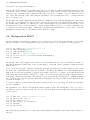
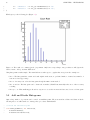
Consider the example below, which calculates and displays the interference pattern produced by light falling on a multiple
slit. Please do not type in the example below at the ROOT command line, there is a much simpler way: Make sure you
have the file slits.C on disk, and type root slits.C in the shell. This will start root and make it read the “macro”
slits.C, i.e. all the lines in the file will be executed one after the other.
1
2
3
// Example drawing the interference pattern of light
// falling on a grid with n slits and ratio r of slit
// width over distance between slits.
4
5
auto pi = TMath::Pi();
6
7
8
9
10
// function code in C
double single(double *x, double *par) {
return pow(sin(pi*par[0]*x[0])/(pi*par[0]*x[0]),2);
}
11
12
13
14
double nslit0(double *x,double *par){
return pow(sin(pi*par[1]*x[0])/sin(pi*x[0]),2);
}
15
16
17
18
double nslit(double *x, double *par){
return single(x,par) * nslit0(x,par);
}
19
20
21
// This is the main program
void slits() {
1 All
ROOT classes’ names start with the letter T. A notable exception is RooFit. In this context all classes’ names are of the form Roo*.
10
CHAPTER 2. ROOT BASICS
float r,ns;
22
23
// request user input
cout << "slit width / g ? ";
scanf("%f",&r);
cout << "# of slits? ";
scanf("%f",&ns);
cout <<"interference pattern for "<< ns
<<" slits, width/distance: "<<r<<endl;
24
25
26
27
28
29
30
31
// define function and set options
TF1 *Fnslit = new TF1("Fnslit",nslit,-5.001,5.,2);
Fnslit->SetNpx(500);
32
33
34
35
// set parameters, as read in above
Fnslit->SetParameter(0,r);
Fnslit->SetParameter(1,ns);
36
37
38
39
40
41
42
}
// draw the interference pattern for a grid with n slits
Fnslit->Draw();
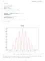
Figure 2.1: Output of slits.C with parameters 0.2 and 2.
The example first asks for user input, namely the ratio of slit width over slit distance, and the number of slits. After
entering this information, you should see the graphical output as is shown in Figure 2.1.
2.4. CONTROLLING ROOT
11
This is a more complicated example than the ones we have seen before, so spend some time analysing it carefully, you
should have understood it before continuing. Let us go through it in detail:
Lines 7-18 define the necessary functions in C++ code, split into three separate functions, as suggested by the problem
considered. The full interference pattern is given by the product of a function depending on the ratio of the width and
distance of the slits, and a second one depending on the number of slits. More important for us here is the definition of the
interface of these functions to make them usable for the ROOT class TF1: the first argument is the pointer to x, the second
one points to the array of parameters.
The main program starts at line 21 with the definition of a function slits() of type void. After asking for user input, a
ROOT function is defined using the C-type function given in the beginning. We can now use all methods of the TF1 class
to control the behaviour of our function – nice, isn’t it ?
If you like, you can easily extend the example to also plot the interference pattern of a single slit, using function double
single, or of a grid with narrow slits, function double nslit0, in TF1 instances.
Here, we used a macro, some sort of lightweight program, that the interpreter distributed with ROOT, Cling, is able to
execute. This is a rather extraordinary situation, since C++ is not natively an interpreted language! There is much more to
say: chapter is indeed dedicated to macros.
2.4
Controlling ROOT
One more remark at this point: as every command you type into ROOT is usually interpreted by Cling, an “escape
character” is needed to pass commands to ROOT directly. This character is the dot at the beginning of a line:
root [1] .<command>
This is a selection of the most common commands.
• quit root, simply type .q
• obtain a list of commands, use .?
• access the shell of the operating system, type .!<OS_command>; try, e.g. .!ls or .!pwd
• execute a macro, enter .x <file_name>; in the above example, you might have used .x slits.C at the ROOT
prompt
• load a macro, type .L <file_name>; in the above example, you might instead have used the command .L slits.C
followed by the function call slits();. Note that after loading a macro all functions and procedures defined therein
are available at the ROOT prompt.
• compile a macro, type .L <file_name>+; ROOT is able to manage for you the C++ compiler behind the scenes
and to produce machine code starting from your macro. One could decide to compile a macro in order to obtain
better performance or to get nearer to the production environment.
Use .help at the prompt to inspect the full list.
2.5
Plotting Measurements
To display measurements in ROOT, including errors, there exists a powerful class TGraphErrors with different types of
constructors. In the example here, we use data from the file ExampleData.txt in text format:
root [0] TGraphErrors gr("ExampleData.txt");
root [1] gr.Draw("AP");
12
CHAPTER 2. ROOT BASICS
Figure 2.2: Visualisation of data points with errors using the class TGraphErrors.
2.6. HISTOGRAMS IN ROOT
13
You should see the output shown in Figure 2.2.
Make sure the file ExampleData.txt is available in the directory from which you started ROOT. Inspect this file now with
your favourite editor, or use the command less ExampleData.txt to inspect the file, you will see that the format is very
simple and easy to understand. Lines beginning with # are ignored. It is very convenient to add some comments about the
type of data. The data itself consist of lines with four real numbers each, representing the x- and y- coordinates and their
errors of each data point.
The argument of the method Draw("AP") is important here. Behind the scenes, it tells the TGraphPainter class to show
the axes and to plot markers at the x and y positions of the specified data points. Note that this simple example relies on
the default settings of ROOT, concerning the size of the canvas holding the plot, the marker type and the line colours
and thickness used and so on. In a well-written, complete example, all this would need to be specified explicitly in order
to obtain nice and well readable results. A full chapter on graphs will explain many more of the features of the class
TGraphErrors and its relation to other ROOT classes in much more detail.
2.6
Histograms in ROOT
Frequency distributions in ROOT are handled by a set of classes derived from the histogram class TH1, in our case TH1F.
The letter F stands for “float”, meaning that the data type float is used to store the entries in one histogram bin.
root
root
root
root
root
root
[0]
[1]
[2]
[3]
[4]
[5]
TF1 efunc("efunc","exp([0]+[1]*x)",0.,5.);
efunc.SetParameter(0,1);
efunc.SetParameter(1,-1);
TH1F h("h","example histogram",100,0.,5.);
for (int i=0;i<1000;i++) {h.Fill(efunc.GetRandom());}
h.Draw();
The first three lines of this example define a function, an exponential in this case, and set its parameters. In line 3 a
histogram is instantiated, with a name, a title, a certain number of bins (100 of them, equidistant, equally sized) in the
range from 0 to 5.
We use yet another new feature of ROOT to fill this histogram with data, namely pseudo-random numbers generated with
the method TF1::GetRandom, which in turn uses an instance of the ROOT class TRandom created when ROOT is started.
Data is entered in the histogram at line 4 using the method TH1F::Fill in a loop construct. As a result, the histogram
is filled with 1000 random numbers distributed according to the defined function. The histogram is displayed using the
method TH1F::Draw(). You may think of this example as repeated measurements of the life time of a quantum mechanical
state, which are entered into the histogram, thus giving a visual impression of the probability density distribution. The
plot is shown in Figure 2.3.
Note that you will not obtain an identical plot when executing the lines above, depending on how the random number
generator is initialised.
The class TH1F does not contain a convenient input format from plain text files. The following lines of C++ code do the job.
One number per line stored in the text file “expo.dat” is read in via an input stream and filled in the histogram until end
of file is reached.
root
root
root
root
root
root
[1]
[2]
[3]
[4]
[5]
[6]
TH1F h("h","example histogram",100,0.,5.);
ifstream inp; double x;
inp.open("expo.dat");
while (inp >> x) { h.Fill(x); }
h.Draw();
inp.close();
Histograms and random numbers are very important tools in statistical data analysis, a whole chapter will be dedicated to
this topic.
14
CHAPTER 2. ROOT BASICS
Figure 2.3: Visualisation of a histogram filled with exponentially distributed, random numbers.
2.7. INTERACTIVE ROOT
2.7
15
Interactive ROOT
Look at one of your plots again and move the mouse across. You will notice that this is much more than a static picture,
as the mouse pointer changes its shape when touching objects on the plot. When the mouse is over an object, a right-click
opens a pull-down menu displaying in the top line the name of the ROOT class you are dealing with, e.g. TCanvas for the
display window itself, TFrame for the frame of the plot, TAxis for the axes, TPaveText for the plot name. Depending on
which plot you are investigating, menus for the ROOT classes TF1, TGraphErrors or TH1F will show up when a right-click
is performed on the respective graphical representations. The menu items allow direct access to the members of the various
classes, and you can even modify them, e.g. change colour and size of the axis ticks or labels, the function lines, marker
types and so on. Try it!
Figure 2.4: Interactive ROOT panel for setting function parameters.
You will probably like the following: in the output produced by the example slits.C, right-click on the function line and
select “SetLineAttributes”, then left-click on “Set Parameters”. This gives access to a panel allowing you to interactively
change the parameters of the function, as shown in Figure 2.4. Change the slit width, or go from one to two and then
three or more slits, just as you like. When clicking on “Apply”, the function plot is updated to reflect the actual value of
the parameters you have set.
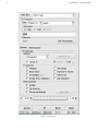
Another very useful interactive tool is the FitPanel, available for the classes TGraphErrors and TH1F. Predefined fit
functions can be selected from a pull-down menu, including “gaus”, “expo” and “pol0” - “pol9” for Gaussian and
exponential functions or polynomials of degree 0 to 9, respectively. In addition, user-defined functions using the same
syntax as for functions with parameters are possible.
After setting the initial parameters, a fit of the selected function to the data of a graph or histogram can be performed and
the result displayed on the plot. The fit panel is shown in Figure 2.5. The fit panel has a number of control options to
select the fit method, fix or release individual parameters in the fit, to steer the level of output printed on the console, or
to extract and display additional information like contour lines showing parameter correlations. As function fitting is of
prime importance in any kind of data analysis, this topic will again show up later.
If you are satisfied with your plot, you probably want to save it. Just close all selector boxes you opened previously and
select the menu item Save as... from the menu line of the window. It will pop up a file selector box to allow you to
choose the format, file name and target directory to store the image. There is one very noticeable feature here: you can
store a plot as a root macro! In this macro, you find the C++ representation of all methods and classes involved in
generating the plot. This is a valuable source of information for your own macros, which you will hopefully write after
having worked through this tutorial.
Using ROOT’s interactive capabilities is useful for a first exploration of possibilities. Other ROOT classes you will encounter
in this tutorial have such graphical interfaces. We will not comment further on this, just be aware of the existence of
ROOT’s interactive features and use them if you find them convenient. Some trial-and-error is certainly necessary to find
your way through the huge number of menus and parameter settings.
2.8
ROOT Beginners’ FAQ
At this point of the guide, some basic questions could have already come to your mind. We will try to clarify some of them
with further explanations in the following.
16
CHAPTER 2. ROOT BASICS
Figure 2.5: Fit Panel.
2.8. ROOT BEGINNERS’ FAQ
2.8.1
17
ROOT type declarations for basic data types
In the official ROOT documentation, you find special data types replacing the normal ones, e.g. Double_t, Float_t or
Int_t replacing the standard double, float or int types. Using the ROOT types makes it easier to port code between
platforms (64/32 bit) or operating systems (windows/Linux), as these types are mapped to suitable ones in the ROOT
header files. If you want adaptive code of this type, use the ROOT type declarations. However, usually you do not need
such adaptive code, and you can safely use the standard C type declarations for your private code, as we did and will do
throughout this guide. If you intend to become a ROOT developer, however, you better stick to the official coding rules!
2.8.2
Configure ROOT at start-up
The behaviour of a ROOT session can be tailored with the options in the .rootrc file. Examples of the tunable parameters
are the ones related to the operating and window system, to the fonts to be used, to the location of start-up files. At
start-up, ROOT looks for a .rootrc file in the following order:
• ./.rootrc //local directory
• $HOME/.rootrc //user directory
• $ROOTSYS/etc/system.rootrc //global ROOT directory
If more than one .rootrc files are found in the search paths above, the options are merged, with precedence local, user,
global. The parsing and interpretation of this file is handled by the ROOT class TEnv. Have a look to its documentation if
you need such rather advanced features. The file .rootrc defines the location of two rather important files inspected at
start-up: rootalias.C and rootlogon.C. They can contain code that needs to be loaded and executed at ROOT startup.
rootalias.C is only loaded and best used to define some often used functions. rootlogon.C contains code that will be
executed at startup: this file is extremely useful for example to pre-load a custom style for the plots created with ROOT.
This is done most easily by creating a new TStyle object with your preferred settings, as described in the class reference
guide, and then use the command gROOT->SetStyle("MyStyleName"); to make this new style definition the default one.
As an example, have a look in the file rootlogon.C coming with this tutorial. Another relevant file is rootlogoff.C that
it called when the session is finished.
2.8.3
ROOT command history
Every command typed at the ROOT prompt is stored in a file .root_hist in your home directory. ROOT uses this file
to allow for navigation in the command history with the up-arrow and down-arrow keys. It is also convenient to extract
successful ROOT commands with the help of a text editor for use in your own macros.
2.8.4
ROOT Global Pointers
All global pointers in ROOT begin with a small “g”. Some of them were already implicitly introduced (for example in the
section Configure ROOT at start-up). The most important among them are presented in the following:
• gROOT: the gROOT variable is the entry point to the ROOT system. Technically it is an instance of the TROOT class.
Using the gROOT pointer one has access to basically every object created in a ROOT based program. The TROOT
object is essentially a container of several lists pointing to the main ROOT objects.
• gStyle: By default ROOT creates a default style that can be accessed via the gStyle pointer. This class includes
functions to set some of the following object attributes.
–
–
–
–
–
–
Canvas
Pad
Histogram axis
Lines
Fill areas
Text
18
CHAPTER 2. ROOT BASICS
–
–
–
–
Markers
Functions
Histogram Statistics and Titles
etc . . .
• gSystem: An instance of a base class defining a generic interface to the underlying Operating System, in our case
TUnixSystem.
• gInterpreter: The entry point for the ROOT interpreter. Technically an abstraction level over a singleton instance
of TCling.
At this point you have already learnt quite a bit about some basic features of ROOT.
Please move on to become an expert!
Chapter 3
ROOT Macros
You know how other books go on and on about programming fundamentals and finally work up to building a complete,
working program ? Let’s skip all that. In this guide, we will describe macros executed by the ROOT C++ interpreter
Cling.
It is relatively easy to compile a macro, either as a pre-compiled library to load into ROOT, or as a stand-alone application,
by adding some include statements for header file or some “dressing code” to any macro.
3.1
General Remarks on ROOT macros
If you have a number of lines which you were able to execute at the ROOT prompt, they can be turned into a ROOT
macro by giving them a name which corresponds to the file name without extension. The general structure for a macro
stored in file MacroName.C is
void MacroName() {
<
...
your lines of C++ code
...
}
>
The macro is executed by typing
> root MacroName.C
at the system prompt, or executed using .x
> root
root [0] .x MacroName.C
at the ROOT prompt. or it can be loaded into a ROOT session and then be executed by typing
root [0].L MacroName.C
root [1] MacroName();
at the ROOT prompt. Note that more than one macro can be loaded this way, as each macro has a unique name in the
ROOT name space. A small set of options can help making your plot nicer.
gROOT->SetStyle("Plain");
// set plain TStyle
gStyle->SetOptStat(111111); // draw statistics on plots,
// (0) for no output
19
20
CHAPTER 3. ROOT MACROS
gStyle->SetOptFit(1111);
gStyle->SetPalette(57);
gStyle->SetOptTitle(0);
...
//
//
//
//
draw fit results on plot,
(0) for no ouput
set color map
suppress title box
Next, you should create a canvas for graphical output, with size, subdivisions and format suitable to your needs, see
documentation of class TCanvas:
TCanvas c1("c1","<Title>",0,0,400,300); // create a canvas, specify position and size in pixels
c1.Divide(2,2); //set subdivisions, called pads
c1.cd(1); //change to pad 1 of canvas c1
These parts of a well-written macro are pretty standard, and you should remember to include pieces of code like in the
examples above to make sure your plots always look as you had intended.
Below, in section Interpretation and Compilation, some more code fragments will be shown, allowing you to use the system
compiler to compile macros for more efficient execution, or turn macros into stand-alone applications linked against the
ROOT libraries.
3.2
A more complete example
Let us now look at a rather complete example of a typical task in data analysis, a macro that constructs a graph with
errors, fits a (linear) model to it and saves it as an image. To run this macro, simply type in the shell:
> root macro1.C
The code is built around the ROOT class TGraphErrors, which was already introduced previously. Have a look at it in
the class reference guide, where you will also find further examples. The macro shown below uses additional classes, TF1 to
define a function, TCanvas to define size and properties of the window used for our plot, and TLegend to add a nice legend.
For the moment, ignore the commented include statements for header files, they will only become important at the end in
section Interpretation and Compilation.
1
2
3
// Builds a graph with errors, displays it and saves it as
// image. First, include some header files
// (not necessary for Cling)
4
5
6
7
8
9
10
11
#include
#include
#include
#include
#include
#include
#include
"TCanvas.h"
"TROOT.h"
"TGraphErrors.h"
"TF1.h"
"TLegend.h"
"TArrow.h"
"TLatex.h"
12
13
14
15
16
17
18
19
20
21
void macro1(){
// The values and the errors on the Y axis
const int n_points=10;
double x_vals[n_points]=
{1,2,3,4,5,6,7,8,9,10};
double y_vals[n_points]=
{6,12,14,20,22,24,35,45,44,53};
double y_errs[n_points]=
{5,5,4.7,4.5,4.2,5.1,2.9,4.1,4.8,5.43};
22
23
// Instance of the graph
3.2. A MORE COMPLETE EXAMPLE
21
TGraphErrors graph(n_points,x_vals,y_vals,nullptr,y_errs);
graph.SetTitle("Measurement XYZ;lenght [cm];Arb.Units");
24
25
26
// Make the plot estetically better
graph.SetMarkerStyle(kOpenCircle);
graph.SetMarkerColor(kBlue);
graph.SetLineColor(kBlue);
27
28
29
30
31
// The canvas on which we'll draw the graph
auto mycanvas = new TCanvas();
32
33
34
// Draw the graph !
graph.DrawClone("APE");
35
36
37
// Define a linear function
TF1 f("Linear law","[0]+x*[1]",.5,10.5);
// Let's make the funcion line nicer
f.SetLineColor(kRed); f.SetLineStyle(2);
// Fit it to the graph and draw it
graph.Fit(&f);
f.DrawClone("Same");
38
39
40
41
42
43
44
45
// Build and Draw a legend
TLegend leg(.1,.7,.3,.9,"Lab. Lesson 1");
leg.SetFillColor(0);
graph.SetFillColor(0);
leg.AddEntry(&graph,"Exp. Points");
leg.AddEntry(&f,"Th. Law");
leg.DrawClone("Same");
46
47
48
49
50
51
52
53
// Draw an arrow on the canvas
TArrow arrow(8,8,6.2,23,0.02,"|>");
arrow.SetLineWidth(2);
arrow.DrawClone();
54
55
56
57
58
// Add some text to the plot
TLatex text(8.2,7.5,"#splitline{Maximum}{Deviation}");
text.DrawClone();
59
60
61
62
63
64
}
mycanvas->Print("graph_with_law.pdf");
65
66
67
68
int main(){
macro1();
}
Let’s comment it in detail:
• Line 13 : the name of the principal function (it plays the role of the “main” function in compiled programs) in the
macro file. It has to be the same as the file name without extension.
• Line 24-25 : instance of the TGraphErrors class. The constructor takes the number of points and the pointers to the
arrays of x values, y values, x errors (in this case none, represented by the NULL pointer) and y errors. The second
line defines in one shot the title of the graph and the titles of the two axes, separated by a “;”.
• Line 28-30 : These three lines are rather intuitive right ? To understand better the enumerators for colours and styles
see the reference for the TColor and TMarker classes.
• Line 33 : the canvas object that will host the drawn objects. The “memory leak” is intentional, to make the object
existing also out of the macro1 scope.
22
CHAPTER 3. ROOT MACROS
• Line 36 : the method DrawClone draws a clone of the object on the canvas. It has to be a clone, to survive after the
scope of macro1, and be displayed on screen after the end of the macro execution. The string option “APE” stands
for:
– A imposes the drawing of the Axes.
– P imposes the drawing of the graph’s markers.
– E imposes the drawing of the graph’s error bars.
• Line 39 : define a mathematical function. There are several ways to accomplish this, but in this case the constructor
accepts the name of the function, the formula, and the function range.
• Line 41 : maquillage. Try to give a look to the line styles at your disposal visiting the documentation of the TLine
class.
• Line 43 : fits the f function to the graph, observe that the pointer is passed. It is more interesting to look at the
output on the screen to see the parameters values and other crucial information that we will learn to read at the end
of this guide.
• Line 44 : again draws the clone of the object on the canvas. The “Same” option avoids the cancellation of the already
drawn objects, in our case, the graph. The function f will be drawn using the same axis system defined by the
previously drawn graph.
• Line 47-52 : completes the plot with a legend, represented by a TLegend instance. The constructor takes as parameters
the lower left and upper right corners coordinates with respect to the total size of the canvas, assumed to be 1,
and the legend header string. You can add to the legend the objects, previously drawn or not drawn, through the
addEntry method. Observe how the legend is drawn at the end: looks familiar now, right ?
• Line 55-57 : defines an arrow with a triangle on the right hand side, a thickness of 2 and draws it.
• Line 60-61 : interpret a Latex string which hast its lower left corner located in the specified coordinate. The
#splitline{}{} construct allows to store multiple lines in the same TLatex object.
• Line 63 : save the canvas as image. The format is automatically inferred from the file extension (it could have been
eps, gif, . . . ).
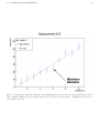
Let’s give a look to the obtained plot in Figure 3.1. Beautiful outcome for such a small bunch of lines, isn’t it ?
3.3
3.3.1
Summary of Visual effects
Colours and Graph Markers
We have seen that to specify a colour, some identifiers like kWhite, kRed or kBlue can be specified for markers, lines,
arrows etc. The complete summary of colours is represented by the ROOT “colour wheel”. To know more about the full
story, refer to the online documentation of TColor.
ROOT provides several graphics markers types. Select the most suited symbols for your plot among dots, triangles, crosses
or stars. An alternative set of names for the markers is available.
3.3.2
Arrows and Lines
The macro line 55 shows how to define an arrow and draw it. The class representing arrows is TArrow, which inherits
from TLine. The constructors of lines and arrows always contain the coordinates of the endpoints. Arrows also foresee
parameters to specify their shapes. Do not underestimate the role of lines and arrows in your plots. Since each plot should
contain a message, it is convenient to stress it with additional graphics primitives.
3.3. SUMMARY OF VISUAL EFFECTS
23
Figure 3.1: Your first plot with data points, a fit of an analytical function, a legend and some additional information in the
form of graphics primitives and text. A well formatted plot, clear for the reader is crucial to communicate the relevance of
your results to the reader.
24
3.3.3
CHAPTER 3. ROOT MACROS
Text
Also text plays a fundamental role in making the plots self-explanatory. A possibility to add text in your plot is provided
by the TLatex class. The objects of this class are constructed with the coordinates of the bottom-left corner of the text
and a string which contains the text itself. The real twist is that ordinary Latex mathematical symbols are automatically
interpreted, you just need to replace the “\” by a “#”.
If “\” is used as control character , then the TMathText interface is invoked. It provides the plain TeX syntax and allow to
access character’s set like Russian and Japenese.
3.4
Interpretation and Compilation
As you observed, up to now we heavily exploited the capabilities of ROOT for interpreting our code, more than compiling
and then executing. This is sufficient for a wide range of applications, but you might have already asked yourself “how can
this code be compiled ?”. There are two answers.
3.4.1
Compile a Macro with ACLiC
ACLiC will create for you a compiled dynamic library for your macro, without any effort from your side, except the
insertion of the appropriate header files in lines 5–11. In this example, they are already included. To generate an object
library from the macro code, from inside the interpreter type (please note the “+”):
root [1] .L macro1.C+
Once this operation is accomplished, the macro symbols will be available in memory and you will be able to execute it
simply by calling from inside the interpreter:
root [2] macro1()
3.4.2
Compile a Macro with the Compiler
A plethora of excellent compilers are available, both free and commercial. We will refer to the GCC compiler in the following.
In this case, you have to include the appropriate headers in the code and then exploit the root-config tool for the automatic
settings of all the compiler flags. root-config is a script that comes with ROOT; it prints all flags and libraries needed
to compile code and link it with the ROOT libraries. In order to make the code executable stand-alone, an entry point
for the operating system is needed, in C++ this is the procedure int main();. The easiest way to turn a ROOT macro
code into a stand-alone application is to add the following “dressing code” at the end of the macro file. This defines the
procedure main, the only purpose of which is to call your macro:
int main() {
ExampleMacro();
return 0;
}
To create a stand-alone program from a macro called ExampleMacro.C, simply type
> g++ -o ExampleMacro ExampleMacro.C `root-config --cflags --libs`
and execute it by typing
> ./ExampleMacro
3.4. INTERPRETATION AND COMPILATION
25
This procedure will, however, not give access to the ROOT graphics, as neither control of mouse or keyboard events nor
access to the graphics windows of ROOT is available. If you want your stand-alone application have display graphics
output and respond to mouse and keyboard, a slightly more complex piece of code can be used. In the example below, a
macro ExampleMacro_GUI is executed by the ROOT class TApplication. As a additional feature, this code example offers
access to parameters eventually passed to the program when started from the command line. Here is the code fragment:
void StandaloneApplication(int argc, char** argv) {
// eventually, evaluate the application parameters argc, argv
// ==>> here the ROOT macro is called
ExampleMacro_GUI();
}
// This is the standard "main" of C++ starting
// a ROOT application
int main(int argc, char** argv) {
TApplication app("ROOT Application", &argc, argv);
StandaloneApplication(app.Argc(), app.Argv());
app.Run();
return 0;
}
Compile the code with
> g++ -o ExampleMacro_GUI ExampleMacro_GUI `root-config --cflags --libs`
and execute the program with
> ./ExampleMacro_GUI
26
CHAPTER 3. ROOT MACROS
Chapter 4
Graphs
In this Chapter we will learn how to exploit some of the functionalities ROOT provides to display data exploiting the class
TGraphErrors, which you already got to know previously.
4.1
Read Graph Points from File
The fastest way in which you can fill a graph with experimental data is to use the constructor which reads data points and
their errors from an ASCII file (i.e. standard text) format:
TGraphErrors(const char *filename,
const char *format="%lg %lg %lg %lg", Option_t *option="");
The format string can be:
• "%lg %lg" read only 2 first columns into X,Y
• "%lg %lg %lg" read only 3 first columns into X,Y and EY
• "%lg %lg %lg %lg" read only 4 first columns into X,Y,EX,EY
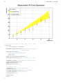
This approach has the nice feature of allowing the user to reuse the macro for many different data sets. Here is an example
of an input file. The nice graphic result shown is produced by the macro below, which reads two such input files and uses
different options to display the data points.
# Measurement of Friday 26 March
# Experiment 2 Physics Lab
1
2
3
4
5
6
7
8
9
10
6
12
14
20
22
24
35
45
44
53
5
5
4.7
4.5
4.2
5.1
2.9
4.1
4.8
5.43
27
28
CHAPTER 4. GRAPHS
// Reads the points from a file and produces a simple graph.
int macro2(){
auto c=new TCanvas();c->SetGrid();
TGraphErrors graph_expected("./macro2_input_expected.txt",
"%lg %lg %lg");
graph_expected.SetTitle(
"Measurement XYZ and Expectation;"
"lenght [cm];"
"Arb.Units");
graph_expected.SetFillColor(kYellow);
graph_expected.DrawClone("E3AL"); // E3 draws the band
TGraphErrors graph("./macro2_input.txt","%lg %lg %lg");
graph.SetMarkerStyle(kCircle);
graph.SetFillColor(0);
graph.DrawClone("PESame");
// Draw the Legend
TLegend leg(.1,.7,.3,.9,"Lab. Lesson 2");
leg.SetFillColor(0);
leg.AddEntry(&graph_expected,"Expected Points");
leg.AddEntry(&graph,"Measured Points");
leg.DrawClone("Same");
}
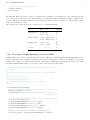
graph.Print();
return 0;
4.2. POLAR GRAPHS
29
In addition to the inspection of the plot, you can check the actual contents of the graph with the TGraph::Print() method
at any time, obtaining a printout of the coordinates of data points on screen. The macro also shows us how to print
a coloured band around a graph instead of error bars, quite useful for example to represent the errors of a theoretical
prediction.
4.2
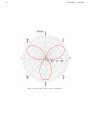
Polar Graphs
With ROOT you can profit from rather advanced plotting routines, like the ones implemented in the TPolarGraph, a class
to draw graphs in polar coordinates. You can see the example macro in the following and the resulting Figure is 4.2:
1
// Builds a polar graph in a square Canvas.
2
3
4
5
6
7
8
9
10
11
12
13
14
15
16
17
18
19
void macro3(){
auto c = new TCanvas("myCanvas","myCanvas",600,600);
Double_t rmin=0.;
Double_t rmax=TMath::Pi()*6.;
const Int_t npoints=1000;
Double_t r[npoints];
Double_t theta[npoints];
for (Int_t ipt = 0; ipt < npoints; ipt++) {
r[ipt] = ipt*(rmax-rmin)/npoints+rmin;
theta[ipt] = TMath::Sin(r[ipt]);
}
TGraphPolar grP1 (npoints,r,theta);
grP1.SetTitle("A Fan");
grP1.SetLineWidth(3);
grP1.SetLineColor(2);
grP1.DrawClone("L");
}
A new element was added on line 4, the size of the canvas: it is sometimes optically better to show plots in specific canvas
sizes.
4.3
2D Graphs
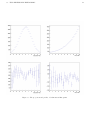
Under specific circumstances, it might be useful to plot some quantities versus two variables, therefore creating a bidimensional graph. Of course ROOT can help you in this task, with the TGraph2DErrors class. The following macro
produces a bi-dimensional graph representing a hypothetical measurement, fits a bi-dimensional function to it and draws it
together with its x and y projections. Some points of the code will be explained in detail. This time, the graph is populated
with data points using random numbers, introducing a new and very important ingredient, the ROOT TRandom3 random
number generator using the Mersenne Twister algorithm (Matsumoto 1997).
1
2
3
4
5
// Create, Draw and fit a TGraph2DErrors
void macro4(){
gStyle->SetPalette(kBird);
const double e = 0.3;
const int nd = 500;
6
7
8
9
10
11
12
13
TRandom3 my_random_generator;
TF2 f2("f2",
"1000*(([0]*sin(x)/x)*([1]*sin(y)/y))+200",
-6,6,-6,6);
f2.SetParameters(1,1);
TGraph2DErrors dte(nd);
// Fill the 2D graph
30
CHAPTER 4. GRAPHS
Figure 4.1: The graph of a fan obtained with ROOT.
4.3. 2D GRAPHS
14
15
16
17
18
19
20
21
22
23
24
25
26
27
28
29
30
31
32
33
34
35
36
37
38
39
40
41
42
43
44
45
46
47
48
49
50
}
31
double rnd, x, y, z, ex, ey, ez;
for (Int_t i=0; i<nd; i++) {
f2.GetRandom2(x,y);
// A random number in [-e,e]
rnd = my_random_generator.Uniform(-e,e);
z = f2.Eval(x,y)*(1+rnd);
dte.SetPoint(i,x,y,z);
ex = 0.05*my_random_generator.Uniform();
ey = 0.05*my_random_generator.Uniform();
ez = fabs(z*rnd);
dte.SetPointError(i,ex,ey,ez);
}
// Fit function to generated data
f2.SetParameters(0.7,1.5); // set initial values for fit
f2.SetTitle("Fitted 2D function");
dte.Fit(&f2);
// Plot the result
auto c1 = new TCanvas();
f2.SetLineWidth(1);
f2.SetLineColor(kBlue-5);
TF2
*f2c = (TF2*)f2.DrawClone("Surf1");
TAxis *Xaxis = f2c->GetXaxis();
TAxis *Yaxis = f2c->GetYaxis();
TAxis *Zaxis = f2c->GetZaxis();
Xaxis->SetTitle("X Title"); Xaxis->SetTitleOffset(1.5);
Yaxis->SetTitle("Y Title"); Yaxis->SetTitleOffset(1.5);
Zaxis->SetTitle("Z Title"); Zaxis->SetTitleOffset(1.5);
dte.DrawClone("P0 Same");
// Make the x and y projections
auto c_p= new TCanvas("ProjCan",
"The Projections",1000,400);
c_p->Divide(2,1);
c_p->cd(1);
dte.Project("x")->Draw();
c_p->cd(2);
dte.Project("y")->Draw();
Let’s go through the code, step by step to understand what is going on:
• Line 3 : This sets the palette colour code to a much nicer one than the default. Comment this line to give it a try.
This article gives more details about colour map choice.
• Line 7 : The instance of the random generator. You can then draw out of this instance random numbers distributed
according to different probability density functions, like the Uniform one at lines 27-29. See the on-line documentation
to appreciate the full power of this ROOT feature.
• Line 8 : You are already familiar with the TF1 class. This is its two-dimensional version. At line 16 two random
numbers distributed according to the TF2 formula are drawn with the method TF2::GetRandom2(double& a,
double&b).
• Line 27-29 : Fitting a 2-dimensional function just works like in the one-dimensional case, i.e. initialisation of parameters
and calling of the Fit() method.
• Line 34 : The Surf1 option draws the TF2 objects (but also bi-dimensional histograms) as coloured surfaces with a
wire-frame on three-dimensional canvases. See Figure 4.3.
• Line 35-40 : Retrieve the axis pointer and define the axis titles.
• Line 41 : Draw the cloud of points on top of the coloured surface.
32
CHAPTER 4. GRAPHS
• Line 43-49 : Here you learn how to create a canvas, partition it in two sub-pads and access them. It is very handy to
show multiple plots in the same window or image.
Figure 4.2: A dataset fitted with a bidimensional function visualised as a colored surface.
4.4. MULTIPLE GRAPHS
4.4
33
Multiple graphs
The class TMultigraph allows to manipulate a set of graphs as a single entity. It is a collection of TGraph (or derived)
objects. When drawn, the X and Y axis ranges are automatically computed such as all the graphs will be visible.
1
2
3
4
// Manage several graphs as a single entity.
void multigraph(){
TCanvas *c1 = new TCanvas("c1","multigraph",700,500);
c1->SetGrid();
5
TMultiGraph *mg = new TMultiGraph();
6
7
// create first graph
const Int_t n1 = 10;
Double_t px1[] = {-0.1, 0.05, 0.25, 0.35, 0.5, 0.61,0.7,0.85,0.89,0.95};
Double_t py1[] = {-1,2.9,5.6,7.4,9,9.6,8.7,6.3,4.5,1};
Double_t ex1[] = {.05,.1,.07,.07,.04,.05,.06,.07,.08,.05};
Double_t ey1[] = {.8,.7,.6,.5,.4,.4,.5,.6,.7,.8};
TGraphErrors *gr1 = new TGraphErrors(n1,px1,py1,ex1,ey1);
gr1->SetMarkerColor(kBlue);
gr1->SetMarkerStyle(21);
mg->Add(gr1);
8
9
10
11
12
13
14
15
16
17
18
// create second graph
const Int_t n2 = 10;
Float_t x2[] = {-0.28, 0.005, 0.19, 0.29, 0.45, 0.56,0.65,0.80,0.90,1.01};
Float_t y2[] = {2.1,3.86,7,9,10,10.55,9.64,7.26,5.42,2};
Float_t ex2[] = {.04,.12,.08,.06,.05,.04,.07,.06,.08,.04};
Float_t ey2[] = {.6,.8,.7,.4,.3,.3,.4,.5,.6,.7};
TGraphErrors *gr2 = new TGraphErrors(n2,x2,y2,ex2,ey2);
gr2->SetMarkerColor(kRed);
gr2->SetMarkerStyle(20);
mg->Add(gr2);
19
20
21
22
23
24
25
26
27
28
29
mg->Draw("apl");
mg->GetXaxis()->SetTitle("X values");
mg->GetYaxis()->SetTitle("Y values");
30
31
32
33
34
35
36
}
gPad->Update();
gPad->Modified();
• Line 6 creates the multigraph.
• Line 9-28 : create two graphs with errors and add them in the multigraph.
• Line 30-32 : draw the multigraph. The axis limits are computed automatically to make sure all the graphs’ points
will be in range.
[ˆ3] https://root.cern.ch/drupal/content/rainbow-color-map
34
CHAPTER 4. GRAPHS
Figure 4.3: A set of graphs grouped in a multigraph.
Chapter 5
Histograms
Histograms play a fundamental role in any type of physics analysis, not only to visualise measurements but being a powerful
form of data reduction. ROOT offers many classes that represent histograms, all inheriting from the TH1 class. We will
focus in this chapter on uni- and bi- dimensional histograms the bin contents of which are represented by floating point
numbers,1 the TH1F and TH2F classes respectively.
5.1
Your First Histogram
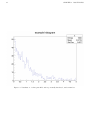
Let’s suppose you want to measure the counts of a Geiger detector located in proximity of a radioactive source in a given
time interval. This would give you an idea of the activity of your source. The count distribution in this case is a Poisson
distribution. Let’s see how operatively you can fill and draw a histogram with the following example macro.
1
2
// Create, Fill and draw an Histogram which reproduces the
// counts of a scaler linked to a Geiger counter.
3
4
5
6
7
8
9
void macro5(){
auto cnt_r_h=new TH1F("count_rate",
"Count Rate;N_{Counts};# occurencies",
100, // Number of Bins
-0.5, // Lower X Boundary
15.5); // Upper X Boundary
10
11
12
13
14
15
auto mean_count=3.6f;
TRandom3 rndgen;
// simulate the measurements
for (int imeas=0;imeas<400;imeas++)
cnt_r_h->Fill(rndgen.Poisson(mean_count));
16
17
18
auto c= new TCanvas();
cnt_r_h->Draw();
19
20
21
auto c_norm= new TCanvas();
cnt_r_h->DrawNormalized();
22
23
24
25
26
27
28
// Print summary
cout << "Moments of Distribution:\n"
<< " - Mean
= " << cnt_r_h->GetMean() << " +- "
<< cnt_r_h->GetMeanError() << "\n"
<< " - Std Dev = " << cnt_r_h->GetStdDev() << " +- "
<< cnt_r_h->GetStdDevError() << "\n"
1 To
optimise the memory usage you might go for one byte (TH1C), short (TH1S), integer (TH1I) or double-precision (TH1D) bin-content.
35
36
CHAPTER 5. HISTOGRAMS
<< " - Skewness = " << cnt_r_h->GetSkewness() << "\n"
<< " - Kurtosis = " << cnt_r_h->GetKurtosis() << "\n";
29
30
31
}
Which gives you the following plot (Figure 5.1):
Figure 5.1: The result of a counting (pseudo) experiment. Only bins corresponding to integer values are filled given the
discrete nature of the poissonian distribution.
Using histograms is rather simple. The main differences with respect to graphs that emerge from the example are:
• line 5 : The histograms have a name and a title right from the start, no predefined number of entries but a number of
bins and a lower-upper range.
• line 15 : An entry is stored in the histogram through the TH1F::Fill method.
• line 18 and 21 : The histogram can be drawn also normalised, ROOT automatically takes cares of the necessary
rescaling.
• line 24 to 30 : This small snippet shows how easy it is to access the moments and associated errors of a histogram.
5.2
Add and Divide Histograms
Quite a large number of operations can be carried out with histograms. The most useful are addition and division. In the
following macro we will learn how to manage these procedures within ROOT.
1
// Divide and add 1D Histograms
2
3
4
5
void format_h(TH1F* h, int linecolor){
h->SetLineWidth(3);
h->SetLineColor(linecolor);
5.2. ADD AND DIVIDE HISTOGRAMS
}
6
7
8
void macro6(){
9
auto
auto
auto
auto
10
11
12
13
sig_h=new TH1F("sig_h","Signal Histo",50,0,10);
gaus_h1=new TH1F("gaus_h1","Gauss Histo 1",30,0,10);
gaus_h2=new TH1F("gaus_h2","Gauss Histo 2",30,0,10);
bkg_h=new TH1F("exp_h","Exponential Histo",50,0,10);
14
// simulate the measurements
TRandom3 rndgen;
for (int imeas=0;imeas<4000;imeas++){
bkg_h->Fill(rndgen.Exp(4));
if (imeas%4==0) gaus_h1->Fill(rndgen.Gaus(5,2));
if (imeas%4==0) gaus_h2->Fill(rndgen.Gaus(5,2));
if (imeas%10==0)sig_h->Fill(rndgen.Gaus(5,.5));}
15
16
17
18
19
20
21
22
// Format Histograms
int i=0;
for (auto hist : {sig_h,bkg_h,gaus_h1,gaus_h2})
format_h(hist,1+i++);
23
24
25
26
27
// Sum
auto sum_h= new TH1F(*bkg_h);
sum_h->Add(sig_h,1.);
sum_h->SetTitle("Exponential + Gaussian;X variable;Y variable");
format_h(sum_h,kBlue);
28
29
30
31
32
33
auto c_sum= new TCanvas();
sum_h->Draw("hist");
bkg_h->Draw("SameHist");
sig_h->Draw("SameHist");
34
35
36
37
38
// Divide
auto dividend=new TH1F(*gaus_h1);
dividend->Divide(gaus_h2);
39
40
41
42
// Graphical Maquillage
dividend->SetTitle(";X axis;Gaus Histo 1 / Gaus Histo 2");
format_h(dividend,kOrange);
gaus_h1->SetTitle(";;Gaus Histo 1 and Gaus Histo 2");
gStyle->SetOptStat(0);
43
44
45
46
47
48
TCanvas* c_divide= new TCanvas();
c_divide->Divide(1,2,0,0);
c_divide->cd(1);
c_divide->GetPad(1)->SetRightMargin(.01);
gaus_h1->DrawNormalized("Hist");
gaus_h2->DrawNormalized("HistSame");
49
50
51
52
53
54
55
56
57
58
59
60
61
}
c_divide->cd(2);
dividend->GetYaxis()->SetRangeUser(0,2.49);
c_divide->GetPad(2)->SetGridy();
c_divide->GetPad(2)->SetRightMargin(.01);
dividend->Draw();
The plots that you will obtain are shown in Figures 5.2 and 5.3.
Some lines now need a bit of clarification:
37
38
CHAPTER 5. HISTOGRAMS
Figure 5.2: The sum of two histograms.
Figure 5.3: The ratio of two histograms.
5.3. TWO-DIMENSIONAL HISTOGRAMS
39
• line 3 : Cling, as we know, is also able to interpret more than one function per file. In this case the function simply
sets up some parameters to conveniently set the line of histograms.
• line 19 to 21 : Some C++ syntax for conditional statements is used to fill the histograms with different numbers of
entries inside the loop.
• line 30 : The sum of two histograms. A weight, which can be negative, can be assigned to the added histogram.
• line 41 : The division of two histograms is rather straightforward.
• line 44 to 62 : When you draw two quantities and their ratios, it is much better if all the information is condensed in
one single plot. These lines provide a skeleton to perform this operation.
5.3
Two-dimensional Histograms
Two-dimensional histograms are a very useful tool, for example to inspect correlations between variables. You can exploit
the bi-dimensional histogram classes provided by ROOT in a simple way. Let’s see how in this macro:
// Draw a Bidimensional Histogram in many ways
// together with its profiles and projections
void macro7(){
gStyle->SetPalette(kBird);
gStyle->SetOptStat(0);
gStyle->SetOptTitle(0);
TH2F bidi_h("bidi_h","2D Histo;Gaussian Vals;Exp. Vals",
30,-5,5, // X axis
30,0,10); // Y axis
TRandom3 rgen;
for (int i=0;i<500000;i++)
bidi_h.Fill(rgen.Gaus(0,2),10-rgen.Exp(4),.1);
auto c=new TCanvas("Canvas","Canvas",800,800);
c->Divide(2,2);
c->cd(1);bidi_h.DrawClone("Cont1");
c->cd(2);bidi_h.DrawClone("Colz");
c->cd(3);bidi_h.DrawClone("lego2");
c->cd(4);bidi_h.DrawClone("surf3");
}
// Profiles and Projections
auto c2=new TCanvas("Canvas2","Canvas2",800,800);
c2->Divide(2,2);
c2->cd(1);bidi_h.ProjectionX()->DrawClone();
c2->cd(2);bidi_h.ProjectionY()->DrawClone();
c2->cd(3);bidi_h.ProfileX()->DrawClone();
c2->cd(4);bidi_h.ProfileY()->DrawClone();
Two kinds of plots are provided within the code, the first one containing three-dimensional representations (Figure 5.4)
and the second one projections and profiles (Figure 5.5) of the bi-dimensional histogram.
When a projection is performed along the x (y) direction, for every bin along the x (y) axis, all bin contents along the y (x)
axis are summed up (upper the plots of Figure 5.5). When a profile is performed along the x (y) direction, for every bin
along the x (y) axis, the average of all the bin contents along the y (x) is calculated together with their RMS and displayed
as a symbol with error bar (lower two plots of Figure 5.5).
Correlations between the variables are quantified by the methods Double_t GetCovariance() and Double_t
GetCorrelationFactor().
40
CHAPTER 5. HISTOGRAMS
Figure 5.4: Different ways of representing bi-dimensional histograms.
5.3. TWO-DIMENSIONAL HISTOGRAMS
Figure 5.5: The projections and profiles of bi-dimensional histograms.
41
42
CHAPTER 5. HISTOGRAMS
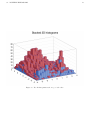
5.4
Multiple histograms
The class THStack allows to manipulate a set of histograms as a single entity. It is a collection of TH1 (or derived) objects.
When drawn, the X and Y axis ranges are automatically computed such as all the histograms will be visible. Several
drawing option are available for both 1D and 2D histograms. The next macros shows how it looks for 2D histograms:
1
// Example of stacked histograms using the class THStack
2
3
4
void hstack(){
THStack *a = new THStack("a","Stacked 2D histograms");
5
TF2 *f1 = new TF2("f1","xygaus + xygaus(5) + xylandau(10)",-4,4,-4,4);
Double_t params1[] = {130,-1.4,1.8,1.5,1, 150,2,0.5,-2,0.5, 3600,-2,0.7,-3,0.3};
f1->SetParameters(params1);
TH2F *h2sta = new TH2F("h2sta","h2sta",20,-4,4,20,-4,4);
h2sta->SetFillColor(38);
h2sta->FillRandom("f1",4000);
6
7
8
9
10
11
12
TF2 *f2 = new TF2("f2","xygaus + xygaus(5)",-4,4,-4,4);
Double_t params2[] = {100,-1.4,1.9,1.1,2, 80,2,0.7,-2,0.5};
f2->SetParameters(params2);
TH2F *h2stb = new TH2F("h2stb","h2stb",20,-4,4,20,-4,4);
h2stb->SetFillColor(46);
h2stb->FillRandom("f2",3000);
13
14
15
16
17
18
19
a->Add(h2sta);
a->Add(h2stb);
20
21
22
23
24
}
a->Draw();
• Line 4 : creates the stack.
• Lines 4-18 : create two histograms to be added in the stack.
• Lines 20-21 : add the histograms in the stack.
• Line 23 : draws the stack as a lego plot. The colour distinguish the two histograms 5.6.
5.4. MULTIPLE HISTOGRAMS
Figure 5.6: Two 2D histograms stack on top of each other.
43
44
CHAPTER 5. HISTOGRAMS
Chapter 6
Functions and Parameter Estimation
After going through the previous chapters, you already know how to use analytical functions (class TF1), and you got some
insight into the graph (TGraphErrors) and histogram classes (TH1F) for data visualisation. In this chapter we will add
more detail to the previous approximate explanations to face the fundamental topic of parameter estimation by fitting
functions to data. For graphs and histograms, ROOT offers an easy-to-use interface to perform fits - either the fit panel of
the graphical interface, or the Fit method. The class TFitResult allows access to the detailed results.
Very often it is necessary to study the statistical properties of analysis procedures. This is most easily achieved by applying
the analysis to many sets of simulated data (or “pseudo data”), each representing one possible version of the true experiment.
If the simulation only deals with the final distributions observed in data, and does not perform a full simulation of the
underlying physics and the experimental apparatus, the name “Toy Monte Carlo” is frequently used.1 Since the true
values of all parameters are known in the pseudo-data, the differences between the parameter estimates from the analysis
procedure w.r.t. the true values can be determined, and it is also possible to check that the analysis procedure provides
correct error estimates.
6.1
Fitting Functions to Pseudo Data
In the example below, a pseudo-data set is produced and a model fitted to it.
ROOT offers various minimisation algorithms to minimise a chi2 or a negative log-likelihood function. The default minimiser
is MINUIT, a package originally implemented in the FORTRAN programming language. A C++ version is also available,
MINUIT2, as well as Fumili (Silin 1983) an algorithm optimised for fitting. The minimisation algorithms can be selected
using the static functions of the ROOT::Math::MinimizerOptions class. Steering options for the minimiser, such as the
convergence tolerance or the maximum number of function calls, can also be set using the methods of this class. All
currently implemented minimisers are documented in the reference documentation of ROOT: have a look for example to
the ROOT::Math::Minimizer class documentation.
1 “Monte Carlo” simulation means that random numbers play a role here which is as crucial as in games of pure chance in the Casino of
Monte Carlo.
45
46
CHAPTER 6. FUNCTIONS AND PARAMETER ESTIMATION
The complication level of the code below is intentionally a little higher than in the previous examples. The graphical
output of the macro is shown in Figure 6.1:
1
2
3
void format_line(TAttLine* line,int col,int sty){
line->SetLineWidth(5); line->SetLineColor(col);
line->SetLineStyle(sty);}
4
5
6
7
double the_gausppar(double* vars, double* pars){
return pars[0]*TMath::Gaus(vars[0],pars[1],pars[2])+
pars[3]+pars[4]*vars[0]+pars[5]*vars[0]*vars[0];}
8
9
10
11
12
int macro8(){
gStyle->SetOptTitle(0); gStyle->SetOptStat(0);
gStyle->SetOptFit(1111); gStyle->SetStatBorderSize(0);
gStyle->SetStatX(.89); gStyle->SetStatY(.89);
13
14
15
TF1 parabola("parabola","[0]+[1]*x+[2]*x**2",0,20);
format_line(&parabola,kBlue,2);
16
17
18
TF1 gaussian("gaussian","[0]*TMath::Gaus(x,[1],[2])",0,20);
format_line(&gaussian,kRed,2);
19
20
21
22
23
24
25
TF1 gausppar("gausppar",the_gausppar,-0,20,6);
double a=15; double b=-1.2; double c=.03;
double norm=4; double mean=7; double sigma=1;
gausppar.SetParameters(norm,mean,sigma,a,b,c);
gausppar.SetParNames("Norm","Mean","Sigma","a","b","c");
format_line(&gausppar,kBlue,1);
26
27
28
TH1F histo("histo","Signal plus background;X vals;Y Vals",50,0,20);
histo.SetMarkerStyle(8);
29
30
31
// Fake the data
for (int i=1;i<=5000;++i) histo.Fill(gausppar.GetRandom());
32
33
34
35
36
37
38
// Reset the parameters before the fit and set
// by eye a peak at 6 with an area of more or less 50
gausppar.SetParameter(0,50);
gausppar.SetParameter(1,6);
int npar=gausppar.GetNpar();
for (int ipar=2;ipar<npar;++ipar) gausppar.SetParameter(ipar,1);
39
40
41
42
43
44
45
46
// perform fit ...
auto fitResPtr = histo.Fit(&gausppar, "S");
// ... and retrieve fit results
fitResPtr->Print(); // print fit results
// get covariance Matrix an print it
TMatrixDSym covMatrix (fitResPtr->GetCovarianceMatrix());
covMatrix.Print();
47
48
49
50
51
52
// Set the values of the gaussian and parabola
for (int ipar=0;ipar<3;ipar++){
gaussian.SetParameter(ipar,gausppar.GetParameter(ipar));
parabola.SetParameter(ipar,gausppar.GetParameter(ipar+3));
}
53
54
55
56
histo.GetYaxis()->SetRangeUser(0,250);
histo.DrawClone("PE");
parabola.DrawClone("Same"); gaussian.DrawClone("Same");
6.2. TOY MONTE CARLO EXPERIMENTS
TLatex latex(2,220,"#splitline{Signal Peak over}{background}");
latex.DrawClone("Same");
return 0;
57
58
59
60
47
}
Some step by step explanation is at this point necessary:
• Lines 1-3 : A simple function to ease the make-up of lines. Remember that the class TF1 inherits from TAttLine.
• Lines 5-7 : Definition of a customised function, namely a Gaussian (the “signal”) plus a parabolic function, the
“background”.
• Lines 10-12 : Some make-up for the Canvas. In particular we want that the parameters of the fit appear very clearly
and nicely on the plot.
• Lines 20-25 : Define and initialise an instance of TF1.
• Lines 27-31 : Define and fill a histogram.
• Lines 33-38 : For convenience, the same function as for the generation of the pseudo-data is used in the fit; hence, we
need to reset the function parameters. This part of the code is very important for each fit procedure, as it sets the
initial values of the fit.
• Line 41 : A very simple command, well known by now: fit the function to the histogram.
• Lines 42-46 : Retrieve the output from the fit. Here, we simply print the fit result and access and print the covariance
matrix of the parameters.
• Lines 54-end: Plot the pseudo-data, the fitted function and the signal and background components at the best-fit
values.
6.2
Toy Monte Carlo Experiments
Let us look at a simple example of a toy experiment comparing two methods to fit a function to a histogram, the χ2
method and a method called “binned log-likelihood fit”, both available in ROOT.
As a very simple yet powerful quantity to check the quality of the fit results, we construct for each pseudo-data set the
so-called “pull”, the difference of the estimated and the true value of a parameter, normalised to the estimated error on the
true )
parameter, (pestimσ−p
. If everything is OK, the distribution of the pull values is a standard normal distribution, i.e. a
p
Gaussian distribution centred around zero with a standard deviation of one.
The macro performs a rather big number of toy experiments, where a histogram is repeatedly filled with Gaussian distributed
numbers, representing the pseudo-data in this example. Each time, a fit is performed according to the selected method,
and the pull is calculated and filled into a histogram. Here is the code:
1
2
3
// Toy Monte Carlo example.
// Check pull distribution to compare chi2 and binned
// log-likelihood methods.
4
5
6
7
8
void pull( int n_toys = 10000,
int n_tot_entries = 100,
int nbins = 40,
bool do_chi2=true ){
9
10
11
12
TString method_prefix("Log-Likelihood ");
if (do_chi2)
method_prefix="#chi^{2} ";
13
14
// Create histo
48
CHAPTER 6. FUNCTIONS AND PARAMETER ESTIMATION
Figure 6.1: Fit of pseudo data: a signal shape over a background trend. This plot is another example of how making a plot
“self-explanatory” can help you better displaying your results.
6.2. TOY MONTE CARLO EXPERIMENTS
TH1F h4(method_prefix+"h4",
method_prefix+" Random Gauss",
nbins,-4,4);
h4.SetMarkerStyle(21);
h4.SetMarkerSize(0.8);
h4.SetMarkerColor(kRed);
15
16
17
18
19
20
21
// Histogram for sigma and pull
TH1F sigma(method_prefix+"sigma",
method_prefix+"sigma from gaus fit",
50,0.5,1.5);
TH1F pull(method_prefix+"pull",
method_prefix+"pull from gaus fit",
50,-4.,4.);
22
23
24
25
26
27
28
29
// Make nice canvases
auto c0 = new TCanvas(method_prefix+"Gauss",
method_prefix+"Gauss",0,0,320,240);
c0->SetGrid();
30
31
32
33
34
// Make nice canvases
auto c1 = new TCanvas(method_prefix+"Result",
method_prefix+"Sigma-Distribution",
0,300,600,400);
c0->cd();
35
36
37
38
39
40
float sig, mean;
for (int i=0; i<n_toys; i++){
// Reset histo contents
h4.Reset();
// Fill histo
for ( int j = 0; j<n_tot_entries; j++ )
h4.Fill(gRandom->Gaus());
// perform fit
if (do_chi2) h4.Fit("gaus","q"); // Chi2 fit
else h4.Fit("gaus","lq"); // Likelihood fit
// some control output on the way
if (!(i%100)){
h4.Draw("ep");
c0->Update();}
41
42
43
44
45
46
47
48
49
50
51
52
53
54
55
56
57
58
59
60
61
62
63
64
65
66
}
// Get sigma from fit
TF1 *fit = h4.GetFunction("gaus");
sig = fit->GetParameter(2);
mean= fit->GetParameter(1);
sigma.Fill(sig);
pull.Fill(mean/sig * sqrt(n_tot_entries));
} // end of toy MC loop
// print result
c1->cd();
pull.DrawClone();
67
68
69
70
71
72
73
void macro9(){
int n_toys=10000;
int n_tot_entries=100;
int n_bins=40;
cout << "Performing Pull Experiment with chi2 \n";
pull(n_toys,n_tot_entries,n_bins,true);
49
50
74
75
76
}
CHAPTER 6. FUNCTIONS AND PARAMETER ESTIMATION
cout << "Performing Pull Experiment with Log Likelihood\n";
pull(n_toys,n_tot_entries,n_bins,false);
Your present knowledge of ROOT should be enough to understand all the technicalities behind the macro. Note that the
variable pull in line 61 is different from the definition above: instead of the parameter error on mean, the fitted standard
deviation of the distribution divided by the square root of the number of entries, sig/sqrt(n_tot_entries), is used.
• What method exhibits the better performance with the default parameters ?
• What happens if you increase the number of entries per histogram by a factor of ten ? Why ?
The answers to these questions are well beyond the scope of this guide. Basically all books about statistical methods
provide a complete treatment of the aforementioned topics.
Chapter 7
File I/O and Parallel Analysis
7.1
Storing ROOT Objects
ROOT offers the possibility to write instances of classes on disk, into a ROOT-file (see the TFile class for more details).
One says that the object is made “persistent” by storing it on disk. When reading the file back, the object is reconstructed
in memory. The requirement to be satisfied to perform I/O of instances of a certain class is that the ROOT type system is
aware of the layout in memory of that class. This topic is beyond the scope of this document: it is worth to mention that
I/O can be performed out of the box for the almost complete set of ROOT classes.
We can explore this functionality with histograms and two simple macros.
void write_to_file(){
// Instance of our histogram
TH1F h("my_histogram","My Title;X;# of entries",100,-5,5);
// Let's fill it randomly
h.FillRandom("gaus");
// Let's open a TFile
TFile out_file("my_rootfile.root","RECREATE");
// Write the histogram in the file
h.Write();
}
// Close the file
out_file.Close();
Not bad, eh ? Especially for a language that does not foresees persistency natively like C++. The RECREATE option
forces ROOT to create a new file even if a file with the same name exists on disk.
Now, you may use the Cling command line to access information in the file and draw the previously written histogram:
> root my_rootfile.root
root [0]
Attaching file my_rootfile.root as _file0...
root [1] _file0->ls()
TFile**
my_rootfile.root
TFile*
my_rootfile.root
KEY: TH1F my_histogram;1 My Title
root [2] my_histogram->Draw()
51
52
CHAPTER 7. FILE I/O AND PARALLEL ANALYSIS
Alternatively, you can use a simple macro to carry out the job:
void read_from_file(){
// Let's open the TFile
TFile in_file("my_rootfile.root");
// Get the Histogram out
TH1F* h;
in_file.GetObject("my_histogram",h);
// Draw it
h->Draw();
}
7.2
N-tuples in ROOT
7.2.1
Storing simple N-tuples
Up to now we have seen how to manipulate input read from ASCII files. ROOT offers the possibility to do much better
than that, with its own n-tuple classes. Among the many advantages provided by these classes one could cite
• Optimised disk I/O.
• Possibility to store many n-tuple rows.
• Write the n-tuples in ROOT files.
• Interactive inspection with TBrowser.
• Store not only numbers, but also objects in the columns.
In this section we will discuss briefly the TNtuple class, which is a simplified version of the TTree class. A ROOT TNtuple
object can store rows of float entries. Let’s tackle the problem according to the usual strategy commenting a minimal
example
// Fill an n-tuple and write it to a file simulating measurement of
// conductivity of a material in different conditions of pressure
// and temperature.
void write_ntuple_to_file(){
TFile ofile("conductivity_experiment.root","RECREATE");
// Initialise the TNtuple
TNtuple cond_data("cond_data",
"Example N-Tuple",
"Potential:Current:Temperature:Pressure");
// Fill it randomly to fake the acquired data
TRandom3 rndm;
float pot,cur,temp,pres;
for (int i=0;i<10000;++i){
pot=rndm.Uniform(0.,10.);
// get voltage
temp=rndm.Uniform(250.,350.); // get temperature
pres=rndm.Uniform(0.5,1.5);
// get pressure
cur=pot/(10.+0.05*(temp-300.)-0.2*(pres-1.)); // current
// add some random smearing (measurement errors)
53
7.2. N-TUPLES IN ROOT
pot*=rndm.Gaus(1.,0.01); // 1% error
temp+=rndm.Gaus(0.,0.3); // 0.3 abs.
pres*=rndm.Gaus(1.,0.02);// 1% error
cur*=rndm.Gaus(1.,0.01); // 1% error
// write to ntuple
cond_data.Fill(pot,cur,temp,pres);
}
}
on voltage
error on temp.
on pressure
on current
// Save the ntuple and close the file
cond_data.Write();
ofile.Close();
This data written to this example n-tuple represents, in the statistical sense, three independent variables (Potential or
Voltage, Pressure and Temperature), and one variable (Current) which depends on the others according to very simple
laws, and an additional Gaussian smearing. This set of variables mimics a measurement of an electrical resistance while
varying pressure and temperature.
Imagine your task now consists in finding the relations among the variables – of course without knowing the code used to
generate them. You will see that the possibilities of the NTuple class enable you to perform this analysis task. Open the
ROOT file (cond_data.root) written by the macro above in an interactive session and use a TBrowser to interactively
inspect it:
root[0] TBrowser b
You find the columns of your n-tuple written as leafs. Simply clicking on them you can obtain histograms of the variables!
Next, try the following commands at the shell prompt and in the interactive ROOT shell, respectively:
> root conductivity_experiment.root
Attaching file conductivity_experiment.root as _file0...
root [0] cond_data->Draw("Current:Potential")
You just produced a correlation plot with one single line of code!
Try to extend the syntax typing for example
root [1] cond_data->Draw("Current:Potential","Temperature<270")
What do you obtain ?
Now try
root [2] cond_data->Draw("Current/Potential:Temperature")
It should have become clear from these examples how to navigate in such a multi-dimensional space of variables and unveil
relations between variables using n-tuples.
7.2.2
Reading N-tuples
For completeness, you find here a small macro to read the data back from a ROOT n-tuple
// Read the previously produced N-Tuple and print on screen
// its content
void read_ntuple_from_file(){
// Open a file, save the ntuple and close the file
54
CHAPTER 7. FILE I/O AND PARALLEL ANALYSIS
TFile in_file("conductivity_experiment.root");
TNtuple* my_tuple;in_file.GetObject("cond_data",my_tuple);
float pot,cur,temp,pres; float* row_content;
cout << "Potential\tCurrent\tTemperature\tPressure\n";
for (int irow=0;irow<my_tuple->GetEntries();++irow){
my_tuple->GetEntry(irow);
row_content = my_tuple->GetArgs();
pot = row_content[0];
cur = row_content[1];
temp = row_content[2];
pres = row_content[3];
cout << pot << "\t" << cur << "\t" << temp
<< "\t" << pres << endl;
}
}
The macro shows the easiest way of accessing the content of a n-tuple: after loading the n-tuple, its branches are assigned
to variables and GetEntry(long) automatically fills them with the content for a specific row. By doing so, the logic for
reading the n-tuple and the code to process it can be split and the source code remains clear.
7.2.3
Storing Arbitrary N-tuples
It is also possible to write n-tuples of arbitrary type by using ROOT’s TBranch class. This is especially important as
TNtuple::Fill() accepts only floats. The following macro creates the same n-tuple as before but the branches are booked
directly. The Fill() function then fills the current values of the connected variables to the tree.
// Fill an n-tuple and write it to a file simulating measurement of
// conductivity of a material in different conditions of pressure
// and temperature using branches.
void write_ntuple_to_file_advanced(
const std::string& outputFileName="conductivity_experiment.root"
,unsigned int numDataPoints=1000000){
TFile ofile(outputFileName.c_str(),"RECREATE");
// Initialise the TNtuple
TTree cond_data("cond_data", "Example N-Tuple");
// define the variables and book them for the ntuple
float pot,cur,temp,pres;
cond_data.Branch("Potential", &pot, "Potential/F");
cond_data.Branch("Current", &cur, "Current/F");
cond_data.Branch("Temperature", &temp, "Temperature/F");
cond_data.Branch("Pressure", &pres, "Pressure/F");
for (int i=0;i<numDataPoints;++i){
// Fill it randomly to fake the acquired data
pot=gRandom->Uniform(0.,10.)*gRandom->Gaus(1.,0.01);
temp=gRandom->Uniform(250.,350.)+gRandom->Gaus(0.,0.3);
pres=gRandom->Uniform(0.5,1.5)*gRandom->Gaus(1.,0.02);
cur=pot/(10.+0.05*(temp-300.)-0.2*(pres-1.))*
gRandom->Gaus(1.,0.01);
// write to ntuple
cond_data.Fill();}
55
7.2. N-TUPLES IN ROOT
}
// Save the ntuple and close the file
cond_data.Write();
ofile.Close();
The Branch() function requires a pointer to a variable and a definition of the variable type. The following table lists
some of the possible values. Please note that ROOT is not checking the input and mistakes are likely to result in serious
problems. This holds especially if values are read as another type than they have been written, e.g. when storing a variable
as float and reading it as double.
List of variable types that can be used to define the type of a branch in ROOT:
type
size
C++
identifier
signed integer
32 bit
int
I
64 bit
long
L
32 bit
unsigned int
i
64 bit
unsigned long
l
32 bit
float
F
64 bit
double
D
-
bool
O
unsigned integer
floating point
boolean
7.2.4
Processing N-tuples Spanning over Several Files
Usually n-tuples or trees span over many files and it would be difficult to add them manually. ROOT thus kindly provides
a helper class in the form of TChain. Its usage is shown in the following macro which is very similar to the previous
example. The constructor of a TChain takes the name of the TTree (or TNuple) as an argument. The files are added with
the function Add(fileName), where one can also use wild-cards as shown in the example.
//
//
//
//
//
//
//
//
//
//
Read several previously produced N-Tuples and print on screen its
content.
you can easily create some files with the following statement:
for i in 0 1 2 3 4 5; \\
do root -l -x -b -q \\
"write_ntuple_to_file.cxx \\
(\"conductivity_experiment_${i}.root\", 100)"; \\
done
void read_ntuple_with_chain(){
// initiate a TChain with the name of the TTree to be processed
TChain in_chain("cond_data");
in_chain.Add("conductivity_experiment*.root"); // add files,
// wildcards work
// define variables and assign them to the corresponding branches
float pot, cur, temp, pres;
in_chain.SetBranchAddress("Potential", &pot);
in_chain.SetBranchAddress("Current", &cur);
in_chain.SetBranchAddress("Temperature", &temp);
in_chain.SetBranchAddress("Pressure", &pres);
cout << "Potential\tCurrent\tTemperature\tPressure\n";
for (size_t irow=0; irow<in_chain.GetEntries(); ++irow){
56
}
CHAPTER 7. FILE I/O AND PARALLEL ANALYSIS
}
7.2.5
in_chain.GetEntry(irow); // loads all variables that have
// been connected to branches
cout << pot << "\t" << cur << "\t" << temp <<
"\t" << pres << endl;
For the advanced user: Processing trees with a selector script
Another very general and powerful way of processing a TChain is provided via the method TChain::Process(). This
method takes as arguments an instance of a – user-implemented– class of type TSelector, and – optionally – the
number of entries and the first entry to be processed. A template for the class TSelector is provided by the method
TTree::MakeSelector, as is shown in the little macro makeSelector.C below.
It opens the n-tuple conductivity_experiment.root from the example above and creates from it the header file
MySelector.h and a template to insert your own analysis code, MySelector.C.
7.2. N-TUPLES IN ROOT
57
{
// create template class for Selector to run on a tree
//////////////////////////////////////////////////////
//
// open root file containing the Tree
TFile f("conductivity_experiment.root");
// create TTree object from it
TTree *t; f.GetObject("cond_data",t);
// this generates the files MySelector.h and MySelector.C
t->MakeSelector("MySelector");
}
The template contains the entry points Begin() and SlaveBegin() called before processing of the TChain starts, Process()
called for every entry of the chain, and SlaveTerminate() and Terminate() called after the last entry has been processed.
Typically, initialization like booking of histograms is performed in SlaveBegin(), the analysis, i.e. the selection of entries,
calculations and filling of histograms, is done in Process(), and final operations like plotting and storing of results happen
in SlaveTerminate() or Terminate().
The entry points SlaveBegin() and SlaveTerminate() are called on so-called slave nodes only if parallel processing via
PROOF or PROOF lite is enabled, as will be explained below.
A simple example of a selector class is shown in the macro MySelector.C. The example is executed with the following
sequence of commands:
> TChain *ch=new TChain("cond_data", "Chain for Example N-Tuple");
> ch->Add("conductivity_experiment*.root");
> ch->Process("MySelector.C+");
As usual, the “+” appended to the name of the macro to be executed initiates the compilation of the MySelector.C with
the system compiler in order to improve performance.
The code in MySelector.C, shown in the listing below, books some histograms in SlaveBegin() and adds them to the
instance fOutput, which is of the class TList.1 The final processing in Terminate() allows to access histograms and store,
display or save them as pictures. This is shown in the example via the TList fOutput. See the commented listing below
for more details; most of the text is actually comments generated automatically by TTree::MakeSelector.
#define MySelector_cxx
// The class definition in MySelector.h has been generated automatically
// by the ROOT utility TTree::MakeSelector(). This class is derived
// from the ROOT class TSelector. For more information on the TSelector
// framework see $ROOTSYS/README/README.SELECTOR or the ROOT User Manual.
// The following methods are defined in this file:
//
Begin():
called every time a loop on the tree starts,
//
a convenient place to create your histograms.
//
SlaveBegin():
called after Begin(), when on PROOF called only on the
//
slave servers.
//
Process():
called for each event, in this function you decide what
//
to read and fill your histograms.
//
SlaveTerminate: called at the end of the loop on the tree, when on PROOF
//
called only on the slave servers.
//
Terminate():
called at the end of the loop on the tree,
//
a convenient place to draw/fit your histograms.
//
// To use this file, try the following session on your Tree T:
//
// root> T->Process("MySelector.C")
1 The usage of fOutput is not really needed for this simple example, but it allows re-usage of the exact code in parallel processing with PROOF
(see next section).
58
CHAPTER 7. FILE I/O AND PARALLEL ANALYSIS
// root> T->Process("MySelector.C","some options")
// root> T->Process("MySelector.C+")
//
#include "MySelector.h"
#include <TH2.h>
#include <TStyle.h>
void MySelector::Begin(TTree * /*tree*/ )
{
// The Begin() function is called at the start of the query.
// When running with PROOF Begin() is only called on the client.
// The tree argument is deprecated (on PROOF 0 is passed).
TString option = GetOption();
}
void MySelector::SlaveBegin(TTree * /*tree*/ )
{
// The SlaveBegin() function is called after the Begin() function.
// When running with PROOF SlaveBegin() is called on each slave server.
// The tree argument is deprecated (on PROOF 0 is passed).
TString option = GetOption();
}
Bool_t MySelector::Process(Long64_t entry)
{
// The Process() function is called for each entry in the tree (or possibly
// keyed object in the case of PROOF) to be processed. The entry argument
// specifies which entry in the currently loaded tree is to be processed.
// It can be passed to either MySelector::GetEntry() or TBranch::GetEntry()
// to read either all or the required parts of the data. When processing
// keyed objects with PROOF, the object is already loaded and is available
// via the fObject pointer.
//
// This function should contain the "body" of the analysis. It can contain
// simple or elaborate selection criteria, run algorithms on the data
// of the event and typically fill histograms.
//
// The processing can be stopped by calling Abort().
//
// Use fStatus to set the return value of TTree::Process().
//
// The return value is currently not used.
}
return kTRUE;
void MySelector::SlaveTerminate()
{
// The SlaveTerminate() function is called after all entries or objects
// have been processed. When running with PROOF SlaveTerminate() is called
// on each slave server.
}
7.2. N-TUPLES IN ROOT
59
void MySelector::Terminate()
{
// The Terminate() function is the last function to be called during
// a query. It always runs on the client, it can be used to present
// the results graphically or save the results to file.
}
7.2.6
For power-users: Multi-core processing with PROOF lite
The processing of n-tuples via a selector function of type TSelector through TChain::Process(), as described at the end
of the previous section, offers an additional advantage in particular for very large data sets: on distributed systems or
multi-core architectures, portions of data can be processed in parallel, thus significantly reducing the execution time. On
modern computers with multi-core CPUs or hardware-threading enabled, this allows a much faster turnaround of analyses,
since all the available CPU power is used.
On distributed systems, a PROOF server and worker nodes have to be set up, as described in detail in the ROOT
documentation. On a single computer with multiple cores, PROOF lite can be used instead. Try the following little macro,
RunMySelector.C, which contains two extra lines compared to the example above (adjust the number of workers according
to the number of CPU cores):
{// set up a TChain
TChain *ch=new TChain("cond_data", "My Chain for Example N-Tuple");
ch->Add("conductivity_experiment*.root");
// eventually, start Proof Lite on cores
TProof::Open("workers=4");
ch->SetProof();
ch->Process("MySelector.C+");}
The first command, TProof::Open(const char*) starts a local PROOF server (if no arguments are specified, all cores
will be used), and the command ch->SetProof(); enables processing of the chain using PROOF. Now, when issuing the
command ch->Process("MySelector.C+);, the code in MySelector.C is compiled and executed on each slave node. The
methods Begin() and Terminate() are executed on the master only. The list of n-tuple files is analysed, and portions
of the data are assigned to the available slave processes. Histograms booked in SlaveBegin() exist in the processes on
the slave nodes, and are filled accordingly. Upon termination, the PROOF master collects the histograms from the slaves
and merges them. In Terminate() all merged histograms are available and can be inspected, analysed or stored. The
histograms are handled via the instances fOutput of class TList in each slave process, and can be retrieved from this list
after merging in Terminate.
To explore the power of this mechanism, generate some very large n-tuples using the script from the section Storing Arbitrary
N-tuples - you could try 10 000 000 events (this results in a large n-tuple of about 160 MByte in size). You could also
generate a large number of files and use wildcards to add the to the TChain. Now execute: > root -l RunMySelector.C
and watch what happens:
Processing RunMySelector.C...
+++ Starting PROOF-Lite with 4 workers +++
Opening connections to workers: OK (4 workers)
Setting up worker servers: OK (4 workers)
PROOF set to parallel mode (4 workers)
Info in <TProofLite::SetQueryRunning>: starting query: 1
Info in <TProofQueryResult::SetRunning>: nwrks: 4
Info in <TUnixSystem::ACLiC>: creating shared library
~/DivingROOT/macros/MySelector_C.so
*==* ----- Begin of Job ----- Date/Time = Wed Feb 15 23:00:04 2012
Looking up for exact location of files: OK (4 files)
Looking up for exact location of files: OK (4 files)
60
CHAPTER 7. FILE I/O AND PARALLEL ANALYSIS
Info in <TPacketizerAdaptive::TPacketizerAdaptive>:
Setting max number of workers per node to 4
Validating files: OK (4 files)
Info in <TPacketizerAdaptive::InitStats>:
fraction of remote files 1.000000
Info in <TCanvas::Print>:
file ResistanceDistribution.png has been created
*==* ----- End of Job ----- Date/Time = Wed Feb 15 23:00:08 2012
Lite-0: all output objects have been merged
Log files of the whole processing chain are kept in the directory ~.proof for each worker node. This is very helpful for
debugging or if something goes wrong. As the method described here also works without using PROOF, the development
work on an analysis script can be done in the standard way on a small subset of the data, and only for the full processing
one would use parallelism via PROOF.
It is worth to remind the reader that the speed of typical data analysis programs limited by the I/O speed (for example
the latencies implied by reading data from a hard drive). It is therefore expected that this limitation cannot be eliminated
with the usage of any parallel analysis toolkit.
7.2.7
Optimisation Regarding N-tuples
ROOT automatically applies compression algorithms on n-tuples to reduce the memory consumption. A value that is in
most cases the same will consume only small space on your disk (but it has to be decompressed on reading). Nevertheless,
you should think about the design of your n-tuples and your analyses as soon as the processing time exceeds some minutes.
• Try to keep your n-tuples simple and use appropriate variable types. If your measurement has only a limited precision,
it is needless to store it with double precision.
• Experimental conditions that do not change with every single measurement should be stored in a separate tree.
Although the compression can handle redundant values, the processing time increase with every variable that has to
be filled.
• The function SetCacheSize(long) specifies the size of the cache for reading a TTree object from a file. The default
value is 30MB. A manual increase may help in certain situations. Please note that the caching mechanism can cover
only one TTree object per TFile object.
• You can select the branches to be covered by the caching algorithm with AddBranchToCache and deactivate unneeded
branches with SetBranchStatus. This mechanism can result in a significant speed-up for simple operations on trees
with many branches.
• You can measure the performance easily with TTreePerfStats. The ROOT documentation on this class also includes
an introductory example. For example, TTreePerfStats can show you that it is beneficial to store meta data and
payload data separately, i.e. write the meta data tree in a bulk to a file at the end of your job instead of writing both
trees interleaved.
Chapter 8
ROOT in Python
ROOT offers the possibility to interface to Python via a set of bindings called PyROOT. Python is used in a wide variety
of application areas and one of the most used scripting languages today. With the help of PyROOT it becomes possible to
combine the power of a scripting language with ROOT tools. Introductory material to Python is available from many
sources on the web, see e. g. http://docs.python.org.
8.1
PyROOT
The access to ROOT classes and their methods in PyROOT is almost identical to C++ macros, except for the special
language features of Python, most importantly dynamic type declaration at the time of assignment. Coming back to our
first example, simply plotting a function in ROOT, the following C++ code:
TF1 *f1 = new TF1("f2","[0]*sin([1]*x)/x",0.,10.);
f1->SetParameter(0,1);
f1->SetParameter(1,1);
f1->Draw();
in Python becomes:
import ROOT
f1 = ROOT.TF1("f2","[0]*sin([1]*x)/x",0.,10.)
f1.SetParameter(0,1);
f1.SetParameter(1,1);
f1.Draw();
A slightly more advanced example hands over data defined in the macro to the ROOT class TGraphErrors. Note that a
Python array can be used to pass data between Python and ROOT. The first line in the Python script allows it to be
executed directly from the operating system, without the need to start the script from python or the highly recommended
powerful interactive shell ipython. The last line in the python script is there to allow you to have a look at the graphical
output in the ROOT canvas before it disappears upon termination of the script.
Here is the C++ version:
void TGraphFit(){
//
// Draw a graph with error bars and fit a function to it
//
gStyle->SetOptFit(111) ; //superimpose fit results
// make nice Canvas
TCanvas *c1 = new TCanvas("c1" ,"Daten" ,200 ,10 ,700 ,500) ;
c1->SetGrid( ) ;
61
62
}
CHAPTER 8. ROOT IN PYTHON
//define some data points ...
const Int_t n = 10;
Float_t x[n] = {-0.22, 0.1, 0.25, 0.35, 0.5, 0.61, 0.7, 0.85, 0.89, 1.1};
Float_t y[n] = {0.7, 2.9, 5.6, 7.4, 9., 9.6, 8.7, 6.3, 4.5, 1.1};
Float_t ey[n] = {.8 ,.7 ,.6 ,.5 ,.4 ,.4 ,.5 ,.6 ,.7 ,.8};
Float_t ex[n] = {.05 ,.1 ,.07 ,.07 ,.04 ,.05 ,.06 ,.07 ,.08 ,.05};
// and hand over to TGraphErros object
TGraphErrors *gr = new TGraphErrors(n,x,y,ex,ey);
gr->SetTitle("TGraphErrors with Fit") ;
gr->Draw("AP");
// now perform a fit (with errors in x and y!)
gr->Fit("gaus");
c1->Update();
In Python it looks like this:
#
# Draw a graph with error bars and fit a function to it
#
from ROOT import gStyle, TCanvas, TGraphErrors
from array import array
gStyle.SetOptFit (111) # superimpose fit results
c1=TCanvas("c1" ,"Data" ,200 ,10 ,700 ,500) #make nice
c1.SetGrid ()
#define some data points . . .
x = array('f', (-0.22, 0.1, 0.25, 0.35, 0.5, 0.61, 0.7, 0.85, 0.89, 1.1) )
y = array('f', (0.7, 2.9, 5.6, 7.4, 9., 9.6, 8.7, 6.3, 4.5, 1.1) )
ey = array('f', (.8 ,.7 ,.6 ,.5 ,.4 ,.4 ,.5 ,.6 ,.7 ,.8) )
ex = array('f', (.05 ,.1 ,.07 ,.07 ,.04 ,.05 ,.06 ,.07 ,.08 ,.05) )
nPoints=len ( x )
# . . . and hand over to TGraphErros object
gr=TGraphErrors ( nPoints , x , y , ex , ey )
gr.SetTitle("TGraphErrors with Fit")
gr.Draw ( "AP" ) ;
gr.Fit("gaus")
c1.Update ()
# request user action before ending (and deleting graphics window)
raw_input('Press <ret> to end -> ')
Comparing the C++ and Python versions in these two examples, it now should be clear how easy it is to convert any
ROOT Macro in C++ to a Python version.
As another example, let us revisit macro3 from Chapter 4. A straight-forward Python version relying on the ROOT class
TMath:
# Builds a polar graph in a square Canvas.
from ROOT import TGraphPolar, TCanvas, TMath
from array import array
c = TCanvas("myCanvas","myCanvas",600,600)
rmin = 0.
rmax = TMath.Pi()*6.
npoints = 300
r = array('d',[0]*npoints)
theta = array('d',[0]*npoints)
for ipt in xrange(0,npoints):
r[ipt] = ipt*(rmax-rmin)/npoints+rmin
8.2. CUSTOM CODE: FROM C++ TO PYTHON
63
theta[ipt] = TMath.Sin(r[ipt])
grP1 = TGraphPolar(npoints,r,theta)
grP1.SetTitle("A Fan")
grP1.SetLineWidth(3)
grP1.SetLineColor(2)
grP1.DrawClone("L")
raw_input("Press enter to exit.")
8.1.1
More Python- less C++
You may have noticed already that there are some Python modules providing functionality similar to ROOT classes, which
fit more seamlessly into your Python code.
A more “pythonic” version of the above macro3 would use a replacement of the ROOT class TMath for the provisoining of
data to TGraphPolar. With the math package, the part of the code becomes
import math
from array import array
from ROOT import TCanvas , TGraphPolar
...
ipt=range(0,npoints)
r=array('d',map(lambda x: x*(rmax-rmin)/(npoints-1.)+rmin,ipt))
theta=array('d',map(math.sin,r))
e=array('d',npoints*[0.])
...
8.1.1.1
Customised Binning
This example combines comfortable handling of arrays in Python to define variable bin sizes of a ROOT histogram. All we
need to know is the interface of the relevant ROOT class and its methods (from the ROOT documentation):
TH1F(const char* name , const char* title , Int_t nbinsx , const Double_t* xbins)
Here is the Python code:
import ROOT
from array import array
arrBins = array('d' ,(1 ,4 ,9 ,16) ) # array of bin edges
histo = ROOT.TH1F("hist", "hist", len(arrBins)-1, arrBins)
# fill it with equally spaced numbers
for i in range (1 ,16) :
histo.Fill(i)
histo.Draw ()
8.2
Custom code: from C++ to Python
The ROOT interpreter and type sytem offer interesting possibilities when it comes to JITting of C++ code. Take for
example this header file, containing a class and a function.
// file cpp2pythonExample.h
#include "stdio.h"
class A{
public:
64
CHAPTER 8. ROOT IN PYTHON
A(int i):m_i(i){}
int getI() const {return m_i;}
private:
int m_i=0;
};
void printA(const A& a ){
printf ("The value of A instance is %i.\n",a.getI());
}
>>>
>>>
>>>
>>>
The
import ROOT
ROOT.gInterpreter.ProcessLine('#include "cpp2pythonExample.h"')
a = ROOT.A(123)
ROOT.printA(a)
value of A instance is 123.
This example might seem trivial, but it shows a powerful ROOT feature. C++ code can be JITted within PyROOT and
the entities defined in C++ can be transparently used in Python!
Chapter 9
Concluding Remarks
This is the end of our guided tour for beginners through ROOT. There is still a lot coming to mind to be said, but by now
you are experienced enough to use the ROOT documentation, most importantly the ROOT home page and the ROOT
reference guide with the documentation of all ROOT classes, or the ROOT users guide.
A very useful way for you to continue exploring ROOT is to study the examples in the sub-directory tutorials/ of any
ROOT installation.
There are some powerful features of ROOT which were not treated in this document, e.g. packages named RooFit and
RooStats providing an advanced framework for model building, fitting and statistical analysis. The ROOT namespace TMVA
offers multi-variate analysis tools including an artificial neural network and many other advanced tools for classification
problems. The remarkable ability of ROOT to handle large data volumes was already mentioned in this guide, implemented
through the class TTree. But there is still much more for you to explore!
End of this guide . . . but hopefully not of your interaction with ROOT !
65
66
CHAPTER 9. CONCLUDING REMARKS
Chapter 10
References
Matsumoto, Makoto. 1997. “Mersenne Twister Home Page.” http://www.math.sci.hiroshima-u.ac.jp/~m-mat/MT/emt.
html.
Silin, I.N. 1983. “FUMILI.” CERN Program Library d510.
The ROOT Reference Guide. 2013. http://root.cern.ch/drupal/content/reference-guide.
The ROOT Users Guide. 2015. http://root.cern.ch/drupal/content/users-guide.
“What Is Cling.” 2015. https://root.cern.ch/drupal/content/cling.
67