Download A ROOT Guide For Students

Institut für Experimentelle Kernphysik
A ROOT Guide For Students
“Diving Into ROOT”
http://root.cern.ch
Abstract:
ROOT is an object-oriented framework for data analysis. Among its prominent features are an advanced
graphical user interface for visualization and interactive data analysis and an interpreter for the C++
programming language, which allows rapid prototyping of analysis code based on the C++ classes provided by ROOT. Access to ROOT classes is also possible from the very versatile and popular scripting
language Python.
This introductory guide shows the main features applicable to typical problems of data analysis in student labs: input and plotting of data from measurements and comparison with and fitting of analytical
functions. Although appearing to be quite a heavy
gun for some of the simpler problems, getting used to
a tool like ROOT at this stage is an optimal preparation for the demanding tasks in state-of-the art,
scientific data analysis.
Authors:
Danilo Piparo,
Günter Quast,
Manuel Zeise
Version of December 5, 2013
CHAPTER
1
MOTIVATION AND INTRODUCTION
Welcome to data analysis !
Comparison of measurements to theoretical models is one of the standard tasks in experimental physics.
In the most simple case, a “model” is just a function providing predictions of measured data. Very often,
the model depends on parameters. Such a model may simply state “the current I is proportional to the
voltage U ”, and the task of the experimentalist consists of determining the resistance, R, from a set of
measurements.
As a first step, a visualisation of the data is needed. Next, some manipulations typically have to be
applied, e. g. corrections or parameter transformations. Quite often, these manipulations are complex
ones, and a powerful library of mathematical functions and procedures should be provided - think for
example of an integral or peak-search or a Fourier transformation applied to an input spectrum to obtain
the actual measurement described by the model.
One specialty of experimental physics are the inevitable errors affecting each measurement, and visualization tools have to include these. In subsequent analysis, the statistical nature of the errors must be
handled properly.
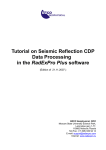
As the last step, measurements are compared to models, and free model parameters need to be determined in this process , see Figure1.1 for an example of a function (model) fit to data points. Several
standard methods are available, and a data analysis tool should provide easy access to more than one of
them. Means to quantify the level of agreement between measurements and model must also be available.
1
0.9
0.8
Y = f (x)
0.7
0.6
0.5
0.4
Data
0.3
Model
0.2
0
1
2
3
4
Fi
oo
R
b
La
X
Figure 1.1.: Measured data points with error bars and fitted quadratic function .
3
1. Motivation and Introduction
Quite often, the data volume to be analyzed is large - think of fine-granular measurements accumulated
with the aid of computers. A usable tool therefore must contain easy-to-use and efficient methods for
data handling.
In Quantum mechanics, models typically only predict the probability density function (“pdf”) of measurements depending on a number of parameters, and the aim of the experimental analysis is to extract
the parameters from the observed distribution of frequencies at which certain values of the measurement
are observed. Measurements of this kind require means to generate and visualize frequency distributions,
so-called histograms, and stringent statistical treatment to extract the model parameters from purely
statistical distributions.
Simulation of expected data is another important aspect in data analysis. By repeated generation of
“pseudo-data”, which are analysed in the same manner as intended for the real data, analysis procedures
can be validated or compared. In many cases, the distribution of the measurement errors is not precisely
known, and simulation offers the possibility to test the effects of different assumptions.
1.1. Welcome to ROOT
A powerful software framework addressing all of the above requirements is ROOT [1], an open source
project coordinated by the European Centre for Particle Physics, CERN in Geneva. ROOT is very flexible
and provides both a programming interface to use in own applications and a graphical user interface for
interactive data analysis. The purpose of this document is to serve as a beginners guide and provides
extendable examples for your own use cases, based on typical problems addressed in student labs. This
guide will hopefully lay the ground for more complex applications in your future scientific work building
on a modern, state-of the art tool for data analysis.
This guide in form of a tutorial is intended to introduce you to the ROOT package in about 50 pages.
This goal will be accomplished using concrete examples, according to the “learning by doing” principle.
Also because of this reason, this guide cannot cover the complexity of the ROOT package. Nevertheless,
once you feel confident with the concepts presented in the following chapters, you will be able to appreciate
the ROOT Users Guide [2] and navigate through the Class Reference [3] to find all the details you might
be interested in. You can even look at the code itself, since ROOT is a free, open-source product. Use
these documents in parallel to this tutorial!
The ROOT Data Analysis Framework itself is written in and heavily relys on the programming language
C++, and therefore some knowledge about C andC++ is required. Eventually, just profit from the immense
available literature about C++ if you do not have any idea of what object oriented programming could be.
Recently, an alternative and very powerful way to use and control ROOT classes via the interpreted
high-level programming language Python became available. Python itself offers powerful modules and
packages for data handling, numerical applications and scienfific computing. A vast number of bindings
or wrappers to packages and tools written in other languages is also available. Access to the ROOT
functionality is provided by the ROOT package PyRoot [5], allowing interactive work as well as scritps
based on Python. This is presented at the end of this guide in Chapter 8.
ROOT is available for many platforms (Linux, Mac OS X, Windows. . . ), but in this guide we will
implicitly assume that you are using Linux. The first thing you need to do with ROOT is install it. Or do
you? Obtaining the latest ROOT version is straightforward. Just seek the “Pro” version on this webpage
http://root.cern.ch/drupal/content/downloading-root. You will find precompiled versions for the
different architectures, or the ROOT source code to compile yourself. Just pick up the flavour you need
and follow the installation instructions. Or even simpler: use a virtual machine with ROOT installed
ready for use, as availalbe under e. g. http://www-ekp.physik.uni-karlsruhe.de/~quast.
Let’s dive into ROOT!
4
CHAPTER
2
ROOT BASICS
Now that you have installed ROOT, what’s this interactive shell thing you’re running? It’s like this:
ROOT leads a double life. It has an interpreter for macros (CINT [4]) that you can run from the
command line or run like applications. But it is also an interactive shell that can evaluate arbitrary
statements and expressions. This is extremely useful for debugging, quick hacking and testing. Let us
first have a look at some very simple examples.
2.1. ROOT as calculator
You can even use the ROOT interactive shell in lieu of a calculator! Launch the ROOT interactive shell
with the command
1
> root
on your Linux box. The prompt should appear shortly:
1
root [ 1 ]
and let’s dive in with the steps shown here:
1
2
3
4
5
6
7
8
9
10
11
12
root [ 0 ] 1+1
( const int ) 2
root [ 1 ] 2∗(4+2) / 1 2 .
( const double ) 1 . 0 0 0 0 0 0 0 0 0 0 0 0 0 0 0 0 0 e+00
root [ 2 ] sqrt ( 3 )
( const double ) 1 . 7 3 2 0 5 0 8 0 7 5 6 8 8 7 7 1 9 e+00
root [ 3 ] 1 > 2
( const int ) 0
root [ 4 ] TMath : : Pi ( )
( Double_t ) 3 . 1 4 1 5 9 2 6 5 3 5 8 9 7 9 3 1 2 e+00
root [ 5 ] TMath : : Erf ( . 2 )
( Double_t ) 2 . 2 2 7 0 2 5 8 9 2 1 0 4 7 8 4 4 7 e−01
Not bad. You can see that ROOT offers you the possibility not only to type in C++ statements, but also
advanced mathematical functions, which live in the TMath namespace.
Now let’s do something more elaborated. A numerical example with the well known geometrical series:
1
2
3
4
5
6
root [ 6 ] double x =.5
root [ 7 ] int N=30
root [ 8 ] double geom_series=0
root [ 9 ] for ( int i =0;i<N;++i ) geom_series+=TMath : : Power ( x , i )
root [ 1 0 ] TMath : : Abs ( geom_series − (1− TMath : : Power ( x , N−1) ) /(1−x ) )
( Double_t ) 1 . 8 6 2 6 4 5 1 4 9 2 3 0 9 5 7 0 3 e−09
5
2. ROOT Basics
Here we made a step forward. We even declared variables and used a for control structure. Note that
there are some subtle differences between CINT and the standard C++ language. You do not need the
";” at the end of line in interactive mode – try the difference e.g. using the command at line root [6].
2.2. ROOT as Function Plotter
Using one of ROOT’s powerful classes, here TF1 1 , will allow us to display a function of one variable, x.
Try the following:
1
2
root [ 1 1 ] TF1 ∗ f1 = new TF1 ( " f1 " , " sin (x)/x" , 0 . , 1 0 . ) ;
root [ 1 2 ] f1−>Draw ( ) ;
f1 is a pointer to an instance of a TF1 class, the arguments are used in the constructor; the first one
of type string is a name to be entered in the internal ROOT memory management system, the second
string type parameter defines the function, here sin(x)/x, and the two parameters of type real define
the range of the variable x. The Draw() method, here without any parameters, displays the function in a
window which should pop up after you typed the above two lines. Note again differences between CINT
and C++: you could have omitted the ";” at the end of lines, of CINT woud have accepted the "." to
access the method Draw(). However, it is best to stick to standard C++ syntax and avoid CINT-specific
code, as will become clear in a moment.
A slightly extended version of this example is the definition of a function with parameters, called [0],
[1] and so on in ROOT formula syntax. We now need a way to assign values to these parameters; this is
achieved with the method SetParameter(<parameter_number>,<parameter_value>) of class TF1. Here
is an example:
1
2
3
4
root
root
root
root
[13]
[14]
[15]
[16]
TF1 ∗ f1 = new TF1 ( " f2 " , " [0]* sin ([1]* x)/x" , 0 . , 1 0 . ) ;
f1−>SetParameter ( 0 , 1 ) ;
f1−>SetParameter ( 1 , 1 ) ;
f1−>Draw ( ) ;
Of course, this version shows the same results as the initial one. Try playing with the parameters and plot
the function again. The class TF1 has a large number of very useful methods, including integration and
differentiation. To make full use of this and other ROOT classes, visit the documentation on the Internet
under http://root.cern.ch/drupal/content/reference-guide. Formulae in ROOT are evaluated
using the class TFormula, so also look up the relevant class documentation for examples, implemented
functions and syntax.
On many systems, this class reference-guide is available locally, and you should definitely download it
to your own system to have it at you disposal whenever you need it.
To extend a little bit on the above example, consider a more complex function you would like to define.
You can also do this using standard C or C++ code. In many cases this is the only practical way, as the
ROOT formula interpreter has clear limitations concerning complexity and speed of evaluation.
Consider the example below, which calculates and displays the interference pattern produced by light
falling on a multiple slit. Please do not type in the example below at the ROOT command line, there is
a much simpler way: Make sure you have the file slits.cxx on disk, and type root slits.cxx in the
shell. This will start root and make it read the “macro” slit.cxx, i. e. all the lines in the file will be
executed one after the other.
1
2
3
4
5
6
7
8
9
10
11
12
/∗ ∗∗∗ example t o draw t h e i n t e r f e r e n c e p a t t e r n o f l i g h t
f a l l i n g on a g r i d with n s l i t s
and r a t i o r o f s l i t widht o v e r d i s t a n c e between s l i t s
/∗ f u n c t i o n code i n C ∗/
double single ( double ∗x , double ∗ par ) {
double const pi=4∗atan ( 1 . ) ;
return pow ( sin ( pi ∗ par [ 0 ] ∗ x [ 0 ] ) / ( pi ∗ par [ 0 ] ∗ x [ 0 ] ) , 2 ) ; }
double nslit0 ( double ∗x , double ∗ par ) {
double const pi=4∗atan ( 1 . ) ;
return pow ( sin ( pi ∗ par [ 1 ] ∗ x [ 0 ] ) / sin ( pi ∗x [ 0 ] ) , 2 ) ; }
1 All
6
ROOT classes start with the letter T.
∗∗∗
∗/
2.3. Controlling ROOT
13
14
15
16
17
18
19
20
21
22
23
24
25
26
27
28
29
30
31
32
33
34
35
36
double nslit ( double ∗x , double ∗ par ) {
return single ( x , par ) ∗ nslit0 ( x , par ) ; }
/∗ This i s t h e main program ∗/
void slits ( ) {
float r , ns ;
/∗ r e q u e s t u s e r i n p u t ∗/
cout << " slit width / g ? " ;
scanf ( "%f" ,&r ) ;
cout << "# of slits ? " ;
scanf ( "%f" ,&ns ) ;
cout <<" interference pattern for "<< ns<<" slits , width / distance : "<<r<<endl ;
/∗ d e f i n e f u n c t i o n and s e t o p t i o n s ∗/
TF1 ∗ Fnslit = new TF1 ( " Fnslit " , nslit , − 5 . 0 0 1 , 5 . , 2 ) ;
Fnslit−>SetNpx ( 5 0 0 ) ;
// s e t number o f p o i n t s t o 500
Fnslit−>SetParameter ( 0 , r ) ;
Fnslit−>SetParameter ( 1 , ns ) ;
}
Fnslit−>Draw ( ) ;
// s e t parameters , a s r e a d i n above
// draw t h e i n t e r f e r e n c e p a t t e r n f o r a g r i d with n s l i t s
file: slits.cxx
The example first asks for user input,
namely the ratio of slit width over slit distance, and the number of slits. After entering this information, you should see the
graphical output as is shown in Figure 2.1
below.
This is a more complicated example
than the ones we have seen before, so
spend some time analysing it carefully,
you should have understood it before
continuing. Let us go through in detail:
nslit
4
3.5
3
2.5
2
1.5
1
0.5
Lines 6-19 define the necessary functions
in C++ code, split into three separate functions, as suggested by the problem considered. The full interference pattern is given
Figure 2.1.: Output of macro slits.cxx with parameters 0.2 and by the product of a function depending on
2.
the ratio of the width and distance of the
slits, and a second one depending on the
number of slits. More important for us here
is the definition of the interface of these functions to make them usable for the ROOT class TF1: the first argument
is the pointer to x, the second one points to the array of parameters.
The main program starts in line 17 with the definition of a function slits() of type void. After asking for
user input, a ROOT function is defined using the C-type function given in the beginning. We can now use all
methods of the TF1 class to control the behaviour of our function – nice, isn’t it?
If you like, you can easily extend the example to also plot the interference pattern of a single slit, using function
double single, or of a grid with narrow slits, function double nslit0, in TF1 instances.
Here, we used a macro, some sort of lightweight program, that the interpreter distributed with ROOT, CINT,
is able to execute. This is a rather extraordinary situation, since C++ is not natively an interpreted language!
There is much more to say, therefore there is a dedicated chapter on macros.
0
-4
-2
0
2
4
2.3. Controlling ROOT
One more remark at this point: as every command you type into ROOT is usually interpreted by CINT, an
“escape character” is needed to pass commands to ROOT directly. This character is the dot at the beginning of
7
2. ROOT Basics
a line:
1
root [ 1 ] .< command>
To
• quit root, simply type .q
• obtain a list of commands, use .?
• access the shell of the operating system, type .!<OS_command>; try, e. g. .!ls or .!pwd
• execute a macro, enter .x <file_name>; in the above example, you might have used .x slits.cxx at
the ROOT prompt
• load a macro, type .L <file_name>; in the above example, you might instead have used the command
.L slits.cxx followed by the function call slits();. Note that after loading a macro all functions and
procedures defined therein are available at the ROOT prompt.
2.4. Plotting Measurements
To display measurements in ROOT, including errors, there exists a powerful class TGrapErrors with different
types of constructors. In the example here, we use data from the file ExampleData.txt in text format:
1
2
root [ 0 ] TGraphErrors ∗ gr=new TGraphErrors ( " ExampleData . txt " ) ;
root [ 1 ] gr−>Draw ( " AP " ) ;
You should see the output shown in Figure 2.2.
Make sure the file ExampleData.txt is
available in the directory from which you
started ROOT. Inspect this file now with
your favourate editor, or use the command
less ExampleData.txt to inspect the file,
you will see that the format is very simple and easy to understand. Lines beginning with # are ignored, very convenient to
add some comments on the type of data.
The data itself consist of lines with four
real numbers each, representing the x- and
y- coordinates and their errors of each data
point. You should quit
The argument of the method Draw("AP")
is important here. It tells the TGraphPainter
class to show the axes and to plot markers at the x and y positions of the specified
data points. Note that this simple example
relies on the default settings of ROOT, conFigure 2.2.: Visualisation of data points with errors using the cerning the size of the canvas holding the
class TGraphErrors
plot, the marker type and the line colours
and thickness used and so on. In a wellwritten, complete example, all this would
need to be specified explicitly in order to obtain nice and reproducible results. A full chapter on graphs will
explain many more of the features of the class TGraphErrors and its relation to other ROOT classes in much
more detail.
2.5. Histograms in ROOT
Frequency distributions in ROOT are handled by a set of classes derived from the histogram class TH1, in our
case TH1F. The letter F stands for "float", meaning that the data type float is used to store the entries in one
histogram bin.
1
2
3
4
5
6
root
root
root
root
root
root
8
[0]
[1]
[2]
[3]
[4]
[5]
TF1 efunc ( " efunc " , " exp ([0]+[1]* x)" , 0 . , 5 . ) ;
efunc . SetParameter ( 0 , 1 ) ;
efunc . SetParameter (1 , −1) ;
TH1F ∗ h=new TH1F ( "h" , " example histogram " , 1 0 0 , 0 . , 5 . ) ;
for ( int i =0;i <1000; i++) {h−>Fill ( efunc . GetRandom ( ) ) ; }
h−>Draw ( ) ;
2.6. Interactive ROOT
The first three lines of this example define a function, an exponential in this case, and set its parameters. In
Line 4 a histogram is instantiated, with a name, a title, a certain number of 100 bins (i. e. equidistant, equally
sized intervals) in the range from 0. to 5.
We use yet another new feature of
ROOT to fill this histogram with data,
h
namely pseudo-random numbers generated
example histogram
Entries
1000
with the method TF1::GetRandom, which in
Mean
0.9719
RMS
0.927
50
turn uses an instance of the ROOT class
TRandom created when ROOT is started.
40
Data is entered in the histogram in line
5 using the method TH1F::Fill in a loop
30
construct. As a result, the histogram
is filled with 1000 random numbers dis20
tributed according to the defined function. The histogram is displayed using the
10
method TH1F::Draw(). You may think of
this example as repeated measurements of
0
0
0.5
1
1.5
2
2.5
3
3.5
4
4.5
5
the life time of a quantum mechanical state,
which are entered into the histogram, thus
giving a visual impression of the probabilFigure 2.3.: Visualisation of a histogram filled with exponen- ity density distribution. The plot is shown
tially distributed, random numbers.
in Figure 2.3.
Note that you will not obtain an identical plot when executing the above lines,
depending on how the random number generator is initialised.
The class TH1F does not contain a convenient input format from plain text files. The following lines of C++
code do the job. One number per line stored in the text file “expo.dat” is read in via an input stream and filled
in the histogram until end of file is reached.
1
2
3
4
5
6
root
root
root
root
root
root
[1]
[2]
[3]
[4]
[5]
[6]
TH1F ∗ h=new TH1F ( "h" , " example histogram " , 1 0 0 , 0 . , 5 . ) ;
ifstream inp ; double x ;
inp . open ( " expo . dat " ) ;
while ( ! ( inp >> x )==0){h−>Fill ( x ) ; }
h−>Draw ( ) ;
inp . close ( ) ;
Histograms and random numbers are very important tools in statistical data analysis, and the whole Chapter 5
will be dedicated to this.
2.6. Interactive ROOT
Look at one of your plots again and move the mouse across. You will notice that this is much more than a static
picture, as the mouse pointer changes its shape when touching objects on the plot. When the mouse is over
an object, a right-click opens a pull-down menu displaying in the top line the name of the ROOT class you are
dealing with, e.g. TCanvas for the display window itself, TFrame for the frame of the plot, TAxis for the axes,
TPaveText for the plot name. Depending on which plot you are investigating, menus for the ROOT classes TF1,
TGraphErrors or TH1F will show up when a right-click is performed on the respective graphical representations.
The menu items allow direct access to the members of the various classes, and you can even modify them, e.g.
change colour and size of the axis ticks or labels, the function lines, marker types and so on. Try it!
You will probably like the following:
in the output produced by the example
slits.cxx, right-click on the function line
and select "SetLineAttributes", then leftclick on "Set Parameters". This gives access to a panel allowing you to interactively
change the parameters of the function, as
shown in Figure 2.4. Change the slit width,
or go from one to two and then three or
Figure 2.4.: Interactive ROOT panel for setting function more slits, just as you like. When clicking
on "Apply", the function plot is updated
parameters.
to reflect the actual value of the parameters you have set.
9
2. ROOT Basics
Another very useful interactive tool is the FitPanel, available
for the classes TGraphErrors and TH1F. Predefined fit functions
can be selected from a pull-down menu, including “gaus”, “expo”
and “pol0” - “pol9” for Gaussian and exponential functions or
polynomials of degree 0 to 9, respectively. In addition, userdefined functions using the same syntax as for functions with parameters are possible.
After setting the initial parameters, a fit of the selected function to the data of a graph or histogram can be performed and the
result displayed on the plot. The fit panel is shown in Figure 2.5.
The fit panel has a large number of control options to select the
fit method, fix or release individual paramters in the fit, to steer
the level of output printed on the console, or to extract and display additional information like contour lines showing parameter
correlations. Most of the methods of the class TVirtualFitter
are easily available through the latest version of the graphical interface. As function fitting is of prime importance in any kind of
data analysis, this topic will again show up in later chapters.
If you are satisfied with your plot, you probably want to save
it. Just close all selector boxes you opened previously, and select
the menu item Save as from the menu line of the window, which
will pop up a file selector box to allow you to choose the format,
file name and target directory to store the image.
There is one very noticeable feature here: you can store a plot
as a root macro! In this macro, you find the C++ representation
of all methods and classes involved in generating the plot. This is
a very valuable source of information for your own macros, which
you will hopefully write after having worked through this tutorial.
Using the interactive capabilities of ROOT is very useful for
a first exploration of possibilities. Other ROOT classes you will
be encountering in this tutorial have such graphical interfaces as Figure 2.5.: Fit functions to graphs and
well. We will not comment further on this, just be aware of the
histograms.
existence of interactive features in ROOT and use them if you find
convenient. Some trial-and-error is certainly necessary to find your way through the enormous number of menus
and possible parameter settings.
2.7. ROOT Beginners’ FAQ
At this point of the guide, some basic question could have already come to your mind. We will try to clarify some
of them with further explanations in the following.
2.7.1. ROOT type declarations for basic data types
In the official ROOT documentation, you find special data types replacing the normal ones, e. g. Double_t,
Float_t or Int_t replacing the standard double, float or int types. Using the ROOT types makes it easier to
port code between platforms (64/32 bit) or operating systems (windows/Linux), as these types are mapped to
suitable ones in the ROOT header files. If you want adaptive code of this type, use the ROOT type declarations.
However, usually you do not need such adaptive code, and you can safely use the standard C type declarations
for your private code, as we did and will do throughout this guide. If you intend to become a ROOT developer,
however, you better stick to the official coding rules!
2.7.2. Configure ROOT at start-up
If the file .rootlogon.C exists in your home directory, it is executed by ROOT at start-up. Such a file can be
used to set preferred options for each new ROOT session. The ROOT default for displaying graphics looks OK
on the computer screen, but rather ugly on paper. If you want to use ROOT graphs in documents, you should
change some of the default options. This is done most easily by creating a new TStyle object with your preferred
settings, as described in the class reference guide, and then use the command gROOT->SetStyle("MyStyle"); to
make this new style definition the default one. As an example, have a look in the file rootlogon.C coming with
this tutorial.
There is also a possibility to set many ROOT features, in particular those closely related to the operating and
window system, like e.g. the fonts to be used, where to find start-up files, or where to store a file containing
the command history, and many others. The file searched for at ROOT start-up is called .rootrc and must
10
2.7. ROOT Beginners’ FAQ
reside in the user’s home directory; reading and interpeting this file is handled by the ROOT class TEnv, see its
documentation if you need such rather advanced features.
2.7.3. ROOT command history
Every command typed at the ROOT prompt is stored in a file .root_hist in your home directory. ROOT
uses this file to allow for navigation in the command history with the up-arrow and down-arrow keys. It is also
convenient to extract successful ROOT commands with the help of a text editor for use in your own macros.
2.7.4. ROOT Global Variables
All global variables in ROOT begin with a small “g”. Some of them were already implicitly introduced (for example
in session 2.7.2). The most important among them are presented in the following:
• gROOT: the gROOT variable is the entry point to the ROOT system. Technically it is an instance of the
TROOT class. Using the gROOT pointer one has access to basically every object created in a ROOT based
program. The TROOT object is essentially a container of several lists pointing to the main ROOT objects.
• gRandom: the gRandom variable is a variable that points to a random number generator instance of the
type TRandom3. Such a variable is useful to access in every point of a program the same random number
generator, in order to achieve a good quality of the random sequence.
• gStyle: By default ROOT creates a default style that can be accessed via the gStyle pointer. This class
includes functions to set some of the following object attributes.
– Canvas
– Pad
– Histogram axis
– Lines
– Fill areas
– Text
– Markers
– Functions
– Histogram Statistics and Titles
• gSystem: An instance of a base class defining a generic interface to the underlying Operating System, in
our case TUnixSystem.
At this point you have already learnt quite a bit about some basic features of ROOT.
Please move on to become an expert!
11
CHAPTER
3
ROOT MACROS
You know how other books go on and on about programming fundamentals and finally work up to building a
complete, working program? Let’s skip all that. In this part of the guide, we will describe macros executed by
the ROOT C++ interpreter CINT.
An alternative way to access ROOT classes interactively or in a script will be shown in Chapter 8, where we
describe how to use the scritping language Python. This is most suitable for smaller analysis projects, as some
overhead of the C++ language can be avoided. It is very easy to convert ROOT macros into python scripts using
the pyroot interface.
Since ROOT itself is written in C++ let us start with Root macros in C++. As an additional advantage,
it is relatively easy to turn a ROOT C++ macro into compiled – and hence much faster – code, either as a
pre-compiled library to load into ROOT, or as a stand-alone application, by adding some include statements for
header files or some “dressing code” to any macro.
3.1. General Remarks on ROOT macros
If you have a number of lines which you were able to execute at the ROOT prompt, they can be turned into a
ROOT macro by giving them a name which corresponds to the file name without extension. The general structure
for a macro stored in file MacroName.cxx is
1
2
3
4
5
void MacroName ( ) {
<
...
your lines of CINT code
...
}
>
The macro is executed by typing
1
> root MacroName . cxx
at the system prompt, or it can be loaded into a ROOT session and then be executed by typing
1
2
root [ 0 ] . L MacroName . cxx
root [ 1 ] MacroName ( ) ;
at the ROOT prompt. Note that more than one macro can be loaded this way, as each macro has a unique name
in the ROOT name space. Because many other macros may have been executed in the same shell before, it is a
good idea to reset all ROOT parameters at the beginning of a macro and define your preferred graphics options,
e. g. with the code fragment
1
2
3
4
5
6
7
8
// re− i n i t i a l i s e ROOT
gROOT−>Reset ( ) ;
gROOT−>SetStyle ( " Plain " ) ;
gStyle−>SetOptStat ( 1 1 1 1 1 1 ) ;
gStyle−>SetOptFit ( 1 1 1 1 ) ;
gStyle−>SetPalette ( 1 ) ;
gStyle−>SetOptTitle ( 0 ) ;
...
//
//
//
//
//
//
re− i n i t i a l i z e ROOT
s e t empty T Sty le ( n i c e r on paper )
p r i n t s t a t i s t i c s on p l o t s , ( 0 ) f o r no output
p r i n t f i t r e s u l t s on p l o t , ( 0 ) f o r no ouput
s e t n i c e r c o l o r s than d e f a u l t
s u p p r e s s t i t l e box
13
3. ROOT Macros
Next, you should create a canvas for graphical output, with size, subdivisions and format suitable to your needs,
see documentation of class TCanvas:
1
2
3
4
// c r e a t e a canvas , s p e c i f y p o s i t i o n and s i z e i n p i x e l s
TCanvas c1 ( " c1 " , " <Title >" , 0 , 0 , 4 0 0 , 3 0 0 ) ;
c1 . Divide ( 2 , 2 ) ; // s e t s u b d i v i s i o n s , c a l l e d pads
c1 . cd ( 1 ) ; // change t o pad 1 o f canvas c1
These parts of a well-written macro are pretty standard, and you should remember to include pieces of code
like in the examples above to make sure your output always comes out as you had intended.
Below, in section3.4, some more code fragments will be shown, allowing you to use the system compiler to
compile macros for more efficient execution, or turn macros into stand-alone applications linked against the
ROOT libraries.
3.2. A more complete example
Let us now look at a rather complete example of a typical task in data analysis, a macro that constructs a graph
with errors, fits a (linear) model to it and saves it as an image. To run this macro, simply type in the shell:
1
> root macro1 . cxx
The code is build around the ROOT class TGraphErrors, which was already introduced previously. Have a look at
it in the class reference guide, where you will also find further examples. The macro shown below uses additional
classes, TF1 to define a function, TCanvas to define size and properties of the window used for our plot, and
TLegend to add a nice legend. For the moment, ignore the commented include statements for header files, they
will only become important at the end (section 3.4).
1
2
3
4
5
6
7
8
9
10
11
12
13
14
15
16
17
18
19
20
21
22
23
24
25
26
27
28
29
30
31
32
33
34
35
36
/∗ ∗∗∗∗ B u i l d s a graph with e r r o r s , d i s p l a y s i t and s a v e s i t a s image . ∗∗∗ ∗/
// f i r s t , i n c l u d e some h e a d e r f i l e s ( w i t h i n CINT , t h e s e w i l l be i g n o r e d )
# include " TCanvas .h"
# include " TROOT .h"
# include " TGraphErrors .h"
# include " TF1 .h"
# include " TLegend .h"
# include " TArrow .h"
# include " TLatex .h"
void macro1 ( ) {
// The v a l u e s and t h e e r r o r s on t h e Y a x i s
const int n_points =10;
double x_vals [ n_points ]=
{1 ,2 ,3 ,4 ,5 ,6 ,7 ,8 ,9 ,10};
double y_vals [ n_points ]=
{6 ,12 ,14 ,20 ,22 ,24 ,35 ,45 ,44 ,53};
double y_errs [ n_points ]=
{5 ,5 ,4.7 ,4.5 ,4.2 ,5.1 ,2.9 ,4.1 ,4.8 ,5.43};
// I n s t a n c e o f t h e graph
TGraphErrors graph ( n_points , x_vals , y_vals , NULL , y_errs ) ;
graph . SetTitle ( " Measurement XYZ ; lenght [ cm ]; Arb . Units " ) ;
// Make t h e p l o t e s t e t i c a l l y b e t t e r
gROOT−>SetStyle ( " Plain " ) ;
graph . SetMarkerStyle ( kOpenCircle ) ;
graph . SetMarkerColor ( kBlue ) ;
graph . SetLineColor ( kBlue ) ;
// The canvas on which we ' l l draw t h e graph
TCanvas ∗ mycanvas = new TCanvas ( ) ;
// Draw t h e graph !
graph . DrawClone ( " APE " ) ;
14
3.2. A more complete example
37
38
39
40
41
42
43
44
45
46
47
48
49
50
51
52
53
54
55
56
57
58
59
60
61
62
63
64
65
66
67
68
69
// D e f i n e a l i n e a r f u n c t i o n
TF1 f ( " Linear law " , " [0]+ x *[1] " , . 5 , 1 0 . 5 ) ;
// Let ' s make t h e f u n c i o n l i n e n i c e r
f . SetLineColor ( kRed ) ; f . SetLineStyle ( 2 ) ;
// F i t i t t o t h e graph and draw i t
graph . Fit(&f ) ;
f . DrawClone ( " Same " ) ;
// B u i l d and Draw a l e g e n d
TLegend leg ( . 1 , . 7 , . 3 , . 9 , " Lab . Lesson 1" ) ;
leg . SetFillColor ( 0 ) ;
graph . SetFillColor ( 0 ) ;
leg . AddEntry(&graph , " Exp . Points " ) ;
leg . AddEntry(&f , " Th . Law " ) ;
leg . DrawClone ( " Same " ) ;
// Draw an arrow on t h e canvas
TArrow arrow ( 8 , 8 , 6 . 2 , 2 3 , 0 . 0 2 , " ----|>" ) ;
arrow . SetLineWidth ( 2 ) ;
arrow . DrawClone ( ) ;
// Add some t e x t t o t h e p l o t
TLatex text ( 8 . 2 , 7 . 5 , "# splitline { Maximum }{ Deviation }" ) ;
text . DrawClone ( ) ;
}
mycanvas−>Print ( " graph_with_law . pdf " ) ;
# ifndef __CINT__
int main ( ) {
macro1 ( ) ;
}
# endif
file: macro1.cxx
Let’s comment it in detail:
• Line 11: the name of the principal function (it plays the role of the “main” function in compiled programs)
in the macro file. It has to be the same as the file name without extension.
• Line 22 − 23: instance of the TGraphErrors class. The constructor takes the number of points and the
pointers to the arrays of x values, y values, x errors (in this case none, represented by the NULL pointer)
and y errors. The second line defines in one shot the title of the graph and the titles of the two axes,
separated by a “;”.
• Line 26 − 29: the first line refers to the style of the plot, set as Plain. This is done through a manipulation
of the global variable gSystem (ROOT global variables begin always with “g”). The following three lines
are rather intuitive right? To understand better the enumerators for colours and styles see the reference for
the TColor and TMarker classes.
• Line 32: the canvas object that will host the drawn objects. The “memory leak” is intentional, to make the
object existing also out of the macro1 scope.
• Line 35: the method DrawClone draws a clone of the object on the canvas. It has to be a clone, to survive
after the scope of macro1, and be displayed on screen after the end of the macro execution. The string
option “APE” stands for:
– A imposes the drawing of the Axes.
– P imposes the drawing of the graphs markers.
– E imposes the drawing of the graphs markers errors.
• Line 38: define a mathematical function. There are several ways to accomplish this, but in this case the
constructor accepts the name of the function, the formula, and the function range.
• Line 40: maquillage. Try to give a look to the line styles at your disposal visiting the documentation of the
TLine class.
• Line 42: fits the f function to the graph, observe that the pointer is passed. It is more interesting to look
at the output on the screen to see the parameters values and other crucial information that we will learn
to read at the end of this guide.
15
3. ROOT Macros
• Line 43: again draws the clone of the object on the canvas. The “Same” option avoids the cancellation of
the already drawn objects, in our case, the graph.
• Line 46 − 51: completes the plot with a legend, represented by a TLegend instance. The constructor takes
as parameters the lower left and upper right corners coordinates with respect to the total size of the canvas,
assumed to be 1, and the legend header string. You can add to the legend the objects, previously drawn
or not drawn, through the addEntry method. Observe how the legend is drawn at the end: looks familiar
now, right?
• Line 54 − 56: defines an arrow with a triangle on the right hand side, a thickness of 2 and draws it.
• Line 59 − 61: interpret a Latex string which hast its lower left corner located in the specified coordinate.
The “#splitline{}{}” construct allows to store multiple lines in the same TLatex object.
• Line 62: save the canvas as image. The format is automatically inferred from the file extension (it could
have been eps, gif, . . . ).
Let’s give a look to the obtained plot in figure 3.1. Beautiful outcome for such a small bunch of lines, isn’t it?
Arb.Units
Measurement XYZ
60
Lab. Lesson 1
Exp. Points
50
Th. Law
40
30
20
Maximum
Deviation
10
0
2
4
6
8
10
lenght [cm]
Figure 3.1.: Your first plot with data points.
A version of the same macro in Python is available in the file macro1.py; you may want to open it in the
editor and have a look at the differences right now - please consult the introductory sections of Chapter 8 first.
This example shows how easy it is to change a ROOT macro from C++ to Python.
3.3. Summary of Visual effects
3.3.1. Colours and Graph Markers
We have seen that to specify a colour, some identifiers like kWhite, kRed or kBlue can be specified for markers,
lines, arrows etc. The complete summary of colours is represented by the ROOT “colour wheel”, shown in appendix
in figure B.1. To know more about the full story, refer to the online documentation of TColor.
ROOT provides an analogue of the colour wheel for the graphics markers. Select the most suited symbols for
your plot (see Figure B.1) among dots, triangles, crosses or stars. An alternative set of names for the markers is
summarised in Table B.1.
3.3.2. Arrows and Lines
The macro line 56 shows how to define an arrow and draw it. The class representing arrows is TArrow, which
inherits from TLine. The constructors of lines and arrows always contain the coordinates of the endpoints. Arrows
also foresee parameters to specify their shapes (see Figure B.2). Do not underestimate the role of lines and arrows
in your plots. Since each plot should contain a message, it is convenient to stress it with additional graphics
primitives.
16
3.4. Interpretation and Compilation
3.3.3. Text
Also text plays a fundamental role in making the plots self-explanatory. A possibility to add text in your plot is
provided by the TLatex class. The objects of this class are constructed with the coordinates of the bottom-left
corner of the text and a string which contains the text itself. The real twist is that ordinary Latex mathematical
symbols are automatically interpreted, you just need to replace the “\” by a “#” (see Figure B.3).
3.4. Interpretation and Compilation
As you observed, up to now we heavily exploited the capabilities of ROOT for interpreting our code, more than
compiling and then executing. This is sufficient for a wide range of applications, but you might have already
asked yourself “how can this code be compiled?”. There are two answers.
3.4.1. Compile a Macro with ACLiC
ACLiC will create for you a compiled dynamic library for your macro, without any effort from your side, except
the insertion of the appropriate header files in lines 3–9. In this example, they are already included. This does
not harm, as they are not loaded by CINT. To generate an object libary from the macro code, from inside the
interpreter type (please note the “+”):
1
root [ 1 ] . L macro1 . cxx+
Once this operation is accomplished, the macro symbols will be available in memory and you will be able to
execute it simply by calling from inside the interpreter:
1
root [ 2 ] macro1 ( )
3.4.2. Compile a Macro with g++
In this case, you have to include the appropriate headers in the code and then exploit the root-config tool for
the automatic settings of all the compiler flags. root-config is a script that comes with ROOT; it prints all flags
and libraries needed to compile code and link it with the ROOT libraries. In order to make the code executable
stand-alone, an entry point for the operating system is needed, in C++ this is the procedure int main();. The
easiest way to turn a ROOT macro code into a stand-alone application is to add the following “dressing code” at
the end of the macro file. This defines the procedure main, the only purpose of which is to call your macro:
1
2
3
4
5
6
# ifndef __CINT__
int main ( ) {
ExampleMacro ( ) ;
return 0 ;
}
# endif
Within ROOT, the symbol __CINT__ is defined, and the code enclosed by #ifndef __CINT__ and #endif is not
executed; on the contrary, when running the system compiler g++, this symbol is not defined, and the code is
compiled. To create a stand-alone program from a macro called ExampleMacro.C, simply type
1
> g++ −o ExampleMacro . exe ExampleMacro . C `root−config −−cflags −−libs `
and execute it by typing
1
> . / ExampleMacro . exe
This procedure will, however, not give access to the ROOT graphics, as neither control of mouse or keyboard
events nor access to the graphics windows of ROOT is available. If you want your stand-alone application have
display graphics output and respond to mouse and keyboard, a slightly more complex piece of code can be used.
In the example below, a macro ExampleMacro_GUI is executed by the ROOT class TApplication. As a further
feature, this code example offers access to parameters eventually passed to the program when started from the
command line. Here is the code fragment:
1
2
3
4
5
6
# ifndef __CINT__
void StandaloneApplication ( int argc , char ∗∗ argv ) {
// e v e n t u a l l y , e v a l u a t e t h e a p p l i c a t i o n p a r a m e t e r s argc , argv
// ==>> h e r e t h e ROOT macro i s c a l l e d
ExampleMacro_GUI ( ) ;
}
17
3. ROOT Macros
7
8
9
10
11
12
13
14
15
// This i s t h e s t a n d a r d "main" o f C++ s t a r t i n g a ROOT a p p l i c a t i o n
int main ( int argc , char ∗∗ argv ) {
gROOT−>Reset ( ) ;
TApplication app ( " Root Application " , &argc , argv ) ;
StandaloneApplication ( app . Argc ( ) , app . Argv ( ) ) ;
app . Run ( ) ;
return 0 ;
}
# endif
Compile the code with
1
> g++ −o ExampleMacro_GUI . exe ExampleMacro_GUI `root−config −−cflags −−libs `
and execute the program with
1
> . / ExampleMacro_GUI . exe
18
CHAPTER
4
GRAPHS
In this Chapter we will learn how to exploit some of the functionalities that ROOT provides to display data based
on the class TGraphErrors, which you already got to know previously.
4.1. Read Graph Points from File
The fastest way in which you can fill a graph with experimental data is to use the constructor which reads data
points and their errors from a file in ASCII (i. e. standard text) format:
1
TGraphErrors ( const char ∗ filename , const char ∗ format="% lg % lg % lg % lg " , ←Option_t ∗ option="" ) ;
The format string can be:
• "\%lg \%lg" read only 2 first columns into X,Y
• "\%lg \%lg \%lg" read only 3 first columns into X,Y and EY
• "\%lg \%lg \%lg \%lg" read only 4 first columns into X,Y,EX,EY
This approach has a the nice feature of allowing the user to reuse the macro for many different data sets. Here
is an example of an input file. The nice graphic result shown is produced by the macro below, which reads two
such input files and uses different options to display the data points.
# Measurement o f F r i d a y 26 March
# Experiment 2 P h y s i c s Lab
1
2
3
4
5
6
7
8
9
10
6
12
14
20
22
24
35
45
44
53
5
5
4.7
4.5
4.2
5.1
2.9
4.1
4.8
5.43
Lab. Lesson 2
70
Expected Points
60
Measured Points
50
40
30
20
10
file: macro2_input.txt
1
2
3
4
5
6
Arb.Units
Measurement XYZ and Expectation
1
2
3
4
5
6
7
8
9
10
11
12
13
0
2
4
6
8
10
lenght [cm]
/∗ Reads t h e p o i n t s from a f i l e and p r o d u c e s a s i m p l e graph . ∗/
int macro2 ( ) {
gROOT−>SetStyle ( " Plain " ) ;
TCanvas ∗ c=new TCanvas ( ) ;
c . SetGrid ( ) ;
19
4. Graphs
7
8
9
10
11
12
13
14
15
16
17
18
19
20
21
22
23
24
25
26
TGraphErrors graph_expected ( " ./ macro2_input_expected . txt " , "% lg % lg % lg " ) ;
graph_expected . SetTitle ( " Measurement XYZ and Expectation ; lenght [ cm ]; Arb .←Units " ) ;
graph_expected . SetFillColor ( kYellow ) ;
graph_expected . DrawClone ( " E3AL " ) ; // E3 draws t h e band
TGraphErrors graph ( " ./ macro2_input . txt " , "% lg % lg % lg " ) ;
graph . SetMarkerStyle ( kCircle ) ;
graph . SetFillColor ( 0 ) ;
graph . DrawClone ( " PESame " ) ;
// Draw t h e Legend
TLegend leg ( . 1 , . 7 , . 3 , . 9 , " Lab . Lesson 2" ) ;
leg . SetFillColor ( 0 ) ;
leg . AddEntry(&graph_expected , " Expected Points " ) ;
leg . AddEntry(&graph , " Measured Points " ) ;
leg . DrawClone ( " Same " ) ;
c . Print ( " graph_with_band . pdf " ) ;
}
file: macro2.cxx
Beyond looking at the plot, you can check the actual contents of the graph with the TGraph::Print() method
at any time, obtaining a printout of the coordinates of data points on screen. The macro also shows us how to
print a coloured band around a graph instead of error bars, quite useful for example to represent the errors of a
theoretical prediction.
4.2. Polar Graphs
With ROOT you can profit from rather advanced plotting routines, like the ones implemented in the TPolarGraph,
a class to draw graphs in polar coordinates. It is very easy to use, as you see in the example macro and the resulting
plot 4.1:
1
2
3
4
5
6
7
8
9
10
11
12
13
14
15
16
17
18
19
/∗ B u i l d s a p o l a r graph i n a s q u a r e Canvas
∗/
void macro3 ( ) {
double rmin =0;
double rmax=TMath : : Pi ( ) ∗ 6 ;
const int npoints =300;
Double_t r [ npoints ] ;
Double_t theta [ npoints ] ;
for ( Int_t ipt = 0 ; ipt < npoints ; ipt++) {
r [ ipt ] = ipt ∗ ( rmax−rmin ) / ( npoints −1.)+rmin ;
theta [ ipt ] = TMath : : Sin ( r [ ipt ] ) ;
}
TCanvas ∗ c = new TCanvas ( " myCanvas " , " myCanvas " , 6 0 0 , 6 0 0 ) ;
TGraphPolar grP1 ( npoints , r , theta ) ;
grP1 . SetTitle ( "A Fan " ) ;
grP1 . SetLineWidth ( 3 ) ;
grP1 . SetLineColor ( 2 ) ;
grP1 . DrawClone ( " AOL " ) ;
}
file: macro3.cxx
A new element was added on line 4, the size of the canvas: it is sometimes optically better to show plots
in specific canvas sizes.
Some Python variants of this macro are shown and discussed in Chapter 8.
20
4.3. 2D Graphs
π
2
A Fan
π
4
3π
4
π
0
-1
5π
4
-0.5
0
0.5
1
7π
4
3π
2
Figure 4.1.: The graph of a fan obtained with ROOT.
4.3. 2D Graphs
On some occasions it might be useful to plot some quantities versus two variables, therefore creating a bidimensional graph. Of course ROOT can help you in this task, with the TGraph2DErrors class. The following
macro produces a bi-dimensional graph representing a hypothetical measurement, fits a bi-dimensional function
to it and draws it together with its x and y projections. Some points of the code will be explained in detail. This
time, the graph is populated with data points using random numbers, introducing a new and very important
ingredient, the ROOT TRandom3 random number generator using the Mersenne Twister algorithm [6].
1
2
3
4
5
6
7
8
9
10
11
12
13
14
15
16
17
18
19
20
21
22
23
24
25
26
27
28
/∗ Create , Draw and f i t a TGraph2DErrors ∗/
void macro4 ( ) {
gStyle−>SetPalette ( 1 ) ;
gROOT−>SetStyle ( " Plain " ) ;
const double e = 0 . 3 ;
const int nd = 5 0 0 ;
TRandom3 my_random_generator ;
TF2 ∗ f2 = new TF2 ( " f2 " , " 1000*(([0]* sin (x)/x) *([1]* sin (y)/y)) +200 "←, −6 ,6 , −6 ,6) ;
f2−>SetParameters ( 1 , 1 ) ;
TGraph2DErrors ∗ dte = new TGraph2DErrors ( nd ) ;
// F i l l t h e 2D graph
double rnd , x , y , z , ex , ey , ez ;
for ( Int_t i =0; i<nd ; i++) {
f2−>GetRandom2 ( x , y ) ;
rnd = my_random_generator . Uniform(−e , e ) ; // A random number i n [−e , e ]
z = f2−>Eval ( x , y ) ∗(1+ rnd ) ;
dte−>SetPoint ( i , x , y , z ) ;
ex = 0 . 0 5 ∗ my_random_generator . Uniform ( ) ;
ey = 0 . 0 5 ∗ my_random_generator . Uniform ( ) ;
ez = TMath : : Abs ( z∗ rnd ) ;
dte−>SetPointError ( i , ex , ey , ez ) ;
}
// F i t f u n c t i o n t o g e n e r a t e d data
f2−>SetParameters ( 0 . 7 , 1 . 5 ) ; // s e t i n i t i a l v a l u e s f o r f i t
f2−>SetTitle ( " Fitted 2D function " ) ;
dte−>Fit ( f2 ) ;
21
4. Graphs
29
30
31
32
33
34
35
36
37
38
39
40
// P l o t t h e r e s u l t
TCanvas ∗ c1 = new TCanvas ( ) ;
f2−>Draw ( " Surf1 " ) ;
dte−>Draw ( " P0 Same " ) ;
// Make t h e x and y p r o j e c t i o n s
TCanvas ∗ c_p= new TCanvas ( " ProjCan " , " The Projections " , 1 0 0 0 , 4 0 0 ) ;
c_p−>Divide ( 2 , 1 ) ;
c_p−>cd ( 1 ) ;
dte−>Project ( "x" )−>Draw ( ) ;
c_p−>cd ( 2 ) ;
dte−>Project ( "y" )−>Draw ( ) ;
}
file: macro4.cxx
• Line 3: This sets the palette colour code to a much nicer one than the default. Comment this line to give
it a try.
• Line 4: sets a style type without fill color and shadows for pads. Looks much nicer on paper than the
default setting.
• Line 9: The instance of the random generator. You can then draw out of this instance random numbers
distributed according to different probability density functions, like the Uniform one at lines 25,26. See the
on-line documentation to appreciate the full power of this ROOT feature.
• Line 10: You are already familiar with the TF1 class. This is its two-dimensional correspondent. At line 21
two random numbers distributed according to the TF2 formula are drawn with the method
TF2::GetRandom2(double& a, double&b).
• Line 26–28: Fitting a 2-dimensional function just works like in the one-dimensional case, i.e. initialisation
of parameters and calling of the Fit() method.
• Line 31: The Surf1 option draws the TF2 objects (but also bi-dimensional histograms) as coloured surfaces
with a wire-frame on three-dimensional canvases.
• Line 34–39: Here you learn how to create a canvas, partition it in two sub-pads and access them. It is very
handy to show multiple plots in the same window or image.
22
CHAPTER
5
HISTOGRAMS
Histograms play a fundamental role in any type of Physics analysis, not only displaying measurements but being
a powerful form of data reduction. ROOT presents many classes that represent histograms, all inheriting from the
TH1 class. We will focus in this chapter on uni- and bi- dimensional histograms whose bin-contents are represented
by floating point numbers 1 , the TH1F and TH2F classes respectively.
5.1. Your First Histogram
Let’s suppose that you want to measure the counts of a Geiger detector put in proximity of a radioactive source
in a given time interval. This would give you an idea of the activity of your source. The count distribution in
this case is a Poisson distribution. Let’s see how operatively you can fill and draw a histogram in the following
example macro.
1
2
3
4
5
6
7
8
9
10
11
12
13
14
15
16
17
18
19
20
21
22
23
24
25
26
27
28
29
30
31
32
/∗ Create , F i l l and draw an Histogram which r e p r o d u c e s t h e
c o u n t s o f a s c a l e r l i n k e d t o a G e i g e r c o u n t e r . ∗/
void macro5 ( ) {
TH1F ∗ cnt_r_h=new TH1F ( " count_rate " ,
" Count Rate ; N_ { Counts };# occurencies " ,
1 0 0 , // Number o f Bins
−0.5 , // Lower X Boundary
1 5 . 5 ) ; // Upper X Boundary
const float mean_count = 3 . 6 ;
TRandom3 rndgen ;
// s i m u l a t e t h e measurements
for ( int imeas =0; imeas <400; imeas++)
cnt_r_h−>Fill ( rndgen . Poisson ( mean_count ) ) ;
gROOT−>SetStyle ( " Plain " ) ;
TCanvas ∗ c= new TCanvas ( ) ;
cnt_r_h−>Draw ( ) ;
TCanvas ∗ c_norm= new TCanvas ( ) ;
cnt_r_h−>DrawNormalized ( ) ;
// P r i n t summary
cout << " Moments of Distribution :\ n"
<< " - Mean = " << cnt_r_h−>GetMean ( ) << " +- "
<< cnt_r_h−>GetMeanError ( ) << "\n"
<< " - RMS = " << cnt_r_h−>GetRMS ( ) << " +- "
<< cnt_r_h−>GetRMSError ( ) << "\n"
<< " - Skewness = " << cnt_r_h−>GetSkewness ( ) << "\n"
<< " - Kurtosis = " << cnt_r_h−>GetKurtosis ( ) << "\n" ;
}
file: macro5.cxx
1 To
optimise the memory usage you might go for one byte (TH1C), short (TH1S), integer (TH1I) or double-precision
(TH1D) bin-content.
23
5. Histograms
count_rate
Entries
400
Mean
3.562
RMS
1.792
# occurencies
Count Rate
90
80
70
60
50
40
30
20
10
0
0
2
4
6
8
10
12
14
NCounts
Figure 5.1.: The result of a counting (pseudo) experiment.
Which gives you the following plot 5.1: Using histograms is rather simple. The main differences with respect to
graphs that emerge from the example are:
• line 5: The histograms have a name and a title right from the start, no predefined number of entries but a
number of bins and a lower-upper range.
• line 15: An entry is stored in the histogram through the TH1F::Fill method.
• line 19 and 22: The histogram can be drawn also normalised, ROOT automatically takes cares of the
necessary rescaling.
• line 25 to 31: This small snippet shows how easy it is to access the moments and associated errors of a
histogram.
5.2. Add and Divide Histograms
Quite a large number of operations can be carried out with histograms. The most useful are addition and division.
In the following macro we will learn how to manage these procedures within ROOT.
1
2
3
4
5
6
7
8
9
10
11
12
13
14
15
16
17
18
19
20
21
22
23
24
25
26
27
/∗ D i v i d e and add 1D Histograms ∗/
void format_h ( TH1F ∗ h , int linecolor ) {
h−>SetLineWidth ( 3 ) ;
h−>SetLineColor ( linecolor ) ;
}
void macro6 ( ) {
gROOT−>SetStyle ( " Plain " ) ;
TH1F ∗
TH1F ∗
TH1F ∗
TH1F ∗
sig_h=new TH1F ( " sig_h " , " Signal Histo " , 5 0 , 0 , 1 0 ) ;
gaus_h1=new TH1F ( " gaus_h1 " , " Gauss Histo 1" , 3 0 , 0 , 1 0 ) ;
gaus_h2=new TH1F ( " gaus_h2 " , " Gauss Histo 2" , 3 0 , 0 , 1 0 ) ;
bkg_h=new TH1F ( " exp_h " , " Exponential Histo " , 5 0 , 0 , 1 0 ) ;
// s i m u l a t e t h e measurements
TRandom3 rndgen ;
for ( int imeas =0; imeas <4000; imeas++){
exp_h−>Fill ( rndgen . Exp ( 4 ) ) ;
if ( imeas%4==0) gaus_h1−>Fill ( rndgen . Gaus ( 5 , 2 ) ) ;
if ( imeas%4==0) gaus_h2−>Fill ( rndgen . Gaus ( 5 , 2 ) ) ;
if ( imeas%10==0)sig_h−>Fill ( rndgen . Gaus ( 5 , . 5 ) ) ; }
// Format Histograms
TH1F ∗ histos [ 4 ] = { sig_h , bkg_h , gaus_h1 , gaus_h2 } ;
for ( int i =0;i<4;++i ) {
histos [ i]−>Sumw2 ( ) ; // ∗ Very ∗ Important
24
Gaus Histo 1 and Gaus Histo 2
5.2. Add and Divide Histograms
220
200
180
0.07
0.06
0.05
0.04
0.03
160
0.02
140
0.01
Gaus Histo 1 / Gaus Histo 2
120
100
80
60
40
0
2.4 0
1
2
3
4
5
6
7
8
9
10
1
2
3
4
5
6
7
8
9
10
X axis
2.2
2
1.8
1.6
1.4
1.2
1
0.8
20
0.6
0.4
0
1
2
3
4
5
6
7
8
9
10
0.2
0
0
Figure 5.2.: The sum of two histograms and the ratio.
28
29
30
31
32
33
34
35
36
37
38
39
40
41
42
43
44
45
46
47
48
49
50
51
52
53
54
55
56
57
58
59
60
61
62
63
64
format_h ( histos [ i ] , i+1) ;
}
// Sum
TH1F ∗ sum_h= new TH1F ( ∗ bkg_h ) ;
sum_h−>Add ( sig_h , 1 . ) ;
sum_h−>SetTitle ( " Exponential + Gaussian " ) ;
format_h ( sum_h , kBlue ) ;
TCanvas ∗ c_sum= new TCanvas ( ) ;
sum_h−>Draw ( " hist " ) ;
bkg_h−>Draw ( " SameHist " ) ;
sig_h−>Draw ( " SameHist " ) ;
// D i v i d e
TH1F ∗ dividend=new TH1F ( ∗ gaus_h1 ) ;
dividend−>Divide ( gaus_h2 ) ;
// G r a p h i c a l M a q u i l l a g e
dividend−>SetTitle ( ";X axis ; Gaus Histo 1 / Gaus Histo 2" ) ;
format_h ( dividend , kOrange ) ;
gaus_h1−>SetTitle ( " ;; Gaus Histo 1 and Gaus Histo 2" ) ;
gStyle−>SetOptStat ( 0 ) ;
gStyle−>SetOptTitle ( 0 ) ;
}
TCanvas ∗ c_divide= new TCanvas ( ) ;
c_divide−>Divide ( 1 , 2 , 0 , 0 ) ;
c_divide−>cd ( 1 ) ;
c_divide−>GetPad ( 1 )−>SetRightMargin ( . 0 1 ) ;
gaus_h1−>DrawNormalized ( " Hist " ) ;
gaus_h2−>DrawNormalized ( " HistSame " ) ;
c_divide−>cd ( 2 ) ;
dividend−>GetYaxis ( )−>SetRangeUser ( 0 , 2 . 4 9 ) ;
c_divide−>GetPad ( 2 )−>SetGridy ( ) ;
c_divide−>GetPad ( 2 )−>SetRightMargin ( . 0 1 ) ;
dividend−>Draw ( ) ;
file: macro6.cxx
The plots that you will obtain are shown in 5.2 Some lines now need a bit of clarification:
• line 3: CINT, as we know, is also able to interpret more than one function per file. In this case the function
simply sets up some parameters to conveniently set the line of histograms.
• line 20 to 22: Some contracted C++ syntax for conditional statements is used to fill the histograms with
different numbers of entries inside the loop.
• line 27: This is a crucial step for the sum and ratio of histograms to handle errors properly. The method
TH1::Sumw2 causes the squares of weights to be stored inside the histogram (equivalent to the number of
25
5. Histograms
entries per bin if weights of 1 are used). This information is needed to correctly calculate the errors of each
bin entry when the methods TH1::Add and TH1::Divide are applied.
• line 33: The sum of two histograms. A weight can be assigned to the added histogram, for example to
comfortably switch to subtraction.
• line 44: The division of two histograms is rather straightforward.
• line 53 to 63: When you draw two quantities and their ratios, it is much better if all the information is
condensed in one single plot. These lines provide a skeleton to perform this operation.
5.3. Two-dimensional Histograms
Two-dimensional histograms are a very useful tool, for example to inspect correlations between variables. You
can exploit the bi-dimensional histogram classes provided by ROOT in a very simple way. Let’s see how in the
following macro:
1
2
3
4
5
6
7
8
9
10
11
12
13
14
15
16
17
18
19
20
21
22
23
24
25
26
27
28
29
30
31
32
33
34
/∗ Draw a B i d i m e n s i o n a l Histogram i n many ways
t o g e t h e r with i t s p r o f i l e s and p r o j e c t i o n s ∗/
void macro7 ( ) {
gROOT−>SetStyle ( " Plain " ) ;
gStyle−>SetPalette ( 1 ) ;
gStyle−>SetOptStat ( 0 ) ;
gStyle−>SetOptTitle ( 0 ) ;
TH2F bidi_h ( " bidi_h " ,
"2D Histo ; Guassian Vals ; Exp . Vals " ,
30 , −5 ,5 , // X a x i s
3 0 , 0 , 1 0 ) ; // Y a x i s
TRandom3 rndgen ;
for ( int i =0;i <500000; i++)
bidi_h . Fill ( rndgen . Gaus ( 0 , 2 ) ,
10−rndgen . Exp ( 4 ) ) ;
TCanvas ∗ c=new TCanvas ( " Canvas " , " Canvas " , 8 0 0 , 8 0 0 ) ;
c−>Divide ( 2 , 2 ) ;
c−>cd ( 1 ) ; bidi_h . DrawClone ( " Contz " ) ;
c−>cd ( 2 ) ; bidi_h . DrawClone ( " Colz " ) ;
c−>cd ( 3 ) ; bidi_h . DrawClone ( " lego2 " ) ;
c−>cd ( 4 ) ; bidi_h . DrawClone ( " surf3 " ) ;
}
// P r o f i l e s and P r o j e c t i o n s
TCanvas ∗ c2=new TCanvas ( " Canvas2 " , " Canvas2 " , 8 0 0 , 8 0 0 ) ;
c2−>Divide ( 2 , 2 ) ;
c2−>cd ( 1 ) ; bidi_h . ProjectionX ( )−>DrawClone ( ) ;
c2−>cd ( 2 ) ; bidi_h . ProjectionY ( )−>DrawClone ( ) ;
c2−>cd ( 3 ) ; bidi_h . ProfileX ( )−>DrawClone ( ) ;
c2−>cd ( 4 ) ; bidi_h . ProfileY ( )−>DrawClone ( ) ;
file: macro macro7.cxx
Two kinds of plots are provided by the code, the first one containing three-dimensional representations (Figure 5.3) and the second one projections and profiles (5.4) of the bi-dimensional histogram. When a projection
is performed along the x (y) direction, for every bin along the x (y) axis, all bin contents along the y (x) axis are
summed up (upper the plots of figure 5.4). When a profile is performed along the x (y) direction, for every bin
along the x (y) axis, the average of all the bin contents along the y (x) is calculated together with their RMS and
displayed as a symbol with error bar (lower two plots of figure). 5.4).
Correlations between the variables are quantified by the methods Double_T GetCovariance()
and Double_t GetCorrelationFactor().
26
10
2500
9
8
Exp. Vals
Exp. Vals
5.3. Two-dimensional Histograms
10
8
2000
7
2500
9
2000
7
6
6
1500
1500
5
5
4
4
1000
1000
3
3
2
2
500
1
500
1
0
-5
-4
-3
-2
-1
0
1
0
-5
2
3
4
5
Guassian Vals
3000
3000
2500
2500
2000
2000
1500
1500
1000
1000
500
500
0
10E
x9p
.8V
a7ls
6
5
4
3
2
1
0
-2 -1
0 -5 -4 -3
5
3 4Vals
1 ua2ssian
G
-4
0
10
Ex9
p. 8
Va7
ls6
-3
5
4
3
-2
2
1
-1
0
1
2
3
4
5
Guassian Vals
0
-2 -1
0 -5 -4 -3
5
3 4
Vals
1 ua2ssian
G
Figure 5.3.: Different ways of representing bi-dimensional histograms.
35000
40000
30000
35000
25000
30000
20000
25000
20000
15000
15000
10000
10000
5000
5000
-5
-4
-3
-2
-1
0
1
2
3
4
5
Guassian Vals
0
1
2
3
4
5
6
7
8
9
10
Exp. Vals
1
2
3
4
5
6
7
8
9
10
Exp. Vals
6.96
6.94
0.06
6.92
0.04
6.9
0.02
6.88
6.86
0
6.84
-0.02
6.82
-0.04
6.8
-5
-4
-3
-2
-1
0
1
2
3
4
5
Guassian Vals
-0.06
0
Figure 5.4.: The projections and profiles of bi-dimensional histograms.
27
CHAPTER
6
FILE I/O
6.1. Storing ROOT Objects
ROOT offers the possibility to write the instances of all the classes inheriting from the class TObject (basically
all classes in ROOT) on disk, into what is referred to as ROOT-file, a file created by the TFile class. One says
that the object is made “persistent” by storing it on disk. When reading the file back, the object can be restored
to memory.
We can explore this functionality with histograms and two simple macros.
1
2
3
4
5
6
7
8
9
10
11
12
13
14
15
16
17
void write_to_file ( ) {
// I s t a n c e o f our h i s t o g r a m
TH1F h ( " my_histogram " , " My Title ;X ;# of entries " , 1 0 0 , − 5 , 5 ) ;
// Let ' s f i l l i t randomly
h . FillRandom ( " gaus " ) ;
// Let ' s open a T F i l e
TFile out_file ( " my_rootfile . root " , " RECREATE " ) ;
// Write t h e h i s t o g r a m i n t h e f i l e
h . Write ( ) ;
}
// C l o s e t h e f i l e
out_file . Close ( ) ;
file: write_to_file.cxx
The RECREATE option forces ROOT to create a new file even if a file with the same name exists on disk.
Now, you may use the CINT command line to access information in the file and draw the previously written
histogram:
1
2
3
4
5
6
7
8
>>> root my_rootfile . root
root [ 0 ]
Attaching file my_rootfile . root as _file0 . . .
root [ 1 ] _file0 . ls ( )
TFile ∗∗
my_rootfile . root
TFile ∗
my_rootfile . root
KEY : TH1F
my_histogram ; 1 My Title
root [ 2 ] my_histogram . Draw ( )
Alternatively, you can use a simple macro to carry out the job:
29
6. File I/O
1
2
3
4
5
6
7
8
9
10
11
12
void read_from_file ( ) {
// Let ' s open t h e T F i l e
TFile ∗ in_file= new TFile ( " my_rootfile . root " ) ;
// Get t h e Histogram out
TH1F ∗ h = in_file . GetObjectChecked ( " my_histogram " , " TH1F " ) ;
// Draw i t
h−>DrawClone ( ) ;
}
file: read_from_file.cxx
Please note that the order of opening files for write access and creating objects determines whether the objects are stored or not. You can avoid this behaviour by using the Write() function as shown in the previous
example.
Although you could access an object within a file also with the Get function and a dynamic type cast, it is
advisable to use GetObjectChecked.
6.2. N-tuples in ROOT
6.2.1. Storing simple N-tuples
Up to now we have seen how to manipulate input read from ASCII files. ROOT offers the possibility to do much
better than that, with its own n-tuple classes. Among the many advantages provided by these classes one could
cite
• Optimised disk I/O.
• Possibility to store many n-tuple rows (Millions).
• Write the n-tuples in ROOT files.
• Interactive inspection with TBrowser.
• Store not only numbers, but also objects in the columns.
In this section we will discuss briefly the TNtuple class, which is a simplified version of the TTree class. A
ROOT TNtuple object can store rows of float entries. Let’s tackle the problem according to the usual strategy
commenting a minimal example
1
2
3
4
5
6
7
8
9
10
11
12
13
14
15
16
17
18
19
20
21
22
23
24
/∗
F i l l an n−t u p l e and w r i t e i t t o a f i l e s i m u l a t i n g measurement o f
c o n d u c t i v i t y o f a m a t e r i a l i n d i f f e r e n t c o n d i t i o n s o f p r e s s u r e and t e m p e r a t u r e .
∗/
void write_ntuple_to_file ( ) {
// I n i t i a l i s e t h e TNtuple
TNtuple cond_data ( " cond_data " ,
" Example N - Tuple " ,
" Potential : Current : Temperature : Pressure " ) ;
// F i l l i t randomly t o f a k e t h e a c q u i r e d data
float pot , cur , temp , pres ;
for ( int i =0;i<10000;++i ) {
pot=gRandom−>Uniform ( 0 . , 1 0 . ) ;
// g e t v o l t a g e
temp=gRandom−>Uniform ( 2 5 0 . , 3 5 0 . ) ; // g e t t e m p e r a t u r e
pres=gRandom−>Uniform ( 0 . 5 , 1 . 5 ) ;
// g e t p r e s s u r e
cur=pot / ( 1 0 . + 0 . 0 5 ∗ ( temp −300.) −0.2∗( pres −1.) ) ; // c a l c u l a t e c u r r e n t
// add some random s m e a r i n g ( measurement e r r o r s )
pot∗=gRandom−>Gaus ( 1 . , 0 . 0 1 ) ;
// 1% e r r o r on v o l t a g e
temp+=gRandom−>Gaus ( 0 . , 0 . 3 ) ;
// 0 . 3 a b s o l u t e e r r o r on t e m p e r a t u r e
pres∗=gRandom−>Gaus ( 1 . , 0 . 0 2 ) ;
// 1% e r r o r on p r e s s u r e
cur∗=gRandom−>Gaus ( 1 . , 0 . 0 1 ) ;
// 1% e r r o r on c u r r e n t
30
6.2. N-tuples in ROOT
25
26
27
28
29
30
31
32
33
// w r i t e t o n t u p l e
cond_data . Fill ( pot , cur , temp , pres ) ;
}
// Open a f i l e , s a v e t h e n t u p l e and c l o s e t h e f i l e
TFile ofile ( " conductivity_experiment . root " , " RECREATE " ) ;
cond_data . Write ( ) ;
ofile . Close ( ) ;
}
file: write_ntuple_to_file.cxx
This data written to this example n-tuple represents, in the statistical sense, three independent variables (Potential or Voltage, Pressure and Temperature), and one variable (Current) which depends on the the others according
to very simple laws, and an additional Gaussian smearing. This set of variables mimics a measurement of an
electrical resistance while varying pressure and temperature.
Imagine your task now consists in finding the relations among the variables – of course without knowing the
code used to generate them. You will see that the possibilities of the NTuple class enable you to perform this
analysis task. Open the ROOT file (cond_data.root) written by the macro above in an interactive section and
use a TBrowser to interactively inspect it:
1
root [ 0 ] new TBrowser ( )
You find the columns of your n-tuple written as leafs. Simply clicking on them you can obtain histograms of
the variables!
Next, try the following commands at the shell prompt and in the interactive ROOT shell, respectively:
1
2
3
> root conductivity_experiment . root
Attaching file conductivity_experiment . root as _file0 . . .
root [ 0 ] cond_data . Draw ( " Current : Potential " )
You just produced a correlation plot with one single line of code!
Try to extend the syntax typing for example
1
root [ 1 ] cond_data . Draw ( " Current : Potential " , " Temperature <270 " )
What do you obtain?
Now try
1
root [ 2 ] cond_data . Draw ( " Current / Potential : Temperature " )
It should have become clear from these examples how to navigate in such a multi-dimensional space of variables
and uncover relations between variables using n-tuples.
6.2.2. Reading N-tuples
For completeness, you find here a small macro to read the data back from a ROOT n-tuple
1
2
3
4
5
6
7
8
9
10
11
12
13
14
15
16
17
18
19
/∗
Read t h e p r e v i o u s l y produced N−Tuple and p r i n t on s c r e e n i t s c o n t e n t
∗/
void read_ntuple_from_file ( ) {
// Open a f i l e , s a v e t h e n t u p l e and c l o s e t h e f i l e
TFile in_file ( " conductivity_experiment . root " ) ;
TNtuple ∗ my_tuple = in_file . GetObjectChecked ( " cond_data " , " TNtuple " ) ;
float pot , cur , temp , pres ;
float ∗ row_content ;
cout << " Potential \ tCurrent \ tTemperature \ tPressure \n" ;
for ( int irow =0; irow<my_tuple−>GetEntries ( ) ;++irow ) {
my_tuple−>GetEntry ( irow ) ;
row_content = my_tuple−>GetArgs ( ) ;
pot = row_content [ 0 ] ;
cur = row_content [ 1 ] ;
31
6. File I/O
temp = row_content [ 2 ] ;
pres = row_content [ 3 ] ;
cout << pot << "\t" << cur << "\t" << temp << "\t" << pres << endl ;
}
20
21
22
23
24
25
}
file: read_ntuple_from_file.cxx
The macro shows the easiest way of accessing the content of a n-tuple: after loading the n-tuple, its branches are
assigned to variables and GetEntry(long) automatically fills them with the content for a specific row. By doing
so, the logic for reading the n-tuple and the code to process it can be split and the source code remains clear.
6.2.3. Storing Arbitrary N-tuples
It is also possible to write n-tuples of arbitrary type by using ROOT’s TBranch class. This is especially important
as TNtuple::Fill() accepts only floats. The following macro creates the ame n-tuple as before but the branches
are booked directly. The Fill() function then fills the current values of the connected variables to the tree.
1
2
3
4
5
6
7
8
9
10
11
12
13
14
15
16
17
18
19
20
21
22
23
24
25
26
27
28
29
30
31
32
33
/∗
F i l l an n−t u p l e and w r i t e i t t o a f i l e s i m u l a t i n g measurement o f
c o n d u c t i v i t y o f a m a t e r i a l i n d i f f e r e n t c o n d i t i o n s o f p r e s s u r e and t e m p e r a t u r e .
using branches
∗/
void write_ntuple_to_file_advanced ( std : : string outputFileName = "←conductivity_experiment . root " , unsigned int numDataPoints = 1 0 0 0 0 ) {
// I n i t i a l i s e t h e TNtuple
TTree cond_data ( " cond_data " , " Example N - Tuple " ) ;
// d e f i n e t h e v a r i a b l e s and book them f o r t h e n t u p l e
float pot , cur , temp , pres ;
cond_data . Branch ( " Potential " , &pot , " Potential /F" ) ;
cond_data . Branch ( " Current " , &cur , " Current /F" ) ;
cond_data . Branch ( " Temperature " , &temp , " Temperature /F" ) ;
cond_data . Branch ( " Pressure " , &pres , " Pressure /F" ) ;
for ( int i =0;i<numDataPoints;++i ) {
// F i l l i t randomly t o f a k e t h e a c q u i r e d data
pot=gRandom−>Uniform ( 0 . , 1 0 . ) ∗ gRandom−>Gaus ( 1 . , 0 . 0 1 ) ;
temp=gRandom−>Uniform ( 2 5 0 . , 3 5 0 . )+gRandom−>Gaus ( 0 . , 0 . 3 ) ;
pres=gRandom−>Uniform ( 0 . 5 , 1 . 5 ) ∗ gRandom−>Gaus ( 1 . , 0 . 0 2 ) ;
cur=pot / ( 1 0 . + 0 . 0 5 ∗ ( temp −300.) −0.2∗( pres −1.) ) ∗ gRandom−>Gaus ( 1 . , 0 . 0 1 ) ;
// w r i t e t o n t u p l e
cond_data . Fill ( ) ;
}
}
// Open a f i l e , s a v e t h e n t u p l e and c l o s e t h e f i l e
TFile ofile ( outputFileName . c_str ( ) , " RECREATE " ) ;
cond_data . Write ( ) ;
ofile . Close ( ) ;
file: write_ntuple_to_file_advanced.cxx
The Branch() function requires a pointer to a variable and a definition of the variable type. Table 6.1 lists
some of the possible values. Please note that ROOT is not checking the input and mistakes are likely to result in
serious problems. This holds especially if values are read as another type than they have been written, e.g. when
storing a variable as float and reading it as double.
32
6.2. N-tuples in ROOT
Table 6.1.: List of variable types that can be used to define the type of a branch in ROOT.
type
signed integer
unsigned integer
floating point
boolean
size
32
64
32
64
32
64
bit
bit
bit
bit
bit
bit
-
C++
identifier
int
long
unsigned int
unsigned long
float
double
bool
I
L
i
l
F
D
O
6.2.4. Processing N-tuples Spanning over Several Files
Usually n-tuples or trees span over many files and it would be difficult to add them manually. ROOT thus kindly
provides a helper class in the form of TChain. Its usage is shown in the following macro which is very similar to
the previous example. The constructor of a TChain takes the name of the TTree (or TNuple) as an argument. The
files are added with the function Add(fileName), where one can also use wild-cards as shown in the example.
1
2
3
4
5
/∗
6
7
8
9
10
11
12
13
14
15
16
17
18
19
20
21
22
∗/
23
24
25
Read s e v e r a l p r e v i o u s l y produced N−Tuples and p r i n t on s c r e e n i t s c o n t e n t
you can e a s i l y c r e a t e some f i l e s with t h e f o l l o w i n g s t a t e m e n t :
f o r i i n 0 1 2 3 4 5 ; do r o o t − l −x −b −q " w r i t e _ n t u p l e _ t o _ f i l e . cxx ( \ " ←c o n d u c t i v i t y _ e x p e r i m e n t _ $ { i } . r o o t \ " , 1 0 0 ) " ; done
void read_ntuple_with_chain ( ) {
// i n i t i a t e a TChain with t h e name o f t h e TTree t o be p r o c e s s e d
TChain in_chain ( " cond_data " ) ;
in_chain . Add ( " conductivity_experiment *. root " ) ; // add f i l e s , w i l d c a r d s work
// d e f i n e v a r i a b l e s and a s s i g n them t o t h e c o r r e s p o n d i n g b r a n c h e s
float pot , cur , temp , pres ;
my_tuple−>SetBranchAddress ( " Potential " , &pot ) ;
my_tuple−>SetBranchAddress ( " Current " , &cur ) ;
my_tuple−>SetBranchAddress ( " Temperature " , &temp ) ;
my_tuple−>SetBranchAddress ( " Pressure " , &pres ) ;
}
cout << " Potential \ tCurrent \ tTemperature \ tPressure \n" ;
for ( size_t irow =0; irow<in_chain . GetEntries ( ) ; ++irow ) {
in_chain . GetEntry ( irow ) ; // l o a d s a l l v a r i a b l e s t h a t have been c o n n e c t e d t o ←branches
cout << pot << "\t" << cur << "\t" << temp << "\t" << pres << endl ;
}
file: read_ntuple_with_chain.cxx
6.2.5. For the advanced user: Processing trees with a selector script
Another very general and powerful way of processing a TChain is provided via the method TChain::Process().
This method takes as arguments an instance of a – user-implemented– class of type TSelector, and – optionally
– the number of entries and the first entry to be processed. A template for the class TSelector is provided by
the method TTree::MakeSelector, as is shown in the little macro makeSelector.C below.
It opens the n-tuple conductivity_experiment.root from the example above and creates from it the header
file MySelector.h and a template to insert your own analysis code, MySelector.C.
1
{
33
6. File I/O
2
3
4
5
6
7
8
9
10
11
// c r e a t e t e m p l a t e c l a s s f o r S e l e c t o r t o run on a t r e e
// / / / / / / / / / / // / / / // / / // / / / // / / // / / / // / / // / / / // / / / // / / /
//
// open r o o t f i l e c o n t a i n i n g t h e Tree
TFile ∗f = TFile : : Open ( " conductivity_experiment . root " ) ;
// c r e a t e TTree o b j e c t from i t
TTree ∗t = ( TTree ∗ ) f−>Get ( " cond_data " ) ;
// t h i s g e n e r a t e s t h e f i l e s M y S e l e c t o r . h and M y S e l e c t o r . C
t−>MakeSelector ( " MySelector " ) ;
}
file: makeMySelector.C
The template contains the entry points Begin() and SlaveBegin() called before processing of the TChain starts,
Process() called for every entry of the chain, and SlaveTerminate() and Terminate() called after the last entry
has been processed. Typically, initialization like booking of histograms is performed in SlaveBegin(), the analysis,
i. e. the selection of entries, calculations and filling of histograms, is done in Process(), and final operations like
plotting and storing of results happen in SlaveTerminate() or Terminate().
The entry points SlaveBegin() and SlaveTerminate() are called on so-called slave nodes only if parallel
processing via PROOF or PROOF lite is enabled, as will be explained below.
A simple example of a selector class is shown in the macro MySelector.C. The example is executed with the
following sequence of commands:
1
2
3
> TChain ∗ ch=new TChain ( " cond_data " , " My Chain for Example N - Tuple " ) ;
> ch−>Add ( " conductivity_experiment *. root " ) ;
> ch−>Process ( " MySelector .C+" ) ;
As usual, the “+” appended to the name of the macro to be executed initiates the compilation of the MySelector.C
with the system compiler in order to improve performance.
The code in MySelector.C, shown in the listing below, books some histograms in SlaveBegin() and adds
them to the instance fOutput, which is of the class TList1 The final processing in Terminate() allows to access
histograms and store, display or save them as pictures. This is shown in the example via the TList fOutput. See
the commented listing below for more details; most of the text is actually comments generated automatically by
TTree::MakeSelector.
1
2
3
4
5
6
7
8
9
10
11
12
13
14
15
16
17
18
19
20
21
22
23
24
25
26
27
# define MySelector_cxx
// The c l a s s d e f i n i t i o n i n M y S e l e c t o r . h has been g e n e r a t e d a u t o m a t i c a l l y
// by t h e ROOT u t i l i t y TTree : : M a k e S e l e c t o r ( ) . This c l a s s i s d e r i v e d
// from t h e ROOT c l a s s T S e l e c t o r . For more i n f o r m a t i o n on t h e T S e l e c t o r
// framework s e e $ROOTSYS/README/README.SELECTOR o r t h e ROOT User Manual .
//
//
//
//
//
//
//
//
//
//
//
//
//
//
//
//
//
//
The f o l l o w i n g methods a r e d e f i n e d i n t h i s f i l e :
Begin ( ) :
c a l l e d e v e r y time a l o o p on t h e t r e e s t a r t s ,
a c o n v e n i e n t p l a c e t o c r e a t e your h i s t o g r a m s .
SlaveBegin () :
c a l l e d a f t e r Begin ( ) , when on PROOF c a l l e d o n l y on t h e
slave servers .
Process () :
c a l l e d f o r each event , i n t h i s f u n c t i o n you d e c i d e what
t o r e a d and f i l l your h i s t o g r a m s .
S l a v e T e r m i n a t e : c a l l e d a t t h e end o f t h e l o o p on t h e t r e e , when on PROOF
c a l l e d o n l y on t h e s l a v e s e r v e r s .
Terminate ( ) :
c a l l e d a t t h e end o f t h e l o o p on t h e t r e e ,
a c o n v e n i e n t p l a c e t o draw/ f i t your h i s t o g r a m s .
To u s e t h i s f i l e , t r y t h e f o l l o w i n g s e s s i o n on your Tree T :
Root > T−>P r o c e s s ( " M y S e l e c t o r . C" )
Root > T−>P r o c e s s ( " M y S e l e c t o r . C" , " some o p t i o n s " )
Root > T−>P r o c e s s ( " M y S e l e c t o r . C+")
# include " MySelector .h"
# include <TH2 . h>
1 The
usage of fOutput is not really needed for this simple example, but it allows re-usage of the exact code in parallel
processing with PROOF (see next section).
34
6.2. N-tuples in ROOT
28
29
30
31
32
33
34
35
36
37
38
39
40
41
42
43
44
45
46
47
48
49
50
51
52
53
54
55
56
57
58
59
60
61
62
63
64
65
66
67
68
69
70
71
72
73
74
75
76
77
78
79
80
81
82
83
84
85
86
87
88
89
90
# include <T Styl e . h>
# include <TCanvas . h>
// u s e r d e f i n e d v a r i a b l e s may come h e r e :
UInt_t fNumberOfEvents ; TDatime tBegin , tNow ;
TH1F ∗ h_pot , ∗ h_cur , ∗ h_temp , ∗ h_pres , ∗ h_resistance ;
void MySelector : : Begin ( TTree ∗ /∗ t r e e ∗/ )
{
// The Begin ( ) f u n c t i o n i s c a l l e d a t t h e s t a r t o f t h e query .
// When r u n n i n g with PROOF Begin ( ) i s o n l y c a l l e d on t h e c l i e n t .
// The t r e e argument i s d e p r e c a t e d ( on PROOF 0 i s p a s s e d ) .
TString option = GetOption ( ) ;
}
// some time measurement
tBegin . Set ( ) ; printf ( " *==* ---------- Begin of Job ---------- " ) ;
tBegin . Print ( ) ;
void MySelector : : SlaveBegin ( TTree ∗ /∗ t r e e ∗/ )
{
// The S l a v e B e g i n ( ) f u n c t i o n i s c a l l e d a f t e r t h e Begin ( ) f u n c t i o n .
// When r u n n i n g with PROOF S l a v e B e g i n ( ) i s c a l l e d on each s l a v e s e r v e r .
// The t r e e argument i s d e p r e c a t e d ( on PROOF 0 i s p a s s e d ) .
TString option = GetOption ( ) ;
// book some h i s t o g r a m s
h_pot=new TH1F ( " pot " , " potential " , 1 0 0 , − 0 . 5 , 1 0 . 5 ) ;
h_cur=new TH1F ( " cur " , " current " , 1 0 0 , − 0 . 1 , 1 . 5 ) ;
h_temp=new TH1F ( " temp " , " temperature " , 1 0 0 , 2 0 0 . , 4 0 0 . ) ;
h_pres=new TH1F ( " pres " , " pressure " , 1 0 0 , − 0 . , 2 . ) ;
h_resistance=new TH1F ( " resistance " , " resistance " , 1 0 0 , 5 . , 1 5 . ) ;
}
// add a l l booked h i s t o g r a m s t o output l i s t ( o n l y r e a l l y needed f o r PROOF)
fOutput−>AddAll ( gDirectory−>GetList ( ) ) ;
Bool_t MySelector : : Process ( Long64_t entry )
{
// The P r o c e s s ( ) f u n c t i o n i s c a l l e d f o r each e n t r y i n t h e t r e e ( o r p o s s i b l y
// keyed o b j e c t i n t h e c a s e o f PROOF) t o be p r o c e s s e d . The e n t r y argument
// s p e c i f i e s which e n t r y i n t h e c u r r e n t l y l o a d e d t r e e i s t o be p r o c e s s e d .
// I t can be p a s s e d t o e i t h e r M y S e l e c t o r : : GetEntry ( ) o r TBranch : : GetEntry ( )
// t o r e a d e i t h e r a l l o r t h e r e q u i r e d p a r t s o f t h e data . When p r o c e s s i n g
// keyed o b j e c t s with PROOF, t h e o b j e c t i s a l r e a d y l o a d e d and i s a v a i l a b l e
// v i a t h e f O b j e c t p o i n t e r .
//
// This f u n c t i o n s h o u l d c o n t a i n t h e " body " o f t h e a n a l y s i s . I t can c o n t a i n
// s i m p l e o r e l a b o r a t e s e l e c t i o n c r i t e r i a , run a l g o r i t h m s on t h e data
// o f t h e e v e n t and t y p i c a l l y f i l l h i s t o g r a m s .
//
// The p r o c e s s i n g can be s t o p p e d by c a l l i n g Abort ( ) .
//
// Use f S t a t u s t o s e t t h e r e t u r n v a l u e o f TTree : : P r o c e s s ( ) .
//
// The r e t u r n v a l u e i s c u r r e n t l y not used .
// − − − − − − − − − b e g i n p r o c e s s i n g
GetEntry ( entry ) ;
35
6. File I/O
91
92
93
94
95
96
97
98
99
100
101
102
103
104
105
106
107
108
109
110
111
112
113
114
115
116
117
118
119
120
121
122
123
124
125
126
127
128
129
130
131
132
133
134
135
136
137
// count number o f e n t r i e s (= e v e n t s ) . . .
++fNumberOfEvents ;
// a n a l s i y s code comes h e r e − f i l l h i s t o g r a m s
h_pot−>Fill ( Potential ) ;
h_cur−>Fill ( Current ) ;
h_temp−>Fill ( Temperature ) ;
h_pres−>Fill ( Pressure ) ;
h_resistance−>Fill ( Potential / Current ) ;
}
return kTRUE ;
//kFALSE would a b o r t p r o c e s s i n g
void MySelector : : SlaveTerminate ( )
{
// The S l a v e T e r m i n a t e ( ) f u n c t i o n i s c a l l e d a f t e r a l l e n t r i e s o r o b j e c t s
// have been p r o c e s s e d . When r u n n i n g with PROOF S l a v e T e r m i n a t e ( ) i s c a l l e d
// on each s l a v e s e r v e r .
}
// some s t a t i s t i c s a t end o f j o b
printf ( "\n *==* ---------- End of Slave Job ---------") ;
tNow . Set ( ) ; tNow . Print ( ) ;
printf ( " Number of Events : %i , elapsed time : %i sec , rate : %g evts / sec \n" ,
fNumberOfEvents ,
tNow . Convert ( )−tBegin . Convert ( ) ,
float ( fNumberOfEvents ) / ( tNow . Convert ( )−tBegin . Convert ( ) ) ) ;
void MySelector : : Terminate ( )
{
// The Terminate ( ) f u n c t i o n i s t h e l a s t f u n c t i o n t o be c a l l e d d u r i n g
// a query . I t always r u n s on t h e c l i e n t , i t can be used t o p r e s e n t
// t h e r e s u l t s g r a p h i c a l l y o r s a v e t h e r e s u l t s t o f i l e .
// f i n a l l y , s t o r e a l l output
TFile hfile ( " MySelector_Result . root " , " RECREATE " , " MuonResults " ) ;
fOutput−>Write ( ) ;
// Example t o r e t r i e v e output from output l i s t
h_resistance=dynamic_cast<TH1F ∗>(fOutput−>FindObject ( " resistance " ) ) ;
TCanvas c_result ( " cresult " , " Resistance " , 1 0 0 , 1 0 0 , 3 0 0 , 3 0 0 ) ;
h_resistance−>Draw ( ) ;
c_result . SaveAs ( " ResistanceDistribution . png " ) ;
}
tNow . Set ( ) ; printf ( " *==* ---------- End of Job ---------- " ) ;
tNow . Print ( ) ;
file: MySelector.C
6.2.6. For power-users: Multi-core processing with PROOF lite
The processing of n-tuples via a selector function of type TSelector through TChain::Process(), as described at
the end of the previous section, offers an additional advantage in particular for very large data sets: on distributed
systems or multi-core architectures, portions of data can be processed in parallel, thus significantly reducing the
execution time. On modern computers with multi-core CPUs or hyper-threading enabled, this allows a much
faster turnaround of analyses, since all the available CPU power is used.
On distributed systems, a PROOF server and worker nodes have to be set up, as is described in detail in the
ROOT documentation. On a single computer with multiple cores, PROOF lite can be used instead. Try the
following little macro, RunMySelector.C, which contains two extra lines compared to the example above (adjust
the number of workers according to the number of CPU cores):
1
{
36
6.2. N-tuples in ROOT
2
3
4
5
6
7
8
9
10
11
1
2
3
4
5
6
7
8
9
10
11
12
13
14
15
16
17
18
// s e t up a TChain
TChain ∗ ch=new TChain ( " cond_data " , " My Chain for Example N - Tuple " ) ;
ch−>Add ( " conductivity_experiment *. root " ) ;
//
// e v e n t u a l l y , s t a r t P r o o f L i t e on c o r e s
TProof : : Open ( " workers =4 " ) ;
ch−>SetProof ( ) ;
//
ch−>Process ( " MySelector .C+" ) ;
}
file: RunMySelector.C
The first command, TProof::Open() starts a local PROOF server, and the command ch->SetProof(); enables
processing of the chain using PROOF. Now, when issuing the command ch->Process("MySelector.C+);, the
code in MySelector.C is compiled and executed on each slave node. The methods Begin() and Terminate()
are executed on the master only. The list of n-tuple files is analysed, and portions of the data are assigned
to the available slave processes. Histograms booked in SlaveBegin() exist in the processes on the slave nodes,
and are filled accordingly. Upon termination, the PROOF master collects the histograms from the slaves and
merges them. In Terminate() all merged histograms are available and can be inspected, analysed or stored. The
histograms are handled via the instances fOutput of class TList in each slave process, and can be retrieved from
this list after merging in Terminate.
To explore the power of this mechanism, generate some very large n-tuples using the script from Section 6.2.3
- you could try 10 000 000 events (this results in a large n-tuple of about 160 MByte in size). You could also
generate a large number of files and use wildcards to add the to the TCHain. Now execute
> root -l RunMySelector.C
and watch what happens:
Processing RunMySelector . C . . .
+++ Starting PROOF−Lite with 4 workers +++
Opening connections to workers : OK ( 4 workers )
Setting up worker servers : OK ( 4 workers )
PROOF set to parallel mode ( 4 workers )
Info in <TProofLite : : SetQueryRunning >: starting query : 1
Info in <TProofQueryResult : : SetRunning >: nwrks : 4
Info in <TUnixSystem : : ACLiC >: creating shared library ~/ DivingROOT / macros /←MySelector_C . so
∗==∗ −−−−−−−−−− Begin of Job −−−−−−−−−− Date / Time = Wed Feb 15 2 3 : 0 0 : 0 4 2012
Looking up for exact location of files : OK ( 4 files )
Looking up for exact location of files : OK ( 4 files )
Info in <TPacketizerAdaptive : : TPacketizerAdaptive >: Setting max number of ←workers per node to 4
Validating files : OK ( 4 files )
Info in <TPacketizerAdaptive : : InitStats >: fraction of remote files 1 . 0 0 0 0 0 0
Info in <TCanvas : : Print >: file ResistanceDistribution . png has been created
∗==∗ −−−−−−−−−− End of Job −−−−−−−−−− Date / Time = Wed Feb 15 2 3 : 0 0 : 0 8 2012
Lite −0: all output objects have been merged
Log files of the whole processing chain are kept in the directory ~.proof for each worker node. This is very
helpful for debugging or if something goes wrong. As the the method described here also works without using
PROOF, the development work on an analysis script can be done in the standard way on a small subset of the
data, and only for the full processing one would use parallelism via PROOF.
6.2.7. Optimisation Regarding N-tuples
ROOT automatically applies compression algorithms on n-tuples to reduce the memory consumption. A value
that is in most cases only zero will consume only small space on your disk (but it has to be deflated on reading).
Nevertheless, you should think about the design of your n-tuples and your analyses as soon as the processing time
exceeds some minutes.
• Try to keep your n-tuples simple and use appropriate variable types. If your measurement has only a limited
precision, it is needless to store it with double precision.
• Experimental conditions that do not change with every single measurement should be stored in a separate
tree. Although the compression can handle redundant values, the processing time increase with every
variable that has to be filled.
37
6. File I/O
• The function SetCacheSize(long) specifies the size of the cache for reading a TTree object from a file.
The default value is 30MB. A manual increase may help in certain situations. Please note that the caching
mechanism can cover only one TTree object per TFile object.
• You can select the branches to be covered by the caching algorithm with AddBranchToCache and deactivate
unneeded branches with SetBranchStatus. This mechanism can result in a significant speed-up for simple
operations on trees with many branches.
• You can measure the performance easily with TTreePerfStats. The ROOT documentation on this class
also includes an introductory example. For example, TTreePerfStats can show you that it is beneficial to
store meta data and payload data separately, i. e. write the meta data tree in a bulk to a file at the end of
your job instead of writing both trees interleaved.
38
CHAPTER
7
FUNCTIONS AND PARAMETER ESTIMATION
After going through the previous chapters, you already know how to use mathematical functions (class TF1),
and you got some insight into the graph (TGraphErrors) and histogram classes (TH1F) for data visualisation. In
this chapter we will add more detail to the previous approximate explanations to face the fundamental topic
of parameter estimation by fitting functions to data. For graphs and histograms, ROOT offers an easy-touse interface to perform fits - either the fit panel of the graphical interface, or the Fit method. The class
TVirtualFitter allows access to the detailed results, and can also be used for more general tasks with userdefined minimisation functions.
Very often it is necessary to study the statistical properties of analysis procedures. This is most easily achieved
by applying the analysis to many sets of simulated data (or “pseudo data”), each representing one possible version
of the true experiment. If the simulation only deals with the final distributions observed in data, and does not
perform a full simulation of the underlying physics and the experimental apparatus, the name “Toy Monte Carlo”
is frequently used1 . Since the true values of all parameters are known in the pseudo-data, the differences between
the parameter estimates from the analysis procedure w. r. t. the true values can be determined, and it is also
possible to check that the analysis procedure provides correct error estimates.
7.1. Fitting Functions to Pseudo Data
In the example below, a pseudo-data set is produced and a model fitted to it.
ROOT offers various fit methods, all inheriting from a virtual class TVirtualFitter. The default fitter in
ROOT is MINUIT, a classical fitting package originally implemented in the FORTRAN programming language.
Recently, a C++ version, MINUIT2, has been added, and the new package FUMILI. All of these methods
determine the best-fit parameters, their errors and correlations by minimising a χ2 or a negative log-likelihood
function. A pointer to the active fitting method is accessible via an instance of class TVirtualFitter. Methods of
this class allow to set initial values or allowed ranges for the fit parameters, provide means for fixing and releasing
of parameters and offer steering options for the numerical precision, and - most importantly - allow to retrieve
the status of the fit upon completion and the fit results. The documentation of the class TVirtualFitter gives a
list of all currently implemented methods.
The complication level of the code below is intentionally a little higher than in the previous examples. The
graphical output of the macro is shown in Figure 7.1:
1
2
3
4
5
6
7
8
9
10
11
/∗ D e f i n e and p l a y with TF1s ∗/
void format_line ( TAttLine ∗ line , int col , int sty ) {
line−>SetLineWidth ( 5 ) ;
line−>SetLineColor ( col ) ;
line−>SetLineStyle ( sty ) ; }
double the_gausppar ( double ∗ vars , double ∗ pars ) {
return pars [ 0 ] ∗ TMath : : Gaus ( vars [ 0 ] , pars [ 1 ] , pars [ 2 ] ) +
pars [ 3 ] + pars [ 4 ] ∗ vars [ 0 ] + pars [ 5 ] ∗ vars [ 0 ] ∗ vars [ 0 ] ; }
1
“Monte Carlo” simulation means that random numbers play a role here which is as crucial as in games of pure chance in
the Casino of Monte Carlo.
39
7. Functions and Parameter Estimation
12
13
14
15
16
17
18
19
20
21
22
23
24
25
26
27
28
29
30
31
32
33
34
35
36
37
38
39
40
41
42
43
44
45
46
47
48
49
50
51
52
53
54
55
56
57
58
59
60
61
62
63
64
65
66
67
68
69
70
int macro8 ( ) {
gROOT−>SetStyle ( " Plain " ) ;
gStyle−>SetOptTitle ( 0 ) ;
gStyle−>SetOptStat ( 0 ) ;
gStyle−>SetOptFit ( 1 1 1 1 ) ;
gStyle−>SetStatX ( . 8 9 ) ; gStyle−>SetStatY ( . 8 9 ) ;
gStyle−>SetStatBorderSize ( 0 ) ;
TF1 parabola ( " parabola " , " [0]+[1]* x +[2]* x **2 " , 0 , 2 0 ) ;
format_line(&parabola , kBlue , 2 ) ;
TF1 gaussian ( " gaussian " , " [0]* TMath :: Gaus (x ,[1] ,[2]) " , 0 , 2 0 ) ;
format_line(&gaussian , kRed , 2 ) ;
TF1 gausppar ( " gausppar " , the_gausppar , − 0 , 2 0 , 6 ) ;
double a =15; double b = −1.2; double c = . 0 3 ;
double norm =4; double mean =7; double sigma =1;
gausppar . SetParameters ( norm , mean , sigma , a , b , c ) ;
gausppar . SetParNames ( " Norm " , " Mean " , " Sigma " , "a" , "b" , "c" ) ;
format_line(&gausppar , kBlue , 1 ) ;
TH1F histo ( " histo " ,
" Signal plus background ;X vals ;Y Vals " ,
50 ,0 ,20) ;
histo . SetMarkerStyle ( 8 ) ;
// Fake t h e data
for ( int i =1;i<=5000;++i )
histo . Fill ( gausppar . GetRandom ( ) ) ;
/∗ R e s e t t h e p a r a m e t e r s b e f o r e t h e f i t and s e t
by eye a peak a t 6 with an a r e a o f more o r l e s s 50 ∗/
gausppar . SetParameter ( 0 , 5 0 ) ;
gausppar . SetParameter ( 1 , 6 ) ;
int npar=gausppar . GetNpar ( ) ;
for ( int ipar =2; ipar<npar;++ipar )
gausppar . SetParameter ( ipar , 1 ) ;
// p er form f i t . . .
histo . Fit(&gausppar ) ;
// . . . and r e t r i e v e f i t r e s u l t s
TVirtualFitter ∗ fit = TVirtualFitter : : GetFitter ( ) ; // g e t f i t method
fit−>PrintResults ( 2 , 0 . ) ; // p r i n t f i t r e s u l t s
// g e t c o v a r i a n c e Matrix an p r i n t i t
TMatrixD ∗ covMatrix = new TMatrixD ( npar , npar , fit−>GetCovarianceMatrix ( ) ) ;
covMatrix−>Print ( ) ;
// S e t t h e v a l u e s o f t h e g a u s s i a n and p a r a b o l a
for ( int ipar =0; ipar <3; ipar++){
gaussian . SetParameter ( ipar , gausppar . GetParameter ( ipar ) ) ;
parabola . SetParameter ( ipar , gausppar . GetParameter ( ipar +3) ) ; }
}
histo . GetYaxis ( )−>SetRangeUser ( 0 , 2 5 0 ) ;
histo . DrawClone ( " PE " ) ;
parabola . DrawClone ( " Same " ) ; gaussian . DrawClone ( " Same " ) ;
TLatex latex ( 2 , 2 2 0 , "# splitline { Signal Peak over }{ background }" ) ;
latex . DrawClone ( " Same " ) ;
file:macro8.cxx
• Line 3-6: A simple function to ease the make-up of lines. Remember that the class TF1 inherits from
40
7.2. Toy Monte Carlo Experiments
TAttLine.
• Line 8-10: Definition of a customised function, namely a Gaussian (the “signal”) plus a parabolic function,
the “background”.
• Line 13-18: Some maquillage for the Canvas. In particular we want that the parameters of the fit appear
very clearly and nicely on the plot.
• Line 26-31: define and initialise an instance of TF1.
• Line 33-40: define and fill a histogram.
• Line 42-48: for convenience, the same function as for the generation of the pseudo-data is used in the
fit; hence, we need to reset the function parameters. This part of the code is very important for each fit
procedure, as it sets the initial values of the fit.
• Line 51: A very simple command, well known by now: fit the function to the histogram.
• Line 53–58: retrieve the output from the fit Here, we simply print the fit result and access and print the
covariance matrix of the parameters.
Y Vals
• Line 60–end: plot the pseudo-data, the fitted function and the signal and background components at the
best-fit values.
250
χ2 / ndf
Prob
Norm
Mean
Sigma
a
b
c
Signal Peak over
background
200
150
42.03 / 44
0.5564
57.83 ± 8.01
7.01 ± 0.14
0.9238 ± 0.1652
200.6 ± 5.4
-16.73 ± 1.03
0.4438 ± 0.0461
100
50
0
0
2
4
6
8
10
12
14
16
18
20
X vals
Figure 7.1.: Function fit to pseudo-data
7.2. Toy Monte Carlo Experiments
Let us look at a simple example of a toy experiment comparing two methods to fit a function to a histogram, the
χ2 method and a method called “binned log-likelihood fit”, both available in ROOT.
As a very simple yet powerful quantity to check the quality of the fit results, we construct for each pseudo-data
set the so-called “pull”, the difference of the estimated and the true value of a parameter, normalised to the
estimated error on the parameter, (pestim − ptrue )/σp . If everything is OK, the distribution of the pull values is a
standard normal distribution, i. e. a Gaussian distribution centred around zero with a standard deviation of one.
The macro performs a rather big number of toy experiments, where a histogram is repeatedly filled with
Gaussian distributed numbers, representing the pseudo-data in this example. Each time, a fit is performed
according to the selected method, and the pull is calculated and filled into a histogram. Here is the code:
1
2
3
4
5
/∗ Toy Monte C a r l o example
c h e ck p u l l d i s t r i b u t i o n t o compare c h i 2 and binned l o g −l i k e l i h o o d methods
∗/
pull ( int n_toys = 1 0 0 0 0 ,
int n_tot_entries = 1 0 0 ,
41
7. Functions and Parameter Estimation
int nbins = 4 0 ,
bool do_chi2=true ) {
6
7
8
9
10
11
12
13
14
15
16
gROOT−>SetStyle ( " Plain " ) ;
TString method_prefix ( " Log - Likelihood " ) ;
if ( do_chi2 )
method_prefix="# chi ^{2} " ;
// C r e a t e h i s t o
TH1F ∗ h4 = new TH1F ( method_prefix+" h4 " , method_prefix+" Random Gauss " , nbins ←, − 4 , 4) ;
h4−>SetMarkerStyle ( 2 1 ) ;
h4−>SetMarkerSize ( 0 . 8 ) ;
h4−>SetMarkerColor ( kRed ) ;
17
18
19
20
21
22
// Histogram f o r sigma and p u l l
TH1F ∗ sigma = new TH1F ( method_prefix+" sigma " , method_prefix+" sigma from gaus ←fit " , 5 0 , 0 . 5 , 1 . 5 ) ;
TH1F ∗ pull = new TH1F ( method_prefix+" pull " , method_prefix+" pull from gaus fit←" ,50 , −4. ,4.) ;
23
24
25
26
// Make n i c e c a n v a s e s
TCanvas ∗ c0 = new TCanvas ( method_prefix+" Gauss " , method_prefix+" Gauss "←,0 ,0 ,320 ,240) ;
c0−>SetGrid ( ) ;
27
28
29
30
31
32
33
34
35
36
37
38
39
40
41
42
43
44
45
46
47
48
49
50
51
52
53
54
55
56
57
58
59
60
61
62
63
// Make n i c e c a n v a s e s
TCanvas ∗ c1 = new TCanvas ( method_prefix+" Result " , method_prefix+" Sigma -←Distribution " , 0 , 3 0 0 , 6 0 0 , 4 0 0 ) ;
c0−>cd ( ) ;
}
float sig , mean ;
for ( int i =0; i<n_toys ; i++){
// R e s e t h i s t o c o n t e n t s
h4−>Reset ( ) ;
// F i l l h i s t o
for ( int j = 0 ; j<n_tot_entries ; j++ )
h4−>Fill ( gRandom−>Gaus ( ) ) ;
// p e rform f i t
if ( do_chi2 ) h4−>Fit ( " gaus " , "q" ) ; // Chi2 f i t
else h4−>Fit ( " gaus " , " lq " ) ; // L i k e l i h o o d f i t
// some c o n t r o l output on t h e way
if ( ! ( i%100) ) {
h4−>Draw ( " EP " ) ;
c0−>Update ( ) ;
}
// Get sigma from f i t
TF1 ∗ fitfunc = h4−>GetFunction ( " gaus " ) ;
sig = fitfunc−>GetParameter ( 2 ) ;
mean= fitfunc−>GetParameter ( 1 ) ;
sigma−>Fill ( sig ) ;
pull−>Fill ( mean / sig ∗ sqrt ( n_tot_entries ) ) ;
} // end o f toy MC l o o p
// p r i n t r e s u l t
c1−>cd ( ) ;
pull−>Fit ( " gaus " ) ;
pull−>Draw ( " EP " ) ;
c1−>Update ( ) ;
void macro9 ( ) {
42
7.3. Fitting in General
64
65
66
67
68
69
70
71
int n_toys =10000;
int n_tot_entries =100;
int n_bins =40;
cout << " Performing Pull Experiment with chi2 \n" ;
pull ( n_toys , n_tot_entries , n_bins , true ) ;
cout << " Performing Pull Experiment with Log Likelihood \n" ;
pull ( n_toys , n_tot_entries , n_bins , false ) ;
}
file: macro9.cxx
Your present knowledge of ROOT should be enough to understand all the technicalities behind the macro.
Note that the variable pull in line 54 is different from the definition above: instead of the parameter error
on mean, the fitted standard deviation of the distribution divided by the square root of the number of entries,
sig/sqrt(n_tot_entries), is used.
• What method exhibits the better performance with the default parameters?
• What happens if you increase the number of entries per histogram by a factor of ten? Why?
7.3. Fitting in General
In the examples above, we used the simplified fitting interface of ROOT, and the default minimisation functions.
In general, however, fitting tasks often require special, user-defined minimisation functions. This is the case
when data cannot be represented as one- or two-dimensional histograms or graphs, when errors are correlated
and covariance matrices must be taken into account, or when external constrains on some of the fit parameters
exist. The default minimiser in ROOT is MINUIT, a package that has been in use since decades. It offers several
minimisation methods and a large number of features accessible through the class TMinuit. A more modern,
generalised interface allowing to use other minimises also exists (see class TVirtualFitter), but still lacks some
of the original features offered by TMinuit. The macro below provides a very general example, consisting of a
part to be written specifically for each problem, and a more general part at the bottom for executing the fit and
retrieving the results. Data is read from a file, stored in an n-tuple for repeated access, and an extended negative
log-likelihood function is calculated and minimized with respect to the fit parameters.
1
2
3
4
5
6
7
8
9
10
11
12
13
14
15
16
17
18
19
20
21
22
23
24
25
26
27
28
29
/∗ Example o f an e xt e nd e d l o g l i k e l i h o o d f i t
c o n t r o l p a r t o f t h i s macro i s g e n e r a l
∗/
// −−−−−−−− b e g i n o f u s e r code −−−−−−−
// g l o b a l v a r i a b l e s f o r t h i s macro
TF1 ∗ nPDF ;
// p r o b a b i l i t y d e n s i t y f u n c t i o n f o r t h e f i t
TNtuple ∗ inpdata ; //n−t u p l e t o h o l d i n p u t data
// I n f o f o r i n i t i a l i s a t i o n o f MINUIT
int NFitPar =3; // s p e c i f y number o f f i t p a r a m e t e r s
//−−−−−−−−−−−−−−−−−−−−−−−−−−−−−−−−−−−−−−−−−−−−−−−−−−−−−−−−−−−−−−−−−−−−−−−−−−−−−−
int initialize_fit ( TMinuit ∗ minfit ) { // i n i t i a l i s a t i o n o f FIT
// D e f i n e a p r o b a b i l i t y d e n s i t y f u n c t i o n , n o r m a l i z e d t o N !
//
e x p o n e n t i a l i n r a n g e [ 0 , 5 . ] p l u s o f f −s e t
nPDF=new TF1 ( " eplusconstPDF " , " [2]*((1. -[1]) *( exp (-x /[0]) -exp ( -5./[0]) )←/[0]+[1]/(5.) )" , 0 . , 5 . ) ;
// i n p u t data come from a f i l e and a r e s t o r e d i n an NTuple
inpdata=new TNtuple ( " InputData " , " InputData " , "x" ) ;
cout << "\ nNtuple contains " << inpdata−>ReadFile ( " expob . dat " )
<< " entries .\ n\n" ;
minfit−>DefineParameter ( 0 ,
// Param i n d e x
" tau " , // Param name
1,
// Param i n i t i a l v a l u e
0.1 ,
// Param i n i t i a l e r r o r , 0 f o r f i x marameter
0,
// Param l o w e r l i m i t
0) ;
// Param upper l i m i t
minfit−>DefineParameter ( 1 , " offset " , 0 . 5 , 0 . 1 , 0 , 1 ) ;
minfit−>DefineParameter ( 2 , " norm " , 1 5 0 , 1 0 , 0 , 0 ) ;
return 0 ; }
//−−−−−−−−−−−−−−−−−−−−−−−−−−−−−−−−−−−−−−−−−−−−−−−−−−−−−−−−−−−−−−−−−−−−−−−−−−−−−−
//The f u n c t i o n t o be minimized , c a l l e d by MINUIT, must have t h i s form .
43
7. Functions and Parameter Estimation
30
31
32
33
34
35
36
37
38
39
40
41
42
43
44
45
46
47
48
49
50
51
52
53
54
55
56
57
58
59
60
61
62
63
64
65
66
67
68
69
70
71
72
73
74
75
76
77
78
79
80
81
82
83
84
85
86
87
88
89
90
91
92
void the_function ( Int_t &npar ,
// O p t i o n a l
Double_t ∗ derivatives_array , // o p t i o n a l
Double_t& function_val ,
// t h e f u n c t i o n v a l u e
Double_t ∗ par ,
// t h e a r r a y o f p a r a m e t e r s
Int_t internal_flag ) {
// i n t e r n a l f l a g
// c a l c u l a t e e x te n de d n e g a t i v e l o g l i k e l i h o o d
function_val = 0 . ;
// p a s s on p a r a m e t e r s t o PDF
nPDF−>SetParameters ( par [ 0 ] , par [ 1 ] , par [ 2 ] ) ;
// c a l c u l a t e −l o g L , i . e . l o o p o v e r n t u p l e
float ∗ ntrow ;
for ( int i =0; i < inpdata−>GetEntries ( ) ; ++i ) {
inpdata−>GetEntry ( i ) ; ntrow=inpdata−>GetArgs ( ) ;
function_val −= log ( nPDF−>Eval ( ntrow [ 0 ] ) ) ; }
// add a P o i s s i o n −term t o t a k e i n t o a c c o u n t n o r m a l i s a t i o n
function_val −=inpdata−>GetEntries ( ) ∗ log ( par [ 2 ] )−par [ 2 ] ;
function_val ∗ = 2 . ; // mult . by 2 , a s u s u a l i n ROOT, i . e . Dchi2=D(− l o g L )
}
//−−−−−−−−−−−−−−−−−−−−−−−−−−−−−−−−−−−−−−−−−−−−−−−−−−−−−−−−−−−−−−−−−−−−−−−−−−−−−−
void end_of_fit ( TMinuit ∗ minfit ) {
// compare data with f i t a t t h e end
TCanvas ∗ cfit = new TCanvas ( " cfit " , " results " , 1 0 , 1 0 , 4 0 0 , 4 0 0 ) ;
cfit−>cd ( ) ;
inpdata−>Draw ( "x" ) ; TH1F ht ( ∗ htemp ) ; // a c c e s s t o h i s t o g r a m
ht . SetLineWidth ( 2 ) ; ht . SetLineColor ( kBlue ) ;
// PDF must be s c a l e d t o t a k e i n t o a c c o u n t b i n width
ht . Eval ( nPDF ) ; ht . Scale ( ht . GetBinWidth ( 1 ) ) ;
ht . SetName ( " Data " ) ; ht . SetTitle ( " Fit to data ;x; N_ { Events }" ) ;
ht . DrawClone ( "C SAME " ) ; }
// −−−−−−−− end o f u s e r code −−−−−−−
// ∗ ∗ ∗ ∗ ∗ ∗ ∗ ∗ ∗ ∗ ∗ ∗ ∗ ∗ ∗ ∗ ∗ ∗ ∗ ∗ ∗ ∗ ∗ ∗ ∗ ∗ ∗ ∗ ∗ ∗ ∗ ∗ ∗ ∗ ∗ ∗ ∗ ∗ ∗ ∗ ∗ ∗ ∗ ∗ ∗ ∗ ∗ ∗ ∗ ∗ ∗ ∗ ∗ ∗ ∗ ∗ ∗ ∗ ∗ ∗ ∗ ∗ ∗ ∗ ∗ ∗ ∗ ∗ ∗ ∗ ∗ ∗ ∗ ∗ ∗
// −−−−−−−− s t a r t o f g e n e r a l code −−−−−−−
// Fun ctio n t o a c c e s s i n f o on f i t ( and p r i n t i t )
void printFit ( TMinuit ∗ minfit ) {
using namespace TMath ;
using namespace std ;
char line [ 2 0 0 ] ;
Double_t vline [ 2 5 ] ; Double_t eline [ 2 5 ] ;
cout << "\n\n\n" ;
// −−−−−−−−−−−−−−−−−−−−−−−−−−−−−−−−−−−−−−−−−−−−−−−−−−−−−−−−−−−−−−−−−−−−−−
cout << " Fitted parameters : " << endl ;
cout << "
NO .
NAME
VALUE
ERROR " << endl ;
for ( int n = 0 ; n < minfit−>fNu ; n++) {
sprintf ( line , "
%4 d %9 s %12.5 g %8.3 g" , n+1 ,
( const char ∗ ) minfit−>fCpnam [ n ] , minfit−>fU [ n ] , minfit−>fWerr [ n ] ) ;
cout << line << endl ; }
// −−−−−−−−−−−−−−−−−−−−−−−−−−−−−−−−−−−−−−−−−−−−−−−−−−−−−−−−−−−−−−−−−−−−−−
cout << " Correlation Matrix : " << endl ;
cout << " NO .
GLOBAL " ;
for ( Int_t id = 1 ; id <= minfit−>fNu ; ++id )
cout<< "
" <<id ; cout<< endl ;
for ( int i = 1 ; i <= minfit−>fNu ; ++i ) {
int ix = minfit−>fNexofi [ i − 1 ] ;
int ndi = i ∗ ( i + 1 ) / 2 ;
for ( Int_t j = 1 ; j <= minfit−>fNu ; ++j ) {
int m = Max ( i , j ) ; int n = Min ( i , j ) ;
int ndex=m ∗ ( m−1)/2+n ; int ndj=j ∗ ( j+1) / 2 ;
vline [ j −1] = minfit−>fVhmat [ ndex −1]/
sqrt ( fabs ( minfit−>fVhmat [ ndi −1]∗ minfit−>fVhmat [ ndj −1]) ) ; }
sprintf ( line , " %2 d
%8.3 g " , ix , minfit−>fGlobcc [ i −1]) ;
cout << line ;
for ( Int_t it = 1 ; it <= minfit−>fNu ; ++it ) {
sprintf ( line , " %6.3 f" , vline [ it −1]) ; cout << line ; }
44
7.3. Fitting in General
93
94
95
96
97
98
99
100
101
102
103
104
105
106
107
108
109
110
111
112
113
114
115
116
117
118
119
120
121
122
123
124
125
126
127
128
129
130
131
132
133
134
135
136
137
138
139
140
141
142
143
144
145
146
147
148
149
150
151
152
153
cout << endl ; }
// −−−−−−−−−−−−−−−−−−−−−−−−−−−−−−−−−−−−−−−−−−−−−−−−−−−−−−−−−−−−−−−−−−−−−−
cout << " Covariance Matrix : " << endl ;
double dxdi , dxdj ;
for ( int i = 1 ; i <= minfit−>fNu ; ++i ) {
int ix = minfit−>fNexofi [ i − 1 ] ;
int ndi = i ∗ ( i + 1 ) / 2 ;
minfit−>mndxdi ( minfit−>fX [ i −1] , i −1, dxdi ) ;
for ( Int_t j = 1 ; j <= minfit−>fNu ; ++j ) {
minfit−>mndxdi ( minfit−>fX [ j −1] , j −1, dxdj ) ;
int m=TMath : : Max ( i , j ) ; int n=TMath : : Min ( i , j ) ;
int ndex=m ∗ ( m−1)/2+n ; int ndj=j ∗ ( j+1) / 2 ;
eline [ j −1] = dxdi ∗ minfit−>fVhmat [ ndex −1]∗ dxdj ∗ minfit−>fUp ; }
for ( Int_t it = 1 ; it <= minfit−>fNu ; ++it ) {
sprintf ( line , " %10.3 e" , eline [ it −1]) ; cout << line ; }
cout << endl ; }
}
//−−−−−−−−−−−−−−−−−−−−−−−−−−−−−−−−−−−−−−−−−−−−−−−−−−−−−−−−−−−−−−−−−−−−−−−−−−−−−−
void formatGraph ( TGraph ∗g , int col , int msize , int lwidth ) {
g−>SetLineColor ( col ) ;
g−>SetMarkerColor ( col ) ;
g−>SetMarkerSize ( msize ) ; g−>SetLineWidth ( lwidth ) ; }
void plotContours ( TMinuit ∗ minfit , int p1 , int p2 ) {
// Get c o n f i d e n c e c o n t o u r s o f p a r a m e t e r s
int ic =0;
minfit−>SetPrintLevel ( 0 ) ; // not p r i n t a l l c o u n t o u r p o i n t s
minfit−>mncomd ( " Set ERR 4" , ic ) ; // S e t t h e t h e c o n t o u r l e v e l
TGraph ∗ cont_2sigma = ( TGraph ∗ ) minfit−>Contour ( 5 0 ) ; // c o n t o u r w . 50 p o i n t s
minfit−>mncomd ( " Set ERR 1" , ic ) ; // S e t t h e t h e c o n t o u r l e v e l
TGraph ∗ cont_1sigma = ( TGraph ∗ ) minfit−>Contour ( 5 0 ) ; // c o n t o u r w . 50 p o i n t s
// The minimum o f t h e graph and i t s 1 sigma e r r o r
TGraphErrors min_g ( 1 ) ; min_g . SetMarkerStyle ( 2 2 ) ;
min_g . SetPoint ( 0 , minfit−>fU [ 0 ] , minfit−>fU [ 1 ] ) ;
min_g . SetPointError ( 0 , minfit−>fWerr [ 0 ] , minfit−>fWerr [ 1 ] ) ;
// M a q u i l l a g e o f t h e Graphs
formatGraph ( cont_1sigma , kRed , p2 , p1 ) ;
formatGraph ( cont_2sigma , kGreen , p2 , p1 ) ;
cont_2sigma−>SetTitle ( " Contours ;# tau ;off - set " ) ;
TCanvas ∗ cresult = new TCanvas ( " cresult " , "" , 1 0 , 4 1 0 , 4 0 0 , 4 0 0 ) ;
cresult−>cd ( ) ;
cont_2sigma−>DrawClone ( " APC " ) ; cont_1sigma−>DrawClone ( " SamePC " ) ;
min_g . DrawClone ( " PSame " ) ; }
//−−−−−−−−−−−−−−−−−−−−−−−−−−−−−−−−−−−−−−−−−−−−−−−−−−−−−−−−−−−−−−−−−−−−−−−−−−−−−−
// main program f o r MINUIT f i t
int example_minuit ( ) {
TMinuit ∗ myminuit=new TMinuit ( NFitPar ) ; // i n i t i a l i z e g l o b a l p o i n t e r
if ( initialize_fit ( myminuit ) !=0) return −1;
// Standard c o n t r o l o f a f i t with MINUIT
int ic =0; // i n t e g e r f o r c o n d i t i o n code
myminuit−>SetFCN ( the_function ) ;
myminuit−>mncomd ( " MIN " , // S t a r t m i n i m i z a t i o n (SIMPLEX f i r s t , then MIGRAD)
ic ) ;
// 0 i f command e x e c u t e d n o r m a l l y
myminuit−>mncomd ( " MINOS " , ic ) ; // C a l l MINOS f o r asymmetric e r r o r s
myminuit−>mncomd ( " HESSE " , ic ) ; // C a l l HESSE f o r c o r r e c t e r r o r matrix
end_of_fit ( myminuit ) ;
// C a l l u s e r −d e f i n e d f i t summary
printFit ( myminuit ) ;
// r e t r i e v e output from m i n u i t
plotContours ( myminuit , 2 , 3 ) ; // c o n t o u r l i n e s o f f i t p a r a m e t e r s ( 2 and 3 )
return 0 ; }
file: example_minuit.cxx
45
7. Functions and Parameter Estimation
You already know most of the code fragments used above. The new part is the user-defined minimisation function
the_function, made known to the minimiser via the method SetFCN(void *f).
• Lines 6–27: initialisation of the fit: definition of a probability density function as a TF1, creation and
filling of an n-tuple containing the data read from a file, and the definition of the fit parameters and their
initial values and ranges. Note that the main program at the bottom must be called first, as it sets up the
minimizer.
• Lines 31–47: definition of function to be minimised; the parameter list (number of parameters, eventually
analytically calculated derivatives w.r.t. the parameters, the return value of the function, the array of
parameters, and a control flag) is fixed, as it is expected by the minimisation package. This function is
repeatedly called by the minimisation package with different values of the function parameters.
• Lines 49–58: procedure called upon completion of the fit; this part needs access to the data and serves for
a comparison of the fit result with the data - here, we show the fitted function on top of a histogram of the
input data. Note that the PDF of a likelihood fit needs to be scaled to take into account the bin width of
the histogram.
• Line 61: the general part of the code starts here; it contains some helper functions to extract and display
information from the class TMinuit, and the overall control of the different steps of the fit.
• Lines 140–end: Main program, control of the different steps of the fitting process.
• Line 63–109: The function printFit illustrates how to access the best-fit values of the parameters and their
errors and correlations from an object of TMinuit. Here, they are written to standard output; it is easy to
redirect this into a file or some other data structure, if required.
• Line 115–137: Retrieval of the contour lines of two fit parameters, one and two σ in this example. The
correlation of the two variables tau and off-set is clearly visible (Figure 7.2).
htemp
Entries
170
Mean
2.045
RMS
1.39
Underflow
0
Overflow
0
8
7
6
Contours
off-set
x
0.95
0.9
0.85
5
0.8
4
0.75
3
2
0.7
1
0.65
0
0
1
2
3
4
5
0.4
x
0.5
0.6
0.7
0.8
0.9
1
1.1
1.2
τ
Figure 7.2.: Histogrammed input data with overlayed scaled fit function, and one- and 2-σ contour lines
from extended log-likelihood fit.
46
CHAPTER
8
ROOT IN PYTHON
ROOT also offers an interface named PyRoot, see http://root.cern.ch/drupal/content/pyroot, to the Python
programming language. Python is used in a wide variety of application areas and one of the most used scripting
languages today. With its very high-level data types with dynamic typing, its intuitive object orientation and the
clear and efficient syntax Python is very suited to control even complicated analysis work flows. With the help
of PyROOT it becomes possible to combine the power of a scripting language with ROOT methods.
Introductory material to Python is available from many sources in the Internet, see e. g. http://docs.python.org/.
There are additional very powerful Python packages, like numpy, providing high-level mathematical functions
and handling of large multi-dimensional matrices, or matplotlib, providing plotting tools for publication-quality
graphics. PyROOT additionally adds to this access to the vast capabilities of the ROOT universe.
To use ROOT from Python, the environment variable PYTHONPATH must include the path to the library path,
$ROOTSYS/lib, of a ROOT version with Python support. Then, PyROOT provides direct interactions with
ROOT classes from Python by importing ROOT.py into Python scrips via the command import ROOT; it is
also possible to import only selected classes from ROOT, e. g. from ROOT import TF1.
8.1. PyROOT
The access to ROOT classes and their methods in PyROOT is almost identical to C++ macros, except for the
special language features of Python, most importantly dynamic type declaration at the time of assignment.
Coming back to our first example, simply plotting a function in ROOT, the following C++ code:
1
2
3
4
TF1 ∗ f1 = new TF1 ( " f2 " , " [0]* sin ([1]* x)/x" , 0 . , 1 0 . ) ;
f1−>SetParameter ( 0 , 1 ) ;
f1−>SetParameter ( 1 , 1 ) ;
f1−>Draw ( ) ;
in Python becomes:
1
2
3
4
5
import ROOT
f1 = ROOT . TF1 ( " f2 " , " [0]* sin ([1]* x)/x" , 0 . , 1 0 . )
f1 . SetParameter ( 0 , 1 )
f1 . SetParameter ( 1 , 1 )
f1 . Draw ( ) ;
A slightly more advanced example hands over data defined in the macro to the ROOT class TGraphErrors.
Note that a Python array can be used to pass data between Python and ROOT. The first line in the Python
script allows it to be executed directly from the operating system, without the need to start the script from
python or the highly recommended powerful interactive shell ipython. The last line in the python script is there
to allow you to have a look at the graphical output in the ROOT canvas before it disappears upon termination
of the script.
47
8. ROOT in Python
Here is the C++ version:
1
2
3
4
5
6
7
8
9
10
11
12
13
14
15
16
17
18
19
20
21
22
void TGraphFit ( ) {
//
//Draw a graph with e r r o r b a r s and f i t a f u n c t i o n t o i t
//
gStyle−>SetOptFit ( 1 1 1 ) ; // s u p e r i m p o s e f i t r e s u l t s
// make n i c e Canvas
TCanvas ∗ c1 = new TCanvas ( " c1 " , " Daten " , 2 0 0 , 1 0 , 7 0 0 , 5 0 0 ) ;
c1−>SetGrid ( ) ;
// d e f i n e some data p o i n t s . . .
const Int_t n = 1 0 ;
Float_t x [ n ] = { −0.22 , 0 . 1 , 0 . 2 5 , 0 . 3 5 , 0 . 5 , 0 . 6 1 , 0 . 7 , 0 . 8 5 , 0 . 8 9 , 1 . 1 } ;
Float_t y [ n ] = { 0 . 7 , 2 . 9 , 5 . 6 , 7 . 4 , 9 . , 9 . 6 , 8 . 7 , 6 . 3 , 4 . 5 , 1 . 1 } ;
Float_t ey [ n ] = { . 8 , . 7 , . 6 , . 5 , . 4 , . 4 , . 5 , . 6 , . 7 , . 8 } ;
Float_t ex [ n ] = { . 0 5 , . 1 , . 0 7 , . 0 7 , . 0 4 , . 0 5 , . 0 6 , . 0 7 , . 0 8 , . 0 5 } ;
// and hand o v e r t o TGraphErros o b j e c t
TGraphErrors ∗ gr = new TGraphErrors ( n , x , y , ex , ey ) ;
gr−>SetTitle ( " TGraphErrors with Fit " ) ;
gr−>Draw ( " AP " ) ;
// now p e r form a f i t ( with e r r o r s i n x and y ! )
gr−>Fit ( " gaus " ) ;
c1−>Update ( ) ;
}
file: TGraphFit.C
In Python it looks like this:
1
2
3
4
5
6
7
8
9
10
11
12
13
14
15
16
17
18
19
20
21
22
23
# ! / u s r / b i n / env python
#
# Draw a graph with error b a r s and f i t a f u n c t i o n t o i t
#
from ROOT import gStyle , TCanvas , TGraphErrors
from array import array
gStyle . SetOptFit ( 1 1 1 ) # superimpose fit results
c1=TCanvas ( " c1 " , " Data " , 2 0 0 , 1 0 , 7 0 0 , 5 0 0 ) #make nice Canvas
c1 . SetGrid ( )
# define some data p o i n t s . . .
x = array ( 'f ' , ( − 0. 22 , 0 . 1 , 0 . 2 5 , 0 . 3 5 , 0 . 5 , 0 . 6 1 , 0 . 7 , 0 . 8 5 , 0 . 8 9 , 1 . 1 ) )
y = array ( 'f ' , ( 0 . 7 , 2 . 9 , 5 . 6 , 7 . 4 , 9 . , 9 . 6 , 8 . 7 , 6 . 3 , 4 . 5 , 1 . 1 ) )
ey = array ( 'f ' , ( . 8 , . 7 , . 6 , . 5 , . 4 , . 4 , . 5 , . 6 , . 7 , . 8 ) )
ex = array ( 'f ' , ( . 0 5 , . 1 , . 0 7 , . 0 7 , . 0 4 , . 0 5 , . 0 6 , . 0 7 , . 0 8 , . 0 5 ) )
nPoints=len ( x )
# . . . and hand o v e r t o TGraphErros o b j e c t
gr=TGraphErrors ( nPoints , x , y , ex , ey )
gr . SetTitle ( " TGraphErrors with Fit " )
gr . Draw ( " AP " ) ;
gr . Fit ( " gaus " )
c1 . Update ( )
# r e q u e s t u s e r a c t i o n b e f o r e e n d i n g ( and d e l e t i n g g r a p h i c s window )
raw_input ( ' Press <ret > to end -> ' )
file: TGraphFit.py
Comparing the C++ and Python versions in these two examples, it now should be clear how easy it is to
convert any ROOT Macro in C++ to a Python version.
As another example, let us revisit macro3 from Chapter 4. A straight-forward Python version relying on the
ROOT class TMath:
1
2
3
4
# ! / u s r / b i n / env python
#
( t h e f i r s t line a l l o w s e x e c u t i o n d i r e c t l y from t h e l i n u x s h e l l )
#
#−−−−−−−− macro3 a s python s c r i p t −−−−−−−−−−−−−−−−−−−−−−−−−−−−
48
8.1. PyROOT
5
6
7
8
9
10
11
12
13
14
15
16
17
18
19
20
21
22
23
24
25
26
27
28
29
30
31
# Author :
G. Quast
Oct . 2013
# d e p e n d e n c i e s : PYTHON v2 . 7 , p y r o o t
# l a s t modified :
#−−−−−−−−−−−−−−−−−−−−−−−−−−−−−−−−−−−−−−−−−−−−−−−−−−−−−−−−−−−−−−
#
# ∗∗∗ B u i l d s a p o l a r graph i n a s q u a r e Canvas
from ROOT import TCanvas , TGraphPolar , TMath
from array import array
rmin =0.
rmax =6.∗ TMath . Pi ( )
npoints =300
r=array ( 'd ' , npoints ∗ [ 0 . ] )
theta=array ( 'd ' , npoints ∗ [ 0 . ] )
e=array ( 'd ' , npoints ∗ [ 0 . ] )
for ipt in range ( 0 , npoints ) :
r [ ipt ] = ipt ∗ ( rmax−rmin ) / ( npoints −1.)+rmin
theta [ ipt ]= TMath . Sin ( r [ ipt ] )
c=TCanvas ( " myCanvas " , " myCanvas " , 6 0 0 , 6 0 0 )
grP1=TGraphPolar ( npoints , r , theta , e , e )
grP1 . SetTitle ( "A Fan " )
grP1 . SetLineWidth ( 3 )
grP1 . SetLineColor ( 2 )
grP1 . Draw ( " AOL " )
raw_input ( ' Press <ret > to end -> ' )
file: macro3.py
8.1.1. More Python- less ROOT
You may have noticed already that there are some Python modules providing functionality similar to ROOT
classes, which fit more seamlessly into your Python code.
A more “pythonic” version of the above macro3 would use a replacement of the ROOT class TMath for the
provisoining of data to TGraphPolar. With the math package, the part of the code becomes
1
2
3
4
5
6
7
8
9
import math
from array import array
from ROOT import TCanvas , TGraphPolar
...
ipt=range ( 0 , npoints )
r=array ( 'd ' , map ( lambda x : x ∗ ( rmax−rmin ) / ( npoints −1.)+rmin , ipt ) )
theta=array ( 'd ' , map ( math . sin , r ) )
e=array ( 'd ' , npoints ∗ [ 0 . ] )
...
Using the very powerful package numpy and the built-in functions to handle numerical arrays makes the Python
code more compact and readable:
1
2
3
4
5
6
7
import numpy as np
from ROOT import TCanvas , TGraphPolar
...
r=np . linspace ( rmin , rmax , npoints )
theta=np . sin ( r )
e=np . zeros ( npoints )
...
file: macro3_numpy.py
Customised Binning
This example combines comfortable handling of arrays in Python to define variable bin sizes of a ROOT histogram. All we need to know is the interface of the relevant ROOT class and its methods (from the ROOT
documentation):
49
8. ROOT in Python
TH1F ( const char ∗ name , const char ∗ title , Int_t nbinsx , const Double_t ∗ xbins )
1
Here is the Python code:
1
2
3
4
5
6
7
8
import ROOT
from array import array
arrBins = array ( 'd ' , ( 1 , 4 , 9 , 1 6 ) ) # array of bin edges
histo = ROOT . TH1F ( " hist " , " hist " , len ( arrBins ) −1, arrBins )
# f i l l i t with e q u a l l y s p a c e d numbers
for i in range ( 1 , 1 6 ) :
histo . Fill ( i )
histo . Draw ( )
file: histrogram.py
A fit example in Python using TMinuit from ROOT
One may even wish to go one step further and do most of the implementation directly in Python, while using
only some ROOT classes. In the example below, the ROOT class TMinuit is used as the minimizer in a χ2 -fit.
Data are provided as Python arrays, the function to be fitted and the χ2 -function are defined in Python and
iteratively called by Minuit. The results are extracted to Python objects, and plotting is done via the very
powerful and versatile python package matplotlib.
1
2
3
4
5
6
7
8
9
10
11
12
13
14
15
16
17
18
19
20
21
22
23
24
25
26
27
28
29
30
31
32
33
34
35
36
37
38
39
# ! / u s r / b i n / env python
#
#−−−−−−−− python s c r i p t −−−−−−−−−−−−−−−−−−−−−−−−−−−−−−−−−−−−−−−
# EXAMPLE showing how t o s e t up a f i t with MINUIT using p y r o o t
#−−−−−−−−−−−−−−−−−−−−−−−−−−−−−−−−−−−−−−−−−−−−−−−−−−−−−−−−−−−−−−
# Author :
G. Quast
May 2013
# d e p e n d e n c i e s : PYTHON v2 . 7 , pyroot , numpy , m a t p l o t l i b , a r r a y
# l a s t m o d i f i e d : Oct . 6 , 2013
#−−−−−−−−−−−−−−−−−−−−−−−−−−−−−−−−−−−−−−−−−−−−−−−−−−−−−−−−−−−−−−
#
from ROOT import TMinuit , Double , Long
import numpy as np
from array import array as arr
import matplotlib . pyplot as plt
# −−> define some data
ax = arr ( 'f ' , ( ←0.05 ,0.36 ,0.68 ,0.80 ,1.09 ,1.46 ,1.71 ,1.83 ,2.44 ,2.09 ,3.72 ,4.36 ,4.60) )
ay = arr ( 'f ' , ( ←0.35 ,0.26 ,0.52 ,0.44 ,0.48 ,0.55 ,0.66 ,0.48 ,0.75 ,0.70 ,0.75 ,0.80 ,0.90) )
ey = arr ( 'f ' , ( ←0.06 ,0.07 ,0.05 ,0.05 ,0.07 ,0.07 ,0.09 ,0.10 ,0.11 ,0.10 ,0.11 ,0.12 ,0.10) )
nPoints = len ( ax )
# −−> S e t p a r a m e t e r s and f u n c t i o n t o f i t
# a l i s t with c o n v e n i e n t names ,
name = [ "a" , "m" , "b" ]
# the i n i t i a l values ,
vstart = arr ( 'd ' , ( 1 . 0 , 1 . 0 , 1 . 0 ) )
# and t h e i n i t i a l s t e p s i z e
step =
arr ( 'd ' , ( 0 . 0 0 1 , 0 . 0 0 1 , 0 . 0 0 1 ) )
npar =len ( name )
#
# this d e f i n e s t h e f u n c t i o n we want t o f i t :
def fitfunc ( x , npar , apar ) :
a = apar [ 0 ]
m = apar [ 1 ]
b = apar [ 2 ]
f = Double ( 0 )
f=a∗x∗x + m∗x + b
return f
#
50
8.1. PyROOT
40
41
42
43
44
45
46
47
48
49
50
51
52
53
54
55
56
57
58
59
60
61
62
63
64
65
66
67
68
69
70
71
72
73
74
75
76
77
78
79
80
81
82
83
84
85
86
87
88
89
90
91
92
93
94
95
96
97
98
99
100
101
# −−> this i s t h e d e f i n i t i o n o f t h e f u n c t i o n t o minimize , h e r e a c h i ^2− f u n c t i o n
def calcChi2 ( npar , apar ) :
chisq = 0 . 0
for i in range ( 0 , nPoints ) :
x = ax [ i ]
curFuncV = fitfunc ( x , npar , apar )
curYV = ay [ i ]
curYE = ey [ i ]
chisq += ( ( curYV − curFuncV ) ∗ ( curYV − curFuncV ) ) / ( curYE ∗ curYE )
return chisq
#−−− t h e f u n c t i o n f c n − c a l l e d by MINUIT r e p e a t e d l y with v a r y i n g p a r a m e t e r s
#
NOTE: t h e f u n c t i o n name i s s e t v i a TMinuit . SetFCN
def fcn ( npar , deriv , f , apar , iflag ) :
""" meaning of parametrs :
npar :
number of parameters
deriv : aray of derivatives df / dp_i (x) , optional
f:
value of function to be minimised ( typically chi2 or negLogL )
apar :
the array of parameters
iflag : internal flag : 1 at first call , 3 at the last , 4 during ←minimisation
"""
f [ 0 ] = calcChi2 ( npar , apar )
#
# −−> s e t up MINUIT
myMinuit = TMinuit ( npar ) # initialize TMinuit with maximum of npar parameters
myMinuit . SetFCN ( fcn )
# set function to minimize
arglist = arr ( 'd ' , 2 ∗ [ 0 . 0 1 ] ) # set error definition
ierflg = Long ( 0 )
arglist [ 0 ] = 1 .
# 1 sigma is Delta chi^2 = 1
myMinuit . mnexcm ( " SET ERR " , arglist , 1 , ierflg )
# −−> S e t s t a r t i n g v a l u e s and s t e p s i z e s for p a r a m e t e r s
for i in range ( 0 , npar ) :
# Define the parameters for the fit
myMinuit . mnparm ( i , name [ i ] , vstart [ i ] , step [ i ] , 0 , 0 , ierflg )
arglist [ 0 ] = 6000 # Number of calls to FCN before giving up .
arglist [ 1 ] = 0 . 3 # Tolerance
myMinuit . mnexcm ( " MIGRAD " , arglist , 2 , ierflg ) # execute the minimisation
# −−> c h ec k TMinuit s t a t u s
amin , edm , errdef = Double ( 0 . ) , Double ( 0 . ) , Double ( 0 . )
nvpar , nparx , icstat = Long ( 0 ) , Long ( 0 ) , Long ( 0 )
myMinuit . mnstat ( amin , edm , errdef , nvpar , nparx , icstat )
# meaning o f p a r a m e t e r s :
#
amin : v a l u e o f f c n a t minimum (= c h i ^2)
#
edm :
e s t i m a t e d d i s t a n c e t o mimimum
#
e r r d e f : d e l t a _ f c n used t o define 1 sigma e r r o r s
#
nvpar : number o f v a r i a b l e p a r a m e t e r s
#
nparx : t o t a l number o f p a r a m e t e r s
#
i c s t a t : s t a t u s o f error matrix :
#
3= a c c u r a t e
#
2= f o r c e d pos . d e f
#
1= a p p r o x i m a t i v e
#
0=not c a l c u l a t e d
myMinuit . mnprin ( 3 , amin ) # print−out by Minuit
# −−> g e t r e s u l t s from MINUIT
finalPar = [ ]
finalParErr = [ ]
p , pe = Double ( 0 ) , Double ( 0 )
for i in range ( 0 , npar ) :
51
8. ROOT in Python
102
103
104
105
106
107
108
109
110
111
112
113
114
115
116
117
118
119
120
121
122
123
124
125
126
127
128
129
130
myMinuit . GetParameter ( i , p , pe ) # retrieve parameters and errors
finalPar . append ( float ( p ) )
finalParErr . append ( float ( pe ) )
# g e t c o v a r i a n c e matrix
buf = arr ( 'd ' , npar ∗ npar ∗ [ 0 . ] )
myMinuit . mnemat ( buf , npar ) # retrieve error matrix
emat=np . array ( buf ) . reshape ( npar , npar )
# −−> p r o v i d e f o r m a t t e d output o f r e s u l t s
print "\n"
print " *==* MINUIT fit completed :"
print ' fcn@minimum = %.3 g ' %(amin ) , " error code =" , ierflg , " status =" , icstat
print " Results : \t
value
error
corr . mat ."
for i in range ( 0 , npar ) :
print '
%s: \t %10.3 e +/ - %.1 e
'%(name [ i ] , finalPar [ i ] , finalParErr [ i ] ) ,
for j in range ( 0 , i ) :
print ' %+.3 g ' %(emat [ i ] [ j ] / np . sqrt ( emat [ i ] [ i ] ) / np . sqrt ( emat [ j ] [ j ] ) ) ,
print ' '
# −−> p l o t r e s u l t using m a t p l o t l i b
plt . figure ( )
plt . errorbar ( ax , ay , yerr=ey , fmt="o" , label=' data ' ) # the data
x=np . arange ( ax [ 0 ] , ax [ nPoints −1] , abs ( ( ax [ nPoints −1]−ax [ 0 ] ) / 1 0 0 . ) )
y=fitfunc ( x , npar , finalPar ) # function at best−fit−point
plt . title ( " Fit Result " )
plt . grid ( )
plt . plot ( x , y , label='fit function ' )
plt . legend ( loc =0)
plt . show ( )
file: fitting-example.py
52
CONCLUDING REMARKS
This is the end of our guided tour through ROOT for beginners. There is still a lot coming to mind to be said, but
by now you are experienced enough to use the ROOT documentation, most importantly the ROOT home page
and the ROOT reference guide with the documentation of all ROOT classes, or the ROOT users guide.
A very useful way for you to continue exploring ROOT is to study the examples in the sub-directory tutorials/
of any ROOT installation.
There are some powerful additions to ROOT, e. g. packages named RooFit and RooStats providing a frame
work for model building, fitting and statistical analysis. The ROOT class TMVA offers multi-variate analysis
tools including an artificial neural network and many other advanced methods for classification problems. The
remarkable ability of ROOT to handle large data volumes was already mentioned in this guide, implemented
through the class TTree. But there is still much more for you to explore ...
End of this guide ... but hopefully not of your interaction with ROOT !
53
APPENDIX
A
ROOFILAB
A.1. Root-based tool for fitting: RooFiLab
Although simple in principle, the fomulation of a problem in C++ and the complex environment of the ROOT
framework pose a relativly high hurdle to overcome for the beginner. A simplification and extension of avialable
standard methods for function fitting to one-dimesional distributions is the package RooFiLab (“Root Fits for
Laboratory courses”). Based on ROOT, this program developed at KIT (Karlsruhe Institute of Technology,
URL http://www-ekp.physik.uni-Karlsruhe.de/ quast/RooFiLab) offers an easy-to-use, structured graphical user
interface and an ASCII input format for typical use cases in student laboratory courses. Correlated erros on
both the x- and y-coordinate are also supported. In the most general case, covariance matrices of the x- and
y-coordinates can be specified. There is also a simplified possibility for special cases of fully correlated absolute
or relative errors on the measurements. An example fit is shown in Figure A.1.
Title of Graphic
0.12
0.1
Y Axis
0.08
0.06
0.04
Graph 1
Function
0.02
0
0
1
2
3
4
5
6
7
8
9
10
ab
FiL
oo
R
X Axis
Figure A.1.: Example of a straight-line fit with independent and correlated (systematic) errors on both
the x- and y-directions.
High flexibility in the definition of the model is achieved by direct usage of the ROOT interpreter, which has
been extended to use named parameters instead of parameter numbers. In addition, more complex models can
be implemented as C or C++ functions, wich are compiled and linked at run-time.
The elements of the grafical user interface (see Figure A.2) and control via the input file are described in the
manual (file RooFiLab.pdf in the subdirectory RooFiLab/doc, in German language). A brief overview is given
here.
55
A. RooFiLab
A.1.1. Installation
RooFiLab is availalbe, fully installed along with ROOT in a virtual machine1 based on the Ubuntu distribution.
The compressed disk image is most easily imported into the freely available virtualisation tool VirtualBox for the
most common Linux distributions, for Windows versions XP and later and for Macintosh operating systems.
The program code of RooFiLab is distributed from the URL given above as a compressed archive RooFiLab.tar.gz.
After unpacking, the installation under Linux proceeds by executing make; the file Makefile contains all neccessary instructions. A ROOT installation must be present and initialized, i.e. the environment variable PATH must
contain the path to the ROOT executable and LD_LIBRARY_PATH must point to the ROOT libraries.
A.1.2. Usage of RooFiLab
RooFiLab offers two windows: one is used for control, the other is for graphics output. The control window, as
depicted in FigureA.2, is separated into four Shutters, offering the following actions
• data input and definition of functions and parameters
• fixing of start values and “Fit-by-Eye”
• execution of the fit, eventually iteratively by fixing some of the free parameters
• options for graphical output
Figure A.2.: The grafical user interface of RooFiLab.
During execution, ROOT functionality is also available. Of particular importance are procedures for interactive
manilulations of the output graphcis and their export. As usual, the context menu is opened by right-klicking of
the components of the graph or via the Toolbar at the top of the graphics window.
In addition to interactive usage of the controls of the graphical interface, fits can also be executed automatically
by specification of control options in the input file definig the data inputs. After an interactive fit, options can
thus be archived in the input file and then be used for repeated, automated fits.
A.2. Examples with RooFiLab
The following subsections show simple examples illustrating the usage of RooFiLab and may serve as the basis
for own applications.
1 http://www-ekp.physik.uni-karlsruhe.de/~quast/VMroot
56
A.2. Examples with RooFiLab
A.2.1. Straight-line fit with correlated erros in x and y
This RooFiLab input file contains several control lines and documents the available options. Control lines are
comment lines starting with #! followed by a keyword. The control command #! dofit = true triggers an
automated fit defined by the input data and the control options in the file.
# straight-line fit to data with errors in x and y, incl. simple correlations
# ===========================================================================
#! staterrors = xy
#! systerrors = 0.02 0.04 rel rel
#! fit = "m*x+b" "m,b" "roofilab.fit"
#! initialvalues = 0.015 0
### command to execute fit
#! dofit = true
### show systematic erros as second error bar
#! secondgraph = syst
#!
#!
#!
#!
#!
title = "Fit to data with correlated errors"
graphlegend = "Data" bottom right
functionlegend = "Model" bottom right
xaxis = "X-values"
yaxis = "Y-values or f(x)"
#!
#!
#!
#!
#!
markersettings = 1.5 4 24
functionsettings = 1 3 2
grid = y
logscale = 0
savegraphic = "roofilab.eps"
# =================Eingabe der Daten ===================================
# values in up to four columns separated by whitespaces
#
(except for linebreaks or linefeeds)
# x
y
ex
ey
4.05 0.035 0.12 0.006
4.36 0.056 0.13 0.007
4.68 0.052 0.09 0.005
4.80 0.044 0.09 0.005
5.09 0.048 0.14 0.007
5.46 0.055 0.14 0.007
5.71 0.066 0.17 0.009
5.83 0.048 0.21 0.011
6.44 0.075 0.22 0.011
8.09 0.070 0.28 0.014
8.72 0.097 0.32 0.016
9.36 0.080 0.37 0.018
9.60 0.120 0.39 0.020
57
A. RooFiLab
A.2.2. Averaging correlated measurements
Averaging correlated measurements formally corresponds to a fit of a constant. The measurements in this example
are the individual measurements of the mass of the Z Boson at the electron-positron collider LEP at CERN. The
common error of 1.7 MeV results from uncertainties in the centre-of-mass energy of the accelerator. The line
#! systerrors = 0 0.0017 abs abs specifies this common aboslute error on each measurement.
# Mesurements of Z-Mass by AELPH, DELPHI, L3 and OPAL
# --------------------------------------------------# graphics options
#! markersettings = 1.5 4 24
#! functionsettings = 1 3 3
#! grid = y
# logscale = 0
# savegraphic = "roofilab.eps"
# saverfl = "data.rfl"
# plot lables
#! title = "averaging measurements"
#! xaxis = "n"
#! yaxis = "Mass of Z boson"
#! graphlegend = "Z mass measurements" bottom right
#! functionlegend = "average Z mass" bottom right
# fit control
#! fit = "m" "m" "average.fit"
#! initialvalues = 91.2
#! dofit = true
#! staterrors = y # control-command
#! systerrors = 0 0.0017 abs abs
# the data, LEP electroweak working group, CERN 2000
1 91.1893 0.0031
2 91.1863 0.0028
3 91.1894 0.0030
4 91.1853 0.0029
58
A.2. Examples with RooFiLab
A.2.3. Fit of a polynomyal to data with Poisson errors
This example show the fit of a fourth-order polynomial to data with uncorrelated, Poissonian errors, i. e. erros
given by the square root of the data points. Although the errors are non-Gaussion in this case, a χ2 -fit often
results in acceptable results. With the option #! fitmethod = likelihood a likelihood method can be selected.
In this case, the statistical errors are ignored and may be ommitted. For technical reasons, the x-values must be
equi-distant in this case (due to usage of ROOT-class TH1).
##########################################################
#
example: fit of an angular distribution
##########################################################
# plot commands
#! title = "angular distribution "
#! xaxis = "cos(theta)"
#! yaxis = "number of events"
#! graphlegend ="observed rate " top left
#! functionlegend ="fitted cos(theta) distribution " top left
#! markersettings = 1.5 2 5
#! functionsettings = 1 3 3
# fit control
#! fit = "a4*x^4+a3*x^3+a2*x^2+a1*x+a0" "a0,a1,a2,a3,a4" "v_vs_cost.fit"
#! dofit = true
# fitmethod = likelihood # uncomment to perform a Log Likelihood fit
# definition of data
#! staterrors = y
# cost
N
sqrt(N)
-0.9
81.
9.0
-0.7
50.
7.1
-0.5
35.
5.9
-0.3
27.
5.2
-0.1
26.
5.1
0.1
60.
7.7
0.3
106.
10.3
0.5
189.
13.7
0.7
318.
17.8
0.9
520.
22.8
59
A. RooFiLab
A.2.4. Correlated measurements with full covariance matrix
As a more complex example the averaging procedure for measurements of the W Boson mass is shown here.
Measurements of the four LEP experiments in two final states have different systematic errors, which are correlated
among groups of measurements. These are specified in the full 8×8 covariance matrix, which is composed of 4×4
block matrices. The control line #! covmatrices = 0 wmass.cov . specifies that not covariance matrix in x
and the matrix wmass.cov are to be used in the fit.
# Mesurements of W-Mass by AELPH, DELPHI, L3 and OPAL
# --------------------------------------------------# ### example of fit with covariance matrix#
# --- graphics options
#! markersettings = 1.5 4 24
#! functionsettings = 1 3 3
#! grid = y
#! title = "averaging measurements"
#! xaxis = "n"
#! yaxis = "Mass of W boson"
#! graphlegend = "W mass measurements" top right
#! functionlegend = "average W mass" top right
# --- fit control
#! fit = "m" "m" "Wmittelung.fit"
#! initialvalues = 80.5
#! dofit = true
# --- the data (LEP electroweak working group, CERN 2006)
#! staterrors = 0
#! systerrors = 0 0 abs abs
#! covmatrices = 0 wmass.cov
1 80.429 0.059 # qqlv ALEPH
2 80.340 0.076 # qqlv DELPHI
3 80.213 0.071 # qqlv L3
4 80.449 0.062 # qqlv OPAL
5 80.475 0.082 # qqqq ALEPH
6 80.310 0.102 # qqqq DELPHI
7 80.323 0.091 # qqqq L3
8 80.353 0.081 # qqqq OPAL
//file wmass.cov
0.003481 0.000316
0.000316 0.005776
0.000316 0.000316
0.000316 0.000316
0.000383 0.000383
0.000383 0.000383
0.000383 0.000383
0.000383 0.000383
60
0.000316
0.000316
0.005041
0.000316
0.000383
0.000383
0.000383
0.000383
0.000316
0.000316
0.000316
0.003844
0.000383
0.000383
0.000383
0.000383
0.000383
0.000383
0.000383
0.000383
0.006724
0.001741
0.001741
0.001741
0.000383
0.000383
0.000383
0.000383
0.001741
0.010404
0.001741
0.001741
0.000383
0.000383
0.000383
0.000383
0.001741
0.001741
0.008281
0.001741
0.000383
0.000383
0.000383
0.000383
0.001741
0.001741
0.001741
0.006561
B
APPENDIX
MARKERS, COLOURS, SYMBOLS
B.1. Colour Wheel and Graph Markers
+3
te
hi
kW
kB
la
ck
+3
+4
-9
+1 -8
+2 -7
+3 -6
+4 -5
+5 -4
+6 -3
+7 -2
+8 -1
+9 0
0
+1 eal
kT
+2
+1 -9
+2 -8
+3 -7
+4 -6
+5 -5
+6 -4
+7 -3
+8 -2
+9 -1
+10 0
kAzure
-9
-7
-4
kC
ya
-8
-6
-3
0
+1
n
ROOT Color Wheel
-10
-2
+2
+3
-5
-1
+4
-3
-6
kR
+1
ed
0
-4
-7
-9
+1
+2 -9
+3 -8
+4 -7
+5 -6
+6 -5
+7 -4
+8 -3
+9 -2
+1 -1
0
0
kV
iol
et
kGray
+1
+2
-2
-10
-8
-5
-9
-1
-6
-7
-4
0
kMagenta
kS
pr
ing
0
+1
0
1
-1
-2 -3
-4
+
9
-2
-3 +8
-5
-6
-7
-4 +7
-5 +6
-8
-9
-6 +5
-10 -7 +4
-8 +3
-9 +2
+1
0
+1
+2
kGreen
-1
+3
ink
+4 +3 +2 +1 0
kP 10
+
0 +9
-1
-2 -3
-4
-1 +8
-2 +7 -5
-6
-7
-3 +6
-9
-4 +5 -8
-5 +4
-6 +3 -10
-7 +2
-8 +1
-9
+4
+3
kOrange
ow
ell
0 +10 +4
kY
0
-1 +9
+1
-2
+8 -1
4
2
+
-3 +7
-3
-4
+6 -5
-7
-2
-5 +5
-6
-9 -6 +4 -8
-5
-7 +3
-8
-10
-10 -8 +2
-9 +1
-2
-3
+1
+2
+3
+4
lue
kB
Figure B.1.: The wheel shows all available colours in ROOT and the codes to specify them and The
markers provided by ROOT.
Table B.1.: Alternative symbols to select the ROOT markers for graphs.
Integer
Description
Literal
Integer
Description
Literal
1
2
3
4
5
6
7
8
20
dot
+
*
o
x
small dot
medium dot
large scalable dot
full circle
kDot
kPlus
kStar
kCircle
kMultiply
kFullDotSmall
kFullDotMedium
kFullDotLarge
kFullCircle
21
22
23
24
25
26
27
28
29
full square
full triangle up
full triangle down
open circle
open square
open triangle up
open diamond
open cross
open star
kFullSquare
kFullTriangleUp
kFullTriangleDown
kOpenCircle
kOpenSquare
kOpenTriangleUp
kOpenDiamond
kOpenCross
kOpenStar
61
B. Markers, Colours, Symbols
B.2. Lines and Arrows
"----|>"
"<|----"
"<|----|>"
"--|>--"
"--<|--"
"---->"
"<----"
"<---->"
"-->--"
"--<--"
Figure B.2.: The arrows styles available in ROOT.
B.3. Latex Symbols
Lower case
♣ #club
♦ #diamond
℘ #voidn
ℵ #aleph
≤ #leq
≥ #geq
♥ #heart
ℑ #Jgothic
〈
#LT
Upper case
Variations
alpha :
α
Alpha :
Α
beta :
β
Beta :
Β
♠ #spade
gamma :
γ
Gamma :
Γ
ℜ #Rgothic
delta :
δ
Delta :
∆
〉
epsilon :
∈
Epsilon :
Ε
ζ
#GT
≈ #approx
≠ #neq
≡ #equiv
∝ #propto
zeta :
Zeta :
Ζ
∈ #in
∉ #notin
⊂ #subset
⊄ #notsubset
eta :
η
Eta :
Η
theta :
θ
Theta :
Θ
iota :
ι
Iota :
Ι
kappa :
κ
Kappa :
Κ
lambda :
Lambda :
Λ
Mu :
Μ
⊃ #supset
⊆ #subseteq
⊇ #supseteq
∅ #oslash
∩ #cap
∪ #cup
∧ #wedge
∨ #vee
 #ocopyright
 #copyright
 #oright
 #void1
 #trademark
 #void3
Å #AA
å #aa
mu :
λ
µ
× #times
÷ #divide
⁄
#/
°
⋅
nu :
ν
•
± #pm
… #3dots
Nu :
Ν
#upoint
xi :
ξ
Xi :
Ξ
∇ #nabla
∂ #partial
omicron :
ο
Omicron :
Ο
↵ #downleftarrow¬ #corner
pi :
π
Pi :
Π
#bullet
#circ
∞ #infty
ƒ #voidb
varepsilon :
ε
vartheta :
ϑ
varsigma :
ς
″
#doublequote ∠ #angle

#lbar
 #cbar
 #topbar
 #ltbar
rho :
ρ
Rho :
Ρ

#arcbottom

 #arcbar

sigma :
σ
Sigma :
Σ
↑ #uparrow
→ #rightarrow
tau :
τ
Tau :
Τ
⊕ #oplus
√ #surd
upsilon :
υ
Upsilon :
Υ
varUpsilon :
ϒ
⇑ #Uparrow
⇒ #Rightarrow
phi :
φ
Phi :
Φ
varphi :
ϕ
chi :
χ
Chi :
Χ
psi :
ψ
Psi :
Ψ
omega :
ω
Omega :
Ω
varomega :
ϖ
↓ #downarrow
#arctop
← #leftarrow
↔ #leftrightarrow ⊗ #otimes
⇓ #Downarrow
⇐ #Leftarrow
⇔ #Leftrightarrow ∏ #prod

#void8
h #hbar
#Box
#parallel
∑ #sum
#perp
∫
#bottombar
#int
#odot
Figure B.3.: The main Latex symbols that can be interpreted by the TLatex class.
62
APPENDIX
C
MOST RELEVANT CLASSES AND THEIR METHODS
This list of classes and methods shows the most relevant ones, which have been considered in this guide. It is an
excerpt from the ROOT class reference guide.
TGraphErrors: the graph class with error bars
create Graph frm file
TGraphErrors(const char* filename, const char* format = "%lg %lg %lg %lg", Option_t* option = "")
create graph fom C-arrays
TGraphErrors(Int_t n, const Float_t* x, const Float_t* y, const Float_t* ex = 0, const Float_t* ey = 0)
create graph from histogram
TGraphErrors(const TH1* h)
fit a function
.Fit(TF1* f1, Option_t* option = "", Option_t* goption = "", Axis_t xmin = 0, Axis_t xmax = 0)
.Fit(const char* formula, Option_t* option = "", Option_t* goption = "", Axis_t xmin = 0, Axis_t xmax = 0)
draw
.Draw("AP") and .DrawClone("AP")
draw options
methods of classes TGraph, TGraphPainter
TH1F: the histogram class with float bin contents
create (“book”) histogram
TH1F(const char* name, const char* title, Int_t nbinsx, Double_t xlow, Double_t xup)
store also squared weights
.Sumw2()
fill a value
.Fill(Double_t x)
fill with weight
.Fill(Double_t x, Double_t w)
set bin content
.SetBinContent(Int_t bin, Double_t content)
get bin content
Double_t .GetBinContent(Int_t bin) const
fill with random numbers
.FillRandom(const char* fname, Int_t ntimes)
clear
.Reset()
copy to C-array
Float_t* .GetArray()
set maximum on y-axis
.SetMaximum(Double_t ymax)
set minimum on y-axix
.SetMinimum(Double_t ymin)
get mean
Double_t GetMean(1)
get RMS
Double_t GetRMS(1)
draw
.Draw(Option_t* option = "")
useful draw options
"SAME" "E" "P"
see documentation of class THistPainter
TH2F: 2-dimensional histogram class with float bin contents
book
TH2F(const char* name, const char* title, Int_t nbinsx, Double_t xlow, Double_t xup, Int_t nbinsy, Double_t ylow, Double_t yup)
fill
Fill(Double_t x, Double_t y)
fill with weight
Fill(Double_t x, Double_t y, Double_t w)
get mean along axis i
Double_t GetMean(i)
get RMS along axis i
Double_t GetRMS(i)
get covariance
Double_t GetCovariance()
get correlation
Double_t GetCorrelationFactor()
draw
.Draw(Option_t* option = "") and .DrawClone
useful draw options
"" "SAME" "BOX" "COL" "LEGO" "SURF"
see documentation of class THistPainter
TProfile: "profile representation" for 2-dim histograms
book profile histogram
TProfile(const char* name,const char* title,Int_t nbinsx,Double_t xlow,Double_t xup,Double_t ylow,Double_t yup,Option_t* option = "")
fill a value
.Fill(Double_t x)
fill with weight
.Fill(Double_t x, Double_t w)
draw
.Draw() and .DrawClone()
TF1: the mathematical function
define function in TFormula syntax
predefined functions
define function via pointer
evaluate at x
calculate derivative
calculate integral a to b
get random number
set parameter i
set parameters
fit function *f to graph *gr or histogram *h
get parameter i
get error on parameter i
TF1(const char* name, const char* formula, Double_t xmin = 0, Double_t xmax = 1)
"gaus" "expo" "pol0" ... "pol9" "landau"
TF1(const char* name, void* fcn, Double_t xmin, Double_t xmax, Int_t npar)
.Eval(Double_t x)
Double_t .Derivative(Double_t x)
Double_t .Integral(Double_t a, Double_t b)
Double_t .GetRandom()
.SetParameter(Int_t i, Double_t parvalue)
.SetParameters(const Double_t* params)
gr->Fit(TF1 *f) or h->Fit(TF1 *f)|
Double_t .GetParameter(Int_t i)
Double_t .GetParError(Int_t i)
TRandom3: the calss used to generate random sequences of high quality
initialize random generator with random seed
TRandom(0)
initialize random generator with seed
TRandom(UInt_t seed)
get actual seed
UInt_t .GetSeed()
uniform random number ]0,x1]
Double_t .Uniform(Double_t x1=1)
uniform random number ]x1,x2]
Double_t .Uniform(Double_t x1, Double_t x2)
random number from binomial distribution
Int_t .Binomial(Int_t ntot, Double_t prob)
random Poisson number
Int_t .Poisson(Double_t mean)
random number from exponential
Double_t .Exp(Double_t tau)
random number from Gaussian distribution
Double_t .Gaus(Double_t mean=0, Double_t sigma=1)
pre-initialised random generator
gRandom points to global instance of TRandom3
TCanvas: configuring the graphics canvas
create canvas of size ww x wh
TCanvas(const char* name, const char* title, Int_t ww, Int_t wh)
subdivide into pads
.Divide(Int_t nx = 1, Int_t ny = 1, Float_t xmargin = 0.01, Float_t ymargin = 0.01, Int_t color = 0)
chage to subpad
.cd(Int_t subpadnumber = 0)
update canvas
.Update()
mark as modified to trigger re-draw
.Modified(Bool_t flag = 1)
draw canvas
.Draw(Option_t* option = "") and .DrawClone
63
C. Most Relevant Classes and their Methods
TLegend: the legend in a plot. Fundamental for the understanding of the contents
create Legend
TLegend(Double_t x1,Double_t y1,Double_t x2,Double_t y2,const char* header, Option_t* option = brNDC)
add an entry
.AddEntry(TObject* obj, const char* label, Option_t* option = lpf)
add text entry
.AddEntry(const char* name, const char* label, Option_t* option = lpf)
draw
.Draw() and .DrawClone();
TLatex: LaTEX formatting
create Text
draw
TLatex(Double_t x, Double_t y, const char* text)
.Draw() and .DrawClone();
TFile: file I/O
create file
change direcotry to fle
write histogram *h to file
close file at the end
read histogram *h from file *f
TFile(const char* fname, Option_t* option = "", const char* ftitle = "", Int_t compress = 1)
options " NEW" "CREATE" "RECREATE" "READ"
.cd()
h1->Write()
.Close()
TH1F *h1=(TH1F*)f.Get(const char* histname)
TNtuple: variables in ntuples
create
fill
initialize from file
plot variables
e.g. plot variable xi
e.g. plot variable with cut on others
e.g. 2-dim plot of variables xi and xj
fill existing histogram from ntuple
TNtuple(const char* name, const char* title, const char* varlist)
format varlist: "x0:x2:...:xn" (n<15)
.Fill(Float_t x0,Float_t x1=0,Float_t x2=0, ... ,Float_t x14=0)
.ReadFile(const char* filename)
.Draw(const char* varexp, const char* selection)
.Draw("xi")
.Draw("xi","xj<3")
.Draw("xi:xj")
.Project(const char* hname, const char* varexp, const char* selection = "")
global pointers gStyle and gSystem as instances of classes TStyle and TSystem
show statistics box
gStyle->SetOptStat(11...1)
show fit parameters in statistics box
gStyle->SetOptFit(11...1)
suppress title boxes on graphs and histograms
gStyle->SetOptTitle(0)
for animations: add pause in milliseconds
gSystem->Sleep(UInt_t t)
TVirtualFitter: Fitting
set default fitter, e. g. name="Minuit"
TVirtualFitter::SetDefaultFitter("(const char* name = "")
create Fitter instance
TVirtualFitter::Fitter(0,Int_t maxpar=25);
define a parameter
Int_t .SetParameter(Int_t ipar,const char* parname,Double_t value,Double_t verr,Double_t vlow,Double_t vhigh)
set function to be minimized
.SetFCN(void (*)(Int_t&, Double_t*,Double_t&f,Double_t*,Int_t) fcn)
fix a parameter
.FixParameter(Int_t ipar)
release parameter
.ReleaseParameter(Int_t ipar)
get pointer to active fitter instance
static TVirtualFitter* .GetFitter()
interaction with fitter
Int_t .ExecuteCommand(const char* command, Double_t* args, Int_t nargs)
example: start fit with MINUIT:
double arglist[2]={5000,0.01}; .ExecuteCommand("MINIMIZE",arglist,2)
example: error evaluation MINUIT / MINOS:
ExecuteCommand("MINOS",arglist,0)
get pointer to covariance matrix
Double_t* .GetCovarianceMatrix() const
interaction with MINUIT via global pointer gMinuit of class TMinuit
set DeltaChi2 value for error determination
get coutour line as TGraph
64
gMinuit->SetErrorDef(float DeltaChi2)
(TGraph*)gMinuit->Contour(npoints, int par1, int par2)
Contents
1
Motivation and Introduction . . . . . . . . . . . . . . . . . . . . . . . . . . . . . . . . . . . . . . . . . . .
1.1 Welcome to ROOT . . . . . . . . . . . . . . . . . . . . . . . . . . . . . . . . . . . . . . . . . . . .
2
ROOT Basics . . . . . . . . . . . . . . . . . . .
2.1 ROOT as calculator . . . . . . . . . . . .
2.2 ROOT as Function Plotter . . . . . . . .
2.3 Controlling ROOT . . . . . . . . . . . . .
2.4 Plotting Measurements . . . . . . . . . .
2.5 Histograms in ROOT . . . . . . . . . . .
2.6 Interactive ROOT . . . . . . . . . . . . .
2.7 ROOT Beginners’ FAQ . . . . . . . . . .
2.7.1 ROOT type declarations for basic
2.7.2 Configure ROOT at start-up . . .
2.7.3 ROOT command history . . . . .
2.7.4 ROOT Global Variables . . . . .
. . .
. . .
. . .
. . .
. . .
. . .
. . .
. . .
data
. . .
. . .
. . .
. . . .
. . . .
. . . .
. . . .
. . . .
. . . .
. . . .
. . . .
types
. . . .
. . . .
. . . .
.
.
.
.
.
.
.
.
.
.
.
.
.
.
.
.
.
.
.
.
.
.
.
.
.
.
.
.
.
.
.
.
.
.
.
.
.
.
.
.
.
.
.
.
.
.
.
.
.
.
.
.
.
.
.
.
.
.
.
.
.
.
.
.
.
.
.
.
.
.
.
.
.
.
.
.
.
.
.
.
.
.
.
.
.
.
.
.
.
.
.
.
.
.
.
.
.
.
.
.
.
.
.
.
.
.
.
.
.
.
.
.
.
.
.
.
.
.
.
.
.
.
.
.
.
.
.
.
.
.
.
.
.
.
.
.
.
.
.
.
.
.
.
.
.
.
.
.
.
.
.
.
.
.
.
.
.
.
.
.
.
.
.
.
.
.
.
.
.
.
.
.
.
.
.
.
.
.
.
.
.
.
.
.
.
.
.
.
.
.
.
.
.
.
.
.
.
.
.
.
.
.
.
.
.
.
.
.
.
.
.
.
.
.
.
.
.
.
.
.
.
.
.
.
.
.
.
.
.
.
.
.
.
.
.
.
.
.
.
.
.
.
.
.
.
.
.
.
.
.
.
.
.
.
.
.
.
.
.
.
.
.
.
.
.
.
.
.
.
.
.
.
.
.
.
.
.
.
.
.
.
.
.
.
.
.
.
.
.
.
.
.
.
.
.
.
.
.
.
.
3
ROOT Macros . . . . . . . . . . . . . . . .
3.1 General Remarks on ROOT macros .
3.2 A more complete example . . . . . . .
3.3 Summary of Visual effects . . . . . .
3.3.1 Colours and Graph Markers .
3.3.2 Arrows and Lines . . . . . . .
3.3.3 Text . . . . . . . . . . . . . .
3.4 Interpretation and Compilation . . . .
3.4.1 Compile a Macro with ACLiC
3.4.2 Compile a Macro with g++ .
.
.
.
.
.
.
.
.
.
.
.
.
.
.
.
.
.
.
.
.
.
.
.
.
.
.
.
.
.
.
.
.
.
.
.
.
.
.
.
.
.
.
.
.
.
.
.
.
.
.
.
.
.
.
.
.
.
.
.
.
.
.
.
.
.
.
.
.
.
.
.
.
.
.
.
.
.
.
.
.
.
.
.
.
.
.
.
.
.
.
.
.
.
.
.
.
.
.
.
.
.
.
.
.
.
.
.
.
.
.
.
.
.
.
.
.
.
.
.
.
.
.
.
.
.
.
.
.
.
.
.
.
.
.
.
.
.
.
.
.
.
.
.
.
.
.
.
.
.
.
.
.
.
.
.
.
.
.
.
.
.
.
.
.
.
.
.
.
.
.
.
.
.
.
.
.
.
.
.
.
.
.
.
.
.
.
.
.
.
.
.
.
.
.
.
.
.
.
.
.
.
.
.
.
.
.
.
.
.
.
.
.
.
.
.
.
.
.
.
.
.
.
.
.
.
.
.
.
.
.
.
.
.
.
.
.
.
.
.
.
.
.
.
.
.
.
.
.
.
.
.
.
.
.
.
.
.
.
.
.
.
.
.
.
.
.
.
.
.
.
.
.
.
.
.
.
.
.
.
.
.
.
.
.
.
.
.
.
.
.
.
.
.
.
.
.
.
.
.
.
.
.
.
.
.
.
.
.
.
.
.
.
.
.
.
.
.
.
.
.
.
.
.
.
.
.
.
.
.
.
. 13
. 13
. 14
. 16
. 16
. 16
. 17
. 17
. 17
. 17
4
Graphs . . . . . . . . . . . . . . . .
4.1 Read Graph Points from File
4.2 Polar Graphs . . . . . . . . .
4.3 2D Graphs . . . . . . . . . .
.
.
.
.
.
.
.
.
.
.
.
.
.
.
.
.
.
.
.
.
.
.
.
.
.
.
.
.
.
.
.
.
.
.
.
.
.
.
.
.
.
.
.
.
.
.
.
.
.
.
.
.
.
.
.
.
.
.
.
.
.
.
.
.
.
.
.
.
.
.
.
.
.
.
.
.
.
.
.
.
.
.
.
.
.
.
.
.
.
.
.
.
.
.
.
.
.
.
.
.
.
.
.
.
.
.
.
.
.
.
.
.
.
.
.
.
.
.
.
.
.
.
.
.
.
.
.
.
.
.
.
.
.
.
.
.
.
.
.
.
.
.
.
.
.
.
.
.
.
.
.
.
. 19
. 19
. 20
. 21
5
Histograms . . . . . . . . . . . . .
5.1 Your First Histogram . . . .
5.2 Add and Divide Histograms .
5.3 Two-dimensional Histograms
.
.
.
.
.
.
.
.
.
.
.
.
.
.
.
.
.
.
.
.
.
.
.
.
.
.
.
.
.
.
.
.
.
.
.
.
.
.
.
.
.
.
.
.
.
.
.
.
.
.
.
.
.
.
.
.
.
.
.
.
.
.
.
.
.
.
.
.
.
.
.
.
.
.
.
.
.
.
.
.
.
.
.
.
.
.
.
.
.
.
.
.
.
.
.
.
.
.
.
.
.
.
.
.
.
.
.
.
.
.
.
.
.
.
.
.
.
.
.
.
.
.
.
.
.
.
.
.
.
.
.
.
.
.
.
.
.
.
.
.
.
.
.
.
.
.
.
.
.
.
.
.
. 23
. 23
. 24
. 26
6
File I/O . . . . . . . . . . . . . . . . . . . . . . . . . . . . . . . . . . . . . .
6.1 Storing ROOT Objects . . . . . . . . . . . . . . . . . . . . . . . . . .
6.2 N-tuples in ROOT . . . . . . . . . . . . . . . . . . . . . . . . . . . . .
6.2.1 Storing simple N-tuples . . . . . . . . . . . . . . . . . . . . . .
6.2.2 Reading N-tuples . . . . . . . . . . . . . . . . . . . . . . . . .
6.2.3 Storing Arbitrary N-tuples . . . . . . . . . . . . . . . . . . . .
6.2.4 Processing N-tuples Spanning over Several Files . . . . . . . .
6.2.5 For the advanced user: Processing trees with a selector script
6.2.6 For power-users: Multi-core processing with PROOF lite . . .
6.2.7 Optimisation Regarding N-tuples . . . . . . . . . . . . . . . .
.
.
.
.
.
.
.
.
.
.
.
.
.
.
.
.
.
.
.
.
.
.
.
.
.
.
.
.
.
.
.
.
.
.
.
.
.
.
.
.
.
.
.
.
.
.
.
.
.
.
.
.
.
.
.
.
.
.
.
.
.
.
.
.
.
.
.
.
.
.
.
.
.
.
.
.
.
.
.
.
.
.
.
.
.
.
.
.
.
.
.
.
.
.
.
.
.
.
.
.
.
.
.
.
.
.
.
.
.
.
.
.
.
.
.
.
.
.
.
.
.
.
.
.
.
.
.
.
.
.
.
.
.
.
.
.
.
.
.
.
.
.
.
.
.
.
.
.
.
.
. 29
. 29
. 30
. 30
. 31
. 32
. 33
. 33
. 36
. 37
7
Functions and Parameter Estimation . .
7.1 Fitting Functions to Pseudo Data
7.2 Toy Monte Carlo Experiments . .
7.3 Fitting in General . . . . . . . . .
.
.
.
.
.
.
.
.
.
.
.
.
.
.
.
.
.
.
.
.
.
.
.
.
.
.
.
.
.
.
.
.
.
.
.
.
.
.
.
.
.
.
.
.
.
.
.
.
.
.
.
.
.
.
.
.
.
.
.
.
. 39
. 39
. 41
. 43
.
.
.
.
.
.
.
.
.
.
.
.
.
.
.
.
.
.
.
.
.
.
.
.
.
.
.
.
.
.
.
.
.
.
.
.
.
.
.
.
.
.
.
.
.
.
.
.
.
.
.
.
.
.
.
.
.
.
.
.
.
.
.
.
.
.
.
.
.
.
.
.
.
.
.
.
.
.
.
.
3
4
5
5
6
7
8
8
9
10
10
10
11
11
65
Contents
8
ROOT in Python . . . . . . . . . . . . . . . . . . . . . . . . . . . . . . . . . . . . . . . . . . . . . . . . . 47
8.1 PyROOT . . . . . . . . . . . . . . . . . . . . . . . . . . . . . . . . . . . . . . . . . . . . . . . . . . 47
8.1.1 More Python- less ROOT . . . . . . . . . . . . . . . . . . . . . . . . . . . . . . . . . 49
A RooFiLab . . . . . . . . . . . . . . . . . . . . . . . . . . . . . . . .
A.1 Root-based tool for fitting: RooFiLab . . . . . . . . . . . . .
A.1.1 Installation . . . . . . . . . . . . . . . . . . . . . . .
A.1.2 Usage of RooFiLab . . . . . . . . . . . . . . . . . . .
A.2 Examples with RooFiLab . . . . . . . . . . . . . . . . . . . .
A.2.1 Straight-line fit with correlated erros in x and y . . .
A.2.2 Averaging correlated measurements . . . . . . . . . .
A.2.3 Fit of a polynomyal to data with Poisson errors . . .
A.2.4 Correlated measurements with full covariance matrix
.
.
.
.
.
.
.
.
.
.
.
.
.
.
.
.
.
.
.
.
.
.
.
.
.
.
.
.
.
.
.
.
.
.
.
.
.
.
.
.
.
.
.
.
.
.
.
.
.
.
.
.
.
.
.
.
.
.
.
.
.
.
.
.
.
.
.
.
.
.
.
.
.
.
.
.
.
.
.
.
.
.
.
.
.
.
.
.
.
.
.
.
.
.
.
.
.
.
.
.
.
.
.
.
.
.
.
.
.
.
.
.
.
.
.
.
.
.
.
.
.
.
.
.
.
.
.
.
.
.
.
.
.
.
.
.
.
.
.
.
.
.
.
.
.
.
.
.
.
.
.
.
.
.
.
.
.
.
.
.
.
.
.
.
.
.
.
.
.
.
.
.
.
.
.
.
.
.
.
.
. 55
. 55
. 56
. 56
. 56
. 57
. 58
. 59
. 60
B Markers, Colours, Symbols . . . . . . . .
B.1 Colour Wheel and Graph Markers
B.2 Lines and Arrows . . . . . . . . .
B.3 Latex Symbols . . . . . . . . . . .
.
.
.
.
.
.
.
.
.
.
.
.
.
.
.
.
.
.
.
.
.
.
.
.
.
.
.
.
.
.
.
.
.
.
.
.
.
.
.
.
.
.
.
.
.
.
.
.
.
.
.
.
.
.
.
.
.
.
.
.
.
.
.
.
.
.
.
.
.
.
.
.
.
.
.
.
.
.
.
.
. 61
. 61
. 62
. 62
.
.
.
.
.
.
.
.
.
.
.
.
.
.
.
.
.
.
.
.
.
.
.
.
.
.
.
.
.
.
.
.
.
.
.
.
.
.
.
.
.
.
.
.
.
.
.
.
.
.
.
.
.
.
.
.
.
.
.
.
C Most Relevant Classes and their Methods . . . . . . . . . . . . . . . . . . . . . . . . . . . . . . . . . . . 63
66
BIBLIOGRAPHY
[1] ReneBrun and Fons Rademakers, ROOT - An Object Oriented Data Analysis Framework, Proceedings AIHENP’96 Workshop, Lausanne, Sep. 1996, Nucl. Inst. and Meth. in Phys. Res. A 389 (1997) 81-86. See also
http://root.cern.ch.
[2] http://root.cern.ch/drupal/content/users-guide
[3] http://root.cern.ch/drupal/content/reference-guide
[4] http://root.cern.ch/drupal/content/cint
[5] http://root.cern.ch/drupal/category/package-context/pyroot
[6] http://www.math.keio.ac.jp/~matumoto/emt.html
67