1
SimRNA (version 3.20) User Manual
1. SimRNA: Functionality
SimRNA is a tool for simulations of RNA conformational dynamics (folding, unfolding, multiple chain
complex formation etc.), and its applications include RNA 3D structure prediction. SimRNA can be
initiated with input files that include either the RNA sequence (or sequences) in a single line (similar
to the Vienna format) or in the form of a structure written in PDB format. The PDB format should
be simply the structure of the RNA with no heteroatoms or unusual names. In the current version
readable residues are A, C, G and U only (i.e. no modified residues are supported as of yet).
The file outputs from SimRNA consist of the trajectory (or set of trajectories) of the RNA
simulation trace (with file extension .trafl), a file containing bonding information (with file
extension ".bonds"), a PDB file containing the initial structure at the beginning of the simulation
(this is a circular shaped structure when only a sequence is provided) and a file indicating the initial
secondary structure that was found in the starting structure (with file extension
".ss_detected"). All these files can be used (or reused) in various tasks of post-processing.
SimRNA also generates output during the simulation specifying the total energy at a particular step
of the simulation.
Additional tools that accompany this distribution are explained in the Section 6 titled Additional
Tools.
2. SimRNA: Additional requirements
The distribution comes with a directory "data" that contains files with information about the
energy function and important settings for the statistical potentials.
— The user must have the directory (or symbolic link to some other location) named 'data'
inside of the working directory where SimRNA is running.
— The 'data' directory (or link) contains the energy function files and is therefore essential to
run SimRNA.
— The data stored inside these files strongly affect results the user obtains. Therefore, the
user should not make changes inside these files unless the user understands the purpose
and function of the files; or at least the user should make a backup copy of the data before
changing it.
— If this directory is missing in the working directory where SimRNA is called or the program
(for some reason) can't see it, the user will usually encounter the following error "Error
in opening file ./data/arccos"
and
subsequent termination of the program.
3. SimRNA: Usage
SimRNA is fairly flexible on command line formats requirement; however, the following syntax is
required to successfully run SimRNA:
> SimRNA -s input_file_sequence
or
> SimRNA -p input_file_PDB
or
> SimRNA -P input_file_PDB
Comments:
♦ Please pay attention to the format.
♦ For the “-s” option, SimRNA does not accept comment scripts; only one single line should
appear in the input file, or, in the case of more than one sequence, multiple lines, each containing
only one sequence, are allowed,
♦ For the “-p” or “-P” option, in the current SimRNA distribution, the input PDB file must
contain only the RNA chains. Moreover, the residues must be complete, namely they should
contain at least the atoms that are used in SimRNA representation: P, C4’, N (N1, N9), C2 and
C4 (pyrimidines) or C6 (purines).
These options are explained subsequently.
-s input_file_sequence
This is a sequence file essentially in Vienna package format, one single line containing an
unbroken sequence (.e.g., "aaaaaaccccuuuuu") or, if two or more independent strands
are involved, these unbroken sequences separated by a single space on the line (e.g.,
"aaaaauuuuu aaaaauuuuu").
-p input_file_PDB
Note the lowercase p. Here, the input file is a structure given in PDB format.
-P input_file_PDB
Note the uppercase P. Again, the input file is a structure given in PDB format. However, the
occupancy and B-factor columns of the PDB file are used to specify atom position (pinning
or freezing) constraints. In such cases
— If the occupancy is equal to 0.00, then the current atom is fixed: its position is not changed
during entire simulation.
— If the occupancy is between 0.00 and 1.00 (but neither 0.00 nor 1.00), then the B-factor
value is treated as a radius of unrestricted movement. Hence, a B-factor of 2.00 is 2.0 Å,
4.30 would be 4.3 Å and so forth.
— If the occupancy is equal 1.00, then the atom is not restricted, while the other atoms can
be.
— The PDB formatted file can also contain more than one chain. Subsequent chains are
recognized only by the chain id (one character). The chains have to be in one piece; they
cannot be interlaced. The PDB keyword “TER” is not mandatory.
Comments:
♦ If in the case of multichain task, initiated from a pdb file, the atom numbers have to be unique
within the whole file. Because of the reduced representation, SimRNA uses “CONNECT” in the
output PDB file, where “CONNECT” references the atom numbers. If the atom numbers are not
unique, it is likely to result in considerable ambiguity for the display tools. Nevertheless, it doesn’t
affect simulation itself.
♦ If a simulation is initiated just from a sequence, the residues and atoms are numbered
consecutively starting from 1. In case of multichain tasks, subsequent chains are named: A, B, C
…Z, a, b, c …z.
3.1 Command line options:
-c simulation_config_file
The config file contains a variety of important settings and is the recommended way to start
a simulation: see section 3.5 for details.
-o output_files_basename
If this is not specified, then the program will use pdb or sequence file name as a base name
for output.
-S secondary_strc_restraints_file
This allows the user to specify the secondary structure restraints in bracket format. Like
the sequence file input, it should consist of just a single line, or, in the case of pseudoknots,
it contains consecutive dot bracket lines specifying the positions of the pseudoknots.
-r restraints_file
This is the file specifying restraints. (The details on the format of the file for restraints are
discussed below. The format is somewhat strict, and should be followed or an error will be
issued.)
-E int_number_of_Replicas
Request to use the replica exchange Monte Carlo method (REMC), where the program
initiates a specified number of relica and perform a REMC simulation.
-R int_number
This allows the user to choose, generate or provide a specified random number seed for
doing calculations. This is mainly useful when trying to reproduce a simulation. The user can
always check the initial random seed in the SimRNA standard output, regardless of whether
the random seed was specified by the user or generated by default (using the clock).
-l
The program generates a list of PDB files (each trajectory frame is written to a PDB file in
addition to the trajectory file. This is generally not necessary and does take up a lot of
space when running a long simulation, so it should not be asked for frivolously. (It is
recommended that the user extract all desired PDB formatted files using
SimRNA_trafl2pdb, see Section 5.)
-n number_of_iterarions
This specifies the number of iterations to be done in the simulation. The argument is the
number of iterations in one temperature cycle of simulated annealing. (It is recommended
that the user use the config file instead of this command.) This option overrides
“NUMBER_OF_ITERATIONS” option specified in config file (see Section 3.5).
3.2 Format of sequence and structure input files
-s input_file_sequence
The input data is written in a single line in a basic text file with the sequence of RNA (both
upper and lower cases are acceptable). For example:
AGACUGCUGAGAGACC
There should be nothing but the desired sequence or sequences contained in the file
because the program will read everything in the file as though it were part of a sequence.
There should be no additional spaces either.
To have more than one RNA chain as input an input, the user must separate the different
chains by white spaces.
For example:
aagcua aaagcugggcu
or
AGACUGCUGAGAGACC
UGCUGAGAGACC
-p input_file_PDB
The user requests starting the calculation with a structure provide by the user in PDB
format.
Comment:
♦ The format of the PDB file has some very strict requirements: i.e., it should be a simple
structure
— no heteroatoms
— no non-standard base notations: the readable residues are A, C, G and U only (i.e.
no modified residues are supported as of yet).
— Every 5’-most residue must contain a P! This can be added by some software
tools. In a pinch, if the P of the 5’-most residue is missing from any chain in the
PDB file, then the user can rename the O5’ atom of the 5’-most residue to P in
that particular chain and the SimRNA will treat that atom as a P.
3.3 Format of secondary structure restraint files
-S secondary_strc_restraints_file
If the user wants to provide secondary structure restraints, the contents of the restraint
file should be in the following one-line format
.((((......)))).
Or, when pseudoknots are involved, several lines can be provided depending on the
characteristics of the pseudoknot. For example, if there is only one pseudoknot, then the
following is sufficient
.((((......)))).
......(........)
If more than one pseudoknot is involved, each one should be written on a separate line.
For example, the following structure would involve two pseudoknots.
((((.......))))...............((((.........))))).
......((((.............))))......................
..................((((..............)))).........
Comments:
♦ In general, it is good policy to write the dominant secondary structure on the first line and
place only single hairpin loops closing the pseudoknots on subsequent lines; however, this is
not strictly required.
♦ The program reads in the constraints line by line. Therefore, the following input
(((......)))
can also be written as follows
(..........)
.(........).
..(......)..
It is important emphasize that the data for secondary structure and pseudoknots must be
listed on subsequent lines regardless of how the data is specified. Otherwise, SimRNA will
assume that there is a second chain, and it is likely an error will occur.
Constraints can also be applied to multi chain problems. For example, in the case of two
chains, restraints can be written as follows
aaaaccccuuuu aaaaccccuuuu
((((....(((( ))))....))))
The above example will form a dsRNA stem with an interior loop containing poly(C). When
the sequence is written as above in the restraint file, the first line is ignored. The actual
sequence must be entered using the “–s” or “-p” command-line option.
If more than two chains are involved, this can also be accommodated by the above scheme.
For example, constraints on four chains could be written as follows
aaaaccccuuuu
((((....((((
............
....((((....
aaaaccccuuuu
))))....))))
....((((....
............
aaaaggggaaaa
............
....))))....
............
aaaaggggaaaa
............
............
....))))....
In general, there are a variety of ways that this file can be written.
probably the most important thing to remember.
However, clarity is
Comment: please note that SimRNA doesn’t allow the user to exclude the possibility of
base pairing using the secondary structure constraints file. Thus, even the dot “.” does not
prohibit the formation of base pairing.
3.4 Format of long-range restraint files
-r restraints_file
The input restraint file contains information on the type and position of the restraints
between atoms.
Restraint options
A restraint can be thought of as a flexible tether that drives the selected atoms towards a
certain distance by applying a penalty for distances that deviate from that range. It can also
provide a reward when a desired distance is achieved. The penalty and reward are positive
and negative contributions to the total energy of the simulated system, respectively.
There are two types of distance restraints: WELL and SLOPE (same as DISTANCE before,
keyword DISTANCE still works for SLOPE). Both restraints describe the preferred
distance as a range between a minimal and a maximal distance, Figure 1a and b.
Figure 1: Examples of types of constraints. a) An elementary function of type “SLOPE” that depends
on the following three parameters: the minimum distance, the maximum distance and the slope. b) An
elementary function of type “WELL” that depends on three parameters: the minimum and maximum
distance and the depth of the well. c) A single “SLOPE” function with negative weight. d) A single
“WELL” function with negative weight. e) A combination one “SLOPE” function and one “WELL”
function. f) A combination of three “SLOPE” and two “WELL” functions, both one “WELL” function
and one “SLOPE” function with negative weights.
In the case of a “SLOPE”-type restraint, the two atoms are tethered towards the region by
applying a linear penalty that corresponds to the degree of violation of the distance from the
desired region. When the distance between the atoms becomes equal to the desired value,
the value of the function reaches zero. The shape of the function resembles a “V”, with a
bottom that can correspond to a single point or to a “flat” region (Figure 1a).
In case of a “WELL”-type restraint, the function is flat and equals zero for any distance
outside the desired range, while the distances within the desired range correspond to the
negative value of the weight (Figure 1b).
Both the “SLOPE” and “WELL” restraint functions can be “reversed” when a negative
weight is applied (c.f., Figures 1c and d). For example, applying a “SLOPE”-type function
with a negative weight can be used as a repelling function (Figure 1c). This function can be
useful in simulations in which the user desires to study molecule stretching between
terminal residues, for example. On the other hand, the “WELL”-type function can be
applied with a negative weight when the user wishes to define a distance range that the
atoms should avoid. When atoms are in the distance range specified by “WELL”, an
additional penalty is applied (Figure 1d).
Any number of these two types of functions can be also combined in order to define
complex restraints. The resulting function can adopt various shapes (Figures 1e and f).
Therefore, the relative distance of two atoms under consideration can be described by a
dedicated function or a linear combination of functions used as a part of the total scoring of
the energy.
For both types of restraints, the user must specify the restraints in subsequent lines of the
restraint file in the following format
ChX/i/atom_i
ChY/j/atom_j min_dist max_dist weight
where examples are provided in the next section. Here, ChX and ChY specify the chain
index (chain name can be the same or different), i and j refer to the index of the particular
residue on the respective chain, and atom_i and atom_j refer to the atom on which the
constraint is applied. Restraints of type WELL are 0 except for the range between
min_dist and max_dist. For the region between min/max (min_dist <--->
max_dist), the value becomes -1*weight.
Restraints of type SLOPE are 0 within the range, min_dist <---> max_dist. Outside
that range, a linear increasing positive penatly is added (the pair of atoms are attracted to
each other because there is less penalty as they approach the region between min_dist
and max_dist). The value for the penalty is dist_violation*weight.
Restraints for a given pairs of atoms can be combined (added). It requires two (or more)
lines to specify subsequent contributions.
Restraint command formats
In SimRNA, distance restraints can be defined for any pair of atoms used in SimRNA
representation, as well as to the central point of the nucleic acid base: P, C4′, N (N1, N9),
C2, C4 (for pyrimidines) and C6 (for purines) and the midpoint MB.
The WELL restraint (a single line in the restraints file):
WELL
atom_1_id atom_2_id
min_dist max_dist weight
The SLOPE restraint (a single line in the restraints file):
SLOPE
atom_1_id atom_2_id
min_dist max_dist weight
or (alternative for SLOPE):
DISTANCE atom_1_id atom_2_id
min_dist max_dist weight
Example line in a restraints file:
SLOPE
WELL
where
A/23/C4' C/45/P
A/23/C4' C/45/P
5.5
6.5
8.5
7.5
1.0
1.0
A/23/C4' means atom C4' of nucleotide 23 in chain A
C/45/P means atom P in nucleotide 45 in chain C
5.5 [Å]: minimal distance where the weight is zero (for SLOPE)
6.5 [Å]: minimal distance where the weight is -1 (for WELL)
7.5 [Å]: maximal distance where the weight is -1 (for WELL)
8.5 [Å]: maximal distance where the weight is zero (for SLOPE)
1.0 weight of this restraint weight for both SLOPE and WELL. For WELL, the value is -1
between 6.5 and 7.5 [Å], for SLOPE the value increases for distances greater than 8.5 or
less than 5.5 [Å].
This is an example of a multifunctional restraint that resembles Figure 1e.
Comments:
♦ If the input file is a PDB file, then the nucleotide numbers specified in the restraints file
are according to numbering in input PDB file !!!
♦ In SimRNA representation, the atom name N represents the nitrogen that binds the base
to the backbone. Hence,N corresponds to N1 for pirymidines and N9 for purines! This label
can also be used instead of N9 for purines and N1 for pirymidines. SimRNA also permits the
user to restrain the C2 atom or and also the C6 atom for purines or the C4 atom for
pirymidines.
♦ The user can also apply restraints for a middle atom of the base (pseudo atom) which is
named MB !!! This is useful for restraining the bases such that they are only in contact but
not specifically tied to some prescribed orientation such as Watson-Crick, or Hoogsteen
edge, or whatever.
3.5 Format of the config file
-c simulation_config file
The argument is a file containing simulation configuration parameters. With this option, the
user can configure the simulation in a more advanced way.
The configuration file is text file with one parameter specified on each line. There can be
blank lines, each line must contain a command or must be empty.
Config file options
These are some of the options that can be included in a typical config file.
NUMBER_OF_ITERATIONS N
This specifies the number of unified iterations in a simulated annealing simulation.
This
can be overridden by –n option.
TRA_WRITES_IN_EVERY_N_ITERATIONS N
This specifies how many iterations should occur before the conformation is appended to the
trajectory file. In general, there probably should be at least 10000 iterations of SimRNA
before a write is done to generate a meaningful structural change. However, if the user
desires to have a chain of quite similar structures, this value can be low.
INIT_TEMP float
This specifies the starting temperature of the simulation
FINAL_STEP float
Likewise, specifies the final temperature of simulation.
Comments:
♦ !!! The final temperature can be lower or higher that initial temperature. In the second
case, the system is being gradually heated. !!!
♦ !!! The final temperature can be also equal the initial temperature. In such a case, the
program maintains same temperature during entire simulation !!!
♦ The order of parameters is not important.
♦ !!! The config file lines must be in upper case only
The format of the file up to this point should be as follows
NUMBER_OF_ITERATIONS 1000
TRA_WRITE_IN_EVERY_N_ITERATIONS 20
INIT_TEMP
1.35
FINAL_TEMP
0.90
There are some additional short-range energy terms that can be set up the use in the
configuration file. These options include the following:
BONDS_WEIGHT
ANGLES_WEIGHT
TORS_ANGLES_WEIGHT
ETA_THETA_WEIGHT
1.0
1.0
0.0
0.4
The BONDS_WEIGHT defines the strength of the bonds holding the structure together. A
value zero would mean that there are no bonds and the atoms will all behave as though the
RNA is a gas. The ANGLES_WEIGHT define the response of the flat angles to bending.
In the current version of SimRNA, the TORS_ANGLES_WEIGHT is ignored, this is intended
to add additional helical orientation to the RNA strand.
In the place of
TORS_ANGLES_WEIGHT, the option ETA_THETA_WEIGHT has been introduced and
accomplishes most of the same properties.
The weight on the secondary structure (specified using the command line option “-S
secondary_structure”) can also be scaled.
SECOND_STRC_RESTRAINTS_WEIGHT 1.0
The frequencies of subsequent Monte Carlo moves can also be adjusted:
FRACTION_OF_NITROGEN_ATOM_MOVES 0.10
FRACTION_OF_ONE_ATOM_MOVES
0.45
FRACTION_OF_TWO_ATOMS_MOVES
0.44
FRACTION_OF_FRAGMENT_MOVES
0.01
Where the values listed above are default. These parameters were decided based on testing
the program. The user is advised to use discretion in changing them.
For systems composed of several RNA chains additional constraint, namely limiting sphere,
is activated. Chains contained within the sphere are not permitted to drift away from each
other. The reason for including this range is because it reduces the search space (volume)
of simulated system. When any atom drifts outside the limiting sphere, an additional positive
value is added to the total energy, where the value is dist_of_violation*weight
By default radius of that sphere is calculated as: float(numberOfNucleotides) and the
default weight is set to 1.0.
Those values can be specified by the user in config.dat file (i.e.):
LIMITING_SPHERE_RADIUS 41.5
LIMITING_SPHERE_WEIGHT 0.25
The user will be notified about redefinition of those variables in the SimRNA output.
4. SimRNA: Output
The main output of a simulation using SimRNA is the trajectory file (.trafl). At the beginning of
the simulation, the program generates a PDB file (in reduced representation) of the initial structure
(.pdb) and the secondary structure that was detected (.ss_detected). In the case where the user
supplies only the sequence, then a structure constructed in a single circular pattern is generated,
where the circle contains the full sequence or the set of sequences in consecutive order based on
the input sequence file. If the user supplies a PDB formatted file, then the reduced representation
of the structure is is output at the beginning of the simulation.
4.1 Trajectory format: trafl
The SimRNA output is a trajectory file “.trafl”. If a single simulation is launched, then one trafl
file is generated. If the replica exchange Monte Carlo (REMC) method is requested, the number on
each trafl file corresponds to one replica. It is worth noting that, in the case of the REMC method,
each trafl file corresponds to the replica, not to the temperature shelf. Hence, each trafl file
maintains the conformational continuity (the current frame is always obtained from series of
modifications of the previous one). However, the temperature is change according to the way that
the current replica is assigned to a particular temperature shelf. The tracking of the temperature
field allows the user to trace back the movement of the replica through the different temperature
shelves.
The SimRNA trafl format is a simple text file. Each frame consists of two lines:
- a 5 fields header: (int) (int) (float) (float) (float)
- a line with the atomic coordinates: (a string of floats corresponding to the position of the atoms in
each base.)
The format of the header is:
consec_write_number replica_number energy_value_plus_restraints_score
energy_value current_temperature
where
— consec_write_number: is just the order in which the file is written.
— replica_number: useful for tracing the replica when the files from the simulation are
concatenated.
— energy_value_plus_restraints_score: indicates the energy including the
restraints.
— energy_value: indicates the energy without the restraints or just the energy if no
restraints are used (see Section 3.4)
— current_temperature: denotes current temperature, in replica exchange mode it
denotes particular temperature shelf
The format of coordinates line is just:
x1 y1 z1 x2 y2 z2 … xN yN zN
The coordinates of the subsequent points corresponds to the following order of the atoms: P, C4’,
N(N1 or N9 for pyrimidine or purine, respectively), B1 (C2), B2 (C4 or C6 for pyrimidine or purine,
respectively). In general, the coordinate line will contain 5*numberOfNucleotides points, so
3*5*numberOfNucleotides coordinate items (in 3D space: 3 coordinates per atom, 5 atoms per
residue; hence 15 coordinates per residue).
Users can write their own scripts fairly easy for trajectory processing. Reading subsequent lines:
when the number of items in a line is 5 it means this is the header for next line.
Comments:
♦ The trajectories can be concatenated. An easy way is using the Unix command
> cat file1.trafl file2.trafl … > newfile.trafl.
When SimRNA is run in several instances (which is recommended), all files can be combined into
a single trafl file and then can be subjected to further processing (e.g., clustering). It also is useful
for outputs from simulations in replica exchange mode: especially when several instances are
initiated (also recommended). The user will receive many trajectory files. The necessary
requirements for trajectory files to be concatenated is that they should have the same number of
atoms in coordinate lines, so basically they should originate from simulations of the same
sequence. For some types of processing, an additional requirement is that the trajectories should
originate from simulations under the same conditions (e.g., same energy function, similar
temperature, similar restraints, or other possibilities).
♦ The trajectory may contain only one conformation. In this case it will be just a two line file.
♦ The trajectory file doesn’t contain any information about the sequence: chain names,
atom/residue numberings, etc Some stages of trajectory processing can be done on just
trajectories, while the other stages (especially conversion to pdb) require additional information
that are not in trajectory itself.
+ When displaying the files using traflView, the initial “.bonds” file is needed (see Section 6.4).
+ When the user desires to convert some of the trajectory frames into PDB files (Section 6.1), the
missing information must be provided by the user as a PDB file (which will only be used as a
template, where the actual coordinates will be provided from the given trajectory frame or frames
of interest). It is the user’s responsibility is to provide the proper data. It is recommended to use
initial PDB file generated by SimRNA, at the start of the simulation, if the initial starting file was
from a sequence or there is no other source of information.
♦ The 5th field of the header (the temperature field) allows for binning the conformations into
specific temperature ranges or assigning them to particular temperature shelves.
5. Examples
When starting SimRNA, please make sure that there is a link to the data file in the working
directory (See Section 2). This can be accessed by linking the directory where the distribution is
located to the current working directory.
> ln –s ${path_to_SimRNA_directory}/data data
It is strongly recommended that the configuration file be used with the simulation
> cat configSA.dat
NUMBER_OF_ITERATIONS 16000000
TRA_WRITE_IN_EVERY_N_ITERATIONS 16000
INIT_TEMP 1.35
FINAL_TEMP 0.90
BONDS_WEIGHT 1.0
ANGLES_WEIGHT 1.0
TORS_ANGLES_WEIGHT 0.0
ETA_THETA_WEIGHT 0.40
Comment:
♦ This config file is set to a fairly long simulated annealing run where the intermittent sampling
iterations per frame involve 16000 steps. (The duration of the simulation is commensurate with
the total number of iterations and the number of residues.) The user will receive 1001 frames
(1000+1: the first is just the starting conformation). When SimRNA is called with the option “–E
number_of_replicas” (replica exchange), then instead of a simulated annealing run, the
replica exchange protocol will be initiated. Replica swaps will be attempted with the same timing
as writing into trajectory files. In this case the user will receive N trajectories (where N is the
number of replicas), each file of them will contain 1001 frames.
♦ The number of structures you will obtain from a single thread is always:
NUMBER_OF_ITERATIONS/TRA_WRITE_IN_EVERY_N_ITERATIONS + 1
A sequence file is also required
> cat mytest.seq
aaaaaccccuuuuu
To run SimRNA, the following syntax is then recommended
> SimRNA –s mytest.seq –c configSA.dat –o mytest1 >& mytest1.log &
and the output files will be the following
mytest1.bonds
mytest1.trafl
mytest1-000001.pdb
mytest1-000001.ss_detected
Comments:
♦ The –o option is recommended if one attempts more than one calculation in the same directory,
because the default output tag (if nothing is specified) is mytest.seq and in any subsequent calls
to SimRNA, SimRNA will overwrite the user’s preciously obtained calculations of the same
name!!!
♦ Requesting the log file is recommended because it is possible to check the configurations and
settings that were used to start the simulation. Since the output it to stderr, the “>&” notation
should be used. The “&” at the end of the line is recommended so that the terminal is free for
other activities such as checking the status of the calculations.
♦ The random seed variable for the Monte Carlo simulation is initiated from the clock. This
information can be found in the log file after the simulation, in case it is desired to exactly
reproduce the same calculation.
If a PDB file is available, then the following syntax can be used
> SimRNA –p mytest.pdb –c configSA.dat –o mytest2 >& mytest2.log &
with the name of the output files being the same as above for the “-s” option.
To carry out replica exchange Monte Carlo simulations (with 10 replica), the following command line
is sufficient
> SimRNA –s mytest.seq –c configSA.dat –E 10 –o mytestE >& mytestE.log &
To run a simulation with a specific random seed, the following syntax is required
> SimRNA –s mytest.seq –c configSA.dat –R 17801 –o mytest1 >& mytest1.log &
Where, in this example, the random seed was set to 17801.
6. Additional Tools
Additional tools are also included with the distribution.
6.1 SimRNA_trafl2pdbs – trajectory converter
SimRNA_trafl2pdbs transforms an output from the SimRNA trajectory file into a PDB formatted
file. It also makes all-atom reconstruction (optional). The SimRNA_trafl2pdbs converter requires
a reference PDB structure (this can be the initial PDB structure generated at the beginning of the
run), and the trajectory data (extension ".trafl") and a specification of which structure(s) is
desired.
To run this application, simply type the reference PDB file, the trafl file, and the list of structures (or
ranges) to be converted that is/are desired.
> SimRNA_trafl2pdbs structure.pdb trajectory.trafl {list}
or
> SimRNA_trafl2pdbs structure.pdb trajectory.trafl {list} AA
where {list} can consist of the following types of formats
{list}
1
1 10 35
1 10 35 52:64
:
Output
Converts the first frame of an input trajectory file (trafl) to a PDB
file (input myfile.trafl: output myfile-000001.pdb).
Converts frame numbers 1, 10 and 35 (of an input trajectory file)
into the PDB files with the respective indices (input myfile.trafl:
output myfile-000001.pdb, myfile-000010.pdb, etc.).
Converts frame numbers 1, 10, 35, and the range of frames 52 to
64 to PDB files with the respective indices
Converts all frames of an input trajectory file. However, please see
warnings in comments (below).
And the option “AA” initiates an all-atom reconstruction of the specified frames (in {list})..
When AA is not used, the output PDB files will be in the reduced representation format and a file
with extension ss_detected that indicates the RNA secondary structure that was detected.
When AA is used, the output will be both the all-atom representation plus the reduced
representation and ss_detected files.
Comments:
♦ The SimRNA_trafl2pdbs converter also requires presence of ‘data’ directory (or link to it),
this is because it has to read in all-atom backbone conformers, as well as all-atom base
representations
♦ Be forewarned that frivolous usage of the option “:” will mean that a 10000 frame trajectory
file will generate 10000 independent PDB files in the directory plus 10000 ss_detected files, and if
the option “AA” is used too, then 10000 files with the tag “_AA.pdb” as well. Hence a grand total
of 30000 files could suddenly overwhelm the directory! If this is expected by the user, fine, but be
sure that is what is desired.
6.2 trafl_extract_lowestE_frame.py
This is a simple python script that reads in the trajectory file, finds the lowest energy frame, and
outputs it as a single frame trafl file.
Usage:
> trafl extract_lowestE_frame.py trajectory.trafl
The output (for name above) will be:
trajectory_minE.trafl
This single frame trajectory can be converted into a PDB file using the SimRNA_trafl2pdbs tool.
The user is encouraged to examine this script file if additional tools for trajectory processing are
needed or desired.
Comments:
♦ Whereas obtaining the lowest energy is one way (the simplest way) of processing the trajectory
files, benchmarks demonstrated that better results were generally obtained by using clustering.
♦ The current version of the tool assumes that the energy was calculated without restraints (the
fourth element in the header for each frame, see Section 4.1 for the format of the trafl file). This
information is read at line 30 of the script file. When the full energy (with restraints) is to be
considered, this line of the script should to be changed to the third item.
6.3 Clustering
Clustering is a tool for processing trajectory file by finding and grouping similar structures together
into a single group etc.. Benchmarks demonstrated that clustering provides better results in terms
of structure prediction.
The input for clustering is just the trajectory.trafl file. It can be the result of concatenation of
several trajectory files. Typically those trafl files originate from multi-instance runs of replica
exchange methods. The output of clustering is a set of trafl files corresponding to subsequent
clusters.
Usage:
> clustering trajectory.trafl fraction_of_lowE_frames_to_cluster
rmsd_thrs_1 [rmsd_thrs_2] …
Example usage:
> clustering mytest.trafl 0.01 3.5 5.0 >& mytest_clust.log
where:
mytest.trafl is an input trafl file,
0.01 indicates that 1% of the lowest energy frames of an input trafl will be subjected for clustering
(where the remaining frames will be ignored)
3.5 is the RMSD threshold in the set for first pass of clustering
5.0 is RMSD threshold in the set for a second pass of clustering
NOTE: those two clustering passes (it can be more) are just independent clustering instances but
are using the same RMSD all_vs_all matrix. The reason for that is because thecalculation of the
RMSD for the all_vs_all matrix is the most computational demanding stage of the clustering
procedure (it may take a lot of time).
As a result (assuming mytest.trafl input), the user will obtain:
mytest_thrs3.5A_clust01.trafl
mytest_thrs3.5A_clust02.trafl
mytest_ther3.5A_clust03.trafl
…
…
mytest_thrs5.0A_clust01.trafl
mytest_thrs5.0A_clust02.trafl
mytest_thrs5.0A_clust03.trafl
…
….
Each of the files listed above is a trajectory format file (it is not a trajectory by definition) containing
elements of a given cluster. The frames of each cluster in the trafl files are sorted where the first
frame corresponds for the structure closest to the center of density. Thus, conversion to a PDB file
can be applied to just the first frame. For example,
> SimRNA_trafl2pdbs mytest-000001.pdb mytest_thrs3.5A_clust01.trafl 1 AA
This command converts the first frame of the first cluster (obtained with a 3.5A RMSD threshold) to
a pdb file (with all-atom reconstruction). Of course other (or all) frames of the cluster can be
converted into pdbs as well.
There is one further consideration. The trafl file that is generated as a result of clustering has a
different meaning in 5th fileld of the header. For a clustering output, this holds the RMSD value in
relation to the center of the density (instead of current temperature)
NOTE: the current implementation of the clustering tool doesn’t provide any cut-off for a number
of clusters. Actually it identifies subsequent clusters until it exhausts the input data. In such cases,
only the first few clusters are meaningful: the remaining clusters are usually just the sparse remains.
The user should inspect the clustering output to identify the percentage of structures that are
contained in the 1st, 2nd, 3rd, and so on, set of clusters.
6.4 calc_rmsd_to_1st_frame
This tool allows for calculation of the RMSD value in relation to the first frame for the entire
trajectory. The input is just the trajectory (trafl) file while the output is a two column file: RMSD vs
Energy. The RMSD value is calculated, while the energy value is just read from trajectory file. The
calculated RMSD value is in relation to the first frame, so the RMSD in the first line will be always
0.0.
This tool is typically used for generating data for RMSD vs Energy plots, when the native structure
is known. It allows for showing the projection of conformational space, rooted in the native
conformation. It is worth noting that this tool allows for calculation of the RMSD for the shortest,
two frame, trajectory, when each frame can be any structure. The minimum requirement is that
number of atoms in each frame must be the same. The RMSD calculator assumes a 1 to 1
correspondence between the atoms. Such calculations only make sense when done for the same
sequence.
The input trajectory for the tool can be any conformation; however, typically the user will want to
put reference frame at the beginning. It can be done by concatenating trajectories:
> cat reference_frame.trafl trajectory1.trafl … > sum_trajectory_with_first_reference.trafl
where,
— the reference_frame.trafl file is one frame (one conformation) trajectory,
— it can be the native structure obtained by running SimRNA in zero interations mode (see
below).
Assuming file names as above:
> calc_rmsd_to_1st_frame sum_trajectory_with_first_reference.trafl output_name.rmsd_e
The output file becomes a two column file which can be plotted in separate plotting program, like
gnuplot. (see figure 3 in the main text)
6.5 TraflView
TraflView allows the user to browse the trajectory files from SimRNA directly. This program was
first developed for protein structure manipulation using REFINER in the Kolinski lab 1. The file with
extension ".bonds" is required to view the ".trafl" files. This tool is still under development;
nevertheless, it is a very handy tool for viewing or even monitoring the progress of a SimRNA
simulation, so we decided to add it to SimRNA suite.
To browse the trajectories (run this application), simply type output SimRNA “.trafl” file and
“.bonds” file.
traflView SimRNAoutput.trafl SimRNAoutput.bonds
where SimRNAoutput is output file generated by SimRNA in the given run.
TraflView can also be used to visualize a set of trajectories given in pdb format. The “.bonds”
information is require for files with reduced representation that have bond lengths much greater
than 1.5 Å. Standard PDB files serving as trajectories can be read directly without the additional
information from bonds.
Comment:
♦ As a piece of browsing software,TraflView has some very specific requirements on unix
libraries. If TraflView fails to run on the particular Linux system, then it is necessary to install the
graphics package mesa. In general, if the package mesa is available and installable, then this can
be installed using
> sudo aptitude install mesa
on a Linux operating system. It is also recommended that a relatively new version of Linux
Ubuntu for Fedora Core operating system be installed to guarantee compatibility.
When the user launches TraflView (for longer trajectories it may take some time), a black graphic
window will be initiated. The window can be enlarged by pulling with the mouse cursor. In the current
implementation, it doesn’t maintain the same horizontal/vertical proportions (that will have to be
the job of the user).
The user interface is accomplished by several keys and mouse movements (keys are case
sensitive):
— c (on/off): colors the structures, rainbow style, when 5’ end is blue, and 3’ is red
— e: (on/off): show energy plot, green line in bottom part of the window
— Esc: quitting the viewer
Selecting different frames (moving forward and backward) is accomplished by digit keys:
— 1 and 3: one step backward or forward, respectively.
— 7 and 9: ten steps backward or forward, respectively.
1
Software Developed by Michal Boniecki during his PhD studies, initially dedicated for viewing Refiner and
CABS trajectories.
— 4 and 6: a hundred steps backward or forward, respectively,
NOTE: TraflView only reads the digit keys. Therefore, to have this function, it is recommended that
the user set the keypad such that the NumLock is switched on.
Rotating, zooming (in/out), and moving the current conformation is accomplished by using the
mouse:
— Left button + mouse movement (left/right) and (up/down): rotation of a structure,
— Middle button + mouse movement (only left/right): zooming (in/out) of a structure,
— Right button + mouse movement (only left/right): moving of a structure.
It is worth noting that TraflView also outputs data that is displayed in the terminal where the
application is called. In the output, there is the RMSD value to the reference frame. By default, the
reference frame is first frame in the trafl file; however, it can be any frame. A new reference
structure can be selected by pressing key ‘r’ when the desired structure is currently displayed.
The current display can be also dumped into bmp file by pressing key ‘S’.
7. Using SimRNA as a SS classifier, getting single frame trafl –
zero interation run
SimRNA can be used as a secondary structure classifier, when input structure is a PDB file. By
default, SimRNA generates a ss_detected file at the beginning of the simulation that contains
secondary structure analysis of the initial structure. Hence, if the user wishes to obtain a trafl file,
the secondary structure or the energy of the structure in the PDB file (i.e., if no simulation is
desired), the user can run SimRNA in zero iteration mode.
This can be accomplished by:
— Setting NUMBER_OF_ITERATIONS to 0 in config file
— Using option –n 0, which overrides config setting.
When SimRNA is run in zero iteration it dumps typical output:
— The PDB file of the starting structure in reduced representation (which can be viewed by
typical pdb viewers, such as rasmol, pymol …)
— A one frame trafl file, a file containing just the input structure in trafl format
— A ss_detected file, which contains the secondary structure of the initial file, according to
the SimRNA classifier.
It is worth noting that both the trafl file and the PDB file contain energy value (according to the
SimRNA energy function) of the input structure.
The one frame trafl file (which may contain the native conformation) can be used as a reference in
calculating the E vs RMSD plot procedure (see above).
NOTE: If the user has series of PDB files, they can be converted into single frame trajectories.
Those trajectories can be concatenated and processed by clustering. This procedure requires that
the PDB files are in a same format and contains conformations corresponding to the same
sequences.
8. Using SimRNA, repeating benchmark procedure
In our bechmarking procedure, we performed fairly long simulations using replica exchange mode,
with 10 replicas. For each case of prediction, we run 8 independent runs, each of them in replica
exchange mode (10 replicas). Then we clustered the results.
In order to repeat this procedure (de novo) the user should prepare the following config file:
> cat config.dat
NUMBER_OF_ITERATIONS 16000000
TRA_WRITE_IN_EVERY_N_ITERATIONS 16000
INIT_TEMP 1.35
FINAL_TEMP 0.90
BONDS_WEIGHT 1.0
ANGLES_WEIGHT 1.0
TORS_ANGLES_WEIGHT 0.0
ETA_THETA_WEIGHT 0.40
Let’s assume we want to run simulations for the sequence of 2ap0. Then we must prepare the
following sequence file:
> cat 2ap0.seq
AGUGGCGCCGACCACUUAAAAACAACGG
Then just run 8 independent runs:
SimRNA –c config.dat –E 10 –s 2ap0.seq –o fold_2ap0_01 >& fold_2ap0_01.log
SimRNA –c config.dat –E 10 –s 2ap0.seq –o fold_2ap0_02 >& fold_2ap0_02.log
…
SimRNA –c config.dat –E 10 –s 2ap0.seq –o fold_2ap0_08 >& fold_2ap0_08.log
NOTE: Those runs are computationally demanding. SimRNA (replica exchange mode) is parallelized
using OpenMP. The calculations specified above will be optimally executed at 8*10 = 80 CPU cores.
In such a case, execution time will be several hours. It should be noted that one can obtain good
predictions even after 10% of the time of the simulations above (so the config.dat file can be
modified accordingly) but we chose to perform much longer runs.
The simulations above will generate files:
fold_2ap0_01_01.trafl
fold_2ap0_01_02.trafl
…
fold_2ap0_08_09.trafl
fold_2ap0_08_10.trafl
In total, there will be 80 trafl files generated, where each of them will contain 1001 frames.
Then the structures have to be concatenated:
> cat fold_2ap0_??_??.trafl > fold_2ap0_all.trafl
Then 1% of lowest energy structures will be subjected for clustering:
> clustering fold_2ap0_all.trafl 0.01 2.8 >& fold_2ap0_clustering.log
NOTE: we used 2.8 Å rmsd threshold which is 0.1*seq_length
Clustering procedure will generate files:
fold_2ap0_all_thrs2.80A_clust01.trafl
fold_2ap0_all_thrs2.80A_clust02.trafl
fold_2ap0_all_thrs2.80A_clust03.trafl
…
Let’s consider only first 3 clusters.
First frame (center of density) of each of them can be converted into pdb, with all-atom reconstruction:
> SimRNA_trafl2pdbs fold_2ap0_01_01-000001.pdb fold_2ap0_all_thrs2.80A_clust01.trafl 1 AA
> SimRNA_trafl2pdbs fold_2ap0_01_01-000001.pdb fold_2ap0_all_thrs2.80A_clust02.trafl 1 AA
> SimRNA_trafl2pdbs fold_2ap0_01_01-000001.pdb fold_2ap0_all_thrs2.80A_clust02.trafl 1 AA
In order to get E vs. RMSD plot (here native is known, so it may work as an root), 2ap0 native
structure has to be converted into one frame trafl:
> SimRNA –c config.dat –n 0 –p 2ap0_native.pdb –o 2ap0_native >& 2ap0_native.log
whereupon, file 2ap0_native.trafl will appear. Then the file should be set as a first frame of
concatenated trafl file:
> cat 2ap0_native.trafl fold_2ap0_all.trafl > fold_2ap0_all_wNative.trafl
The resulting file, fold_2ap0_all_wNative.trafl, will contain the native conformation at
the beginning (first index).
Then two column rmsd_e file can be generated by using:
> calc_rmsd_to_1st_frame fold_2ap0_all_wNative.trafl fold_2ap0_all_wNative.rmsd_e
The resulting file, fold_2ap0_all_wNative.rmsd_e, _can be plotted using standard tools
like gnuplot. It will generate a plot similar to the one shown in figure 2 (see below).
Figure 2: Folding of 1e95. The structures are shown in reduced representation, where green is the
native structure and red is the predicted structure. The secondary structure is generated from the
SimRNA program, and the RSMD vs Energy plot is in the lower right corner.