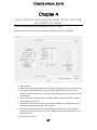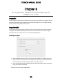
1
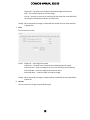
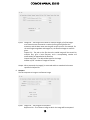
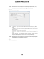
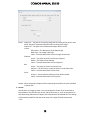
User Manual Version 0.9.16 Written by: Sreya Ghosh, Daqi Dong, Gregorio Lobo, Timothy Mathis and Nurmohammed Patwary based on notes from Einir Valdimarsson and Chrysanthe Preza Edited by: Chrysanthe Preza 2014 Computational Imaging Research Laboratory Electrical & Computer Engineering Dept. The University of Memphis Supported by the National Science Foundation CAREER award DBI-0844682 (C. Preza, PI) Supported by the National Science Foundation CAREER award DBI-0844682 (C. Preza, PI) COSMOS software package: copyright and terms of usage Copyright © 2007 Einir Valdimarsson and Chrysanthe Preza The COSMOS package is free software; you can redistribute it and/or modify it under the terms of the GNU General Public License as published by the Free Software Foundation; either version 2 of the License, or (at your option) any later version. COSMOS is distributed in the hope that it will be useful, but WITHOUT ANY WARRANTY; without even the implied warranty of MERCHANTABILITY or FITNESS FOR A PARTICULAR PURPOSE. See the GNU General Public License for more details. You should have received a copy of the GNU General Public License along with this program; if not, write to the Free Software Foundation, Inc., 59 Temple Place, Suite 330, Boston, MA 02111-1307, USA. Any publications with results obtained with COSMOS should cite COSMOS. COSMOS citations should be made by referring to the COSMOS web page: http://cirl.memphis.edu/cosmos. COSMOS MANUAL (0.9.16) Table of Contents Chapter 1 ......................................................................................................................................... 5 Installation Guide ............................................................................................................................ 5 Downloading COSMOS ............................................................................................................ 5 Windows 7 installation ............................................................................................................ 5 Chapter 2 ......................................................................................................................................... 8 Building COSMOS from source code ............................................................................................... 8 Chapter 3 ......................................................................................................................................... 9 Description of the applications/utilities available in COSMOS ....................................................... 9 Introduction ............................................................................................................................. 9 3.1 COSM Tools ....................................................................................................................... 9 3.2 COSM PSF ........................................................................................................................ 20 3.3 COSM Estimation ........................................................................................................... 265 3.4 COSM Viewer ................................................................................................................... 32 3.5 Command line interface ................................................................................................ 343 Chapter 4 ..................................................................................................................................... 366 How to generate a microscope line-spread function (LSF) using the COSMOS PSF module. ..... 376 Chapter 5 ..................................................................................................................................... 398 How to generate a simulated microscope image using the COSMOS Tools module .................. 398 Introduction ......................................................................................................................... 398 Image formation .................................................................................................................. 398 Chapter 6 ....................................................................................................................................... 41 How to process an image (measured or simulated) using the COSMOS Estimation module ....... 41 Chapter 7 ....................................................................................................................................... 40 An Implemented Example Demonstrating the Various Functionalities of COSMOS .................... 41 Chapter 8 ..................................................................................................................................... 465 An Implemented Example Demonstrating the Depth Variant (DVEM) Algorithm of the COSMOS ..................................................................................................................................................... 465 Generate a test image ......................................................................................................... 465 Generate an LSF................................................................................................................... 476 Create the forward image ................................................................................................... 487 3 COSMOS MANUAL (0.9.16) Restore the original image .................................................................................................. 487 Chapter 9 ....................................................................................................................................... 50 Frequently Asked Questions.......................................................................................................... 50 Chapter 10 ..................................................................................................................................... 52 References ..................................................................................................................................... 52 4 COSMOS MANUAL (0.9.16) Chapter 1 Installation Guid e Downloading COSMOS COSMOS can be downloaded at http://cirl.memphis.edu/cosmos. Download the Package according to system requirements: Cosm-0.9.10-Darwin.dmg - installation package for Mac Tiger 10.4 (executable) Cosm-0.9.10-win32.msi - installation package for Windows XP / win7 (executable) Cosm-0.9.10-win32.zip - archive of COSMOS executables for Windows XP / win7 Cosm-0.9.10.zip - archive of COSMOS source for Windows XP / win7 Cosm-0.9.10.tar.gz - archive of COSMOS source for Linux Cosm-0.9.10-Linux.tar.gz - archive of COSMOS executables for Linux Windows 7 installation The following instructions are for the installation package for Windows 7. 1. Click on the desired file, and then click on Run (shown in the image below) to install. 2. Choose the installation location. Click Next to continue (shown in the image below). 5 COSMOS MANUAL (0.9.16) 3. Click Install to begin the installation (shown in the image below). 4. Click Finish. The folder with the contents of the installation is shown in the image below. 6 COSMOS MANUAL (0.9.16) 7 COSMOS MANUAL (0.9.16) Chapter 2 Buil ding COSM OS from sour ce code Because cmake is used to generate project files (or makefiles), there should not be any changes made to the project file, only to the cmake configuration. The process for building COSMOS for any operating system is the same: 1. Download cmake from www.cmake.org and install. 2. Download Blitz++ from sourceforge.net/projects/blitz/ and install and build. 3. Download fftw from www.fftw.org and install. There are some special instructions for windows to fix the libraries. (www.fftw.org/install/windows.html) 4. Download vtk from www.vtk.org and install and generate project files with cmake and build. 5. Dowload fltk from www.fltk.org and install and generate project files with cmake and build. 6. Download tclap from tclap.sourceforge.net and install and build. 7. Generate the project files for COSMOS with cmake and build. Start the cmake-gui and specify the installation paths for the previously installed packages (2-6) 8 COSMOS MANUAL (0.9.16) Chapter 3 Des cripti on of t he appli cations/ utilities a vail abl e i n COSMOS Introduction All files to be opened and processed in COSMOS require the WASHU header *(.wu) extension. The header is 1024 bytes long. The Add Header Tab available in the COSMOS Tools allows the user to add the WASHU header to a file in the raw format (.raw) and make it a (.wu) file. Only .raw files can be processed by the Add Header. If the image is not a raw image you can convert it to one using the open source software ImageJ (http://rsbweb.nih.gov/ij/download.html). The 4 modules in COSMOS are: 3.1. COSM Tools 3.2. COSM Psf 3.3. COSM Estimation 3.4. COSM Viewer Also, COSMOS now has a command line option: 3.5. Command Line Interface 3.1 COSM Tools The tabs available are: 1. Info This tab shows the header information of the inputted file. 9 COSMOS MANUAL (0.9.16) Inputs: Image file – The desired file. Outputs: Dimension – The dimensions of the image. Data Type – The image’s data type. Size in Bytes – The image size. Maximum – The maximum value of the image. Minimum – The minimum value of the image. Average – The image’s average value. 2. Remove header This tab removes the WASHU header from the image(s). Inputs: Image File – The image from which the WASHU header is to be removed. For multiple images, all of the images must have the same name with a number (starting from 0) before the extension, and the base name must be given as the input file. For example, for the two images Image0.wu and Image1.wu, the filename Image.wu must be given. Output File – The path of the outputted file where the image with the WASHU header removed will be stored. For multiple files, give a base filename, and a corresponding number will automatically be appended to the filename. Number of File – The number of images to covert. Outputs: When executed, the header is removed from the image(s) and the raw image is stored with the name specified in Output File. 3. Add Header This tab adds the WASHU header to a raw image. 10 COSMOS MANUAL (0.9.16) Inputs: Image File – The image to which the WASHU header is to be added. Output File – The file path where the image without the header will be stored. Dimension – The image’s dimensions. Output Data Type – The output image’s datatype. Big Endian – The input image’s byte order (Little Endian if left unchecked). Output: When executed, the header is added to the raw image and is stored with the name specified in Output File. 4. Resample This tab is used to down-sample or up-sample an image. Inputs: Image File – The image to be resampled. Output File – The path to the file where the resampled image will be stored. Factor – The factor by which the image will be resampled. Downsample/Upsample – The desired sampling (down or up). 11 COSMOS MANUAL (0.9.16) Output: When executed, the image is resampled and stored with the name specified in Output File. 5. Transform This tab is used to shift or change the dimensions of an image. Inputs: Image File – The image to be resized. Output File – The path to the file where the resized image will be stored. Output Dimension – The desired new dimensions. Shift – The number of pixels to shift the image. Value Fill – The value of the new pixels generated from shifting the image. Output: When executed, the image is resized and shifted and then stored with the name specified in Output File. 6. Shift This tab shifts an image. Inputs: Image File – The image to be shifted. 12 COSMOS MANUAL (0.9.16) Output File – The path to the file where the shifted image will be stored. Shift – The number of pixels to shift the image. Circular – Perform a circular shift, meaning that the pixels that are shifted off of the image are shifted back around to the other side. Output: When executed, the image is shifted and then stored with the name specified in Output File. 7. Scale This tab scales an image. Inputs: Image File – The image to be scaled. Output File – The path to the file where the scaled image will be stored. Scale with Sum – Scale the image by the sum of all the values (normalization). Scale with Max – Scale the image by the maximum value. Scale with Value – A value by which to scale the image. Output: When executed, the image is scaled and then stored with the name specified in Output File. 8. Convert This tab converts an image to a desired data type. 13 COSMOS MANUAL (0.9.16) Inputs: Image File – The image to be scaled. For multiple images, all of the images must have the same name with a number (starting from 0) before the extension, and the base name must be given as the input file. For example, for the two images Image0.wu and Image1.wu, the filename Image.wu must be given. Output File – The path to the file where the scaled image will be stored. For multiple files, give a base filename, and a corresponding number will automatically be appended to the filename. Output Data Type – The desired data type for the image. Number of File – Number of images to convert. Output: When executed, the image(s) is converted and then stored with the name specified in Output File. 9. Compare This tab compares an image to a reference image. Inputs: Image File – The image to be compared. Reference File – The reference image to which the image will be compared. 14 COSMOS MANUAL (0.9.16) Output: When executed, the two images will be compared, and the maximum, mean, and mean square error between the two images will be displayed. 10. Convolve This tab convolves two images. Inputs: 1st Image File – The first of the two images being convolved (usually an object image). 2nd Image File – The second of the two images being convolved (usually a point spread function). Centered PSF – Convolve two centered PSFs. Output File – The path to the file where the result of the convolution will be stored. Output Image Size – The convolution result’s image size: normal (the two image sizes added together) or the size of one of the inputted images. Output: When executed, the two images will be convolved, and the resulting image will be stored with the name specified in Output File. 11. Object This tab creates objects. 15 COSMOS MANUAL (0.9.16) Inputs: Image File – The path to the existing image that the object will be written onto (Note: Image File should be left blank when creating a new image) Output File – The path to the file where the object will be stored. Create: Dimensions – The dimensions of the blank image. Data Type – The image’s data type. Value – The value with which to fill the image’s dimensions. Ellipsoid: Center – The point on which to center the ellipsoid. Radius – The radius of the ellipsoid. Value – The value with which to fill the ellipsoid. Box: Center – The point on which to center the box. Half-size – The half-size (or radius) of the box in each dimension. Value – The value with which to fill the box. Point: Position – The coordinates where the point will be located. Value – The value with which to fill the point. Output: When executed, the object will be created and stored with the name specified in Output File. 12. Variant This tab forms an image by either a sum of convolutions of each of the strata with an interpolation of the LSFs that are on each side of the strata; or a sum of convolution of each plane along Z dimension of object with components of PCA-Based PSF The settings will be saved into XML file that has same name as the input file with file extension “.xml”. 16 COSMOS MANUAL (0.9.16) Inputs: Object File – The first of the two images being convolved. PSF File – The second of the two images being convolved. PSF number should be deleted. i.e. if there are 50 PSFs (psf0.wu, psf1.wu, … … … , psf49.wu) only first psf should be given as input and 0 (zero) should be removed. Input in this case will be “psf.wu”. For PCA mode PSF file will be number removed first base PSF (same as strata mode). Other necessary files must be in the same folder and COSMOS will automatically read all necessary files. Centered PSF – Convolve two centered PSFs. Output File – The path to the file where the result of the convolution will be stored. Strata mode / PCA mode – Switch between strata mode and PCA mode. Number of Strata – The number of strata the object will be divided into. Start of Strata – The start of the first strata, which is the beginning of the object in terms of z-pixels. Size of Strata – The size of each stratum in pixels. Number of Components – The number of components of PCA-Based PSF files. Start of PSF File – The PSF file for the first PSF defined at the starting depth, which is the top of the object in terms of z-pixels. Number of PSF File – No of z-planes in region of interest (ROI). i.e. if object has dimension 128×128×256 and ROI starts from 100 and ends at 150 then start of PSF file should be 100 and Number of PSF file should be 50. Output: When executed, the two images will be convolved, and the resulting image will be stored with the name specified in Output File. The settings will also be stored in an XML file with the same name as the image. 17 COSMOS MANUAL (0.9.16) 13. PCA This tab transforms original PSF files to PCA-Based PSF files. Inputs: Original PSF File – Specify the original PSF files. PCA-Based File – The Target of PCA-Based files. Number of PSF Files – Number of original PSF files which are used to calculate PCA-Based PSF files. Depth interval between PSFs [pixels] – Set as 1. Any value other than one will be considered as 1. Number of Components –No of component/base PSFs. Generate higher no of component PSFs (i.e more than 50) and any number of component PSFs (i.e. 3/5/7 etc.) can be used for estimation. Higher no of components will increase estimation accuracy. Output: When executed, the new PCA-Based PSFs will be created, which are components, average PSF and coefficient files. Three files will be generated : <name>_PCA_BaseZero (average PSF), <name>_ PCA_coefficients (component PSF weights) and <name> (base PSFs). 18 COSMOS MANUAL (0.9.16) 14. Wavefront encoded (WFE) PSF This tab transforms conventional PSF to WFE-based PSF. Inputs: Conventional PSF – The conventional (original) PSF which needs to be transformed to new PSF. Notes that, this conventional PSF file it must involve certain parameters of PSF’s configuration. These parameters have been added to PSF header file beginning from new version (0.9.7) of COSMOS. Users may need to recreate their PSF files by new COSMOS version if the PSF files were created by older version. Mask File – The Phase Mask file which would be used to produce new WFE-PSF. All zeros around the phase mask should be cropped. Raw phase mask data type should be 32-bit float. For generating bigger dimension WFE-PSF, higher memory (more than 32 GB RAM) may require. If data type or memory requirement does not meet, program may stop executing. Also, the mask must be unwrapped, because when the mask size was changed within the process of CPM-based PSF engineering, the input mask must be a ‘raw’ one, unwrapped; otherwise the final result will be impacted. So we remind the users that don’t do the kind of “phase wrapping” to your mask for this CPMbased PSF engineering process. 19 COSMOS MANUAL (0.9.16) Output: The new WFE-PSF file. 3.2 COSM PSF This module is used to generate the PSFs. The software uses the .xml files to input the settings for PSF generations. However, PSF files can be created according to desired needs by using the GUI. Parameters PSF XML import file XML file that contains stored parameters from a previously generated PSF. This file can be used to obtain multiple images taken under the same conditions. Once the XML file has been selected, click Open to import the settings. Evaluation PSFs can be generated using one of the following evaluations: 20 COSMOS MANUAL (0.9.16) Radial Interpolation: The PSF of discrete points are obtained and interpolated over the system to get the output. Exact evaluation: The PSF is calculated for each point. Although it is very accurate, it has a large overhead. Model There are two models by which the PSFs can be generated: Gibson_Lanni 1992: This is a model for creation of PSFs that tries to effectively model the effects of aberrations in fluorescence light microscopy. For further details refer to [7]. Haeberle: This model is an improvement on the Gibson and Lanni model. This combines the ease of a scalar model with high accuracy. For further details refer to [8]. Type The PSF can be computed according to one of the following microscope types: 2-Photon: It is a fluorescence imaging technique that allows the imaging of living tissue up to a depth of one millimeter. The two-photon excitation microscope is a special variant of the multiphoton fluorescence microscope. Two-photon excitation can be superior due to its deeper tissue penetration, efficient light detection, and reduced phototoxicity. Confocal-circular: By having a confocal pinhole, the microscope is very efficient at rejecting out of focus fluorescent light. The practical effect of this is that the image comes from a thin section of the sample (small depth of field). By scanning many thin sections through the sample, a very clean three-dimensional image of the sample can be built. Confocal-Line: This has the same specifications of a confocal microscope apart from the fact that it has confocal slit rather than a confocal pinhole. Non- Confocal: This is conventional wide-field fluorescence microscopy. DIC: Differential interference contrast microscopy is a phase imaging technique that allows the visualization of transparent unstained objects. Precision: The data precision of the image can be selected as: Single: The PSF generated has 32-bit precision. This is the lowest precision available. 21 COSMOS MANUAL (0.9.16) Double: The PSF generated has 64-bit precision. Long Double: The PSF generated has 80-bit precision. This is the highest precision available. Dimension: The dimensions of the 3D PSF image in pixels. Note: The image space consists of the object space (the pixels occupied by the object) and the background space. Spacing: The spacing (in µm) between the pixels of the 3D PSF image. Note: If the PSF is generated to process an image using a COSMOS algorithm, then these pixel sizes should match those of the image. For experimental data, the XY pixel size is dictated by the camera pixel size and the magnification of the lens. The pixel size along Z is the distance between PSF planes along Z, and it corresponds to the depth at which the lens is focused into the sample. It is the Z step size used when the sequence of 2D optical sections is captured. For simulations, these pixel sizes should be taken based on the Nyquist sampling rate in order to avoid aliasing. Absolute Error: The maximum error allowable during calculations. Lateral Magnification: The objective lens magnification. This value is obtained from the lens used. Numerical Aperture: This is also a direct property of the lens and available on the objective lens. Wavelength: The wavelength (in nm) of the emission filter used to detect the emitted fluorescence light from the sample. Angle Interval: This option is for DIC PSFs only and corresponds to the interval between rotation angles. Thickness Interval: For the Depth Variant Expectation Maximization Algorithm, the Thickness Interval indicates the thickness (in mm) of each slice of the specimen. The interval number is the depth at which the specimen is imaged. It should be a whole multiple of the pixel size. 22 COSMOS MANUAL (0.9.16) Total Number: In the case of the DVEM algorithm, this is the total number of intervals in which the sample is divided. Refractive Index and Thickness: Coverslip These parameters pertain to the coverslip over the object: Design: The designed refractive index and the thickness (in mm) of the coverslip. Actual: The actual refractive index and the thickness (in mm) of the coverslip. Immersion Medium These parameters pertain to the immersion medium (oil, air, or water) of the lens: Design: The designed refractive index and the thickness (in mm) of the immersion medium. Actual: The actual refractive index and the thickness (in mm) of the immersion medium. Specimen These parameters pertain to the specimen: The average refractive index (no units) and the thickness (in mm) of the specimen. OTL These parameters pertain to the OTL (optical tube length): Design: The designed optical tube length (in mm). Actual: The actual optical tube length (in mm). Confocal: Note: The field of confocal microscopy has been rapidly progressing. COSMOS cannot compute PSFs for more recent confocal microscopes. The following are parameters for computing a confocal PSF. This section is only valid for those using Confocal Microscopy: Size: The size of the confocal pinhole. Distance: The length of time the laser dwells on the specimen. 23 COSMOS MANUAL (0.9.16) Magnification: The magnification of the image. DIC: Note: COSM PSF’s DIC support is still under development and is not currently functional. The following are parameters for computing a DIC (differential inference contrast) PSF. Detail information about the PSF can be found in [13]. This section is only valid for those using DIC Microscopy: Shear: The shear distance due to the Wollaston prism. Bias: The constant phase introduced by moving one of the prisms. Amplitude Ratio: For crossed polars the amplitude is 0.5 for each component of the shear beam. Rotation Angle: The angle that the shear direction makes with the horizontal axis. Sum over Y: Used to collapse the PSFs over the Y dimension to create LSFs. Uncentered: Used to create an uncentered PSF file. However, centered PSFs are more common. PSF Filename: The path where the PSF image will be stored in the WASHU (.wu) format. Generate Real and Imaginary: Used to generate both the real and imaginary PSFs. If unchecked, only the intensity PSF will be created. Automatically import configurations from XML file Normally, CosmPsf recalls default configurations when it starts, but if there is a file of “lastest.xml” in the same folder of CosmPsf, then content of “lastest.xml” will be recalled automatically as customized configurations. This function is useful to the user who wants to use special configurations which are not default. To use this function, copy the xml file to the folder containing CosmPsf, and change the file’s name to “lastest.xml”. To undo this function, simply delete or rename “lastest.xml”. 24 COSMOS MANUAL (0.9.16) 25 COSMOS MANUAL (0.9.16) 3.3 COSM Estimation Using the COSMOS to obtain images using the above algorithms: The image from the microscope is given in Data Input File. The corresponding PSF is given in PSF Input File. Parameter: The parameter is a value from 0 to 1.When given the correct parameter, we get the output close to the original object. This is mainly a trial and error method. This helps to remove artifacts. The output gets stored by the name given in Estimated Output File. Parameters XML File XML file that contains stored parameters from a previous estimation. This file can be used to perform the same or similar estimation multiple times. Once the XML file has been selected, click Open to import the settings. Data Input File The image from the microscope. PSF Input File The PSF corresponding to the Data Input File. Centered PSF Perform the estimation using a centered PSF. Estimation Output File The path where the result of the estimation will be stored. Linear Method Parameters: 26 COSMOS MANUAL (0.9.16) Linear Least Squares (LLS) This is a one-step algorithm that yields solutions in a few seconds that are optimal in the least squares sense. Results from sensitivity studies show that the proposed method is robust to noise and to underestimation of the width of the point-spread function. The method is particularly useful for applications in which processing speed is critical, such as studies of living specimens and time lapse analyses. [2] Linear Maximum a Posteriori (MAP) This approach also yields a regularized linear estimator which reduces noise as well as edge artifacts in the reconstruction. The advantage of the linear MAP estimate over the LLS is its ability to regularize the inverse problem by smoothly penalizing components in the image associated with small Eigen values. [3] Parameter A value from 0 to 1.When given the correct parameter, an output close to the original object can be obtained. This is a trial and error method which helps to remove artifacts. Iterative Method Parameters: Iterations The number of iterations for the algorithm to be executed. Update 27 COSMOS MANUAL (0.9.16) The number of iterations before the terminal window is updated Write The number of iterations before the maximum, minimum, and mean values is printed to the terminal. Invariant: Expectation Maximization(EM) This strata-based model incorporates spherical aberration that worsens as the microscope is focused deeper under the cover slip and is the result of the refractive-index mismatch between the immersion medium and the mounting medium of the specimen. Images of a specimen with known geometry and refractive index show that the model captures the main features of the image. [5] Jansson-van Cittert (JVC) This is an iterative deconvolution algorithm. The advantage of such a method is that the process is fairly stable in the presence of noise and error when compared to the non-iterative deconvolution. [4] Penalty 28 COSMOS MANUAL (0.9.16) A value between 0 and 1 used for noisy simulations. Simulation can either be done with Intensity or Roughness penalty. In invariant section, current version (0.9.10) only supports the Expectation Maximization (EM) algorithm. Double Z As this is an invariant estimation, there is only one PSF. Double Z dimension must be selected while executing these two algorithms. Variant: Data input file Blurred WU image. PSF input file First PSF file name. PSF number should be removed. (See section 3.1.12) Space-variant EM (EMSV) This is a depth variant algorithm with the variations in the z dimension assumed to be a minimum. 29 COSMOS MANUAL (0.9.16) Ordered Subsets EM (EMOS) This algorithm is still under development. DV Conjugate Gradient (DVCG) This is a depth variant maximum likelihood restoration using a conjugate gradient algorithm Penalty A value between 0 and 1 used for noisy simulations. Simulation can either be done with Intensity or Roughness penalty. In variant section, current version (0.9.10) only supports Space-Variant EM algorithm with strata/PCA mode. Double Z Double Z dimension must be selected while executing EMSV or EMOS algorithms. Strata Number of strata (usually the number of PSFs minus one). Start The starting depth of the first PSF. Size The number of planes in each stratum. OTF Name The path to the optical transfer function if OTF on Disk is selected. Otherwise, OTFs are automatically generated by the program, so OTF in Memory is usually selected. Strata mode / PCA mode Switch between strata and PCA mode. Components Number of components of PCA-Based PSFs. Start 30 COSMOS MANUAL (0.9.16) Stating plane number of object ROI (see Section 3.1.12) The number of PCA-Based PSFs which are used to do inversing. Convergence: The graph can be plotted here for various parameters with the simulations and the reference file. Various things can be computed here such as IDIV values, MSE, maximum, minimum, mean. Reference File The image with which the estimation will be compared. If left blank, the previous estimation will be used. Measure The values to be computed during the comparison. Table The table containing the values computed during the comparison. These values can be saved as .csv file by clicking Save. Clear 31 COSMOS MANUAL (0.9.16) Clears the plot in the measurement graph area. maximum The maximum value on the vertical axis. minimum The minimum value on the vertical axis. Generation and Processing of a 2D XZ image using the Depth Variant (DV) Approach 1. Forward Image Formation (DV) The Depth-Variant model assumes that a point source in the object will have a PSF depending on its depth in the object. The more PSFs we would use the better, but unfortunately, by increasing the number of PSFs we also increase the computational complexity of the estimation algorithm. A middle ground is to pick a several depths that we will generate a PSF and divide the object into parts that we call strata. 2. PSF Generation (Line Spread Function) The CosmPsf application is started. If we want n strata we generate n+1 PSFs, 1 each for the boundary of each stratum. In the CosmPsf application, we can specify how many PSF we will generate and the Thickness (Depth) intervals. The depth interval is determined by the spacing in z and how many pixels in z we have in each stratum. Normally, the CosmPsf application would generate a 3-D PSF, but we can force it to collapse the Y dimension (sum over it) into a single plane by enabling “Sum over Y”. The resulting PSF is a 2-D image often referred to as Line Spread Function (LSF). Specify the name of the resulting LSF. The application will append a number to the filename before the file extension. Press Generate and the LSFs will be generated one after the other. 3. Image Formation (DV) The image formation for the Depth Variant model is a sum of convolutions of each stratum with an interpolation of the PSFs that are on each side of the strata. Start the ComsTools application and select the Variant tab. We specify the object file name and specify the PSF name without the last number next to the extension. The output filename needs to be specified. The user needs to specify 3 parameters: the number of strata, the start of the first strata, which is the beginning of the object in z pixels. Press Execute, and the image will be generated. 4. Image Estimation (DV) Depth-Variant Expectation Maximization (DV-EM) algorithm This image and a single LSF can be used to estimate the object using the LLS, MAP, and EM algorithms, but the resulting estimation will not be quite like our original object. The 32 COSMOS MANUAL (0.9.16) image can be estimated by using the EM Space Invariant Algorithm. The COSM Estimation needs to be started, and the Iterative tab and the Variant sub-tab need to be selected. Enable the EMSV algorithm. Specify the image file name, the LSF, and the output filename. Then specify number of iterations and how often to update and write. The algorithm will process the image upon pressing run. 3.4 COSM Viewer COSM viewer is used to display images in 3D cut view. 3D viewing 3D view rotation (upper left portion) can be activated by pressing the ‘t’ key. After that, the graph can be rotated by clicking and dragging the graph. 2D viewing 2D images are displayed at the bottom of window. The planes can be traverse using the Z, Y, and X sliders at the bottom of the window. The brightness and contrast can be adjusted using the vertical sliders on the lower right portion of the window. Graphing Graph 33 COSMOS MANUAL (0.9.16) Plots the intensity profile of the image in the graph portion of the screen (upper right) Clear Clears the graph. Scale Plots the intensity profile in either Linear or Logarithmic scale. Intersection Decides which planes to plot on the graph. XY and XZ intersection implies that Z is in the vertical and Y is in the horizontal axis. Similarly, XY and YZ intersection implies that Z is in the vertical axis and X is in the horizontal axis. In the same way, XZ and YZ intersection implies that Y is in the vertical axis and X is in the horizontal axis. To compare two images, open the first image and click Graph. Then open the second image and click Graph. The graph will retain the plot of the previous image. 3.5 Command line interface Command line interface (CLI) runs Cosmos applications by commands without the GUI. CosmEstmation and CosmPsf support CLI because these 2 parts are normally time-consuming. Benefits of using CLI Multiple jobs could be maintained and executed together automatically; CLI displays job status timely in running time. This is useful to the user who is running a time-consuming job (more than 4 hours). COSM Estimation CLI Usage CLI is enabled using the --cli (or -c) option, as shown below: CosmEstimation --cli [other options] The following is a typical way of using COSM Estimation CLI: 34 COSMOS MANUAL (0.9.16) CosmEstimation --cli --img <PATH AND FILENAME OF FWD FILE> --psf <PATH AND FILENAME OF PSF FILE> --est <PATH AND FILENAME OF OUTPUT FILE> --update 100 --em 1000 –write 100 –-double Options The description of all options: --cli (or -c): Switch to use CLI function. --img (or -t): Set value of forward image’s filename. --est (or -t): Set value of estimation file’s filename. --psf (or -p): Set value of PSF file’s main filename. --otf (or -f): Set value of OTF file’s main filename. Default value is ‘otf’. --pha(or -y): Set value of Phantom file’s main filename. Default value is ‘pha’. --suffix (or -x): Set value of above files’ external filename. Default value is ‘wu’. --update (or -u): Set value of number of iterations between statistics updates. Default value is 100. --write (or -w): Set value of number of iterations between write updates. Default value is 100. --lls (or -l): Set value of LLS estimate. Default value is 1E-4. --map(or -m): Set value of MAP estimate. Default value is 1E-4. --em (or -e): Set value of iterations of either EM, EM-SV or EM-OS. Default value is 100. --jvc (or -j): Set value of iterations of JVC. Default value is 100. --sv (or -v): Switch to use EM-SV estimation algorithm. --os (or -o): Switch to use EM-OS estimation algorithm. --num (or -n): Set value of number of strata (stata mode) / number of components (PCA mode). Default value is 1. --start (or -s): Set value of start of strata (strata mode) / starting z-plane of ROI (PCA mode). Default value is 1. (see section 3.1.12) --size (or -k): Set value of size of strata (strata mode) / end z-plane of ROI (PCA). Default value is 1. (see section 3.1.12) --double (or -d): Switch to use double Z dimension. ( for EM-algorithms z dimension must be doubled). --intensity (or -I): Set value of Intensity penalty. Default value is 0. --roughness (or -R): Set value of roughness penalty. Default value is 0. --err (or -E): Set value of error estimation, Default value is “0x1f”. --center (or -C): Set value of whether it is using centered PSF file. Default value is 1, using centered PSF; otherwise it’s 0, not using (true). --table(or -a): Set value of error information’s filename --pca(or -P): Switch to use PCA mode. (Default is strata mode) 35 COSMOS MANUAL (0.9.16) COSM PSF CLI Usage CLI is enabled using the --cli (or -c) option, as shown below: CosmPsf --cli [other options] The following are typical ways of using COSM PSF CLI: CosmPsf --cli --file <PATH AND FILENAME OF PSF INPUT XML FILE> or CosmPsf --cli --file < PATH AND FILENAME OF PSF INPUT XML FILE > --interval 0.0001 --total 5 Options The description of all options: --cli (or -c): Switch to use CLI function. --file(or -f): Set value of input PSF XML file path. Default value is “psf.xml”. --double (or -d): Switch to use double precision. (Not support yet. Only supports to using float precision now). --long (or -l): Switch to use long double precision. (Not support yet. Only supports to using float precision now) --interval (or -i): Set value of PSF Thickness Interval. Default value is 0. --total (or -t): Set value of PSF total number. Default value is 1. --sum (or -s): Switch to do sum over Y. --uncentered (-u): Switch to not use centered PSF file. --gri (-g): Switch to do generate real and imaginary. COSM Tools CLI (WFE) In current version, CLI is activated only for WFE tab. CosmTools --cli --input <conventional PSF file name and path name> --reference <mask file name and path name > --output <output: WFE-PSF file name and path name > --cpm 36 COSMOS MANUAL (0.9.16) Chapter 4 How t o generat e a mic ros cope li ne -s pread function (L SF) usi ng the COSMOS PSF mod ule. The PSFs can be generated using the COSM PSF steps in this chapter. There are default values present in the window that will be used for the simulations. 1. Open CosmPsf. 2. Select Exact Evaluation for better results though only marginally more time consuming. 3. The image will be devided into 10 parts. The ring is divided into 8 parts with a part above and a part below the ring. Therefore, 9 PSFs will be generated. So, 9 is entered in Total Number. 4. The size between pixels (Spacing) is specified as 0.06 µm, and the number of pixels in each stratum is chosen as 5. 5. The depth interval (Thickness Interval) is chosen as 0.0003 mm. This depends on the spacing in z and number of pixels in each stratum. 6. Normally the CosmPsf application would generate a 3D PSF, but it can be forced to collapse the Y dimension (sum over it) into a single plane by enabling Sum over Y. This 2D PSF is the LSF. 7. The rest of it is left as is. 37 COSMOS MANUAL (0.9.16) 8. The output file (PSF Filename) is entered. The generation of the LSF produces the following XML file: <?xml version="1.0"?> <!-- PSF specification file --> <!-- model = <"Gibson_Lanni1992" | "Haeberle" > --> <!-- eval = <"Interpolation" | "Exact"> --> <!-- type = <"Non-confocal" | "Circular-confocal" | "Line-confocal"> --> -<PSF version="" unit="mm" spacing="6e-005 6e-005 6e-005" dimension="64 64 64" file="C:\Users\timathis\Desktop\psf0.wu" precision="Single" type="Non-Confocal" eval="Exact" model="Gibson_Lanni1992"> <AbsoluteError value="0.000001"/> <LateralMagnification value="40.000000"/> <NumericalAperture value="1.000000"/> <Wavelength unit="mm" value="0.000580"/> -<CoverSlip> <RefractiveIndex Actual="1.522000" Design="1.522000"/> <Thickness unit="mm" Actual="0.170000" Design="0.170000"/> </CoverSlip> -<ImmersionMedium> <RefractiveIndex Actual="1.515000" Design="1.515000"/> <Thickness unit="mm" Actual="0.160000" Design="0.160000"/> </ImmersionMedium> -<Specimen> <RefractiveIndex value="1.330000"/> <Thickness unit="mm" value="0.000000"/> </Specimen> <OTL unit="mm" Actual="160.000000" Design="160.000000"/> </PSF> 38 COSMOS MANUAL (0.9.16) Chapter 5 How t o generat e a sim ulated micros cop e im age usi ng t he COSMOS Tools m od ule Introduction In order to test the performance of algorithm, the generation of simulations is required. We can simulate a microscope image using two sub tabs from the COSM Tools, i.e. the Object sub tab and the Variant sub tab/Convolution sub tab. Image formation To simulate a microscope image an object and a PSF are necessary (see the previous chapter). The image is formed when the object and the PSF are convolved. This can be done using the convolution tab or the variant tab in the case of the DVEM Algorithm. Creating an object 1. Go to the Object sub tab. In Create you can enter the output file; the input file can be left blank. Input the Dimensions of the image and the Data Type. Value represents the color fill (0 indicates a black background while 1 represents white). 2. Go to the tab specifying the shape desired. Here the ellipsoid tab is chosen with center as (64, 64, and 64) and radius 8. The object can be viewed in COSM Viewer: 39 COSMOS MANUAL (0.9.16) Creating a forward image 1. Open the variant sub tab of the CosmTools. 2. The object and PSF (generated using the method in the previous chapter) are convolved using the convolution tab in COSMOS Tools. The simulated microscope image can be viewed in COSM Viewer: 40 COSMOS MANUAL (0.9.16) Chapter 6 How to p roces s a n im age (m eas ur ed or si mul ated) usi ng the COSMOS Estim ati on m od ule The same PSF generated for the forward image in the previous chapter needs to be used for the estimation process. 1. 2. 3. 4. 5. Open COSM Estimation Select the Data Input File as the forward image created in the previous chapter. Select the PSF Input File as the PSF convolved with the object in the previous chapter. Specify where the Estimation Output File will be stored. Select an algorithm (See 3.3 COSM Estimation for information about the algorithms used in COSMOS). If a Linear algorithm is selected, the image can be processed immediately by clicking Run. If an Iterative algorithm is selected, there are a number of parameters that need to be entered depending on the options that the chosen algorithm requires. 6. Click Run. 41 COSMOS MANUAL (0.9.16) Chapter 7 An i mpl em ent ed ex ampl e demonstrati ng a sim ulation of the for wa rd a nd i nver se s pa c e-invaria nt ima ging COSM p r oblem using t he COSM OS functionaliti es 1. The image is chosen as a hollow ring with two intersecting axes (128,128,128). 2. The PSF is created from the CosmPsf Module. 3. The simulated microscope using The COSM Tool convolves. 42 COSMOS MANUAL (0.9.16) 4. The Estimated microscope image. 5. The image is estimated using COSM Estimation. For example using the EM Algorithm for 1000 Iterations or more. 43 COSMOS MANUAL (0.9.16) 6. The Image after 1000 iterations. 7. The image viewed in COSM Viewer after 10000 iterations. 44 COSMOS MANUAL (0.9.16) 45 COSMOS MANUAL (0.9.16) Chapter 8 An i mpl em ent ed ex ampl e demonstrati ng a sim ulation of the for wa rd a nd inver se dd ept h- vvaria nt ima ging COSM p r oblem using COSM OS functi onalities Generate a test image Note the following example uses 2D XZ images and LSFs to reduce the dimensionality of the imaging problem to allow quick processing of the image. Create a ring object using the object sub tab in the COSM Tools: 1. Open the Object sub tab in COSM Tools. 2. Open the Create sub tab. Enter the following information: Image File: Leave blank. Output File: The path where the object will be stored. Dimensions: (128, 1, 256) Data Type: Float 3. Click Execute. A blank object was created. 4. Click on the Ellipsoid tab. Enter the following information: Image File: The path to the blank object just created (Same as Output File) Center: (64, 1, 128) Radius: (20, 20, 20) Value: 1 (This indicates that the circle will be white.) 5. Click Execute. This generated a white circle in plane XZ with radius 16. 6. Change the parameters in the Ellipsoid tab to the following: Center : (64, 1,128) Radius: (10, 10, 10) Value: 0 (This indicates black.) 7. Click Execute. This generated a black circle in the middle of the previously generated white circle, creating a ring. The resultant object can be seen in COSM Viewer: 46 COSMOS MANUAL (0.9.16) Generate an LSF An LSF can be created using the steps in Chapter 4 using (256, 64, 128) for the Dimension parameter. The LSF can be seen in COSM Viewer: 47 COSMOS MANUAL (0.9.16) Create the forward image 1. Open the Variant sub tab in COSM Tools. 2. Specify the following parameters: Object File: The path to the ring object. PSF File: The path to the LSF. Output File: The path where the forward image will be stored. Number of Strata: 8 Start of Strata: 108 Size of Strata: 5 3. Click Execute. The forward image can be seen in COSM Viewer: Restore the original image 1. Open COSM Estimation 2. Click the Iterative sub tab and then the Variant sub tab. This is chosen for the best estimation. 3. Select the EMSV algorithm (the DVEM algorithm). 4. A penalty is not necessary since the image in this experiment is a phantom. Real images are noisy, and, hence, a penalty is used. 5. Enter the following information: 48 COSMOS MANUAL (0.9.16) Data Input File: The path to the forward image. PSF Input File: The path to the LSF. Output File: The path where the restored image will be stored. Strata: 8 Start: 108 Size: 5 pixels 6. Click Run. The image improves with increased number of iterations. The estimated output after 1000 iterations: The estimated output after 50,000 iterations: 49 COSMOS MANUAL (0.9.16) 50 COSMOS MANUAL (0.9.16) Chapter 9 Fr eq uently As ked Questions 1. Can I modify or redistribute COSMOS? The COSMOS package is free software; you can redistribute it and/or modify it under the terms of the GNU General Public License as published by the Free Software Foundation; either version 2 of the License, or (at your option) any later version. COSMOS is distributed in hopes that it will be useful, but WITHOUT ANY WARRANTY without even the implied warranty of MERCHANTABILITY or FITNESS FOR A PARTICULAR PURPOSE. See the GNU General Public License for more details. 2. How to debug a process, if a run time error occurs? All compile time error and comments show up in the command prompt, so going back the cause of the error can be found out. This is particularly important when there are multiple iterations being implemented and an error occurs. 3. Can a file in .tiff format be read by the COSMOS? No, but it can be converted to the .wu format using the COSMOS Tools, which can open several different formats. Only .wu format files (i.e. images with a 1024 washu header) can be read by the other applications which are a part of the COSMOS package. Images with no header are usually named with a .raw extension, which can be read by the add header tab in Cosm Tools. This tab adds the washu header and converts the file to .wu extension. 4. What are the system requirements? 1.11 KB of Hard Disk space is required. COSMOS can run on a variety of Operating Systems. 5. Is it possible to process a 2-D image using the LLS or EM algorithms? If so, how are the parameters set in the "COSM PSF" menu? Yes, the number of planes in Z equal to 1. The rest of the parameters are kept as they are. 6. If images are saturated can they still be processed with the COSMOS algorithms? Yes, the intensities will be scaled down, but it can easily be processed with some losses. 51 COSMOS MANUAL (0.9.16) 7. What does "pixel size in object space" in the "Generate PSF" menu mean? Is it the size of a single element of the CCD camera or the size of a single pixel of the image acquired by the CCD camera? Pixel size in object space is equal to the physical CCD pixel size divided by the magnification of all the lenses between the specimen and the camera. For most microscopes, the only lens between the specimen and the camera is the objective lens. For other microscopes, there may be an additional relay lens that further magnifies the image to the camera. 8. When I publish results generated with COSMOS, which of your papers should I reference, and how do I cite the COSMOS package? COSMOS citations should be made by referring to the COSMOS web page (http://cirl.memphis.edu/cosmos). In addition, depending on which algorithm you used to process your images you should cite the publication describing the algorithm. A list of all the algorithms implemented in COSMOS and the references for each algorithm are provided on the COSMOS web page. 52 COSMOS MANUAL (0.9.16) Chapter 10 References 1. Preza, C. and Conchello, J-A., “Depth-variant maximum-likelihood restoration for threedimensional fluorescence microscopy,” J. Opt. Soc. Am. A., 21:1593-1601, 2004. 2. Preza, C., Miller, M. I., Thomas, Jr., L. J., and McNally, J. G., “Regularized linear method for reconstruction of three-dimensional microscopic objects from optical sections,” J. Opt. Soc. Am. A., 9(2):219-228, 1992. 3. Preza, C., Miller, M. I., and Conchello, J.-A., “Image reconstruction for 3-D light microscopy with a regularized linear method incorporating a smoothness prior,” in Biomedical Image Processing and Biomedical Visualization, R. S. Acharya and D. B. Goldgof, Eds., Proc. SPIE 1905:129-139, 1993. 4. Agard, D. A., ‘‘Optical sectioning microscopy,’’ Annu. Rev. Biophys. Bioeng. 13:191–219, 1984. 5. Conchello, J.-A., "Super-resolution and convergence properties of the expectationmaximization algorithm for maximum-likelihood deconvolution of incoherent images", J. Opt. Soc. Am. A, 15:2609-2620, 1998 6. Murphy D.B, “Fundamentals of Light Microscopy and Electronic Imaging”, Wiley LISS, 2001. 7. Gibson, S. F. and Lanni, F., “Experimental test of an analytical model of aberration in an oil-immersion objective lens used in three-dimensional light microscopy,” J. Opt. Soc. Am. A., 9:54–66, 1992. 8. O. Haeberlé, “Focusing of light through a stratified medium: a practical approach for computing microscope point spread functions. Part I: Conventional microscopy,” Opt. Commun. 216, 55-63, 2003. 9. Myneni, V. and Preza, C., “Computational depth-variant imaging for quantitative fluorescence microscopy,” in Computational Optical Sensing and Imaging (COSI), OSA Technical Digest (CD), Optical Society of America, paper # CThC4, 2009. 10. Myneni, V., “Performance Analysis of a Depth-Variant Expectation Maximization Algorithm for 3D Fluorescence Microscopy,” MS Thesis in Electrical and Computer Engineering, the University of Memphis, 2009. 11. Preza, C. and Myneni, V., “Quantitative depth-variant imaging for fluorescence microscopy using the COSMOS software package,” in Three-Dimensional and Multidimensional Microscopy: Image Acquisition and Processing XVII, BIOS, SPIE 7570-2, January 2010. (in press) 12. Markham, J. and Conchello, J.-A., “Tradeoffs in regularized maximum likelihood image restoration,” Proceedings of SPIE 2984, 136-145, 1997. 13. Preza, C., Snyder, D. L., and Conchello, J.-A., “Theoretical development and experimental evaluation of imaging models for differential-interference-contrast microscopy,” Journal of the Optical Society of America A, 16(9):2185-2199, 1999. 53