Download The Space Envelope Representation for 3D Scenes Chapter 4

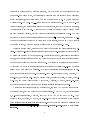
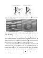
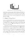
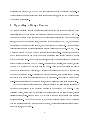
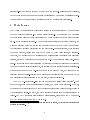
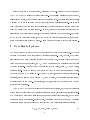
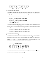
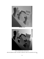
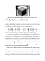
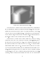
The following is taken from
The Space Envelope Representation for 3D Scenes
Chapter 4: RANGE CAMERAS
of Adam Hoover's PhD dissertation
full copy available at
http://marathon.csee.usf.edu/hoover/home-page.html
1
CCD
im 2D
ag
e
?
?
?
capturing an intensity image
1
LRF
im2 2 D
ag
e
distance=2 meters
distance=1 meter
capturing a range image
(laser range finder)
Figure 1: Illustration of the nature of capturing a range image (of the laser radar variety),
as compared to capturing an intensity image.
1 Introduction
A range camera is a device which can acquire a raster (two-dimensional grid, or image) of
depth measurements, as measured from a plane (orthographic) or single point (perspective)
on the camera. Figure 1 illustrates the nature of the data captured by a range camera, as
compared to a standard CCD (charge coupled device) camera. In an intensity image, the
1
In fact, the camera may consist of several separate components (such as a CCD and light projector, or
two CCDs, or laser and optics and power supply, etc.), but collectively the components make up a single
range camera.
1
2
greyscale or color of imaged points is recorded, but the depths of the points imaged are
ambiguous. In a range image, the distances to points imaged are recorded over a quantized
range (for instance, range value zero may mean a distance of 0 to 2.5 cm, range value one
a distance of 2.5 cm to 5.0 cm, ..., range value 255 a distance of 637.5 cm to 638 cm). For
display purposes, the distances are often coded in greyscale, such that the darker a pixel is,
the closer it is to the camera. A range image may also be displayed using a random color
for each quantized distance, for easy viewing of isodistance quantization bands. The data
acquired by a range camera is often referred to as being \2 -D in nature, as opposed to 3-D.
This is to dierentiate this type of device from other sensors, such as an MRI (Magnetic
Resonance Imager), which can acquire measurements in a complete 3-D grid.
Currently (Spring 1996), there are two major types of range cameras available commercially. A consumer-oriented (less technical) review of range data-acquiring products produced
by fteen companies may be found in [17]. A laser radar camera, also called a laser range
nder, uses a single optical path and computes depth via the phase shift (continuous scan)
or time delay (pulse) of a reected laser beam. The raster of measurements is produced
by sweeping the beam in equiangular increments across the desired eld-of-view (typically
around 60 60) using two mirrors . The image acquisition scenario illustrated in Figure 1 is for a laser radar camera. Odetics Inc. (1515 S. Manchester Avenue, Anaheim, CA
92807-2907), Perceptron Inc. (23855 Research Drive, Farmington Hills, MI 48335, tel 313478-7710), and Laser Atlanta (6015D Unity Drive, Norcross, GA 30071, tel 404-446-3866)
are three companies which produce commercially available laser radar cameras.
A structured light scanner uses two optical paths, one for a CCD and one for some form
of projected light, and computes depth via triangulation. ABW (GmbH, Gutenbergstrasse
9, D-72636 Frickenhausen, Germany, tel (+49) 70 22 / 94 92 92) and K2T Inc. (One
Library Place, Duquesne, PA 15110, tel 412-469-3150) are two companies which produce
commercially available structured light scanners. Both of these cameras use multiple images
1
2
2
See the URL http://www.epm.ornl.gov/jov/range-pages/range-camera.html for a more detailed
illustration.
2
3
ACQUIRING IMAGE ONE
no light
light
object
light
projector
ACQUIRING IMAGE TWO
CCD
object
light
projector
CCD
Figure 2: The rst two striped light patterns used by the K2T GRF-2 structured light
scanner to determine depth.
image of pattern 3 (of 8)
image of pattern 5 (of 8)
Figure 3: Example images of two of the eight structured light patterns used by the K2T
GRF-2 range camera.
of striped light patterns to determine depth, as illustrated in Figure 2. For instance, if a
pixel appears dark in image one, then bright in image two, this indicates the object point lies
within the second fourth of the eld-of-view of the light projector. Two example structured
light patterns used by the K2T GRF-2 range camera are shown in Figure 3.
Both of these types of cameras also capture a form of intensity image in the course of
their normal operation. For the laser radar type camera, the intensities recorded are the
amplitudes of the portion of the beam reected back towards the camera. Since laser radar
cameras use light wavelengths far outside the visible spectrum, it is this author's preference to
refer to the amplitude of the returned energy as reectance. In contrast, the CCD component
4
CCD
50cm
light
projector
50cm
imaging
area
30cm
120cm
Figure 4: Setup for the K2T range camera (side view).
of structured light scanners records visible wavelength amplitudes, commonly referred to as
intensity. In both cases, the reection/intensity image is registered to the range image. The
registration of two images means that at any pixel (r ; c ) in image one, and at any pixel
(r ; c ) in image two, if r = r and c = c then the measurements were made upon the
same point in the scene.
1
2
2
1
2
1
1
2
2 Setting Up a Range Camera
The main components of a laser radar camera (the laser and optics) are typically contained
within one housing. Because this type of camera uses only one optical path, the camera
may essentially be placed anywhere. This author has performed experiments using an Odetics LRF mounted upon the HERMIES-III mobile robot[16], and using a Perceptron LRF
mounted upon an optics workbench.
The relative placement of the components of a structured light type range camera depends
upon the size of the scene to be imaged (and also, of course, upon the eld-of-view limitations
of the light projector and CCD). Figure 4 illustrates a side view of the setup this author
used for experimenting with the K2T structured light camera. The imaging area is roughly
the size of a 15 cm cube. The positions of the CCD and light projector may be swapped.
Support materials for the components should be as stable as possible, while also allowing
some control in tilt. Note that the light stripe patterns for the K2T range camera are
5
horizontal (see Figure 3), so the CCD and light projector should be displaced vertically. If
the light stripes for a given structured light scanner are vertical, then the components should
be displaced horizontally.
3 Operating a Range Camera
The primary operating concern of a structured light range camera is to set a threshold which
will discriminate between lighted and unlighted areas in the images captured by the CCD.
There are ve factors which contribute to the thresholding process: the amount of ambient
light, the power of the projected light, the setting of the aperture on the CCD, the reective
properties of the surfaces being imaged, and the setting of the threshold. The harmonious
collaboration of all ve factors is essential to acquire quality range imagery. The K2T GRF2 unit can project up to 500 watts of standard incandescent light. This amount seems to
work well under roughly 100 watts of ambient uorescent light located roughly 3 meters
above the imaging area. Under these conditions, natural woods (unstained and unpainted)
reect the light patterns to the CCD crisply. Less reective materials, such as cloth, require
that the CCD aperture be more open than for woods. These types of materials can also be
imaged with little or no ambient light, by closing the aperture somewhat or by reducing the
power of the projected light. Materials with higher reectivity, such as plastics and metals,
are best imaged under a substantial amount of ambient light. This helps to wash out any
cross-surface reections of the projected light, giving a crisper pattern after thresholding.
The best process for discovering good settings for all of the illumination factors is to
examine the appearance of the projected patterns in the captured CCD images. A live
television hookup, along with the capability to continuously cycle the light patterns, greatly
facilitates this process. Figure 5 shows CCD images of the same light pattern with dierent
aperture settings. Note that if the human eye cannot visually discern a good threshold
between the illuminated and dark parts of the pattern, a thresholding algorithm likely cannot
either (at least, not robustly).
6
(a) too bright
(b) too dark
(c) aperture set correctly
Figure 5: In image (a), the aperture is too open, discernible by the wash-out of the pattern
in the upper left and right of the image. In image (b), the aperture is too closed, discernible
by the disappearance of the pattern on the top of the cube. Patterns should appear as in
image (c).
Laser radar cameras typically use light wavelengths far outside the visible spectrum (Odetics uses 820 nm, Perceptron uses 835 nm). Thus the eects of ambient lighting (impossible
to see with the naked eye) may be ignored so long as the laser power is sucient. Interestingly, the reectance properties of materials dier at these wavelengths from how they
react to visible spectrum wavelengths. For instance, printed text does not show up at all at
these wavelengths. More importantly, highly reective surfaces can cause problems. This is
because not enough of the outgoing beam may scatter, upon impact with the surface, in the
direction back towards the range camera.
A laser radar camera typically can acquire a range image in under one second, while a
7
structured-light camera can take as much as ve to ten seconds. During image acquisition,
both of these types of cameras must remain motionless and be imaging motionless objects.
This is because the raster of range measurements is not measured simultaneously.
4 Data Issues
The Odetics LRF quantizes the phase shift measured at each pixel of its 128 128 image into
256 depth values covering its 9.4 meter ambiguity interval. The Perceptron LRF quantizes
the phase shift measured at each pixel of its 512 512 image into 4092 depth values covering
its 9.4 meter ambiguity interval. The ambiguity interval (plus the stando distance, the
minimum distance which the camera can measure) denes the depth which the modulated
wave travels and returns while making one complete phase. Past this distance, depth readings
become ambiguous, cycling from zero to the maximum depth value again, ad innitum.
(However, the amplitude of the returning beam still typically diminishes with increased
distance, as can be witnessed in the reectance image.) These pixels are called wrap-around
pixels. Although in theory these pixels can be converted to valid depth readings by adding one
(or more) ambiguity interval distance(s), the stability of these readings is often questionable.
This is due not only to the much-reduced power of the bounced wave, but also due to the
increased chance of cross-reection (the measurement of a signal which has bounced o two
or more surfaces before returning to the camera), at greater distances.
The K2T GRF-2 structured-light camera makes use of 8 striped light patterns . Thus
at each pixel, there are 256 possible light codings, and hence depth readings. However,
the actual depth corresponding to a light coding is dierent from pixel to pixel, because of
the dierences in angles. In eect, the depth readings therefore span a continuous range of
values. The ABW structured light scanner works similarly, producing a 512 512 image.
The K2T scanner produces a 640 480 image.
3
In order to reduce noise, all the patterns are also imaged in reverse, but this does not increase range
measurement precision.
3
8
Because there are two optical paths, occlusion may occur. Parts of the scene visible to
the CCD may not be visible to the light projector. The resulting pixels in the range image,
called shadow pixels, do not contain valid range measurements. To discriminate these pixels,
a single CCD image is captured with the light projector at full illumination. This image is
then thresholded to determine which pixels should contain valid range measurements (those
being the pixels which are illuminated). However, because of the inherent problems in the
illumination and thresholding process, the results of this step can be imperfect. Depending
on the type of background surface, one can expect to witness varying amounts of random
range measurements in shadowed areas. A cloth background helps to reduce this problem.
5 Coordinate Systems
The data acquired by a range camera can be stored as depths in an image format. Each pixel
can also be converted to an independent Cartesian coordinate. Note, however, that this at
least triples the amount of storage required for the range data, because while the rows and
columns of an image are implied, the X, Y and Z coordinates of a Cartesian point must all
be stored explicitly. The number of bytes used for a depth value, or for X, Y and Z values,
is also an issue. Given a minimum and maximum depth in which range readings may fall,
the depth image may be scaled to 8-bit (one byte) values, greatly reducing storage space.
Similarly, given minimum and maximum X, Y and Z values, the Cartesian coordinates may
be scaled to one or two bytes. This precision, however, should not be confused with the true
range reading precision.
The K2T and ABW range cameras use orthographic projection, so the image coordinate
system is in fact equivalent to a Cartesian coordinate system, requiring only scaling factors.
The Odetics and Perceptron laser radar cameras use perspective projection, so the image
coordinate system is spherical. In either case, conversion between the image and Cartesian
coordinate systems is accomplished by applying some set of transformation equations:
(X; Y; Z ) = F(row; column; depth)
9
(1)
Typically this is not a very time-expensive process, but it must be performed each time
the image is processed if the range data is stored in image format. The following are the
transformations used for the four range cameras utilized in this work:
1. Odetics laser range nder.
The following equations are taken from [14]. Each pixel in an Odetics range image
r[i][j ]; 0 i; j 127 (rows are indicated by the i index, columns by j ) is converted to
Cartesian coordinates (in range units) as follows:
r
2
SlantCorrection = 0:000043(j 63:5)
z [i; j ] = : tandepth
2 tan2 = 0:008181(j 63:5)
y[i; j ] = z [i; j ] tan()
= 0:008176(i 63:5) SlantCorrection
x[i; j ] = z [i; j ] tan( )
depth = r[i; j ] + 10:0
1 0+
( )+
( )
The SlantCorrection depends on whether the image is taken with the nodding mirror
traveling upward (+) or downward (-). The 330 Odetics images used in this work were
all acquired in scan downward mode.
2. Perceptron laser range nder.
The following equations are taken from [3]. Each pixel in a Perceptron range image
r[i][j ]; 0 i; j 511 (rows are indicated by the i index, columns by j ) is converted to
Cartesian coordinates (in centimeters) as follows:
x[i; j ] = dx + r sin()
y[i; j ] = dy + r cos()sin( )
z [i; j ] = dz + r cos()cos( )
= 0 + H(255:5 j )=512:0
= 0 + V(255:5 i)=512:0
r = (qdz h2)=
r = (dx) + (h2 + dy) =
r = (r[i; j ] + r0 (r + r ))
dx = (h2 + dy)tan()
dy = dz tan( + )
dz = h1 (1:0 cos())=tan( )
3
3
3
1
2
3
2
1
2
2
1
2
The specic values of h1, h2, , , 0 , 0 , H, V, r0 and are obtained through
calibration before imaging. For the 40 images used in this work, the calibrated values
are:
10
h1 = 3:0; h2 = 5:5; = = 45:0; 0 = 0 = 0:0
H = 51:65; V = 36:73; r0 = 830:3; = 0:20236
3. ABW structured light scanner.
The following equations are taken from [8]. Each pixel in an ABW range image
r[i][j ]; 0 i; j 511 (rows are indicated by the i index, columns by j ) is converted to
Cartesian coordinates (in millimeters) as follows:
x[i; j ] = (j 255) (r[i; j ]=scal + oset)=jfkj
y[i; j ] = (255 i)=c (r[i; j ]=scal + oset)=jfkj
z [i; j ] = scal (255 r[i; j ])
1
The specic values of oset, scal, fk and c are obtained through calibration before
imaging. For the 40 images used in this work, there are two sets of calibration values:
(1) oset = 785:4; scal = 0:774; fk = 1611:0; c = 1:45
(2) oset = 771:0; scal = 0:792; fk = 1586:1; c = 1:45
4. K2T structured light scanner.
The following equations are an adapted version of those from [9]. Two extra scaling
parameters, MinDepth and MaxDepth are required. Each pixel in a K2T range image
r[i][j ]; 0 i 479; 0 j 639 (rows are indicated by the i index, columns by j ) is
converted to Cartesian coordinates (in centimeters) as follows:
depth = r[i; j ] MaxDepth MinDepth
+3 MinDepth
2
3
2
3
2
j depth
cp cp cp cp 6 xy[[i;i; jj]] 7
64 cp cp cp cp 75 66
77 = 64 i depth 75
4
5
z
[
i;
j
]
cp cp cp cp
depth
1
254
1
2
3
4
5
6
7
8
9
10
11
12
The specic values of the camera parameters MinDepth, MaxDepth and cp :::cp are
obtained through calibration before imaging.
1
11
12
6 Recovering the Point Light Source
The calibration of a structured light scanner discovers the relative positions and orientations
of the CCD and light projector in the camera's Cartesian coordinate system. The calibration
information associated with the CCD is necessary to perform the required transform (Eq. 1)
between coordinate systems, and is usually stored together with the range data. However,
once the desired range data has been obtained, the calibration information associated with
the light projector is not necessary and is usually discarded. The following procedure was
developed to recover the Cartesian point location of the light projector from the range data
in the absence of the light projector calibration information.
The method works by manually selecting pairs of pixels in a range image which are
determined to be related as foreground and background. The foreground pixel is located at
a vertex which has an obvious shadow projection at the background pixel. Eight such pixel
pairs are labeled in the example in Figure 6. Each pair of range pixels describes a line which
passes near the point light source. The point location of the light source can be solved for
as the closest point to the collection of lines. The following equations, taken from [4], t a
point to a set of lines. Let each line Li be dened as
x xi = y yi = z zi
axi
ayi
azi
(2)
and let Ai be dened as
3
2
ayi + azi
axi ayi
axi azi
ayiazi 75
(3)
Ai = 64 axi ayi axi + azi
axi azi
ayi azi axi + ayi
then the tted point is solved for as
2 3
2 0 2 313
x
h
i
64 y 75 = X Ai 64X B@Ai 64 xyii 75CA75
(4)
i
i
z
zi
Note that lines may be taken from multiple images that were taken using the same calibration
information.
2
2
2
2
2
0
1
0
0
12
2
intensity image
pairs of control points in range image
Figure 6: Pairs of pixels which relate a foreground vertex to its projected shadow.
13
5
6
3
1
2
4
Figure 7: Segmentation (surface labeling of pixels) of a range image of a cube.
7 Calibrating Camera to Workcell
In many applications, the data acquired by a range camera may need to be calibrated to a
workcell. This is necessary, for instance, if a robot arm is to use the data to locate objects
for manipulation or collision avoidance. The necessary transformation is
2
32
3 2 3
2
3
2
3
r r r
Xrange
Xrange
Xworkcell
64 Yworkcell 75 = s R 64 Yrange 75 + T = s 64 r r r 75 64 Yrange 75 + 64 TTxy 75
(5)
Tz
r r r
Zrange
Zrange
Zworkcell
1
2
3
4
5
6
7
8
9
where R is a rotation matrix, T is a translation vector, and s is a scaling factor.
The following technique for solving for these variables utilizes the segmentation of a range
image of a cube. The dimensions of the cube, as well as its location and orientation in the
workcell, are known a priori. Figure 7 shows a segmentation (this particular segmentation
algorithm is described in Section 8, although many algorithms should work suciently) of
a range image of a cube. Essentially, a segmentation is a labeling of each pixel such that
pixels that belong to the same surface possess the same label. Given a segmentation, a plane
equation can be t to all the range readings for each surface.
For the sake of demonstration, assume the workcell coordinate system is right-hand oriented such that the X and Y axes lie on the oor of the imaging area (surface labeled 4 in
Figure 7), with the X axis parallel to the image and positive to the right, the Y axis positive
into the image (aligned with the diagonal of surface 3 in Figure 7), and the Z axis positive
upwards. The cube is placed so that its bottom front corner is at the origin of the workcell
14
coordinate system. The side faces are oriented at 45 angles to the X and Y axes of the
workcell coordinate system. In the range camera coordinate system, the point location of
the bottom front corner of the cube is found by calculating the intersection of the appropriate plane equations (labels 1, 2 and 4 in Figure 7). The zero-vector minus this point yields
the desired translation vector T.
The following equation is solved for the 3 3 matrix R:
3
2
2
3
p
p
0
Yright Zright 7
7
6p p
64 XXright
0 75
(6)
left Yleft Zleft 5 = R 6
4
Xfloor Yfloor Zfloor
0 0 0
1
2
1
1
2
1
2
2
The matrix on the left hand side of Equation 6 contains the planar normals for the indicated
surfaces (labels 4, 1 and 2 in Figure 7). The matrix on the right hand side of Equation 6
contains their known corresponding vectors in the workcell coordinate system.
Finally, the point location of the top front corner of the cube is found (in Figure 7, the
intersection of the surfaces labeled 1, 2 and 3). The scaling factor s is calculated as the length
of the side of the cube divided by the distance between this point and the origin-point found
above.
8 The YAR Segmentation Algorithm
There are many range image segmentation algorithms. The YAR (Yet Another Range)
segmenter was developed to be simple and quick-running . The inputs are the Cartesian
range data, and values for three thresholds called MinRegionSize, MaxPerpDist and
MaxPointDist. The output is an image containing surface labels at each pixel. The segmentation process consists of the following three repeating steps: (1) nd a seed pixel, (2)
grow a region from the seed pixel, and (3) keep the region if it has at least MinRegionSize
pixels.
4
Coded in the C programming language, it runs in approximately one minute on a 480 640 pixel K2T
image processed on a Sun UltraSPARC 170 workstation.
4
15
Figure 8: Map created for nding seed pixels.
A seed pixel is found by locating the pixel which is the farthest (in 2D pixel distances)
from any still unlabeled pixel (shadow pixels count as labeled pixels). Figure 8 shows these
distances for the sample image given in Figure 7 immediately after region 1 has been segmented (the rest of the image is still unlabeled). The distances are coded in greyscale such
that the brighter a pixel, the further it is from any labeled pixel. In this case a pixel in the
lower left-hand portion of the image will be chosen as the next seed pixel.
A region is grown by keeping a queue of all the pixels on the border of the region,
checking each one at a time to see whether or not it can join the region. Initially, only the
four neighbors of the seed pixel are in the queue. Once a pixel joins the region, any of its
four neighbors not already in the region are added to the queue. The search for joining
pixels continues until the queue is empty. For a pixel to join the region it must be within
MaxPointDist range units (3D distance) from the pixel it neighbors which is already in the
region. Passing this test, if there are not yet at least MinRegionSize pixels in the region,
the pixel joins. Once MinRegionSize pixels have joined, a plane equation is t to the pixels.
Thereafter, a pixel may join only if it is unlabeled and within MaxPerpDist range units
16
(3D distance) from the plane equation, or if it is labeled but closer to the growing region's
plane equation than to its current label's plane equation.
9 Discussion
For more information on the basics on range sensing, including other types of sensors than
those discussed herein, consult [2, 7, 18]. To learn more about the specics of how a laser
range nder works, see [3, 15]. To learn more about the specics of how a structured light
scanner works, see [1, 12, 13]. Hebert and Krotkov [5] conducted a study into the quality
of laser radar data and the sources of error. Unfortunately, to this author's knowledge,
no such study has yet appeared for structured light scanner data. In the search for a
range image segmenter suitable for a particular task, one should consult [6], or the URL
http://marathon.csee.usf.edu/range/seg-comp/SegComp.html.
Up to now, there have been some very obvious tradeos between laser range nders and
structured light scanners. The former costs more, while the latter operates slower and suers
from possible occlusion due to its two optical paths. Regarding the quality of data, it is the
opinion of this author (from experience with two cameras of each type) that the contest is
equal. Both types of camera rely on receiving reections of projected energy. Given the
variety of surface reective properties in the world, both types of camera have the same
opportunities to work equally poorly, or equally well.
References
[1] M. D. Altschulter, et al., \Robot vision by encoded light beams", in T. Kanade (Ed.),
Three-dimensional machine vision, Kluwer Academic Publishers, 1987, pp. 97-149.
[2] P. J. Besl, \Active, Optical Range Imaging Sensors", in Machine Vision and Applications, 1988, Vol. 1, no. 2, 127-152.
[3] O. H. Dorum, A. Hoover and J. P. Jones, \Calibration and control for range imaging
in mobile robot navigation", in Research in Computer and Robot Vision, edited by C.
Archibald and P. Kwok; World Scientic Press, Singapore, 1995.
17
[4] D. B. Goldgof, H. Lee and T. S. Huang, \Matching and Motion Estimation of ThreeDimensional Point and Line Sets using Eigenstructure without Correspondences", in
Pattern Recognition, vol. 25, no. 3, 1992, pp. 271-286.
[5] M. Hebert and E. Krotkov, \3D measurements from imaging laser radars: how good
are they?", in Image and Vision Computing, vol. 10, no. 3, 1992, pp. 170-178.
[6] A. Hoover, G. Jean-Baptiste, X. Jiang, P. J. Flynn, H. Bunke, D. Goldgof, K. Bowyer,
D. Eggert, A. Fitzgibbon and R. Fisher, \An Experimental Comparison of Range Image
Segmentation Algorithms", in IEEE Trans. on Pattern Analysis & Machine Intelligence,
vol. 18., no. 7, July 1996, pp. 673-689.
[7] R. A. Jarvis, \Three dimensional object recognition systems", in Range Sensing
for Computer Vision, edited by A. K. Jain and P. J. Flynn, Elsevier Science Publishers,
1993, pp. 17-56.
[8] X. Jiang, \Range Images of Univ. of Bern", unpublished write-up, May 17, 1993.
[9] K2T Inc., \GRF-2 User's Manual", Duquesne, PA, March 1995.
[10] Odetics Co., \3-D Laser Imaging System User's Guide", Anaheim, California, 1990.
[11] Perceptron Inc., \LASAR Hardware Manual", 23855 Research Drive, Farmington Hills,
Michigan 48335, 1993.
[12] J. Potsdamer and M. Altschuler, \Surface measurement by space-encoded projected
beam system", in Computer Graphics and Image Processing, Vol. 18, 1982, pp. 1-17.
[13] T. G. Stahs and F. M. Wahl, \Fast and Robust Range Data Acquisition in a Low-Cost
Environment", in the proceedings of SPIE #1395: Close-Range Photogrammetry Meets
Machine Vision, Zurich, 1990, pp. 496-503.
[14] K. Storjohann, \Laser Range Camera Modeling", technical report ORNL/TM-11530,
Oak Ridge National Laboratory, Oak Ridge, Tennessee, 1990.
[15] S. Tamura, et al., \Error Correction in Laser Scanner Three-Dimensional Measurement
by Two-Axis Model and Coarse-Fine Parameter Search", in Pattern Recognition, vol.
27, no. 3, 1994, pp. 331-338.
[16] C. R. Weisbin, B. L. Burks, J. R. Einstein, R. R. Feezell, W. W. Manges and
D. H. Thompson, \HERMIES III: A step toward autonomous mobility, manipulation
and perception," in IEEE Robotica, vol. 8, 1990, pp. 7-12.
[17] T. Wohlers, \3D Digitizing Systems", in Computer Graphics World Magazine, April
1994, pp. 59-61.
[18] T. Y. Young, editor, Handbook of Pattern Recognition and Image Processing:
Computer Vision, Chapter 7, Academic Press, 1994.
18