Download User Manual SYRTHES 4.3

SYRTHES 4.2
User Manual
I. Rupp, C. Peniguel
2014
EDF R&D
MFEE
User Manual for the SYRTHES code Version 4.2
Version 1.0
AVERTISSEMENT / WARNING
L’accès à ce document, ainsi que son utilisation, sont strictement limités aux personnes expressément habilitées par EDF.
EDF ne pourra être tenu responsable, au titre d’une action en responsabilité contractuelle, en
responsabilité délictuelle ou de tout autre action, de tout dommage direct ou indirect, ou de
quelque nature qu’il soit, ou de tout préjudice, notamment, de nature financier ou commercial,
résultant de l’utilisation d’une quelconque information contenue dans ce document.
Les données et informations contenues dans ce document sont fournies ”en l’état” sans aucune
garantie expresse ou tacite de quelque nature que ce soit.
Toute modification, reproduction, extraction d’éléments, réutilisation de tout ou partie de ce
document sans autorisation préalable écrite d’EDF ainsi que toute diffusion externe à EDF du
présent document ou des informations qu’il contient est strictement interdite sous peine de sanctions.
——
The access to this document and its use are strictly limited to the persons expressly authorized
to do so by EDF.
EDF shall not be deemed liable as a consequence of any action, for any direct or indirect damage,
including, among others, commercial or financial loss arising from the use of any information
contained in this document.
This document and the information contained therein are provided ”as are” without any warranty of any kind, either expressed or implied.
Any total or partial modification, reproduction, new use, distribution or extraction of elements
of this document or its content, without the express and prior written consent of EDF is strictly
forbidden. Failure to comply to the above provisions will expose to sanctions.
Accessibilité : EDF
Page 2/143
c
EDF
2012
EDF R&D
MFEE
User Manual for the SYRTHES code Version 4.2
Version 1.0
Abstract
This document is the user manual of version 4 of the SYRTHES thermal code. It presents the
scope of the code and the available diverse functions. The first chapters address the phenomena
which can be modeled with syrthes.
syrthes includes a graphic interface which enables the user to become familiar with all the
parameters necessary for the code. The different windows are described and the nature and
meaning of each parameter is detailed.
A methodology for the application of syrthes and its method of calculation are proposed
herein.
Accessibilité : EDF
Page 3/143
c
EDF
2012
EDF R&D
MFEE
User Manual for the SYRTHES code Version 4.2
Version 1.0
Executive Summary
This document is the user manual of the thermal code syrthes version 4.2.
Accessibilité : EDF
Page 4/143
c
EDF
2012
EDF R&D
MFEE
Version 1.0
User Manual for the SYRTHES code Version 4.2
Contents
AVERTISSEMENT / WARNING . . . . . . . . . . . . . . . . . . . . . . . . . . . . .
Abstract . . . . . . . . . . . . . . . . . . . . . . . . . . . . . . . . . . . . . . . . . . . .
Executive Summary . . . . . . . . . . . . . . . . . . . . . . . . . . . . . . . . . . . . .
2
3
4
1 Introduction
11
2 Some information concerning this document
2.1 For whom is this manual written? . . . . . . . . . . . . . . . . . . . . . . . . . . .
2.2 Organization of the manual . . . . . . . . . . . . . . . . . . . . . . . . . . . . . .
2.3 How complete is this manual? . . . . . . . . . . . . . . . . . . . . . . . . . . . . .
13
13
13
14
3 Thermal conduction: functions and specificities
3.1 Thermal conduction . . . . . . . . . . . . . . . . . . . . . . . . .
3.1.1 Simulated phenomena . . . . . . . . . . . . . . . . . . . .
3.1.2 Geometrical aspects . . . . . . . . . . . . . . . . . . . . .
3.1.2.1 Cartesian bidimensional simulations . . . . . . .
3.1.2.2 Axisymmetrical bidimensional simulations . . .
3.1.2.3 Tridimensional simulations . . . . . . . . . . . .
3.1.2.4 List of the finite elements accepted by syrthes
3.1.3 Materials handled . . . . . . . . . . . . . . . . . . . . . .
3.1.3.1 Materials with isotropic behavior . . . . . . . . .
3.1.3.2 Orthotropic Properties . . . . . . . . . . . . . .
3.1.3.3 Anisotropic properties . . . . . . . . . . . . . . .
3.1.4 Initial conditions . . . . . . . . . . . . . . . . . . . . . . .
3.1.5 Boundary conditions . . . . . . . . . . . . . . . . . . . . .
3.1.6 Volumetric source terms . . . . . . . . . . . . . . . . . . .
3.1.7 Contact resistances . . . . . . . . . . . . . . . . . . . . . .
.
.
.
.
.
.
.
.
.
.
.
.
.
.
.
.
.
.
.
.
.
.
.
.
.
.
.
.
.
.
.
.
.
.
.
.
.
.
.
.
.
.
.
.
.
.
.
.
.
.
.
.
.
.
.
.
.
.
.
.
.
.
.
.
.
.
.
.
.
.
.
.
.
.
.
.
.
.
.
.
.
.
.
.
.
.
.
.
.
.
.
.
.
.
.
.
.
.
.
.
.
.
.
.
.
.
.
.
.
.
.
.
.
.
.
.
.
.
.
.
.
.
.
.
.
.
.
.
.
.
.
.
.
.
.
15
15
15
16
16
17
17
18
18
19
19
20
21
21
24
24
4 Thermal radiation: function and specificities
4.1 Generalities . . . . . . . . . . . . . . . . . . . .
4.2 The treatment of thermal radiation in syrthes
4.3 Validation . . . . . . . . . . . . . . . . . . . . .
4.4 Geometries . . . . . . . . . . . . . . . . . . . .
4.5 Physical properties . . . . . . . . . . . . . . . .
4.6 Boundary conditions . . . . . . . . . . . . . . .
4.7 Solar radiation . . . . . . . . . . . . . . . . . .
4.7.1 Calculation of solar radiation . . . . . .
4.7.2 Shade . . . . . . . . . . . . . . . . . . .
4.7.3 Horizon . . . . . . . . . . . . . . . . . .
4.7.4 Example . . . . . . . . . . . . . . . . . .
.
.
.
.
.
.
.
.
.
.
.
.
.
.
.
.
.
.
.
.
.
.
.
.
.
.
.
.
.
.
.
.
.
.
.
.
.
.
.
.
.
.
.
.
.
.
.
.
.
.
.
.
.
.
.
.
.
.
.
.
.
.
.
.
.
.
.
.
.
.
.
.
.
.
.
.
.
.
.
.
.
.
.
.
.
.
.
.
.
.
.
.
.
.
.
.
.
.
.
27
27
28
28
28
29
29
30
30
32
32
32
Accessibilité : EDF
Page 5/143
.
.
.
.
.
.
.
.
.
.
.
.
.
.
.
.
.
.
.
.
.
.
.
.
.
.
.
.
.
.
.
.
.
.
.
.
.
.
.
.
.
.
.
.
.
.
.
.
.
.
.
.
.
.
.
.
.
.
.
.
.
.
.
.
.
.
.
.
.
.
.
.
.
.
.
.
.
.
.
.
.
.
.
.
.
.
.
.
.
.
.
.
.
.
.
.
.
.
.
.
.
.
.
.
.
.
.
.
.
.
c
EDF
2012
EDF R&D
MFEE
Version 1.0
User Manual for the SYRTHES code Version 4.2
5 Heat and mass transfer: function and specificities
5.1 Physical model . . . . . . . . . . . . . . . . . . . . . . .
5.1.1 Equation de conservation de la masse d’eau : . .
5.1.2 Equation de conservation de la masse d’air sec : .
5.1.3 Equation de conservation de la chaleur : . . . . .
5.2 List of symbols . . . . . . . . . . . . . . . . . . . . . . .
.
.
.
.
.
.
.
.
.
.
.
.
.
.
.
.
.
.
.
.
.
.
.
.
.
.
.
.
.
.
.
.
.
.
.
.
.
.
.
.
.
.
.
.
.
.
.
.
.
.
.
.
.
.
.
.
.
.
.
.
.
.
.
.
.
.
.
.
.
.
6 Coupling with a thermal hydraulic code
35
35
36
36
36
37
39
7 General Environment
7.1 Organization of the input data and the results . . . . .
7.1.1 Data files . . . . . . . . . . . . . . . . . . . . . .
7.1.2 Result files . . . . . . . . . . . . . . . . . . . . .
7.1.3 Storage/Memory file for view factors . . . . . .
7.1.4 Coupling syrthes with a thermal hydraulic code
7.2 Creating a mesh for syrthes . . . . . . . . . . . . . . .
7.3 Visualize syrthes results . . . . . . . . . . . . . . . . .
7.3.1 Conversion of syrthes results to Ensightformat
7.3.2 Conversion of results to med format . . . . . . .
.
.
.
.
.
.
.
.
.
.
.
.
.
.
.
.
.
.
.
.
.
.
.
.
.
.
.
.
.
.
.
.
.
.
.
.
.
.
.
.
.
.
.
.
.
.
.
.
.
.
.
.
.
.
.
.
.
.
.
.
.
.
.
.
.
.
.
.
.
.
.
.
.
.
.
.
.
.
.
.
.
.
.
.
.
.
.
.
.
.
.
.
.
.
.
.
.
.
.
.
.
.
.
.
.
.
.
.
.
.
.
.
.
.
.
.
.
.
.
.
.
.
.
.
.
.
41
42
43
44
45
45
45
45
46
46
8 Data files relative to SYRTHES
8.1 Geometric Files . . . . . . . . . . . . .
8.1.1 Conduction mesh . . . . . . . . .
8.1.2 Radiation mesh . . . . . . . . . .
8.1.3 Formats of the mesh files . . . .
8.2 Parameter files . . . . . . . . . . . . . .
8.3 Standard weather data file . . . . . . . .
8.3.1 Contents of the weather data file
8.3.2 Example of use . . . . . . . . . .
8.4 User data files . . . . . . . . . . . . . . .
.
.
.
.
.
.
.
.
.
.
.
.
.
.
.
.
.
.
.
.
.
.
.
.
.
.
.
.
.
.
.
.
.
.
.
.
.
.
.
.
.
.
.
.
.
.
.
.
.
.
.
.
.
.
.
.
.
.
.
.
.
.
.
.
.
.
.
.
.
.
.
.
.
.
.
.
.
.
.
.
.
.
.
.
.
.
.
.
.
.
.
.
.
.
.
.
.
.
.
.
.
.
.
.
.
.
.
.
.
.
.
.
.
.
.
.
.
.
.
.
.
.
.
.
.
.
47
47
47
47
48
48
48
48
49
50
9 Interpreted functions
9.1 What can be defined with the interpreted functions? . . . . . . . . . . . . . . . .
9.2 How to define a function? . . . . . . . . . . . . . . . . . . . . . . . . . . . . . . .
9.3 Interpreted functions in syrthes . . . . . . . . . . . . . . . . . . . . . . . . . . .
51
51
52
52
10 Parameter file
10.1 Genaralities concerning the data file syrthes data.syd . . . .
10.2 Genaralities concerning the tables in the syrthes.gui interface
10.3 Home window . . . . . . . . . . . . . . . . . . . . . . . . . . .
10.4 Control of window . . . . . . . . . . . . . . . . . . . . . . . . .
10.4.1 Time management tab . . . . . . . . . . . . . . . . .
10.4.2 Solver information tab . . . . . . . . . . . . . . . . .
10.5 Window: File Names . . . . . . . . . . . . . . . . . . . . . . .
10.6 Parameters for conduction . . . . . . . . . . . . . . . . . . . .
10.6.1 Window: Initial conditions . . . . . . . . . . . . . . .
10.6.2 Window: Boundary conditions . . . . . . . . . . . .
10.6.2.1 Heat exchange tab . . . . . . . . . . . . . .
10.6.2.2 Flux tab . . . . . . . . . . . . . . . . . . . . .
10.6.2.3 Dirichlet tab . . . . . . . . . . . . . . . . . .
53
53
54
57
58
58
60
61
64
64
64
65
66
67
Accessibilité : EDF
.
.
.
.
.
.
.
.
.
Page 6/143
.
.
.
.
.
.
.
.
.
.
.
.
.
.
.
.
.
.
.
.
.
.
.
.
.
.
.
.
.
.
.
.
.
.
.
.
.
.
.
.
.
.
.
.
.
.
.
.
.
.
.
.
.
.
.
.
.
.
.
.
.
.
.
.
.
.
.
.
.
.
.
.
.
.
.
.
.
.
.
.
.
.
.
.
.
.
.
.
.
.
.
.
.
.
.
.
.
.
.
.
.
.
.
.
.
.
.
.
.
.
.
.
.
.
.
.
.
.
.
.
.
.
.
.
.
.
.
.
.
.
.
.
.
.
.
.
.
.
.
.
.
.
.
.
.
.
.
.
.
.
.
.
.
.
.
.
.
.
.
.
.
.
.
.
.
.
.
.
.
.
.
.
.
.
.
.
.
.
.
.
.
.
.
.
.
.
.
.
.
.
.
.
.
.
.
.
.
.
.
.
.
.
c
EDF
2012
EDF R&D
MFEE
Version 1.0
User Manual for the SYRTHES code Version 4.2
10.6.2.4 Contact resistance tab . . . . . . . . . . . . . . . .
10.6.2.5 Infinite radiation tab . . . . . . . . . . . . . . . . .
10.6.3 Physical properties window . . . . . . . . . . . . . . . . . .
10.6.3.1 Isotropic tab . . . . . . . . . . . . . . . . . . . . . .
10.6.3.2 Orthotropic tab . . . . . . . . . . . . . . . . . . . .
10.6.3.3 Anisotropic tab . . . . . . . . . . . . . . . . . . . .
10.6.4 Volumetric conditions window . . . . . . . . . . . . . . . . .
10.6.5 Window: periodicity . . . . . . . . . . . . . . . . . . . . . . .
10.7 Management of code output: Output window . . . . . . . . . . . . .
10.7.1 Management of intermediary results . . . . . . . . . . . . . . .
10.7.2 Field of maximum temperatures . . . . . . . . . . . . . . . . .
10.7.3 Probes tab . . . . . . . . . . . . . . . . . . . . . . . . . . . . .
10.7.4 Surface balance tab and Volume balance tabs . . . . . . .
10.8 Parameters for radiation . . . . . . . . . . . . . . . . . . . . . . . . .
10.8.1 Window: Spectral parameters . . . . . . . . . . . . . . . . .
10.8.2 Window: View Factors . . . . . . . . . . . . . . . . . . . . .
10.8.3 Window: View Factors - symmetry and periodicity . . .
10.8.4 Window: Material Radiation Properties . . . . . . . . . .
10.8.5 Window: Boundary conditions . . . . . . . . . . . . . . . .
10.8.6 Window: Boundary conditions - imposed temperature .
10.8.7 Window: Boundary conditions - Imposed Flux . . . . . .
10.8.8 Window: Boundary conditions - Problem with aperture
10.9 Parameters for models of humidity . . . . . . . . . . . . . . . . . . . .
10.9.1 Control window . . . . . . . . . . . . . . . . . . . . . . . . . .
10.9.2 Window: Humidity - Inital conditions . . . . . . . . . . . .
10.9.3 Window: Humidity - Material properties . . . . . . . . . .
10.9.4 Window: Humidity - Coupled Boundary Conditions . . .
10.9.5 Window: Humidity - Volumetric source terms . . . . . .
10.10 Window: Conjugate Heat Transfer . . . . . . . . . . . . . . . . . .
11 Data for heat and mass transfers
11.1 Data in the file syrthes data.syd . . . . . . . . . . . . .
11.1.1 General data . . . . . . . . . . . . . . . . . . . . .
11.1.2 Manage the precision of the solvers . . . . . . . .
11.1.3 Definition of materials . . . . . . . . . . . . . . . .
11.1.4 Boundary conditions . . . . . . . . . . . . . . . . .
11.2 Materials library . . . . . . . . . . . . . . . . . . . . . . .
11.2.1 Data structure . . . . . . . . . . . . . . . . . . . .
11.2.2 How are the properties of the materials defined? .
11.2.3 How are the diverse functions used? . . . . . . . .
11.2.4 How can a new material be defined? . . . . . . . .
11.2.4.1 To create the new material . . . . . . . .
11.2.4.2 To use the new material in syrthes run
.
.
.
.
.
.
.
.
.
.
.
.
.
.
.
.
.
.
.
.
.
.
.
.
12 User functions
12.1 Description of the variables included in the user functions . .
12.2 Functions of file user.c . . . . . . . . . . . . . . . . . . . . .
12.2.1 Reading a specific data file: user read myfile() . . . .
12.2.2 Writing additional variables in the result file: user add
Accessibilité : EDF
Page 7/143
.
.
.
.
.
.
.
.
.
.
.
.
.
.
.
.
.
.
.
.
.
.
.
.
.
.
.
.
.
.
.
.
.
.
.
.
.
.
.
.
.
.
.
.
.
.
.
.
.
.
.
.
.
.
.
.
.
.
.
.
.
.
.
.
.
.
.
.
.
.
.
.
.
.
.
.
.
.
.
.
.
.
.
.
.
.
.
.
.
.
.
.
.
.
.
.
.
.
.
.
.
.
.
.
.
.
.
.
.
.
.
.
.
.
.
.
.
.
.
.
.
.
.
.
.
.
.
.
.
.
.
.
.
.
.
.
.
.
.
.
.
.
.
.
.
.
.
.
.
.
.
.
.
.
.
.
.
.
.
.
.
.
.
.
.
.
.
.
.
.
.
.
.
.
.
.
.
.
.
.
.
.
.
.
.
.
.
.
.
.
.
.
.
.
.
.
.
.
.
.
.
.
.
.
.
.
.
.
.
.
.
.
.
.
.
.
.
.
.
.
.
.
.
.
.
.
.
.
.
.
.
.
.
.
68
69
69
70
70
71
73
74
76
76
77
77
79
80
80
81
82
84
85
86
87
88
89
90
92
94
95
96
98
.
.
.
.
.
.
.
.
.
.
.
.
.
.
.
.
.
.
.
.
.
.
.
.
.
.
.
.
.
.
.
.
.
.
.
.
.
.
.
.
.
.
.
.
.
.
.
.
.
.
.
.
.
.
.
.
.
.
.
.
.
.
.
.
.
.
.
.
.
.
.
.
101
101
101
101
101
101
101
101
102
103
103
103
104
.
.
.
.
105
105
107
107
107
. . . . . . .
. . . . . . .
. . . . . . .
var in file()
.
.
.
.
.
.
.
.
.
.
.
.
c
EDF
2012
EDF R&D
MFEE
Version 1.0
User Manual for the SYRTHES code Version 4.2
12.2.3 Definition of a specific transformation of periodicity: user transfo
12.3 Functions of the file user cond.c . . . . . . . . . . . . . . . . . . . . . .
12.3.1 Initialization of the temperature: user cini() . . . . . . . . . . . .
12.3.2 Physical characteristics: user cphyso() . . . . . . . . . . . . . . .
12.3.3 Boundary conditions: user limfso() . . . . . . . . . . . . . . . . .
12.3.4 Volumetric source terms: user cfluvs() . . . . . . . . . . . . . . .
12.3.5 Contact resistance: user resscon() . . . . . . . . . . . . . . . . .
12.4 Functions for file user ray.c . . . . . . . . . . . . . . . . . . . . . . . .
12.4.1 Function user ray() . . . . . . . . . . . . . . . . . . . . . . . . . .
12.4.2 Function user solaire() . . . . . . . . . . . . . . . . . . . . . . . .
12.4.3 Function user propincidence() . . . . . . . . . . . . . . . . . . . .
12.5 Functions to assist with parallel computations . . . . . . . . . . . . . . .
12.5.1 Calculation of a sum . . . . . . . . . . . . . . . . . . . . . . . . .
12.5.2 Calculation of a minimum or a maximum of a variable . . . . . .
13 Result files
13.1 Result files: additionnal . . . . . . . . . . . . . . .
13.1.1 Contents of additional files . . . . . . . . .
13.1.2 Principle . . . . . . . . . . . . . . . . . . .
13.1.3 How to write variables in an additional file?
.
.
.
.
.
.
.
.
.
.
.
.
.
.
.
.
.
.
.
.
.
.
.
.
.
.
.
.
.
.
.
.
14 Do a thermal calculation with syrthes
14.1 Introduction . . . . . . . . . . . . . . . . . . . . . . . . . . . . . .
14.2 Preliminary phase: set a syrthes environment . . . . . . . . . .
14.3 Running calculation with syrthes interface . . . . . . . . . . . .
14.4 Run a manual calculation (without the syrthes.gui) . . . . . .
14.4.1 Step 1: Create a new calculation case . . . . . . . . . . .
14.4.2 Step 2: Create a mesh and convert it to syrthes format
14.4.3 Step 3: Filling in the data file syrthes data.syd . . . . .
14.4.4 Step 4 (optional): User functions . . . . . . . . . . . . . .
14.4.5 Step 4: Create an executable program and run syrthes .
14.4.6 Step 5: Visualize the results . . . . . . . . . . . . . . . . .
14.5 Do a follow-up calculation . . . . . . . . . . . . . . . . . . . . . .
14.6 Emergency stop of syrthes calculation . . . . . . . . . . . . . .
14.7 Analysis of the results . . . . . . . . . . . . . . . . . . . . . . . .
14.8 The generation of syrthes meshes . . . . . . . . . . . . . . . . .
14.9 Calculating with a CFD code coupled to syrthes . . . . . . . .
.
.
.
.
.
.
.
.
.
.
.
.
.
.
.
.
.
.
.
.
.
.
.
.
.
.
.
.
.
.
.
.
.
.
.
.
.
.
.
.
.
.
.
.
.
.
.
.
.
.
.
.
.
.
.
.
.
.
.
.
.
.
.
.
.
.
.
.
.
.
.
.
.
.
.
.
perio()
. . . . .
. . . . .
. . . . .
. . . . .
. . . . .
. . . . .
. . . . .
. . . . .
. . . . .
. . . . .
. . . . .
. . . . .
. . . . .
108
108
108
108
109
109
110
110
110
111
111
111
111
111
.
.
.
.
.
.
.
.
113
113
113
113
114
.
.
.
.
.
.
.
.
.
.
.
.
.
.
.
115
115
115
115
118
118
118
119
119
120
122
122
122
122
123
124
.
.
.
.
.
.
.
.
.
.
.
.
.
.
.
.
.
.
.
.
.
.
.
.
.
.
.
.
.
.
.
.
.
.
.
.
.
.
.
.
.
.
.
.
.
.
.
.
.
.
.
.
.
.
.
.
.
.
.
.
.
.
.
.
.
.
.
.
.
.
.
.
15 Conclusion
125
A syrthes FILE FORMATS
A.1 Description of the geometry file: file.syr . .
A.2 Result files: file.res . . . . . . . . . . . . .
A.3 Transient result file: file.rdt . . . . . . . .
A.4 Additional result file: file.add . . . . . . . .
A.5 Time record history probe results: file.his
A.6 Surfface or volume balance: file.flu . . . .
127
127
129
130
131
131
132
B syrthes keywords file: syrthes data.syd
Accessibilité : EDF
Page 8/143
.
.
.
.
.
.
.
.
.
.
.
.
.
.
.
.
.
.
.
.
.
.
.
.
.
.
.
.
.
.
.
.
.
.
.
.
.
.
.
.
.
.
.
.
.
.
.
.
.
.
.
.
.
.
.
.
.
.
.
.
.
.
.
.
.
.
.
.
.
.
.
.
.
.
.
.
.
.
.
.
.
.
.
.
.
.
.
.
.
.
.
.
.
.
.
.
.
.
.
.
.
.
.
.
.
.
.
.
.
.
.
.
.
.
.
.
.
.
.
.
133
c
EDF
2012
EDF R&D
MFEE
User Manual for the SYRTHES code Version 4.2
Version 1.0
C Physical quantities and units of measurement
139
D Internet links
141
Accessibilité : EDF
Page 9/143
c
EDF
2012
EDF R&D
MFEE
Accessibilité : EDF
User Manual for the SYRTHES code Version 4.2
Page 10/143
Version 1.0
c
EDF
2012
EDF R&D
MFEE
User Manual for the SYRTHES code Version 4.2
Version 1.0
Chapter 1
Introduction
In numerous industrial processes, thermal phenomena play a preponderant role in the mechanical structure of materials.
In the case of thermal shocks, for example, when certain components are subjected to brusque or
significant variations of temperature. The resulting differential expansions can cause mechanical
stress which provokes the appearance of fissures and cracks.
For a long time, the study of these phenomena and the optimization of procedures have relied
on experience and parametric trial studies. Independent of the often elevated cost, the experimental approach has only led to a limited number of locations where the quantitative values are
accessible (in fact, only where sensors can be placed).
With the advent of increasingly powerful computers, it is now more interesting to propose numeric tools which enable the simulation of phenomena having an impact on the different systems
of the industrial process. Indeed, a flexible tool, well-adapted to the understanding of the phenomena and to parametric studies is now available.
It is with this objective that the Syrthes code of thermal conduction and radiation has been
developed syrthes.
The manual includes the essential functions offered by syrthes for simulation as well as the
method to apply them.
Accessibilité : EDF
Page 11/143
c
EDF
2012
EDF R&D
MFEE
Accessibilité : EDF
User Manual for the SYRTHES code Version 4.2
Page 12/143
Version 1.0
c
EDF
2012
EDF R&D
MFEE
User Manual for the SYRTHES code Version 4.2
Version 1.0
Chapter 2
Some information concerning this
document
The purpose of this document is to render the syrthes 4 code of thermal solid and radiation
easier and more pleasant to use.
The different functions of the code as well as the input data are described.
Moreover, syrthes includes a particular function which enables it to be interfaced with a CFD
code for the simulation of industrial configurations where the fluid and solid interact thermally.
syrthescan be coupled with the CFD Code Code Saturne [1].
2.1
For whom is this manual written?
The manual targets the occasional user with a good knowledge of pre- and post-processors having
been trained, even minimally, on the syrthes solid thermal code.
In cases of use when coupled with a thermal hydraulic code, it is assumed that the user also has
excellent knowledge of the latter. Complete beginners are advised to have some training, even
if short, on how to best deal with thermal problems using this tool. If not, the user can start
by following the tutorial and doing the case studies which are provided in the distribution.
2.2
Organization of the manual
This manual has been divided into diverse chapters having different objectives. The detailed
table of contents (at the beginning of the manual), the index, as well as the structure of the
document are meant to facilitate the search and access of desired information. The recapitulative
tables in the appendix can also contribute to either directly answer user questions or to indicate
where a more detailed explanation can be found.
Chapter 3 is very general with the objective of presenting the full potential of syrthes and
to evoke some general principles used by the code designers. Reading it can be useful for any
inexperienced user or by users with questions concerning the adequacy between the possibilities
offered by this version of the code and the problem they would like to treat. In addition, the
second part of the chapter is important as it outlines certain conventions and methodologies
which are used in syrthes.
Accessibilité : EDF
Page 13/143
c
EDF
2012
EDF R&D
MFEE
User Manual for the SYRTHES code Version 4.2
Version 1.0
Chapter 7 describes the architecture of the software which can help the user organize the simulation. In particular, this chapter outlines the different files and tools which are used both up
and downstream of a calculation. It describes in detail the utility programs used to produce the
files in the different post-processor formats.
Chapter 8 concerns data files used during a calculation. Chapter 10 is entirely devoted to the
input of the parameters for the calculation, this being a major step in the successful completion
of a study. All the parameters and their impact on the calculation are explained in detail.
Chapter 12 concerns the user functions. Note that in numerous cases it is not necessary to
employ these functions, the use of keywords or of the function ”interprétée” being sufficient.
Each of these functions is described in detail.
Chapter 14 offers a possible methodology to do a calculation. Users may thus find valuable
information assembled in the chapter to develop the most appropriate working method of their
own.
Finally, the appendix includes the description of the formats of different Syrthes data and result
files as well as recapitulative tables which synthesize the input and give the user rapid access to
the information.
2.3
How complete is this manual?
The objective of this manual is to describe the use of syrthes, not to describe the numerical
methods used or to give all the elements necessary to the extension of syrthesfunctions.
When Syrthes calculations are coupled with a CFD code, it is assumed that the user has recourse
to the appropriate manuals relative to the CFD code (for example [1]).
Those interested in an overview of the methods used in syrthes can consult, among others,
[8]. This reference describes certain theoretical and numerical aspects used in version 1.0. The
fundamental equations and basic numerical methods remain applicable in the current version of
the code.
Diverse configurations illustrating the code application domain can be found on the syrthes
code web site [4] and in the validation manual [3].
Accessibilité : EDF
Page 14/143
c
EDF
2012
EDF R&D
MFEE
User Manual for the SYRTHES code Version 4.2
Version 1.0
Chapter 3
Thermal conduction: functions and
specificities
The objective of this chapter is to give a precise idea of the potentialities of the syrthesc̃ode
in the domain of thermal conduction.
To begin, the physical phenomena which have been taken into consideration will be discussed
followed by the choices of modeling which have been made. Finally, the principle conventions
used in syrthes can be found in this chapter.
Thus, this chapter should be referred to:
• to verify if the problem to be treated is covered in the scope of application of this version
• to understand certain mechanisms affecting the modeling
• to become familiar with the convention that has been chosen
• to find information on the principles used and the functioning of the graphical user interface
(GUI)
The objective of this chapter is not to explain how a function works and even less the underlying theory, but to make apparent its existence. The elements and operations relative to the
implementation are addressed in the following chapters of this document.
3.1
Thermal conduction
The different capabilities of syrthes are described succinctly, highlighting the advantages and
disadvantages of each. Readers should be warned against the apparent complexity upon a first
reading. Indeed, it must be emphasized that in the majority of cases only one aspect or more
likely a small part of the possibilities offered will be concerned.
The different possibilities are classed in ascending order of difficulty and of probability of occurrence.
3.1.1
Simulated phenomena
When different parts of a solid body have different temperatures, the heat spreads from the
”hot” regions to the ”cold” ones. This transfer is essentially done in three different ways:
Accessibilité : EDF
Page 15/143
c
EDF
2012
EDF R&D
MFEE
User Manual for the SYRTHES code Version 4.2
Version 1.0
• conduction (heat is transferred within the material itself)
• convection (heat is transferred by the displacement of one part of the body to other parts of
the same body)
• radiation (heat is transferred at a distance by electromagnetic radiation)
Convection is taken into account by the CFD code. Conduction and radiation in a transparent
environment are treated by the syrthescode. The study can be made by taking radiation into
consideration in a semi-transparent environment if the CFD code includes such a possibility.
The application of a theorem can establish, for a solid, the following type of equation:
ρCp
∂T
= −div ~q + Φ
∂t
Where ρ is the volumetric mass and Cp is the specific heat of the material. The temperature T
is unknown. The left side of the equation constitutes the time dependence of the phenomenon,
the right side characterizes the way in which the heat is propagated in a continuous environment
(~q represents the heat flux), Φ is here a volumetric source term.
This equation is applicable to the phenomenon of heat transmission in an environment with
a single behavior. At the domain boundary, several types of phenomena can be separately or
simultaneously present. For the modeling of phenomena, a panoply of boundary conditions is
offered to the user and is detailed in a paragraph at the end of this chapter.
This equation can take diverse forms depending on the approximations that the user is ready
to make relative to the case. Cases where the geometric characteristics restrict the dimension
of the simulation to 2 (Cartesian or axisymmetrical) are particularly detailed.
3.1.2
Geometrical aspects
Fundamentally, space is three-dimensional. Occasionally, the phenomenon acts independently
following one direction in space. Very often, the validity of an approximation is directly related
to the experience of the user. It is thus tempting to resolve the phenomenon in only the
corresponding sub-space, which greatly reduces the difficulty (and the cost) of the study.
From this perspective (and to avoid hampering the possibilities of interfacing with CFD codes),
syrthes can also execute Cartesian 2-dimensional and axisymmetrical simulations.
3.1.2.1
Cartesian bidimensional simulations
Figure 3.1: Bidimensional approximation
Accessibilité : EDF
Page 16/143
c
EDF
2012
EDF R&D
MFEE
User Manual for the SYRTHES code Version 4.2
Version 1.0
The equation is thus written in a 2-dimensional space (x, y), therefore the temperature, physical
property of the materials, boundary conditions and all relative elements to the simulation are
dependent on only two spatial variables. The discretization of the equation (2-1) is done on a
finite element 3-node triangular mesh (given by the user) generated, for example, by simail or
Ideas-MS. Only right angles of the triangles can be used.
3.1.2.2
Axisymmetrical bidimensional simulations
Other cases exploit the fact that in certain problems revolution symmetry exists in one part.
It is, for example, impossible to differentiate the behavior, geometry or solicitation of one slice
from another. Thermal phenomenon is thus calculated in a plane whose thickness is assumed to
be null, the 3-dimensional aspect being integrated implicitly in the equation itself. There again,
reducing the problem from 3-dimensional to 2-dimensional space leads to calculations that are
significantly less complex yet as exact, providing of course, that the basic hypothesis is indeed
valid.
In syrthes either the Ox or Oy axis of axisymmetry can be chosen.
There again, the discretization depends on the same 3-node triangular elements.
Figure 3.2: Axisymmetric approximation
3.1.2.3
Tridimensional simulations
When the space of the resolution is compatible with the space of the phenomenon, no restriction or approximation is necessary. The discretization is done with the 4-node non-structured
tetrahedral mesh with planar faces. The tetrahedral mesh is generated by simail or Ideas-MS
or any other software providing that the information relative to the geometry conforms to one
of the two formats or to the syrthes format (Cf. 13).
Accessibilité : EDF
Page 17/143
c
EDF
2012
EDF R&D
MFEE
3.1.2.4
User Manual for the SYRTHES code Version 4.2
Version 1.0
List of the finite elements accepted by syrthes
Figure 3.3: Tetrahedrons used by syrthes in 3D
Figure 3.4: 2D Triangles used by syrthes in 2D or as radiation elements in 3D
Figure 3.5: Segments used by syrthes as radiation elements in 2D
3.1.3
Materials handled
All bodies transfer heat. Nevertheless, their conductive behavior can vary considerably from
one material to another. It is necessary, therefore, to differentiate the materials which impact
the problem. Sometimes, their behavior even becomes dependent in a continuous fashion on the
space, for example, in cases where their characteristics depend on local variables. Often, it is the
local temperature which modifies the characteristics of the material. In this case, the equation
(2-1) will become necessarily non-linear, but the variation of the characteristics defining the
Accessibilité : EDF
Page 18/143
c
EDF
2012
EDF R&D
MFEE
User Manual for the SYRTHES code Version 4.2
Version 1.0
material is, most of the time, slow (in time). Thus, the characteristics corresponding to the
local temperature of the preceding time step can be used.
Density, heat capacity, and conductivity are among the properties which define a conductive
environment. For example:
• ρ = rho(x, y, z, t, T, . . . )
• Cp = Cp (x, y, z, t, T, . . . )
• k = k(x, y, z, t, T, . . . )
These properties are defined simply by keywords if they are constant or if they are expressed as
a function. In the most complex cases, a user function (cphyso.c)) is available to define for each
element of the domain these different properties.
For modeling, the flux (a fundamentally continuous quantity) is linked to the local temperature gradient by the intermediary of the conductivity (noted k). Depending on the material,
this quantity is either a scalar or a matrix. The following paragraphs examine the different
possibilities that can occur.
3.1.3.1
Materials with isotropic behavior
This case is most frequently encountered. It corresponds to a solid which, when subjected to
contact at one point, diffuses this heat isotropically in space (the isothermal heat contours form
concentric circles in 2 dimensions and spheres in 3 dimensions). This can be interpreted as a
co-linearity of flux and temperature gradient. The expression of the flux is therefore expressed
by the classic Fourier Law:
−−→
~q = −k grad T
Thus, only one scalar value needs to be defined in each node of the mesh (and likewise, only one
scalar value when the conductivity is identical throughout the domain). This choice is certainly
the most economical in terms of memory space and allows for the most complicated calculations.
This choice represents the vast majority of applications.
3.1.3.2
Orthotropic Properties
Occasionally, heat in a body is not propagated isotropically, meaning that subsequent to contact
with one point in space, there will be one principal direction of heat transmission. This can be
the case in composite materials, or materials. When conductive properties of the material are
aligned with the reference axes, material behavior is said to be orthotropic.
Accessibilité : EDF
Page 19/143
c
EDF
2012
EDF R&D
MFEE
User Manual for the SYRTHES code Version 4.2
Version 1.0
Figure 3.6: Example of material with orthotropic behavior
Conductivity is then represented by a matrix such as the following:

kxx
K=  0
0
0
kyy
0

0
0 
kzz
In this matrix, each coefficient (kxx for example) remains variable in time, space,. . . and can
depend on all the accessible local parameters.
3.1.3.3
Anisotropic properties
The functions of the previous cases can be applied to anisotropic materials, meaning when
different conductive behaviors of a material cannot be aligned relative to the reference axes
chosen for the calculation. The following figure presents a structure whose behavior can be
anisotropic.
Figure 3.7: Example of material with anisotropic behavior
Accessibilité : EDF
Page 20/143
c
EDF
2012
EDF R&D
MFEE
User Manual for the SYRTHES code Version 4.2
Version 1.0
The conductivity is thus represented by a matrix such as that below:

K= 
kxx
kxy
kyy

kxz
kyz 
kzz
Remark: As the matrix is symmetrical and positive, there is always a reference point in which
it can be expressed diagonally. This property is used to enter the data via the keywords when,
as is often the case, the matrix of conductivity relative to the point of reference is known for the
material in question. Nevertheless, the user function (user cond.c(user cphyso)) can program
the most general possible behavior. However, use of this model necessitates more significant IT
resources in terms of memory and higher calculation costs, making the distinction between the
different behaviors interesting.
3.1.4
Initial conditions
The temperature of the solid must be set at an initial time t (which is generally taken as the
point of origin). This distribution of the temperature can be continuous or discontinuous, but
physically, considering the regularizing nature of the diffusion operator, a continuous distribution
appears rapidly.
Most often, the initial temperature is considered as constant throughout the domain. To facilitate the introduction of this data, a keyword allows a constant value to be imposed on the entire
domain or on the defined sub-domains with the assistance of the numbers of the materials.
In the most complex cases, where the initial temperature can be defined with the aid of functions
(on the domain or sub-domains), it is also possible to define them in the data file via the
interpreted/ interface functions (9).
As a last resort, if the treated case requires a very specific initial condition, the user function
user cond.c (user initmp) designed for this purpose, can be used. Details concerning the use
of keywords and the user function can be found in chapters 8 and 12.
3.1.5
Boundary conditions
In order to completely describe the problem and to resolve it numerically, different conditions
affecting the domain boundaries must be defined. syrthes boundary conditions are quite classic.
They are outlined in this paragraph. The boundary conditions can be of several types:
• Dirichlet(imposed temperature value)
It is considered that at the boundary, the temperature is constant or variable relative to
time and space but in a continuous manner. It is a condition relatively simple to introduce
even if it often constitutes an approximation. Indeed, from an experimental point of view
(even in the laboratory) imposing temperature of a surface is extremely difficult.
This condition is imposed on the boundary faces of the domain; the code automatically
transcribes it internally on the corresponding nodes.
Accessibilité : EDF
Page 21/143
c
EDF
2012
EDF R&D
MFEE
User Manual for the SYRTHES code Version 4.2
Version 1.0
The imposed temperature value can be set on all or part of the boundary. The corresponding can be identified by referencing them in the mesh generator. Similarly, if the Dirichlet
condition can be expressed as a function, the function can also be input in the data file (9).
If, however, the case is more complex, the user function user cond.c (user limfso), can
be used (see chapter 12 for instructions).
• flux
Another very common boundary condition is imposed flux. The flux is imposed on the
boundary faces.
Similar to Dirichlet conditions and depending on the complexity of the problem, either the
keyword file can be used to input a constant value or an interface function (”interprétée”)
(see chapters 10 and 9). A user function can handle very complex cases. A detailed
description of the use of the corresponding function user cond.c (user limfso).can be
found in chapter 12.
• heat exchange coeffcient
In many physical cases, the flux is proportional to the temperature difference existing between the temperature surface (noted T ) and the temperature of the surrounding medium
in which the solid is located (noted To ). The flux can thus be expressed as the form
h(T − To ). The quantity h is generally called the heat exchange coefficient which is expressed in W/mK. In the case of a forced flow, this parameter is generally related to the
local velocity of the fluid, to its nature, as well as to the local fluid characteristics.
Following the same logic, depending on the complexity of the case to be treated, either the
keyword file or the GUI (see chapters 10 and 9) can be used to define the values, or a user
function user cond.c (user limfso) (a description of which can be found in chapter 12.
Note that two parameters are required on each face. The first is the temperature value of
the external medium; the second parameter represents the heat exchange coefficient.
• infinite radiation
Here, a boundary condition must not be confused with the calculation of the thermal radiation in a confined medium . On the domain boundary, only the heat exchange which
corresponds to the loss (or gain) by radiation of the object relative to its exterior surrounding environment is calculated.
Both the emissivity of the material and the temperature of the environment can be defined.
These parameters will be the constants or the interface functions ”interprétées” in the data
files, or can be programmed in the user function user cond.c (user limfso).
• symmetry
In many studies, the domain of calculation can be advantageously reduced if it has symmetries. The calculation can thus be done on 1/2, 1/4 or 1/8 (in three dimensions) of the
domain. For conduction, a condition of symmetry is equivalent to a adiabatic (zero flux)
condition which does not require any particular parameters. It will not appear in the data
files for conduction, but it is mandatory to specify it in cases of thermal radiation.
Accessibilité : EDF
Page 22/143
c
EDF
2012
EDF R&D
MFEE
User Manual for the SYRTHES code Version 4.2
Version 1.0
• periodicity
The periodic boundary conditions can be applied between two faces having any orientation,
the possible geometric transformation which enables them to be connected being any
translation or rotation in space (or composed of rotations following the three directions in
space).
Figure 3.8 illustrates how to handle a problem on a reduced domain by employing periodic
boundary conditions of rotation:
Figure 3.8: Periodicity of rotation
Note that it is possible to handle several directions of periodicity simultaneously (up to
2 in 2D and 3 in 3D) enabling very large plates having a repetitive pattern to be treated
easily and exactly.
Figure 3.9: Application having periodicity in 2 directions simultaneously
Accessibilité : EDF
Page 23/143
c
EDF
2012
EDF R&D
MFEE
User Manual for the SYRTHES code Version 4.2
Version 1.0
In the example seen in figure 3.10, the reduced calculation domain of the periodic pattern
requires taking into account two directions of periodicity:
Figure 3.10: Application of a periodic case in 2 simultaneous directions
3.1.6
Volumetric source terms
Sometimes, certain physical mechanisms lead to the appearance of heat within the solid itself.
This is typically the case for metallic bodies submitted to electromagnetic phenomena. The
resulting Joule effect can be modeled by a volumetric flux.
With syrthes source terms (or volumetric flux) can be imposed on the elements in all or part of
the domain. They can be variable in space and time. The simple case of a constant volumetric
flux on a well-identified sub-domain can be handled with the GUI and/or the keyword file (see
chapter 10). The same is true for cases where the flux can be defined in the form of an interpreted
(9). For more complex situations, programming of the most complex variations can be done
with a user function user cond.c (user cfluvs).
3.1.7
Contact resistances
In some industrial mechanisms, often solid pieces belonging to a system are composed of different
materials. These materials are often glued or bolted together, and heat transfer occurs between
them. A more precise study of heat transfer shows that even if the two different materials appear
optically perfectly sealed, they are not sufficiently interlocked to be considered as forming one
continuous medium. A small gap of air may create a discontinuous temperature field. However,
the flux remains continuous.
This type of modeling is also used to simulate a defect in a solid or the behavior of a fissure. The
solid cannot therefore be considered as continuous but, likewise, it is also impossible to consider
total independence between the two boundaries. Indeed, a continuous heat flux can breach the
gap.
The notion of contact resistance between the two pieces is thus introduced. It is, in fact, a heat
exchange condition between the two faces in contact where the external condition constitutes
the temperature of the face on the other side of the gap. Unlike boundary conditions previously
described, temperatures of both faces remain unknown in the problem and are likely to vary at
each point at each time step.
Accessibilité : EDF
Page 24/143
c
EDF
2012
EDF R&D
MFEE
User Manual for the SYRTHES code Version 4.2
Version 1.0
Figure 3.11: Contact resistance
The following relationships can be noted:
g (Ta − Tb ) = ka grad T
g (Tb − Ta ) = kb grad T
where Ta and Tb are unknowns in the equation.
Either the keywords file described in chapter 10 can be used to set the proper value of the
contact resistance or a function describing the variation of this resistance (9). For complex
configurations, the user function user cond.c (user limfso). can be employed.
Warning: In practice, the determination of the coefficient g may prove to be delicate. Significant empirical observation is necessary as well as a quantification of the imbrications of the two
media concerned requiring a certain know-how.
Accessibilité : EDF
Page 25/143
c
EDF
2012
EDF R&D
MFEE
Accessibilité : EDF
User Manual for the SYRTHES code Version 4.2
Page 26/143
Version 1.0
c
EDF
2012
EDF R&D
MFEE
User Manual for the SYRTHES code Version 4.2
Version 1.0
Chapter 4
Thermal radiation: function and
specificities
4.1
Generalities
All substances continually emit electromagnetic radiation over a wide frequency band. This
radiation is, in fact, related to the internal energy of the body. The higher the internal energy, the
higher the electromagnetic agitation, which is accompanied by the emission of ultra-relativistic
elementary particles. Inversely, the energy transmitted as electromagnetic radiation excites the
electrons in the medium, thereby increasing the systemś internal energy.
This mode of heat transfer is quite different from that of convection or conduction. Indeed, there
is no need for a support medium1 . Instead of a simple flux vector2 as in the case of conduction,
the radiative flux corresponds to the total of radiation emitting from all directions in space. This
leads to an integral formulation. When the three heat transfer modes (convection, conduction
and radiation) are coupled together, the resolution of an integro-differential equation is often
very difficult.
In an enclosure, complex radiation heat exchanges are present when radiation leaves one cell to
attain a position in space where it is partially reflected and emitted multiple times.
Fortunately, in numerous situations, approximations can simplify the problem while remaining
rigorous. The choices as well as the restrictions of the radiation model in syrthes are presented
below:
• treatment is limited to heat radiation in a transparent medium, that is to say radiation
exchanges from surface to surface
• the solid bodies are considered to be opaque
• the solid bodies have a diffused behavior
• the solid bodies have grey behavior (at least by band)
Further details on these concepts can be seen in reference [2].
1
2
Energy emitted in the form of radiation propagates very well in a vacuum.
This leads to the notion of differential equation.
Accessibilité : EDF
Page 27/143
c
EDF
2012
EDF R&D
MFEE
4.2
Version 1.0
User Manual for the SYRTHES code Version 4.2
The treatment of thermal radiation in syrthes
With different approximations, often justified in most cases, and a discretization of time and
space, the equation can be formulated in a matrix form.

1 − ρ1 F11

 −ρ2 F21

..

.

−ρN FN 1
−ρ1 F12
···
1 − ρ2 F22
..
.
···
..
.
..
.
···

−ρ1 F1N
..


.

..

.

1 − ρN F N N


J1
 J2 


 . =
JN


E1
 E2 


 . 
EN
In the previous system of equations, Ei represents the emittance of face i and ρi designates the
reflectivity (ρi = 1 − εi , ε being the emissivity of face i).
The unknowns are the radiosity3 (noted as J in the previous system) in each of the N faces
composing the mesh of the radiation considered. In the previous equation, a purely geometric
quantity 4 noted as Fij appears which can be physically interpreted as the proportion of energy
leaving face i and attaining face j. Thus:
Z
Z
1
cosθ1 cosθ2
Fij =
V (x, y) dy dx
Si x∈Si y∈Sj
πr2
with Si the surface of the face i, x and y being two points belonging to the faces i and j. θ1
and θ2 are the two angles between the normals of each face and the line of sight between the
two points x and y. r is the distance between point x and y, V (x, y) is the function of visibility
between points x and y. This quadruple integral is often very difficult to calculate.
Once again, see reference [2] for further details on this point.
4.3
Validation
The treatment of thermal radiation in syrthes was validated on a certain number of configurations.
A first step was to validate precisely the calculation of the view factors, which constitute a key
point in the treatment of radiation. Comparative tests were executed on certain configurations
where analytical expressions for simple cases exist. Then more complex configurations, particularly cases with occluding faces, were studied, enabling the validation of shadows. In the second
phase, tests investigating the solver of the radiative system were done. Again, the solutions
proposed by syrthes were compared with analytical case-study solutions. In all cases studied,
very satisfactory results were obtained with syrthes.
See reference [3] for further details on the validation.
4.4
Geometries
As with conduction, syrthes can handle radiation in Cartesian 2D, axisymmetrical 2D and in
all 3D situations.
3
4
The radiosity is the radiation flux which escapes from a cell.
This parameter is often called form factor or view factor.
Accessibilité : EDF
Page 28/143
c
EDF
2012
EDF R&D
MFEE
User Manual for the SYRTHES code Version 4.2
Version 1.0
The treatment of axisymmetrical configurations has given way to specific developments which
have enabled the reconstruction of a three-dimensional mesh for the calculation of view factors.
A quick and efficient method is available which takes advantage of asymmetrical approximation.
In certain applications, the domain of calculation can be advantageously reduced by taking symmetries or periodic conditions into consideration. The radiation module can deal with multiple
symmetries (up to 2 in 2D, and 3 in 3D). However, the virtually reconstructed domain must be
closed. In particular, two symmetrical planes facing each other are not authorized because, in
that case, the domain would reproduce itself infinitely.
Figure 4.1: Symmetries for radiation
For periodicity, only periodicity of rotation is authorized (the only one leading to a closed
domain).
The 360◦ of the overall structure can only be divided by an integer. Thus 1/2, 1/3, 1/4, 1/5,. . . of
the complete domain can be modeled.
Figure 4.2: Periodicity for radiation
4.5
Physical properties
syrthes can handle heat radiation for solid gray bodies by bands. Several spectral bands can
thus be defined and the spectral emissivity can be given for each of them.
Emissivity can also vary with space, temperature, etc. . .
4.6
Boundary conditions
For radiation, the natural condition is to be in contact with a solid surface for which conductive
heat transfer can be solved. However, certain configurations may necessitate the use of boundary
conditions specific to heat radiation. The most frequent case corresponds to situations where
the grid used for radiation does not define a closed domain, for example in the presence of inlets
and outlets.
Accessibilité : EDF
Page 29/143
c
EDF
2012
EDF R&D
MFEE
User Manual for the SYRTHES code Version 4.2
Version 1.0
Figure 4.3: Specific boundary conditions for radiation
It is possible to set the following boundary conditions for radiation meshing:
• coupling with conduction
This is the condition that can handle the majority of faces.
• imposed temperature
This is the condition which is generally used to close the calculation domain of radiation.
• imposed flux
In cases of gray material per band, the flux must be provided for each spectral band.
4.7
Solar radiation
syrthes includes a function which can calculate heat transfer originating from solar radiation.
Two approaches are proposed depending on the type of modeling desired:
• For conditions with constant sunlight it is possible to define the position of the sun (angle
of sun rays relative to the calculation domain) and the value of solar flux.
• Direct and diffused sunlight flux can be provided by syrthes by the inclusion of a weather
file. In this case, the file contains the flux received by a horizontal surface.
• syrthes can automatically calculate sunlight radiation relative to the geographic position
and to the day of the year and time. Sunlight radiation can, moreover, be compensated
by the presence of clouds.
4.7.1
Calculation of solar radiation
The total of solar radiation (Φ) is obtained by the sum of the direct radiation (ΦI ) plus the
diffused radiation (Φd ) which is expressed in the following manner:
Φ = ΦI + Φd f df
Accessibilité : EDF
Page 30/143
c
EDF
2012
EDF R&D
MFEE
User Manual for the SYRTHES code Version 4.2
Version 1.0
f df being the view factor relative the celestial vault.
The direct solar radiation on the ground can be described as follows:
I = I0 CA exp
−B
sin h
with
• I0 = 1380 W/m2 ,constant solar radiation
• C = 1 + 0.034 cos(30(m − 1) + d)function coefficient of the distance earth/sun (m is the
number of the month of the year and d the number of the day in the month)
• A, B of the function coefficients of local conditions. Thus:
– A = 0.87 B = 0.17 for a clear sky,
– A = 0.88 B = 0.26 for a average sky,
– A = 0.91 B = 0.43 for an industrial zone.
• h height of the sun.
From the direct solar radiation on the ground, it is possible to determine the normal composition
of the direct solar radiation to the surface from a receptor oriented in any way:
ΦI = I(cos h sin i cos(a − γ) + sin h cos i)
with
• h height of the sun,
• a azimuth,
• i angle of the surface receptor relative to the horizontal,
• γ angle of surface receptor relative to the south.
For diffused radiation, it is possible to define that which is received by a horizontal surface:
Φdh = I0 C sin h(0.271 − 0.2939A exp
−B
)
sin h
And then, the diffused radiation received by a surface of any orientation:
Φd = (
Accessibilité : EDF
1 − cos i
1 + cos i
)Φdh + a(
)(I sin h + Φdh )
2
2
Page 31/143
c
EDF
2012
EDF R&D
MFEE
4.7.2
User Manual for the SYRTHES code Version 4.2
Version 1.0
Shade
In syrthes, solar radiation is calculated exactly relative to the geometry which is modeled. In
the case, for example, of the modeling of a group of buildings, syrthes automatically calculates
the shade of the buildings relative to one another and to the relative position of the sun.
In certain configurations, obstacles appear that may not need to be calculated thermally but
which create partial and diffused shade for the zones of interest: vegetation, particularly trees,
is a typical example.
In this case, syrthes includes an option to define the faces of radiation which do not interact
with the model of conduction but which generate shade by allowing only a part of the solar
radiation to pass.
This model can be considered as a geometric homogenization to represent the zones illuminated
by the spectrum but by intermittence, in much the same way as when the sun rays pass through
leaves moving in the wind.
4.7.3
Horizon
When considering solar radiation, it is necessary to model a domain sufficiently large so that the
calculation of radiative fluxes are as realistic as possible. Indeed, taking once again the example
of a group of buildings, it is necessary to model the surface of the ground around the zone of
interest sufficiently so that the heat exchanges between the buildings and the earth are correctly
evaluated. In fact, a calculation domain that is too restricted will lead to fewer heat exchanges
with the ground resulting with a probable over- or under- evaluation of temperature.
Thus, from a thermal point of view, the calculation of the temperature under the ground far
from the buildings is not often interesting and would only serve to increase the size of the mesh
in the case of conduction.
To avoid this difficulty, syrthes includes ”horizon” faces. They only appear in the radiation
mesh and are not coupled to the conduction mesh. They do not participate in the heat transfer
from face to face (thus the radiation calculation is not rendered more complex) but allow the
definition of a ground temperature surrounding the domain and, thus, the calculation of radiation
flux between the modeled surfaces and the ”distant ground”.
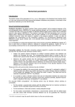
4.7.4
Example
Figure 4.4 illustrates a simplified example which was used for the modeling (in 2D) of two
buildings, the east façade of the tallest of which is covered with trees (presence of ”shade”
cells). Also noteworthy is the extension of the radiation mesh by ”horizon” cells to calculate the
radiative exchanges with the distant ground.
Accessibilité : EDF
Page 32/143
c
EDF
2012
EDF R&D
MFEE
User Manual for the SYRTHES code Version 4.2
Version 1.0
Figure 4.4: Modeling of two buildings and a wall of trees
Accessibilité : EDF
Page 33/143
c
EDF
2012
EDF R&D
MFEE
Accessibilité : EDF
User Manual for the SYRTHES code Version 4.2
Page 34/143
Version 1.0
c
EDF
2012
EDF R&D
MFEE
User Manual for the SYRTHES code Version 4.2
Version 1.0
Chapter 5
Heat and mass transfer: function
and specificities
Most of the thermal courses describe the 3 thermal transfer modes that are the conduction, convection and radiation. But, there is an another transfer mode, often forgotten : the enthalpic
transfer, connected to the transfers of mass. A fluid in movement transports its heat through
the space. This phenomenon is neither conduction, nor the convection, nor radiation. It is the
fourth phenomenon of thermal transfer.
In its most classical applications, the thermal analysis of buildings envelopes ignores totally
this phenomenon. The materials which constitute them are considered as purely conductive
and completely characterized by their thermal conductivity (even if we know that for many of
them, radiation in semi-transparent media contributes widely to the thermal exchange). At
the boundaries, on the interface between the components of envelope and the atmospheres, the
exchanges are represented as a simple mixe of convection and linearized infrared radiation.
Nevertheless, most of the materials which make up buildings’ envelopes are porous. The transfers
of mass can thus occur there. Besides, the most insulating materials are also the most porous,
thus potentially the most permeable. So, the maximum transfers of mass (high permeability)
correspond to the minimum transfers of heat (low thermal conductivity). From then on, for
the extremely successful components from standard thermal point of view, those for whom the
heat flux are the most low, it seems essential to examine more in detail the impact of the
mass transfers on the heat transfer. To reach there, it is necessary to handle the heat flux
question which allows to determine the main factors influencing the thermal performance of
these components. At this stage, it is necessary to use numerical taking into account heat and
mass transfers.
5.1
Physical model
We consider that the porous media is constituted by three phases :
• a solid phase, which is the skeleton of the material,
• a liquid phase constituted by pure water condensed in the pores of the material
• a gaseous phase which occupies the rest of the porous network.
syrthes supposes that the 3 phases are in equilibrium : they have the same temperature and
the 2 phases of water are in equilibrium.
Accessibilité : EDF
Page 35/143
c
EDF
2012
EDF R&D
MFEE
Version 1.0
User Manual for the SYRTHES code Version 4.2
The model programmed in syrthes used the 3 variables wich are :
• the temperature (T )
• the partial pressure of water vapor (Pv )
• the total pressure of the gas phase (Pt )
5.1.1
Equation de conservation de la masse d’eau :
dpv
ε
dT
v
βp − rεp
+
α
+
=
T
2
v T dt
∗
rv T dt
πv
πv∗ ~
L(T ) ~
pv
ρ l rv T ~
~ Kl ρl rv ln
∇.
∇T
+
+
K
∇p
+
ω
K
−
p
∇p
−
v
mv t
v p2
t
l pv
T
pt
psat (T )
t
5.1.2
Equation de conservation de la masse d’air sec :
dpv
αt (pt −pv )
−pv βp
ε dT
1
− prtas
+
−
+
ε
ρl
dt i +
hT ∗ρl T dt ras T
Kkrg
πv Mas ~
πv∗ pv Mas ~
∇. − pt Mv ∇pv + ρas ηt + p2 M
∇pt
t
5.1.3
ε dpt
ras T dt
=
v
Equation de conservation de la chaleur :
)
m ) βp pv +
ρs Cs + τv Cl − τv hp + ερv Cl + dL(T
+
ερ
C
−
(L(T
)
+
h
pas
dT
ρ l rv T
as dpv
pt αT
pv αT
ε
m
+ −τv hT + (L(T ) + h ) − ρl rv T + rv T + ρl
dt
dpt
−ε dt =
~ λ∗ ∇T
~ + (L(T ) + hm ) πv∗ ∇p
~ v + (L(T ) + hm ) ωmv Kt −
∇.
pt
Accessibilité : EDF
Page 36/143
πv∗ pv
p2t
~ t
∇p
εp v
rv T 2
+
pt βp
ρl
dT
dt
c
EDF
2012
EDF R&D
MFEE
5.2
User Manual for the SYRTHES code Version 4.2
Version 1.0
List of symbols
Symbole
ci
Cp
Cl
Cpas , Cpv
Cs
D
Dv
Das
e
f
G
g
~g
~gc
~gv
~gas
~v
G
~ as
G
H
h
has , hv ,hl
hm
hT
hP
h̄as
h̄c
h̄l
h̄v
h̄t
HR
K
Kt , Kl
krg , krl
L(T)
m
ṁ
mas
mv
ml
M
Mas
Mv
Accessibilité : EDF
Signification
Titre molaire du gaz i
Notation générique pour une chaleur massiqueà pression constante
Chaleur massique de l’eau liquide
Chaleur massique à pression constante de l’air sec et de la vapeur d’eau
Milieu poreux : Chaleur massique du matériau sec
Notation générique pour une diffusivité
Coefficient de diffusion de la vapeur d’eau dans l’air.
Coefficient de diffusion de l’air sec dans l’air.
Notation générique pour une épaisseur
Facteur de résistance à la diffusion dans un milieu poreux.
Notation générique pour une enthalpie libre.
Notation générique pour une enthalpie libre massique.
Notation générique pour une densité de flux
Densité de flux de chaleur dans le milieu poreux
Densité de flux de vapeur dans le milieu poreux
Densité de flux d’air sec dans le milieu poreux
Densité de flux de vapeur dansl’air.
Densité de flux d’air sec dansl’air.
Notation générique pour une enthalpie
Notation générique pour une enthalpie massique
Enthalpie massique de l’air sec,de la vapeur d’eau, de l’eau liquide
Chaleur de sorption de l’eau adsorbée
Dérivée partielle de hm par rapport à pv
Dérivée partielle de hm par rapport à T
Coefficient d’échange d’air sec
Coefficient d’échange de chaleur
Coefficient d’échange d’eau liquide
Coefficient d’échange de vapeur
Coefficient d’échange advectif du gaz
Humidité relative (pv /psat )
Perméabilité intrinsèque
Perméabilité au gaz, à l’eau liquide
Perméabilité relative au gaz, à l’eau liquide
Chaleur latente d’évaporation de l’eau
Notation générique pour une masse
Débit massique
Masse d’air sec
Masse de vapeur d’eau
Masse d’eau liquide
Rapport entre la masse molaire de l’air sec et celle de la vapeur d’eau
Masse molaire de l’air sec
Masse molaire de l’eau
Page 37/143
Unité
J/kg.K
J/kg.K
J/kg.K
J/(kg.K)
m2 /s
kg/m.s
kg/m.s
m
J
J/kg
W/m2
kg/(m2 s)
kg/(m2 s)
kg/(m2 s)
kg/(m2 s)
J
J/kg
J/kg
J/kg
J/kg.Pa
J/kg.K
kg/m2 .s
W/m2 .K
kg/m2 .s.P a
kg/m2 .s
kg/m2 .s.P a
m2
s
J/kg
kg
kg/s
kg
kg
kg
kg/mol
kg/mol
c
EDF
2012
EDF R&D
MFEE
User Manual for the SYRTHES code Version 4.2
Version 1.0
p
pas , pv
Pl
psat
pt
R
rv
ras
S
T
t
U
u
V
W
Notation générique d’une pression (Notation générique d’un périmètre)
Pression partielle d’air sec, de vapeur d’eau
Pression liquide
Pression de vapeur saturante
Pression totale de la phase gazeuse
Constante des gaz parfaits
Constante des gaz parfaits pour la vapeur d’eau (rv = R/Mv )
Constante des gaz parfaits pour l’air sec (ras = R/Mas )
Notation générique pour une surface
Notation générique pour une température
Notation générique pour le temps
Notation générique pourl’énergie interne
Notation générique pour une énergie interne massique
Notation générique pour un volume
Notation générique pour un travail.
Pa (m)
Pa
Pa
Pa
Pa
J/mol.K
J/kg.K
J/kg.K
m2
K
s
J
J/m3
m3
J
αT
∂τv
Pente de l’isotherme de sorption αt = ∂p
v
kg/m3 .P a
βP
ε
λ
λ∗
Λ
π
Π
πair
πapp
∗
πas
πv∗
µ
ηl
ηt
ωmi
%
ρas
ρl
ρs
ρv
ρt
τv
T
Dérivée partielle de l’isotherme de sorption par rapport à T
Porosité
Notation générique pour une conductivité thermique
Conductivité thermique du matériau humide
Chaleur totale de changement d’état de l’eau.Λ = L(T ) + hm
~ v)
Perméabilité à la vapeur d’eau (formule ~gv = −π ∇p
Notation générique pour une perméance (π/e)
~ v)
Perméabilité à la vapeur d’eau de l’air (formule ~gv = −πair ∇p
~ v)
Perméabilité à la vapeur d’eau apparente (formule ~gv = −πapp ∇p
∗ ∇(p
~ as /pt )
Coefficient de diffusion de l’air sec (formule ~gas,dif f = −πas
~ v /pt )
Coefficient de diffusion de la vapeur d’eau (formule ~gv,dif f = −πv∗ ∇(p
∗
Facteur de résistance à la vapeur d’eau ( µ∗ = ππa∗ )
v
Viscosité dynamique de l’eau liquide
Viscosité dynamique de la phase gazeuse
Titre massique du gaz i ( ρρti )
Notation générique pour une masse volumique
Masse volumique partielle de l’air sec
Masse volumique de l’eau liquide
Masse volumique du matériau sec.
Masse volumique partielle de la vapeur d’eau
Masse volumique totale d’un gaz
Taux d’humidité (masse d’eau par unité de volume de milieu poreux).
Accessibilité : EDF
Page 38/143
kg/m3 .K
W/m.K
W/m.K
J/kg
s
s/m
s
s
kg/(ms)
kg/(ms)
Pa.s
Pa.s
kg/m3
kg/m3
kg/m3
kg/m3
kg/m3
kg/m3
kg/m3
c
EDF
2012
EDF R&D
MFEE
User Manual for the SYRTHES code Version 4.2
Version 1.0
Chapter 6
Coupling with a thermal hydraulic
code
To understand multi-physical phenomena, syrthes can be used in association with a thermal
hydraulic code. This will enable a better comprehension of the boundary conditions for the fluid
or for the solid.
When doing a numerical simulation of a phenomenon, it is necessary to model and solve the
phenomenon inside the concerned domain and also to take into consideration the boundary
conditions at the interface. Most of the time, boundary conditions of a solid are relatively
unknown or are very difficult to understand. Taking into account the fluid domain can, in many
cases, eliminate this difficulty or, at least, reduce it significantly. For example, when a pipe is
thermally insulated, imposing an adiabatic (zero flux) condition on the exterior surface is quite
rigorous. On the contrary, if the material is thick or if a transient thermal evaluation is done,
imposing an adiabatic condition at the fluid/solid interface could lead to a significant error.
Figure 6.1: Modeling of a thermally insulated pipe
Another example of an application is the modeling of thermal transients.
The thermal interaction between fluid and solid is fundamental in cases of thermal shocks, which
are very frequent in industrial processes (nuclear hydraulics for example). Consider the case of
a thermal shock (significant and rapid increase of the fluid temperature) in a piping system.
Accessibilité : EDF
Page 39/143
c
EDF
2012
EDF R&D
MFEE
User Manual for the SYRTHES code Version 4.2
Version 1.0
The thermal inertia of the solid will lead to a gradual increase of temperature of the surface,
and inversely a partial cooling of the fluid. After a certain length, the impact of the shock may
be spread over the pipe and be considerably reduced. At the end of the pipe, the thermal load
is significantly lower which can become compatible with safety requirements, unlike the very
conservative attitude concerning a surface without thermal inertia.
Figure 6.2: Reduction of a thermal shock due to thermal inertia
In certain cases, interest in simulating a fluid/solid thermal coupling is in gaining knowledge
about the solid temperature field. Within this context, the simulation of thermal coupling with
the fluid provides better boundary conditions at the interface for the solid calculations.
This can be the case in the cooling process of a metallic object by water jets, air jets or by natural
convection. A classic approach consists of approximating the effect of the fluid by heat exchange
laws. Unfortunately, imposing these coefficients may lead to significant errors of measurement
where local parameters of the fluid temperature and the associated heat exchange coefficient are
difficult to determine.
Figure 6.3: Example: cooling of the internal baffle structure of a nuclear reactor
At the conclusion of the coupled calculations, the thermal results can be transferred to a mechanical code to determine the mechanical stresses originating from thermal phenomena. syrthes
can give the results in MED format [5] [6] (via a specific utility program avalaible in the
syrthes package: syrthes4med30), which can then be read, for example, by the mechanical
code Code Aster.
Accessibilité : EDF
Page 40/143
c
EDF
2012
EDF R&D
MFEE
User Manual for the SYRTHES code Version 4.2
Version 1.0
Chapter 7
General Environment
This chapter gives an outline of syrthes architecture and the tools that accompany it.
In the first paragraph, an overview is given. In the second paragraph, the organization of the
kernel of the code is described as well as its input and output files.
Figure 7.1: Flow chart of the syrthes program
Accessibilité : EDF
Page 41/143
c
EDF
2012
EDF R&D
MFEE
User Manual for the SYRTHES code Version 4.2
Version 1.0
Thermal radiation is presented as a syrthes module to differentiate the treatments of transfer
by conduction and by radiation (in a closed medium) during the use of the code. In this way, the
general functioning of the code is not overloaded. A unique keyword activates thermal radiation
in a closed medium.
Once this is activated, complementary data must be provided. On the contrary, if the module
is not activated, the keywords will simply not be read (note that it is not necessary to delete
the data file).
This approach is particularly flexible when evaluating the importance of radiation transfer in
a given problem: a calculation restricted only to conduction is directly possible from the calculation ”conduction+radiation” simply by deactivating the radiation calculation in the data
file.
7.1
Organization of the input data and the results
The general structure of the functioning of syrthesis presented in figure 7.2.
The parts indicated on the table in dashed lines are indicative of the radiation module.
Figure 7.2: Flow chart of syrthes functioning
The organization of the files is presented in the form seen in figure 7.3.
The complete description of these files is found in chapters 8, 12 and in appendix 13.
Accessibilité : EDF
Page 42/143
c
EDF
2012
EDF R&D
MFEE
User Manual for the SYRTHES code Version 4.2
Version 1.0
Figure 7.3: syrthes data and result files
7.1.1
Data files
The input files necessary for the syrthes code are the following:
• *.syr: a geometric file containing the non-structured mesh of the solid domain. This file
contains, among others, the list of elements, the coordinates of the nodes, the references for
the elements, etc. . . This file is in syrthesformat. Paragraph ?? examines possible tools
to generate such a file. In calculations with radiation, a second geometric file is necessary
to describe the radiating surface.
• syrthes data.syd: a file with diverse keywords (for the choice of options), the calculation parameters, the numerical criteria associated with the resolution, the physical
conditions and the boundary conditions. Even if the name of this file is traditionally
syrthes data.syd, it is not imposed and can be changed as necessary.
• User source files (user.c,user cond.c,user ray.c, user hmt.c) which are optional but
useful to define complex conditions. Chapter 12 describes these functions.
Accessibilité : EDF
Page 43/143
c
EDF
2012
EDF R&D
MFEE
7.1.2
User Manual for the SYRTHES code Version 4.2
Version 1.0
Result files
syrthes generates a certain number of result files relative to the options chosen for the simulation. All the names of the file results have the same prefix and are distinguished by their
extension:
• .res: result file containing the principle variables of the calculation in each node of the
mesh. It is the temperature for a calculation of conduction/radiation. If the model of heat
and mass transfer is activated, they are the temperature, the vapor pressure and the total
pressure.
• .rdt: transient: similar to the previous result file but containing the results in several
time steps defined by the user.
• .his: history file: for tracking the evolution of the temperature over time (and also the
vapor pressure and the total pressure) on a limited number of points defined by the user
(probes).
• .mnx: minimum and maximum file: at each time step, syrthes calculates the minimum and maximum of a certain number of variables. These values are saved in columns
in the file.
• .flu: heat balance file: if the user requests it in the data file, it is possible to calculate
the surfacic heat balance and/or the volumetric heat balance at each time step. The values
are displayed in the listing file but also in this file which can later be used to trace curves.
• .add: additional file: This file is optional. It enables the user to save certain variables or
parameters in the file which can then be visualized in the post-processor. The structure of
this file is identical to that of a traditional result file. Parameters calculated on the mesh
nodes as well as parameters calculated on the elements can be saved here.
Thermal radiation in the calculations does not generate results in themselves because they are
interpreted by the modification of the temperature field in the solid. It is thus the traditional
syrthes result files which handle the coupling of conduction + radiation phenomena.
Nevertheless, it is interesting to have access to certain parameters directly linked to radiation.
Thus, it is possible to request the code to generate certain results directly on the radiation mesh.
As for solids, three files are available:
• rad.res: a result file which contains the temperature and the radiation flux per band
• rad.rdt: a chronological file which contains the temperature and the radiation flux per
band but in diverse time steps
Remark: in radiation, the discretization used is type P0 ; meaning that the parameters are constant per cell.
Accessibilité : EDF
Page 44/143
c
EDF
2012
EDF R&D
MFEE
7.1.3
User Manual for the SYRTHES code Version 4.2
Version 1.0
Storage/Memory file for view factors
This file (mesh.fdf) is only used in calculations for the coupling of conduction + radiation. It
is not directly exploitable by the user but stores information very expensive to calculate. In
the initial phase, it is necessary to calculate the geometric parameters quantities which are the
view factors, generally considered as being costly with a large number of mesh cells. The total
number of view factors is n(n − 1)/2 if n is the number of independent cells.
syrthes includes an option to save the parameters in the file which avoids the recalculation
of the parameters for subsequent calculations. Indeed, these parameters are purely geometrical
and remain constant if the geometry does not change.
7.1.4
Coupling syrthes with a thermal hydraulic code
In the case of coupling syrthes with a CFD code, the file organization remains unchanged. The
files relative to the fluid code are simply added to the syrthes directory. A specific script will
simultaneously launch both the fluid and solid applications using MPI [7] (see chapter 6).
7.2
Creating a mesh for syrthes
As for any industrial calculations, the large volume of data for the calculation absolutely necessitates the use of eficient pre- and post- processors.
The mesh of finite elements of the solid domain can be done with any mesh generator: the
structures of the data issued from the mesher must be compatible with those accepted by
syrthes.
Currently, syrthes includes a conversion tool convert2syrthes4 which automatically recognizes files formatted in gambit, gmsh, Ideas-MS, Salomé, simail. convert2syrthes4: conversion of a mesh file to syrthes format convert2syrthes4 -m geo.xxx [-r geo.syr]
. geo.xxx: name of mesh file (.neu, .msh, .unv, .med, .des)
. geo.syr: name of mesh file converted to syrthes format (if the name is not provided, it will
automatically be named geo.syr).
The use of all other mesh generators is possible on the condition that they are compatible with
the syrthes format (see the format of files in Appendix A).
7.3
Visualize syrthes results
Whatever the option retained, syrthes always provides a result file containing the value of
temperature at each mesh node.
Utility programs transform these results into syrthes format in a data base compatible with
diverse post-processors.
The format of syrthes result files are given in Appendix A.
Accessibilité : EDF
Page 45/143
c
EDF
2012
EDF R&D
MFEE
7.3.1
User Manual for the SYRTHES code Version 4.2
Version 1.0
Conversion of syrthes results to Ensightformat
syrthes4ensight: transformation of a syrthes file to an Ensight data base formatted enquotecase.
use: syrthes4ensight -m geo.syr
-r resu1.res
-o fich ensight
. geo.syr: name of syrthesgeometric file,
. resu1.res: name of syrthesresult file. This file can be either the result file (.res) containing
only one time step or the transient file (.rdt) which will treat n time steps.
. fich ensight: name of the file in Ensightformat
Note that this file format can then be read by Ensight and paraview paraview.
7.3.2
Conversion of results to med format
syrthes4med30: transformation of a syrthes file to a med data base med [9].
Use: syrthes4tomed30 -m geo.syr -r resu1.res -o fichier.med
. geo.syr: name of syrthes geometric file
. resu1.res: name of syrthes result file
. fichier.med: name of file containing the mesh and results in med format
Accessibilité : EDF
Page 46/143
c
EDF
2012
EDF R&D
MFEE
User Manual for the SYRTHES code Version 4.2
Version 1.0
Chapter 8
Data files relative to SYRTHES
To do a calculation, syrthes requires at least a parameter file, where the case and the numerical
choices can be precisely defined, and a geometric file for the description of the calculation domain.
8.1
Geometric Files
8.1.1
Conduction mesh
This file is mandatory. This file contains the mesh of the solid domain as well as diverse references
applied on the nodes, the boundary edges in 2D or faces in 3D of the mesh.
The solid mesh being unstructured, syrthes requires necessary information: a table of node
coordinates, the connectivity of the volumetric mesh and the connectivity of the boundary mesh.
The mesh must be composed exclusively of the following:
• 3-node triangles in two dimensions (triangles with straight sides), and 2-node edges for the
boundary
• 4-node tetrahedrons in three dimensions (tetrahedrons with planar surfaces), and 3-node
triangle for the boundary
8.1.2
Radiation mesh
When the thermal radiation calculation is activated, a second mesh must be provided to syrthes which
is also unstructured.
syrthes requires necessary information: a table of node coordinates and the connectivity of the
mesh with references of the elements.
The surfacic mesh is composed exclusively of the following:
• 2-node segments in two dimensions
• 3-node triangles in three dimensions
Note that the conduction and radiation meshes are totally independent and that it is absolutely
not necessary that they are coincident (conformal) (but they can be as well).
Accessibilité : EDF
Page 47/143
c
EDF
2012
EDF R&D
MFEE
8.1.3
User Manual for the SYRTHES code Version 4.2
Version 1.0
Formats of the mesh files
syrthes 4 only authorizes one type of mesh: the syrthes format. This format is described the
appendix.
To obtain a mesh in this format, syrthes includes a file conversion tool.
This utility convert2syrthes accepts the input from the following formats:
• simail mesh generator files (extension .des),
• Ideas-MS mesh generator files (extension .unv),
• Salomé mesh generator files in med format (extension .med),
• gmsh mesh generator files (extension .msh),
• gambit mesh generator files (extension .neu),
The identification of the file format is made by the extension which is given to the name of the
geometric file. This extension is thus imposed and mandatory.
8.2
Parameter files
This file contains all the user parameters to do a calculation. The following chapter is entirely
devoted to it. It is generally named syrthes data.syd.
8.3
Standard weather data file
For calculations in which meteorological conditions must be input, it is possible to provide
syrthes with a complementary weather file.
The name of this file is provided by the syrthes parameter filesyrthes data.syd.
FICHIER METEO=If the name of the file is provided, it will be automatically read when the
calculation starts running and the information read can be used in the user functions of the
filesuser.c, user cond.c, user hmt.c and user ray.c.
8.3.1
Contents of the weather data file
In this file, the data is provided in columns. The first line is particular: it indicates the number
of columns in the file.
The weather file is read line by line, regardless of the number of columns.
Generally, each line corresponds to an instant and on the same line different variables of this
instant are found.
Below is an example of a weather file:
3
0
300
20
22
Accessibilité : EDF
5.1
5.5
Page 48/143
c
EDF
2012
EDF R&D
MFEE
600
900
1200
24
23
21
User Manual for the SYRTHES code Version 4.2
Version 1.0
5.3
6.2
5.8
In this example, the first line indicates that each line is composed of three variables. After that,
on each line is given: the time in seconds, the exterior temperature and the wind velocity.
After having read the file, the data are stored in the meteo structure of the Meteo type. The
number of lines in the chart is stored in the variable meteo.nelem.
The following table summarizes the content of the weather file and provides the variables in
which information is stored in syrthes.
This data can then be used in the different user functions.
8.3.2
Example of use
An example of the use of data provided in a weather data file is described below (on the basis of
the example presented above). This represents only a fraction of the user function user limfso
available in the file user cond.c.
For this example, a condition for heat exchange on the boundary of the domain is imposed. The
heat exchange coefficient is set at 10 W/(m2 K), the exterior temperature is provided by the
weather file.
In the data file syrthes data.syd, a heat exchange condition is imposed on the boundary of
reference 1:
CLIM_T_PROG=
COEF_ECH
1
The function user limfso of the file user.c is programmed in the following way:
/* Heat Exchange Condition */
/* ----------------------- */
if (mescoeffech)
{
/* Searching the time step */
if (tempss <= meteo.var[0][0])
num=0;
else if (tempss >= meteo.var[0][meteo.nelem-1])
num=meteo.nelem-1;
else
{
num=1;
while (tempss>meteo.var[0][num]) num++;
num--;
}
Accessibilité : EDF
Page 49/143
c
EDF
2012
EDF R&D
MFEE
User Manual for the SYRTHES code Version 4.2
/* For each node of each heat exchange boundary
for (j=0;j<echang.ndmat;j++)
for (i=0;i<echang.nelem;i++)
{
nr=maillnodeus.nrefe[echang.numf[i]]; /*
if (nr==1){
/*
echang.val1[j][i]=meteo.var[1][num];
echang.val2[j][i]=10;
}
}
Version 1.0
element */
boundary element reference
*/
if the reference is 1
*/
/* Temperature found in the file */
/* Heat exchange coefficient
*/
}
8.4
User data files
Certain calculations can necessitate the use of particular data originating, for example, from
measurements or from calculations done in other disciplines having an impact on the thermal
modeling.
In this case, syrthes includes a pre-programmed function to read data from a file provided by
the user regardless of the format. The user function can be modified according to the file content.
The file will be read by the function user read myfile of the file user.c.
The read data will be stored in the structure myfile. The following fields are also included in
this structure:
• myfile.actif: activation of the reading of a personal file
• myfile.nbvar: number of variables to read
• myfile.nelem: number of values per variable
• myfile.var[myfile.nbvar][myfile.nelem]: values of the variables
After having input the number of variables and the number of values per variable to read in
section 1 of the function, the reading of the file is then programmed in section 3 in the file
format.
Accessibilité : EDF
Page 50/143
c
EDF
2012
EDF R&D
MFEE
User Manual for the SYRTHES code Version 4.2
Version 1.0
Chapter 9
Interpreted functions
As seen in previous chapters, syrthes can handle variable physical characteristics (boundary
conditions, physical properties,. . . ). In a great number of cases the variations of these parameters are expressed in the form of functions dependent on space, time and temperature.
To facilitate the definition of these variation functions and to limit the programming of the user
functions to very specific and complex configurations, syrthes defines these functions directly
in the data file syrthes.data.syd.
9.1
What can be defined with the interpreted functions?
syrthes accepts interpreted functions for the following parameters:
• Initial conditions of temperature, vapor pressure and total pressure
– keyword CINI T FCT=
– keyword CINI PV FCT=
– keyword CINI PT FCT=
• Temperature boundary conditions
– Heat exchange condition (value of the exterior temperature and of the heat exchange
coefficient)
keyword CLIM T FCT=
– Dirichlet Condition (value of the imposed temperature)
keyword CLIM T FCT=
– Flux Condition (value of the surface flux)
keyword CLIM T FCT=
• Physical properties
– for isotropic materials
keyword CPHY MAT ISO FCT=
Accessibilité : EDF
Page 51/143
c
EDF
2012
EDF R&D
MFEE
User Manual for the SYRTHES code Version 4.2
Version 1.0
– for orthotropic materials
keyword CPHY MAT ORTHO 2D FCT=
keyword CPHY MAT ORTHO 3D FCT=
– for anisotropic materials
keyword CPHY MAT ANISO 2D FCT=
keyword CPHY MAT ANISO 3D FCT=
• Volumetric flux on temperature, vapor pressure and total pressure
keyword CVOL T FCT=
keyword CVOL PV FCT=
keyword CVOL PT FCT=
9.2
How to define a function?
A function is an expression which can use all the mathematical symbols and functions known
in programming language C. It cannot include the space character which is considered as a
delimiter. The variables which can be present in the expression are the following (upper and
lower cases must be respected!):
• tt: physical time (in seconds)
• T: temperature (in degrees C)
• x,y,z (z is only allowable in 3 dimensions): the coordinates of the node or of the center of
a cell (in meters)
Example: definition of properties of an isotropic material where the volumetric mass and the
heat capacity are constant but where the conductivity is defined by an interpreted function.
CPHY_MAT_ISO_FCT=
9.3
7700
460.
0.07223+0.005211*tt-1.197e-5*tt*tt
24 23 26
Interpreted functions in syrthes
Once the functions have been defined in the user data file syrthes.data, a specific pre-processor
(ppfonc syrthes) interprets and generates the corresponding C functions.
Generally, this phase is hidden to the user because it is integrated in the script/command to
run syrthes. The command for manual use of the pre-processor is provided:
ppfonc_syrthes syrthes_data.syd
Once the code has finished being executed, the file (util fct.c)is made available which will be
taken into account at the moment of the execution of the code.
Accessibilité : EDF
Page 52/143
c
EDF
2012
EDF R&D
MFEE
User Manual for the SYRTHES code Version 4.2
Version 1.0
Chapter 10
Parameter file
Generally, the syrthes parameter file is named syrthes data.syd, which is not imposed and can
be changed whenever desired. However, for convience and clarity, this appellation will be used
in this document.
This file is made up of keywords with default values which must be input.
10.1
Genaralities concerning the data file syrthes data.syd
This file is input through the user interface syrthes.gui.
By following the different interface rubrics, the input data are defined. All data are stored in
the file syrthes data.syd which will be read by syrthes.
The syrthes data.syd file is a text file composed of keywords. Even if it is generally automatically filled by the syrthes.gui interface, it is nevertheless possible to input in it by using
a simple ”text editor”. This is interesting in particular cases, for example, parametric calculations which may require a large number of calculations by modifiying only some of the input
parameters. The sequence of the calculations can managed automatically by running the userś
own script.
For this reason, the description of input data via the user interface is described in this chapter,
but by specifying the corresponding keyword in the file syrthes data.syd.
Below are all the notations useful for the functioning of the syrthes data.syd file:
• The order of keywords is random,
• The keywords, nevertheless, are grouped by theme and generally preserve the proposed
order to maintain a certain logic in the file,
• syrthes then reads the file sequentially: if a keyword appears several times it is the last
value read which will be used for the calculation,
• For a given keyword, all the parameters must be provided on the same line,
• All lines starting with the character ”/” are comments,
• Keywords that are not used can be deleted from the file
Accessibilité : EDF
Page 53/143
c
EDF
2012
EDF R&D
MFEE
User Manual for the SYRTHES code Version 4.2
Version 1.0
• Keywords relative to radiation (ie. keywords in the paragraph Data for Radiation ”DONNEES POUR LE RAYONNEMENT” are not read unless the keyword ”PRISE EN COMPTE
DU RAYONNEMENT CONFINE=” was previously positioned to ”oui”),
• Keywords relative to humidity transfer (ie. key words in the paragraph ”DONNEES
COMPLEMENTAIRES POUR LES TRANSFERTS COUPLES” Complementary data for
coupled transfers are not read unless the keyword ”MODELISATION DES TRANSFERTS
D HUMIDITE=” was previously positioned to ”oui”.
• Most of the parameters have default values.
Once placed in the directory corresponding to the case being studied, syrthes graphic interface
will be launched by typing:
syrthes.gui
10.2
Genaralities concerning the tables in the syrthes.gui interface
For the functioning of syrthes several types of variables must be read. It is possible to distinguish a part of the parameters by simply defining a value. It is possible, for example, to cite the
definition of the value of the time step: syrthes accepts a real value which will define the latter.
But there are also more complex data such as the initial conditions, boundary conditions and
physical conditions. Input data in the code, a list of conditions must be provided. In these cases,
syrthes.gui will propose a definition of the values in a table. Figure 10.1 shows an example of
such.
Figure 10.1: syrthes.gui - Window: Example of a table
The definition of initial conditions will now be considered.
Accessibilité : EDF
Page 54/143
c
EDF
2012
EDF R&D
MFEE
User Manual for the SYRTHES code Version 4.2
Version 1.0
The mesh was planned in consequence and contains different zones where the elements have
different references.
Three types of conditions are possible:
• Constant: the value of the condition is constant, it is a real value. In this case, the value
of the condition, and the list of references of the elements of the mesh where it is applied,
must be provided and a comment can be added if desired.
• Function: the value of the condition can be expressed in the form of an interface function
”interprétée” and can be written relative to the variables t (time), T (temperature), x,
y, z (spatial coordinates). In this case, it is necessary to provide the function which is
expressed by using exclusively the variables cited t, T , x, y, z (respect the upper and lower
cases) and the list of references of elements of the mesh where it is applied. A comment
can be added if necessary.
• Program: the value of the condition is complex (interpolation in a file for example) and
it will be directly programmed in the user source files. The references of elements of the
mesh where it is applied must be provided, and a comment can be added if desired.
Figure shows an example:
Figure 10.2: syrthes.gui - Window: Example where different types of conditions are used
Non-utilization of certain conditions
By default, all the conditions defined are active and will be taken into consideration in the calculation. This is reflected in the window where the beginning of each line is checked (presence
of an X).
Accessibilité : EDF
Page 55/143
c
EDF
2012
EDF R&D
MFEE
User Manual for the SYRTHES code Version 4.2
Version 1.0
In certain cases, certain conditions may not want to be taken into consideration without deleting
√
them from the file (to reactivate them later). In this case, the must simply be deactivated at
the beginning of the line: the condition will be written in the user comments section of the data
file and will not be taken into consideration for the calculation.
An example is seen in figure 10.3: for reference 2; the initial temperature of 28◦ C was deactivated
and recorded in the above line as 23◦ C(reference 2 is seen in the comments as ”low temperature
zone”).
Figure 10.3: syrthes.gui - Window: example with partial deactivation of conditions
The input of data will now be described by using the syrthes.guiinterface windows.
Accessibilité : EDF
Page 56/143
c
EDF
2012
EDF R&D
MFEE
10.3
User Manual for the SYRTHES code Version 4.2
Version 1.0
Home window
The home window appears at the startup of the interface:
Figure 10.4: syrthes.gui - Window: Home
The following data must be provided:
B Case title
Description
Keyword
Value
Default
It is possible to entitle the study here.
titre etude=
String of characters
—
B User description of the case
Description It is possible to add a comment for the description of the study here
Keyword
non-applicable
Value
—
Default
—
B Dimension of the problem
Description Definition of the dimension of the study which can be in 3 dimensions
(3D), 2 dimensions
Keyword
dimension du probleme=
Value
2d cart or 2d axi ox or 2d axi oy or 3d
Default
3d
Finally, it is possible to activate the different physical models in syrthes:
Accessibilité : EDF
Page 57/143
c
EDF
2012
EDF R&D
MFEE
User Manual for the SYRTHES code Version 4.2
Version 1.0
B Thermal radiation
Description Activation of the thermal radiation model
Keyword
prise en compte du rayonnement confine=
Value
oui or non
Default
non
B Humidity
Description
Keyword
Value
Default
10.4
Activation of of transfers coupled with mass and temperature. Two
models are available: models with 2 equations (temperature and vapor
pressure) and models with 3 equations (temperature, vapor pressure and
total pressure)
modelisation des transferts d humidite=
0, 2 or 3
0
Control of window
The adjustment of the parameters for the calculation pilot can be done in this window.
It has two tabs. The first (Time managment) is for the management of time, and the second
(Solver information) is to control iterative solver parameters.
10.4.1
Time management tab
In general it is the management of time that is dealt with here.
syrthes is, above all, based on an unsteady algorithm. A convergence of the usteady algorithm
is used for research in a steady state.
In numerous cases, the calculation is not made in only one run. A first calculation is done,
the results are analyzed and a new calculation is launched taking as the initial parameters the
results from the first calculation. It is a sequence of calculations.
In other cases, a system usually in a steady state which is suddenly subjected to a transient
might need to be studied. In this case, the steady state will be calculated first before the starting
of the transient. In this case, a sequence of calculations will be executed but it will be equally
possible to ”reset” the physical time to start the transient to t = 0 for example.
B Restart calculation
Description A sequence of calculations, it is necessary to later provide the result file
of the first calculation as the input data.
Keyword
suite de calcul=
Value
oui or non
Default
non
Accessibilité : EDF
Page 58/143
c
EDF
2012
EDF R&D
MFEE
User Manual for the SYRTHES code Version 4.2
Version 1.0
B Setting a new restart time
Description In the case of a sequence of calculations, it is possible to redefine the
physical start time (adjustment for example)
Keyword
suite: nouveau temps initial=
Value
If real < 0: no modification, time restart is done according to time
indicated on the next file
Value
If real > 0: the physical time is reset to this value
Default
-1
Management of time and of time steps.
The number of time steps is indicated in a global way on the totality of the calculation. Thus,
if 150 time steps have been done during the first calculation and that 200 more are needed
during subsequent calculations, the number of time steps to indicate will be 350. In this way,
the chronology of calculations can be conserved and the management of the sequence will be
easier.
Three time steps options are possible:
• constant: the same time step will be used throughout the calculation, only one value
needs to be provided to the code.
• automatic: the time step is calculated automatically by the syrthes function of the
gradient of the temperature. In this case, an initial time step needs to be input and the
maximum of temperature variation authorized between two successive time steps. Finally,
a maximum value of the time step is requested in order to set it when the convergence is
attained.
• by blocks: several constant time steps can be defined during the calculation. For example,
the first ten time steps are of 1.5s, the next 30 time steps are of 0.5s, and the 100 subsequent
time steps are at 1s.
B Global number of time steps
Description Number of time steps at which the code will stop
Keyword
nombre de pas de temps solides=
Value
integer > 0
Default
—
B Time step: Constant
B Time step (in seconds)
Description Choice of one constant time step
Keyword
pas de temps solide=
Value
real > 0
Default
—
Accessibilité : EDF
Page 59/143
c
EDF
2012
EDF R&D
MFEE
User Manual for the SYRTHES code Version 4.2
Version 1.0
B Time step: Automatic
Description Choice of one automatic time step, based on the temperature gradient
Keyword
pas de temps solide=Solid time step
Value
—
Keyword
pas de temps automatique=
Value
gradient T max (real > 0), max time step (real > 0)
Default
——
B Time step: By blocks
Description Choice of a constant time step per block
Keyword
pas de temps multiples=
Value
Iteration value (whole > 0), max time step (real > 0)
Default
——
10.4.2
Solver information tab
The equation of heat in a solid is resolved with an iterative method of a preconditioned conjugated gradient type.
The precision of the resolution can be adjusted. A compromise between the desired precision
and the calculation time necessary to resolve it is found with two values designed for this effect.
It is necessary, here, to point out a technical point: the stop test of the iterative method employed is based on three criteria:
• the maximum number of iterations given,
• a criterion of absolute convergence (kAx − bk < εabs ),
< εrel )where xn is the result of the resolution
• a criterion of relative convergence ( kAx−bkk
kxn k
to the preceding time step.xs.
The algorithm stops:
• when the number of maximum iterations is attained,
• when the two criteria of convergence are respected.
In this way, the solver can be completed piloted:
• to request a very exact precision: by imposing a very strict criterion of absolute convergence
and a sufficiently large number of iterations,
• to request a less precise and/or to limit the numberof iterations.
When the resolution of the coupled transfers is activated, similar criteria are used for the vapor
pressure and total pressure variables.
Accessibilité : EDF
Page 60/143
c
EDF
2012
EDF R&D
MFEE
User Manual for the SYRTHES code Version 4.2
Version 1.0
B Solver precision
Description Precision requested to the iterative solver of the linear system for the
resolution of conduction
Keyword
nombre iterations solveur temperature=
Value
integer > 0
Default
100
Keyword
nombre iterations solveur pression de vapeur=
Value
integer > 0
Default
100
Keyword
nombre iterations solveur pression totale=
Value
integer > 0
Default
100
B Maximum number of iterations
Description maximum number of iterations authorized for the iterative solver of the
linear system for the resolution of conduction
Keyword
precision pour le solveur temperature=
Value
real > 0
Default
10−5
Keyword
precision pour le solveur pression de vapeur=
Value
real > 0
Default
10−5
Keyword
precision pour le solveur pression totale=
Value
real > 0
Default
10−5
10.5
Window: File Names
This window provides the names of the syrthes data and result files. The first frame is dedicated
to the data files.
• Conduction mesh: It is necessary to input at least the name of the mesh for the
resolution of the conduction. Note that if the mesh file is not in syrthesformat, the
syrthes.gui interface will automatically use the converter of format1 to have a mesh file
in syrthesformat1 .
• Radiation mesh: In the case where the thermal radiation is activated in the principle
window, the name of the radiation mesh must also be input.
• Restart File: In the case of sequential calculations, it is necessary to input the name of
the results file from which the new calculation can be launched. Only the prefix must be
given.
1
7.2
Accessibilité : EDF
Page 61/143
c
EDF
2012
EDF R&D
MFEE
User Manual for the SYRTHES code Version 4.2
Version 1.0
• Weather data: Optionally, a weather data file can be input including values that can be
used in the boundary conditions for example.
Figure 10.5: syrthes.gui - Window: File Names
The second frame is dedicated to the Results Names files.
• Results names prefix: the prefixes of the result files are defined here. All the general
files per code will take this prefix and can then be distinguished by the extensions.
Warning: if an existing prefix name is input, the former results will be deleted
by the new calculation.
Accessibilité : EDF
Page 62/143
c
EDF
2012
EDF R&D
MFEE
User Manual for the SYRTHES code Version 4.2
Version 1.0
B Conduction mesh
Description Name of the conduction mesh
Keyword
maillage conduction=
Value
String of characters without spaces
Default
—
B Radiation mesh
Description Name of the radiation mesh file
Keyword
maillage rayonnement=
Value
String of characters without spaces
Default
—
B Restart file
Description Name of the file for sequencial calculations
Keyword
prefixe du resultat precedent pour suite de calcul=
Value
String of characters without spaces
Default
—
B Weather data
Description Name of weather data file
Keyword
fichier meteo=
Value
String of characters without spaces
Default
—
B Results names prefix
Description Prefixe that will be used for all the results files
Keyword
prefixe des fichiers resultats=
Value
String of characters without spaces
Default
—
Accessibilité : EDF
Page 63/143
c
EDF
2012
EDF R&D
MFEE
User Manual for the SYRTHES code Version 4.2
10.6
Parameters for conduction
10.6.1
Window: Initial conditions
Version 1.0
Definition of the initial conditions: The initial temperature of all the nodes of the mesh must
be input.
If, and only if, the initialization is identical in the entire domaine (either a uniform temperature,
the same function throughout, or an initial condition programmed for the entire domain), the
list of references of the elements concerned can be reduced to ”-1” meaning ”all the elements”.
Figure 10.6: syrthes.gui - Window Conduction - Initial conditions
B Initial conditions
Description Initial temperature in ◦ C
Keyword
cini t= temperature references
Value
Real
Default
T = 20
Keyword
cini t fct= temperature references
Value
fonction T(x,y,z,t,T)
Default
T = 20
Keyword
cini t prog= references
Value
user.c(user cini) to program
Default
T = 20
10.6.2
Window: Boundary conditions
Definition of the boundary conditions: This window includes 5 tabs which define the boundary
conditions according to their type.
Accessibilité : EDF
Page 64/143
c
EDF
2012
EDF R&D
MFEE
User Manual for the SYRTHES code Version 4.2
Version 1.0
For each boundary condition, the list of references of the boundary faces concerned by this
condition is provided.
Remark 1: all boundary faces for which no boundary condition is specified will automatically be
considered as adiabatic (zero flux).
Remark 2: for the resolution of the conduction in syrthes an adiabatic (zero flux) condition
of (or of symmetry) is not required to be explicitly imposed. This part of the domain boundary
should simply be left without a boundary condition.
10.6.2.1
Heat exchange tab
Heat exchange boundary condition: An exterior temperature (in ◦ C) and a heat exchange
coefficient (W/m2 /◦ C) must be input.
Figure 10.7: syrthes.gui - Window: Boundary conditions - Heat Exchange
B Boundary conditions - Exchange
Description Boundary condition of Heat Exchange
Keyword
clim t= coef ech T h references
Value
Real, Real
Default
T=20, h=0
Keyword
clim t fct= coef ech T h references
Value
2 functions T (x, y, z, t, T ) et h(x, y, z, t, T )
Default
T=20, h=0
Keyword
clim t prog= coef ech References
Value
user.c(user limfso) to program
Default
T=20, h=0
Accessibilité : EDF
Page 65/143
c
EDF
2012
EDF R&D
MFEE
10.6.2.2
User Manual for the SYRTHES code Version 4.2
Version 1.0
Flux tab
Flux boundary condition: The flux in W/m2 must be input.
Figure 10.8: syrthes.gui - Window: Boundary conditions - Flux
B Boundary conditions - Flux
Description Boundary condition of type Flux
Keyword
clim t= flux Flux references
Value
Real
Default
ϕ=0
Keyword
clim t fct= flux Flux references
Value
function varphi(x, y, z, t, T )
Default
ϕ=0
Keyword
clim t prog= flux references
Value
user.c(user limfso) to program
Default
ϕ=0
Accessibilité : EDF
Page 66/143
c
EDF
2012
EDF R&D
MFEE
10.6.2.3
User Manual for the SYRTHES code Version 4.2
Version 1.0
Dirichlet tab
Dirichlet boundary condition: An imposed temperature in ◦ Cmust be input here.
Figure 10.9: syrthes.gui - Window: Boundary conditions - Dirichlet
B Boundary conditions - Dirichlet
Description Boundary condition of type imposed temperature
Keyword
clim t= dirichlet temperature references
Value
Real
Default
T =0
Keyword
clim t fct= dirichlet T (x, y, z, t, T ) References
Value
function
Default
T =0
Keyword
Clim t prog= dirichlet references
Value
user.c(user limfso) to program
Default
T =0
Accessibilité : EDF
Page 67/143
c
EDF
2012
EDF R&D
MFEE
10.6.2.4
User Manual for the SYRTHES code Version 4.2
Version 1.0
Contact resistance tab
Contact resistance boundary condition: The value of the contact resistance must be input here
in W/m2 /◦ C and the references of the two groups of faces between which the contact resistance
will be applied. Note that in the data file syrthes.data the two reference groups are separated
by ”-1”.
Figure 10.10: syrthes.gui - Window: Boundary conditions - Contact resistance
B Boundary conditions - Contact resistance
Description Boundary condition of type imposed temperature
Keyword
clim t= res contact g ref groupe 1 -1 ref groupe 2
Value
Real
Default
g=0
Keyword
clim t fct= res contact g(x, y, z, t, T ) Resistance ref groupe 1 -1
ref groupe 2
Value
fonction g(x, y, z, t, T )
Default
g=0
Keyword
clim t prog= res contact ref groupe 1 -1 ref groupe 2
Value
user.c(user limfso) to program
Default
g=0
Accessibilité : EDF
Page 68/143
c
EDF
2012
EDF R&D
MFEE
10.6.2.5
User Manual for the SYRTHES code Version 4.2
Version 1.0
Infinite radiation tab
Infinite radiation boundary condition: The value of the emissivity of the surface and the infinite
temperature (◦ C) must be input here.
Figure 10.11: syrthes.gui - Window: Boundary conditions - Infinite radiation
B Boundary conditions - Infinite radiation
Description Boundary condition of type Infinite radiation
Keyword
clim t= ray infini ε T∞ References
Value
Real∈ [0, 1],real
Default
ε = 0, T=20
Keyword
clim t fct= ray infini ε T∞ References
Value
2 function f (x, y, z, t, T )
Default
ε = 0, T=20
Keyword
clim t prog= ray infini references
Value
user.c(user limfso) to program
Default
ε = 0, T=20
10.6.3
Physical properties window
Definition of the physical properties of materials:
This window includes three tabs which define isotropic, orthotropic and anisotropic materials
within the same domain of calculation.
If, and only if, the domain is only composed of one single material, the list of references of the
elements concerned can be reduced to ”-1”. If not, for each material, the list of references of
elements concerned by this condition will be provided.
Accessibilité : EDF
Page 69/143
c
EDF
2012
EDF R&D
MFEE
10.6.3.1
User Manual for the SYRTHES code Version 4.2
Version 1.0
Isotropic tab
Definition of materials with isotropic behavior: the thermal conductivity will thus be defined by
a scalar (possibly variable in time and space) on the elements.
Figure 10.12: syrthes.gui - Window: Physical properties - Isotropic
Isotropic solids are defined by:
. the volumetric mass ρ (kg/m3 )
. the heat capacity Cp (J/kg K)
. the thermal conductivity k (W/mK)
B Physical properties - Isotropic - Type=Constant
Description Isotropic materials with properties defined by a constant
Keyword
cphy mat iso= ρ Cp k references
Value
3 real > 0
Default
7700 460 25
B Physical properties - Isotropic - Type=Function
Description Isotropic materials with properties defined by a function
Keyword
cphy mat iso fct= ρ Cp k references
Value
3 functions f (x, y, z, t, T )
Default
7700 460 25
B Physical properties - Isotropic - Type=Program
Description Isotropic materials with programmed properties
Keyword
cphy mat iso prog= references
Value
—
Default
7700 460 25
10.6.3.2
Orthotropic tab
Definition of materials with orthotropic behavior: the thermal conductivity will thus be defined by a diagonal matrix (the terms of which can vary in time and space) on the elements.
Orthotropic solids are defined by:
Accessibilité : EDF
Page 70/143
c
EDF
2012
EDF R&D
MFEE
User Manual for the SYRTHES code Version 4.2
Version 1.0
Figure 10.13: syrthes.gui - Window Physical properties - Orthotropic
Orthotropic solids are defined by:
. volumetric mass ρ (kg/m3 )
. heat capacity Cp (J/kg K)
. thermal conductivity (W/mK) It is necessary to give 2 or 3 values (respectively in 2D and
3D): The conductivity following the direction x, y and possibly z.
B Physical properties - Orthotropic - Type=Constant
Description
Orthotropic materials with properties defined by a constant
Keyword 2D cphy mat ortho 2d= ρ Cp kx ky references
Keyword 3D cphy mat ortho 3d= ρ Cp kx ky kz references
Value
4 or 5 real > 0
Default
rho = 7700 Cp = 460 kx = 25 ky = 25 kz = 25
B Physical properties - Orthotropic - Type=Function
Description
Orthotropic materials with properties defined by a function
Keyword 2D cphy mat ortho 2d fct= ρ Cp kx ky references
Keyword 3D cphy mat ortho 3d fct= ρ Cp kx ky kz references
Value
4 or 5 functions f (x, y, z, t, T )
Default
rho = 7700 Cp = 460 kx = 25 ky = 25 kz = 25
B Physical properties - Orthotropic - Type=Program
Description
Orthotropic materials with programmed properties
Keyword 2D cphy mat ortho 2d prog= references
Keyword 3D cphy mat ortho 3d prog= references
Value
—
Default
7700 460 25
10.6.3.3
Anisotropic tab
Definition of materials with anisotropic behavior: the thermal conductivity will thus be defined
by a symmetrical matrix 3 × 3 in 3 dimensions or 2 × 2 in 2 dimensions (the terms of which can
vary in time and space) on the elements of the mesh.
Accessibilité : EDF
Page 71/143
c
EDF
2012
EDF R&D
MFEE
User Manual for the SYRTHES code Version 4.2
Version 1.0
Figure 10.14: syrthes.gui - Window Physical properties - Anisotropic
Anisotropic solids are defined by:
. volumetric mass ρ (kg/m3 )
. specific heat Cp (J/kg K)
. thermal conductivity: in 2 dimensions conductivity is defined following the axes x and y of
the local point of reference of the solid then the angle of rotation around axis z. In 3
dimensions, the conductivity follows the axes x, y and z of the local point of reference of
the solid.
The conductivity is difined by the point of reference, then the componements of the three axes
of the local point of reference in the global reference point.
Figure 10.15 illustrates an example of the definition of anisotropic conductivity in the case of
a disk. The ellipsoides indicate the type of heat propogation relative to the definition of the
conductivity. In both cases, the conductivity is 25 W/mK in the first direction and 5 W/mK
in the second.
If the studied reference is aligned with the point of reference in the first case (figure on the left),
a 45◦ angle, in contrast, would be indicated around z in the second case.
Figure 10.15: Anisotropic conductivity in 2 dimensions
Accessibilité : EDF
Page 72/143
c
EDF
2012
EDF R&D
MFEE
User Manual for the SYRTHES code Version 4.2
Version 1.0
B Physical properties - Anisotropic - Type=Constant
Description
Anisotropic c materials with properties defined by a constant
Keyword 2D cphy mat aniso 2d= ρ Cp kx ky θ references
Keyword 3D cphy mat aniso 3d= ρ Cp kx ky kz ux uy uz vx vy vz wx wy wz
references
Value
4 or 5 real > 0
Default
rho = 7700 Cp = 460 kx = 25 ky = 25 kz = 25
ux = 1 uy = 0 uz = 0 vx = 0 vy = 1 vz = 0 wx = 0 wy = 0 wz = 1
B Physical properties - Anisotropic - Type=Function
Description
Anisotropic materials with properties defined by a function
Keyword 2D cphy mat aniso 2d fct= ρ Cp kx ky references
Keyword 3D cphy mat aniso 3d fct= ρ Cp kx ky kz references
Value
4 or 5 fonctions f (x, y, z, t, T ) , 1 angle or3 vecteurs
Default
ux = 1 uy = 0 uz = 0 vx = 0 vy = 1 vz = 0 wx = 0 wy = 0 wz = 1
rho = 7700 Cp = 460 kx = 25 ky = 25 kz = 25
B Physical properties - Anisotropic - Type=Program
Description
Anisotropic materials with programmed properties
Keyword 2D cphy mat aniso 2d prog= references
Keyword 3D cphy mat aniso 3d prog= references
Value
—
Default
7700 460 25
10.6.4
Volumetric conditions window
Definition of Source Terms in W/m3 :
If, and only if, the source term is identical throughout the entire domain (either a constant
value for all the elements, a source term defined by the same function throughout, or a source
term programmed for the entire domain), the list of references of the elements concerned can be
reduced to ”-1”, meaning ”all the elements”.
Figure 10.16: syrthes.gui - Window Volumetric conditions
Accessibilité : EDF
Page 73/143
c
EDF
2012
EDF R&D
MFEE
User Manual for the SYRTHES code Version 4.2
Version 1.0
B Volumetric conditions - Type=Constant
Description Definition of a constant Source Term
Keyword
cvol t
Φ references
Value
real
Default
Φ=0
B Volumetric conditions - Type=Function
Description Definition of a Source Term by an interface function: fonction interprétée
Keyword
cvol t fct
Φ references
Value
fonction f (x, y, z, t, T )
Default
Φ=0
Description Definition of a programmed Source Term
Keyword
cvol t prog
Φ references
Value
—
Default
Φ=0
10.6.5
Window: periodicity
Paragraph 3.1.5 has details concerning the treatment of periodicity.
It is possible to define periodicity of translation and rotation. It is also possible to define more
than one periodicity. In 2 dimensions up to 2 periodicities of translation of can be defined.
In 3 dimensions, it is possible to have up to 3 periodicities of translation or one periodicity of
translation + one periodicity of rotation.
• translation
In this case, the translation of the vector (Vx , Vy , Vz ) must be input enabling the passage
from boundary 1 to boundary 2; then the list of references for boundary 1, followed by the
list of references for boundary 2. In the case where the data file syrthes.data is filled
directly, note that the two lists must be separated by a ”-1”.
Either of the two boundaries can be named ”boundary 1” or ”boundary 2” for the definition
of the periodic frontiers. The denomination is not imposed and it is the definition of the
translation vactor which must be coherent with the choice that was made. Thus, in the
below example, it is the right boundary that was chosen to be named ”boundary 1”, the
translation vector will consequently be negative. It is during the definition of the list of
references the nodes belonging to boundary 1 and boundary must be implicitly defined.
Accessibilité : EDF
Page 74/143
c
EDF
2012
EDF R&D
MFEE
User Manual for the SYRTHES code Version 4.2
Version 1.0
Figure 10.17: syrthes.gui - Window: Periodicity-Periodicity of translation
Figure 10.18: Definition of a translation
• 2-dimensional rotation
In this case, it is manadatory that the rotation is around a colinear z axis. Information to
input: the coordinates of the center of the rotation (Px and Py ) and the angle in degrees
(the angle is considered positive in the trigonometric sense).
- the coordinates of the center of the rotation (Px and Py )
- the angle in degrees (the angle is considered positive in the trigonometric sense)
- the references of the faces which describe boundary 1, then the references of the faces
which describe boundary 2
• 3-dimensional rotation
In this case, the following information must be input:
- an invariant point of P
- an A vector defining the axis in rotation
- the angle of the rotation around this axis
- the references of the faces which describe boundary 1, then which describe boundary 2
Accessibilité : EDF
Page 75/143
c
EDF
2012
EDF R&D
MFEE
User Manual for the SYRTHES code Version 4.2
Version 1.0
Figure 10.19: syrthes.gui - Window: Periodicity - Periodicity of rotation
B Periodicity of
Description
Keyword 2D
Keyword 2D
rotation
Declaration of a periodicity of rotation
clim= periodicite 2d r Px Py θ ref groupe1 -1 ref groupe2
clim= periodicite 3d r Px Py Pz Ax Ay Az θ ref groupe1 -1
ref groupe2
Value
3 or 7 real
Default 2D
Px = 0 Py = 0 θ = 0
Default 3D
Px = 0 Py = 0 Pz = 0 Ax = 1 Ay = 0 Az = 0 θ = 0
B Periodicity of translation
Description
Declaration of a periodicity of translation
Keyword 2D clim= periodicite 2d t Vx Vy ref groupe1 -1 ref groupe2
Keyword 2D clim= periodicite 3d t Vx Vy Vz ref groupe1 -1 ref groupe2
Value
2 or 3 real
Default 2D
Px = 0 Py = 0 θ = 0
Default 3D
Px = 0 Py = 0 Pz = 0 Ax = 1 Ay = 0 Az = 0 θ = 0
To summarize, make sure that the geometric transformation enables the first group of references
to be transformed into the second group.
10.7
Management of code output: Output window
10.7.1
Management of intermediary results
At the end of the calculation, syrthes provides a result file containing the values of the calculated variables (temperature and others) in each node of the mesh. In the case of the study
of a transient or simply to evaluate the convergence of stable-state calculations, access to the
entire temperature field (and other variables in the case of coupled transfers) may be required
at different moments of the transient.
This option will thus activate the recording of the intermediary results in the ”transient” file
Accessibilité : EDF
Page 76/143
c
EDF
2012
EDF R&D
MFEE
User Manual for the SYRTHES code Version 4.2
Version 1.0
(.rdt). The frequency of the recording of these intermediary results can be done in three
different ways:
• by setting an iteration frequency: a whole n must be defined and the recording will be
executed every n time steps,
• by setting a frequency in seconds: a real dt must be defined and the recording will be
executed every dt seconds
• by setting a list of instants (in seconds) for which recorded results are needed. If an instant
requested does not correspond to a time step, the field is interpolated between instants
n > 1 and n.
B
Description
Keyword
Value
Default
PAS DES SORTIES CHRONO SOLIDE ITERATIONS= n
integer > 0 or -1
-1
Description
Keyword
Value
Default
PAS DES SORTIES CHRONO SOLIDE SECONDES= dt
real > 0
—
B
B
Description
Keyword
Value
Default
10.7.2
INSTANTS SORTIES CHRONO SOLIDE SECONDES= t1 t2 t3
...
List of real > 0 and ascending coordinates
—
Field of maximum temperatures
During a calculation, the maximum temperature attained in each node of the mesh may be
required. The field obtained here is not, therefore, physical but representative of the maximum
temperature which was attained during the transient for each of the nodes.
It is possible, then, to verify that a criterion of maximum temperature was never passed during
the transient.
B Maximum temperature field
Description Maximum temperature fields
Keyword
Ecriture du champ de temperatures maximales dans le
fichier de resultats
Value
oui or non
Default
non
10.7.3
Probes tab
In the case of large meshes, it is sometimes difficult (for reasons of disk space) to save numerous successive time steps. Consequently, it is particularly interesting to be able to follow the
evolution of the temperature in a limited number of points: on the one hand, it can be possible
Accessibilité : EDF
Page 77/143
c
EDF
2012
EDF R&D
MFEE
User Manual for the SYRTHES code Version 4.2
Version 1.0
to observe the temperature variations (and other variables in the case of coupled transfers) in
strategic points of the domain and, on the other hand, to facilitate the appreciation of the convergence of the calculations.
These points can, for example, correspond to ”numerical probes” to follow the evolution of each
time step.
A probe is defined by its coordinates. If this does not correspond to a node of the mesh, the
values of the variables will be interpolated to the coordinates of the probe.
The values of the probes are saved in the ”history” (.his) file. The format of the file is discussed
in Appendix A.
The frequency of the backup of the values of the probes is defined in seconds. If the value of
the frequency is inferior to the value of the time step, syrthes will make a record at each time
step. There is no time interpolation.
Figure 10.20: syrthes.gui - Window Output, Probes tab
B
Description
Keyword
Value
Default
B Definition by
Description
Keyword
Value 2D
Value 3D
Default
Accessibilité : EDF
Frequency of output
hist=
freq frequency
real(frequency in seconds)
1
coordinates
Definition of the probe coordinates
hist=
coord x y z
2 real
3 real
—
Page 78/143
c
EDF
2012
EDF R&D
MFEE
10.7.4
User Manual for the SYRTHES code Version 4.2
Version 1.0
Surface balance tab and Volume balance tabs
syrthes can provide balance results, either on the cell boundaries (surface balance results) or
on the volumetric elements (volumetric balance results).
In both cases, the list of the references must be input and syrthes will provide in return the
fluxes on all of the cells or elements concerned by these references. It is possible to define several
groups of references for results of portions of boundaries or domains.
The results are provided in the listing in Watt.
Figure 10.21: syrthes.gui - Window: Output, Surface balance tab
Figure 10.22: syrthes.gui - Window: Output, Volume balance tab
Accessibilité : EDF
Page 79/143
c
EDF
2012
EDF R&D
MFEE
User Manual for the SYRTHES code Version 4.2
B Surface balance
Description
Keyword
bilan flux surfaciques=
Value
—
Default
—
B Volume balance
Description
Keyword
bilan flux volumiques=
Value
—
Default
—
10.8
Version 1.0
references
references
Parameters for radiation
The window only appears if the confined radiation option is activated on the Home interface
window.
10.8.1
Window: Spectral parameters
This window corresponds to the definition of wavelength intervals of each of the spectral bands
which will be used during a radiation calculation if at least one of the materials has gray per
band radiation behavior. All of the spectral bands are defined in this table. Note that in this
table, the bands are joined and ordered, encompassing the entire range of the spectrum. By
default, the number of spectral bands possible is 100, which is already quite considerable and
is never reached in usual configurations. Numerically, by default the shortest wavelength is
considered to be 10e−10 m and the longest around 10m. In the majority of configurations, gray
radiation (only one band) corresponds to the entire spectrum, meaning section of wavelength
[10e−10 m, 10m].
Figure 10.23: syrthes.gui - Window: Definition of spectral bands
Accessibilité : EDF
Page 80/143
c
EDF
2012
EDF R&D
MFEE
B Definition of
Description
Keyword
Value
Default
10.8.2
User Manual for the SYRTHES code Version 4.2
Version 1.0
radiation spectral band
number and maximum, minimum limits of the band
rayt= bande lbd1 lbd2
integer real > 0. rÅel> 0.
1 10e−10 10.
Window: View Factors
This window corresponds to the data necessary for the calculation of view factors. The approach
adopted by Syrthes for the treatment of confined radiation is based on the radiosity. This is
done through the calculation of a purely geometric quantity, the view factors. The view factor
between two cells corresponds to the fraction of the hemispheric flux leaving the first cell and
arriving at the second. From a numercal point of view, this corresponds to a complex calculation
of quadruple integral for each independent couple of cells considered. The number of these view
factors is thus potentially considerable because it depends on square of the number of cells.
For this reason, the view factors are proposed to be stored. It is the object of the first keyword
which has two possible choices:
Figure 10.24: syrthes.gui - Window: View Factor
B View Factor
Description
Keyword
Value
Default
Management
Choice between calculation or reading
LECTURE DES FACTEURS DE FORME SUR FICHIER=
OUI or NON
NON
The table in this window corresponds to the definition of the internal points which can identify
the hollow cavities within which radiation from surface to surface will be applied. It is indeed
impossible from only one or several known surfaces to know where the exterieur and interior
Accessibilité : EDF
Page 81/143
c
EDF
2012
EDF R&D
MFEE
User Manual for the SYRTHES code Version 4.2
Version 1.0
are located. Moreover, most meshes have the problem of orientation of the boundary cells.
Defining the interior points of the biomorphic/undulating volumes in which the radiation can
propagate by multiple reflections enables the reorientation of the cells of the surfacic radiation
mesh. In two dimensions, the coordinates of the points (x, y) are to be given in meters. In three
dimensions, the coordinates (x, y, z) are to be given in meters. A certain rigor is necessary to
enter non-ambiguous coordinates.
B View Factor
Description
Keyword
Value
Default
Management
Coordinates of the interior points
RAYT= Px Py (Pz in 3D)
real real(real in 3D)
No default value
To take an example, the 2D problem described in figure 10.25 corresponds to the following keywords:
RAYT= VOLUME CONNEXE 0.5 0.5 RAYT= VOLUME CONNEXE 1.5 0.5
Figure 10.25: Example of the definition of interior points in 2D
10.8.3
Window: View Factors - symmetry and periodicity
This window corresponds to the data necessary to calculate the view factors in certain particular
configurations. When a problem includes one or more symmetries both in the behavior as well
as in the boundary conditions, it is more interesting to work on a reduced portion of the domain.
The data input at the moment of the calculations of the view factors must be specified. Note
that, indeed the radiation being a phenomenon of thermal transfer of the integral type (in contrast to the differential behavior of conduction and convection), it is necessary to consider closed
cavities. For this reason, in case of symmetry, it is necessary to describe precisely the different
symmetries and that these symmetries lead, mandatorily by reconstruction, to ”closed” volumes.
Accessibilité : EDF
Page 82/143
c
EDF
2012
EDF R&D
MFEE
User Manual for the SYRTHES code Version 4.2
Version 1.0
Figure 10.26 shows an acceptable situation on the left (by specifying 2 symmetries), whereas
the modeling on the right (corresponding to a canal infinitely long which will be troncated) is
not acceptable.
Figure 10.26: Example of acceptable and unacceptable configurations
The corresponding window is the following:
Figure 10.27: syrthes.gui - Window: Definitions of periodicity and symmetry planes
for radiation
The maximum number of symmetries in 2D is 2, and in 3D is 3. The real coefficients defining
the symmetry planes must be input.
B Symmetry in
Description
Keyword
Value
Default
Accessibilité : EDF
2D
Coefficients of the symmetry plane ax+by+c=0 in 2D
RAYT= SYMETRIE 2D a b c
real real real
no default value
Page 83/143
c
EDF
2012
EDF R&D
MFEE
B Symmetry in
Description
Keyword
Value
Default
User Manual for the SYRTHES code Version 4.2
Version 1.0
3D
Coefficients of the symmetry plane ax+by+cz+d=0 in 2D
RAYT= SYMETRIE 3D a b c d
real real real real
No default value
For the periodicity, the requirements for the closing of the space are the same. The periodicity in
2D and in 3D is input differently. In 2D, simply an invariant point and an angle of rotation are
input. The indicated angle must equal 360◦ when multiplied by a whole number. The maximum
number of periodicity is 1 in 2D. The input data in 3D are: an invariant point, a direction
vector corresponding to the norm normale of the plane considered, and the angle of rotation
expressed in degrees. The indicated angle must equal 360◦ when multiplied by a whole number.
The maximum number of periodicity in 3D is 2.
B Periodicity in 2D
Description Coefficients of periodicity
Keyword
RAYT= PERIODICITE 3D Ix Iy Iz Vx Vy Vz teta (in degree)
Value
real real real real real real real
Default
no default value
10.8.4
Window: Material Radiation Properties
This window corresponds to the specification of the radiative properties of materials. In this
version of SYRTHES, radiation is not considered to be semi-transparent, which necessitates that
the emmisivity ε is provided for each material (per spectral band 9λ) if several bands have been
defined). Spectral reflectivity is automatically deducted from the emissivity by the formula:
ρλ = 1 − ε λ
Figure 10.28: syrthes.gui - Window: Definition of material radiation properties
Accessibilité : EDF
Page 84/143
c
EDF
2012
EDF R&D
MFEE
User Manual for the SYRTHES code Version 4.2
Version 1.0
In the interface, for each material, the follwowing information must be input: the number of
the band (by default 1 if gray radiation), the emissivity which is by definition a number strictly
between 0. and 1., a list corresponding to all the references of the surfacic radiation mesh cells
being considered (respectively linear in 2D).
Information for the keywords is the same but the values of the following must be input explicitly:
emissivity (ε), transmissivity (mandatorily at 0 due to the opaque nature of the material taken
into consideration in this version of SYRTHES), and the reflectivity (ρlambda = 1 − εlambda ).
Coherence between the emissivity and the reflectivity must be assured.For any material given,
all the spectral bands ”bandes spectrales dÅclarÅes” must be input.
B Material Radiation Properties
Description Definition of the emissivity per band
Keyword
RAYT= ETR bande emissivite transmitivite reflectivite
Value
integer 0 < real <= 1. 0. 0 < real <= 1.
Default
1 1. 0. 0. Corresponding to a black body
10.8.5
Window: Boundary conditions
This window gathers the different radiative boundary conditions to apply to a surfacic radiation
mesh. It includes several tabs according to the conditions to apply. The first window corresponds
to conduction and radiation coupling.
Figure 10.29: syrthes.gui - Window: Radiation Boundary Conditions
It is characterized by two frames: the first concerns the face references of the conduction mesh
which are coupled to the radiation, thus, a list of integers separated by blanks. Because this list
can be long, a frame to write explicative comments is proposed optionally.
The second frame contains information symmetrical to the first to know the face references of
the radiation mesh which are coupled to the conduction mesh, thus, a list of integers separated
by blanks. Because this list can be long, a frame to write explicative comments is proposed
Accessibilité : EDF
Page 85/143
c
EDF
2012
EDF R&D
MFEE
User Manual for the SYRTHES code Version 4.2
Version 1.0
optionally.
The corresponding keywords are the following:
B Conduction/Radiation Coupling
Description Definition of the face references of conduction coupled to radiation
Keyword
CLIM= COUPLAGE RAYONNEMENT ref1 ref2 ...
Value
liste d’integers
Default
no default value
B Radiation/Conduction Coupling
Description Definition of the faces references of radiaton coupled to conduction
Keyword
CLIM RAYT= COUPLAGE CONDUCTION ref1 ref2 ...
Value
list of integers
Default
No default value
10.8.6
Window: Boundary conditions - imposed temperature
In certain cases, it is necessary to impose a temperature directly on the faces of the radiation
mesh. This can help to avoid the meshing of the adjacent solid or when it has an unknown form.
This can also correspond to configurations where the solid wall is non-existant (the door of an
open over) but for which the considered radiative space must be absolutely closed.
Figure 10.30: syrthes.gui - Window: Imposed radition temperature
The input data are the temperature (in ◦ C), the face references of the radiation mesh on which
is applied the imposed temperature. Warning: these faces cannot be coupled with conduction.
Accessibilité : EDF
Page 86/143
c
EDF
2012
EDF R&D
MFEE
User Manual for the SYRTHES code Version 4.2
Version 1.0
B Imposed radiation temperature
Description Definition of the radiative faces at imposed temperature and value
Keyword
CLIM RAYT= COUPLAGE CONDUCTION T (in ◦ C) ref
Valeur
real > 273.15 list of integers
Defaut
no default value
10.8.7
Window: Boundary conditions - Imposed Flux
This window corresponds to the flux directly imposed on the cells of the radiation. This functionality is used for example, to specify an adiabatic condition, meaning that the flux exchange
is zero (without having necessarily to mesh a solid wall). In the case where the flux is not zero,
the situation can become complex relative to the data specifications when several spectral bands
are considered, limiting this option to specialists. Indeed, the proportion of the radiative flux
imposed for each of the spectral bands considered must be input. The keywords to input are
thus: the number of the spectral band, the flux per band, the list of references of the surfacic
radiation mesh. In the case of a gray configuration (which represents the vast majority of cases),
only one band is present per cell, and thus only the flux needs to be imposed.
Figure 10.31: syrthes.gui - Window: Radiative Imposed Flux
The corresponding keywords are the following:
B Radiation Imposed Flux
Description Definition of the radiative faces at imposed flux and values (and possibly
by per band)
Keyword
CLIM RAYT= FLUX IMPOSE PAR BANDE bande Flux (in
W/m2) ref
Value
integer 0 < real list of integers
Default
no default value
Accessibilité : EDF
Page 87/143
c
EDF
2012
EDF R&D
MFEE
10.8.8
User Manual for the SYRTHES code Version 4.2
Version 1.0
Window: Boundary conditions - Problem with aperture
This is a very specific window and must only be used advisedly. In certain configurations, the
radiation mesh does not correspond to a closed space. This is typical of an oven door which,
when it is open to the exterior, enables the interior of the oven to ”see” or to be influenced by
the external conditions. This window can, thus, be used to specify that the radiative problem is
open and to indicate the temperature of an equivalent black body corresponding to the radiative
ambiance of the exterior environment.
Once this option is selected, the internal code cannot activate certain procedures to ensure
energy savings. Thus, it is recommended in such situations to mesh the aperture with the
assistance of fictive surface cells resulting in a radiation mesh closing the volume and to impose
a temperature on these same radiation cells. This solution is the most flexible (several different
temperatures can be imposed as well as a different emissivity from that of the black body.
Figure 10.32: syrthes.gui - Window: Specification of a problem with aperture
The corresponding keywords are the following:
B Radiation problem with aperture
Description Definition of a problem with aperture)
Keyword
DOMAINE DE RAYONNEMENT CONFINE OUVERT SUR L
EXTERIEUR=
Value
NON or OUI
Default
NON
If the first keyword is activated, the keyword that can indicate the temperature of an equivalent
black body representative of the exterior environment must be specified.
Accessibilité : EDF
Page 88/143
c
EDF
2012
EDF R&D
MFEE
B Temperature
Description
Keyword
Value
Default
10.9
User Manual for the SYRTHES code Version 4.2
Version 1.0
of an equivalent exterior black body
Temperature of the exterior black body (in degrees)
RAYT= TEMPERATURE INFINI T ext
real > 273.15
20
Parameters for models of humidity
This window appears only if the humidity option is activated in the Home interface window.
Activating this function will eliminate the possibility to acces a purely thermal modeling. The
humidity models being very complex and the characteristics of the physical evolutions of the
materials being relatively laborious to define, only a limited list of material is proposed via interface, rendering impossible the graphic input of the characteristics of the materials themselves.
For this reason, despite the complexity of the underlying physical models, the graphic interface
of the programmed humidity models in Syrthes appears concise and simple. Expanding the
list of available materials over time is possible but demands advanced programming. For this
reason, during the conception of syrthes such evolutions had been reserved to the specialists
of the domain in collaboration with the designers of the code.
Note that two large selections of humidity models are possible: The first corresponds to a model
with two equations where the temperature and vapor pressure are resolved. This choice will
impact certain interface windows and the models programmed in syrthes .
Figure 10.33: syrthes.gui - Window: Humidity option with 2 equations activated
Accessibilité : EDF
Page 89/143
c
EDF
2012
EDF R&D
MFEE
User Manual for the SYRTHES code Version 4.2
Version 1.0
The window in figure 10.34 corresponds to a choice of a model that is more complete where
temperature, vapor pressure and the total pressure will be programmed. Once again, certain
data relative to these three equations must be input.
Figure 10.34: syrthes.gui - Window: Humidity option with 3 equations model activated
For the keywords file, this choice can be seen as the following form:
B Humidity
Description
Keyword
Valeur
Defaut
10.9.1
Activation of transfers coupled with mass and temperature. Two models
are available: model with 2 equations (temperature and vapor pressure)
and model with 3 equations (temperature, vapor pressure, and total
pressure)
modelisation des transferts d humidite=
0, 2 or 3
0
Control window
This window corresponds to the extension of the control window of a thermal calculation alone.
The part concerning the time steps is unchanged, the notion of an automatic time step being
managed uniquely by evolutions of temperature. This choice was made because managing the
time step through a combination of physical critera based on the three variables can be too constraining. Moreover, the temperature evolutions often being the most rapid, it is better during
the transient to be associated to the temperature.
Accessibilité : EDF
Page 90/143
c
EDF
2012
EDF R&D
MFEE
User Manual for the SYRTHES code Version 4.2
Version 1.0
The resolution of the variables pv and pv require that information be input into the solvers.
For this reason, the window in figure 10.35 is proposed:
Figure 10.35: syrthes.gui - Window: Control window for the humidity solver
Information relative to the total pressure is presented, depending on the option of a model with
either two or three equations. The requested precision as well as the maximum number of iterations are found for each of the variables. These two parameters have a direct influence on the
CPU time of the calculation. Imposing criteria which are too lax often leads to a divergence
of the system with a behavior which is sometimes particularly non linear. This is especially
true for the pv and pt variables, the number of iterations changes after the first simulations
depending on the convergence of the interative systems.
For the keywords file, this information can be seen as the following form:
B Solver precision
Description Precision requested for the interative solver of the linear system for the
resolution of conduction
Keyword
nombre iterations solveur temperature=
Value
integer > 0
Default
100
Keyword
nombre iterations solveur pression de vapeur=
Value
integer > 0
Default
100
Keyword
nombre iterations solveur pression totale=
Value
integer > 0
Default
100
Accessibilité : EDF
Page 91/143
c
EDF
2012
EDF R&D
MFEE
User Manual for the SYRTHES code Version 4.2
Version 1.0
B Maximum number of iterations
Description Maximum number of interations authorized for the interative solver of
the linear system for the resolution of conduction
Keyword
precision pour le solveur temperature=
Value
real> 0
Default
10−6
Keyword
precision pour le solveur pression de vapeur=
Value
real> 0
Default
10−15
Keyword
precision pour le solveur pression totale=
Value
real> 0
Default
10−14
10.9.2
Window: Humidity - Inital conditions
This window corresponds to temperature, vapor pressure pv and optionally to the quantity pt
when the humidity model with three equations is activated. For each variable of the system, the
different values must be input. The first column shows the type of boundary conditions which
can be adopted for the values:
• Constant
• Function
• Program
The second column is for the variable on which this initial condition will be applied. The third
column corresponds to the list of references of the elements on which this initial condition will
be applied. Note that the values are imposed on the elements for ergonomic reasons but are
then assigned to the nodes of the mesh in a continuous field. At the interface of two adjacent
domains, the last condition encountered will delete the first. In the configuration where the user
sub program user hmt.c has been selected, the initial conditions are imposed on the nodes of
the finite element mesh.
Accessibilité : EDF
Page 92/143
c
EDF
2012
EDF R&D
MFEE
User Manual for the SYRTHES code Version 4.2
Version 1.0
Figure 10.36: syrthes.gui - Window: Initial conditions in the humidity model
B Initial humidity conditions
Description Initial condition in t (in ◦ C)
Keyword
cini t= Temperature references
Value
real
Default
T = 20
Keyword
cini t fct= Temperature references
Value
fonction (x,y,z,t,T)
Default
T = 20
Keyword
cini t prog= references
Value
user.c (user hmt cini) to program
B Initial humidity conditions
Description Initial condition of vapor pressure pv (in Pa)
Keyword
cini pv= Pression de vapeur references
Value
real
Default
Pv = 2800
Keyword
cini pv fct= Pression de vapeur references
Value
function(x,y,z,t,T)
Default
Pv = 2800
Keyword
cini pv prog= references
Value
user hmt.c( user hmt cini) to program
Accessibilité : EDF
Page 93/143
c
EDF
2012
EDF R&D
MFEE
User Manual for the SYRTHES code Version 4.2
Version 1.0
B Initial humidity conditions
Description Initial condition of vapor pressure pt (en Pa)
Keyword
cini pt= Pression totale references
Value
real
Default
Pv = 101300
Keyword
cini pt fct= Pression de vapeur references
Value
function (x,y,z,t,T)
Default
Pv = 101300
Keyword
cini pt prog= references
Value
user hmt.c (user hmt cini) to program
Note that by default, a temperature of 20◦ Cis proposed, a coherent vapor pressure (in particular
inferior to the saturated vapor pressure) and a total pressure corresponding to the ambient
pressure (1 bar=101300Pa).
10.9.3
Window: Humidity - Material properties
In this window it is possible to specify where the different materials in the domain are found. A
list of materials for which the behavior is sometimes complex is linked to the Syrthes materials
library and the references of the mesh.
Figure 10.37: syrthes.gui - Window: Designation of materials in the humidity model
This choice was made because the input of material characteristics is often complex and because
in practice the simulations often use the same materials. This also avoids calculations with
material properties which vary from one configuration to another.
At regular intervals, this list can be enriched by syrthes developers in collaboration with the
specialists of the domain or the laboratories which do experiental measurements on materials.
For the keywords file, the synthax is thus the following:
Accessibilité : EDF
Page 94/143
c
EDF
2012
EDF R&D
MFEE
User Manual for the SYRTHES code Version 4.2
Version 1.0
B Humidity - Material properties
Description Initial condition of vapor pressure pt (in Pa)
Keyword
hmt mat= chaine references
The keyword string can have for example the values in the following list:
• MAT BETON
• MAT BOIS PIN
• MAT PSE NORMAL
• MAT LAINE VERRE
• MAT BOIS AGGLO
• MAT POLYURETHANE
• etc...
As an example, if the domains characterized by the elements with references 2, 4 and 32 are of
ciment and that the domain with the elements having the reference 8 corredspond to fiberglass,
the imput in the keywords file would be:
HMT MAT= MAT BETON 2 4 32
HMT MAT= MAT LAINE VERRE 8
10.9.4
Window: Humidity - Coupled Boundary Conditions
This window corresponds to the boundary conditions of the humidity models. In contrast to
the boundary conditions of the temperature models, the only conditions are heat exchanges
(because of its physical characteristic when specifying the coupled boundary conditions).
This table thus includes the heat exchange boundary conditions for temperature, vapor pressure
and optionally the total pressure if the model with three equations is activated. Another data
can be found that is not currently used in the syrthes code (it will be used in future versions)
having a heat exchange coefficient of water in its liquid state. Its value (even if it appears in the
interace) is not interpreted or set at 0.
Accessibilité : EDF
Page 95/143
c
EDF
2012
EDF R&D
MFEE
User Manual for the SYRTHES code Version 4.2
Version 1.0
Figure 10.38: syrthes.gui - Window: Boundary conditions of the humidity models
The corresponding keywords appear as the following:
B Humidity Boundary Conditions
Description Constant coupled boundary conditions in T Pv and Pt
Keyword
clim hmt= hhh t ext ht ext pv ext hpv ext pt ext hpt ext
Value
real real real real real real references
Default
No value (corresponding to an adiabatic and watertight wall)
Description Constant coupled boundary conditions in function T Pv and Pt
Keyword
clim hmt fct= t ext ht ext pv ext hpv ext PT ext hpt ext
references
Value
Each function can depend on the variables (x,y,z,t,T,Pv,Pt)
Description Coupled boundary conditions as a sub-program
Keyword
clim hmt prog= references
Value
user hmt.c (user hmt limfso) to program
10.9.5
Window: Humidity - Volumetric source terms
This graphic window corresponds to the possibility for each of the variables to introduce source
terms. For the temerature equation, this can correspond to the possibility of adding a Joule
effect or an exothermic or endothermic chemical reaction.
The source terms are imposed on the elements of each domain. For the other two variables,
the subadjacent physical meaning signification physique sous-jacente is not as easy. They were
programmed for generalization and can enable the modeling of the most macroscopic effects.
Accessibilité : EDF
Page 96/143
c
EDF
2012
EDF R&D
MFEE
User Manual for the SYRTHES code Version 4.2
Version 1.0
Figure 10.39 shows the corresponding graphic interface window:
Figure 10.39: syrthes.gui - Window: Humidity model for source terms
This is the same methodology as for the imposed initial conditions: one choice for the type of
boundary conditions (constant, function, sub-program), the variable on which the condition is
applied, the imposed value, and the references of the elements on which the condition is applied.
Note, in coherence with the other windows, that the activation of the sub-program option will
deactivate the possibility to input values or functions, the objective being to avoid ambiguity
concerning the placement of where the conditions must be input. The corresponding keywords
appear as the following:
B Humidity - Volumetric term sources in T
Description Impose a volumetric term for T in humidity
Keyword
cvol t= source (W/m3) references
Value
real references
Default
No value (or 0 source term)
Description Impose a volumetric term for T as a function
Keyword
cvol t fct= fonction source(x,y,z,t,T,Pv,Pt) references
Description Impose a volumetric term for T as a sub-function
Value
user hmt.c (user hmt cfluvs) to program
B Humidity - Volumetric term sources in Pv
Description Impose a volumetric term for Pv in humidity
Keyword
cvol pv= source (Pa/m3) references
Value
real references
Default
No value (or 0 source term)
Description Impose a volumetric term for Pv as a function
Keyword
cvol pv fct= fonction source(x,y,z,t,T,Pv,Pt) references
Description Impose a volumetric term for Pv as a sub-function
Value
user hmt.c (user hmt cfluvs) to program
Accessibilité : EDF
Page 97/143
c
EDF
2012
EDF R&D
MFEE
User Manual for the SYRTHES code Version 4.2
Version 1.0
B Humidity - Volumetric term sources in Pt
Description Impose a volumetric term for Pt in humidity
Keyword
cvol pt= source (Pa/m3) references
Value
real references
Default
No value (or 0 source term)
Description Impose a volumetric term for Pt as a function
Keyword
cvol pt fct= fonction source(x,y,z,t,T,Pv,Pt) references
Description Impose a volumetric term for Pt as a sub-function
Value
user hmt.c (user hmt cfluvs) to program
10.10
Window: Conjugate Heat Transfer
The coupling of syrthes with one (or several) CFD code/s with the corresponding meshes is
done through the references. In the case of coupling with the Code Saturne or neptune, it is
possible to execute the following couplings:
• surfacic: the thermal coupling of the fluid and solid domains is done through the contact
surfaces:
Figure 10.40: Example of a surfacic coupling application
B Conjugate Heat Transfer
Description Surface coupling
Keyword
CLIM= COUPLAGE SURF FLUIDE nom cas CFD references
Value
Name of CFD case (ie from repertoire)
Default
Accessibilité : EDF
Page 98/143
c
EDF
2012
EDF R&D
MFEE
User Manual for the SYRTHES code Version 4.2
Version 1.0
• volumetric: the domain fluid generally presents encumbered zones where the solid is homogenized and is represented in the fluid by loss of charge. Inversely, multiple fluid flows
are not explicitely meshed in the solid and are also homogenized. Only the ”effect” on the
fluid is taken into consideration on the solid.
A typical example of this configuration is the case of a solid carried by a great number of
fluid canals (exchanger)
Figure 10.41: Example of a volumetric coupling application
B Conjugate Heat Transfer
Description Surface coupling
Keyword
CLIM= COUPLAGE VOL FLUIDE nom cas CFD references
Value
Name of CFD case (ie from repertoire)
Default
Accessibilité : EDF
Page 99/143
c
EDF
2012
EDF R&D
MFEE
Accessibilité : EDF
User Manual for the SYRTHES code Version 4.2
Page 100/143
Version 1.0
c
EDF
2012
EDF R&D
MFEE
User Manual for the SYRTHES code Version 4.2
Version 1.0
Chapter 11
Data for heat and mass transfers
11.1
Data in the file syrthes data.syd
11.1.1
General data
• Activation of the model of coupled heat transfer (= 2 for the model with 2 equations, =3
for the model with 3 equations). In the current version, only the model with 3 equations
is available.
11.1.2
Manage the precision of the solvers
The precision of the solver can be defined independently for each of the variables. The advised
values are:
• 10−5 for the temperature,
• 10−6 for the vapor pressure,
• 10−14 for the total pressure.
11.1.3
Definition of materials
The properties of materials are defined on the elements. The different materials present in the
domain are defined by the colors of the elements.
The different materials are identified by their names which were defined in the include file
hmt libmat.h.
11.1.4
Boundary conditions
Only the heat exchange conditions are available. For each variable, the heat exchange coefficient
and the value of the exterior variable is set.
The boundary conditions are imposed on the boundary faces.
11.2
Materials library
11.2.1
Data structure
• Humid: This structure contains the model used for the resolution (model with 2 or 3
equations) and a table which indicates the number of the material of each element of the
mesh.
Accessibilité : EDF
Page 101/143
c
EDF
2012
EDF R&D
MFEE
User Manual for the SYRTHES code Version 4.2
Version 1.0
– model = 2 or 3
– mat[maillnodes.nelem]: material number of the element
• ConstPhyhmt: This structure defines the constant physical properties of the fluid and the
air of the materials
– rhol: Volumetric mass of the liquid
– rhot: Volumetric mass of the air
– R: Constant of the ideal gas
– xmv: Molecular mass of the vapor
– xmas: Molecular mass of the dry air
– Rv: Vapor constant per unit mass
– Ras: Dry air constant per unit mass
– Cpv: Vapor specific heat capacity at constant pressure
– Cpas: Dry air specific heat capacity at constant pressure
– Cpl: Water specific heat capacity at constant pressure
• ConstMateriaux: this structure defines the physical constants of each material
– rhos: Volumetric density of dry material
– cs: Heat capacity of dry material
– eps0: Porosity of the dry material
– xk: Intrinsic permeability
– xknv: Knudsen permeability
– taumax: Maximum rate of volumetric humidity
For each material the values are defined in the function fmat cont xxx
11.2.2
How are the properties of the materials defined?
The properties of the materials are defined in functions located in the materials library
lib material syrthes edf.
All the functions defining the properties of a material ”my material” are defined in the function
hmt lib mon materiau.c and in the corresponding include file hmt lib mon materiau.h.
The following functions are defined for each material:
• fmat const my material: definition of the constants of the material
• fmat ftauv my material: calculation of the volumetric humidity rate
• fmat falpha my material: slope of the sorption isotherm
• fmat fkrg my material: relative permeability of gas
• fmat fkrl my material: relative permeability of liquid
Accessibilité : EDF
Page 102/143
c
EDF
2012
EDF R&D
MFEE
User Manual for the SYRTHES code Version 4.2
Version 1.0
• fmat fklambt my material: relative conductivity of humid material
• fmat fpiv my material: diffusion coefficient of the vapor in the material
• fmat fhm my material: complementary latent heat
• fmat fdhmtauv my material:
∂hm
∂τv
• fmat fbetap my material:
• fmat fdhp my material:
• fmat fdht my material:
11.2.3
How are the diverse functions used?
In a loop on the elements, the following are included:
• material of the current element: nmat = humid.mat[i],
• the structure constmateriaux[nmat] contains all the constants of the material nmat
• a function can be called directly with: fmat nom[nmat](paramètres)
Example: fmat ftauv[nmat](constphyhmt,constmateriaux[nmat],pve[i],psat,t)
11.2.4
How can a new material be defined?
This section discribes how it is possible to add a new material in the material library.
As the source code of syrthes is avalaible, you can add directly your new material in the
original code source. But generally creation of a local new library is prefered : original version
is preserved and laws and functions of the new material can be tested before being inserted in
the standard version.
11.2.4.1
To create the new material
1. To create a standard study case using syrthes.gui (or syrthes4 create case command).
2. To go into the case directory.
To prepare the addition of a new material, use the command : syrthes4 create mylibmat.
Now, you have 2 additionnal directories : mylibmat src and mylibmat include, the local
Makefile has been modified and, if you hadn’t the user hmt.c file in your case it has been
also copied.
3. To go into the directory mylibmat include.
To create the new material :
(a) To use the example of two existing files describing a material, to copy them to a new
name.
For example :
cp syr hmt lib beton.c syr hmt lib xxx.c
cp syr hmt lib beton.h syr hmt lib xxx.h
(b) In these two files (syr hmt lib xxx.c and syr hmt lib xxx.h) to update the names of the
functions with the name of the new material (for example, replace fmat fbetap beton
with fmat fbetap xxx). To program all of the functions for the new material.
Accessibilité : EDF
Page 103/143
c
EDF
2012
EDF R&D
MFEE
User Manual for the SYRTHES code Version 4.2
Version 1.0
(c) To update the file syr hmt libmat.c: add a line
#include "syr hmt libmat xxx.c
(d) To update the file syr hmt libmat.h
• To update the total number of defined materials (add 1): #define NB MAT 7
• To attribute a number to a new material: #define MAT XXX 6
• To add at the end of the list liste mat[NB MAT] ] a name for this new material
(explicit name without spaces). It is this name that will be used in the data file
syrthes.data to identify the materials present in the case in progress.
• To add the file include: #include "syr hmt libmat xxx.h
• For each of the functions, to add the name of the function corresponding to the
new material to the existing list.
4. To add the new material to the material list in the graphical user interface, to edit the
file syr syr hmt material.txt and simply add the name of your new material (put the same
name as you has used in the file syr syr hmt libmat.h).
Warning :
1. Don’t modified the directory mylibmat src
2. File user hmt.c must be in your study case
New material will be taken into account automatically when running syrthes (when using
syrthes.gui “Run SYRTHES” button or using the command line syrthes.py.
11.2.4.2
To use the new material in syrthes run
In the syrthes data file, the new material can be used as the other material. The key words
line
HMT MAT= MAT XXX 2 5 3 will set the new material on elements referenced 2, 5 or 3.
With syrthes.gui, to active the advanced mode (“Tools/Advanced mode”), then to choose
“Advanced Mode” in the list on the left. Put
Accessibilité : EDF
Page 104/143
c
EDF
2012
EDF R&D
MFEE
User Manual for the SYRTHES code Version 4.2
Version 1.0
Chapter 12
User functions
In order to make the use of syrthes easier, it is possible to define a certain number of conditions
(physical, boundary) directly in the data files:
• If the conditions are defined by constants, no programming is necessary and the conditions
can be modified without compiling or editing the links
• If the conditions can be described by functions, it is also possible to define them in the
data file. If they are modified during a calculation, they must be reinterpreted by the
pre-processor to be integrated into the executable program.
But there are some cases where the conditions cannot be expressed so simply. For example,
conditions which necessitate the reading of data in a specific file.
In all of such complex cases, it is necessary to be able to directly program the user functions.
The user functions are regrouped in 4 files:
user.c: general user functions,
user cond.c: user functions for conduction,
user ray.c: user functions for radiation,
user hmt.c: user functions for coupled heat and mass transfers.
The user functions are reviewed in the following paragraphs. For each of them, their specificities
are detailed.
12.1
Description of the variables included in the user functions
• The characteristics of the mesh are contained in the maillnodes:
– maillnodes.ndim: dimension of the case in study (2 or 3)
– maillnodes.nelem: number of elements of the mesh
– maillnodes.npoin: number of nodes of the mesh
Accessibilité : EDF
Page 105/143
c
EDF
2012
EDF R&D
MFEE
User Manual for the SYRTHES code Version 4.2
Version 1.0
– maillnodes.coords[j][i]: coordinate j (j=0 for x, j=1 for y, j=2 for z) of the node
i(i ∈ [0, maillnodes.npoin[)
– maillnodes.nodes[j][i]: node j of element i (j ∈ [0, 3] for a tetrahedron in 3
dimensions and j ∈ [0, 2] for a triangle in 2 dimensions 2), (i ∈ [0, maillnodes.nelem[)
– maillnodes.nrefe[i]: reference of element i (i ∈ [0, maillnodes.nelem[)
• The variables of the calculations are calculated at each node
– t[i]: temperature of node i (i ∈ [0, maillnodes.npoin[)
– pv[i]: vapor pressure of node i (i ∈ [0, maillnodes.npoin[)
– pt[i]: total pressure of node i (i ∈ [0, maillnodes.npoin[)
• The physical properties are defined in each element
– physol.rho[i]: density of element i (i ∈ [0, physol.nelem[ note that physol.nelem =
maillnodes.nelem)
– physol.cp[i]]: heat capacity of element i (i ∈ [0, physol.nelem[ note that physol.nelem =
maillnodes.nelem)
• The isotropic conductivity is defined for the list of elements having a conductivity of this
type. Thus:
– physol.kiso.k[i]: the isotropic thermal conductivity of element i with i ∈ [0, physol.kiso.nelem[
• The orthotropic conductivity is defined for the list of elements which have a conductivity
of this type. Thus:
– physol.kortho.k11[i]: the thermal conductivity of element i in direction x with
i ∈ [0, physol.kortho.nelem[
– physol.kortho.k22[i]: the thermal conductivity of element i in direction y with
i ∈ [0, physol.kortho.nelem[
– physol.kortho.k33[i]: the thermal conductivity of element i in direction z with
i ∈ [0, physol.kortho.nelem[ (in 3 dimensions only)
• The anisotropic conductivity is defined for the list of elements having a conductivity of
this type. Thus:
– physol.kaniso.k11[i]: the conductivity of element i in the direction of x with
i ∈ [0, physol.kaniso.nelem[
– physol.kaniso.k22[i]: the conductivity of element i in the direction of y with
i ∈ [0, physol.kaniso.nelem[
– physol.kaniso.k12[i]: the conductivity of element i in the direction of xy with
i ∈ [0, physol.kaniso.nelem[
– physol.kaniso.k33[i]: the conductivity of element i in the direction of z with
i ∈ [0, physol.kaniso.nelem[ (in 3 dimensions only)
Accessibilité : EDF
Page 106/143
c
EDF
2012
EDF R&D
MFEE
User Manual for the SYRTHES code Version 4.2
Version 1.0
– physol.kaniso.k13[i]: ]: the conductivity of element i in the direction of xz with
i ∈ [0, physol.kaniso.nelem[ (in 3 dimensions only)
– physol.kaniso.k23[i]: the conductivity of element i in the direction of yz with
i ∈ [0, physol.kaniso.nelem[ (in 3 dimensions only)
• Flux boundary condition
– flux.val1[j][i]: flux (W/m2 ) at node j of element i (j ∈ [0, 3] for 3 dimensional
tetrahedrons and j ∈ [0, 2] for 2 dimensional triangles), i ∈ [0, f lux.nelem[ i is thus
the local number of the it h boundary face with flux
• Heat exchange boundary condition
– echang.val1[j][i]: temperature
– echang.val2[j][i]: exchange coefficient
12.2
Functions of file user.c
The functions presented in this file are general and can be used regardless of the type of calculation.
12.2.1
Reading a specific data file: user read myfile()
This function enables additional data to be read in a file of any format. The parameters are the
following:
. struct Myfile *myfile: of all information contained in the file.
12.2.2
Writing additional variables in the result file: user add var in file()
This function enables the calculations of specific fields and to record them in the result file.
These fields can thus be post-treated in the same way as the principle variables: temperature
and possibly vapor pressure and total pressure. Adimensionalization of certain variables is an
example of one of the applications. The parameters are the following:
. struct Maillage maillnodes: the mesh,
. struct Cvol *fluxvol: the volumetric source terms,
. struct Variable variable: all the variables of the calculation (T, Pv, Pt),
. struct Prophy physol: the physical properties.
Accessibilité : EDF
Page 107/143
c
EDF
2012
EDF R&D
MFEE
12.2.3
User Manual for the SYRTHES code Version 4.2
Version 1.0
Definition of a specific transformation of periodicity: user transfo perio()
In the case of periodicity, this function enables the definition of a complex transformation to
shift from boundary 1 to boundary 2. The parameters are the following:
. ndim: dimension of the study (2 or 3),
. x, y, z: coordinates of a node of boundary 1
. xt, yt, zt: coordinates of the node transposed to boundary 2 (result of the function)
12.3
Functions of the file user cond.c
The functions in this file enable the programming of the parameters relative to the resolution
of a conductive problem.
12.3.1
Initialization of the temperature: user cini()
An initial temperature can be given to the solid in the function. It can be variable in space.
The parameters are the following:
. struct Maillage maillnodes: the mesh,
. t[maillnodes.npoin]: temperature at each solid node (result of the function),
. struct PasDeTemps *pasdetemps: all the information relative to time management,
. struct Meteo meteo: data concerning the weather when necessary,
. struct Myfile myfile: personal file when necessary.
12.3.2
Physical characteristics: user cphyso()
This function enables the definition of the laws of variation of the physical properties of materials
in the calculations of conduction or conduction/radiation.
It is not used for coupled heat and mass transfers.
. tempss: physical current time (seconds),
. t[maillnodes.npoin]: temperature at each solid node,
. struct Maillage maillnodes: mesh,
. struct Prophy physol: physical properties to input (result of the function),
. struct PasDeTemps *pasdetemps: all the information relative to time management,
. struct Meteo meteo: data concerning the weather when necessary,
. struct Myfile myfile: personal file when necessary.
The variable characteristics are the following:
Accessibilité : EDF
Page 108/143
c
EDF
2012
EDF R&D
MFEE
User Manual for the SYRTHES code Version 4.2
Version 1.0
• density physol.rho[i] (kg/m3 )
• heat capacity physol.cp[i] (J/kgK)
• thermal conductivity physol.k[i] (W/mK) for materials with isotropic behavior, physol.k11[i],
physol.k22[i], physol.k33[i] for materials with orthotropic behavior, or physol.k11[i],
physol.k22[i], physol.k33[i],physol.k12[i], physol.k13[i], physol.k23[i] for
materials with anisotropic behavior.
12.3.3
Boundary conditions: user limfso()
The laws of complex variation of the boundary conditions can be defined in this function for
calculations of conduction or conduction/radiation.
It is not used for coupled heat and mass transfers.
The boundary conditions are imposed on the boundary faces of the elements.
. tempss: physical current time (seconds)
. struct Maillage maillnodes: mesh,
. struct Maillage maillnodeus: boundary mesh,
. t[maillnodes.npoin]: temperature at each solid node
. struct Clim diric: Dirichlet condition (imposed temperature) (result of the function),
. struct Clim flux: Flux condition (result of the function),
. struct Clim echang: Heat exchange condition (result of the function),
. struct Clim rayinf: Infinite radiation condition (result of the function),
. struct PasDeTemps *pasdetemps: all the information relative to time management,
. struct Meteo meteo: data concerning the weather when necessary,
. struct Myfile myfile: personal file when necessary.
The user part is divided in 4 sections, each dealing with a specific boundary condition. If, in
the physical case under study, one of the condition types is not necessary, lines relative to the
condition are simply left as comments.
12.3.4
Volumetric source terms: user cfluvs()
The laws of complex variation for volumetric flux can be defined in this function for calculations
of conduction or conduction/radiation.
It is not used for coupled mass and temperature transfers.
The boundary conditions are imposed on the boundary faces of the elements.
. tempss: physical current time (seconds),
. struct Maillage maillnodes: mesh,
Accessibilité : EDF
Page 109/143
c
EDF
2012
EDF R&D
MFEE
User Manual for the SYRTHES code Version 4.2
Version 1.0
. t[maillnodes.npoin]: temperature at each solid node,
. struct Cvol fluxvol: volumetric source term (result of the function),
. struct PasDeTemps *pasdetemps: all the information relative to time management,
. struct Meteo meteo: data concerning the weather when necessary,
. struct Myfile myfile: personal file when necessary.
12.3.5
Contact resistance: user resscon()
The laws of complex variation for contact resistances can be defined in this function.
. tempss: physical current time (seconds)
. struct Maillage maillnodes: mesh,
. struct Maillage maillnodeus: boundary mesh,
. t[maillnodes.npoin]: the temperature at each solid node,
. tcor[maillnodes.npoin]: the temperature of the node face to face,
. struct Contact rescon: resistance de contact (result of the function),
. struct PasDeTemps *pasdetemps: all the information relative to time management,
. struct SDparall sdparall: for the management of parallel computations.
12.4
Functions for file user ray.c
The programming of parameters relative to the resolution of a study concerning radiation is
dealt with in this file.
12.4.1
Function user ray()
As seen in preceding chapters, the physical properties and boundary conditions for radiation are
generally provided in the interface and are indicated in the data file syrthes.data.
Nevertheless, in certain complex cases, it is sometimes necessary to vary the coefficients relative
to the particular law or to the tabulations. In this case, it is possible to program individual laws
of variations directly.
The following can be defined in this function:
• The radiative properties of the material (emissivity),
• The temperature of the radiation of the faces with ”imposed temperature”
• The radiation flux of the faces with ”imposed flux”
Accessibilité : EDF
Page 110/143
c
EDF
2012
EDF R&D
MFEE
12.4.2
User Manual for the SYRTHES code Version 4.2
Version 1.0
Function user solaire()
Personalized calculations for direct and diffused solar fluxes can be defined in this function when
the solar radiation option is activated.
12.4.3
Function user propincidence()
Complex radiation properties of materials relative to the angle of incidence can be defined in
this function.
12.5
Functions to assist with parallel computations
In certain cases, it is necessary to have personalized programs, especially in particular posttreatment cases.
For sequential calculations, it is easy to access the values of a variable in the entire domain of
calculation. But when simultaneous calculations are required, each processor can only ”see” a
portion of the total domain. Thus, it is necessary to use specific functions for the management
of interfaces between the different processors.
To facilitate this, several functions are proposed which can be called in a general way so that
the execution can then be made sequentially or simultaneously.
The family of currently available functions is the following:
• Calculation of a sum,
• Calculation of a minimum or a maximum.
12.5.1
Calculation of a sum
Example: On the current processor, the number nloc has been calculated which represents the
number of nodes whose temperature exceeds a defined criteria. The number of nodes in the
same situation for the entire domain is thereafter needed. The function somme int parall can
be used to solve this question under the form:
n glob=somme int parall(n loc)
where nglob contains the sum of nloc snloc of all the processors.
Note: For serial calculations, the result will simply be nglob = nloc .
This function has been created to be used with ”double” or ”integer” variable types:
• int = somme int parall(int)
• double = somme double parall(double)
12.5.2
Calculation of a minimum or a maximum of a variable
The calculation of a minimum or a maximum of a field is done in two steps:
• Step 1: calculation of min/max on the local processor
Accessibilité : EDF
Page 111/143
c
EDF
2012
EDF R&D
MFEE
User Manual for the SYRTHES code Version 4.2
Version 1.0
• Step 2: calculation of min/max on all the processors
The first step is usual: the table containing the variable is scanned to search for the min and max.
The second step is then done automatically by the functions min xx parall/maxw xx parall.
Depending on the type of variable to calculate and on the operation to be done, one of the
following functions is used:
• int = min int parall(int)
• int = max int parall(int)
• double = min double parall(double)
• double = max double parall(double)
Exemple: if Vmax loc is the maximum on the local processor, the maximum of all the processors
will be determined by: Vmax glob = max double parall(Vmax loc )
Note: If the calculation is run in serial, Vmax glob = Vmax loc will be obtained.
Accessibilité : EDF
Page 112/143
c
EDF
2012
EDF R&D
MFEE
User Manual for the SYRTHES code Version 4.2
Version 1.0
Chapter 13
Result files
The number of result files generated by syrthes depends on the options selected. From the
name of the prefix assigned in the data file (for example: resu1), all the result files with specific
extensions will be created, as seen as follows:
• resu1.res result file: field of different variables at the end of the calculation,
• resu1.rdt: transient result file, field of different variables at different time steps,
• resu1.his: history file for results at probes,
• resu1.mnx: min/max result file
• resu1.add: additional result file
13.1
Result files: additionnal
13.1.1
Contents of additional files
syrthes offers the possibility of writing the fields of complementary results. The file (name.add)
which will be generated by syrthes is in the same format as the standard result file (name.res).
Thus, it is possible to visualize it with the same post-processor.
The additional result files can contain:
• node fields,
• element fields,
• node fields and element fields.
13.1.2
Principle
At any time, a complementary variable can be calculated from the data available in the code.
This variable is stored in a table which can be used by calling up the recorded function of this
variable in the additional file.
The writing frequency of the additional results is identical to the writing frequency of the
historical output.
Accessibilité : EDF
Page 113/143
c
EDF
2012
EDF R&D
MFEE
13.1.3
User Manual for the SYRTHES code Version 4.2
Version 1.0
How to write variables in an additional file?
The variable can be written in the additional file at any place in the code. To visualize the
variable on the mesh, the variable must be calculated on all of the nodes or elements of the
mesh.
For a variable on the nodes there are thus: maillnodes.npoin values, and for a value on the
elements there are thus maillnodes.nelem values.
1. In the source of the code, the variable is calculated and stored in a work table (for example:
trav proportional to the number of nodes or elements, depending on the nature of the
new variable)
2. Call the functions:
if (ecraddfile) add var in file(int nb val,double *trav,char* name,int type);
with;
• if (ecraddfile): test if it is the moment to record the variable in the file
• nb val: number of values to write,
• trav: variable,
• name: name of the variable (string of 12 characters maximum without spaces),
• type: =2 for a variable on the elements; =3 for a variable on the nodes,
3. Examples: to write the new files ”MY VAR” stored in table:
if (ecraddfile) add var in file(maillnodes.npoin,trav1,"MY VAR’’,3); if (ecraddfile)
add var in file(maillnodes.nelem,trav2,"MY VAR’’,2);
Note that the writing frequency for the additional variables is the same as for the main variables
(temperature, Pv, Pt). Thus, the output option for transient result field must be selected in the
GUI (or by the appropriate keyword in the syrthes data.syd file).
Accessibilité : EDF
Page 114/143
c
EDF
2012
EDF R&D
MFEE
User Manual for the SYRTHES code Version 4.2
Version 1.0
Chapter 14
Do a thermal calculation with
syrthes
14.1
Introduction
The different phases of a calculation are the following:
• analysis of the physical problem, choice of the calculation domain, of the physical models,
• generation of the mesh of the solid domain, setting of the references to identify the different
materials, boundary conditions, physical conditions, etc. . .
If necessary, calculation of heat transfer, generation of the radiation mesh.
• update of the data file syrthes.data for conduction and, if necessary, for radiation,
• update, if necessary, the user functions,
• creation of the execution program and run the calculation,
• and if everything goes well, analysis of the results.
14.2
Preliminary phase: set a syrthes environment
For smooth operation, syrthes uses a certain number of environment variables which are set
in the user environment via the file syrthes.profile.
Before using the code, it is thus necessary to ”source” this file:
> . /..../syrthes4.x.y-z/arch/NOM ARCH/bin/syrthes.profile
Note: this command can be input directly in the user environment files (.profile or .bashrc)
so that it is automatically executed upon login.
14.3
Running calculation with syrthes interface
From the work directory the following command is given:
> syrthes.gui
Accessibilité : EDF
Page 115/143
c
EDF
2012
EDF R&D
MFEE
User Manual for the SYRTHES code Version 4.2
Version 1.0
The following window will appear on the screen:
Figure 14.1: syrthes.gui- Window: Creation of a new case
It is necessary to ”create a new case” by inputting the name of the case. The interface will then
create a new directory which will contain the basic files to run a calculation.
The main window of the interface appears on the screen:
Figure 14.2: syrthes.gui- Window: syrthes user interface
Different menus will drop down in the left side of the window to input the different parameters
necessary for the calculation.Generally, the different rubrics are perused in order finishing by
”Running options”.
Accessibilité : EDF
Page 116/143
c
EDF
2012
EDF R&D
MFEE
User Manual for the SYRTHES code Version 4.2
Version 1.0
Once all of the input data have been defined, the code can be run by clicking ”Run SYRTHES”.
Figure 14.3: syrthes.gui- Window: ”Running options” run the calculation
During the calculation, the progress can be visualized as well as the evolution of the different
variables through the probes defined previously in the ”Output” window.
Figure 14.4: syrthes.gui- Window: Progress of a syrthes calculation
Note that a calculation can be run from all the interface windows which include the ”Run
SYRTHES” button on the tool bar.
Accessibilité : EDF
Page 117/143
c
EDF
2012
EDF R&D
MFEE
User Manual for the SYRTHES code Version 4.2
Version 1.0
Figure 14.5: syrthes.gui- Window: Run the calculation from the tool bar
The calculation can be stopped at any time by clicking ”Stop SYRTHES”. In this case, syrthes
will finish the current time step and store the results.
Figure 14.6: syrthes.gui- Window: Interruption of a calculation
14.4
Run a manual calculation (without the syrthes.gui)
14.4.1
Step 1: Create a new calculation case
A utility is available to automatically create a ”calculation case”, meaning that a directory
containing a copy of all the files which will eventually be used for the calculation. Thus, a
pre-filled data file can be included where only the values of certain parameters will be modified.
syrthes4_create_case
14.4.2
my_cas
Step 2: Create a mesh and convert it to syrthes format
The syrthes meshes are composed of 3-node 2-dimensional triangles or 4-node 3-dimensional
tetrahedrons.
Accessibilité : EDF
Page 118/143
c
EDF
2012
EDF R&D
MFEE
User Manual for the SYRTHES code Version 4.2
Version 1.0
In the case where the radiative transfers are also resolved, a second mesh must be provided: it
is composed of 2-node 2-dimensional segments or of 3-node 3-dimensional triangles.
The format of the mesh is determind by the file name extension. The formats currently taken
into consideration are the following:
• gmsh (.msh)
• med (.med)
• simail (.des)
• gambit (.neu)
• Ideas-MS (.unv)
• syrthes (.syr)
When the mesh is finished it must be converted into the syrthes format with the assistance of
the tool convert2syrthes4.
The parameters of this utility are the following:
> convert2syrthes4 -m source -o destination.syr
or
> convert2syrthes4 -m source
In the second case, the default file destination will be source.syr.
Note: When using the graphic interface to define the calculation parameters, the conversion of
the format is done automatically if the mesh file chosen is not already in the syrthesformat.
14.4.3
Step 3: Filling in the data file syrthes data.syd
Once in the my case directory, the data file for syrthes must be created. This file is generally
named syrthes data.syd.
It is created with the assistance of the syrthesuser interface which is run with the command:
> syrthes.gui
Note that an example of pre-filled data files can be found in the directory with all of the known
keywords available in the code.
14.4.4
Step 4 (optional): User functions
In complex cases, where the physical conditions of the calculation can be defined neither by constants nor by interpreted functions (which are defined simply via the interface in the parameter
file), it is possible to program the laws of variation of these parameters directly into the code
via the user functions.
Examples of user source files can be found in the usr directory. If needed, the necessary file/s
can be copied into the current directory and can be programmed in accordance with the case
under study.
Accessibilité : EDF
Page 119/143
c
EDF
2012
EDF R&D
MFEE
User Manual for the SYRTHES code Version 4.2
Version 1.0
The 4 files are respectively dedicated to the following functions: general (user.c), conductive
transfers (user cond.c), radiative transfers (user ray.c), and heat and mass transfer (user hmt.c).
• user.c: general functions
. user read myfile(): reading of a specific data file,
. user add var in file(): input of additional variables in the result files,
. user transfo perio(): definition of a specific periodic transformation.
• user cond.c: functions for conduction transfers
. user cini(): initial conditions
. user cphyso(): physical conditions,
. user limfso(): boundary conditions ,
. user cfluvs(): volumetric source terms,
. user rescon() or user rescon parall(): contact resistances
. user transfo perio(): definition of a particular transformation for periodicity conditions
. user read myfile(): reading of a specific data file
• user ray(): functions dedicated to radiative transfers
. user ray(): material parameters (emissivity, radiation boundary conditions (imposed
temperature or flux)
. user solaire(): definition of solar flux
. user propincidence(): calculation of the radiation physical properties relative to the
angle of incidence
• user hmt(): functions for coupled mass and temperature transfers
. user hmt affectmat(): designation of the material on the mesh
. user hmt cini(): definition of the initial conditions
. user hmt limfso(): boudary conditions for the temperature, vapor pressure and total
pressure
. user hmt cfluvs(): definition of volumetric source terms
. user hmt rescon(): definition of contact resistances
14.4.5
Step 4: Create an executable program and run syrthes
In the case of the use of the user interface, the running options of the calculation can be defined
in the ”Running options” window and the calculation can be directly run by clicking ”Run
SYRTHES”.
The calculation can also be run via the following syrthes.py script:
> syrthes.py -n NB_PROC
Accessibilité : EDF
-d FILE
[-r NB_PROC_RAY] [-l FILE] [-v POSTPROC]
Page 120/143
c
EDF
2012
EDF R&D
MFEE
User Manual for the SYRTHES code Version 4.2
Version 1.0
The parameters for this command are the following:
-n NB PROC
Defines the number of processors to use for the conduction calculation
-n 1: the calculation is done sequentially
-d FILE
Defines the name of the data file for syrthes (generally syrthes data.syd)
-r NB PROC RAY
Defines the number of processors to use for the radiation calculation.
In cases with a radiation calculation, it is possible to resolve the radiative problem on a
number of processors different from the one used for conduction so that parallel calculations can be done relative to the size of the conduction and radiation problem. The -r
option is only used if the number of processors is different for conduction and radiation. If
it is not defined, the number of processors for radiation will be equal to that of conduction.
NB PROC RAY ≤ NB PROC
is mandatory
Option default: NB PROC RAY = NB PROC.
-l FILE
Redirects the standard output (the calculation log) in the file FILE.
-v POSTPROC
The conversion of the syrthes result file into a readable format by another post-processor
is done in this option. Two formats are currently available: Ensight (POSTPROC=ensight)
and med (POSTPROC=med). Thus, at the end of the calculation, both the SYRTHES
files and the files in the requested format are obtained. Optional default: there is no
conversion of syrthes result files to the format of a post-processor.
Examples of a calculation run:
• Sequential execution, output comments on the screen
> syrthes.py -n 1
-d syrthes.data
• Sequential execution, output comments written in the ”listing1” file and conversion of the
results respectively to Ensight and med formats
> syrthes.py -n 1
> syrthes.py -n 1
-d syrthes_data.syd -l listing1
-d syrthes_data.syd -l listing1
-v ensight
-v med
• Parallel execution on 2 processors, output comments written in the ”listing1” files
> syrthes.py -n 2
-d syrthes_data.syd
-l listing1
• Execution on 10 processors for conduction and on 4 for radiation, output comments written
in the ”listing1” files
> syrthes.py -n 10 -r 4
Accessibilité : EDF
-d syrthes_data.syd
Page 121/143
-l listing1
c
EDF
2012
EDF R&D
MFEE
14.4.6
User Manual for the SYRTHES code Version 4.2
Version 1.0
Step 5: Visualize the results
When the calculation is finished, syrthes generates result files in its own format. If the conversion was requested at the time of the running of the code, the files will be ready to visualize
in the selected post-processor.
If not, tools are available to do the conversions to either the Ensight or medformats:
> syrthes4med30
-m maillage.syr
> syrthes4ensight -m maillage.syr
-r resu.res
-r resu.res
-o post.med
-o post
The result file (containing the fields from the last time step calculated), like the transient file
(containing the fields from several moments/instants) can be converted:
> syrthes4med30
> syrthes4med30
-m maillage.syr
-m maillage.syr
-r resu.res
-r resu.rdt
-o fin.med
-o chrono.med
The history files present the values of the probes in columns and can be visualized with any
data plotting program (Gnuplot, Xmgrace, Excel . . . ).
14.5
Do a follow-up calculation
If the calculation is not finished (convergence is not attained or transient to follow), it is possible
to proceed to the next calculation. The new number of time steps to be done must be defined
and the preceding result file (.res) will be provided to syrthes. The calculation will use this
field as its initial field and will continue until the new stop criterion.
14.6
Emergency stop of syrthes calculation
In certain circumstances, it is necessary to stop a calculation in progress prematurely (convergence state attained for example).
When using the syrthes graphic interface, it is sufficient to click on ”stop” at the top left of the
window (cf. figure 14.6). If not, it is possible to manually stop the execution code by creating
in the syrthes execution directory an empty file named syrthes.stop: the code will stop at
the end of the running time step and backup the result files of this time step.
When not using the syrthes graphic interface, use the following command to prompt an emergency stop:
touch syrthes.stop
Don’t forget to remove the syrthes.stop file before running again syrthes !
14.7
Analysis of the results
The data reduction of a calculation always starts with the analysis of the listing file.
From the very first trial of a new case, information provided by the initialization phase must
be examined: for example, the order of magnitude of the number of nodes, of elements, of faces
submitted under this or that boundary condition, etc . . .
Accessibilité : EDF
Page 122/143
c
EDF
2012
EDF R&D
MFEE
User Manual for the SYRTHES code Version 4.2
Version 1.0
These first verifications have several objectives:
• To verify the data: has a condition been omitted, do the references and type of conditions
agree, are the values of the boundary conditions exact?
• To ensure the correlation between what was desired and what the code actually interpreted
• To ensure that the initializations proceeded normally and that everything seems coherent
The calculation procedure
At each time step, it is possible to have information on the convergence of the solver. When
searching for a steady state, the number of iterations necessary for the solver to attain a given
convergence tends to decrease with each time step: the calculation proceeds normally.
The convergence of the solver
If difficulties of convergence appear (high number of iterations, mediocre precision attained), it
is generally possible to improve the conditioning of the system by adopting a smaller time step.
In cases of transient-state calculations, it is important to obtain a good convergence from the
solver at each time step. If the precision attained by the solver is still not good enough (around
10−4 for example), it might be necessary to increase the number of iterations of the solver or to
choose a smaller time step. This is even more important when the calculation includes explicit
conditions such as surfacic flux or volumetric source terms.
Evaluating the convergence
In all numerical calculations, the evaluation of the convergence is often delicate and worrisome.
Indeed, there is no absolute criterion that can confirm that a calculation is converged. It
is necessary, therefore, to use a certain number of ”indicators” which can help evaluate the
convergence. To cite a few:
• The behavior of the iterative solver (reduction of the number of iterations necessary to
obtain very accurate precision)
• The definition of probes at several ”strategic” points in the domain: an examination of
this chronology can reveal curves with asymptotic tendencies
• The analysis of results in the post-processor: the examination of the temperature profiles
at diverse time steps shows the evolution of the temperature over time
• The experience of the user. . .
14.8
The generation of syrthes meshes
The solid domain is discretized by a non-structured mesh. It is currently possible to use the
meshes issued from the mesh generators simail, Ideas-MS, gambit, Salomé, gmsh.
During the generation phase, it is necessary to bear in mind the following:
• Certain sensitive zones where the physical phenomena are important must be meshed more
finely
Accessibilité : EDF
Page 123/143
c
EDF
2012
EDF R&D
MFEE
User Manual for the SYRTHES code Version 4.2
Version 1.0
• The regularity of the elements facilitates the convergence of the calculation. Elements
with angles greater than 90◦ should be particularly avoided and a ”reasonable” distortion
should be conserved for each element.
• The physical characteristics of the case must be anticipated at the moment of the conception of the mesh by placing for example, judiciously, the references on the boundary faces
in view of the boundary conditions that will be imposed.
• In the same way, the element references must be anticipated relative to the different
materials. It is always possible to input more references than are strictly necessary: one
material can have several different references to identify particular zones.
• The references must be positive integers. A face or an element whose reference is 0 (zero)
is considered as not having a reference.
14.9
Calculating with a CFD code coupled to syrthes
syrthes was conceived so that the calculation methodology is identical regardless of whether
the calculation is for a solid alone or for a calculation of a fluid/solid coupling.
Regardless of the application, the syrthes initialization should always be done within the
framework of only simple conduction/radiation calculations. Even if the final objective is to
do a fluid/solid calculation, this investment will pay off fully as the method for the calculation
remains unchanged. Indeed, in a simplified manner, the fluid will only be treated as a particular
boundary condition of the solid domain.
syrthes and the CFD code are completely independent so that it is possible to completely
”uncouple” problems associated with fluids and solids: they can be analyzed separately and
it is possible (and even advised) to start by establishing the two calculations (fluid and solid)
separately before trying to couple them. Once all the conditions for each of the two domains
have been input and verified (with a small number of time steps), the coupling can be quickly
put in place.
Similarly, if a numerical problem appears, the uncoupling of the two codes is immediate, facilitating the identification or localization of the source of the problem. Is the problem purely fluid,
purely solid or rather linked to the transfer of data between the fluid and solid domains?
Accessibilité : EDF
Page 124/143
c
EDF
2012
EDF R&D
MFEE
User Manual for the SYRTHES code Version 4.2
Version 1.0
Chapter 15
Conclusion
Today, syrthes enables the scientific community to treat complex problems by handling simultaneously the phenomena of conduction, radiation and, when coupled with a thermal hydraulic
code, convection.
As more and more phenomena are integrated into the simulation, more and more precise results
can be expected. However, the calculations become more delicate to manage as it is necessary
to understand very different physical phenomena evolving on time scales which are, themselves,
very different.
This document presents the elements indispensible for running the syrthes code. The most
complex models (thermal radiation and mass transfers) have been uncoupled so as not to penalize
the users during the running of the code for conduction calculations alone.
Although the current version can already treat complex cases, the syrthes functions will evolve
relative to the needs of the users. For this, users can contact the user support service at the
following e-mail address: [email protected].
Accessibilité : EDF
Page 125/143
c
EDF
2012
EDF R&D
MFEE
Accessibilité : EDF
User Manual for the SYRTHES code Version 4.2
Page 126/143
Version 1.0
c
EDF
2012
EDF R&D
MFEE
User Manual for the SYRTHES code Version 4.2
Version 1.0
Appendix A
syrthes FILE FORMATS
A detailed description of the syrthesfile formats is presented here.
In this chapter, the character strings appearing in the files will be detailed. The spaces will be
replaced by dots (·) in order to count or identify them more easily.
A.1
Description of the geometry file: file.syr
The geometrical files for conduction and radiation files are data bases containing respectively
the meshes of the solid domain and the radiative surfaces. They are in SYRTHES file format.
They contain successively a list of nodes (with coordinates and references), a list of elements
(with their corresponding nodes) and a list of boundary elements.
The geometrical file begins with the following type of header:
• lines 1 to 3: comments (the line contains the number of the file version)
• line 4: c··dimension·=%2i
• line 5: c··dimension ·of elts·=%2i
• line 6: c··number ·of ·noeuds·=···%10i
• line 7: c··number ··of ·elements·=··%10i
• line 8: c··number ··of ·boundary ·elements ·=··%10i
• line 9: c··number ··of ·nodes ·per ·element·=·%3i
This is followed by the rubric of node coordinates.
• line 1: c
• line 2: c$·rubrique·=·nodes
• line 3: c
• lines 4 to 3+number of nodes:
num, numref,x,y,z
Accessibilité : EDF
Page 127/143
c
EDF
2012
EDF R&D
MFEE
User Manual for the SYRTHES code Version 4.2
Version 1.0
. num: number of the node
. numref: reference number of the node
. x y z: coordinates of the node. Note: there are always 3 coordinates (in 2
dimensions , the third coordinate is set at zero)
The corresponding format is the following: %10i%4i %14.7e %14.7e %14.7e
Rubric containing the connectivity.
• line 1: c
• line 2: c$·rubrique·=·elements
• line 3: c
• lines 4 to 3+number of elements:
num, numref, list of nodes
. num: number of the element
. numref: reference number of the element
. liste of nodes: list of nodes belonging to the element
- format for tetrahedrons: %10i%4i%10i%10i%10i%10i
- format for triangles: %10i%4i%10i%10i%10i
Rubric for the connectivity of the boundary mesh.
• line 1: c
• line 2: c$·rubrique·=·boundary ·elements
• line 3: c
• lines 4 to 3+nombre of boundary elements:
num, numref, list of nodes
. num: number of the element
. numref: reference number of the element
. list of nodes: list of nodes belonging to the element
- format for triangles: %10i%4i%10i%10i%10i
- format for segments: %10i%4i%10i%10i
Example of a geometric file:
C*V4.2*******************************************C
C
FICHIER GEOMETRIQUE SYRTHES
C
C************************************************C
C DIMENSION = 2
C DIMENSION DES ELTS = 2
C NOMBRE DE NOEUDS =
1632
C NOMBRE D’ELEMENTS =
2904
Accessibilité : EDF
Page 128/143
c
EDF
2012
EDF R&D
MFEE
User Manual for the SYRTHES code Version 4.2
Version 1.0
C NOMBRE D’ELEMENTS DE BORD =
360
C NOMBRE DE NOEUDS PAR ELEMENT =
3
C************************************************C
C
C$ RUBRIQUE = NOEUDS
C
1
0 1.0000001E-02 -1.2600000E+00 0.0000000E+00
2
2 1.6210891E-02 -1.2600000E+00 0.0000000E+00
3
3 2.2919025E-02 -1.2600000E+00 0.0000000E+00
...
1631 11 -6.2373497E-02 -1.6934443E+00 0.0000000E+00
1632 11 -3.1358525E-02 -1.6983566E+00 0.0000000E+00
C
C$ RUBRIQUE = ELEMENTS
C
1
1
464
459
457
2
1
457
464
443
3
1
463
455
461
...
2903
4
1439
1440
1455
2904
4
1455
1440
1456
C
C$ RUBRIQUE = ELEMENTS DE BORD
C
1 12
1457
1577
2 12
1577
1578
3 12
1578
1579
...
359 11
1455
1454
360 11
1456
1455
A.2
Result files: file.res
The final result files constitute, at minimum, the temperature field at the mesh nodes. In certain
cases, they can be completed by other variables such as vapor pressure or total pressure. They
are provided in the result file file.res.
The file is composed of a heading followed by tables of the values of each variable in all of the
nodes or elements of the domain.
• line 1: comments
• line 2: title of calculation
• line 3: comments
• line 4: ndpt, temps, dt
. ndpt: number of the current time step
. temps: current physical time (seconds)
. dt: value of the time step of the calculation (seconds)
Format: ***NTSYR= %12d··***TEMPS=·%25.17e····***DT= %25.17e
• line 8: comments
Then for each result variable, the following group appears:
• ligne 1: nom variable, type, nombre de valeurs
Accessibilité : EDF
Page 129/143
c
EDF
2012
EDF R&D
MFEE
User Manual for the SYRTHES code Version 4.2
Version 1.0
. nom variable: name of the variable
. type: 3 if the variable is situated on the nodes of the mesh, =2 if it is on the elements
. nombre de valeurs: number of values of the variable to read
Format: ***VAR=·%12s·***TYPE=·%1d··***NB=·%12d
• llines thereafter: the values of the variables with the format:
%16.9e ·%16.9e ·%16.9e ·%16.9e ·%16.9e·%16.9e
A portion of a result file is presented below:
***SYRTHES V4.2**************************************************************************************
***test
*****************************************************************************************************
***NTSYR=
200 ***TEMPS=
2.00000000000000000e+03
***DT=
1.00000000000000000e+01
*****************************************************************************************************
***VAR= TEMPERATURE ***TYPE= 3 ***NB=
1632
6.831441621e+01 6.432582907e+01 6.141672959e+01 5.914107062e+01 5.731541770e+01 5.582278873e+01
5.458769860e+01 5.360385316e+01 5.285596152e+01 5.234869685e+01 5.210827404e+01 5.211661097e+01
5.211090628e+01 5.210260576e+01 5.210201619e+01 5.210129368e+01 5.209428516e+01 5.209615136e+01
...
Example of a result file containing several variables:
***SYRTHES V4.2**************************************************************************************
***3rond2d
*****************************************************************************************************
***NTSYR=
20 ***TEMPS=
2.00000000000000000e+03
***DT=
1.00000000000000000e+02
*****************************************************************************************************
***VAR=
T_RAYT ***TYPE= 2 ***NB=
240
3.334941692e+01 3.336039388e+01 3.336235707e+01 3.336378464e+01 3.334543983e+01 3.334455717e+01
3.334816760e+01 3.334080425e+01 3.335122335e+01 3.336330610e+01 3.335612920e+01 3.336189721e+01
3.334442619e+01 3.336157198e+01 3.335899521e+01 3.333605267e+01 3.334725889e+01 3.335815803e+01
...
2.014586463e+01 2.014532492e+01 2.014451528e+01 2.010664813e+01 2.010819385e+01 2.010989737e+01
2.011203369e+01 2.011454749e+01 2.011732019e+01 2.011997618e+01 2.012224452e+01 2.012426189e+01
2.012646412e+01 2.012931101e+01 2.013276455e+01 2.013633879e+01 2.013968336e+01 2.014266663e+01
***VAR= FLUX_RAYT_0 ***TYPE= 2 ***NB=
240
2.708572064e+01 2.295235281e+01 1.886771293e+01 1.854430627e+01 2.897069267e+01 3.010793899e+01
2.819272821e+01 3.042816076e+01 2.592430422e+01 1.932451244e+01 2.459923549e+01 1.982890576e+01
2.959205919e+01 2.155202148e+01 1.902344504e+01 3.253932734e+01 2.949392474e+01 2.114157281e+01
...
-1.391292096e+01 -1.415382152e+01 -1.485118622e+01 -1.533997472e+01 -1.547424191e+01 -1.549937847e+01
-1.536760020e+01 -1.574304674e+01 -1.658142281e+01 -1.721341010e+01 -1.770233205e+01 -1.845574101e+01
A.3
Transient result file: file.rdt
This file has exactly the same structure as the final result file. Thus, a transient-state file is a
sequence/collection/series of n result files at different moments.
Each time step is composed of a heading followed by a table of variables.
***SYRTHES V4.2**************************************************************************************
***3rond2d
*****************************************************************************************************
***NTSYR=
3 ***TEMPS=
3.00000000000000000e+02
***DT=
1.00000000000000000e+02
*****************************************************************************************************
***VAR= TEMPERATURE ***TYPE= 3 ***NB=
1632
3.324105218e+01 3.017225325e+01 2.796251301e+01 2.626939269e+01 2.495094400e+01 2.391359628e+01
2.309401245e+01 2.247691786e+01 2.203925954e+01 2.177092351e+01 2.167852479e+01 2.168633947e+01
Accessibilité : EDF
Page 130/143
c
EDF
2012
EDF R&D
MFEE
2.168499125e+01
...
User Manual for the SYRTHES code Version 4.2
2.168170661e+01
2.168296751e+01
2.168376981e+01
2.168047768e+01
Version 1.0
2.168241924e+01
2.000057807e+01 2.000061200e+01 2.000063578e+01 2.000064621e+01 2.000173891e+01 2.000178319e+01
2.000170335e+01 2.000145612e+01 2.000112158e+01 2.000082052e+01 2.000061129e+01 2.000052194e+01
2.000056352e+01 2.000066393e+01 2.000072968e+01 2.000077085e+01 2.000080119e+01 2.000081342e+01
***SYRTHES V4.2**************************************************************************************
***3rond2d
*****************************************************************************************************
***NTSYR=
6 ***TEMPS=
6.00000000000000000e+02
***DT=
1.00000000000000000e+02
*****************************************************************************************************
***VAR= TEMPERATURE ***TYPE= 3 ***NB=
1632
3.511913396e+01 3.238455849e+01 3.039483673e+01 2.884447380e+01 2.760831568e+01 2.660665068e+01
2.578849324e+01 2.514980564e+01 2.468052818e+01 2.438396762e+01 2.427825146e+01 2.428703137e+01
2.428548891e+01 2.428174557e+01 2.428312361e+01 2.428398721e+01 2.428024169e+01 2.428243654e+01
...
2.001092025e+01 2.000959903e+01 2.000784694e+01 2.000619816e+01 2.000498141e+01 2.000439638e+01
2.000449059e+01 2.000492626e+01 2.000527600e+01 2.000552773e+01 2.000571147e+01 2.000578183e+01
A.4
Additional result file: file.add
This file is only used if specific output has been defined. This is the case when particular properties need to be calculated on all of the nodes. It has a structure identical to that of the result
file (.res) and can be post-treated in the same manner.
It contains as many variables as has been defined.
A.5
Time record history probe results: file.his
In this file, the results are presented in columns which can then be exploited with any data
plotting program.
The information that is presented on each line depends on the type of calculation.
• 3-dimensional thermal calculation:
time, T, x, y, z, node number, node reference, element number
• C2-dimensional thermal calculation:
time, T, x, y, z, node number, node reference, element number
• 3-dimensional thermal calculation with model of mass transfer with 3 equations: time, T,
Pv, Pt, x, y, z, node number, node reference, element number
The information concerning the location of the probe is always present. It is input in different
ways depending on the type of probe:
• node reference: only provided if the probe has been selected by reference color (if not, the
value is set to zero).
• node number: only provided if the probe has been defined by the number of the node (if
not, the value is set to zero).
• element number: standard when the probe has been defined by its coordinates. Thus it is
known in which element it is located.
Accessibilité : EDF
Page 131/143
c
EDF
2012
EDF R&D
MFEE
1.000000000e+02
1.000000000e+02
1.000000000e+02
1.000000000e+02
1.000000000e+02
2.000000000e+02
2.000000000e+02
2.000000000e+02
2.000000000e+02
2.000000000e+02
3.000000000e+02
3.000000000e+02
3.000000000e+02
3.000000000e+02
3.000000000e+02
4.000000000e+02
4.000000000e+02
4.000000000e+02
4.000000000e+02
4.000000000e+02
...
A.6
User Manual for the SYRTHES code Version 4.2
9.926858975e-01
5.000000000e+01
5.000000000e+01
1.174418736e+00
1.170485122e+00
6.287605434e+00
5.000000000e+01
5.000000000e+01
7.194522600e+00
6.635236144e+00
1.274094847e+01
5.000000000e+01
5.000000000e+01
1.462179880e+01
1.310238010e+01
1.883960243e+01
5.000000000e+01
5.000000000e+01
2.151773042e+01
1.917194365e+01
0.000000000e+00
-4.000000000e-01
4.000000000e-01
-2.683000000e-01
-8.511000000e-03
0.000000000e+00
-4.000000000e-01
4.000000000e-01
-2.683000000e-01
-8.511000000e-03
0.000000000e+00
-4.000000000e-01
4.000000000e-01
-2.683000000e-01
-8.511000000e-03
0.000000000e+00
-4.000000000e-01
4.000000000e-01
-2.683000000e-01
-8.511000000e-03
0.000000000e+00
-2.000000000e-01
2.000000000e-01
-8.690000000e-03
-8.690000000e-03
0.000000000e+00
-2.000000000e-01
2.000000000e-01
-8.690000000e-03
-8.690000000e-03
0.000000000e+00
-2.000000000e-01
2.000000000e-01
-8.690000000e-03
-8.690000000e-03
0.000000000e+00
-2.000000000e-01
2.000000000e-01
-8.690000000e-03
-8.690000000e-03
Version 1.0
0.000000000e+00
-1.000000000e-01
1.000000000e-01
-9.090000000e-03
-9.090000000e-03
0.000000000e+00
-1.000000000e-01
1.000000000e-01
-9.090000000e-03
-9.090000000e-03
0.000000000e+00
-1.000000000e-01
1.000000000e-01
-9.090000000e-03
-9.090000000e-03
0.000000000e+00
-1.000000000e-01
1.000000000e-01
-9.090000000e-03
-9.090000000e-03
0
0
0
0
0
0
0
0
0
0
0
0
0
0
0
0
0
0
0
0
0
0
0
0
0
0
0
0
0
0
0
0
0
0
0
0
0
0
0
0
186703
72596
18220
166272
88507
186703
72596
18220
166272
88507
186703
72596
18220
166272
88507
186703
72596
18220
166272
88507
Surfface or volume balance: file.flu
It is possible to request syrthes to calculate surface or volume balance at each time step. These
results (surfacic or volumetric) are calculated at each time step and are indicated in the listing
files, but that are also stored in this file to be exploited by a data plotting program.
For surfacic results, the following is seen on the line:
• Balance #: the number of the surfacic results,
• Lim Cond= (W: the power coming from the boundary conditions across the surface,
• Radiative=(W): the power coming from the heat exchanges across the surface,
• Convection= (W): the power coming from the heat exchanges with the fluid in cases when
the calculation is coupled with a CFD code.
For volumetric results, the following is seen on the line:
• Balance #: the number of the volumetric results
• Volume Flux= (W): the power in the defined volume
An example of a file with one calculation of a surfacic flux result and one calculation of a volumetric flux result is presented below:
SURF
VOL
SURF
VOL
SURF
VOL
SURF
VOL
SURF
VOL
Time=
Time=
Time=
Time=
Time=
Time=
Time=
Time=
Time=
Time=
1.00000000e+02
1.00000000e+02
2.00000000e+02
2.00000000e+02
3.00000000e+02
3.00000000e+02
4.00000000e+02
4.00000000e+02
5.00000000e+02
5.00000000e+02
Accessibilité : EDF
Balance
Balance
Balance
Balance
Balance
Balance
Balance
Balance
Balance
Balance
1
1
1
1
1
1
1
1
1
1
*
*
*
*
*
*
*
*
*
*
Lim_Cond=
Volume_Flux=
Lim_Cond=
Volume_Flux=
Lim_Cond=
Volume_Flux=
Lim_Cond=
Volume_Flux=
Lim_Cond=
Volume_Flux=
0.00000e+00
0.00000e+00
-1.59993e-08
0.00000e+00
-3.91616e-03
0.00000e+00
-1.66236e-02
0.00000e+00
-4.16611e-02
0.00000e+00
Page 132/143
Radiative=
0.00000e+00
Convection=
0.00000e+00
Radiative=
0.00000e+00
Convection=
0.00000e+00
Radiative=
0.00000e+00
Convection=
0.00000e+00
Radiative=
0.00000e+00
Convection=
0.00000e+00
Radiative=
0.00000e+00
Convection=
0.00000e+00
c
EDF
2012
EDF R&D
MFEE
User Manual for the SYRTHES code Version 4.2
Version 1.0
Appendix B
syrthes keywords file:
syrthes data.syd
This paragraph provides the keywords accepted by syrthes.
/*********************************************************************
/*********************************************************************
/
FILE NAMES
/*********************************************************************
/*********************************************************************
MAILLAGE CONDUCTION= Mesh/sol.syr
MAILLAGE RAYONNEMENT=
/
FICHIER METEO=
/
PREFIXE DES FICHIERS RESULTATS= resu1
/
PREFIXE DU RESULTAT PRECEDENT POUR SUITE DE CALCUL= resus1
/
/*********************************************************************
/*********************************************************************
/
GENERAL DATA
/*********************************************************************
/*********************************************************************
TITRE ETUDE= mon_cas
/
/ (2D_CART ou 2D_AXI_OX ou 2D_AXI_OY ou 3D)
DIMENSION DU PROBLEME= 3D
SUNITE DE CALCUL= NO
/SUITE: NOUVEAU TEMPS INITIAL= 0
/
/Radiation
/-----------PRISE EN COMPTE DU RAYONNEMENT CONFINE= NON
/
/Coupled transferts (0, 2 or 3)
/-----------------------------MODELISATION DES TRANSFERTS D HUMIDITE= 0
/
/Time step
/--------------PAS DE TEMPS SOLIDE=
10.
/PAS DE TEMPS AUTOMATIQUE= 1 10000.
/PAS DE TEMPS MULTIPLES=
100 1.
/PAS DE TEMPS MULTIPLES=
200 10.
Accessibilité : EDF
Page 133/143
c
EDF
2012
EDF R&D
MFEE
User Manual for the SYRTHES code Version 4.2
Version 1.0
NOMBRE DE PAS DE TEMPS SOLIDES= 1
/
/
/Output
/-------PAS DES SORTIES CHRONO SOLIDE ITERATIONS=
-1
/PAS DES SORTIES CHRONO SOLIDE SECONDES=
1.2
/INSTANTS SORTIES CHRONO SOLIDE SECONDES=
1.2 5.2 9.3
/
CHAMP DE TEMPERATURES MAXIMALES=
NON
/
/
/Numerical choice
/----------------NOMBRE ITERATIONS SOLVEUR TEMPERATURE=
100
PRECISION POUR LE SOLVEUR TEMPERATURE= 1.E-5
/
/NOMBRE ITERATIONS SOLVEUR PRESSION VAPEUR=
100
/PRECISION POUR LE SOLVEUR PRESSION VAPEUR= 1.E-6
/
/NOMBRE ITERATIONS SOLVEUR PRESSION TOTALE=
100
/PRECISION POUR LE SOLVEUR PRESSION TOTALE= 1.E-14
/
/
/*********************************************************************
/*********************************************************************
/
CONDUCTION
/*********************************************************************
/*********************************************************************
/***************************************************************
/ the variables which can be used in the functions
/are the following:
/
/
tt
--> current physical time/s
/
x y (z)
--> coordinates of the center of gravity of the element
/
T
--> temperature of the element
/
PV
--> vapor pressure of the element
/
PT
--> total pressure of the element
/
/***************************************************************
/
/ ------------------------------/ Input of initial conditions
/ ------------------------------/ keyword value list of references
CINI_T=
20.
-1
/CINI_T_FCT=
20.+T/2.
-1
/
/
/ -------------------------------------/ Definition of the boundary conditions
/ -------------------------------------/
/
/ keyword type
value list of references
/
/.................................................................
/ for a calculation of conduction/radiation without coupled transfers
/
Accessibilité : EDF
Page 134/143
c
EDF
2012
EDF R&D
MFEE
User Manual for the SYRTHES code Version 4.2
Version 1.0
/CLIM_T=
COEF_ECH
25. 5.
1 2
/CLIM_T_FCT=
COEF_ECH
2*T+12 1000+0.1*X
2 4 23
/CLIM_T_PROG= COEF_ECH
5 6
/
/CLIM_T=
DIRICHLET
0.
3
/CLIM_T_FCT=
DIRICHLET
3*X-2
3
/CLIM_T_PROG= DIRICHLET
3
/
/CLIM_T=
FLUX
1000.
4 5 6
/CLIM_T_FCT=
FLUX
3*X-2
4 5 6
/CLIM_T_PROG= FLUX
4 5 6
/
/CLIM_T=
RES_CONTACT
50.
7 4 -1 12
/CLIM_T_FCT=
RES_CONTACT
3*X-2.
8 -1 23 34
/CLIM_T_PROG= RES_CONTACT
8 -1 3
/
/CLIM_T=
RAY_INFINI
0.3 20.
8 9
/CLIM_T_FCT=
RAY_INFINI
3*X-2. 0.1*X
8 9
/CLIM_T_PROG= RAY_INFINI
8 9
/
/.................................................................
/ in all cases:
/
/
/
/
/CLIM= PERIODICITE_2D T
1. 0.
5 -1 2 3
/CLIM= PERIODICITE_3D T
1. 0. 0.
5 -1 2 3
/
/CLIM= PERIODICITE_2D R
0. 0.
90
5 -1 1 2
/CLIM= PERIODICITE_3D R
0. 0. 0.
1. 0. 0. 90 5 -1 1 2
/
/CLIM= COUPLAGE_RAYONNEMENT
1 2
/
/
/CLIM= COUPLAGE_SURF_FLUIDE nom_saturne
1 2
/
/CLIM= COUPLAGE_VOL_FLUIDE nom_saturne 3
/
/
/
/ ------------------------------------/ Definition of volumetric conditions
/ ------------------------------------/CVOL_T=
1000000. 12
/CVOL_T_FCT=
23000*T/X
13
/CVOL_T_PROG=
13
/
/CVOL_PV=
2300.
12
/CVOL_PV_FCT=
230*PV/X
13
/CVOL_PV_PROG=
13
/
/CVOL_PT=
1000000.
12
/CVOL_PT_FCT=
23*PT/X
13
/CVOL_PT_PROG=
13
/
/ ---------------------------------------------------------/ Definition physical conditions (SYRTHES conduction)
/ ----------------------------------------------------------
Accessibilité : EDF
Page 135/143
c
EDF
2012
EDF R&D
MFEE
User Manual for the SYRTHES code Version 4.2
Version 1.0
/ keyword type value List of references
/
/
/CPHY_MAT_ISO=
rho cp
k
ref
/
/CPHY_MAT_ORTHO_2D=
rho cp
kx ky
ref
/CPHY_MAT_ORTHO_3D=
rho cp
kx ky kz
ref
/
/CPHY_MAT_ANISO_2D=
rho cp
kx ky alpha
ref
/CPHY_MAT_ANISO_3D=
rho cp
kx ky kz
axe1(3 reals) axe2(3 reals) axe3(3 reals) ref
/
/-------------/
/CPHY_MAT_ISO_FCT=
rho cp
k
ref
/
/CPHY_MAT_ORTHO_2D_FCT=
rho cp
kx ky
ref
/CPHY_MAT_ORTHO_3D_FCT=
rho cp
kx ky kz
ref
/
/CPHY_MAT_ANISO_2D_FCT=
rho cp
kx ky alpha
ref
/CPHY_MAT_ANISO_3D_FCT=
rho cp
kx ky kz
axe1(3 reals) axe2(3 reals) axe3(3 reals) ref
/
/-------------/
/CPHY_MAT_ISO_PROG=
ref
/
/CPHY_MAT_ORTHO_2D_PROG=
ref
/CPHY_MAT_ORTHO_3D_PROG=
ref
/
/CPHY_MAT_ANISO_2D_PROG=
ref
/CPHY_MAT_ANISO_3D_PROG=
ref
/
/
/CPHY=
K_ANISOTROPE_2D Kxy
A ref
/CPHY=
K_ANISOTROPE_2D 25. 5.
45
-1
/
/CPHY=
K_ANISOTROPE_3D Kxyz
axe1
axe2
axe3
ref
/CPHY=
K_ANISOTROPE_3D 25. 25. 5.
1. 0. 0.
0. 1. 0.
0. 0. 1.
-1
/
/
/ ----------/ History
/ ----------/HIST= FREQ_SECONDS 100.
/HIST= FREQ_ITER 10
/HIST= FREQ_LIST_TIMES 100.2
140.6
170.3
/
/Probe for fine mesh
/HIST= NOEUDS 93 96 125 128
/HIST= NOEUDS
/
/HIST= COORD 0. 0. 0. 1.
1. 2. (en 2d)
/HIST= COORD 0. 0. 0.
0. 1. 0.
1. 2. 1. (en 3d)
/
/ ----------/ Results
/ ----------/BILAN FLUX SURFACIQUES=
12 4
/BILAN FLUX VOLUMIQUES=
2 6 7
/*********************************************************************
/*********************************************************************
Accessibilité : EDF
Page 136/143
c
EDF
2012
EDF R&D
MFEE
User Manual for the SYRTHES code Version 4.2
Version 1.0
/
DATA FOR RADIATION
/*********************************************************************
/*********************************************************************
NOMBRE DE BANDES SPECTRALES POUR LE RAYONNEMENT= 1
DOMAINE DE RAYONNEMENT CONFINE OUVERT SUR L EXTERIEUR= NON
/
/ Output
/ ------ECRITURES OPTIONNELLES RAYONNEMENT= NON
/
/ Management of correspondants and view factors
/-----------------------------------------------NOMBRE DE REDECOUPAGES POUR CALCUL DES FACTEURS DE FORME= 0
LECTURE DES FACTEURS DE FORME SUR FICHIER= NON
/
/ ----------------------------------------/ Input of radiation conditions
/ ----------------------------------------/
/ RAYT= VOLUME_CONNEXE
Px
Py
Pz
RAYT= VOLUME_CONNEXE
20.
1. 0.0
/
/
/RAYT= SYMETRIE_2D ax + by + c = 0
/RAYT= SYMETRIE_3D ax + by + cz + d = 0
/RAYT= PERIODICITE_2D Ix Iy teta
/RAYT= PERIODICITE_3D Ix Iy Iz Vx Vy Vz teta
/
/
bande
lbd1
lbd2
RAYT= BANDES_SPECTRALES
1
1.e-10
10.
/
RAYT= TEMPERATURE_INFINI
20
/
/
bande
emissi transm
reflect
ref
RAYT= ETR
1
0.9
0.
0.1
-1
/
/ -----------------------------------------/ Radiation boundary conditions
/ -----------------------------------------/
/CLIM_RAYT=
COUPLAGE_CONDUCTION 1 3 4
/
/CLIM_RAYT=
TEMPERATURE_IMPOSEE
temp (degre C)
ref
/CLIM_RAYT=
TEMPERATURE_IMPOSEE
30.
3
/
/CLIM_RAYT=
FLUX_IMPOSE_PAR_BANDE
bande
flux (w/m2)
ref
/
/*********************************************************************
/*********************************************************************
/
COMPLEMENTARY DATA FOR THE COUPLED TRANSFERS
/*********************************************************************
/*********************************************************************
/ -----------------------/ Definition of the materials
/ -----------------------/HMT_MAT=
BETON
2 4 32
/
/ --------------------------------/ Initial conditions on PV and PT
Accessibilité : EDF
Page 137/143
c
EDF
2012
EDF R&D
MFEE
User Manual for the SYRTHES code Version 4.2
/ --------------------------------/ keyword value list of references
/
/CINI_PV=
2800.
1
/CINI_PV_FCT=
2800.+x
1
/
/CINI_PT=
101300.
1
/CINI_PT_FCT=
101300.+x
1
/
/ ----------------------------------/ Boundary conditions on PV and PT
/ ----------------------------------/
/CLIM_HMT=
HHH T_ext ht_ext
PVext hpv_ext
/CLIM_HMT=
HHH 20.
2.
2600.
4.
/CLIM_HMT_FCT= HHH 20*x
2*T
2600.
4.
/CLIM_HMT_PROG= HHH
/
/CLIM_HMT=
RES_CONTACT 20. 30. 50.
/CLIM_HMT_FCT=
RES_CONTACT 20*x 30*pv 50*pt
/CLIM_HMT_PROG= RES_CONTACT
Accessibilité : EDF
PT_ext hpt_ext
101300.
3.
101300. 3.
Version 1.0
References
3 4 23 1
3 4 23 1
3 4 23 1
7
7
7
Page 138/143
c
EDF
2012
EDF R&D
MFEE
User Manual for the SYRTHES code Version 4.2
Version 1.0
Appendix C
Physical quantities and units of
measurement
Quantity
T
ρ
Cp
k
ϕ
Φ
h
g
αi
~q
ρi
εi
Fij
Si
Unit
Meaning
◦C
Temperature
Density
Heat Capacity
Thermal conductivity
Surfacic flux
Volumetric flux
Heat exchange coefficient
Contact resistance
Angles
Flux vector
Reflectivity
Emissivity
View factor
Surface (radiation)
kg/m3
J/kg K
W/mK
W/m2
W/m3
W/m2 K
W/m2 K
degree
W/m2
m2
Accessibilité : EDF
Page 139/143
c
EDF
2012
EDF R&D
MFEE
Accessibilité : EDF
User Manual for the SYRTHES code Version 4.2
Page 140/143
Version 1.0
c
EDF
2012
EDF R&D
MFEE
User Manual for the SYRTHES code Version 4.2
Version 1.0
Appendix D
Internet links
• syrthes :
http://rd.edf.com/syrthes
• Code Saturne :
http://www.code-saturne.org
• Salomé :
http://www.salome-platform.org
Accessibilité : EDF
Page 141/143
c
EDF
2012
EDF R&D
MFEE
Accessibilité : EDF
User Manual for the SYRTHES code Version 4.2
Page 142/143
Version 1.0
c
EDF
2012
EDF R&D
MFEE
User Manual for the SYRTHES code Version 4.2
Version 1.0
Bibliography
[1] Code Saturne User Guide. http://www.code-saturne.org.
[2] Rupp I, Péniguel C. SYRTHES - Conduction et rayonnement thermique - Manuel théorique
de la version 3.3. Rapport EDF R&D HI-83/01/039/A.
[3] Rupp I, Péniguel C. SYRTHES 4.0 - Thermal Conduction and Radiation - Validation Manual. http://rd.edf.com/syrthes.
[4] SYRTHES Open Source Thermal code EDF http://rd.edf.com/syrthes.
[5] Salome The Open Source Integration Platform for Numerical Simulation http://www.salome
platform.org.
[6] MED Module Documentation http://docs.salome platform.org/salome 6 4 0/MED index.html.
[7] MPI The Message Passing Interface Standard http://www.mcs.anl.gov/research/projects/mpi/index.htm.
[8] Péniguel C, Rupp I. Couplage Thermique Fluide-Solide - Version 1.0 - Résolution des
équations de la chaleur au sein d’un solide en éléments finis (Théorie - Méthodes Numériques
- Validation). Rapport EDF/DER HE-41/93/015/A.
[9] Berthou J.Y., Lefebvre V. Guide de référence de la bibliothèque d’échanges de données MED
V2.0. Rapport EDF/DRD HI-76/2000/003/A.
Accessibilité : EDF
Page 143/143
c
EDF
2012