1
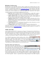
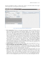
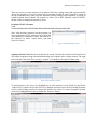
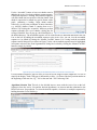
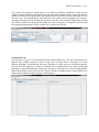
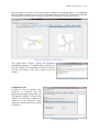
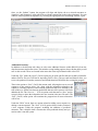
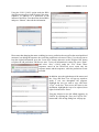
RNA Secondary
Structure Analysis
(RNASSA)
User Manual
By
RNAVLab, Bioinformatics Program
The University of Texas at El Paso
Updated: December 12, 2012
RNASSA 2.0 Manual: P. 2 of 11
RNASSA 2.0 Overview
RNASSA allows users to input RNA sequences either by loading a file in FASTA format or by direct
keyboard entries with options to select two prediction algorithms, RG and UNAFold. Prediction results
can then be visualized using PseudoViewer (pseudoviewer.inha.ac.kr) and compared to other RNA
structures. The RNASSA Graphical User Interface (GUI) is organized in tabs with different functions
with drop-down menus and toolbar icons. In this major upgrade, RNA Segmentation and Sequence
Assembly are the two powerful functions added in the first two tabs:
1. Input Tab is used for loading a FASTA file containing single or multiple RNA sequences.
For automatic RNA segmentation, only one file containing a single sequence is accepted.
2. Sequence Selection Tab is for creating a smaller Active List with a selected number of
sequences added from the Full List of sequences stored in the software. All the sequences in
the Active List are used for chunk editing or sequence assembly.
3. Algorithm Selection Tab is for submitting selected sequences from the Active List by
highlighting them, along with the desired algorithm(s), for RG and/or UNAFold predictions at
the RNAVLab (Ribonucleic Acid Virtual Laboratory). A table lists the sequences sent and the
current status of the process.
4. Visualization Tab allows for visualization of the prediction results with options to save the
image as a PNG file or to save the details in a text file.
5. Comparison Tab is used to compare two structures or sequences in the Active List.
Users may use RNASSA either by an anonymous login or an account with RNAVLab. For more
information, please visit www.rnavlab.utep.edu. In addition, RNASSA requires Java (version 6 or
later) running on Windows XP or later.
Menus and Tabs
Upon opening the RNASSA GUI, a login pop-up will appear. This login asks for the RNASSA user
name and password, these are the registered user name and password from the webpage. Upon entering
the correct information, press “Submit” and the program will bring you to the first tab. Pressing
“Cancel” will bring you into the program without logging in, the GUI will ask you to provide user
credentials at any point that a sequence is submitted or sequences are requested by the user.
To use RNASSA anonymously, click the checkbox before “Check to
login as guest” and then the “Submit” button, but data will be lost after
closing the program. Guest login analysis is for 1-time processing
whereas the account allows for retrieval of sequences and predictions
after logging off. Off-campus connections to UTEP still require a guest
VPN account from UTEP for RNASSA to access RNAVLab servers.
Figure 1: Login dialog box
Drop-Down Menus and Toolbar Icons:
Three menus (File, RNA, and Web Sequences) and
three icons (Load, Save, and Export) are located on
the top left-hand corner of the main GUI. The “File”
menu allows users to load or save RNASSA file with
Figure 2: Drop-down menus and icons
an “.rnassa” file extension, while the “RNA” menu
provides alternative ways to enter new, edit, or delete RNA sequence data with short-cuts Ctrl-N,
Ctrl-E, and Ctrl-D, respectively. The “Manual Cut/Edit (Ctrl-M)” is a manual segmentation utility
with powerful editing features to enter user-defined cut-points for creating or modifying chunks.
The “Web Sequences” menu is a powerful feature being developed to load RNA sequences
RNASSA 2.0 Manual: P. 3 of 11
directly from RNAVLab either by “Choose One” (Ctrl-C) or “Get All” (Ctrl-G). The “Login”
(Ctrl-L) option allows you to login in if you have not done so.
Input Tab: This tab is divided into four areas.
Figure 3: Input Tab for loading FASTA files and RNA Segmentation
1. RNA Segmentation: This box is developed from Segmenta (Version 2.0.121208) with four
buttons for automatic segmentation of one long RNA sequence. The first input field shows the
name of one single-sequence FASTA file loaded into RNASSA (see #4 below for loading a
FASTA file), while unsaved inputted sequences and loaded FASTA file with multiple sequences
are not accepted. A standalone Segmenta 2.0 is also available under “Manual Cut/Edit” of the RNA
menu or by pressing Ctrl-M. After entering necessary parameters, inversions can be found by
clicking “Find Inversions” button, and user can view the parameter file or the output file by hitting
“View Parameter File” or “View Output File,” respectively. Then, click "Run Segmentation" for
the GUI version of R to load, where you select "Source R Code..." under the File menu. Highlight
"Segmenta20.R" (with all methods) or "Segmenta21.R" (without using Optimized Method for
shorter running time), and click the file to run the program. Output text, FASTA, and PDF Rplot
files will be placed in subdirectory \inverslist. The FASTA files for chunks after segmentation can
be loaded directly back to RNASSA 2.0 for prediction.
2. Inputted Sequences: This shows the names and sequences either in the loaded FASTA file or of
the ones entered in the “Insert New Sequence” area below it.
3. Insert New Sequence (in FASTA format): This allows for the entry of one or more RNA
sequences. The correct format requires a “>” placed before the name of the sequence, followed by
the RNA sequence on the next line after a carriage return. Clicking the “Insert Sequence” button
will enter the typed text into the “Inputted Sequences” area above.
4. Full List: This shows the name of each sequence entered and/or loaded into RNASSA. The “Load
FASTA File” button will open a dialog box for loading files in the \RNASSA20 directory. If the
FASTA file contains a single sequence, the file name will also show up in the “RNA
Segmentation” file box. The “Sort and Remove Duplicates” button will sort the Full List by the
sequence names entered and remove any duplicated entries. The “Clear Highlighted Sequences”
button will clear the highlighted sequences in the Full List only without deleting them in the file.
RNASSA 2.0 Manual: P. 4 of 11
There are two ways to enter sequences to be analyzed. The first is typing a name and sequence into the
“Insert New Sequence” area (see Figure 4 below), and then pressing the “Insert Sequence” button on
the top right-hand corner of this area. This should be used for entering single sequences, or groups of
sequences pulled from GenBank. The second is to load a file of RNA sequences stored in FASTA
format, similar to loading a document by Word.
Example of FASTA Format:
>Test
ACUGUAGCUGAUGCUAGUCGUGCUGAUGAUGUAGCUGAUGUAGUCGAUCGA
Note: After inserting sequences into the program you
can sort the names of the sequences by pressing the
“Sort and Remove Duplicates” button. This sorts all of
the sequences by name, capital letters, and then
lower-case letters.
Figure 4: Insert New Sequence area
Sequence Selection Tab: This tab is divided into two areas. The left side of the tab is the Sorted List of
all available sequences along with information about each sequence in the varying columns. The right
side of the tab is the Active List, an active “playlist” of sequences with sequence names only.
Figure 5: Five sequences selected
To add sequences to the Active List, highlight one or more sequences in the Sorted List and hit the
“Add to Active” button on top of the Active List. Multiple selections can be done by holding down the
Ctrl key while clicking one item at a time or the Shift key for a block. To remove sequences from the
Active List, highlight them in the list and hit the “Remove” button.
Figure 6: Sequences added to the Active List
RNASSA 2.0 Manual: P. 5 of 11
For the “Assemble” button, at least two chunks must be
added to the Active List along with their parent sequence.
If the parent sequence is missing, the assembled sequence
will end with the last base position of the last chunk. Each
chunk is required to be named in a special format with a
prefix, containing a leading 3-digit chunk number
followed by its cut-point coordinates in interval notation,
e.g., 003[a,b] denotes Chunk #3 starting from a to b,
inclusive. By clicking the “Assemble” button to perform
sequence assembly for a set of chunks, a dialog box for
saving a RNASSA file will pop up with \RNASSA20 as Figure 7: Assembled sequence saved in RNASSA file
the default directory. The assembled sequence will be written in the file indicated and listed in the Sort
List on the left. By adding the assembled sequence to the Active List, you can view the assembled
sequence or its chunks by hitting the “Manual Cut/Edit” button. For viewing both the assembled
sequence and all the prefixes as shown in Figure 7 below, the assembled sequence must be highlighted
in sequence selector of the “Run Segmentation” dialog box invoked by clicking the “Manual Cut/Edit”
button or simply by Ctrl-M.
Figure 8: Pop up box showing the assembled sequence and its chunks in the Active List
For an assembled sequence, gaps are likely to exist but will be skipped if their lengths are over 100 to
simplify the display. Such a long gap is indicated by a tilde (~) in front of the base position number at
the beginning of the next line, e.g., ~901 at the start and ~3201 following 1500.
Algorithm Selection Tab: This tab is also divided into two areas with the Active List on the left.
Sequences from the Active List and the desired algorithm(s) are chosen and then submitted to the
RNAVLab server for prediction. To select the desired sequence, click on it (or multiple sequences by
holding down the Ctrl or Shift key).
Figure 9: RG and UNAFold selected for the three sequences
RNASSA 2.0 Manual: P. 6 of 11
Next, check the appropriate check boxes for the different prediction algorithms. Finally, hit the
“Submit” button to connect to the RNAVLab server and get the prediction results. Please note that any
submissions of the same sequence name and algorithm will be replaced by the last submission received
from the server. The right-hand side of this table gives the sequence name, algorithm used, start time,
and status of being processed with the time ticking. It may take a few seconds to display after clicking
the “Submit” button. Once the prediction is done, the status is changed to “Completed” with the finish
time and predicted structures will be available for viewing in the next tab.
Figure 10: Prediction jobs completed
Visualization Tab:
This tab allows for you to view the predicted fold using PseudoViewer. This tab is broken into two
identical parts. Within each part, a large viewing area is available below a drop-down list of the
different algorithms. Upon choosing the desired algorithm in which you have a predicted sequence,
you can select the sequence by name by looking at the second drop-down list. After selecting the
algorithm, an input field following “Starting at” will pop up, allowing you to use any starting number
instead of the default value. Next, press the “Submit” button to send the request for the PseudoViewer
image of the predicted secondary structure of the sequence.
Figure 11: Visualization Tab with a pair of PseudoViewer windows
RNASSA 2.0 Manual: P. 7 of 11
Once the image is received, it will automatically be displayed in the PseudoViewer. Two additional
buttons become available; the first is to save the original image to a PNG file. The image displayed has
been modified to fit within the viewing area, while the saved image is in the original size.
Figure 12: Predicted RNA structures displayed
The second button “Display” displays the information
regarding the sequence, i.e., sequence name, sequence, etc.,
in a new window. This information can also be saved in a
text file by clicking on the “Save” button in the new
window.
Figure 13: Data to be saved in a text file
Comparison Tab:
On this tab, you can compare either
sequences or structures and the
agreement percentage, along with a list
of comparison statistics. To start, select
whether you will either compare two
sequences or two structures. Then,
select the sequences that you would like
to compare.
Figure 14: Option panel of Alignments Tab
RNASSA 2.0 Manual: P. 8 of 11
Once you hit “Submit” button, the program will align and display the two selected structures as
Sequence 1 and Sequence 2 in the panel below with the comparison results in the right panel. You can
continue analyzing different sequences by selecting the appropriate ones and hitting “Submit” again.
Figure 15: Output for predicted structure alignment
Additional Functions:
In addition to the different tabs, there are also some additional features within RNASSA from the
drop-down menus and toolbar icons. This includes saving/loading options along with the ability to add
new or edit records. These are located in the menu bar at the top left-hand corner of the GUI.
Under the “File” menu, the “Open” (Ctrl-O) option is to be used with files that are created by RNASSA
and not FASTA files (see Tab One for importing FASTA files). The save and load features allow you
to save the predicted secondary structures and reload them into RNASSA after exiting the program.
There is the option to “Save” (Ctrl-S) the current work, allowing the user to save all
sequences in the current Active List, along with the information related to the
sequences, including sequence names and any predictions that were finished by the
time of the save. Please note that any predictions that are still in process will not be
added to the file. The “Save As…” (Ctrl-A) option works the same as “Save” option,
except it allows to place the information in a new location with a new file name. The
“Exit” (Ctrl-X) menu option will terminate the program but all unsaved material
will be lost.
Figure 16: File menu
Under the “RNA” menu, there are options related to adding a new sequence or
editing a current sequence. The “New” (Ctrl-N) option allows for the creation of
a new sequence within the program, including the addition of predicted
structures. This is helpful when a structure has been predicted already and you
need to enter it into the system.
Figure 17: RNA menu
menu
RNASSA 2.0 Manual: P. 9 of 11
Using the “Edit” (Ctrl-E) option under the RNA
drop-down menu allows modification of the name,
sequence, or addition of a prediction to the
instance of the RNA. First choose the desired RNA
and press “Submit,” then edit the information.
Figure 18: Choose RNA
Figure 19: Data entries for a new RNA sequence
Please note that changing the name or adding just a new prediction does not affect the stored predicted
structures, but editing the sequence does cause the predictions to be erased. Thus, if you do not want to
keep the original information, press the “Create New” button, otherwise use the “Replace Old” button
to replace the old predictions with the new ones. To save all information in .rnassa file, press “Done”
and select “Save” (Ctrl-S) under the “File” menu. Those
sequences stored on the RNAVLab server retain only the
sequence names and the sequences, while the predictions are not
recorded.
Figure 20: Replace, create, or discard
In addition, press the right-button of the mouse and
the “Copy and Paste” box will pop up anywhere
inside a text area throughout the program.
Highlight the text you want to copy and select
“Copy” in the box. Then, move the cursor to the
destination, highlight the text to be replaced, then
right-click and select “Paste.”
You may choose to save the edited sequence in
FASTA by clicking the “Save As FASTA File”
button and a file saving dialog box will pop up.
Figure 21: Editing the RNA sequence data
RNASSA 2.0 Manual: P. 10 of 11
Using “Manual Cut/Edit” (Ctrl-M) option under the RNA Menu, you can perform automatic or
manual segmentation. For automatic segmentation, click the “Run Standalone” button to launch
Segmenta 2.0 inside its frame. Automatic segmentation is also
available in the Input Tab as an integrated GUI within the “Run
Segmentation” area. The standalone version, however, is more
powerful in directory handling if the R installation on your
computer is not standard as the default is R2.14.2 for both 32and 64-bit.
For manual segmentation, you may add a single sequence to the
Active List and click “Manual Cut/Edit” to create chunks based
on user-defined cut-points. Each chunk will be named after the
given sequence name with the addition of a unique prefix
denoting its chunk number and cut-point coordinates as
described earlier in the Sequence Selection Tab, where the same dialog box can be invoked by a
similar button on the top of the Active List. During manual cutting, there are various suggested
default values for coordinates according to maximum chunk size provided by the user.
Figure 22: Create or edit chunks
If one or more chunks are present in the Active List, the sequence without prefix is assumed to be
the parent sequence. By highlighting the parent sequence in the “RNA Segmentation” dialog box
(see Figure 22 above), the prefixes of all the chunks present in the Active List will be shown in the
fields on top of the display pane for the parent sequence (see Figure 23 below). By default, long
gaps in assembled sequences will be shortened to simplify the display, but can be overridden by
selecting the radio button “Show Gaps in Full.”
Figure 23: Display of chunk prefixes and their parent sequence
By clicking a particular prefix, its original coordinates will show up in appropriate entry fields on
top for inputting cut-points and the prefix being edited is shown in red. During prefix editing, you
can always override the suggested default values.
RNASSA 2.0 Manual: P. 11 of 11
Using the four buttons at the top right-hand corner, you can add,
save, insert, or delete. For cases with over 20 prefixes, another
set of four buttons will become functional for forward and
backward navigation. By hitting the “Save” button, a dialog box
will appear with options to update only the Full and Active Lists
or to save also in a FASTA file (see Figure 24).
Figure 24: Update lists and save chunks
In addition, manual segmentation can also be used for cutting a very long sequence into regions by
clicking the radio button for “Region” on the top of the frame (see Figure 23). To distinguish regions
from chunks, the region number in the prefix begins with the letter R, e.g., R02 denotes region #2.
Future Features in Development:
The program is being further developed to benefit the user and make more of the RNAVLab
functionality available. Things that are in process are the ability to identify the type of pseudoknots,
and to extract sequences and structures from different databases. This is not an exhaustive list, and
suggestions to help make the program easier to use would be greatly appreciated.
Acknowledgements:
RNAVLab is supported by the Texas Advanced Research Program Grant 003661-0008-2006 and
003661-0013-2007; National Institutes of Health Grants S06GM08012-35, 5G12RR008124-11, and
3T 34GM008048-20S1; and National Science Foundation Grant DMS0800272. The original Java
codes of RNASSA GUI and user manual were developed and written by Jon Mohl, while prediction
algorithm modules on the RNAVLab server were implemented by Abel Licon and Leo Saldivar. We
also thank Reeder and Giegerich (2004) of pknotsRG (bibiserv.techfak.uni-bielefeld.de/pknotsrg) and
Markham and Zuker (2008) of UNAFold (mfold.rna.albany.edu/?q=DINAMelt/software) for their
source codes as well as Byun and Han (2009) of PseudoViewer (pseudoviewer.inha.ac.kr) for the
access. Please visit our RNAVLab (rnavlab.utep.edu) for more details and updated information.