Download TEX and/or

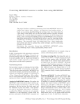
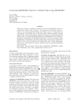
200
Péter Szabó
original
AutoTrace
Freehand
CorelTrace
Figure 2: AutoTrace compared to other tracing software
Streamline
original
-corner-threshold 80
-corner-threshold 90
Figure 3: AutoTrace cannot find corners at low resolution
AutoTrace with different parameters until the bug stops to manifest.
AutoTrace – although it is free – isn’t currently available from the web because of
technical reasons. So the proper version of AutoTrace is included in the TEXtrace
distribution.
AutoTrace was chosen for the tracing because it is free, works automatically, and
gives a good result (see Figure 2 for a comparison). Other examples of glyphs
traced by AutoTrace are the ornaments throughout this document. AutoTrace does
a quite good job at extremely high resolutions (such as the 7227 DPI used by TEXtrace), but produces poor and useless output for low resolutions (example: when
a glyph at 10pt is scanned at 600 DPI).
Figure 3 illustrates that the sharp corners produce the most problems for AutoTrace. Adjusting the command-line options doesn’t help, and it might even do
harm if different regions of the image require different options. Fortunately such
distortions do not occur when using TEXtrace, because fonts are rendered in a
high enough resolution.
6. The vector outlines are cleaned up a bit to comply the Type 1 specification.
The details of the cleanup have been explained in the previous item. The cleanup
after AutoTrace is much easier than it would be after METAPOST (see [3]).
The outlines are also properly scaled and shifted respect to the origin.
7. The outlines are merged into a Type 1 font file.
type1fix.pl (a utility bundled with TEXtrace) is run on the font file to fix
quirks in common font editors and other font handling software (including pdfTEX
and DVIPS).
The output .pfb file will be highly portable and compatible with most font
software. In an ideal world (with no Ugly Bits) there should be no font compatibility issues. However, in the real world, such issues are common since there is
no standard way to read a Type 1 font apart from interpreting it as a PostScript
program. (Of course that’d require a full PostScript interpreter in all font handling
programs, which is too complicated and would make execution slow).