Download GRAPES USER`S MANUAL

GRAPES USER'S MANUAL
GRAPES Tentative Ver 6.7
Original Japanese Manual developed by:
Katsuhisa Tomoda
This English edition is developed by:
Masami Isoda
Hiroki Yahara
Masaru Sanuki
Abednogo Sam Mbatha
January 2009
0
Users Manual
Operating Environment, Copyright, and Latest Version

Operating Environment
a. Operating Systems
WindowsNT/2000/XP/Vista
Operation under Windows95/98/Me has not been confirmed. Use of Ver 6.16 or earlier is
recommended under these operating systems.
b. Memory
256MB or more (512MB or more recommended).
c. Monitor
SVGA (800 x 600) or better
65,000 colors (16-bit color) or better
d. Hard Disk Drive
A floppy disk drive is sufficient if only GRAPES is required, however running from a floppy
disk drive is not recommended.

Copyright

GRAPES is freeware and may be copied, distributed and used without restriction.

Notification of distribution for commercial use is appreciated.

Copyright for GRAPES and the associated manual is held by Katsuhisa Tomoda.

Copyright for data and images created using GRAPES is held by the creator.


Cautions for Use
The author of this software assumes no responsibility for any results or consequence of its
use.

The author endeavours to eliminate bugs in the software, however this may not always be
possible.

Latest Version
The latest version of the software is available at the following URL:
http://www.osaka-kyoiku.ac.jp/~tomodak/grapes/
0H
1
Chapter 1 GRAPES Basics
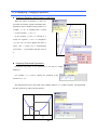
1-1 GRAPES Appearance

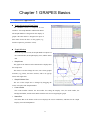
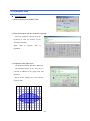
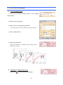
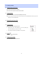
Graph Window and Data Panel
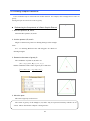
The GRAPES screen is composed of two
windows – the Graph Window and the Data Panel.
The Graph Window is designed for the display of
graphs. The Data Panel is designed for input of
data which forms the basis of the graphs (e.g.,
function equations, parameter values).

Graph Window
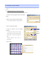
From the top of the screen, the Graph Window comprise of
the Control Pallet, the Graph Display Area, and the Status

Bar.
Control
Graph Area
Palette
The graph of the function in the Data Panel is displayed in
the Graph Area.
The mouse is used to change the Area, move basic graphic
Graph Area
elements (e.g. points), and move stickers, and to use pop-up
menus with right-click.

Graph Window Size
Status Bar
The size of the Graph Area is changed by dragging the
corner or border of the Graph Window.

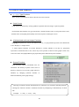
Control Pallet
The Control Pallet contains the Area Pallet for setting the Display Area, the Scale Pallet, the
Background Pallet, and the Tools Pallet with the tools for investigating the graph.

Status Bar
The Status Bar at the bottom of the screen displays the cursor coordinates, and hints for the Graph
Display Area and manipulation.
2


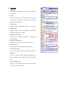
Menu Bar
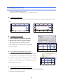
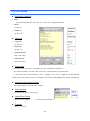
Data Panel
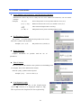
Menu Bar
Tool Bar
Four menus ([File], [Edit], [View], [Help]) are available in
the menu bar.

Toolbar
The toolbar contains seven function buttons focused on
file operations ([Initialize], [Open], [Save], [Undo],
[Redo], [Print], [Capture]).

FunctionArea
Handles function graphs displayed in the y = f (x) format.

Function Area
riaFunction
Relation Area
AaAAreaRelati
onRelationRelati
onRelation are
Parametric Curve Area
RelationArea
Handles graphs and areas expressed by equality and
Element Object Area
inequality equations of x and y.

Parametric CurveArea
Handles curves expressed by parameters, and graphs of
Parameter Area
polar equations.

Elementary Object Area
Handles points, circles, horizontal and vertical lines.

User Function Area
Parameter Area
Used for manipulation of parameters and images.

User Function Area
Used for entering an equation when defining a function.

NoteArea
Used for editting stickers displaying explanations on
the screen, scripts (a type of program), data tables, and text
notes.

Note Area
Line & Polygon Area
Displays setup information for linked graphic elements
(e.g., line segments, polygons).
3
Line & Polygon Area
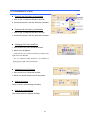
1-2 Saving and Loading Projects

Projects
Data created with GRAPES is referred to as a „project‟. A project includes data created with GRAPES
(e.g., graph equations, parameters, images, display areas, scale settings), and setup information.

Saving a New Project
Click on the
(Save) button on the Toolbar, or click
on [Save] in the [File] menu.

Save Under Another Name
Click on [Save As] in the [File] menu.

Load a Project (open file)
Click on the
(Open) button, or click on [Open] in the [File]
menu.

Open a Sample
Click on [Open Sample] in the [File] menu.
This menu is usable only if the GRAPES folder contains a
Samples folder.
What is a GRAPES project file?
A GRAPES project is saved with the „.gps‟ identifier. A GRAPES project file includes all the data
necessary to run GRAPES. GRAPES image data has the same file name as the project file, however it is
saved with the „.gpp‟ identifier. Loss of the the image file will not present a problem if the project file is
available.
Compatibility of project files is maintained when upgrading GRAPES to a new version, and existing
data can therefore be used without problems.
4
1-3 Initializing a Project and Changing Default Values, and Associating
Files

Initializing of Project
Click on the
(Initialize) button, or click on [Initialize] in
the [File] menu.
All data currently in preparation is deleted, and the system returns to
the condition at startup.
Data already saved is not deleted.

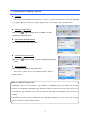
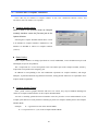
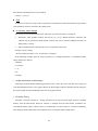
Changing Default Values
All values are initialized to the default values at startup and at initialization.
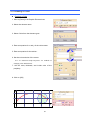
1. Select values to be set as defaults.
Default data which may be changed includes most
optional settings (e.g., settings related to display areas,
window size, and scales).
2. Click on [Set Default] in [Environment] in the
[Edit] menu.

Initializing Default Values
Click on [Initialize Default ] in [Environment] in the [Edit] menu.
The defaults selected by the user are returned to their original values.

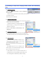
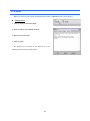
Associating Files
If files have been associated, GRAPES may be
started, and the file opened, simply by double-clicking
on the GRAPES project file („*.gps‟).
Click on [File Association] in [Environment ] in the
[Edit] menu.
The GRAPES project file icon is changed to the
„bunch of grapes‟ icon. Note that this change in the icon
may occur only after restart in some cases.
☆ Under Windows Vista, the operation described above is
accomplished by first closing GRAPES, right-clicking on the
icon, selecting [Run as Administrator], and then restarting.
5
Chapter 2 Function Graphs
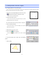
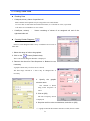
2-1 Creating and Adding Function Graphs

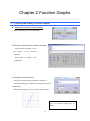
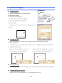
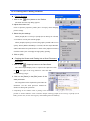
Adding and Creating Function Graphs
1. Click on [Draw] in the Function Area.
2. Enter the equation with the scientific calculator.
Enter from the keyboard or with
the
buttons
on the
scientific
calculator.
When input is complete, click
on[DefEnd].
3. Properties of the graph style.
The Function Graph Property Window is displayed.
See the following page for details of setting the graph color
and thickness.
When all the settings have been entered, click on [OK].
Up to 20 function graphs may be
drawn.
6
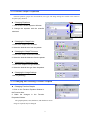
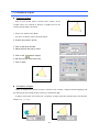
2-2 Function Graph Properties
Function equations, graph color and thickness, line type, and image settings are entered in the Function
Graph Property Window.

Changing Equations
1. Click on the Function Equation Window.
2. Change the equation with the scientific
calculator.

Changing the Graph Color
1. Point to the Graph Color Window.
2. Select the desired color from the palette.

Changing the Graph Thickness
1. Point to the Graph Thickness Window.
2. Select the desired thickness from the palette.

Changing the Graph Line Type
1. Point to the Graph Line Type Window.
2. Select the desired line type from the palette.

Changing the Image Settings
Click on [AfterImg].
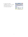
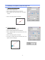
2-3 Changing and Deleting Function Graphs

Changing Function Graphs
1. Click on the Function Equation Window in
the Function Area.
2. Make the changes in the Function
Properties Window.
The graph equation, color, thickness, and whether or not an
image is required, may be changed.
7

Deleting Function Graphs
1. Right-click on the Function Equation
Window in the Function Area.
2. Select [Delete] from the pop-up menu.
3. Click on [OK] to confirm delete.
8
2-4 Moving the Graph

14 Parameters
The following 14 letters may be assigned to parameters.
a , b , c , d , k , m , n , p , q , s , t , u , v , 
A parameter is displayed if it is appropriate to change its value.

Increasing and Decreasing Parameter Values
Click on the
(increase and decrease) buttons.
☆ The value changes continuously when a button is held down.

Range of Increase/Decrease
Click on the
(range of increase/decrease) buttons.
☆Click on the Range of Increase/Decrease Window to enter the
value from the keyboard.

Changing the Rate of Increase/Decrease
Move the slider to change the rate of increase/decrease.
Changes the rate at which the value is changed when the
increase/decrease buttons is held down.

Substituting Values in Parameters
Click on the Parameter Window to enter the value from the
keyboard.
☆ Double-click to use the Scientific Calculator.

Changing the Method of Increase/Decrease
Click on [+].
Parameter changes 1->2->3->4
Parameter
changes 1->2->4->8

Synchronizing Parameters
It is possible to synchronize parameters so that changing one
parameter changes other parameters.
9
1. Click on the
(synchronize) button for all the parameters
to be synchronized.
2. Increasing and Decreasing Parameter Values
Values of other linked parameters are increased/decreased.
In the example at right, increasing/decreasing value a
increases/decreases value b.
10
2-5 Leaving a Graph – the Afterimage
The graph can be changed by increasing/decreasing the parameter values. The Afterimage is used to leave a
record of the original graph.

Leaving an afterimage
1. Click on the graph of the function equation for which the afterimage is required.
2. Click on [Afterimg].
3. Click on [OK].
4. Change the parameter.

Temporarily Halt Afterimage Recording
Click on the
button (Parameter
Area
Afterimage OFF).
The button will remain pressed, and the Afterimage
will not be recorded. Click again to clear.

Create Afterimage
Click on the
button (Create Afterimage of
Parameter Area).
It is possible to record Afterimages of all currently drawn graphs.
11

Deleting the Afterimage
Click on the
button (Delete Afterimage of
Parameter Area).
12
Chapter 3 Display Area and Scale
Adjustment
3-1 Enlarging the Graph

Changes to the Area - Enlarging the Graph
1. Click on the
button (Zoom in).
The Zoom in button is selected.
This status is referred to as as the Enlarge Mode.
Click again to clear the Enlarge Mode.
2. Specify a rectangular area.
At one end of a diagonal in the rectangular area, and
a. left-click,
b. drag while holding the left button down,
c. and then, release at the other end of the diagonal.

The aspect ratio is fixed when enlarging. Change the aspect ratio with Shift key + drag.

Use the Ctrl key + drag to enlarge with the point at which the mouse is clicked at the center.

Double-click on the center of the area to be enlarged to double the size of the graph.
13
3-2 Shrinking the Graph

Changes to the Area – Shrinking the Graph
1. Click on the
button (Zoom out).
The Zoom out button is selected.
This status is referred to as as the Shrink Mode.
Click again to clear the Shrink Mode.
2. Specify a rectangular area.
The graph is shrunk into the specified rectangular area.
At one end of a diagonal in the rectangular area, and
a.
left-click,
b.
drag while holding the left button down,
c.
and then, release at the other end of the diagonal.
The reduced image of the graph is displayed on the screen.
Use it for reference.

The aspect ratio is fixed when shrinking. Change the aspect ratio with Shift key + drag.

Use the Ctrl key + drag to enlarge and shrink with the point at which the mouse is clicked at the center.

Double-click on the center of the area to be shrunk to halve the size of the graph.
14
3-3 Moving the Graph
Changes to the Area – Moving the Graph

1. Click on the
button (Move).
The Move button is selected.
This status is referred to as as the Move Mode.
Click again to clear the Move Mode.
2. Specify a rectangular area.
Anywhere in the Graph Window,
a.
left-click,
b.
drag while holding the left button down,
c.
and then release at the other end of the diagonal.
A copy of the graph moves.
Determine the amount of movement required.

If using a mouse with a scroll wheel, push the wheel and drag to move the graph. This
eliminates the need to select the Move Mode.
15
3-4 Changes to the Area – 1:1, Undo, Redo

Fix the aspect ratio to 1:1
Click on the
button (1:1).
Changes the aspect ratio of the graph to 1-to-1.

Undo a Change to the Area
Click on the
button (Undo of Domain).
Returns to the immediate previous display.
Up to 50 consecutive Undo operations are possible.

Redo a Change to the Area
Click on the
button (Redo of Domain).
Cancels an Undo operation.
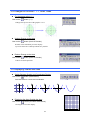
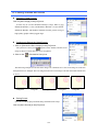
3-5 Displaying Scales and Axes

Switch Between Scales and Coordinates Display
Click on the
button (Graduations).
Switches between a scale and coordinates.
y
y
1
1
-1
O
-1
1 x
-1
O
y
1 x
O
y
x
O
x
-1
y

Displaying the Axes Outside the Area
Click on the
button (Out Area Graduations).
Click again to clear the display.
x
16
3-6 Changing Scale Ranges

Changing Scale Ranges
Click on the
button (Shrink x Axis Scale Range) to shrink the range of the scale on the x
axis.
Click on the
button (Expand x Axis Scale Range) to expand the range of the scale on the x
axis.
Click on the
button (Shrink y Axis Scale Range) to shrink the range of the scale on the y
axis.
Click on the
button (Expand y Axis Scale Range) to expand the range of the scale on the y
axis.
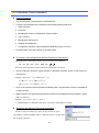
The scale range changes as follows:
1 → ×2 → ×5 → ×10
1 → ×1 → ×1 → × 1
5
2
10
Note that the scale range changes as follows when the base values are π, 2 , 90 and 180 etc.
1 → ×2 → ×3 → ×6 → ×9 → ×18 → ×45 → ×90
1 → ×1 → ×1 → ×1 → ×1 → × 1 → × 1 → × 1
3
6
2
9
18
45
90

Changing the Spacing of the Scale Notation
Click on

or
while holding down the Ctrl key.
Changing the Size of Scale and Label Notation
Click on the
button (Change Scale Notation Size) on the
Scale Pallet.
17
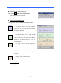
3-7 Standard Settings for Scales and Areas

Displaying the Options Window
Click on the
button (Area Pallet Options).
The Options Window is displayed.

Using the Standard Settings
Click on one of the four settings displayed to select it.
Set angles in radians, and 1 as the standard
value for x and y axis scales. This is the default
settings for GRAPES.

Set angles in radians, and 2 as the standard
value for the x axis scale. Select when drawing
graphs of trigonometric functions with the
circular method.
Set angles entered with the frequency
method, and 90 set as the standard value for the
x axis scale. „º‟ added to the angle on the x axis
scale.
Select
when
drawing graphs
of
trigonometric functions with the frequency
method.
Displays a polar coordinate scale.

Completing Setup
Click on [OK].
18
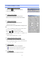
3-8 Detailed Settings for Scales

Displaying the Scale Setup Window
1. Click on the
button (Area Pallet Options).
2. Click on the [Scale] tab.

Setting Up Scale Displays
Clear the check from [Lines] to remove grid lines.
Clear the check from [Letters] to remove scale notation.

Setting Up Axis Displays
Clear the check from [Axis] to remove the axis.
The letters is also removed.
Overwrite the letters in the Label Window to change the axis
label.
„x‟ and „y‟ are displayed by default as the axis labels, however
these may be overwritten with any desired labels.
Click on
x or  to change the x axis variable.
If  is selected as the axis variable,  is handled as an
independent variable.
Used for displaying graphs such as y  sin  .

Setting Up Standard Values for Scales
Enter the standard value in the Standard Value Window.
The scale width normally changes as follows based on this value.
1 → ×2 → ×5 → ×10

Setting Up Letters
Select the position for the letters to be displayed.
If
is selected, the letters is displayed between grid lines.
If
is selected, the letters is displayed over grid lines.

Fractional Letters
If
is selected, the letters is displayed as fractions.
19
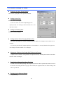
3-9 Detailed Settings for Areas

Displaying the Area Setup Window
Click on the [Area] tab in the Options Window.

Setting Screen Size
Enter the width and height.
Screen size is the size of the Graph Display Area.
Specify screen size in integer values between 150 x 150
and 1600 x 1600.

Setting the Drawing Area
Enter the x and y ranges.

Setting Options When Changing Window Size
By default, the graph size remains unchanged and the display area changes, when window size is
changed.
If a check is placed in the [Adjust Graph Size when Window is resized] checkbox, the graph size
also changes when the window size is changed.

Aligning the Position of the Scale With Pixels on the Screen
Adjusts the area so that the scale grid lines are aligned accurately with the pixels on the screen when
the scale value is an integer.

Read Out the Window Size When File Open
As to the screen size when opening a file, only the aspect ratio will be reproduced, not the screen size
at the time of creating the file. If you give this a check, the original screen size when creating a file
will be reproduced.

Returning to the Status at Startup
Click on [Initialize].
20
Returns to the screen size and drawing area size at startup.

Completing Setup
Click on [OK].
21
Chapter 4 Relation Graphs
4-1 Creating and Adding RelationGraphs

Creating and Adding Relation Graphs
1. Click on [Draw] in the Relation Area.
2. Enter the equation with the Scientific Calculator.
Enter the equality equation from the
keyboard or with the buttons on the
scientific calculator.
When input is complete, click on [DefEnd].
3. Set the graph style
The Relation Property Window is displayed.
See „2-2 Function Graph Properties‟ for methods of
changing the graph color and thickness.
When all the settings have been entered, click on [OK].
y
O
x
Up to nine relations may be drawn.
22
4-2 Inequality Area

Inequality Area
1. Click on [Draw] in the Relation Area.
2. Enter the equation with the Scientific Calculator.
Enter the inequality equation from the
keyboard or with the buttons on the
Scientific Calculator.
When input is
complete,
click on
[DefEnd].
3. Properties of the graph style
The Relation Property Window is displayed.
The hatching pattern for the area may be
selected in addition to the graph color and
thickness.
When all the settings have been entered,
click on [OK].
y
O
x
23
4-3 Union of Overlaps of Multiple Areas

Displaying Overlap of Multiple Areas
y
Joins the inequality equation for each area with AND.
Example：( x 2  y 2  2 2 ) AND (  1  x  y  1 )
The above may be expressed as C1 : x 2  y 2  2 2 , C2 :  1  x  y  1
O
x
C3 : C1 AND C2

y
Displaying Unions of Multiple Areas
Joins the inequality equation for each area with OR.
Example：( x 2  y 2  2 2 ) OR (  1  x  y  1 )
O
The above may be expressed as C1 : x  y  2 , C2 :  1  x  y  1
2
2
2
C3 : C1 OR C2
☆ AND takes priority when AND and OR are mixed.
☆ Parentheses cannot be used for nesting of union and common sets.
The following expressions are therefore not permitted.
Example 1：(C1 OR C2) AND C3
Example 2：C1 OR (C2 AND C3)
Note that the area in Example 2 can be drawn as [C1 OR C2 AND C3].

Handling of Boundary Lines
As with x 2  y 2  2 2 , when the boundary line expressing the
inequality equation is not included in the area, the boundary line is
displayed in a pale colour. Manipulation of function properties allows
display of the pale boundary lines to be suppressed.
y
y
O
O
x
24
x
x
4-4 How to Draw Relations

y  f (x ) Type Functions
These are the actual Relations, and are therefore the easiest to draw.

Conic Curves
Conic curves are obtained by solving quadratic equations and converting to explicit equations.
For functions other than the two types noted above, find the function value at each point on the screen,
and draw after investigating the boundary line between positive and negative areas.

10-dimensional and Less Integer Functions
Lagrange interpolation is used for calculation when x or y is a polynomial expression of ten dimensions
or less. Display is a simple matter.
☆ With complex functions it becomes difficult to evaluate whether or not they are polynomial
expressions of ten dimensions or less, and it may not be possible to draw accurate graphs. In this case,
remove the check from [Rapid Drawing in polynomial] in the Relation Properties Window.

General Functions
Some functions require considerable time for
calculation. The density of points on the screen is
therefore reduced. If an accurate graph cannot be
obtained, try changing [relations: Number of
Int.Points Relation] in the graph settings.
Drawing of relations assumes that functions are continuous. For functions including fractions,
rearrange the fraction to obtain a continuous function by multiplying a denominator(s) for both
side.
Example： x  tan y  x cos y  sin y
25
Chapter 5 Points and Locus
5-1 Drawing a Point

Drawing a Point
1. Point the cursor
to [Draw] in the Graphic Element Area.
2. Select the element name.
3. Select a point from the element types.
4. Enter an equation for x.
5. Enter an equation for y.
6. Set the graph style.
See the following page for details of
changing point color and size.
7. When all the settings have been entered, click on [OK].
Locus cannot be drawn yet. To draw a locus, the afterimage and the thickness of the locus
must first be set, and parameters changed.

Simple Drawing of Points
Points can be drawn more simply if coordinates are provided as numerical values rather than as
equations,
See „5-7 Points and Dragging‟.
26
5-2 Properties of Points

Entering and Correcting x Coordinates
1. Click on the x Coordinate Equation Window.
2. Correct the equation with the Scientific Calculator.

Entering and Correcting y Coordinates
1. Click on the y Coordinate Equation Window.
2. Correct the equation with the Scientific Calculator.

Changing Point Color and Size
1. Point to the Point Color and Size Window.
2. Select from the palette.
Points may be set as white-on-black by pointing to the
right of the Size Window.
See „2-2 Function Graph Properties‟ for methods of
changing the graph color and thickness.

Changing Locus Thickness
1. Point to the Locus Thickness Window.
2. Select the desired thickness from the palette.

Setting the Image
Place a check in the [AfterImg] checkbox.

Setting the Label Display
Click at the position to display the label.
27
5-3 Locus and Afterimages

Locus and Afterimages
1. Click on the equation display section of the Graphic
Element Area.
2. Select the locus thickness.
3. Place a check in the [AfterImg] checkbox.
The image may be left even without an image of the point.
4. Click on [OK] to finish.
5. Change the parameter.
When the parameter is changed the point image remains
and the locus is drawn.





Deleting the Image and the Locus
Click on the
button (Clear All Afterimage).
28
5-4 Making Use of Locus
Locuses are broken lines joining points.
Existing locii may only be hidden, deleted, or changed in density.

Drawing Smooth Locus
Locuses simply join points, and are therefore drawn smoothly by reducing the difference between
points.
y
y




P
1
O

Difference between points =
Difference between points =


P
0.2


O
x
x
Changing Locus Density
1. Click on [Options] on the Afterimage Pallet.
2. Select image density in the graph settings.
This change is applied to all images and locii.
y
Color and thickness of existing locuses and images

cannot be changed.

P

O


Hiding Specific Afterimages and Locuses
Click on the element name in the Graphic Element Area.
Element names are assigned buttons in the Graphic Element
Area. These are referred to as „display switches‟. Use display
switches to permit instantaneous switching between display
and non-display of elements.

y


O
Deleting Specific Afterimages and Locuses
1. Right-click on the function equation display section of the Data Panel.
2. Select the afterimage to delete.
29


x
x
5-5 Drawing a Circle

Drawing a Circle
1. Point to [Draw] in the Graphic Element Area.
2. Select the element name.
3. Select Circle from the element types.
4. Enter an equation for x and y of the circle center.
5. Enter an equation for the radius r.
6. Set the color and size of the center.
See „2-2 Function Graph Properties‟ for methods of
changing color and thickness.
7. Set the color, thickness, and inside color of the
periphery.
8. Click on [OK].
y


O
P

 x
30
5-6 Drawing Horizontal and Vertical Lines

Drawing Horizontal Lines
1. Point to [Draw] in the Graphic Element Area.
2. Select the element name.
3. Select a horizontal line from the element types.
4. Enter the y coordinate of the horizontal line.
5. Enter the width if required.
6. Set the color and size of the line.
See „2-2 Function Graph Properties‟ for
methods of changing color and thickness.
7. Set the inside color if the line has a width.
8. Click on [OK].

Drawing Vertical Lines
Same as for horizontal lines.
31
5-7 Points and Dragging

1 Right-click
Drawing a Point
1. Right-click at the position to draw the point.
2. Point to [Set Point].
2 Point
3. Select the point and click.
3 Click
The Point Property Window is displayed.
4. Set the color and size of the point.
5. Click on [OK].
Point R has been selected here, however the same applies to
all points.

Dragging a Point
When a numerical value is the basis of a basic graphic element it may be moved by dragging.
1. Point to the point.
The shape of the cursor changes when the point is able to be dragged (see diagram at bottom-left).
2. Drag with the left button.
a. The point may be dragged when a check
b. The point cannot be dragged when a check has
has been placed in the the [Draggable].

not been placed in the [Draggable] checkbox.
Dragging a Circle
The circle moves when its center is dragged. The circle radius changes when its periphery is dragged.

Dragging a Point on a Curve
A point on a curve may be dragged. See „6-1 Parameter Display Curves‟.
32
Chapter 6 Curves
6-1 Parameter Display Curves

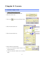
Drawing a Parameter Display Curve
1. Point to [Draw] in the Parametric Curve Area.
2. Select the element name.
3. Click on the
button (Curve) in Element Types.
4. Enter a function equation for x.
5. Enter a function equation for y.
6. Set the notation for the parameter.
a. Point to the Parameter Notation Window in the
Variable Range Area.
b. Select the parameter notation from the Notation
Pallet.
33
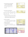
7. Set the variable range for the parameter.
Click on the Variable Range Window
and enter the variable in the Scientific
Calculator. The top and bottom limits of
the
variable
range
may
be
set
individually.
8. Set the range of increase/decrease.
The curve becomes smoother as the range of
increase/decrease is reduced. Note that GRAPES requires that
(variable range top limit – bottom limit) / range of
increase/decrease ≦ 5000.
★［ If you check “Synchronize”, the value of parameter
of Data Panel will be restricted with the range set here.
Also note that the increment value set here is
synchronized with that of parameter of Data Panel.
9. Set the curve properties.
Set color, thickness, line type, inside color, and image.
See „2-2 Function Graph Properties‟ for methods of
changing color and thickness.
10. Set the point properties.
Points moving on a curve may be drawn.
★ Points on the curve may be dragged when [Draggable]
is checked.
y
P
O
x
34
11. Set the label.
Set the label notation and the display position.
12. Click on [OK].
35
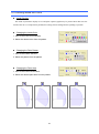
6-2 Painting Inside the Curve

Inside Painting
The inside of parameter display curves and polar equation graphs may be painted. Note that since the
inside of the curve is transparent by default, this setting must be changed before painting is possible.

Changing the Inside Color
1. Point to the Inside Color Window.
2. Select the desired color from the palette.

Changing the Paint Pattern
1. Point to the Pattern Window.
2. Select the pattern from the palette.

Changing the Paint Area
1. Point to the Paint Area Window.
2. Select the desired paint area from the palette.
36
6-3 Polar Equation Graphs

Drawing a Polar Equation Graph
1. Point to [Draw] in the Curve Area.
2. Select the element name.
3. Click on the
button (Polar Equation) in Element Types.
4. Enter an equation for r using θ.
5. Set the variable range and range of increase/decrease for θ.
Click on the Variable Range Window and
enter the variable in the Scientific Calculator.
The top and bottom limits of the variable range
may be set individually.
6. Set the curve, point, and label properties.
7. Click on [OK].
P
O
x
37
6-4 Negative Radius Vectors

What is a Negative Radius Vector?
With polar coordinates, the location of a point is expressed in terms of the radius vector – the distance
from a pole (the origin), and the angular displacement – the angle from the start line (the x axis). The radius
vector can therefore only be a value of 0 or greater. On the other hand, it is sometimes convenient to allow
negative radius vectors for polar equations. In such cases, points are taken in the direction opposite to the
conventional direction (see diagram at bottom-right), and the radius vector is negative at initialization.
(r ,  )  ( r ,   ) when a negative radius vector is allowed.
where, r  0
where, r  0
r





x
|r|

x
Disallow Negative Radius Vectors
Remove the check from [Allow negative radius] under
the [Function] tab in the Options Window.
The following graphs for r  sin 2 illustrate
the cases of a negative radius vector allowed (left),
and not allowed (right).
In subsequent graphs, the part for which the radius vector is negative will not be drawn.
O
x
O
38
x
6-5 Relations and Polar Equations
Since the radius vector r and angular displacement θ may be used with relations, they may also be used in
drawing graphs of polar equations.

Relations and Polar Equations
1. Place a check in the [Handle theta as argument in
Relation] checkbox under the [Function] tab in the
Options Window.
θ is then angular displacement rather than a parameter.
2. Click on [Draw] in the Relation Area.
3. Enter the equation with the Scientific Calculator.
Enter the equation using the radius vector r, and the angular displacement θ.
( a certain portion is hidden in the above sentence)
4. Subsequent operation is the same as for Relation graphs.
y
O

x
Handling the Radius Vector and Angular Displacement in Relations
The range of angular displacement  is 0    2 or       . In either case, it is set in [Range
of Angle] under the [Function] tab in the Options Window.
Negative radius vectors are not allowed in relations.
39
Chapter 7 Linked Graphic Elements
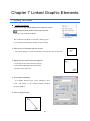
7-1 Linking Two Points

Linking Two Points
1. Right-click in the Graph Display Area and click on the
(Connect Points) button on the pop-up menu.
This selects the Link Points Mode.
The Connect Points Mode is cleared by clicking again,
or by clicking on the Enlarge, Shrink, or Move buttons.
2. Point to one of the points with the mouse.
The cursor changes to a pen icon when the cursor is moved over the point.
3. Specify the two ends of the line segment.
a. Left-click on one end of the line segment.
b. Drag while holding the left button down.
c. Release at the other end.
4. Line Segment Settings
Set Graphic Element type, Color, Thickness, Area
Color, and Image in the Linked Graphic Element
Property Window.
5. Click on [OK] to finish.
40
7-2 Changing and Deleting Linked Graphic Element Properties

Changing and Deleting Linked Graphic Elements
1. Click on the relevant graphic element in the Linked
Graphic Element Area.
Or, right-click on the linked graphic element and then
click on [Linked Graphic Element Properties] on the
pop-up menu.
2. Set the type, color, thickness, area color, and image of the graphic element.
Click on [Delete] to delete.
3. Click on [OK].

Graphic Element Types
Line segment
Straight line
Half-line
Arrow
Parenthesis
Deletion of a single point in a graphic element will delete the element.
41
Rectangle
7-3 Drawing Broken Lines and Polygons

Displaying Broken Lines and Polygons
Three or more points must be drawn before starting. In the example below the method of drawing a triangle
based on the three existing points P, Q, and R is described.
1. Right-click in the Graph Display Area and click on the
(Connect Points) button on the pop-up menu.
This selects the Link Points Mode.
2. Link the two points P and Q.
Click on the left button on the point P, drag to Q while
holding the button down, and release.
The Linked Graphic Element Property Window is displayed.
3. Click on the Apex Window.
The pop-up window is opened to display a list of apexes
which may be specified.
4. Select [R] from the pop-up menu.
5. Click on the
Click on the
button (Polygon).
button (Broken Line) to draw a broken
line.
6. Set the boundary color, inside color, and hatching
pattern.
7. Click on [OK].
42
7-4 Displaying Angles

Displaying Angles
Three or more points must be drawn before starting. In the
example below, the method of drawing ∠ PQR based on the
existing triangle PQR is described.
1. Select the Link Points Mode.
See above for details of the Link Points Mode.
2. Link the two points P and Q.
3. Click on the Apex Window.
4. Select [R] from the pop-up menu.
5. Click on the
button (Angle).
6. Set the line color and inside color.
7. Click on [OK].

Orientation of Angles
Angles are displayed in counter-clockwise orientation. For example, ∠PQR is formed beginning with
the half-line QP, proceeding counter-clockwise to the half-line QR.
To display only angles of less than 180º, set [Range of Angle] under the [Function] tab in the Options
Window to [     ].
43
7-5 Displaying Line Segment Length and Angle Size

Displaying Line Segment Length
1. Click on the line segment PQ.
2. Click on [Linked Graphic Element Properties].
3. Select “!{[PQ]}” from the pull-down menu in the Label
Window.
4. Click on the display position of the label.

Displaying Angle Size
1. Right-click on the arc of the angle.
2. Click on [Linked Graphic Element Properties].
3. Select “!{[arg(P,Q,R)]|3}” from the pull-down menu in the
Label Window.
4. Click on the display position of the label.
5. Set [Unit of Angle] under the [Function] tab in the
Options Window to [Degree].
44
Chapter 8 Mutual Referencing of
Function Graphs
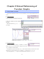
8-1 Using Defined Functions
A function may be defined as f(x) when it is to be used repeatedly. Up to five of these defined functions may
be used.

Defined Functions
1. Click on [Draw] in the Defined Function Area.
2. Enter the equation with the Scientific
Calculator.
Eight defined functions (f, g, h, f1, ….. , f5)
are available.
A graph of the two functions y  f (x ) and y  f ( x  p )  q

Bivariate Functions
A function including the variable y is handled as a bivariate
function. In this case, the function label is displayed in the format
“f(x,y)” to indicate a bivariate function.
Two arguments are passed in the format “f(2x,y) ” when a bivariate function is referenced. The second
argument may be omitted, and in this case it is handled as y=0, and therefore f (x) = f (x , 0).
Up to four arguments (x, y, z, w) may be used, and the function is therefore f ( x, y , z, w) .
45
8-2 Referencing Functions

Referencing Functions
y
The diagram at left shows the graphs of two
functions y1 = sin ax and y2 = cos bx,
and the synthesized function
O
x
y3 = sin ax + cos bx.
In this case, processing speed is increased if the
format: y3 = y1 + y2 is used.
Furthermore, when investigating synthesis of
another function, simply substituting for y1 and y2 facilitates reuse of
data.

Reference Sequence
Care must be taken with the sequence in which the function
y
is referenced.
For example, the same graph may be drawn with
O
y1  y 2  y3
x
and y 2  sin ax ， y 3  cos bx

Circular Referencing
The type of referencing able to be used is restricted. Care
is required with circular referencing of functions. An error
message is displayed when circular referencing is found,
and input is cancelled.
Functions may be referenced from relations, however processing speed is reduced. Functions
cannot be referenced from basic graphic elements and curves.
46
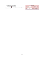
8-3 Dragging Graphs – Coordinate Referencing
Point coordinates may be referenced from a function.
For example, a quadratic equation moved by dragging the apex A may be drawn.

Dragging a Graph
1. Draw point A
See „5-7 Points and Dragging‟ for details of drawing points.
2. Use the point coordinates to draw the graph of the quadratic equation.
The coordinates of the point A are (A.x, A.y).
The quadratic equation with the apex at point A
is therefore:
y  a ( x  A.x ) 2  A.y .
3. Drag point A.
The graph moves when the mouse button is released.
47
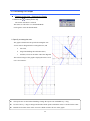
8-4 Linking Graphic Elements
Point coordinates may be referenced from another function. For example, draw a triangle and its center of
gravity.
Moving the apex also moves the center of gravity.

Referencing the Components of a Basic Graphic Element
1. Draw the apexes A, B, and C.
Draw the three points A, B, and C.
2. Link the apexes A, B, and C.
Edges are unnecessary, however drawing them gives the triangle
form.
See „7-3 Drawing Broken Lines and Polygons‟ for details of
drawing triangles.
3. Determine the center of gravity G.
The coordinates of points A, B, and C are
( A.x , A.y ), ( B.x , B.y ), ( C.x , C.y )
and the coordinates of the center of gravity G are therefore
 A.x  B.x  C.x A.y  B.y  C.y 
,


3
3


4. Move the apex.
The center of gravity G also moves.
The center of gravity of the triangle A, B, and C may be expressed concisely with the use of
vectors. This is described in „Chapter 9 Using Vectors‟.
48
Chapter 9 Using Vectors
9-1 Points and Vectors

Points and Vectors
The center of gravity G of the triangle ABC is expressed in coordinates as follows.
 A.x  B.x  C.x A.y  B.y  C.y 
,


3
3


This is expressed in position vectors as follows.
OA  OB  OC
3
This is also possible in GRAPES.
OA  OB  OC or A  B  C
3
3
Points and vectors are considered to be the same in GRAPES.

Vectors and Real Numbers
A vector is created from two real numbers enclosed in
parenthesis. For example, the vector having an x component of
2 and a y component of 3 is expressed as follows.
( 2, 3 )
This is the same as coordinate notation.
On the other hand, when a vector is provided, „.x‟ and „.y‟
are added to the components.
( 2, 3 ).x = 2
( 2, 3 ).y = 3

Points and Displacement Vectors
A displacement vector is expressed by drawing a basic graphic element and
points on a curve together. For example, the two points P and Q are expressed as
PQ .
49
9-2 Entering in Vector Notation
The use of vectors allows the position of a point to be entered without the need for separate x and y
coordinates.

Entering the Position of a Point Using Vectors
First, draw the triangle ABC before beginning the following operation.
1. Create the new basic graphic element G, and select
[Point].
2. Place a check in the [Use Vectors] checkbox.
The two Equation Windows are merged into one.
3. Click on the Equation Window.
4. Enter the equation with the Scientific
Calculator.
The Scientific Calculator is able to handle
vector equations. The center of gravity of the
triangle ABC is entered in the example at
right.
Entering
equations
using
vectors
is
described later.
5. Click on [OK].
y
A
G
B
C
O
x
50
9-3 Vector Calculations

Vector Addition and Subtraction, and Real Number Multiples
Mathematical notation may also be readily used for vector addition and subtraction, and real number
multiples.
Examples

P+(-4,5):
Sum of the position vector of point P and the vector (-4,5).
( 2,3)  ( 4,5) :
Difference between the vector (2,3) and the vector (-4,5).
3 PQ :
Three times the displacement vector PQ.
( A  B) / 2 :
Mid-point between points A and B (position vector).
Dot Products of Vectors
The operator ・is used in finding the dot product of two vectors.
Enter the * symbol on the keyboard.
Example (1,2)・(3,4):

Dot product of (1,2) and (3,4).
Mixed Operation
Complex calculations are possible with the use of
parentheses.

Size of Vectors
The same symbol as the absolute-value symbol is used in finding vector
size (length). This is also mathematical notation.
Enter the [ and ] symbols on the keyboard.
Example |(3,4)|:

Size of vector (3,4).
Line Segment Length
‘[PQ]’ represents the size of the displacement
vector PQ , however it is displayed simply as ‘PQ’.
This represents the length of the line segment PQ.
51
9-4 Distances and Angles

The len Function Returns Distance
len ( P , Q ):
Distance between points P and Q.
len ( P ):
Distance from origin of point P.
The following coordinates may also be used.
len ( P , (2 , 3) ): Distance between point P and point (2 , 3).
len ( 2 , 3 ):
Distance from origin of point (2 , 3).
Coordinates may also be be used in a similar manner with other functions.

The arg Function Returns an Angle
arg ( P , Q , R ) :The size of ∠PQR counter-clockwise.
arg ( P , Q )
:∠POQ
arg ( P )
:Angular displacement of OP.
Angles are in units in accordance with the circular method
when initialized, and with a range of 0 to 2. Angle units and
range may be changed under the [Function] tab in the
Options Window.

Determinant Values
det ( P , Q ): Returns a determinant value created by two vectors.
Function values are real numbers.
52
9-5 Functions Returning Position

The mid Function Returns the Mid-point of a Line Segment
mid ( P , Q , m , n ):
The point dividing the line segment PQ into m : n .
mid ( P , Q ):
The mid-point function „mid‟ for the line segment PQ returns the
inside and outside mid-points.
Enter ‘mid’ on the keyboard.

The intr Function Returns the Intersection Point of Straight Lines
intr ( A , B , C , D ): Intersection of the two straight lines AB and CD.
intr ( A , B , C , r ): Intersection of the straight line AB and the radius r
from the center C.
The intr function returns the intersection point of two straight lines.
Enter „intr‟ on the keyboard.
☆ Two intersections exist for a straight line and a circle. Use intr (B , A , C , r) to obtain the other
intersection in this case.
A
A
P
C
P
C
B
B
intr ( A , B , C , r )
intr ( B , A , C , r )
intr ( A , a , B , b ): Intersection of the radius a from the center A and the radius b from the center B.
☆ Two intersections exist for two circles. Use ( B , b , A, a ) to obtain the other intersection in this case.

The perp Function Returns the Base of a Perpendicular Line
perp ( P, A , B ):
Base of the perpendicular line from the point
P to the straight line AB.
The perp function returns the base of the perpendicular line from a point to a
straight line.
Enter „perp' on the keyboard.
53

Functions Returning the Center of Gravity, Circumcenter, Orthocenter, and Inner Center
of a Triangle
Gcentr (A, B, C): Center of gravity of triangle ABC.
The Gcentr function returns the center of gravity of a triangle.
Enter „ccentr‟ on the keyboard.
Functions returning the circumcenter, inner center, and orthocenter are also
available.
Operation
Function
Key input
Example
Value
Gcentr (A, B, C)
Vector
Ccentr (A, B, C)
Vector
Hcentr
Hcentr (A, B, C)
Vector
Icentr
Icentr (A, B, C)
Vector
Crad
Crad (A, B, C)
Real
name
Return center of Center of Gcentr
gravity
gravity
Return
Circumcen Ccentr
circumcenter
ter
Return
Orthocent
orthocenter
er
Return
inner Inner
center
center
Return radius of Circumcir
circumcircle
cle
Return radius of Incircle
number
Irad
Irad (A, B, C)
incircle

Real
number
The rot Function Returns Rotation
rot ( A , C , t ): Rotate point A around point C by angle t.
rot ( A , t ):
Rotate point A around the origin by angle t.
rot (A):
Rotate point A arounf the origin by 90º.
The rot function employs vector values (i.e. points).
Enter „rot‟ on the keyboard.
The angle of rotation is in units in accordance with the circular
method when initialized. Change to the frequency method under a
[Function] tab in the Options Window.
54

Points on Unit Circles
roll( t ):
Returns a point (cos t , sin t ) on a unit circle.
Function values are vectors.
Points expressed in polar coordinates are expressed as a roll(θ) when the roll function is used.

Unit Vectors
unit ( P ) : Unit vector in the OP direction.

Points on Edges of Polygons
polygon( t , P1 , P2 ,  , Pn ) : Points on edges of a polygon of n angles. Through each angle of the
polygon in turn with 0  t  n ( n  20 ).
When k is an integer, polygon( k  1 , P1 , P2 ,  , Pn )  Pk .
When k is a non-integer it represents a point on an edge.
When t  t0  k n （ k is an integer） ;
polygon( t , P1 ,  , Pn )  polygon( t0 , P1 ,  , Pn )
And in particular;
polygon( n , P1 ,  , Pn )  polygon( 0 , P1 ,  , Pn )

X Represents the Point (x,y)
Variables x and y may be used with relations and defined functions. Point X is a point (x,y) representing
the set of these variables.
For example, XA=3 in an relation represents a circle with center A and radius 3.
y
A
O
x
55
9-6 Defined Functions and Vectors

Handling Vectors (points) as Arguments
For example, assume that f ( x, y )  2 x  3 y .
In this case, f ( 4,5)  2  4  3  5 , and in the case of P  ( 4 , 5 ) , f ( P)  2  4  3  5 .

Vector X Represents (x,y)
For example, in the
f ( x, y )  2 x  3 y , 2 x  3 y  ( 2,3)  ( x, y ) , and the function may therefore be
expressed as f ( x, y )  ( 2 , 3 )  X .
Similarly, vector Y is expressed as (z,w).

The Vector is Returned as a Function Value
Defined function values may be vectors.
For example, if f ( x )  x A  (1  x ) B , the function f (x ) returns the inside mid-point of the line
segment AB.

Transforming Vectors (points)
Transformation of points on a flat plane may be expressed in a single
function with the use of defined functions.
For example,
f ( x, y )  ( a x  b y , c x  d y )
is
a
one-dimensional
transformation.
Since
f ( x, y )  f (( x, y )) in GRAPES defined functions, if
Q  f ( P) , the point Q expresses the image of point P.
Similarly, f ( x, y , z, w)  f (( x, y ), ( z, w)) .
56
9-7 Vectors and Complex Numbers
Vector data may be handled as complex numbers. In this case, calculations between vectors, and
calculations with real numbers, are expanded.

Complex Number Mode
Place a check in the [Handle vector as Complex
number] checkbox under the [Function] tab in the
Options Window.
Selecting the Complex Numbers Mode allow vectors
to be handled as complex numbers. Furthermore, real
numbers are handled as subsets of complex numbers
(vectors).

Basic Outline
Since complex numbers are simply expansions of vectors in GRAPES, vector calculations may be used
unchanged (except for dot products).
The x component of a vector corresponds to the real number part of the complex number, and the y
component corresponds to the imaginary part.
In addition to corresponding to the four arthimentic operations for complex numbers, and integer
multiples, exponential functions trigonometric functions, and hyperbolic functions are expanded to have
complex number arguments.

Complex Number Planes
Since „points‟ on basic graphic elements and curves are vectors, they may be handled unchanged as
„Points on Complex Number Planes‟ in the Complex Number Mode.
An error is normally generated when real number values are passed to vector transformations of, for
example, point P, however such points have meaning as points on a complex number plane in the Complex
Number Mode.
Example:
P = 2 generates an error in the Normal Mode.
P = 2 is equivalent to P = (2, 0) in the Complex Number Mode.
57
9-8 Complex Number Calculations and Functions

Arithmetic Operations and Exponentiation
Addition, subtraction, multiplication, division, and exponentiation are possible between complex
numbers, and between complex numbers and real numbers.
☆ Multiplying two vectors (e.g., P * Q) returns a dot product, while in the Complex Number Mode it
returns the product of complex numbers.
☆ Exponentiation permits integer multiplication of complex numbers and complex number
multiplication of positive numbers. Squaring of positive complex numbers is based on Euler‟s formula
e i   cos   i sin  . Angles are limited to the circular method.

Imaginary Number Units
The imaginary number i may be used. i = ( 0, 1).
Example: a + b i = a + b ( 0, 1) = ( a, b)

Handling of
1
Place a check in the [Handle √(1) as i] checkbox under the [Function] tab in the Options Window.
Sqrt (negative number) will return an error unless this is checked.

Comparative Operators (equality, inequality)
Comparative operators may be used only with real numbers. Comparative operators cannot be used to
compare complex numbers, or complex numbers and real numbers.

Functions Expanded in the Complex Number Mode
exp, sin , cos , tan, sinh, cosh, tanh, sol
☆ Multi-value functions are not handled.
☆ Functions for vectors may be used unchanged.
☆ The sol function returning the solution to an equation is also able to handle imaginary numbers.
Example: sol ( x4 = 16 , 1) = 2 , sol ( x4 = 16 , 2) = 2
sol ( x4 = 16 , 3) = ( 0, 2) , sol ( x4 = 16 , 4) = ( 0, 2)

Functions Returning Complex Conjugate Numbers
conj
Example: If P = ( 1, 2), conj (P) = ( 1, 2).
☆ The conj function is not normally provided in the scientific calculator,
however in the Complex Number Mode the [conj] button is displayed under
the [group 3] tab.
58
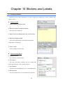
Chapter 10 Stickers and Labels
10-1 Editing Stickers
Stickers are used to add a description to a project. Stickers may display text as well as equations and
equation values.

Editing Stickers
1. Click on [Edit] in the Notes Area.
2. Enter the sticker in the Notes Window.
The typed text is displayed.
3. Select Text Color, Background Color, and Text Size.
4. Select the display method.
Select with/without border, with/without (transparent)
background, or non-display.
5. Click on [OK].
Click on [Apply] to check entry.

Sticker Characteristics
a. Displayed details
Text, equations, equation values
b. Text options
Text color, bold, italics, underline, text size, symbol font,
superscript, subscript, vector symbols, fractions
c. Text locations
Anywhere in the Graph Display Area, or in the Data Panel.
d. Miscellaneous
Text may be displayed over a maximum of ten positions.
59
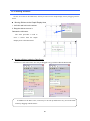
10-2 Moving Stickers
Stickers are created on the Data Panel, and may be moved to the Graph Display Area by dragging with the
mouse.

Moving Stickers to the Graph Display Area
1. Left-click and hold on the sticker.
2. Drag the sticker to move it.
Release the left button.
The same procedure is used to
move a sticker from the Graph
Display Area to the Data Panel.

Moving a Sticker Inside the Data Panel
A sticker or a title in the Notes Area may be dragged to any position within the Data Panel.
In addition to the Notes Area, a title may be moved up and down in any area in the Data
Panel by dragging with the mouse.
60
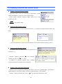
10-3 Displaying Equations and Equation Values

Equation Text and Equation Images
An equation expressed as text is referred to as „equation text‟, and its
actual representation is referred to as the „equation image‟.
In the scientific calculator example at right, „Sqrt(1-x^2)/4‟ is the
equation text, and
1  x 2 is the equation image.
4

Displaying the Equation Image
Enclose the equation text in half-width curly brackets ({ }) to display the equation image in stickers and
labels.
☆ To create equation text, simply create the equation in the scientific calculator, and copy the text.

Displaying the Equation Values
The equation values are displayed when the equation text is
enclosed in „!{}‟.
Example: {Sqrt(2)} represents
represents the value of
2 , and !{Sqrt(2)}
2 (i.e. 1.4142).
In addition to constants, equation values including
parameters and point coordinates may be displayed.

Number of Decimal Places Displayed
Equation values are displayed in floating point values of up to five significant digits. The number of
significant digits is changed by adding „| number of significant digits‟ to the equation.
Example: !{Sqrt(a)|8} displays the value of
a as an eight-digit floating point value.
61
10-4 Displaying Changing Equations

Displaying Equations With Changing Coefficients
When the values of parameters a and b are
provided, the function equation including these
parameters may be displayed using stickers. For
example, y  3x  2 is displayed if a = 3 and b
= -2 in the equation y  ax  b .
If the equation {y=ax+b} is entered in a
sticker, the equation y  ax  b is displayed.
{y=!{a}x+!{b}} is used to display the values a
and b. The „+‟ before !{b} is automatically
converted to „-‟ in accordance with the value of
b.

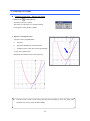
Displaying Polynomial Expressions
Polynomial expressions of six dimensions or less may be simply
displayed.
For example, ?{} is used to display the expansion of the
function 2( x  1)3 .
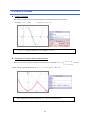
The diagram below shows the graph of the quadratic function y1  path ( x, P, Q, R ) passing through
the three points P, Q, and R, and the equation.
y
R
P
Q
O
x
62
10-5 Text Options


Bold, Italics, Underline
Bold
Text enclosed within <B> and </B> (or <b> and </b>) is displayed in bold.

Italics
<I> and </I>

Underline
<U> and </U>

Text Size

Large text
<L> and </L>

Small text
<S> and </S>

Superscript text
<Sup> and </Sup>

Subscript text
<Sub> and </Sub>

Colored Text
Six colors (black, blue, green, red, purple, grey) are available for colored text.
Text enclosed within <text color> and </text color> is displayed in the specified color.
☆ Any color may be specified using <color = #rrggbb> and </color>. rrggbb are the hexadecimal
values for the three primary colors. For example, red is specified with FF0000, and yellow with FFFF00.

Returning to the Original Format
The original format is restored with <Normal>.

Vector Symbols
<V> and </V> Same as v{ text string }.

Symbol Font Format
<Symbol> and </Symbol>

Used for Greek lettering etc.
Fractions
<Frac> - / - </Frac>
63
10-6 Displaying Multiple Stickers

Displaying Multiple Stickers
Insert two or more lines of consecutive spaces at the point at which the text in the sticker is to be
split.
☆ Sticker background color and display method cannot be selected for individual stickers.
☆ Overall text size and text color cannot be selected for individual stickers. Use the Text Options above
to select text color for each sticker.
☆ Up to ten stickers may be displayed.
10-7 Labels
As with stickers, text strings and equations may be displayed if the labels for basic graphic elements, curves, and
linked graphic elements are used.

Changing Label Text
Overwrite the label text.

Text Options and Equations
Text options and equations may be entered in the same format used
with stickers.
64
10-8 Notes
When you want to create a short document while creating a GRAPES project, select [Notes].

Editing Notes
1. Click on [Edit] in the Notes Area.
2. Click on [Note] in the Notes Window.
3. Enter the required text.
4. Click on [OK].
The entered text is saved to a file. However it is not
displayed on the screen as with stickers.
65
10-9 Font Configuration
After GRAPES 6.70, Sticky and Script can be dealt with without depending on kinds of
languages. However, most fonts correspond to only limited languages except for a few kinds
of Unicode font. For this reason, here users can select the font.
To Show Font Setting Window
Click on the option button of area palette to show the
option window, and then click on “Font” tag.
To Configure Fonts for Editing
Select a font for editing Sticky, Note and Script
To Configure a Font for Sticky
You can select different fonts for Alphanumeric
characters and for Other characters

Return to Default of Fonts
If you click on “Default”, the regular font of the system for editing, Times New Roman for
Alphanumeric characters, MSP Gothic for Other characters of Sticky, will be set
respectively.
Since the fonts configured here are recorded in each user‟s registry when finishing GRAPES, you can
use it with same configuration next time. However, the change of configuration is not recorded in
respective project file.
66
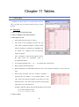
Chapter 11 Tables
11-1 Data Input
GRAPES provides a 200 row x 10 column table. Values in
cells in the table may be referenced from functions outside
the table.

Data Input
1. Click on [Edit] in the Notes Area.
2. Click on [Table] in the Notes Window.
3. Enter data in a cell.

Only numerical values may be entered.

The results of the calculation become the cell
value when a function equation is entered. Only
function equations recognized by GRAPES may
be entered. See „Equation Text and Equation
Image‟ for details.
The y coordinate is entered in the adjacent cell to
the
right
when
the
calculation
result
is
two-dimensional data.

Text strings beginning with „ // ‟ or „ ” ‟ are displayed as comment text.

Data is deleted with the [Del] key.

Double-clicking in the Edit Mode allows the use of the scientific calculator to enter values in
cells.

When using functions and the scientific calculator, „z‟
represents the row number, „w‟ the column number, „x‟ the
value of the cell in the first column of the same row as the
edited cell, and „y‟ the value of the cell in the second column
of the same row as the edited cell.
Example: When the edited cell is the third column of the second
row as in the diagram at right;
z  2 , w  3 , x  2.5 , y  6
4. Click on [OK].
67
Click on [Apply] to check entry.
☆ Table data is not entered until [Apply] or [OK] are clicked. When an existing graph references table
data, the graph is not updated until these buttons are clicked to change the data.
68

Batch Calculations
Batch calculations are executed for the selected area.
1. Click on the equation entry window at the top of the table to enter a function equation.

In the equation, „z‟ represents the row number for each
cell in the block, and „w‟ represents the column number.
Furthermore, „x‟ represents the value of the cell in the
first column of the same row as each cell, and „y‟
represents the value of the cell in the second column of
the same row.

Cells(row,column) is used to reference other cells.
2. Click on the

[Batch Calculation Example]
button (Calculate).
Calculation progresses in the row direction from top-left
to bottom-right of the selected area.

The y coordinate is entered in the adjacent cell to the
right when the calculation result is two-dimensional data.

When calculation is complete, the edited cell (selected
area) is immediately below the selected area.

Moving the Edited Cell
[Batch Calculation Example]

Move with the cursor.

Move to the right cell with the [Tab] key, and to the left cell with the [Shift]+[Tab] keys.

Move to the cell below with the [Enter] key.

Move to the desired cell by clicking with the mouse.
69
11-2 Editing Tables

Selecting Rows and Columns
Click on the row and column numbers.
Click on the cell at top-left to select the entire table.

Selecting Blocks
Drag with the mouse, or move with the [Shift]+cursor keys.
☆The mouse cannot be used for block selection when the cell is in the Edit Mode. In this case, press the
[ESC] key to clear the Edit Mode.

Moving Row and Column Data
Drag the row and column numbers.

Copy and Paste
Select from the right-click pop-up menu.

Shortcut keys (copy with [CTRL]+[C], cut with [CTRL]+[X],
paste with [CTRL]+[V]) may also be used.



Copy and paste with Excel spreadsheets is also possible.
Undo
Click on the
button (Undo).
Change Column Width
Drag the boundary of the top-most cell.
70
11-3 Using Table Data


Reading Data
Cells(row,column): Value of specified cell
Both constants and equations may be assigned to rows and columns.
An error value is returned if an invalid cell location, or a cell with no value, is specified.
Cell values are real numbers or error values.

CellsP(row, column)
：
Vector consisting of values of an assigned cell and of the
right-hand side cell.

Creating Scatter Diagrams
Draws a scatter diagram within x and y coordinates in two rows of
table data.
1. Select the range of cells to be graphed.
2. Click on the
button (Scatter chart).
The Create Scatter Diagram Window is displayed.
3. Remove the check for Point Sequence or Broken Line as
necessary.
A graph is drawn only if at least one is selected.
The data range selected in 1. above may be changed here if
necessary.
4.
Specify
the
graphic
element name.
The element is drawn
using Point Sequence in
Curve.
5. Click on [OK].
The Curve Property Screen
is displayed.
6. Set point and line color and thickness, and click on [OK].
☆ A graph created in this manner references a table, however table
71
data currently being edited is not reflected in the graph. Click on
[Apply] at the bottom of the Notes Window to ensure that data
currently being edited is reflected in the graph.
72
11-4 Scripts and Table Data
The use of scripts allows substitution of series of calculation results (e.g. number sequences)
in cells.

Substitution in Cells
Cells(row,column) := equation (both constants and equations may be entered in rows and
columns)
Example: Cells(1,2) := 4
☆When the value at right is two-dimensional data, the values are substituted in the specified cell and the
adjacent cell to the right.
For example, Cells(1,2) := (4,5) produces the same results as Cells(1,2) := (4) and Cells(1,3) := (5).
In case the value at right is two-dimensional data, it is also possible to use CellsP(row,
column)=equation.

Initialize All Cells
ClrAllCells
Deletes values in all cells in the table.

Samples
Substitute the 1st to the 20th items of a Fibonacci sequence in a cell.
Cells( 1 , 1 ) := 1
Cells( 2 , 1 ) := 1
For n := 3 to 20
Cells( n , 1 ) := Cells( n1 , 1 ) + Cells( n2 , 1 )
Next
The column number may be omitted in Cells(row,column). In this case, the column number is
assumed as 1.
Cells(row) = Cells(row，1)
If this format is used, the script above is as follows.
Cells( 1 ) := 1
Cells( 2 ) := 1
For n := 3 to 20
Cells( n ) := Cells( n1 ) + Cells( n2 )
Next
73
See „Chapter 14 Scripts‟ for further details.
74
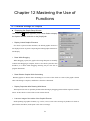
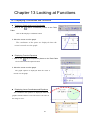
Chapter 12 Mastering the Use of
Functions
12-1 Detailed Settings for Graphs

Displaying the Graph Setup Window
Click on the
button (Options) on the Area Pallet to display
the Options Window, and click on the [Graph] tab.

Display Linked Graphic Elements
If a check is placed in this checkbox, the linked graphic element is
not displayed if one or points comprising the linked graphic element are
non-display.

Draw While Dragging
When dragging a point, the graph referencing that point is normally
redrawn after dragging is complete, however if a check is placed in this
checkbox, it is drawn while dragging. Drawing may be slow due to
program limitations.

Draw Relation Graphs While Calculating
Relation graphs are drawn while calculating to save time. If this check is removed, the graph is drawn
when calculating is complete, and flicker is therefore eliminated.

Display Properties After Drawing With Mouse
The Properties Screen is opened by default when drawing by dragging points and line segments with the
mouse. If this check is removed the screen remains closed.

Leave an Image of the Inside of the Graphic Element
Inside painting of graphic elements (e.g. circles, curves) is not left as an image by default. If a check is
placed in this checkbox, inside paint is also left as an image.
75

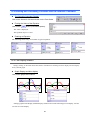
Calculated Density of Relations
With most relations, the function values for all points in the graph display area are investigated to draw
the graph. Some functions require considerable time for calculation, and the density of points in the
calculation is therefore reduced. See „4-4 How to Draw Relations‟.
1/1
1/2
1/4
1/8
▲ Graph of sin x  sin y  sin 3x  sin 3 y

Methods of Dawing Eplicit Functions
Function graphs are drawn by calculating the value of y in relation to x. When drawing the graph, it is
possible to select whether to draw a graph joining all these points, simply plot the points, or join the points
only under a given set of conditions.
Connect

Auto
Plot
Afterimage Density
By default, afterimages and locuses are displayed in a lighter shade of the graph color, however the
shade may be changed.
100%

75%
50%
Line Edge Processing
The shape of the end of the lines may be specified
when a graph is drawn with dotted or broken lines.
76
25%
0%
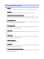
12-2 Detailed Settings for Functions

Displaying the Function Setup Window
Click on the
button (Options) on the Area Pallet to
display the Options Window, and click on the [Function]
tab.

Allow Negative Radius Vector
Normally the number of polar equation radius vectors and
circle radii of 0 or greater, however allowing negative radius
vectors and radii has many advantages.
Negative radius vectors and radii are allowed at initial setup,
however this may be changed.

Handle Vectors as Complex Numbers
When a check is placed in this checkbox, vectors are
handled as points on complex number planes. See „9-7 Vectors
and Complex Numbers‟ for details.

Θ in Defined Functions and Relations Handled as
Anglular Displacement
θ in relations and defined functions is expressed as angular displacement of the point (x,y). Note that θ
functions as a parameter in functions and basic graphic elements. Remove this check to handle θ as a
parameter in both relations and defined functions.

Handling of log
The user is able to select whether the log function is handled as a natural logarithm, or as a common
logarithm. Set as a natural logarithm at initial setup. The log function is not available in the scientific
calculator, however the natural logarithm function ln is available.

Angular Units
The user is able to select whether angles are handled with the circular method or the frequency method.
This selection affects trigonometric functions, inverse trigonometric functions, and the arg function. The
circular method is selected at initial setup.

Range of Angles
Returns the range of the angles obtained with inverse trigonometric functions and the arg function. Set
to 0    2 at initial setup.
This setting also affects display of the linked graphic element „angle‟. When the range of the angle is
      , „angle‟ always displays the minor arc.
77

Definite Integral Function  (integration variables, top limit, bottom limit, equations) Partition
Size
Definite integrals employ the 4th order approximation equation. This approximation equation does not
result in logical errors in up to and including 9th order polynomial expressions, and its application to
smaller individual sections of the integral partition allows for very high calculation accuracy for general
functions.
78
12-3 GRAPES Functions

Left Functions
Arguments are normally on the right-hand side of the function. The parentheses indicating the range of
the arguments may be omitted with trigonometric functions and logarithmic functions. For example,
sin( 2 x ) may be written as sin 2 x . Other functions require that the range of the argument be expressed
clearly in parentheses.

sin x , cos x , tan x : Trigonometric functions

A sin x , A cos x , A tan x : Inverse trigonometric functions
Angular units for trigonometric functions and inverse trigonometric functions are set to the circular
method at initial setup. The circular method or the frequency method may be selected under the [Function]
tab in the Options Window.

exp( x ) ： e x

log x : Natural logarithm or common logarithm
Set to natural logarithm at initial setup. Change to the frequency method under the [Function] tab in the
Options Window.

log( a, x ) : Log x with base a.

ln( x ) : Natural logarithm

sinh x , cosh x , tanh x : Hyperbolic functions

x ， 3 x : Square root, cube root, (entered from keyboard as „sqrt‟ and „cbrt‟).

int( x ) : Integer portion (equivalent to Gauss symbol)

round(x) : Rounding

frc(x) : Fraction frc(x)  x - int(x)

|x| or abs( x ) : Absolute value („| |‟ entered from keyboard as „[ ]‟)

unit ( x) ：Sign

rnd ( x ) : A random integer of 0 or greater and less than x.
Note that a random real number between 0 and 1 is returned when x = 1.

( x ) , ( x, y ) : Gamma and Beta functions

f ( x ) , g ( x ), h( x ), f 1( x )～f 5( x ) : Defined functions

f ' ( x ) ～f 5 ' ( x ) : Derivatives of defined functions.

f ' ' ( x ) ～f 5' ' ( x ) : 2nd derivatives of defined functions.

F ( x )～F 5( x ) : Indefinite integrals of defined functions. F ( x )   f (t ) d t
x
0
th
Note that f (x ) is limited to up to and including 8 order polynomial expressions.

nCr( x,y ) : Binomial coefficient
79

gcd( x,y ) ， lcm( x,y ) : Maximum and minimum common multiples.

f ( x, y ) ， f ( x , y , z ) ， f ( x, y , z , w) : Defined functions (similar to g , h, f 1 ～ f 5 )

Max ( x1 ,  , xn ) , Min( x1 ,  , xn ) : Maximum and minimum values.
Up to 20 arguments may be used, separated by commas.

Cells(m, n): Read table data. The value in the cell at row m and column n.
An error value is returned if an invalid cell location, or a cell with non-numerical data, is specified.
The value of the first column is returned if the column number is omitted. Cells(m) = Cells(m,1)

rgb ( r, g , b) : Returns a 24-bit integer color value.
r, g, and b are real numbers between 0 and 1 representing the strength of red, green, and blue.
Example: rgb(1,0,0) represents red, rgb(1,1,0) represents yellow, and rgb(0.5,0.5,0.5) represents gray.

hsl( h,s, l ) : Returns a 24-bit integer color value.
h, s, and l are real numbers between 0 and 1 representing hue, chroma, and
brightness.
The function is periodic for h. hsl( h+1 , s , l ) = hsl( h , s , l )
Example: hsl(0,1,0.5) represents red, hsl(0,1,0.8) represents light red, and hsl(0,0,0.5) represents
gray.
0

1
h
1
1
s
l
0
0
area(x): Display area
Top-left of the display area is ( area (1) , area (3) ) , bottom-right is ( area ( 2) , area ( 4) ) .

Pressed(virtual key code): Checks whether or not the specified key has been pressed.
True (1) if the key returned with the virtual key code has been pressed, and false (error value) if not.
The virtual key code is an integer defined in the Window system.
80
12-4 Special Functions

Right Functions
Functions in which the function symbol is placed after the argument.

x !: Factorial

x  : Converts frequency to radians („º‟ entered from keyboard as „degree‟).

.x , .y: x and y components of a vector.

.r: Circle (basic graphic element) radius


Functions Without Arguments
y1～y 20 : Function values (may only be referenced from within explicit and relations)

P , Q etc.: Points

O: Origin

X: Variable sets (x , y)

r ,  : r  len ( x, y ) ，   arg( x, y )


(usable only within relations and defined functions)
Functions and Functions and Parameter Notation as Arguments
sol ( f ( x )  g ( x ) , n ) : Within the solutions to a 4th order or lower equation f ( x )  g ( x ) ,
returns the nth from left of the real number parts in order of smallest to largest ( n  1, 2, 3, 4 ).
n  1 when n is omitted.

cof ( n , f ( x )) : Returns the nth coefficient when f (x ) is a 6th order or lower polynomial.
Example: cof(2 , ( x  2) 3 )  6

(parameter, initial value, final value, equation): Sum of sequence of numbers („‟ entered
from keyboard as „sum‟).
5
Example: If
k
2
,  ( k ,1, 5 , k 2 ) .
k 1
An equation including the variable x in the initial or final value cannot be substituted.

parameter, initial value, final value, equation): Product of sequence of numbers („‟
entered from keyboard as „product‟).
An equation including the variable x in the initial or final value cannot be substituted.

 (integration variable, bottom limit, top limit, equation): Definite integral („ ‟ entered from
keyboard as „igr').
Example: If


0
sin 2 x dx ,
 ( x , 0 , , sin 2 x ) .
Parameters and x are used as the integration variable.
81
An equation including the variable x in the upper or lower limit cannot be substituted.

Step(parameter): Range of increase/decrease for parameter.
82
12-5 Vector Functions

Real Number Value Functions

path ( x , P1 ,  , Pn ) : An ( n1 )th function passing through the provided n number of points.

| P | or len ( P) : Vector size („| |‟ entered from keyboard as „[ ]‟).

len( P1 , P2 ) : Distance between two points.

arg( P) : Angular displacement (the range of the angle is set in [Function Setup]
( 0  arg  2 ,    arg   ).

arg( P1 , P2 ) : Angle P1OP2
arg( P1 , P2 , P3 ) : Angle P1 P2 P3 forming three points.

det(a, b, c, d): Determinant value a d  b c
det( P , Q ): Determinant value P.x  Q.y  P.y  Q.x

perp(P , A, B) ：Length of perpendicular line drawn from point P to straight line AB（length of
perpendicular line entered from keyboard as „perp‟）

Crad(A, B, C): Radius of the circumcircle of the triangle ABC („circumcircle radius‟
entered from keyboard as „crad‟).

Irad(A, B, C): Radius of the incircle of the triangle ABC („incircle radius‟ entered from
keyboard as „irad‟).

Vector Value Functions

roll( t ): Returns points (cos t , sin t ) on the unit circle.

P(n): Coordinates of the nth point (points P, Q, …, V, A, …,N are numbered 1, 2, 3, …,
21).
This function is used only in stickers and labels.

unit ( P ) : Unit vector in the OP direction.

gcentr(A, B, C): Center of gravity of the triangle ABC („center of gravity‟ entered from
keyboard as „gcentr‟).

ccentr(A, B, C): Circumcenter of the triangle ABC („circumcenter‟ entered from keyboard as
„ccentr‟).

hcentr(A, B, C): Orthocenter of the triangle ABC („orthocenter‟ entered from keyboard as
„hcentr‟).

icentr(A, B, C): Incenter of the triangle ABC („incenter‟ entered from keyboard as „icentr‟).

ecentr(A, B, C) ：Excentre of triangle ABC (“Excentre entered from keyboard as „ecentr‟)
Other excentres are ecentr (B, C, A) and ecentr(C, A, B)
83

intr(A, B, C, D): Intersection of the two straight lines AB and CD („intersection‟ entered from
keyboard as „intr‟).

intr( A , B , C , r ): Intersection of the straight line AB and the radius r from the center C.
The other intersection is intr(B, A, C, r).

intr ( A , a , B , b ): Intersection of the radius a from the center A and the radius b from the
center B.
The other intersection is intr (B, b, A, a).

perp ( P , A , B ):
Base of the perpendicular line from the point P to the straight line AB („base
of the perpendicular line‟ entered from keyboard as „perp‟).

mid( P , Q , m , n ): The point dividing the line segment AB into m : n.

rot( P ):
Rotate point P around the origin by angle 90º („rot‟ entered from keyboard as
„rot‟).

rot( P, t ): Rotate point P around the origin by angle t.

rot( P, C, t ): Rotate point P around point C by angle t.

polygon( t , P1 , P2 ,  , Pn ) : A point on an edge of a polygon of n angles. One revolution of
the polydon with 0  t  n ( n  20 ).

proj( x, y , z, s, t , d ) : Returns the coordinates of a point in space ( x, y , z ) when projected
onto a flat plane.
s, t, and d are the plane angle, the solid angle, and the distance from the origin to the viewing point.
Parallel projection if d  0 or d is omitted.

See „9-6 Defined Functions and Vectors‟ for the relationship between defined functions and
vectors.
84
12-6 Operators and Variables

Operators

＋，－，×，／: Four arithmetical operators

＾: Square of a real number
x^ y  xy
If x  0 , a value results only if y is an integer.
Interpreted as the square of the function when placed immediately after a trigonometric function
(e.g., sin n x  (sin x) n ）.

x mod y : Integer remainder

 ,  ,  ,  ,  ,  ” Comparison operators
These operators return 1 if true, and an error value if false.
The graph is not drawn if the function value is an error value.
For example, for y  x ( x  0) , the graph is drawn only within the range x  0 .

AND, OR, NOT: Logical operators
These operators return 1 if true, and an error value if false.

Vector Operators

＋，－: Vector addition and subtraction

・: Vector dot product

×: Real number x vector (x may be omitted)

／: Vector / real numbers


Parameters
a,b,c,d,k,m,n,p,q,s,t,u,v,
 is handled as a function expressing angular displacement with relations and defined functions.

Variables

x, y, z, w: z and w are used only with defined functions and scripts.

: Angular displacement for polar equations (used only with relations and defined functions).

X: Represents the point ( x , y ).

Y: Represents the point ( z , w ) (used only with defined functions and scripts).

Constants

e : Natural log base

 : Circle ratio
85
12-7 Evaluation Priority Sequence

Priority Sequence

The part enclosed in parentheses is evaluated first.

Functions and operators are evaluated in the following priority sequence.
1. Right functions
2. Exponent
3. Multiplication with the multiplication symbol omitted
4. Left Functions
5. Multiplication and division
6. Addition and subtraction
7. Comparison operators, logical operators (AND has priority over OR)


Evaluated from left of the equation in all other cases.
Functions in Which Arguments are Not Enclosed in Parenthesis
Arguments for the following functions must be enclosed in parentheses.
sin , cos , tan , Asin , Acos , Atan , log ,
,3
The range of the arguments for these functions is determined as follows.

Until an arithmetic operator, logical operator, comparison operator, space, or left function is
encountered.
Example: sin a cos x 2  1  (sin a)(cos x 2 )  1
s i an( x  1) 2  1  s ian( x  1) 2   1
sin a ( x  1) 2  1  (sin a)( x  1) 2  1

All up to an exponent symbol placed immediately after a trigonometric function is handled as
a single function.

Right functions and exponent arguments are limited to immediately previous notation, values,
and parentheses.
Example: 2n !  2 (n ! ) , 2 a x 2  2a( x 2 )
☆ Add parentheses, or delineate with spaces, if priority relationships are unclear.

Displaying the Range of Functions Arguments
The above rules are in daily use, however they tend to be vague.
The manner in which GRAPES makes evaluations may be verified with
the scientific calculator.
86
Click on the
button (Scientific Calculator Argument Display Range).
The range of the argument is displayed with a green boundary.
87
12-8 Function Input Examples
(1) y  2 x3  4 x 2  x  2
(2) y  1  2 x
2x
3
← Insert a space between 2 / 3 and x.
(4) y  log 2 ( x  1)
(3) y  2 x  5
(5) y  2 x  4 x  x  2
3
2
x
(6) y  e 2 sin 4 x
88
12-9 Limits to Domains

Limits to Domains
The domain is placed after the function equation to limit the domein of the function.
Example: y  x 2 ( x  0)
，
y  sin x ( t  x  t  1 )
t  x  t  1 may be written as (t  x ) and ( x  t  1) .

Synthesis of Functions with Limited Domains
 x 2 ( x  1)
, they are
2  x ( x  1)
When two or more functions with limited domains are combined as in y  
joined with the logical OR operator as in y  x 2 ( x  1) or (2  x)( x  1) .
The example above may be written as y 3  y1( x  1) or y 2( x  1) .
89
12-10 Derived Functions and Indefinite Integrals
To use differentiation and integration in GRAPES, first register the target function as a defined function,
and use the derived function and indefinite integral.

Using Derived Functions
1. Register the function to be differentiated as a defined function.
Register the function for differentiation as a defined function.
For example, as f ( x)  x 2  2 x .
2. Use the derivative of the defined function to write the graph equation.
Use the derived function (e.g. f ' , g ' , h ' ) of the defined function to write the equation.
For example, y 2  f ' ( a )( x  a )  f ( a ) .
☆ First and second derivatives may be used.

Using Indefinite Integrals
Eighth and lower order integer functions may be integrated. Use the Definite Integral Window and
definite integral functions for integration of other functions.
1. Register the function to be integrated as a defined function.
For example, f ( x)  x 2  2 x .
2. Use the integral of the defined function to write the graph equation.
Use the integral function (e.g. F, G, H) of the defined function to write the equation.
F ( x ) is expressed as

x
0
f (t ) d t .
90
Chapter 13 Looking at Functions
13-1 Displaying Coordinates and Functions

Displaying Graph and Locus Coordinates
1. Click on the
(Show Coordinates) button on the Tools
Pallet.
Click on the Display Coordinates button.
2. Move the cursor over the graph.
The coordinates of the point are displayed when the
cursor is moved over the graph.

Displaying Function Equations
1. Click on the
(Show Expression) button on the Tools Pallet.
Click on the Function Equation button.
2. Move the cursor over the graph.
The graph equation is displayed when the cursor is
moved over the graph.

Displaying Locus Coordinates and Equations
The coordinates and equation are displayed with basic
graphic elements and locii even if the cursor is moved over
the image or curve.
91
13-2 The Function Values Window
The function value for the x value in functions and any desired function equation is displayed in the
Function Values Window, allowing multiple function values to be compared while viewing graphs.

Displaying the Function Values Window
1. Click on the
(Show Value of Function) button on the Tools Pallet.
The Function Values Window is displayed. The perpendicular line
indicating the x value is displayed in the Graph Window.

Changing the x Value (calculator input)
1. Click on the x Value Window.
2. Enter with the Scientific Calculator.
☆When x is provided as a numerical value, the x value may be changed
by dragging with the mouse as shown below.

Changing the x Value (drag with mouse)
Drag the perpendicular line in the Graph Window.
☆As shown below, when x is provided as an equation, it can not
be moved by dragging with the mouse.
Change the value
by dargging

Changing the Function Equation
1. Click on the function equation display
section.
2. Enter the equation with the Scientific
Calculator.
92
13-3 The Definite Integral Window
Definite integral values for functions are displayed in the Definite Integral Window. The integration area is
displayed on the graph.

Displaying the Function Values Window
Click on the
(Show Values of Definite Integral) button on the Tools Pallet.
The Definite Integral Window is displayed. Two perpendicular
lines indicating the range of integration are displayed in the Graph
Window.

Definite Integral Window
The Definite Integral Window displays the range of the definite integral, the
[Show] button, the [Diff] button, and the definite integral values. The [Select
Integrate/Area] button and the [Division] box are displayed at the bottom of the
window.
The integration areas are displayed in blue for positive, and red for negative.
The parameters may be manipulated (e.g. increased or decreased) while the
Definite Integral Window is displayed.

Changing the Top and Bottom Limit Values (calculator input)
1. Click on the box displaying the top and bottom values.
2. Enter with the Scientific Calculator.
☆ When the top and bottom limits are provided as numerical values,
change these values by dragging with the mouse as described.
93

Changing the Top and Bottom Values (drag with mouse)
Drag the perpendicular line in the Graph Window.
☆Drag the perpendicular line with the mouse as shown below, when the
top and bottom limits are provided as equations.

Displaying the Integration Area
Click on the button inside the [Show] border for the function to be displayed.

Displaying the Difference
Click on the button enclosed in the [Diff] border for functions for which the difference is to be
taken.
The integral of the difference with the function selected here is displayed for all functions. Place a check
in the bottom-most [Diff] button when the difference is not to be displayed.

Area and the Definite Integral
Click on the
button (Definite Integral) to find the value of the definite integral.
Click on the
button (Area) to integrate with the absolute value applied to the function value.
94

Number of Partitions for Approximations
Definite integrals are calculated with a special 4th order approximation equation. No errors occur with
up to and including 9th order polynomial expressions. Beyond this, the integration space is finely divided
for calculation. The number of partitions is a natural number of 200 or less.
95
13-4 Entering and Calculating Functions With the Scientific Calculator

The Scientific Calculator Display
Click on the Scientific Calculator button on the Tools Pallet.

Finding the Value of the Equation
Click on the
button (Calculate Equation).
The value is displayed.
The equation may be a vector.

Entering an Equation
The following shows entry of a number of typical equations.
13-5 The Display Switch
Simply clicking on the Data Panel label allows instantaneous switching between display and non-display
for any desired graph.

Graph Display and Non-display
Click on the graph label notation.
y
y
O
O
x
x
Setting a graph to non-display with the display switch to also sets the afterimage to non-display. Locuses
are also set to non-display.
96
13-6 Using the Background
Wallpaper images may be applied to the graph display area background.

Loading Background
Click on the
button (Paste Background).
Select the image file. bmp, jpg, or gif image formats may be used.

Applying the Background
Click on ▼, and then click on the
button (Paste).
The image on the clipboard is applied to the background. Note that the
image must always be copied to the clipboard first.

Stretching the Background
1. Click on the
button (Stretch Background Image).
Click again to undo the stretch.
Clicking on ▼ provides three types of stretch for selection.
Unchanged

Fit height
Stretchto Graph Window
Clearing the Background
Click on the

Fit width
button (Clear Background).
Saving the Background
When saving GRAPES data, only the loaded background file name is saved. The background is
therefore set when loaded only if the GRAPES save file and the background file are in the same folder.
Background applied from the clipboard is not saved.
97
Chapter 14 Scripts
14-1 What is a Script?
Scripts are small programs which run within GRAPES.

Script Characteristics

A control structure including repetitions and subscript calls.

Parameter control.

Substitution in graphic elements (point coordinates).

Substitution in table cells.

Calculation of various types of equations.

Control of drawing, display, and images.

Output of audio waveforms in accordance with function graphs.

Setting of conditions for automatic execution.

Script Editing and the Script Button
1. Click on [Edit] in the Notes Area.
2. Click on the [Script] tab.
3. Enter the script.
4. Click on [OK].
A button for the first line of the script appears in the Notes Area. This
button is referred to as the Script button.

Displaying the Script

The first line is displayed as the Script button.

When the first line includes a comment (//), the comment becomes the button title.

The script is not displayed if the first line includes the HideScript command.

Writing Scripts

Only one command may be entered per line.

Statements in the script are separated by a half-width space character.

Comments are preceded by a double-slash (//).

Statements used only in scripts (e.g. Draw) may be in upper or lower case.

Parameters are entered in lower case. Functions are entered as is (e.g. sin, Sqrt, Pi).

Multiple scripts (maximum of 30) are separated by blank lines.
98
14-2 Script Configuration Elements

Variables
In addition to parameters and basic graphic elements, x, y, z, and w are available as local variables.

Substitution
Equation values may be substituted in parameters, basic graphic elements, and table cells.

Conditional Statements and Control Structures
„if – then‟ and „if – then - else‟ for executiuon only while a certain condition is satisfied, „for - next‟ for
repeated execution, and „while – wend‟ for repeated execution only while a certain condition is satisfied.

Graph Drawing Control
Draw and OverDraw for calculation and drawing of graphs, Calc for calculation of coordinates, and
Refresh and RefreshSticker for updating displays and stickers.

Drawing Color Control
SetColor for changing the color of points and function graphs, SetLineColor for changing the color of
lines, and SetInnerColor for changing the paint color.

Image Control
ClrAImg for deleting images, SetAImg for creating images, and AImgOn and AImgOff for controlling
images.

Display Control
ShowObj for displaying graphs, HideObj for setting graphs to non-display, and InvShowObj for
switching graphs between display and non-display.

Display Range Control
SetArea for changing the display range.

Sound Output
Play, PlayAfter, and PlaySync for output of audio waveforms in accordance with function graphs, and
SetSampleRate for changing the sampling frequency.

Setting of Conditions for Automatic Execution
„on – change‟ for automatic execution of scripts when the specified function is rewritten, or when points
or parameter values are changed.
99

Execution Control
„SetTme – Wait‟ for setting wait time, Pause for pause until input, and „end‟ for terminating execution.

Execute Another Script
Another script may be executed with „Call‟. Up to four arguments may be passed to the called script.

Script Button Non-display
The Script button is not displayed if HideScript is placed at the start of the script.
14-3 Executing and Terminating Scripts

Execution With the Script Button
Click on the Script button to execute the script.
☆ An error message is displayed when the Notes Window is closed if the script contains a syntax
error. Note that checking for syntax errors is not comprehensive. An error message may therefore
not be displayed in the event of a syntax error.
☆ When an error occurs at runtime, the line containing the error is not executed and processing
moves to the next line.

Execute With the On change Instruction
When the first or second lines of the script contain the On Change command, the script is executed when
the specified element is changed.
Example: „On a, b Change‟ is executed when parameter a or b is changed.

Terminate Script
Continue pressing the F1 key.
Used to interrupt and terminate scripts requiring considerable time for execution before processing is
completed.
100
14-4 Variables and Substitution

Global Variables
May be used as variables within parameters, point coordinates, table cells, and scripts.

Local Variables
Four local variables (x, y, z, w) may be used. These variables are valid only within a script during
execution. For example, variable x in script A and variable x in script B are unrelated.
Real numbers and error values may be substituted in local variables. Use X and Y when handling
two-dimensional vector values with local variables. X is a variable set (x, y) and may therefore be written
X = (x, y). Similarly, Y = (z, w).
Example: X = (1, 2)
and
x := 1
y := 2
return the same result.
The initial value of a local variable is an error value which is discarded after execution. When a script is
called with the CALL command during execution of another script, the argument for the CALL statement
is substituted in these variables.
Example: If the following is written in a C language-like format,
//Sum
a := x+y
it appears as follows.
void Sum( x , y , z , w);
{a=x+y}

Substitution
Equation values may be substituted in parameters, point coordinates, table cells, and local variables x, y,
z, and w as follows.
Substitution object ;= equation
Leave a space between the substitution object and „:=‟.the same applies between „:=‟ and the equation.
If the equation has no value (e.g. 1/0) when substituting in parameters and points (coordinate
component), the substitution statement is not executed.

Parameter := equation
Example: a := sin t
101

Point (i.e. the point coordinate component) := equation
Example: P := (2,3) ，P.x := 2
☆ Speed of execution is slower with substitution in points.
For example, rather than using;
P := (2,3)
it is much faster to used P(s,t)
s := 2
t := 3

P（point number） := equation
Point numbers are 1, 2, 3, …, 7 , 8, 9, …, 21 for P, Q, R, …, V, A, B, …, N.
Example: P(2) := (2,3)
(same result as Q := (2,3)）
P(n) := (2,3)

Local variable := equation
Example: x := tan t
☆ In addition to real numbers, local variables may also take error values. The substitution
statement is therefore executed even if the right of the substitution statement has no value, and
an error value is substituted.

Cells(row, column) := equation (in addition to constants, equations mayalso be substituted in
rows and columns)
Example: cells(1,2) := 4 / a
☆If the value on the right is two-dimensional data, the value is substituted in the specified cell
and the cell to its right.
Example: Cells(1,2) := (4,5) has the same result as Cells(1,2) := 4 , Cells(1,3) := 5.
☆The cells in the first column are displayed if the column number is omitted.

CellsP(row, column) : = equation（For row and column, you can enter an equation besides
regular number）
When the right-hand side is vector data, the value is substituted in the specified cell and the
cell to its right.
When the right-hand side is not vector data, the value is not substituted.

ClrAllCells
Clears the values in all cells in the table.

Inc and Dec
Inc/Dec increments/decrements the parameter or local variable value by the specified amount.
102
Inc(parameter, increment)
Dec(parameter, decrement)
When the increment/decrement is 1, the increment/decrement may be omitted (i.e. „Inc(a)‟).
103
14-5 Control Structures and Conditional Statements

for - next
The for - next statement repeats execution of the statements between „for‟ and „next‟.
for „parameter or local variable‟ := „initial value‟ to „final value‟ „step‟
executable statement (multiple lines possible)
next
When „step‟ is omitted, an increment of „1‟ is assumed.

while - wend
Repeats execution of the statement between „while‟ and „wend‟ while the condition is satisfied.
while „conditional expression‟
executable statement (multiple lines possible)
wend

if - then Executes the command if the condition is satisfied.
if „conditional expression‟ then „executable statement‟
As follows if commands extend over multiple lines.
if „conditional expression‟ then
executable statement (multiple lines possible)
end if

if - then - else Executes the first command if the condition is satisfied, and executes a different command if the
condition is not satisfied.
if „conditional expression‟ then „executable statement１‟ else „executable statement2‟
or
if „conditional expression‟ then
executable statement (multiple lines possible)
else
executable statement (multiple lines possible)
endif
104
14-6 Drawing and Calculation

Draw
Calculates the coordinates in accordance with the current parameter values, and draws the graph.
Add a colon to Draw (i.e. „Draw:‟) to eliminate the locus.
The entire display, except for stickers, is updated.
☆ Substituting values in variables in a script does not result in recalculation of the graph. Draw and
Calc are used for recalculation.

OverDraw
Basically similar to Draw, except that a new graph is added to the screen, rather than the screen being
erased and redrawn. Faster than Draw.

Calc
Calculates the coordinates in accordance with the current parameter values, and saves the loci and image
in internal memory. Note that the screen is not updated. Use Draw or Refresh (described below) to update
the screen.
Add a colon to Calc (i.e., „Calc:‟) to eliminate the locus.
Since the graph is not drawn, Calc is faster than Draw and OverDraw.

Refresh
Calc leaves the image and results of loci calculation in internal memory, however the screen is not
updated. Refresh displays the image and locii left in memory with Calc in the Graph Window.
Refresh displays the image and locii, however it does not display the current graph. Use Draw to display
the current graph. Draw also displays the image.

RefreshSticker
Updates sticker display.
The current result is updated when an equation value is displayed in a sticker.
105
14-7 Changing Graph Color

SetColor(element name, color)
Changes the display color of a graphic element. Changes point color for basic graphic elements and
curves, graph color for function graphs, and line color for linked graphic elements.

Graphic elements may only be specified one-at-a-time.

Colors are specified in a 24-bit integer value representing RGB, however since GRAPES cannot
handle hexadecimal values, color is specified with the rgb and hsl functions.
Example: SetColor(y1 , rgb(0.8, 0, 1))
The function graph y1 is displayed in purple.

SetLineColor(element name, color)
Changes the display color of a graphic element. Changes line color for basic graphic elements and
curves, graph color for function graphs, and line color for linked graphic elements.

SetInsideColor(element name, color)
Changes the paint color for basic graphic elements, curves, and linked graphic elements.
14-8 Deleting and Creating Afterimages

ClrAImg(element name)，ClrAImg
Deletes the image and locii of a graphic element.
Note that ClrAImg is an abbreviation of „Clear After Images‟.

ClrAImg(element name) deletes only the image of the graphic element.

Functions, relations, curves, and basic graphic elements, as well as linked graphic elements may
be specified as the graphic element name. Multiple graphic elements are delineated with commas.
Example: ClrAImg(y1,C2,P,L2) deletes the images of the function y1, the relation C1, the graphic
element P, and the linked graphic element L2.

Use ClrAImg to delete all graphic element images without the need to specify graphic element
names.

SetAImg
Leaves images of all currently drawn graphs.
Inside colors of circles and rectangles are not left as images.
106
14-9 Display Control

AImgOn and AImgOff
Use of the AImgOff command ensures that, irrespective of the setting for the graphic element, no image
is recorded when the
button (Image OFF) in the Parameter Area is clicked. Returns to the original
status with the AImgOn command.


ShowObj(element name)，HideObj(element name)，InvShowObj(element name)
HideObj(element name)
The graph is no longer displayed when the graphic element display switch is clicked.
Functions, relations, curves, and basic graphic elements, as well as linked graphic elements may be
specified as the graphic element name. Multiple graphic elements are delineated with commas.
Example: HideObj(y1,C2,P,L2) does not display the function y1, the relation C1, the graphic element P,
and the linked graphic element L2.

ShowObj(element name)
Clears the clicked status of the graphic element display switch, and displays the graphic elements.

InvShowObj(element name)
Toggles graphic element display/non-display.

SetArea(x1,y1,x2,y2)
Displays the area having its diagonal between the two points (x1,y1) and (x2,y2) on the entire screen.
This command redraws all graphs.
107
14-10 Sound Output

Play(parameter, start seconds, finish seconds, waveform function)

Outputs sound digitized at a sampling rate of 22,050Hz.
Example: Play( t , 0 , 2 , sin880Pit) („Pit‟ is the product of  andｔ ) outputs a 440Hz sine wave for 2
seconds.

Provides vector data at stereo output.
Example: Play( t , 0 , 2 , (sin 880Pit , sin 882Pit)) outputs a 440Hz sound from the left channel and a
441Hz sound from the right channel.
All parameters used with GRAPES, and the variable x, may be used as parameters.
The performance begins after all data has been calculated. Functions may also be used as waveform
functions.

Play
The Play command requires no parameters, and plays the data remaining in the work memory.

Plays Wave data created with the PlayAfter command.

Replays the Wave data played last.

PlayAfter(parameter, start seconds, finish seconds, waveform function)

Wave data created with PlayAfter is placed in the work memory and is not played.

When the next PlayAfter command is executed while Wave data remains in the work memory,
the sets of data are joined.

The Play command is executed to play Wave data created in the work memory.

The play order may become confused in high performance PCs if multiple Play() commands are
executed in succession. In this case, create connected data with the PlayAfter command, and play
it with the Play command.
Example: PlayAfter( t , 0 , 1 , sin400Pit)
PlayAfter( t , 0 , 2 , sin600Pit)
Play
Output a 200Hz sine wave for 1 second, and a 300Hz sine wave for 2 seconds.
108

PlaySync(parameter, start seconds, finish seconds, waveform function)
The PlaySync command differs in only one point from the Play command.

Play with the Play command is conducted in the background, however with PlaySync, the next
command is not executed until play is finished.

SetSampleRate(sampling rate)
Changes the sampling rate.
Example: Set to 48,000Hz as follows.
SetSampleRate(48,000)
The new sampling rate is retained until GRAPES is terminated.

A set of Wave data may be played for a maximum time of 480,000/sampling rate (seconds).

Digitization is fixed at 16-bit. Since the interval -10 – 10 is mapped to -32768 – 32767 in
GRAPES, the sound becomes distorted if the waveform function value exceeds this range.

Saving Sound
The last played sound is saved to a Wave file.
Click on [Save Sounds] in the [File] menu.
109
14-11 Execution Control

SetTime(milliseconds) - Wait
SetTime sets a timer. Waits at the Wait position until the set time has elapsed. Processing moves
immediately to the next command when the set time has elsped. Specified in milliseconds.
Example: SetTime(n)
a := 3
Draw
Wait

//Processing waits n milliseconds after execution of SetTime.
Wait (milliseconds)
Halts processing for the specified time. Specified in milliseconds.

Pause，Pause(message)
Halts execution of a script and waits for input.
The message is displayed and processing is halted when Pause(message) is used.
Pause
Pause(Check point movement
Click on [OK] to continue or [Cancel] to halt processing.

Call(subscript name, argument 1, argument 2, argument 3, argument 4)
Executes another script in the same project. Control moves to the next line following execution.
The values of the four arguments of the Call command become the initial values of the subscript local
variables x, y, z, and w. All of these arguments, or consecutive arguments (e.g. last 3, 2, or 1 arguments),
may be omitted. Error values are substituted in omitted arguments.
Arguments must contain real numbers or error values. When a two-dimensional vector value is assigned
to an argument, it is assumed that two real number values have been assigned. For example, all of the
following have the same result.
Call(test , (1,2),(3,4))， Call(test , (1,2),3,4)， Call(test , 1,2,(3,4))， Call(test , 1,2,3,4)
110
Note that the following format is not permitted.
Call(test , 1,(2,3),4)

End
Terminates execution of a script. If the script being executed has been called from another script with the
Call command, control is returned to the calling script.

on element_name change
The script is executed automatically when the specified element is changed.

Parameters, basic graphic elements and curves (e.g., P, Q), defined functions, functions, and
relations may be specified. Linked graphic elements may not be specified. Multiple elements are
delineated by commas.

This command must be entered in the first or second line of the script.
Example: on a,b,f change
Executed when parameter a or b, or function f, is changed.
In the following example, when the value of parameter a is changed, parameter t is initialized, and the
image and locii are deleted.
//Initialize
on a change
t := 0
calc
ClrAImg

Scripts and Deletion of Afterimages
Afterimages are deleted after initializing parameter values. This is due to the fact that, since images are
recorded immediately before a new graph is drawn, the initial image cannot be deleted before the image for
the current graph created immediately before the next graph is drawn.

Execution Timing
Automatic execution with the on – change statement occurs only when the target element is changed
directly from the Data Panel. When an element is changed from the Data Panel, coordinates are
recalculated and the graph is drawn, however automatically executed scripts are executed immediately
after change from the Data Panel, and coordinates then recalculated and the graph drawn.
111
Chapter 15 Tips
15-1 Using Pop-up Menus

Data Panel Pop-up Menu
Right-click on the function equation display section of the
Data Panel.
The pop-up menu appears, and the function may be amended or
deleted, or the image deleted.

Sticker Pop-up Menu
Right-click on the sticker.
The pop-up menu appears, and the entire sticker may be edited, set to non-display, or deleted.
This operation is applied to all stickers, even when multiple stickers are displayed on the screen. For
example, all stickers are set to non-display if non-display is selected.

Graph Display Area Pop-up Menu
Right-click the Graph Display Area.
The pop-up menu appears, and various operations may be
applied to the graph.

Zoom
×10, ×5, ×2, ×1/2, ×1/5, ×1/10

Image operations

Set a point

Graph property display
The properties of the graph or graphic element at the clicked
position are displayed and may be edited.

Show of graph coordinates and expression

Capture and Print
112
15-2 Printing and Pasting Screens

Printing Screens
1. Click on the
(Print) button on the Toolbar.
The Print Screen Setup dialog appears.
2. Adjust the screen size.
Click on [Printer properties] under [Size of Paper] when changing
printer settings.
3. Select the print settings.
When [Graph (hi-res Color)] or [Graph (hi-res B/W)] are selected,
vector data is used to print smooth graphs.
When [Graph (capture)] is selected, the graph is printed at the screen
quality. When [Whole GRAPES] is selected, both the Graph Window
and the Data Panel are printed. Place a check in the [Adjust Print Size]
checkbox under [Size of Graph] for high-quality printing.
4. Click on [OK].

Copying the Screen and Pasting Into a Word Processor
Document
1. Click on the
(Capture) button on the Data Panel.
The entire Graph Display Area is copied to the clipboard. Click
on ▼ to the right of the Copy button to select the data
format and copy target.
2. Click on the [Paste] in the [Edit] menu of the
word processor.
The image data on the clipboard is pasted into the
document. See the word processor manual for
details on subsequent operations.
☆ Depending on the software used in pasting to the document when copying the screen, it may not be
possible to obtain sufficient screen resolution despite selecting [Graph (hi-res Color)] or [Graph (hi-res
B/W)]. In this case, click on the Copy key while holding down the Shift key.
113
15-3 Saving Screens and Sound

Saving the Graph Screen
Click on [Save Image] in the [File] menu.
Screens may be saved in Windows Bitmap (*.bmp), JPEG (*.jpg),
Enhanced Metafile (*.emf), and Windows Metafile (*.wmf) formats.
Enhanced Metafile and Windows Metafile formats permit saving of
high-quality graphs without jagged edges.

Continuously Saving the Graph Screen
1. Click on [Successive Save Images] in the [File] menu.
The [Successive Save] icon
appears on the Toolbar, and the screen
image is then saved each time the screen is updated.
2. Click on the
(Successive Save) icon.
The following example uses the file name „Image‟ for continuous save. The screen image is saved each
time parameters are changed. The text string beneath each screen image is the file name under which each
is saved.
Image000

Image001
Image002
Image003
Saving Sound
Saves the sound last played with the Play command in the script.
Click on [Save Sounds] in the [File] menu.
114
Image004
15-4 Customizing the Data Panel
The display sequence, and display/non-display, may be changed for each area of the Data Panel and for
each individual item of data.

Moving Each Area
Drag the area title part to another area.

Hiding Each Area
Select [Show Area] in the [View] menu, and click on the display/non-display area.

Moving Individual Equations and Data
Drag the Function Equation Window and Parameter Value Window up or down.
The data display sequence may be changed within the same area.
The linked graphic element and sticker display sequences can not be changed.
115

Hiding Individual Equations and Data
Right-click on the data to be hidden, and select [Hide Data].
Functions, graphic elements, and parameters may be hidden.
To re-display hidden data, select [Show
Data] in the [View] menu.

Fixing Parameter Values
Click on the parameter notation.
A parameter value cannot be changed while the label is selected.
Click again to free the value.
116
15-5 Use in Presentations

Presentation Mode
Displays equation images and parameter values in double-sized font.
Click on [Presentation Mode] in the [View] menu.
Click again to return to the original font size.
Normal Mode

Presentation Mode
Enlarging the Graph Display Area
Hide the Control Pallet, and enlarge the Graph Display Area.
Right-click on the Control Pallet, and click on [Auto-Hide
ControlPalette].
Move the cursor to the top of the Graph Display Area to display the Control Pallet.

Using Markers
1. Click on the
(marking Pen) button on the Tools
Pallet.
The Marker Pallet appears, and the cursor assumes the
shape of a marker.
2. Draw by dragging with the left mouse button.
Drawing continues while the left button is held down.
3. Delete the marker by dragging with the right mouse button.
4. Click on the
(Delete All Markers) button to delete all
markers.
117
15-6 GRAPES Specification

Specification

Functions
20

Relations
9

Basic graphic elements and curves

Curve apexes
Maximum 5000

Defined functions
8

Linked graphic elements
30

Parameters
14

Stickers (partition display)
10

Scripts
20

Tables
200 x 10 cells

Graph display size
Maximum 1600 x 1600 pixels

Afterimages
3000

Undo (functions)
50 actions

Undo (areas)
200 actions
21 (excluding origin)
118