Download Part II - Random Processes Goals for this unit: • Give overview of

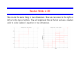
Part II - Random Processes
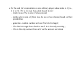
Goals for this unit:
• Give overview of concepts from discrete probability
• Give analogous concepts from continuous probability
• See how the Monte Carlo method can be viewed as sampling technique
• See how Matlab can help us to simulate random processes
• See applications of the Monte Carlo method such as approximating an integral or finding extrema of a function.
• See how Random Walks can be used to simulate experiments that can’t
typically be done in any other way.
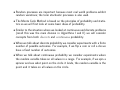
• Random processes are important because most real world problems exhibit
random variations; the term stochastic processes is also used.
• The Monte Carlo Method is based on the principles of probability and statistics so we will first look at some basic ideas of probability.
• Similar to the situation where we looked at continuous and discrete problems
(recall this was the main division in Algorithms I and II) we will consider
concepts from both discrete and continuous probability.
• When we talk about discrete probability we consider experiments with a finite
number of possible outcomes. For example, if we flip a coin or roll a die we
have a fixed number of outcomes.
• When we talk about continuous probability we consider experiments where
the random variable takes on all values in a range. For example, if we spin a
spinner and see what point on the circle it lands, the random variable is the
point and it takes on all values on the circle.
Historical Notes
Archaeologists have found evidence of games of chance on prehistoric digs, showing that gaming and gambling have been a major pastime for different peoples
since the dawn of civilization. Given the Greek, Egyptian, Chinese, and Indian
dynasties’ other great mathematical discoveries (many of which predated the
more often quoted European works) and the propensity of people to gamble, one
would expect the mathematics of chance to have been one of the earliest developed. Surprisingly, it wasn’t until the 17th century that a rigorous mathematics
of probability was developed by French mathematicians Pierre de Fermat and
Blaise Pascal. 1
1 Information
taken from MathForum, http://mathforum.org/isaac/problems/prob1.html
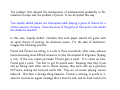
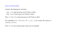
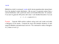
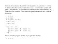
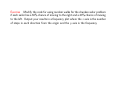
The problem that inspired the development of mathematical probability in Renaissance Europe was the problem of points. It can be stated this way:
Two equally skilled players are interrupted while playing a game of chance for a
certain amount of money. Given the score of the game at that point, how should
the stakes be divided?
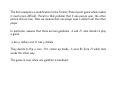
In this case “equally skilled” indicates that each player started the game with
an equal chance of winning, for whatever reason. For the sake of illustration,
imagine the following scenario.
Pascal and Fermat are sitting in a cafe in Paris and decide, after many arduous
hours discussing more difficult scenarios, to play the simplest of all games, flipping
a coin. If the coin comes up heads, Fermat gets a point. If it comes up tails,
Pascal gets a point. The first to get 10 points wins. Knowing that they’ll just
end up taking each other out to dinner anyway, they each ante up a generous
50 Francs, making the total pot worth 100. They are, of course, playing ’winner
takes all’. But then a strange thing happens. Fermat is winning, 8 points to 7,
when he receives an urgent message that a friend is sick, and he must rush to his
home town of Toulouse. The carriage man who has delivered the message offers
to take him, but only if they leave immediately. Of course Pascal understands,
but later, in correspondence, the problem arises: how should the 100 Francs be
divided?
How would you divide the 100 Francs? After we discuss probability you should
be able to divide the money and argue that it is a fair division.
What do we mean by probability and events?
• Probability measures the chance of a given event occurring. It is a number
between 0 and 1.
• The complement of an event is everything that is not in the event; for
example the complement of 3 or less hurricanes hitting Florida in 2011 is 4
or more hurricanes hitting Florida.
• If the probability of an event is 1 then it is certain to occur.
• A probability of 0 represents an event that cannot occur, i.e., is impossible.
• Probabilities in between 0 and 1 are events that may occur and the bigger
the number the more likely that the event will occur.
• “Rain tomorrow”, “crop yield”, “number of hurricanes to hit Florida’s coast
in 2011”, “ the number of times the sum of two dice thrown is even” are
all examples of events for which we may be interested in determining their
probabilities.
Notation & Terminology:
• Let X denote the random variable, for example the sum of two dice when
they are thrown.
• The set of all possible outcomes is denoted Ω. For example, if we roll one
die the possible outcomes are Ω = {1, 2, 3, 4, 5, 6}.
• We will denote an event as E. So for example, if we roll a single die and
want to determine the likelihood of the result being an even number, then
E = {2, 4, 6}; note that E ⊂ Ω.
• We are interested in determining the probability of an event and will denote
it p(E).
The sum of all probabilities for all possible outcomes is 1.
The probability of an event will be the sum of the probabilities of each
outcome in the event.
The probability of the complement of an event E will be 1 − p(E).
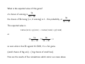
What is meant by the probability of an event?
Suppose the weather forecast is that the probability of rain tomorrow is 1/4=0.25.
We say the likelihood of rain is 25%. What does this mean?
The complement of this event is that there is NO rain tomorrow so the probability
of no rain is
1
1 − = 0.75
4
So there is a 75% chance of no rain tomorrow and thus it is 3 times more likely
that there is no rain tomorrow than there is rain.
Unions and Intersections
Consider the following two outcomes:
• A= { 3 or less hurricanes to hit Florida in 2011}
• B= { 4 or 5 hurricanes to hit Florida in 2011}
Then A ∪ B is { 5 or less hurricanes to hit Florida in 2011}.
The probability of A ∪ B is p(A ∪ B) = p(A) + p(B) because the events are
mutually exclusive.
Then A ∩ B is zero because both events can’t be satisfied.
Now consider two events which are not mutually exclusive.
• C = { rain tomorrow}
• D = { rain the day after tomorrow}
Then C ∪ D = { rain in the next two days} (i.e., rain tomorrow or rain the next
day).
Now the intersection of C and D is everything that is in event C and in event
D so
.
C ∩ D = { rain tomorrow and rain the next day}
What is the probability of C ∪ D? We can’t simply sum the probabilities. For
example if there was a probability of 1/4 each day (i.e., 25% chance) then we
can’t say there is a 50% chance that it will rain in the next two days. In the case
where the events are not mutually exclusive we have
p(C ∪ D) = p(C) + p(D) − p(C ∩ D)
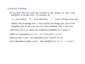
Conditional Probability
• If we know that one event has occurred it may change our view of the
probability of another event. For example, let
A = {rain today},
B = {rain tomorrow},
C = {rain in 90 days from now}
Assume that knowledge that A has occurred will change your view of the
probability that B will occur, but not of the probability that C will occur.
• We write p(B|A) to denote the conditional probability of B, given A.
• With our assumptions, p(C|A) = p(C) but p(B|A) 6= p(B).
• We say that A and C are independent, but A and B are not.
• For independent events A and C, the probability of p(A ∩ C) = p(A)p(C).
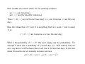
Example If we roll a single die (with sides 1, 2, 3, 4, 5, 6) what is the probability
that you will roll the number 4? If we roll two dice, what is the probability that
they will both be 4?
Clearly all numbers are equally probable and since the probabilities have to sum
to 1 and there are 6 possible outcomes, p(X = 4) = 1/6. To determine the
probability that a 4 occurs
on both dice, we note that they are independent events
1
so the probability is 16 16 = 36
.
Example Let’s return to the Fermat/Pascal problem of flipping a coin. We
know that heads and tails are each equally likely to occur. If heads occurs then
Fermat gets a point, otherwise Pascal gets one. When the game is interrupted
the score is Fermat 8 and Pascal 7. There is 100 francs at stake so how do you
fairly divide the winnings?
We first ask ourselves what is the maximum number of flips of the coin that
guarantee someone will win? Clearly Fermat needs 2 points and Pascal 3. The
worse case scenario would be for Fermat to get 1 and Pascal to get 3 so in 4
more flips we are guaranteed a winner.
If we determine the possible outcomes in these 4 flips then we can assign a winner
to each. Then Fermat’s probability of winning will be the number of outcomes
he would win over the total number of outcomes; similarly for Pascal. Then we
will know how to divide the money.
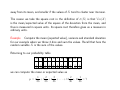
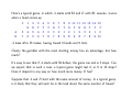
Here are the 24 possible outcomes for 4 flips and we have indicated the winner
in each case remembering that Fermat needs 2 heads to win and Pascal 3 tails.
HHHH (F)
HTHH (F)
TTTT (P)
THTT (P)
HHHT (F)
HTTH (F)
TTHT (P)
THHH (F)
HHTH (F)
HTHT (F)
TTTH (P)
THTH (F)
HHTT (F)
HTTT (P)
TTHH (F)
THHT (F)
So Fermat will win 11 out of 16 times so his probability is 11/16. Pascal will
win 5 out of 16 times so his probability is 5/16. Fermat should get 11/16 of the
money and Pascal the rest.
Simulating random processes using Matlab’s rand command
• Random events are easily simulated in Matlab with the function rand, which
you have already encountered. A computer cannot generate a truly random
number, rather a pseudorandom number, but for most purposes it suffices
because it is practically unpredictable.
We have seen that if you use the command x=rand() you get a number
between 0 and 1. It can also generate row or column vectors. For example,
rand(1,5) returns a row vector of five random numbers (1 row, 5 columns)
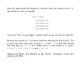
such as
0.2416 0.9644 0.4519 0.3278 0.8913
a
b
c
d
e
=
=
=
=
=
rand
rand
rand
rand
rand
(
(
(
(
(
)
5, 1 )
1, 5 )
3, 4 )
5 )
<-- a scalar value;
<-- a column vector;
<-- a row vector;
<-- a matrix;
<-- a 5x5 matrix;
• If we want to generate n integers between say 0 and k then we first generate
the numbers between 0 and 1 using x=rand(1,n) and then use either of
the following commands:
x=floor ( (k+1)*x ) )
x=ceil ( k*x )
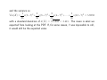
For example, if we generate 5 random numbers
.8147,
.9058 .1770 .9134 .6324
and we want integers ≤ 10 then x=floor (11*x ) ) gives {8, 9, 1, 10, 6}
and x=ceil ( 10*x ) gives {9, 10, 2, 10, 7}.
• The only thing that may be disconcerting is that if we run our program
which is based on generating random numbers two times in a row, we will
get different numbers! It is sometimes useful (such as in debugging) to be
able to reproduce your results exactly. If you continually generate random
numbers during the same Matlab session, you will get a different sequence
each time, as you would expect.
• However, each time you start a session, the random number sequence begins
at the same place (0.9501) and continues in the same way. This is not true
to life, as every gambler knows.
• Clearly we don’t want to terminate our session every time we want to reproduce results so we need a way to “fix” this. To do this, we provide a seed for
our random number generator. Just like Matlab has a seed at the beginning
of a session we will give it a seed to start with at the beginning of our code.
Seeding rand
• The random number generator rand can be seeded with the statement
rand(state, n)
where n is any integer. By default, n is set to 0 when a Matlab session
starts.
• Note that this statement does not generate any random numbers; it only
initializes the generator.
• Sometimes people will use the system clock to make sure the seed is being
reset
rand(state, sum(100 ∗ clock))
• Try setting the seed for rand, generating a random number, then resetting
the seed and generate another random number; see that you get the same
random number two times in a row; e.g.,
rand(′state′, 12345)
rand(1)
Exercise Use two calls to Matlab’s rand command to generate two random row
vectors of length 4. Now repeat the exercise where you reset the seed before
each call to rand. You should get the same vector each time in this latter case.
Probability Density Function
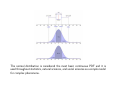
• If we measure a random variable many times then we can build up a distribution of the values it can take.
• As we take more and more measurements and plot them, we will see an
underlying structure or distribution of the values.
• This underlying structure is called the probability density function (PDF).
• For a discrete probability distribution the PDF associates a probability with
each value of a discrete random variable.
For example, let the random variable X be the number of rainy days in a
10 day period. The number of outcomes is 11 because we can have 0 days,
1 day, . . ., 10 days. The discrete PDF would be a plot of each probability.
• For a continuous probability distribution the random variables can take all
values in a given range so we can not assign probabilities to individual values.
Instead we have a continuous curve, called our continuous PDF, which allows
us to calculate the probability of a value within any interval.
• How will we determine the probability for a range of values from the continuous PDF? We will see that the probability is calculated as the area under
the curve between the values of interest.
• We first look at discrete PDFs.
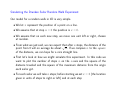
Estimating the Probabilities & the Discrete PDF
• If we have an experiment (like rolling dice or flipping a coin) we may be
able to compute the exact probabilities for each outcome (as we did in the
Fermat-Pascal problem) and then plot the PDF.
• But what if we don’t have the exact probabilities? Can we estimate them
and then use the estimates to plot the PDF?
The answer is yes. We essentially take many measurements of the random
variable and accumulate the frequency that each outcome occurred. The
relative frequency of each outcome gives us an estimate of its probability.
For example, if a particular outcomes occurs 50% of the time, then its probability is 0.5.
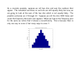
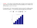
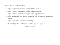
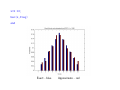
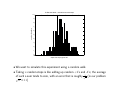
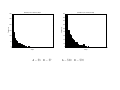
As a concrete example, suppose we roll two dice and sum the numbers that
appear. The individual outcomes on each die are still equally likely but now we
are going to look at the sum of the two dice which is not equally likely. The
possible outcomes are 2 through 12. Suppose we roll the dice 1000 times and
count the frequency that each sum appears. When we look at the frequency plot
for the sums we notice that it shows a nonuniformity. This is because there is
only one way to score 2, but many ways to score 7.
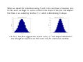
When we repeat the calculations using 3 and 4 dice and draw a frequency plot
for the sums, we begin to notice a trend in the shape of the plot and suspect
that there is an underlying function f (x) which is determining its shape.
• In fact, this plot suggests the normal curve, or ”bell shaped distribution”,
even though we expect to see that curve only for continuous variables.
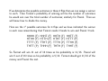
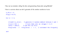
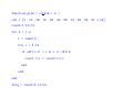
How can we simulate rolling the dice and generating these plots using Matlab?
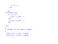
Here is a version where we don’t generate all the random numbers at once.
n_dice = 2;
freq(1:12)=0;
for k = 1:n
x=rand(1,n_dice);
% generate 2 random numbers between 0 and 1
x=ceil( 6*x );
% turn them into an integer 1 to 6
value = sum(x);
% sum the two dice
freq(value ) = freq(value ) + 1; % increment the frequency
end
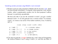
We can also generate all the random numbers for all the throws for the two dice
using
throws = rand(n, n dice);
throws = ceil(6 ∗ throws);
How can we use the frequency plot to estimate the probabilities?
• A frequency plot is simply a record of what happened.
• However, if we keep records long enough, we may see that the frequency
plot can be used to make statements about what is likely to happen in the
future. For two dice, we can say that a score of 7 is very likely and can even
guess how much more likely it is than say 3.
• This suggests that there is an underlying probability that influences which
outcomes occur. In cases where we are simply collecting data, we can turn
our frequencies into estimates of probability by normalizing by the total
number of cases we observed:
frequency of result #i
estimated probability of result #i =
total number of results
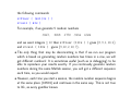
Now let’s compare the approximate probabilities found using this formula for the
case where we used n throws of 2 dice and then compare this with their exact
probabilities.
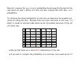
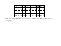
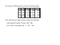
To calculate the actual probabilities of each sum we determine the possible outcomes of rolling the dice. Because there are more outcomes in this case, it’s
better to make an outcome table where we list all possible outcomes of the roll
of 2 (fair) dice.
1
2
3
4
5
6
1
(1,1)
(2,1)
(3,1)
(4,1)
(5,1)
(6,1)
2
(1,2)
(2,2)
(3,2)
(4,2)
(5,2)
(6,2)
3
(1,3)
(2,3)
(3,3)
(4,3)
(5,3)
(6,3)
4
(1,4)
(2,4)
(3,4)
(4,4)
(5,4)
(6,4)
5
(1,5)
(2,5)
(3,5)
(4,5)
(5,5)
(6,5)
6
(1,6)
(2,6)
(3,6)
(4,6)
(5,6)
(6,6)
• We see that there are a total of 36 combinations of the dice.
• If we want to compute the probability of an outcome, how would we do it?
As an example, consider the probability of the outcome (3,5). Remember
that these events are independent and because the probability of rolling a
3 with the first die is 1 out of 6 and the probability of rolling a 5 with
the second die is also 1 out of 6 so the probability of the outcome (3,5) is
1
1
1
×
=
.
6
6
36
• However, we want to determine the probability that a particular sum will
occur. The number of outcomes resulting in a sum of 2 to 12 are:
2→1
7→6
8→5
3→2
9→4
4→3
5→4
10 → 3
6→5
11 → 2
12 → 1
• How do we compute the probability that a particular sum will occur? Consider the probability of the sum 5 occurring. There are a total of 4 ways out
of 36 outcomes that yield the sum of 5 so its exact probability is 4/36=1/9.
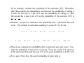
• For a pair of fair dice, the exact probability of each total is:
2
3
4
5
6
7
8
1
36
2
36
3
36
4
36
5
36
6
36
5
36
9 10 11 12
4
36
3
36
2
36
1
36
.03 .06 .08 .11 .14 .17 .14 .11 .08 .06 .03
Note that the probabilities are all positive and the sum of the probabilities is 1,
as expected.
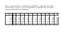
Now we compare these to our estimated probabilities. Clearly they don’t agree
but for large n they are a “good” approximation. Remember that are using a
frequency interpretation of probability.
sum →
2
3
4
5
6
7
8
9
10
11
12
exact .03
.06
.08
.11
.14
.17
.14
.11
.08
.06
.03
n = 100 .02
.05
.07
.09
.15
.12
.15
.11
.15
.07
.02
n = 1000 .034 .048 .082 .123 .136 .171 .127 .115 .091 .049 .024
n = 10000 .026 .0555 .0867 .1181 .1358 .1711 .1347 .1088 .0822 .0553 .0258
• Our plot of the exact probabilities is an example of a discrete PDF and the
corresponding plot of our estimated probabilities is an approximation to the
discrete PDF. The PDF assigns a probability p(x) to each outcome X in our
set Ω of all possible outcomes. In our example there were 11 outcomes and
Ω = {2, 3, 4, 5, 6, 7, 8, 9, 10, 11, 12} .
• Recall that the discrete PDF describes the relative likelihood for a random
variable to occur at a given point.
• What properties should a discrete PDF have? Clearly two obvious requirements for a discrete PDF are
1.
2.
0 ≤ p(xi) for each xi
Pn
i=1 p(xi) = 1 where n is the number of possible outcomes.
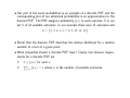
Exercise. Suppose you have a die which is not fair in the sense that each side
has the following probabilities
2
2
2
1
1
1
2→
3→
4→
5→
6→
1→
9
9
9
9
9
9
Would you bet on rolling an even or an odd number? Why?
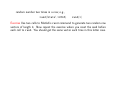
Write a code to simulate rolling one of these loaded dice and estimate the PDF.
Graph it.
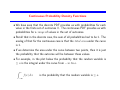
Continuous Probability Density Functions
• We have seen that the discrete PDF provides us with probabilities for each
value in the finite set of outcomes Ω. The continuous PDF provides us with
probabilities for a range of values in the set of outcomes.
• Recall that in the discrete case, the sum of all probabilities had to be 1. The
analog of that for the continuous case is that the total area under the curve
is 1.
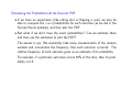
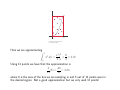
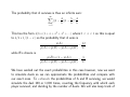
• If we determine the area under the curve between two points, then it is just
the probability that the outcome will be between those values.
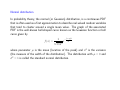
• For example, in the plot below the probability that the random variable is
≤ a is the integral under the curve from −∞ to a.
Z
a
f (x) dx
−∞
is the probability that the random variable is ≤ a.
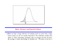
Mean, Variance and Expected Values
• When we have a large collection of numbers (such as scores from a large
lecture exam) we are not usually interested in the individual numbers but
rather in certain descriptive quantities such as average and how far from
the average a certain percentage of students are. The same is true for a
probability density function.
• Three important characteristics of a PDF are its mean or expected value or
average, its variance, and the standard deviation.
• For a discrete PDF, assume that we have a finite set Ω of all possible n
outcomes and the ith outcome for the random variable X is denoted by xi.
We can calculate the expected value (i.e., the mean) of a random variable
X, denoted either µ or E[X], from the formula
n
X
µ=
p(xi)xi
i=1
• For a continuous PDF, where the random variables range between a and b
we can calculate the mean from the formula
Z b
p(x)x dx
µ=
a
• If you recall the definition of the center of mass of a laminar sheet
R
DRxρ(x) dA
D ρ dA
whereR ρ is the density you can see an analog of this formula because in our
b
case a p dx = 1.
• To understand the discrete case, let’s look at an example.
Consider the situation where we have the heights in inches of the 12 members
of a women’s basketball team given by
{69, 69, 66, 68, 71, 65, 67, 66, 66, 67, 70, 72}
We know that if we want the average height of the players we simply compute
69 + 69 + 66 + 68 + 71 + 65 + 67 + 66 + 66 + 67 + 70 + 72
= 67.9
12
We can also interpret 67.9 as the mean or expected value of a random
variable. To see this, consider choosing one player at random and let the
random variable X be the player’s height. Then the expected value of X is
67.9 which can also be calculated by forming the product of each xi and its
corresponding probability
1
1
1
1
69
+ 69
+ 66
+ · · · + 72
12
12
12
12
which is just the formula we gave for the mean/expected value.
Example Suppose we are going to toss a (fair) coin 3 times. Let X, the random
variable, be the number of heads which appear. Find the mean or expected value
and explain what it means.
We know that there are 23 possible outcomes which are
HHH, HHT, HTH, HTT, TTT, TTH, THT, THH
and each has a probability of 1/8. Now heads can occur no times, 1 time, 2
times or 3 times. The probability that it occurs 0 times is 1/8, that it occurs 1
time is 3/8, that it occurs 2 times is 3/8 and it occurs 3 times is 1/8. Therefore
the mean or expected value is
3
3
1 12 3
1
= .
0 +1 +2 +3 =
8
8
8
8
8
2
This says that if we toss the coin three times the number of times we expect
heads to appear is 32 which is one-half the total possible times; exactly what we expected! Another way to get this answer is to consider the set {3, 2, 2, 1, 0, 1, 1, 2}
indicating the number of heads appearing in 3 tosses and average them to get
(3 + 2 + 2 + 1 + 0 + 1 + 1 + 2)/8 = 12/8 = 3/2.
Statisticians use the variance and standard deviation of a continuous random
variable X as a way of measuring its dispersion, or the degree to which it is
“scattered.”
The formula for the variance Var(X) of a discrete PDF is
Var(X) =
n
X
i=1
p(xi) ∗ (xi − µ))2
and for a continuous PDF
Var =
Z
b
a
p(x)(x − µ)2 dx
where µ is the expected value or mean.
p
The standard deviation, σ(X) is just Var(X).
Note that Var(X) is the mean or expected value of the function (X − µ)2, which
measures the square of the distance of X from its mean. It is for this reason that
Var(X) is sometimes called the mean square deviation, and σ(X) is called the
root mean square deviation. Var(X) will be larger if X tends to wander far
away from its mean, and smaller if the values of X tend to cluster near its mean.
The reason we take the square root in the definition of σ(X) is that Var(X)
is the mean/expected value of the square of the deviation from the mean, and
thus is measured in square units. Its square root therefore gives us a measure in
ordinary units.
Example Compute the mean (expected value), variance and standard deviation
for our example where we throw 2 dice and sum the values. Recall that here the
random variable X is the sum of the values.
Returning to our probability table
2 3 4 5 6 7 8 9 10 11 12
1 2 3 4 5 6 5 4
36 36 36 36 36 36 36 36
3
36
2
36
1
36
we can compute the mean or expected value as
µ=2
1
2
3
2
1
+ 3 + 4 + · · · + 11 + 12 = 7
36
36
36
36
36
and the variance as
2
3
1
1
2
2
2
Var(X) = ∗(2−7) + ∗(3−7) + ∗(4−7) +. . .+ ∗(12−7)2 = 5.8333
36
36
36
36
√
with a standard deviation of σ(X) = 5.833 = 2.415. The mean is what we
expected from looking at the PDF. If, for some reason, 7 was impossible to roll,
it would still be the expected value.
Normal distribution
In probability theory, the normal (or Gaussian) distribution, is a continuous PDF
that is often used as a first approximation to describe real-valued random variables
that tend to cluster around a single mean value. The graph of the associated
PDF is the well-known bell-shaped curve known as the Gaussian function or bell
curve given by
f (x) = √
1
2πσ 2
−
e
(x−µ)2
2σ 2
where parameter µ is the mean (location of the peak) and σ 2 is the variance
(the measure of the width of the distribution). The distribution with µ = 0 and
σ 2 = 1 is called the standard normal distribution.
The normal distribution is considered the most basic continuous PDF and it is
used throughout statistics, natural sciences, and social sciences as a simple model
for complex phenomena.
randn
Matlab has a built in command randn which returns pseudorandom values drawn
from the standard normal distribution. We can use it to generate values from a
normal distribution with a particular mean and standard deviation; for example,
if we want to generate 100 points with mean 1 and standard deviation 2 we use
r = 1 + 2. ∗ randn(100, 1);
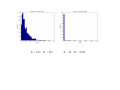
Example Generate 1000 random numbers using rand and randn and make
a histogram of the results. Compute the mean and standard deviation of each
using the Matlab commands mean and std. The command to make a histogram
of y values is hist(y).
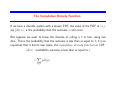
The Cumulative Density Function
If we have a discrete system with a known PDF, the value of the PDF at (xi),
say pdf(xi), is the probability that the outcome xi will occur.
But suppose we want to know the chances of rolling a 7 or less, using two
dice. This is the probability that the outcome is less than or equal to 7; it is so
important that it has its own name, the cumulative density function or CDF.
cdf(x) =probability outcome is less than or equal to x
=
X
y≤x
pdf(y)
Example If we return to the example when we rolled one die we know that
each number was equally probable so each had probability of 1/6. What is the
CDF for each xi ∈ {1, 2, 3, 4, 5, 6}?
If we ask what is cdf(6) then it should be 1 because we know it is 100% sure that
we will roll a number ≤ 6. For the other values we simply sum up the PDFs.
cdf(1) =
1
6
cdf(2) =
1 1 1
+ = ,
6 6 3
etc.
We see that for our discrete PDF
• cdf(x) is a piecewise constant function defined for all x;
• cdf(x) = 0 for x less than the smallest possible outcome;
• cdf(x) = 1 for x greater than or equal to the largest outcome;
• cdf(x) is essentially the discrete integral of pdf(X) over the appropriate
interval ;
• cdf(x) is monotonic (and hence invertible);
• the probability that x is between x1 and x2 ( x1 < x ≤ x2) is
.
cdf(x2) − cdf(x1)
Return again to the problem of rolling two dice and calculating the probability
that the sum of the dice is a number between 2 and 12. We found the exact
probability of each sum as:
2
3
4
5
6
7
8
1
36
2
36
3
36
4
36
5
36
6
36
5
36
9 10 11 12
4
36
3
36
2
36
1
36
.03 .06 .08 .11 .14 .17 .14 .11 .08 .06 .03
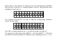
For a discrete case like this, it’s easy to make the corresponding cumulative
density function table:
2
3
4
5
6
7
8
1
36
3
36
6
36
10
36
15
36
21
36
26
36
9 10 11
30
36
33
36
35
36
12
36
36
.03 .08 .16 .28 .42 .58 .72 .83 .92 .97 1.00
The CDF is actually defined for all x, not just the values 2 through 12.
For example, the table tells us that cdf(4.3) = 0.16 and cdf(15) = 1 The latter
just tells us that the probability of rolling two dice and getting a sum ≤ 15 is 1.
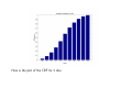
Here is the plot of the CDF for 2 dice.
Matlab has a built in command cumsum which can assist us in calculating the
CDF from a discrete PDF. For example, to find the cumulative sum of integers
from 1 to 5 we use
cumsum(1:5)
and the response is [ 1 3
6
10 15 ].
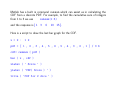
Here is a script to draw the last bar graph for the CDF.
x = 2 :
1 2
pdf = [ 1 , 2 , 3 , 4 , 5 , 6 , 5 , 4 , 3 , 2 , 1 ] / 3 6
cdf= cumsum ( pdf )
bar ( x , cdf )
xlabel ( ’ Score ’ )
ylabel ( ’CDF( Score ) ’ )
title ( ’CDF for 2 dice ’ )
Using the CDF for Simulation
• The CDF can be used to simulate the behavior of a discrete system.
• As an example, consider the problem of simulating rolling two dice and using
the CDF to estimate the probabilities where we are given the CDF as
cdf = {.03, .08, .16, .28, .42, .58, .72, .83, .92, .97, 1.00}
• First recall that the probability that x is between x1 and x2 is cdf(x2) −
cdf(x1).
• For our problem we generate a random number r between 0 and 1 for a
probability. We determine i such that
cdf(i − 1) < r ≤ cdf(i)
However, when i = 1 this doesn’t work so we append our CDF to include 0
cdf = {0, .03, .08, .16, .28, .42, .58, .72, .83, .92, .97, 1.00}
For example, if r = .61 then i = 8.
• We do this lots of times and keep track of how many random numbers were
assigned to i = 1, i = 2, etc.
• Then our estimate for the probability of the sum being say 2 (i.e., corresponding to i = 2) is the number of times we have chosen a random number
between 0 and 0.03 divided by the total number of random numbers generated.
function prob = cd sim ( n )
cdf = [0 .03 .08 .16 .28 .42 .58 .72 .83 .92 .97 1.00]
count(1:12)=0;
for k = 1:n
r = rand(1);
for i = 2:12
if cdf(i-1) < r & r <= cdf(i)
count (i) = count(i)+1;
end
end
end
freq = count(2:12)/n;
x=2:12;
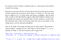
bar(x,freq)
end
Exact - blue
Approximate - red
Exercise. Let’s return again to the problem where we have a die which is not
fair in the sense that each side has the following probabilities
2
2
2
1
1
1
2→
3→
4→
5→
6→
1→
9
9
9
9
9
9
Compute the exact CDF. What is the probability that you will roll a 3 or less?
Write a program to use your CDF to approximate the exact probabilities. Compare.
The Monte Carlo Method
The Monte Carlo Method (MCM) uses random numbers to solve problems. Here
we will view MCM as a sampling method.
First we will see how we can sample different geometric shapes and then apply
the sampling to different problems.
The MC method is named after the city in the Monaco principality, because of
a roulette, a simple random number generator. The name and the systematic
development of Monte Carlo methods dates from about 1944.
The real use of Monte Carlo methods as a research tool stems from work on
the atomic bomb during the second world war. This work involved a direct
simulation of the probabilistic problems concerned with random neutron diffusion
in fissile material; but even at an early stage of these investigations, von Neumann
and Ulam refined this particular ” Russian roulette” and ”splitting” methods.
However, the systematic development of these ideas had to await the work of
Harris and Herman Kahn in 1948. Other early researchers into the field were
Fermi, Metropolis, and Ulam.
• We can think of the output of rand(), or any stream of uniform random
numbers, as a method of sampling the unit interval.
• We expect that if we plot the points along a line, they would be roughly
evenly distributed
• Random numbers are actually a very good way of exploring or sampling many
geometrical regions. Since we have a good source of random numbers for
the unit interval, it’s worth while to think about how we could modify such
numbers to sample these other regions.
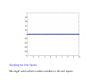
Sampling the interval [a, b]
Suppose we need uniform random numbers, but we want them in the interval
[a, b]
We have seen that we can use rand but now we have to shift and scale. The
numbers have to be shifted by a and scaled by b − a. Why?
r =rand();
s =a + (b − a) ∗ r
or we can do this for hundreds of values at once:
r =rand(10000, 1);
s =a + (b − a) ∗ r;
1000 uniformly sampled points on [1, 10]
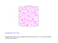
Sampling the Unit Square
We might need uniform random numbers in the unit square.
We could compute an x and y value separately for each point
x =rand();
y =rand();
or we can do this for hundreds of values at once to create a 2 × n array:
xy =rand(2, 10000);
Of course if our domain is not the unit square, then we must map the points.
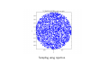
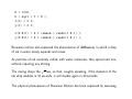
Sampling the Unit Circle
Suppose we need to evenly sample points in the unit circle; i.e., the circle centered
at (0,0) with radius 1.
The first thing that might come to mind is to try to choose a radius from 0 to
1, and then choose an angle between 0 and 2π
r =rand();
t =2 ∗ π ∗ rand();
but although this seems “random” it is not a uniform way to sample the circle
as the following figure demonstrates. More points in a circle have a big radius
than a small one, so choosing the radius uniformly actually is the wrong thing to
do!
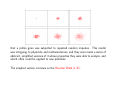
How can we fix this problem?
The problem is that when we choose the radius to vary uniformly, we’re saying
there are the same number of points at every value of the radius we choose
between 0 and 1. But of course, there aren’t. If we double the radius of a circle,
the area of the circle increases by a factor of 4. So to measure area uniformly, we
need r2 to be uniformly random, in other words, we want to set r to the square
root of a uniform random number.
p
r = rand();
t =2 ∗ π ∗ rand();
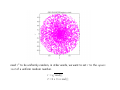
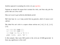
Another approach to sampling the circle is to use rejection.
Suppose we sample the square that contains the circle, and then only plot the
points that are in the circle?
Now we’re sure to get uniformly distributed points!
We’ll also have to reject many points that we generate, which of course is not
optimal.
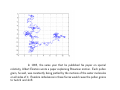
We imbed the unit circle in a square whose vertices are (-1,1), (1,-1), (-1,1),
(1,1).
x = -1 + 2 * rand ( );
y = -1 + 2 * rand ( );
i = find ( x.^2 + y.^2 < 1 )
plot ( x(i), y(i), ’b*’ )
In this example, there were 3110 points in the circle out of 4000 generated. Is
there any significance in this ratio?
Sampling using rejection.
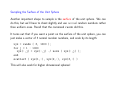
Sampling the Surface of the Unit Sphere
Another important shape to sample is the surface of the unit sphere. We can
do this, but we’ll have to cheat slightly and use normal random numbers rather
than uniform ones. Recall that the command randn did this.
It turns out that if you want a point on the surface of the unit sphere, you can
just make a vector of 3 normal random numbers, and scale by its length:
xyz = randn ( 3, 1000 );
for j = 1 : 1000
xyz(:,j) = xyz(:,j) ./ norm ( xyz(:,j) );
end
scatter3 ( xyz(1,:), xyz(2,:), xyz(3,:) )
This will also work for higher dimensional spheres!
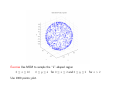
Exercise Use MCM to sample the “L”-shaped region
0 ≤ x ≤ 10
0 ≤ y ≤ 4 for 0 ≤ x ≤ 2 and 0 ≤ y ≤ 2 for x > 2
Use 1000 points; plot.
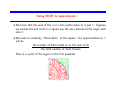
Using MCM to approximate π
• We know that the area of the unit circle (with radius 1) is just π. Suppose
we enclose the unit circle in a square say the one centered at the origin with
side 2.
• We want to randomly “throw darts” at the square. Our approximation to π
will be
the number of darts inside or on the unit circle
the total number of darts thrown
Here is a a plot of the region in the first quadrant.
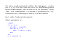
This method is easily implemented in Matlab. We simply generate a random
point (x, y) and decide if it is inside the circle or not. Because rand generates
random numbers between 0 and 1 we either have to map the numbers between
-1 and 1 or use numbers between 0 1 to calculate an approximation to π/4 (i.e.,
in the first quadrant) and multiply the result by 4; we choose the later.
Input: number of random points to generate
Output: approximation to π
count=0;
for i = 1, n
x=rand(1); y=rand(1);
if x^2+y^2 <= 1
count = count + 1 \par
end
end
pi = 4.*count / n
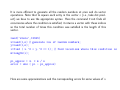
It is more efficient to generate all the random numbers at once and do vector
operations. Note that to square each entry in the vector x (i.e., take dot product) we have to use the appropriate syntax. Here the command find finds all
occurrences where the condition is satisfied; it returns a vector with these indices
so the total number of times this condition was satisfied is the length of this
vector.
rand(’state’,12345)
x=rand(1,n) % generate row of random numbers;
y=rand(1,n);
i=find ( x.^2 + y.^2 <= 1); % find locations where this condition is
m=length(i);
pi_approx = 4. * m / n
error = abs ( pi - pi_approx)
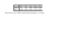
Here are some approximations and the corresponding errors for some values of n
101
102
103
104
105
Approx 3.2
3.16 3.164 3.1292 3.1491
Error 0.0584 0.0184 0.0224 0.0124 0.0075
Note that the error is NOT monotonically decreasing as n increases.
Buffon’s Needle Problem
An interesting related problem is Buffon’s Needle problem which was first proposed in 1777.
Here’s the problem (in a simplified form).
• Suppose you have a table top which you have drawn horizontal lines every 1
inch.
• You now drop a needle of length 1 inch onto the table.
• What is the probability that the needle will be lying across (or touching) one
of the lines?
2
• Actually, one can show that the probability is just
π
AA
A
A
A
X
XXX
XX
!
!!
!
!
So if we could simulate this on a computer, then we could have another method
for approximating π
• Let’s analyze the problem to see how we can implement it.
• Let’s assume without loss of generality that the lines are horizontal, they are
spaced 1 unit apart and the length of the needle is 1 unit.
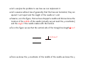
• Assume, as in the figure, that we have dropped a needle and that we know the
location of the middle of the needle (actually we just need the y-coordinate)
and the angle θ the needle makes with the horizon.
• So in the figure we see that the vertical side of the triangle has length 12 sin θ
θ
1/2 sin θ
• Since we know the y-coordinate of the middle of the needle we know the y
coordinates of the end of the needle
1
y ± sin θ
2
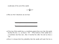
• Here are the 3 situations we can have
1
0
• If the top of the needle has a y-coordinate greater than one, then the needle
touches the line, i.e., we have a “hit”. If the bottom of the needle has a
y-coordinate less than zero, then it touches the other line and we have a
“hit”.
• Since it is known that the probability that the needle will touch the line is
2/π then
number of hits
2
≈
number of points π
and thus
number of points
π ≈2×
number of hits
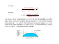
One way to see that the probability is 2/π is to note that the shaded portion in the
figure below is found by using the definite integral of (1/2)sin(theta) evaluated
from zero to pi. The result is that the shaded portion has a value of 1. The
value of the entire rectangle is (1/2)(pi) or pi/2. So, the probability of a hit is
1/(pi/2) or 2/pi. That’s approximately .6366197.
Exercise Write pseudo code for an algorithm to approximate π using Buffon’s
needle problem. Then modify the code for estimating π using the unit circle to
solve this problem.
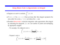
Using Monte Carlo to Approximate an Integral
• Suppose we want to evaluate
Z
b
f (x) dx
a
• If f (x) ≥ 0 for a ≤ x ≤ b then we know that this integral represents the
area under the curve y = f (x) and above the x−axis.
• Standard deterministic numerical integration rules approximate this integral
by evaluating the integrand f (x) at a set number of points and multiplying
by appropriate weights.
– For example, the midpoint rule is
Z b
a+b
(b − a)
f (x) dx ≈ f
2
a
– Simpson’s rule is
Z b
h
i
a+b
b−a
f (a) + 4f
+ f (b)
f (x) dx ≈
6
2
a
• Deterministic numerical integration (or numerical quadrature) formulas have
the general form
Z b
q
X
f (x) dx ≈
f (xi)wi
a
i=1
where the points xi are called quadrature points and the values wi are quadrature weights
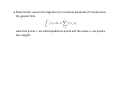
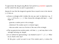
To approximate the integral using Monte Carlo (which is a probablistic approach)
we first extend the idea we used to approximate π.
Assume for now that the integrand is greater than or equal to zero in the interval
[a, b] then we
• choose a rectangle which includes the area you want to determine; e.g., if
f (x) ≤ M for all a ≤ x ≤ b then choose the rectangle with base b − a and
height M
– generate a random point in the rectangle
– determine if the random point is in desired region
– take area under curve as a fraction of the area of the rectangle
• First we generate two random points, call them (x, y) and map them to the
rectangle enclosing our integral.
• In our method for approximating π we checked to see if x2 + y 2 ≤ 1. What
do we check in this case?
At this given x-point we want to see if the random point y is above the
curve or not. It is easy to check to see if
y ≤ f (x) where x is the random point
If this is true, then the point lies in the desired area and our counter is
incremented.
• Our approximation to the area, i.e., the value of the integral, is simply
the usual fraction times the area of the testing rectangle (whose area is
M (b − a)).
number of hits
× M (b − a)
number of points
(2,4)
(2,0)
12 random points generated and
5 in the desired region
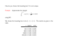
Here we are approximating
Z
2
3 2
x
8
2
x dx = = = 2.67
3 0 3
0
Using 12 points we have that the approximation is
40
5
(8) =
= 3.33
12
12
where 8 is the area of the box we are sampling in and 5 out of 12 points were in
the desired region. Not a good approximation but we only used 12 points!
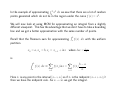
How do you choose the bounding box? It is not unique.
Example
Approximate the integral
Z 1/2
1
cos(πx) = ≈ 0.3183
π
0
using MC.
We choose the bounding box to be [0, .5] × [0, 1]. The results are given in the
table.
n approx
100
1000
10000
100,000
0.3150
0.3065
0.3160
0.3196
error
0.0033
0.0118
0.0023
0.0013
R2
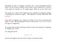
In the example of approximating 0 x2 dx we saw that there are a lot of random
points generated which do not lie in the region under the curve f (x) = x2.
We will now look at using MCM for approximating an integral from a slightly
different viewpoint. This has the advantage that we don’t have to take a bounding
box and we get a better approximation with the same number of points.
Recall that the Riemann sum for approximating
partition
Rb
a
f (x) dx with the uniform
x0 = a, xn = b, xi = xi−1 + ∆x where ∆x =
b−a
n
is
Z
b
a
f (x) dx ≈
n
X
i=1
f (x̃i)∆x =
n
X
i=1
b−a
f (x̃i)
n
Here x̃i is any point in the interval [xi−1, xi] so if x̃i is the midpoint (xi−1 + xi)/2
then we have the midpoint rule. As n → ∞ we get the integral.
The MCM approach to this problem can be written as
Z b
n
X
b−a
f (x) dx ≈
f (xi)
n
a
i=1
where now the points xi are random points in the interval [a, b]. This is not
a determinate formula because we choose the xi randomly. For large n, we can
get a very good approximation.
Another way to look at this expression is to recall from calculus that the average
of the function f (x) over [a,b] is
Z b
Z b
n
X
1
1
f (x) dx = (b − a)f¯ ≈ (b − a) ∗
f (x) dx =⇒
f (xi)
f¯ =
b−a a
n i=1
a
One can show rigorously that the error is O( √1n ).
Example
Consider the example we did before of approximating the integral
Z 1/2
1
cos(πx) = ≈ 0.3183
π
0
using MC. We now compare the two methods. We have to do the same number
of function values in each case.
n approx
error
100 0.3150 0.0033 0.3278 0.0095
1000 0.3065 0.0118 0.3157 0.0026
10000 0.3160 0.0023 0.3193 0.0010
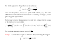
Example
where
Consider the problem of estimating a “hard” integral
R1
0
f (x) dx
f (x) =sech2(10.0 ∗ (x − 0.2))
+sech2(100.0 ∗ (x − 0.4))
+sech2(1000.0 ∗ (x − 0.6))
From the plot, it should be clear that this is actually a difficult function to
integrate. If we apply the Monte Carlo Method, we get “decent” convergence to
the exact value of 0.21080273631018169851
1
10
100
1000
10,000
100,000
1,000,000
0.096400
0.179749
0.278890
0.221436
0.210584
0.212075
0.211172
1.1e-01
3.1e-02
6.8e-02
1.0e-02
2.1e-04
1.2e-03
3.6e-04
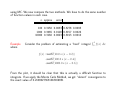
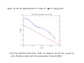
Here is a plot of the error on a log-log plot. Note that the slope is approximately
-1/2. This is what we expect because we said that the error = C √1n for a constant
C so the log of the error is log(n−1/2) = −0.5 log n.
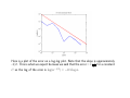
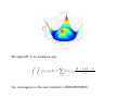
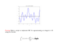
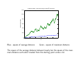
Now let’s approximate the integral of a function when the interval is not [0, 1].
Specifically we want to integrate
f (x) = cos(x)
+5∗ cos(1.6 ∗ x)
−2∗ cos(2.0 ∗ x)
+5∗ cos(4.5 ∗ x)
+7∗ cos(9.0 ∗ x);
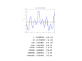
over [2,7]. This is a very“wiggly” function which we you can see from the plot.
Because the interval is [2, 7] we have to shift the interval from [0,1] to [2,7]. This
is easy to do with a linear map; we want 0 → 2 and 1 → 7 so the linear function
that does this is y = 2 + 5x so a random point x in the interval [2, 7] is just x
= 2.0 + ( 7.0 - 2.0 ) * rand ( n, 1 ).
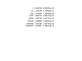
Applying the Monte Carlo Method, we get “decent” convergence to the exact
solution -4.527569. . .:
1
10
100
1000
10000
100000
1000000
10000000
21.486936
-21.701206
-2.472846
-4.911594
-4.253230
-4.424016
-4.509781
-4.529185
2.6e+01
1.7e+01
2.0e+00
3.8e-01
2.7e-01
1.0e-01
1.7e-02
1.6e-03
Again, we see the approximation to a slope of − 21 on a log-log plot.
• The two functions both seem “hard” to integrate, but for one, we got an
error 20 times smaller with the same number of points Why?
• The error depends in part on the variance of the function.
• To get a feeling for the variance of these
R btwo functions;2 remember that the
variance is given by the formula Var = a x(x − mean) dx.
– The first function has an integral of about 0.2 over the interval [0,1], so its
average value is 0.2 because the length of the interval is 1. The function
ranges between 0 and 1, so the pointwise variance is never more than
(1 − .2)2 = 0.64
– The second function has an integral of about -4.5 over an interval of
length 5, for an average value of about -1. Its values vary from -14 to
+16 or so, so the pointwise variance can be as much as 200.
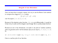
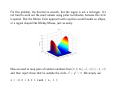
Integrals in two dimensions
Since we know how to sample a square, let’s try to use the Monte Carlo method
to compute the integral of f (x, y) where
f (x, y) = |x2 + y 2 − 0.75|
over the square [−1, +1] × [−1, +1].
Because of the absolute value function, f (x, y) is not differentiable. It would be
tricky to try to work out the integral, even though this is a pretty simple function.
Because we are in two dimensions, we need to use pairs of random numbers;
when we generate each it will be between [0,1] so we map to [−1, +1] × [−1, +1]
by
x= -1.0 + 2.0 * rand ( n, 1 ), y = -1.0 + 2.0 * rand ( n, 1 )
Here is a surface plot of our function.
We apply MC in an analogous way
Z dZ
c
a
b
f (x, y) dx ≈
n
X
i=1
f (xi, yi)
(b − a)(d − c)
n
Our convergence to the exact solution 1.433812586520645:
1
10
100
1000
10000
100000
1000000
10000000
0.443790
1.547768
1.419920
1.464754
1.430735
1.428808
1.432345
1.433867
9.900230e-01
1.139549e-01
1.389309e-02
3.094170e-02
3.077735e-03
5.004836e-03
1.467762e-03
5.394032e-05
Sometimes we have to integrate a function over a more complicated domain
where it is not as easy to sample in but we have a way to determine if a point is
in the region; for example, an “E”-shaped region. What can we do in that case?
The answer is to return to the original way we evaluated an integral by putting
a bounding box around the region. This approach is usually called MC with
rejection.
If we want to integrate over a region in 2-d that is not a box, we enclose that
region in a box. We then generate a point in the box and reject it if it is not in
the region of integration.
To see how this rejection technique works we look at the example of computing
an integral over a circle.
Our integrand will be
f (x, y) = x2
and we will integrate over the circle of radius 3 centered at (0,0).
For this problem, the function is smooth, but the region is not a rectangle. It’s
not hard to work out the exact answer using polar coordinates, because the circle
is special. But the Monte Carlo approach with rejection would handle an ellipse,
or a region shaped like Mickey Mouse, just as easily.
Now we need to map pairs of random numbers from [0, 1] to [−3, +3] × [−3, +3]
and then reject those that lie outside the circle x2 + y 2 = 9. We simply use
x = -3.0 + 6.0 * rand ( n, 1 );
y = -3.0 + 6.0 * rand ( n, 1 );
if x.^2 + y.^2 <= 9
Note that here we are generating n random numbers at once and using the vector
operation for exponentiation.
exact = 63.617251235193313079;
area = pi * 3*3;
% domain we are integrating over
x = - r + 2 * r * rand ( n, 1 );
y = - r + 2 * r * rand ( n, 1 );
i = find ( x .* x + y .* y <= r * r );
n2 = length ( i );
result = area * sum ( x(i) .* x(i) ) / n2;
fprintf ( 1, ’ %8d %f %e\n’, ...
n2, result, abs ( result - exact ) );
end
% because our funct
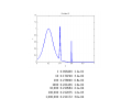
If we apply the Monte Carlo Method, we get “decent” convergence:
1
9
78
784
7816
78714
785403
7853972
74.493641
52.240562
62.942561
61.244910
62.653662
63.405031
63.669047
63.624209
1.087639e+01
1.137669e+01
6.746898e-01
2.372341e+00
9.635895e-01
2.122204e-01
5.179565e-02
6.958217e-03
Exact
63.617251235193313079
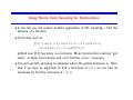
Using Monte Carlo Sampling for Optimization
• In the lab you will explore another application of MC sampling – find the
extrema of a function.
• A function such as
f (x) = cos(x) + 5 ∗ cos(1.6 ∗ x) − 2 ∗ cos(2.0 ∗ x)
+5∗ cos(4.5 ∗ x) + 7 ∗ cos(9.0 ∗ x);
plotted over [2,7] has many local extrema. Many minimization routines “get
stuck” at these local minima and can’t find the global minimum.
• You will use MC sampling to estimate where the global minimum is. Note
that if we have an algorithm to find a minimum of f (x), we can find its
maximum by find the minimum of −f (x).
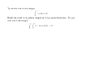
Exercise Write a script to implement MC for approximating an integral in 1D
using the formula
Z
b
a
f (x) dx ≈
n
X
i=1
f (xi)
b−a
n
Try out the code on the integral
Z
1
cos(4πx) dx
0
Modify the script to to perform integration in two spatial dimensions. Try your
code out on the integral
Z 3Z 2
(1 + 8xy) dydx = 57 .
0
1
Simulations using the Monte Carlo Method
• So far we’ve concentrated on the Monte Carlo method as a means of sampling. This gave us an alternate means of solving integration problems. Of
course, there are already other methods for dealing with integration problems.
• We will next consider a Monte Carlo application in which no other method
is available, the field of simulation.
• We will consider the common features of tossing a coin many times, watching
a drop of ink spread into water, determining game strategies, and observing
a drunk stagger back and forth along Main Street!
• Using ideas from the Monte Carlo method, we will be able to pose and
answer questions about these random processes.
• Computer simulation is intended to model a complex process. The underlying
model is made up of simplifications, arbitrary choices, and rough measurements.
• Our hope is that there is still enough relationship to the real world that we
can study the results of the simulation and get an idea of how the original
process works, predict outputs for given inputs, and how we can improve it
by changing some of the parameters.
• A famous applied mathematician once said “the purpose of computations is
insight, not numbers”. It is good to always keep this in mind!.
• Often it is particularly hard to use rigorous mathematical analysis to prove
that a given model will always behave in a certain way (for example, the
output won’t go to infinity.)
• Sampling tries to answer these questions by practical examples - we try lots
of inputs and see what happens.
• We want to consider some examples of simulations that can be done using
the MC method and you will look at another in the lab.
A Simple Example from Business
Suppose a friend is starting a business selling cookies and you want to help him
succeed (and show off your computational skills).
Assume he buys the cookies from a local bakery at the cost of $0.40 and sells
them for $1.00; assume that your friend has no overhead so he makes $0.60 in
profit per cookie if he sells all the ones he ordered.
However, if he has some cookies left over at the end of the day, those are given
to the homeless shelter and he looses $0.40 per cookie. He works for four hours
each afternoon and feels there is a fairly uniform demand during those hours; he
has never sold less than 80 or more than 140 cookies.
Use MC to recommend how many cookies he should order to maximize his profits.
How can we use MC to answer this question?
• Let Q denote the quantity that he orders; D the demand (amount sold)
• Set Q = 80
• Generate n replications of D; i.e., generate n random numbers between 80
and 140
• For each replication, compute the daily profit
• After n replications estimate the earnings ordering Q cookies by
P
daily profit
earnings =
n
• Repeat for integer values of Q between 80 and 140;
• Select the value of Q which yields the best earnings
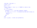
profit = 0.;
for k = 1:n
d = rand(1);
d=80 + 60*x;
if d > q
profit = profit + .6*q;
else
profit = profit + .6*d-.4*(q-d);
end
end
earnings = profit /n
end
60
58
56
54
52
50
48
80
90
100
110
120
130
140
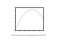
Profit is maximized by ordering approximately 116 cookies
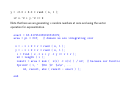
Brownian Motion
In 1827, Scottish botanist Robert Brown was studying pollen grains
which he had mixed in water. Although the water was absolutely
still, the pollen grains seemed to quiver and move about randomly.
He could not stop the motion, or explain it. He carefully described
his observations in a paper.
When other researchers were able to reproduce the same behavior, even using other liquids and other particles, the phenomenon was named
Brownian Motion, although no one had a good explanation for what they were
observing.
Check out the You Tube video for Brownian Motion at
http : //www.youtube.com/watch?v = apUl baT Kc
Here is the result of a simulation of Brownian motion.
In 1905, the same year that he published his paper on special
relativity, Albert Einstein wrote a paper explaining Brownian motion. Each pollen
grain, he said, was constantly being jostled by the motions of the water molecules
on all sides of it. Random imbalances in these forces would cause the pollen grains
to twitch and shift.
Moreover, if we observed the particle to be at position (x, y) at time t = 0, then
its distance from that point at a later time t was a normal random variable with
√
mean 0 and variance t. In other words, its typical distance would grown as t.
Recall that the command randn used here generates numbers with a normal
distribution.
T = 10.0;
N = 1000;
h = sqrt ( T / N );
x(1) = 0.0;
y(1) = 0.0;
for i = 1 : N
x(i+1) = x(i) + h * randn ( );
y(i+1) = y(i) + h * randn ( );
end
We can write this program another way to get rid of the loop.
T = 10.0;
N = 1000;
h = sqrt ( T / N );
x(1) = 0.0;
y(1) = 0.0;
x(2:N+1) = h * cumsum ( randn(1:N,1) );
y(2:N+1) = h * cumsum ( randn(1:N,1) );
Brownian motion also explained the phenomenon of diffusion, in which a drop
of ink in water slowly expands and mixes.
As particles of ink randomly collide with water molecules, they spread and mix,
without requiring any stirring.
√
The mixing obeys the t law, so that, roughly speaking, if the diameter of the
ink drop doubles in 10 seconds, it will double again in 40 seconds.
The physical phenomenon of Brownian Motion has been explained by assuming
that a pollen grain was subjected to repeated random impulses. This model
was intriguing to physicists and mathematicians, and they soon made a series of
abstract, simplified versions of it whose properties they were able to analyze, and
which often could be applied to new problems.
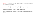
The simplest version is known as the Random Walk in 1D.
Random Walks
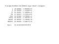
100 Drunken Sailors
We’ll introduce the random walk with a story about a captain whose ship was
carrying a load of rum. The ship was tied up at the dock, the captain was asleep,
and the 100 sailors of the crew broke into the rum, got drunk, and staggered out
onto the dock.
The dock was 100 yards long, and the ship was at the 50 yard mark. The sailors
were so drunk that each step they took was in a random direction, to the left
or right. (We’re ignoring the width of the pier because they can only move to
the right or left.) They were only able to manage one step a minute. Two hours
later, the captain woke up.
”Oh no!” he said, ”There’s only 50 steps to the left or right and they fall into
the sea! And two hours makes 120 steps! They will all be drowned for sure!”
But he was surprised to see that around 80 of the crew were actually within 11
steps to the left or right, and that all of the crew was alive and safe, though in
sorry shape.
How can this be explained?
We will use the idea of Random Walk to simulate it. Here’s a frequency plot for
the simulation.
1D Random Walk − 100 sailors and 120 steps
10
9
8
number of sailors
7
6
5
4
3
2
1
0
−40
−30
−20
−10
0
10
steps from ship right or left
20
30
40
• We want to simulate this experiment using a random walk.
• Taking n random steps is like adding up random +1’s and -1’s; the average
of such a sum tends to zero, with an error that is roughly √1n (in our problem
√
n ≈ 11)
1
√
|average − 0| ≈
n
then
|
and so
1
sum
|≈√
n
n
√
|sum| ≈ n.
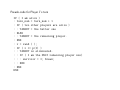
Simulating the Drunken Sailor Random Walk Experiment
Our model for a random walk in 1D is very simple.
• We let x represent the position of a point on a line.
• We assume that at step n = 0 the position is x = 0.
• We assume that on each new step, we move one unit left or right, chosen
at random.
• From what we just said, we can expect that
√ after n steps, the distance of the
point from 0 will on average be about n. If we compare n to the square
of the distance, we can hope for a nice straight line.
• First let’s look at how we might simulate this experiment. In this code we
want to plot the number of steps n on the x-axis and the square of the
distance traveled and the square of the maximum distance from the origin
each sailor got.
• For each sailor we will take n steps; before starting we set x = 0 (the location
given in units of steps to right or left) and at each step
– generate a random number r between 0 and 1(we could have mapped r
between -1 and 1)
– if 0 ≤ r < 0.5 we move to the left so x = x − 1
– if .5 < r ≤ 1 we move to the right so x = x + 1
%
%
Take WALK_NUM walks, each of length STEP_NUM random +1 or -1 step
time=1:step_num;
for walk = 1 : walk_num
x = 0;
for step = 1 : step_num
r = rand ( );
%
%
%
Take the step.
if ( r <= 0.5 )
x = x - 1;
else
x = x + 1;
end
%
%
Update the average and max.
x2_ave(step) = x2_ave(step) + x^2;
x2_max(step) = max ( x2_max(step), x^2 );
end
x2_ave(:,:) = x2_ave(:,:) / walk_num;
%
%
Plot the results.
plot ( time, x2_ave, time, x2_max, ’LineWidth’, 2 );
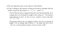
2
1D Random Walk − Max and average of distance versus time
1200
1000
Distance Squared
800
600
400
200
0
0
20
Blue - square of average distance
40
60
N
80
100
120
Green - square of maximum distance
The square of the average distance behaves linearly but the square of the maximum distance each sailor traveled from the starting point varies a lot.
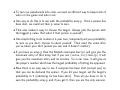
• In 1D, how many possible random walks of n steps are there?
• To answer this, consider flipping a coin. If we flip it once, there are two
choices H and T . If we flip it two times there are 22 = 4 choices
HH HT T T T H
and if we flip it 3 times there are 23 = 8 choices
HHH HHT HT H HT T T T T T HT T HH T T H
so in general there are 2n outcomes for flipping a coin n times.
• Our random walk in 1D is like flipping a coin; there are only two choices –
right or left.
• So if we have 120 steps 2120 ≈ 1036 possible random walks.
• How many of them can end up at a given position?
• There is only one that can end up at n.
• There are n out of 2n (i.e., 120 out of 1036) that end at n − 2; they involve
n − 1 steps of +1 and one step of -1; these can occur at n places. For
example, one sailor could go left on the first step and right on all remaining
ones; another sailor could go right on all steps except the second one, etc.
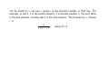
• One can show that, in general, there are
end up at n - 2*k.
n
k
distinct random walks that will
• That means the probability of ending up at a particular spot is just the
corresponding combinatorial coefficient divided by 2n.
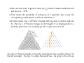
• In other words, row n of Pascal’s triangle tells you what a random walk can
do. But row n of Pascal’s triangle can be thought of as dropping balls in a
pachinko game that can randomly go left or right at each level!
An entry in Pascal’s triangle is found by summing the two numbers above it to
the left and right. The top 1 is called the zeroth row. An entry in the nth row
can be found by n choose r where r is the element number in that row. For
example, in row 3, 1 is the zeroth element, 3 is element number 1, the next three
is the 2nd element, and the last 1 is the 3rd element. The formula for n Choose
r is
n!
where 0!=1
r!(n − r)!
Random Walks in 2D
We can do the same thing in two dimensions. Now we can move to the right or
left or to the top or bottom. You will implement this in the lab and use a random
walk to solve Laplace’s equation in two dimensions.
Exercise Modify the code for using random walks for the drunken sailor problem
if each sailor has a 60% chance of moving to the right and a 40% chance of moving
to the left. Output your results in a frequency plot where the x axis is the number
of steps in each direction from the origin and the y axis is the frequency.
Game Theory
In the 1950’s, John von Neumann (who wrote the first computer user manual,
for the ENIAC), developed game theory, which sought strategies in multi-player
games. The Monte Carlo method was used to simulate the games, and determine
the best strategies. We will look at two examples of this – simulating a gambling
game and simulating a duel!
The first example is a modification to the Fermat/Pascal point game which makes
it much more difficult. Recall in that problem that if one person won, the other
person did not lose. Here we assume that one player wins a dollar from the other
player.
In particular, assume that there are two gamblers, A and B, who decide to play
a game.
A has p dollars and B has q dollars
They decide to flip a coin. If it comes up heads, A wins $1 from B while tails
works the other way.
The game is over when one gambler is bankrupt.
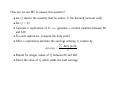
Here are some questions we can ask:
1. What is the probability that A will win?
2. What is the expected value of the game to A, that is, how much will he win
or lose, on average?
3. How long will a typical game last?
4. What are the chances that the winner will be ahead the entire game?
5. What happens if we change the amount of money that A and B have?
Here’s a typical game, in which A starts with $3 and B with $7; assume A wins
when a head comes up
0
A
B
3
7
1
H
4
6
2
H
5
5
3
T
4
6
4
T
3
7
5
T
2
8
6
H
3
7
7
T
2
8
8
T
1
9
9 10 11 12 13 14 15
H T H H T T T
2 1 2 3 2 1 0
8 9 8 7 8 9 10
A loses after 15 tosses, having tossed 6 heads and 9 tails.
Clearly the gambler with the most starting money has an advantage, but how
much?
It’s easy to see that if A starts with $3 dollars, the game can end in 3 steps. Can
we expect that in such a case, a typical game might last 6, or 9 or 12 steps?
Does it depend in any way on how much more money B has?
Suppose that A and B start with the same amount of money. In a typical game,
is it likely that they will each be in the lead about the same number of tosses?
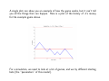
A single plot can show you an example of how the game works, but it can’t tell
you all the things that can happen. Here is a plot of the history of A’s money
for the example game above.
For a simulation, we need to look at a lot of games, and we try different starting
bets (the “parameters” of this model).
Let’s consider the following cases when we run our simulations:
$A $B
$3
$7
$30 $70
$10 $10
$1 $100
Remarks
Our starting example.
10 times as long?
Equal stakes, equal odds
Game will be quick.
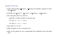
Structure of the code
• input starting stakes a stakes, b stakes and number of games to simulate n games
• initialize; set a wins=0, b wins=0, a=a stakes, b=b stakes
• for each game while a>0 and b>0
– generate a random number to see who wins
– if a wins, a = a+ 1; b=b-1
– if b wins, b = b+ 1; a=a-1
• stop when a=0 or b=0
• after the game is over, increment wins
• after all the games are over, approximate the probability that each player
wins
a_wins = 0;
b_wins = 0;
%
%
%
Play n_game games.
for game = 1 : n_games
a = a_stakes;
b = b_stakes;
while ( 0 < a & 0 < b )
r = rand ( );
if ( r <=
a = a +
b = b else
a = a -
0.5 )
1;
1;
1;
b = b + 1;
end
end
% increment wins
if ( b == 0 )
a_wins = a_wins + 1;
else
b_wins = b_wins + 1;
end
end
%
%
%
Average over the number of games.
prob_a_win = a_wins / n_games
prob_b_win = b_wins / n_games
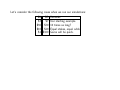
The results of 1000 games for each set of starting stakes.
$A $B Length Max A Prob
$3
$7
21
135
0.29
$30 $70 2,010 12,992
0.28
$10 $10
101
722
0.49
$1 $100
104 10,472
0.01
From this data you might be able to guess the following:
• the expected number of steps is $A * $B;
• A’s chance of winning is $A / ( $A + $B ) ;
What is the expected value of this game?
$A
A’s chance of winning is
$A + $B
the chance of $A losing (i.e., B winning) is 1 - this probability, or
$B
.
$A + $B
The expected value is
value(win) ∗ p(win) + value(loss) ∗ p(loss)
or
$B
$A
$B
− $A
=0
$A + $B
$A + $B
so even when A has $1 against B’s $100, it’s a fair game.
(small chance of big win) - ( big chance of small loss).
Here are the results of four simulations which mimic our cases above.
Gambler’s ruin, number of steps
Gambler’s ruin, number of steps
300
180
160
250
140
120
Frequency
Frequency
200
150
100
100
80
60
40
50
20
0
0
50
100
150
200
250
0
0
2000
4000
6000
Steps
A − $3 B − $7
8000
Steps
A − $30 B − $70
10000
12000
14000
A − $10 B − $10
A − $1 B − $100
Game Theory - Simulating a Duel
Another example in game theory is a duel. Two players take turns firing at each
other until one is hit. The accuracy, or probability of hitting the opponent on
one shot, is known for both players.
In the two person duel there is no strategy (just keep firing), but we want to
know the probabilities that either player survives.
If we assume Player A has an accuracy of 46 and Player B an accuracy of
A gets the first shot then Player A can survive if:
1. A hits on the first shot: ( probability: 4/6) OR
2. A misses, B misses, A hits ( probability: 2/6)*(1/6)*(4/6) OR
3. A misses, B misses, A misses, B misses, A hits:
( probability: 2/6)*(1/6)*(2/6)*(1/6)*(4/6)
OR...
5
6
and
The probability that A survives is thus an infinite sum:
∞
X
5 4
4
((1 − )(1 − ))i
6
6 6
i=0
This has the form 4/6 ∗ (1 + x + x2 + x3 + ...) where 0 < x < 1 so this is equal
to 4/6 ∗ 1/(1 − x) so the probability that A wins is
while B’s chance is
12
p(A)
=
p(A) + p(B) − p(A) ∗ p(B) 17
p(B) ∗ (1 − p(A))
5
=
p(A) + p(B) − p(A) ∗ p(B) 17
We have worked out the exact probabilities in this case however, now we want
to simulate duels so we can approximate the probabilities and compare with
our exact ones. To estimate the probabilities of A and B surviving, we would
simulate the duel 100 or 1,000 times, counting the frequency with which each
player survived, and dividing by the number of duels. We will also keep track of
the number of turns it takes to complete a duel (i.e., until we get a hit) and then
compute the average.
Basically we just need a function which performs the duel and returns the number
of shots required and the survivor (either Player 1 or Player 2). The only input
that is needed is p(1:2) which stores each player’s probability. We can then
write a script to call this function n duel times (the number of duels we are
simulating) and compute the average number of shots required to end the duel.
We would also keep a tally of how many duels were won by each player in the
calling script so we can estimate probabilities.
How do we decide if the player shooting hits the other player? We generate a
random number r between 0 and 1; then Player 1 hits his target if r ≤ p(1);
similarly for Player 2. The duel continues until a target is hit.
[survivor, turn_num] = function duel (p)
turn_num = 0; % count for number of shots required to complete due
if p(1) <= 0
& p(2) <=0
% make sure input probabilities are valid
fprintf (’invalid probabilities so duel fails’, /n)
return
end
while ( 1 )
%
%
%
Player 1 fires.
turn_num = turn_num + 1;
r = rand ( );
if ( r <= p(1) ) % Player 1 hits his target
survivor = 1;
break % leave the while loop
end
%
%
%
Player 2 fires.
turn_num = turn_num + 1;
r = rand ( );
if ( r <= p(2) ) % Player 2 hits his target
survivor = 2;
break
end
end
Note the use of the while (1) here. The expression which must be satisfied in
this statement is always true so the only way to escape the loop is through the
break statement. This is why we added a check at the first of the program to
verify that not both probabilities are ≤ 0.
A 3 person duel is more interesting and we will look at it next.
Exercise Download the function duel.m which has the code described above
implemented. Then write a script which calls this function for each simulation
of a duel. The input for your script should be the probabilities of each player
p(1:2) and the number of simulations you wish to perform. Your code should
(i) compute the average number of shots to complete the duel and (ii) estimate
the probabilities and compare with exact. After this is done, make a plot of the
average number of shots required versus the exact probability of Player 1.
The Three-Way Duel from ”The Good, The Bad, and The Ugly”
In a two person duel there’s no strategy (except of course to shoot at your
opponent on your turn).
But suppose we move to a three person duel involving A, B, and C. Let’s suppose
that C is a relatively poor shot.
If A and B are ”reasonable”, they will probably shoot at each other, since each
represents the biggest threat to the other. As soon as one gets hit, it will be C’s
turn, and that’s his best chance, to have the first shot at the remaining opponent.
(Remember they take turns shooting.)
But a disaster occurs if, instead of A or B knocking the other out, poor shot C
accidentally hits A or B on his turn. Because then C does not get the next shot;
rather the survivor gets first shot at C, and we know that whether A or B shoots
either is a better shot than C!
Now the coding for this problem is similar to that for the two person duel, except
that, on each shot, the player has a choice of whom to shoot at. We said A and
B should shoot at each other.
It seems that C should shoot at the better shot, say A, so that if he accidentally
hits him, he has to face the weaker player B.
Another possibility: C could shoot at no one (if that’s allowed). Then, once A
or B is out, C is sure to get the first shot at the survivor.
Coding the Three Person Duel
• The three-way duel is harder. Instead of writing it from scratch let’s see
what we need to change in the two-way duel code. When we do this, we
should see what we would have to revise if we had a four-person duel!
• Now we can’t assume that as soon as one person is eliminated, the game is
over. So the first thing we have to change is the part of the code that says
if the shot is accurate, the game is over and the shooter is the winner.
• Another issue is that now we have a choice of who to aim at. We will take
the rational strategy that each player aims at the other player who is the
most accurate shot.
• A “brute force” approach to coding this would be to write out what Player
1 will do, then what Player 2 will do and so on. This is straightforward, but
cluttered. It might be better to try to abstract what is going on.
• To this end, let’s concentrate on one arbitrary player whose index is I (i.e.,
1, 2, or 3). If it is I’s turn then what should he do?
– check to see if he is alive; if alive proceed;
– decide who to aim at (there may be one or two choices) based on their
probabilities;
– generate a random number and see if he hits his target;
– if he hits his target then check to see if he is the only surviving ;
– if he is the only survivor then set I as the survivor and return.
Pseudo-code for Player I’s turn
IF ( I am alive )
: turn_num = turn_num + 1
: IF ( two other players are alive )
: : TARGET = the better one
: ELSE
: : TARGET = the remaining player.
: END
: r = rand ( );
: IF ( r <= p(I) )
: : TARGET is eliminated.
: : IF ( I am the ONLY remaining player now)
: : : survivor = I; break;
: : END
: END
END
• To turn our pseudocode into code, we need an efficient way to keep track of
who’s in the game and who’s out.
• One way to do this is to use with the probability array p. Once a person has
been shot, we could set their p value to zero.
• That also makes it easy to choose the target. Always pick the person with
the biggest p value. But what if that person is yourself!
• One simple thing to do is when it is your turn, temporarily set your probability
to zero so you don’t choose to shoot yourself. Then reset the value after
you’ve taken your shot (unless you win and it doesn’t matter).
• If you have an array p then the Matlab command max(p) will give you the
maximum entry of that array; but if you use [value,loc]=max(p) it will
give you the maximum entry and its location. So in our case, it will give us
the player’s number which has the largest probability of hitting his opponent.
• Now there is an easy way to see if everyone has been shot (except you) so
that you can be declared the winner. If you hit your target, set the target’s
probability to 0 (indicating he has been shot). Then all you have to do is
sum the probability array p and if you get 0, then you are the only survivor.
Remember that you have temporarily set your probability to 0 so you won’t
shoot yourself.
turn_num = turn_num + 1;
p_save = p(i);
p(i) = 0.0;
[ pmax, target ] = max ( p ); % TARGET is index of max.
r = rand ( );
if ( r <= p_save )
p(target) = 0.0; % you shot opponent "target"
if ( sum ( p ) == 0.0 ) % everyone has been shot except you
survivor = i;
break;
end
end
p(i) = p_save; % reset your probability
Conclusion for Three-Way Duel
• This is not the best way, or the only way, but it is a way, and it has some
real advantages.
• There are hardly any extra variables (except for p save).
• The code works the same for every player. We never assume that the players
were given in a particular order.
• The code works the same if we increase the number of players.
• Your homework will be simulate a three-person duel using this strategy and
then to modify your code to change the strategy.