Download 5.5 Example: skew plate Example: skew plate Example

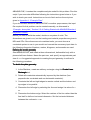
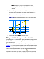
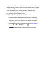
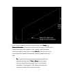
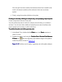
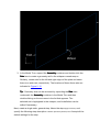
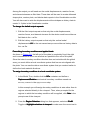
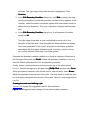
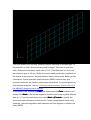
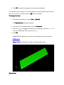
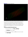
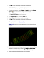
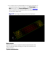
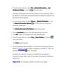
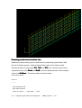
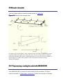
5.5 Example: skew plate
You have been asked to model the plate shown in Figure 5–9.
Figure 5–
5–9 Sketch of the skewed plate.
It is skewed 30° to the global 1-axis, is built-in at one end, and is constrained to move
on rails parallel to the plate axis at the other end. You are to determine the midspan
deflection when the plate carries a uniform pressure. You are also to assess whether a
linear analysis is valid for this problem. You will perform an analysis using
ABAQUS/Standard.
5.5.1 Preprocessing—
Preprocessing—creating the model with ABAQUS/CAE
Use ABAQUS/CAE to create the entire model for this simulation. A Python
script is provided in “Skew plate,” Section A.3. When this script is run through
ABAQUS/CAE, it creates the complete analysis model for this problem. Run this
script if you encounter difficulties following the instructions given below or if you
wish to check your work. Instructions on how to fetch and run the script are
given in Appendix A, “Example Files.”
If you do not have access to ABAQUS/CAE or another preprocessor, the input
file required for this problem can be created manually, as discussed in
“Example: skew plate,” Section 5.5 of Getting Started with ABAQUS/Standard:
Keywords Version.
Before you start to build the model, decide on a system of units. The
dimensions are given in cm, but the loading and material properties are given in
MPa and GPa. Since these are not consistent units, you must choose a
consistent system to use in your model and convert the necessary input data. In
the following discussion Newtons, meters, kilograms, and seconds are used.
Defining the model geometry
Start ABAQUS/CAE, and create a three-dimensional, deformable body with a
planar shell base feature. Name the part Plate, and specify an approximate part
size of 4.0. A suggested approach to creating the part geometry is outlined in
the following procedure:
To sketch the plate
plate geometry:
1. In the Sketcher, create an arbitrary rectangle using the Create Lines:
Rectangle tool.
2. Delete all constraints automatically imposed by the sketcher (four
perpendicular constraints and one horizontal constraint).
3. Constrain the left and right edges to remain vertical and the bottom and
top edges to be parallel.
4. Dimension the left edge by selecting the line and assign it a value of 0.4
m.
5. Dimension the bottom edge. Select the vertices of the line rather than the
line itself to define a horizontal dimension. Set the horizontal distance
between the vertices to 1.0 m.
Note: If you were to dimension the line itself, you would
control only the length of the line (in whatever orientation it
assumes).
6. Dimension the angle between the left and bottom edges. Select the left
and bottom edges in succession, and set the value of the angle to 60°.
The final sketch is shown in Figure 5–10.
Figure 5–
5–10 Sketch of the plate geometry (1 out of 2 grid lines visible).
7. In the prompt area, click Done to finish the sketch.
Defining the material and section properties
properties and the local material directions
The plate is made of an isotropic, linear elastic material with a Young's modulus
E = 30 × 109 Pa and a Poisson's ratio = 0.3. Create the material definition;
name the material Metal.
The orientation of the structure in the global coordinate system is shown in
Figure 5–9. The global Cartesian coordinate system defines the default material
directions, but the plate is skewed relative to this system. It will not be easy to
interpret the results of the simulation if you use the default material directions
because the direct stress in the material 1-direction,
, will contain
contributions from both the axial stress, produced by the bending of the plate,
and the stress transverse to the axis of the plate. It will be easier to interpret the
results if the material directions are aligned with the axis of the plate and the
transverse direction. Therefore, a local rectangular coordinate system is needed
in which the local
-direction lies along the axis of the plate (i.e., at 30° to the
global 1-axis) and the local
-direction is also in the plane of the plate.
Following the instructions given below, define the shell section properties in a
local (nondefault) material coordinate system.
To define shell section properties
properties and local material directions:
1. Define a homogeneous shell section named PlateSection. Specify that
section integration be performed before the analysis since the material is
linear elastic. Assign a shell thickness of 0.8E-2 and the Metal material
definition to the section.
2. Define a rectangular datum coordinate system as shown in Figure 5–11
using the Create Datum CSYS: 2 Lines tool
.
Figure 5–
5–11 Datum coordinate system used to define local material
directions.
3. From the main menu bar of the Property module, select Assign
Material Orientation and select the entire part as the region to which local
material directions will be applied. In the viewport, select the datum
coordinate system created earlier. Select Axis–
Axis–3 for the direction of the
approximate shell normal. No additional rotation is needed about this
axis.
Tip: To verify that the local material directions have been
assigned correctly, select Tools
Query from the main
menu bar and perform a property query on the material
orientations. Triads appear in the viewport indicating the
material orientation of the region you select.
Once the part has been meshed and elements have been created in the
model, all element variables will be defined in this local coordinate
system.
4. Finally, assign the section definition to the plate.
Creating an assembly, defining an analysis step, and specifying output requests
Create a dependent instance of the plate.
You will partition the plate in half at its midspan; this will allow you to define a
set there. You will also define additional assembly-level sets to facilitate other
output request and boundary condition definitions.
To partition the plate and define geometry sets:
1. In the Model Tree, double-click the Plate item in the Parts container to
make it current.
2. Partition the plate in half using the Partition Face: Shortest Path Between
2 Points tool,
. Use the midpoints of the skewed edges of the plate to
create the partition shown in Figure 5–12.
Figure 5–
5–12 Partition used to define a geometry set at the plate midspan.
3. In the Model Tree, expand the Assembly container and double-click the
Sets item to create a geometry set for the midspan named MidSpan.
Similarly, create sets for the left and right edges of the plate and name
them EndA and EndB, respectively. The locations of these three sets are
indicated in Figure 5–12.
Tip:
Tip: Geometry sets can be reviewed by expanding the Sets item
underneath the Assembly container in the Model Tree and then
double-clicking on the set name in the list that appears. The
selected set is highlighted in the viewport, and its definition can be
edited if necessary.
Next, create a single static, general step. Name the step Apply Pressure, and
specify the following step description: Uniform pressure (20 kPa) load. Accept all the
default settings for the step.
Among the output you will need are the nodal displacements, reaction forces,
and element stresses as field data. These data will be used to create deformed
shape plots, contour plots, and tabular data reports in the Visualization module.
You will also want to write the displacements at the midspan as history data to
create X–Y plots in the Visualization module.
To change the default output requests:
1. Edit the field output request so that only the nodal displacements,
reaction forces, and element stresses for the whole model are written as
field data to the .odb file.
2. Edit the history output request so that only the vertical nodal
displacements U3 for the set named MidSpan are written as history data to
the .odb file.
Prescribing boundary conditions and applied loads
As shown in Figure 5–9, the left end of the plate is completely fixed; the right
end is constrained to move on rails that are parallel to the axis of the plate.
Since the latter boundary condition direction does not coincide with the global
axes, you must define a local coordinate system that has an axis aligned with
the plate. You can use the datum coordinate system that you created earlier to
define the local material directions.
To assign boundary
boundary conditions in a local coordinate system:
1. In the Model Tree, double-click the BCs container and define a
Displacement/Rotation mechanical boundary condition named Rail
boundary condition
in the Apply Pressure step.
In this example you will assign boundary conditions to sets rather than to
regions selected directly in the viewport. Thus, when prompted for the
regions to which the boundary condition will be applied, click Sets in the
prompt area of the viewport.
2. From the Region Selection dialog box that appears, select set EndB.
EndB
Toggle on Highlight selections in viewport to make sure the correct set is
selected. The right edge of the plate should be highlighted. Click
Continue.
Continue
3. In the Edit Boundary Condition dialog box, click Edit to specify the local
coordinate system in which the boundary condition will be applied. In the
viewport, select the datum coordinate system that was created earlier to
define the local directions. The local 1-direction is aligned with the plate
axis.
4. In the Edit Boundary Condition dialog box, fix all degrees of freedom
except for U1.
U1
The right edge of the plate is now constrained to move only in the
direction of the plate axis. Once the plate has been meshed and nodes
have been generated in the model, all printed nodal output quantities
associated with this region (displacements, velocities, reaction forces,
etc.) will be defined in this local coordinate system.
Complete the boundary condition definition by fixing all degrees of freedom at
the left edge of the plate (set EndA).
EndA Name this boundary condition Fix left end.
Use the default global directions for this boundary condition.
Finally, define a uniform pressure load across the top of the shell named
Pressure.
Select both regions of the part using [Shift]+Click and then click Done
Done.
When prompted to choose a side for the shell or internal faces, select Brown,
Brown
which corresponds to the top side of the plate. You may need to rotate the view
to more clearly distinguish the top side of the plate. Specify a load magnitude of
2.E4
Pa.
Creating
Creating the mesh and defining a job
Figure 5–13 shows the suggested mesh for this simulation.
Figure 5–
5–13 Suggested mesh design for the skewed plate simulation.
You must answer the following questions before selecting an element type: Is
the plate thin or thick? Are the strains small or large? The plate is quite thin,
with a thickness-to-minimum span ratio of 0.02. (The thickness is 0.8 cm and
the minimum span is 40 cm.) While we cannot readily predict the magnitude of
the strains in the structure, we think that the strains will be small. Based on this
information, choose quadratic shell elements (S8R5) because they give
accurate results for thin shells in small-strain simulations. For further details on
shell element selection, refer to “Choosing a shell element,” Section 23.6.2 of
the ABAQUS Analysis User's Manual.
In the Model Tree, expand the Plate item underneath the Parts container and
double-click Mesh in the list that appears. Seed the part using a global element
size of 0.1. From the main menu bar, select Mesh
Controls to specify the
structured mesh technique for this model. Create a quadrilateral mesh using
quadratic, reduced-integration shell elements with five degrees of freedom per
node (S8R5).
Before proceeding, rename the model to Linear. This model will later form the
basis of the model used in the skew plate example discussed in Chapter 8,
“Nonlinearity.”
Define a job named SkewPlate with the following description:
Linear Elastic Skew Plate. 20 kPa Load.
Save your model in a model database file named SkewPlate.cae.
Submit the job for analysis, and monitor the solution progress; correct any
modeling errors detected by the analysis product, and investigate the cause of
any warnings.
5.5.2 Postprocessing
This section discusses postprocessing with ABAQUS/CAE. Both contour and
symbol plots are useful for visualizing shell analysis results. Since contour
plotting was discussed in detail in Chapter 4, “Using Continuum Elements,” we
use symbol plots here.
In the Module list located under the toolbar, click Visualization to enter the
Visualization module. Then, open the .odb file created by this job (SkewPlate.odb).
By default, ABAQUS/CAE plots the undeformed shape of the model.
Element normals
Use the undeformed shape plot to check the model definition. Check that the
element normals for the skew-plate model were defined correctly and point in
the positive 3-direction.
To display the element normals:
1. From the main menu bar, select Options
Common;
Common or use the
tool
in the toolbox.
The Common Plot Options dialog box appears.
2. Click the Normals tab.
3. Toggle on Show normals,
normals and accept the default setting of On elements.
elements
4. Click OK to apply the settings and to close the dialog box.
The default view is isometric. You can change the view using the options in the
view menu or the view tools (such as
) from the toolbar.
To change the view:
1. From the main menu bar, select View
Specify.
Specify
The Specify View dialog box appears.
2. From the list of available methods, select Viewpoint.
Viewpoint
3. Enter the
-,
- and
-coordinates of the viewpoint vector as –0.2, –1, 0.8
and the coordinates of the up vector as 0, 0, 1.
4. Click OK.
OK
ABAQUS/CAE displays your model in the specified view, as shown in
Figure 5–14.
Figure 5–
5–14 Shell element normals in skewed plate model.
Symbol plots
Symbol plots display the specified variable as a vector originating from the node
or element integration points. You can produce symbol plots of most tensorand vector-valued variables. The exceptions are mainly nonmechanical output
variables and element results stored at nodes, such as nodal forces. The
relative size of the arrows indicate the relative magnitude of the results, and the
vectors are oriented along the global direction of the results. You can plot
results for the resultant of variables such as displacement (U), reaction force
(RF), etc.; or you can plot individual components of these variables.
To generate a symbol plot of the displacement:
1. From the main menu bar, select Result
Field Output.
Output
The Field Output dialog box appears; by default, the Primary Variable tab
is selected.
2. From the list of output variables, select U.
3. From the list of components, select U3.
U3
4. Click OK.
OK
The Select Plot State dialog box appears.
5. Toggle on Symbol,
Symbol and click OK.
OK
ABAQUS/CAE displays a symbol plot of the displacement vector
resultant on the deformed model shape.
6. The default shaded render style obscures the arrows. An unobstructed
view of the arrows can be obtained by changing the render style to
Wireframe using the Common Plot Options dialog box. If the element
normals are still visible, you should turn them off at this time.
7. The symbol plot can also be based on the undeformed model shape.
From the main menu bar, select Plot
Symbols
On Undeformed
Shape.
Shape
A symbol plot on the undeformed model shape appears, as shown in
Figure 5–15.
Figure 5–
5–15 Symbol plot of displacement.
You can plot principal values of tensor variables such as stress using symbol
plots. A symbol plot of the principal values of stress yields three vectors at every
integration point, each corresponding to a principal value oriented along the
corresponding principal direction. Compressive values are indicated by arrows
pointing toward the integration point, and tensile values are indicated by arrows
pointing away from the integration point. You can also plot individual principal
values.
To generate a symbol plot of the principal stresses:
1. From the main menu bar, select Result
Field Output.
Output
The Field Output dialog box appears.
2. From the list of output variables, select S; and from the list of invariants,
select Max. Principal.
Principal
3. Click OK to apply the settings and to close the dialog box.
ABAQUS/CAE displays a symbol plot of principal stresses.
4. From the main menu bar, select Options
Options
Symbol;
Symbol or use the Symbol
tool in the toolbox to change the arrow length.
The Symbol Plot Options dialog box appears.
5. In the Color & Style page, click the Tensor tab.
6. Drag the Size slider to select 2 as the arrow length.
7. Click OK to apply the settings and to close the dialog box.
The symbol plot shown in Figure 5–16 appears.
Figure 5–
5–16 Symbol plot of principal stresses on the bottom surface of
the plate.
8. The principal stresses are displayed at section point 1 by default. To plot
stresses at nondefault section points, select Result
Section Points
from the main menu bar to bring up the Section Points dialog box.
9. Select the desired nondefault section point for plotting.
10. In a complex model, the element edges can obscure the symbol plots. To
suppress the display of the element edges, choose Feature edges in the
Basic tabbed page of the Common Plot Options dialog box. Figure 5–17
shows a symbol plot of the principal stresses at the default section point
with only feature edges visible.
Figure 5–
5–17 Feature edge plot showing vectors of principal stress.
Material directions
ABAQUS/CAE also lets you visualize the element material directions. This
feature is particularly helpful, allowing you to ensure the correctness of the
material directions.
To plot the material directions:
1. From the main menu bar, select Plot
Undeformed Shape;
Shape or use the
Material Orientations
On
tool in the toolbox.
The material orientation directions are plotted on the undeformed shape.
By default, the triads that represent the material orientation directions are
plotted without arrowheads.
2. From the main menu bar, select Options
the Material Orientation Options
Material Orientation;
Orientation or use
tool in the toolbox to display the
triads with arrowheads.
The Material Orientation Plot Options dialog box appears.
3. Set the Arrowhead option to use filled arrowheads in the triad.
4. Click OK to apply the settings and to close the dialog box.
5. From the main menu bar, select View
Views Toolbox;
Toolbox or click the
tool in the toolbar.
The Views toolbox appears.
6. Use the predefined views available in the toolbox to display the plate as
shown in Figure 5–18. In this figure, perspective is turned off. To turn off
perspective, click the
tool in the toolbar.
By default, the material 1-direction is colored blue, the material 2direction is colored yellow, and, if it is present, the material 3-direction is
colored red.
Figure 5–
5–18 Plot of material orientation directions in the plate.
Evaluating results based on tabular data
Additional postprocessing can be performed by examining printed data. With
the aid of display groups, create a tabular data report of the whole model
element stresses (components S11,
S11 S22,
S22 and S12),
S12 the reaction forces at the
supported nodes (sets EndA and EndB),
EndB and the displacements of the midspan
nodes (set MidSpan).
MidSpan The stress data are shown below.
Field Output Report
Source 1
--------ODB: SkewPlate.odb
Step: Apply pressure
Frame: Increment
1: Step Time =
1.000
Loc 1 : Integration point values at shell general ... : SNEG, (fraction = -1.0)
Loc 2 : Integration point values at shell general ... : SPOS, (fraction = 1.0)
Output sorted by column "Element Label".
Field Output reported at integration points for part: PLATE-1
Element
Int
Label
Pt
S.S11
S.S11
@Loc 1
S.S22
@Loc 2
S.S22
@Loc 1
S.S12
@Loc 2
S.S12
@Loc 1
@Loc 2
----------------------------------------------------------------------------------------------------1
1 79.7614E+06 -79.7614E+06
1.1085E+06 -1.1085E+06 -5.86291E+06
5.86291E+06
1
2 83.7703E+06 -83.7703E+06 7.14559E+06 -7.14559E+06 -8.00706E+06
8.00706E+06
1
3 66.9385E+06 -66.9385E+06 2.79241E+06 -2.79241E+06 -1.98396E+06
1.98396E+06
1
4 72.3479E+06 -72.3479E+06 5.05957E+06 -5.05957E+06 -7.0819E+06
7.0819E+06
.
.
48
1 -142.755E+06 142.755E+06 -56.0747E+06 56.0747E+06
21.007E+06 -
21.007E+06
48
2 -118.848E+06 118.848E+06 -7.21449E+06 7.21449E+06 4.00065E+06 -
4.00065E+06
48
3 -187.19E+06
187.19E+06 -103.31E+06
103.31E+06
50.352E+06 -
50.352E+06
48
4 -238.323E+06 238.323E+06 -84.7331E+06 84.7331E+06 70.0676E+06 -
70.0676E+06
Minimum
-238.323E+06 -90.2378E+06 -103.31E+06 -10.5216E+06 -18.865E+06 -
70.0676E+06
At Element
Int Pt
Maximum
48
4
4
4
24
3
2
2
12
4
48
4
90.2378E+06 238.323E+06 10.5216E+06
103.31E+06 70.0676E+06
18.865E+06
At Element
Int Pt
4
4
48
4
2
2
24
3
48
4
12
4
The locations Loc 1 and Loc 2 identify the section point in the element where the stress
was calculated. Loc 1 (corresponding to section point 1) lies on the SNEG surface of the
shell, and Loc 2 (corresponding to section point 3) lies on the SPOS surface. Local
material directions have been used for the element: the stresses refer to a local
coordinate system.
Check that the small-strain assumption was valid for this simulation. The axial
strain corresponding to the peak stress is
0.0079. Since the strain is
typically considered small if it is less than 4 or 5%, a strain of 0.0079 is well
within the appropriate range to be modeled with S8R5 elements.
Look at the reaction forces and moments in the following table:
Field Output Report
Source 1
--------ODB: SkewPlate.odb
Step: Apply pressure
Frame: Increment
1: Step Time =
1.000
Loc 1 : Nodal values from source 1
Output sorted by column "Node Label".
Field Output reported at nodes for part: PLATE-1
Node
RF.RF1
RF.RF2
Label
@Loc 1
@Loc 1
RF.RF3
@Loc 1
RM.RM1
@Loc 1
RM.RM2
@Loc 1
------------------------------------------------------------------------------------3
0.
0.
37.3924
-1.5991
-76.4939
4
0.
0.
-109.834
1.77236 -324.424E-03
5
0.
0.
37.3918
1.59909
6
0.
0.
-109.834
-1.77236 324.411E-03
15
0.
0.
73.6366
8.75019
-62.2243
0.
16
0.
0.
260.424
6.95105
-51.1181
0.
17
0.
0.
239.685
6.56987
-35.4374
0.
28
0.
0.
73.6366
-8.75019
62.2243
0.
29
0.
0.
260.424
-6.95105
51.1181
0.
30
0.
0.
239.685
-6.56988
35.4374
0.
116
0.
0.
6.15382
7.5915
-36.4274
0.
76.4939
0.
0.
0.
0.
RM.RM3
@Loc 1
119
0.
0.
455.132
6.80781
-88.237
0.
121
0.
0.
750.805
8.31069
-126.462
0.
123
0.
0. 2.2866E+03
170
0.
0.
6.154
173
0.
0.
455.133
-6.80782
88.237
0.
175
0.
0.
750.805
-8.31069
126.462
0.
177
0.
0. 2.2866E+03
Minimum
At Node
0.
177
Maximum
At Node
Total
0.
177
0.
0.
177
31.0977
-7.5915
-109.834
6
177
36.4274
-31.0977
0. 2.2866E+03
177
-205.818
0.
-205.818
123
31.0977
123
0.
205.818
-31.0977
177
0.
0.
177
205.818
177
0.
177
0. 8.00000E+03 -39.2199E-06 -5.00679E-06
0.
The reaction forces are written in the global coordinate system. Check that the sum of
the reaction forces and reaction moments with the corresponding applied loads is zero.
The nonzero reaction force in the 3-direction equilibrates the vertical force of the
pressure load (20 kPa × 1.0 m × 0.4 m). In addition to the reaction forces, the pressure
load causes self-equilibrating reaction moments at the constrained rotational degrees of
freedom.
The table of displacements (which is not shown here) shows that the midspan
deflection across the plate is approximately 5.3 cm, which is approximately 5%
of the plate's length. By running this as a linear analysis, we assume the
displacements to be small. It is questionable whether these displacements are
truly small relative to the dimensions of the structure; nonlinear effects may be
important, requiring further investigation. In this case we need to perform a
geometrically nonlinear analysis, which is discussed in Chapter 8,
“Nonlinearity.”