1
Manufacturing Engineering 3M02 Laboratory
Coordinate Metrology
Introduction
For interchangeable assembly, each component part must satisfy dimensional tolerance
requirements. Because of its versatility, the Coordinate Measuring Machine (CMM) is widely used
to inspect parts. A number of discrete dimensional data points are collected for each feature (plane,
cylinder, sphere, circle, etc.) on the part. Mathematical algorithms are then used to calculate the
substitute feature parameters that best fit the collected points. This subject is referred to as
coordinate metrology. In this laboratory, you will be exposed to basic CMM operation, and to the
coordinate metrology mathematics used for planar circle orthogonal least squares data fitting.
CMM Basics
A typical CMM consists of three mutually orthogonal axes, a dimensional data point collection
probe, and a computer based operator interface (Figure 1). Each axis is equipped with an electronic
scale system that reports the axis position back to the computer. For Direct Computer Controlled
(DCC) CMMs, motors are used to move the axes. The CMM used for this laboratory is moved
manually by the operator. The axis scale resolution is 0.010 mm. Most commonly, a touch trigger
probe is used for dimensional data point collection. This device is a normally closed electronic
switch that opens when its stylus tip contacts the part feature surface. The switch state is monitored
by the computer, and when it opens, the instantaneous axes positions are recorded. The operator
interface program allows substitute feature data fitting, calculation of distance and orientation
between features, etc. For DCC machines, a CAD/CAM system can be used to offline program the
CMM for unattended operation.
Probe Calibration
For touch trigger probes, a stylus deflects to trigger the contact switch (Figure 2). At the end of the
stylus, a spherical tip, larger in diameter than the stylus shaft, is attached. This permits approach to
the part feature surface from many directions with confidence that the stylus tip, and not the shaft,
will contact the part first. Because of differences in switch spring stiffness, and cantilever bending
of the stylus shaft, the effective diameter of the tip must be experimentally determined. Normally
this is accomplished with the aid of a reference sphere with a known radius rr . Five points are
collected on the sphere – four equally spaced around the equator, and one at the north pole.
Without applying any compensation, a data fitting algorithm calculates the measured reference
sphere radius rs . The effective probe radius is then calculated as rp = rs − rr . The TA will
demonstrate this calibration procedure during the laboratory period.
page 1 of 7
Manufacturing Engineering 3M02
Coordinate Metrology
After calibration, the effective probe radius is added, as a vector, along the direction of probe
approach to the part feature surface. To minimize cosine errors, the probe approach direction
should be opposite to the outward pointing part feature surface normal vector.
Circular Part Inspection
Using the calibrated probe, a part feature can now be inspected. Proceed as follows:
1. Place the supplied wheel bearing outer cone on the CMM table fixture, with the cone opening
upwards (in the +Z direction). For convenience, it is suggested that you place the part near to
the interface computer.
2. Start the OMNI-3D operator interface software on the computer. Move each axis to its extreme
negative value, and press <Enter> on the computer to re-zero the axes scales.
3. Calibrate the probe diameter.
4. Using menu choice Measure, Point, collect four points on the outside circular ring of the
bearing. Position the centre of the stylus sphere approximately 3 mm below the top for best
results. Collect one point at each quadrant of the circular ring. Approach along the surface
normal in the + X , +Y , − X , and −Y directions. Check that the software displays the correct
compensation direction for each collected point. Record the four points in your submitted
laboratory report. Each student must obtain his/her own data points for this portion of
the laboratory. Note: These points have already been compensated for the probe diameter.
5. Using menu choice Measure, Circle, collect four points again, at, to the best of your ability,
the same locations. Record the displayed circle centre position, diameter, and the four
form errors ei in your submitted laboratory report.
Understanding Least Squares Data Fitting
When the part surface is very smooth, and form errors are small, the orthogonal least squares (OLS)
method provides a simple method to obtain substitute feature parameters. To reduce floating point
roundoff, all coordinates are first transformed by their mean value. That is, if the n collected
(sample) points are denoted by ( X i , Yi ), i = 1,… , n , then the mean is calculated as
( X ,Y ) =
1 n
∑ ( X i , Yi )
n i =1
(1)
The transformed points, denoted by ( xi , yi ), i = 1,… , n , are calculated as
( xi , yi ) = ( X i , Yi ) − ( X , Y )
Manufacturing Engineering 3M02
(2)
page 2 of 7
Coordinate Metrology
Unless otherwise specified, the transformed points are used hereafter.
For a planar circle, the form error, or residual, for point i is defined as (Figure 3)
ei = ( xi − xc ) 2 + ( yi − yc ) 2
1/ 2
− rc
(3)
where ( xc , yc ) is the substitute circle centre location, and rc is the substitute circle radius. The OLS
method seeks to determine values for ( xc , yc ) and rc that minimizes the sum of squares
n
E = ∑ ei2
(4)
i =1
Because of the square root term in (3), the problem is non-linear, and must be solved iteratively
from an initial approximation ( xc ,0 , yc ,0 ), rc ,0 . If the sample points are evenly distributed around the
circle circumference, a practical approximation for the circle centre is the mean
1 n
∑ xi
n i =1
1 n
= y = ∑ yi
n i =1
xc , 0 = x =
yc , 0
rc ,0 =
(5)
1 n
( xi − xc ,0 ) 2 + ( yi − yc ,0 ) 2
∑
n i =1
1/ 2
At the minimum of (4)
∂E
= 0;
∂xc
∂E
= 0;
∂yc
∂E
=0
∂rc
(6)
To improve the estimate, at step k , the second partial derivatives are also calculated, and the matrix
equation
LM ∂E OP LM ∂ E
MM ∂∂xE PP = MM ∂∂x E
MN ∂y PQ MN ∂y ∂x
OP
PP LM OP
PQ N Q
∂2 E
δxc , k
∂xc ,k ∂yc ,k
⋅
2
δyc , k
∂ E
2
∂yc ,k
2
2
c ,k
c,k
2
c,k
is solved for δxc ,k
c ,k
c ,k
T
δyc ,k . The improved centre position estimate is
LM x OP = LM x OP − λ LMδx OP
N y Q N y Q Nδy Q
page 3 of 7
(7)
c , k +1
c,k
c,k
c , k +1
c ,k
c,k
(8)
Manufacturing Engineering 3M02
Coordinate Metrology
where 0 < λ ≤ 1 is a scaling factor. Start with λ = 01
. . If the sum of squares E (4) increases, reduce
λ until E decreases after the iteration.
The improved radius estimate is
rc , k +1 =
1 n
∑ ( x i − x c , k +1 ) 2 + ( y i − y c , k +1 ) 2
n i =1
1/2
(9)
This iterative improvement procedure is repeated until a user defined convergence condition is
satisfied. For this application, a reasonable condition is
0.010 = ρ > δxc2,k + δyc2,k
1/ 2
(10)
A MATLAB function file, named cir2dm.m, that implements this algorithm, will be provided by
the TA. Use it to calculate the fitted circle centre and radius for your point data. Compare the
MATLAB result with the OMNI-3D result and comment. Include this information in your
submitted laboratory report.
Unevenly Distributed Sample Points
A full circle circumference is not always available, or accessible, for sample data point collection.
However, it still may be desireable to attempt to fit a substitute feature. For example, consider a
circle centred at ( xc = 0, yc = 0) with radius rc = 10 mm. Four sample points are collected, at the
locations
( x1 = 9.850, y1 = 1740
. )
( x2 = 9.400, y2 = 3.420)
( x3 = 9.850, y3 = −1740
. )
( x4 = 9.400, y4 = −3.420)
(11)
Use these points with the supplied cir2dm.m function file to fit the circle centre and radius.
Include the results in your submitted laboratory report. Comment. Are the fitted circle
parameters correct?
For cases in which the sample data is not evenly distributed around the circle circumference, an
alternative initial parameter estimate can be obtained by using the linear approximation [1]
εi
=
=
e (x − x )
i
c
( xi − xc ) 2 + ( yi − yc ) 2 − rc2
2
+ ( yi − yc ) 2
≈
Manufacturing Engineering 3M02
1/ 2
je
− rc ⋅ ( xi − xc ) 2 + ( yi − yc ) 2
1/ 2
+ rc
j
(12)
ei ⋅ 2rc
page 4 of 7
Coordinate Metrology
for small form errors. The original and the linearly approximated problem have nearly identical
solutions for ( xc , yc ), rc . From (12) the sum of squares is written as
n
∑ ε i2
Ε =
i =1
=
n
∑ (x
i =1
2
i
+ y − (r − xc2 − yc2 ) − 2 xi xc − 2 yi yc
2
i
2
c
n
∑ zi − w − 2 x i x c − 2 y i y c
=
2
(13)
2
i =1
where zi = xi2 + yi2 and w = rc2 − xc2 − yc2 .
simultaneously solving
The linear approximation minimum is found by
∂Ε
= 0;
∂yc
∂Ε
= 0;
∂xc
∂Ε
=0
∂w
(14)
In matrix form
LM n
MM∑ x
MN∑ y
n
i =1 i
n
i =1
i
∑
∑
∑
n
x
i =1 i
n
2
i =1 i
n
x
i =1
yi xi
∑
∑
∑
n
n
OP L w
M
x y P ⋅ M2 x
P
y P MN2 y
Q
i =1
yi
i =1 i i
n
2
i =1 i
c ,0
c,0
OP LM ∑
PP = MM∑
Q MN∑
n
OP
xzP
P
yzP
Q
z
i =1 i
n
i =1 i i
n
i =1
(15)
i i
After the value for w has been determined, the initial radius is calculated from
rc ,0 = xc2,0 + yc2,0 + w
1/ 2
(16)
As before, iterative improvement using the cir2dm.m function is then carried out to minimize the
original problem of minimizing the sum of squares (4). Use this modified approach to recalculate
the circle centre position and radius for the points listed in (11). Include the results in your
submitted laboratory report. Comment.
The OLS best fit sphere, used for probe calibration, is determined by extending the above concepts
to three dimensions.
CMM Scale Uncertainty
As stated earlier, the resolution of the teaching CMM used in this experiment is 0.010 mm. Hence,
even under perfect conditions, sample points are reported as ( X i ± 0.005, Yi ± 0.005) mm. Use this
information to calculate the uncertainty of the circle centre position and radius for the evenly
distributed data points that you collected. Repeat for the points listed in (11). Include your
calculations in your submitted laboratory report.
page 5 of 7
Manufacturing Engineering 3M02
Coordinate Metrology
In real applications, thermal expansion, axis lack of squareness, and other geometrical errors will
further increase the sample point uncertainty.
References
[1]
G.T. Anthony and M.G. Cox, Reliable Algorithms for Roundness Assessment to BS3730,
M.G. Cox and G.N. Peggs, editors, Software for Coordinate Measuring Machines,
pp. 30-37, National Physics Laboratory, Teddington, UK, 1986.
[2]
The Omni-Tech Group, OMNI-3D User’s Manual, Fenton, MI, USA, 1998.
Figure 1. Coordinate Measuring Machine Components. Legend: 1-touch trigger probe; 2motor and scale wiring; 3-DCC teach pendant; 4-operator interface computer
Manufacturing Engineering 3M02
page 6 of 7
Coordinate Metrology
Figure 2. Touch Trigger Probe Components
Figure 3. Orthogonal Least Squares Planar Circle Parameters
page 7 of 7
Manufacturing Engineering 3M02