Download Verifying a Quantitative Relaxation of Linearizability via

Verifying a Quantitative Relaxation of Linearizability
via Refinement
Kiran Adhikari1, James Street1 and Chao Wang1 , Yang Liu2 , and Shao Jie Zhang3
1
Virginia Tech, Blacksburg, Virginia, USA
Nanyang Technological University, Singapore
Singapore University of Technology and Design, Singapore
2
3
Abstract. Concurrent data structures have found increasingly widespread use in
both multicore and distributed computing environments, thereby escalating the
priority for verifying their correctness. Quasi linearizability is a relaxation of
linearizability to allow more implementation freedom for performance optimization. However, ensuring the quantitative aspects of this correctness condition is
an arduous task. We propose a new method for formally verifying quasi linearizability of the implementation model of a concurrent data structure. The method
is based on checking the refinement relation between the implementation and a
specification model via explicit state model checking. It can directly handle concurrent programs where each thread can make infinitely many method calls, and it
does not require the user to write annotations for the linearization points. We have
implemented and evaluated our method in the PAT model checking toolkit. Our
experiments show that the method is effective in verifying quasi linearizability or
detecting its violations.
1 Introduction
Linearizability [1, 2] is a widely used correctness condition for concurrent data structures. A concurrent data structure is linearizable if each of its operations (method calls)
appears to take effect instantaneously at some point in time between its invocation and
response. Although being linearizable does not necessarily ensure the full-fledged correctness, linearizability violations are clear indicators that the implementation is buggy.
In this sense, linearizability serves as a useful correctness condition for implementing
concurrent data structures. However, ensuring linearizability of highly concurrent data
structures is a difficult task, due to the subtle interactions of concurrent operations and
the often astronomically many interleavings.
Quasi linearizability [3] is a quantitative relaxation of linearizability [4–6] to allow
for more flexibility in how the data structures are implemented. While preserving the
basic intuition of linearizability, quasi linearizability relaxes the semantics of the data
structures to achieve increased runtime performance. For example, when implementing
a queue for task schedulers in a thread pool, it is often the case that we do not need the
strict first-in-first-out (FIFO) semantics; instead, we may allow the dequeue operations
to be overtaken occasionally, if it helps improving the runtime performance. The only
requirement is that such out-of-order execution should be bounded by a fixed number
of steps. Similarly, when implementing data caching in web applications, we may not
need the strict semantics of standard data structures, since occasionally getting stale
data is acceptable as long as the delay is bounded. In distributed systems, the counter
for generating unique identifiers may also be allowed to return out-of-order values occasionally.
Despite the advantages of quasi linearizability and its rising popularity (e.g., [4–6]),
such relaxed consistency property is difficult for testing and validation. Although there
is a large body of work on formally verifying linearizability, for example, the methods
based on model checking [7–10], runtime verification [11], and mechanical proofs [12,
13], they cannot directly verify quasi linearizability. Quasi linearizability is harder to
verify because, in addition to the requirement of covering all possible interleavings
of concurrent events, one needs to accurately analyze the quantitative aspects of these
interleavings.
In this paper, we propose the first automated method for formally verifying quasi
linearizability in the implementation models of concurrent data structures. There are
several technical challenges. First, since the number of concurrent operations in each
thread is unbounded, the execution trace may be infinitely long. This precludes the use
of existing methods such as LineUp [11] because they are based on checking permutations of finite histories. Second, since the method needs to be fully automated, we do not
assume that the user will find and annotate the linearization points of each method. This
precludes the use of existing methods that are based on either user guidance (e.g., [12,
13]) or annotated linearization points (e.g., [9]).
To overcome these challenges, we rely on explicit state model checking. That is,
given an implementation model Mimpl and a specification model Mspec , we check
whether the set of execution traces of Mimpl is a subset of the execution traces of
Mspec . Toward this end, we extend a classic refinement checking algorithm so that it
can check for the newly defined quantitative relaxation of standard refinement relation.
Consider a quasi linearizable queue as an example. Starting from the pair of initial states
of a FIFO queue specification model and its quasi linearizable implementation model,
we check whether all subsequent state transitions of the implementation model can
match some subsequent state transitions of the specification model. To make sure that
the verification problem remains decidable, we bound the capacity of the data structure
in the model, to ensure that the number of states of the program is finite.
We have implemented the new method in the PAT model checking toolkit [14].
PAT provides the infrastructure for parsing and analyzing the specification and implementation models written in a process algebra language that resembles CSP [15]. Our
new method is implemented as a module in PAT, and is compared against the existing
module for checking standard refinement relation. Our experiments show that the new
method is effective in detecting subtle violations of quasi linearizability. When the implementation model is indeed correct, our method can also generate the formal proof
quickly.
The remainder of this paper is organized as follows. We establish notations and review the existing refinement checking algorithm in Section 2. We present the overall
flow of our new method in Section 3. In Section 4, we present a manual approach for
verifying quasi linearizability based on the existing refinement checking algorithm. This
approach is labor intensive and error prone, therefore motivating use to design a fully
automated method. We present our fully automated method in Section 5, based on our
new algorithm for checking the relaxed refinement relation. We present our experimental results in Sections 6. We review related work in Section 7 and give our conclusions
in Section 8.
2
2 Preliminaries
We define standard and quasi linearizability in this section, and review an existing algorithm for checking the refinement relation between two labeled transition systems.
2.1 Linearizability
Linearizability [1] is a safety property of concurrent systems, over sequences of actions
corresponding to the invocations and responses of the operations on shared objects. We
begin by formally defining the shared memory model.
Definition 1 (System Models). A shared memory model M is a 3-tuple structure (O,
initO , P ), where O is a finite set of shared objects, initO is the initial valuation of O,
and P is a finite set of processes accessing the objects.
⊓
⊔
Every shared object has a set of states. Each object supports a set of operations,
which are pairs of invocations and matching responses. These operations are the only
means of accessing the state of the object. A shared object is deterministic if, given the
current state and an invocation of an operation, the next state of the object and the return
value of the operation are unique. Otherwise, the shared object is non-deterministic. A
sequential specification4 of a deterministic (resp. non-deterministic) shared object is a
function that maps every pair of invocation and object state to a pair (resp. a set of pairs)
of response and a new object state. response and a new object state).
An execution of the shared memory model M = (O, initO , P ) is modeled by a
history, which is a sequence of operation invocations and response actions that can be
performed on O by processes in P . The behavior of M is defined as the set, H, of all
possible histories together. A history σ ∈ H induces an irreflexive partial order <σ on
operations such that op1 <σ op2 if the response of operation op1 occurs in σ before the
invocation of operation op2 . Operations in σ that are not related by <σ are concurrent.
A history σ is sequential iff <σ is a strict total order.
Let σ|i be the projection of σ on process pi , which is the subsequence of σ consisting
of all invocations and responses that are performed by pi in P . Let σ|oi be the projection
of σ on object oi in O, which is the subsequence of σ consisting of all invocations and
responses of operations that are performed on object oi . Every history σ of a shared
memory model M = (O, initO , P ) must satisfy the following basic properties:
– Correct interaction: For each process pi ∈ P , σ|i consists of alternating invocations and matching responses, starting with an invocation. This property prevents
pipelining5 operations.
– Closedness6 : Every invocation has a matching response. This property prevents
pending operations.
4
5
6
More rigorously, the sequential specification is for a type of shared objects. For simplicity,
however, we refer to both actual shared objects and their types interchangeably in this paper.
Pipelining operations mean that after invoking an operation, a process invokes another (same
or different) operation before the response of the first operation.
This property is not required in the original definition of linearizability in [1]. However adding
it will not affect the correctness of our result because by Theorem 2 in [1], for a pending invocation in a linearizable history, we can always extend the history to a complete one and preserve
linearizability. We include this property to obviate the discussion for pending invocations.
3
A sequential history σ is legal if it respects the sequential specifications of the objects. More specifically, for each object oi , there exists a sequence of states s0 , s1 , s2 ,
. . . of object oi , such that s0 is the initial valuation of oi , and for all j = 1, 2, . . .
according to the sequential specification (the function), the j-th invocation in σ|oi together with state sj−1 will generate the j-th response in σ|oi and state sj . For example,
a sequence of read and write operations of an object is legal if each read returns the
value of the preceding write if there is one, and otherwise it returns the initial value.
Given a history σ, a sequential permutation π of σ is a sequential history in which
the set of operations as well as the initial states of the objects are the same as in σ.
Definition 2 (Linearizability). Given a model M = (O = {o1 , . . . , ok }, initO , P =
{p1 , . . . , pn }). Let H be the behavior of M. M is linearizable if for any history σ in
H, there exists a sequential permutation π of σ such that
1. for each object oi (1 ≤ i ≤ k), π|oi is a legal sequential history (i.e., π respects the
sequential specification of the objects), and
2. for every op1 and op2 in σ, if op1 <σ op2 , then op1 <π op2 (i.e., π respects the
run-time ordering of operations).
⊓
⊔
Linearizability can be equivalently defined as follows. In every history σ, if we
assign increasing time values to all invocations and responses, then every operation can
be shrunk to a single time point between its invocation time and response time such that
the operation appears to be completed instantaneously at this time point [16, 17]. This
time point is called its linearization point.
2.2 Quasi Linearizability
For two histories σ and σ ′ such that one is the permutation of the other, we define their
distance as follows. Let σ = e1 , e2 , e3 , . . . , en and σ ′ = e′1 , e′2 , e′3 , . . . , e′n . Let σ[e]
and σ ′ [e] be the indices of the event e in histories σ and σ ′ , respectively. The distance
between the two histories, denoted ∆(σ, σ ′ ), is defined as follows:
∆(σ, σ ′ ) = maxe∈σ {|σ ′ [e] − σ[e]|} .
In other words, the distance between σ and σ ′ is the maximum distance that an event in
σ has to move to arrive at its position in σ ′ .
While measuring the distance between two histories, we often care about only a
subset of method calls. For example, in a concurrent queue, we may care about the
ordering of enqueue and dequeue operations while ignoring calls to size operation.
In the remaining of this work, we use words enq and deq for the interests of space.
Furthermore, we may allow deq operations to be executed out of order, but keep enq
operations in order. In such case, we need a way to add ordering constraints on a subset
of the methods of the shared object.
Let Domain(o) be the set of all operations of a shared object o. Let d ⊂ Domain(o)
be a subset of operations. Let P owerset(Domain(o)) be the set of all subsets of
Domain(o). Let D ⊂ P owerset(Domain(o)) be a subset of the powerset.
Definition 3 (Quasi Linearization Factor). A quasi-linearization factor is a function
QO : D → N, where D is a subset of the powerset and N is the set of natural numbers.
4
Enq(X)
Deq(X)
Enq(Y)
(Y
Deq(Y)
Enq(X)
Deq(Y)
Enq(Y)
(Y
Deq(X)
Enq(X)
Deq(Z)
Enq(Y)
Enq(Z)
(Z)
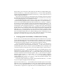
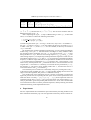
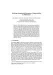
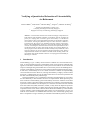
Fig. 1. Execution traces of a queue. Only the first trace (at the top) is linearizable. The second
trace is not linearizable, but is 1-quasi linearizable. The third trace is only 2-quasi linearizable.
Example 1. For a bounded queue that stores a set X of non-zero data items, we have
Domain(queue) = {enq.x, deq.x, deq.0 | x ∈ X}, where enq.x denotes the enqueue
operation for data x, deq.x denotes the dequeue operation for data x, and deq.0 indicates that the queue is empty. We may define two subsets of Domain(queue):
d1 = {enq.y | y ∈ Y } ,
d2 = {deq.y | y ∈ Y } .
Let D = {d1 , d2 }, where d1 is the subset of deq events and d2 is the subset of enq
events. The distance between σ and σ ′ , after being projected to subsets d1 and d2 ,
is defined as ∆(σ|d1 , σ ′ |d2 ). If we require that the enq calls follow the FIFO order
and the deq calls be out-of-order by at most K steps, the quasi-linearization factor
Q{queue} : D → N is defined as follows:
Q{queue} (d1 ) = 0 ,
Q{queue} (d2 ) = K .
Definition 4 (Quasi Linearizability). Given a model M = (O = {o1 , . . . , ok }, initO ,
P = {p1 , . . . , pn }). Let H be the behavior of M. M is quasi linearizable under the
quasi factor QO : D → N if for any history σ in H, there exists a sequential permutation π of σ such that
– for every op1 and op2 in σ, if op1 <σ op2 , then op1 <π op2 (i.e., π respects the
run-time ordering of operations), and
– for each object oi (1 ≤ i ≤ k), there exists another sequential permutation π ′ of π
such that
1. π ′|oi is a legal sequential history (i.e., π ′ respects the sequential specification
of the objects) and
2. ∆((π|oi )|d , (π ′|oi )|d ) ≤ QO (d) for all d ∈ D.
This definition subsumes the definition for linearizability because, if the quasi factor
is QO (d) = 0 for all d ∈ D, then the objects behaves as a standard linearizable data
structure, e.g., a FIFO queue.
Example 2. Consider the concurrent execution of a queue as shown in the Fig. 1. In the
first part, it is clear that the execution is linearizable, because it is a valid permutation
of the sequential history where Enq(Y) takes effect before Deq(X). The second part
5
is not linearizable, because the first dequeue operation is Deq(Y) but the first enqueue
operation is Enq(X). However, it is interesting to note that the second history is not
far from a linearizable history, since swapping the order of the two dequeue events
would make it linearizable. Therefore, flexibility is provided in dequeue events to allow
them to be reordered. Similarly, for the third part, if the quasi factor is 0 (no out-oforder execution) or 1 (out-of-order by at most 1 step), then the history is not quasi
linearizable. However, if the quasi factor is 2 (out-of-order by at most 2 steps), then the
third history in Fig.1 is considered as quasi linearizable.
2.3 Linearizability as Refinement
Linearizability is defined in terms of the invocations and responses of high-level operations. In a real concurrent program, the high-level operations are implemented by algorithms on concrete shared data structures, e.g., a linked list that implements a shared
stack object [18]. Therefore, the execution of high-level operations may have complicated interleaving of low-level actions. Linearizability of a concrete concurrent algorithm
requires that, despite low-level interleaving, the history of high-level invocation and response actions still has a sequential permutation that respects both the run-time ordering
among operations and the sequential specification of the objects.
For verifying standard (but not quasi) linearizability, an existing method [7, 8] can
be used to check whether a real concurrent algorithm (we refer as implementation in this
work) refines the high-level linearizable requirement (we refer as specification in this
work). In this case, the behaviors of the implementation and the specification are modeled as labeled transition systems (LTSs), and the refinement checking is accomplished
by using explicit state model checking.
Definition 5 (Labeled Transition System). A Labeled Transition System (LTS) is a
tuple L = (S, init, Act, →) where S is a finite set of states; init ∈ S is an initial state;
Act is a finite set of actions; and → ⊆ S × Act × S is a labeled transition relation.
α
For simplicity, we write s → s′ to denote (s, α, s′ ) ∈ →. The set of enabled actions
α
at s is enabled(s) = {α ∈ Act | ∃s′ ∈ S. s → s′ }. A path π of L is a sequence of
alternating states and actions, starting and ending with states π = hs0 , α1 , s1 , α2 , · · · i
αi+1
such that s0 = init and si → si+1 for all i. If π is finite, then |π| denotes the number
of transitions in π. A path can also be infinite, i.e., containing infinite number of actions.
Since the number of states are finite, infinite paths are paths containing loops. The set
of all possible paths for L is written as paths(L).
A transition label can be either a visible action or an invisible one. Given an LTS
L, the set of visible actions in L is denoted by visL and the set of invisible actions
is denoted by invisL . A τ -transition is a transition labeled with an invisible action. A
state s′ is reachable from state s if there exists a path that starts from s and ends with
∗
α
s′ , denoted by s ⇒ s′ . The set of τ -successors is τ (s) = {s′ ∈ S | s → s′ ∧ α ∈
invisL }. The set of states reachable from s by performing zero or more τ transitions,
denoted as τ ∗ (s), can be obtained by repeatedly computing the τ -successors starting
τ∗
from s until a fixed point is reached. We write s → s′ iff s′ is reachable from s via
only τ -transitions, i.e., there exists a path hs0 , α1 , s1 , α2 , · · · , sn i such that s0 = s,
αi+1
sn = s′ and si → si+1 ∧ αi+1 ∈ invisL for all i . Given a path π, we can obtain
6
1
a
2
3
5
a
4
b
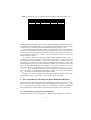
Fig. 2. An LTS example
a sequence of visible actions by omitting states and invisible actions. The sequence,
denoted as trace(π), is a trace of L. The set of all traces of L, is written as traces(L)
= {trace(π) | π ∈ paths(L)}.
LTSs can often be shown graphically, e.g., Fig. 2 shows an example LTS, where
invisible transition labels are omitted for simplicity. We define the refinement relation
between two LTSs, usually called trace refinement, as follows.
Definition 6 (Refinement). Let L1 and L2 be two LTSs. L1 refines L2 , written as
L1 ⊒T L2 iff traces(L1 ) ⊆ traces(L2 ).
⊓
⊔
In [7], we have shown that if Limpl is an implementation LTS and Lspec is the LTS
of the linearizable specification, then Limpl is linearizable if and only if Limpl ⊒T
Lspec .
Algorithm 1 shows the pseudo code of the refinement checking procedure in [7, 8].
Assume that Limpl refines Mspec , then for each reachable transition in Mimpl , denoted
e
e
as impl → impl′ , there must exist a reachable transition in Lspec , denoted as spec →
′
spec . Therefore, the procedure starts with the pair of initial states of the two models,
and repeatedly checks whether their have matching successor states. If the answer is no,
the check at Lines 6-8 would fail, meaning that Limpl is not linearizable. Otherwise, for
each pair of immediate successor states (impl′ , spec′ ), we add the pair to the pending
list. The entire procedure continues until either (1) a non-matching transition in Limpl
is found at Lines 6-8, or (2) all pairs of reachable states are checked, in which case
Limpl is proved to be linearizable.
In Algorithm 1, the subroutine next(impl, spec) is crucially important. It takes the
current states of Limpl and Lspec as input, and returns a set of state pairs of the form
(impl′ , spec′ ). Here each pair (impl′ , spec′ ) is one of the immediate successor state
pairs of (impl, spec). They are defined as follows:
τ
1. if impl −
→ impl′ , where τ is an internal event, then let spec′ = spec;
e
e
2. if impl −
→ impl′ , where e is a method call event, then spec −
→ spec′ ;
We have assumed, without loss of generality, that the specification model Lspec is deterministic. If the original specification model is nondeterministic, we can always apply
standard subset construction (of DFAs) to make it deterministic.
3 Verifying Quasi Linearizability: The Overview
Our verification problem is defined as follows: Given an implementation model Mimpl ,
a specification model Mspec , and a quasi factor QO , decide whether Mimpl is quasi
linearizable with respect to Mspec under the quasi factor QO .
7
Algorithm 1 Standard Refinement Checking
1:
2:
3:
4:
5:
6:
7:
8:
9:
10:
11:
12:
13:
14:
15:
16:
Procedure Check-Refinement(impl, spec)
checked := ∅
pending.push((initimpl , initspec ))
while pending 6= ∅ do
(impl, spec) := pending.pop()
if enabled(impl) 6⊆ enabled(spec) then
return false
end if
checked := checked ∪{(impl, spec)}
for all (impl′ , spec′ ) ∈ next(impl, spec) do
if (impl′ , spec′ ) ∈
/ checked then
pending.push((impl′ , spec′ ))
end if
end for
end while
return true
Sequential
Specification
Concurrent
Implementation
Sequential
Specification
QF
Concurrent
Implementation
QF
Create Manually
Relaxing the
Transitions
On Demand
Quasi−Lin Spec
Model
New Checking Algorithm
Standard Refinement Checking
(Impl vs. Q−Lin Spec)
Quasi Refinement Checking
(Impl vs. Spec)
Yes/No
Yes/No
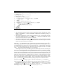
Fig. 3. Verifying quasi linearizability: manual approach (left) and automated approach (right).
The straightforward approach for solving the problem is to leverage the procedure
in Algorithm 1. However, since the procedure checks for standard refinement relation,
not quasi refinement relation, the user has to manually construct a relaxed specification
′
model, denoted Mspec
, based on the given specification model Mspec and the quasi
factor QO . This so-called manual approach is illustrated by Fig. 3 (left). The relaxed
′
specification model Mspec
must be able to produce all histories that can be produced
by Mspec , as well as the new histories that are allowed under the relaxed consistency
condition in Definition 4.
Unfortunately, there is no systematic method, or general guideline, on constructing
′
such relaxed specification models. Each Mspec
may be different depending on the type
of data structures to be checked. And there is significant amount of creativity required
during the process, to make sure that the new specification model is both simple enough
and permissive enough. For example, to verify that a K-segmented queue [3] is quasi
linearizable, we can create a relaxed specification model whose dequeue method ran8
domly removes one of the first K data items from the otherwise standard FIFO queue.
′
This new model Mspec
will be more complex than Mspec , but can still be significantly
simpler than the full-fledged implementation model Mimpl , which requires the use of a
complex segmented linked list.
Since the focus of this paper is on designing a fully automated verification method,
we shall briefly illustrate the manual approach in Section 4, and then focus on developing an automated approach in the subsequent sections.
Our automated approach is shown in Fig. 3 (right). It is based on designing a new
refinement checking algorithm that, in contrast to Algorithm 1, can directly check a relaxed version of the standard refinement relation between Mimpl and Mspec . Therefore,
′′
the user does not need to manually construct the relaxed specification model Mspec
. Instead, inside the new refinement checking procedure, we systematically extend states
and transitions of the specification model Mspec so that the new states and transitions
′
as required by Mspec
are added on the fly. This would lead to the inclusion of a bounded
degree of out-of-order execution on the relevant subset of operations as defined by the
quasi factor QO . A main advantage of our new method is that the procedure is fully
automated, thereby avoiding the user intervention, as well as the potential errors that
may be introduced during the user’s manual modeling process. Furthermore, by exploring the relaxed transitions on a need-to basis, rather than upfront as in the manual
approach, we can reduce the number of states that need to be checked.
4 Verifying Quasi Linearizability via Refinement Checking
In this section, we will briefly describe the manual approach and then focus on presenting the automated approach in the subsequent sections. Although we do not intend to
promote the manual approach – since it is labor-intensive and error prune – this section
will illustrate the intuitions behind our fully automated verification method.
Given the specification model Mspec and the quasi factor QO , we show how to
′
manually construct the relaxed specification model Mspec
in this section. We use the
standard FIFO queue and two versions of quasi linearizable queues as examples. The
construction needs to be tailored case by case for the different types of data structures.
Specification Model Mspec : The standard FIFO queue with a bounded capacity can be
implemented by using a linked list, where deq operation removes a data item at one
end of the list called the head node, and enq operation adds a data item at the other end
of the list called the tail node. When the queue is full, enq does not have any impact.
When the queue is empty, deq returns NULL. As an example, consider a sequence
of four enqueue events enq(1), enq(2), enq(3), enq(4), the subsequent dequeue
events would be deq.1, deq.2, deq.3, deq.4, which obey the FIFO semantics. This
is illustrated by the first history H1-a in Fig. 5.
In the PAT model checking environment, the specification model Mspec is written
in a process algebra language, named CSP# [19].
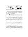
Implementation Model Mimpl : The bounded quasi linearizable queue can be implemented by using a segmented linked list. This is the original algorithm proposed by
Afek et al. [3]. A segmented linked list is a linked list where each list node can hold
K data items, as opposed to a single data item in the standard linked list. As shown
9
H1-a
------enq(1)
enq(2)
enq(3)
enq(4)
deq()=1
deq()=2
deq()=3
deq()=4
-------
H1-b
------enq(1)
enq(2)
enq(3)
enq(4)
deq()=1
deq()=2
deq()=4
deq()=3
-------
H1-a
------enq(1)
enq(2)
enq(3)
enq(4)
deq()=2
deq()=1
deq()=3
deq()=4
-------
H1-b
------enq(1)
enq(2)
enq(3)
enq(4)
deq()=2
deq()=1
deq()=4
deq()=3
-------
Fig. 5. Valid histories of a 1-quasi linearizable queue, meaning that deq can be outof-order by 1. The first deq randomly returns a value from the set {1, 2} and the
second deq returns the remaining one.
Then the third deq randomly returns a value from the set {3, 4} and the forth deq returns the remaining one.
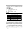
Fig. 4. Implementations of a 4-quasi queue
in Fig. 4 (lower half), these K data items form a segment, in which the data slots are
numbered as 1, 2, . . ., K. In general, the segment size needs to be set to (QF + 1),
where QF is the maximum number of out-of-order execution steps. The example in
Fig. 4 has the quasi factor set to 3, meaning that a deq operation can be executed out
of order by at most 3 steps. Consequently, the size of each segment is set to (3+1)=4.
Since Q{queue} (Denq ) = 0, meaning that the enq operations cannot be reordered, the
data items are enqueued regularly in the empty slots of one segment, before the head
points to the next segment. But for deq operations, we randomly remove one existing
data item from the current segment.
′
Relaxed Specification Model Mspec
: Not all execution traces of Mimpl are traces of
Mspec . In Fig. 5, histories other than H1-a are not linearizable. However, they are all
quasi linearizable under the quasi factor 1. They may be produced by a segmented
queue where the segment size is (1+1)=2. To verify that Mimpl is quasi linearizable, we
′
, which includes not only all histories of Mspec but also the
construct a new model Mspec
histories that are allowed only under the relaxed consistency condition. In this example,
we choose to construct the new model by slightly modifying the standard FIFO queue.
This is illustrated in Fig. 4 (upper half), where the first K data items are grouped into a
cluster. Within the cluster, the deq operation may remove any of the k data items based
on randomization. Only after the first k data items in the cluster are retrieved, will the
deq move to the next k data items (a new cluster). The external behavior of this model is
expected to match that of the segmented queue in Mimpl : both are 1-quasi linearizable.
′
Checking Refinement Relation: Once Mspec
is available, checking whether Mimpl re′
fines Mspec is straightforward by using Algorithm 1. For the segmented queue imple′
mentation [3], we have manually constructed Mspec
and checked the refinement relation
in the PAT model checking environment. Our experimental results are summarized in
Table 1. Column 1 shows the different quasi factors. Column 2 shows the number of
segments – the capacity of the queue is (QF + 1) × Seg. Column 3 shows the refinement checking time in seconds. Column 4 shows the total number of visited states
10
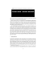
Table 1. Experimental results for standard refinement checking. MOut means memory-out.
Quasi Factor #. Segment Verification Time (s) #. Visited State #. Transition
1
1
0.1
423
778
1
2
0.1
2310
4458
1
3
0.1
8002
15213
1
4
0.4
22327
41660
1
5
0.9
55173
101443
1
6
2.0
126547
230259
1
10
55.9
2488052
4421583
1
15
MOut
2
1
0.6
26605
58281
2
2
12.6
456397
970960
2
3
130.7
4484213
8742485
2
4
MOut
3
1
8.8
284484
638684
3
2
MOut
4
1
124.4
3432702
7906856
4
2
MOut
-
during refinement checking. Column 5 shows the total number of state transitions activated during refinement checking. The experiments are conducted on a computer with
an Intel Core-i7, 2.5 GHz processor and 8 GB RAM running Ubuntu 10.04.
The experimental results in Table 1 show an exponential increase in the verification
time when we increase the size of the queue or the quasi factor. This is inevitable since
the size of the state space grows exponentially. However, this method requires the us′
er to manually construct Mspec
, which is a severe limitation because it is often labor
intensive and error prone.
For example, consider the seemingly simple random dequeued model in Fig. 4.
A subtle error would be introduced if we do not use the cluster to restrict the set of
data items that can be removed by deq operation. Assume that deq always returns one
of the first k data items in the current queue. Although it appears to be correct, such
implementation will not be k-quasi linearizable, because it is possible for some data
item to be over-taken indefinitely. For example, if every time deq chooses the second
data item in the list, we will have the following deq sequence: deq.2, deq.3, deq.4,
. . ., deq.1, where the dequeue of value 1 can be delayed by an arbitrarily long time.
This is no longer a 1-quasi linearizable queue. In other words, if the user construct
′
Mspec
incorrectly, the verification result becomes invalid.
Therefore, we need to design a fully automated method to directly verify quasi
linearizability of Mimpl against Mspec under the given quasi factor QF .
5 New Algorithm for Checking the Quasi Refinement Relation
We shall start with the standard refinement checking procedure in Algorithm 1 and extend it to directly check a relaxed version of the refinement relation between Mimpl and
Mspec under the given quasi factor. The idea is to establish the simulation relationship
from specification to implementation while allowing relaxation of the specification.
5.1 Linearizability Checking via Quasi Refinement
The new procedure, shown in Algorithm 2, is different from Algorithm 1 as follows:
11
Algorithm 2 Quasi Refinement Checking
1:
2:
3:
4:
5:
6:
7:
8:
9:
10:
11:
12:
13:
14:
15:
16:
Procedure Check-Quasi-Refinement(impl, spec, QF )
checked := ∅
pending.enqueue((initimpl , initspec ))
while pending 6= ∅ do
(impl, spec) := pending.dequeue()
if enabled(impl) 6⊆ enabled relaxed(spec, QF ) then
return false
end if
checked := checked ∪{(impl, spec)}
for all (impl′ , spec′ ) ∈ next relaxed(impl, spec, QF ) do
if (impl′ , spec′ ) ∈
/ checked then
pending.enqueue((impl′ , spec′ ))
end if
end for
end while
return true
1. We customize pending to make the state exploration follow a breadth-first search
(BFS). In Algorithm 1, it can be either BFS or DFS based on whether pending is a
queue or stack.
2. We replace enabled(spec) with enabled relaxed(spec,QF). It will return not only
the events enabled at current spec state in Mspec , but also the additional events
allowed under the relaxed consistency condition.
3. We replace next(impl,spec) with next relaxed(impl,spec,QF). It will return not only
the successor state pairs in the original models, but also the additional pairs allowed
under the relaxed consistency condition.
′
Conceptually, it is equivalent to first constructing a relaxed specification model Mspec
from (Mspec , QF ) and then computing the enabled(spec) and next(impl,spec) on this
′
new model. However, in this case, we are constructing Mspec
automatically, without the
user’s intervention. Furthermore, the additional states and edges that need to be added
′
to Mspec
are processed incrementally, on a need-to basis.
At the high level, the new procedure performs a BFS exploration for the state pair
(impl, spec), where impl is the state of implementation and spec is a state of specification. The initial implementation and specification events are enqueued into pending
and each time we go through the while-loop, we dequeue from pending a state pair, and
check if all events enabled at state impl match with some events enabled at state spec
under the relaxed consistency condition (Line 6). If there is any mismatch, the check
fails and we can return a counterexample showing how the violation happens. Otherwise, we continue until pending is empty. Lines 10-14 explore the new successor state
pairs, by invoking next relaxed and add to pending if they have not been checked.
Subroutine enabled relaxed(spec,QF): It takes the current state spec of model Mspec ,
along with the quasi factor QF , and generates all events that are enabled at state spec.
Consider the graph in Fig. 6 as Mspec . Without relaxation, enabled(s1 )={e1 }. This
is equivalent to enabled relaxed(s1 , 0). However, when QF = 1, according to the
dotted edges in Fig. 7, the set enabled relaxed(s1 , 1)={e1 , e2 , e3 }.
12
e1
s7
e4
e1
s1
s2
e2
s3
e4
e3
e3
s1
s4
e6
e5
e1
e2
s6
s5
s2
e2
e1
s3
e3
s4
e6
e5
s5
Fig. 7. Specification model after adding relaxed edges for state s1 and quasi factor 1.
Fig. 6. Specification model before the addition of relaxed transitions for state s1 .
The reason why e2 and e3 become enabled is as follows: before relaxation, starting
at state s1 , there are two length-2 event sequences σ1 = e1 , e2 and σ2 = e1 , e3 . When
QF = 1, it means an event can be out-of-order by at most 1 step. Therefore, the permutation of σ1 is π1 = e2 , e1 , and the permutation of σ2 is π2 = e3 , e1 . In other words,
at state s1 , events e2 , e3 can also be executed.
Subroutine next relaxed(impl, spec, QF ): It takes the current state impl of Mimpl
and the current state spec of Mspec as input, and returns a set of state pairs of the form
(impl′ , spec′ ). Similar to the definition of next(impl, spec) in Section 2, we define
each pair (impl′ , spec′ ) as follows:
τ
1. if impl −
→ impl′ , where τ is an internal event, then let spec′ = spec;
e
e
2. if impl −
→ impl′ , where e is a method call event, then spec −
→ spec′ where event
e ∈ enabled relaxed(spec, QF ) is enabled at spec after relaxation.
For example, when spec = s1 in Fig. 6, and the quasi factor is set to 1 – meaning that the event at state s1 can be out-of-order by at most one step – the procedure
next relaxed(impl,s1, 1) would return not only (impl′ , s2 ), but also (impl′ , s6 ) and
(impl′ , s7 ), as indicated by the dotted edges in Fig. 7. The detailed algorithm for generation of the relaxed next states in specification is described in Section 5.2.
5.2 Generation of Relaxed Specification
In this subsection, we show how to relax the specification Mspec by adding new states
and transitions – those that are allowed under the condition of quasi linearizability –
to form a new specification model. Notice that we accomplish this automatically, and
incrementally, on a need-to basis.
For each state spec in Mspec , we compute all the event sequences starting at spec
with the length (QF + 1). These event sequences can be computed by using a simple
graph traversal algorithm, e.g. a breadth first search.
Fig. 6 shows an example for the computation of these event sequences. The specification model Mspec has the following set of states {s1 , s2 , s3 , s4 , s5 }. Suppose that the
current state is s1 (in step 0), then the current frontier state set is {s1 }, and the current
event sequence is hs1 i. The results of each BFS step is shown in Table 2. In step 1, the
e1
s2 i. In step 2, the
frontier state set is {s2 }, and the event sequence becomes hs1 →
frontier state set is {s3 , s4 }, and the event sequence is split into two sequences. One is
13
Table 2. Specification Sequence Generation at State s1
BFS Steps
step 0
step 1
step 2
step 3
e
(Frontier)
{s1 }
{s2 }
{s3 , s4 }
{s5 , s2 , s1 }
EventSequences
hs1 i
e1
s2 i
hs1 →
e3
e1
e2
e1
s4 i
s2 →
s3 ihs1 →
s2 →
hs1 →
e4
e3
e1
e6
e3
e1
e2
e1
s1 i
s4 →
s2 →
s2 ihs1 →
s4 →
hs1 → s2 → s3 , s5 ihs1 → s2 →
e
e
e
3
1
2
1
s4 i. The traversal continues until the
s2 →
s3 i and the other is hs1 →
s2 →
hs1 →
BFS depth reaches (QF + 1).
After completing the (QF + 1) steps of BFS starting at state spec, as described
above, we are able to evaluate the following subroutines:
– enabled relaxed(spec, QF ),
– next relaxed(impl, spec, QF ).
Consider the quasi factor QF = 0 in Fig. 6. In this case, only event e1 is enabled at s1 .
For QF = 1, however, events e2 , e3 are also enabled, as shown by the results at step 2
in Table 2. For QF = 2, events e4 , e5 , e5 are also enabled, as shown by the results at
step 3 in the table.
We transform the original specification model in Fig. 6 to the relaxed specification
model in Fig. 7 for QF = 1. The dotted states and edges are newly added to reflect
the relaxation. More specifically, for QF = 1, we will reach (QF + 1) = 2 steps
during the BFS. At step 2, there are two existing sequences {e1 , e2 } and {e1 , e3 }. For
each existing sequence, we compute all possible permutation sequences. In this case, the
permutation sequences are {e2 , e1 } and {e3 , e1 }. For each newly generated permutation
sequence, we add new edges and states to the specification model. From an initial state
s1 , if we follow the new permutation {e2 , e1 }, as shown in Fig. 7, the transition e2 will
lead to newly formed pseudo state s6 and from this state it is reconnected back to the
original state s3 via transition e1 . Similarly, if we follow the new permutation {e3 , e1 },
the transition e3 will lead to newly formed pseudo state s7 , and from this state it is
reconnected back to state s4 via transition e1 .
This relaxation process needs to be conducted by using every existing state of Mspec
as the starting point (for BFS up to QF + 1 steps) and then adding the new states and
edges. In our new algorithm, this process is conducted on the fly.
The pseudo code of this relaxation process is shown in Algorithm 3 explains the
high level pseudo-code for expanding the state space for the current specification state
under the check. Let SEQ = {seq1 , seq2 , seq3 , ..., seqk } be the sequences which are
reachable from the state s0 in Mspec for a given quasi factor QF . Each sequence seq ∈
SEQ is permuted to get all the possible paths for that trace. A new state is formed with
a new transition for each event in the permuted sequences, thereby allowing the relaxed
refinement checking of the implementation trace.
6 Experiments
We have implemented and evaluated the quasi linearizability checking method in the
PAT verification framework [14]. Our new algorithm can directly check a relaxed ver14
Algorithm 3 Pseudo-code for Expanding Specification Under Check
1: Let s0 be a specification state and QF be the quasi factor
2: Let SEQ = {seq1 , seq2 , seq3 , · · · , seqk } be the set of all possible event sequences reachable from s0 in Mspec such that for 1 ≤ i ≤ k, the length of seqi is less than or equal to
QF + 1
3: for all seq in SEQ do
4:
Let PERMUT SEQ be the set of permutations of seq
5:
for all perm in PERMUT SEQ do
6:
Let perm = he1 , e2 , · · · , en i
7:
Let sn be the specification state reached from s0 via seq
8:
if perm is not equal to seq then
9:
for all ei where 1 ≤ i < n do
10:
Create a new state si and a new transition from si−1 to si via event ei
11:
end for
12:
Create a new transition from sn−1 to sn via en
13:
end if
14:
end for
15: end for
Table 3. Statistics of Benchmark Examples
Class
Quasi Queue (3)
Quasi Queue (6)
Quasi Queue (9)
Queue buggy1
Queue buggy2
Lin. Queue
Q. Priority Queue (3)
Q. Priority Queue (6)
Q. Priority Queue (9)
Priority Queue buggy
Lin. Stack
Description
Segmented linked list implementation (size=3)
Segmented linked list implementation (size=6)
Segmented linked list implementation (size=9)
Segmented queue with a bug (Dequeue on the empty
queue may erroneously change current segment)
Segmented queue with a bug (Dequeue may get
value from a wrong segment)
A linearizable (hence quasi) implementation
Segmented linked list implementation (size=3)
Segmented linked list implementation (size=6)
Segmented linked list implementation (size=9)
Segmented priority queue (Dequeue on the empty
priority queue may change current segment)
A linearizable (hence quasi) implementation
Linearizable Quasi Lin.
No
Yes
No
Yes
No
Yes
No
No
No
No
Yes
No
No
No
No
Yes
Yes
Yes
Yes
No
Yes
Yes
sion of the refinement relation. This new algorithm subsumes the standard refinement checking procedure that has already been implemented in PAT. In particular, when
QF = 0, our new procedure degenerates to the standard refinement checking procedure. When QF > 0, our new procedure has the added capability of checking for the
quantitatively relaxed refinement relation. Our algorithm can directly handle the implementation model Mimpl , the standard (not quasi) specification model Mspec , and the
quasi factor QF , thereby completely avoiding the user’s intervention.
We have evaluated our new algorithm on a set of models of standard and quasi linearizable concurrent data structures [3, 5, 6, 4], including queues, stacks, quasi queues,
quasi stacks, and quasi priority queues. For each data structure, there can be several
variants, each of which has a slightly different implementation. In addition to the implementations that are known to be linearizable and quasi linearizable, we also have
versions which initially were thought to be correct, but were subsequently proved to
be buggy by our verification tool. The characteristics of all benchmark examples are
shown in Table 3. The first two columns list the name of the concurrent data structures
15
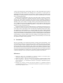
Table 4. Results for Checking Quasi Linearizability with 2 threads and QF = 2
Class
Quasi Queue(3)
Quasi Queue(6)
Quasi Queue(9)
Queue buggy1
Queue buggy2
Lin. Queue
Q. Priority Queue(3)
Q. Priority Queue(6)
Q. Priority Queue(9)
Priority Queue buggy
Lin. Stack
Verification Time (s) Number of Visited States Number of Visited Transitions
7.2
126,810
248,122
21.2
237,760
468,461
114.5
1,741,921
3,424,280
0.4
1,204
809
0.1
345
345
5.5
240,583
121,548
12.2
106,385
195,235
34.3
472,981
918,530
198.4
1,478,045
2,905,016
5.4
894
894
0.2
2,690
6,896
and a short description of the implementation. The next two columns show whether the
implementation is linearizable and quasi linearizable.
Table 4 shows the results of the experiments. The experiments are conducted on a
computer with an Intel Core-i7, 2.5 GHz processor and 8 GB RAM running Ubuntu
10.04. The first column shows the statistics of the test program, including the name
and the size of benchmark. The next three columns show the runtime performance,
consisting of the verification time in seconds, the total number of visited states, and the
total number of transitions made. The number of states and the running time for each
of the models increase with the data size.
For 3 segmented quasi queue with quasi factor 2, the verification completes in 7.2
seconds. It is much faster than the first approach presented in Section 4, where the same
setting requires 130.7 seconds for the verification. Subsequently, as the size increases,
the time to verify the quasi queue increases. For queue with size 6 and 9, verification
is completed in 21.2 seconds and 114.5 seconds, respectively. For the priority queues
where enqueue and dequeue operations are performed based on the priority, the verification time is higher than the regular quasi queue. Also, it is important to note that
the counterexample is produced with exploration of only part of the state space for the
buggy models. The verification time is much faster for the buggy queue, which shows
that our approach is effective if the quasi linearizability is not satisfied. In all test cases,
our method was able to correctly verify quasi linearizability of the implementation or
detect the violations.
7 Related Work
In the literature, although there exists a large body of work on formally verifying linearizability in models of data structure implementations, none of them can verify quasi
linearizability. For example, Liu et al. [7, 8] use a process algebra based tool to verify
that an implementation model refines a specification model – the refinement relation
implies linearizability. Vechev et al. [9] use the SPIN model checker to verify linearizability in a Promela model. Cerný et al. [10] use automated abstractions together with
model checking to verify linearizability properties. There also exists some work on
proving linearizability by constructing mechanical proofs, often with significant manual intervention (e.g., [12, 13]).
There are also runtime verification algorithms such as Line-Up [11], which can
directly check the actual source code implementation but for violations on bounded ex16
ecutions and deterministic linearizability. However, quasi linearizable data structures
are inherently nondeterministic. For example, the deq operation in a quasi queue implementation may choose to return any of the first k items in a queue. To the best of our
knowledge, no existing method can directly verify quasi linearizability for execution
traces of unbounded length.
Besides (quasi) linearizability, there also exist many other consistency conditions for concurrent computations, including sequential consistency [20], quiescent consistency [21], and eventual consistency [22]. Some of these consistency conditions in
principle may be used for checking the correctness of data structure implementations,
although so far, none of them is as widely used as (quasi) linearizability. These consistency conditions do not involve quantitative aspects of the properties. We believe that
it is possible to extend our refinement algorithm to verify some of these properties.
However, we leave it for future work.
Outside the domain of concurrent data structures, serializability and atomicity are two popular correctness properties for concurrent programs, especially at the application
level. There exists a large body of work on both static and dynamic analysis for detecting violations of such properties (e.g., [23, 24] and [25–28]). These existing methods
are different from ours because they are checking different properties. Although atomicity and serializability are fairly general correctness conditions, they have been applied
mostly to the correctness of shared memory accesses at the load/store instruction level.
Linearizability, in contrast, defines correctness condition at the method call level. Furthermore, existing methods for checking atomicity and serializability do not deal with
the quantitative aspects of the properties.
8 Conclusions
We have presented a new method for formally verifying quasi linearizability of the
implementation models of concurrent data structures. We have explored two approaches, one of which is based on manual construction of the relaxed specification model,
whereas the other is fully automated, and is based on checking a relaxed version of
the refinement relation between the implementation model and the specification model.
We believe that the automated refinement checking algorithm can be further optimized
to improve performance. For future work, we plan to incorporate advanced state space
reduction techniques such as symmetry reduction and partial order reduction.
References
1. Herlihy, M., Wing, J.M.: Linearizability: A correctness condition for concurrent objects.
ACM Trans. Program. Lang. Syst. 12(3) (1990) 463–492
2. Herlihy, M., Shavit, N.: The art of multiprocessor programming. Morgan Kaufmann (2008)
3. Afek, Y., Korland, G., Yanovsky, E.: Quasi-Linearizability: Relaxed consistency for improved concurrency. In: International Conference on Principles of Distributed Systems.
(2010) 395–410
4. Henzinger, T.A., Sezgin, A., Kirsch, C.M., Payer, H., Sokolova, A.: Quantitative relaxation
of concurrent data structures. In: ACM SIGACT-SIGPLAN Symposium on Principles of
Programming Languages. (2013)
17
5. Kirsch, C.M., Payer, H., Röck, H., Sokolova, A.: Performance, scalability, and semantics
of concurrent fifo queues. In: International Conference on Algorithms and Architectures for
Parallel Processing. (2012) 273–287
6. Payer, H., Röck, H., Kirsch, C.M., Sokolova, A.: Scalability versus semantics of concurrent
fifo queues. In: ACM Symposium on Principles of Distributed Computing. (2011) 331–332
7. Liu, Y., Chen, W., Liu, Y.A., Sun, J.: Model checking linearizability via refinement. In:
Proceedings of the 2nd World Congress on Formal Methods, Berlin, Heidelberg, SpringerVerlag (2009) 321–337
8. Liu, Y., Chen, W., Liu, Y., Zhang, S., Sun, J., Dong, J.S.: Verifying linearizability via optimized refinement checking. IEEE Transactions on Software Engineering (2013)
9. Vechev, M.T., Yahav, E., Yorsh, G.: Experience with model checking linearizability. In:
International SPIN Workshop on Model Checking Software. (2009) 261–278
10. Cerný, P., Radhakrishna, A., Zufferey, D., Chaudhuri, S., Alur, R.: Model checking of linearizability of concurrent list implementations. In: International Conference on Computer
Aided Verification. (2010) 465–479
11. Burckhardt, S., Dern, C., Musuvathi, M., Tan, R.: Line-up: a complete and automatic linearizability checker. In: ACM SIGPLAN Conference on Programming Language Design
and Implementation. (2010) 330–340
12. Vafeiadis, V.: Shape-value abstraction for verifying linearizability. In: International Conference on Verification, Model Checking, and Abstract Interpretation, Berlin, Heidelberg,
Springer-Verlag (2009) 335–348
13. Vafeiadis, V., Herlihy, M., Hoare, T., Shapiro, M.: Proving correctness of highly-concurrent
linearisable objects. In: ACM SIGPLAN symposium on Principles and practice of parallel
programming, New York, NY, USA, ACM (2006) 129–136
14. Sun, J., Liu, Y., Dong, J.S., Pang, J.: PAT: Towards Flexible Verification under Fairness. In:
Proceedings of the 21th International Conference on Computer Aided Verification. Volume
5643 of Lecture Notes in Computer Science. (2009) 709–714
15. Hoare, C.A.R.: Communicating Sequential Processes. Prentice Hall, Englewood Cliffs, NJ
(1985)
16. Lynch, N.: Distributed Algorithms. Morgan Kaufmann (1997)
17. Attiya, H., Welch, J.: Distributed Computing: Fundamentals, Simulations, and Advanced
Topics. 2nd edn. John Wiley & Sons, Inc., Publication (2004)
18. Treiber, R.K.: Systems Programming: Coping with Parallelism. Technical Report RJ 5118,
IBM Almaden Research Center (1986)
19. Sun, J., Liu, Y., Dong, J.S., Chen, C.: Integrating specification and programs for system
modeling and verification. In: Proceedings of the third IEEE International Symposium on
Theoretical Aspects of Software Engineering. (2009) 127–135
20. Lamport, L.: How to make a multiprocessor computer that correctly executes multiprocess
programs. IEEE Trans. Computers 28(9) (1979) 690–691
21. Aspnes, J., Herlihy, M., Shavit, N.: Counting networks. J. ACM 41(5) (1994) 1020–1048
22. Vogels, W.: Eventually consistent. Commun. ACM 52(1) (2009) 40–44
23. Flanagan, C., Qadeer, S.: A type and effect system for atomicity. In: ACM SIGPLAN
Conference on Programming Language Design and Implementation. (2003) 338–349
24. Farzan, A., Madhusudan, P.: Causal atomicity. In: International Conference on Computer
Aided Verification. (2006) 315–328
25. Wang, L., Stoller, S.D.: Runtime analysis of atomicity for multithreaded programs. IEEE
Trans. Software Eng. 32(2) (2006) 93–110
26. Farzan, A., Madhusudan, P.: Monitoring atomicity in concurrent programs. In: International
Conference on Computer Aided Verification. (2008) 52–65
27. Sadowski, C., Freund, S.N., Flanagan, C.: Singletrack: A dynamic determinism checker for
multithreaded programs. In: European Symposium on Programming. (2009) 394–409
28. Wang, C., Limaye, R., Ganai, M., Gupta, A.: Trace-based symbolic analysis for atomicity violations. In: International Conference on Tools and Algorithms for Construction and
Analysis of Systems. (2010) 328–342
18