1
T-AXI Blade V1.8 User Manual
Kevin Park & David Gutzwiller
05-30-09
1
Contents
1 Introduction
1.1 License Information . . . . .
1.2 Code Overview and Features
1.3 System Requirements . . . .
1.4 Installation . . . . . . . . . .
.
.
.
.
3
3
3
3
3
2 Program Interface
2.1 Program Initialization and Setup . . . . . . . . . . . . . . . . . . . . . . . . . . . . .
2.2 Main Program Window . . . . . . . . . . . . . . . . . . . . . . . . . . . . . . . . . .
2.3 Program Output Modes . . . . . . . . . . . . . . . . . . . . . . . . . . . . . . . . . .
4
4
5
7
.
.
.
.
.
.
.
.
.
.
.
.
.
.
.
.
.
.
.
.
.
.
.
.
.
.
.
.
.
.
.
.
.
.
.
.
.
.
.
.
.
.
.
.
.
.
.
.
.
.
.
.
.
.
.
.
.
.
.
.
.
.
.
.
.
.
.
.
.
.
.
.
.
.
.
.
.
.
.
.
.
.
.
.
.
.
.
.
.
.
.
.
.
.
.
.
.
.
.
.
.
.
.
.
.
.
.
.
.
.
.
.
.
.
.
.
.
.
.
.
3 Background
11
3.1 Nomenclature . . . . . . . . . . . . . . . . . . . . . . . . . . . . . . . . . . . . . . . . 11
3.2 Establishing a Coordinate System and Vector Triangles. . . . . . . . . . . . . . . . . 12
3.3 T-AXI Blade Theory of Operation . . . . . . . . . . . . . . . . . . . . . . . . . . . . 14
4 Example Analysis: EEE 3rd Stage Rotor
4.1 Background . . . . . . . . . . . . . . . . . . . . . . . . . . . . . . . . . . . . . . . . .
4.2 Problem Setup . . . . . . . . . . . . . . . . . . . . . . . . . . . . . . . . . . . . . . .
4.3 Step By Step Procedure . . . . . . . . . . . . . . . . . . . . . . . . . . . . . . . . . .
15
15
16
17
5 Bug Reporting and Additional Help
20
2
1
Introduction
1.1
License Information
T-Axi Blade is released under the GNU General Public License Version 3, 29 June 2007.
Please see the included file ”gpl license.txt” for information regarding reproduction and distribution.
1.2
Code Overview and Features
T-Axi Blade is a GUI based, free-vortex blade row design and visualization program. The primary
purpose of T-Axi Blade is to develop students’ physical understanding of key blade design features,
with a special emphasis on the relationship between velocity triangles and blade shapes. The
specific features of this code are summarized below.
• Support for axial and centrifugal compressor and turbine designs.
• GUI driven design and analysis.
• Detailed data output including vector triangles and values, cascade views for hub, pitch and
tip, Smith Charts, and Loading vs. Aspect Ratio charts.
• Formatted output of common turbomachinery equations, solved for the current blade row
design.
• Temperature dependant material database.
• Preliminary design stress analysis based on AN 2 values.
1.3
System Requirements
Operating System
Processor
Memory
Display
1.4
Windows 2000 / XP / Vista
Pentium 3 or faster recommended
256 MB or greater
1024 x 768 with 256 colors
Installation
T-Axi Blade and the related T-Axi Disk codes are available from the University of Cincinnati
GTSL website: http://GTSL.ase.uc.edu/T-AXI. Download the file BD SUITE.zip and extract
the entire package to a known location on your hard drive. The unzip process should create all of
the necessary files and folders. Input files are contained in the subdirectory named “INPUTS”, the
material database is located under “MATERIALS”, and documentation is located under “HELP”.
The user should be careful not to change the file structure of T-Axi Disk as it may render the
code inoperable. Double clicking on the TAXI BLADE V1 8.exe icon will load the T-Axi Blade
GUI.
3
2
2.1
Program Interface
Program Initialization and Setup
Upon execution of T-Axi Blade the user is presented with a splash screen showing copyright and
author information. Clicking on the “OK” button brings the user to the blade file loading menu.
The user should select a blade input file (.tri) from this prompt and then click “Open” to continue.
The default blade file is for a first stage axial compressor section, and will load automatically if
“Cancel” is pressed. This should be used if a input file has not been created yet.
The “Choose Interface Options” window appears after the selection of a valid blade input file.
This windows reads and presents the information from the .tri file chosen in the previous step.
Figure 1 shows this window. The user should investigate the options carefully before continuing.
Any changes to these conditions should be made at this step. Clicking the “OK” will take the user
to the main T-Axi Blade window.
Figure 1: T-AXI Blade Interface Options Window.
4
2.2
Main Program Window
Figure 2 shows the main T-Axi Blade window. This window contains all of the controls needed to
design and analyze a blade and blade row. A short explanation of the controls marked with the
red numbers is shown below.
Figure 2: T-AXI Blade Main Window.
1. Phi (φ): Allows the user to change Phi (angle between the engine axis and the meridional)
at the leading edge (φLe ) and at the trailing edge (φT e ).
2. Vmle : Meridional velocity(m/s) at the leading edge. The ratio of velocities between the
leading and trailing edges is adjusted with the slider to the right.
3. R Pitch: Radius from engine centerline to the pitch of the blade, leading or trailing edge
respectively.
4. Mdot (ṁ): Sets the mass-flow rate across the stage in kilograms/second.
5. RPM: Sets the design speed RPM.
5
6. Eta rotor (ηrot ): Specifies rotor efficiency.
7. Delta TT (∆TT ): Specifies change in Total Temperature(Kelvin) across the rotor.
8. Alpha mle Pitch (αmle ): Specifies the angle(deg) between the velocity(m/s) of the fluid
entering the stage, and its meridional component at the leading edge.
9. Delta Z: Specifies the engine-axis length of the blade.
10. Blade Thickness: Sets the blade thickness at the hub(meters), with the slider to the right
setting the thickness at the tip.
11. Blades: Specifies the number of blades in the current row.
12. Save Inputs: Saves the input conditions to a .tri file.
13. View Selector: Changes the view between different options. Options are:
• Axial View: Displays an axial view of the blade along with relevant data and vector
triangles.
• Hub View: Displays a radial view of the hub cross-section of the blade row and all
relevant data and vector triangles.
• Pitch View: Same as Hub View, with data displayed changing to reflect pitch values.
• Tip View: Same as Hub View, with data displayed changing to reflect tip values.
• Data Printout: Text printout of input values and simulation output.
• Smith Chart: Smith Chart showing values for the hub, pitch and tip.
• Loading vs. AR: Loading vs. Aspect Ratio chart.
• Equations: Shows a formatted equations sheet, solved for the current design.
14. Material Menu: Drop-down menu for blade material selection. The menu consists of the
material files of the .dmat type, stored in the “\MATERIALS” folder. Default options include
several alloys such as INCONEL 706, INCONEL 718, and A286 to name a few.
15. Save Disk Output: Saves the blade geometry .dsk and flowpath dimensions for use in
T-AXI Disk to a .din file.
6
2.3
Program Output Modes
Figure 3 shows the axial view output from the T-AXI Blade main window. An overview of the
displayed data indicated with red numbers is given below.
Figure 3: T-AXI Blade Axial View.
1. Meridional Velocity (Vm ): This is the magnitude of the meridional velocity vector shown
in #6.
2. Radial Velocity (Vr ): This is the magnitude of the radial velocity vector shown in #6.
3. Axial Velocity (Vz ): This is the magnitude of the axial velocity vector shown in #6.
4. Phi (φ): This is the angle (deg) between the axial velocity vector, and the meridional velocity
vector.
5. Graphic: This is the graphical representation of the axial view of the blade.
6. Vector Triangle: This vector triangle represents the three flow components whose magnitudes are given: axial velocity, radial velocity, and meridional velocity.
7
Figure 4 shows the pitch view output option from the T-AXI Blade main window. An overview
of the data indicated with red numbers is shown below.
Figure 4: T-AXI Blade Pitch View.
1. Values Table: Table showing the magnitudes of the vectors and angles from the vector
triangles.
• Vm : Magnitude of meridional velocity, shown as vector #2.
• αm : Angle(deg) between meridional velocity(#2) and absolute velocity(#3).
• βm : Angle(deg) between meridional velocity(#2) and relative velocity of the flow as seen
by the blade row(#4).
• V: Magnitude of the absolute velocity, shown as vector #3.
• W: Magnitude of the relative velocity of the flow as seen by the blade row, shown as
vector #4.
• Vθ : Magnitude of tangential (swirl) velocity, shown as vector #5.
• Wθ : Magnitude of relative tangential (swirl) velocity of the flow as seen by the blade
row, shown as vector #6.
• U: Magnitude of velocity of the blade row, shown as vector #7.
• Mrel : Mach number of the flow seen by the blade row, shown as vector #4.
2. Meridonal Velocity: Velocity along the m’ cutplane.
8
3. True Velocity: Velocity of the flow as seen by an outside observer.
4. Relative Velocity: Flow velocity as seen by the blade row.
5. Tangential Velocity: Velocity component of the true velocity in the tangential direction
(swirl).
6. Relative Tangential Velocity: Velocity component of the relative velocity seen by the
blade row in the tangential direction.
7. Blade Row Velocity: Tangential velocity of the blade row at the radius specified (hub,
pitch, or tip).
8. Axial View Data: Data from the axial view including meridional, radial, and axial velocity
vectors.
9. Graphic: Cross-section of the blade row at the radius specified (hub, pitch, or tip).
Several other options are available for displaying the data output from T-AXI Blade. Figure 5
shows the Data Printout option available from the pull-down menu. There is also a Smith chart
and a Loading vs. Aspect Ratio chart available. A recent addition to T-Axi Blade is a formatted
printout of common turbomachinery equations, solved for the current blade design. This page
provides students with an easy way to find and fix mistakes in any hand calculations they are
performing in addition to the T-Axi Blade analysis.
Figure 5: T-AXI Blade Data Printout View.
9
Figure 6: T-AXI Blade Equation Printout.
Figure 7: T-AXI Blade Equation Printout.
10
3
3.1
Background
Nomenclature
T-AXI was created using the nomenclature shown below. There are however, many nomenclature
systems in use throughout academia and the industry, with none being especially better than the
other. The key is to establish a system and then be consistent. The chosen nomenclature system
and one alternative is shown in table 1.
Table 1: TURBOMACHINERY NOMENCLATURE.
Property
Engine Axis
Absolute velocity
Relative velocity
Tangential velocity
Angular momentum
T-Axi Blade
z
V
W
Vθ
rVθ
Alternatives
x
C
V
Cu
U Cu
ω
Table 2: General Nomenclature.
NOMENCLATURE
a
r
A
M
N
P
R
T
U
V
W
GREEK
α
β
γ
ρ
σ
ω
SUBSCRIPTS
a
h
le
p
t
te
z
T
θ
Speed of sound
Radius or radial station
Area
Mach number
Rotational Speed (RPM)
Pressure
Gas constant
Temperature
Rotor wheel speed
Absolute flow velocity
Rotor relative velocity
Absolute flow angle
Relative flow angle
Ratio of specific heats
Density
Stress
Rotor angular velocity
Annulus
Hub
Leading edge
Pitch
Tip
Trailing edge
Axial
Total
Tangential direction
11
3.2
Establishing a Coordinate System and Vector Triangles.
Due to the lack of a standard coordinate system in the realm of turbomachinery, one must clearly
define the system before hoping to communicate clearly. The system used by T-AXI Blade is that
used by GE Aviation, as it was the most familiar system to the authors. Figure 8 shows the
coordinate system.
Figure 8: T-AXIS Blade Coordinate System.
T-AXI Blade is able to handle calculations for both axial and centrifugal configurations. This
is attained by following the meridional streamsurfaces shown in figure 9. The blade cross-sections
for hub, pitch, and tip are created by cutting along the m’ coordinate.
Figure 9: Axial and Centrifugal Streamsurfaces.
The vector triangle notation used in T-AXI Blade is shown in figure 10. The triangle on the
right shows the axisymmetric properties of the flow. Vm is the meridional flow, Vz is the axial
component of the flow, and Vr is the the radial component of the flow. The triangle on the left
12
represents the flow as viewed in the cross-sectional plane. The reader may reference table 3 for the
meaning of each term.
Figure 10: Vector Triangle Notation.
Term
~
V
~
W
Vz
Vr
~
U
αm
βm
φ
Table 3: Vector Triangle Nomenclature.
Definition
Absolute velocity of the flow.
Relative velocity of the flow as seen by the blade row.
Axial component of flow.
Radial component of flow.
Tangential velocity of blade row at a given radius (hub, pitch, tip).
Angle between the meridional and absolute flow vectors.
Angle between the meridional and relative flow vectors.
Angle between the axial and meridional flow vectors.
The governing equations which are used to produce the vector triangle magnitudes are shown
as equations 1 - 12. These are standard turbomachinery equations stemming from the geometry of
the system, and the coordinate system chosen.
~ =W
~ +U
~
V
~ = Vz k̂ + Vr iˆr + Vθ iˆθ
V
~ = Wz k̂ + Wr iˆr + Wθ iˆθ
W
(1)
(2)
(3)
Wz = V z ; Wr = V r
~ =ω
U
~ × ~r = ωriˆθ
(4)
Wθ = Vθ − U = Vθ − ωr
(6)
tan φ =
13
Vr
Vz
(5)
(7)
Vm2 = Vz2 + Vr2
Vθ
tan αz =
Vz
Wθ
tan βz =
Vz
Vθ
tan αm =
Vm
Wθ
tan βm =
Vm
3.3
(8)
(9)
(10)
(11)
(12)
T-AXI Blade Theory of Operation
T-AXI Blade solves for blade geometry using straightforward turbomachinery calculations with the
free vortex assumption. Several good sources on for students to reference are the introductory texts
by Saravanamutto [1] and Mattingly [2]. The free vortex assumption requires a uniform angular
momentum distribution, which leads to a clearly defined tangential velocity profile, where r is the
radius, and Vθ is the tangential velocity.
rVθ = constant
(13)
Table 4: T-AXI BLADE INPUTS.
∆TT
Rotor total temperature change.
PTo
Inlet total pressure.
TTo
Inlet total temperature.
ζIGV ,ηrotor
IGV loss coefficient and rotor efficiency
rle , ∆Zle , rtep
Blade geometry values.
Ule ,Vrle ,VZte
Known flow velocities.
αmle
Meridional flow angle at leading edge.
R,γ
Fluid properties.
N
Rotational speed (RPM).
Using the inputs shown in table 4 and assuming an ideal gas, the following general equations
hold.
a =
q
(γRT )
V
= Ma
T
=
P
=
1+
(14)
(15)
Tt
γ−1
( 2 )M 2
(16)
Pt
γ
2 γ−1
(1 + ( γ−1
2 )M )
P
ρ =
RT
γ
R
Cp =
γ−1
14
(17)
(18)
(19)
Mass flow continuity is maintained across the rotor, as shown in equations 20 and 21.
ṁ = ρVm A
(20)
Ale = 2πrlep hle
(21)
Rotor performance is calculated using the rotor efficiency (ηrotor ) and rotor work is determined
from the Euler turbomachinery equations 22 - 24 where ∆H is the change in Entropy across the
rotor.
¯ θ ] − [rV
¯θ] )
∆H = ω([rV
te
le
(22)
∆H = Cp ∆TT
(23)
Ẇ
= ṁ∆H
(24)
After solving for all the flow quantities, T-AXI Blade generates a simple blade shape for use
in the visualizations and 3D output. This shape is dependent on the relative flow angles for the
leading edge and trailing edge, as well as the specified maximum thickness. As can be seen from the
vector triangles in figure 4, the camber line at the leading edge is parallel to the relative velocity
vector “W”, and the camber line at the trailing edge is parallel to the exiting relative velocity “W”.
This is critical to reduce losses and maximize efficiency. Once T-AXI has found the blade shape,
it performs a basic structural analysis in the form of AN 2 . Comparison to theoretical maximum
material dependant AN 2 values then determines if the design is feasible. The calculations (eqs. 25
2
2
2
& 26 assume units of rad
s for omega and m × RP M for AN .
2
AN = Aa ω
AN 2 =
4
4.1
2
30
π
2
3600 σsty
At ρ
π(1 + A
) af
h
(25)
(26)
Example Analysis: EEE 3rd Stage Rotor
Background
The GE Energy Efficient Engine (EEE) high pressure compressor (HPC), shown in Figure 11 below,
was designed in the late 1970s. Eventually many features of this design were used in the GE90
turbofan. Many of the documents and designs from this project are publicly available, making
the EEE a perfect test case for verifying results from a new program. The third stage rotor and
supporting disk have been chosen to demonstrate the capabilities of T-Axi Blade and T-Axi Disk.
15
4.2
Problem Setup
T-Axi Blade was run first. Table 5 shows the inputs that were used to build the T-Axi Blade input
file (.tri). The majority of these values were taken or derived from the available EEE documents
[3, 4].
Figure 11: EEE 10 STAGE COMPRESSOR CROSS SECTION.
Table 5: EEE 3RD STAGE ROTOR INPUTS.
Inlet T0
Inlet P0
γ
∆T0
η Rotor
rle Pitch
rte Pitch
ω
φle
φte
ṁ
αmle
Vm Ratio
∆ z Tip
Number of Blades
Blade Thickness at Hub (% chord)
Blade Thickness at Tip (% chord)
16
394.44 K
267563.80 Pa
1.38
51.12 K
0.91
0.2898 m
0.2909 m
12,300 rpm
4.22 Degrees
3.84 Degrees
54.40 kg/s
15.80 Degrees
0.91
0.027 m
50
10.85
2.61
4.3
Step By Step Procedure
1. Start T-Axi Blade by running the executable named TAXI BLADE V1 8.exe.
2. Click “OK” at the splash screen. A file selection prompt should appear.
3. Navigate to the “INPUTS” folder and select EEE 3RD STAGE.tri. This file contains all
of the relevant input information shown in table 5. The “Choose Interface Options” screen
should appear.
4. Check over the input values before proceeding. The configuration type should be set to ”Large
HPC/HPT”. Press ”Refresh” if the configuration is incorrect. Click ”OK” to proceed to the
main program interface.
5. The main program interface displaying the ”Data Printout” tabular output. The input sliders
on the left have all be set using the information in the input file. Verify that these are correct.
Feel free to modify any of sliders to instantly see the effect on the blade shape and vector
triangles. Press ”Back” to return to the previous to the previous screen and then reload the
correct EEE 3rd Stage inputs.
6. Use the Display pull-down selector to cycle through the different outputs.
7. View the velocity triangles at the Hub, Pitch and Tip by selecting the appropriate display
option. The information shown graphically on these pages is also shown in a tabular form in
the ”Data Printout” window.
8. Select the ”Equations” display option to view the equations used to solve for the blade row
performance and velocity triangle quantities.
9. Press the ”Save Disk Output” button to create a file for use in T-Axi Disk.
10. Press the ”Quit” button to close T-Axi Blade.
The flow relative Mach number (Mrel ) and the relative flow angle (β) were compared to reference
data at the hub, pitch, and tip. Reference data is available at many more locations along the blade.
Figure 12 shows this comparison at the blade leading edge and Figure 13 shows this comparison at
the trailing edge. The data correlates very well at the mid-span location, but there is a significant
amount of deviation at the hub and casing locations. This discrepancy is due to the simplifications
included in T-Axi Blade. The reference data was calculated using a proprietary axisymmetric code
with empirical loss models. T-Axi Blade uses a free vortex assumption with constant spanwise
efficiency. Overall the two results correlate well, but they clearly show the limitations of a low
fidelity analysis tool.
17
Figure 12: BLADE RESULTS COMPARISON - LEADING EDGE.
Figure 13: BLADE RESULTS COMPARISON - TRAILING EDGE.
18
5
Bug Reporting and Additional Help
Effort has been taken to develop T-Axi Disk into a stable, user-friendly program. However, this
software is new and most likely a number of bugs still exist. Please contact the author with any
bug reports using the information below. Any questions or comments regarding the current state
of T-Axi Disk or ideas for its expansion are also welcome.
Michael Downing
University of Cincinnati
Department of Aerospace Engineering
Email: m [email protected]
Office: 436 ERC
References
[1] H.I.H. Saravanamutto, G.F.C. Rogers, and H. Cohen. Gas Turbine Theory 5th Edition. Pearson
Education, New Jersey, 2001.
[2] J. Mattingly. Aircraft Engine Design 2nd Ed. AIAA, Reston, VA, 2002.
[3] S.J Cline, W. Fesler, H.S. Liu, R.C. Lovell, and S.J. Shaffer. Energy efficient engine, high pressure compressor component performance report. Technical report, General Electric Company,
Prepared for NASA, 1985. Nasa Report Number CR-168245.
[4] D.C. Wisler, C.C. Koch, and L.H. Smith. Preliminary design study of advanced multistage
axial flow core compressors. Technical report, General Electric Company, Prepared for NASA,
1977. Nasa Report Number CR-135133.
19