Download Eigen-birds - DiVA Portal

UPTEC F 12 024
Examensarbete 30 hp
Juli 2012
Eigen-birds
Exploring avian morphospace with image analytic
tools
Mikael Thuné
Abstract
Eigen-birds: Exploring avian morphospace with image
analytic tools
Mikael Thuné
Teknisk- naturvetenskaplig fakultet
UTH-enheten
Besöksadress:
Ångströmlaboratoriet
Lägerhyddsvägen 1
Hus 4, Plan 0
Postadress:
Box 536
751 21 Uppsala
Telefon:
018 – 471 30 03
Telefax:
018 – 471 30 00
Hemsida:
http://www.teknat.uu.se/student
The plumage colour and patterns of birds have interested biologists for a long time.
Why are some bird species all black while others have a multitude of colours? Does it
have anything to do with sexual selection, predator avoidance or social signalling?
Many questions such as these have been asked and as many hypotheses about the
functional role of the plumage have been formed. The problem, however, has been to
prove any of these. To test these hypotheses you need to analyse the bird plumages
and today such analyses are still rather subjective. Meaning the results could vary
depending on the individual performing the analysis. Another problem that stems
from this subjectiveness is that it is difficult to make quantitative measurements of the
plumage colours. Quantitative measurements would be very useful since they could
be related to other statistical data like speciation rates, sexual selection and ecological
data. This thesis aims to assist biologists with the analysis and measurement of bird
plumages by developing a MATLAB toolbox for this purpose. The result is a well
structured and user friendly toolbox that contains functions for segmenting, resizing,
filtering and warping, all used to prepare the images for analysis. It also contains
functions for the actual analysis such as basic statistical measurements, principal
component analysis and eigenvector projection.
Handledare: Anders Brun & Jochen Wolf
Ämnesgranskare: Ida-Maria Sintorn
Examinator: Tomas Nyberg
ISSN: 1401-5757, UPTEC F12 024
Populärvetenskaplig Sammanfattning
Fåglars färgteckning har länge intresserat biologer världen runt. I nästan 150 år har man försökt finna
svar på vilken betydelse färgteckningen har ur ett evolutionärt perspektiv. Hur kommer det sig att en
del fåglar är helt svarta medan andra liknar flygande regnbågar? Hur förhåller sig färgteckningen till
det sexuella urvalet som i sin tur kan påverkar hur snabbt artbildning sker?
För att finna svar på frågor som dessa behöver man jämföra insamlad ekologisk data med någon
form av data som beskriver fåglarnas färgteckning, man behöver alltså leta efter ett statistiskt
samband. Problemet idag är att analysen av färgteckningen endast kan göras genom en subjektiv
bedömning av hur variationen ser ut. Dessutom är det mycket svårt att kvantifiera resultatet av en
sådan analys, dvs. tilldela det ett värde som sedan kan relateras till ekologiska data.
Det här examensarbetet undersöker hur man med hjälp av datoriserad bildanalys kan göra analysen
av fåglars färgteckning mer objektiv och därigenom även kvantifierbar. Med utgångspunkt från
inskannade fågelbilder har programvara skrivits i MATLAB som på ett användarvänligt sätt kan utföra
olika analyser av dessa bilder. Programvaran låter användaren utföra förbehandling av bilderna i
form av omskalning, filtrering och även viss segmentering. Bilderna kan därefter deformeras så att de
alla får samma form, detta för att möjliggöra jämförelser. Till sist kan man utföra olika analyser av
bilderna så som att ta fram de grundläggande statistiska måtten medelvärde, varians och
standardavvikelse. Men man kan även utföra den mer avancerade metoden
principalkomponentsanalys (PCA) som beräknar egenvektorer och egenvärden för datamängden som
bilderna representerar. Dessa ger information om vart de största sammanhängande variationerna
finns i bilderna. Resultaten från principalkomponentsanalysen kan i sin tur användas för att hitta
grupperingar inom de analyserade bilderna.
Contents
1 Introduction.......................................................................................................................................... 4
2 Objectives ............................................................................................................................................. 4
2.1 Limitations ..................................................................................................................................... 4
3 Related research ................................................................................................................................... 4
4 Methods ............................................................................................................................................... 5
4.1 MATLAB ......................................................................................................................................... 5
4.2 Acquiring Digital Images ................................................................................................................ 5
4.3 Halftone Problem .......................................................................................................................... 6
4.4 Resizing .......................................................................................................................................... 7
4.5 Segmentation .............................................................................................................................. 10
4.6 Warping ....................................................................................................................................... 11
4.7 Removing Unwanted Variance .................................................................................................... 17
4.8 Filtering ........................................................................................................................................ 20
4.9 Analysis ........................................................................................................................................ 22
5 Results ................................................................................................................................................ 28
5.1 Segmenting and Resizing ............................................................................................................. 28
5.2 Warping ....................................................................................................................................... 29
5.3 Filtering ........................................................................................................................................ 31
5.4 Basic Statistical Measurements ................................................................................................... 32
5.5 PCA .............................................................................................................................................. 33
5.6 Projecting..................................................................................................................................... 36
5.7 Approximating with the Eigenbirds ............................................................................................. 37
6 Discussion ........................................................................................................................................... 38
6.1 Segmenting .................................................................................................................................. 38
6.2 Warping ....................................................................................................................................... 39
6.3 Filtering & Resizing ...................................................................................................................... 40
6.4 Methods of Analysis .................................................................................................................... 40
7 Conclusion .......................................................................................................................................... 42
8 Future Improvements......................................................................................................................... 42
9 Figure References ............................................................................................................................... 43
10 References ........................................................................................................................................ 43
Appendix 1: The Toolbox ....................................................................................................................... 44
Naming Convention ........................................................................................................................... 45
Data Structures.................................................................................................................................. 45
Function Calling Convention.............................................................................................................. 46
User Functions ................................................................................................................................... 46
Non-user Functions ........................................................................................................................... 49
Appendix 2: User Manual ...................................................................................................................... 50
Acquiring the Digital Images.............................................................................................................. 50
Resizing the Images ........................................................................................................................... 50
Segmenting the Images ..................................................................................................................... 51
Selecting and Positioning Landmarks ................................................................................................ 51
Warping the Images .......................................................................................................................... 52
Removing Unwanted Variance .......................................................................................................... 52
Filtering the Images ........................................................................................................................... 53
Variance and Standard Deviation ...................................................................................................... 53
Calculating the Eigenbirds and the Mean Bird .................................................................................. 53
Median Bird ....................................................................................................................................... 54
Projecting the Images ........................................................................................................................ 54
Approximating the Image Set ............................................................................................................ 54
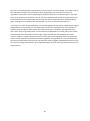
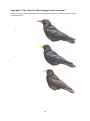
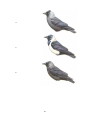
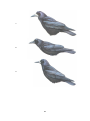
Appendix 3: The Dataset of Bird Images Used in Section 5 .................................................................. 56
1 Introduction
The functional significance of avian plumage colour and patterns has interested biologists for almost
150 years. There have been many hypotheses concerning this functional role: predator avoidance,
thermoregulation and social signalling, to name a few (Riegner, 2008). To test any of these
hypotheses you have to perform some kind of analysis on the plumage of the birds. Such an analysis
is of today rather subjective since the methods that are used still, to varying extent, rely on human
interpretations and decisions. Thus, the results of an analysis might not be the same if performed by
two individuals independently. Even though the results might not vary much it is still a problem and
removing as much of this uncertainty as possible is desired. Another problem that stems from this
subjective analysis is the difficulty of making quantitative measurements. When, for example,
analysing the colour of plumages it is very hard for a human to specify such quantities accurately.
Thus it is even harder to make comparisons that measure the similarity or dissimilarity in a set of
birds based on them. Such measurements would be very useful in understanding the functional role
of avian plumage colour and patterns. They would give a quantitative value that could then be
related to other statistical data like speciation rates, sexual selection and ecological data.
The purpose of this thesis work is therefore to develop a toolbox in MATLAB that will help biologists
to analyse the colour variation of birds in an objective way.
2 Objectives
The development of the toolbox can be divided into two sub goals:


The first is to find a way to represent bird plumages in a standardised digital image format
where bird images are warped into a specific template to allow for pixelwise comparison of
colours.
The second is to explore different ways to compare the bird plumages for the standardised
images. This involves statistical modelling of plumage variation ranging from simple pixelwise
calculations of mean and variance to more advanced methods such as principal component
analysis (PCA).
2.1 Limitations
It is not part of the thesis work to develop software that should be able to analyse an arbitrary set of
birds. The shape of birds can vary greatly over the different species and therefore it is enough if the
software can compare a set of birds with limited variation in shape.
Some restrictions on the nature of the bird images are allowed, e.g. that they should be from
approximately the same angle. Also, the focus can initially be on hand drawn illustrations since they
do not have as much noise in the relevant information. If time allows for it the software can be
extended to allow for photographs of birds.
3 Related research
Principal component analysis (PCA) on images is a well known technique. A famous paper by Turk
and Pentland (1991) describes how to use this technique as part of a face recognition system. First a
feature space that spans the most significant variations among a known set of faces were created by
4
representing each image as a vector and performing PCA on the set. These features are called
“eigenfaces” because they are the eigenvectors, or principal components, of the set of faces.
Individually they do not necessarily look like normal faces with distinct features such as eyes, noses
and ears. The best description would be that they look more like a ghostly illustration of a face.
However, each image in the set can be completely described by a weighted sum of these eigenfaces,
in other words a set of coordinates in the feature space they span. The projection operation could
then be used to characterise a new face image by a weighted sum of the eigenfaces. Therefore it was
possible to recognise a particular face by comparing these weights to those of known individuals. The
paper also brought forward algorithms to automatically learn to recognise new faces and also a way
to implement the face recognition in a near-real-time computer system.
4 Methods
The methods implemented to solve the task of this thesis work are described here, as well as some of
the theory behind them. The methods are ordered as they are thought to be used in an analysis.
4.1 MATLAB
The programming of all the code in this thesis work has been done in MATLAB (MathWorks). That
decision was made mainly because MATLAB allows for fast prototyping and has a large library of
useful tools including a set for image analysis.
MATLAB is an environment for numerical computing and visualisation of data developed by Math
Works and is available for the operating systems Windows, Mac OS X and Linux. It is a very flexible
environment commonly used in fields such as signal processing, image analysis, applied mathematics,
physics, biology, economics and anywhere numerical computing is useful. There are also many addon toolboxes available that can extend the MATLAB environment to specific applications. MATLAB
uses a high-level programming language and has many built-in functions which make it relatively fast
and easy to perform numerical calculations (MathWorks). Calculations are performed by either
writing individual commands in the command prompt or by chaining together commands in scripts.
You can also write your own functions and save them as m-files.
The name MATLAB comes from MATrix LABoratory and reflects the fact that the matrix is the basic
data type in MATLAB (Pärt-Enander & Sjöberg, 2003). This makes it very easy to handle matrices and
arrays of data and perform operations on them. Since images basically are matrices where each
element corresponds to a pixel it comes natural to use MATLAB for image analysis.
4.2 Acquiring Digital Images
The first step in image analysis is to acquire the actual images. In this case most of the interesting
ones will be found in different ornithological books as hand drawn illustrations. The advantage of
analysing hand drawn images is that the intraspecies variation in appearance can be taken out of the
equation. The purpose of the illustrations in the majority of ornithological books is to show the
characteristic traits of the different species not individual differences. Thus each illustration is more
or less an average representation of that species.
To perform computerised analysis on the images they first need to be digitised. This can be done in
three ways if the source is a printed book. The easiest way would be if a digital copy of the book was
5
available but that is almost never the case. The two more realistic options are to use either a digital
camera or a scanner, with the latter offering the most effortless process.
Using a camera is possible but it raises some issues that would have to be dealt with, such as
achieving uniform lightning and compensating for optical aberration. A uniform lightning of the
pages being photographed is needed for a correct colour reproduction of the actual images in the
book. If some part of the page is illuminated differently than any other part, the photo will get a
gradual difference in colour and/or brightness depending on the light sources. To eliminate this
problem the photo either has to be taken in ideal lightning conditions which requires a cumbersome
set up of light sources, or the variations in the image could be corrected afterwards which would also
require some work. Correcting for optical aberration also has to be done after the picture is taken
and it requires knowledge about the optics in the camera that was used. In short, using a camera to
acquire the images brings with it some additional work before the images are ready to be analysed.
A standard flatbed scanner on the other hand requires far less effort. It has its own illumination and
shielding against external light. The shielding is often not complete but enough to make external light
negligible. The scanner also eliminates the problem with optical aberration since it does not have any
significant optics. Since the scanner is much quicker and easier to use for image acquisition than a
digital camera, that is what has been used throughout this thesis work.
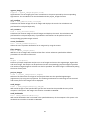
4.3 Halftone Problem
A problem that has to be dealt with when performing computerised analysis on images acquired
from books is the effect of halftone printing which is the technique most modern books are printed
with. To give some background, the technique was originally invented to make printing of grey levels
possible with the letterpress (Encyclopædia Britannica, 2011). The letterpress could only apply a
uniform layer of ink and the thickness could not be controlled. The result was the limitation of
printing either black or white and nothing in between. Halftone printing solved this problem by
breaking up the images into dots of ink with different size or spacing. By varying these parameters
the amount of ink applied to an area could be controlled, thus achieving different grey tones. The
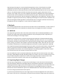
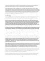
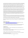
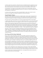
actual brightness of the dots is never changed but the trick lies in making use of the human eye’s
limited resolution. If the spacing and size of the dots are small enough a human viewing the print at
reading distance will not notice the individual dots in an area, instead the overall brightness will be
observed, Figure 4-1. If for example that area is covered to
by dots the visual grey tone is a
50/50 mix of black and white.
Figure 4-1 Left: Halftone dots. Right: How the human eye would perceive such a pattern from a distance far enough away.
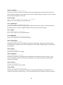
Halftone printing is not limited to grey tone images but it is also widely used to print in colour. The
basic principle is the same but there is more than one colour of ink to choose from. By breaking the
6
image up into one layer of dots for each ink and printing them one at a time the optical effect of a
full colour image can be achieved. The most common set of ink used for halftone printing today is
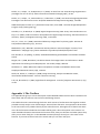
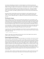
CMYK which stands for Cyan, Magenta, Yellow and Key (black), see Figure 4-2.
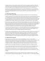
Figure 4-2 Three examples of colour halftoning using CMYK separations. From left to right: The cyan-, the magenta-, the
yellow- and the black separation followed by the combined halftone pattern and finally how the human eye would observe
the combined halftone pattern from a sufficient distance (http://en.wikipedia.org/wiki/File:Halftoningcolor.svg, retrieved
2011-10-26, with permission)
As mentioned before, analysing digital images that are acquired from halftone prints raises a
problem. Even though the halftone dots might trick the human eye, they are far more noticeable on
the pixel level which is where the analysis is done. The problem can be seen if the digital image is
zoomed in or a magnifying glass is used on the print. The dots form a kind of noise and will affect the
analysis of the digital image. The amount of noise will depend on a combination of the spacing of the
dots in the print and the resolution the image is scanned with. Decreasing the spacing of the dots
makes the print converge to a full continuous print which would not have any noise of this kind.
Scanning the print in a lower resolution would also lower the noise, since the dots would then be
averaged is some way, depending on the scanner hardware and software. However, the only part
that can be controlled is the resolution of the scan. Unfortunately there is no easy way of learning
what sort of averaging is done by the scanner when a resolution lower than the highest possible is
chosen. Because of this all prints were scanned in the rather high resolution of
dpi and were
later resized digitally. This allowed control of how the resolution was decreased.
4.4 Resizing
The main purpose of shrinking the images digitally is to control which method is used to shrink them.
As mentioned, the scanning was done in a rather high resolution to minimise the internal averaging
in the scanner. Representing the images in such a high resolution would be entirely pointless since it
is higher than the actual “information resolution” of the image. The interesting information is how
the bird looks not the position, size and colour of the halftone dots. Furthermore, unnecessarily high
resolution images would mean unnecessary high computation times. Therefore the images were
shrunk to a size that represents very little of this unnecessary information. So resizing is in other
words part of the reduction of the halftone related noise. All the noise is not expected to be removed
in this stage but it is the first of two steps that aim to achieve this. The final reduction is done with
standard Gaussian blur filtering which will be explained later.
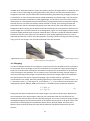
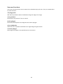
The other reason for resizing the images is to make them somewhat equal in size. If the set of birds
to be analysed contains birds of different scales then it is a good idea to shrink the larger ones down
to the scale of the rest of the images. The images will actually be made equal in size later anyway but
7
that final size is the average of the set, so if some of the birds differ much in scale from the rest the
average size will be noticeably affected. The result would be that the smaller images would be
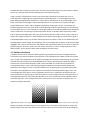
enlarged while the larger ones would be shrunk. The problem with this is that larger images usually
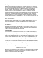
contain more details while smaller images usually have less detail. The enlarged smaller images
which contain less information will look blurred compared to the shrunk larger images, see Figure
4-3.
a
b
c
d
Figure 4-3 Comparison of images of different size being resized to the same size. a) Original large image. b) Original small
image. c) The large image after shrinking. d) The small image after enlarging.
This makes for a bad comparison since details on the larger image will be taken into account in the
analysis but the same detail on the smaller image will not be available or be distorted. This would
cause the analysis to make wrong conclusions concerning how alike the birds are and where they
differ. Therefore it is a good idea to resize some of the images individually if they differ much in scale.
It should be noted that the larger the set of birds is the less it will matter if a few birds are of a larger
scale since the final shape is just an average.
Lowering the resolution of the images was done with a built-in function in MATLAB called imresize.
The function has three different methods for performing the resizing of an image and the one that
was chosen was a method that uses bicubic convolution interpolation as described in the paper by
Keys (1981). For a reader unfamiliar with the concept of convolution, the basics can be found in most
of the fundamental books about image or signal processing like (Gonzalez & Woods, 2008) or
(Denbigh, 1998). Image resizing starts with the user selecting what ratio the image resolution should
resized with. The new image dimensions are then calculated as follows:
The ratio can have any value in the interval
. This creates a new raster of
pixels that now
has to be assigned brightness values. This is when the bicubic convolution interpolation comes into
8
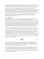
play. Simply put, the original image
is first overlaid on the newly calculated and empty raster
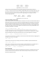
which is the image function we want to calculate, Figure 4-4.
Figure 4-4 The two overlaid pixel rasters. Thin lines: Original image raster. Thick lines: Newly calculated raster.
Since has more pixels than its raster will have to be compressed in order to fit, but to perform
the interpolation the two functions need to be expressed in the same coordinate system. The original
image is therefore described as a sampled function
, where and are integers, and
and
are the spacing between pixels in the coordinate system of . To view the problem straight
from an interpolation perspective – is the sampled data and is the continuous function that will
be interpolated from that data. It should be noted that a continuous function is not needed, the only
interesting points are the actual pixel coordinates of . However, the equations will still look the
same and the only difference will be that the values plugged into the equation of
will be
integers.
The brightness of
can be expressed by the convolution equation:
The function
is called the interpolation kernel and it is different for different types of
interpolation. Most common is that a relative small neighbourhood is used and pixels outside are set
to zero. Bicubic interpolation would use the nearest
neighbourhood of pixels in to calculate
the brightness of a pixel in .
Performing the interpolation in this way would mean that every pixel needs
multiplications and
additions to determine its brightness. It is actually not a large computational load but there is still
a simple way to reduce it to multiplications and additions. By using a so called separable
interpolation kernel the interpolation could instead be performed in one dimension at a time. A
separable kernel means that it, in our case, can be divided into two one dimensional kernels:
This turns Eq.
into
If the commutative and associative properties of the convolution is used then Eq.
rewritten as
9
can be
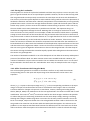
This means that by doing two convolutions with one dimensional kernels you can achieve the same
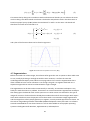
result as doing a two dimensional convolution. The bicubic interpolation used in this thesis work is
based on a paper by Keys (1981) where the two kernels and are the same. The kernel will
therefore from now on be referred to as:
and a plot of the function values can be found in Figure 4-5.
Figure 4-5 The bicubic interpolation kernel used,
.
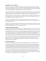
4.5 Segmentation
Before the actual scan of the images, the software often gives the user an option to select which area
to scan, usually by drawing a rectangle around the area. However, it is often the case that
ornithological books display several birds in one page. When this is true the segmentation that is
often available in basic scanner software is not enough. The goal is to segment each bird into a
separate image and that cannot be achieved with a single rectangle.
The segmentation can be done either automatically or manually. An automatic technique is very
handy if it works but there is a problem. There exists no universal automatic segmentation technique
that always gives the desired result. So the options are to either create one tailored for the type of
images of concern or find one that has already been made and works for these images. Both require
some work to be done. Since the purpose of this thesis work is not automatic image segmentation
and the images have a fairly simple geometry to segment, a mostly manual approach was chosen. For
this task an image editing software called GIMP (GIMP Development Team) was used. It is software
external to MATLAB but it was chosen because it is free and available to most popular operating
systems including Microsoft Windows, Apple Mac OS X, and GNU/Linux.
10
In GIMP a tool called Free Selection (Lasso) was used to perform the segmentation. It allows the user
to select an area of the image by tracing a boundary. The selection can then be inverted and the
background removed. The tool allows both free-hand drawing and positioning of polygon vertices or
a combination. It also has two useful options called Antialiasing and Feather Edges. The first simply
smoothes the boundary somewhat to avoid jagged edges. The second is even more useful since it
allows pixels on a desired distance from the boundary to be gradually selected. The pixels inside the
selection that are not within the distance will be selected as normal. Then moving outwards the
pixels will be less and less selected meaning that more and more of their value will be left in the
background. When reaching the set distance outside the boundary no more pixels are selected. The
result is edges with a smooth transition to the background, Figure 4-6. So the edges will look as they
have been slightly blurred which is actually a desired effect, why this is preferred will be described in
the Section 4.8. This softer type of cut also allows for faster image segmentation since it is not as
important to follow the contour of the bird precisely. Choosing a distance setting was done by simply
trying it out on one image in the set until the desired effect was achieved.
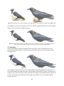
Figure 4-6 Segmentation of image done using feathering in GIMP. Left: Original image. Right: Segmented image, note the
gradual transition to the background.
4.6 Warping
In order to compare the birds in the images on a pixel per pixel level, the pixels need to correspond
to one another across all images. A pixel on one bird has to correspond to a pixel representing the
same part of another bird, meaning the coordinate of a specific part of the bird has to be the same
across all images to be compared. This is certainly not the case with the newly scanned images so
some pre-processing of the images is required. More precisely the images need to be warped into
the same shape so they can be compared. Warping is just another word for a geometric
transformation of an image. Generally speaking a geometric transformation is a vector function, say
, that takes a pixel
and maps it to a new postion
, this is done for all the pixels in the
image (Sonka, Hlavac, & Boyle, 2008). The function is divided into two component equations
Getting the new pixel coordinates for the output image is only the first of two steps. Whereas the
pixel coordinates of the input image are discrete, the coordinates after the transformation are
continuous and will most likely not fit the discrete pixel grid. So in order to make the output image a
valid digital image the discrete pixel positions of the desired output grid has to be given values. This
second step is called brightness interpolation (Sonka, Hlavac, & Boyle, 2008). There are many
different ways to perform these two steps and the methods used will be described in the next
sections.
11
The warping procedure used for the different methods in this thesis work differs somewhat from the
general case recently described. Instead of calculating the transformation functions that transforms
the pixels in the input image to their position in the output image, the inverse transformation is
calculated. In other words the sought transformation function is the one that calculates the
corresponding position in the input image for all the output pixels. So
in Eq.
represents the
pixels in the output image and
represents their corresponding coordinate in the input image.
This means that the brightness interpolation also will differ a bit. Assigning values to the output
pixels is done by interpolating in the domain of the input image. The pixels of the input image are the
known data points and the values of the output pixels are found by interpolating the values
(brightness) at the coordinates
. These interpolated values are then assigned to the
corresponding pixel in the output image.
4.6.1 Landmarks
The transformation functions and are sometimes known in advance but if they are not, as in
the case of this thesis work, they have to be determined before the actual warping can be
performed. To determine them a number of corresponding pixel coordinates, points, in the input and
output image are needed. The number of point pairs needed depends on the method being used and
in general more advanced methods require more known pairs. The problem is that the points in the
output image are not known. The solution is to use landmarks. They are user selected points that the
transformation algorithm can use to determine and . In other words the user helps the
algorithm by identifying some points in the input and output image that correspond to each other.
In this case the procedure will be slightly different though. The goal will be to get all the birds in the
image set into the same shape but this shape still has to be determined somehow. A fairly simple but
intuitive approach was chosen for this. All the birds were transformed into the mean shape of the
set. To get the mean shape the user first has to position landmarks on all the images in the set. As
mentioned the landmarks have to be placed in the same way on all the images. Denote the
landmarks
where
,
, is the number of landmarks placed on each image and
is the number of images in the set. That means has to be placed on the same anatomical part of
the bird across all images. When that has been done the mean shape of the birds is calculated by
taking the mean of the landmarks
where
is the :th landmark in the mean shape. Now that a set of corresponding points is known,
the transformation functions can be determined. Each image will have its own transformation
functions, for the :th image they will be
and . How these functions are determined depends
on the method used and will be described in the next sections.
In order to make sure the whole image is warped and no area is mistakenly left out four landmarks
were automatically added to the user selected ones. One in each corner of the image. This also
means that the dimensions of output image is automatically calculated when the mean shape is
calculated. All the warped images will have the same dimensions which will be equal to the mean of
the dimensions of the input images.
12
4.6.2 Placing the Landmarks
Choosing where on the birds to place the landmarks and how many to place is not an easy task. The
goal is to get all the birds into an as equal shape as possible. However, the fact is that the only pixels
that are guaranteed to end up exactly as wanted in the new shape are the ones with landmarks on.
The accuracy of the other pixels depends on what method is being used but also on the placement of
landmarks. Geometric transformation is basically interpolation so more landmarks per area generally
produce better result. It lowers the average distance between a pixel and the known points and the
further away a pixel is, the less accurate the method is in determining its position. That is not to say
the user should cram as many landmarks as possible onto the birds. The important thing is to
landmark the irregularities amongst the birds. Meaning that it is enough to mark where an area
starts and ends if it is fairly uniform. As an example, consider the breast of a bird: Here it is probably
enough to mark the borders of the breast like the wing and actual end of the bird since the breast is
fairly uniform with no distinct anatomical features in it. It might therefore be ok for it to be stretched
or compressed based only on the landmarks that define its border. However, if there were some
feature of interest on the breast that should be compared across the birds then that would have to
be landmarked. So for best results the landmarks should be placed on important features of the bird
and where there are irregularities. When it comes to the contour of the bird it is important to mark
that out since it gives the algorithm information on where in the image the bird is and the shape of
the contour. Placing the landmarks somewhat equally spaced and marking distinct discontinuities in
the contour is a good approach.
The number of landmarks needed for a set of birds depends on how alike the anatomy and depicted
posture of the different birds are. More variation means more needed landmarks. However, the
number of landmarks only has to be increased in the area where the variation occurs. For the set of
birds examined in this thesis work 30 – 40 landmarks were used, an example can be seen in Figure
5-3.
4.6.3 Affine Transform with Triangular Mesh
One of the simplest geometric transforms is the affine transform. It only needs three known
corresponding points in the input and output image to be determined as can be seen in the
equations
where
is a point in the output image and
is the corresponding coordinate in the input
image. A new pair of transformation functions is calculated for each image in the set. The affine
transform allows for changes in shape such as translation, rotation, skewing and scaling (Sonka,
Hlavac, & Boyle, 2008). This method was the first one approached in this thesis work but with a small
modification. If the same
and
would to be used for the whole image it would not be possible
to achieve the goal of transforming all the birds into the same shape. Simply rotating, translating,
skewing and scaling the whole image does not account for the many internal variations across the
birds. For example, maybe one feather has to be enlarged while another needs to be shrunk or the
wing needs to be rotated in one direction while the beak needs the opposite. The solution to this
problem is to use separate transformation functions for different parts of a bird. Each one of these
affine transforms needs three points to be determined. Therefore it is natural to divide the image
13
into areas spanned by three points, in other words triangles. With the landmarks as these points a
triangular mesh is calculated using Delaunay triangulation, invented by Boris Delaunay in his paper
(1934).
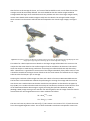
The triangulation of a set of points is a set of connected straight lines whose vertices are the points
being triangulated. The lines do not intersect each other except at the vertices and every region
bounded by a set of these lines is a triangle. Finally, the outermost lines of the triangulation form a
convex hull (Lee & Lin, 1986). This means that a straight line drawn between any two of the points in
the convex hull will lie entirely within or on the hull (Gonzalez & Woods, 2008). The Delaunay
triangulation is a triangulation that also fulfils the property that the circle which passes through the
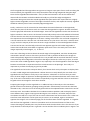
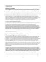
vertices of any triangle will not have any other points in its interior, Figure 4-7.
Figure 4-7 Delaunay triangulation of 8 points with the circles that passes through the vertices of the triangles drawn out.
With the image separated into multiple areas different parts of the birds can be reshaped individually
making it possible to account for varying types of differences in the birds. The transformation
functions, Eq.
, for each triangle in each image can now be calculated using the corresponding
landmark coordinates in the images and in the mean shape. When all the transformation functions
have been determined the images can be transformed into the mean shape. To clarify, the pixels
within a triangle will be transformed using the transformation function for that triangle.
4.6.4 The Function griddata
A built-in function in MATLAB, called griddata, was used to implement affine transformation with a
triangular mesh as well as another more advanced geometric transformation that uses biharmonic
splines. The function is actually an interpolation function that works for non-uniformly spaced data
but it can be used for geometric transformation as well. Consider Eq.
, it consists of two dimensional functions that takes an - and -value and returns the new - or -coordinate as its
function value. They are separate equations so one can be determined without knowing the other.
The functions can therefore be viewed as two separate interpolation problems where the data points
and their value, or , are known and are therefore described by
14
where
and are the number of landmarks, and
where are the number of
images. Determining the functions is therefore a matter of interpolating the function values at the
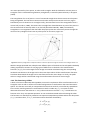
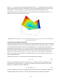
intermediate - and -coordinates, for an illustration see Figure 4-8. If the figure were a
representation of one of the functions in Eq.
, then the -axis would represent either or
and the - and -axis would represent and .
Figure 4-8 Surface interpolated from the non-uniformly spaced points
linear affine transformation.
shown as black dots, using griddata with
4.6.5 Biharmonic Spline Interpolation
A powerful method made easily available by the function griddata is biharmonic spline interpolation.
It finds the biharmonic function
that passes through the known data points, where is a point
in a -dimensional space which in this case is described by
. As mentioned, two separate
interpolations have to be done,
and
but since the only difference between them will be
the data they handle the general case will be described. Do not be confused by the notation , it
represents the same type of function as in Eq.
but since it in this case will be a biharmonic
function the notation will be used. The complete derivation of this method can be found in the
paper by Sandwell (1987).
A biharmonic function, , is a function that solves the biharmonic equation
where
is the biharmonic operator. The surface
is made up of a linear combination of so
called biharmonic Green functions , , which are centred at each known data point. The Green
function for -dimensional space is defined as
In order to make the functions pass through the known data points their amplitude is adjusted by
multiplying them with a constant . Now the actual equations that needs to be solved are
15
where is the Dirac delta function,
general solution to this equation is
The values of
are the known data points and
are the number of them. The
are found by solving the linear system
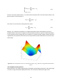
With Eq.
solved the interpolation is complete. Biharmonic spline interpolation, Figure 4-9,
produces better results than a triangular mesh based affine transform, Figure 4-8. Most noticeably it
is a lot smoother and an analogy that can be made is to consider the input image a rubber sheet that
is grabbed by the landmarks and stretched and compressed until the landmarks fit over those in the
mean shape.
Figure 4-9 Surface interpolated from the non-uniformly spaced points
splines.
, black dots, using griddata with biharmonic
4.6.6 Brightness Interpolation
With each pixel in the output image having a calculated corresponding coordinate in the input image
it is time to assign those pixels appropriate values. The situation is illustrated in Figure 4-10.
16
Figure 4-10 The calculated corresponding coordinates (red dots) of the pixels in the output image, here seen in the domain
of the input image. In this case the input image has
pixels and the output image .
The interpolation is performed in the domain of the input image by using the coordinates and values
of the pixels in the input image as the known data points. The sought pixel values of the output grid
are then interpolated using the coordinates obtained from the geometric transformation. The
interpolated values are then assigned to the corresponding pixel in the output image. The problem is
very similar to the interpolation problem described in Section 4.4 and the same method of bicubic
convolution interpolation (Keys, 1981) can be used. Meaning that the convolution equation, Eq.
,
and the separable interpolation kernel, Eq.
, can be used to perform the brightness interpolation
as well.
MATLAB has a built-in function that handles interpolation of two-dimensional functions where the
known data points are uniformly spaced, which fits our case perfectly. The function is called interp2
and it has a few different methods of interpolation including bicubic convolution. The result of an
interpolation done in the fictional situation of Figure 4-10 using interp2 can be seen in Figure 4-11.
Figure 4-11 Pixel values of the input image (surface) with the interpolated pixel values of the output image (black crosses).
Interpolation done with the function interp2 using bicubic convolution.
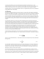
4.7 Removing Unwanted Variance
When the warping of the bird images is done the result can be evaluated to some degree by looking
at the variance image of the warped set of images. This makes it especially easy to detect how the
17
warping performed at the contour of the birds. Contour misalignment will show quite clearly as it
results in high variance as can be seen in Figure 4-12.
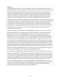
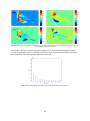
Figure 4-12 Variance image of the tail feathers calculated from a set of warped birds. A higher variance shows as a warmer
colour.
It is also possible to detect if the interior features were warped correctly by looking for variance
patterns that should not be there. If this is the case and the misalignment is serious enough, the
warping procedure should be done over with another set of landmarks. Having high variance in
places it should not be in will result in a reduced quality of the coming analysis which will be
explained later. The toolbox has no way to know if the variance of the warped image set is due to
misalignment or actual variance in plumage colour. However, if the only problem is the contour then
it could be fixed without redoing the warping.
The variance of any part of the warped images can be removed by setting the corresponding pixels to
the same value across all the images. A pixel with the same value in all the images has zero variance.
Setting the corresponding pixels is easy since they have the same coordinates in all the warped
images (that was the whole idea with the warping). So if the user selects the pixels in the variance
image that are the variance he wants to remove, it is only a matter of setting the pixels at those
coordinates to the same value in all the warped images. The actual pixel value they should be set to
was chosen as the background colour (white) since that is the colour the contour borders to. It is
important to note that this procedure will alter the warped images. Visually it will look as though
parts of the contour have been cut away. However, as long as the information at the very outline of
the bird is not considered very important this is a viable option to spending time trying to get a near
perfect warping of the images. There is actually no point in analysing a set of warped images that
suffer from some misalignment without first removing the unwanted variance at the contour. No
valuable information can be gathered from those parts of the contour anyway since the
correspondence between pixels is not correct.
To make it easier for the user to select pixels in the variance image the selection is done by
surrounding the desired area with a polygon. The user positions the vertices of the polygon and
when it is closed all the pixels that lie inside it are selected, Figure 4-13. To decide which pixels lie
inside the polygon the point-in-polygon algorithm described in the paper (Alciatore & Miranda, 1995)
is used. It is an algorithm based on winding numbers. What it basically does is measuring the number
of times a polygon winds around each point and from that information it determines if the point is
inside or not.
18
Figure 4-13 Left: Area of variance image selected by positioning polygon vertices using the toolbox. Right: Area removed.
4.7.1 Studying Specific Regions of the Birds
The same methods can be used to select specific regions of the birds for analysis. In other words, to
cut away everything except a desired region from the warped bird images. The advantage of this
would be that the coming analysis methods will not have to take the whole birds into account but
can instead focus on the desired region. As will be described later on, the PCA algorithm looks at the
whole variance of the images in the set. If the user is only interested in a certain region of the birds
then all the other variance will be uninteresting but the algorithm will still use all the variance. If the
region is isolated prior to the PCA the algorithm can focus on how that area varies without also
having to describe the rest of the bird in the same image. For example: a region that could be
described to
with four eigenvectors, if analysed separately, could, if analysed as part of the
whole bird, need a lot more eigenvectors (eigenbirds) to be described to the same degree. An
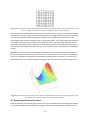
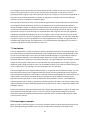
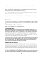
example can be seen in Figure 4-14.
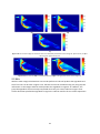
Figure 4-14 Top: Mean image of a set of warped birds and the respective cumulative sum of the variance represented by
the four first eigenvectors. Bottom: Mean image of the chest area of the same bird set and the respective cumulative sum
of the variance represented by the four first eigenvectors.
19
It is much more efficient to cut out a specific region of the bird in this phase than it is in the
segmentation phase. Here the same cut is done in all the images at the same time meaning the user
only has to select the area once. This works because the images have been aligned during the
warping procedure. If the same thing would be done in the segmentation phase the user would have
to do a separate cut in every image.
4.8 Filtering
Filtering of the images was done for two main reasons: to reduce the noise caused by the halftone
dots, and to blur edges in the images. To counteract the noise it first has to be analysed. As explained
before it is a product of the halftone printing procedure which means the image is made up of tiny
multi-coloured dots that give the optical illusion of a continuous full colour image. Performing some
kind of averaging on the image would basically smear all the dots so they merge with each other and
the background, creating a more seamless version of the image, which seems to be exactly what is
needed.
As mentioned in Section 4.4, the first part of the total filtering process was done by resizing the
images using bicubic convolution interpolation. This means that the resized images will already have
lost some of the problematic half tone characteristics but they still need more filtering done on
them. With the resizing already having merged some of the neighbouring pixels, it was assumed that
the pixels in the resized image were more representative of the actual pixel value at their own
coordinate than at the neighbouring coordinates. However, it was also assumed that some
information of the pixel value at a given coordinate will still be located at the neighbouring pixels.
Therefore a type of local averaging filter that prioritises pixels based on their closeness to the centre
was chosen, more specifically a Gaussian filter.
Gaussian filtering is basically done in the same manner as the bicubic convolution interpolation in
Section 4.4 but with two differences. First, a Gaussian kernel is used which in -dimension is defined
by
where is the standard deviation,
factor given by
is the distance from the current pixel and
is the normalisation
is the number of pixels in the kernel and is the value of the kernel at . The other difference is
that the pixels, in the output image, whose values are being calculated lie at the same positions as
the pixel in the input image. The Gaussian kernel is also separable so the filtering can be done one
dimension at a time in the same way as before.
There are two parameters to tune in a Gaussian filter; the standard deviation and the size of the
kernel. The standard deviation basically decides how wide the Gaussian shape should be. The size of
the kernel is the size in pixels the kernel should have when performing the convolution. Choosing the
right parameters for the filter is not trivial. It is often possible to make a somewhat accurate guess
20
based on the nature of the images and the noise but after that fine-tuning by trial and error will most
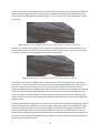
likely be the best approach. In this case the noise is caused by the halftone printing process which
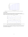
creates patterns of the CMYK-coloured dots, Figure 4-15. As can be seen, there is definitely a pattern
to the noise.
Figure 4-15 Image scanned in
dpi. Note the almost circular pattern caused by the half tone dots.
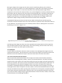
However, the images to be filtered are the resized ones which have already had some of the noise
removed but there is still a pattern to the remaining noise, see Figure 4-16. In this case it is possible
to make out a kind of reoccurring grid shaped pattern in the image.
Figure 4-16 Resized image. Note that the image has been zoomed for easier comparison.
These observations are very helpful since it makes it easier to choose the parameters of the filter.
Since there is a reoccurring pattern in the noise it was considered a good idea to start with a kernel
size that is approximately as many pixels as the interval of the pattern. The existence of such a
pattern was believed to be caused by some inherent pattern in the halftone printing process and that
information about a pixel could be spread out in at least one interval. Therefore averaging over an
area of the same size was thought to only take into account the information of one iteration of the
pattern. However, this was just an initial guess and some small adjustments in size were made to get
the best results.
Deciding what standard deviation to use was more of a trial and error procedure. Depending on what
kernel size was chosen, a guideline is to choose sigma at least high enough so the whole kernel gets
somewhat significant values. If the values at the edges at the kernel are negligible compared to the
centre values it might be better to decrease the kernel size. A limit in the other direction is to not
choose sigma so high that the kernel basically becomes a standard average filter where all values are
the same. The centre pixel should hold the most relevant information after the resizing procedure so
the kernel should emphasise that.
21
Blurring the edges of the images was the other reason for performing filtering. This is desired
because it increases the tolerance for small misalignments in shape due to the warping procedure.
Sharp edges at the borders or in the internal structure of the bird will produce large variance
component in the result of the analysis if there is any such misalignment. Variance produced this way
will interfere with the analysis of the actual colour of the plumage and it is therefore undesired. By
filtering the images with a blurring filter the edges are smoothed and thus go from being a sharp
change in pixel intensity to a more gradual change. This smearing out of the edges makes it less
important for edges to align perfectly and small errors becomes more manageable.
In MATLAB the filtering was done with the function imfilter which performs the filtering using
correlation instead of convolution but in this case the kernel is symmetric which means there will not
be any difference. The actual kernel is first created by another function called fspecial. The result of
the filtering can be seen in Figure 4-17.
Figure 4-17 Image filtered using a Gaussian blur filter with kernel size
and
zoomed for easier comparison.
. Note that the image has been
The filtering of the images was done as the last step before the analysis because of the simple fact
that information about the input image always is lost in blur-filtering. And since there was not any
reason to do it before any other stage, it was done here.
4.9 Analysis
In order to get any information about the colour variations in the plumages the images have to be
analysed in some manner. The data we want to extract from the images are of statistical nature and
therefore most of the methods of analysis used in this thesis work are of that same nature.
4.9.1 Basic Statistical Measurements
Some easy but still useful measurements of the images can be done with some basic statistical
analysis such as calculating mean, median, variance and standard deviation. The birds have been
warped into the same shape so the same pixel coordinate across the image set should represent the
same part of the bird. The accuracy of this correspondence between pixels and parts of the bird is of
course dependent on how well the warping was done. In any case, this means that if each pixel
coordinate is considered separately and all the values of that pixel across the image set are taken, a
meaningful subset of data is acquired. The mean, median, variance and standard deviation can then
easily be calculated on that subset. By doing these calculations for all the pixels a complete image for
each of these statistical attributes will be achieved. Due to the correspondence between pixels and
parts of the bird these images will give a good measurement of what the mean, median, variance and
standard deviation of the plumages would be.
22
4.9.2 PCA
Principal component analysis is a linear transform that, given a set of data that is represented as
multidimensional vectors, will determine the orthogonal coordinate system that has its basis vectors
follow the modes of greatest variation in that data. The new basis vectors are called principal
components and will be as many as the dimensionality of the dataset. The first component will
represent as much of the variance in the data as possible, and each succeeding component will
represent as much of the remaining variance as possible. It should be noted that the principal
components are not statistical variance measurements in themselves, they only describe the
variation in the data. The principal components are the eigenvectors of the covariance matrix of the
dataset where the eigenvector with the largest eigenvalue is the first principal component and so on
(Turk & Pentland, 1991). Since the new coordinate system is orthogonal, the data will always be
uncorrelated when it is represented in this way regardless of its original state (Sonka, Hlavac, &
Boyle, 2008). PCA can also be used for dimensionality reduction by choosing to represent the data
with only some of the first principal components. The data will retain the characteristics that
contribute most to its variance.
It might not be clear right away how PCA would be applied to images since they are not vectors.
Converting them to vectors is actually really easy. When the images in the set all have the same
dimensions,
if the images have three colour channels, they can just as well be
represented as vectors where each pixel value is a coordinate in a separate dimension. So every
image becomes a vector of length
, or expressed differently a point in a space with as
many dimensions. Performing PCA on the image vectors will give the eigenvectors of the set and
since these will have the same dimensionality as the data they can also be represented as images.
The eigenvectors are in fact linear combinations of the original images and will therefore share the
basic visual appearance of the original data (Turk & Pentland, 1991). The images dealt with in this
thesis work are of birds and therefore the eigenvectors (principal components) will from now on be
referred to as eigenbirds. The calculated eigenbirds can be seen as a set of features that together
describe the variation between bird images. They span a feature space and each bird in the dataset
will be exactly described by a point in this space (Turk & Pentland, 1991).
The reason PCA was considered an appropriate method of analysis for this thesis work was that it
would show how different parts of the birds vary together. An eigenbird describes as much of the
variation in the dataset as possible that has not already been described by an earlier eigenbird. This
means that the first eigenbird would show us what parts of the birds that describe the most of the
variation, the second what parts that describe the second most and so on. This information should
not be confused with the variance of the image set that was explained in the previous section.
Variance and standard deviation calculations work explicitly on the pixel level with no regard to any
other pixel than the one being calculated. The eigenbirds on the other hand describe the overall
variation of the image set. An example can be seen in Figure 4-18 which shows the standard
deviation and the first eigenbird of the image set in Appendix 3.
23
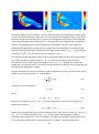
Figure 4-18 Standard deviation (left) versus the first eigenbird (right). Images are colour coded according to their respective
colour bar.
Studying the edges in the two images, it can be seen that the warping misalignment comes through
clearly in the standard deviation figure but is far less prominent in the eigenbird figure, especially in
the lower part of the tail feathers. This is because the misalignment in some parts of the edges did
not contribute enough of the overall variance in the image set to be included in the first eigenbird.
However, the misalignments are sure to be described somewhere in the rest of the eigenbirds.
Calculating the eigenbirds is actually not that complicated and the procedure can be found in the
paper by Turk & Pentland (1991). Denote the bird image vectors in the set
and the mean
of the set
, are column vectors of length
.
First the mean needs to be subtracted from all the images. This gives a set of vectors that describes
how each image differs from the mean
. These are the vectors that PCA will be
performed on and the result will be orthogonal vectors ,
which are the principal
components. So the eigenvectors are in fact the eigenbirds but to represent them visually they will
first need to be reshaped into images.
As mentioned before the principal components are the eigenvectors of the covariance matrix of the
dataset. The observed covariance, , is calculated by
which also can be calculated by
where
Meaning is a matrix of size
therefore be written as
. The eigenvectors of the covariance matrix can
where
are the eigenvalues. This is where a problem occurs. The matrix is of size
and determining all the
eigenvectors and eigenvalues would be
computationally cumbersome. To give an example: An image set of relatively small dimensions, say
pixels, would have a covariance matrix of size
which means
24
approximately
elements. Storing all these elements would also take up a lot of memory
since every element would need 64 bits (double precision). This means a total of
would be needed to store the covariance matrix alone. It would also be
unnecessary to perform these calculations if the number of datapoints are less than the dimensions
of the space
. Because then there would only be
meaningful eigenvectors
anyway and the remaining ones would have eigenvalues equal zero (Turk & Pentland, 1991).
The solution is to calculate the eigenvectors of an
matrix instead and then use these to form
the wanted eigenvectors, , by making appropriate linear combinations of the image vectors. This is
done by first studying the eigenvector calculations of the
matrix
where
are the eigenvalues and
are the eigenvector. Premultiplying both sides with
gives
Comparing this with Eq.
it can be seen that
are actually the eigenvectors, , of
.
This also means that the eigenvalues are the same as . So instead of directly calculating the
eigenvectors of the very large matrix , a slight detour is taken that reduces the computational load
and memory requirements. Using this insight the
matrix
is constructed and used to
first calculate . The elements of will have the property
. The eigenvectors of
are the vectors that fulfill
When they have been found they are used to determine the linear combination of the
vectors in the dataset that will form the sought after eigenbirds .
where
is the :th element of vector
matrix multiplications
. Calculating Eq.
image
is the same as performing the simple
These are the eigenbirds, their associated eigenvalues will alow us to rank them according to their
usefulness in describing the variation in the image dataset.
A note should be made about the way the eigenbirds actually are calculated in MATLAB. The
algorithm is an iterative one and to start it MATLAB makes a random initial guess. Because of this the
signs of the calculated eigenbirds can change every time the calculations are performed, even if input
is exactly the same. In other words this could very well be true for the first eigenbird of the image
dataset.
25
where would be the eigenbird calculated the first time and
the one calculated another time.
This is actually not a big problem since the only difference is in how the images in the dataset are
described in terms of a linear combination of eigenbirds. The coordinate that represents the
eigenbird in Eq.
will be negative in one case and positive in the other but the magnitude will be
the same. As long as the same set of eigenbirds is used throughout the analysis process this will not
cause any trouble.
4.9.3 Analysing the Eigenbirds
The eigenbirds can be analysed in multiple ways. The first and perhaps easiest way is to simply
display them as images and study them with your eyes. Eigenvectors are, however, not natural
images so they have to first be manipulated to fit the image format. This includes reshaping them
from vectors to three channel (RGB colour) image matrices but also scaling the coordinates to
acceptable pixel values. The resulting images will provide a general idea of the variations in the
image set but they can be deceptive. Eigenvectors have signed values whereas the unsigned 8-bit
pixel values are in the interval
. The reason why the values are signed is simply because they
describe the variation from the mean and this can be both positive and negative. The global negative
extreme value of an eigenbird will therefore be mapped to zero in the displayed image and the real
zero of the eigenbird will end up somewhere in the middle of and
. For greyscale images the
colour representing zero variation would be some intermediate grey tone, darker tones would mean
larger negative variations and brighter tones larger positive variations. There is also another problem,
the calculated eigenbirds of an image set will not have the same range of values which means the
grey tone representing zero will not be the same across the eigenbirds. All this goes against how we
intuitively perceive an image and it is therefore important to keep these things in mind when
studying the eigenbirds displayed in this manner.
A better way to display the information in the eigenbirds is to colour code the information using a
colour palette arranged after temperature, or more correctly wavelength, and a reference bar
between colour and values next to the image. It becomes a lot easier to interpret them as can be
seen in Figure 4-19.
Figure 4-19 Greyscale representation (left) versus colour coded representation (right) of a single-colour-channel eigenbird.
Note that there is now way to tell where the zero-level is in the greyscale version.
There is, however, a limitation to this colour coding. It only works for one channel at a time so each
eigenbird will be represented by a number of colour coded images equal to the number of colour
channels in the eigenbirds. An eigenbird in RGB would therefore have to be represented by three
separate colour coded images.
The calculation of the eigenbirds is based on the variation found in the images being analysed. It is
therefore important that the existing variance in the warped set of images actually represents the
26
variation to be analysed. Unremoved background elements or misalignment in the birds due to
unsatisfactory warping will create false variation that to the PCA algorithm will look exactly as the
real variation in the plumage colour. The calculated eigenbirds will therefore try to describe this false
variation as well and loose some of the focus on the real variation which means the result of the
analysis will be affected negatively.
4.9.4 Projection and Approximation
Studying the eigenbirds by eye is not the only way to analyse them. As mentioned before the
eigenbirds are a linear combination of the mean subtracted images in the dataset which means that
the images are also a linear combination of eigenbirds. Each image can be completely described by
an -dimensional coordinate together with the mean image . It can be interesting to look at these
coordinates since they say how much of each eigenbird the birds in the set consist of. Even more
interesting is to see how well the different birds are represented using only some of the first
eigenbirds. In other words approximating the birds in the set with a number of eigenbirds
.
Because of the way PCA works the first few eigenbirds should describe the overall features of each
bird quite reasonably, assuming that the birds were somewhat similar, and adding more eigenbirds
to their description should bring out more and more individual features.
In order to actually do anything like this the coordinates of each image has to be determined.
Calculating them is not at all complicated it is just a simple matter of vector projection. As mentioned
before the eigenbirds are eigenvectors that span a kind of feature space and each image in the
dataset can be represented by point in this space. To get the coordinates of these points each meansubtracted image has to be projected onto each of the eigenbirds in turn. Projection can be thought
of as calculating the ‘shadow’ one vector casts on another, Figure 4-20.
Figure 4-20 2-D vector projection. Vector
is projected onto vector
The resulting vector, , of projecting the image
where
is the length of vector
and
thus resulting in vector .
onto the eigenbird
can be calculated with
is the unit vector in the direction of
. But in this case the
only thing of interest is the length of in relation to the length of since this will be the amount of
the eigenbird that contributes to the description of . The length of can be calculated with the
dot product
and thus the length of
in relation to the length of
27
is
So this is what has to be calculated for each image and each eigenbird in order to find how much of
each eigenbird the images consist of.
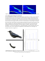
Apart from approximating the images with some of the first eigenbirds there is another easy analysis
that can be made. By studying the coordinates of the images in the space spanned by the eigenbirds
cluster patterns can be found. Birds that are relatively close to one another in this space should also
have similar plumage colour and vice versa. A quick way to get a basic overview of the clustering is to
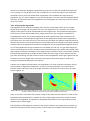
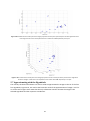
plot the image points in the space spanned by the first two or three eigenbirds since this will give a or -dimensional scatter plot where it is easy to see if there is any distinct clustering, Figure 4-21. As
mentioned before the first eigenbirds describe the most of the variance in the set so a scatter plot of
the first three could actually be quite informative. However, examining clustering was not part of the
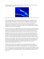
thesis work so there has not been much effort put into this.
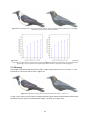
Figure 4-21 Image set of
birds projected onto the plane spanned by the second and third eigenvector.
5 Results
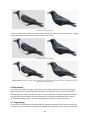
In this section the results that can be attained when using the toolbox on a set of bird images will be
shown. The image set used can be found in Appendix 3 but all birds will not be shown after each step
since that would take up too much space. Instead two chosen birds from this set will be used to show
the results of each step, they will be referred to as Image 1 and 2.
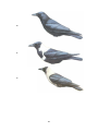
5.1 Segmenting and Resizing
The order of in which segmentation and resizing is done is not important unless some birds need
different resize ratios. In this case the scanned pages from the books were first roughly segmented
into individual images with one bird in each, see Figure 5-1.
28
Figure 5-1 Images segmented roughly using GIMP. They were segmented from a 600 dpi scan. Left: Image . Right: Image
.
The images were then all resized with a ratio of
using the feathering option in GIMP, Figure 5-2.
and then segmented again but more thoroughly
Figure 5-2 The final segmentation of the birds after they were resized with a ration of 0.3. The background, legs and
feathers from the other side has been cut away with the feathering option in GIMP enabled.
5.2 Warping
Now the bird images need to be warped into the same shape. To do that landmarks has to be
positioned on all birds and for this experiment
landmarks, Figure 5-3, were considered to give
satisfying results.
Figure 5-3 Bird images with
landmarks positioned.
The warping can be done with any of the methods allowed by the MATLAB function griddata. The
result from warping the images with affine transformation and biharmonic splines can both be seen
in Figure 5-4. For the continuation of the experiment the images warped with biharmonic splines will
be used. The landmarks that define the mean shape can be drawn out on the warped images if
desired, Figure 5-5.
29
Figure 5-4 Top: Bird images warped into the same shape using affine linear transform. Bottom: Bird images warped into the
same shape using biharmonic splines. Note that Image and now have the same shape and size.
Figure 5-5 Bird images warped using biharmonic splines with the landmarks of the mean shape shown on them. Note the
four automatically added landmarks in the corners of the image.
Taking a quick look at the variance image of the image set, Figure 5-6, it can be seen that there is
some misalignment at the edges of the left image. One way to cope with it is to use the function
remove_variance. Removing variance until the image looks like the right image in Figure 5-6 would
further segment the warped images as can be seen in Figure 5-7. Unless otherwise specified these
further segmented images are the ones that will be used for the rest of the experiment. An example
of how removing some of the variance affects the results of the analysis can be seen in Figure 5-8.
Figure 5-6 Left: Variance image of the warped set. Right: Variance image of the warped set after the use of the function
remove_variance. Note that the left image contains higher variance values than the right.
30
Figure 5-7 Warped images after the use of the function remove_variance. Note the further segmentation of the edges,
especially at the lower part and the tail feathers.
Figure 5-8 Comparison of the cumulative sum of the variation represented by the six first eigenbirds. Left: PCA performed
on the image set represented by the left image in Figure 5-6. Right: PCA performed on the image set represented by the
right image in Figure 5-6. Note that a higher degree of the variation is represented in the right figure.
5.3 Filtering
The images were filtered with the function filter_images using a kernel size of
the Gaussian. The results can be seen in Figure 5-9.
Figure 5-9 Images filtered using a Gaussian blur filter with kernel size
and
and
for
.
To give a more clear view of how the resizing and filtering have dealt with the halftone related noise
the effect of these steps on the bird head in image can be seen in Figure 5-10.
31
b)
a)
c)
Figure 5-10 Close ups of the bird head in image . Note the effect on the halftone dots. a) Image acquired from a
scan. b) Image after resizing with a ratio of
. c) Image after filtering with a kernel size of
and
.
dpi
5.4 Basic Statistical Measurements
To perform the principal component analysis on the filtered images the mean of the image set first
has to be calculated. It is also possible to calculate the median image although it is not needed for
PCA. Both the mean and median image can be seen in Figure 5-11.
Figure 5-11 Left: The mean image of the set of birds. Right: The median image of the set of birds.
Now that the images are filtered a more meaningful variance image can be calculated. Figure 5-12
shows the variance for each of the three colour channels and Figure 5-13 shows the variance and
standard deviation of the greyscale version of the image set.
32
a)
b)
c)
Figure 5-12 The variance images for the three colour channels (RGB) calculated from the image set. a) R-channel, red. b) Gchannel, green. c) B-channel, blue.
Figure 5-13 The variance (left) and standard deviation (right) of the greyscale version of the image set.
5.5 PCA
With the mean image calculated PCA can now be performed. This will produce the eigenbirds and
the first ones can be seen in Figure 5-14. The PCA can also be calculated using only the greyscale
information in the images and that would produce the eigenbirds in Figure 5-15. However, the
greyscale eigenbirds are more easily interpreted when they are colour coded as in Figure 5-16.
Unless otherwise specified the eigenbirds in Figure 5-14 will be used for the rest of the experiment.
33
1
2
3
4
Figure 5-14 The first four eigenbirds of the image set, calculated using all three colour channels of the images in the set.
1
2
3
4
Figure 5-15 The first four eigenbirds of the image set, calculated using only greyscale information of the images in the set.
34
1
2
3
4
Figure 5-16 The first four eigenbirds of the image set, calculated using only the greyscale information of the images in the
set and displayed using colour coding.
The principal component analysis also gives the eigenvalues associated to the eigenbirds, Figure
5-17. By using the eigenvalues it is possible to determine how much of the total variance of the set
that a cumulative set of the eigenbirds describe, Figure 5-18.
Figure 5-17 The eigenvalues of the
first eigenbirds calculated from the image set.
35
Figure 5-18 Cumulative sum of the variance in the image set that is represented by the
first eigenbirds.
5.6 Projecting
By projecting the mean subtracted filtered images onto the space spanned by a number of
eigenbirds, the coordinates of the images in this space can be determined. An example can be seen
in Figure 5-19 where the space was made up of the
first eigenbirds.
Figure 5-19 The coordinates of image and in the space spanned by the first
eigenbirds. The -axis is the value of the
coordinate and the -axis represents the eigenbird which the coordinate belongs to.
When all image shave been projected their coordinates can be used to produce scatter plots in two
or three dimensions, Figure 5-20 and Figure 5-21 respectively. These plots can of course be made
with all combinations of eigenbirds.
36
Figure 5-20 A -dimensional scatter plot of the images projected onto the plane spanned by the two first eigenbirds. Note
that image and used in the experiment have number and
respectively in the plot.
Figure 5-21 A -dimensional scatter plot of the images projected onto the volume spanned by the three first eigenbirds.
Note that image and used in the experiment have number and
respectively in the plot.
5.7 Approximating with the Eigenbirds
The recently calculated coordinates can also be used to approximate the images in the set. If the four
first eigenbirds, Figure 5-14, are used as the bases the result of the approximation of image and is
as can be seen in Figure 5-22. Note that the only information used to recreate the images is the
selected eigenbirds and the respective coordinates.
37
Figure 5-22 Approximation of Image
(left) and (right) using only the information in the four first eigenbirds and the
coordinates from the projection.
Using more eigenbirds to approximate the images will of course give more accurate results. In Figure
5-23 six eigenbirds were used and in Figure 5-24
were used.
Figure 5-23 Approximation of Image
(left) and (right) using only the information in the
coordinates from the projection.
Figure 5-24 Approximation of Image
(left) and (right) using only the information in the
coordinates from the projection.
first eigenbirds and the
first eigenbirds and the
6 Discussion
The results of the different stages in this thesis work as well as the overall result have been quite
good in regards to the defined objectives. However, the objectives were very loosely defined so
fulfilling them was actually not the hard part. It was more difficult to find and implement methods
that gave good results. Much effort has also been put into giving the MATLAB toolbox a logical
structure and making it easy to use, even though that was not in the original objectives.
6.1 Segmenting
To start with, it was decided to make segmenting completely manual since the time saving for the
user given a more automatic method was not thought to be that great. This is because the toolbox’s
38
scope of use probably will not include so many bird images that it would be worth spending time
finding and implementing an automatic or semi-automatic segmentation algorithm.
All the segmentation was done in GIMP since it is a versatile and completely free tool for editing
images. The built in option called feathering helped make the segmentation process fast and produce
satisfying results. The choice was made to remove every part of the bird that would not be of interest
to the analysis process such as legs and feathers from the side facing away in the image, as can be
seen by comparing Figure 5-1 & Figure 5-2. No valuable information is contained those parts so
keeping them would only have disturbed the analysis.
6.2 Warping
Choosing where to place the landmarks has a large impact on how well the warping performs. The
number of landmarks also has an effect but will not matter at all if they are placed without any
thought behind them. That is where the problem with landmark based warping lies; it is hard to
figure out where the landmarks should be placed to get the best results. Generally speaking they
should be spread out across the whole image with more dense groupings in parts that are important
or differ much from the rest of the birds in the set. In Figure 5-3 they were positioned quite evenly
with focus on the edges of the bird since the shapes of the birds in the set differed quite much.
Landmarks were also placed on distinguishable anatomical parts such as the neck ( & ), the eye
( ), the border between different typed of feathers ( , ,
& ) etc.
The better the landmarks are placed the better the results of the analysis since the warping will align
the images better. Alignment is very important since the methods used for the analysis are all based
on pixelwise comparison. However, the warping does not actually ensure a perfect anatomical pixel
to pixel match between the birds so it can be discussed how accurate this comparison will be. For
example; studying the warped images in Figure 5-4 it can easily be seen that the tail feathers of
image are not aligned with those of image .
The misalignment will, however, be within some bound error distance depending on the landmark
placement. There is actually no way of achieving a perfect match for an arbitrary set of images so all
that can be done is to try to minimise the error. For any given warping method that is solely based on
input from the user to perform the transformation, it falls on that user to minimise that error. The
warping methods in this thesis work are of that type and thus rely on landmarks to calculate the
transformation. Therefore, once a warping method has been chosen and implemented correctly the
responsibility lies with the user.
The possibility for the user to cut a desired amount of the misalignment away from the set makes the
success of the warping less critical. Comparing the reference bars in Figure 5-6 it can be seen that the
highest variance in the set before the cut was located at the edges and would therefore have
significantly influenced the analysis. It is a quite crude way to improve the analysis and it relies
entirely on the assumption that the user is much more interested in the information inside the bird
than at the very edge. However, the method is quite efficient at improving the results as can be seen
in Figure 5-8. Here, calculating the eigenbirds from the variance cut image set gives a
increase in the variance represented by the first few eigenbirds.
–
Of course it would have been better to not cut away any information and better warping methods
could have been chosen and thus giving the user better starting conditions. A more automatic
39
method with less user input might also have been possible. The problem is that better methods in
general also are more advanced and would take some time to understand and implement. If such a
method were given from the beginning that would not have been much of a problem but the
objective was to actually find a method as well and a proven methodology is to start simple and
increase the complexity if needed. Furthermore, warping was only one part of the thesis work and
time also had to be distributed to the other parts in order to ensure the fulfilment of all the
objectives.
6.3 Filtering & Resizing
Moving on to the resizing and filtering of the images, they both contributed to the reduction of
halftone induced noise. The resizing was done with bicubic convolution interpolation and the filtering
with a Gaussian filter. Both processes work by performing averaging in a general manner and are
thus not adaptive in any way. There were two reasons for not choosing an adaptive method. First the
averaging approach was considered to fit the nature of the noise. Secondly the results were already
acceptable and the adaptive filters that were tested did not improve the results. Concerning the
cause of the noise it is relevant to question why all the averaging was not done in the CMYK colour
space instead of RGB. The images are printed using these colours so keeping those channels separate
throughout the pre-processing would be desirable. The problem is that almost all standard flatbed
scanners use RGB sensors for scanning images so to get the images in CMYK a colour space
conversion would have to be performed. Converting an image between RGB and CMYK is
unfortunately not a lossless conversion so information about the colour in the image would be lost.
Since the whole analysis in this thesis work aims to compare the colours of bird plumages it was
considered that the loss in colour outweighed the gain in halftone filtering.
Another purpose with the filtering was to blur the edges of the images in order to increase the error
tolerance for the warping but blurring the images also results in a loss of detail as can be seen in
Figure 5-10. The gain in error tolerance has to be weighed against the loss in detail. Of course
filtering will always be done to some extent in order to reduce the noise to acceptable levels but
when that has been achieved this weighing has to be done for increasing the strength of the filter.
6.4 Methods of Analysis
The measurements of mean, median, variance and standard deviation are pure pixelwise
measurements, meaning they will not take surrounding pixels into account. They are therefore more
sensitive to misalignments in the warping. This is why the variance image was used to locate
misalignment along the edge of the birds. These measurements were included in the toolbox
because they are easy to implement and also provide some interesting information. For direct
analysis the most interesting measurements are probably the variance and standard deviation.
The core of this thesis work is the principal component analysis that produces the eigenbirds. The
method itself is well defined so there is not much to discuss regarding the implementation. As
mentioned before MATLAB uses an iterative algorithm which means the resulting eigenbirds can
differ in sign from time to time but since the sign of the eigenvalues compensates for this it is not a
problem.
Studying the eigenbirds in Figure 5-16 a few conclusions can be drawn quite easily. First, a quick
estimate about the amount of edge misalignment in the warped image set can be made by studying
40
the first eigenbird and the eigenvalues in Figure 5-17 & Figure 5-18. Apart from a small area along the
breast and belly, the eigenbird has no easily discernible values of high magnitude along the edge.
Since the first eigenbird alone describes
of the total variation in the set this means that
almost half the variation can be described with hardly any of the false edge misalignment
information being used. Even the second eigenbird fares quite well in this respect but has a slightly
higher relative magnitude at some of the edges. Therefore the first, and maybe the second, eigenbird
should be relatively free of noise caused by edge misalignment.
Finally, conclusions can of course also be drawn about the actual information in the eigenbirds,
which was the point of this thesis work. First note that the eigenbird in Figure 5-16 were calculated
from the greyscale information in the bird images. From the first eigenbird it can be seen that the far
highest variation in the set occurs at the area from the belly and up to the neck and back of the head.
The fact that this area also has the same sign means that it varies together in the same direction and
thus represents the overall brightness of the area. Looking at the birds in the set found in Appendix 3
it can be seen that this is also the case. The birds seem to vary the most in this area, it is black, white
or grey and in the majority of the cases the area is single coloured. In the second eigenbird another
scenario can be seen. Here the belly and neck have opposite signs but still similar magnitude. It
means that overall those areas differ in brightness quite much. This is also easily seen in the bird
images. Especially in bird image , ,
and .
There are a few things to discuss about the actual usage of the eigenbirds, much has already been
mentioned in Section 4.9.3. For the PCA to perform as well as possible the birds in the image set
need to be perfectly aligned. As mentioned, this is not possible and the result will therefore contain
noise caused by the misalignment. The noise at the edge of the birds is often easy to spot, as can be
seen in the colour coded eigenbird in Figure 5-16, especially in the fourth eigenbird. Inside the edge it
becomes much harder to separate noise from actual variation in the plumage. This is why it is
important to perform the warping as good as possible.
The eigenbirds can be hard to interpret directly for a human which is why the option to display them
as colour coded images was implemented. It allows the user to easily identify the zero level in the
eigenbird and it also makes it really easy to see contrasts. A limitation is of course that you need
three of these images to represent an RGB eigenbird but the information becomes much clearer this
way. If the user is interested in the variation of specifically red, green and blue colours it would even
be good to have one image for each colour channel.
Projecting the images onto the eigenbirds is an additional step in the analysis. The coordinates
gained can be used to discover groupings among the birds. Unfortunately not much time has been
devoted to this, it was not one of the actual goals and thus the implementation started in the end of
the thesis work. The toolbox calculates the coordinates without problems and can display them in
some different ways, Figure 5-19, Figure 5-20 & Figure 5-21. However, no further analysis of the
coordinates is made so it is up to the user to extract information from these results. This is often not
trivial but some information can be quite easy to extract. As an example, Figure 5-19 makes it
apparent the Image uses a relatively large part of the information stored in eigenbird . Together
with the fact that eigenbird
does not contribute much to the overall variance of the set this
means that Image probably share very few features with the other birds. This is also the case if you
study the birds in the analysed set. In general it can be said that if the coordinate plots in Figure 5-19
41
has its highest values concentrated to the left then that bird is similar to the rest in the set, higher
values to the right means it is more unique. Another easy observation is that there is a dense
grouping of birds in Figure 5-20, namely bird 7,8,9,10 and 13. This plot is of the two first eigenbirds so
this means that the birds should be very similar in appearance. Taking a look at those birds also
confirms this; they are all almost completely black.
The final step in the analysis chain of the toolbox is approximation of the birds from the information
in the eigenbirds and coordinates. It was easy to implement since all the needed information is
already available. It might not add much analysis power to the toolbox but it gives the user a way to
visualise how the eigenbirds describe the variation in the set. Studying Figure 5-22, Figure 5-23 &
Figure 5-24 it is easy to see that Image 1 is described quite well using only the four first eigenbirds
and almost completely described by the first six. In Figure 5-19 it can also be seen that most of the
information is found in the first six eigenbirds. The approximation of Image 2 on the other hand does
not seem to improve much at all between four and six eigenbirds and it needs 11 eigenbirds until it
resembles the original image. The explanation is as mentioned earlier that eigenbird 11 contains a
relatively large portion of the information in this bird.
7 Conclusion
The first objective was to make it possible to perform pixelwise comparison of the bird images. This
was achieved with the landmark based warping of the images which transformed all the birds in the
set into a mean shape. Due to the nature of landmark based warping it is not possible to achieve a
perfect pixelwise alignment in the warped images. However, by using a sufficient number of
landmarks placed in a good way it is possible to achieve a very good alignment in the images. For bird
images of similar species and posture it was found that 30 – 40 landmarks was enough to give an
alignment good enough for analysis. This is an acceptable number since it does not take that long for
a user to place them, considering it only has to be done once for each bird.
The second objective was to explore different ways to analyse the now warped bird images. This has
been achieved by testing some suggested methods as well as some methods figured out along the
way and implementing them in the toolbox. Analytical methods implemented are: measurements for
mean, median, variance and standard deviation, and PCA with some additional analysis of the
eigenvectors and eigenvalues. In order to implement these methods, however, some additional
underlying steps such as resizing, segmenting and filtering had to be taken. The results of these steps
and the methods of analysis have been good and they give the user a way to objectively compare the
plumages of birds.
Overall, the objectives have been fulfilled and the resulting MATLAB toolbox is ready to be used as an
aid in analysis of bird plumages. There is of course room for improvements and given more time
other more advanced methods could have been examined and the toolbox could have been made
even more user friendly.
8 Future Improvements
When it comes to the filtering part it is currently somewhat hard to find the best parameters for the
filter, although finding acceptable ones is easier. Considerations also have to be made to the
42
scanning resolution and resizing process, all to combat the halftone related noise. A filtering process
that is believed to be far more effective for this type of noise is some kind of Fourier domain filtering.
The halftone dots have by nature some periodicity to them so isolating these frequencies and
creating a filter based on them would probably produce better results than Gaussian blur filtering. A
problem, however, would be to make it general enough. There is nothing that says that the
frequencies to filter would be identical for a set, not even for images from the same book. So without
some automatic algorithm to identify the frequencies there would be much manual work involved.
Another possible improvement would be to use the famous Live-wire technique described in (Falcão,
Udupa, Samarasekera, & Shamara, 1998) and (Falcão, Udupa, & Miyazawa, An ultra-fast user-steered
image segmentation paradigm: live wire on the fly, 2000). The technique could be used to make
landmark placement and segmentation easier. When it comes to placing the landmarks Live-wire
could be used to trace a line along the edge of a bird between two easily identifiable points. A
number of landmarks could then automatically be placed with equal spacing along that line. This
would help the user when some part of the edge lacks distinguishable features. The other use of Livewire could be in the segmenting of the birds where it might improve speed and accuracy of the
segmentation.
Currently the toolbox stores much of the information passed between functions as 8-bit unsigned
integer images. This means that small amounts of information are lost between some of the calls due
to rounding. This can be avoided by restructuring the functions to handle the information at double
precision and only convert them to image format when it is actually needed.
Finally it could be useful to have some automatic statistical clustering of the coordinates gained from
the projection. MATLAB has some built in functions for doing this so it can probably be implemented
fairly easy.
9 Figure References
Figure 4-2: http://en.wikipedia.org/wiki/File:Halftoningcolor.svg, retrieved 2011-10-26, image
released into public domain and usage is allowed without any condition
All images of birds in this report were taken from the book Crows & Jays by Steve Madge & Hilary
Burn. Permission of usage has been granted by the publisher, Princeton University Press.
10 References
Alciatore, D. G., & Miranda, R. (1995). A Winding Number and Point-in-Polygon Algorithm. Fort
Collins: Colorado State University.
Delaunay, B. (1934). Sur la sphère vide. Bulletin De L'Académie des sciences de L'URSS VII: Classe des
Sciences Mathématiques et Naturelles , 793-800.
Denbigh, P. (1998). System Analysis & Signal Processing. Harlow: Addison Wesley.
Encyclopædia Britannica. (2011). Photoengraving. Retrieved August 10, 2011, from Encyclopædia
Britannica Online Academic Edition:
http://www.britannica.com/EBchecked/topic/457873/photoengraving
43
Falcão, A. X., Udupa, J. K., & Miyazawa, F. K. (2000). An ultra-fast user-steered image segmentation
paradigm: live wire on the fly. IEEE Transactions on Medical Imaging,19(1) , 55-62.
Falcão, A. X., Udupa, J. K., Samarasekera, S., & Shamara, S. (1998). User-Steered Image Segmentation
Paradigms: Live Wire and Live Lane. Graphical Models and Image Processing,60(4) , 233-260.
GIMP Development Team. (n.d.). Retrieved 12 20, 2011, from GIMP - The GNU Image Manipulation
Program: http://www.gimp.org/
Gonzalez, R. C., & Woods, R. E. (2008). Digital Image Processing. New Jersey: Pearson Education Inc.
Keys, R. G. (1981). Cubic Convolution Interpolation for Digital Image Processing. IEEE Transactions on
Acoustics, Speech, and Signal Processing, 29(6) , 1153-1160.
Lee, D. T., & Lin, A. K. (1986). Generalized delaunay triangulation for planar graphs. Discrete &
Computational Geometry,1(1) , 201-217.
MathWorks. (n.d.). MATLAB - Introduction and Key Features. Retrieved August 22, 2011, from
MathWorks - webpage: http://www.mathworks.se/products/matlab/description1.html
Pärt-Enander, E., & Sjöberg, A. (2003). Användarhandledning för MATLAB 6.5. Stockholm: Elanders
Gotab.
Riegner, M. F. (2008, November). Paralell Evolution of Plumage Pattern and Coloration in Birds:
Implications for Defining Avian Morphospace. The Condor,110(4) , 599-614.
Sandwell, D. T. (1987). Biharmonic Spline Interpolation of GEOS-3 and SEASAT Altimer Data.
Geophysical Research Letters,14(2) , 139-142.
Sonka, M., Hlavac, V., & Boyle, R. (2008). Image Processing, Analysis and Machine Vision,
International Student Edition. Toronto: Thomson Learning.
Turk, M., & Pentland, A. (1991). Eigenfaces for Recognition. Journal of Cognitive Neuroscience, 3(1) ,
71-86.
Appendix 1: The Toolbox
This appendix will give you a short description of the MATLAB toolbox that has been created for this
thesis work and also mention some of the overall design choices.
The toolbox that was created during this thesis work consists of 24 functions that together make it
possible to easily analyse a set of bird images. Some of these functions are supposed to be invisible
to the user and are only called indirectly by the other functions, although most of them have direct
uses. All the functions included in the toolbox will be given a short description in this section. For
more detailed information about how the functions work, how you call them and what options they
offer you can write ‘help func’ in the MATLAB command prompt, where func is the name of the
function. If you want to take a look at the actual code you can write ‘edit func’.
44
Naming Convention
Most of the data you will be handling with the toolbox are images and you have to be able to save
this data to a storage device at any step in the analysis process. The choice was made to store image
data as normal images of file type PNG since it is widely used and uses a lossless compression
algorithm. This enables you to easily review your work at any step without using MATLAB but
potentially results in lot of files to navigate through for the user. It was therefore considered
important to give the saved images a clear and descriptive filename to make it easier to distinguish
them. The naming convention for images that is used throughout the toolbox is a pretty easy one but
works very well: Every time the images are altered in any manner by the toolbox, a text string is
added at the beginning of the name of the image. The text string is a short description of how the
image was altered and it always en with an underscore ‘_’. The result is that the image file names will
have the following format:
‘alter2_alter1_origname.png’
where alter1 is the first alteration made, alter2 the second and origname the original name of the
image. This ensures that you can always tell what has been done to every image you’ve saved.
It can make sense to name the original scanned images in this manner as well. For example:
‘2b_p42_book1.png’
where book1 is the book used, p42 is the page number of the scanned page and 2b is the code for
the bird on that page this image represents. You could of course use the name of the bird instead of
a code but that might make an unnecessary long file name.
Data Structures
In order to make it easy to handle data and call functions, much of the data are stored together in
data structures instead of separately. This is made possible by using a MATLAB structure called cell
arrays. To the function they are much like matrices but with the exception that an element can
contain any kind of variable instead of just a number. The elements do not even have to be of the
same type. You could for example create a
cell array where the four elements contain in order:
an image, a string, a double, and another cell array. When it comes to the MATLAB syntax, the only
difference from a normal matrix is that you use curly brackets, {}, instead of square brackets, []. You
can find more information about cell arrays in the MATLAB help browser.
There are three data structures in the toolbox that uses cell arrays and an illustrative description will
be given of each. First we have the image structure, Figure A1-1, which is a
cell array, where
is the number of images in the set. The first row contains the images and the second the names of
the images.
Figure A1-1 Data structure of images.
We also have the landmark structure, Figure A1-2, which is a
cell array, where is the number
of images that the landmarks are for. The first row contains the vectors with -coordinates for the
landmarks and the second the vectors with -coordinates.
45
Figure A1-2 Data structure of landmarks.
Finally we have the information from the principal component analysis which is stored in a
cell array, where is the number of eigenimages that was calculated, Figure A1-3. The
first column contains the mean of the set of images and also the sum of all possible eigenvalues for
that set. The rest of the columns contain the first eigenimages of the image set and their
corresponding eigenvalues.
Figure A1-3 Data structure of PCA results.
Function Calling Convention
Almost all the functions in the toolbox follow a convention on how the user should call them. Most of
the functions that the user will use need access to the bird images you’re analysing. In that case the
cell array of images should be entered as the first argument to the function. If you do not have the
image set stored as a variable in MATLAB you can instead enter the directory to the images and the
file type of the images as the two first arguments. Remember that text strings in MATLAB has to be
enclosed in apostrophes. An example:
func(‘C:\documents\birds’, ’png’, ...);
You often have two ways to store the data that the function produces, either by saving it as a
variable in MATLAB or by saving it to a storage device. To save the data to a directory on a storage
device you add the text string save and the directory as the two last arguments. An example:
func(..., ‘save’, ‘C:\documents\birds\filtered’);
If you want to save the data as a variable you catch the return data of the function by assigning it to a
variable of your choice. For example:
var1 = func(...);
If the function has more than one output you enclose the variables in square brackets like this:
[var1, var2] = func(..);
Finally, there is nothing that stops you from saving the outputted data both as a variable and on a
storage device. All you have to do is to combine the previous statements, for example:
var3 = func(..., ‘save’, ‘C:\documents’);
User Functions
There are 19 functions that are meant to be called by the user directly. An example of how you can
call each of these functions will be shown. More details and options about the functions can be
found in the respective m-files.
46
approx_images
Iapprox = approx_images(eigenI,coord)
Approximates a set of images given their coordinates in the space spanned by the corresponding
eigenvectors. The coordinates can be calculated with the project_images function.
calc_median
medI = calc_median(Icell,varargin)
Calculates the median image of a set of images and displays the result. The calculations are
performed for each pixel separately.
calc_variance
Ivar = calc_variance(Icell)
Calculates the variance image of a set off images and displays the result. The calculations are
performed for each pixel separately. If specified the calculations can be performed on the
corresponding greyscale images instead.
create_landmarks
Lnd = create_landmarks(Icell)
Allows the user to position landmarks on an image set by using the mouse.
filter_images
Iflt = filter_images(Icell)
Will filter a set of images with a Gaussian blur filter. Unless otherwise specified the default
parameters for the filter will be used.
Pca
eigenI = pca(Icell)
Performs principal component analysis on a set of images and returns the eigenimages, eigenvalues
and mean image. The analysis can be performed on the corresponding greyscale images if specified.
The number of eigenimages to calculate can also be specified. The mean image is calculated by taking
the mean of each pixel.
project_images
coord = project_images(Icell,eigenI)
Subtracts the mean from an image set and projects them onto the specified eigenimages
(eigenvectors) by using vector projection. The resulting coordinates for each image can be returned
and scatter plots of the images can be displayed.
read_images
Icell = read_images(directory,imtype)
Will read all images of the specified file type that are located in the specified directory of the
computer’s file system. The images are stored as a variable in MATLAB.
read_landmarks
Lnd = read_landmarks(directory)
Will read all landmarks that are located in the specified directory of the computer’s file system. The
landmarks are stored as a variable in MATLAB.
47
remove_variance
Inew = remove_variance(Icell)
Lets the user remove variance in an image set by positioning polygon vertices with the mouse. The
pixels inside the polygon are then all set to 255 across the whole image set. When the user is finished
the new altered image set is returned.
resize_images
Irsz = resize_images(ratio,directory,imtype)
Will shrink a set of images by the specified ratio.
save_eigenimages
save_eigenimages(eigenI,directory)
Saves the variable containing the eigenimages, eigenvalues and mean image in a specified directory.
By default they are saved as a single MAT-file but they can also be saved as images.
save_images
save_images(Icell,directory)
Saves a set of images in the specified directory.
save_landmarks
save_landmarks(Lnd,names,directory)
Saves a set of landmarks in the specified directory.
show_eigenimages
show_eigenimages(eigenI)
Displays the information in the variable containing the eigenimages, eigenvalues and mean image.
Also displays the cumulative sum of all the eigenvalues. The number of eigenimages to displayed can
be controlled.
show_images
show_images(Icell)
Displays the specified set of images.
show_landmarks
show_landmarks(Icell,Lnd)
Displays the specified set of images with the specified set of landmarks overlaid. A single - and vector can be given instead of a whole set of landmarks. Then those landmarks will be displayed
overlaid on all images.
show_variance
show_variance(Ivar)
Displays the specified variance image.
warp_images
Iwarp = warp_images(Icell,Lnd)
Will warp the images in the specified set given the corresponding landmarks. The images are all
warped to the same mean shape. The - and -coordinates of the mean shape can also be returned.
48
Non-user Functions
There are 5 functions which are not meant to be called directly by the user. They are instead called
by other functions.
add_edgepoints
Will add the specified number of landmarks along each edge of an image.
cross_positivex
Determines if the positive -axis is crossed.
inside_polygon
Determines which pixels of an image that are inside a polygon.
select_landmarks
Allows the user to positions landmarks on a single image using the mouse.
vectorize_images
Rearranges the images in the specified set into row vectors.
49
Appendix 2: User Manual
This section will guide you through the process of analysing birds using both the MATLAB toolbox
created during the thesis work and external software. The manual will be presented as a walkthrough
from acquiring the images to analysing the results. It should be noted that some parts of the manual
are just recommendations and probably not the only way to achieve a goal.
It is a good idea to store the result from each step of the process in both a directory and as a variable
in MATLAB. That way you can easily go back and do something differently without starting from the
beginning. Most functions in the toolbox can return the results in a variable and/or save it in a
directory. However, if you forgot to store it in a variable you end up needing you can always use the
read_images function in the toolbox to get the images from a directory into MATLAB. The function
save_images lets you do it the other way around.
Note that it is much better and faster to save the produced images in this manner instead of
displaying them in MATLAB and then saving the figure. However, there are some exceptions which
you will be informed of.
Remember that if you want help with any of the functions in the toolbox just write ‘help func’ in the
MATLAB command prompt, where func is the name of the function. More details about the code can
be found in Appendix 1 and in the comments of the m-files.
Acquiring the Digital Images
First you need to get the birds you’re analysing into a digital image format. The use of a scanner will
probably be the best way to do this. The resolution of the scan should be fairly high since you want
the halftone dots to be clearly visible in the digital image (filtering will be done later). Because books
are printed in different manners the spacing of the dots can differ. Therefore you might want to test
scan an image to determine what resolution you should use for that book. As a guideline you can
start with
dpi and if that is not enough to clearly make out the halftone dots you should increase
the resolution. For the purpose of good results it is better to choose an unnecessary high resolution
than a too low. If you have the option to choose which file format the image should be saved in then
PNG is a good choice. Put all the scanned images in the same directory to make the rest of the
analysis process easier. It might also be a good idea to name these initial images according to the
naming convention in Appendix 1.
Resizing the Images
The purpose of having the halftone dots visible in the digital images was to minimise the built in
averaging in the scanner software/hardware, see Section 4.2 for more details. Instead we want to
control the averaging part ourselves by shrinking the image with a chosen algorithm. Depending on
the size and printing quality of the original images you will have to choose how much you want to
shrink the digital ones. You will want to get all the birds in somewhat similar size, see Section 4.4.
Usually all birds in one book have very similar scale and if that is the case you probably only need to
select one ratio for each book. The exception is if some birds in the same book are depicted on a
different scale. It is ok if the difference is not that big but when one starts to get more than say
times larger, it would be good to resize them separately. Note that birds which differ in size because
they simple do so in reality do not have to be resized separately.
50
It is hard to give clear instructions on what shrink ratio you should choose but a guideline is to start
with a ratio of
and move your way down. You want to shrink the images to a degree where the
effect of the halftone dots are still visible but look more like an overlaid white noise instead of
structured dots. If you hardly can see the effects of the dots then you have probably shrunk the
image too much. The images will be filtered more later on so do not try to remove the effects of the
dots completely, see Section 4.8.
To easily resize the images first put them in separate folders for each ratio to be used. Use the
function resize_images in the toolbox and specify the ratio and the directory.
Segmenting the Images
Having the resized images you will now have to segment them so that you get one image for each
bird. In the process you should try to remove as much redundant information as possible such as
background and legs but also feathers belonging to the side of the bird not depicted in the image.
The more of this you remove the better since it will only add unwanted variance to the analysis.
To segment the images you will want to use some image editing software. In this thesis work the free
software GIMP was chosen and a short suggestion of how to use it for the segmenting will be given.
When you have opened the image select the Free Selection (Lasso) tool and check the boxes for
Antialiasing and Feather Edges. More on what they do can be found in Section 4.5. The Feather Edges
option makes it less important to follow the contours exactly when segmenting and usually you get
pretty good results by just using straight lines. When a selection is completed just copy it and paste it
as a new image with the key combination Ctrl + Shift + V. Use the Move tool to position the image so
that there is at least some pixels of background between the bird and the image edges. Now you
should remove the transparency of the image by selecting Remove Alpha Channel from the menu
Layer Transparency. The background should now be all white and the image can be saved. Save it
in the PNG file format with the default options and name it according to the previously mentioned
naming convention.
Selecting and Positioning Landmarks
Now it is time to select landmarks for all the birds that should be analysed. The landmarks are
needed for later warping all the images to the same shape. Remember that all landmarks should
correspond throughout the set of birds, for example if landmark 3 is placed on the eye it should be
placed there in the whole set. This also means the number of landmarks must be the same for all the
birds. Before you start it might be a good idea to look at your set of birds and figure out where you
want the landmarks. A good start is to find features that are: easy distinguishable, important, and
along the edges of the birds. Make sure they can be seen on most birds so you minimise the guessing
when placing them. Do not choose features that are occluded on numerous birds because an image
has no information of parts that are not visible. If you guess where an occluded part is what you’ll
really be telling the program is that the visible part on top of the occluded part is something it is not.
When it comes to the edges there are sometimes parts of it that have no clearly distinguishable
features. Since you need a fair amount of landmarks along the edges for a good result, a less precise
method can be used. Take the two landmarks at either end of the edge you need landmarks on. Now
position a fixed number of equally spaced landmarks on the edge between these two and do the
same procedure with the rest of the images.
51
The number of landmarks you need for a set of birds depends on how alike the anatomy and
depicted stance of the different birds are. The more variation there is in such things as the length of
feathers and angle of wings the more landmarks you will probably need. However, you only have to
increase the number of landmarks in the area where the variation occurs. To give some insight a
typical set of somewhat similar birds might be adequately described by 30 – 40 landmarks. So if
you’re in that interval it is probably a good idea to move on to the next step and come back later if
necessary.
Now that you have selected where you want your landmarks it is time to position them on the
images. This can be done with the function create_landmarks in the toolbox by specifying the
directory to all the segmented images. You might want to maximise the window to give you better
precision.
Warping the Images
With the landmarks positioned you can now perform the warping on your set of images. This will
reshape all the bird into the same shape based on the landmarks you positioned, which allows them
to be analysed. To do the warping you should use the function warp_images in the toolbox. Specify
the set of images and corresponding landmarks to use and wait for it to finish. This is probably the
function that takes the longest unless you use another warping method than the default but that is
not recommended. You should not expect that the birds will have precisely the same shape after the
warp, small variations, especially at the edges, are normal unless you’re using a lot of landmarks.
However, these variations at the edges can be taken care of in the next step.
If you want to take a look at the warped birds you can always use the show_images function in the
toolbox. Note that it will display all the birds in the set. If you just want to look at a few you’re better
off using the command
figure; imshow(Icell{1,n});
where is the number of the image you want to look at. If you’re not happy with the result you
should consider selecting better or more landmarks.
Removing Unwanted Variance
When the images have been warped into the same shape we can now take a first look at the overall
variance of the set. Use the function calc_variance in the toolbox and specify the warped image set.
You can also choose to only look at the greyscale variance. Remember that the filtering has not been
done yet so there is probably some noise in the variance image due to the halftone dots. What you
should be looking for at this stage is the variance at the edges. If there is a significant variation at an
edge that you know is due to the warping procedure or background, you can easily remove it. Using
the function remove_variance in the toolbox you can draw a polygon inside the variance image. The
variance inside the polygon will then be removed by altering that area in all the images in the set.
Removing this kind of variance will lead to much better results when later performing the PCA. When
you’re satisfied you should save this new image set and use it instead of the old ones for the
remaining steps
The function remove_variance can also be used if you easily want to take a closer look at only some
parts of the birds. Cut away the parts of the bird you’re not interested in looking at and do the
52
remaining steps with this set instead. Since all the birds in the set will be altered by the function it is
a fast way to do this.
Filtering the Images
The last step before the main analysis is to filter the images in order to blur the edges and remove
the remaining effect of the halftone dots, or at least further reduce it, more details in Section 4.8.
Use the function filter_images in the toolbox and specify the warped image set. You will probably
want to alter the filter parameters to fit your set of birds. If images from multiple books were used it
might even be good to filter the birds from the different books with different parameters. Try
filtering all the images with the same parameters first and if result vary between images from
different books you can go back and do them separately. Remember that you have to move the
images into separate folders if you want to filter them differently. Such a move should be easy if you
have named the images after the convention in Appendix 1. It is very hard to specify how the
parameters should be chosen but some general guidelines can be found in Section 4.8
Variance and Standard Deviation
As mentioned in the section about removing variance, you can calculate and look at the variance of
the warped set of images with the function calc_variance. You can also use the function
show_variance to look at an already calculated variance. The variance measurement gives you an
overall view of where the biggest differences are in your set of birds. If you also want to study the
standard deviation of the set this is easily done by taking the square root of the variance image with
the function sqrt. This information might be more intuitive since the unit is the same as the data,
brightness value. To look at the standard deviation just use the command
show_variance(sqrt(Ivar));
where Ivar is the calculated variance for the set.
Calculating the Eigenbirds and the Mean Bird
Now it is time to perform principal component analysis (called PCA) on the set of bird images. This
method will give you the eigenvectors (in this case eigenimages) of the set and their respective
eigenvalue. To perform the PCA you should use the function pca in the toolbox. The eigenimages will
be ordered according to how much of the variance in the image set they describe, with the first
eigenimages describing the most. If you do not want to calculate all of the eigenimages you can
always specify the desired number. This is particularly useful if you have a very large set of birds. The
function also returns the mean image of the set, in this case the mean bird. If all your images are in
greyscale or if you’re only interested in that information you can choose to perform the PCA in
greyscale instead.
If you want to take a look at the calculated eigenimages, eigenvalues or how much of the variance
the eigenimages represent you can use the function show_eigenimages in the toolbox. If you have a
large set of birds it might be a good idea to limit the number of eigenimages you want to display. You
should keep in mind that it is hard to visualise eigenimages properly as they are actually reshaped
vectors. Each pixel can have an either negative or positive value and the displayed images are the
result of scaling this information to values that range from 0 to 255. A more representative way of
visualising them can be achieved with the function show_variance. It will display a colour coded
53
image of the variance. You will have to call the function separately for each eigenimage with the
command
show_variance(eigenI{1, n+1});
where n is the eigenimage you want to display. Saving this image is most easily done by selecting
‘Save As’ in figure window and choosing PNG as the file format.
You can save the eigenimages by calling the function save_eigenimages in the toolbox. Unless you
specify otherwise they will only be saved as a MAT file.
It should be noted that the results from the PCA will be increasingly better the more of the
background or other redundant information you have removed before. The reason is that the PCA
will include this unwanted variance in the analysis and some of the focus will be taken away from the
birds, see Section 4.7.
Median Bird
There is also a function in the toolbox for calculating the median image of the set called calc_median.
If you’d like to save the median image the best way to do it is by using the save_images function like
this:
save_images({med; ‘name’}, directory);
where med is the median and name is the desired file name.
Projecting the Images
With the eigenimages calculated we can now do some interesting analyses. One thing you can do is
to project all your images in the set onto a specified number of eigenimages. This is basically normal
vector projection and it will give you a set of coordinates in the space spanned by the eigenimages
you specified. So each image will get a coordinate describing how much of each eigenimage it is
made up of in addition to the mean image, more details in Section 4.9.4. This information can be
used in multiple ways. If you project the images onto only two or three eigenimages you can easily
make a 2D or 3D scatter plot and analyse the groupings of the birds.
To perform the projection use the function project_images in the toolbox and specify the images you
want to project and the eigenimages to project on. There are several options for this function which
you can read about using the ‘help’ command in MATLAB. Some things it can do is to display the
scatter plots of your projection or a staple plot of the coordinates.
Approximating the Image Set
When you have the coordinates from the projection it could be interesting to see how well the
images are represented by these coordinates and eigenimages. If you projected on eigenimages
you will have -dimensional coordinates. Meaning all you have to do to approximate an image is to
multiply that image’s coordinates with their respective eigenimage, sum the results and add that to
the mean image. There is a function in the toolbox that does exactly this called approx_images. To
look at the result you can use the show_images function.
The result of the approximation varies depending on how alike the birds in the set are and how many
eigenimages you approximated them with. Using more eigenimages to describe them will of course
54
give you an increasingly better approximation. The increase it not linear though. If you take a look at
the cumulative sum plot from the function show_eigenimages you’ll see that it is more of a
logarithmic relationship. The first eigenimages contribute much more to the description. The other
factor is the similarity of the birds in the set. The more alike the birds are the more information can
be described by the first eigenimages and the last ones will only describe minor individual details.
Again, looking at the cumulative sum plot will give you a hint on how alike the birds are.
If you want a to make an educated guess on how many eigenbirds that will be needed to give a good
approximation of each image, you can always take a look at the staple plot from the projection. A
relatively large coordinate value means that much information is used from that eigenbird. So if
there aren’t many large staples after a certain amount of eigenbirds you can be pretty sure to have
included most of the information if that image is approximated with the eigenbirds up to that
amount. However, a large coordinate value in the later part of the eigenbirds does not necessarily
mean it is that important to include that specific eigenbird. The eigenbirds are not normalised and
the nature of them means that the first ones will have values of higher magnitude than the last ones.
So even with a large coordinate the later eigenbirds might not make such a significant impact on the
approximation.
55
Appendix 3: The Dataset of Bird Images Used in Section 5
Numbers represent their numbering in the analysis process and can for example be seen in Figure
5-20 & Figure 5-21.
1
2
3
56
4
5
6
57
7
8
9
58
10
11
12
59
13
14
15
16
60
17
18
61