Download Internet and Data Connectivity Using Optical Fiber and RF Signal

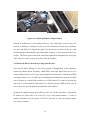
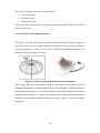
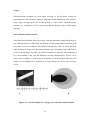
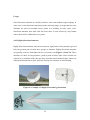
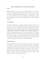
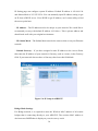
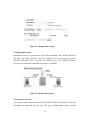
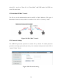
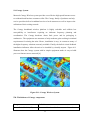
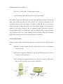
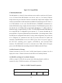
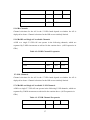
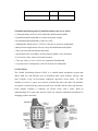
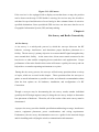
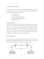
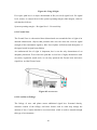
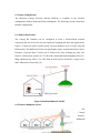
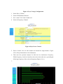
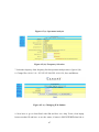
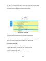
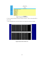
Internet and Data Connectivity Using
Optical Fiber and RF Signal
An Internship report presented in partial fulfillment of the requirements for the
degree of Bachelor of Science in Electronics and Telecommunication Engineering
SUBMITTED BY
Nurul Amin
ID: 071-19-609
SUPERVISED BY
A.K.M Fazlul Haque
Assistant Professor
Department of Electronics and Telecommunication Engineering
Daffodil International University
DAFFODIL INTERNATIONAL UNIVERSITY
DHAKA, BANGLADESH
©Daffodil International University
i
APPROVAL
This Internship titled “Internet and Data Connectivity using Optical fiber and RF Signal”
submitted by Nurul Amin to the Department of Electronics and Telecommunication
Engineering, Daffodil International University, has been accepted as satisfactory for the
partial fulfillment of the requirements for the degree of Bachelor of Science in
Electronics and Telecommunication Engineering and approved as to its style and
contents. The presentation was held on 27 February, 2011.
Board of Examiners
Dr. Md. Golam Mowla Chowdhury
Professor and Head
Department of Electronics and Telecommunication Engineering
Daffodil International University
--------------------(Chairman)
Dr. Subrata Kumar Aditya
Professor and Chairman
Department of Applied Physics
Dhaka University
------------------(External Member)
A.K.M Fazlul Haque
Assistant Professor
Department of Electronics and Telecommunication Engineering
Daffodil International University
--------------------(Internal Member)
Md. Mirza Golam Rashed
Assistant Professor
Department of Electronics and Telecommunication Engineering
Daffodil International University
-------------------(Internal Member)
©Daffodil International University
ii
DECLARATION
I hereby declare that the work presented in this Internship report titled “Internet and Data
Connectivity using Optical fiber and RF Signal” is done by us under the supervision of
Mr. A.K.M Fazlul Haque, Assistant Professor, Department of Electronics and
Telecommunication Engineering Daffodil International University, partial fulfillment of
the requirements for the degree of Bachelor of Science in Electronics and
Telecommunication Engineering. We also declare that this project is our original work.
As far as our knowledge goes, neither this report nor any part there has been submitted
elsewhere the award of any degree or diploma.
Supervised by:
A.K.M Fazlul Haque
Assistant Professor
Department of Electronics and Telecommunication Engineering
Daffodil International University
---------------(Signature)
Submitted by:
Nurul Amin
ID: 071-19-609
Department of Electronics and Telecommunication Engineering
Daffodil International University
---------------(Signature)
©Daffodil International University
iii
ACKNOWLEDGEMENT
First I express my heartiest thanks and gratefulness to almighty Allah for His divine
blessing makes us possible to complete this internship successfully.
I feel grateful to and wish my profound my indebtedness to Asst. Professor A.K.M Fazlul
Haque Department of ETE, Department of ETE Daffodil International University, Dhaka.
Deep Knowledge & keen interest of my supervisor in the field of wireless network
influenced us to carry out this project .His endless patience ,scholarly guidance ,continual
encouragement , constant and energetic supervision, constructive criticism , valuable
advice ,reading many inferior draft and correcting them at all stage have made it possible
to complete this project.
I would like to express my heartiest gratitude to Dr. Lutfur Rahman, Professor and Dean,
Faculty of science and information technology, Dr. Md. Golam Mowla Chowdhury
Professor and Head, Department of ETE, for his kind help to finish our internship report
and also to other faculty member and the staff of ETE department of Daffodil
International University.
I would like to thank my entire course mate in Daffodil International University, who
took part in this discuss while completing the course work.
Finally, I must acknowledge with due respect the constant support and patients of our
parents.
©Daffodil International University
iv
TABLE OF CONTENTS
CONTENTS
PAGES
Board of Examiners
ii
Declaration
iii
Acknowledgements
iv
Abstract
xi
CHAPTER
Chapter-1: Introduction
1.1 General Introduction
1
1.2 Objective of the present work
2
1.3 Organization of the project
2
Chapter-2: Optical Fiber Communication
2.1 Optical Fiber
3
2.2 History
3
2.2.1 First Generation
3
2.2.2 Second Generation
4
2.2.3 Third Generation
4
2.2.4 Forth Generation
4
2.3 Application
4
2.4 Technology
5
2.5 Material & Structure of Optical Fiber
5-6
2.6 Types of Optical Fiber
6
2.6.1 Multimode Optical Fiber
6-7
2.6.2 Single Mode Optical Fiber
8
2.6.3 Special-purpose Optical Fiber
8
Chapter-3: Optical Fiber Equipment & WAN Connectivity
3.1 Optical Time Domain Reflect Meter
9
3.1.1 Use of OTDR
9
3.1.2 Operation of OTDR
9-11
©Daffodil International University
v
3.2 Media Converter
11-12
3.3 Splicing Machine
12-13
3.4 Splicing Method
13
3.4.1 Stripping
13
3.4.2 Cleaving
14
3.4.3 Fusion
14-15
3.5 Internet & Data connectivity using Optical Fiber
15-16
Chapter-4: Radio Frequency
4.1 Radio Frequency
17
4.2 Radio Frequency Identification
17
4.2.1 Modulation
18
4.2.2 Demodulation
18
4.2.3 Radio Communication
18-19
4.3 Properties of RF signal
19
4.4 RF Antenna
19-20
4.4.1 Omni Directional Antenna
20-21
4.4.2 Semi Directional Antenna
21-22
4.4.3 High Directional Antenna
22-23
4.5 Antenna Gain
23
4.6 Antenna Spectrum
23-24
4.6. ITU Band
24-25
Chapter 5 RF Equipment
5.1 RF Equipment
26
5.2 AIRLIVE
26
5.2.1 AIRLIVE Features
26-27
5.2.2 Access Point Mode
27
5.2.3 Client Mode
27-28
5.3.4 Bridge Mode
28
5.4 Configuring of AIRLIVE
29-31
5.5 Bandwidth Control
31
5.5.1 Interface Control
©Daffodil International University
31-32
vi
5.5.2 Individual IP/MAC Control
32
5.5.3 Password Settings
32
5.6 Canopy System
33
5.6.1 Definitions of Canopy components
33-34
5.6.2 Types of BH Application
34
5.6.3 Security Feature
35
5.7 Backhaul (BH) Module
35-37
5.8 Bandwidth Management (Uplink/Downlink with Access Point)
37-38
5.9 GPS Meter
38
Chapter 6 Site Survey and Radio Connectivity
6.1 Site Survey
39
6.1.1 Preparing for a Site Survey
39-40
6.1.2 Outdoor Surveys
40
6.2 Line of Sight (LOS)
40
6.2.1 Fresnel Loss
41
6.2.2 Loss Due to Foliage
41
6.3 Canopy Configurations
41
6.3.1 Point-to-Point System
42
6.3.2 Point-to-Multipoint System
42-43
6.3.1 Channel Plans
43
6.3.2 RSSI
43
6.3.3 Custom RF Frequency Scan Selection List
43-44
6.3.4 Color Code
44
6.3.5 Downlink Data
44
6.3.6 High Priority Uplink Percentage
44
6.4 Radio link Point to Point AP/SM Configures
44-48
6.5 Configure Master End
48-49
Chapter-7: Conclusion
50
Reference
51
©Daffodil International University
vii
LIST OF FIGURES
FIGURES
PAGES
Chapter 2
Figure 2.1: Structure of Optical Fiber
6
Figure 2.2: Multimode Optical Fiber
7
Figure2.3: Graded-index fiber
7
Figure2.4: Single mode Fiber
8
Chapter 3
Figure 3.1: Block Diagram of OTDR
10
Figure 3.2: Fiber Media Converter
11
Figure 3.3: Splicing Machine
12
Figure 3.4: Splicing Method of Optical Fiber
13
Figure 3.5: Splicing Method of Optical Fiber
14
Figure 3.6: Splicing Method of Optical Fiber
15
Figure 3.7: Data Connectivity using optical Fiber
16
Chapter 4
Figure 4.1: Dipole doughnut & Omni Directional Antenna
20
Figure 4.2 :(A& B) Sample & Coverage area semi-directional antennas
21
Figure 4.3: Sample of a highly directional grid antenna
22
Figure 4.4: Radiation pattern of a highly directional antenna
22
Chapter 5
Figure 5.1: Air live setup
27
Figure 5.2: Access Point Mode
27
Figure 5.3: Clients mode
28
Figure 5.4: Bridge Mode Of AIRLIVE
28
Figure 5.5: IP Setup
29
Figure 5.6: IP Setup in AIRLIVE
30
Figure 5.7: Bridge Mode setting
31
Figure 5.8: Bandwidth Control
31
Figure 5.9: IP & MAC Control
32
Figure 5.10: Password setting
32
©Daffodil International University
viii
Figure 5.11: Canopy Wireless System
33
Figure 5.12: Canopy BH Base
35
Figure 5.13: GPS meter
39
Chapter 6
Figure 6.1: Ling of Sight
40
Figure 6.2: Fresnel zone
41
Figure 6.3: Point to Point system CANOPY
42
Figure 6.4: Point-to-Multipoint system of CANOPY
42
Figure 6.5: Block Diagram of RF connectivity
45
Figure 6.5 (a): Canopy Configuration
45
Figure 6.5(b): Power Control
46
Figure 6.5 (c): Spectrum Analysis
46
Figure 6.5 (d): Frequency Selection
47
Figure 6.5 (e): Changing IP & Subnet
47
Figure 6.5 (f): Link Status
48
Figure 6.5 (g): Link Efficiency
48
Figure 6.5(h): Point to Point test
49
©Daffodil International University
ix
LIST OF TABLES
TABLES
PAGES
Table 3.1: The theoretical interaction of pulse width
10
Table 4.1: ITU Radio Frequency
24-25
Table 4.2: IEEE Frequency Band
25
Table 4.1:2.4 BH Channel Frequencies
36
Table 4.2:5.2 BH Channel Frequencies
37
Table 4.3: 5.7 BH Channel Frequencies
37
©Daffodil International University
x
Abstract
This report presents the Internet and Data Connectivity using Optical Fiber and RF
Signal, especially for RANKS ITT LTD. This kind of connectivity helps the whole nation
or multi-company to provide best quality of service to the consumer. Using optical fiber,
it is possible to connect the clients’ device by means of media converter. To perform this
conversion, some essential devices such as optical fiber, media converter, OTDR and
splicing machine have been used. Point to point connection by means of Canopy, Airlive
has been used for client satisfaction. In this report, the requirements of installation &
configuration are also described. Bandwidth controlling system has also been considered
to optimize the performance of the system.
©Daffodil International University
xi
Chapter 1
Introduction
1.1 GENERAL INTRODUCTION
I have completed my internship successfully in Ranks ITT. Ranks ITT is the largest
data network in terms of geographic coverage in Bangladesh, spanning 6 Divisions
and 64 Districts with 30 PoPs nationwide. Operating on a single platform using RAD
and Cisco technology, the Network offers a broad range of voice and data solutions to
nationals and multinationals in a variety of industries. Ranks - ITT is the market
leader of nation wide data communication network service with over USD 4 million
investments. Under a strategic infrastructure sharing agreement with Grameenphone
(GP), Ranks - ITT retails excess capacity of 1,945 km of GP Fiber Optics Network in
62 districts and operates over 30 Point-of-Presence (PoP) through out Bangladesh.
As a single integrated national network, services are fully managed from end-to-end.
Offered on an unrivaled national scale, these include business intranet and Internet
solutions, high performance remote access services over local fixed or dial-up lines,
and many other Wide Area Network services. As the technology leader Ranks - ITT
combines its carrier class technology deployment and national coverage with superior
A world-wide research network sharing a common addressing scheme and using the
TCP/IP software protocol for data transfer between hosts. It is composed of many
individual campuses, state, national, and regional networks. In computer science, data
is information in a form suitable for use with a computer. Data is often distinguished
from programs. A program is a set of instructions that detail a task for the computer to
perform. First, I understood the background of the core network of the company then
applied to perform the problem statement and finally checked the status of network
whether it was operative. In this report, the overall all theoretical and technical details
of the given company have been introduced and finally the problem solution of the
project has been tested and verified using simulation tool.
1
1.2 Objective of the work
To provide internet and data service using optical fiber we use various devices such as
media converter, OTDR, Splicing Machine.
For Clients requirement we provide wireless connectivity. In wireless system, we use
various devices such as Canopy, AIRLIVE, and GPS. The require installation &
configuration are describe in this report.
1.4 Organization of the Report
This internship report has seven chapters in total
Chapter 1 reviews on the Introduction of this internship report, definition of the internet and
data, how to provide internet and data service.
Chapter 2 reviews of optical fiber communication, history, Application of the optical fiber,
Material of optical fiber, types of optical fiber
Chapter 3 reviews Optical fiber equipment, Describer and configuration of optical fiber
device, also show the process of data service
Chapter 4 reviews of RF signal, Modulation & Demodulation, types of antenna
Chapter 5 review of RF equipment, Describe about RF devices
Chapter 6 reviews of Site survey RF connectivity. In this chapter also describe how
configure the radio device
Chapter 7 brings out the conclusion of the entire work
2
Chapter 2
Optical Fiber Communication
2.1 Optical Fiber
An optical fiber or optical fibre is a thin, flexible, transparent fiber that acts as a
waveguide, or "light pipe", to transmit light between the two ends of the fiber. The
field of applied science and engineering concerned with the design and application of
optical fibers is known as fiber optics. Optical fibers are widely used in fiber-optic
communications, which permits transmission over longer distances and at higher
bandwidths (data rates) than other forms of communication. Fibers are used instead of
metal wires because signals travel along them with less loss and are also immune to
electromagnetic interference. Fibers are also used for illumination, and are wrapped in
bundles so they can be used to carry images, thus allowing viewing in tight spaces.
Specially designed fibers are used for a variety of other applications, including
sensors and fiber lasers.
2.2 History
In 1966 Charles K. Kao and George Hockham proposed optical fibers at STC
Laboratories (STL) at Harlow, England, when they showed that the losses of 1000
dB/km in existing glass (compared to 5-10 db/km in coaxial cable) was due to
contaminants, which could potentially be removed.
Optical fiber was successfully developed in 1970 by Corning Glass Works, with
attenuation low enough for communication purposes (about 20dB/km). After a period
of research starting from 1975, the first commercial fiber-optic communications
system was developed.[1]
2.2.1 First-generation
This first-generation system operated at a bit rate of 45 Mbps with repeater spacing of
up to 10 km. Soon on 22 April, 1977, General Telephone and Electronics sent the first
live telephone traffic through fiber optics at a 6 Mbit/s throughput in Long Beach,
California
3
2.2.2 Second generation
The second generation of fiber-optic communication was developed for commercial
use in the early 1980s, operated at 1.3 µm, and used In GaAsP semiconductor .The bit
rates of up to 1.7 Gb/s with repeater spacing up to 50 km.
2.2.3 Third-generation
Third-generation fiber-optic systems operated at 1.55 µm and had losses of about
0.2 dB/km. They achieved this despite earlier difficulties with pulse-spreading at that
wavelength using conventional In GaAsP semiconductor lasers. These developments
eventually allowed third-generation systems to operate commercially at 2.5 Gbit/s
with repeater spacing in excess of 100 km.
2.2.4 Fourth generation
The fourth generation of fiber-optic communication systems used optical
amplification to reduce the need for repeaters and wavelength division multiplexing to
increase data capacity.. Recently, bit-rates of up to 14 Tbit/s have been reached over a
single 160 km line using optical amplifiers.
2.3 Applications
Optical fiber is used by many telecommunications companies to transmit telephone
signals, Internet communication, data transmission, and cable television signals. Due
to much lower attenuation and interference, optical fiber has large advantages over
existing copper wire in long-distance and high-demand applications.
Since 1990, when optical-amplification systems became commercially available, the
telecommunications industry has laid a vast network of intercity and transoceanic
fiber communication lines. By 2002, an intercontinental network of 250,000 km of
submarine communications cable with a capacity of 2.56 Tb/s was completed, and
although specific network capacities are privileged information, telecommunications
investment reports indicate that network capacity has increased dramatically since
2004.
4
2.4 Technology
Modern fiber-optic communication systems generally include an optical transmitter to
convert an electrical signal into an optical signal to send into the optical fiber, a cable
containing bundles of multiple optical fibers that is routed through underground
conduits and buildings, multiple kinds of amplifiers, and an optical receiver to recover
the signal as an electrical signal..
2.5 Material & Structure of Optical Fiber
An optical fiber consists of a core, cladding, and a buffer (a protective outer coating),
in which the cladding guides the light along the core by using the method of total
internal reflection. The core and the cladding (which has a lower-refractive-index) are
usually made of high-quality silica glass, although they can both be made of plastic as
well.
The core of a conventional optical fiber is a cylinder of glass or plastic that runs along
the fiber's length. The core is surrounded by a medium with a lower index of
refraction, typically a cladding of a different glass, or plastic. Light traveling in the
core reflects from the core-cladding boundary due to total internal reflection, as long
as the angle between the light and the boundary is less than the critical angle. As a
result, the fiber transmits all rays that enter the fiber with a sufficiently small angle to
the fiber's axis. The limiting angle is called the acceptance angle, and the rays that are
confined by the core/cladding boundary are called guided rays.
The core is characterized by its diameter or cross-sectional area. In most cases the
core's cross-section should be circular, but the diameter is more rigorously defined as
the average of the diameters of the smallest circle that can be circumscribed about the
core-cladding boundary, and the largest circle that can be inscribed within the corecladding boundary. This allows for deviations from circularity due to manufacturing
variation. [1]
Another commonly-quoted statistic for core size is the mode field diameter. This is
the diameter at which the intensity of light in the fiber falls to some specified fraction
of maximum (usually 1/e2≈13.5%). For single-mode fiber, the mode field diameter is
5
larger than the physical diameter of the core, because the light penetrates slightly into
the cladding as an evanescent wave.
The structure of a typical single-mode
fiber
1.Core 8 µm diameter
2.Cladding 125 µm dia
3.Buffer 250 µm dia
4.Jacket 400 µm dia
Figure 2.1: Structure of Optical Fiber
2.6 Types of Optical Fiber
Two main types of optical fiber used in optic communications include multi-mode
optical fibers and single-mode optical fibers. A multi-mode optical fiber has a larger
core (≥ 50 micrometers), allowing less precise, cheaper transmitters and receivers to
connect to it as well as cheaper connectors. The core of a single-mode fiber is smaller
(<10 micrometers) and requires more expensive components and interconnection
methods, but allows much longer, higher-performance links.
2.6.1 Multi-mode Optical Fiber
The propagation of light through a multi-mode optical fiber a laser bouncing down an
acrylic rod, illustrating the total internal reflection of light in a multi-mode optical
fiber. Fiber with large core diameter may be analyzed by geometrical optics. Such
fiber is called multi-mode fiber, from the electromagnetic analysis. In a step-index
multi-mode fiber, rays of light are guided along the fiber core by total internal
reflection [1]
Rays that meet the core-cladding boundary at a high angle, greater than the critical
angle for this boundary, are completely reflected. The critical angle (minimum angle
for total internal reflection) is determined by the difference in index of refraction
between the core and cladding materials
6
Figure 2.2: Multimode Optical Fiber
Rays that meet the boundary at a low angle are refracted from the core into the
cladding, and do not convey light and hence information along the fiber. The critical
angle determines the acceptance angle of the fiber, often reported as a numerical
aperture. A high numerical aperture allows light to propagate down the fiber in rays
both close to the axis and at various angles, allowing efficient coupling of light into
the fiber.
Figure2.3: Graded-index fiber
In graded-index fiber, the index of refraction in the core decreases continuously
between the axis and the cladding. This causes light rays to bend smoothly as they
approach the cladding, rather than reflecting abruptly from the core-cladding
boundary. The resulting curved paths reduce multi-path dispersion because high angle
rays pass more through the lower-index periphery of the core, rather than the highindex center. This ideal index profile is very close to a parabolic relationship between
the index and the distance from the axis.
7
2.6.2 Single-Mode Optical Fiber
Fiber with a core diameter less than about ten times the wavelength of the propagating
light cannot be modeled using geometric optics. The electromagnetic analysis may
also be required to understand behaviors such as speckle that occur when coherent
light propagates in multi-mode fiber. As an optical waveguide, the fiber supports one
or more confined transverse modes by which light can propagate along the fiber. Fiber
supporting only one mode is called single-mode or mono-mode fiber.[2]
Figure2.4: Single mode Fiber
The waveguide analysis shows that the light energy in the fiber is not completely
confined in the core. Instead, especially in single-mode fibers, a significant fraction of
the energy in the bound mode travels in the cladding as an evanescent wave. he most
common type of single-mode fiber has a core diameter of 8–10 micrometers and is
designed for use in the near infrared. The mode structure depends on the wavelength
of the light used, so that this fiber actually supports a small number of additional
modes at visible wavelengths. Multi-mode fiber, by comparison, is manufactured with
core diameters as small as 50 micrometers and as large as hundreds of micrometers.
2.6.3 Special-purpose Optical Fiber
Some special-purpose optical fiber is constructed with a non-cylindrical core and/or
cladding layer, usually with an elliptical or rectangular cross-section. These include
polarization-maintaining fiber
8
Chapter 3
Optical Fiber Equipment & WAN Connection
3.1 Optical Time-Domain Reflect Meter
Optical Time-Domain Reflect Meter (OTDR) is an optoelectronic instrument used to
characterize an optical fiber. An OTDR injects a series of optical pulses into the fiber
under test. It also extracts, from the same end of the fiber, light that is scattered
(Rayleigh Backscatter) or reflected back from points along the fiber. The strength of
the return pulses is measured and integrated as a function of time, and is plotted as a
function of fiber length. [2]
3.1.1 Uses of OTDR
OTDR are commonly used to characterize the loss and length of fibers as they go
from initial manufacture, through to cabling, warehousing while wound on a drum,
installation and then splicing. The last application of installation testing is more
challenging, since this can be over extremely long distances, or multiple splices
spaced at short distances, or fibers with different optical characteristics joined
together. OTDR are also commonly used for fault finding on installed systems. In
this case, reference to the installation OTDR trace is very useful, to determine where
changes have occurred. .
3.1.2 Operation of OTDR
OTDR are available with a variety of fiber types and wavelengths, to match common
applications. In general, OTDR testing at longer wavelengths such as 1550 nm or
1625 nm, can be used to identify fiber attenuation caused by fiber problems, as
opposed to the more common splice or connector losses. The optical dynamic range
of an OTDR is limited by a combination of optical pulse output power, optical pulse
width, input sensitivity, and signal integration time.
A longer laser pulse improves dynamic range and attenuation measurement resolution
at the expense of distance resolution. For example, using a long pulse length, it may
possible to measure attenuation over a distance of more than 100 km, however in this
9
case an optical event may appear to be over 1 km long. A short pulse length will
improve distance resolution of optical events, but will also reduce measuring range
and attenuation measurement resolution. The "apparent measurement length" of an
optical event is referred to as the "dead zone". The theoretical interaction of pulse
width and dead zone can be summarized as follows
Table 3.1: The theoretical interaction of pulse width
Pulse length
Event Dead zone
1 nsec
0.15 m ( theoretically)
10 nsec
1.5 m ( theoretically )
100 nsec
15 m
1 µsec
150 m
10 µsec
1.5 km
100 µsec
15 km
Dead Zone
Dead zone is classified in two ways. Firstly, an "Event Dead Zone" is related to a
reflective discrete optical event
Figure 3.1: Block Diagram of OTDR
In this situation, the measured dead zone will depend on a combination of the pulse
length and the size of the reflection. Secondly, an "Attenuation Dead Zone" is related
to a non-reflective event.
10
The theoretical distance measuring accuracy of an OTDR is extremely good, since it
is based on software and a crystal clock with an inherent accuracy of better than
0.01%. OTDR excels at identifying the existence of unacceptable point loss or return
loss in cables. Its ability to accurately measure absolute end-to-end cable loss or
return loss can be quite poor, so cable acceptance usually includes an end to end test
with a light source and power meter, and optical return loss meter.
3.2 Fiber Media Converter
Fiber media converters are simple networking devices that make it possible to connect
two dissimilar media types such as twisted pair with fiber optic cabling. They were
introduced to the industry nearly two decades ago, and are important in
interconnecting fiber optic cabling-based systems with existing copper-based,
structured cabling systems.
Media conversion types
Fiber media converters support many different data communication protocols
including Ethernet, Fast Ethernet, Gigabit Ethernet, T1/E1/J1, DS3/E3, as well as
multiple cabling types such as coax, twisted pair, multi-mode and single-mode fiber
optics.
Simple Network Management Protocol (SNMP) enables proactive management of
link status, monitoring chassis environmental statistics and sending traps to network
managers in the event of a fiber break or even link loss on the copper port. Fiber
media converters can connect different Local area network (LAN) media, modifying
duplex and speed settings. Switching media converters can connect legacy 10BASE-T
network segments to more recent 100BASE-TX or 100BASE-FX Fast Ethernet
Infrastructure.
Figure 3.2: Fiber Media Converter
11
For example, existing Half-Duplex hubs can be connected to 100BASE-TX Fast
Ethernet network segments over 100BASE-FX fiber
Media converters can extend the reach of the LAN over single-mode fiber up to 130
kilometers with 1550 nm optics. As well as conventional dual strand fiber converters,
with separate receive and transmit ports, there are also single strand fiber converters,
which can extend full-duplex data transmission up to 70 kilometers over one optical
fiber.
3.3 Splicing Machine
If you want to join two lengths of optical fiber together with the least possible loss of
optical power, the method to choose is fusion splicing. In fusion splicing, the cores
and claddings of the two fibers are actually melted together. Because the core has a
very small diameter, it requires a very precise instrument to join the cores in a way
that lets the most light pass through the point of joining. (For single mode fiber, the
diameter is about 1/100 of a millimeter. For multimode fiber, the diameter is 1/16 of a
millimeter.)
Figure 3.3: Splicing Machine
The new rugged construction adds improved reliability by resisting shock, dust, and
rain, and can withstand a 30” drop test. The splices a fiber in 8-10 seconds and heats a
60mm splice sleeve in 30-40 seconds, for a total cycle time of only 39-45 seconds.
New features, such as automatic tube heater operation, user-selectable clamping
method, automated monitor image orientation, and battery charge capability during
splice operation provide the end user a productivity tool they can count on. New
12
software included provides the ability to download splice data to a PC for splice data
reporting, download splice operating software via the internet to maintain peak
performance, and download video images from the splice to enhance technical
support.
3.4 Splicing Method
A fusion splice is a way of joining two fiber cores by melting the ends together using
an electric arc. A splicing machine is used because an extremely high degree of
accuracy is needed; the machine first has to align the cores and then apply the exact
amount of heat to melt the ends before pressing them together. Splicing can be carried
out using a mechanical splice but these only hold the fiber ends together, precisely
aligned but not permanently joined. [3]
There are four basic steps to
fusion splicing
1 - Strip backs all coatings
down to the bare fibers and
cleans using isopropyl
alcohol.
2 - Cleave the fibers using a
precision cleaving tool and
put the heat shrink tube on
to one of the ends.
3 - Fuse the fibers
together in the fusion
splice.
Figure 3.4: Splicing Method of Optical Fiber
4 - Put the heat shrink
protector on the fiber joint.
3.4.1 Stripping
Strip back the external sheathing of the cable using a rotary stripping tool. Cut back
the agamid strength member using ceramic or Kevlar scissors. Strip the primary
13
buffer from the fiber using fiber strippers not ordinary wire strippers. Do this a small
section at a time to prevent the fiber breaking, about 10mm (3/8 in) on each cut is fine
until you get used to it. Strip back about 35mm (1.5 in).
3.4.2 Cleaving
The cleaver first scores the fiber and then pulls the fiber apart to make a clean break.
It is important that the ends are smooth and perpendicular to get a good joint, this is
why a hand held cleaver will not do. Basically the operation consists of putting the
fiber into the groove and clamping, then close the lid and press the lever
Figure 3.5: Splicing Method of Optical Fiber
3.4.3 The Fusion Process
Once the fiber ends are prepared they are placed in the fusion splicer. Press the button
and the machine takes care of the rest of the fusion process automatically. Figure 2.7
this on the photo where a much magnified image shows the two fiber ends. The
display also shows how well the cleaver does its job of producing a perfect 90 degree
cut. If you watch very carefully in the video you can see the X and Y alignment that
takes place. The splice aligns the fibers on one axis and then from another camera
angle set at 90 degrees, it aligns the other axis.
14
Figure 3.6: Splicing Method of Optical Fiber
Bearing in mind that we are dealing with two very small glass rods of only 125
microns in diameter, it brings it home as to how extremely accurate these machines
are. Once the fibers are aligned the splice fires an electric arc between the two ends
which melts them immediately and pushes them together, or fuses them into one piece
of fiber. The fusion splices then tests for dB loss and tensile strength before giving the
"OK" beeps for you to remove the splice from the machine
3.5 Internet & Data Connectivity Using Optical Fiber
Now Present Share Business is the most popular in Bangladesh. In this Business
control By Dhaka Stock Exchange (DSE).DSE need high Speed data service for
online trading. Because sell or buy signal updated in nanosecond .In this System DSE
uses Main Frame Server. In DSE up to 3000 Branch & Sub Branch connected to DSE
server directly or via head office main server. DSE selected 5 Vendor for provide the
data service in the branch & sub branch. For Security propose DSE provide own IP
series. They also provide branch & sub branch in IP Address.
Example Greenland Security head office by runs 3 pc. He has also other 3 sub branch.
IP address for head office 150.1.236.3/28 (236 is the branch number 3 is the pc
number).IP address for sub branch 155.236.2.1/24 (here 2 is the sub branch number
&1 is the pc number)
15
Figure 3.7: Data Connectivity using optical Fiber
1. Sub Branch to Dhanmondi Pop connected by Optical Fiber.
2. Dhanmoni to Motijheel Pop is the backbone
3. Motijheel to Clients MSA Connected By Optical fiber
4. Cliens MSA to DSE NOC Connected by UTP Cable
5. DSE NOC to DSE MFS connected by UTP Cable
6. For online trading need minimum 256 kbps speed
For path test first need check pop gateway than need to check head office MSA
Gateway. If every thing then we need to test DSE MFS Server
16
Chapter 4
Radio Frequency
4.1 Radio Frequency
Radio frequency (abbreviated RF, rf, orr.f.) is a term that refers to alternating current
(AC) having characteristics such that, if the current is input to an antenna, an
electromagnetic (EM) field is generated suitable for wireless broadcasting and/or
communications. These frequencies cover a significant portion of the electromagnetic
radiation spectrum, extending from nine kilohertz (9 kHz),the lowest allocated
wireless communications frequency (it's within the range of human hearing), to
thousands of gigahertz(GHz).
Radio frequency (RF) is a rate of oscillation in the range of about 30 kHz to 300 GHz,
which corresponds to the frequency of electrical signals normally used to produce and
detect radio waves. RF usually refers to electrical rather than mechanical oscillations,
although mechanical RF systems do exist
4.2 Radio-frequency identification
Radio-frequency identification (RFID) is a technology that uses communication via
radio waves to exchange data between a reader and an electronic tag attached to an
object, for the purpose of identification and tracking. Some tags can be read from
several meters away and beyond the line of sight of the reader. The application of
bulk reading enables an almost parallel reading of tags. Radio-frequency
identification involves interrogators (also known as readers), and tags (also known as
labels).
Most RFID tags contain at least two parts. One is an integrated circuit for storing and
processing information, modulating and demodulating a radio-frequency (RF) signal,
and other specialized functions. The other is an antenna for receiving and transmitting
the signal. The first patent to be associated with the abbreviation RFID was granted to
Charles Walton in 1983
17
4.2.1 Modulation
In telecommunications, modulation is the process of conveying a message signal, for
example a digital bit stream or an analog audio signal, inside another signal that can
be physically transmitted. Modulation of a sine waveform is used to transform a base
band message signal to a pass band signal, for example a radio-frequency signal (RF
signal). In radio communications, cable TV systems or the public switched telephone
network for instance, electrical signals can only be transferred over a limited pass
band frequency spectrum, with specific (non-zero) lower and upper cutoff
frequencies. Modulating a sine wave carrier makes it possible to keep the frequency
content of the transferred signal as close as possible to the centre frequency (typically
the carrier frequency) of the pass band. When coupled with demodulation, this
technique can be used to, among other things, transmit a signal through a channel
which may be opaque to the base band frequency range (for instance, when sending a
telephone signal through a fiber-optic strand)
4.2.2 Demodulation
Demodulation is the act of extracting the original information-bearing signal from a
modulated carrier wave. A demodulator is an electronic circuit (or computer program
in a software defined radio) that is used to recover the information content from the
modulated carrier wave. These terms are traditionally used in connection with radio
receivers, but many other systems use many kinds of demodulators. Another common
one is in a modem, which is a contraction of the terms modulator/demodulator.
4.2.3 Radio communication
In order to receive radio signals an antenna must be used. However, since the antenna
will pick up thousands of radio signals at a time, a radio tuner is necessary to tune in
to a particular frequency (or frequency range). This is typically done via a resonator –
in its simplest form, a circuit with a capacitor and an inductor forming a tuned circuit.
Often the inductor or the capacitor of the tuned circuit is adjustable allowing the user
to change the frequencies at which it resonates. The resonant frequency of a tuned
circuit is given by the formula
18
Where f 0 is the frequency in hertz, L is inductance in henries, and C is capacitance in
farads
4.3 Special properties of RF electrical signals
Electrical currents that oscillate at RF have special properties not shared by direct
current signals. One such property is the ease with which they can ionize air, creating
a conductive path through it. This property is exploited by 'high frequency' units used
in electric arc welding, although strictly speaking these machines do not typically
employ frequencies within the HF band.
Another special property is that RF current cannot penetrate deeply into electrical
conductors but flows along the surface of conductors; this is known as the skin effect.
Another property is the ability to appear to flow through paths that contain insulating
material, like the dielectric insulator of a capacitor. The degree of effect of these
properties depends on the frequency of the signals
4.4 RF Antennas
An RF antenna is a device used to convert high frequency (RF) signals on a
transmission line (a cable or waveguide) into propagated waves in the air. The
electrical fields emitted from antennas are called beams or lobes. Antennas generally
deal in the transmission and reception of radio waves, and are a necessary part of all
radio equipment. Antennas are used in systems such as radio and television
broadcasting, point-to-point radio communication, wireless LAN, cell phones, radar,
and spacecraft communication. Antennas are most commonly employed in air or outer
space, but can also be operated under water or even through soil and rock at certain
frequencies for short distances. The physical dimensions of an antenna, such as its
length, are directly related to the frequency at which the antenna can propagate waves
or receive propagated waves. The physical structure of an antenna is directly related
to the Shape of the area in which it concentrates most of its related RF energy.
19
There are three generic categories of RF antennas:
1. Omni-directional
2. Semi-directional
3. Highly-directional
Each category has multiple types of antennas, each having different RF characteristics
and appropriate uses.
4.4.1 Omni-directional (Dipole) Antenna
The dipole is an omni- directional antenna, because it radiates its energy equally in all
directions around its axis. Dipole antenna is Simple to design; dipole antenna is
standard equipment on most access points. Directional antennas concentrate their
energy into a cone, known as a "beam."
Figure 4.1: Dipole doughnut & Omni Directional Antenna
Figure shows that the dipole's radiant energy is concentrated into a region that like a
doughnut, with the dipole vertically through the "hole" of the "doughnut." signal from an omnidirectional antenna radiates in a 360-degree horizontal. If an antenna radiates in all directions
equally (forming a sphere), it is called an 3pic radiator, which is the theoretical reference for
antennas, but rather, practical antennas all have some type of gain over that of an isotropic
radiator.[4]
20
Usages
Omni-directional antennas are used when coverage in all directions around the
horizontal axis of the antenna is required. Omni-directional antennas are most effective
where large coverage areas are needed around a central point. Omni-directional
antennas are commonly used for point-to-multipoint designs with a hub-n-spoke
topology.
4.4.2 Semi directional Antenna
Semi directional antennas direct the energy from the transmitter significantly more in
one particular direction rather than the uniform circular pattern that is common with
the Omni- directional antenna; Semi-directional antennas come in many different
styles and shapes. Some semi- directional antennas types frequently used with wireless
LANs are Patch, Panel, antennas. All of these antennas are generally flat and designed
for wall mounting. Each type has different coverage characteristics. Figure 3.6(A)
shows some examples of semi-directional antennas. Semi-directional antennas often
radiate in a hemispherical or cylindrical coverage pattern as can be seen in Figure
3.6(B)
A
B
Figure 4.2 :( A& B) Sample & Coverage area semi-directional antennas
21
Usages
Semi-directional antennas are ideally suited for short and medium range bridging. In
some cases, semi-directional antennas provide such long-range coverage that they may
eliminate the need for multiple access points in a building. In some cases, semidirectional antennas have back and side lobes that, if used effectively, may further
reduce the need for additional access points.
4.4.3 Highly directional antenna
Highly-directional antennas emit the most narrow signal beam of any antenna type and
have the greatest gain of these three groups of antennas. Highly-directional antennas
are typically concave, dish-shaped devices, as can be seen Figures 3.3 and 3.4. These
antennas are ideal for long distance, point-to-point wireless links. Some models are
referred to as parabolic dishes because they resemble small satellite dishes. Others are
called grid antennas due to their perforated design for resistance to wind loading.
Figure 4.3: Sample of a highly directional grid antenna
22
Figure 4.4: Radiation pattern of a highly directional antenna
Usages
High-gain antennas do not have a coverage area that client devices can use. These are
used for point-to-point communication links, and can transmit at up to 25 miles.
Potential uses of highly directional antennas might be to two buildings that are miles
away from each other but have no obstructions in path. Additionally, these antennas
can be aimed directly at each other within a building in order to "blast" through an
obstruction.
4.5 Antenna Gain
An antenna element without the amplifiers and filters typically associated with it is a
passive device. There is no conditioning, amplifying, or manipulating of the signal by
antenna element itself. The antenna can create the effect of amplification by virtue of
its physical shape. Antenna amplification is the result of focusing the RF radiation into
a tighter beam, just as the bulb of a flashlight can be focused into a tighter beam —
eating a seemingly brighter light source that sends the light further. The focusing of
radiation measured by way of beam widths, which are measured in degrees horizontal
and vertical. For example, an omni-directional antenna has a 360-degree horizontal
beam width. By limiting the 360-degree beam width into a more focused beam of, say,
30 degrees, at the same power, the RF waves will be radiated further.
4.6 Radio Spectrum
Radio spectrum refers to the part of the electromagnetic spectrum corresponding to
radio frequencies – that is, frequencies lower than around 300 GHz (or, equivalently,
wavelengths longer than about 1 mm). Different parts of the radio spectrum are used
for different radio transmission technologies and applications. Radio spectrum is
typically government regulated in developed countries, and in some cases is sold or
licensed to operators of private radio transmission systems (for example, cellular
telephone operators or broadcast television stations).
23
A band is a small section of the spectrum of radio communication frequencies, in
which channels are usually used or set aside for the same purpose.
4.6.1 ITU
The ITU radio bands are designations defined in the ITU Radio Regulations. Table
3.1 states that "the radio spectrum shall be subdivided into nine frequency bands,
which shall be designated by progressive whole numbers” in accordance with the
following table.
Table 4.1: ITU Radio Frequency
Band
Symbols
Number
1
2
Frequency
Wavelength Range
Typical sources
Range
Extremely
3 to 30 Hz
10,000 to 100,000 km deeply-submerged
Low
submarine
Frequency
communication
Super Low 30 to 300 Hz
1000 to 10,000 km
Frequency
submarine
communication, ac
power grids
3
Ultra Low 300 to 3 kHz
100 to 1000 km
Frequency
earth quakes, earth
mode
communication
4
Very Low 3 to 30 kHz
10 to 100 km
Frequency
near-surface
submarine
communication,
5
Low
30 to 300 kHz
1 to 10 km
Frequency
6
Medium
High
broadcasting,
aircraft beacons
300 to 3000 kHz
100 to 1000 m
Frequency
7
AM
AM
broadcasting,
aircraft beacons
3 to 30 MHz
10 to 100 m
Frequency
Skywave long
range radio
communication:
24
8
Very High 30 to 300 MHz
1 to 10 m
Frequency
FM radio broadcast,
television
broadcast,
9
Ultra High 300 to 3000 MHz 10 to 100 cm
PMR, television
Frequency
broadcast,GPS,
mobile phone
communication
10
Super High 3 to 30 GHz
1 to 10 cm
Frequency
DBS
WLAN
satellite
(Wi-Fi
802.11 a)
11
Extra High 30 to 300 GHz
1 to 10 mm
Frequency
WiMAX,
high
resolution radar,
Table 4.2: IEEE Frequency Band
Band
Frequency
Origin of name
range
HF
3 to 30 MHz
High Frequency
VHF
30 to 300 MHz
Very High Frequency
UHF
300 to 1000 MHz
Ultra High Frequency
L band
1 to 2 GHz
Long wave
S band
2 to 4 GHz
Short wave
C band
4 to 8 GHz
Compromise between S and X
X band
8 to 12 GHz
Used in WW II for fire control, X for cross (as in
crosshair)
K u band
12 to 18 GHz
Kurz-under
K band
18 to 27 GHz
German Kurz (short)
K a band
27 to 40 GHz
Kurz-above
V band
40 to 75 GHz
W band
75 to 110 GHz
W follows V in the alphabet
mm band 110 to 300 GHz
25
Chapter 5
RF Equipment
5.1 RF Equipment
1. Radio Device( AIRLIVE Canopy )
2. Reflector
3. GPS
5.2 AIRLIVE
The Airlive is a wireless outdoor multi-function device based on IEEE 802.11g/b
2.4GHz radio technologies. When installed in upright position, it is rain and splash
proof. It features an integrated 10dBi patch antenna and passive POE to simplify the
installation. The built-in antenna can provide up to 3km of distance depending on
conditions.[7]
5.2.1 AIRLIVE Features
󲐀 802.11g/b Hi Powered Chipset
󲐀 4MB Flash and 16MB SDRAM
󲐀 9 wireless multi-function modes: Access Point, Client Mode, WDS Repeater, WDS
Bridge, Universal Repeater, WISP Router, AP Router, WISP+ Universal Repeater,
WDS Station
󲐀 10Bi Integrated Patch Antenna: Vertical Polarization. 70 degree Horizontal and 38
Degree Vertical coverage in the forward direction
󲐀 Power by passive PoE: 12V Adapter and injector included
󲐀 Slide out housing design for easy maintenance
󲐀 Pole Mount strap included. Optional metal mount and wall mount available
󲐀 Interface and IP/MAC Bandwidth Control
󲐀 Site Survey, Signal Survey, and Signal Strength LED indicator
󲐀 Clear Signal Interference Resistant Technology
26
󲐀 Emergency firmware recovery mode
󲐀 Web, HTTPS, SSH, Telnet managements
Figure 5.1: Air live setup
5.2.2 Access Point Mode
When operating in the Access Point mode, the AIR live becomes the center hub of the
wireless network. All wireless cards and clients connect and communicate through
AIRLIVE. This type of network is known as “Infrastructure network”. Other
AIRLIVE or 802.11a CPE can connect to AP mode through “Client Mode”.
Figure 5.2: Access Point Mode
5.2.3 Client Mode
This mode is also known as “Client” mode. For AIRLIVE, there are 2 types of Client
modes: Infrastructure and Ad hoc mode. In Infrastructure mode, the AIRLIVE acts as
if it is a wireless adapter to connect with a remote Access Point. Users can attach a
27
computer or a router to the LAN port of AIRLIVE to get network access. This mode
is often used by WISP on the subscriber’s side.[7]
Figure 5.3: Clients mode
In Client Ad Hoc mode, AIRLIVE can connect to other wireless adapters without
access point. Users can attach a computer or a router to the LAN port of AIRLIVE to
get network access.
5.3.4 Bridge Mode
This mode is also known as “WDS Pure MAC Bridge mode”. When configured to
operate in the Wireless Distribution System (WDS) Mode, the AIRLIVE provides
bridging functions with remote LAN networks in the WDS system. The system will
support up to total of 8 bridges in a WDS network. However, each bridge can only
associate with maximum of 4 other bridges in the WDS configuration. This mode is
best used when you want to connect LAN networks together wirelessly. If you have
more than 2 AP in WDS Bridges mode, please remember to turn on the “802.1d
Spanning Tree” or “STP” option on to avoid network loop. This mode usually
delivers faster performance than infrastructure mode. Figure 4.4
28
Figure 5.4: Bridge Mode of AIRLIVE
5.4 Configuring of AIRLIVE
The AIRLIVE can be managed remotely by a PC through either the wired or wireless
network. The default IP address of the AIRLIVE is 192.168.1.1 with a subnet mask of
255.255.255.0. This means the IP address of the PC should be in the range of
192.168.1.2 to 192.168.1.254.
To prepare your PC for management with the AIRLIVE, please do the following:
1. Connect your PC directly to the LAN port on the DC Injector of AIRLIVE
2. Set your PC’s IP address manually to 192.168.1.100 (or other address in the
same subnet)
3.
Figure 5.5: IP Setup
We can manage your AIRLIVE by simply typing its IP address in the web browser.
Most functions of AIRLIVE can be accessed by web management interface. To begin,
simply enter AIRLIVE’s IP address (default is 192.168.1.1) on the web browser. The
default username is “admin” and password is “AIRLIVE”.
󲐀 IP Settings
29
IP Setting page can configure system IP address. Default IP address is 192.168.1.20
and Subnet Mask is 255.255.255.0. You can manually input IP address setting or get
an IP from a DHCP server. If use DCHP to get IP address, use Locator utility to find
the access point later.
.
󲐀 IP Address – The IP address need to be unique to your network. We would like to
recommend you stay with default IP address 192.168.x.x. This is private address and
should work well with your original environment.
󲐀 IP Subnet Mask – The Subnet Mask must be the same as that set on your Ethernet
network.
󲐀 Default Gateway – If you have assigned a static IP address to the Access Point,
then enter the IP address of your network’s Gateway, such as a router, in the Gateway
field. If your network does not have a Gateway, then leave this field blank.
Figure 5.6: IP Setup in AIRLIVE
Bridge Mode Settings
For Bridge network, it is required to enter the Wireless MAC address of all remote
bridges that is connecting directly to your AIRLIVE. The wireless MAC address is
also known as BSSID that is display on your site survey result
30
Figure 5.7: Bridge Mode setting
5.5 Bandwidth Control
Bandwidth Control is a great tool to control the bandwidth of the WISP subscribers.
Therefore, the WISP operators can offer different class of connection speeds for
different subscription fees - just like the ADSL service! The AIRLIVE advance
firmware can control the bandwidth by Interface or IP/MAC
Figure 5.8: Bandwidth Control
5.5.1 Interface Control
The interface QoS controls the data rate at the WLAN and LAN interfaces. Therefore,
all traffics are controlled the same way. This type of Bandwidth Control is suitable
31
when AP is used as a Client AP in “Client Mode” and WISP mode. So WISP can
control the maximum
5.5.2 Individual IP/MAC Control
The AP can set the maximum data rate for each IP or MAC addresses. This type of
Bandwidth Control is most suitable for outdoor AP in “AP” or “Gateway” mode.
Figure 5.9: IP & MAC Control
5.5.3 Password Settings
The AIRLIVE password protection is turned off by default. To enable password
protection or change password, just enter your username and password, and click on
“Apply Change” button.
Figure 5.10: Password setting
32
5.6 Canopy System
Motorola Canopy Wireless system provides cost-effective high-speed Internet access
to residential and business customers alike. The Canopy family of products can help
service providers deliver broadband service to local customers as well as improve the
utilization of their exiting network
The Canopy broadband wireless platform is highly scaleable and exhibits low
susceptibility to interference requiring no elaborate frequency planning and
coordination. The Canopy hardware draws little power and its packaging is
unobtrusive. The equipment uses antennas of only moderate gain resulting in minimal
requirements for aiming the units. Hence, installation is easy, in contrast to many of
the higher frequency solutions currently available. Finally, the built-in visual feedback
installation indicators allow the unit to be installed by virtually anyone. Figure 4.11
illustrates how the Canopy system with its simple equipment makes it easy to build
your own Internet access network.[6]
Figure 5.11: Canopy Wireless System
5.6.1 Definitions of Canopy components
Component
Definition
Access Point Module (AP)
One module that distributes network or Internet
33
services in a 60° sector to 200 subscribers or fewer.
Access
Point
cluster
(AP Two to six APs that together distribute network or
cluster)
Internet services to a community of 1,200 or fewer
subscribers. Each AP covers a 60° sector. This cluster
covers as much as 360°.
Subscriber Module (SM)
A customer premises equipment (CPE) device that
extends
network
or
Internet
services
by
communication with an AP or an AP cluster.
Cluster Management Module A module that provides power, GPS timing, and
(CMM)
networking connections for an AP cluster. If this
CMM is connected to a Backhaul Module (BH), then
this CMM is the central point of connectivity for the
entire site.
BRAID
BRAID is a stream cipher that the TIA (Telecommunications Industry Association)
has standardized. Standard Canopy APs and SMs use BRAID encryption to
• calculate the per-session encryption key (independently) on each end of a
link.
• provide the digital signature for authentication challenges.
DES Encryption
Standard Canopy modules provide DES encryption. DES performs a series of bit
permutations, substitutions, and recombination operations on blocks of data. DES
Encryption does not affect the performance or throughput of the system.
AES Encryption
Motorola also offers Canopy products that provide AES encryption. AES uses the
Rijndael algorithm and 128-bit keys to establish a higher level of security than DES.
5.6.2 Types of BH Application
34
Backhaul modules are available in
• 2.4-GHz, 5.2-GHz, and 5.7-GHz frequency bands.
• 10- and 20-Mbps data transfer rates in each of these bands.
The planner should select BH based on desired data handling capability, desired link
range, and whether the BH will either operate in a network environment or be
collocated with an AP or AP cluster. 2.4- and 5.7-GHz BH can be used with a
reflector on either or both ends. In the U.S.A. and Canada, regular 5.2-GHz backhauls
cannot be used with a reflector, due to regulatory agency restrictions. However,
Extended Range (ER) 5.2-GHz BH uses very low transmits power and are permitted
with a reflector in the U.S.A. and Canada, as well as elsewhere. Where this Extended
Range BH is deployed, reflectors on both ends are recommended.
5.6.3 Security Feature
Canopy systems employ the following forms of encryption for security of the wireless
link
• BRAID–a security scheme that the cellular industry uses to authenticate
wireless devices.
• DES–Data Encryption Standard, an over-the-air link option that uses secret
56-bit keys and 8 parity bits.
• AES–Advanced Encryption Standard, an extra-cost over-the-air link option
that provides extremely secure wireless connections.
35
Figure 5.12: Canopy BH Base
5.7 Backhaul (BH) Module
The BH Module is a Point-To-Point radio that carries traffic to and from AP Clusters.
A set of Point-to-Point BH Modules can also be used as a low latency Ethernet
bridge between any two networks or between a network and a single remote computer. In the
event no convenient fiber or cable connection is available for IP connectivity to an AP Cluster, a
set of BH Modules can be used. Each BH Module (5700BHRF) communicates to
another BH Module using a highly directional antenna. The BH Module operates with a
raw data bit rate of 10 Mbps with an approximate throughput of 7+ Mbps and has a
maximum range of approximately 35 miles. The BH uplink/downlink bandwidth ratio
for a single BH link is configurable by the operator (i.e. 75 percent downlink and 25
percent uplink or 50 percent uplink and 50 percent downlink - set at timing master). When
two BH pairs are configured back-to-back in a daisy chain configuration, they each need
to be configured for symmetrical load with 50 percent allocated for uplink and
downlink. Each BH Module receives its 24VDC power from a 110-power supply or
the 90V-230V switching power supplies (ACPSSW-01) and associated RJ45
connector. The BH Module can also be connected to the CMM, which will supply
power to the BH Module and networking with the AP Modules at the AP Cluster.
2.4 GHz Channels of Canopy
Channel selections for the AP in the 2.4-GHz band depend on whether the AP is
deployed in cluster. Channel selections for the BH are not similarly limited.
2.4-GHz BH and Single AP Available Channels
A BH or a single 2.4-GHz AP can operate in the following channels, which are
separated by only 2.5-MHz increments. (All Frequencies in GHz)
Table 4.1:2.4 BH Channel Frequencies
2.4150
2.4275
36
2.4400
2.4525
2.4175
2.4300
2.4425
2.4550
2.4200
2.4325
2.4450
2.4575
2.4225
2.4350
2.4475
2.4250
2.4375
2.4500
5.2-GHz Channels
Channel selections for the AP in the 5.2-GHz band depend on whether the AP is
deployed in cluster. Channel selections for the BH are not similarly limited.
5.2-GHz BH and Single AP Available Channels
A BH or a single 5.2-GHz AP can operate in the following channels, which are
separated by 5-MHz increments as advised in the caution above. (All Frequencies in
GHz)
Table 4.2:5.2 BH Channel Frequencies
5.275
5.290
5.305
5.320
5.280
5.295
5.310
5.325
5.285
5.300
5.315
5.7-GHz Channels
Channel selections for the AP in the 5.7-GHz band depend on whether the AP is
deployed in cluster. Channel selections for the BH are not similarly limited.
5.7-GHz BH and Single AP Available U-NII Channels
A BH or a single 5.7-GHz AP can operate in the following U-NII channels, which are
separated by 5-MHz increments as advised in the caution above. (All Frequencies in
GHz)
Table 4.3: 5.7 BH Channel Frequencies
5.745
5.765
5.785
5.750
5.770
5.790
37
5.805
5.755
5.775
5.795
5.760
5.780
5.800
5.8 Bandwidth Management (Uplink/Downlink with Access Point)
• Communications to/from AP are named the uplink and downlink
• Uplink/Downlink bandwidth is a network-operator setting
• Downlink/uplink bandwidth is stated as a ratio
• Although the default ratio is 75%/25%, the ratio is operator configurable
• Many internet applications will use a large downlink and small uplink
• This represents normal internet data flows
• Applications like surveillance will need larger uplink versus downlink
• Low-bit-rate video works well in this scenario
• Two-way video or voice services use symmetrical bandwidth
• A system can be configured to offer 50:50 ratios for bandwidth
5.9 GPS Meter
The Global Positioning System (GPS) is a satellite-based navigation system that
allows land, sea, and airborne users to determine their exact location, velocity, and
time 24 hours a day, in all weather conditions, anywhere in the world. . 24 GPS
satellites (21 active, 3 spare) are in orbit at 10,600 miles above the earth. The satellites
are spaced so that from any point on earth, four satellites will be above the horizon.
Each satellite contains a computer, an atomic clock, and a radio. With an
understanding of its own orbit and the clock, the satellite continually broadcasts its
changing position and time.
38
Figure 5.13: GPS meter
If the receiver is also equipped with a display screen that shows a map, the position
can be shown on the map. If GPS holder is moving, his receiver may also be able to
calculate his speed and direction of travel and give him estimated times of arrival to
specified destinations. Some specialized GPS receivers can also store data for use in
Geographic Information System (GIS) and map making.
Chapter 6
Site Survey and Radio Connectivity
6.1 Site Survey
A site survey is a task-by-task process by which the surveyor discovers the RF
behavior, coverage, interference, and determines proper hardware placement in a
facility. The site survey’s primary objective is to ensure that RF signal strength as they
move around their facility. At the same time, clients must remain connected to the
host device or other mobile computing devices and their work applications. Proper
performance of the tasks listed in this section will ensure a quality site survey and can
help achieve a seamless operating environment every time.
During the site survey process, the surveyor will ask many questions about a variety
of topics, which are covered in this chapter. These questions allow the surveyor to
gather as much information as possible to make an informed recommendation about
what the best options are for hardware, installation, and configuration of a RF
Connection.
Though a surveyor may be documenting the site survey results, another individual
(possibly the RF design engineer) may be doing the site survey analysis to determine
best placement of hardware. Therefore, all of the results of the entire survey must be
documented.
A proper site survey provides detailed specifications addressing coverage, interference
sources, equipment placement, power considerations, and wiring requirements.
Furthermore, the site survey documentation serves as a guide for the network design
and for installing and verifying the wireless communication infrastructure.
39
6.1.1 Preparing for a Site Survey
The planning of a RF Connection involves collecting information and making ecisions.
The following is a list of the most basic questions that must be answered before the
actual physical work of the site survey begins
•
Existing Networks
•
Area Usage & Towers
•
Purpose & Business Requirements
•
Bandwidth & Roaming Requirements
•
Available Resources
6.1.2 Outdoor Surveys
Outdoor site surveys will take more time, effort, and equipment than will indoor
surveys, which is another reason that planning ahead will greatly improve productivity
once on site. If a survey to create an outdoor RF link is being done, obtain the
appropriate antennas, amplifiers, connectors, cabling, and other appropriate equipment
before arriving. Generally, the more experienced site surveying professionals do the
outside site surveys because of the more complex and involved calculations and
configuration scenarios that are necessary for outdoor connection.
6.2 Line of Sight (LOS)
An RF signal in space is attenuated by atmospheric and other effects as a function of
the distance from the initial transmission point. The further a reception point is placed
from the transmission point, the weaker is the received RF signal. [6]
40
Figure 6.1: Ling of Sight
Free space path loss is a major determinant in Rx (received) signal level. Rx signal
level, in turn, is a major factor in the system operating margin (fade margin), which is
calculated as follows:
System operating margin = Rx signal level − Rx sensitivity
6.2.1 Fresnel Loss
The Fresnel Zone is a theoretical three-dimensional area around the line of sight of an
antenna transmission. Objects that penetrate this area can cause the received signal
strength of the transmitted signal to fade. Out-of-phase reflections and absorption of
the signal result in signal cancellation.
An unobstructed line of sight is important, but is not the only determinant of an
adequate placement. Even where the path has a clear line of sight, obstructions such
as terrain, vegetation, metal roofs, or cars may penetrate the Fresnel zone and cause
signal loss. an ideal Fresnel zone.
Figure 6.2: Fresnel zone
6.2.2 Loss Due to Foliage
The foliage of trees and plants causes additional signal loss. Seasonal density,
moisture content of the foliage, and other factors such as wind may change the
amount of loss. Caution should be exercised when a link is used to transmit though
this type of environment. .
41
6.3 Canopy Configurations
The Motorola Canopy Wireless Internet Platform is available in two baseline
configurations Point-to-Point and Point-to-Multipoint. The following sections detail these
baseline configurations.
6.3.1 Point-to-Point System
The Canopy RF Platform can be configured to form a Point-to-Point network
connection that can be used in wireless backhaul, bridging and other data applications.
Figure 5.3 shows the point to point system, can span distances up to 35 miles using the
Reflector Kit. The Reflector Kit also can significantly reduce external interference issues.
Distances of greater than 35 miles can be achieved by daisy chaining the units. The
Point-to- Point system operates at 5.7 GHz with a measurable data throughput rates of 2+
Mbps. Motorola also offers a 5.2 GHz Point-to-Point system which has a range of two
miles without the reflector kits. [9]
Figure 6.3: Backhaul Module of CANOPY
6.3.2 Point-to-Multipoint System
The
Canopy
Point-toMultipoint
42
configuration is available in either the 5.2 GHz or the 5.7 GHz frequency bands.
Figure 6.4: Point-to-Multipoint system of CANOPY
The 5.7 Point-to-Multipoint configurations can support a 5.7 SM with the reflector kit
(27RD). The reflector kit increases the transmit and receive gain of the SM by
approximately 17 dB, thereby increasing the range between the AP Module and the SM
to approximately 10 miles LOS. The Point-to-Multipoint system enables the delivery
of broadband access to multiple locations from a single AP Module. The figure show
the point to multipoint system.
Therefore, a Canopy Point-to-Multipoint configuration can be deployed in both rural and
metropolitan environments. A wireless AP Cluster can contain anywhere from one to six
AP Modules. Each AP Module can deliver up to 6+ Mbps of effective data throughput with
connectivity to a maximum of 200subscribers. Six AP Modules in a cluster can deliver
360-degree coverage with approximately two-mile (5.2GHz) or ten-mile (5.7GHz with a
reflector) radius. A single SM is capable of a maximum effective data rate of 512+
Kbps.
6.3.3 Channel Plans
Whether utilizing 5.2 GHz or 5.7 GHz modules, frequencies should never be placed closer
than 20 MHz. The Canopy modules allow the operator to choose frequencies every 5
MHz. This is so that in the event of co-location with other equipment the operator can
customize the channel layout for interoperability.
6.3.4 RSSI
RSSI is initializing for Received Signal Strength Indication. RSSI is a measurement of the
received radio signal strength (energy integral, not the quality). All 802.11 cards measure
43
RSSI in dBm or mW, then use a mathematical formula to covert that to the RSSI value
required by 802.11. RSSI is not measured in any sort of unit, as are dBi and dBm
6.3.5 Custom RF Frequency Scan Selection List
Specify the frequency that the SM scans to find the Access Point. The frequency band of
the SM affects what channels you should select.
In a 2.4-GHz SM, this parameter displays all available channels, but has only three
recommended channels selected by default. In a 5.2- or 5.4-GHz SM, this parameter
displays only ISM frequencies. In a 5.7-GHz SM, this parameter displays both ISM and
U-NII frequencies. If all the frequencies are selected that are listed in this field (default
selections), then the SM scans for a signal on any channel. If only one is selected, then
the SM limits the scan to that channel. Since the frequencies that this parameter offers for
each of these two bands are 5 MHz apart, a scan of all channels does not risk establishment
of a poor-quality link as in the 2.4-GHz band.
6.3.6 Color Code
It is a means for the Canopy System operator to segregate an individual network or
neighbor Canopy networks. Also, color code can be used to force a subscriber module to
only register to a specific access point module even though the subscriber module may be
able to see multiple access point modules, value of color code must be in the range of, 0254. The color code on the subscriber module and the access point module must match in
order for registration to occur. Color code is not a security feature. The default value for this
parameter is 0 on all Canopy modules.
6.3.7 Downlink Data
Have to choose the percentage of the aggregate throughput that is needed for the
downlink (i.e. going from the access point module to the subscriber). For example, if the
aggregate throughput on the access point module is 6 Mbits, then have to configuring
this parameter for 75% will allocate 4.5 Mbits for the downlink and 1.5 Mbits for the
uplink. If the access point module is in a cluster with other modules then this parameter on
all units must be set exactly the same. The default for this parameter is 75%.
6.3.8 High Priority Uplink Percentage
44
High Priority Uplink Percentage describes the percentage of the uplink bandwidth that will
be dedicated to low latency traffic. When set, this percentage of RF link bandwidth
will be permanently allocated to low latency traffic regardless of the amount of this
kind of traffic present
6.4 Radio link Point To Point AP/SM Configures
Radio links Point to Point Master and slave configure
Figure 6.5: Block Diagram of RF connectivity
Configure Radio Modem, Connect it with PC using Cross Cable and set another IP of
Modem Block(default = 169.254.1.1) in your LAN Card and browse modem IP from
Internet Explorer (without using proxy settings).
45
Figure 6.5 (a): Canopy Configuration
1. Select Slave (Clients)
2. Select all Modulation Scheme
3. Set a same Color Code for both end
4. Select all frequency Channel
Figure 6.5(b): Power Control
5. Power Control Low for Sort distance & Normal for high distance. Figure
5.5(b) Keep information in site information
6. Then start the spectrum analysis for find the low interference frequency.
Which frequency is the low interface select it & select other two ( preceding &
following frequency of the selected frequency(Figure 6.5(c) )
7.
46
Figure 6.5 (c): Spectrum Analysis
Figure 6.5 (d): Frequency Selection
7. Select the frequency from frequency list after spectrum analysis show figure 6.5(d)
8. Change IP to 10.10.12.11 / 255.255.255.248 GW: 10.10.12.9, Save and Reboot.
Figure 6.5 (e): Changing IP & Subnet
9. Now have to go to client Roof with SM and face it to Alap Tower, from laptop
browse modem IP and have to see the status, if status is REGISTERED then link is
47
UP. Now to try to increase RSSI and have to try to decrease jitter with SM tuning
(RSSI >1200, Jitter <2) figure 6.5(f). For short distance RSSI must be 43db-60db.For
long distance point to point link RSSI 60db to 65db acceptable
Figure 6.5 (f): Link Status
Distance Coverage
Up to 40 Km good performance, max 45-50 Km but low performance
Performance
: Half duplex, low quality bandwidth, high ping time (22 ms), low data capacity (512
kbps), single modem required because it connects with AP at ISP end.
6.5 Configure Master End
It is similar to slave end configuration
1. In master end configuration we selected the timing master
2. Put the same frequency following salve end, and same color code
3. Then test the link by link test option.
4. Put the ip address in same series
5. Download & Upload efficiency minimum 97% excitable
48
Figure 6.5 (g): Link Efficiency
6. Need to ping both Ends with load for Point to Point test. Then we through traffic in
our network
7. After establish point to point link both end can change the parameter remotely
Figure 6.5(h): Point to Point test
49
Chapter 7
Conclusion
In this report, point to point fiber optic link, install fiber device, monitoring the optical
fiber splicing process, maintenance the OTDR have been described. I have initiated
the site survey, Canopy, AIRLIVE installation and install these at difference places in
Bangladesh as an assistant Network Engineer in RANKS ITT Ltd. Customer support
like troubleshooting, IP monitoring have also been supported by me. At the NOC
(Network Operation Center) we have monitored our whole network system, and
problem identification, initial support to client over phone or physically and update to
the responsible supervisor time to time.
50
Reference
1. Optical Switching and Networking Handbook. New York: McGraw-Hill
2. Optical_time-domain_reflectometer user FXO 200 Manual 2004
3. http://www.datacottage.com/nch/fiberfusion.htm
4. Johnson, R, Jasik, H, ed (1984). Antenna Engineering Handbook. McGraw
Hill. pp. 27–14
5. http://www.motorola.com/canopy
6. Motorola Training Document
7. AirMax2 802.11g Outdoor CPE User’s Manual
8. http://www.airlive.com
9. Canopy BH_ManualIss5-2
51