Download Desalination Economic Evaluation Program

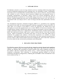
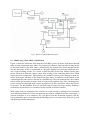
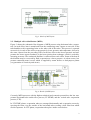
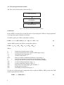
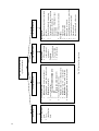
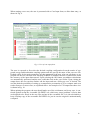
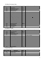
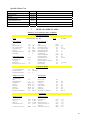
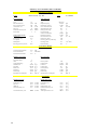
CO MPU T ER M A N UAL S E RI E S No . 1 9
Desalination Economic
Evaluation Program
(DEEP-3.0)
User’s Manual
COMPUTER MANUAL SERIES No. 19
Desalination Economic
Evaluation Program
(DEEP-3.0)
User’s Manual
INTERNATIONAL ATOMIC ENERGY AGENCY, VIENNA, 2006
The originating Section of this publication in the IAEA was:
Nuclear Power Technology Development Section
International Atomic Energy Agency
Wagramer Strasse 5
P.O. Box 100
A-1400 Vienna, Austria
DESALINATION ECONOMIC EVALUATION PROGRAM
(DEEP-3.0)
IAEA, VIENNA, 2006
IAEA-CMS-19
© IAEA, 2006
Printed by the IAEA in Austria
April 2006
FOREWORD
DEEP is a Desalination Economic Evaluation Program developed by the International
Atomic Energy Agency (IAEA) and made freely available for download, under a license
agreement (www.iaea.org/nucleardesalination). The program is based on linked Microsoft
Excel spreadsheets and can be useful for evaluating desalination strategies by calculating
estimates of technical performance and costs for various alternative energy and desalination
technology configurations. Desalination technology options modeled, include multi-stage
flashing (MSF), multi-effect distillation (MED), reverse osmosis (RO) and hybrid options
(RO-MSF, RO-MED) while energy source options include nuclear, fossil, renewables and
grid electricity (stand-alone RO) .
Version 3 of DEEP (DEEP 3.0) features important changes from previous versions,
including upgrades in thermal and membrane performance and costing models, the
coupling configuration matrix and the user interface. Changes in the thermal performance
model include a revision of the gain output ratio (GOR) calculation and its generalization to
include thermal vapour compression effects. Since energy costs continue to represent an
important fraction of seawater desalination costs, the lost shaft work model has been
generalized to properly account for both backpressure and extraction systems. For RO
systems, changes include improved modeling of system recovery, feed pressure and
permeate salinity, taking into account temperature, feed salinity and fouling correction
factors. The upgrade to the coupling technology configuration matrix includes a recategorization of the energy sources to follow turbine design (steam vs. gas) and cogeneration features (dual-purpose vs. heat-only). In addition, cost data has also been
updated to reflect current practice and the user interface has been refurbished and made
user-friendlier.
The IAEA officers responsible for this publication were M. Methnani and B. Misra of the
Division of Nuclear Power.
EDITORIAL NOTE
The use of particular designations of countries or territories does not imply any judgement by the
publisher, the IAEA, as to the legal status of such countries or territories, of their authorities and
institutions or of the delimitation of their boundaries.
The mention of names of specific companies or products (whether or not indicated as registered) does
not imply any intention to infringe proprietary rights, nor should it be construed as an endorsement
or recommendation on the part of the IAEA.
CONTENTS
1.
INTRODUCTION....................................................................................................................... 1
2.
DESALINATION PROCESSES ................................................................................................ 1
2.1. Multi stage flash (MSF) distillation...................................................................................... 2
2.2. Multiple effect distillation (MED)........................................................................................ 3
2.3. MED plants with vapour compression (VC) ........................................................................ 4
2.4. Reverse osmosis (RO) .......................................................................................................... 4
3.
DEEP-3.0 PROGRAM CHANGES ............................................................................................ 4
4.
DEEP-3.0 MODEL DESCRIPTION........................................................................................... 5
4.1. Thermal performance model................................................................................................. 6
4.2. RO performance model......................................................................................................... 8
4.3. Hybrid performance model................................................................................................... 9
4.4. Cost model............................................................................................................................ 9
5.
DEEP-3.0 PROGRAM INSTRUCTIONS ................................................................................ 10
5.1. Installing DEEP .................................................................................................................. 10
5.2. Running a DEEP case......................................................................................................... 10
5.3. Case input form .................................................................................................................. 11
6.
DEEP-3.0 INPUT OUTPUT DESCRIPTION .......................................................................... 14
6.1. Input sheet........................................................................................................................... 14
6.2. Output sheet........................................................................................................................ 18
7.
DEEP-3.0 SAMPLE CASES .................................................................................................... 19
REFERENCES.................................................................................................................................. 23
CONTRIBUTORS TO DRAFTING AND REVIEW....................................................................... 25
1. INTRODUCTION
Desalination is known to be an energy intensive process, requiring mainly low-temperature
steam for distillation and high-pressure pumping power for membrane systems. Traditionally,
fossil fuels such as oil and gas have been the major energy sources. However, fuel price hikes
and volatility as well as concerns about long-term supplies and environmental release is
prompting consideration of alternative energy sources for sewater desalination, such as
nuclear desalination [1] and the use of renewable energy sources[2]. If we add to this the fact
that the coupling methods between power and desalination units can also vary, the need for a
performance and cost analysis tool to assist in design selection and optimization becomes
clear.
The Desalination Economic Evaluation Program (DEEP) is a spreadsheet tool originally
developed for the IAEA by General Atomics[3] and later expanded in scope by the IAEA, in
what came to be known as the DEEP-2 version [4]. Recently, the models have been
thoroughly reviewed and upgraded and a new version, DEEP-3.0, has been released[5]. The
program allows designers and decision makers to compare performance and cost estimates of
various desalination and power configurations. Desalination options modeled include MSF,
MED, RO and hybrid systems while power options include nuclear, fossil and renewable
sources. Both co-generation of electricity and water as well as water-only plants can be
modeled. The program also enables a side-by-side comparison of a number of design
alternatives, which helps identify the lowest cost options for water and power production at a
specific location. Data needed include the desired configuration, power and water capacities
as well as values for the various basic performance and costing data.
2. DESALINATION PROCESSES
Desalination systems fall into two main design categories, namely thermal and membrane
types [6]. Thermal designs including multi-stage flash (MSF) and Multi-effect distillation
(MED), use flashing and evaporation to produce potable water while membrane designs use
the method of Reverse Osmosis (RO), shown in Fig. 1. With continuing improvements in
membrane performance, RO technology is increasingly gaining markets in seawater
desalination and hybrid configurations, combining RO with MED or RO with MSF have also
been considered (Fig. 2.).
Fig. 1. Sketch of RO layout.
1
Fig. 2. Sketch of hybrid MED-RO layout.
2.1. Multi stage flash (MSF) distillation
Figure 2 shows the schematic flow diagram of an MSF system. Seawater feed passes through
tubes in each evaporation stage where it is progressively heated. Final seawater heating occurs
in the brine heater by the heat source. Subsequently, the heated brine flows through nozzles
into the first stage, which is maintained at a pressure slightly lower than the saturation pressure of the incoming stream. As a result, a small fraction of the brine flashes forming pure
steam. The heat to flash the vapour comes from cooling of the remaining brine flow, which
lowers the brine temperature. Subsequently, the produced vapour passes through a mesh demister in the upper chamber of the evaporation stage where it condenses on the outside of the
condensing brine tubes and is collected in a distillate tray. The heat transferred by the condensation warms the incoming seawater feed as it passes through that stage. The remaining brine
passes successively through all the stages at progressively lower pressures, where the process
is repeated. The hot distillate flows as well from stage to stage and cools itself by flashing a
portion into steam which is re-condensed on the outside of the tube bundles.
MSF plants need pre-treatment of the seawater to avoid scaling by adding acid or advanced
scale-inhibiting chemicals. If low cost materials are used for construction of the evaporators, a
separate deaerator is to be installed. The vent gases from the deaeration together with any
non-condensable gases released during the flashing process are removed by steam-jet ejectors
and discharged to the atmosphere.
2
2
Fig. 3. Sketch of MSF layout.
2.2. Multiple effect distillation (MED)
Figure 3 shows the schematic flow diagram of MED process using horizontal tube evaporators. In each effect, heat is transferred from the condensing water vapour on one side of the
tube bundles to the evaporating brine on the other side of the tubes. This process is repeated
successively in each of the effects at progressively lower pressure and temperature, driven by
the water vapour from the preceding effect. In the last effect at the lowest pressure and temperature the water vapour condenses in the heat rejection heat exchanger, which is cooled by
incoming seawater. The condensed distillate is collected from each effect. Some of the heat in
the distillate may be recovered by flash evaporation to a lower pressure. As a heat source, low
pressure saturated steam is used, which is supplied by steam boilers or dual-purpose plants
(co-generation of electricity and steam).
Fig. 4. Sketch of MED layout.
Currently, MED processes with the highest technical and economic potential are the low temperature horizontal tube multi-effect process (LT-HTME) and the vertical tube evaporation
process (VTE).
In LT-HTME plants, evaporation tubes are arranged horizontally and evaporation occurs by
spraying the brine over the outside of the horizontal tubes creating a thin film from which
steam evaporates. In VTE plants, evaporation takes place inside vertical tubes.
3
2.3. MED plants with vapour compression (VC)
In some MED designs, a part of the vapour produced in the last effect is compressed to a
higher temperature level so that the energy efficiency of the MED plant can be improved (vapour compression). To compress the vapour, either mechanical or thermal compressors are
used.
2.4. Reverse osmosis (RO)
Reverse osmosis is a membrane separation process in which pure water is “forced” out of a
concentrated saline solution by flowing through a membrane at a high static transmembrane
pressure difference. This pressure difference must be higher than the osmotic pressure between the solution and the pure water. The saline feed is pumped into a closed vessel where it
is pressurised against the membrane. As a portion of the water passes through the membrane,
the salt content in the remaining brine increases. At the same time, a portion of this brine is
discharged without passing through the membrane.
RO membranes are made in a variety of modular configurations. Two of the commercially
successful configurations are spiral-wound modules and hollow fibre modules. The membrane performance of RO modules such as salt rejection, permeate product flow and membrane compaction resistance were improved tremendously in the last years. The DEEP performance models cover both the effect of seawater salinity and the effect of seawater temperature on recovery ratio and required feedwater pressure.
A key criterion for the RO layout is the specific electricity consumption, which should be as
low as possible. That means, the recovery ratio has to be kept as high as possible and the accompanying feedwater pressure as low as possible fulfilling the drinking water standards as
well as the design guidelines of the manufactures. Since the overall recovery ratios of current
seawater RO plants are only 30 to 50%, and since the pressure of the discharge brine is only
slightly less than the feed stream pressure, all large-scale seawater RO plants as well as many
smaller plants are equipped with energy recovery turbines.
3. DEEP-3.0 PROGRAM CHANGES
Version three features important changes from previous versions, including upgrades in
thermal and membrane performance and costing models, the coupling configuration matrix
and the user interface, as well as a thorough review of the configuration templates.
•
The thermal model upgrade includes:
1. A generalization of the lost shaft work to model both extraction and
backpressure coupling configurations.
2. Improvements in the distillation thermal balance model and Gain
Output Ratio (GOR) calculation.
3. Adding a new Thermal Vapor Compression (TVC) option.
4
4
•
The RO model, upgrade includes:
1. New and validated correlations for feed pressure and permeate
salinity, accounting for the effects of feed salinity, temperature and
fouling.
2. A new correlation for recovery ratio estimates.
•
The coupling configuration upgrade includes a re-categorization of the energy
sources to follow current practice. The coupling scheme selection follows turbine
design (steam vs. gas) and co-generation features (dual-purpose vs. heat-only). The
energy source categorization includes nuclear, fossil and renewable options, with the
latter being a new addition.
4. DEEP-3.0 MODEL DESCRIPTION
A flow chart for the overall programme layout is shown in Fig. 5.
Input Forms/Sheets
Performance Analysis
Thermal/RO
Cost Anlaysis
Thermal/RO
Output Sheets
Fig. 5. General DEEP program layout.
This section gives a brief overview of the models, including the thermal and RO performance
models as well as the costing model.
5
4.1. Thermal performance model
The flow chart for this model is shown in Fig. 6.
GOR Calculation
Flow/Pumping Power
Calculations
Lost Shaft Work
Fig. 6. Flowchart for thermal performance model.
GOR Model
In the DEEP-3.0 model, the user has the choice of specifying the GOR as a design parameter
or letting the program calculate an estimate.
For MSF systems, the GOR is calculated as follows:
GOR = λh / ch / (dTbh +dTbpe)* ( 1 - exp( -cvm * dTao / λm )
(1)
And for MED systems, the GOR is calculated as follows:
GOR = λh / (λm * dTae / dTdo + ch * ( dTph + dTbpe ) )
(2)
Where
λh
λm
Tmb
Tsw
DTdls
ch
cvm
dTao
dTae
dTbh
dtbpe
dTph
=
=
=
=
=
latent heat of heating vapour, kJ/kg
average latent heat of water vapour in MSF stages, kJ/kg
maximum brine temperature, °C
seawater temperature, °C
brine to seawater temperature difference in last stage, °C
specific heat capacity of feedwater in brine heater, kJ/kg/K
average specific heat capacity of brine in MSF plant, kJ/kg/K
overall working temperature range, °C
average temperature drop per effect, °C
brine heater feed temperature gain for MSF, °C
boiling point elevation, °C
Preheating feed temperature gain, °C
For the case of thermal vapor compression units coupled to MED or MSF systems, the GOR
model is generalized as follows:
GORtvc = GOR(1+Rtvc)
6
(3)
Where Rtvc is defined as the ratio of entrained vapour flow to motive steam flow, an input design parameter.
The top brine temperature Tmb is also retained as a design parameter and as such, can be input
by the user or alternatively, calculated given an input steam temperature.
Given as input the salt concentration factor CF, the cooling seawater temperature gain ΔTc
and the product water flow rateWp, estimates for reject brine flow Wb , make-up feed flow Wf
and condenser cooling water flow Wc, could also be calculated as follows,
Wb = Wp / (CF-1)
Wf = CF.Wb
Wc= Qc / (ccΔTc)
(4)
(5)
(6)
Where Qc refers to the net condenser heat load and cc refers to the specific heat capacity of
cooling water.
While specific heat transfer areas could also be calculated in DEEP in a straightforward manner, the current approach, where user input is expected for specific capital costs ($/m3/d), is
considered adequate for the purposes of DEEP and is therefore retained.
Lost Shaft Work Model
In DEEP-3.0, the lost shaft work is calculated as follows (except for the heat-only case,
where it is set to zero, as follows:
For the backpressure case,
Qls = (Qst /(1-η)).η
(7)
With Qst = Qcr
Where Qcr refers to the condenser heat load,
η =ηlpt .(Tcm-Tc)/(Tcm + 273)
(8)
ηlpt refers to low pressure turbine isentropic efficiency, and
Tc and Tcm refer to the condenser reference and modified temperatures in °C.
For the extraction case,
Qls = Qst.η
(9)
With Qst = Wst.hfg
Where hfg is the steam latent heat, assuming saturation conditions.
and η is redefined as,
η =ηlpt .(Tst-Tc)/(Tst + 273)
(10)
7
Where Tst = Textracted steam in °C
Note that the cases involving available waste heat, such as gas cooled reactors correspond to a
backpressure configuration with
And
Tcm = Tc
Qls = 0
Which implies free available heat and no lost shaft work.
For the backup pressure cases, the heating steam is limited by the heat exchanger or condenser load. For extraction cases, it is limited by the available heat source. The following expression is used:
Qst
< (Qt – Qe)/(1-η)
(11)
Where Qt refers to the available thermal power and Qe refers to the produced electric power.
4.2. RO performance model
The flow chart for the Reverse Osmosis (RO) model is shown in Fig. 7:
Recovery ration Estimate
Product Flow & Quality Estimate
Feed Flow & Pressure Estimate
Pumping Power Requirements
Fig. 7. Flowchart for RO performance model.
Here, again, the user can either specify the system recovery ratio, or have it estimated by
DEEP, as follows:
R = 1 – CNS . Sf
(12)
Where
Sf refers to the feed salinity in ppm and C is a constant defined as
CNS = 1.15E-3/Pmax
Pmax refers to the maximum design pressure of the membrane in bars.
8
(13)
8
Note that as feed salinity becomes small, the recovery ratio approaches unity and as it approaches the numerical equivalent of maximum membrane pressure (in millibars), recovery
goes to zero, as would be expected in practice.
For permeate salinity and feed pressure, we use the expressions given by Wilf [7], which take
into account feed temperature and salinity correction factors and have been verified against
commercial design data.
Feed pressure Pf is calculated as follows:
Pf = ∆pd + Posm + ∆pl
(14)
Where
∆pd = φd / φn. ∆pn.ct.cs.cf
(15)
And
Posm is the average osmotic pressure across the system;
∆pl is the corresponding pressure loss;
∆pd and φd are the design net driving pressure and flux;
∆pn and φn are the nominal net driving pressure and flux; and
ct, cs and cf are correction factors related to temperature, salinity and fouling.
Permeate salinity Sp on the other hand, is calculated as follows:
Where
Sp = (1-rm). Sf. φn / φd. c΄r. c΄t
(16)
Sf refers to feed salinity; and
c΄r and c΄t are correction factors related to recovery and temperature.
rm refers to the membrane salt reject fraction.
For the calculation of energy recovery Qer, given the energy recovery efficiency ξer , both
Pelton-type and work exchanger designs are modeled as follows:
For the Pelton design,
Qer = (1-rm) . ξer Qhp
(17)
Where Qhp refers to the available high pumping power, adjusted for system losses.
4.3. Hybrid performance model
Hybrid methods refer to the use of a combined configuration, usually an RO + MED or an RO
+ MSF configuration. These configurations have been designed with an eye on improving
product water quality and operational flexibility [8] and DEEP allows their simulation,
through a combination of the thermal and RO models described above.
4.4. Cost model
Cost calculations in DEEP are done for both power and water plants and are case-sepcific.
Capital costs as well as fuel, operation and maintenance and other costs are taken into consideration. Water capacity scaling is taken into account in cost calculations if specified by the
user.
9
9
DEEP uses the power credit method [9] to estimate the value of steam in co-generation systems. The essence of this method is that the cost of the low-pressure steam Cst per unit volume of produced water is determined by the lost value of the additional electric power ΔQe,
(KWh), which could have been produced instead. This is sometimes alternatively referred to
as the lost shaft work.
Cst = Ce . ΔQe/Wp
(18)
Where Ce is the base electricity cost per KWh and Wp is the volumetric water production rate
per hour. While there are other methods available, for high power-to-water ratios, the power
credit method is considered adequate.
5. DEEP-3.0 PROGRAM INSTRUCTIONS
The DEEP programme structure is based on the linking of macro-enabled Excel spreadsheets.
The linking procedure enables the separation of the calculation and presentation parts of the
software.
Performance and cost estimates of co-generated electricity and water, or alternatively, water
for water-only plants, are calculated by the programme engine, DEEP.xls and saved in separate case files under the “User Files/Cases” subfolder. In the process, the programme makes
use of pre-composed configuration templates (subfolder templates). DEEP also includes features allowing a comparative result presentation of up to nine pre-run cases and results are
saved under the “User Files/CPs” subfolder.
5.1. Installing DEEP
The installation of DEEP has been tested under Windows 2000 and Windows XP. A minimum free disk size of of 11 Mbytes is needed, including about 3 MB for the executable file
“DEEP3.xls” and 7 MB for the template folder. The user should make sure that the DEEP3
folder is not write-protected and that the Excel security level is not set to “high”, in order to
enable macros.
5.2. Running a DEEP case
The programme is executed by double-clicking on the DEEP3.xls icon in the root folder. At
startup, the user is prompted to enable macros and is presented with the main program window. Options available to the user include the following options:
New case
This option is selected to start a new case. A Case Input Form is presented for input of the main case parameters.
View case
This option is selected to load an existing case file.
10
Edit input data
This option is selected to edit input for an active case. All data can
be edited, with the exception of the configuration options, which can
only be changed from the Case Input Form. Double-clicking on any
cell marked in green, allows the user to modify its content.
Show case results
This option is selected to show results for an active case. The output
summary includes main case parameters and configuration options
as well as performance and cost results. It can be printed on a single
sheet.
New/edit CP
This option is selected to start a new Comparative Presentation (CP)
case, for side-to-side comparison of existing cases. The user may be
prompted to update reference links to the "CPnull" template located
in the DEEP-3.0 root directory and is then prompted to specify the
name of the CP save file and to select the cases to be compared.
View CP
This option is selected to load an existing CP presentation file.
Show CP results
This option is selected to show contents of an active CP presentation.
View directories
This option is selected to view the DEEP-3.0 directory structure.
5.3. Case input form
The flowchart for input data is shown in Fig. 8.
11
12
1. Configuration type:
1. Dual (power & water) (extraction vs.
backpressure – waste heat – shared costs)
2. Dedicated (water only)
2. Type of water plant:
1.
Thermal: MED/MSF/MED-TVC
2.
RO
3.
Hybrid (RO-MED/RO-MSF)
3. Type of thermal energy source:
3. Nuclear (steam cycle vs Brayton cycle)
4. Fossil (oil – gas – CC – coal -diesel) –
5. Renewable (solar – wind – biomass)
4. Coupling scheme: Intermediate loop data
1. User & project
data
2. Case
identification
data
Design data:
• Power capacity &
other relevant
parameters
Cost data:
1. Capital cost data
2. Fuel cost data
3. O&M cost data
Power plant data
Fig. 8. Flowchart for input data.
Configuration data
Project data
User input forms & function
specific worksheets
Design data:
1. Required water capacity or available
heat data
2. Water feed salinity & temperature
3. For thermal cases: Steam or top brine
temperatures - Number of
effects/stages – Entrainment vapor
ratio for TVC
4. For RO: energy recovery fraction
Cost data:
1. Capital cost data
2. O&M cost data
3. Backup power cost data
4. Amortization data (interest – plant life)
5. Levelized electricity cost data
6. Shared cost data
7. Intermediate loop & other costs
Water plant data
When starting a new case, the user is presented with a Case Input form, to allow data entry, as
shown in Fig. 9.
Fig. 9. View of case input form.
The user is expected to first select the desired coupling configuration from the matrix of supported energy and desalination coupling options and also specify the name of the case save file.
Default values for the main parameters are then presented to the user, who can edit them, as approprate for the case. Because error checking in DEEP is minimal, the user is cautioned to check
the accuracy of the input data entered. Upon selecting the OK button, spreadsheet calculations
are automatically performed and the user could then look at the case results. Upon closing the
output sheet, the user can then further edit the input and run a follow up case, if desired. The
user has then the possibility of setting up a comparative presentation (CP), to compare main cost
results from two or more cases, as explained above. An example of a CP comparison sheet view
is shown in Fig. 10.
When quitting the program, the user should make use of the exit button, and in any case, is cautioned against saving the executable file DEEP3.xls, which may cause problems. All user data
are designed to be stored in the case files and not in the executable file. It is also adviasable to
keep a backup copy of the executable file DEEP3.xls, just in case the original is unintentionally
corrupted.
13
Wa te r Co st
1.000
0.900
0.800
0.700
$ / m3
0.600
0.500
0.400
0.300
0.200
0.100
0.000
CC+MED-RO-$15-
CC+MED-RO-15$-
5%
10%
CC+MED-RO-30$
CC+MED-RO-50$
Nuclear Gas
NGT+MED-RO-10%
Turbine+MED-RO-5%
CC+MED-RO-$15+MED-RO-15$-1C+MED-RO-30C+MED-RO-50as Turbine +ME
GT+MED-RO-10
Wa te r cos t
0.614
0.614
0.737
0.902
0.545
0.553
Unit
$ / m3
Fig. 10. View of a comparative DEEP-3.0 presentation.
6. DEEP-3.0 INPUT OUTPUT DESCRIPTION
6.1. Input sheet
Case Identification & Basic Configuration
Input Variable
Project
Unit
Project identification
text
Case
Case identification
text
EnPlt
Energy plant type
text
Desalination plant type
text
DslpType
RefDiag
14
Description
Reference coupling diagram
Default
Remarks
#
14
Energy Plant Performance Data
Input Variable
Description
Unit
Qtp
Ref. thermal power
MWt
Pen
Ref. net electric power
Mwe
opp
Planned outage rate
oup
Unplanned outage rate
Appo
if 0, value is calculated
Operating availability
kec
Energy plant contingency factor
Le
Construction lead time
m
Tair
Site specific inlet air temp
Condenser-to-Interm. loop approach
temp.
°C
DTft
a
0
28
for GT/CC cases
Default
Remarks
°C
Turbine type (ExtrCon / BackPr)
DT1s
Interm. loop temperature drop
Difference between feed steam temp.
and max brine temp.
°C
DPip
Intermediate loop pressure loss
bar
Eip
600 or 0 (RH,NH,FH)
0,110
Lifetime of energy plant
TurType
Remarks
0,100
Lep
DTca
Default
°C
Intermediate loop pump efficiency
Energy Plant Cost Data
Input Variable
Ce
Ceom
Description
Specific construction cost
Specific O&M cost
eff
Fossil fuel annual real escalation
Cff
Specific fossil / renewable fuel cost
Cnsf
ir
Specific nuclear fuel cost
Interest rate
Ycr
Currency reference year
Ycd
Initial construction date
Yi
Initial year of operation
Lwp
Lifetime of water plant
LBKo
cpe
kdcopp
Lifetime of backup heat source
Purchased electricity cost
Decommissioning cost
Unit
$/KW
$/MW(e).h
%/a
$/ton or
OE
2
$/MWh
%
a
a
$/Kwe
% of Ce
30
for nuclear cases
15
Distillation Plant Performance Data
Input Variable
Description
Wc_t
Required capacity
Tsdo
Seawater feed temp
TDS
Feed salinity
Unit
Default
m3/d
100000
°C
if 0, value is calculated
GOR
Wduo
Distillation plant modular unit size
DTdcr
Condenser range
°C
DTdca
Condenser approach
°C
Tcmo
Steam temperature
oC
Tmbo
Max. brine temperature
°C
TVC
Thermal vapor compression option
Y/N
Rtvco
TVC vapor entrainment ratio
Esd
Qsdp
Seawater pump head
m3/d
Specific power use
Planned outage rate
oud
Unplanned outage rate
bar
Backup heat source option flag
opb
Backup heat planned outage rate
oub
Backup heat unplanned outage rate
10
5
if 0, value is calculated
if 0, value is calculated
1,7
0,85
kW(e)h/m3
0,030
0,065
if 0, value is calculated
Plant availability
BK
0
1
Seawater pump efficiency
opd
Adpo
30
ppm
GORo
DPsd
Remarks
Y/N
Distillation Plant Cost Data
Input Variable
Wdur
Cdu
Plant base unit cost
Csdo
Infall/outfall cost
Cil
Intermediate loop cost
kdc
Plant cost contingency factor
kdo
Plant owners cost factor
Unit
3
$/(m /d)
0,05
Average management salary
$/a
Average labor salary
$/a
csds
Specific O&M spare parts cost
$/m3
cdtr
Tubing replacement cost
Specific O&M chemicals cost for pretreatment
Specific O&M chemicals cost for posttreatment
$/m3
Cbuo
Cffb
effb
Ndmo
Ndlo
Plant O&M insurance cost
Backup heat source unit cost
Fossil fuel price for backup heat source
at startup
Fossil fuel real escala. for backup heat
source
Num. of management personnel
Number of labor personnel
0
0,1
Sdm
kdi
% of construction cost
%
m
cdcpo
Remarks
$/(m3/d)
Plant construction lead time
cdcpr
Default
m3/d
Ldo
Sdl
16
Description
Reference modular unit size for cost
adjustment
$/m3
%
$/MW(t)
if 0, value is calculated
66000
29700
0,03
0,03
0,02
0,5
55000
20
$/bbl
2
%/a
if 0, value is calculated
0
16
RO Plant Performance Data
Input Variable
Wct
Description
Required capacity
Unit
RO feedwater inlet temperature
Wmuo
RO plant modular unit size
m3/d
DPsm
Seawater pump head
bar
Seawater pump efficiency
TDS
Feed salinity
Rro
Recovery ratio
Dflux
Eer
EerType
DPbm
Ebm
DPhm
°C
30
ppm
Design flux
l/(m2.h)
Energy recovery efficiency
PLT / PEX
RO energy recovery device type
Booster pump head
bar
Booster pump efficiency
High head pump pressure rise
Ehm
High head pump efficiency
Ehhm
Hydraulic pump coupling efficiency
Qsom
Other specific power use
opm
Planned outage rate
oum
Unplanned outage rate
Ampo
Remarks
m3/d
Tsmo
Esm
Default
bar
kW(e)h/m3
if 0, value is calculated
Plant availability
RO Plant Cost Data
Input Variable
Description
Cmu
RO plant base unit cost
Csmo
Infall/outfall cost
Unit
kmo
Plant owners cost factor
Lmo
Plant availability
Smm
Average management salary
$/a
Sml
Average labor salary
$/a
cmm
O&M membrane replacement cost
$/m3
cmsp
O&M spare parts cost
$/m3
cmcpr
Specific chemicals cost for pre-treatment
$/m3
cmcpo
Specific chemicals cost for post-treatment
$/m3
Nmmo
Num. of management personnel
Nmlo
Number of labor personnel
Lho
Hybrid plant lead time
% of construction cost
%
Plant cost contingency factor
Plant O&M insurance cost
Remarks
$/(m /d)
kmc
kmi
Default
3
if 0, value is calculated
%
if 0, value is calculated
m
if 0, value is calculated
Hybrid Plant Data
Input Variable
Description
Unit
Required total desalination capacity
m3/d
Wc_dst
Hybrid dist. capacity
m3/d
Wc_RO
Hybrid RO capacity
m3/d
Wc_t
Lho
Hybrid plant lead time
m
Default
Remarks
0
17
6.2. Output sheet
Performance Results
Description
Lost Electricity Production
Power-to-Heat Ratio
Plant Thermal Utilization
Unit
Remarks
MW
MWe/MWt
%
Distillation Performance
Description
# of Effects/Stages
GOR
Unit
Remarks
MW
MWe/MWt
Temperature Range
°C
Distillate Flow
m3/d
Feed Flow
m3/d
Steam Flow
kg / s
Brine Flow
m3/d
Brine salinity
ppm
Specific Heat Consumption
kWh / m3
RO Performance
Description
Unit
Recovery Ratio
MW
Permeate Flow
m3/d
Feed Flow
m3/d
Feed Pressure
bar
Product Quality
ppm
Brine Flow
m3/d
Brine salinity
ppm
Specific Power Consumption
Remarks
kWh / m3
Cost results
Specific Power Cost
Description
Unit
Fixed charge cost
$ / kWh
Fuel cost
$ / kWh
O&M cost
$ / kWh
Decommissioning cost
$ / kWh
Levelized Electricity Cost
$ / kWh
18
Remarks
18
Specific Water Cost
Description
Remarks
Unit
Fixed charge cost
$ / m3
Heat cost
$ / m3
Plant electricity cost
$ / m3
Purchased electricity cost
$ / m3
O&M cost
$ / m3
Total Specific Water Cost
$ / m3
7.
DEEP-3.0 SAMPLE CASES
Summary of Performance and Cost Results
Main Input Parameters
Project
DEEP Version 3.0 - Sep. 2005
Power Plant Data
Type
Ref. Thermal Power
Ref. Net Electric Power
Construction Cost
Fuel Cost
Purchased Electricity Cost
Interest Rate
Configuration Switches
Steam Source
Intermediate Loop
TVC Option
Backup Heat
RO Energy Recovery Device
Case
CC+MED
Water Plant Data
CC
1,200
600
700
50
0.037
5
Type
Required capacity
Hybrid Dist. Capacity
Dist. Construction Cost
Maximum Brine Temp.
Heating Steam Temp.
Dist. Feed Temp.
Seawater Feed Salinity
Hybrid RO Capacity
RO Construction Cost
RO Recovery Ratio
RO Energy Recovery Efficiency
RO Design Flux
RO Feed Temp.
MW
MW
$ / kW
$/BOE
$/kWh
%
ExtrCon
N/A
N
N
N/A
MED
100,000
N/A
900
65.0
0.0
30
35000.0
N/A
N/A
N/A
N/A
N/A
N/A
m3/d
m3/d
$ / (m3/d)
°C
°C
°C
ppm
m3/d
$ / (m3/d)
l / (m2 hour)
°C
Performance Results
Lost Electricity Production
Power-to-Heat Ratio
Plant Thermal Utilization
20.0
1.7
75.5
MW
MWe/MWt
%
Distillation Performance
# of Effects/Stages
GOR
Temperature Range
Distillate Flow
Feed Flow
Steam Flow
Brine Flow
Brine salinity
Specific Heat Consumption
RO Performance
9
8.0
20
100,000
200,000
144.39
100,000
70,000
80.67
°C
3
m /d
3
m /d
kg / s
3
m /d
ppm
3
kWh / m
Recovery Ratio
Permeate Flow
Feed Flow
Feed Pressure
Product Quality
Brine Flow
Brine Saliniy
Specific Power Consumption
N/A
N/A
N/A
N/A
N/A
N/A
N/A
N/A
m /d
3
m /d
bar
ppm
3
m /d
ppm
3
kWh / m
0.328
0.424
0.204
0.000
0.139
1.093
$/m
3
$/m
3
$/m
3
$/m
3
$/m
3
$/m
3
Cost Results
Specific Power Costs
Specific Water Costs
Fixed charge cost
Fuel cost
O&M cost
Decommissioning cost
0.008
0.075
0.006
N/A
$ / kWh
$ / kWh
$ / kWh
$ / kWh
Levelized Electricity Cost
0.088
$ / kWh
Fixed charge cost
Heat cost
Plant electricity cost
Purchased electricity cost
O&M cost
Total Specific Water Cost
3
19 19
Summary of Performance and Cost Results
Main Input Parameters
Project
DEEP Version 3.0 - Sep. 2005
Power Plant Data
Type
Ref. Thermal Power
Ref. Net Electric Power
Construction Cost
Fuel Cost
Purchased Electricity Cost
Interest Rate
Configuration Switches
Steam Source
Intermediate Loop
TVC Option
Backup Heat
RO Energy Recovery Device
Case
CC+MED-RO
Water Plant Data
CC
1,200
600
700
50
0.037
5
Type
Required capacity
Hybrid Dist. Capacity
Dist. Construction Cost
Maximum Brine Temp.
Heating Steam Temp.
Dist. Feed Temp.
Seawater Feed Salinity
Hybrid RO Capacity
RO Construction Cost
RO Recovery Ratio
RO Energy Recovery Efficiency
RO Design Flux
RO Feed Temp.
MW
MW
$ / kW
$/BOE
$/kWh
%
ExtrCon
N/A
N
N
PEX
MED-RO
100,000
50,000
900
65.0
0.0
30
35000.0
50,000
900
0.00
0.95
13.6
30.0
m3/d
m3/d
$ / (m3/d)
°C
°C
°C
ppm
m3/d
$ / (m3/d)
l / (m2 hour)
°C
Performance Results
Lost Electricity Production
Power-to-Heat Ratio
Plant Thermal Utilization
10.0
3.5
62.8
MW
MWe/MWt
%
RO Performance
Distillation Performance
# of Effects/Stages
GOR
Temperature Range
Distillate Flow
Feed Flow
Steam Flow
Brine Flow
Brine salinity
Specific Heat Consumption
9
8.0
20
50,000
100,000
72.20
50,000
70,000
80.67
°C
m3/d
m3/d
kg / s
m3/d
ppm
kWh / m3
Recovery Ratio
Permeate Flow
Feed Flow
Feed Pressure
Product Quality
Brine Flow
Brine Saliniy
Specific Power Consumption
0.42
50,000
120,000
56.1
279
70,000
60,000
2.91
m3/d
m3/d
bar
ppm
m3/d
ppm
kWh / m3
Cost Results
Specific Power Costs
20
Specific Water Costs
Fixed charge cost
Fuel cost
O&M cost
Decommissioning cost
0.008
0.075
0.006
N/A
$ / kWh
$ / kWh
$ / kWh
$ / kWh
Levelized Electricity Cost
0.088
$ / kWh
Fixed charge cost
Heat cost
Plant electricity cost
Purchased electricity cost
O&M cost
Total Specific Water Cost
0.301
0.195
0.213
0.007
0.158
0.873
$ / m3
$ / m3
$ / m3
$ / m3
$ / m3
$ / m3
20
Summary of Performance and Cost Results
Main Input Parameters
Project
DEEP Version 3.0 - Sep. 2005
Power Plant Data
Type
Ref. Thermal Power
Ref. Net Electric Power
Construction Cost
Fuel Cost
Purchased Electricity Cost
Interest Rate
Configuration Switches
Steam Source
Intermediate Loop
TVC Option
Backup Heat
RO Energy Recovery Device
Case
NBC+MED-RO
Water Plant Data
NBC
1,570
660
1,500
6
0.06
5
Type
Required capacity
Hybrid Dist. Capacity
Dist. Construction Cost
Maximum Brine Temp.
Heating Steam Temp.
Dist. Feed Temp.
Seawater Feed Salinity
Hybrid RO Capacity
RO Construction Cost
RO Recovery Ratio
RO Energy Recovery Efficiency
RO Design Flux
RO Feed Temp.
MW
MW
$ / kW
$/MWh
$/kWh
%
ExtrCon
Y
N
N
PEX
MED-RO
100,000
50,000
900
65.0
0.0
30
35000.0
50,000
900
0.00
0.95
13.6
30.0
m3/d
m3/d
$ / (m3/d)
°C
°C
°C
ppm
m3/d
$ / (m3/d)
l / (m2 hour)
°C
Performance Results
Lost Electricity Production
Power-to-Heat Ratio
Plant Thermal Utilization
0.0
3.9
52.4
MW
MWe/MWt
%
Distillation Performance
# of Effects/Stages
GOR
Temperature Range
Distillate Flow
Feed Flow
Steam Flow
Brine Flow
Brine salinity
Specific Heat Consumption
RO Performance
9
8.0
20
50,000
100,000
72.20
50,000
70,000
80.67
°C
m3/d
m3/d
kg / s
m3/d
ppm
kWh / m3
Recovery Ratio
Permeate Flow
Feed Flow
Feed Pressure
Product Quality
Brine Flow
Brine Saliniy
Specific Power Consumption
0.42
50,000
120,000
56.1
279
70,000
60,000
2.91
m3/d
m3/d
bar
ppm
m3/d
ppm
kWh / m3
Cost Results
Specific Power Costs
Specific Water Costs
Fixed charge cost
Fuel cost
O&M cost
Decommissioning cost
0.013
0.009
0.012
0.004
$ / kWh
$ / kWh
$ / kWh
$ / kWh
Levelized Electricity Cost
0.037
$ / kWh
Fixed charge cost
Heat cost
Plant electricity cost
Purchased electricity cost
O&M cost
Total Specific Water Cost
0.311
0.000
0.097
0.006
0.157
0.571
$ / m3
$ / m3
$ / m3
$ / m3
$ / m3
$ / m3
21 21
Summary of Performance and Cost Results
Main Input Parameters
Project
DEEP Version 3.0 - Sep. 2005
Power Plant Data
Case
Stand-Alone RO
Water Plant Data
Type
Ref. Thermal Power
Ref. Net Electric Power
Construction Cost
Fuel Cost
Purchased Electricity Cost
Interest Rate
N/A
N/A
N/A
N/A
N/A
0.037
5
Configuration Switches
Steam Source
Intermediate Loop
TVC Option
Backup Heat
RO Energy Recovery Device
N/A
Y
N/A
N/A
PEX
Type
Required capacity
Hybrid Dist. Capacity
Dist. Construction Cost
Maximum Brine Temp.
Heating Steam Temp.
Dist. Feed Temp.
Seawater Feed Salinity
Hybrid RO Capacity
RO Construction Cost
RO Recovery Ratio
RO Energy Recovery Efficiency
RO Design Flux
RO Feed Temp.
MW
MW
$ / kW
$/MWh
$/kWh
%
RO
100,000
N/A
N/A
N/A
N/A
N/A
35000.0
N/A
900
0.00
0.95
13.6
30.0
l / (m2 hour)
°C
0.42
105,000
252,000
56.1
279
147,000
60,000
2.97
m3/d
m3/d
bar
ppm
m3/d
ppm
kWh / m3
m3/d
m3/d
$ / (m3/d)
°C
°C
°C
ppm
m3/d
$ / (m3/d)
Performance Results
Lost Electricity Production
Power-to-Heat Ratio
Plant Thermal Utilization
N/A
N/A
N/A
MW
MWe/MWt
%
RO Performance
Distillation Performance
# of Effects/Stages
GOR
Temperature Range
Distillate Flow
Feed Flow
Steam Flow
Brine Flow
Brine salinity
Specific Heat Consumption
N/A
N/A
N/A
N/A
N/A
N/A
N/A
N/A
N/A
°C
m3/d
m3/d
kg / s
m3/d
ppm
kWh / m3
Recovery Ratio
Permeate Flow
Feed Flow
Feed Pressure
Product Quality
Brine Flow
Brine Saliniy
Specific Power Consumption
Cost Results
Specific Power Costs
22
Specific Water Costs
Fixed charge cost
Fuel cost
O&M cost
Decommissioning cost
N/A
N/A
N/A
N/A
$ / kWh
$ / kWh
$ / kWh
$ / kWh
Levelized Electricity Cost
N/A
$ / kWh
Fixed charge cost
Heat cost
Plant electricity cost
Purchased electricity cost
O&M cost
Total Specific Water Cost
0.278
N/A
0.000
0.110
0.173
0.562
$ / m3
$ / m3
$ / m3
$ / m3
$ / m3
$ / m3
22
REFERENCES
[1]
[2]
[3]
[4]
[5]
[6]
[7]
[8]
[9]
MISRA, B., ”Status and prospects of nuclear desalination”, International Desalination
Association Congress, Singapore (2005).
OLIVER, D., “Changing perspectives on desalination with renewable energy”, International Desalination Association Congress, Singapore (2005).
INTERNATIONAL ATOMIC ENERGY AGENCY, Methodology for the Economic
Evaluation of Cogeneration/Desalination Options: A User’s Manual, Computer Manual
Series No. 12, IAEA, Vienna (1997).
INTERNATIONAL ATOMIC ENERGY AGENCy, Desalination Economic Evaluation
Program (DEEP) User’s Manual, Computer Manual Series No. 14, IAEA, Vienna
(2000).
METHNANI, M., “Recent model developments for the Desalination Economic Evaluation Program DEEP”, International Desalination Association Congress, Singapore
(2005).
BUROS, O.K., “The ABC of Desalting”, International Desalination Association Publication (1990).
WILF, M., “Review and modifications in the correlations of the RO part of the
Agency’s software DEEP”, Consultancy Report, IAEA (2004).
MOSER, H., “Design and operation of the largest hybrid desalination plant, Fujairah”,
International Desalination Association (IDA) Congress, Singapore (2005).
INTERNATIONAL ATOMIC ENERGY AGENCY, Costing Methods for Nuclear Desalination, Technical Reports Series No. 69, IAEA, Vienna (1966).
23 23
CONTRIBUTORS TO DRAFTING AND REVIEW
Louis, P.
International Atomic Energy Agency
Methnani, M.
International Atomic Energy Agency
Misra, B.
International Atomic Energy Agency
Wilf, M.
Consultant, United States of America
Wagner, K.
Consultant, Czech Republic
24 25
INTERNATIONAL ATOMIC ENERGY AGENCY
VIENNA