1
SAMPLE PDF of random page selections
TYLER MITCHELL &
GDAL DEVELOPERS
G E O S PAT I A L
POWER TOOLS
GDAL RASTER & VECTOR COMMANDS
"FIRST LOOK" PREVIEW EDITION
SAMPLE PDF of random page selections
Contents
I
II
Getting Started
3
1
Book Layout
7
2
Introduction
9
3
Sample Data
13
Common Task Workflows & Examples
19
4
Report Raster Information - gdalinfo
25
5
Web Services - Retrieving Rasters (WMS)
31
6
Report Vector Information - ogrinfo
37
7
Web Services - Retrieving Vectors (WFS)
47
8
Translate Rasters - gdal_translate
51
9
Translate Vectors - ogr2ogr
65
10 Transform Rasters - gdalwarp
71
11 Create Raster Overviews - gdaladdo
75
12 Create Tile Map Structure - gdal2tiles
79
13 MapServer Raster Tileindex - gdaltindex
83
SAMPLE PDF of random page selections
iv
first look preview
III
14 MapServer Vector Tileindex - ogrtindex
87
15 Virtual Raster Format - gdalbuildvrt
91
16 Raster Mosaics - gdal_merge
95
GDAL Raster Utilities
1
Application Groupings
97
101
2 gdalinfo
105
3 gdal_translate
109
4 gdaladdo
115
5 gdaltindex
121
6 gdalbuildvrt
125
7 gdal_contour
131
8 gdal_rasterize
135
9 pct2rgb.py
139
10 rgb2pct.py
141
11 gdaltransform
145
12 nearblack
149
13 gdal_merge
153
14 gdal2tiles
157
15 gdal-config
161
16 gdal_retile.py
163
generated for tyler mitchell on 2013-11-02—this book is copyrighted—do not distribute
SAMPLE PDF of random page selections
first look preview
IV
V
v
17 gdal_grid
167
18 gdaldem
177
19 gdal_sieve.py
187
20 gdallocationinfo
189
21 gdalwarp
193
22 gdal_polygonize.py
199
23 gdal_proximity.py
201
24 gdal_fillnodata.py
205
25 gdalmove.py
207
26 gdalmanage
209
OGR Vector Utilities
213
27 OGR Utilities Overview
217
28 ogrinfo
219
29 ogr2ogr
225
30 ogrtindex
233
PROJ.4 Projection Utilities
237
31 PROJ.4
239
32 proj
241
33 cs2cs
247
generated for tyler mitchell on 2013-11-02—this book is copyrighted—do not distribute
SAMPLE PDF of random page selections
vi
first look preview
34 gdalsrsinfo
VI
OGR SQL
35 OGR SQL Statements & Functions
VII
VIII
CSV File & VRT XML Formats
Appendix 1 - Projection Library Options
36 PROJ.4 - General Parameters
IX
Appendix 2 - Data Format Listings
253
259
261
277
281
283
291
37 Raster Data Formats
293
38 Vector Data Formats
299
generated for tyler mitchell on 2013-11-02—this book is copyrighted—do not distribute
SAMPLE PDF of random page selections
1
Book Layout
This book is laid out to help you find the information you need as
quickly as possible. It is broken into several major parts, each of
which have several chapters by topic or command:
I. Getting Started: GDAL intro and sample data setup
II. Common Task Workflows & Examples
III. GDAL Raster Utilities: Syntax of all commands
IV. OGR Vector Utilities: Syntax of all commands
V. PROJ.4 Projection Utilities
VI. OGR SQL
VII. CSV File & VRT XML Formats
VIII. Appendix 1 - Projection Library Options
IX. Appendix 2 - Data Format Listings
SAMPLE PDF of random page selections
Part II
Common Task Workflows
& Examples
SAMPLE PDF of random page selections
Table of Contents
4 Report Raster Information - gdalinfo
25
5
Web Services - Retrieving Rasters (WMS)
31
6
Report Vector Information - ogrinfo
37
7
Web Services - Retrieving Vectors (WFS)
47
8
Translate Rasters - gdal_translate
51
9
Translate Vectors - ogr2ogr
65
10 Transform Rasters - gdalwarp
71
11 Create Raster Overviews - gdaladdo
75
12 Create Tile Map Structure - gdal2tiles
79
13 MapServer Raster Tileindex - gdaltindex
83
14 MapServer Vector Tileindex - ogrtindex
87
15 Virtual Raster Format - gdalbuildvrt
91
16 Raster Mosaics - gdal_merge
95
SAMPLE PDF of random page selections
Common Tasks
This part of the book is specifically designed to help you get up
and running with the Geospatial Power Tools that are part of the
GDAL/OGR toolkit.
There are common tasks that every data manager, analyst, and digital mapmaker has had to deal with and you’ll learn most of them...
right here, right now!
In the first part of the book we pointed to some sample data that
can be used to follow along precisely with the examples illustrated
in this part. The latter parts of the book (GDAL and OGR utility
syntax parts) do not always follow the same examples or datasets,
so if you want some consistent examples, follow along in this part.
Let’s get started...
The remainder of this chapter presents various examples from the
GDAL/OGR command line utilities. They are organised by the general type of command and give particular focus on the various options of the commands.
Each of the examples that follow uses the datasets downloaded in
the previous section. In some cases, they may be converted/transformed and then used again later. If the original filename, used
above, is not referenced in an example below, then we will provide
a link back to the process where the new file was created. If you
SAMPLE PDF of random page selections
24
geospatial power tools
first look preview
are reading this as an ebook, simply do a text search for the new
filename.
generated for tyler mitchell on 2013-11-02—this book is copyrighted—do not distribute
SAMPLE PDF of random page selections
4
Report Raster Information - gdalinfo
Contents
List Supported Raster Formats . . . . . . . . . . . . . .
25
List raster/image file details . . . . . . . . . . . . . . .
27
Compute Min/Max Band Values . . . . . . . . . . . . .
28
Compute Band Value Statistics . . . . . . . . . . . . . .
28
Compute Histogram for Bands . . . . . . . . . . . . . .
28
Compute Checksum for Bands . . . . . . . . . . . . . .
30
Other Options and Flags . . . . . . . . . . . . . . . . . .
30
The two main applications for reporting information about your geographic datasets are: gdalinfo for rasters, and ogrinfo for vector
data. This chapter reviews various ways of using the gdalinfo command and its options.
The SRTM data sample described in the Sample Data chapter is
used for these examples and an overview is shown in Figure 4.1, on
the following page.
List Supported Raster Formats
Run the gdalinfo command with the --formats option to see a list
of the raster data formats that your version of GDAL/OGR sup-
SAMPLE PDF of random page selections
26
geospatial power tools
first look preview
Figure 4.1: Shaded elevation of the SRTM input
data
ports. The result also shows whether the format can be used for
read and/or write:
gdalinfo --formats
Supported Formats:
VRT (rw+v): Virtual Raster
GTiff (rw+v): GeoTIFF
NITF (rw+v): National Imagery Transmission Format
RPFTOC (rov): Raster Product Format TOC format
HFA (rw+v): Erdas Imagine Images (.img)
SAR_CEOS (rov): CEOS SAR Image
...
generated for tyler mitchell on 2013-11-02—this book is copyrighted—do not distribute
SAMPLE PDF of random page selections
first look preview
report raster information - gdalinfo
List raster/image file details
The most basic use of the command takes just an input raster filename and lists basic details about the file, in this case an SRTM
GeoTIFF format data file:
gdalinfo srtm_20_04.tif
Driver: GTiff/GeoTIFF
Files: srtm_20_04.tif
srtm_20_04.tfw
Size is 6001, 6001
Coordinate System is:
GEOGCS["WGS 84",
DATUM["WGS_1984",
SPHEROID["WGS 84",6378137,298.257223563,
AUTHORITY["EPSG","7030"]],
AUTHORITY["EPSG","6326"]],
PRIMEM["Greenwich",0],
UNIT["degree",0.0174532925199433],
AUTHORITY["EPSG","4326"]]
Origin = (-85.000416545604821,45.000416884586059)
Pixel Size = (0.000833333333333,-0.000833333333333)
Metadata:
AREA_OR_POINT=Area
Image Structure Metadata:
INTERLEAVE=BAND
Corner Coordinates:
Upper Left
( -85.0004165,
45.0004169) ( 85d 0’ 1.50"W, 45d 0’ 1.50"N)
Lower Left
( -85.0004165,
39.9995836) ( 85d 0’ 1.50"W, 39d59’58.50"N)
Upper Right ( -79.9995832,
45.0004169) ( 79d59’58.50"W, 45d 0’ 1.50"N)
Lower Right ( -79.9995832,
39.9995836) ( 79d59’58.50"W, 39d59’58.50"N)
Center
42.5000002) ( 82d30’ 0.00"W, 42d30’ 0.00"N)
( -82.4999999,
Band 1 Block=6001x1 Type=Int16, ColorInterp=Gray
NoData Value=-32768
generated for tyler mitchell on 2013-11-02—this book is copyrighted—do not distribute
27
SAMPLE PDF of random page selections
28
geospatial power tools
first look preview
Compute Min/Max Band Values
Compute the min/max values for each band (only one band in this
example) by adding the -mm option:
gdalinfo -mm srtm_20_04.tif
...
Band 1 Block=6001x1 Type=Int16, ColorInterp=Gray
Computed Min/Max=101.000,548.000
NoData Value=-32768
...
Compute Band Value Statistics
Compute all available stats for each band, by adding the -stats
option. This reports the min, max, mean and standard deviation
values:
gdalinfo -stats srtm_20_04.tif
...
Band 1 Block=6001x1 Type=Int16, ColorInterp=Gray
Minimum=101.000, Maximum=548.000, Mean=257.365, StdDev=75.1
NoData Value=-32768
Metadata:
STATISTICS_MINIMUM=101
STATISTICS_MAXIMUM=548
STATISTICS_MEAN=257.36499304773
STATISTICS_STDDEV=75.192928843701
Compute Histogram for Bands
Compute the histogram for each band, by adding the -hist option
to the command:
gdalinfo -hist srtm_20_04.tif
...
Band 1 Block=6001x1 Type=Int16, ColorInterp=Gray
256 buckets from 154.254 to 537.746:
generated for tyler mitchell on 2013-11-02—this book is copyrighted—do not distribute
SAMPLE PDF of random page selections
first look preview
report raster information - gdalinfo
29
466 100 58 112 49 133 ... 609 222 280 265
NoData Value=-32768
...
This calculation does a couple things at the same time. First it finds
the min and max value (154/537) and then subdivides that range
into 256 buckets or slices of ranges. Each number reported in the
output represents one of those buckets.
Then, the amount of times a pixel value falls into each bucket is
counted and is reported back: (466, 100, 58, ...
280, 265).
Portions of this histogram are rendered in this graph.
+******
.+*****
.******
-+*****
-******
,+*****
,******
%+*****
%******
+*****
%'
$
%&
&
%'
!
%%
"
%!
#
%*
$
%*
!
!)
"
!$
&
!(
$
!#
#
!"
&
!(
!
!'
"
!&
#
!%
$
!%
!
!!
&
$#
!*
"
)$
)!
#&
("
"#
'$
'!
&&
%"
$
!#
!
*
Figure 4.2: Histogram with 256 buckets and
pixel counts
)
generated for tyler mitchell on 2013-11-02—this
book is copyrighted—do not distribute
SAMPLE PDF of random page selections
7
Web Services - Retrieving Vectors
(WFS)
These features require GDAL [v1.8+].
OGR utilities are able to interact with online web mapping servers
that publish their vector data using the WFS protocol. There is much
that can be done, including transactional WFS, but these examples
are meant only to get you going. See the online documentation for
the OGR WFS driver for more details.23
23
Using ogrinfo to Get Capabilities of a WFS
There are three components in a WFS request to consider; here is a
simple example that returns the layers in typical ogrinfo style:
ogrinfo -ro WFS:http://www2.dmsolutions.ca/cgi-bin/mswfs_gmap
INFO: Open of ’WFS:http://www2.dmsolutions.ca/cgi-bin/mswfs_gmap’
using driver ’WFS’ successful.
1: park
2: popplace
The -ro option opens the connection as read-only to prevent ogrinfo
from trying to open it in read/write mode. For the purposes of this
OGR WFS: http://loc8.cc/ogr_wfs
SAMPLE PDF of random page selections
48
geospatial power tools
first look preview
demo, it just keeps OGR from giving an ERROR when it tests to see
if it’s an editable data source.
The second thing to notice is the WFS: prefix which this tells OGR
24
Using a data source prefix forces OGR to use
a particular driver to open a file. This approach
can be especially useful if the filename of a data
source may not follow normal naming conventions - e.g. a CSV file with a non .csv extension.
the type of data source we are connecting to.24
The third element in this example is the URL to the WFS. WFS
URLs are often more complicated than our example, but one rule
of thumb for GeoServer-based WFS URLs is that they often take the
form of:
http://localhost:8080/geoserver/wfs
Similar to all ogrinfo commands, you can retrieve more information
by providing layer names, filters and more. Those examples are
provided elsewhere in the ogrinfo sections of this book.
There is one additional command that is worth knowing for the
OGR WFS driver. Those who are used to working with WFS/WMS,
etc. are familiar with using GetCapabilities requests to get detailed service information. This includes more than just layer names,
but a full response according the WFS specification.
To retrieve a full GetCapabilities document, there is a hidden layer
name you can provide that will output all the details (URL shortened for readability):
ogrinfo -ro WFS:http://www.../mswfs_gmap WFSGetCapabilities
INFO: Open of ’WFS:http://www2.dmsolutions.ca/cgi-bin/mswfs_gmap’
using driver ’WFS’ successful.
Layer name: WFSGetCapabilities
Geometry: None
Feature Count: 1
Layer SRS WKT:
(unknown)
content: String (0.0)
OGRFeature(WFSGetCapabilities):0
generated for tyler mitchell on 2013-11-02—this book is copyrighted—do not distribute
SAMPLE PDF of random page selections
first look preview
web services - retrieving vectors (wfs)
content (String) = <?xml version="1.0" encoding="ISO-8859-1"?>
<wfs:WFS_Capabilities xmlns:gml="http://www.opengis.net/gml" ...
<ows:ServiceIdentification>
<ows:Title>GMap WMS Demo Server</ows:Title>
<ows:Abstract/>
<!--WARNING: Optional metadata "ows_abstract" was missing for ows:Abstract-->
<!--WARNING: Optional metadata "ows_keywordlist" was missing for ows:KeywordList-->
<ows:ServiceType codeSpace="OGC">OGC WFS</ows:ServiceType>
<ows:ServiceTypeVersion>1.1.0</ows:ServiceTypeVersion>
...
Note that at the beginning of the response is the standard OGR
output, so if you are planning to re-use the document, there is a
little bit of cleaning required to remove those first ten or so header
lines.
generated for tyler mitchell on 2013-11-02—this book is copyrighted—do not distribute
49
SAMPLE PDF of random page selections
8
Translate Rasters - gdal_translate
Contents
List Supported Raster Formats . . . . . . . . . . . . . .
52
Convert Raster File Between Formats . . . . . . . . . .
52
Extract a Single Band from a Raster . . . . . . . . . . .
53
Resize a Raster During Translation . . . . . . . . . . . .
54
Clip a Portion of a Raster During Translation . . . . . .
54
Convert an ASCII Grid / Text File to Raster File . . . .
55
Convert XYZ ASCII Grid Data to Raster File . . . . . .
58
Convert Irregular Data to a Grid . . . . . . . . . . . . .
59
Georeference using Ground Control Points (GCP) . . .
61
GDAL is often best known for its ability to convert/translate between various raster data formats using the gdal_translate command. Along with this is the ability to define the coordinate systems, remove bands and adjust output size.†
The following examples use the raster data downloaded from the
Natural Earth Data website described in the earlier Sample Data
chapter and shown in Figure 8.1, on the following page.
†
For converting between vector formats, use
the ogr2ogr command in the following chapter.
SAMPLE PDF of random page selections
first look preview
translate rasters - gdal_translate
55
Figure 8.3: Subset of Natural Earth raster world
map image
Convert an ASCII Grid / Text File to Raster File
Gridded text can be used as input into a GDAL raster.
In this case,25 a grid refers to a regularly spaced set of coordinates
and data values.
A basic text format of gridded data would look similar to the following, where each row represents a row in the raster and each
25
There are at least two different formats for
text-based grid files. The first is shown here,
another (XYZ format) is shown in the next section, below.
column a column in the raster:
100 100 100 100 100
200 100 150 150 100
200 150 200 200 150
200 200 200 200 200
generated for tyler mitchell on 2013-11-02—this book is copyrighted—do not distribute
SAMPLE PDF of random page selections
56
geospatial power tools
first look preview
200 200 150 100 150
This would represent a 5x5 grid. Notice there are no blank or missing values; if there were then this would not be a regular grid (more
on irregular grids below).
Figure 8.4 shows what this 5x5 grid looks like when rendered with
shades of grey assigned to each value above.
Figure 8.4: Example rendering of ASCII grid,
5x5 cells
In order for GDAL to read the above dataset, it needs a little more
information added to the file. It needs to know the number of rows
and columns, where they are positioned in space (lower left corner
x and y coordinates) and cell/pixel size in units on the ground (i.e.
metres, feet, degrees). Here is a sample header to add to the top of
generated for tyler mitchell on 2013-11-02—this book is copyrighted—do not distribute
SAMPLE PDF of random page selections
first look preview
translate rasters - gdal_translate
the grid text file:
ncols
5
nrows
5
xllcorner
-121
yllcorner
52
cellsize
1
100 100 100 100 100
200 100 150 150 100
200 150 200 200 150
200 200 200 200 200
200 200 150 100 150
The result covers an area of 5 by 5 degrees in size, with each cell
being 1x1 degree.
The gdalinfo command can now easily read this and show what it
thinks it is:
gdalinfo grid.txt
Driver: AAIGrid/Arc/Info ASCII Grid
Files: grid.txt
Size is 5, 5
Coordinate System is ‘’
Origin = (-121.000000000000000,57.000000000000000)
Pixel Size = (1.000000000000000,-1.000000000000000)
Corner Coordinates:
Upper Left
(-121.0000000,
57.0000000)
Lower Left
(-121.0000000,
52.0000000)
Upper Right (-116.0000000,
57.0000000)
Lower Right (-116.0000000,
52.0000000)
Center
54.5000000)
(-118.5000000,
Band 1 Block=5x1 Type=Int32, ColorInterp=Undefined
Now that we have added the header information to grid.txt, it can
be converted to a raster. Specify the output format (-of) or leave it
blank to assume the default GeoTIFF output format. This example
uses GeoTIFF:
generated for tyler mitchell on 2013-11-02—this book is copyrighted—do not distribute
57
SAMPLE PDF of random page selections
Part III
GDAL Raster Utilities
SAMPLE PDF of random page selections
Table of Contents
1 Application Groupings
101
2 gdalinfo
105
3 gdal_translate
109
4 gdaladdo
115
5 gdaltindex
121
6 gdalbuildvrt
125
7 gdal_contour
131
8 gdal_rasterize
135
9 pct2rgb.py
139
10 rgb2pct.py
141
11 gdaltransform
145
12 nearblack
149
13 gdal_merge
153
14 gdal2tiles
157
SAMPLE PDF of random page selections
100
geospatial power tools
first look preview
15 gdal-config
161
16 gdal_retile.py
163
17 gdal_grid
167
18 gdaldem
177
19 gdal_sieve.py
187
20 gdallocationinfo
189
21 gdalwarp
193
22 gdal_polygonize.py
199
23 gdal_proximity.py
201
24 gdal_fillnodata.py
205
25 gdalmove.py
207
26 gdalmanage
209
generated for tyler mitchell on 2013-11-02—this book is copyrighted—do not distribute
SAMPLE PDF of random page selections
1
Application Groupings
Reporting
gdalinfo:
Report information about a file
gdal-config:
Get options required to build software using GDAL
gdallocationinfo:
Query raster at a location
Translate & Transform
gdal_translate:
Copy a raster file, with control of output format
gdal_rasterize:
Rasterize vectors into raster file
gdaltransform:
Transform coordinates
gdalmove.py:
Transform georeferencing of raster file in place (Python)
Adjust & Optimise
gdaladdo:
Add overviews to a file
SAMPLE PDF of random page selections
102
geospatial power tools
first look preview
gdalwarp:
Warp an image into a new coordinate system
rgb2pct.py:
Convert a 24bit RGB image to 8bit paletted
pct2rgb.py:
Convert an 8bit paletted image to 24bit RGB
nearblack:
Convert nearly black/white borders to exact value
gdal_sieve.py:
Raster Sieve filter (Python)
Generate Data
gdaltindex:
Build a MapServer raster tileindex
gdalbuildvrt:
Build a VRT from a list of datasets
gdal_merge:
Build a quick mosaic from a set of images
gdal2tiles:
Create a TMS tile structure, KML and simple web viewer
gdal_retile.py:
Retiles a set of tiles and/or build tiled pyramid levels (Python)
gdal_grid:
Create raster from the scattered data
gdal_proximity.py:
Compute a raster proximity map (Python)
gdal_polygonize.py:
Generate polygons from raster (Python)
gdal_fillnodata.py:
Interpolate in nodata regions (Python)
generated for tyler mitchell on 2013-11-02—this book is copyrighted—do not distribute
SAMPLE PDF of random page selections
2
gdalinfo
lists information about a raster dataset
Syntax
gdalinfo
[--help-general] [-mm] [-stats] [-approx_stats]
[-hist] [-nogcp] [-nomd] [-norat] [-noct]
[-checksum] [-mdd domain]* [-nofl]
[-sd subdataset] [-proj4] datasetname
The gdalinfo program lists various information about a GDAL supported raster dataset.
-mm:
Force computation of the actual min/max values for each band in
the dataset.
-stats:
Read and display image statistics. Force computation if no statistics are stored in an image.
-approx_stats:
Read and display image statistics. Force computation if no statistics are stored in an image. However, they may be computed based
on overviews or a subset of all tiles. Useful if you are in a hurry
and don’t want precise stats.
SAMPLE PDF of random page selections
106
geospatial power tools
first look preview
-hist:
Report histogram information for all bands.
-nogcp:
Suppress ground control points list printing. It may be useful for
datasets with huge amount of GCPs, such as L1B AVHRR or HDF4
MODIS which contain thousands of ones.
-nomd:
Suppress metadata printing. Some datasets may contain a lot of
metadata strings.
-norat:
Suppress printing of raster attribute table.
-noct:
Suppress printing of color table.
-checksum:
Force computation of the checksum for each band in the dataset.
-mdd domain:
Report metadata for the specified domain
-nofl: [v1.9+]
Only display the first file of the file list.
-sd subdataset: [v1.9+]
If the input dataset contains several subdatasets read and display
a subdataset with specified number (starting from 1). This is an
alternative of giving the full subdataset name.
-proj4: [v1.9+]
Report a PROJ.4 string corresponding to the file’s coordinate system.
Results
The gdalinfo command will report all of the following (if known):
Format
• The format driver used to access the file
Size
generated for tyler mitchell on 2013-11-02—this book is copyrighted—do not distribute
SAMPLE PDF of random page selections
first look preview
• Raster size (in pixels and lines)
Coordinate System
gdalinfo
34
Open Geo. Consortium: http://loc8.cc/ogc
35
Well-Known Text format: http://loc8.cc/wkt
• The coordinate system for the file (in OGC34 WKT35 )
• The geotransform associated with the file (rotational coefficients
are currently not reported)
• Corner coordinates in georeferenced, and if possible lat/long based
on the full geotransform (but not GCPs)
• Ground control points (GCPs)
Metadata
• File wide (including subdatasets) metadata.
Band Information
•
•
•
•
•
•
•
•
•
•
107
Band data types
Band color interpretations
Band block size
Band descriptions
Band min/max values (internally known and possibly computed)
Band checksum (if computation asked)
Band NODATA value
Band overview resolutions available
Band unit type (i.e.. “meters” or “feet” for elevation bands)
Band pseudo-color tables
generated for tyler mitchell on 2013-11-02—this book is copyrighted—do not distribute
SAMPLE PDF of random page selections
108
geospatial power tools
first look preview
Example
Report information on the raster file utm.tif using gdalinfo:
gdalinfo utm.tif
Driver: GTiff/GeoTIFF
Size is 512, 512
Coordinate System is:
PROJCS["NAD27 / UTM zone 11N",
GEOGCS["NAD27",
DATUM["North_American_Datum_1927",
SPHEROID["Clarke 1866",6378206.4,294.978698213901]],
PRIMEM["Greenwich",0],
UNIT["degree",0.0174532925199433]],
PROJECTION["Transverse_Mercator"],
PARAMETER["latitude_of_origin",0],
PARAMETER["central_meridian",-117],
PARAMETER["scale_factor",0.9996],
PARAMETER["false_easting",500000],
PARAMETER["false_northing",0],
UNIT["metre",1]]
Origin = (440720.000000,3751320.000000)
Pixel Size = (60.000000,-60.000000)
Corner Coordinates:
Upper Left
(440720.000, 3751320.000) (117d38’28.21"W, 33d54’8.47"N)
Lower Left
(440720.000, 3720600.000) (117d38’20.79"W, 33d37’31.04"N)
Upper Right (471440.000, 3751320.000) (117d18’32.07"W, 33d54’13.08"N)
Lower Right (471440.000, 3720600.000) (117d18’28.50"W, 33d37’35.61"N)
Center
(456080.000, 3735960.000) (117d28’27.39"W, 33d45’52.46"N)
Band 1 Block=512x16 Type=Byte, ColorInterp=Gray
generated for tyler mitchell on 2013-11-02—this book is copyrighted—do not distribute
SAMPLE PDF of random page selections
Part V
PROJ.4 Projection Utilities
SAMPLE PDF of random page selections
31
PROJ.4
Mathematically transforming map data from spherical lat/lon coordinates to a flat cartographic presentation requires the use of coordinate system projection utilities. While this area of science is
deep and filled with fantastic equations and formulae, most digital
cartographers have the benefit of several command line tools and
programming libraries dedicated to this kind of heavy lifting.
This part of the book deals with the two primary tools provided by
the PROJ.4 project.69 These two command line utilities are called
proj and cs2cs. See the next two chapters for more about their
usage.
A comprehensive set of details is also available in Appendix 1 - Projection Library Options. This shows the variety of projection related
options that may be used not only by these two commands but also
by the broader GDAL/OGR toolset - anywhere that projections are
used.
For more detailed, yet gentle, introduction to projections, see The
Geospatial Desktop - a full featured book about open source desktop
GIS. Here is an excerpt:
If the world were flat, it would be a lot easier---at least on mapmakers.
69
PROJ.4 website: http://loc8.cc/proj
SAMPLE PDF of random page selections
240
geospatial power tools
first look preview
Unfortunately, that’s not the case, so we’re faced with the age-old
problem of depicting features on a spheroid (that’s the earth) on a
flat piece of paper (or screen).
To solve this problem over the years, people have come up with the
concept of map projections. The key thing to remember about projections is that none of them is perfect. You simply can’t represent the
entire earth (or even a small part of it) on a flat surface without some
distortion. The amount of distortion varies with the projection. Many
projections are quite good when used for a small or regional area. If
you try to use the same projection for a larger area, the distortion
increases.
—Gary Sherman, The Geospatial Desktop (Locate Press, 2012)
http://locatepress.com/gsd
generated for tyler mitchell on 2013-11-02—this book is copyrighted—do not distribute
SAMPLE PDF of random page selections
32
proj
There are two proj related user utility commands for projecting
coordinates:
proj: Forward cartographic projection filter
invproj: Inverse cartographic projection filter
Both commands have the same set of options:
proj | invproj [ -beEfiIlormsStTvVwW [args] ]
[ +opts[=arg] ]
[ files ]
Description
proj and invproj perform respective forward and inverse transfor-
mation of cartographic data to or from Cartesian data with a wide
range of selectable projection functions.
The following control parameters can appear in any order:
-b:
Special option for binary coordinate data input and output through
standard input and standard output. Data is assumed to be in
system type double floating point words. This option is to be used
when proj is a son process and allows bypassing formatting operations.
SAMPLE PDF of random page selections
242
geospatial power tools
first look preview
-i:
Selects binary input only (see -b option).
-I:
Alternate method to specify inverse projection. Redundant when
used with invproj.
-o:
Selects binary output only (see -b option).
-t a:
A specifies a character employed as the first character to denote a
control line to be passed through without processing. This option
applicable to ASCII input only. (# is the default value).
-e string:
String is an arbitrary string to be output if an error is detected
during data transformations. The default value is: \t. Note that
if the -b, -i or -o options are employed, an error is returned as
HUGE_VAL value for both return values.
-E:
Causes the input coordinates to be copied to the output line prior
to printing the converted values.
-l[p|P|=|e|u|d]id:
List projection identifiers with -l, -lp or -lP (expanded) that can
be selected with +proj. -l=id gives expanded description of projection id. List ellipsoid identifiers with -le, that can be selected
with +ellps or -lu list of Cartesian to meter conversion factors
that can be selected with +units.
-r:
This options reverses the order of the expected input from longitudelatitude or x-y to latitude-longitude or y-x.
-s:
This options reverses the order of the output from x-y or longitudelatitude to y-x or latitude-longitude.
-S:
Causes estimation of meridional and parallel scale factors, area scale
factor and angular distortion, and maximum and minimum scale factors to be listed between <> for each input point. For conformal
generated for tyler mitchell on 2013-11-02—this book is copyrighted—do not distribute
SAMPLE PDF of random page selections
first look preview
projections meridional and parallel scales factors will be equal and
angular distortion zero. Equal area projections will have an area
factor of 1.
-m mult:
The Cartesian data may be scaled by the mult parameter. When
processing data in a forward projection mode the Cartesian output values are multiplied by mult otherwise the input Cartesian
values are divided by mult before inverse projection. If the first
two characters of mult are 1/ or 1: then the reciprocal value of
mult is employed.
-f format:
Format is a printf format string to control the form of the output values. For inverse projections, the output will be in degrees when this option is employed. If a format is specified for
inverse projection the output data will be in decimal degrees.
The default format is %.2f for forward projection and DMS for
inverse.
-[w|W] n:
N is the number of significant fractional digits to employ for seconds output (when the option is not specified, -w3 is assumed).
When -W is employed the fields will be constant width and with
leading zeros.
-v:
Causes a listing of cartographic control parameters tested for and
used by the program to be printed prior to input data. Should not
be used with the -T option.
-V:
This option causes an expanded annotated listing of the characteristics of the projected point. -v is implied with this option.
-T ulow,uhi,vlow,vhi,res[,umax,vmax]:
This option creates a set of bivariate Chebyshev polynomial coefficients that approximate the selected cartographic projection on
stdout. The values low and hi denote the range of the input where
the u or v prefixes apply to respective longitude-x or latitude-y depending upon whether a forward or inverse projection is selected.
generated for tyler mitchell on 2013-11-02—this book is copyrighted—do not distribute
proj
243
SAMPLE PDF of random page selections
244
geospatial power tools
first look preview
Res is an integer number specifying the power of 10 precision of
the approximation. For example, a res of -3 specifies an approximation with an accuracy better than .001. Umax, and vmax specify
maximum degree of the polynomials (default: 15).
The +args run-line arguments are associated with cartographic parameters and usage varies with projection and for a complete description see Cartographic Projection Procedures for the UNIX Environment—A User’s Manual ) and supplementary documentation for Release 4.
Additional projection control parameters may be contained in two
auxiliary control files: the first is optionally referenced with the
+init=file:id and the second is always processed after the name
of the projection has been established from either the run-line or the
contents of +init file. The environment parameter PROJ_LIB establishes the default directory for a file reference without an absolute
path.
One or more files (processed in left to right order) specify the source
of data to be transformed. A - symbol will specify the location
of processing standard input. If no files are specified, the input is
assumed to be from stdin. For ASCII input data the two data values
must be in the first two white space separated fields and when both
input and output are ASCII all trailing portions of the input line are
appended to the output line.
Input geographic data (longitude and latitude) must be in DMS format and input Cartesian data must be in units consistent with the
ellipsoid major axis or sphere radius units. Output geographic coordinates will be in DMS (if the -w switch is not employed) and precise
to 0.001“ with trailing, zero-valued minute-second fields deleted.
Example
The following script will perform UTM forward projection with a
standard UTM central meridian nearest longitude 112°W:
generated for tyler mitchell on 2013-11-02—this book is copyrighted—do not distribute
SAMPLE PDF of random page selections
first look preview
proj
proj +proj=utm +lon_0=112w +ellps=clrk66 \
-r <<EOF
45d15’33.1"
111.5W
45d15.551666667N
-111d30
+45.25919444444
111d30’000w
EOF
The geographic values of this example are equivalent and meant as
examples of various forms of DMS input. The x-y output data will
appear as three lines of:
460769.27
5011648.45
See Also
• Cartographic Projection Procedures for the UNIX Environment—A
User’s Manual, (Evenden, 1990, Open-file report 90–284).
• Map Projections Used by the U. S. Geological Survey (Snyder, 1984,
USGS Bulletin 1532).
• Map Projections—A Working Manual (Synder, 1988, USGS Prof.
Paper 1395).
• An Album of Map Projections (Snyder & Voxland, 1989, USGS Prof.
Paper 1453).
Home page
http://proj.osgeo.org
generated for tyler mitchell on 2013-11-02—this book is copyrighted—do not distribute
245
SAMPLE PDF of random page selections
Part VI
OGR SQL
SAMPLE PDF of random page selections
35
OGR SQL Statements & Functions
In this part of the book we present an overview of the various SQL
based commands and functions that can be use throughout GDAL’s
OGR libraries and command line utilities.
Some references are made to the underlying programming libraries
to help developers understand more directly how these apply behind the scenes.
For general OGR command users, don’t let the more technical references scare you off! You can skip over some of the more technical
references and look at the specific examples that are provided following the Overview section.
Overview
Behind the scenes, the OGRDataSource class supports executing commands against a datasource via the OGRDataSource::ExecuteSQL()
method. While in theory any sort of command could be handled
this way, in practise the mechanism is used to provide a subset of
SQL SELECT capability to applications. This page discusses the
generic SQL implementation implemented within OGR, and issues
with driver specific SQL support.
SAMPLE PDF of random page selections
262
geospatial power tools
first look preview
Starting in GDAL/OGR 1.10, an alternate “dialect”, the SQLite dialect, can be used instead of the OGRSQL dialect. Refer to the
70
SQLite SQL dialect:
http://gdal.org/
ogr/ogr_sql_sqlite.html
SQLite SQL dialect70 documentation for more details.
The OGRLayer class class also supports applying an attribute query
filter to features returned using the OGRLayer::SetAttributeFilter()
method. The syntax for the attribute filter is the same as the WHERE
clause in the OGR SQL SELECT statement. So everything here with
regard to the WHERE clause applies in the context of the SetAttributeFilter()
71
RFC 28: http://trac.osgeo.org/gdal/
wiki/rfc28_sqlfunc
method.
SELECT
The SELECT statement is used to fetch layer features (analogous to
table rows in an database) with the result of the query represented
as a temporary layer of features. The layers of the datasource are
analogous to tables in an RDBMS and feature attributes are analogous to column values. The simplest form of OGR SQL SELECT
statement looks like this:
SELECT * FROM polylayer
In this case all features are fetched from the layer named polylayer,
and all attributes of those features are returned. This is essentially
equivalent to accessing the layer directly. In this example the * is
the list of fields to fetch from the layer, with * meaning that all fields
should be fetched.
This slightly more sophisticated form still pulls all features from the
layer but the schema will only contain the EAS_ID and PROP_VALUE
attributes. Any other attributes would be discarded.
SELECT eas_id, prop_value FROM polylayer
A much more ambitious SELECT, restricting the features fetched
with a WHERE clause, and sorting the results might look like:
SELECT * from polylayer
WHERE prop_value > 220000.0 ORDER BY prop_value DESC
generated for tyler mitchell on 2013-11-02—this book is copyrighted—do not distribute
SAMPLE PDF of random page selections
Part VII
CSV File & VRT XML
Formats
SAMPLE PDF of random page selections
Part VIII
Appendix 1 - Projection
Library Options
SAMPLE PDF of random page selections
Part IX
Appendix 2 - Data Format
Listings
SAMPLE PDF of random page selections
37
Raster Data Formats
Long Format Name
Code
Create/Georef
Arc/Info ASCII Grid
AAIGRID
Yes/Yes
ACE2
ACE2
No/Yes
ADRG/ARC Digitalized Raster
Graphics (.gen/.thf)
ADRG
Yes/Yes
Arc/Info Binary Grid (.adf)
AIG
No/Yes
AIRSAR Polarimetric
AIRSAR
No/No
Magellan BLX Topo (.blx, .xlb)
BLX
Yes/Yes
Bathymetry
(.bag)
Grid
BAG
No/Yes
Microsoft Windows Device Independent Bitmap (.bmp)
BMP
Yes/Yes
BSB Nautical Chart Format (.kap)
BSB
No/Yes
VTP Binary Terrain Format (.bt)
BT
Yes/Yes
CEOS (Spot for instance)
CEOS
No/No
DRDC COASP SAR Processor
Raster
COASP
No/No
TerraSAR-X Complex SAR Data
Product
COSAR
No/No
Convair PolGASP data
CPG
No/Yes
USGS LULC Composite Theme
Grid
CTG
No/Yes
Spot DIMAP (metadata.dim)
DIMAP
No/Yes
ELAS DIPEx
DIPEx
No/Yes
Attributed