Download 1. Getting Started Using UM: Simulating Hybrid Models

Universal Mechanism 5.0
1
Getting Started: UM FEM
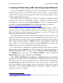
1. Getting Started Using UM: Simulating Hybrid Models
The UM FEM additional module gives the user a possibility to create models of
mechanical systems that include both rigid and elastic bodies, so called hybrid
systems. Elastic displacements assumed to be rather small and describable by finite
element method and linear theory.
This manual helps you to study main features of creating and analyzing hybrid
systems using Universal Mechanism software. Detailed information about
UM FEM you can find in the 11_UM_FEM.pdf of UM user’s manual, which is
available in the {um_root}\manual directory and in the Internet via this link:
http://www.umlab.ru/download/50/eng/11_um_fem.pdf.
It is supposed that you already studied the gs_UM.pdf1 manual, which is
devoted to basics of UM modeling and know how to create new model, add new
bodies and joints, generate and compile equations of motion (UM Input) and
simulate mechanical systems (UM Simulation).
The modal approach is used for simulation of dynamics of elastic bodies. This
approach consists in presentation of elastic deformations with the help of a set of
eigenmodes and static modes2. The approach assumes describing elastic bodies in
terms of finite-element method in ANSYS software with subsequent export that
data to UM. Thus, the necessary condition of using UM FEM is availability the
ANSYS software for some preliminary analysis and calculations.
Every elastic body is considered as a separate subsystem. Data file of the elastic
subsystem is a binary input.fss file. This file may be created with the help of
ANSYS_UM.EXE program or with the help of Wizard of elastic subsystems in
the UMInput.exe. In the latter case ANSYS_UM.EXE creates intermediate
uminput.fum, that contains input data for the Wizard.
After ANSYS_UM.EXE creates input.fss or input.fum files the subsequent
preparing of the model is fulfilled with the help of Universal Mechanism. Since the
data files about elastic body is exported from the ANSYS software and prepared
by ANSYS_UM program ANSYS software is not used any more. Complete data
flow from ANSYS to UM is shown in the eleventh part of UM user’s manual
(part11.pdf). Thus using UM FEM module is possible if ANSYS software is
available on the user’s computer.
1
http://www.umlab.ru/download/50/eng/gs_um.pdf
Please find more detailed information about static modes and eigenmodes in the eleventh part of UM user’s manual
(11_UM_FEM.pdf)
2
Universal Mechanism 5.0
Note.
2
Getting Started: UM FEM
(1) Before coming to the rest part of the manual please check if the
UM FEM module is available on your computer. Run UM
Simulation and from the Help menu select About. The list of
available modules is shown in the Configuration section.
(2) Please also check if the ANSYS software is available on your
computer. If you do not have ANSYS on your computer you will
have to leave some parts of this lesson, where working under ANSYS
environment is considered. But nevertheless you will be able to
complete the lesson using files prepared in advance.
Copyright and trademarks
This manual is prepared for informational use only, may be revised from time to
time. No responsibility or liability for any errors that may appear in this document
is supposed.
Copyright © 2008 Universal Mechanism Software Lab. All rights reserved.
All trademarks are the property of their respective owners.
Universal Mechanism 5.0
3
Getting Started: UM FEM
1.
GETTING STARTED USING UM: SIMULATING HYBRID MODELS ..................... 1
2.
SLIDER-CRANK MECHANISM ............................................................................... 4
2.1.
Preparing ANSYS environment .................................................................................... 6
2.2.
Preparing con-rod as an elastic beam ........................................................................... 7
2.2.1.
Working under ANSYS environment ....................................................................... 7
2.2.2.
Wizard of elastic subsystems ................................................................................. 10
2.3.
Creating the model ...................................................................................................... 17
2.3.1.
Creating graphical objects ...................................................................................... 18
2.3.2.
Creating rigid bodies.............................................................................................. 20
2.3.3.
Creating elastic subsystem ..................................................................................... 21
2.3.4.
Creating joints ....................................................................................................... 22
2.3.5.
Preparing for simulation ........................................................................................ 24
2.4.
3.
Simulation .................................................................................................................... 25
ELECTRIC MOTOR ON ELASTIC PLATFORM.................................................... 31
3.1.
Preparing elastic platform .......................................................................................... 33
3.1.1.
Working under ANSYS environment ..................................................................... 34
3.1.2.
Wizard of elastic subsystems ................................................................................. 35
3.2.
Creating the model and analyzing its dynamics ......................................................... 36
3.2.1.
Introducing elastic platform ................................................................................... 36
3.2.2.
Attaching the elastic platform to a base .................................................................. 36
3.2.3.
Creating graphical elements ................................................................................... 37
3.2.4.
Force elements ....................................................................................................... 40
3.2.5.
Model of electric motor ......................................................................................... 44
3.2.6.
Adding motor to object as a subsystem .................................................................. 44
3.2.6.1. Setting angular velocity of the rotor ................................................................... 46
3.2.7.
Electric motor and platform coupling by force elements......................................... 49
3.2.8.
Preparing for simulation ........................................................................................ 50
3.2.9.
Simulation ............................................................................................................. 51
3.2.9.1. Calculating the equilibrium position and natural frequencies .............................. 52
3.2.9.2. Integration of equations of motion ..................................................................... 55
Universal Mechanism 5.0
4
Getting Started: UM FEM
2. Slider-crank mechanism
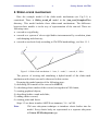
Here the example model of the slider-crank mechanism (see Fig. 2.1) is
considered. There is Slider_crank_all model in the {um_root}\Samples\Flex
directory. This model includes three slider-crank mechanisms. The difference
between these models is in the way of representation of the con-rod. There are
following cases:
· con-rod as a rigid body;
· con-rod as a system of eleven rigid bodies interconnected by revolution joints
with damping and elasticity;
· con-rod as an elastic body according to UM FEM methodology, see Sect. 11.1.
4
1
2
3
Figure 2.1. Slider-crank mechanism: 1 – base, 2 – crank, 3 – con-rod, 4 – slider.
The process of creating and simulating a hybrid model of the slider-crank
mechanism with elastic con-rod is discussed in this section.
Preparing the model consists of the following steps:
1) describing FEA-model of the con-rod in ANSYS;
2) calculating elastic modes of the con-rod, saving data in UM format;
3) creating graphical objects;
4) describing bodies: crank and slider;
5) adding elastic con-rod;
6) creating joints and forces.
Steps 1-2 are done in under ANSYS environment, 3-6 – in UM.
Note.
UM uses subsystem technique to introduce elastic bodies into the
model. Every elastic body are represented as a separate subsystem
of Linear FEM subsystem type.
Universal Mechanism 5.0
5
Getting Started: UM FEM
Create a directory for the future models. Within this section we address this
directory as «.\». This directory will include two subdirectories:
· flexbeam for an elastic beam data;
· slider_crank_fem for the hybrid model.
You can read this manual more or less detailed. Please note the following
remarks.
· If ANSYS software is available on your computer and you want to study all the
data flow in details you should read this manual sequentially.
· If ANSYS software is not available or you want to omit the step of preparing
data in ANSYS you can directly start from the sect. 2.2.2 of this manual. Before
that you should copy the {um_root}\Samples\Flex\flexbeam\input.fum to the
.\flexbeam directory.
· You can omit all the steps of elastic body data preparing. Before that you
should copy {um_root}\Samples\Flex\flexbeam\input.fss to the .\flexbeam
and start reading from the sect. 2.3 of this manual.
Universal Mechanism 5.0
6
Getting Started: UM FEM
2.1. Preparing ANSYS environment
We will use ANSYS software for preparing data for simulation of dynamics of
elastic body. After creating FEA model a calculation of the static and eigen-modes
starts. Macro um.mac is used for such a calculation. Then ANSYS_UM program
starts. This program translates data, that are produced by um.mac into UM format.
Copy the um.mac file from {um_root}\bin to ANSYS default directory for
macros. It is usually the .\docu directory in ANSYS 5.0, .\apdl in ANSYS 7.0-9.0
root directory. Otherwise you need to set search path with the ANSYS command
/PSEARCH,Path_to_macro
After preparing data the um.mac macros runs the external ansys_um.exe program
for subsequent analysis of obtained data. The ansys_um.exe is situated in the
{um_root}\bin directory. You need to open the um.mac in any text editor and edit
the path to the ansys_um.exe program in the last line of the macros. Set full path
to the ansys_um.exe as the parameter of the /sys command. For example,
/sys,c:\um\bin\ansys_um.exe
Note 1.
If the full path to the ansys_um.exe program contains space(s) then
use inverted commas. For example,
/sys,”c:\universal mechanism\bin\ansys_um.exe”
Note 2.
Path to the ansys_um.exe program should contain the Latin letters
only.
Universal Mechanism 5.0
7
Getting Started: UM FEM
2.2. Preparing con-rod as an elastic beam
As it mentioned above, preparing data for introducing elastic bodies into hybrid
models contains the stage of solution of eigen-values problem. There are two
possible mathematical formulations of this problem:
· with diagonal mass matrix;
· with consistent mass matrix.
The {um_root}\Samples\Flex\flexbeam\input directory contains two
subdirectories: lumped and consistent. The first one includes an ANSYS
command file for the case of diagonal mass matrix, the second one – for consistent
mass matrix.
In the manual we will consider the case with diagonal mass matrix.
2.2.1.
Working under ANSYS environment
1. Copy
the
flexbeam&mass21.ans
file
from
the
{um_root}\Samples\Flex\flexbeam\input\lumped directory to the .\flexbeam
directory. This file is the ANSYS command file, uses APDL language and
describes the process of ANSYS model creation. This file also contains
comments that explain every step of the process.
2. Run ANSYS Interactive and select the .\flexbeam directory as working
directory and set Working directory to .\flexbeam, for example
d:\models\flexbeam.
3. Run ANSYS. From the File menu select Read Input from and choose
.\flexbeam&mass21.ans. Steel beam of 2 m length and square cross section
with 2 cm width is created. Finite element model consists of 100 elements of
BEAM4 type and 200 elements of MASS21 type. Two end nodes are
automatically selected as interface nodes1. If you made all setting ANSYS
environment correctly then the um.mac macros is started automatically and
calculates 12 static modes and 10 eigenmodes of the beam.
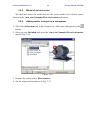
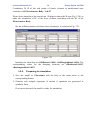
4. If you changed path to the ansys_um.exe program in um.mac properly then
um.mac runs ansys_um.exe automatically. Otherwise run the
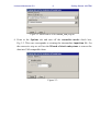
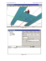
{um_root}\bin\ansys_um.exe manually. The main window of ansys_um
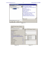
appears, Fig. 2.2.
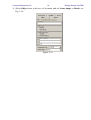
5. Point to the General tab. The ANSYS results file (*.rst) set to
.\flexbeam\flexbeam.rst, Target directory set to .\flexbeam, see Fig. 2.2.
1
More detailed information about interface nodes you can find in the eleventh part of UM User’s Manual
Universal Mechanism 5.0
8
Getting Started: UM FEM
Figure 2.2. Main window of the ANSYS_UM program.
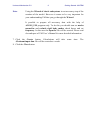
6. Point to the Options tab and turn off the normalize modes check box,
Fig. 2.3. This case corresponds to creating the intermediate input.fum file. On
the successive step we will use the Wizard of elastic subsystems to convert the
data into UM-compatible form.
Figure 2.3.
Universal Mechanism 5.0
Note.
9
Getting Started: UM FEM
Using the Wizard of elastic subsystems is not necessary step of the
creation of the model. However it seems to be very important for
your understanding UM that you go through the Wizard.
It possible to prepare all necessary data with the help of
ANSYS_UM program only. To do this you should turn on modes
normalize and exclude rigid body modes check boxes and set
frequency. In this case the input.fss file will be created. Please read
eleventh part of UM User’s Manual for more detailed information.
7. Click the Create button. Calculations will take
.\flexbeam\input.fum file will be created as a result.
8. Click the Close button.
some
time.
The
Universal Mechanism 5.0
2.2.2.
10
Getting Started: UM FEM
Wizard of elastic subsystems
During the next step we will use the wizard of flexible subsystem data. It is a
tool for animation of elastic modes, and exclusion of some of them.
Note.
Using the wizard of flexible subsystem data is not an obligatory
phase. Preparing the data can be fulfilled with the help of ansys_um
program. To do this point to the Options tab and turn on the
normalize modes and exclude rigid body modes check boxes and
set frequency value, Fig. 2.3. Nevertheless now we will use the
wizard of flexible subsystem data in order to familiarize you with it.
The intermediate input.fum file contains static modes and eigenmodes. To
finish preparing data it is necessary to orthogonalize modes. It may be done
directly in the ansys_um program and if necessary with the help of wizard of
flexible subsystem data.
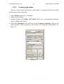
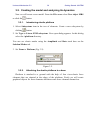
1. Run UM Input program (uminput.exe).
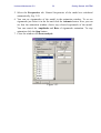
2. Click the Tools/Preparing flexible subsystems menu item. The main window
of the wizard of flexible subsystem data appears.
3. Click the and select a file for the Data file, Fig. 2.4, 2.5.
Figure 2.4
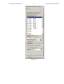
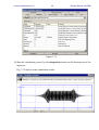
Wizard loads and shows the data, Fig. 2.6. The General tab shows summary
information about elastic subsystem, see Fig. 2.6.
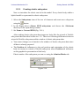
The Position tab (see Fig. 2.7) is used for setting position and orientation of the
elastic body. These transformations influence on the representation of the elastic
body in the animation window of the wizard. Flexible body in the starting position
coincides with X-axis that is not really comfortable to watch. Now we will shift the
beam along Z axis with 0.3 m.
4. Point to the Position tab.
5. Set Shift/z to 0.3, see Fig. 2.7.
Universal Mechanism 5.0
11
Getting Started: UM FEM
Figure 2.5
Figure 2.6
Figure 2.7
Universal Mechanism 5.0
12
Getting Started: UM FEM
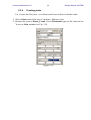
Using the Image tab we can change graphical representation of the FE-model.
There are two modes of such a representation: simplified and full. During the full
model status line shows the information about nodes and finite elements when
mouse cursor is on it. However the full mode takes more CPU time to animate.
6. Set Image to full.
7. Turn off the Image parameters/draw nodes check box.
8. Set the rest parameters according to the Fig. 2.8.
Figure 2.8
Note.
Single node finite elements of the MASS21 type are used for
setting moment of inertia of the body relative to the longitudinal
axis. Set Sizes/Single node FE to 0 in order to hide such elements
and make the image clearer.
Universal Mechanism 5.0
13
Getting Started: UM FEM
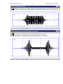
The Solution tab gives you a possibility to animate modes of elastic subsystem.
To start animation you should click the Animate button, see Fig. 2.9. You can
control this animation with the help of Amplitude and Rate track bars.
You can include/exclude any form from the final set of modes turning on/off
the corresponding check boxes in the Modes tab. The more modes you include in
the final solution and the more frequency these modes have the more accurate and
time-consuming subsequent numerical integration you have. Generally it is
recommended to turn on/off modes to keep a balance between solution accuracy
and time efforts for it.
Thus, you can fulfill the only calculation in the ANSYS software with the
maximum modes you will ever use (10 in this example) and then form various sets
of modes with the help of the Wizard of flexible subsystems data.
Leave the initial set of modes without any changes.
Universal Mechanism 5.0
14
Figure 2.9
Getting Started: UM FEM
Universal Mechanism 5.0
15
Getting Started: UM FEM
9. Turn on the Transformations / exclude rigid body modes (Fig. 2.9).
10. Set Transformations / Frequency to 0.3 (Fig. 2.9).
11. Click the Transform button and confirm this action in the subsequent dialog.
As a result the transformed set of modes of elastic body is created. In the case
of successful execution of the transformation the following message appears, see
Fig. 2.10.
Figure 2.10
Note.
The initial set of modes includes rigid body modes, which should
be excluded according to the used approach for simulation. Rigid
body modes theoretically correspond to zero frequencies, but in fact
because of using numerical methods and round-off errors these
frequencies are small and close to zero but not exact zero.
In fact the Transformations / Frequency field indicates the
threshold value and all frequencies that are less than this value are
supposed to correspond to rigid body modes.
Now we need to save the transformed data set.
12. Point to Transformed in the Data set group, Fig. 2.11.
Figure 2.11
13. Click the Save as button. In the dialog set Path to subsystem data and click
the Save button, see Fig. 2.12. Please, note, that the latter directory will further
serve as a subsystem name.
Universal Mechanism 5.0
16
Figure 2.12
Preparing the data for flexible subsystem is done.
Getting Started: UM FEM
Universal Mechanism 5.0
17
Getting Started: UM FEM
2.3. Creating the model
The hybrid model of the slider-crank mechanism includes two rigid bodies, one
elastic body and four joints.
Bodies:
· crank, 1 m length;
· con-rod, 2 m length;
· slider.
The crank and the slider are rigid bodies, con-rod is elastic subsystem (in terms
of UM).
Joints:
· revolution joint between Base0 and the crank, crank and the con-rod, and the
con-rod and the slider;
· translational joint between slider and Base0.
1. Create a new model. Point the File/New object MBS menu command or click
the
button. New constructor window appears.
Universal Mechanism 5.0
2.3.1.
18
Getting Started: UM FEM
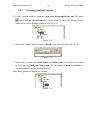
Creating graphical objects
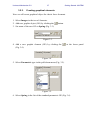
1. Load a graphical object from the {um_root}\bin\graph\Base1.umi file using
button or Edit | Read from file… menu item. Element «NoName» will be
added to the list of graphic elements, see Fig. 2.13.
Figure 2.13
2. Select this element and set name to Base0 in the data inspector (Fig. 2.14).
Figure 2.14.
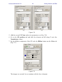
3. Repeat these actions for Crank1.umi and Slider1.umi files, which are located
in the directory {um_root}\bin\graph. Set the names Crank and Slider to
created graphical objects correspondently.
Thus, three graphical objects are created.
Figure 2.15
Universal Mechanism 5.0
19
Getting Started: UM FEM
4. Select Object item in the tree of elements and set Scene image to Base0, see
Fig. 2.16.
Figure 2.16
Universal Mechanism 5.0
2.3.2.
20
Getting Started: UM FEM
Creating rigid bodies
Here we create slider and crack as rigid bodies, set graphical objects for them
and set their inertia parameters.
1. Select Bodies in the tree of elements.
2. Add two new bodies.
3. Rename bodies with Slider and Crank and set the correspondent graphical
objects (Slider and Crank).
4. Select the Parameters tab and turn on the Compute automatic flag for the
both of bodies. Inertia property of the bodies are computed automatically, see
Fig. 2.17.
Figure 2.17.
Universal Mechanism 5.0
2.3.3.
21
Getting Started: UM FEM
Creating elastic subsystem
Now we introduce the elastic con-rid in the model. Every elastic body within a
hybrid model is represented as elastic subsystem.
1. Select the Subsystems item of the tree of elements and create new subsystem
using the
button.
2. In the Type select «Linear FEM subsystem» and choose the .\flexbeam
directory in the open dialog window.
3. Set Name to Con-rod FEM (Fig. 2.18.).
After reading elastic subsystem data inspector looks like the wizard of flexible
subsystem data described in the sect. 2.2. There are following differences between
wizard of flexible subsystem and the window of elastic subsystem data.
· You cannot changes set of modes in the window of elastic subsystem data since
all data is already prepared.
· The Position tab influences to the real position and orientation of the elastic
body in contrast to wizard of flexible subsystem where Position tab influences
on the graphical representation of the body.
Elastic modes of the subsystem you can see using the Solution/Modes tab.
Figure 2.18.
Universal Mechanism 5.0
2.3.4.
22
Getting Started: UM FEM
Creating joints
Let’s create the first joint – revolution joint between Base0 and the crank.
1. Select Joints item of the tree of elements. Add new joint.
2. Rename the joint to Base0_Crank. Select Rotational type for the joint and set
Y axis as Joint vectors, see Fig. 2.19.
Figure 2.19.
Universal Mechanism 5.0
23
Getting Started: UM FEM
3. Select the Joint force tab, set Joint torque to Expression and in the field
Description of force set F = torque - cdiss_crank * v, see Fig. 2.20. Press Enter.
The window Initialization of values for new identifiers appears. Set identifiers
value as follows: torque = 100, cdiss_crank = 10.
Figure 2.20.
4. Add the rest three joints as it is shown in the Fig. 2.21.
Figure 2.21.
Universal Mechanism 5.0
2.3.5.
24
Getting Started: UM FEM
Preparing for simulation
1. Save the model as Slider_crank_fem (File/Save as menu command), see
Fig. 2.22.
Figure 2.22.
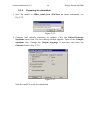
2. Generate and compile equations of motion. Click the Object/Generate
equations menu item. The new dialog window appears. Turn on the Compile
equations flag. Change the Output language if necessary and click the
Generate button (Fig. 2.23.).
Figure 2.23.
Now the model is ready for simulation.
Universal Mechanism 5.0
25
Getting Started: UM FEM
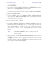
2.4. Simulation
1. Use the menu command Object/Simulation to run UM Simulation program.
Main window of the UM Simulation program appears.
Let’s obtain reaction forces in the joints Crank_Con-rod and Con-rod_Slider.
2. Open new animation window.
3. From the Analysis menu select Simulation. Object simulation inspector
appears. Select the FEM subsystems/Image tab to set up animation parameters
of the elastic con-rod as you want.
Now we will calculate initial conditions.
4. In the Object simulation inspector select the Initial conditions tab. Select the
Con-rod subsystem in the drop down list, Fig. 2.24. An anchor sign means that
the correspondent degree of freedom is frozen. In this example it means that the
elastic degrees of freedom will not be changed during calculation of initial
position.
Note.
If the Initial condition tab differs to the Fig. 2.24 set the
anchors manually.
5. Make sure that the Autocalculation of constraint equations mode is turned on
(the
button should be pressed), otherwise press this button. Then calculate
the initial conditions by clicking the
button. Animation window shows the
current position of the mechanism, Fig. 2.25.
Universal Mechanism 5.0
26
Getting Started: UM FEM
Figure 2.24.
Figure 2.25.
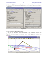
6. Open new graphical window (Tools/Graphical window menu command).
7. Run Wizard of variables and create variables for reaction forces according to
Fig. 2.26 and drag them to the graphical window.
Universal Mechanism 5.0
27
Getting Started: UM FEM
Figure 2.26.
8. Select the Object simulation inspector and point to the Solver tab. Set the
following parameters:
· Solver = Park,
· Type of solving = Range Space Method,
· Simulation time = 2.0.
· Step size for animation = 0.001.
· Error tolerance = 1E-7.
· Computing Jacobian matrices = on (always default).
· Block-diagonal matrices = off.
Figure 2.27.
Universal Mechanism 5.0
28
Getting Started: UM FEM
9. Select the FEM Subsystems/Simulation tab and set up all options according to
Fig. 2.28.
Figure 2.28.
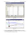
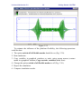
10. Start simulation (Integration button).
You can see movement of the mechanism in the animation window (see
Fig. 2.29) and oscillograms of reaction forces in the graphical window (see
Fig. 2.30).
Figure 2.29. Animation window
Universal Mechanism 5.0
29
Getting Started: UM FEM
Figure 2.30. Graphical window
In order to estimate the influence of the elastic con-rod instead rigid one, open
the {um_root}\Samples\Flex\Slider_crank_all model. Graphs of the reaction
force are shown in the Fig. 2.31.
1
2
Figure 2.31. Reaction force in the Con-rod _Slider joint
1 – con-rod is a rigid body, 2 – con-rod is an elastic body.
Universal Mechanism 5.0
30
Getting Started: UM FEM
Configuration file example.icf, which is situated in the Slider_crank_all
directory, contains graphical windows with reaction forces in the rest joints of the
model, as well as angular velocities of all cranks.
Universal Mechanism 5.0
31
Getting Started: UM FEM
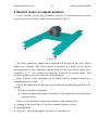
3. Electric motor on elastic platform
Let us consider step by step dynamical analysis of a mechanical system that
consists of an electric motor and an elastic platform, Fig. 3.1.
Figure 3.1.
The elastic platform is connected to a ground with the help of four visco-elastic
linear force elements. The electric motor is included to a model as an external
subsystem and is also connected with the help of four visco-elastic linear force
elements, Fig. 3.1. An eccentric is attached to a rotor of the electric motor. This
eccentric produces forced oscillations of the platform.
Basic features of the description of the model and its dynamical analysis is
considered in this section.
During the simulation we will analyze the following dynamical properties of the
system:
· forces in the force elements;
· vertical displacements and accelerations of the platform in the center part
under the motor.
Here we will simulate the following sequence of operation modes:
· running of the rotor from ω=0 up to its nominal angular velocity.
· operating duty;
· stop way – decreasing angular velocity of a rotor till ω=0.
Universal Mechanism 5.0
32
Getting Started: UM FEM
Preparing the model includes the following steps:
· preparing data of the elastic platform;
· introducing FEA-model of the platform into the final UM-model;
· attaching the elastic platform to a ground;
· creating the model of the electric motor;
· introducing the electric motor into the final model as an external
subsystem;
· attaching the electric motor to the platform with the help of visco-elastic
elements.
Let us consider all of the described above steps in details. At that main attention
will be put to the features that were not considered in the previous section.
It supposes that you already finished the previous section that is why some
comments here are given shortly.
Please choose an existing or create a new directory for the future model. Within
this section we will address this directory as «.\». Create two subdirectories:
· .\Vibrostand for the final composite model;
· .\Vibrostand\Platform for elastic platform.
Universal Mechanism 5.0
33
Getting Started: UM FEM
3.1. Preparing elastic platform
In terms of Universal Mechanism software every elastic body is considered as a
separate subsystem of Linear FEM subsystem type. Standard save file for such a
subsystem is input.fss file. Preparing the elastic platform includes the following
steps:
1) description the FEA model of the platform in ANSYS software;
2) calculation of the elastic modes and export result from ANSYS in UM format.
There are two possible ways to fulfill the second step:
1) generate the input.fss file directly by ANSYS_UM.EXE program;
2) firstly generate the intermediate input.fum file by the ANSYS_UM.EXE and
then complete data transformations with the help of Wizard of elastic
subsystems that is a tool within the UM Input program. This wizard gives the
user a possibility to visualize calculated elastic forms and exclude some modes
from the final set of elastic modes (input.fss).
There are three files in the {um_root}\Samples\Flex\platform: input.fss,
input.fum and platformshell63.ans.
· If you want to omit the step of preparing the data in ANSYS but familiarize
yourself with Wizard of elastic subsystems you should copy the {um_root}\
Samples\Flex\input.fum file to the .\platform directory and go to the
sect. 3.1.2 of this manual.
· You may omit all the steps of creating the data of elastic platform, in this case
you should copy the {um_root}\Samples\Flex\platform\input.fss file to the
.\platform directory and go to the sect. 3.2 of this manual.
Universal Mechanism 5.0
3.1.1.
34
Getting Started: UM FEM
Working under ANSYS environment
Before you come to the next step please repeat all the steps from the sect. 2.1.
Now we will create the FEA model of the platform and export the data for the
subsequent using them under UM environment.
1. Copy
the
platformshell63.ans
file
from
the
{um_root}\Samples\Flex\platform directory to the .\platform directory. This
file contains APDL commands that automatize creating the FEA model of the
platform.
2. Run ANSYS Interactive and select the .\platform directory as a working
directory.
3. Run ANSYS.
4. From the File menu select the Read Input from and open the
platformshell63.ans file. As a result a steel platform that is consists of two
beams of 1m length and a shelf between them.
This finite-element model includes 886 elements of SHELL63 type. Width of all
elements is 5 cm. You can open platformshell63.ans in any text editor and change
some of parameters of the FEA model, see comments in the body of this file. Four
nodes, where the platform is connected with the ground, are selected as interfaced
nodes. In the end the um.mac is run. If the um.mac is not run automatically you
should run it manually, see Sect. 2.1. As a result of the um.mac execution 24 static
modes and 10 eigenmodes are calculated.
5. If the path to the ANSYS_UM.EXE in the um.mac is set correctly (see
Sect. 2.1), ANSYS_UM.EXE starts automatically. Otherwise run
ANSYS_UM.EXE manually from the {um_root}\bin directory.
6. Transform data according the 5-8 items of the Sect. 2.2.1.
Universal Mechanism 5.0
3.1.2.
35
Getting Started: UM FEM
Wizard of elastic subsystems
Working with the Wizard of elastic subsystems is described in the Sect. 2.2.2.
Now you should repeat all the instructions from the Sect. 2.2.2. Use the
.\platform\input.fum as an input file for the Wizard. Please, note, that the
.\platform\input.fss file should be created after all.
Universal Mechanism 5.0
36
Getting Started: UM FEM
3.2. Creating the model and analyzing its dynamics
Now we will create a new model. From the File menu select New object MBS
or click the
3.2.1.
button.
Introducing elastic platform
1. Select Subsystems item in the tree of elements. Create a new subsystem by
clicking
button.
2. Set Type to Linear FEM subsystem. New open dialog appears. In this dialog
select the .\platform directory.
You can see elastic modes using the Amplitude and Rate track bars on the
Solution/Modes tab.
3. Set Name to Platform (Fig. 3.2).
Figure 3.2.
3.2.2.
Attaching the elastic platform to a base
Platform is attached to a ground with the help of four visco-elastic force
elements that are situated at the edges of the platform. Firstly we will create
graphical objects for force elements and then create force elements themselves.
Universal Mechanism 5.0
3.2.3.
37
Getting Started: UM FEM
Creating graphical elements
Now we will create graphical object for elastic force elements.
1. Select Images in the tree of elements.
2. Add new graphic object (GO) by clicking the
3. Set name of the new GO to Spring (Fig. 3.3).
button.
Figure 3.3.
4. Add a new graphic element (GE) by clicking the
(Fig. 3.4).
at the lower panel
Figure 3.4.
5. Select Parametric type in the pull-down menu (Fig. 3.5).
Figure 3.5.
6. Select Spring in the list of the standard parametric GE (Fig. 3.6)
Universal Mechanism 5.0
38
Figure 3.6.
7. Set parameter values as in Fig. 3.7
Fugure 3.7.
Let us add now a GE for the damping force element.
1.
2.
3.
4.
Add a new GO
Rename it as Damper.
Add a new GE to the GO.
Set its type as Cone and parameters as in Fig. 3.8a.
Getting Started: UM FEM
Universal Mechanism 5.0
39
a)
Getting Started: UM FEM
b)
Figure 3.8.
5. Add the second GE Cone and set its parameters as in Fig. 3.8b
6. Go to the GE position tab and shift the element on 0.3 along Z axis (the
Translation | z box).
7. Set the diffuse component of the GE color by Diffuse button on the Color tab
(Fig. 3.9)
Figure 3.9
The images are created. Let us continue with the force elements.
Universal Mechanism 5.0
3.2.4.
40
Getting Started: UM FEM
Force elements
Let us introduce several identifiers to set the attachment points:
· BeamLength – the length of platform beams;
· WidthShelf – the width of connecting shelf;
· WidthBeamShelfLow – the width of lower shelf of beam section.
Let us start with the elastic element on the front left end of the platform beam.
1. Select Linear forces in the object element list.
2. Add a new force element by clicking the
button.
3. Rename it as SpringFL (forward, left), set element type Elastic, interacting
bodies Base0-Platform.Platform as well as the Spring GO (Fig. 3.10).
4. Set coordinates of element attachment points to the first body Base0:
BeamLength/2, -WidthShelf/2-WidthBeamShelfLow/2, – 0.05;
Initialize values of identifiers as (Fig. 3.12)
BeamLength=1.0, WidthShelf=0.4, WidthBeamShelfLow=0.1
5. Coordinates of the element end point in undeformed state in system of
coordinates of the first body, Fig. 3.10:
BeamLength/2, -WidthShelf/2-WidthBeamShelfLow/2, 0.
6. Select Body2 tab. Set coordinates of element attachment points to the second
body Platform.Platform (Fig. 3.11):
BeamLength/2, -WidthShelf/2-WidthBeamShelfLow/2, 0;
Universal Mechanism 5.0
41
Getting Started: UM FEM
Figure 3.10
Figure 3.11
Figure 3.12
5. Let us introduce a stiffness matrix of the element. Select Parameters tab. Click
the button in the Stiffness matrix box (Fig. 3.13), set diagonal elements of
the matrix corresponding to the translational degrees of freedom (Fig. 3.14),
and click OK. Set the following identifier values: cxx=1e+6, cyy=1e+6,
czz=1e+6 (N/m).
Figure 3.13
Universal Mechanism 5.0
42
Getting Started: UM FEM
Figure 3.14
The elastic force element is described.
Now let us describe the front left damping element.
1. Copy the linear force element by the
button.
2. Rename the new element as DamperFL (forward, left), set the element type
Dissipative and set GO to Damper (Fig. 3.15).
Figure 3.15
4. Let us set dissipative matrix of the element. Select Parameters tab. Click the
button in the Dissipative matrix box, set the diagonal elements of the matrix
corresponding to the translational degrees of freedom dxx, dyy, dzz, and click
OK. Set the following identifier values dxx=1E3, dyy=1E3, dzz=1E3 (Ns/m).
Damping element is described.
Universal Mechanism 5.0
43
Getting Started: UM FEM
Create the rest three pairs of force element quite similar to the previous ones.
Use the
button to copy the description. Do it in the following manner.
1. Select previously described element of the necessary type, e.g. SpringFL in the
case of a new elastic element.
2. Click the
button to create a copy.
3. Rename the copy, e.g. SpringFR (forward, right).
4. Correct coordinates of attachment points. For the SpringFR element we have
Base0:
BeamLength/2, WidthShelf/2 + WidthBeamShelfLow/2, –0.05;
Platform.Platform:
BeamLength/2, WidthShelf/2 + WidthBeamShelfLow/2, 0.0;
coordinates of the element end point in undeformed state in system of
coordinates of the first body:
BeamLength/2, WidthShelf/2 + WidthBeamShelfLow/2, 0.0 (Fig. 3.10)
Thus, the full list of force elements connecting the platform with the base must
include the following elements: SpringFL, DamperFL, SpringFR, DamperFR,
SpringBL, DamperBL, SpringBR, DamperBR.
Universal Mechanism 5.0
3.2.5.
44
Getting Started: UM FEM
Model of electric motor
We shall not create the model but use the ready model of an electric motor
located in the {um_root}\Samples\Flex\electricmotor directory.
3.2.6.
Adding motor to object as a subsystem
1. Select the Subsystems tab in the element list. Add a new subsystem by the
button.
2. Select its type Included and open the {um_root}\Samples\Flex\electricmotor
model (Fig. 3.16).
Figure 3.16
3. Rename the subsystem as Electricmotor.
4. Set the subsystem location as in Fig. 3.17.
Universal Mechanism 5.0
45
Figure 3.17
Getting Started: UM FEM
Universal Mechanism 5.0
46
Getting Started: UM FEM
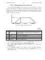
3.2.6.1. Setting angular velocity of the rotor
Let us set the law for angular velocity of the rotor as it shown in Fig. 3.18. Here
we can see three modes: speeding up, a working mode and a braking mode. During
speeding up and braking angular acceleration is constant and angular velocity
changes linearly, see Fig. 3.18. The law from Fig. 3.18 is parameterized with the
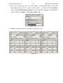
help of six identifiers, see table 1.
w
omega
t
tstart
tspeeding_up
tworking
tbraking
Fig. 3.18. Angular velocity of the rotor
Table 1.
Identifiers
1
Identifier
Nu
2
3
4
5
6
omega
tstart
tspeeding_up
tworking
tbraking
Meaning
Nominal angular velocity of the rotor, revolutions per
minute (r.p.m.)
Nominal angular velocity of the rotor, rad/s
Time before speeding up, s
Time of speeding up mode, s
Time of working mode, s
Time of braking mode, s
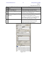
1. Click the Edit subsystem button to edit the Electricmotor subsystem, see
Fig. 3.17. New object constructor for the Electricmotor appears.
2. Select Joints | jRotor->Body in the tree of elements. It is a joint of the
Generalized type.
3. In the Inspector window in the right part select the RTx elementary
transformation (Fig. 3.19). This time function is set as time-table of 5 rows, see
table 2 and Fig. 3.19.
Universal Mechanism 5.0
47
Table 2.
Time-table for the rotor.
Expression
Time interval
№
1 Tstart
2 tstart+tspeeding_up
3 tstart+tspeeding_up+tworking
4
5
Getting Started: UM FEM
0
(omega/tspeeding_up)*sqr(t-tstart)/2
(omega/tspeeding_up)*sqr(tspeeding_up)/2+
omega*(t-tstart-tspeeding_up)
tstart+tspeeding_up+tworking+ (omega/tspeeding_up)*sqr(tspeeding_up)/2+
tbraking
omega*tworking+omega*(t-tstarttspeeding_up-tworking)-(omega/tbraking)*
sqr(t-tstart-tspeeding_up-tworking)/2
100
(omega/tspeeding_up)*sqr(tspeeding_up)/2+
omega*tworking+omega*(tworking)(omega/tbraking)*sqr(tbraking)/2
Figure 3.19
Universal Mechanism 5.0
48
Getting Started: UM FEM
4. Close the constructor window of the Electricmotor and come back to the
composite model.
Universal Mechanism 5.0
3.2.7.
49
Getting Started: UM FEM
Electric motor and platform coupling by force elements
Coupling the electric motor and the platform can be set quite similar to
attaching the platform to the base. Electricmotor.Body and Platform.Platform
are interacting bodies. An example of description of an elastic force element is
shown in Fig. 3.20.
Figure 3.20
Table l contains coordinates of attachment points of elastic and damping force
elements realizing the coupling.
Force element
SpringMotorFL,
DamperMotorFL
SpringMotorFR,
DamperMotorFR
SpringMotorBL,
DamperMotorBL
SpringMotorBR,
DamperMotorBR
Electricmotor.Body
X
Y
Z
Table 1
Platform.Platform
X
Y
Z
0.01560.015
0.053
-0.069+
0.015
0.01560.015
-0.069+
0.015
0.06
0.01560.015
0.053
0.1-0.015
0.01560.015
0.1-0.015
0.06
-0.1+
0.015
0.053
-0.069+
0.015
-0.1+
0.015
-0.069+
0.015
0.06
-0.1+
0.015
0.053
0.1-0.015
-0.1+
0.015
0.1-0.015
0.06
Universal Mechanism 5.0
50
Getting Started: UM FEM
Coordinates X, Z of the end points of elastic element in undeformed state
coincides with Electricmotor.Body, Y=0.07.
Please draw attention to the rotation on -90 degrees about the X axis (Fig. 3.20), to
make the orientation of SC of the force element coinciding with the SC of the
Electricmotor.Body.
Set the stiffness matrices of elastic force element as it is shown in Fig. 3.21.
Figure 3.21
Initialize the identifiers as cStifflateral=1.0E6, cStifflongitudinal=1.0E6. The
corresponding values for the damping elements are cDisslateral=1.0E3,
cDisslongitudinal=1.0E3.
3.2.8.
Preparing for simulation
1. Save the model as Vibrostand with the help of the main menu or the
corresponding button.
2. Generate and compile equations of motion if equations are generated in
symbolic form.
If no errors detected, the model is ready for simulation.
Universal Mechanism 5.0
3.2.9.
51
Getting Started: UM FEM
Simulation
Let us compute the vertical components of forces in force elements coupling the
electric motor and the platform, when the rotor of the motor rotates with the
constant angular velocity nu = 1620 r.p.m. As an example consider the rear right
pair of elements. Let us compute displacements and accelerations of a center of
plate under the electric motor as well.
1. Run the UM Simulation with the F9 key or by clicking the
button on the
tool panel.
2. Open a new animation window to visualize the simulation process,
Tools/Animation window.
3. Use the Analysis | Simulation menu command to open the Object simulation
inspector.
4. Use the FEM Subsystems | Image tab of the Object simulation inspector to
change the flexible platform image if necessary.
Universal Mechanism 5.0
52
Getting Started: UM FEM
3.2.9.1. Calculating the equilibrium position and natural
frequencies
Let us calculate the equilibrium position of the stand.
1. If the Objection simulation inspector is active close it by the Close button.
2. From the Analysis menu select Linear analysis or press the F8 key. Window
of linear analysis appears.
3. Select the Equilibrium tab. Turn on the Keep coordinates and identifiers
check box. Start the calculation by the Compute button, Fig. 3.22.
Calculation process might take some time.
Figure 3.22
Now we need to save current coordinates, which correspond to the found
equilibrium position, to a file of initial conditions.
4. Select the Initial conditions tab. Click the
conditions to the equilibrium.xv file.
Note.
button and save current initial
Just found values of coordinates correspond to equilibrium position
are correct for the current values of identifiers of the model only.
Any changes of identifiers will lead that found above set of
coordinates will not correspond to equilibrium position any more. In
such a case you need to repeat the calculation of equilibrium position.
Universal Mechanism 5.0
53
Getting Started: UM FEM
5. Select the Frequencies tab. Natural frequencies of the model are calculated
automatically, Fig. 3.23.
6. You can see eigenmodes of the model in the animation window. To see an
eigenmode just select it in the list and click the Animate button. Now you can
see that the animation window shows any selected eigenmode of the model.
You can control the Amplitude and Rate of eigenmode animation. To stop
animation click the Stop button.
7. Close the window of Linear analysis.
Figure 3.23
Universal Mechanism 5.0
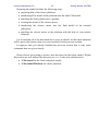
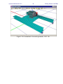
54
Getting Started: UM FEM
Figure 3.24. Animation of second eigenmode, 24.11 Hz
Universal Mechanism 5.0
55
Getting Started: UM FEM
3.2.9.2. Integration of equations of motion
1. Open the Wizard of variables (the Tools | Wizard of variables menu
command) and create variables for Z components of linear force elements
SpringMotorBR, DamperMotorBR, Fig. 3.25.
Figure 3.25
2. Open a new graphical window (the Tools | Graphical window menu
command).
3. Drag the created variables into the graphical window by the mouse.
4. Let us select some node of the FEM-model where we will calculate Z
components of position and acceleration. If the animation window does not
show nodes of FE mesh, select the FEM subsystems / Image. Set Image to
full. Turn on the Image | Draw nodes check box. Set non-zero value in Node
image, for example 3, see Fig. 3.26.
Universal Mechanism 5.0
56
Getting Started: UM FEM
Figure 3.26.
Now we will plot oscillograms of a position and acceleration of some arbitrary
node of the platform.
5. Select Wizard of variables and create two variables for calculation Z projections
of position and acceleration of the node 956 with approximate coordinates
(-0.048; 0.007; 0.06), see Fig. 3.27, 3.28.
Note.
You can plot position and acceleration of any node you want. The only
information you need is coordinates of the node. To get them point the
mouse to the node in an animation window and you can see its
coordinates in the status bar of the window, see Fig. 3.27.
6. Create two new graphical windows (Tools/Graphical window) and drag and
drop just created variables to these windows separately.
Universal Mechanism 5.0
57
Figure 3.27.
Figure 3.28.
Getting Started: UM FEM
Universal Mechanism 5.0
58
Getting Started: UM FEM
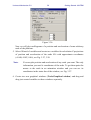
7. Set the solver parameter on the Solver tab of the inspector as in Fig. 3.29:
· Solver = Park;
· Type of solving = Range Space Method (RSM);
· Simulation time = 10.0;
· Step size = 0.002;
· Error tolerance = 1E-8;
· Computing Jacobian Matrices = ON (always for flexible subsystems);
· Block-diagonal matrices = OFF.
Figure 3.29
8. On the FEM subsystems | Simulation tab switches gravity, internal
dissipation as well as linear model should be ON. Set a=0.001, b=0
(Fig. 3.30).
Universal Mechanism 5.0
59
Getting Started: UM FEM
Figure 3.30.
9. Select the Identifiers tab in the Object simulation inspector. Select the
Vibrostand.Electricmotor from the pull-down list of subsystems. Set the
following values (Fig. 3.31):
· nu=1620 (27 revolutions per second);
· tstart=0.5;
· tspeeding_up=2;
· tworking=3;
· tbraking=4.
Note. Rotational speed of the rotor exceeds two first natural frequencies of
the vibrostand that is why there will be resonance conditions during
speeding-up the rotor.
Universal Mechanism 5.0
60
Getting Started: UM FEM
Figure 3.31.
10.Start the simulation process by the Integration button on the bottom part of the
inspector.
Fig. 3.32 depicts some simulation results.
Universal Mechanism 5.0
61
Getting Started: UM FEM
Universal Mechanism 5.0
62
Getting Started: UM FEM
Figure 3.32
To estimate the influence of the platform flexibility, the following operations
could be done.
1. The option switch off all flexible modes should be on (Fig. 3.30).
2. Run simulation.
3. Copy variables in graphical windows as static using popup menus (contact
menu in a graphical window, Copy as static variables menu item).
4. Change the option switch of all flexible modes to off (Fig. 3.30).
5. Repeat the simulation.
6. Compare simulation results.