Download The Art of R Programming

The Art of R Programming
Norman Matloff
September 1, 2009
ii
Contents
1
2
3
Why R?
1
1.1
What Is R? . . . . . . . . . . . . . . . . . . . . . . . . . . . . . . . . . . . . . . . . . . .
1
1.2
Why Use R for Your Statistical Work? . . . . . . . . . . . . . . . . . . . . . . . . . . . . .
1
Getting Started
5
2.1
How to Run R . . . . . . . . . . . . . . . . . . . . . . . . . . . . . . . . . . . . . . . . . .
5
2.1.1
Interactive Mode . . . . . . . . . . . . . . . . . . . . . . . . . . . . . . . . . . . .
5
2.1.2
Running R in Batch Mode . . . . . . . . . . . . . . . . . . . . . . . . . . . . . . .
6
2.2
A First R Example Session (5 Minutes) . . . . . . . . . . . . . . . . . . . . . . . . . . . .
6
2.3
Functions: a Short Programming Example . . . . . . . . . . . . . . . . . . . . . . . . . . .
9
2.4
Preview of Some Important R Data Structures . . . . . . . . . . . . . . . . . . . . . . . . . 10
2.4.1
Vectors . . . . . . . . . . . . . . . . . . . . . . . . . . . . . . . . . . . . . . . . . 11
2.4.2
Matrices . . . . . . . . . . . . . . . . . . . . . . . . . . . . . . . . . . . . . . . . . 11
2.4.3
Lists . . . . . . . . . . . . . . . . . . . . . . . . . . . . . . . . . . . . . . . . . . . 11
2.4.4
Data Frames . . . . . . . . . . . . . . . . . . . . . . . . . . . . . . . . . . . . . . 11
2.5
Startup Files . . . . . . . . . . . . . . . . . . . . . . . . . . . . . . . . . . . . . . . . . . . 12
2.6
Extended Example: Regression Analysis of Exam Grades . . . . . . . . . . . . . . . . . . . 12
2.7
Session Data . . . . . . . . . . . . . . . . . . . . . . . . . . . . . . . . . . . . . . . . . . . 15
Vectors
3.1
17
Scalars, Vectors, Arrays and Matrices . . . . . . . . . . . . . . . . . . . . . . . . . . . . . 17
iii
iv
CONTENTS
3.2
“Declarations” . . . . . . . . . . . . . . . . . . . . . . . . . . . . . . . . . . . . . . . . . . 18
3.3
Generating Useful Vectors with “:”, seq() and rep() . . . . . . . . . . . . . . . . . . . . . . 18
3.4
Vector Arithmetic and Logical Operations . . . . . . . . . . . . . . . . . . . . . . . . . . . 19
3.5
Recycling . . . . . . . . . . . . . . . . . . . . . . . . . . . . . . . . . . . . . . . . . . . . 20
3.6
Vector Indexing . . . . . . . . . . . . . . . . . . . . . . . . . . . . . . . . . . . . . . . . . 20
3.7
Vector Element Names . . . . . . . . . . . . . . . . . . . . . . . . . . . . . . . . . . . . . 21
3.8
Elementwise Operations on Vectors . . . . . . . . . . . . . . . . . . . . . . . . . . . . . . 22
3.9
3.8.1
Vectorized Functions . . . . . . . . . . . . . . . . . . . . . . . . . . . . . . . . . . 22
3.8.2
The Case of Vector-Valued Functions . . . . . . . . . . . . . . . . . . . . . . . . . 24
3.8.3
Elementwise Operations in Nonvectorizable Settings . . . . . . . . . . . . . . . . . 24
Filtering . . . . . . . . . . . . . . . . . . . . . . . . . . . . . . . . . . . . . . . . . . . . . 24
3.10 Combining Elementwise Operations and Filtering, with the ifelse() Function . . . . . . . . . 26
3.11 Extended Example: Recoding an Abalone Data Set . . . . . . . . . . . . . . . . . . . . . . 26
4
Matrices
29
4.1
General Operations . . . . . . . . . . . . . . . . . . . . . . . . . . . . . . . . . . . . . . . 29
4.2
Matrix Indexing . . . . . . . . . . . . . . . . . . . . . . . . . . . . . . . . . . . . . . . . . 31
4.3
Matrix Row and Column Mean Functions . . . . . . . . . . . . . . . . . . . . . . . . . . . 32
4.4
Matrix Row and Column Names . . . . . . . . . . . . . . . . . . . . . . . . . . . . . . . . 32
4.5
Extended Example: Preliminary Analysis of Automobile Data . . . . . . . . . . . . . . . . 33
4.6
Dimension Reduction: a Bug or a Feature? . . . . . . . . . . . . . . . . . . . . . . . . . . . 35
4.7
Adding/Deleting Elements of Vectors and Matrices . . . . . . . . . . . . . . . . . . . . . . 36
4.8
Extended Example: Discrete-Event Simulation in R . . . . . . . . . . . . . . . . . . . . . . 37
4.9
Filtering on Matrices . . . . . . . . . . . . . . . . . . . . . . . . . . . . . . . . . . . . . . 42
4.10 Applying the Same Function to All Rows or Columns of a Matrix . . . . . . . . . . . . . . 43
4.10.1 The apply() Function . . . . . . . . . . . . . . . . . . . . . . . . . . . . . . . . . . 43
4.10.2 The sapply() Function . . . . . . . . . . . . . . . . . . . . . . . . . . . . . . . . . 44
4.11 Digging a Little Deeper on the Vector/Matrix Distinction . . . . . . . . . . . . . . . . . . . 45
CONTENTS
5
v
Lists
47
5.1
Creation . . . . . . . . . . . . . . . . . . . . . . . . . . . . . . . . . . . . . . . . . . . . . 47
5.2
List Tags and Values, and the unlist() Function . . . . . . . . . . . . . . . . . . . . . . . . . 48
5.3
Issues of Mode Precedence . . . . . . . . . . . . . . . . . . . . . . . . . . . . . . . . . . . 48
5.4
Accessing List Elements . . . . . . . . . . . . . . . . . . . . . . . . . . . . . . . . . . . . 49
5.5
Adding/Deleting List Elements . . . . . . . . . . . . . . . . . . . . . . . . . . . . . . . . . 50
5.6
Indexing of Lists . . . . . . . . . . . . . . . . . . . . . . . . . . . . . . . . . . . . . . . . 51
5.7
Extended Example: Managing Breakpoints in a Debugging Session . . . . . . . . . . . . . 51
5.8
Applying the Same Function to All Elements of a List . . . . . . . . . . . . . . . . . . . . . 53
5.9
Size of a List . . . . . . . . . . . . . . . . . . . . . . . . . . . . . . . . . . . . . . . . . . 54
5.10 Recursive Lists . . . . . . . . . . . . . . . . . . . . . . . . . . . . . . . . . . . . . . . . . 54
6
Data Frames
55
6.1
Continuation of Our Earlier Session . . . . . . . . . . . . . . . . . . . . . . . . . . . . . . 55
6.2
Matrix-Like Operations . . . . . . . . . . . . . . . . . . . . . . . . . . . . . . . . . . . . . 56
6.2.1
rowMeans() and colMeans() . . . . . . . . . . . . . . . . . . . . . . . . . . . . . . 57
6.2.2
rbind() and cbind() . . . . . . . . . . . . . . . . . . . . . . . . . . . . . . . . . . . 57
6.2.3
Indexing, Filtering and apply() . . . . . . . . . . . . . . . . . . . . . . . . . . . . . 57
6.3
Extended Example: Data Preparation in a Statistical Study . . . . . . . . . . . . . . . . . . 58
6.4
Creating a New Data Frame from Scratch . . . . . . . . . . . . . . . . . . . . . . . . . . . 59
6.5
Converting a List to a Data Frame . . . . . . . . . . . . . . . . . . . . . . . . . . . . . . . 60
6.6
The Factor Factor . . . . . . . . . . . . . . . . . . . . . . . . . . . . . . . . . . . . . . . . 61
7
Factors and Tables
63
8
R Programming Structures
67
8.1
Control Statements . . . . . . . . . . . . . . . . . . . . . . . . . . . . . . . . . . . . . . . 67
8.1.1
Loops . . . . . . . . . . . . . . . . . . . . . . . . . . . . . . . . . . . . . . . . . . 67
8.1.2
If-Else . . . . . . . . . . . . . . . . . . . . . . . . . . . . . . . . . . . . . . . . . . 69
vi
9
CONTENTS
8.2
Arithmetic and Boolean Operators and Values . . . . . . . . . . . . . . . . . . . . . . . . . 70
8.3
Type Conversions . . . . . . . . . . . . . . . . . . . . . . . . . . . . . . . . . . . . . . . . 70
R Functions
73
9.1
Functions Are Objects . . . . . . . . . . . . . . . . . . . . . . . . . . . . . . . . . . . . . 73
9.2
Return Values . . . . . . . . . . . . . . . . . . . . . . . . . . . . . . . . . . . . . . . . . . 74
9.3
Functions Have (Almost) No Side Effects . . . . . . . . . . . . . . . . . . . . . . . . . . . 75
9.3.1
Locals, Globals and Arguments . . . . . . . . . . . . . . . . . . . . . . . . . . . . 75
9.3.2
Writing to Globals Using the Superassignment Operator . . . . . . . . . . . . . . . 76
9.3.3
Strategy in Dealing with Lack of Pointers . . . . . . . . . . . . . . . . . . . . . . . 76
9.4
Default Values for Arguments . . . . . . . . . . . . . . . . . . . . . . . . . . . . . . . . . 77
9.5
Functions Defined Within Functions . . . . . . . . . . . . . . . . . . . . . . . . . . . . . . 78
9.6
Writing Your Own Binary Operations . . . . . . . . . . . . . . . . . . . . . . . . . . . . . 78
9.7
Editing Functions . . . . . . . . . . . . . . . . . . . . . . . . . . . . . . . . . . . . . . . . 79
10 Doing Math in R
81
10.1 Math Functions . . . . . . . . . . . . . . . . . . . . . . . . . . . . . . . . . . . . . . . . . 81
10.2 Functions for Statistical Distributions . . . . . . . . . . . . . . . . . . . . . . . . . . . . . 82
10.3 Sorting . . . . . . . . . . . . . . . . . . . . . . . . . . . . . . . . . . . . . . . . . . . . . . 82
10.4 Linear Algebra Operations on Vectors and Matrices . . . . . . . . . . . . . . . . . . . . . . 83
10.5 Extended Example: A Function to Find the Sample Covariance Matrix . . . . . . . . . . . . 84
10.6 Extended Example: Finding Stationary Distributions of Markov Chains . . . . . . . . . . . 86
10.7 Set Operations . . . . . . . . . . . . . . . . . . . . . . . . . . . . . . . . . . . . . . . . . . 88
10.8 Simulation Programming in R . . . . . . . . . . . . . . . . . . . . . . . . . . . . . . . . . 88
10.8.1 Built-In Random Variate Generators . . . . . . . . . . . . . . . . . . . . . . . . . . 89
10.8.2 Obtaining the Same Random Stream in Repeated Runs . . . . . . . . . . . . . . . . 89
10.9 Extended Example: a Combinatorial Simulation . . . . . . . . . . . . . . . . . . . . . . . . 89
11 Input/Output
91
CONTENTS
vii
11.1 Reading from the Keyboard . . . . . . . . . . . . . . . . . . . . . . . . . . . . . . . . . . . 91
11.2 Printing to the Screen . . . . . . . . . . . . . . . . . . . . . . . . . . . . . . . . . . . . . . 91
11.3 Reading a Matrix or Data Frame From a File . . . . . . . . . . . . . . . . . . . . . . . . . . 92
11.4 Reading a File One Line at a Time . . . . . . . . . . . . . . . . . . . . . . . . . . . . . . . 93
11.5 Writing to a File . . . . . . . . . . . . . . . . . . . . . . . . . . . . . . . . . . . . . . . . . 93
11.5.1 Writing a Table to a File . . . . . . . . . . . . . . . . . . . . . . . . . . . . . . . . 93
11.5.2 Writing to a Text File Using cat() . . . . . . . . . . . . . . . . . . . . . . . . . . . 94
11.5.3 Writing a List to a File . . . . . . . . . . . . . . . . . . . . . . . . . . . . . . . . . 94
11.5.4 Writing to a File One Line at a Time . . . . . . . . . . . . . . . . . . . . . . . . . . 94
11.6 Directories, Access Permissions, Etc. . . . . . . . . . . . . . . . . . . . . . . . . . . . . . . 94
11.7 Accessing Files on Remote Machines Via URLs . . . . . . . . . . . . . . . . . . . . . . . . 95
11.8 Extended Example: Monitoring a Remote Web Site . . . . . . . . . . . . . . . . . . . . . . 96
12 Object-Oriented Programming
97
12.1 Managing Your Objects . . . . . . . . . . . . . . . . . . . . . . . . . . . . . . . . . . . . . 97
12.1.1 Listing Your Objects with the ls() Function . . . . . . . . . . . . . . . . . . . . . . 97
12.1.2 Removing Specified Objects with the rm() Function . . . . . . . . . . . . . . . . . 98
12.1.3 Saving a Collection of Objects with the save() Function . . . . . . . . . . . . . . . . 98
12.1.4 Listing the Characteristics of an Object with the names(), attributes() and class()
Functions . . . . . . . . . . . . . . . . . . . . . . . . . . . . . . . . . . . . . . . . 98
12.1.5 The exists() Function . . . . . . . . . . . . . . . . . . . . . . . . . . . . . . . . . . 99
12.1.6 Accessing an Object Via Strings . . . . . . . . . . . . . . . . . . . . . . . . . . . . 99
12.2 Generic Functions . . . . . . . . . . . . . . . . . . . . . . . . . . . . . . . . . . . . . . . . 99
12.3 Writing Classes . . . . . . . . . . . . . . . . . . . . . . . . . . . . . . . . . . . . . . . . . 100
12.3.1 Old-Style Classes . . . . . . . . . . . . . . . . . . . . . . . . . . . . . . . . . . . . 101
12.3.2 Extended Example: A Class for Storing Upper-Triangular Matrices . . . . . . . . . 102
12.3.3 New-Style Classes . . . . . . . . . . . . . . . . . . . . . . . . . . . . . . . . . . . 104
12.4 Extended Example: a Procedure for Polynomial Regression . . . . . . . . . . . . . . . . . . 106
viii
CONTENTS
13 Graphics
111
13.1 The Workhorse of R Base Graphics, the plot() Function . . . . . . . . . . . . . . . . . . . . 111
13.2 Plotting Multiple Curves on the Same Graph . . . . . . . . . . . . . . . . . . . . . . . . . . 112
13.3 Starting a New Graph While Keeping the Old Ones . . . . . . . . . . . . . . . . . . . . . . 113
13.4 The lines() Function . . . . . . . . . . . . . . . . . . . . . . . . . . . . . . . . . . . . . . . 114
13.5 Extended Example: More on the Polynomial Regression Example . . . . . . . . . . . . . . 114
13.6 Extended Example: Two Density Estimates on the Same Graph . . . . . . . . . . . . . . . . 117
13.7 Adding Points . . . . . . . . . . . . . . . . . . . . . . . . . . . . . . . . . . . . . . . . . . 119
13.8 The legend() Function . . . . . . . . . . . . . . . . . . . . . . . . . . . . . . . . . . . . . . 120
13.9 Adding Text: the text() and mtext() Functions . . . . . . . . . . . . . . . . . . . . . . . . . 120
13.10Pinpointing Locations: the locator() Function . . . . . . . . . . . . . . . . . . . . . . . . . 121
13.11Replaying a Plot . . . . . . . . . . . . . . . . . . . . . . . . . . . . . . . . . . . . . . . . . 122
13.12Changing Character Sizes: the cex Option . . . . . . . . . . . . . . . . . . . . . . . . . . . 122
13.13Operations on Axes . . . . . . . . . . . . . . . . . . . . . . . . . . . . . . . . . . . . . . . 122
13.14The polygon() Function . . . . . . . . . . . . . . . . . . . . . . . . . . . . . . . . . . . . . 123
13.15Smoothing Points: the lowess() Function . . . . . . . . . . . . . . . . . . . . . . . . . . . . 123
13.16Graphing Explicit Functions . . . . . . . . . . . . . . . . . . . . . . . . . . . . . . . . . . 123
13.17Extended Example: Magnifying a Portion of a Curve . . . . . . . . . . . . . . . . . . . . . 124
13.18Graphical Devices and Saving Graphs to Files . . . . . . . . . . . . . . . . . . . . . . . . . 126
13.193-Dimensional Plots . . . . . . . . . . . . . . . . . . . . . . . . . . . . . . . . . . . . . . . 128
14 Debugging
129
14.1 The debug() Function . . . . . . . . . . . . . . . . . . . . . . . . . . . . . . . . . . . . . . 129
14.1.1 Setting Breakpoints . . . . . . . . . . . . . . . . . . . . . . . . . . . . . . . . . . . 129
14.1.2 Stepping through Our Code . . . . . . . . . . . . . . . . . . . . . . . . . . . . . . 130
14.2 Automating Actions with the trace() Function . . . . . . . . . . . . . . . . . . . . . . . . . 130
14.3 Performing Checks After a Crash with the traceback() and debugger() Functions . . . . . . . 131
14.4 The debug Package . . . . . . . . . . . . . . . . . . . . . . . . . . . . . . . . . . . . . . . 132
CONTENTS
ix
14.4.1 Installation . . . . . . . . . . . . . . . . . . . . . . . . . . . . . . . . . . . . . . . 132
14.4.2 Path Issues . . . . . . . . . . . . . . . . . . . . . . . . . . . . . . . . . . . . . . . 132
14.4.3 Usage . . . . . . . . . . . . . . . . . . . . . . . . . . . . . . . . . . . . . . . . . . 132
14.5 Ensuring Consistency with the set.seed() Function . . . . . . . . . . . . . . . . . . . . . . . 133
14.6 Syntax and Runtime Errors . . . . . . . . . . . . . . . . . . . . . . . . . . . . . . . . . . . 134
14.7 Extended Example: A Full Debugging Session . . . . . . . . . . . . . . . . . . . . . . . . 134
15 Writing Fast R Code
135
15.1 Optimization Tools . . . . . . . . . . . . . . . . . . . . . . . . . . . . . . . . . . . . . . . 135
15.1.1 The Dreaded for Loop . . . . . . . . . . . . . . . . . . . . . . . . . . . . . . . . . 136
15.2 Extended Example: Achieving Better Speed in Monte Carlo Simulation . . . . . . . . . . . 137
15.3 Extended Example: Generating a Powers Matrix . . . . . . . . . . . . . . . . . . . . . . . . 140
15.4 Functional Programming and Memory Issues . . . . . . . . . . . . . . . . . . . . . . . . . 141
15.5 Extended Example: Avoiding Memory Copy . . . . . . . . . . . . . . . . . . . . . . . . . 142
16 Interfacing R to Other Languages
145
16.1 Writing C/C++ Functions to be Called from R . . . . . . . . . . . . . . . . . . . . . . . . . 145
16.2 Extended Example: Speeding Up Discrete-Event Simulation . . . . . . . . . . . . . . . . . 145
16.3 Using R from Python . . . . . . . . . . . . . . . . . . . . . . . . . . . . . . . . . . . . . . 145
16.4 Extended Example: Accessing R Statistics and Graphics from a Python Network Monitor
Program . . . . . . . . . . . . . . . . . . . . . . . . . . . . . . . . . . . . . . . . . . . . . 147
17 Parallel R
149
17.1 Overview of Parallel Processing Hardware and Software Issues . . . . . . . . . . . . . . . . 149
17.1.1 A Brief History of Parallel Hardware . . . . . . . . . . . . . . . . . . . . . . . . . 149
17.1.2 Parallel Processing Software . . . . . . . . . . . . . . . . . . . . . . . . . . . . . . 150
17.1.3 Performance Issues . . . . . . . . . . . . . . . . . . . . . . . . . . . . . . . . . . . 151
17.2 Rmpi . . . . . . . . . . . . . . . . . . . . . . . . . . . . . . . . . . . . . . . . . . . . . . 153
17.2.1 Usage . . . . . . . . . . . . . . . . . . . . . . . . . . . . . . . . . . . . . . . . . . 153
17.2.2 Extended Example: Mini-quicksort . . . . . . . . . . . . . . . . . . . . . . . . . . 154
x
CONTENTS
17.3 The snow Package . . . . . . . . . . . . . . . . . . . . . . . . . . . . . . . . . . . . . . . 157
17.3.1 Starting snow . . . . . . . . . . . . . . . . . . . . . . . . . . . . . . . . . . . . . . 157
17.3.2 Overview of Available Functions . . . . . . . . . . . . . . . . . . . . . . . . . . . . 158
17.3.3 More Snow Examples . . . . . . . . . . . . . . . . . . . . . . . . . . . . . . . . . 160
17.3.4 Parallel Simulation, Including the Bootstrap . . . . . . . . . . . . . . . . . . . . . . 161
17.3.5 Example . . . . . . . . . . . . . . . . . . . . . . . . . . . . . . . . . . . . . . . . 161
17.3.6 To Learn More about snow . . . . . . . . . . . . . . . . . . . . . . . . . . . . . . . 162
17.4 Extended Example: Computation-Intensive Variable Selection in Regression . . . . . . . . . 163
18 String Manipulation
165
18.1 Some of the Main Functions . . . . . . . . . . . . . . . . . . . . . . . . . . . . . . . . . . 165
18.2 Extended Example: Forming File Names . . . . . . . . . . . . . . . . . . . . . . . . . . . . 166
18.3 Extended Example: Data Cleaning . . . . . . . . . . . . . . . . . . . . . . . . . . . . . . . 167
19 Installation: R Base, New Packages
169
19.1 Installing/Updating R . . . . . . . . . . . . . . . . . . . . . . . . . . . . . . . . . . . . . . 169
19.1.1 Installation . . . . . . . . . . . . . . . . . . . . . . . . . . . . . . . . . . . . . . . 169
19.1.2 Updating . . . . . . . . . . . . . . . . . . . . . . . . . . . . . . . . . . . . . . . . 169
19.2 Packages (Libraries . . . . . . . . . . . . . . . . . . . . . . . . . . . . . . . . . . . . . . . 170
19.2.1 Basic Notions . . . . . . . . . . . . . . . . . . . . . . . . . . . . . . . . . . . . . . 170
19.2.2 Loading a Package from Your Hard Drive . . . . . . . . . . . . . . . . . . . . . . . 170
19.2.3 Downloading a Package from the Web . . . . . . . . . . . . . . . . . . . . . . . . . 170
19.2.4 Documentation . . . . . . . . . . . . . . . . . . . . . . . . . . . . . . . . . . . . . 172
19.2.5 Built-in Data Sets . . . . . . . . . . . . . . . . . . . . . . . . . . . . . . . . . . . . 172
20 User Interfaces
173
20.1 Using R from emacs . . . . . . . . . . . . . . . . . . . . . . . . . . . . . . . . . . . . . . 173
20.2 GUIs for R . . . . . . . . . . . . . . . . . . . . . . . . . . . . . . . . . . . . . . . . . . . 173
21 To Learn More
175
CONTENTS
xi
21.1 R’s Internal Help Facilities . . . . . . . . . . . . . . . . . . . . . . . . . . . . . . . . . . . 175
21.1.1 The help() and example() Functions . . . . . . . . . . . . . . . . . . . . . . . . . . 175
21.1.2 If You Don’t Know Quite What You’re Looking for . . . . . . . . . . . . . . . . . . 176
21.2 Help on the Web . . . . . . . . . . . . . . . . . . . . . . . . . . . . . . . . . . . . . . . . 176
21.2.1 General Introductions . . . . . . . . . . . . . . . . . . . . . . . . . . . . . . . . . . 176
21.2.2 Especially for Reference . . . . . . . . . . . . . . . . . . . . . . . . . . . . . . . . 177
21.2.3 Especially for Programmers . . . . . . . . . . . . . . . . . . . . . . . . . . . . . . 177
21.2.4 Especially for Graphics . . . . . . . . . . . . . . . . . . . . . . . . . . . . . . . . . 178
21.2.5 For Specific Statistical Topics . . . . . . . . . . . . . . . . . . . . . . . . . . . . . 178
21.2.6 Web Search for R Topics . . . . . . . . . . . . . . . . . . . . . . . . . . . . . . . . 179
xii
CONTENTS
Preface
This book is for those who wish to write code in R, as opposed to those who use R mainly for a sequence
of separate, discrete statistical operations, plotting a histogram here, performing a regression analysis there.
The reader’s level of programming background may range from professional to novice to “took a programming course in college,” but the key is that the reader wishes to write R code. Typical examples of our
intended audience might be:
• Analysts employed by, say, a hospital or government agency, who produce statistical reports on a
regular basis, and need to develop production programs for this purpose.
• Academic researchers developing statistical methodology that is either new or combines existing
methods into an integrated procedure that needs to be codified for usage by the general research
community.
• Specialists in marketing, litigation support, journalism, publishing and so on who need to develop
sophisticated graphical presentations of data.
• Professional programmers who have been working in other languages, but whose employers have now
assigned them to projects involving statistical analysis.
• Students in statistical computing courses.
Accordingly, this book is not a compendium of the myriad types of statistical methodologies available in the
wonderful R package. It really is about programming. It covers programming-related topics missing from
most other books on R, and places a programming “spin” on even the basic subjects. Examples include:
• Rather than limiting examples to two or three lines of code of an artificial nature, throughout the
book there are sections titled “Extended Example,” consisting of real applications. In this manner,
the reader not only learns how individual R constructs work, but also how to put them together into a
useful program. In many cases, there is discussion of design alternatives, i.e. “Why did we do it this
way?”
xiii
xiv
CONTENTS
• The material is written with programmer sensibilities in mind. In presenting material on data frames,
for instance, not only is it stated that a data frame is an R list, but also later the programming implications of that relationship are pointed out. Comparisons of R to other languages are brought in when
useful.
• For programming in any language, debugging plays a key role. Only a few R books even touch this
topic, and those that do limit coverage to the mechanics of R’s debugging facilities. But here, an entire
chapter is devoted to debugging, and the book’s Extended Example theme again comes into play, with
worked-out examples of debugging actual programs.
• With multicore computers common today even in the home, and with an increasing number of R applications involving very large amounts of computation, parallel processing has become a major issue
for R programmers. Thus there is a chapter on this aspect, again presenting not just the mechanics but
also with Extended Examples.
• For similar reasons, there is a separate chapter on speeding up R code.
• Concerning the interface of R to other languages, such as C and Python, again there is emphasis on
Extended Examples, as well as tips on debugging in such situations.
I come to the R party from a somewhat unusual route. The early years of my career were spent as a statistics
professor, teaching and doing research in statistical methodology. Later I moved to computer science, where
I have spent most of my career, teaching and doing research in computer networks, Web traffic, disk systems
and various other fields. Much of my computer science teaching and research has involved statistics. Thus
I have both the point of view of a “hard core” computer scientist and as an applied statistician and statistics
researcher. Hopefully this blend has enhanced to value of this book.
Chapter 1
Why R?
1.1
What Is R?
R is a scripting language for statistical data manipulation and analysis. It was inspired by, and is mostly
compatible with, the statistical language S developed by AT&T. The name S, obviously standing for statistics, was an allusion to another programming language developed at AT&T with a one-letter name, C. S
later was sold to a small firm, which added a GUI interface and named the result S-Plus.
R has become more popular than S/S-Plus, both because it’s free and because more people are contributing
to it. R is sometimes called “GNU S.”
1.2
Why Use R for Your Statistical Work?
Why use anything else? As the Cantonese say, yauh peng, yauh leng—“both inexpensive and beautiful.”
Its virtues:
• a public-domain implementation of the widely-regarded S statistical language; R/S is the de facto
standard among professional statisticians
• comparable, and often superior, in power to commercial products in most senses
• available for Windows, Macs, Linux
• in addition to enabling statistical operations, it’s a general programming language, so that you can
automate your analyses and create new functions
• object-oriented and functional programming structure
1
2
CHAPTER 1. WHY R?
• your data sets are saved between sessions, so you don’t have to reload each time
• open-software nature means it’s easy to get help from the user community, and lots of new functions
get contributed by users, many of which are prominent statisticians
I should warn you that one submits commands to R via text, rather than mouse clicks in a Graphical User
Interface (GUI). If you can’t live without GUIs, you should consider using one of the free GUIs that have
been developed for R, e.g. R Commander or JGR. (See Chapter 17.) Note that R definitely does have
graphics—tons of it. But the graphics are for the output, e.g. plots, not for the input.
Though the terms object-oriented and functional programming may pique the interests of computer scientists, they are actually quite relevant to anyone who uses R.
The term object-oriented can be explained by example, say statistical regression. When you perform a
regression analysis with other statistical packages, say SAS or SPSS, you get a mountain of output. By
contrast, if you call the lm() regression function in R, the function returns an object containing all the
results—estimated coefficients, their standard errors, residuals, etc. You then pick and choose which parts
of that object to extract, as you wish.
R is polymorphic, which means that the same function can be applied to different types of objects, with
results tailored to the different object types. Such a function is called a generic function.1 Consider for
instance the plot() function. If you apply it to a simple list of numbers, you get a simple plot of them, but if
you apply it to the output of a regression analysis, you get a set of plots of various aspects of the regression
output. This is nice, since it means that you, as a user, have fewer commands to remember! For instance,
you know that you can use the plot() function on just about any object produced by R.
The fact that R is a programming language rather than a collection of discrete commands means that you
can combine several commands, each one using the output of the last, with the resulting combination being
quite powerful and extremely flexible. (Linux users will recognize the similarity to shell pipe commands.)
For example, consider this (compound) command
nrow(subset(x03,z==1))
First the subset() function would take the data frame x03, and cull out all those records for which the variable
z has the value 1. The resulting new frame would be fed into nrow(), the function that counts the number of
rows in a frame. The net effect would be to report a count of z = 1 in the original frame.
R has many functional programming features. Roughly speaking, these allow one to apply the same function
to all elements of a vector, or all rows or columns of a matrix or data frame, in a single operation. The
advantages are important:
• Clearer, more compact code.
1
In C++, this is called a virtual function.
1.2. WHY USE R FOR YOUR STATISTICAL WORK?
3
• Potentially much faster execution speed.
• Less debugging (since you write less code).
• Easier transition to parallel programming.
A common theme in R programming is the avoidance of writing explicit loops. Instead, one exploits R’s
functional programming and other features, which do the loops internally. They are much more efficient,
which can make a huge timing difference when running R on large data sets.
4
CHAPTER 1. WHY R?
Chapter 2
Getting Started
In this chapter you’ll get a quick introduction to R—how to invoke it, what it can do, what files it uses and
so on.
2.1
How to Run R
R has two modes, interactive and batch. The former is the typical one used.
2.1.1
Interactive Mode
You start R by typing “R” on the command line in Linux or on a Mac, or in a Windows Run window. You’ll
get a greeting, and then the R prompt, >.
You can then execute R commands, as you’ll see in the quick sample session discussed in Section 2.2. Or,
you may have your own R code which you want to execute, say in a file z.r. You could issue the command
> source("z.r")
which would execute the contents of that file. Note by the way that the contents of that file may well just be
a function you’ve written, say f(). In that case, “executing” the file would mean simply that the R interpreter
reads in the function and stores the function’s definition in memory. You could then execute the function
itself by calling it from the R command line, e.g.
> f(12)
5
6
2.1.2
CHAPTER 2. GETTING STARTED
Running R in Batch Mode
Sometimes it’s preferable to automate the process of running R. For example, we may wish to run an R script
that generates a graph output file, and not have to bother with manually running R. Here’s how it could be
done. Consider the file z.r, which produces a histogram and saves it to a PDF file:
pdf("xh.pdf") # set graphical output file
hist(rnorm(100)) # generate 100 N(0,1) variates and plot their histogram
dev.off() # close the file
Don’t worry about the details; the information in the comments (marked with #) suffices here.
We could run it automatically by simply typing
R CMD BATCH --vanilla < z.r
The –vanilla option tells R not to load any startup file information, and not to save any.
2.2
A First R Example Session (5 Minutes)
We start R from our shell command line, and get the greeting message and the > prompt:
R : Copyright 2005, The R Foundation for Statistical Computing
Version 2.1.1 (2005-06-20), ISBN 3-900051-07-0
...
Type ‘q()’ to quit R.
>
Now let’s make a simple data set, a vector in R parlance, consisting of the numbers 1, 2 and 4, and name it
x:
> x <- c(1,2,4)
The standard assignment operator in R is <-. However, there are also ->, = and even the assign() function.
The “c” stands for “concatenate.” Here we are concatenating the numbers 1, 2 and 4. Or more precisely,
we are concatenating three one-element vectors consisting of those numbers. This is because any object is
considered a one-element vector.
Thus we can also do, for instance,
> q <- c(x,x,8)
2.2. A FIRST R EXAMPLE SESSION (5 MINUTES)
7
which would set q to (1,2,4,1,2,4,8).
Since “seeing is believing,” go ahead and confirm that the data is really in x; to print the vector to the screen,
simply type its name. If you type any variable name, or more generally an expression, while in interactive
mode, R will print out the value of that variable or expression. (Python programmers will find this feature
familiar.) For example,
> x
[1] 1 2 4
Yep, sure enough, x consists of the numbers 1, 2 and 4.
The “[1]” here means in this row of output, the first item is item 1 of that output. If there were say, two rows
of output with six items per row, the second row would be labeled [7]. Our output in this case consists of
only one row, but this notation helps users read voluminous output consisting of many rows.
Again, in interactive mode, one can always print an object in R by simply typing its name, so let’s print out
the third element of x:
> x[3]
[1] 4
We might as well find the mean and standard deviation:
> mean(x)
[1] 2.333333
> sd(x)
[1] 1.527525
Note that this is again an example of R’s interactive mode feature in which typing an expression results in
printing the expression’s value. In the first instance above, our expression is “mean(x),” which does have a
value—the return value of the function. Thus the value is printed automatically, without our having to, say,
call R’s print() function.
If we had wanted to save the mean in a variable instead of just printing it to the screen, we could do, say,
> y <- mean(x)
Again, since you are learning, let’s confirm that y really does contain the mean of x:
> y
[1] 2.333333
As noted earlier, we use # to write comments.
8
CHAPTER 2. GETTING STARTED
> y # print out y
[1] 2.333333
These of course are especially useful when writing programs, but they are useful for interactive use too,
since R does record your commands (see Section 2.7). The comments then help you remember what you
were doing when you later read that record.
As the last example in this quick introduction to R, let’s work with one of R’s internal datasets, which it uses
for demos. You can get a list of these datasets by typing
> data()
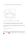
One of the datasets is Nile, containing data on the flow of the Nile River. Let’s again find the mean and
standard deviation,
> mean(Nile)
[1] 919.35
> sd(Nile)
[1] 169.2275
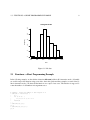
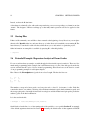
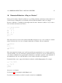
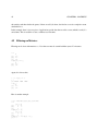
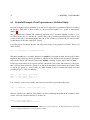
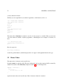
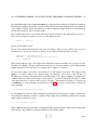
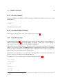
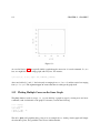
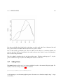
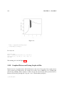
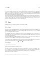
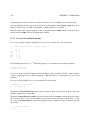
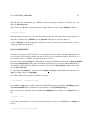
and also plot a histogram of the data:
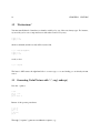
> hist(Nile)
A window pops up with the histogram in it, as seen in Figure 2.1. This one is bare-bones simple, but R has
all kinds of bells and whistles you can use optionally. For instance, you can change the number of bins by
specifying the breaks variable; hist(z,breaks=12) would draw a histogram of the data z with 12 bins. You
can make nicer labels, etc. When you become more familiar with R, you’ll be able to construct complex
color graphics of striking beauty.
Well, that’s the end of this first 5-minute introduction. We leave by calling the quit function (or optionally
by hitting ctrl-d in Linux):
> q()
Save workspace image? [y/n/c]: n
That last question asked whether we want to save our variables, etc., so that we can resume work later on.
If we answer y, then the next time we run R, all those objects will automatically be loaded. This is a very
important feature, especially when working with large or numerous datasets; see more in Section 2.7.
2.3. FUNCTIONS: A SHORT PROGRAMMING EXAMPLE
9
15
10
0
5
Frequency
20
25
Histogram of Nile
400
600
800
1000
1200
1400
Nile
Figure 2.1: Nile data
2.3
Functions: a Short Programming Example
In the following example, we first define a function oddcount() while in R’s interactive mode. (Normally
we would compose the function using a text editor, but in this quick-and-dirty example, we enter it line by
line in interactive mode.) We then call the function on a couple of test cases. The function is supposed to
count the number of odd numbers in its argument vector.
# comment: counts the number of odd integers in x
> oddcount <- function(x) {
+
k <- 0
+
for (n in x) {
+
if (n %% 2 == 1) k <- k+1
+
}
+
return(k)
+ }
> oddcount(c(1,3,5))
[1] 3
> oddcount(c(1,2,3,7,9))
[1] 4
10
CHAPTER 2. GETTING STARTED
Here is what happened: We first told R that we would define a function oddcount() of one argument x. The
left brace demarcates the start of the body of the function. We wrote one R statement per line. Since we
were still in the body of the function, R reminded us of that by using + as its prompt1 instead of the usual
>. After we finally entered a right brace to end the function body, R resumed the > prompt.
Note that arguments in R functions are read-only, in that a copy of the argument is made to a local variable,
and changes to the latter don’t affect the original variable. Thus changes to the original variable are typically
made by reassigning the return value of the function.
If one feels comfortable using global variables, a global can be written to from within a function, using R’s
superassignment operator, << −.
For instance:
> w <- 5
> addone <- function(x)
+
x <- x+1
> addone(w) # formal argument x is only a local copy of w
> w # so w doesn’t change
[1] 5
> addone <- function(x) return(x+1)
> w <- addone(w)
> w
[1] 6
> addone <- function() w <<- w+1 # use of superassignment op
> addone()
> w
[1] 7
Further details will be discussed in Chapter 8.
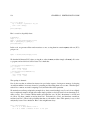
R also makes frequent use of default arguments. In the (partial) function definition
function(x,y=2)
y will be initialized to 2 if the programmer does not specify y in the call.
2.4
Preview of Some Important R Data Structures
Here we browse through some of the most frequently-used R data structures. This will give you a better
overview of R before diving into the details, and will also allow usage of these structures in examples without
having “forward references.”
1
Actually, this is a line continuation character.
2.4. PREVIEW OF SOME IMPORTANT R DATA STRUCTURES
2.4.1
11
Vectors
The vector type is the R workhorse. It’s hard to imagine R code, or even an R interactive session, that
doesn’t involve vectors.
Our examples of vectors in the preceding sessions will suffice for now.
2.4.2
Matrices
A matrix corresponds to the mathematical concept, i.e. a rectangular array. Technically, it is a vector, with
two attributes added—the numbers of rows and columns.
Here is some sample code:
> m <- rbind(c(1,4),c(2,2))
> m
[,1] [,2]
[1,]
1
4
[2,]
2
2
> m %*% c(1,1)
[,1]
[1,]
5
[2,]
4
First we used the rbind() (“row bind”) function to build a matrix from two vectors, storing the result in m.
We then typed that latter name, to confirm that we produced the intended matrix. Finally, we multiplied
the vector (5,4) by m. In order to get matrix multiplication of the mathematical type, we used the %*%
operator.
2.4.3
Lists
An R list is analogous to a C struct, i.e. a container whose contents can be items of diverse data types.
A common usage is to package the return values of elaborate statistical functions. For example, the lm()
(“linear model”) function performs regression analysis, computing not only the estimated coefficient but
also residuals, hypothesis test statistics and so on. These are packaged into a list, thus enabling a single
return value.
List members, which in C are delimited with periods, are indicated with dollar signs in R. Thus x$u is the u
component in the list x.
2.4.4
Data Frames
A typical data set contains data of diverse types, e.g. numerical and character string. So, while a data set
of, say, n observations of r variables has the “look and feel” of a matrix, it does not qualify as such in R.
12
CHAPTER 2. GETTING STARTED
Instead, we have the R data frame.
A data frame is technically a list, with each component being a vector corresponding to a column in our data
“matrix.” The designers of R have set things up so that many matrix operations can also be applied to data
frames.
2.5
Startup Files
If there are R commands you would like to have executed at the beginning of every R session, you can place
them in a file .Rprofile either in your home directory or in the directory from which you are running R. The
latter directory is searched for such a file first, which allows you to customize for a particular project.
Other information on startup files is available by querying R’s online help facility:
> ?.Rprofile
2.6
Extended Example: Regression Analysis of Exam Grades
For our second introductory example, we walk through a brief statistical regression analysis. There won’t be
much actual programming in this example, but it will illustrate usage of some of the data types from the last
section, will introduce R’s style of object-oriented programming, and will and serve as the basis for several
of our programming examples in subsequent chapters.
Here I have a file, ExamsQuiz.txt of grades from a class I taught. The first few lines are
2
3.3
4
2.3
...
3.3
2
4.3
0
4
3.7
4
3.3
The numbers correspond to letter grades on a four-point scale, so that 3.3, for instance, is a B+. Each line
contains the data for one student, consisting of the midterm examination grade, final examination grade, and
the average quiz grade. One might be interested in seeing how well the midterm and quiz grades predict the
student’s grade on the final examination.
Let’s first read in the file:
> examsquiz <- read.table("ExamsQuiz.txt",header=F)
Our file had no header line, i.e. no line naming each of the variables, so we specified header=F, an example
of the default arguments mentioned in Section 2.3. Actually, the default value of that argument is FALSE
2.6. EXTENDED EXAMPLE: REGRESSION ANALYSIS OF EXAM GRADES
13
anyway, as can be checked by R’s online help facility for read.table(). Thus we didn’t need to specify the
header argument, but it’s clearer if we do.
So, our data is now in examsquiz, an R object of class “data.frame”:
> class(examsquiz)
[1] "data.frame"
Just to check that the file was read in correctly, let’s take a look at the first few rows:
> head(examsquiz)
V1 V2 V3
1 2.0 3.3 4.0
2 3.3 2.0 3.7
3 4.0 4.3 4.0
4 2.3 0.0 3.3
5 2.3 1.0 3.3
6 3.3 3.7 4.0
Lacking a header for the data, R named the columns V1, V2 and V3. Row numbers appear on the left.
Let’s try to predict Exam 2 from Exam 1:
lma <- lm(examsquiz[,2] ˜ examsquiz[,1])
The lm() (“linear model”) function call here instructs R to fit the prediction equation
predicted Exam 2 = β0 + β1 Exam 1
(2.1)
using least squares. Note that Exam 1, being stored in column of our data frame, is referred to collectively
as examsquiz[,1]. Here the lack of the first subscript, i.e. row number, means that we are referring to the
entire column, and similarly for Exam 2.
The results are returned in the object we’ve named lma of class “lm”. We can see the various components
of that object by calling attributes():
> attributes(lma)
$names
[1] "coefficients" "residuals"
[5] "fitted.values" "assign"
[9] "xlevels"
"call"
"effects"
"qr"
"terms"
"rank"
"df.residual"
"model"
$class
[1] "lm"
For instance, the estimated values of the βi are stored in lma$coefficients. As usual, we can print them, by
typing the name, and by the way save some typing by abbreviating:
14
CHAPTER 2. GETTING STARTED
> lma$coef
(Intercept) examsquiz[, 1]
1.1205209
0.5899803
Since lma$coefficients is a vector, printing it is simple. But consider what happens when we print the object
lma itself:
> lma
Call:
lm(formula = examsquiz[, 2] ˜ examsquiz[, 1])
Coefficients:
(Intercept)
1.121
examsquiz[, 1]
0.590
How did R know to print only these items, and not the other components of lma? The answer is that the
generic function used for any printing, print(), actually hands off the work to a print function that has
been declared to be the one associated with objects of class “lm”. This function is named print.lm(), and
illustrates the concept of polymorphism we introduced briefly in Chapter 1. We’ll see the details in Chapter
12.
We can get a more detailed printout of the contents of lma by calling summary(), another generic function,
which in this case triggers a call to summary.lm() behind the scenes:
> summary(lma)
Call:
lm(formula = examsquiz[, 2] ˜ examsquiz[, 1])
Residuals:
Min
1Q
-3.4804 -0.1239
Median
0.3426
3Q
0.7261
Max
1.2225
Coefficients:
(Intercept)
examsquiz[, 1]
--Signif. codes:
Estimate Std. Error t value Pr(>|t|)
1.1205
0.6375
1.758 0.08709 .
0.5900
0.2030
2.907 0.00614 **
0 *** 0.001 ** 0.01 * 0.05 . 0.1
1
Residual standard error: 1.092 on 37 degrees of freedom
Multiple R-squared: 0.1859,
Adjusted R-squared: 0.1639
F-statistic: 8.449 on 1 and 37 DF, p-value: 0.006137
A number of other generic functions are defined for this class. See the online help for lm() for details.
To predict Exam 2 from both Exam 1 and the Quiz score, we would use the ‘+’ notaiton:
> lmb <- lm(examsquiz[,2] ˜ examsquiz[,1] + examsquiz[,3])
(There is also a ‘*’ notation, not covered here.)
2.7. SESSION DATA
2.7
15
Session Data
As you proceed through an interactive R session, R will record the commands you submit. And as you long
as you answer yes to the question “Save workspace image?” put to you when you quit the session, R will
save all the objects you created in that session, and restore them in your next session. You thus do not have
to recreate the objects again from scratch if you wish to continue work from before.
The saved workspace file is named .Rdata, and is located either in the directory from which you invoked
this R session (Linux) or in the R installation directory (Windows). Note that that means that in Windows, if
you use R from various different directories, each save operation will overwrite the last. That makes Linux
more convenient, but note that the file can be quite voluminous, so be sure to delete it if you are no longer
working on that particular project.
You can also save the image yourself, to whatever file you wish, by calling save.image(). You can restore
the workspace from that file later on by calling load().
16
CHAPTER 2. GETTING STARTED
Chapter 3
Vectors
The fundamental data type in R is, without question, the vector. You’ll learn all about vectors in this chapter.
3.1
Scalars, Vectors, Arrays and Matrices
Remember, objects are actually considered one-element vectors. So, there is really no such thing as a scalar.
Vector elements must all have the same mode, which can be integer, numeric (floating-point number),
character (string), logical (boolean), complex, object, etc.
Vectors indices begin at 1. Note that vectors are stored like arrays in C, i.e. contiguously, and thus one
cannot insert or delete elements, a la Python. If you wish to do this, use a list instead.
A variable might not have a value, a situation designated as NA. This is like None in Python and undefined
in Perl, though its origin is different. In statistical datasets, one often encounters missing data, i.e. observations for which the values are missing. In many of R’s statistical functions, we can instruct the function to
skip over any missing values.
Arrays and matrices are actually vectors too, as you’ll see; they merely have extra attributes, e.g. in the
matrix case the numbers of rows and columns. Keep in mind that since arrays and matrices are vectors, that
means that everything we say about vectors applies to them too.
One can obtain the length of a vector by using the function of the same name, e.g.
> x <- c(1,2,4)
> length(x)
[1] 3
17
18
3.2
CHAPTER 3. VECTORS
“Declarations”
You must warn R ahead of time that you intend a variable to be one of the vector/array types. For instance,
say we wish y to be a two-component vector with values 5 and 12. If you try
> y[1] <- 5
> y[2] <- 12
the first command (and the second) will be rejected, but
> y <- vector(length=2)
> y[1] <- 5
> y[2] <- 12
works, as does
> y <- c(5,12)
The latter is OK because the right-hand side is a vector type, so we are binding y to an already-existent
vector.
3.3
Generating Useful Vectors with “:”, seq() and rep()
Note the : operator:
> 5:8
[1] 5 6 7 8
> 5:1
[1] 5 4 3 2 1
Beware of the operator precedence:
> i <- 2
> 1:i-1
[1] 0 1
> 1:(i-1)
[1] 1
The seq() (”sequence”) generates an arithmetic sequence, e.g.:
3.4. VECTOR ARITHMETIC AND LOGICAL OPERATIONS
19
> seq(5,8)
[1] 5 6 7 8
> seq(12,30,3)
[1] 12 15 18 21 24 27 30
> seq(1.1,2,length=10)
[1] 1.1 1.2 1.3 1.4 1.5 1.6 1.7 1.8 1.9 2.0
Though it may seem innocuous, the seq() function provides foundation for many R operations. See examples
in Sections 10.8 and Section 13.16.
The rep() (”repeat”) function allows us to conveniently put the same constant into long vectors. The call
form is rep(z,k), which creates a vector of k*length(z) elements, each equal to z. For example:
> x <- rep(8,4)
> x
[1] 8 8 8 8
> rep(1:3,2)
[1] 1 2 3 1 2 3
3.4
Vector Arithmetic and Logical Operations
You can add vectors, e.g.
> x <- c(1,2,4)
> x + c(5,0,-1)
[1] 6 2 3
You may surprised at what happens when we multiply them:
> x * c(5,0,-1)
[1] 5 0 -4
As you can see, the multiplication was elementwise. This is due to the functional programming nature of R.
The any() and all() functions are handy:
> x <- 1:10
> if (any(x
[1] "yes"
> if (any(x
> if (all(x
> if (all(x
[1] "yes"
> 8)) print("yes")
> 88)) print("yes")
> 88)) print("yes")
> 0)) print("yes")
20
3.5
CHAPTER 3. VECTORS
Recycling
When applying an operation to two vectors which requires them to be the same length, the shorter one will
be recycled, i.e. repeated, until it is long enough to match the longer one, e.g.
> c(1,2,4) + c(6,0,9,20,22)
[1] 7 2 13 21 24
Warning message:
longer object length
is not a multiple of shorter object length in: c(1, 2, 4) + c(6,
0, 9, 20, 22)
Here’s a more subtle example:
> x
[,1] [,2]
[1,]
1
4
[2,]
2
5
[3,]
3
6
> x+c(1,2)
[,1] [,2]
[1,]
2
6
[2,]
4
6
[3,]
4
8
What happened here is that x, as a 3x2 matrix, is also a six-element vector, which in R is stored column-bycolumn. We added a two-element vector to it, so our addend had to be repeated twice to make six elements.
So, we were adding c(1,2,1,2,1,2) to x.
3.6
Vector Indexing
You can also do indexing of vectors, picking out elements with specific indices, e.g.
> y <- c(1.2,3.9,0.4,0.12)
> y[c(1,3)]
[1] 1.2 0.4
> y[2:3]
[1] 3.9 0.4
Note carefully that duplicates are definitely allowed, e.g.
> x <- c(4,2,17,5)
> y <- x[c(1,1,3)]
> y
[1] 4 4 17
3.7. VECTOR ELEMENT NAMES
21
Negative subscripts mean that we want to exclude the given elements in our output:
> z <- c(5,12,13)
> z[-1] # exclude element 1
[1] 12 13
> z[-1:-2]
[1] 13
In such contexts, it is often useful to use the length() function:
> z <- c(5,12,13)
> z[1:length(z)-1]
[1] 5 12
Note that this is more general than using z[1:2]. In a program with general-length vectors, we could use this
pattern to exclude the last element of a vector.
Here is a more involved example of this principle. Suppose we have a sequence of numbers for which we
want to find successive differences, i.e. the difference between each number and its predecessor. Here’s how
we could do it:
> x <- c(12,15,8,11,24)
> y <- x[-1] - x[-length(x)]
> y
[1] 3 -7 3 13
Here we want to find the numbers 15-12 = 3, 8-15 = -7, etc. The expression x[-1] gave us the vector
(15,8,11,24) and x[-length(x)] gave us (12,15,8,11). Subtracting these two vectors then gave us the differences we wanted.
Make careful note of the above example. This is the “R way of doing things.” By taking advantage
of R’s vector operations, we came up with a solution which avoids loops. This is clean, compact and
likely much faster when our vectors are long. We often use R’s functional programming features to
these ends as well.
3.7
Vector Element Names
The elements of a vector can optionally be given names. For instance:
> x <- c(1,2,4)
> names(x)
NULL
> names(x) <- c("a","b","ab")
> names(x)
[1] "a" "b" "ab"
> x
a b ab
1 2 4
22
CHAPTER 3. VECTORS
We can remove the names from a vector by assigning NULL:
> names(x) <- NULL
> x
[1] 1 2 4
We can even reference elements of the vector by name, e.g.
> x <- c(1,2,4)
> names(x) <- c("a","b","ab")
> x["b"]
b
2
3.8
Elementwise Operations on Vectors
Suppose we have a function f() that we wish to apply to all elements of a vector x. In many cases, we can
accomplish this by simply calling f() on x itself.
3.8.1
Vectorized Functions
As we saw in Section 3.4, many operations are vectorized, such as + and >:
> u <- c(5,2,8)
> v <- c(1,3,9)
> u+v
[1] 6 5 17
> u > v
[1] TRUE FALSE FALSE
The key point is that if an R function uses vectorized operations, it too is vectorized, i.e. it can be applied to
vectors in an elementwise fashion. For instance:
> w <- function(x) return(x+1)
> w(u)
[1] 6 3 9
Here w() uses +, which is vectorized, so w() is vectorized as well.
The function can have auxiliary arguments:
> f
function(x,c) return((x+c)ˆ2)
> f(1:3,0)
[1] 1 4 9
> f(1:3,1)
[1] 4 9 16
3.8. ELEMENTWISE OPERATIONS ON VECTORS
23
Even the transcendental functions are vectorized:
> sqrt(1:9)
[1] 1.000000 1.414214 1.732051 2.000000 2.236068 2.449490 2.645751 2.828427
[9] 3.000000
This applies to many of R’s built-in functions. For instance, let’s apply the function for rounding to the
nearest integer to an example vector y:
> y <- c(1.2,3.9,0.4)
> z <- round(y)
> z
[1] 1 4 0
The point is that the round() function was applied individually to each element in the vector y. In fact, in
> round(1.2)
[1] 1
the operation still works, because the number 1.2 is actually considered to be a vector that happens to consist
of a single element 1.2.
Here we used the built-in function round(), but you can do the same thing with functions that you write
yourself.
Note that the functions can also have extra arguments, e.g.
> f <- function(elt,s) return(elt+s)
> y <- c(1,2,4)
> f(y,1)
[1] 2 3 5
As seen above, even operators such as + are really functions. For example, the reason why elementwise
addition of 4 works here,
> y <- c(12,5,13)
> y+4
[1] 16 9 17
is that the + is actually considered a function! Look at it here:
> ’+’(y,4)
[1] 16 9 17
24
3.8.2
CHAPTER 3. VECTORS
The Case of Vector-Valued Functions
The above operations work with vector-valued functions too. However, since the return value is in essence
a matrix, it needs to be converted. A better option is to use sapply(), discussed in Section 4.10.2.
3.8.3
Elementwise Operations in Nonvectorizable Settings
Even if a function that you want to apply to all elements of a vector is not vectorizable, you can still avoid
writing a loop, e.g. avoid writing
lv <- length(v)
outvec <- vector(length=lv)
for (i in 1:lv) {
outvec[i] <- f(v[i])
}
by treating the vector as a matrix and using the apply() function (Section 4.10:
outvec <- apply(as.matrix(v),1,f)
The call to as.matrix() will return a matrix whose sole column is v.
This may not save you much time if you are running R on just one machine, but if you are using, for instance,
the snow package (see Section 17.3), with parApply() instead of apply(), it could be well worth doing.
3.9
Filtering
Another idea borrowed from functional programming is filtering, which is one of the most common operations in R.
For example:
> z <- c(5,2,-3,8)
> w <- z[z*z > 8]
> w
[1] 5 -3 8
Here is what happened above: We asked R to find the indices of all the elements of z whose squares were
greater than 8, then use those indices in an indexing operation on z, then finally assign the result to w.
Look at it done piece-by-piece:
3.9. FILTERING
> z <- c(5,2,-3,8)
> z
[1] 5 2 -3 8
> z*z > 8
[1] TRUE FALSE TRUE
25
TRUE
Evaluation of the expression z*z > 8 gave us a vector of booleans! Let’s go further:
> z[c(TRUE,FALSE,TRUE,TRUE)]
[1] 5 -3 8
This example will place things into even sharper focus:
> z <- c(5,2,-3,8)
> j <- z*z > 8
> j
[1] TRUE FALSE TRUE
> y <- c(1,2,30,5)
> y[j]
[1] 1 30 5
TRUE
We may just want to find the positions within z at which the condition occurs. We can do this using which():
> which(z*z > 8)
[1] 1 3 4
Here’s an extension of an example in Section 3.6:
# x is an array of numbers, mostly in nondecreasing order, but with some
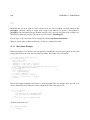
# violations of that order nviol() returns the number of indices i for
# which x[i+1] < x[i]
nviol <- function(x) {
diff <- x[-1]-x[1:(length(x)-1)]
return(length(which(diff < 0)))
}
I noted in Section 1.2 that using the nrow() function in conjunction with filtering provides a way to obtain
a count of records satisfying various conditions. If you just want the count and don’t want to create a new
table, you should use this approach.
You can also use this to selectively change elements of a vector, e.g.
> x <- c(1,3,8,2)
> x[x > 3] <- 0
> x
[1] 1 3 0 2
26
3.10
CHAPTER 3. VECTORS
Combining Elementwise Operations and Filtering, with the ifelse() Function
The form is
ifelse(b,u,v)
where b is a boolean vector, and u and v are vectors.
The return value is a vector, element i of which is u[i] if b[i] is true, or v[i] if b[i] is false. This is pretty
abstract, so let’s go right to an example:
> x <- 1:10
> y <- ifelse(x %% 2 == 0,5,12)
> y
[1] 12 5 12 5 12 5 12 5 12
5
Here we wish to produce a vector in which there is a 5 wherever x is even, with a 12 wherever x is odd.
So, the first argument is c(F,T,F,T,F,T,F,T,F,T). The second argument, 5, is treated as c(5,5,5,5,5,5,5,5,5,5)
by recycling, and similarly for the third argument.
Here is another example, in which we have explicit vectors.
> x <- c(5,2,9,12)
> ifelse(x > 6,2*x,3*x)
[1] 15 6 18 24
The advantage of ifelse() over the standard if-then-else is that it is vectorized. Thus it’s potentially much
faster.
3.11
Extended Example: Recoding an Abalone Data Set
Due to the vector nature of the arguments, one can nest ifelse() operations. In the following example,
involving an abalone data set, gender is coded as ‘M’, ‘F’ or ‘I’, the last meaning infant. We wish to recode
those characters as 1, 2 or 3:
> g <- c("M","F","F","I","M")
> ifelse(g == "M",1,ifelse(g == "F",2,3))
[1] 1 2 2 3 1
The inner call to ifelse(), which of course is evaluated first, produces a vector of 2s and 3s, with the 2s
corresponding to female cases, and 3s being for males and infants. The outer call results in 1s for the males,
in which cases the 3s are ignored.
3.11. EXTENDED EXAMPLE: RECODING AN ABALONE DATA SET
27
Remember, the vectors involved could be columns in matrices, and this is a very common scenario. Say our
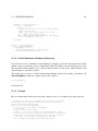
abalone data is stored in the matrix ab, with gender in the first column. Then if we wish to recode as above,
we could do it this way:
> ab[,1] <- ifelse(ab[,1] == "M",1,ifelse(ab[,1] == "F",2,3))
28
CHAPTER 3. VECTORS
Chapter 4
Matrices
A matrix is a vector with two additional attributes, the number of rows and number of columns.
4.1
General Operations
Multidimensional vectors in R are called arrays. A two-dimensional array is also called a matrix, and is
eligible for the usual matrix mathematical operations.
Matrix row and column subscripts begin with 1, so for instance the upper-left corner of the matrix a is
denoted a[1,1]. The internal linear storage of a matrix is in column-major order, meaning that first all of
column 1 is stored, then all of column 2, etc.
One of the ways to create a matrix is via the matrix() function, e.g.
> y <- matrix(c(1,2,3,4),nrow=2,ncol=2)
> y
[,1] [,2]
[1,] 1
3
[2,] 2
4
Here we concatenated what we intended as the first column, the numbers 1 and 2, with what we intended as
the second column, 3 and 4. That was our data in linear form, and then we specified the number of rows and
columns. The fact that R uses column-major order then determined where these four numbers were put.
Though internal storage of a matrix is in column-major order, we can use the byrow argument in matrix()
to TRUE in order to specify that the data we are using to fill a matrix be interpreted as being in row-major
order. For example:
> m <- matrix(c(1,2,3,4,5,6),nrow=3)
> m
29
30
CHAPTER 4. MATRICES
[,1] [,2]
[1,]
1
4
[2,]
2
5
[3,]
3
6
> m <- matrix(c(1,2,3,4,5,6),nrow=2,byrow=T)
> m
[,1] [,2] [,3]
[1,]
1
2
3
[2,]
4
5
6
(‘T’ is an abbreviation for “TRUE”.)
Since we specified the matrix entries in the above example, we would not have needed to specify ncol; just
nrow would be enough. For instance:
> y <- matrix(c(1,2,3,4),nrow=2)
> y
[,1] [,2]
[1,] 1
3
[2,] 2
4
Note that when we then printed out y, R showed us its notation for rows and columns. For instance, [,2]
means column 2, as can be seen in this check:
> y[,2]
[1] 3 4
Another way we could have built y would have been to specify elements individually:
>
>
>
>
>
>
y <- matrix(nrow=2,ncol=2)
y[1,1] = 1
y[2,1] = 2
y[1,2] = 3
y[2,2] = 4
y
[,1] [,2]
[1,] 1
3
[2,] 2
4
We can perform various operations on matrices, e.g. matrix multiplication, matrix scalar multiplication and
matrix addition:
> y %*% y # ordinary matrix multiplication
[,1] [,2]
[1,] 7
15
[2,]10
22
> 3*y
[,1] [,2]
[1,] 3
9
[2,] 6
12
4.2. MATRIX INDEXING
31
> y+y
[,1] [,2]
[1,] 2
6
[2,] 4
8
For linear algebra operations on matrices, see Section 10.4.
Again, keep in mind—and when possible, exploit—the notion of recycling (Section 3.5. For instance:
> x <- 1:2
> y <- c(1,3,4,10)
> x*y
[1] 1 6 4 20
Since x was shorter than y, it was recycled to the four-element vector c(1,2,1,2), then multiplied elementwise
with y.
4.2
Matrix Indexing
The same operations we discussed in Section 3.6 apply to matrices. For instance:
> z
[,1] [,2] [,3]
[1,] 1
1
1
[2,] 2
1
0
[3,] 3
0
1
[4,] 4
0
0
> z[,c(2,3)]
[,1] [,2]
[1,] 1
1
[2,] 1
0
[3,] 0
1
[4,] 0
0
Here’s another example:
> y <- matrix(c(11,21,31,12,22,32),nrow=3,ncol=2)
> y
[,1] [,2]
[1,]11
12
[2,]21
22
[3,]31
32
> y[2:3,]
[,1] [,2]
[1,]21
22
[2,]31
32
> y[2:3,2]
[1] 22 32
32
CHAPTER 4. MATRICES
You can copy a smaller matrix to a slice of a larger one:
> y
[,1] [,2]
[1,]
1
4
[2,]
2
5
[3,]
3
6
> y[2:3,] <- matrix(c(1,1,8,12),nrow=2)
> y
[,1] [,2]
[1,]
1
4
[2,]
1
8
[3,]
1
12
> x <- matrix(nrow=3,ncol=3)
> x[2:3,2:3] <- cbind(4:5,2:3)
> x
[,1] [,2] [,3]
[1,]
NA
NA
NA
[2,]
NA
4
2
[3,]
NA
5
3
4.3
Matrix Row and Column Mean Functions
The function mean() applies only to vectors, not matrices. If one does call this function with a matrix argument, the mean of all of its elements is computed, not multiple means row-by-row or column-by-column,
since a matrix is a vector.
The functions rowMeans() and colMeans() return vectors containing the means of the rows and columns.
There are also corresponding functions rowSums() and colSums().
4.4
Matrix Row and Column Names
The natural way to refer to rows and columns in a matrix is, of course, via the row and column numbers.
However, optionally one can give alternate names to these entities.
For example:
> z <- matrix(c(1,2,3,4),nrow=2)
> z
[,1] [,2]
[1,]
1
3
[2,]
2
4
> colnames(z)
NULL
> colnames(z) <- c("a","b")
> z
a b
4.5. EXTENDED EXAMPLE: PRELIMINARY ANALYSIS OF AUTOMOBILE DATA
33
[1,] 1 3
[2,] 2 4
> colnames(z)
[1] "a" "b"
> z[,"a"]
[1] 1 2
As you see here, these names can then be used to reference specific columns. The function rownames()
works similarly.
This feature is usually less important when writing R code for general application, but can be very useful
when analyzing a specific data set. An example of this is seen in Section 4.5.
4.5
Extended Example: Preliminary Analysis of Automobile Data
Here we look at one of R’s built-in data sets, named mtcars, automobile data collected back in 1974. The
help file for this data set is invoked as usual via
> ?mtcars
while the data set itself, being in the form of a data frame, is accessed simply by its name.
There are data on 11 variables, as the help file tells us:
[, 1]
[, 2]
[, 3]
[, 4]
[, 5]
[, 6]
[, 7]
[, 8]
[, 9]
[,10]
[,11]
mpg
cyl
disp
hp
drat
wt
qsec
vs
am
gear
carb
Miles/(US) gallon
Number of cylinders
Displacement (cu.in.)
Gross horsepower
Rear axle ratio
Weight (lb/1000)
1/4 mile time
V/S
Transmission (0 = automatic, 1 = manual)
Number of forward gears
Number of carburetors
Since this chapter concerns matrix objects, let us first change it to a matrix. This is not really necessary in
this case, as the matrix indexing operations we’ve covered here do apply to data frames too, but it’s important
to understand that these are two different classes. Here is how we do the conversion:
> class(mtcars)
[1] "data.frame"
> mtc <- mtcars
> class(mtc)
[1] "data.frame"
Let’s take a look at the first few records, i.e. the first few rows:
34
CHAPTER 4. MATRICES
> head(mtc)
Mazda RX4
Mazda RX4 Wag
Datsun 710
Hornet 4 Drive
Hornet Sportabout
Valiant
mpg cyl disp hp drat
wt qsec vs am gear carb
21.0
6 160 110 3.90 2.620 16.46 0 1
4
4
21.0
6 160 110 3.90 2.875 17.02 0 1
4
4
22.8
4 108 93 3.85 2.320 18.61 1 1
4
1
21.4
6 258 110 3.08 3.215 19.44 1 0
3
1
18.7
8 360 175 3.15 3.440 17.02 0 0
3
2
18.1
6 225 105 2.76 3.460 20.22 1 0
3
1
You can see that the matrix has been given row names corresponding to the car names. The columns have
names too.
Let’s find the overall average mile-per-gallon figure:
> mean(mtc[,1])
[1] 20.09062
Now let’s break it down by number of cylinders:
> mean(mtc[mtc[,2] == 4,1])
[1] 26.66364
> mean(mtc[mtc[,2] == 6,1])
[1] 19.74286
> mean(mtc[mtc[,2] == 8,1])
[1] 15.1
Or, more compactly from a programming point of view:
> for (ncyl in c(4,6,8)) print(mean(mtc[mtc[,2] == ncyl,1]))
[1] 26.66364
[1] 19.74286
[1] 15.1
As explained earlier, here the expression mtc[,2] == ncyl returns a boolean vector, with TRUE components corresponding to the rows in mtc that satisfy mtc[,2] == ncyl. The expression mtc[mtc[,2] ==
ncy,1] yields a submatrix consisting of those rows of mtc, in which we look at column 1.
How many have more than 200 horsepower? Which are they?
> nrow(mtc[mtc[,4] > 200,])
[1] 7
> rownames(mtc[mtc[,4] > 200,])
[1] "Duster 360"
"Cadillac Fleetwood"
[4] "Chrysler Imperial"
"Camaro Z28"
[7] "Maserati Bora"
"Lincoln Continental"
"Ford Pantera L"
As can be seen in the first command above, the nrow() function is a handy way to find the count of the number of rows satisfying a certain condition. In the second command, we extracted a submatrix corresponding
to the given condition, and then asked for the names of the rows of that submatrix—giving us the names of
the cars satisfying the condition.
4.6. DIMENSION REDUCTION: A BUG OR A FEATURE?
4.6
35
Dimension Reduction: a Bug or a Feature?
In the world of statistics, dimension reduction is a good thing, with many statistical procedures aimed to do
it well. If we are working with, say, 10 variables, and can reduce that number to three, we’re happy.
However, in R there is something else that might merit the name “dimension reduction. Say we have a
four-row matrix, and extract a row from it:
> z <- matrix(1:8,nrow=4)
> z
[,1] [,2]
[1,]
1
5
[2,]
2
6
[3,]
3
7
[4,]
4
8
> r <- z[2,]
> r
[1] 2 6
This seems innocuous, but note the format in which R has displayed r. It’s a vector format, not a matrix
format. In other words, r is a vector of length 2, rather than a 1x2 matrix. We can confirm this:
> attributes(z)
$dim
[1] 4 2
> attributes(r)
NULL
This seems natural, but in many cases it will cause trouble in programs that do a lot of matrix operations.
You may find that your code works fine in general, but fails in a special case. Say for instance that your
code extracts a submatrix from a given matrix, and then does some matrix operations on the submatrix. If
the submatrix has only one row, R will make it a vector, which could ruin your computation.
Fortunately, R has a way to suppress this dimension reduction, with the drop argument. For example:
> r <- z[2,, drop=F]
> r
[,1] [,2]
[1,]
2
6
> dim(r)
[1] 1 2
Ah, now r is a 1x2 matrix.
See Sections 4.8 for an example in which drop is used.
If you have a vector which you wish to be treated as a matrix, use as.matrix():
36
CHAPTER 4. MATRICES
> u
[1] 1 2 3
> v <- as.matrix(u)
> attributes(u)
NULL
> attributes(v)
$dim
[1] 3 1
4.7
Adding/Deleting Elements of Vectors and Matrices
Technically, vectors and matrices are of fixed length and dimensions. However, they can be reassigned, etc.
Consider:
> x
> x
> x
[1]
> x
> x
[1]
> x
> x
[1]
<- c(12,5,13,16,8)
<- c(x,20) # append 20
12 5 13 16 8 20
<- c(x[1:3],20,x[4:6])
12 5 13 20 16
<- x[-2:-4]
12 16
8 20
# insert 20
# delete elements 2 through 4
8 20
The rbind() and cbind() functions enable one to add rows or columns to a matrix.
For example:
> one
[1] 1 1 1 1
> z
[,1] [,2] [,3]
[1,] 1
1
1
[2,] 2
1
0
[3,] 3
0
1
[4,] 4
0
0
> cbind(one,z)
[1,]1 1 1 1
[2,]1 2 1 0
[3,]1 3 0 1
[4,]1 4 0 0
You can also use these functions as a quick way to create small matrices:
> q <- cbind(c(1,2),c(3,4))
> q
[,1] [,2]
[1,]
1
3
[2,]
2
4
4.8. EXTENDED EXAMPLE: DISCRETE-EVENT SIMULATION IN R
37
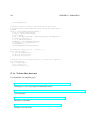
We can delete rows or columns in the same manner as shown for vectors above, e.g.:
> m <- matrix(1:6,nrow=3)
> m
[,1] [,2]
[1,]
1
4
[2,]
2
5
[3,]
3
6
> m <- m[c(1,3),]
> m
[,1] [,2]
[1,]
1
4
[2,]
3
6
4.8
Extended Example: Discrete-Event Simulation in R
Discrete-event simulation (DES) is widely used in business, industry and government. The term “discrete
event” refers to the fact that the state of the system changes only at discrete times, rather than changing
continuously. A typical example would involve a queuing system, say people lining up to use an ATM
machine. The number of people in the queue increases only when someone arrives, and decreases only
when a person finishes an ATM transaction, both of which occur only at discrete times.
It is not assumed here that the reader has prior background in DES. For our purposes here, the main ingredient to understand is the event list, which will now be explained.
Central to DES operation is maintenance of the event list, a list of scheduled events. Since the earliest event
must always be handled next, the event list is usually implemented as some kind of priority queue. The
main loop of the simulation repeatedly iterates, in each iteration pulling the earliest event off of the event
list, updating the simulated time to reflect the occurrence of that event, and reacting to this event. The latter
action will typically result in the creation of new events. R’s lack of pointer variables means that we must
write code for maintaining the event list in a nontraditional way, but on the other hand it will also lead to
some conveniences too.
One of the oldest approaches to write DES code is the event-oriented paradigm. Here the code to handle the
occurrence of one event sets up another event. In the case of an arrival to a queue, the code may then set up
a service event (or, if there are queued jobs, it will add this job to the queue). As an example to guide our
thinking, consider the ATM situation, and suppose we store the event list as a simple vector.
At time 0, the queue is empty. The simulation code randomly generates the time of the first arrival, say 2.3.
At this point the event list is simply (2.3). This event is pulled off the list, simulated time is updated to 2.3,
and we react to the arrival event as follows: The queue for the ATM is empty, so we start the service, by
randomly generating the service time; say it is 1.2 time units. Then the completion of service will occur at
simulated time 2.3+1.2 = 3.5, so we add this event to the event list, which will now consist of (3.5). We will
also generate the time to the next arrival, say 0.6, which means the arrival will occur at time 2.9. Now the
event list consists of (2.9,3.5).
38
CHAPTER 4. MATRICES
As will be detailed below, our example code here is hardly optimal, and the reader is invited to improve
it. It does, however, serve to illustrate a number of the issues we have discussed in this chapter. the code
consists of some generally-applicable library functions, such as schedevnt() and mainloop(), and a sample
application of those library functions. The latter simulates an M/M/1 queue, i.e. a single-server queue in
which both interarrival time and service time are exponentially distributed.
1
# DES.r:
R routines for discrete-event simulation (DES), with an example
2
3
4
5
6
#
#
#
#
each event will be represented by a vector; the first component will
be the time the event is to occur; the second component will be the
numerical code for the programmer-defined event type; the programmer
may add application-specific components
7
8
9
10
# a list named "sim" holds the events list and other information; for
# convenience, sim has been stored as a global variable; some functions
# have side effects
11
12
13
14
15
16
17
# create "sim"
newsim <- function(numfields) {
sim <<- list()
sim$currtime <<- 0.0 # current simulated time
sim$evnts <<- NULL # event list
}
18
19
20
21
22
23
24
25
26
27
28
29
30
31
32
33
# insert event evnt into event list
insevnt <- function(evnt) {
if (is.null(sim$evnts)) {
sim$evnts <<- matrix(evnt,nrow=1)
return()
}
# find insertion point
inspt <- binsearch(sim$evnts[,1],evnt[1])
# now "insert"
if (inspt > 1) e <- rbind(sim$evnts[1:(inspt-1),],evnt)
nrse <- nrow(sim$evnts)
if (inspt <= nrse)
e <- rbind(evnt, sim$evnts[inspt:nrse,])
sim$evnts <<- e
}
34
35
36
37
38
39
40
41
# schedule new event; evnttime is the time at which the event is to
# occur; evnttype is the event type; and appfields are the values of the
# programmer-defined fields, if any
schedevnt <- function(evnttime,evnttype,appfields=NULL) {
evnt <- c(evnttime,evnttype,appfields)
insevnt(evnt)
}
42
43
44
45
46
47
48
49
50
51
52
# start to process next event (second half done by application
# programmer via call to reactevnt())
getnextevnt <- function() {
head <- sim$evnts[1,]
# delete head
if (nrow(sim$evnts) == 1) sim$evnts <<- NULL else
sim$evnts <<- sim$evnts[-1,,drop=F]
return(head)
}
4.8. EXTENDED EXAMPLE: DISCRETE-EVENT SIMULATION IN R
53
54
55
56
57
58
59
60
# main loop of the simulation
mainloop <- function(maxsimtime) {
while(sim$currtime < maxsimtime) {
head <- getnextevnt()
sim$currtime <<- head[1] # update current simulated time
reactevnt(head) # process this event (programmer-supplied ftn)
}
}
61
62
63
64
65
66
67
68
69
70
71
72
73
74
75
76
77
# binary search of insertion point of y in the sorted vector x; returns
# the position in x before which y should be inserted, with the value
# length(x)+1 if y is larger than x[length(x)]
binsearch <- function(x,y) {
n <- length(x)
lo <- 1
hi <- n
while(lo+1 < hi) {
mid <- floor((lo+hi)/2)
if (y == x[mid]) return(mid)
if (y < x[mid]) hi <- mid else lo <- mid
}
if (y <= x[lo]) return(lo)
if (y < x[hi]) return(hi)
return(hi+1)
}
78
79
# application:
M/M/1 queue, arrival rate 0.5, service rate 1.0
80
81
82
83
84
85
86
87
88
89
90
91
92
# globals
# rates
arvrate <- 0.5
srvrate <- 1.0
# event types
arvtype <- 1
srvdonetype <- 2
# initialize server queue
srvq <- NULL # will just consist of arrival times of queued jobs
# statistics
njobsdone <- NULL # jobs done so far
totwait <- NULL # total wait time so far
93
94
95
96
97
98
99
100
101
102
103
104
105
106
107
108
109
110
111
112
# event processing function requried by general DES code above
reactevnt <- function(head) {
if (head[2] == arvtype) { # arrival
# if server free, start service, else add to queue
if (length(srvq) == 0) {
srvq <<- head[3]
srvdonetime <- sim$currtime + rexp(1,srvrate)
schedevnt(srvdonetime,srvdonetype,head[3])
} else srvq <<- c(srvq,head[3])
# generate next arrival
arvtime <- sim$currtime + rexp(1,arvrate)
schedevnt(arvtime,arvtype,arvtime)
} else { # service done
# process job that just finished
# do accounting
njobsdone <<- njobsdone + 1
totwait <<- totwait + sim$currtime - head[3]
# remove from queue
srvq <<- srvq[-1]
39
40
CHAPTER 4. MATRICES
# more still in the queue?
if (length(srvq) > 0) {
# schedule new service
srvdonetime <- sim$currtime + rexp(1,srvrate)
schedevnt(srvdonetime,srvdonetype,srvq[1])
}
113
114
115
116
117
118
}
119
120
}
121
122
123
124
125
126
127
128
129
130
131
132
133
mm1sim <- function() {
srvq <<- vector(length=0)
njobsdone <<- 0
totwait <<- 0.0
# create simulation, 1 extra field (arrival time)
newsim(1)
# get things going, with first arrival event
arvtime <- rexp(1,rate=arvrate)
schedevnt(arvtime,arvtype,arvtime)
mainloop(100000.0)
return(totwait/njobsdone)
}
The simulation state, consisting of the current simulated time and the event list, have been placed in an R
list, sim. This was done out of a desire to encapsulate the information, which in R typically means using a
list.
This list sim has been made a global variable, for convenience and clarity. This has led to the use of R’s
superassignment operator << −, with associated side effects. For instance in mainloop(), the line
sim$currtime <<- head[1]
# update current simulated time
changes a global directly, while sim$evnts is changed indirectly via the call
head <- getnextevnt()
If one has objections to use of globals, this could be changed, though without pointers it could be done only
in a limited manner.
As noted, a key issue in writing a DES library is the event list. It has been implemented here as a matrix,
sim$evnts. Each row of the matrix corresponds to one scheduled event, with information on the event time,
the event type (say arrival or service completion) and any application-specific data the programmer wishes
to add. The rows of the matrix are in ascending order of event time, which is contained in the first column.
The main potential advantage of using a matrix as our structure here is that it enables us to maintain the
event list in ascending order by time via a binary search operation by event time in that first column. This is
done in the line
inspt <- binsearch(sim$evnts[,1],evnt[1])
4.8. EXTENDED EXAMPLE: DISCRETE-EVENT SIMULATION IN R
41
in insevnt(). Here we wish to insert a newly-created event into the event list, and the fact that we are working
with a vector enables the use of a fast binary search.
However, looks are somewhat deceiving here. Though for an event set of size n, the search will be of time
order O(log n), we still need O(n) to reassign the matrix, in the code
if (inspt > 1) e <- rbind(sim$evnts[1:(inspt-1),],evnt)
nrse <- nrow(sim$evnts)
if (inspt <= nrse)
e <- rbind(evnt, sim$evnts[inspt:nrse,])
sim$evnts <<- e
Again, this exemplifies the effects of lack of pointers. Here is a situation in which it may be useful to write
some code in C/C++ and then interface to R, which is discussed in Chapter 16.
This code above is a good example of the use of rbind(). We use the function to build up the new version
of sim$evnts with our new event inserted, row by row. Recall that in this matrix, earlier events are stored in
rows above later events. We first use rbind() to put together our new event with the existing events that are
earlier than it, if any:
if (inspt > 1) e <- rbind(sim$evnts[1:(inspt-1),],evnt)
Then, unless our new event is later than all the existing ones, we tack on the events that are later than it:
nrse <- nrow(sim$evnts)
if (inspt <= nrse)
e <- rbind(evnt, sim$evnts[inspt:nrse,])
There are a couple of items worth mentioning in the line
sim$evnts <<- sim$evnts[-1,,drop=F]
First, note that the negative-subscript feature of vector operations, in which the indices indicate which elements to skip, applies to matrices too. Here we are in essence deleting the first row of sim$evnts.
Second, here is an example of the need for drop. If there are just two events, the deletion will leave us with
only one. Without drop, the assignment would then change sim$evnts from a matrix to a vector, causing
problems in subsequent code that assumes it is a matrix.
The DES library code we’ve written above requires that the user provide a function reactevnt() that takes
the proper actions for each event. In our M/M/1 queue example here, we’ve defined two types of events—
arrival and service completion. Our function reactevnt() must then supply code to execute for each of these
two events. As mentioned earlier, for an arrival event, we must add the new job to the queue, and if the
server is idle, schedule a service event for this job. If a service completion event occurs, our code updates
42
CHAPTER 4. MATRICES
the statistics and then checks the queue; if there are still jobs there, the first has a service completion event
scheduled for it.
In this example, there is just one piece of application-specific data that we add to events, which is each job’s
arrival time. This is needed in order to calculate total wait time.
4.9
Filtering on Matrices
Filtering can be done with matrices too. Note that one must be careful with the syntax. For instance:
> x
x
[1,] 1 2
[2,] 2 3
[3,] 3 4
> x[x[,2] >= 3,]
x
[1,] 2 3
[2,] 3 4
Again, let’s dissect this:
> j <- x[,2] >= 3
> j
[1] FALSE TRUE TRUE
> x[j,]
x
[1,] 2 3
[2,] 3 4
Here is another example:
> m <- matrix(c(1,2,3,4,5,6),nrow=3)
> m
[,1] [,2]
[1,]
1
4
[2,]
2
5
[3,]
3
6
> m[m[,1] > 1,]
[,1] [,2]
[1,]
2
5
[2,]
3
6
> m[m[,1] > 1 & m[,2] > 5,]
[1] 3 6
4.10. APPLYING THE SAME FUNCTION TO ALL ROWS OR COLUMNS OF A MATRIX
4.10
Applying the Same Function to All Rows or Columns of a Matrix
4.10.1
The apply() Function
43
The arguments of apply() are the matrix/data frame to be applied to, the dimension—1 if the function applies
to rows, 2 for columns—and the function to be applied.
For example, here we apply the built-in R function mean() to each column of a matrix z.
> z
[,1] [,2]
[1,]
1
4
[2,]
2
5
[3,]
3
6
> apply(z,2,mean)
[1] 2 5
Here is an example of working on rows, using our own function:
> f <- function(x) x/c(2,8)
> y <- apply(z,1,f)
> y
[,1] [,2] [,3]
[1,] 0.5 1.000 1.50
[2,] 0.5 0.625 0.75
You might be surprised that the size of the result here is 2 x 3 rather than 3 x 2. If the function to be applied
returns a vector of k components, the result of apply() will have k rows. You can use the matrix transpose
function t() to change it.
As you can see, the function to be applied needs at least one argument, which will play the role of one row
or column in the array. In some cases, you will need additional arguments, which you can place following
the function name in your call to apply().
For instance, suppose we have a matrix of 1s and 0s, and want to create a vector as follows: For each row of
the matrix, the corresponding element of the vector will be either 1 or 0, depending on whether the majority
of the first c elements in that row are 1 or 0. Here c will be a parameter which we may wish to vary. We
could do this:
>
+
+
+
>
>
copymaj <- function(rw,c) {
maj <- sum(rw[1:c]) / c
return(ifelse(maj > 0.5,1,0))
}
x <- matrix(c(1,1,1,0, 0,1,0,1, 1,1,0,1, 1,1,1,1, 0,0,1,0),nrow=4)
x
[,1] [,2] [,3] [,4] [,5]
[1,]
1
0
1
1
0
[2,]
1
1
1
1
0
44
CHAPTER 4. MATRICES
[3,]
1
0
0
1
[4,]
0
1
1
1
> apply(x,1,copymaj,3)
[1] 1 1 0 1
> apply(x,1,copymaj,2)
[1] 0 1 0 0
1
0
Here the values 3 and 2 form the actual arguments for the formal argument c in copymaj().
So, the general form of apply is
apply(m,dimcode,f,fargs}
where m is the matrix, dimcode is 1 or 2, according to whether we will operate on rows or columns, f is the
function to be applied, and fargs is an optional list of arguments to be supplied to f.
If f() is only to be executed here, and if fargs consists of variables visible here, we might consider “inlining”
it by defining it just before the call to apply(), as described in Section 9.5. In that case fargs would not be
necessary.
Note carefully that in writing f() itself, its first argument must be a vector that will be supplied by the caller
as a row or column of m.
As R moves closer and closer to parallel processing, functions like apply() will become more and more
important. For example, the clusterApply() function in the snow package gives R some parallel processing
capability, by distributing the submatrix data to various network nodes, with each one basically running
apply() on its submatrix, and then collect the results. See Section 17.3.
4.10.2
The sapply() Function
If we call a vectorized function whose return value is a vector, the result is, in essence, a matrix.
z12 <- function(z) return(c(z,zˆ2))
x <- 1:8
> z12(x)
[1] 1 2 3 4 5 6 7 8 1 4 9 16 25 36 49 64
> matrix(z12(x),ncol=2)
[,1] [,2]
[1,]
1
1
[2,]
2
4
[3,]
3
9
[4,]
4
16
[5,]
5
25
[6,]
6
36
[7,]
7
49
[8,]
8
64
We can streamline things using sapply():
4.11. DIGGING A LITTLE DEEPER ON THE VECTOR/MATRIX DISTINCTION
45
> z12 <- function(z) return(c(z,zˆ2))
> sapply(1:8,z12)
[,1] [,2] [,3] [,4] [,5] [,6] [,7] [,8]
[1,]
1
2
3
4
5
6
7
8
[2,]
1
4
9
16
25
36
49
64
4.11
Digging a Little Deeper on the Vector/Matrix Distinction
It was stated at the outset of this chapter that
A matrix is a vector with two additional attributes, the number of rows and number of columns.
Let’s look at this a bit more closely:
> z <- matrix(1:8,nrow=4)
> z
[,1] [,2]
[1,]
1
5
[2,]
2
6
[3,]
3
7
[4,]
4
8
Looks fine. But z is still a vector, so that for instance we can query its length:
> length(z)
[1] 8
But as a matrix, z is a bit more than a vector:
> class(z)
[1] "matrix"
> attributes(z)
$dim
[1] 4 2
In other words, there actually is a matrix class, in the object-oriented programming sense. We’ll cover OOP
in Chapter 12, but for now it will suffice to say that R classes use a dollar sign to denote members of a class,
just like C++, Python and so on use a period. So, we see that the matrix class has one attribute, named dim,
which is a vector containing the numbers of rows and columns in the matrix.
You can also obtain dim via the dim() function:
> dim(z)
[1] 4 2
46
CHAPTER 4. MATRICES
The numbers of rows and columns are obtainable individually via the nrow() and ncol() functions:
> nrow(z)
[1] 4
> ncol(z)
[1] 2
These just piggyback on dim(), as you can see by inspecting the code (functions, as objects, can be printed
in interactive mode by simply typing their names), e.g.
> nrow
function (x)
dim(x)[1]
This calls dim(), then extracts element 1 from the resulting vector.
These functions are useful when you are writing a general-purpose library function whose argument is a
matrix. By being able to sense the number of rows and columns in your code, you alleviate the caller of the
burden of supplying that information as two additional arguments.
Chapter 5
Lists
R’s list structure is similar to a C struct. It plays an important role in R, with data frames, object oriented
programming and so on, as we will see later.
5.1
Creation
As an example, consider an employee database. Suppose for each employee we store name, salary and a
boolean indicating union membership. We could initialize our database to be empty if we wish:
j <- list()
Or we could create a list and enter our first employee, Joe, this way:
j <- list(name="Joe", salary=55000, union=T)
We could print j out:
> j
$name
[1] "Joe"
$salary
[1] 55000
$union
[1] TRUE
Actually, the element names, e.g. “salary,” are optional. One could alternatively do this:
47
48
CHAPTER 5. LISTS
> jalt <- list("Joe", 55000, T)
> jalt
[[1]]
[1] "Joe"
[[2]]
[1] 55000
[[3]]
[1] TRUE
Here we refer to jalt’s elements as 1, 2 and 3 (which we can also do for j above).
5.2
List Tags and Values, and the unlist() Function
If the elements in a list do have names, e.g. with name, salary and union for j above, these names are called
tags. The value associated with a tag is indeed called its value.
You can obtain the tags via names():
> names(j)
[1] "name"
"salary" "union"
To obtain the values, use unlist():
> ulj <- unlist(j)
> ulj
name salary
union
"Joe" "55000" "TRUE"
> class(ulj)
[1] "character"
The return value of unlist() is a vector, in this case a vector of mode character, i.e. a vector of character
strings.
5.3
Issues of Mode Precedence
Let’s look at this a bit more closely:
> x
$abc
[1] 2
$de
[1] 5
5.4. ACCESSING LIST ELEMENTS
49
Here the list x has two elements, with x$abc = 2 and x$de = 5. Just for practice, let’s call names():
> names(x)
[1] "abc" "de"
Now let’s try unlist():
> ulx <- unlist(x)
> ulx
abc de
2
5
> class(ulx)
[1] "numeric"
So again unlist() returned a vector, but R noticed that all the values were numeric, so it gave ulx that mode.
By contrast, with ulj above, though one of the values was numeric, R was forced to take the “least common
denominator,” and make the vector of mode character.
This sounds like some kind of precedence structure, and it is. As R’s help for unlist() states,
Where possible the list elements are coerced to a common mode during the unlisting, and so
the result often ends up as a character vector. Vectors will be coerced to the highest type of the
components in the hierarchy NULL < raw < logical < integer < real < complex < character
< list < expression: pairlists are treated as lists.
But there is something else to deal with here. Though ulx is a vector and not a list, R did give each of the
elements a name. We can remove them by settings their names to NULL, seen in Section 3.7:
> names(ulx) <- NULL
> ulx
[1] 2 5
5.4
Accessing List Elements
The $ symbol is used to designate named elements of a list, but also [[ ]] works for referencing a single
element and [ ] works for a group of them:
> j
$name
[1] "Joe"
$salary
[1] 55000
50
CHAPTER 5. LISTS
$union
[1] TRUE
> j[[1]]
[1] "Joe"
> j[2:3]
$salary
[1] 55000
$union
[1] TRUE
Note that [[ ]] returns a value, while [ ] returns a sublist.
5.5
Adding/Deleting List Elements
One can dynamically add and delete elements:
> z <- list(a="abc",b=12)
> z
$a
[1] "abc"
$b
[1] 12
> z$c = 1
> z
$a
[1] "abc"
$b
[1] 12
$c
[1] 1
> z$1] <- NULL
> z
$b
[1] 12
# delete element 1
$c
[1] 1
[[3]]
[1] 1 2
> if (is.null(z$d)) print("it’s not there")
[1] "it’s not there"
> y[[2]] <- 8 # can "skip" elements
> y
[[1]]
# testing existence
5.6. INDEXING OF LISTS
51
NULL
[[2]]
[1] 8
5.6
Indexing of Lists
To do indexing of a list, use [ ] instead of [[ ]]:
z[2:3]
$c
[1] 1
[[2]]
[1] 1 2
Names of list elements can be abbreviated to whatever extent is possible without causing ambiguity, e.g.
> j$sal
[1] 55000
One common use is to package return values for functions that return more than one piece of information.
Say for instance the function f() returns a matrix m and a vector v. Then one could write
return(list(mat=m, vec=v))
at the end of the function, and then have the caller access these items like this:
l <- f()
m <- l$mat
v <- l$vec
This is typical form for functions in the R library.
5.7
Extended Example: Managing Breakpoints in a Debugging Session
R’s built-in debugging system is primitive but usable. We’ll discuss the details in Chapter 14, but here is an
overview sufficient to follow our example of list programming below.
The main library function of interest to us here is trace(). Say we are debugging f() in our own code. By
typing
52
CHAPTER 5. LISTS
trace("f",browser,at=3)
we instruct R to insert a call to R’s built-in function browser() in a temporary version of our code for f().
The action of browser() is to enter debug mode, in which we can single-step through the code, and so on.
In effect, the call to browser() serves as breakpoint. The at argument in trace() indicates where in the code
to insert the breakpoint, in terms of a step number. The latter is similar to a line number but is actually a
statement number. Comments are excluded, and loops and the like count as single statements.
If we are debugging several functions at once, it is hard to manage all our breakpoints. The goal of the
code below is to facilitate this process. Our function bk() will add the breakpoints specified in the argument
toadd, and delete those in todel.
# package to manage breakpoints with trace(), browser()
# breaks will be a list, indexed by quoted the names of the functions being
# debugged; breaks[["f"]] is then a vector of current breakpoints of
# f(); note that these are "step numbers" in R terminology, differing
# from line numbers within the function in that comments don’t count and
# blocks count as just one step
breaks <- list()
# set a breakpoint using trace()
# note: quotedftnname must be a quoted string!
setbp <- function(quotedftnname,stepnums)
trace(quotedftnname,browser,at=stepnums)
# bk() changes the current breakpoint set of the function quotedftnname,
# adding breakpoints at the steps specfied by toadd, and deleting those
# specfied by todel; if wipe is TRUE, then all breakpoints for this
# function are deleted, overriding toadd and todel, and calling
# untrace() on the function; example:
#
bk("g",c(5,8),12)
# will add breakpoints at steps 5 and 8 of g() while deleting the one at 12
bk <- function(quotedftnname,toadd=NULL,todel=NULL,wipe=F) {
if (wipe) {
breaks[[quotedftnname]] <<- NULL
untrace(quotedftnname)
return()
}
# since each call to trace() nullifies previous such actions, we must
# update our breakpoint list, then call trace() with the new list
if (!is.null(toadd))
breaks[[quotedftnname]] <<- c(breaks[[quotedftnname]],toadd)
if (!is.null(todel))
breaks[[quotedftnname]] <<- setdiff(breaks[[quotedftnname]],todel)
setbp(quotedftnname,breaks[[quotedftnname]])
}
# list step numbers (for use as "at" in trace())
lssns <- function(ftnname)
as.list(body(ftnname))
The most salient point here is that the main data structure, breaks, has been implemented as a list. There
is one member of the list for each function being debugged. An alternative would be to store this data in a
5.8. APPLYING THE SAME FUNCTION TO ALL ELEMENTS OF A LIST
53
matrix, say with each column storing the breakpoints for a particular function. We could call R’s colnames()
function to name the columns of our matrix according to our function names, e.g. “f” in the example above,
and then access the columns using these names. But since each function will typically have a different
number of breakpoints, a matrix implementation would be wasteful in terms of space.
Our indexing of the list is also via strings representing our function names and the list [[ ]] operator. Fortunately, trace() allows the function to be specified in either quoted or unquoted form; we need the former.
Each list member is a vector, showing the step numbers for the current breakpoints of the given function.
Note the use of as.list() near the end of the code. A function is an object, consisting of statements. applying
as.list() to any object will create a list containing one element for each fundamental unit in the object
(obviously depending on the nature of the object). In the case of a function, this will be a list consisting of
one list member per statement. In this manner we can determine the statement numbers within a function,
and thus determine the value(s) we wish for the at argument in trace().
For example:
> f
function(x,y) {
x <- x + y
return(x)
}
> as.list(body(f))
[[1]]
‘{‘
[[2]]
x <- x + y
[[3]]
return(x)
So, for example the statement
x <- x + y
will be step 2. If we want to put a breakpoint in front of this statement, our call will be
bk("f",toadd=2)
5.8
Applying the Same Function to All Elements of a List
The analog of apply() for lists is lapply(). It applies the given function to all elements of the specified list.
For example:
54
CHAPTER 5. LISTS
> lapply(list(1:3,25:27),median)
[[1]]
[1] 2
[[2]]
[1] 26
In this example the list was created only as a temporary measure, so we should convert back to numeric:
> as.numeric(lapply(list(1:3,25:27),median))
[1] 2 26
5.9
Size of a List
You can obtain the number of elements in a list via length():
> length(j)
[1] 3
5.10
Recursive Lists
Lists can be recursive, i.e. you can have lists within lists. For instance:
> b <- list(u = 5, v = 12)
> c <- list(w = 13)
> a <- list(b,c)
> a
[[1]]
[[1]]$u
[1] 5
[[1]]$v
[1] 12
[[2]]
[[2]]$w
[1] 13
> length(a)
[1] 2
So, a is now a two-element list, with each element itself being a list.
Chapter 6
Data Frames
On an intuitive level, a data frame is like a matrix, with a rows-and-columns structure. However, it differs
from a matrix in that each column may have a different mode. For instance, one column may be numbers
and another column might be character strings.
On a technical level, a data frame is a list of equal-length vectors. Each column is one element of the list.
6.1
Continuation of Our Earlier Session
Recall our course examination data set in Section 2.6. There we didn’t have a header, but I’ve added one
now, so that the first few records in the file now are
"Exam 1" "Exam 2" Quiz
2 3.3 4
3.3 2 3.7
4 4.3 4
2.3 0 3.3
2.3 1 3.3
3.3 3.7 4
3 3.7 3.3
2.7 1 3.3
4 3.3 4
3.7 3.7 4
4.3 4.3 4
As you can see, each line contains the three test scores for one student. This is the classical “two-dimensional
file” notion, i.e. each line in our file contains the data for one observation in a statistical dataset. The idea of
a data frame is to encapsulate such data, along with variable names into one object.
Note that I have separated fields here by spaces. Other delimiters may be specified, notably commas for
Excel output. As mentioned, I’ve specified the variable names in the first record. Names with embedded
spaces must be quoted.
55
56
CHAPTER 6. DATA FRAMES
Suppose the second exam score for the first student had been missing. Then we would have typed
2.0 NA 4.0
in that line of the exams file. In any subsequent statistical analyses, R would do its best to cope with the
missing data, in the obvious manners. In some situations, We have to set the option na.rm=T.) If for instance
we had wanted to find the mean score on Exam 2, calling R’s function mean() would skip that first student
in find the mean.
The first few rows in our R object examsquiz now look like this:
> head(examsquiz)
Exam.1 Exam.2 Quiz
1
2.0
3.3 4.0
2
3.3
2.0 3.7
3
4.0
4.3 4.0
4
2.3
0.0 3.3
5
2.3
1.0 3.3
6
3.3
3.7 4.0
In R, the components of an object are accessed via the $ operator. Since a data frame is a list of vectors,
then for example the vector of all the Exam 1 scores is examsquiz$Exam.1, as we confirm here:
> examsquiz$Exam.1
[1] 2.0 3.3 4.0 2.3 2.3 3.3 3.0 2.7 4.0 3.7 4.3 3.0 3.0 4.0 1.0 4.3 3.3 1.7 4.3
[20] 2.3 3.3 4.0 3.3 3.0 4.3 3.0 2.0 3.0 4.0 3.7 2.7 3.0 2.0 2.0 1.7 3.3 3.7 2.3
[39] 1.7
The [1] means that items 1-19 start here, the [20] means that items 20-38 start here, etc.
This book focuses on programming, a context in which the names of data frame columns are less often used.
Generically, we can always refer to a column in “matrix column” manner, such as:
> examsquiz$Exam.1
[1] 2.0 3.3 4.0 2.3 2.3 3.3 3.0 2.7 4.0 3.7 4.3 3.0 3.0 4.0 1.0 4.3 3.3 1.7 4.3
[20] 2.3 3.3 4.0 3.3 3.0 4.3 3.0 2.0 3.0 4.0 3.7 2.7 3.0 2.0 2.0 1.7 3.3 3.7 2.3
[39] 1.7
> examsquiz[2,1]
[1] 3.3
In that second command, we’ve printed the element of the second row, first column, i.e. the Exam 2 score
for the second student.
6.2
Matrix-Like Operations
Many matrix operations can also be used on data frames.
6.2. MATRIX-LIKE OPERATIONS
6.2.1
57
rowMeans() and colMeans()
> colMeans(examsquiz)
Exam.1
Exam.2
Quiz
3.020513 2.902564 3.569231
6.2.2
rbind() and cbind()
The rbind() and cbind() matrix functions introduced in Section 4.7 work here too.
We can also create new columns from old ones, e.g. we can add a variable which is the difference between
Exams 1 and 2:
> eq <- cbind(examsquiz,examsquiz$Exam.2-examsquiz$Exam.1)
> class(eq)
[1] "data.frame"
> head(eq)
Exam.1 Exam.2 Quiz examsquiz$Exam.2 - examsquiz$Exam.1
1
2.0
3.3 4.0
1.3
2
3.3
2.0 3.7
-1.3
3
4.0
4.3 4.0
0.3
4
2.3
0.0 3.3
-2.3
5
2.3
1.0 3.3
-1.3
6
3.3
3.7 4.0
0.4
The new name is rather unwieldy, but we could change it, using the names() function.
6.2.3
Indexing, Filtering and apply()
One can also refer to the rows and columns of a data frame using two-dimensional array notation, including
indexing. For instance, in our example data frame examsquiz here:
• examsquiz[2,3] would refer to the third score for the second student
• examsquiz[2,] would refer to the set of all scores for the second student
• examsquiz[c(1,2,5),] would refer to the set of all scores for the first, second and fifth students
• examsquiz[10:13,] would refer to the set of all scores for the tenth through thirteenth students
• examsquiz[-2,] would refer to the set of all scores for all students except the second
Filtering works the same way in data frames as in matrices. This is a key operation on these kinds of objects.
An extended example follows, in Section 6.3.
You can use apply() on data frames, as R will coerce them into matrices.
58
CHAPTER 6. DATA FRAMES
6.3
Extended Example: Data Preparation in a Statistical Study
In a study of engineers and programmers sponsored by U.S. employers for permanent residency, I considered
the question, “How many of these workers are ‘the best and the brightest,’ i.e. people of extraordinary
ability?”1
The government data is limited. The (admittedly imperfect) way to determine whether a worker is of extraordinary ability was to look at the ratio of actual salary to the government prevailing wage for that job and
location. If that ratio is substantially higher than 1.0 (by law it cannot be less than 1.0), one can reasonably
assume that this worker has a high level of talent.
I used R to prepare and analyze the data, and will present excerpts of my preparation code here. First, I read
in the data file:
all2006 <- read.csv("2006.csv",header=T,as.is=T)
The function read.csv() is essentially identical to read.table(), except that the input data are in the Comma
Separated Value format exported by spreadsheets, which is the way the dataset was prepared by the Department of Labor (DOL). We now have a data frame, all2006, consisting of all the data for the year 2006.
Some wages in the dataset were reported in hourly, rather than yearly, terms. This indicates possible parttime job status, which I wanted to exclude. A look at the documentation for the dataset showed that column
17 was the pay period, i.e. yearly, hourly, etc., while columns 15 and 19 contained the actual salary and
prevailing wage. So, I did some filtering:
all2006 <- all2006[all2006[,17]=="Year",]
all2006 <- all2006[all2006[,15]> 20000,]
all2006 <- all2006[all2006[,19]> 200,]
I also needed to create a new column for the ratio between actual wage and prevailing wage:
all2006 <- cbind(all2006,all2006[,15]/all2006[,19])
This new variable is in column 25. Since I knew I would be calculating the median in this column for many
subsets of the data, I defined a function to do this work:
medrat <- function(dataframe) {
return(median(dataframe[,25],na.rm=T))
}
1
N. Matloff, New Insights from the Dept. of Labor PERM Labor Certification Database, Sloan Foundation West Coast Program
on Science and Engineering Workers conference, January 18, 2008.
6.4. CREATING A NEW DATA FRAME FROM SCRATCH
59
Note the need to exclude NA values, which are common in government datasets.
In addition, I wanted to analyze the talent patterns at particular companies, using the company name stored
in column 7:
makecorp <- function(corpname) {
t <- all2006[all2006[,7]==corpname,]
return(t)
}
goog2006 <- makecorp("GOOGLE INC.")
medrat(goog2006)
ms2006 <- makecorp("MICROSOFT CORPORATION")
medrat(ms2006)
...
I also wanted to analyze by occupation. DOL has a code number for each job title, stored in column 14,
which I used to create the corresponding subsets of the original dataset:
makeocc <- function(df,lowerbd,upperbd) {
return(df[df[,14]>=lowerbd & df[,14]<=upperbd,])
}
# for 2007 data
prg2007 <- makeocc(all2007,"15-1021.00","15-1052.00") # programmers
se2007 <- makeocc(all2007,"15-1030.00","15-1039.00") # s.w. engineers
engr2007 <- makeocc(all2007,"17-2000.00","17-2999.00") # other engineers
...
One more example: I wanted to analyze by nationality, which is in column 24. Note my use of looping over
a vector of mode character:
mainnatnames <- c("CHINA", "INDIA", "CANADA", "GERMANY", "UNITED KINGDOM")
natwithindf <- function(natlist,df) {
for (nat in natlist) {
tmpdf <- df[df[,24]==nat,]
mr <- medrat(tmpdf)
cat(nat,": ",mr,"\n")
}
}
natwithindf(mainnatnames,prg2007)
natwithindf(mainnatnames,se2007)
...
6.4
Creating a New Data Frame from Scratch
We saw above how to create a data frame by reading from a data file. We can also create a data frame
directly, using the function data.frame().
For example,
60
CHAPTER 6. DATA FRAMES
> z <- data.frame(cbind(c(1,2),c(3,4)))
> z
X1 X2
1 1 3
2 2 4
Note again the use of the cbind() function.
We can also coerce a matrix to a data frame, e.g.
> x <- matrix(c(1,2,3,4),nrow=2,ncol=2)
> x
[,1] [,2]
[1,] 1
3
[2,] 2
4
> y <- data.frame(x)
> y
X1 X2
1 1 3
2 2 4
As you can see, the column names will be X1, X2, ... However, you can change them, e.g.
> z
X1 X2
1 1 3
2 2 4
> names(z) <- c("col 1","col 2")
> z
col 1 col 2
1 1
3
2 2
4
6.5
Converting a List to a Data Frame
For printing, statistical calculations and so on, you may wish to convert a list to a data frame. Here’s
straightforward code to do it:
# converts a list lst to a data frame, which is the return value
wrtlst <- function(lst) {
frm <- data.frame()
rw <- 1
for (key in names(lst)) {
frm[rw,1] <- key
frm[rw,2] <- lst[key]
rw <- rw+1
}
return(frm)
}
6.6. THE FACTOR FACTOR
61
But if our list has named tags and has only numeric values, the following code may run faster:
# converts a list lst that has only numeric values to a data frame,
# which is the return value of the function
lsttodf <- function(lst) {
n <- length(lst)
# create the data frame, using the default column names
frm <- data.frame(V1=character(n),V2=numeric(n))
frm[,1] <- names(lst)
frm[,2] <- as.numeric(unlist(lst))
return(frm)
}
6.6
The Factor Factor
If your table does have a variable, i.e. a column, in character mode, you probably should set as.is=T in your
call to read.table(), so that this variable stays a vector rather than a factor. Otherwise even your numeric
columns will become factors, which could cause problems as seen in our example below.
The same is true for creating a data frame via a call to data.frame(). Consider:
> d <- data.frame(cbind(c(0,5,12,13),c("xyz","ab","yabc",NA)))
> d
X1
X2
1 0 xyz
2 5
ab
3 12 yabc
4 13 <NA>
> d[1,1] <- 3
Warning message:
In ‘[<-.factor‘(‘*tmp*‘, iseq, value = 3) :
invalid factor level, NAs generated
> d
X1
X2
1 <NA> xyz
2
5
ab
3
12 yabc
4
13 <NA>
Why didn’t d[1,1] change? Well, since the second column was a character vector, data.frame() treated it as
a factor, and thus “demoted” the first column to factor status too. Then when we tried to assign the value 3
to d[1,1], R told us that 3 was not one of the official values (levels for this factor.
This can be avoided by setting stringsAsFactors to false:
> d <- data.frame(cbind(c(0,5,12,13),c("xyz","ab","yabc",NA)),stringsAsFactors=F)
> d
X1
X2
1 0 xyz
2 5
ab
62
3
4
>
>
1
2
3
4
12 yabc
13 <NA>
d[1,1] <- 3
d
X1
X2
3 xyz
5
ab
12 yabc
13 <NA>
See Section 11.3.
CHAPTER 6. DATA FRAMES
Chapter 7
Factors and Tables
Consider the data frame, say in a file ct.dat,
"VoteX" "VoteLastTime"
"Yes" "Yes"
"Yes" "No"
"No" "No"
"Not Sure" "Yes"
"No" "No"
where in the usual statistical fashion each row represents one subject under study. In this case, say we have
asked five people (a) ”Do you plan to vote for Candidate X?” and (b) ”Did you vote in the last election?”
(The first line in the file is a header.)
Let’s read in the file:
> ct <- read.table("ct.dat",header=T)
> ct
VoteX VoteLastTime
1
Yes
Yes
2
Yes
No
3
No
No
4 Not Sure
Yes
5
No
No
We can use the table() function to convert this data to contingency table format, i.e. a display of the counts
of the various combinations of the two variables:
> cttab <- table(ct)
> cttab
VoteLastTime
VoteX
No Yes
No
2
0
Not Sure 0
1
Yes
1
1
63
64
CHAPTER 7. FACTORS AND TABLES
The 2 in the upper-left corner of the table shows that we had, for example, two people who said No to (a)
and No to (b). The 1 in the middle-right indicates that one person answered Not Sure to (a) and Yes to (b).
We can in turn change this to a data frame—not the original one, but a data-frame version of the contingency
table:
> ctdf <- as.data.frame(cttab)
> ctdf
VoteX VoteLastTime Freq
1
No
No
2
2 Not Sure
No
0
3
Yes
No
1
4
No
Yes
0
5 Not Sure
Yes
1
6
Yes
Yes
1
Note that in our original data frame, the two columns are called factors in R. A factor is basically a vector
of mode character, intended to represent values of a categorical variable, such as the ct$VoteX variable
above. The factor class includes a component levels, which in the case of ct$VoteX are Yes, No and Not
Sure.
Of course, all of the above would still work if our original data frame ct we had three factors, or more.
We get counts on a single factor in isolation as well, e.g.
> y <- factor(c("a","b","a","a","b"))
> z <- table(y)
> z
y
a b
3 2
> as.vector(z)
[1] 3 2
Note the use here of as.vector() to extract only the counts.
Among other things, this gives us an easy way to determine what proportion of items satisfy a certain
condition. For example:
> x <- c (5,12,13,3,4,5)
> table(x == 5)
FALSE
4
TRUE
2
So our answer is 2/6.
The function table() is often used with cut(). To explain what the latter does, first consider the call
y <- cut(x,b,labels=F)
65
where x is a vector of observations, and b defines bins, which are the semi-open intervals (b[1],b[2]],
(b[2],b[3]],.... Then y[j] will be the index i such that x[j] falls into bin i.
For instance,
> cut(1:8,c(0,4,7,8),labels=F)
[1] 1 1 1 1 2 2 2 3
The function cut() has many, many other options but in our context here, the point is that we can pipe the
output of cut() into talbe(), thus getting counts of the numbers of observations in each bin.
bincounts <- function(x,b) {
y <- cut(x,b)
return(as.vector(table(y)))
}
66
CHAPTER 7. FACTORS AND TABLES
Chapter 8
R Programming Structures
R is a full programming language, similar to scripting languages such as Perl and Python. One can define
functions, use constructs such as loops and conditionals, etc.
R is also block-structured, in a manner similar to those of the above languages, as well as C. Blocks are
delineated by braces, though they are optional if the block consists of just a single statement.
8.1
8.1.1
Control Statements
Loops
Basic Structure
In our function oddcount() in Section 2.3, the line
for (n in x)
{
will be instantly recognized by Python programmers. It of course means that there will be one iteration of
the loop for each component of the vector x, with n taking on the values of those components. In other
words, in the first iteration, n = x[1], in the second iteration n = x[2], etc. For example:
> x <- c(5,12,13)
> for (n in x) print(nˆ2)
[1] 25
[1] 144
[1] 169
C-style looping with while and repeat are also available, complete with break:
67
68
CHAPTER 8. R PROGRAMMING STRUCTURES
> i <- 1
> while(1) {
+
i <- i+4
+
if (i > 10) break
+ }
> i
[1] 13
Of course, break can be used with for too.
Another useful statement is next, which instructs the interpreter to go to the next iteration of the loop. Usage
of this construct often allows one to avoid using complexly nested if-then-else statements, which make the
code confusing. See Section 10.9 for an example.
Looping Over Nonvector Sets
The for construct works on any vector, regardless of mode. One can loop over a vector of file names, for
instance. Say we have files x and y with contents
1
2
3
4
5
6
and
5
12
13
Then this loop prints each of them:
> for (fn in c("x","y")) print(scan(fn))
Read 6 items
[1] 1 2 3 4 5 6
Read 3 items
[1] 5 12 13
R does not directly support iteration over nonvector sets, but there are indirect yet easy ways to accomplish
it. One way would be to use lapply(), as shown in Section 5.8. Another would be to use get(), as in the
following example. Here we have two matrices, u and v, containing statistical data, and we wish to apply R
linear regression function lm() to each of them:
8.1. CONTROL STATEMENTS
69
> u
[1,]
[2,]
[3,]
> v
[,1] [,2]
1
1
2
2
3
4
[,1] [,2]
[1,]
8
15
[2,]
12
10
[3,]
20
2
> for (m in c("u","v")) {
+
z <- get(m)
+
print(lm(z[,2] ˜ z[,1]))
+ }
Call:
lm(formula = z[, 2] ˜ z[, 1])
Coefficients:
(Intercept)
-0.6667
z[, 1]
1.5000
Call:
lm(formula = z[, 2] ˜ z[, 1])
Coefficients:
(Intercept)
23.286
z[, 1]
-1.071
The reader is welcome to make his/her own refinements here.
8.1.2
If-Else
The syntax for if-else is like this:
> if (r == 4) {
+
x <- 1
+
y <- 2
+ } else {
+
x <- 3
+
y <- 4
+ }
Note that the braces are necessary, even for single-statement bodies for the if and else, and the newlines
are important too. For instance, the left brace before the else is what the parser uses to tell that this is an
if-else rather than just an if; this would be easy for the parser to handle in batch mode but not in interactive
mode. However, if you place the else on the same line as the if, this problem will not occur.
See also the ifelse() function discussed in Section 3.10.
70
8.2
CHAPTER 8. R PROGRAMMING STRUCTURES
Arithmetic and Boolean Operators and Values
x + y
x - y
x * y
x / y
x ˆ y
x %% y
x %/% y
x == y
x <= y
x >= y
x && y
x || y
x & y
x | y
!x
addition
subtraction
multiplication
division
exponentiation
modular arithmetic
integer division
test for equality
test for less-than-or-equal
test for greater-than-or-equal
boolean and for scalars
boolean or for scalars
boolean and for vectors (vector x,y,result)
boolean or for vectors (vector x,y,result)
boolean negation
The boolean values are TRUE and FALSE. They can be abbreviated to T and F, but must be capitalized.
These values change to 1 and 0 in arithmetic expressions, e.g.
> 1 < 2
[1] TRUE
> (1 < 2)
[1] 1
> (1 < 2)
[1] 0
> (1 < 2)
[1] TRUE
> (1 < 2)
[1] TRUE
* (3 < 4)
* (3 < 4) * (5 < 1)
== TRUE
== 1
You can invent your own operators! Just write a function whose name begins and ends with %. An example
is given in Section 10.7.
8.3
Type Conversions
The str() function converts an object to string form, e.g.
> x <- c(1,2,4)
> class(x)
[1] "numeric"
> str(x)
num [1:3] 1 2 4
There is a generic function as() which does conversions, e.g.
> x <- c(1,2,4)
> y <- as.character(x)
8.3. TYPE CONVERSIONS
> y
[1] "1" "2" "4"
> as.numeric(y)
[1] 1 2 4
> q <- as.list(x)
> q
[[1]]
[1] 1
[[2]]
[1] 2
[[3]]
[1] 4
> r <- as.numeric(q)
> r
[1] 1 2 4
You can see all of this family by typing
> methods(as)
The unclass() function converts a class object to an ordinary list.
71
72
CHAPTER 8. R PROGRAMMING STRUCTURES
Chapter 9
R Functions
In terms of syntax and operation, R functions are similar to those of C, Python and so on. However, as will
be seen, R’s lack of pointer variables does change the manner in which we write functions.
9.1
Functions Are Objects
Note that functions are first-class objects, of the class function of course. They thus can be used for the
most part just like, say, a vector. This is seen in the syntax of function creation:
> g <- function(x) {
+
return(x+1)
+ }
Here function() is a built-in R function whose job is to create functions! What it does, technically, is create
objects of the function class, just as list() creates objects of the list class.
On the right-hand side above, there are really two arguments to function(), the first of which is x and the
second is “return(x+1)”. These will be used by function() to create the desired function, which it then
assigns to g.
Recall that when using R in interactive mode, simply typing the name of an object results in printing that
object to the screen. Functions are no exception, since again they are objects just like anything else:
> g
function(x) {
return(x+1)
}
This is handy if you’re using a function that you’ve written but have forgotten what its arguments are, for
instance. It’s also useful if you are not quite sure what an R library function does; by looking at the code
73
74
CHAPTER 9. R FUNCTIONS
you may understand it better.
Similarly, we can assign functions, use them as arguments to other functions, and so on:
> f1 <- function(a,b) return(a+b)
> f2 <- function(a,b) return(a-b)
> f <- f1
> f(3,2)
[1] 5
> f <- f2
> f(3,2)
[1] 1
> g <- function(h,a,b) h(a,b)
> g(f1,3,2)
[1] 5
> g(f2,3,2)
[1] 1
The return value of function() is a function, even if you don’t assign it to a variable. Thus you can create
anonymous functions, familiar to Python programmers. Modifying the above example, for instance, we
have:
> g <- function(h,a,b) h(a,b)
> g(function(x,y) return(x*y),2,3)
[1] 6
Here, the expression
function(x,y) return(x*y)
created the specified function, which then played the role of g()’s formal argument h in the call to g().
9.2
Return Values
The return value of a function can be any R object.
Normally return() is explicitly called. However, lacking this, the last value computed will be returned by
default. For instance, in the oddcount() example in Section 2.3, we could simply write
oddcount <- function(x) {
k <- 0
for (n in x) {
if (n %% 2 == 1) k <- k+1
}
}
Again, the return value can be any R object. Here for instance a function is returned:
9.3. FUNCTIONS HAVE (ALMOST) NO SIDE EFFECTS
75
> g <- function() {
+
t <- function(x) return(xˆ2)
+
return(t)
+ }
> g()
function(x) return(xˆ2)
<environment: 0x8aafde8>
If your function has multiple return values, place them in a list or other container. We’ll discuss this more
in Section 9.3.3.
9.3
Functions Have (Almost) No Side Effects
Yet another influence of the functional programming philosophy is that functions do not change their arguments, i.e. there are no side effects.1 Consider, for instance, this:
> x
> y
> y
[1]
> x
[1]
<- c(4,1,3)
<- sort(x)
1 3 4
4 1 3
The point is that x didn’t change. We’ll discuss the details, and implications for programming style, in the
next few subsections.
9.3.1
Locals, Globals and Arguments
Say a variable z appearing within a function has the same name as a variable that is global to it.2 Then it will
be treated as local, except that its initial value will be that of the global. Subsequent assignment to it within
the function will not change the value of the global. (An exception to this arises with the superassignment
operator. See Section 9.3.2.)
The same is true in the case in which z is a formal argument to the function. It’s initial value will be that of
the actual argument, but subsequent changes to it will not affect the actual argument.
For example:
> u <- 1
> v <- 8
> g <- function(x) {
1
There are two exceptions to this. One is the superassignment operator, to be discussion in Section 9.3.2. The other is that a
function might do a plot, write to a disk file, etc., actions that the R literature refers to as side effects.
2
The phrasing here has been chosen to recognize the fact that one can define functions within functions. See Section 9.5.
76
CHAPTER 9. R FUNCTIONS
+
x <- x + 1
+
u <- u + x
+
return(u)
+ }
> g(v)
[1] 10
> u
[1] 1
> v
[1] 8
Neither u nor v changed.
9.3.2
Writing to Globals Using the Superassignment Operator
If you do want to write to global variables (or more precisely, to variables one level higher than the current
scope), you can use the superassignment operator, << −. For example,
> two <- function(u) {
+
u <<- 2*u
+
y <<- 2*y
+
z <- 2*z
+ }
> x <- 1
> y <- 2
> z <- 3
> two(x)
> x
[1] 1
> y
[1] 4
> z
[1] 3
9.3.3
Strategy in Dealing with Lack of Pointers
Suppose you have a function whose goal is to change several variables lying outside of it. As we have seen,
we cannot simply take the approaches available to us in, say, C: We cannot pass pointers to these variables as
arguments to our function, nor can we place the variables in a struct and pass a pointer to it as an argument.
So, what can we do? The key is to reassign the function’s return value. For instance, recall our earlier
example:
> x <- c(4,1,3)
> y <- sort(x) # x does not change
The simple solution here is to reassign the sorted vector to x:
9.4. DEFAULT VALUES FOR ARGUMENTS
77
> x <- c(4,1,3)
> x <- sort(x) # x is now sorted
What if we have several variables to change? A solution is to gather them together into a list, call the
function with this list as an argument, then reassign to the original list.
As a simple example, suppose we wish the function addone() to add 1 to its two arguments. We can
accomplish it this way:
> addone <- function(lst) {
+
lst$u <- lst$u + 1
+
lst$v <- lst$v + 1
+
return(lst)
+ }
> uvlst <- list()
> uvlst$u <- 1
> uvlst$v <- 8
> uvlst
$u
[1] 1
$v
[1] 8
> uvlst <- addone(uvlst)
> uvlst
$u
[1] 2
$v
[1] 9
See Section 10.9 for an example in which this strategy is employed.
9.4
Default Values for Arguments
In Section 6.1, we read in a dataset from a file exams:
> testscores <- read.table("exams",header=TRUE)
The parameter header=TRUE told R that we did have a header line, so R should not count that first line in
the file as data.
This is an example of the use of named arguments. The function read.table() has a number of arguments,
some of which are optional, which means that we must specify which arguments we are using, by using
their names, e.g. header=TRUE above. (Again, Python programmers will find this familiar.) The ones you
don’t specify all have default values.
78
9.5
CHAPTER 9. R FUNCTIONS
Functions Defined Within Functions
Since functions are objects, it is perfectly valid to define one function within the body of another. The rules
of scope still apply:
> f <- function(x) {
+
v <- 1
+
g <- function(y) return((u+v+y)ˆ2)
+
gu <- g(u)
+
print(gu)
+ }
> u <- 6
> f()
[1] 169
Here the global variable u was visible within the body of f(), including in the construction of g(). Similarly,
the variable v, while local to f(), is global to g(), since the latter is defined within f().
Now, is it desirable to do such a thing? The answer is yes! If g() is to be used only within f(), the placing
within f() is consistent with the principle of encapsulation, and thus a Good Thing. Even if you are generally
reluctant to use global variables, you may find that this approach is clear and clean as long as g() consists of
only a line or two.
Remember that if you wish the function to write to a variable which is global to the function in scope, you
must use the superassignment operator.
On the other hand, if the definition of g() were more than a few lines, placing it within the body of f() might
be distracting, but for short functions this works well. An example appears in Section 10.5.
9.6
Writing Your Own Binary Operations
You can invent your own operations! Just write a function whose name begins and ends with %, with two
arguments of a certain type, and a return value of that type.
For example, here’s a binary operation that adds double the second operand to the first:
> "%a2b%" <- function(a,b) return(a+2*b)
> 3 %a2b% 5
[1] 13
A less trivial example is given in Section 10.7.
9.7. EDITING FUNCTIONS
9.7
79
Editing Functions
Also, a nice implication of the fact that functions are objects is that you can edit functions from within R’s
interactive mode. Most R programmers do their code editing in a separate window, but for a small, quick
change, the edit() function is sometimes handy.
For instance, I could change the function f1() by typing
> f1 <- edit(f1)
This would open the default editor on the code for f1, which I could then edit and assign back to f1.
The editor invokved will depend on R’s internal options variable editor. In Unix-class systems, R will set
this from your EDITOR or VISUAL environment variable, or you can set it yourself, e.g.
> options(editor="/usr/bin/vim")
See the online documentation if you have any problems.
Note that in this example I am saving the revision back to the same function. Note too that when I do so, I am
making an assignment, and thus the R interpreter will compile the code; if I have any errors, the assignment
will not be done. I can recover by the command
> x <- edit()
Warning: Apparently comments are not preserved.
80
CHAPTER 9. R FUNCTIONS
Chapter 10
Doing Math in R
R contains built-in functions for your favorite math operations, and of course for statistical distributions.
10.1
Math Functions
The usual exp(), log(), log10(), sqrt(), abs() etc. are available, as well as min(), which.min() (returns
the index for the smallest element ), max(), which.max(), pmin(), pmax(), sum(), prod() (for products of
multiple factors), round(), floor(), ceiling(), sort() etc. The function factorial() computes its namesake, so
that for instance factorial(3) is 6.
Note that the function min() returns a scalar even when applied to a vector. By contrast, if pmin() is applied
to two or more vectors, it returns a vector of the elementwise minima. For example:
> z
[,1] [,2]
[1,]
1
2
[2,]
5
3
[3,]
6
2
> min(z[,1],z[,2])
[1] 1
> pmin(z[,1],z[,2])
[1] 1 3 2
Also, some special math functions, described when you invoke help() with the argument Arithmetic.
Function minimization/maximization can be done via nlm() and optim().
R also has some calculus capabilities, e.g.
> D(expression(exp(xˆ2)),"x")
exp(xˆ2) * (2 * x)
# derivative
81
82
CHAPTER 10. DOING MATH IN R
> integrate(function(x) xˆ2,0,1)
0.3333333 with absolute error < 3.7e-15
There are R packages such as odesolve for differential equations, ryacas to interface R with the Yacas
symbolic math system, and so on.
10.2
Functions for Statistical Distributions
R has functions available for various aspects of most of the famous statistical distributions. Prefix the name
by d for the density, p for the cdf, q for quantiles and r for simulation. The suffix of the name indicates the
distribution, such as norm, unif, chisq, binom, exp, etc.
For example for the chi-square distribution:
> mean(rchisq(1000,different=2)) find mean of 1000 chi-square(2) variates
[1] 1.938179
> qchisq(0.95,1) find 95th percentile of chi-square(2)
[1] 3.841459
An example of the use of rnorm(), to generate random normally-distributed variates, as well as one for
rbinon() for binomial/Bernoulli random variates. The function dnorm() gives the normal density, pnorm()
gives the normal CDF, and qnorm() gives the normal quantiles.
The d-series, for density, gives the probability mass function in the case of discrete distributions. The first
argument is a vector indicating at which points we wish to find the values of the pmf. For instance, here is
how we would find the probabilities of 0, 1 or 2 heads in 3 tosses of a coin:
> dbinom(0:2,3,0.5)
[1] 0.125 0.375 0.375
See the online help pages for details, e.g. by typing
> help(pnorm)
10.3
Sorting
Ordinary numerical sorting of a vector can be done via sort().
> x <- c(13,5,12,5)
> sort(x)
[1] 5 5 12 13
10.4. LINEAR ALGEBRA OPERATIONS ON VECTORS AND MATRICES
83
If one wants the inverse, use order(). For example:
> order(x)
[1] 2 4 3 1
Here is what order()’s output means: The 2 means that x[2] is the smallest in x; the 4 means that x[4] is the
second-smallest, etc.
You can use order(), together with indexing, to sort data frames. For instance:
> y <- read.table("y")
> y
V1 V2
1 def 2
2
ab 5
3 zzzz 1
> r <- order(y$V2)
> r
[1] 3 1 2
> z <- y[r,]
> z
V1 V2
3 zzzz 1
1 def 2
2
ab 5
What happened here? We called order() on the second column of y, yielding a vector telling us which
numbers from that column should go before which if we were to sort them. The 3 in this vector tells us that
x[3,2] is the smallest number; the 1 tells us that x[1,2] is the second-smallest; and the 2 tells us that x[2,2]
is the third-smallest.
We then used indexing (Section 6.2.3) to produce the frame sorted by column 2, storing it in z.
10.4
Linear Algebra Operations on Vectors and Matrices
Multiplying a vector by a scalar works directly, as seen earlier. For example,
> y
[1] 1
> 2*y
[1] 2
3
4 10
6
8 20
If you wish to compute the inner product (“dot product”) of two vectors, use crossprod(). Note that the
name is a misnomer, as the function does not compute vector cross product.
For matrix multiplication in the mathematical sense, the operator to use is %*%, not *. Note also that a
vector is considered a one-row matrix, not a one-column matrix, and thus is suitable as the left factor in a
matrix product, but not directly usable as the right factor.
84
CHAPTER 10. DOING MATH IN R
The function solve() will solve systems of linear equations, and even find matrix inverses. For example:
> a <- matrix(c(1,1,-1,1),nrow=2,ncol=2)
> b <- c(2,4)
> solve(a,b)
[1] 3 1
> solve(a)
[,1] [,2]
[1,] 0.5 0.5
[2,] -0.5 0.5
Use t() for matrix transpose, qr() for QR decomposition, chol() for Cholesky, and det() for determinants.
Use eigen() to compute eigenvalues and eigenvectors, though if the matrix in question is a covariance matrix,
the R function prcomp() may be preferable. The function diag() extracts the diagonal of a square matrix,
useful for obtaining variances from a covariance matrix.
10.5
Extended Example: A Function to Find the Sample Covariance Matrix
The R function var() computes the sample variance of a set of scalar observations, but R seems to lack the
analog for the vector-valued case. For sample data Xij , i = 1,...,n and j = 1,...,r, i.e. n observations of an
r-dimensional column vector X, the sample covariance matrix is
n
1X
T
(Xi − X)(Xi − X)
n
(10.1)
i=1
T
(Some
Pn authors would divide by n-1 instead of n.) Here Xi is the column vector (Xi1 , ..., Xir ) , X =
i=1 Xi /n and T denotes matrix transpose. Keep in mind that the summands in (10.1) are rxr matrices.
The function below calculates this quantity:
# finds sample covariance matrix of the data x, the latter arranged one
# observation per row; if zeromean = T, it is assumed that the
# population mean is known to be 0; assumes ncol(x) > 1 (otherwise use
# var())
sampcov <- function(x,zeromean=F) {
if (!zeromean) {
sampmean <- colMeans(x)
# subtract the sample mean from each observation
sampmeanmat <- rep(sampmean,nrow(x))
sampmeanmat <- matrix(sampmeanmat,nrow=nrow(x),byrow=T)
x <- x - sampmeanmat
}
yyt <- function(y) return(y %*% t(y))
# result of apply() will have ncol(x)ˆ2 rows, nrow(x) columns
xyyt <- apply(x,1,yyt)
rmeans <- rowMeans(xyyt)
return(as.matrix(rmeans,nrow=ncol(xyyt)))
}
10.5. EXTENDED EXAMPLE: A FUNCTION TO FIND THE SAMPLE COVARIANCE MATRIX
85
Note the default value for the argument zeromean. As explained in the comments, in situations in which we
know that the population mean is 0, we would use that value instead of the sample mean in our computation
of the sample covariance matrix. But otherwise we must compute the sample mean first, and then subtract
it from each observation. Let’s look at the details.
First, remember that since we are working with vector-valued observations, the sample mean is a vector too.
Since each observation is stored in one row of our data matrix, the call
sampmean <- colMeans(z)
gives us exactly what we need.
Now we must subtract that mean from each of the observations. This of course could be done via a loop,
but in R we try to avoid loops. Instead, we make good use of R’s powerful operations as follows:
sampmeanmat <- rep(sampmean,nrow(x))
sampmeanmat <- matrix(sampmeanmat,nrow=nrow(x),byrow=T)
x <- x - sampmeanmat
The code first makes n copies of the sample mean, then forms a matrix from them, one copy per row. (Note
the value T for byrow.) We then subtract the result from our observation matrix x, thus subtracting the
sample mean from each observation. Let’s call the results “centered” observations.
Now we must compute vector-times-vector-transpose for each centered observation. This suggests using
apply(), so we need a function to be applied; yyt() is that function. We do have to take care here, as
the function is nonscalar, with implications on the dimensions of the output of apply(), as warned in the
comment. The vector-times-vector-transpose value for the ith observation will be stored in the ith column
of the output. However, it will be stored as a vector of length r2 , rather than an rxr matrix. So, after the call
to rowMeans() to do the summation and division by n in (10.1), we need to convert back to matrix form
before returning:
return(as.matrix(rmeans,nrow=ncol(xyyt)))
So, how might we test this code? We could make up a small data set and compute its sample covariance matrix by hand. An alternative would be to simulate a large sample from a distribution with known covariance
matrix, which is what we’ll do here:
> x <- matrix(rnorm(2000),ncol=2)
This is 1000 randomly generated pairs of independent N(0,1) random variables. Since they are independent
with variance 1, the population covariance matrix here is the identity matrix,
1 0
0 1
(10.2)
86
CHAPTER 10. DOING MATH IN R
Since the sample size of 1000 is fairly large, the sample covariance matrix should be pretty close to its
population counterpart. Let’s check that our code produces this result:
> sampcov(x)
[,1]
[1,] 0.98156922
[2,] 0.01316139
[3,] 0.01316139
[4,] 1.01864366
Confirmed.
Actually, the code above can be made more compact, and probably faster, by using R’s sweep() function.
We replace
# subtract the sample mean from each observation
sampmeanmat <- rep(sampmean,nrow(x))
sampmeanmat <- matrix(sampmeanmat,nrow=nrow(x),byrow=T)
x <- x - sampmeanmat
by
# subtract the sample mean from each observation
x <- sweep(x,2,sampmean)
This call tells R to subtract the ith element of sampmean from the ith element of each row of x, exactly
what we want.
10.6
Extended Example: Finding Stationary Distributions of Markov Chains
A Markov chain is a random process in which we move among various states, in a “memorylesss” fashion
whose definition need not concern us here. We assume the states to be finite in number. The state could
be the number of jobs in a queue, the amount of items stored in inventory and so on. Let pij denote the
probability of moving from state i to state j during a time step. We are interested calculating πi , the long-run
proportion of time spent at state i, over all states i.
Let P denote the transition matrix, whose ith row, jth column element is pij , and let the vector π consist of
the long-run probabilities πi . Then it can be shown that π must satisfy
π = πP
(10.3)
(I − P T )π = 0
(10.4)
or
10.6. EXTENDED EXAMPLE: FINDING STATIONARY DISTRIBUTIONS OF MARKOV CHAINS 87
Note that there is also the constraint
X
πi = 1
(10.5)
i
One of the equations in the system is redundant. We thus eliminate one of them, say by removing the last
row of I-P in (10.4). To reflect This can be used to calculate the πi . It turns out that one of the equations in
the system is redundant. We thus eliminate one of them, say by removing the last row of I-P in (10.4).
To reflect (10.5), which in matrix form is
1Tn π = 1
(10.6)
where 1n is a column vector of all 1s, we replace the removed row in I-P by a row of all 1s, and in the
right-hand side of (10.4) we replace the last 0 by a 1. We can then solve the system.
All this can be done with R’s solve() function:
1
2
3
4
5
6
7
8
findpi1 <- function(p) {
n <- nrow(p)
imp <- diag(n) - t(p) # I-P
imp[n,] <- rep(1,n) # insert row of 1s
rhs <- c(rep(0,n-1),1) # form right-hand side
pivec <- solve(imp,rhs) # solve the system
return(pivec)
}
Or one can note from (10.3) that π is a left eigenvector of P with eigenvalue 1, so one can use R’s eigen()
function. It can be proven that if P satisfies certain conditions which hold commonly in applications (irreducibility and aperiodicity), every eigenvalue other than 1 is smaller than 1 in absolute value (so we can
speak of the eigenvalue 1), and the eigenvector corresponding to 1 has all components real.
Since π is a left eigenvector, the argument in the call must be P transpose rather than P. In addition, since
an eigenvector is only unique up to scalar multiplication, we must deal with the fact that the return value of
eigen() may have negative components, and will likely not satisfy (10.5). Here is the code:
1
2
3
4
5
6
7
8
9
10
findpi2 <- function(p) {
n <- nrow(p)
# find first eigenvector of P transpose
pivec <- eigen(t(p))$vectors[,1]
# guaranteed to be real, but could be negative
if (pivec[1] < 0) pivec <- -pivec
# normalize to sum to 1
pivec <- pivec / sum(pivec)
return(pivec)
}
88
10.7
CHAPTER 10. DOING MATH IN R
Set Operations
There are set operations, e.g.
> x <- c(1,2,5)
> y <- c(5,1,8,9)
> union(x,y)
[1] 1 2 5 8 9
> intersect(x,y)
[1] 1 5
> setdiff(x,y)
[1] 2
> setdiff(y,x)
[1] 8 9
> setequal(x,y)
[1] FALSE
> setequal(x,c(1,2,5))
[1] TRUE
> 2 %in% x # note that plain "in" doesn’t work
[1] TRUE
> 2 %in% y
[1] FALSE
Recall from Section 9.6 that you can write your own binary operations. Here is an operation for the symmetric difference between two sets (i.e. all the elements in exactly one of the two operand sets):
> "%sdf%" <- function(a,b) {
+
sdfxy <- setdiff(x,y)
+
sdfyx <- setdiff(y,x)
+
return(union(sdfxy,sdfyx))
+ }
> x %sdf% y
[1] 2 8 9
The function combn generates combinations:
> c32 <- combn(1:,3,2)
> c32
[,1] [,2] [,3]
[1,]
1
1
2
[2,]
2
3
3
> class(c32)
[1] "matrix"
The function also allows the user to specify a function to be called by combn() on each combination.
10.8
Simulation Programming in R
Here is a simple example, which finds E[max(X, Y )] for independent N(0,1) random variables X and Y:
10.9. EXTENDED EXAMPLE: A COMBINATORIAL SIMULATION
89
# MaxNorm.r
sum <- 0
nreps <- 100000
for (i in 1:nreps) {
xy <- rnorm(2) # generate 2 N(0,1)s
sum <- sum + max(xy)
}
print(sum/nreps)
10.8.1
Built-In Random Variate Generators
R has functions to generate variates from a number of different distributions. For example, rbinom() generates binomial or Bernoulli random variates.1 If we wanted to, say, find the probability of getting at least 4
heads out of 5 tosses of a coin, we could do this:
> x <- rbinom(100000,5,0.5)
> length(x[x >= 4])/100000
[1] 0.18791
There are also rnorm() for the normal distribution, rexp() for the exponential, runif() for the uniform,
rgamma() for the gamma, rpois() for the Poisson and so on.
10.8.2
Obtaining the Same Random Stream in Repeated Runs
By default, R will generate a different random number stream from run to run of a program. If you want the
same stream each time, call set.seed(), e.g.
> set.seed(8888)
10.9
# or your favorite number as an argument
Extended Example: a Combinatorial Simulation
Consider the following probability problem:
Three committees, of sizes 3, 4 and 5, are chosen from 20 people. What is the probability that
persons A and B are chosen for the same committee?
This problem is not hard to solve analytically, but we may wish to check solution using simulation, and in
any case, writing the code will illustrate how R’s set operations can come in handy in combinatorial settings.
Here is the code:
1
A sequence of independent 0-1 valued random variables with the same probability of 1 for each is called Bernoulli.
90
1
2
3
CHAPTER 10. DOING MATH IN R
# Committee.r, combinatorial computation example: Three committees, of
# sizes 3, 4 and 5, are chosen from 20 people; what is the probability
# that persons A and B are chosen for the same committee?
4
5
# number the committee members from 1 to 20, with A and B being 1 and 2
6
7
8
9
10
11
12
13
14
15
16
17
18
19
20
21
22
23
24
sim <- function(nreps) {
commdata <- list() # will store all our info about the 3 committees
commdata$countabsamecomm <- 0
for (rep in 1:nreps) {
commdata$whosleft <- 1:20 # who’s left to choose from
commdata$numabchosen <- 0 # number among A, B chosen so far
# choose committee 1
commdata <- choosecomm(commdata,5)
# if A or B already chosen, no need to look at the other comms.
if (commdata$numabchosen > 0) next
# choose committee 2
commdata <- choosecomm(commdata,4)
if (commdata$numabchosen > 0) next
# choose committee 3
commdata <- choosecomm(commdata,3)
}
print(commdata$countabsamecomm/nreps)
}
25
26
27
28
29
30
31
32
33
34
35
36
choosecomm <- function(comdat,comsize) {
# choose committee
committee <- sample(comdat$whosleft,comsize)
# count how many of A and B were chosen
comdat$numabchosen <- length(intersect(1:2,committee))
if (comdat$numabchosen == 2)
comdat$countabsamecomm <- comdat$countabsamecomm + 1
# delete chosen committee from the set of people we now have to choose from
comdat$whosleft <- setdiff(comdat$whosleft,committee)
return(comdat) # R (usually) has no side effects
}
Chapter 11
Input/Output
11.1
Reading from the Keyboard
You can use scan():
> z <- scan()
1: 12 5
3: 2
4:
Read 3 items
> z
[1] 12 5 2
Use readline() to input a line from the keyboard as a string:
> w <- readline()
abc de f
> w
[1] "abc de f"
11.2
Printing to the Screen
In interactive mode, one can print the value of a variable or expression by simply typing the variable name
or expression. In batch mode, one can use the print() function, e.g.
print(x)
The argument may be an object.
91
92
CHAPTER 11. INPUT/OUTPUT
It’s a little better to use cat() instead of print(), as the latter can print only one expression and its output is
numbered, which may be a nuisance to us. E.g.
> print("abc")
[1] "abc"
> cat("abc\n")
abc
The arguments to cat() will be printed out with intervening spaces, for instance
> x <- 12
> cat(x,"abc","de\n")
12 abc de
If you don’t want the spaces, use separate calls to cat():
> z <- function(a,b) {
+
cat(a)
+
cat(b,"\n")
+ }
> z("abc","de")
abcde
11.3
Reading a Matrix or Data Frame From a File
The function read.table() was discussed in Section 6.1. Here is a bit more on it.
• The default value of header is FALSE, so if we don’t have a header, we need not say so.
• By default, character strings are treated as R factors. To turn this “feature” off, include the argument
as.is=T in your call to read.table().
• If you have a spreadsheet export file, i.e. of type .csv in which the fields are separated by commas instead of spaces, use read.csv() instead of read.table(). There is also read.xls to read core spreadsheet
files.
• Note that if you read in a matrix via read.table(), the resulting object will be a data frame, even if all
the entries are numeric. You may need it as a matrix, in which case do a followup call to as.matrix().
There appears to be no good way of reading in a matrix from a file. One can use read.table() and then
convert. A simpler way is to use scan() to read in the matrix row by row, making sure to use the byrow
option in the function matrix(). For instance, say the matrix x is
11.4. READING A FILE ONE LINE AT A TIME
1
1
1
1
0
0
1
1
1
0
93
1
1
0
0
1
We can read it into a matrix this way:
> x <- matrix(scan("x"),nrow=5,byrow=T)
11.4
Reading a File One Line at a Time
You can use readLines() for this. We need to create a connection first, by calling file() .
For example, suppose we have a file z, with contents
1 3
1 4
2 6
Then we can do this:
> c <- file("z","r")
> readLines(c,n=1)
[1] "1 3"
> readLines(c,n=1)
[1] "1 4"
> readLines(c,n=1)
[1] "2 6"
To read the entire file in one fell swoop, set n to a negative value.
If readLines() encounters the end of the file, it returns a null string.
11.5
Writing to a File
11.5.1
Writing a Table to a File
The function write.table() works very much like read.table(), in this case writing a data frame instead of
reading one.
In the case of writing a matrix, to a file, just state that you want no row or column names, e.g.
> write.table(xc,"xcnew",row.names=F,col.names=F)
94
11.5.2
CHAPTER 11. INPUT/OUTPUT
Writing to a Text File Using cat()
(The point of the word text in the title of this section is that, for instance, the number 12 will be written as the
ASCII characters ‘1’ and ‘2’, as with printf() with %d format in C—as opposed to the bits 000...00001100.)
The function cat() can be used to write to a file, one part at a time. For example:
> cat("abc\n",file="u")
> cat("de\n",file="u",append=T)
The file is saved after each operation, so at this point the file on disk really does look like
abc
de
One can write multiple fields. For instance
> cat(file="v",1,2,"xyz\n")
would produce a file v consisting of a single line,
1 2 xyz
11.5.3
Writing a List to a File
You have various options here. One would be to convert the list to a data frame, as in Section 6.5, and then
call write.table().
11.5.4
Writing to a File One Line at a Time
Use writeLines(). See Section 11.4.
11.6
Directories, Access Permissions, Etc.
R has a variety of functions for dealing with directories, file access permissions and the like.
Here is a short example. Say our current working directory contains files x and y, as well as a subdirectory
z. Suppose the contents of x is
11.7. ACCESSING FILES ON REMOTE MACHINES VIA URLS
95
12
5
13
and y contains
3
4
5
The following code sums up all the numbers in the non-directory files here:
tot <- 0
ndatafiles <- 0
for (d in dir()) {
if (!file.info(d)$isdir) {
ndatafiles <- ndatafiles + 1
x <- scan(d,quiet=T)
tot <- tot + sum(x)
}
}
cat("there were",ndatafiles,"nondirectory files, with a sum of",tot,"\n")
Type
> ?files
to get more information on permissions etc.
The functions getwd() and setwd() can be used to determine or change the current working directory.
The “..” notation for parent directory in Linux systems does work on them.
11.7
Accessing Files on Remote Machines Via URLs
Functions such as read.table(), scan() and so on accept file names as arguments. For example, I placed a
file z on my Web page, with the contents
1 2
3 4
and accessed it from within R running on my home machine:
96
CHAPTER 11. INPUT/OUTPUT
> z <- read.table("http://heather.cs.ucdavis.edu/˜matloff/z")
> z
V1 V2
1 1 2
2 3 4
You can also read the file one line at a time, as in Section 11.4.
11.8
Extended Example: Monitoring a Remote Web Site
Chapter 12
Object-Oriented Programming
R definitely has object-oriented programming (OOP) themes. These are in many sense different from the
paradigm of, say, Java, but there are two key themes:
• Everything in R is an object.
• R is polymorphic, i.e. the same function call leads to different operations for object of different
classes.
This chapter the OOP aspects of R.
12.1
Managing Your Objects
12.1.1
Listing Your Objects with the ls() Function
The ls() command will list all of your current objects.
A useful named argument is pattern, which enables wild cards. For example:
> ls()
[1] "acc"
"acc05"
"binomci"
"cmeans"
"divorg"
"dv"
[7] "fit"
"g"
"genxc"
"genxnt"
"j"
"lo"
[13] "out1"
"out1.100" "out1.25"
"out1.50"
"out1.75"
"out2"
[19] "out2.100" "out2.25"
"out2.50"
"out2.75"
"par.set"
"prpdf"
[25] "ratbootci" "simonn"
"vecprod"
"x"
"zout"
"zout.100"
[31] "zout.125" "zout3"
"zout5"
"zout.50"
"zout.75"
> ls(pattern="ut")
[1] "out1"
"out1.100" "out1.25" "out1.50" "out1.75" "out2"
[7] "out2.100" "out2.25" "out2.50" "out2.75" "zout"
"zout.100"
[13] "zout.125" "zout3"
"zout5"
"zout.50" "zout.75"
97
98
12.1.2
CHAPTER 12. OBJECT-ORIENTED PROGRAMMING
Removing Specified Objects with the rm() Function
To remove objects you no longer need, use rm(). For instance,
> rm(a,b,x,y,z,uuu)
would remove the objects a, b and so on.
One of the named arguments of rm() is list, which makes it easier to remove multiple objects. For example,
> rm(list = ls())
would assign all of your objects to list, thus removing everything. If you make use of ls()’s pattern argument
this tool becomes even more powerful, e.g.
> ls()
[1] "doexpt"
"notebookline"
"nreps"
"numcorrectcis"
[5] "numnotebooklines" "numrules"
"observationpt"
"prop"
[9] "r"
"rad"
"radius"
"rep"
[13] "s"
"s2"
"sim"
"waits"
[17] "wbar"
"x"
"y"
"z"
> ls(pattern="notebook")
[1] "notebookline"
"numnotebooklines"
> rm(list=ls(pattern="notebook"))
> ls()
[1] "doexpt"
"nreps"
"numcorrectcis" "numrules"
[5] "observationpt" "prop"
"r"
"rad"
[9] "radius"
"rep"
"s"
"s2"
[13] "sim"
"waits"
"wbar"
"x"
[17] "y"
"z"
Here we had two objects whose names included the string “notebook,” then asked to remove them, which
was confirmed by the second call to ls().
12.1.3
Saving a Collection of Objects with the save() Function
Calling save() on a collection of objects will write them to disk for later retrieval by load().
12.1.4
Listing the Characteristics of an Object with the names(), attributes() and class()
Functions
An object consists of a gathering of various kinds of information, with each kind being called an attribute.
The names() function will tell us the names of the attributes of the given object. For a data frame, for example, these will be the names of the columns. For a regression object, these will be coefficients, residuals
and so on. Calling the attributes() function will give you all this, plus the class of the object itself. To just
get the class, call class().
12.2. GENERIC FUNCTIONS
12.1.5
99
The exists() Function
The function exists() returns TRUE or FALSE, depending on whether the argument exists. Be sure to quote
the argument, e.g.
> exists("acc")
[1] TRUE
shows that the object acc exists.
12.1.6
Accessing an Object Via Strings
The call get(”u”) will return the object u. An example appears on page 68.
12.2
Generic Functions
As mentioned in Chapter 2, R is polymorphic, in the sense that the same function, can have different operation for different classes.1 One can apply plot(), for example, to many types of objects, getting an
appropriate plot for each. The same is true for print() and summary().
In this manner, we get a uniform interface to different classes. So, when someone develops a new R class for
others to use, we can try to apply, say, summary() and reasonably expect it to work. This of course means
that the person who wrote the class, knowing the R idiom, would have had the foresight of writing such a
function in the class, knowing that people would expect one.
The functions above are known as generic functions. The actual function executed will be determined by
the class of the object on which you are calling the function.
For example, let’s look at a simple regression analysis (introduced in Section 2.6):
> x <- c(1,2,3)
> y <- c(1,3,8)
> lmout <- lm(y ˜ x)
> class(lmout)
[1] "lm"
> lmout
Call:
lm(formula = y ˜ x)
Coefficients:
(Intercept)
-3.0
1
x
3.5
Technically, it is not the same function, but rather different functions initially invoked via the same name. This will become
clear below.
100
CHAPTER 12. OBJECT-ORIENTED PROGRAMMING
Note that we printed out the object lmout. (Remember, by simply typing the name of an object in interactive
mode, the object is printed.) What happened then was that the R interpreter saw that lmout was an object
of class “lm” (the quotation marks are part of the class name), and thus instead of calling print(), it called
print.lm(), a special print method in the “lm” class.
In fact, we can take a look at that method:
> print.lm
function (x, digits = max(3, getOption("digits") - 3), ...)
{
cat("\nCall:\n", deparse(x$call), "\n\n", sep = "")
if (length(coef(x))) {
cat("Coefficients:\n")
print.default(format(coef(x), digits = digits), print.gap = 2,
quote = FALSE)
}
else cat("No coefficients\n")
cat("\n")
invisible(x)
}
<environment: namespace:stats>
Don’t worry about the details here; our main point is that the printing was dependent on context, with a
different print function being called for each different class.
You can see all the implementations of a given generic method by calling methods(), e.g.
> methods(print)
[1] print.acf*
[3] print.aov*
[5] print.ar*
[7] print.arima0*
[9] print.Bibtex*
...
print.anova
print.aovlist*
print.Arima*
print.AsIs
print.by
You can see all the generic methods this way:
> methods(class="default")
...
12.3
Writing Classes
A class is named via a quoted string:
> class(3)
[1] "numeric"
> class(list(3,TRUE))
[1] "list"
12.3. WRITING CLASSES
101
> lmout <- lm(y ˜ x)
> class(lmout)
[1] "lm"
If a class is derived from a parent class, the name of the derived class will be a vector consisting of two
strings, first one for the derived class and then one for the parent.
Methods are implemented as generic functions. The name of a method is formed by concatening the function
name with a period and the class name, e.g. print.lm().
The class of an object is stored in its class attribute.
12.3.1
Old-Style Classes
Older R functions use a cobbled-together structure for classes, referred to as S3. Under this approach, a
class instance is created by forming a list, with the elements of the list being the member variables of the
class. (Readers who know Perl may recognize this ad hoc nature in Perl’s own OOP system.) The ”class”
attribute is set by hand by using the attr() or class() function, and then various generic functions are defined.
For instance, continuing our employee example from Section 5.1, we could write
> j <- list(name="Joe", salary=55000, union=T)
> class(j) <- "employee"
> attributes(j) # let’s check
$names
[1] "name"
"salary" "union"
$class
[1] "employee"
Now we will write a generic function for this class. First, though, let’s see what happens when we call the
default print():
> j
$name
[1] "Joe"
$salary
[1] 55000
$union
[1] TRUE
> j[[1]]
[1] "Joe"
Now let’s write our own function.
102
CHAPTER 12. OBJECT-ORIENTED PROGRAMMING
print.employee <- function(wrkr) {
cat(wrkr$name,"\n")
cat("salary",wrkr$salary,"\n")
cat("union member",wrkr$union,"\n")
}
Test it:
> j
Joe
salary 55000
union member TRUE
What happened here is that the R interpreter, seeing that we wish to print j, checked to see which class j is
an object of. That class is “employee”, so R invoked the version of print() for that class, print.employee().
12.3.2
Extended Example: A Class for Storing Upper-Triangular Matrices
Here is a more involved example, in which we will write an R class “ut” for upper-triangular matrices.
Recall that these are square matrices whose elements below the diagonal are 0s, such as


1 5 12
0 6 9 
0 0 2
If the matrix is large, having such a class will save storage space (though at the expense of a little extra
access time).
The component mat of this class will store the matrix. To save on storage space, only the diagonal and
above-diagonal elements will be stored, in column-major order. Storage for the above matrix, for instance,
would consist of the vector (1,5,6,12,9,2).
We have included a component ix in this class, to show where in mat the various columns begin. For the
above case, ix would be c(1,2,4), meaning that column 1 begins at mat[1], column 2 begins at mat[2] and
column 3 begins at mat[4]. This allows for handy access to individual elements or columns of the matrix.
The function ut() below creates an instance of this class. Its argument inmat is in full matrix format, i.e.
including the 0s.
# ut.r, compact storage of upper-triangular matrices
# create an object of class "ut" from the full matrix (0s included)
# inmat
ut <- function(inmat) {
n <- nrow(inmat)
rtrn <- list() # start to build the object
12.3. WRITING CLASSES
class(rtrn) <- "ut"
rtrn$mat <- vector(length=sum1toi(n))
rtrn$ix <- sum1toi(0:(n-1)) + 1
for (i in 1:n) {
# store column i
ixi <- rtrn$ix[i]
rtrn$mat[ixi:(ixi+i-1)] <- inmat[1:i,i]
}
return(rtrn)
}
# returns 1+...+i
sum1toi <- function(i) return(i*(i+1)/2)
# uncompress utmat to a full matrix
expandut <- function(utmat) {
n <- length(utmat$ix) # numbers of rows and cols of matrix
fullmat <- matrix(nrow=n,ncol=n)
for (j in 1:n) {
# fill j-th column
start <- utmat$ix[j]
fin <- start + j - 1
abovediagj <- utmat$mat[start:fin] # above-diagonal part of col j
fullmat[,j] <- c(abovediagj,rep(0,n-j))
}
return(fullmat)
}
# print matrix
print.ut <- function(utmat)
print(expandut(utmat))
# multiply one ut matrix by another, returning another ut instance;
# implement as a binary operation
"%mut%" <- function(utmat1,utmat2) {
n <- length(utmat1$ix) # numbers of rows and cols of matrix
utprod <- ut(matrix(0,nrow=n,ncol=n))
for (i in 1:n) {
# let a[i] and bi denote columns i of utmat1 and utmat2,
# respectively; column i of product is equal to
# bi[1]*a[1] + ... + bi[i]*a[i]
# index of start of column i in utmat2
startbi <- utmat2$ix[i]
prodcoli <- rep(0,i)
for (j in 1:i) {
startaj <- utmat1$ix[j]
bielement <- utmat2$mat[startbi+j-1]
prodcoli[1:j] <- prodcoli[1:j] +
bielement * utmat1$mat[startaj:(startaj+j-1)]
}
startprodcoli <- sum1toi(i-1)+1
utprod$mat[startbi:(startbi+i-1)] <- prodcoli
}
return(utprod)
}
# examples:
utm1 <- ut(rbind(1:2,c(0,2)))
utm2 <- ut(rbind(3:2,c(0,1)))
utp <- utm1 %mut% utm2
103
104
CHAPTER 12. OBJECT-ORIENTED PROGRAMMING
print(utm1)
print(utm2)
print(utp)
utm1 <- ut(rbind(1:3,0:2,c(0,0,5)))
utm2 <- ut(rbind(4:2,0:2,c(0,0,1)))
utp <- utm1 %mut% utm2
print(utm1)
print(utm2)
print(utp)
Note that the second call to sum1toi() in ut(),
rtrn$ix <- sum1toi(0:(n-1)) + 1
is applied to a vector, saving us a loop. Note too the use of recycling in
utprod <- ut(matrix(0,nrow=n,ncol=n))
though rep() could be used too.
We have included a function expandut() to convert a compressed matrix back to full matrix form. We use
this in print.ut() our generic function print() for this class.
Finally, we include a matrix-multiply function. Since this is a binary operation, we take advantage of the
fact that R accommodates user-defined binary operations, as described in Section 9.6, and implement our
matrix-multiply function as %mut%. Here are the details:
The code here has been written around the fact that R stores matrices in column-major order. As mentioned
in the comments, column i of the product can be expressed as a linear combination of the columns of the
first factor. This is computed in the loop:
for (j in 1:i) {
startaj <- utmat1$ix[j]
bielement <- utmat2$mat[startbi+j-1]
prodcoli[1:j] <- prodcoli[1:j] +
bielement * utmat1$mat[startaj:(startaj+j-1)]
}
Note that since each column of that first factor contains 0s near the bottom, we have expressions like
prodcoli[1:j] above instead of prodcoli[,j]. This way we avoid wasting time by multiplying
0s.
12.3.3
New-Style Classes
Here one creates the class by calling setClass(). Continuing our employee example, we could write
12.3. WRITING CLASSES
105
> setClass("employee",
+
representation(
+
name="character",
+
salary="numeric",
+
union="logical")
+ )
[1] "employee"
Now, let’s create an instance of this class, for Joe, using new():
> joe <- new("employee",name="Joe",salary=55000,union=T)
> joe
An object of class employee
Slot "name":
[1] "Joe"
Slot "salary":
[1] 55000
Slot "union":
[1] TRUE
Note that the member variables are called slots. We reference them via the @ symbol, e.g.
> joe@salary
[1] 55000
The slot() function can also be used.
To define a generic function on a class, use setMethod(). Let’s do that for our class ”employee” here. We’ll
implement the show() function. To see what this function does, consider our command above,
> joe
As we know, in R, when we type the name of a variable while in interactive mode, the value of the variable
is printed out:
> joe
An object of class employee
Slot "name":
[1] "Joe"
Slot "salary":
[1] 55000
Slot "union":
[1] TRUE
The action here is that show() is called.2 In fact, we would get the same output here by typing
2
The function show() has precedence over print().
106
CHAPTER 12. OBJECT-ORIENTED PROGRAMMING
> show(joe)
Let’s override that, with the following code (which is in a separate file, and brought in using source()):
setMethod("show", "employee",
function(object) {
inorout <- ifelse(object@union,"is","is not")
cat(object@name,"has a salary of",object@salary,
"and",inorout, "in the union", "\n")
}
)
The first argument gives the name of the generic function which we will override, with the second argument
giving the class name. We then define the new function.
Let’s try it out:
> joe
Joe has a salary of 55000 and is in the union
12.4
Extended Example: a Procedure for Polynomial Regression
Consider a statistical regression setting, with one predictor variable. Since any statistical model is merely an
approximation, one can in principle get better and better models by fitting polynomials of higher and higher
degree. However, at some point this becomes overfitting, so that the prediction of new, future data actually
deteriorates for degrees higher than some value.
The class “polyreg” below aims to deal with this issue. It fits polynomials of various degrees, but assesses
fits via cross-validation to reduce the risk of overfitting.
1
# Poly.r:
S3 class for polynomial regression
2
3
4
5
6
7
8
9
10
11
12
13
14
15
16
17
18
# polyfit(x,maxdeg) fits all polynomials up to degree maxdeg; y is
# vector for response variable, x for predictor; creates an object of
# class "polyreg", consisting of outputs from the various regression
# models, plus the original data
polyfit <- function(y,x,maxdeg) {
pwrs <- powers(x,maxdeg) # form powers of predictor variable
lmout <- list() # start to build class
class(lmout) <- "polyreg" # create a new class
for (i in 1:maxdeg) {
lmo <- lm(y ˜ pwrs[,1:i])
# extend the lm class here, with the cross-validated predictions
lmo$fitted.xvvalues <- lvoneout(y,pwrs[,1:i,drop=F])
lmout[[i]] <- lmo
}
lmout$x <- x
lmout$y <- y
12.4. EXTENDED EXAMPLE: A PROCEDURE FOR POLYNOMIAL REGRESSION
return(lmout)
19
20
}
21
22
23
24
25
26
27
28
29
30
31
32
33
34
35
36
37
# generic print() for an object fits of class "polyreg": print
# cross-validated mean-squared prediction errors
print.polyreg <- function(fits) {
maxdeg <- length(fits) - 2 # count lm() outputs only, not $x and $y
n <- length(fits$y)
tbl <- matrix(nrow=maxdeg,ncol=1)
cat("mean squared prediction errors, by degree\n")
colnames(tbl) <- "MSPE"
for (i in 1:maxdeg) {
fi <- fits[[i]]
errs <- fits$y - fi$fitted.xvvalues
spe <- crossprod(errs,errs) # sum of squared prediction errors
tbl[i,1] <- spe/n
}
print(tbl)
}
38
39
40
41
42
43
44
45
46
47
48
# forms matrix of powers of the vector x, through degree dg
powers <- function(x,dg) {
pw <- matrix(x,nrow=length(x))
prod <- x
for (i in 2:dg) {
prod <- prod * x
pw <- cbind(pw,prod)
}
return(pw)
}
49
50
51
52
53
54
55
56
57
58
59
60
61
62
63
# finds cross-validated predicted values; could be made much faster via
# matrix-update methods
lvoneout <- function(y,xmat) {
n <- length(y)
predy <- vector(length=n)
for (i in 1:n) {
# regress, leaving out i-th observation
lmo <- lm(y[-i] ˜ xmat[-i,])
betahat <- as.vector(lmo$coef)
# the 1 accommodates the constant term
predy[i] <- betahat %*% c(1,xmat[i,])
}
return(predy)
}
64
65
66
67
68
69
70
71
72
73
74
# polynomial function of x, coefficients cfs
poly <- function(x,cfs) {
val <- cfs[1]
prod <- 1
dg <- length(cfs) - 1
for (i in 1:dg) {
prod <- prod * x
val <- val + cfs[i+1] * prod
}
}
Here is an example of usage:
107
108
>
>
>
>
>
>
CHAPTER 12. OBJECT-ORIENTED PROGRAMMING
n <- 60
x <- (1:n)/n
y <- vector(length=n)
for (i in 1:n) y[i] <- sin((3*pi/2)*x[i]) + x[i]ˆ2 + rnorm(1,mean=0,sd=0.5)
dg <- 15
lmo <- polyfit(y,x,dg)
We generated some simulated data, then created a polyreg object with fitted polynomial models through
degree 15.
The main work is done by the function polyfit(), which creates an object of class “polyreg”. The object
consists of the objects returned by the R regression fitter lm(), as well as copies of our original data.
Note the line
lmo$fitted.xvvalues <- lvoneout(y,pwrs[,1:i,drop=F])
Here lmo is an object returned by lm(), but we are adding an extra component to it, xvvalues. In this way,
we can achieve the notion of inheritance of object-oriented programming.
We have a generic function for print(). As explained in Section 12.2, we define it as print.polyreg(). In
Section 13.5, we will add another generic function, plot.polyreg().
We chose to have the print() function display the mean squared prediction error for each fitted polynomial:
> lmo
mean squared prediction errors, by degree
MSPE
[1,] 0.4439931
[2,] 0.3071160
[3,] 0.2970378
[4,] 0.2941694
[5,] 0.3097453
[6,] 0.3235018
[7,] 0.2908504
[8,] 0.2912780
[9,] 0.3149614
[10,] 0.2911685
[11,] 0.2961925
[12,] 0.3338770
[13,]
NA
[14,]
NA
[15,]
NA
Starting with degree 13, fits were numerically unstable in this case, so R refused to perform them, resulting in
NA values for the mean squared prediction errors. In computing prediction errors, we used cross validation,
the “leaving one out method” in the form used here, predicting each observation from all the others. To
implement this, we take advantage of R’s use of negative subscripts:
lmo <- lm(y[-i] ˜ xmat[-i,])
12.4. EXTENDED EXAMPLE: A PROCEDURE FOR POLYNOMIAL REGRESSION
109
As mentioned in the comment in the code, a much faster implementation would make use of matrix-inverse
update methods.
110
CHAPTER 12. OBJECT-ORIENTED PROGRAMMING
Chapter 13
Graphics
R has a very rich set of graphics facilities. The top-level R home page, http://www.r-project.
org/, has some colorful examples, and there is a very nice display of examples in the R Graph Gallery,
http://addictedtor.free.fr/graphiques. An entire book, R Graphics by Paul Murrell (Chapman and Hall, 2005), is devoted to the subject.
Our coverage here is not extensive, but it will give the reader enough foundation to work the basics and
learn more. We will cover mainly R’s base or traditional graphics package, with some examples from
others, including the trellis package.
13.1
The Workhorse of R Base Graphics, the plot() Function
This plot() function forms the foundation for much of R’s base graphing operations, serving as the vehicle
for producing many different kinds of graphs.
As mentioned in Section 12.2, plot() is a generic function, i.e. a placeholder for a family of functions. The
function that actually gets called will depend on the class of the object on which it is called. Let’s see what
happens for example when we call plot() with an X vector and a Y vector, which are interpreted as a set of
pairs in the (X,Y) plane.
> plot(c(1,2,3), c(1,2,4))
will cause a window to pop up, seen here in Figure 13.1, plotting the points (1,1), (2,2) and (3,4).
This is a very plain Jane graph, of course. We’ll discuss some of the fancy bells and whistles later.
The points in the graph will be symbolized by empty circles. If you want a different character type, specify
a value for the named argument pch (“point character”).
111
112
CHAPTER 13. GRAPHICS
Figure 13.1:
As noted in Section 13.2, one typically builds a graph through a succession of several commands. So, as a
base, we might first draw an empty graph, with only axes. For instance,
> plot(c(-3,3), c(-1,5), type = "n", xlab="x", ylab="y")
draws axes labeled “x” and “y”, the horizontal one ranging from x = -3 to x = 3, and the vertical one ranging
from y = -1 to y = 5. The argument type=”n” means that there is nothing in the graph itself.
13.2
Plotting Multiple Curves on the Same Graph
The plot() function works in stages, i.e. you can build up a graph in stages by issuing more and more
commands, each of which adds to the graph. For instance, consider the following:
>
>
>
>
>
x <- c(1,2,3)
y <- c(1,3,8)
plot(x,y)
lmout <- lm(y ˜ x)
abline(lmout)
The call to plot() will graph the three points as in our example above. At this point the graph will simply
show the three points, along with the X and Y axes with hash marks.
13.3. STARTING A NEW GRAPH WHILE KEEPING THE OLD ONES
113
The call to abline() then adds a line to the current graph. Now, which line is this? As we know from Section
2.6, the result of the call to the linear regression function lm() is a class instance containing the slope and
intercept of the fitted line, as well as various other quantities that won’t concern us here. We’ve assigned
that class instance to lmout. The slope and intercept will now be in lmout$coefficients.
Now, what happens when we call abline()? This is simply a function that draws a straight line, with the
function’s arguments being treated as the intercept and slope of the line. For instance, the call abline(c(2,1))
would draw the line
y =1·x+2
on whatever graph we’ve built up so far.
But actually, even abline() is a generic function, and since we are invoking it on the output of lm(), this
version of the function knows that the slope and intercept it needs will be in lmout$coefficients, and it plots
that line. Note again that it superimposes this line onto the current graph—the one which currently graphs
the three points. In other words, the new graph will show both the points and the line, as seen in Figure 13.2.
13.3
Starting a New Graph While Keeping the Old Ones
Each time you call plot() (directly or indirectly), the current graph window will be replaced by the new one.
If you don’t want that to happen, you can on Linux systems call X11(). There are similar calls for other
platforms.
114
13.4
CHAPTER 13. GRAPHICS
The lines() Function
Though there are many options, the two basic arguments to lines() are a vector of X values and a vector of Y
values. These are interpreted as (X,Y) pairs representing points to be added to the current graph, with lines
connecting the points.
For instance, if x and y are the vectors (1.5,2.5) and (3,), then the call
> lines(c(1.5,2.5),c(3,3))
would add a line from (1.5,3) to (2.5,3) to the present graph.
If you want the lines “connecting the dots” but don’t want the dots themselves, include type=”l” in your
call to lines(), or to plot():
> plot(x,y,type="l")
You can use the lty parameter in plot() to specify the type of line, e.g solid, dashed, etc. Type
> help(par)
to see the various types and their codes.
13.5
Extended Example: More on the Polynomial Regression Example
In Section 12.4, we defined a class polyreg that facilitates fitting of polynomial regression models. Our code
there included a generic print() function. Let’s now add a generic plot():
1
# Poly.r:
S3 class for polynomial regression
2
3
4
5
6
7
8
9
10
11
12
13
14
15
16
17
# polyfit(x,maxdeg) fits all polynomials up to degree maxdeg; y is
# vector for response variable, x for predictor; creates an object of
# class "polyreg", consisting of outputs from the various regression
# models, plus the original data
polyfit <- function(y,x,maxdeg) {
pwrs <- powers(x,maxdeg) # form powers of predictor variable
lmout <- list() # start to build class
class(lmout) <- "polyreg" # create a new class
for (i in 1:maxdeg) {
lmo <- lm(y ˜ pwrs[,1:i])
# extend the lm class here, with the cross-validated predictions
lmo$fitted.xvvalues <- lvoneout(y,pwrs[,1:i,drop=F])
lmout[[i]] <- lmo
}
lmout$x <- x
13.5. EXTENDED EXAMPLE: MORE ON THE POLYNOMIAL REGRESSION EXAMPLE
lmout$y <- y
return(lmout)
18
19
20
}
21
22
23
24
25
26
27
28
29
30
31
32
33
34
35
36
37
# generic print() for an object fits of class "polyreg": print
# cross-validated mean-squared prediction errors
print.polyreg <- function(fits) {
maxdeg <- length(fits) - 2 # count lm() outputs only, not $x and $y
n <- length(fits$y)
tbl <- matrix(nrow=maxdeg,ncol=1)
cat("mean squared prediction errors, by degree\n")
colnames(tbl) <- "MSPE"
for (i in 1:maxdeg) {
fi <- fits[[i]]
errs <- fits$y - fi$fitted.xvvalues
spe <- crossprod(errs,errs) # sum of squared prediction errors
tbl[i,1] <- spe/n
}
print(tbl)
}
38
39
40
41
42
43
44
45
46
47
48
49
50
51
52
53
54
# generic plot(); plots fits against raw data
plot.polyreg <- function(fits) {
plot(fits$x,fits$y,xlab="X",ylab="Y") # plot data points as background
maxdg <- length(fits) - 2
cols <- c("red","green","blue")
dg <- curvecount <- 1
while (dg < maxdg) {
prompt <- paste("RETURN for XV fit for degree",dg,"or type degree",
"or q for quit ")
rl <- readline(prompt)
dg <- if (rl == "") dg else if (rl != "q") as.integer(rl) else break
lines(fits$x,fits[[dg]]$fitted.values,col=cols[curvecount%%3 + 1])
dg <- dg + 1
curvecount <- curvecount + 1
}
}
55
56
57
58
59
60
61
62
63
64
65
# forms matrix of powers of the vector x, through degree dg
powers <- function(x,dg) {
pw <- matrix(x,nrow=length(x))
prod <- x
for (i in 2:dg) {
prod <- prod * x
pw <- cbind(pw,prod)
}
return(pw)
}
66
67
68
69
70
71
72
73
74
75
76
77
# finds cross-validated predicted values; could be made much faster via
# matrix-update methods
lvoneout <- function(y,xmat) {
n <- length(y)
predy <- vector(length=n)
for (i in 1:n) {
# regress, leaving out i-th observation
lmo <- lm(y[-i] ˜ xmat[-i,])
betahat <- as.vector(lmo$coef)
# the 1 accommodates the constant term
predy[i] <- betahat %*% c(1,xmat[i,])
115
116
}
return(predy)
78
79
80
CHAPTER 13. GRAPHICS
}
81
82
83
84
85
86
87
88
89
90
91
# polynomial function of x, coefficients cfs
poly <- function(x,cfs) {
val <- cfs[1]
prod <- 1
dg <- length(cfs) - 1
for (i in 1:dg) {
prod <- prod * x
val <- val + cfs[i+1] * prod
}
}
As before, our generic function takes the name of the class, here plot.polyreg().
We use the R string function paste() to assemble a prompt, offering the user a choice of plotting the next
fitted polynomial, or one of a different degree, or quitting. The prompt appears in the interactive R window
in which we issued the plot() call. So for instance after taking the default choice twice, the command
window looks like this
> plot(lmo)
RETURN for XV fit for degree 1 or type degree or q for quit
RETURN for XV fit for degree 2 or type degree or q for quit
RETURN for XV fit for degree 3 or type degree or q for quit
while the plot window looks like 13.5.
13.6. EXTENDED EXAMPLE: TWO DENSITY ESTIMATES ON THE SAME GRAPH
117
In order to better visually distinguish the various fitted curves, we alternative colors.
13.6
Extended Example: Two Density Estimates on the Same Graph
Let’s plot nonparametric density estimates (these are basically smoothed histograms) for two sets of examination scores in the same graph. We use the function density() to generate the estimates. Here are the
commands we issue:
>
>
>
>
d1 = density(testscores$Exam1,from=0,to=100)
d2 = density(testscores$Exam2,from=0,to=100)
plot(d1,main="",xlab="")
lines(d2)
Here’s what we did: First, we computed nonparametric density estimates from the two variables, saving
them in objects d1 and d2 for later use. We then called plot() to draw the curve for Exam 1, at which point
the plot looked like Figure 13.6. We then called lines() to add Exam 2’s curve to the graph, producing Figure
13.6
118
CHAPTER 13. GRAPHICS
13.7. ADDING POINTS
119
Note that we asked R to have blank labels for the figure as a whole and for the X axis. Otherwise, R would
have gotten such labels from d1, which would have been specific to Exam 1.
Note too that we had to plot Exam 1 first. The scores there were less diverse, so the density estimate was
narrower and taller. Had we plotted Exam 2 first, with its shorter curve, Exam 1’s curve would then have
been too tall for the plot window.
The call to plot() both initiates the plot and draws the first curve. (Without specifying type=”l”, only the
points would have been plotted.) The call to lines() then adds the second curve.
13.7
Adding Points
The points() function adds a set of (x,y)-points, with labels for each, to the currently displayed graph. For
instance, in our first example, Section 2.2, the command
points(testscores$Exam1,testscores$Exam3,pch="+")
would superimpose onto the current graph the points of the exam scores from that example, using ”+” signs
to mark them.
120
CHAPTER 13. GRAPHICS
As with most of the other graphics functions, there are lots of options, e.g. point color, background color,
etc.
13.8
The legend() Function
A nice function is legend(), which is used to add a legend to a multicurve graph. For instance,
> legend(2000,31162,legend="CS",lty=1)
would place a legend at the point (2000,31162) in the graph, with a little line of type 1 and label of ”CS”.
Try it!
13.9
Adding Text: the text() and mtext() Functions
Use the text() function to place some text anywhere in the current graph. For example,
text(2.5,4,"abc")
would write the text ”abc” at the point (2.5,4) in the graph. The center of the string, in this case ”b”, would
go at that point.
To see a more practical example, let’s add some labels to the curves in Section 13.6 (assuming the plot is
our current one, so we can add to it):
> text(46.7,0.02,"Exam 1")
> text(12.3,0.008,"Exam 2")
The result is shown in Figure 13.9.
13.10. PINPOINTING LOCATIONS: THE LOCATOR() FUNCTION
121
In order to get a certain string placed exactly where you want it, you may need to engage in some trial and
error. R has no “undo” command (though alternatives will be discussed in Section 13.11).
But you may find the locator() function to be a much quicker way to go. See Section 13.10.
To add text in the margins, use mtext().
13.10
Pinpointing Locations: the locator() Function
Typing
locator(1)
will tell R that you will click in 1 place in the graph. Once you do so, R will tell you the exact coordinates
of the point you clicked on. Call locator(2) to get the locations of 2 places, etc. (Warning: Make sure to
include the argument.)
You can combine this, for example, with text(), e.g.
> text(locator(1),"nv=75")
122
13.11
CHAPTER 13. GRAPHICS
Replaying a Plot
R has no “undo” command. However, if you suspect you may need to undo your next step of a graph, you
can save it using recordPlot(), and then later restore it with replayPlot().
Less formally but more conveniently, you can put all the commands you’re using to build up a graph in a
file, and then use source(), or cut-and-paste with the mouse, to execute them. If you change one command,
you can then redo the whole graph by sourcing or copying-and-pasting your file.
In the example in Section 13.6, for instance, we could create file named examplot.r, with the following
contents:
d1 = density(testscores$Exam1,from=0,to=100)
d2 = density(testscores$Exam2,from=0,to=100)
plot(d1,main="",xlab="")
lines(d2)
text(46.7,0.02,"Exam 1")
text(12.3,0.008,"Exam 2")
If we decided that the label for Exam 1 was a bit far to the right, we can edit the file, and then either execute
> soure("examplot")
or do the copy-and-paste.
13.12
Changing Character Sizes: the cex Option
The cex (”character expand”) function allows you to expand or shrink characters within a graph, very useful.
You can use it as a named parameter in various graphing functions.
text(2.5,4,"abc",cex = 1.5)
would print the same text as in our earlier example, but with characters 1.5 times normal size.
13.13
Operations on Axes
You may wish to have the ranges on the X- and Y-axes of your plot to be broader or narrower than the
default. You can do this by specifying the xlim and/or ylim parameters in your call to plot() or points(). For
example, ylim=c(0,90000) would specify a range on the Y-axis of 0 to 90000.
This is especially useful if you will be displaying several curves in the same graph. Note that if you do not
specify xlim and/or ylim, then draw the largest curve first, so there is room for all of them.
13.14. THE POLYGON() FUNCTION
13.14
123
The polygon() Function
You can use polygon() to draw arbitrary polygonal objects, with shading etc. For example, the following
code draws the graph of the function f (x) = 1 −e−x , then adds a rectangle that approximates the area under
the curve from x = 1.2 to x = 1.4:
> f <- function(x) return(1-exp(-x))
> curve(f,0,2)
> polygon(c(1.2,1.4,1.4,1.2),c(0,0,f(1.3),f(1.3)),col="gray")
In the call to polygon() here, the first argument is the set of X coordinates for the rectangle, while the second
argument specifies the Y coordinates. The third argument specifies that the rectangle should be shaded in
gray; instead we could have, for instance, used the density argument for striping.
13.15
Smoothing Points: the lowess() Function
Just plotting a cloud of points, whether connected or not, may turn out to be just an uninformative mess.
In many cases, it is better to smooth out the data by fitting a nonparametric regression estimator such as
lowess():
plot(lowess(x,y))
The call lowess(x,y) returns the pairs of points on the regression curve, and then plot() plots them. Of
course, we could get both the cloud and the smoothed curve:
plot(x,y)
lines(lowess(x,y))
13.16
Graphing Explicit Functions
Say you wanted to plot the function g(t) = (t2 + 1)0.5 for t between 0 and 5. You could use the following
R code:
g <- function(t) { return (tˆ2+1)ˆ0.5 } # define g()
x <- seq(0,5,length=10000) # x = [0.0004, 0.0008, 0.0012,..., 5]
y <- g(x) # y = [g(0.0004), g(0.0008), g(0.0012), ..., g(5)]
plot(x,y,type="l")
But you could avoid some work on your part here by using the curve() function, which basically uses the
same method:
124
CHAPTER 13. GRAPHICS
> curve((xˆ2+1)ˆ0.5,0,5)
If you were adding this curve to an existing plot, you would use the add argument:
> curve((xˆ2+1)ˆ0.5,0,5,add=T)
The optional argument n has the default value 101, meaning that the function will be evaluated at 101
equally-spaced points in the specified range of X.
You can also use plot():
> f <- function(x) return((xˆ2+1)ˆ0.5)
> plot(f,0,5) # the argument must be a function name
Here the call plot() leads to calling plot.function(), the generic function for the function class.
13.17
Extended Example: Magnifying a Portion of a Curve
We can use curve() to graph a function, as seen above. However, after graphing it, we may wish to “zoom
in” on one portion of the curve. We could do this by simply calling curve() again, on the same function but
with restricted X range, but suppose we wish to display the original plot and the closeup one in the same
picture. Here we will develop a function, to be named inset(), to do this.
In order to avoid redoing the work that curve() did in plotting the original graph, we will slightly modify its
code, to save its work, via a return value. We can do that by taking advantage of the fact that one can easily
inspect the code of R functions written in R (as opposed to the fundamental R functions written in C):
> curve
function (expr, from = NULL, to = NULL, n = 101, add = FALSE,
type = "l", ylab = NULL, log = NULL, xlim = NULL, ...)
{
sexpr <- substitute(expr)
if (is.name(sexpr)) {
# ...lots of lines omitted here...
x <- if (lg != "" && "x" %in% strsplit(lg, NULL)[[1]]) {
if (any(c(from, to) <= 0))
stop("’from’ and ’to’ must be > 0 with log=\"x\"")
exp(seq.int(log(from), log(to), length.out = n))
}
else seq.int(from, to, length.out = n)
y <- eval(expr, envir = list(x = x), enclos = parent.frame())
if (add)
lines(x, y, type = type, ...)
else plot(x, y, type = type, ylab = ylab, xlim = xlim, log = lg,
...)
}
13.17. EXTENDED EXAMPLE: MAGNIFYING A PORTION OF A CURVE
125
The code forms vectors x and y, consisting of the X and Y coordinates of the curve to be plotted, at n
equally-spaced points in the range of X. Since we’ll make use of those in inset(), let’s modify the above
code to return x and y, giving the name crv() to the modified curve():
> crv
function (expr, from = NULL, to = NULL, n = 101, add = FALSE,
type = "l", ylab = NULL, log = NULL, xlim = NULL, ...)
{
sexpr <- substitute(expr)
if (is.name(sexpr)) {
# ...lots of lines omitted here...
x <- if (lg != "" && "x" %in% strsplit(lg, NULL)[[1]]) {
if (any(c(from, to) <= 0))
stop("’from’ and ’to’ must be > 0 with log=\"x\"")
exp(seq.int(log(from), log(to), length.out = n))
}
else seq.int(from, to, length.out = n)
y <- eval(expr, envir = list(x = x), enclos = parent.frame())
if (add)
lines(x, y, type = type, ...)
else plot(x, y, type = type, ylab = ylab, xlim = xlim, log = lg,
...)
return(list(x=x,y=y)) # this is the only modification
}
So, here is our inset() function:
# savexy: list consisting of x and y vectors returned by crv()
# x1,y1,x2,y2: coordinates of rectangular region to be magnified
# x3,y3,x4,y4: coordinates of inset region
inset <- function(savexy,x1,y1,x2,y2,x3,y3,x4,y4) {
rect(x1,y1,x2,y2) # draw rectangle around region to be magnified
rect(x3,y3,x4,y4) # draw rectangle around the inset
# get vectors of coordinates of previously plotted points
savex <- savexy$x
savey <- savexy$y
# get subscripts of xi our range to be magnified
n <- length(savex)
xvalsinrange <- which(savex >= x1 & savex <= x2)
yvalsforthosex <- savey[xvalsinrange]
# check that our first box contains the entire curve for that X range
if (any(yvalsforthosex < y1 | yvalsforthosex > y2)) {
print("Y value outside first box")
return()
}
# record some differences
x2mnsx1 <- x2 - x1
x4mnsx3 <- x4 - x3
y2mnsy1 <- y2 - y1
y4mnsy3 <- y4 - y3
# for the i-th point in the original curve, the function plotpt() will
# calculate the position of this point in the inset curve
plotpt <- function(i) {
newx <- x3 + ((savex[i] - x1)/x2mnsx1) * x4mnsx3
newy <- y3 + ((savey[i] - y1)/y2mnsy1) * y4mnsy3
return(c(newx,newy))
126
CHAPTER 13. GRAPHICS
Figure 13.2:
}
newxy <- sapply(xvalsinrange,plotpt)
lines(newxy[1,],newxy[2,])
}
Let’s try it out:
png("inset.png")
xyout <- crv(exp(-x)*sin(1/(x-1.5)),0.1,4,n=5001)
inset(xyout,1.3,-0.3,1.47,0.3, 2.5,-0.3,4,-0.1)
dev.off()
The resulting plot looks like Figure 13.2:
13.18
Graphical Devices and Saving Graphs to Files
R has the notion of a graphics device. The default device is the screen. If we want to have a graph saved to
a file, we must set up another device. For example, if we wish to save as a PDF file, we do something like
the following. (Warning: This is actually too tedious an approach, and a shortcut will be presented later on.
But the reader should go through this “long way” once, to understand the principles.)
> pdf("d12.pdf")
13.18. GRAPHICAL DEVICES AND SAVING GRAPHS TO FILES
127
This opens a file, which we have chosen here to call d12.pdf. We now have two devices open, as we can
confirm:
> dev.list()
X11 pdf
2
3
The screen is named X11 when R runs on Linux; it is device number 2 here. Our PDF file is device number
3. Our active device is now the PDF file:
> dev.cur()
pdf
3
All graphics output will now go to this file instead of to the screen. But what if we wish to save what’s
already on the screen? We could re-establish the screen as the current device, then copy it to the PDF
device, 3:
> dev.set(2)
X11
2
> dev.copy(which=3)
pdf
3
Note carefully that the PDF file is not usable until we close it, which we do as follows:
> dev.set(3)
pdf
3
> dev.off()
X11
2
(We could also close the device by exiting R, though it’s probably better to proactively close.)
The above set of operations to print a graph can become tedious, but there is a shortcut:
> dev.print(device=pdf,"d12.pdf")
X11
2
This opens the PDF file d12.pdf, copies the X11 graph to it, closes the file, and resets X11 as the active
device.
128
13.19
CHAPTER 13. GRAPHICS
3-Dimensional Plots
There are a number of functions to plot data in three dimensions, such as persp() and wireframe(), which
draw surfaces, and cloud(), which draws three-dimensional scatter plots. There are many more.
For wireframe() and cloud(), one loads the lattice library. Here is an example:
>
>
>
>
>
a <- 1:10
b <- 1:15
eg <- expand.grid(x=a,y=b)
eg$z <- eg$xˆ2 + eg$x * eg$y
wireframe(z ˜ x+y, eg)
The call to expand.grid() creates a data frame, consisting of two columns named x and y, combining all the
values of the two inputs. Here a and b had 10 and 15 values, respectively, so the resulting data frame will
have 150 rows.
We then added a third column, named z, as a function of the first two columns. Our call to wireframe() then
creates the graph. Note that z, x and y of course refer to names of columns in eg.
All the points would be connected as a surface (like connecting points by lines in two dimensions). With
cloud(), though, the points would just be isolated.
For wireframe(), the (X,Y) pairs must form a rectangular grid, though not necessarily evenly spaced.
Note that the data frame that is input to wireframe() need not have been created by expand.grid().
By the way, these functions have many different options. A nice one for wireframe(), for instance, is
shade=T, which makes it all easier to see.
Chapter 14
Debugging
The R base package includes a number of debugging facilities. They are nowhere near what a good debugging tool offers, but with skillful usage they can be effective.
A much more functional debugging package is available for R, of course called debug. I will discuss this in
Section 14.4.
14.1
The debug() Function
One of the tools R offers for debugging your R code is the built-in function debug(). It works in a manner
similar to C debuggers such as GDB.
14.1.1
Setting Breakpoints
Say for example we suspect that our bug is in the function f(). We enable debugging by typing
> debug(f)
This will set a breakpoint at the beginning of f().
To turn off this kind of debugging for a function f(), type
> undebug(f)
Note that if you simultaneously have a separate window open in which you are editing your source code,
and you had executed debug(f), then if you reload using source(), the effect is that of calling undebug(f).
If we wish to set breakpoints at the line level, we insert a line
129
130
CHAPTER 14. DEBUGGING
browser()
before line at which we wish to break.
You can make a breakpoint set in this fashion conditional by placing it within an if statement, e.g.
if (k == 6) browser()
You may wish to add an argument named, say, dbg, to most of your functions, with dbg = 1 meaning that
you wish to debug that part of the code. The above then may look like
if (dbg && k == 6) browser()
14.1.2
Stepping through Our Code
When you execute your code and hit a breakpoint, you enter the debugger, termed the browser in R. The
command prompt will now be something like
Browse[1]
instead of just >. Then you can invoke various debugging operations, such as:
• n or Enter: You can single-step through the code by hitting the Enter key. (If it is a line-level
breakpoint, you must hit n the first time, then Enter after that.)
• c: You can skip to the end of the “current context” (a loop or a function) by typing c.
• where: You can get a stack report by typing where.
• Q: You can return to the > prompt, i.e. exit the debugger, by typing Q.
• All normal R operations and functions are still available to you. So for instance to query the value of
a variable, just type its name, as you would in ordinary interactive usage of R. If the variable’s name
is one of the debug() commands, though, say c, you’ll need to do something like print(c) to print it
out.
14.2
Automating Actions with the trace() Function
The trace() function is quite flexible and powerful, though it takes some initial effort to learn. I will discuss
some of the simpler usage forms here.
The call
14.3. PERFORMING CHECKS AFTER A CRASH WITH THE TRACEBACK() AND DEBUGGER() FUNCTIONS131
> trace(f,t)
would instruct R to call the function t() every time we enter the function f(). For instance, say we wish to
set a breakpoint at the beginning of the function gy(). We could do this by the command
> trace(gy,browser)
This would have the same effect as placing the command browser() in our source code for gy(), but would
be quicker and more convenient than inserting such a line, saving the file and rerunning source() to load in
the new version of the file.
It would also be quicker and more convenient to undo, by simply running
> untrace(gy)
You can turn tracing on or off globally by calling tracingState(), with the argument TRUE to turn it on,
FALSE to turn it off. Recall too that these boolean constants in R can be abbreviated T and F.
14.3
Performing Checks After a Crash with the traceback() and debugger()
Functions
Say your R code crashes when you are not running the debugger. There is still a debugging tool available to
you after the fact: You can do a “post mortem” by simply calling traceback().
You can get a lot more if you set R up to dump frames on a crash:
> options(error=dump.frames)
If you’ve done this, then after a crash run
> debugger()
You will then be presented with a choice of levels of function calls to look at. For each one that you choose,
you can take a look at the values of the variables there. After browsing through one level, you can return to
the debugger() main menu by hitting n.
132
14.4
CHAPTER 14. DEBUGGING
The debug Package
The debug package provides a more usable debugging interface than R’s built-in facilities do. It features a
pop-up window in which you can watch your progress as you step through your source code, gives you the
ability to easily set breakpoints, etc.
It requires another package, mvbutils, and the Tcl/Tk scripting and graphics system. The latter is commonly
included in Linux distributions, and is freely downloadable for all the major platforms. It suffers from a lessthan-perfect display, but is definitely worthwhile, much better than R’s built-in debugging tools.
14.4.1
Installation
Choose an installation directory, say /MyR. Then install mvbutils and debug:
> install.packages("mvbutils","/MyR")
> install.packages("debug","/MyR")
For R version 2.5.0, I found that a bug in R caused the debug package to fail. I then installed the patched
version of 2.5.0, and debug worked fine. On one machine, I encountered a Tcl/Tk problem when I tried to
load debug. I fixed that (I was on a Linux system) by setting the environment variable, in my case by typing
% setenv TCL_LIBRARY /usr/share/tcl8.4
14.4.2
Path Issues
Each time you wish to use debug, load it by executing
> .libPaths("/MyR")
> library(debug)
Or, place these in an R startup file, say .Rprofile in the directory in which you want these commands to run
automatically.
Or, create a file .Renviron in your home directory, consisting of the line
R_LIBS=˜/MyR
14.4.3
Usage
Now you are ready to debug. Here are the main points:
14.5. ENSURING CONSISTENCY WITH THE SET.SEED() FUNCTION
133
• Breakpoints are first set at the function level. Say you have a function f() at which you wish to break.
Then type
> mtrace(f)
Do this for each function at which you want a breakpoint.
• Then go ahead and start your program. (I’m assuming that your program itself consists of a function.)
Execution will pause at f(), and a window will pop up, showing the source code for that function.
The current line will be highlighted in green. Back in the R interactive window, you’ll see a prompt
D(1)>.
• At this point, you can single-step through your code by repeatedly hitting the Enter key. You can print
the values of variables as you usually do in R’s interactive mode.
• You can set finer breakpoints, at the line level, using bp(). Once you are in f(), for instance, to set a
breakpoint at line 12 in that function type
D(1)> bp(12)
• To set a conditional breakpoint, say at line 12 with the condition k == 5, issue bp(12,k==5).
• To avoid single-stepping, issue go(), which will execute continuously until the next breakpoint.
• To set a temporary breakpoint at line n, issue go(n).
• To restart execution of the function, issue skip(1).
• If there is an execution error, the offending line will be highlighted.
• To cancel all mtrace() breaks, issue mtrace.off(). To cancel one for a particular function f(), issue
mtrace(f,tracing=F).
• To cancel a breakpoint, say at line 12, issue bp(12,F).
• To quit, issue qqq().
• For more details, see the extensive online help, e.g. by typing
D(1)> ?bp
14.5
Ensuring Consistency with the set.seed() Function
If you’re doing anything with random numbers, you’ll need to be able to reproduce the same stream of
numbers each time you run your program during the debugging session. To do this, type
> set.seed(8888)
# or your favorite number as an argument
134
14.6
CHAPTER 14. DEBUGGING
Syntax and Runtime Errors
The most common syntax errors will be lack of matching parentheses, brackets or braces. When you encounter a syntax error, this is the first thing you should check and double-check. I highly recommend that
you use a text editor, say Vim, that does parenthesis matching and syntax coloring for R.
Beware that often when you get a message saying there is a syntax error on a certain line, the error may well
be elsewhere. This can occur with any language, but R seems especially prone to it.
If it just isn’t obvious to you where your syntax error is, I recommend selectively commenting-out some of
your code, thus enabling you to better pinpoint the location of the syntax problem.
If during a run you get a message
could not find function "evaluator"
and a particular function call is cited, it means that the interpreter cannot find that function. You may have
forgotten to load a library or source a code file.
You may sometimes get messages like,
There were 50 or more warnings (use warnings() to see the first 50)
These should be heeded; run warnings(), as suggested. The problem could range from nonconvergence of
an algorithm to misspecification of a matrix argument to a function. In many cases, the program output
may be invalid, though it may well be fine too, say with a message “fitted probabilities numerically 0 or 1
occurred in: glm...”
14.7
Extended Example: A Full Debugging Session
Chapter 15
Writing Fast R Code
R is an interpreted language. Many of the commands are written in C and thus do run in machine code, but
other commands, and of course your own R code, are pure R. thus interpreted. Thus there is the risk that
your R application may run more slowly than you need. What can be done to remedy this? Here are the
main tools available to you:
(a) Optimize your R code, through vectorization and other approaches.
(b) Write the key, CPU-intensive parts of your code in a compiled language such as C/C++.
(c) Write your code in some form of parallel R.
Approach (a) will be covered in this chapter, while (b) and (c) are covered in Chapters 16 and 17.
15.1
Optimization Tools
Optimizing R code involves the following and more:
• Vectorization.
• Understanding R’s functional programming nature, and the way R uses memory.
• Making use of some of R’s optimized utility functions, such as row/colSums(), outer() and the various
*apply() functions.
135
136
CHAPTER 15. WRITING FAST R CODE
15.1.1
The Dreaded for Loop
Here we exploit the fact that R is fundamentally a vector-oriented language, which often allows us to avoid
writing explicit loops. For example, if x and y are vectors of equal lengths, then writing
z <- x + y
will be not only more compact, but also more importantly, it will be faster than
for (i in 1:length(x)) z[i] <- x[i] + y[i]
Let’s do a quick timing comparison:
> x <- runif(1000000)
> y <- runif(1000000)
> system.time(z <- x + y)
user system elapsed
0.056
0.012
0.071
> system.time(for (i in 1:length(x)) z[i] <- x[i] + y[i])
user system elapsed
23.305
0.040 23.498
What a difference! The nonloop version was over 300 times faster in elapsed time. While it must be
noted that timings may vary from one run to another—a second run of the loop version had elapsed time of
22.958—it is clear that in some cases “de-looping” R code can really pay off.
It’s worth discussing some of the sources of slowdown in the loop version. What may not be obvious to
programmers coming to R from other languages is that there are numerous function calls involved here:
• Though syntactically the loop looks inoccuous, for() is in fact a function.
• The colon, “:” looks even more inoccuous, but it’s a function too.
• Likewise, each of vector subscript operations represents a function call, to “[” for the two reads and
to “[¡-” in the case of the write.
Function calls can be expensive, as they involve setting up stack frames and the like. Moreover, the generality of R functions such as for() comes with the price of considerable overhead. The “[” operation can have
especially high overhead, as we will see in Section 15.4.
By contrast, if we were to write this in C, there would be no function calls, Indeed that is essentially what
happens in our first code snippet above, though we do have a call to “+”. Thus the first version of the code
is much faster.
One type of vectorization is vector filtering. For instance, let’s rewrite our function oddcount() in Section
2.3:
15.2. EXTENDED EXAMPLE: ACHIEVING BETTER SPEED IN MONTE CARLO SIMULATION137
> oddcount <- function(x) return(length(which(x%%2==1)))
There is no explicit loop here, and even though R will internally loop through the array, this will be done in
native machine code. Again, the anticipated speedup does occur:
> x <- sample(1:1000000,100000,replace=T)
> system.time(oddcount(x))
user system elapsed
0.020
0.008
0.026
> system.time(
+
{
+
c <- 0
+
for (i in 1:length(x))
+
if (x[i] %% 2 == 1) c <- c+1
+
return(c)
+ }
+ )
user system elapsed
0.368
0.000
0.368
You might wonder whether it matters in this case, since even the loop version of the code took much less
than a second to run. But if this code had been part of an enclosing loop, with many iterations, the difference
could be quite important indeed.
By the way, note that multistatement code can be fed into system.time(), by enclosing the code with braces,
thus rendering it a single expression.
Examples of other vectorized function that may be useful good speedup are ifelse(), which(), where(), any()
and all(), and in the matrix case, rowSums(), colSums().
In “all possible combinations” types of settings, outer(), lower.tri(), upper.tri() or expand.grid() may be
just what you need.
Though apply() eliminates an explicit loop, it is actually implemented in R rather than C, and thus will
usually not speed up your code. However, the other “apply” functions, e.g. lapply() can be very helpful.
15.2
Extended Example: Achieving Better Speed in Monte Carlo Simulation
In some applications, simulation code can run for hours, days or even months, so speedup methods are of
high interest.
To start, let’s consider the code in Section 10.8:
# MaxNorm.r
sum <- 0
nreps <- 100000
138
CHAPTER 15. WRITING FAST R CODE
for (i in 1:nreps) {
xy <- rnorm(2) # generate 2 N(0,1)s
sum <- sum + max(xy)
}
print(sum/nreps)
Here’s a revision, hopefully faster:
# MaxNorm2.r
nreps <- 100000
xymat <- matrix(rnorm(2*nreps),ncol=2)
maxs <- pmax(xymat[,1],xymat[,2])
print(mean(maxs))
In this code, we generate all the random variates at once, storing them in a matrix xymat, with one (X,Y)
pair per row:
xymat <- matrix(rnorm(2*nreps),ncol=2)
We then find all the max(X,Y) values, storing those values in maxs, and then simply call mean(). It’s easier
to program, and we believe it will be faster. Let’s check that:
> system.time(source("MaxNorm.r"))
[1] 0.5667599
user system elapsed
1.700
0.004
1.722
> system.time(source("MaxNorm2.r"))
[1] 0.5649281
user system elapsed
0.132
0.008
0.143
The speedup is dramatic.
Note by the way that we achieved an increase in speed at the expense of using more memory, by keeping
our random numbers in an array instead of generating and discarding them one at a time. The time/space
tradeoff is a common one in the computing world, and in the R world in particular.
We attained an excellent speedup in the example above, but it was misleadingly easy. Let us look at a slightly
more complicated example, though still a rather simple problem, a classical exercise from elementary probability courses. Urn 1 contains 10 blue marbles and eight blue ones. In Urn 2 the mixture is six blue and
six yellow. We draw a marble at random from Urn 1 and transfer it to Urn 2, and then draw a marble at
random from Urn 2. What is the probability that that second marble is blue? This quantity is easy to find
analytically, but we’ll use simulation. Here is the straightforward way:
sim <- function(nreps) {
nb1 = 10 # 10 blue marbles in Urn 1
n1 <- 18 # number of marbles in Urn 1 at 1st pick
15.2. EXTENDED EXAMPLE: ACHIEVING BETTER SPEED IN MONTE CARLO SIMULATION139
n2 <- 13 # number of marbles in Urn 2 at 2nd pick
count <- 0
for (i in 1:nreps) {
nb2 = 6 # 6 blue marbles orig. in Urn 2
# pick from Urn 1 and put in Urn 2; is it blue?
if (runif(1) < nb1/n1) nb2 <- nb2 + 1
# pick from Urn 2; is it blue?
if (runif(1) < nb2/n2) count <- count + 1
}
return(count/nreps) # est. P(pick blue from Urn 2)
}
Let’s look at vectorizing this simulation:
# Marbles2.r
sim <- function(nreps) {
nb1 = 10 # 10 blue marbles in Urn 1
nb2 = 6 # 6 blue marbles orig. in Urn 2
n1 <- 18 # number of marbles in Urn 1 at 1st pick
n2 <- 13 # number of marbles in Urn 2 at 2nd pick
u <- matrix(c(runif(2*nreps)),nrow=nreps,ncol=2)
# set up the condition vector for ifelse()
cndtn <- u[,1] <= nb1/n1 & u[,2] <= (nb2+1)/n2 |
u[,1] > nb1/n1 & u[,2] <= nb2/n2
z <- ifelse(cndtn,1,0)
return(mean(z)) # est. P(pick blue from Urn 2)
}
print(sim(10000))
The key point here is to vectorize using ifelse(). The main work for this is done in the statement
cndtn <- u[,1] <= nb1/n1 & u[,2] <= (nb2+1)/n2 |
u[,1] > nb1/n1 & u[,2] <= nb2/n2
And sure enough, this brings quite an improvement:
> system.time(source("Marbles.r"))
[1] 0.5024
user system elapsed
0.240
0.000
0.242
> system.time(source("Marbles2.r"))
[1] 0.5011
user system elapsed
0.012
0.000
0.015
In principle, the ifelse() approach we took to speedup here could be applied to many other Monte Carlo
simulations. However, it’s clear that the analog of the statement above that statement cndtn would quickly
become quite complex even for some seemingly simple applications.
Moreover, the approach would not work in “infinite-stage” situations, meaning an unlimited number of time
steps; here we are considering the marble example as being two-stage, with two columns to the matrix u.
140
15.3
CHAPTER 15. WRITING FAST R CODE
Extended Example: Generating a Powers Matrix
Recall in Section 12.4, we needed to generate a matrix of powers of our predictor variable. We used the
code
# forms matrix of powers of the vector x, through degree dg
powers <- function(x,dg) {
pw <- matrix(x,nrow=length(x))
prod <- x
for (i in 2:dg) {
prod <- prod * x
pw <- cbind(pw,prod)
}
return(pw)
}
Here the line
prod <- prod * x
is vectorized, so the above code should be faster than
# forms matrix of powers of the vector x, through degree dg
powersalt1 <- function(x,dg) {
pw <- matrix(x,nrow=length(x))
prod <- x
for (i in 2:dg) {
for (j in 1:length(x)) prod[j] <- prod[j] * x[j]
pw <- cbind(pw,prod)
}
return(pw)
}
And indeed, powers() is a lot faster:
> x <- runif(100000)
> system.time(powers(x,8))
user system elapsed
0.184
0.040
0.224
> system.time(powersalt1(x,8))
user system elapsed
16.005
0.008 16.052
And yet, powers() still does contain a loop. Furthermore, the statement
pw <- cbind(pw,prod)
15.4. FUNCTIONAL PROGRAMMING AND MEMORY ISSUES
141
is another red flag, as it means reallocating space for the expanded matrix. This in fact may be the reason
that powers() used more system time than did powersalt1(). Can we do better?
It would seem that this setting is perfect for outer():
powersalt2 <- function(x,dg) return(outer(x,1:dg,"ˆ"))
However, the results are disappointing:
> system.time(powersalt2(x,8))
user system elapsed
0.468
0.040
0.506
The version using outer() did better in different setting, though:
> x <- runif(100000)
> system.time(powersalt2(x,12))
user system elapsed
0.540
0.048
0.588
> system.time(powers(x,12))
user system elapsed
0.408
0.068
0.477
15.4
Functional Programming and Memory Issues
Most R operations are implemented as functions, a trait that can have performance implications.
As an example, consider the inoccuous-looking statement
z[3] <- 8
Let’s see where R has z in memory, before and after the above statement is executed:
> z <- 1:10
> tracemem(z)
[1] "<0x8908278>"
> z[3] <- 8
tracemem[0x8908278 -> 0x8800eb0]:
> tracemem(z)
[1] "<0x8800eb0>"
So, z was originally at the memory address 0x8908278, then was copied to 0x8800eb0, and ultimately that
copy was the new z. What happened?
As noted in Chapter 9, this assignment is more complex than it seems. It is actually implemented via the
replacement function “[<-”, through the call and assignment
142
CHAPTER 15. WRITING FAST R CODE
z <- "[<-"(z,3,value=8)
In other words, even though we are ostensibly changing just one element of the array, the entire vector is
reassigned. This, as seen above, would mean that the entire vector is copied, which can take up a lot of time
for long vectors—especially if the ostensible vector element assignment is part of a loop, as in the code we
saw earlier,
for (i in 1:length(x)) z[i] <- x[i] + y[i]
In R parlance, this illustrates that R (usually) uses a copy-on-change policy. For example, if we execute
> y <- z
then at first y refers to the same memory location as z. But if z is changed, it is transferred to a separate
location, so that y doesn’t change.
So, sources of slowdown can be subtle. Yet, there are further subtleties to deal with. For example, R doesn’t
exhibit the location-change behavior in the following setting:
> z <- runif(10)
> tracemem(z)
[1] "<0x88c3258>"
> z[3] <- 8
> tracemem(z)
[1] "<0x88c3258>"
Thus though one should be vigilant about location change, on the other hand we can’t assume it.
15.5
Extended Example: Avoiding Memory Copy
This example, though artificial, will illustrate the memory-copy issues discussed in Section 15.4.
Suppose we have a large number of unrelated vectors, and among other things, we wish to set the third
element of each to 8. We could store the vectors in a matrix, one vector per row. But since they are
unrelated, we may consider storing them in a list. This would have the potential advantage of being apply to
use lapply(), which as was pointed out earlier, is a true loop-avoider, in contrast to apply(). Let’s try it out:
>
>
>
>
>
>
m <- 5000
n <- 1000
z <- list()
for (i in 1:m) z[[i]] <- sample(1:10,n,replace=T)
print(system.time({
15.5. EXTENDED EXAMPLE: AVOIDING MEMORY COPY
143
+
for (i in 1:m) z[[i]][3] <- 8
+ }))
user system elapsed
0.544
0.004
0.546
>
> z <- matrix(sample(1:10,m*n,replace=T),nrow=m)
> print(system.time({
+
for (i in 1:m) z[i,3] <- 8
+ }))
user system elapsed
0.180
0.068
0.248
Except (again) for system time, the matix formulation did better. The reason is that in the list version, we
were encountering the memory-copy problem in each iteration of the loop. But in the matrix version, we
encountered it only once. (Remember, matrices are special cases of vectors, so that the discussion on vectors
in Section 15.4 does apply.)
The reader has undoubtedly noticed an improvement in the matrix code—vectorization! Let’s try it:
> z <- matrix(sample(1:10,m*n,replace=T),nrow=m)
> print(system.time({
+
z[,3] <- 8
+ }))
user system elapsed
0.100
0.048
0.149
Ah yes. But what about using lapply() on the list version?
>
>
+
+
+
>
>
>
+
+
set3 <- function(lv) {
lv[3] <- 8
return(lv)
}
z <- list()
for (i in 1:m) z[[i]] <- sample(1:10,n,replace=T)
print(system.time({
lapply(z,set3)
}))
user system elapsed
0.284
0.008
0.292
Nice try, and often lapply() works, but not in this case.
144
CHAPTER 15. WRITING FAST R CODE
Chapter 16
Interfacing R to Other Languages
16.1
Writing C/C++ Functions to be Called from R
You may wish to write your own C/C++ functions to be called from R, as they may run much faster than if
you wrote them in R. (Recall, though, that you may get a lot of speed out of R if you avoid using loops.)
The SWIG package can be used for this; see http://www.swig.org. MAY USE SWIG, .C OR BOTH.
THINK IT OVER.
16.2
Extended Example: Speeding Up Discrete-Event Simulation
16.3
Using R from Python
Python is an elegant and powerful language, but lacks built-in facilities for statistical and data manipulation,
two areas in which R excels. Thus an interface between the two languages would be highly useful; RPy is
probably the most popular of these. RPy is a Python module that allows access to R from Python. For extra
efficiency, it can be used in conjunction with NumPy.
You can build the module from the source, available from http://rpy.sourceforge.net, or download a prebuilt version. If you are running Ubuntu, simply type
sudo apt-get install python-rpy
To load RPy from Python (whether in Python interactive mode or from code), execute
from rpy import *
145
146
CHAPTER 16. INTERFACING R TO OTHER LANGUAGES
This will load a variable r, which is a Python class instance.
Running R from Python is in principle quite simple. For instance, running
>>> r.hist(r.rnorm(100))
from the Python prompt will call the R function rnorm() to produce 100 standard normal variates, and then
input those values into R’s histogram function, hist(). As you can see, R names are prefixed by r., reflecting
the fact that Python wrappers for R functions are members of the class instance r.1
By the way, note that the above code will, if not refined, produce ugly output, with your (possibly voluminous!) data appearing as the graph title and the X-axis label. You can avoid this by writing, for example,
>>> r.hist(r.rnorm(100),main=’’,xlab=’’)
RPy syntax is sometimes less simple than the above examples would lead us to believe. The problem is that
there may be a clash of R and Python syntax. Consider for instance a call to the R linear model function
lm(). In our example, we will predict b from a:
>>> a = [5,12,13]
>>> b = [10,28,30]
>>> lmout = r.lm(’v2 ˜ v1’,data=r.data_frame(v1=a,v2=b))
This is somewhat more complex than it would have been if done directly in R. What are the issues here?
First, since Python syntax does not include the tilde character, we needed to specify the model formula via
a string. Since this is done in R anyway, this is not a major departure.
Second, we needed a data frame to contain our data. We created one using R’s data.frame() function, but
note that again due to syntax clash issues, RPy converts periods in function names to underscores, so we
need to call r.data frame(). Note that in this call, we named the columns of our data frame v1 and v2, and
then used these in our model formula.
The output object is a Python dictionary, as can be seen:
>>> lmout
{’qr’: {’pivot’: [1, 2], ’qr’: array([[ -1.73205081, -17.32050808],
[ 0.57735027, -6.164414 ],
[ 0.57735027,
0.78355007]]), ’qraux’: [1.5773502691896257, 1.6213286481208891], ’rank’: 2, ’tol’: 9.999
You should recognize the various attributes of lm() objects there. For example, the coefficients of the fitted
regression line, which would be contained in lmout$coefficients if this were done in R, are here in Python
as lmout[’coefficients’. So, we can access those coefficients accordingly, e.g.
1
They are loaded dynamically, as you use them.
16.4. EXTENDED EXAMPLE: ACCESSING R STATISTICS AND GRAPHICS FROM A PYTHON NETWORK MONITO
>>> lmout[’coefficients’]
{’v1’: 2.5263157894736841, ’(Intercept)’: -2.5964912280701729}
>>> lmout[’coefficients’][’v1’]
2.5263157894736841
One can also submit R commands to work on variables in R’s namespace, using the function r(). This is
convenient if there are many syntax clashes. Here is how we could run the wireframe() example in Section
13.19 in RPy:
>>>
>>>
>>>
>>>
>>>
>>>
>>>
r.library(’lattice’)
r.assign(’a’,a)
r.assign(’b’,b)
r(’g <- expand.grid(a,b)’)
r(’g$Var3 <- g$Var1ˆ2 + g$Var1 * g$Var2’)
r(’wireframe(Var3 ˜ Var1+Var2,g)’)
r(’plot(wireframe(Var3 ˜ Var1+Var2,g))’)
We first used r.assign() to copy a variable from Python’s namespace to R’s. We then ran expand.grid()
(with a period in the name instead of an underscore, since we are running in R’s namespace), assigning the
result to g. Again, the latter is in R’s namespace.
Note that the call to wireframe() did not automatically display the plot, so we needed to call plot().
The official documentation for RPY is at http://rpy.sourceforge.net/rpy/doc/rpy.pdf,
with a useful presentation available at http://www.daimi.au.dk/˜besen/TBiB2007/lecture-notes/
rpy.html.
16.4
Extended Example: Accessing R Statistics and Graphics from a Python
Network Monitor Program
148
CHAPTER 16. INTERFACING R TO OTHER LANGUAGES
Chapter 17
Parallel R
Since many R users have very large computational needs, various tools for some kind of parallel operation
of R have been devised. Thus this chapter is devoted to parallel R.
17.1
Overview of Parallel Processing Hardware and Software Issues
Many a novice in parallel processing has with great anticipation written up parallel code for some application, only to find that the parallel version actually ran more slowly than the serial one. Accordingly,
understanding the nature of parallel processing hardware and software is crucial to success in the parallel
world. In this section you’ll get a solid grounding in the basics.
17.1.1
A Brief History of Parallel Hardware
The early parallel machines were mostly shared-memory multiprocessor systems, developed in the 1960s.
In such a machine, multiple processors (CPUs) are physically connected to the same memory (RAM).
A memory request for, say, address 200, issued by a processor would access the same physical location,
regardless of which processor it comes from.
This was a successful model, and indeed, large-scale systems of that type are sold today, used by businesses
such as large banks. But the prices run in the six- and seven-figure range, so it was natural that cheaper, if
less powerful, alternatives would be sought.
The main class of alternatives is that of message-passing systems. Here the different computational units
are actually separate computers. The term “message passing” means that the computers must transfer data
among each other by sending messages through a network, rather than using shared memory for joint data
storage. Each computer has its own separate memory, and address 200 on one is separate from address 200
on another.
149
150
CHAPTER 17. PARALLEL R
The first commonly used message-passing systems were hypercubes, introduced in the 1980s. In a ddimensional hypercube, each computer was connected via fast I/O to d others, and the total system size is
sd . In the case d = 3, the system has a cubic shape, hence the name.
Since hypercubes were made of cheap, off-the-shelf components, they were much cheaper than multiprocessors systems, but still required some effort to build, and thus were not quite at the commodity level needed
for true cost savings. Thus in the 1990s the parallel processing community turned to networks of workstations (NOWs). The key point with a NOW is that almost any institution—businesses of at least medium
size, university departments and so on–already has one. Any set of PCs connected to a network will work
(though one can purchase special high-performance networks, discussed below).
More recently, the advent of cheap, commodity multicore processor chips has changed the picture quite
a lot. It had always been the view of many (though hardly all) in the parallel processing community that
programming on shared-memory machines is easier and clearer than in message-passing systems, and now
multicore PCs are common even in the home. This has led to a resurgence of interest in shared-memory
programming.
Since NOWs today typically are made up of multicore-equipped computers, hybrid shared-memory/messagepassing paradigms are now common.
In another direction, there is general programming on graphics processor units (GPGPU). If your PC has
a high-end graphics card, that device is actually a parallel processing system in its own right, and is thus
capable of very fast computation. Though GPUs are designed for the specific task of doing graphics computations, such computations involve, for instance, matrix operations, and thus can be used for fast computing
in many non-graphics contexts. The R package gputools is available for some operations, providing one has
a sufficiently sophisticated graphics card.
17.1.2
Parallel Processing Software
Here we will introduce three popular software systems for parallel programming.
The most common approach today to programming shared-memory systems is through threading. Though
many variations exist, typically threads are set up to be processes in the operating system sense, which act
independently except for sharing their global variables. Interthread communication is done through that
sharing, as well as wait/signal operations and the like.
Threaded code is usually written in C, C++ or FORTRAN. R can take advantage of threading via calls to
threaded code written in those languages. An example of this will be presented in Section ??.
A higher-level approach to shared-memory programming is the popular OpenMP package, again taking the
form of APIs from C, C++ or FORTRAN. While OpenMP is typically implemented on top of a thread
system, it alleviates the programmer of the burden of dealing with the bothersome details of threaded programming. For example, in OpenMP, one can easily parallelize a for loop, without having to deal explicitly
with threads, locks et cetera. Again, this is accessible from R via calls to those other languages, as we will
see in Section ??.
17.1. OVERVIEW OF PARALLEL PROCESSING HARDWARE AND SOFTWARE ISSUES
151
In the message-passing realm, the most popular package today is the Message Passing Interface, MPI, again
implemented as APIs for C, C++ or FORTRAN. Here the programmer explicitly constructs strings that serve
as messages, and sends/receives them via MPI calls. In R, the package Rmpi provides a nice interface to
MPI, as we will see in Section 17.2.
For R, higher-level message-passing packages have been developed, so as to alleviate the programmer from
the burden of setting up and managing messages. These will be presented in this chapter as well.
It should be noted that message-passing software systems such as MPI can be used on shared-memory
hardware. The programmer still writes in the message-passing paradigm, but internally MPI can exploit the
underlying shared-memory system for greater efficiency.
The opposite situation, writing shared-memory code on message-passing hardware, occurs as well. In software distributed shared-memory (SDSM) systems, the computers’ virtual memory hardware is used to
send updates of the values of shared variables across the system. A popular system of this type at the C/C++
level is Treadmarks, developed at Rice University. My Rdsm package does this for R.
17.1.3
Performance Issues
As indicated earlier, obtaining a good speedup on a parallel system is not always easy. Indeed, a naive attempt at parallelizing an application may result in code that actually is slower than the serial, i.e. nonparallel
version. We will discuss some of the major obstacles in this section.
We must first bring in some terminology, involving the notion of granularity. If a given application’s work
can be broken into large independent tasks whose work can be done independently, we describe it as coarsegrained parallel. Otherwise, it is fine-grained parallel. The key word here is independent, because
it means that different computational entities—different threads on a shared-memory machine, different
computers in a NOW, and so on—can work on the tasks without communicating with each other. This is
vital, as communication between the computational entities can really slow things down. In other words,
applications which fine-grained granularity are especially sensitive to communications delays.
And what are the elements of those communications delays? First, there is bandwidth, the number of bits
per second that can be dispatched per unit time. The word “dispatched” here is key; bandwidth simply the
number of bits that “go out the door,” i.e. leave the source, per unit time, and has no relation to the amount
of time needed for a bit to travel from its source to its destination. That latter quantity is called latency.
There is also the contention problem, in which bits from different transmissions contend with each other
for the same resource.
You may find it helpful to think of a toll bridge, with toll booths at the entrance to the bridge, our “source”
here. The destination is the opposite end of the bridge, so latency is the time it takes for a car to travel from
one end of the bridge to the other. This will be a function of the length of the bridge, and the speed at which
cars travel on it.
The bandwidth here is the number of cars we can get through the toll booths per unit time. This can be
152
CHAPTER 17. PARALLEL R
increased by, for instance, automating the toll collection, and by widening the bridge to have more lane and
more toll booths.
The contention problem would arise, for example, if there were six approach lanes to the bridge, but they
funneled into four toll boths. Traffic congestion on the bridge would also produce contention, though in
complicated ways we won’t discuss here.
Shared-Memory Hardware
The big communications issue here is memory contention. Consider for instance a multiprocessor system
in which the processors and memory are all attached to the same bus. The bus becomes a serialization point
for the computation, as only one memory request can be transmitted along the bus to memory at a time. The
multicore situation is similar, but has an addition element of serialization in the processor chip’s interface to
the bus.
If the system has more than a handful of processors, the situation gets even worse, as now some kind of
multistage internconnection network (MIN) is used for communication. This allows more memory requests
to be transmitted in parallel, thus increasing bandwidth, but now latency increases too, and contention for
the MIN routing switches arises as well.
To ameliorate the bandwidth problem in bus-based systems, and the latency problem in MIN systems, system
designers place local caches at each processor, to avoid having to communicate in the first place. But that
creates a problem of its own, that of cache coherency. And that in turn creates communications delays, as
follows.
Each time a processor writes to its local cache, the latter must inform the other caches, which either update
their copies of the location or cache block that was written, or mark their copies invalid. In the latter case,
a read will result in an update. Thus a memory access can result in quite a lot of communication traffic
between the caches, causing substantial delay.
In order to get good performance, programmers must work around these problems, for example minimizing
the number of writes the program does. More subtly, they must try to avoid the false sharing problem.
Consider for instance an invalidate coherency protocol, and suppose variables x and y are in the same cache
block. Then a write to x at one cache will make the copy of y invalid at the other caches, even though those
other copies are correct. The next read to y will then result in coherency traffic, harming performance.
Thus the programmer must taken into account various memory issues, such as the fact that R stores matrices
in column-major order.
Message-Passing Hardware
Here the underlying network is the obvious bottleneck. Even on high-bandwidth network hardware, end-toend latencies will be on the order of milliseconds, an eternity on CPU scales.
17.2. RMPI
153
Less obvious, though, is the latency due to software. The TCP/IP protocol that forms the basis of the Internet
incurs a lot of overhead. It is a layered protocol, with the various layers referred to as the network protocol
stack in the operating system. Here there are major issues of time-consuming copying of messages between
layers, and between the OS and the application program.
Special network hardware such as Myrinet and Infiniband address both the hardware and software latency
issues. Short of using special networks, though, the programmer can take actions to minimize the latency
problems, such as using some of the functions offered in MPI. These include group operations, such as
broadcast, scatter/gather and reduce, as well as nonblocking I/O.
17.2
Rmpi
The Rmpi package provides R programmers a nice interface to MPI.
17.2.1
Usage
Of course, you must have MPI installed first. Some popular implementations that work well with Rmpi are
MPICH2, LAM and OpenMPI (not to be confused with OpenMP); all of these allow one to “boot” up MPI
prior to loading Rmpi, which is important.
Note that Rmpi requires that your MPI library consist of position-independent code, so you may have to
rebuild MPI, even if your system already has it. In your build, add the -fPIC compiler flag. You also may
need to enable shared libraries.
First start up MPI. Since the Rmpi paradigm uses a master process to control one or more workers, you
should set up one more MPI process than your desired degree of parallelism.
Load in Rmpi, via the usual library() call. If you get an error message that the MPI library is not found, set
the proper environment variable, e.g. LD LIBRARY PATH for Unix-family systems.
Then start Rmpi:
> mpi.spawn.Rslaves(nslaves=k)
where k is the desired number of worker processes.
This will start R on k of the machines in the group you started MPI on. Note that I say “machines ” here,
but on a multicore system, we might have all the spawned processes on the same machine. (If the latter is
the case, be sure that you are using your implementation of MPI properly to accomplish this.)
The first time you do this, try this test:
mpi.remote.exec(paste("I am",mpi.comm.rank(),"of",mpi.comm.size()))
154
CHAPTER 17. PARALLEL R
which should result in all of the spawned processes checking in.
The available functions are similar to those of MPI, such as
• mpi.comm.rank(): Returns the rank of the process, i.e. its ID number, that executes it.
• mpi.comm.size(): Returns the number of MPI processes, including the master that spawned the other
processes. The master will be rank 0.
• mpi.send(), mpi.recv(): The MPI send/receive operations.
• mpi.bcast(), mpi.scatter(), mpi.gather(), mpi.reduce(): The MPI broadcast, scatter and gather operations.
These functions are mainly interfaces to the corresponding MPI functions. However, one major difference
from MPI of Rmpi is that coding in the latter is dominated by a master/worker paradigm. The master must
send code to the workers, using pi.bcast.Robj2slave() then send a command ordering the workers to execute
one or more of the functions in that code, via mpi.bcast.cmd().
17.2.2
Extended Example: Mini-quicksort
Here’s an example, a “mini-quicksort.” The master process splits the given vector into low and high piles as
in the usual quicksort, then sends each pile to a worker process to sort. After receiving the sorted piles, the
master concatenates them into the sorted version of the original vector.
# simple Rmpi example:
Quicksort on a 2-node cluster
# sort x and return the sorted vector; x is assumed to consist of
# distinct elements
qs <- function(x) {
if (length(x) < 3) return(sort(x))
pivot <- median(x)
mpi.bcast.cmd(sortchunk())
# separate into the 2 piles
xsmaller <- x[x < pivot]
lxs <- length(xsmaller)
xlarger <- x[x > pivot]
lxl <- length(xlarger)
# warn workers of vector lengths
mpi.send(lxs,type=1,dest=1,tag=0)
mpi.send(lxl,type=1,dest=2,tag=0)
# send the vectors
mpi.send(xsmaller,type=2,dest=1,tag=1)
mpi.send(xlarger,type=2,dest=2,tag=1)
# order the workers to sort their chunks
# receive the results
anytag <- mpi.any.tag()
xsmaller <- mpi.recv(double(lxs),type=2,source=1,tag=anytag)
xlarger <- mpi.recv(double(lxl),type=2,source=2,tag=anytag)
17.2. RMPI
155
# piece all together
return(c(xsmaller,pivot,xlarger))
}
sortchunk <- function() {
anytag <- mpi.any.tag()
# receive vector length from master
lxc <- mpi.recv(integer(1),type=1,source=0,tag=anytag)
# receive vector from master
xc <- mpi.recv(double(lxc),type=2,source=0,tag=anytag)
mpi.send(sort(xc),type=2,dest=0,tag=2)
}
library(Rmpi) # load Rmpi
pi.spawn.Rslaves(nslaves=2)
# start the worker processes
# send all the workers the code they need to run
mpi.bcast.Robj2slave(sortchunk)
# test case
x <- runif(20)
print(qs(x))
The general program flow is clear from the comments, but some details need to be explained. First, consider
this statement:
mpi.send(lxs,type=1,dest=1,tag=0)
Here type=2 refers to data of mode double, dest=1 means we wish to send to the worker having ID 1, and
tag=0 means that we are declaring this message to be of message type 0.
Message types are programmer-defined, and allow the programmer to have a receiver wait for a particular
kind of message. We do not need to do so in our code here, and thus set tag=anytag in all our receive
operations.
Having two separate actions here, one to send the length of the vector and the next to send the vector itself,
seems unnecesary. What could we do instead?
One alternative would be to allow enough room in the first arguments of our mpi.recv() calls for the longest
vector we anticipate having. That of course would be rather constraining, and it might slow things down as
well, e.g. increasing virtual memory paging activity.
However, just sending two separate messages for a vector and its length would seem to be rather at odds
with the object-oriented nature of R. Why not simply send the vector as an object, which would include not
only the vector but information about its length? Indeed, this could be done, via mpi.send.Robj():
qsa <- function(x) {
if (length(x) < 3) return(sort(x))
mpi.bcast.cmd(sortchunka())
pivot <- median(x)
xsmaller <- x[x < pivot]
156
CHAPTER 17. PARALLEL R
xlarger <- x[x > pivot]
mpi.send.Robj(xsmaller,dest=1,tag=1)
mpi.send.Robj(xlarger,dest=2,tag=1)
anytag <- mpi.any.tag()
xsmaller <- mpi.recv.Robj(source=1,tag=anytag)
xlarger <- mpi.recv.Robj(source=2,tag=anytag)
return(c(xsmaller,pivot,xlarger))
}
sortchunka <- function() {
anytag <- mpi.any.tag()
xc <- mpi.recv.Robj(source=0,tag=anytag)
mpi.send.Robj(sort(xc),dest=0,tag=2)
}
So for example
mpi.send.Robj(xsmaller,dest=1,tag=1)
sends xsmaller as an object, by first calling serialize() to convert the object to a character string. This of
course exacts a time penalty. Let’s sample how much it is.
We ran the above code on a quad-core machine. Note that whenever it is active, i.e. not waiting to receive,
the master is using one core, while each active worker process is using a core. Also, even though there is no
physical network involved in this case, messages do have to traverse the network protocol stack, with all its
copying.
> x <- runif(100000000)
> system.time(qs(x))
user system elapsed
14.928
5.486 47.332
> system.time(qsa(x))
user system elapsed
24.204 21.879 71.293
Yes, there is a quite a difference, thus worth analyzing in detail. First, user time here is the amount of time
the master process (system.time() was invoked there, so the reported times are for that process) spent in its
own code. Here this means primarily the forming of the two work piles, plus the serialization work. The
latter must have taken about 4.6 seconds each, an eternity!
There is an even wider discrepancy in the system times. The conversion to character form makes the size of
the vector much larger, and thus takes longer to transmit. Note carefully what that means. As noted earlier,
there is much delay incurred in traversing the protocol stack. And if we had had a network involved here,
things would have been even worse.
So, while object-oriented code may be considered by some to make for good programming style, it can
really slow things down, and the use of ordinary mpi.send() and mpi.recv() was superior here to the object
version.
17.3. THE SNOW PACKAGE
157
However, we should not get too smug, as we have not entirely evaded communications problems. Look at
what happens if we don’t take a parallel approach at all:
> system.time(sort(x))
user system elapsed
41.663
0.776 42.445
So, our non-object parallel program was still inferior to an entirely serial approach. In Section ??, we’ll
present an example with a happier ending.
17.3
The snow Package
Rmpi is a great interface of R to MPI, but MPI itself is rather burdensome to the programmer, who must
take care of many different details. Thus a higher-level package was developed, snow, that has more of a
feel of “parallel R.”
The snow package runs on top of Rmpi (or Rpvm), or directly via network sockets. The latter means one
does not need MPI installed, though one might get better performance from Rmpi in some applications on
some platforms that MPI has been tailored to.
The snow package aims to maintain “the look and feel of R” while providing a way to do parallel computations in R. For instance, just as the ordinary R function apply() applies the same function to all rows of
a matrix, the snow function parApply() does that in parallel, across multiple machines; different machines
will work on different sets of rows.
In snow, there is a master process that farms out work to worker clients, who eventually return their results
to the master. Communication is only between master and workers. Thus snow is not suitable for all parallel
applications, and Rmpi might be better in some cases. Suppose for instance one wishes to do a parallel sort
the Odd/Even Transposition method. Here pairs of machines repeatedly exchange data, so snow is not the
platform of choice. Of course, one can also run Rmpi and snow simultaneously.
17.3.1
Starting snow
After loading snow, one then sets up a cluster, by calling the snow function makeCluster(), e.g.
> cls <- makeCluster(type="SOCK", spec=c("pc48","pc49"))
Here we’ve indicated that we wish snow to run on TCP/IP sockets that it creates itself, rather than going
through MPI, and that we wish the workers to be pc48 and pc49. To run instead over Rmpi, we would type
> clm <- makeCluster(type="MPI", spec=2)
158
CHAPTER 17. PARALLEL R
indicating that we wish the workers to be taken to be the first two of our MPI processes, created earlier.
Note that while the above R code sets up worker nodes at the machines named pc48 and pc49, these are in
addition to the master node, which is the machine on which that R code is executed
There are various other optional arguments. One you may find useful is outfile, which records the result of
the call in the file outfile. This can be helpful if the call fails.
17.3.2
Overview of Available Functions
Let’s look at a simple example of multiplication of a vector by a matrix. We set up a test matrix:
> a <- matrix(c(1,2,3,4,5,6,7,8,9,10,11,12),nrow=6)
> a
[,1] [,2]
[1,]
1
7
[2,]
2
8
[3,]
3
9
[4,]
4
10
[5,]
5
11
[6,]
6
12
We will multiply the vector (1, 1)T (T meaning transpose) by our matrix a, first without parallelism:
> apply(a,1,"%*%",c(1,1))
[1] 8 10 12 14 16 18
To review your R, note that this applies the function dot() to each row (indicated by the 1, with 2 meaning
column) of a playing the role of the first argument to dot(), and with c(1,1) playing the role of the second
argument.
Now let’s do this in parallel, across our two machines in our cluster cls:
> parApply(cls,a,1,"%*%",c(1,1))
[1] 8 10 12 14 16 18
The function clusterCall(cls,f,args) applies the given function f() at each worker node in the cluster cls,
using the arguments provided in args.
The function clusterExport(cls,varlist) copies the variables in the list varlist to each worker in the cluster
cls. You can use this to avoid constant shipping of large data sets from the master to the workers; you just
do so once, using clusterExport() on the corresponding variables, and then access those variables as global.
For instance:
> z <- function() return(x)
> x <- 5
17.3. THE SNOW PACKAGE
159
> y <- 12
> clusterExport(cls,list("x","y"))
> clusterCall(cls,z)
[[1]]
[1] 5
[[2]]
[1] 5
The function clusterEvalQ(cls,expression) runs expression at each worker node in cls. Continuing the
above example, we have
> clusterEvalQ(cls,x <- x+1)
[[1]]
[1] 6
[[2]]
[1] 6
> clusterCall(cls,z)
[[1]]
[1] 6
[[2]]
[1] 6
> x
[1] 5
Note that x still has its original version back at the master.
The function clusterApply(cls,individualargs,f,commonargsgohere) runs f() at each worker node in cls,
with arguments as follows. The first argument to f() for worker i is the ith element of the list individualargs, i.e. individualargs[[i]], and optionally one can give additional arguments for f() following f() in the
argument list for clusterApply().
Here for instance is how we can assign an ID to each worker node, like MPI rank:1
> myid <- 0
> clusterExport(cls,"myid")
> setid <- function(i) {myid <<- i}
> clusterApply(cls,1:2,setid)
[[1]]
[1] 1
# note superassignment operator
[[2]]
[1] 2
> clusterCall(cls,function() {return(myid)})
[[1]]
[1] 1
1
I don’t see a provision in snow itself that does this.
160
CHAPTER 17. PARALLEL R
[[2]]
[1] 2
Recall that the way snow works is to have a master node, the one from which you invoke functions like
parApply(), and then a cluster of worker nodes. Suppose the function you specify as an argument to
parApply() is f(), and that f() calls g(). Then f() itself (its code) is passed to the cluster nodes, but g() is not.
Therefore you must first pass g() to the cluster nodes via a call to clusterExport().
Don’t forget to stop your clusters before exiting R, by calling stopCluster(clustername).
There are various other useful snow functions. See the user’s manual for details.
17.3.3
More Snow Examples
In the first example, we do a kind of one-level Quicksort, breaking the array into piles, Quicksort-style, then
having each cluster node work on its pile, then consolidate. We assume a two-node cluster.
# sorts the array x on the cluster cls
qs <- function(cls,x) {
pvt <- x[1] # pivot
chunks <- list()
chunks[[1]] <- x[x <= pvt] # low pile
chunks[[2]] <- x[x > pvt] # high pile
# now parcel out the piles to the clusters, which sort the piles
rcvd <- clusterApply(cls,chunks,sort)
lx <- length(x)
lc1 <- length(rcvd[[1]])
lc2 <- length(rcvd[[2]])
y <- vector(length=lx)
if (lc1 > 0) y[1:lc1] <- rcvd[[1]]
if (lc2 > 0) y[(lc1+1):lx] <- rcvd[[2]]
return(y)
}
The second example implements the Shearsort sorting algorithm. Here one imagines the nodes laid out as
an n x n matrix (they may really have such a configuration). Here is the pseudocode:
for i = 1 to log2(nˆ2) + 1
if i is odd
sort each even row in descending order
sort each odd row in ascending order
else
sort each column is ascending order
And here is the Snow code:
is <- function(cls,dm) {
n <- nrow(dm)
17.3. THE SNOW PACKAGE
161
numsteps <- ceiling(log2(n*n)) + 1
for (step in 1:numsteps) {
if (step %% 2 == 1) {
# attach a row ID to each row, so will know odd/even
augdm <- cbind(1:n,dm)
# parcel out to the cluster members for sorting
dm <- parApply(cls,augdm,1,augsort)
dm <- t(dm) # recall need to transpose after apply()
} else dm <- parApply(cls,dm,2,sort)
}
return(dm)
}
augsort <- function(augdmrow) {
nelt <- length(augdmrow)
if (augdmrow[1] %% 2 == 0) {
return(sort(augdmrow[2:nelt],decreasing=T))
} else return(sort(augdmrow[2:nelt]))
}
17.3.4
Parallel Simulation, Including the Bootstrap
If you wish to use snow on simulation code, including bootstrapping, you need to make sure that the random
number streams at each cluster node are independent. Indeed, just think of what would happen if you just
take the default random number seed—you’ll get identical results at all the nodes, which certainly would
defeat the purpose of parallel operation!
The careful way to do this is to install the R package rlecuyer. Then, before running a simulation, call
clusterSetupRNG(), which in its simplest form consists simply of
clusterSetupRNG(cl)
for the cluster cl.
17.3.5
Example
Here we estimate the prediction error rate using “leaving one out” cross-validation in logistic regression.
# working on the cluster cls, find prediction error rate for the data
# matrix dm, with the response variable having index resp and the
# predictors having indices prdids
prerr <- function(cls,dm,resp,prdids) {
# set up an artificial matrix for parApply()
nr <- nrow(dm)
loopmat <- matrix(1:nr,nrow=nr)
# parcel out the rows of loopmat to the various members of the
# cluster cls; for each row, they will apply delone() with arguments
# being that row, dm, resp and prdids; the return vector consists
# of 1s and 0s, 1 meaning that our prediction was wrong
errs <- parApply(cls,loopmat,1,delone,dm,resp,prdids)
162
CHAPTER 17. PARALLEL R
return(sum(errs)/nr)
}
# temporarily delete row delrow from the data matrix dm, with the
# response variable having index resp and the predictors having indices
# prdids
delone <- function(delrow,dm,resp,prdids) {
# get all indices except delrow
therest <- ab1(1,delrow,nrow(dm))
# fit the model
lmout <- glm(dm[therest,resp] ˜ dm[therest,prdids], family=binomial)
# predict the deleted row
cf <- as.numeric(lmout$coef)
predvalue <- logit(dm[delrow,prdids],cf)
if (predvalue > 0.5) {predvalue <- 1}
else {predvalue <- 0)
return(abs(dm[delrow,resp]-predvalue))
}
# "allbutone": returns c(a,a+1,...,b-1,b+1,...c)
ab1 <- function(a,b,c) {
if (a == b) return((b+1):c)
if (b == c) return(a:(b-1))
return(c(a:(b-1),(b+1):c))
}
# finds the value of the logistic function at a given x for a given set
# of coefficients b
logit <- function(x,b) {
lin <- c(1,x) %*% b
return(1/(1+exp(-lin)))
}
17.3.6
To Learn More about snow
I recommend the following Web pages:
• http://cran.cnr.berkeley.edu/web/packages/snow/index.html
CRAN page for snow; the package and the manual are here.
• http://www.bepress.com/cgi/viewcontent.cgi?article=1016&context=uwbiostat
A research paper.
• http://www.cs.uiowa.edu/˜luke/R/cluster/cluster.html
Brief intro by the author.
• http://www.sfu.ca/˜sblay/R/snow.html#clusterCall
Examples, short but useful.
17.4. EXTENDED EXAMPLE: COMPUTATION-INTENSIVE VARIABLE SELECTION IN REGRESSION163
17.4
Extended Example: Computation-Intensive Variable Selection in Regression
164
CHAPTER 17. PARALLEL R
Chapter 18
String Manipulation
R has a number of string manipulation utilities, the need for which arise more frequently in statistical
contexts than one might guess.
18.1
Some of the Main Functions
• grep(): Searches for a substring, like the Linux command of the same name.
• nchar(): Finds the length of a string.
• paste(): Assembles a string from parts.
• sprintf(): Assembles a string from parts.
• substr(): Extracts a substring.
• strsplit(): Splits a string into substrings.
For example, suppose we wish to test for a specified suffix in a file name:
# tests whether the file name fn has the suffix suff,
# e.g. "abc" in "x.abc"
testsuffix <- function(fn,suff) {
ncf <- nchar(fn) # nchar() gives the string length
dotpos <- ncf - nchar(suff) + 1 # dot would start here if there is one
# now check that suff is at the end of the name
return(substr(fn,dotpos,ncf)==suff)
}
Note that grep() searches for a given string in a vector of strings, returning the indices of the strings in which
the pattern is found. That makes it perfect for row selection, e.g.
165
166
CHAPTER 18. STRING MANIPULATION
> d <- data.frame(cbind(c(0,5,12,13),x))
> d
V1
x
1 0 xyz
2 5 yabc
3 12 abc
4 13 <NA>
> dabc <- d[grep("ab",d[,2]),]
> dabc
V1
x
2 5 yabc
3 12 abc
> s <- strsplit("a b"," ")
> s
[[1]]
[1] "a" "b"
> s[1]
[[1]]
[1] "a" "b"
> s[[1]]
[1] "a" "b"
> s[[1]][1]
[1] "a"
18.2
Extended Example: Forming File Names
Suppose I wish to create five files, q1.pdf through q5.pdf consisting of histograms of 100 random N(0,i2 )
variates. I could execute the code1
for (i in 1:5) {
fname <- paste("q",i,".pdf")
pdf(fname)
hist(rnorm(100,sd=i))
dev.off()
}
The paste() function concatenates the string ”q” with the string form of i For example, when i = 2, the
variable fname will be “q 2”.
But that wouldn’t quite work, as it would give me filenames like ”q 2.pdf”. On Linux systems, filenames
with embedded spaces create headaches.
One solution would be to use the sep argument:
for (i in 1:5) {
fname <- paste("q",i,".pdf",sep="")
1
The main point here is the string manipulation, creating the file names fname. Don’t worry about the graphics operations, or
check Section 13.18 for details.
18.3. EXTENDED EXAMPLE: DATA CLEANING
167
pdf(fname)
hist(rnorm(100,sd=i))
dev.off()
}
Here we used an empty string for the separator.
Or, we could use a function borrowed from C:
for (i in 1:5) {
fname <- sprintf("q%d.pdf",i)
pdf(fname)
hist(rnorm(100,sd=i))
dev.off()
}
Since even many C programmers are unaware of the sprintf() function, some explanation is needed. This
function works just like printf(), except that it “prints” to a string, not to the screen. Here we are “printing”
to the string fname. What are we printing? The function says to first print “q”, then print the character
version of i, then print “.pdf”. When i = 2, for instance, we print ”z2.pdf” to fname.
For floating-point quantities, note also the difference between %f and %g formats:
> sprintf("abc%fdef",1.5)
[1] "abc1.500000def"
> sprintf("abc%gdef",1.5)
[1] "abc1.5def"
18.3
Extended Example: Data Cleaning
% input SampleResample
168
CHAPTER 18. STRING MANIPULATION
Chapter 19
Installation: R Base, New Packages
19.1
Installing/Updating R
19.1.1
Installation
There are precompiled binaries for Windows, Linux and MacOS X at the R home page, www.r-project.
org. Just click on Download (CRAN).
Or if you have Fedora Linux, just type
$ yum install R
In Ubuntu Linux, do:
$ sudo apt-get install r-base
On Linux machines, you can compile the source yourself by using the usual
configure
make
make install
sequence. If you want to install to a nonstandard directory, say /a/b/c, run configure as
configure --prefix=/a/b/c
19.1.2
Updating
Use updatepackages(), either for specific packages, or if no argument is specified, then all R packages.
169
170
CHAPTER 19. INSTALLATION: R BASE, NEW PACKAGES
19.2
Packages (Libraries
19.2.1
Basic Notions
R uses packages to store groups of related pieces of software.1 The libraries are visible as subdirectories
of your library directory in your R installation tree, e.g. /usr/lib/R/library. The ones automatically loaded
when you start R include the base subdirectory, but in order to save memory and time, R does not automatically load all the packages. You can check which packages are currently loaded by typing
> .path.package()
19.2.2
Loading a Package from Your Hard Drive
If you need a package which is in your R installation but not loaded into memory yet, you must request it.
For instance, suppose you wish to generate multivariate normal random vectors. The function mvrnorm()
in the package MASS does this. So, load the library:
> library(MASS)
Then mvrnorm() will now be ready to use. (As will be its documentation. Before you loaded MASS,
“help(mvrnorm)” would have given an error message).
19.2.3
Downloading a Package from the Web
However, the package you want may not be in your R installation. One of the big advantages of open-source
software is that people love to share. Thus people all over the world have written their own special-purpose
R packages, placing them in the CRAN repository and elsewhere.
Using install.package()
One way to install a package is, not surprisingly, to use the install.packages() function.
As an example, suppose you wish to use the mvtnorm package, which computes multivariate normal cdf’s
and other quantities. Choose a directory in which you wish to install the package (and maybe others in the
future), say /a/b/c. Then at the R prompt, type
> install.packages("mvtnorm","/a/b/c/")
1
This is one of the very few differences between R and S. In S, packages are called libraries, and many of the functions which
deal with them are different from those in R.
19.2. PACKAGES (LIBRARIES
171
This will cause R to automatically go to CRAN, download the package, compile it, and load it into a new
directory /a/b/c/mvtnorm.
You do have to tell R where to find that package, though, which you can do via the .libPaths() function:
> .libPaths("/a/b/c/")
This will add that new directory to the ones R was already using. If you use that directory often enough, you
may wish to add that call to .libPaths() in your .Rprofile startup file in your home directory.
A call to .libPaths(), without an argument, will show you a list of all the places R will currently look at for
loading a package when requested.
Using “R CMD INSTALL”
Sometimes one needs to install “by hand,” to do modifications needed to make a particular R package work
on your system. The following example will show how I did so in one particular instance, and will serve as
a case study on how to “scramble” if ordinary methods don’t work.
I wanted to install a package Rmpi on our department’s instructional machines, in the directory /home/matloff/R.
I tried using install.packages() first, but found that the automated process could not find the MPI library on
our machines. The problem was that R was looking for those files in /usr/local/lam, whereas I knew they
were in /usr/local/LAM.
So, I downloaded the Rmpi files, in the packed form Rmpi 0.5-3.tar.gz. I unpacked that file in my directory
/tmp, producing a directory /tmp/Rmpi.
Now if there had been no problem, I could have just typed
% R CMD INSTALL -l /home/matloff/R
Rmpi
from within the /tmp directory. That command would install the package contained in /tmp/Rmpi, placing
it in /home/matloff/R. This would have been an alternative to calling install.packages().
But as noted, I had to deal with a problem. Within the /tmp/Rmpi directory there was a configure file, so I
ran
% configure --help
on my Linux command line. It told me that I could specify the location of my MPI files to configure as
follows:
% configure --with-mpi=/usr/local/LAM
172
CHAPTER 19. INSTALLATION: R BASE, NEW PACKAGES
This is if one runs configure directly, but I ran it via R:
% R CMD INSTALL -l /home/matloff/R
Rmpi --configure-args=--with-mpi=/usr/local/LAM
Well, that seemed to work, in the sense that R did install the package, but it also noted that it had a problem
with the threads library on our machines. Sure enough, when I tried to load Rmpi, I got a runtime error,
saying that a certain threads function wasn’t there.
I knew that our threads library was fine, so I went into configure file and commented-out two lines:
# if test $ac_cv_lib_pthread_main = yes; then
MPI_LIBS="$MPI_LIBS -lpthread"
# fi
In other words, I forced it to use what I knew (or was fairly sure) would work. I then reran “R CMD
INSTALL,” and the package then loaded with no problem.
19.2.4
Documentation
You can get a list of functions in a package by calling library() with the help argument, e.g.
> library(help=mvrnorm)
for help on the mvrnorm package.
19.2.5
Built-in Data Sets
R includes a few real data sets, for use in teaching, research or in testing software. Type the following:
> library(utils)
> help(data)
Here data is contained within the utils package. We load that package, and use help() to see what’s in it, in
this case various data sets. We can load any of them but typing its name, e.g.
> LakeHuron
Chapter 20
User Interfaces
Though some may feel that “real programmers use the command line,” others prefer more sophisticated
interfaces. We discuss two here.
20.1
Using R from emacs
There is a very popular package which allows one to run R (and some other statistical packages) from within
emacs, ESS. I personally do not use it, but it clearly has some powerful features for those who wish to put
in a bit of time to learn the package. As described in the R FAQ, ESS offers R users:
R support contains code for editing R source code (syntactic indentation and highlighting of
source code, partial evaluations of code, loading and error-checking of code, and source code revision maintenance) and documentation (syntactic indentation and highlighting of source code,
sending examples to running ESS process, and previewing), interacting with an inferior R process from within Emacs (command-line editing, searchable command history, command-line
completion of R object and file names, quick access to object and search lists, transcript recording, and an interface to the help system), and transcript manipulation (recording and saving
transcript files, manipulating and editing saved transcripts, and re-evaluating commands from
transcript files).
20.2
GUIs for R
As seen above, one submits commands to R via text, rather than mouse clicks in a Graphical User Interface
(GUI). If you can’t live without GUIs, you should consider using one of the free GUIs that have been developed for R, e.g. R Commander (http://socserv.mcmaster.ca/jfox/Misc/Rcmdr/), JGR
173
174
CHAPTER 20. USER INTERFACES
(http://stats.math.uni-augsburg.de/JGR/), or the Eclipse plug-in StatEt (http://jgr.
markushelbig.org/JGR.html).
Chapter 21
To Learn More
There is a plethora of resources one can drawn upon to learn more about R.
21.1
R’s Internal Help Facilities
21.1.1
The help() and example() Functions
For online help, invoke help(). For example, to get information on the seq() function, type
> help(seq)
or better,
> ?seq
Each of the help entries comes with examples. One really nice feature is that the example() function will
actually run thus examples for you. For instance:
?seq> example(seq)
seq> seq(0, 1, length=11)
[1] 0.0 0.1 0.2 0.3 0.4 0.5 0.6 0.7 0.8 0.9 1.0
seq> seq(rnorm(20))
[1] 1 2 3 4 5
6
7
8
9 10 11 12 13 14 15 16 17 18 19 20
seq> seq(1, 9, by = 2) # match
[1] 1 3 5 7 9
175
176
CHAPTER 21. TO LEARN MORE
seq> seq(1, 9, by = pi)# stay below
[1] 1.000000 4.141593 7.283185
seq> seq(1, 6, by = 3)
[1] 1 4
...
Imagine how useful this is for graphics! To get a quick and very nice example, the reader is urged to run the
following RIGHT NOW:
> example(persp)
21.1.2
If You Don’t Know Quite What You’re Looking for
You can use the function help.search() to do a “Google”-style search through R’s documentation in order to
determine which function will play a desired role. For instance, in Section 19 above, we needed a function
to generate random variates from multivariate normal distributions. To determine what function, if any, does
this, we could type
> help.search("multivariate normal")
getting a response which contains this excerpt:
mvrnorm(MASS)
Simulate from a Multivariate Normal
Distribution
This tells us that the function mvrnorm() will do the job, and it is in the package MASS.
You can also go to the place in your R directory tree where the base or other package is stored. For Linux,
for instance, that is likely /usr/lib/R/library/base or some similar location. The file CONTENTS in that
directory gives brief descriptions of each entity.
21.2
Help on the Web
21.2.1
General Introductions
• http://cran.r-project.org/doc/manuals/R-intro.html, is the R Project’s own introduction.
• http://personality-project.org/r/r.guide.html, by Prof. Wm. Revelle of the
Dept. of Psychology of Northwestern University; especially good for material on multivariate statistics and structural equation modeling.
21.2. HELP ON THE WEB
177
• http://www.math.csi.cuny.edu/Statistics/R/simpleR/index.html: a rough form
of John Verzani’s book, simpleR; nice coverage of various statistical procedures.
• http://zoonek2.free.fr/UNIX/48_R/all.html: A large general reference by Vincent
Zoonekynd; really excellent with as wide a statistics coverage as I’ve seen anywhere.
• http://wwwmaths.anu.edu.au/˜johnm/r/usingR.pdf: A draft of John Maindonald’s
book; he also has scripts, data etc. on his full site http://wwwmaths.anu.edu.au/˜johnm/
r/.
• http://www2.uwindsor.ca/˜hlynka/HlynkaIntroToR.pdf: A nice short first introduction by M. Hlynka of the University of Windsor.
• http://www.math.ilstu.edu/dhkim/Rstuff/Rtutor.html: A general tutorial but with
lots of graphics and good examples from real data sets, very nice job, by Prof. Dong-Yun Kim of the
Dept. of Math. at Illinois State University.
• http://www.ling.uni-potsdam.de/˜vasishth/VasishthFS/vasishthFS.pdf: A
draft of an R-simulation based textbook on statistics by Shravan Vasishth.
• http://www.medepi.net/epir/index.html: A set of tutorials by Dr. Tomas Aragon.
Though they are aimed at a epidemiologist readership, there is much material here. Chapter 2, *Working with R Data Objects,” is definitely readable by general audiences.
• http://cran.stat.ucla.edu/doc/contrib/Robinson-icebreaker.pdf: icebreakeR,
a general tutorial by Prof. Andrew Robinson, excellent.
21.2.2
Especially for Reference
• http://www.mayin.org/ajayshah/KB/R/index.html: R by Example, a quick handy
chart on how to do various tasks in R, nicely categorized.
• http://cran.r-project.org/doc/contrib/Short-refcard.pdf: R reference card,
4 pages, very handy.
• http://www.stats.uwo.ca/computing/R/mcleod/default.htm: A.I. McLeod’s R
Lexicon.
21.2.3
Especially for Programmers
• http://zoonek2.free.fr/UNIX/48_R/02.html: The programming section of Zoonekynd’s
tutorial; includes some material on OOP.
• http://cran.r-project.org/doc/FAQ/R-FAQ.html: R FAQ, mainly aimed at programmers.
178
CHAPTER 21. TO LEARN MORE
• http://bayes.math.montana.edu/Rweb/Rnotes/R.html: Reference manual, by several prominent people in the R/S community.
• http://wiki.r-project.org/rwiki/doku.php?id=tips:tips: Tips on miscellaneous
R tasks that may not have immediately obvious solutions.
21.2.4
Especially for Graphics
There are many extensive Web tutorials on this, including:
• http://www.sph.umich.edu/˜nichols/biostat_bbag-march2001.pdf: A slide-show
tutorial on R graphics, very nice, easy to follow, by M. Nelson of Esperion Therapeutics.
• http://zoonek2.free.fr/UNIX/48_R/02.html: The graphics section of Zoonekynd’s
tutorial. Lots of stuff here.
• http://www.math.ilstu.edu/dhkim/Rstuff/Rtutor.html: Again by Prof. DongYun Kim of the Dept. of Math. at Illinois State University. Extensive material on use of color.
• http://wwwmaths.anu.edu.au/˜johnm/r/usingR.pdf: A draft of John Maindonald’s
book; he also has scripts, data etc. on his full site http://wwwmaths.anu.edu.au/˜johnm/
r/. Graphics used heavily throughout, but see especially Chapters 3 and 4, which are devoted to this
topic.
• http://www.public.iastate.edu/%7emervyn/stat579/r_class6_f05.pdf. Prof.
Marasinghe’s section on graphics.
• http://addictedtor.free.fr/graphiques/: The R Graphics Gallery, a collection of
graphics examples with the source code.
• http://www.stat.auckland.ac.nz/˜paul/RGraphics/rgraphics.html: Web page
for the book, R Graphics, by Paul Murrell, Chapman and Hall, 2005; Chapters 1, 4 and 5 are available
there, plus all the figures from the book and the R code which generated them.
• http://www.biostat.harvard.edu/˜carey/CompMeth/StatVis/dem.pdf: By Vince
Carey of the Harvard Biostatistics Dept. Lots of pictures, but not much explanation.
21.2.5
For Specific Statistical Topics
• Practical Regression and Anova using R, by Julian Faraway (online book!), http://www.cran.
r-project.org/doc/contrib/Faraway-PRA.pdf.
21.2. HELP ON THE WEB
21.2.6
179
Web Search for R Topics
Lots of resources here.
• Various R search engines are listed on the R home page; http://www.r-project.org. Click
on Search.
• You can search the R site itself by invoking the function RSiteSearch() from within R. It will interact
with you via your Web browser.
• I use RSeek, http://www.rseek.org a lot.
• I also use finzi.psych.upenn.edu.