Download CanSat Ground Station

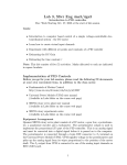
CanSat Ground Station
Electronics & IT
P5 Student Project
Autumn Semester 2010
Group 10gr503
Department of Electronic Systems
Aalborg University
Department of Electronic Systems
Electronics & IT
Fredrik Bajers Vej 7 B
9220 Aalborg Ø
Phone 9940 8600
http://es.aau.dk
Title: CanSat Ground Station
Subject: Distributed embedded systems in
cooperation with physical systems.
Project period:
P5, autumn semester 2010
Project group:
10gr503
Participants:
Kent Basselbjerg
Thomas L. Hansen
Peter B. Jørgensen
Niels G. Myrtue
Rasmus Pedersen
Bo Ø. Povey
Supervisor:
Jens Dalsgaard Nielsen
Number of copies: 8
Number of pages: 176 (last page is p. 168)
Attachments: 1 cd
Appendices: 7
Ended the 20/12 2010
Abstract:
Background
CanSat competetitions are held anually by several space
organizations. This project regards the development of
a ground station, that can support students participating in these competitions. The ground station must be
able to track the CanSats and communicate with them
wirelessly. Other projects have had the goal of designing
and constructing such CanSats. The WARP radio protocol has been developed in coorperation between these
projects, it allows the constructed ground station and
CanSats to work togther.
Results
The system consists of a ground station and a remote
user client. The ground station can communicate wirelessly with CanSat’s. The remote user client and ground
station can communicate through an Ethernet link, eg.
over the internet.
The ground station is designed as an embedded system
and connected to a pan & tilt platform with two PWMpowered DC-motors, and an Yagi-Uda type antenna attached. As the platform for the ground station software,
a preemptive real-time operating system is designed and
implemented on an ARM-based microcontoller.
The pan & tilt platform is modeled as two independent
second order systems. Non-linear corrections are introduced, in order to compensate for the non-linear nature
of the friction and gravity, affecting the platform. Feedback control is designed using frequency domain design
methods.
The user interface to the system is the remote user client,
developed as a Java based GUI application. This program allows the user to remotely control the ground station, and send commands to the CanSat. It also handles and saves incoming CanSat telemetry, relayed by
the ground station.
Conclusion
The final system is able to accommodate most of the
requirements. The antenna controller system has been
shown to be able to follow a simulated launch of a
CanSat. With further development, it is possible to make
the ground station system feasable for use in CanSat
competitions.
The contents of this report is freely available, but publication (with source reference) is only permitted as agreed with the authors.
Preface
This report has been composed by group 503 at the faculty of engineering-, nature- and
medical science at Aalborg University, in the period from 2-9-2010 to 20-12-2010. It is a 5.
semester project at the Department of Electronic Systems - Electronics and IT, and has
been created in cooperation with supervisor Jens Dalsgaard Nielsen. The general theme
of the project is distributed embedded systems in cooperation with physical systems.
In the project an antenna system for tracking a CanSat has been designed. The target
group for this report is university students and teachers.
Because the project is made mainly for educational purposes, the final product is not
to be thought of as having commercial value.
The report is divided into three main parts: “Project Specifications”, “Design &
Implementation” and “Assessment & Conclusion”. Referenced sources are denoted by a
number in square brackets, like: [1]. This number refers to the list of references, which
can be found on page 127. If the report is read electronically it is possible to jump to
chapters, sections, figures, tables and citations by “clicking” on their references. Different
acronyms and terms are widely used throughout the report. In appendix A on page 130
a list of these can be seen. The reader is advised to read this carefully. In the report
functions() and variables written in code, are emphasized by a different font.
Appendices are placed in the end of the report. These appendices contains test
journals, protocols and other things that support the development of the product as well
as the report. The appendices are denoted A, B, C and so on, while the test journals are
numbered. In appendix G on page 146 a schematic of the entire system and a part list
can be found. Along with the report a CD is enclosed, containing datasheets, developed
software, test software, Matlab scripts and a PDF version of this report. On the CD, a
folder with videos and pictures of the developed system can be found 1 . Throughout
the report, there will be referenced to material on the CD in this way, the full path can
be found as a footnote.
Kent Basselbjerg
Thomas L. Hansen
Peter B. Jørgensen
Niels G. Myrtue
Rasmus Pedersen
Bo Ø. Povey
1 /multimedia
v
Contents
1 Introduction
Part I
1
Project Specification
2 Preliminary Analysis
2.1 CanSat Competition . . . . . . . . . . . . . . . . . . . . . . . . . . . . . .
2.2 System Overview . . . . . . . . . . . . . . . . . . . . . . . . . . . . . . . .
2.3 WARP AAU Radio Protocol . . . . . . . . . . . . . . . . . . . . . . . . .
5
5
6
9
3 Requirements Specification
13
3.1 Use Cases . . . . . . . . . . . . . . . . . . . . . . . . . . . . . . . . . . . . 13
3.2 Requirements Specification . . . . . . . . . . . . . . . . . . . . . . . . . . 17
3.3 Acceptance Test Specification . . . . . . . . . . . . . . . . . . . . . . . . . 19
Part II Design & Implementation
4 Modularization
23
4.1 Utilized Hardware . . . . . . . . . . . . . . . . . . . . . . . . . . . . . . . 23
4.2 Remote User Client Protocol . . . . . . . . . . . . . . . . . . . . . . . . . 24
4.3 Ground Station Subtasks . . . . . . . . . . . . . . . . . . . . . . . . . . . 27
5 Real Time Operating System
5.1 System Calls . . . . . . . .
5.2 Multi-tasking . . . . . . . .
5.3 Fixed Priority Scheduling .
5.4 Verification . . . . . . . . .
.
.
.
.
.
.
.
.
.
.
.
.
.
.
.
.
.
.
.
.
.
.
.
.
.
.
.
.
.
.
.
.
.
.
.
.
.
.
.
.
.
.
.
.
.
.
.
.
.
.
.
.
.
.
.
.
31
31
33
35
36
6 Wired Communication with Remote User Client
6.1 Overview . . . . . . . . . . . . . . . . . . . . . . .
6.2 Ethernet Controller . . . . . . . . . . . . . . . . . .
6.3 Integrating the uIP TCP/IP Protocol Stack . . . .
6.4 Maximum Throughput and Verification . . . . . .
.
.
.
.
.
.
.
.
.
.
.
.
.
.
.
.
.
.
.
.
.
.
.
.
.
.
.
.
.
.
.
.
.
.
.
.
.
.
.
.
.
.
.
.
.
.
.
.
.
.
.
.
37
37
38
39
43
7 RF
7.1
7.2
7.3
7.4
.
.
.
.
.
.
.
.
.
.
.
.
.
.
.
.
.
.
.
.
.
.
.
.
.
.
.
.
.
.
.
.
.
.
.
.
.
.
.
.
.
.
.
.
.
.
.
.
.
.
.
.
45
45
46
47
49
.
.
.
.
.
.
.
.
.
.
.
.
Communication with CanSat
Basic Setup . . . . . . . . . . . .
Link Budget . . . . . . . . . . . .
Software for RF Communication
Verification . . . . . . . . . . . .
.
.
.
.
.
.
.
.
.
.
.
.
.
.
.
.
.
.
.
.
.
.
.
.
.
.
.
.
.
.
.
.
.
.
.
.
.
.
.
.
.
.
.
.
.
.
.
.
.
.
.
.
.
.
.
.
.
.
.
.
.
.
.
.
.
.
.
.
.
.
.
.
.
.
.
.
8 Modelling of Pan & Tilt Platform
51
8.1 Model Overview . . . . . . . . . . . . . . . . . . . . . . . . . . . . . . . . 51
8.2 Combining the Model . . . . . . . . . . . . . . . . . . . . . . . . . . . . . 55
vi
8.3
8.4
8.5
8.6
Friction . . . . . . . . . . . . . . . .
Non-linearity in Elevation Model . .
Parameter Determination and Model
Final Expression . . . . . . . . . . .
. . . . . . .
. . . . . . .
Verification
. . . . . . .
.
.
.
.
.
.
.
.
.
.
.
.
.
.
.
.
.
.
.
.
.
.
.
.
.
.
.
.
.
.
.
.
.
.
.
.
.
.
.
.
.
.
.
.
.
.
.
.
.
.
.
.
.
.
.
.
56
57
58
63
9 Feedback Control of Pan & Tilt Platform
9.1 Interpretation of the Requirement . . . .
9.2 Controller Design . . . . . . . . . . . . . .
9.3 Implementation . . . . . . . . . . . . . . .
9.4 Verification of Controllers . . . . . . . . .
.
.
.
.
.
.
.
.
.
.
.
.
.
.
.
.
.
.
.
.
.
.
.
.
.
.
.
.
.
.
.
.
.
.
.
.
.
.
.
.
.
.
.
.
.
.
.
.
.
.
.
.
.
.
.
.
.
.
.
.
.
.
.
.
.
.
.
.
.
.
.
.
65
65
66
75
86
10 Remote User Client
10.1 Overview and design . . . . . . .
10.2 User Interface and Functionalities
10.3 Threads . . . . . . . . . . . . . .
10.4 Receive and Send Methods . . .
10.5 Verification . . . . . . . . . . . .
10.6 Further Development . . . . . . .
.
.
.
.
.
.
.
.
.
.
.
.
.
.
.
.
.
.
.
.
.
.
.
.
.
.
.
.
.
.
.
.
.
.
.
.
.
.
.
.
.
.
.
.
.
.
.
.
.
.
.
.
.
.
.
.
.
.
.
.
.
.
.
.
.
.
.
.
.
.
.
.
.
.
.
.
.
.
.
.
.
.
.
.
.
.
.
.
.
.
.
.
.
.
.
.
.
.
.
.
.
.
.
.
.
.
.
.
91
91
93
100
101
103
103
.
.
.
.
.
.
.
.
.
.
.
.
.
.
.
.
.
.
.
.
.
.
.
.
.
.
.
.
.
.
11 Scheduling of Ground Station Software
105
11.1 Software modules . . . . . . . . . . . . . . . . . . . . . . . . . . . . . . . . 105
11.2 Scheduling . . . . . . . . . . . . . . . . . . . . . . . . . . . . . . . . . . . . 106
Part III Assessment & Conclusion
12 Acceptance Test
117
12.1 Tests . . . . . . . . . . . . . . . . . . . . . . . . . . . . . . . . . . . . . . . 117
13 Conclusion
121
14 Perspectives
123
14.1 Improvements . . . . . . . . . . . . . . . . . . . . . . . . . . . . . . . . . . 123
14.2 Usage in CanSat Competitions . . . . . . . . . . . . . . . . . . . . . . . . 124
References
125
Appendices
A
Word List . . . . . . . . . . . . . . . . . . . . .
B
WARP Protocol Specification . . . . . . . . . .
C
RUC Protocol Specification . . . . . . . . . . .
D
uIP Example Mainloop with ARP . . . . . . .
E
ARTOS Function Prototypes . . . . . . . . . .
F
CanSat Test Stand-in . . . . . . . . . . . . . .
G
Schematic, Part-list and Physical Construction
.
.
.
.
.
.
.
.
.
.
.
.
.
.
.
.
.
.
.
.
.
.
.
.
.
.
.
.
.
.
.
.
.
.
.
.
.
.
.
.
.
.
.
.
.
.
.
.
.
.
.
.
.
.
.
.
.
.
.
.
.
.
.
.
.
.
.
.
.
.
.
.
.
.
.
.
.
.
.
.
.
.
.
.
.
.
.
.
.
.
.
.
.
.
.
.
.
.
.
.
.
.
.
.
.
128
130
131
135
137
139
145
146
Test & Measurement Journals
1
Range Test of RF Communication . .
2
Test of RUC CSV File Saving . . . . .
3
Model Parameter Determination . . .
4
Controller Verification . . . . . . . . .
5
Measurement of Worst Case Execution
6
Acceptance Test 1 . . . . . . . . . . .
7
Acceptance Test 2 . . . . . . . . . . .
.
.
.
.
.
.
.
.
.
.
.
.
.
.
.
.
.
.
.
.
.
.
.
.
.
.
.
.
.
.
.
.
.
.
.
.
.
.
.
.
.
.
.
.
.
.
.
.
.
.
.
.
.
.
.
.
.
.
.
.
.
.
.
.
.
.
.
.
.
.
.
.
.
.
.
.
.
.
.
.
.
.
.
.
.
.
.
.
.
.
.
.
.
.
.
.
.
.
.
.
.
.
.
.
.
148
150
153
155
160
163
166
167
. . . .
. . . .
. . . .
. . . .
Times
. . . .
. . . .
.
.
.
.
.
.
.
vii
CHAPTER
Introduction
In August 2010 four students from Nørresundby Gymnasium participated in the European CanSat competition in Norway along with 10 other groups of students from upper
secondary schools. The competition was hosted by the European Space Agency (ESA)
in order to motivate young people to study science and technology[2], by having them
build and launch a CanSat. A CanSat is a tiny satellite, built to fit inside a standard
330 mL soda can. It is deployed from a rocket in an altitude of approximately 1 km
before parachuting back to Earth. During the travel the CanSat sends telemetry data to
a ground station to be used for educational purpose e.g. to calculate the apex (highest
point) of the flight.
The goal of the CanSat competitions is not to build real satellites, but rather to
have students gain insight into the process of building a real satellite. Many space
organisations have held CanSat competitions for students from upper secondary school
or universities[3],[4],[5]. These competitions seek to inspire young scholars to follow
careers within science and engineering. This way, the space organisations hope to ensure
the future workforce of scientists and engineers for developing space programmes.
The Danish Agency for Science, Technology and Innovation are considering hosting
a CanSat competition for students in danish upper secondary schools. Therefore, they
have requested Aalborg University to develop a CanSat kit. The kit must be designed
to be easy to use, low-cost, open source and based on off-the-shelf components. The kit
will consist of:
• An onboard CanSat controller.
• A radio communication link on a license free band.
• A sensor sub platform (possibility to extend with custom sensors).
• A ground station for communication with CanSat during flight.
In the fall semester 2010, at the time of writing, four groups of students at the department
of Electronic Systems at Aalborg University, are doing semester projects regarding the
development of this kit. Three groups put their focus on the CanSat itself and one
group focus on the ground station. The groups have cooperating, shared experiences,
and a common radio communication protocol has been developed in order to ensure
compatibility between CanSats and ground stations.
This report is the documentation of the work done by group 10gr503. The starting
point of this particular project is the development of the ground station with an automatic
1
1
Chapter 1. Introduction
satellite tracking antenna. Acquisition and saving of the CanSat telemetry data is a
crucial part of the CanSat project. Since the rocket propelled launch is a one time
opportunity, the main mission of the ground station is to gather and save as much
information about the flight as possible. To accomplish this task, precise tracking of the
CanSat is necessary in order to minimize the amount of lost information.
2
Part I
Project Specification
CHAPTER
Preliminary Analysis
The purpose of this chapter is to clarify the background and requirements for this project.
First the CanSat competition will be described in order to get an overview of what the
ground station system is going to be used for. Then a system overview identifies the
different components a ground station system consists of, and the technical aspects in designing and realising these units are discussed. A discussion of the design of the common
radio protocol between ground stations and CanSats follows. The final outcome of the
chapter is the foundation of the requirements specification.
2.1. CanSat Competition
The CanSat concept was introduced in the late 1990s by the American professor Robert
Twiggs[6]. Since then, several CanSat competitions have been held in the USA, Japan
and Europe with slightly different rules and requirements.
The CanSat competition, this project evolves around, is held by the European Space
Agency, ESA. The competition is aimed at students in the upper secondary school.
It was first held in 2010, where students from 11 different countries participated. In
august 2010 the students launched their CanSats from the Andøya Rocket Range, an
independent branch of the Norwegian Space Center.
Information about the CanSat competition in 2011 has not yet been published. Therefore this project is based on information for the 2010 competition [5]. Participating teams
must consist of 3-10 high-school students. They must build CanSats that measure air
temperature and air pressure. These data must then be transmitted to the ground station
at least once every second after release and during descend. In addition to this primary
mission, a secondary mission of free choice must be accomplished. The secondary mission
can be anything, as long as it has some technological, investigative or innovative value.
It could for example be:
• Advanced Telemetry: measurement of acceleration, GPS location or radiation levels.
• Telecommand: having the ground station send commands to the CanSat.
• Comeback: have the CanSat autonomously navigate to a target land point.
• Landing System: a safe landing system, such as a bespoke parachute or airbag.
5
2
Chapter 2. Preliminary Analysis
• Planetary Probe: Simulate an exploration flight to a new planet, e.g. taking measurements on the ground after landing.
The rules for the competition are not directly targeted at the ground station, they specify
requirements such as size and weight of the CanSat itself. The specific rules will thus
not be mentioned here, but they can be found on the ESA website [5].
2.2. System Overview
The purpose of this project, is to design and build a ground station for CanSat satellites.
This ground station must be able to receive data from and send data to the CanSats
constructed by other groups.
2.2.1
Project Contents
In previous years, a directional antenna has been used to receive the radio signals from
the CanSats. This is due to the fact, that the CanSats can only transmit a very weak
radio signal, because they can only contain small antennas. Also, they run on small
batteries and maximum transmission power is specified by government regulations. These
government regulations are investigated further in section 7 on page 45. This directional
antenna must thus be pointed in the direction of the CanSat at all times during flight. It
has been chosen, that this ground station system must have the following functionalities:
• Ability to automatically point the antenna at the CanSat and track it as it moves.
• Ability to receive the wireless data from the CanSat, namely telemetry data measured from onboard sensors, and transmit them in realtime to a computer located
elsewhere. This transmission is done via an internet connection. The receiving
computer is henceforth referred to as the “remote user client”, or just RUC.
• Facilitate control of the ground station from the remote user client.
An overview of the project content can be seen on figure 2.1.
Figure 2.1: This figure illustrates the CanSat, Ground Station and Remote User Client. The project
is limited to the objects contained within the boxes.
Note that the construction and design of the CanSat and the network between the ground
station and the remote user client, is not part of this project. The premise for choosing
6
Section 2.2. System Overview
the elements that the project contains, has primarily been that, they should contain
technical aspects, that the group would like to learn about:
• The automatic pointing of the antenna, requires the development of feedback control of the physical system consisting of the tilt and pan platform and antenna.
• The radio link to the CanSat, requires a data transfer protocol to be developed and
implemented.
• By having the ground station and remote user client placed at different locations,
a network connection must be established between them. Again, an application
level network communication protocol is needed for this link.
• The ground station is going to be an embedded system with real time and multitasking requirements. A real time operating system is thus required.
• The application on the remote user client must be a GUI application, that can
manage the GUI and service the network connection. To do this in a satisfactory
way, multi programming techniques must be used.
2.2.2
Technical Aspects
The ground station is implemented as an embedded system, that takes care of receiving
radio data from the CanSat, forwarding these to the remote user client and controlling
the antenna direction. The remote user client needs to be capable of saving the received
data and representing this to the user. Since a PC offers great conditions for data storage
and representation, the remote user client is implemented as a GUI application running
on such a system. The project thus consists of the following technical aspects, that are
implemented in the product:
• Automatic Antenna Direction Control
The antenna needs to be adjusted to point straight towards the CanSat at all times.
To ensure this functionality, a pan and tilt platform, assisted by a controller, is
utilized. The controller is designed and constructed by the project group, whereas
a pre built pan and tilt platform will be used. In order to design the controller, it
is necessary to design a mathematical model of how the motors on the pan and tilt
platform affect the direction the antenna is pointing.
In order to know which way to point the antenna, the ground station needs to
know where the CanSat is. For this, it has been chosen to require the CanSat to
be equipped with a GPS. These GPS coordinates will then be sent to the ground
station over the radio link, which can then be used to calculate in which direction
to point the antenna. CanSats that should be tracked automatically by the ground
station, must thus be equipped with a GPS. For this to work, the ground station
must know the GPS coordinates of its own location as well. Furthermore, it is
desirable to be able to override this automatic antenna control and manually control
the antenna. This can be used if the ground station is used with a CanSat that
do not contain a GPS or if the ground station looses track of the CanSat and thus
does not receive new GPS coordiantes anymore. The design and implementation
of the antenna control is described in chapter 9 on page 65.
• Radio Communication
The radio link from the CanSat to the ground station must be working on some
license free frequency band, because it is undesirable to require the schools using
the CanSat kit to acquire a license for the radio link. Pre built radio transceivers
are used for the transmission. Since the project group would like to work with
data protocols, it has been chosen that these radio transceivers should provide
7
Chapter 2. Preliminary Analysis
nothing but a (possibly unreliable) byte- or bit stream transmission. The design,
construction and implementation of the radio communication system is described
in chapter 7 on page 45.
• Network Based Connection
As illustrated on figure 2.1 on page 6, a network is used to connect the remote
user client to the ground station. It has been chosen to use the TCP/IP network
protocol suite on top of an Ethernet network. This way the network can be an
Ethernet cable, an existing LAN network or the internet. This gives the user great
flexibility in choosing how to connect the ground station and the remote user client.
The actual implementation of these protocols is described in chapter 6 on page 37.
• Remote User Client
The users that are going to utilize the CanSat kit and thus also the ground station and remote user client developed in this project, will be students from upper
secondary schools. It is thus vital that the system can be used by non-technical
people who haven’t worked with electronics before. Therefore, the remote user
client is developed as a GUI application on a PC. This GUI must be fairly intuitive
and easy to use. It has been chosen to use Java as the programming environment
for this application, since it provides an excellent cross-platform environment for
developing GUI applications. Java also provides great network support and it’s
easy to create multi-threaded applications, since this is supported at the language
level by Java. It should be noted however, that since the project group is receiving
courses on Java this semester, it is the obvious choice. The design and development
of the remote user client is described in chapter 10 on page 91.
• Realtime operating system
The ground station must be able to handle the connection to the CanSat, handle
the connection to the remote user client and perform the antenna pointing direction
control. This must all be done in parallel and in a timely manner. It has been chosen
to implement this on an embedded computer system running a real time operating
system. The design and implementation of this real time operating system is a
part of the project, because it presents some interesting technical challenges. It is
further described in chapter 5 on page 31.
• Telemetry Data Backup
One of the primary tasks of the ground station is to receive telemetry data from
the CanSat. Under normal operation the received CanSat data will be transferred
to the remote user client and saved as a file upon arrival there. The network link
may break however, and other unforeseen events e.g. a computer crash, could lead
to loss of incoming data. Therefore it is desired to save telemetry data to persistent
memory on the ground station as well. This is referred to as the telemetry data
backup. In case of link breakage or crash the data on the ground station would be
available for later retrieval. It is worth considering keeping a similar backup aboard
the CanSat, which could then be read after retrieving the CanSat after a flight, if
the radio link is unreliable or completely lost during the flight. The construction of
the CanSat is not part of this project though. Due to time constrains, the telemetry
data backup has not been implemented in the system.
• Event Log
It is desirable for the user to be able to analyze what happened during flight.
Therefore, the remote user client maintains a log of recorded system and user activity. This includes user interaction with the GUI and information about received
packets. This is called the event log. Implementation of this is described in the
chapter descibing the RUC, chapter 10 on page 91.
8
Section 2.3. WARP AAU Radio Protocol
2.3. WARP AAU Radio Protocol
In order to make it possible to use the ground station constructed in this project, with
the CanSats being designed by other project groups, a common protocol for the transfer
of data over the wireless link is to be defined. In this section, protocol requirements
originating from this project are analysed. Then the protocol design choices are discussed.
The protocol specification has been developed in cooperation with the remaining
groups working on CanSat kits at AAU in the autumn semester 2010. The final protocol
specification can be found in appendix B. It precisely outlines the technical aspects of the
protocol. Anyone should be able to implement the protocol by reading this specification,
but will not necessarily understand why the protocol is designed the way it is. It has
been chosen to name this protocol WARP, which is a recursive acronym for “WARP
AAU Radio Protocol”.
2.3.1
Protocol Requirements Set by This Project
Since the ground station needs GPS data from the CanSat in order to track it, it must
be able point the antenna towards the CanSat at all times, including during the launch
phase. This also enables collection of telemetry data during launch. The satellite will
be accelerated to it’s maximum speed very quickly, which requires the antenna control
to be very responsive. As the position changes rapidly, the ground station has to receive the position frequently. Should the ground station completely loose track of the
CanSat during launch, further tracking will be impossible as no updated GPS data will
be received.
These circumstances set a requirement to how old the latest received position of
the CanSat is allowed to be. This requirement is incorporated into the common radio
protocol. The following calculations gives an estimation of the minimum sample rate and
maximum latency of the CanSat GPS data, which are required for the ground station to
be able to track the CanSat during launch. First the maximum angular velocity of the
elevation angle is found. The timing requirements are then derived from this value.
Maximum angular velocity of tracking antenna
The purpose of the following calculations is to find the maximum angular velocity of the
elevation, which is required for the ground station antenna to track the CanSat.
The ground station is placed in a horizontal distance r from the launch site and the
altitude of the rocket is denoted h as shown in figure 2.2 on the next page. To calculate
the maximum angular velocity ωmax of the elevation of the ground station antenna, the
following scenario is assumed:
• The angular velocity of the elevation reaches it’s maximum value during the launch
phase (until rocket releases its payload).
• The rocket only moves along the vertical axis. This scenario is assumed because
the angular velocity required to track lateral movements of the rocket is expected
to be much smaller.
• The distance r = 400 m.
m
• The maximum velocity of the rocket vmax = 600 km
t = 166.7 s is reached with
m
m
a constant acceleration a = 20 · g = 20 · 9.82 s2 = 196.4 s2 and the velocity is
maintained during the rest of the launch phase. vmax is the highest expected
rocket velocity. In comparison the maximum velocity for the rocket used in the
ESA 2010 CanSat competition was 544 km
t [6]. The value of a comes from the
maximum acceleration a CanSat should be able to withstand [5].
9
Chapter 2. Preliminary Analysis
• The inaccuracy of the GPS data can be neglected, because it is small compared to
the horizontal distance r to the rocket.
Figure 2.2: Illustration of CanSat tracking during launch.
From these assumptions the movement of the rocket can be divided into the two phases,
constant acceleration and constant velocity. The angle between the ground plane and
a straight line from the ground station to the rocket is the desired elevation angle θ =
arctan( hr ). The altitude of the rocket h during the acceleration phase can be written as
h = 21 · a · t2 , where t is the time from the beginning of the launch. The angular velocity
of the elevation angle is the derivative of θ with respect to time. The angular velocity
during the acceleration phase ω1 is given by:
1
d arctan( 2
dθ
ω1 (t) =
=
dt
dt
art
= 2 1 2 4
r + 4a t
·a·t2
r )
(2.1)
(2.2)
A similar expression is found for the constant velocity phase:
ω2 (t) =
=
(t−t1 )
d arctan( h1 +vmax
)
r
dt
vmax
r+
where:
ω1
ω2
a
vmax
r
h1
t1
t
(h1 +vmax (t−t1 ))2
r
is the angular velocity of the elevation during the constant acceleration
phase
is the angular velocity of the elevation during the constant velocity
phase
is the acceleration during the constant acceleration phase
is the maximum velocity of the rocket
is the horizontal distance between the ground station and the launch
site
is the distance travelled by the rocket during the constant acceleration
phase
is the duration of the constant acceleration phase
is the time since the beginning of the launch
(2.3)
(2.4)
[s−1 ]
[s−1 ]
[ sm2 ]
[ ms ]
[m]
[m]
[s]
[s]
With the assumed values for r, a and vmax the angular velocity of the elevation angle
versus time can be plotted, as shown in figure 2.3 on the facing page. The angular velocity increases during the acceleration phase and the maximum velocity is reached in
under 1 second. From the graph the maximum angular velocity ωmax can be read as
approximately 0.4 rad/s. Note that because of the assumptions made in the calculations,
the angular velocity found is a rough estimation.
10
Section 2.3. WARP AAU Radio Protocol
0.5
ω [rad/s]
0.4
0.3
0.2
0.1
0
0
0.5
1
1.5
2
2.5
t [s]
3
3.5
4
4.5
5
Figure 2.3: Calculated angular velocity of the desired ground station elevation versus time during the
launch
GPS position update time
The maximum angular velocity of the antenna tracking platform has been calculated to
approximately 0.4 rad/s. This value can now be used to get an idea of how often the GPS
position must be updated in order to be able to track the CanSat with the antenna. It is
assumed that the ground station will be able to track the CanSat if the latest elevation
angle fed as reference position to the controller never deviates more than 10° from the
real value. At an angular velocity of 0.4 rad/s a rotation of 10° takes 436 ms. If the GPS
sample rate is set to 5 Hz, the sample period is 200 ms. This leaves 236 ms for the GPS
data to be transmitted and fed into the controller. It is assumed that from the time
the CanSat has completed transmitting a package with the GPS data, until the ground
station has passed it to the controller, no more than 36 ms will pass. Therefore, it is a
requirement to the CanSat, that no more than 200 ms may pass, from the time a GPS
sample is taken until the package with the data has been transmitted.
However it is clear from the above that packet loss in the CanSat to ground station
communication during the launch, can be fatal for the automatic antenna tracking system. Thus a panic action should be considered in case of a lost link. For example the
current CanSat position could be extrapolated based on previously obtained GPS data.
2.3.2
Protocol Design Decisions
Before designing the protocol, it is worth considering what the protocol’s job is, which
features it should contain and so forth. This can be used as the basis of how the protocol
should be designed. The protocol is to be used on top of a wireless radio data link. This
link is a byte stream, i.e. a channel, where bytes are put into one end and taken out of
the other. Since it’s a wireless link, no assurances are made that the bytes are transfered
undamaged. It is worth noting, that often the rockets will bring multiple (typically two)
CanSats into the air at the same time. Measures must thus be taken to ensure the radio
link will be working correctly, even if multiple CanSats, all using the WARP protocol,
are airborne at the same time. There might also be multiple ground stations, all using
WARP. It is desired however, that different CanSats - ground station pairs use different
frequency bands for their communication, so interference between them is avoided.
Package Delimiting
A way to delimit each chunk of information is needed. It has been chosen to use a package
oriented protocol. To delimit these packages, a start and a stop byte will be used. The
advantage of using this scheme compared to fx. having a length field in the packages, is
that it is known that if an (unescaped) start byte is received, then that is the start of
11
Chapter 2. Preliminary Analysis
the next package. This will thus correct any errors in the transmission. If only a length
field was used, errors in one of these length fields, would result in all following packages
not being received correctly, since the package limits would be unknown. This requires
all occurrences of the start and stop byte to be escaped, which will be done using byte
stuffing.
Implementing devices that adhere to the protocol, is much easier, if a maximum
package size has been specified. This way, it is known how much buffer space to allocate
for received packages. This maximum package size will be specified as the package size
before adding start- and stop bytes and escape characters, since it is expected that devices
will be removing these bytes before saving them into a buffer. The maximum package
size has been chosen to be 150 bytes.
Since errors may occur in the bytes transmitted over the wireless link, a way to ensure
that the package was transferred without any errors is required. For this, a checksum
field will be used.
Transfer of Telemetry Data
Obviously, it should be possible to transmit measured telemetry data from a CanSat to
the ground station. The measurement will likely happen at a fixed time rate, e.g. 2 Hz.
Each time such a measurement has been performed, it should be transmitted to the
ground station. If there is bandwidth and computation power left over, it is better spent
on increasing the rate at which measurements are taken and transmitted, than using them
on some acknowledgement scheme that ensures arrival of every measurement taken. For
this reason, an unacknowledged transmission scheme will be used for this type of data,
where a CanSat just transmits a number of packages and the ground station receives as
many of these as the circumstances allows it to.
Remote Control of CanSats
It has been chosen that the students should be offered the possibility to perform some
sort of remote control of a CanSat, while they are airborne. The communication protocol,
must thus be 2-way and allow commands to be sent from the ground station to a CanSat.
What these commands do, is not to be specified by the protocol. To keep the protocol
simple, it has been chosen that the command is sent as a “command number” that can
then be used to execute the corresponding function on the CanSat. It will not be possible
to send arguments along with the commands. It is required that only one ground station
is communicating with each CanSat.
A transmission scheme similar to the one used for transfer of telemetry data, cannot
be used for this. When the user has asked for a command to be executed, he needs to
be assured that this command has actually been performed. Therefore a scheme where a
CanSat has to send an acknowledgement after successfully receiving a command package
will be used.
It is desired to ensure that the ground station, doesn’t transmit a package, at the
same time as the CanSat is transmitting a package. For this, a flag in the packages going
from the CanSat to the ground station, is used to indicate if the ground station is allowed
to transmit in a time interval following the reception of the package. This time interval
has been chosen to be 50 ms. As it will be shown in chapter 11, sending a command
package in the used setup will take 8 ms.
12
CHAPTER
Requirements Specification
The analysis in the previous chapter outlines some of the aspects that form the basis of
this project. It described the basic composition of the project and the product to be designed. In the following chapter, use cases are used to describe the desired functionalities
of the final product, seen from the users perspective. Next, a requirement specification
outlines the technical requirements that the product should comply with. Based on this,
an acceptance test specification is made. If the product can pass this test, it complies
with the requirements specification. The use cases and the requirements specification are
based on the previous analysis.
3.1. Use Cases
To establish an overview of what the product should contain seen from the users perspective, a use case diagram has been drawn up. The diagram is based on the preliminary
analysis and the chosen areas of focus, described in chapter 2. Each use case describes
a functionality that needs to be incorporated into the final product. These use cases
set the scope for the product, but without eliminating the opportunity to add extra
functionality. The use case diagram can be seen in figure 3.1 on the next page.
3.1.1
Actors
The system has the following two actors:
• User
The user could be a student at an upper secondary school, who is participating in
the CanSat competition.
• CanSat
The CanSat is what needs to be tracked by the ground station. It provides the
ground station with different kinds of data, such as telemetry data like temperature
and pressure.
3.1.2
Description of Use Cases
The following lists the use cases and describes the goals, normalscenarios and in some
cases exceptions of the use cases. The goal description of each use case explains the
13
3
Chapter 3. Requirements Specification
Figure 3.1: This figure illustrates the products use case diagram.
desired result from the action performed. The normalscenario describes the dialogue
between user and system. The exceptions describes how the system should act if an
error occurs.
1: Connect to Ground Station
Goal description:
The user establishes a connection to the ground station.
Normal scenario:
1. User: Sends a connection request to the ground
station.
2. System: Receives the request and establishes a
connection.
3. System: Acknowledges that the connection has
been established.
Exceptions:
• No connection can be established
The user is informed that the connection could not
be established, and is given the opportunity to try
again.
2: Show Antenna Direction Info
14
Section 3.1. Use Cases
Goal description:
The current position of the antenna is shown to the user.
Normal scenario:
1. User: Queries the system for the current antenna
position.
2. System: Receives the query and shows the current
position.
Exceptions:
• Current position cannot be determined
No antenna direction is shown.
3: Show Sensor Data
Goal description:
Data from the user-specified sensors on board the
CanSat, is shown to the user.
Normal scenario:
1. User: Queries the system for CanSat sensor data.
2. System:
data.
Receives the query and shows sensor
4: Enable Manual Antenna Direction Control
Goal description:
The user can adjust the system’s antenna.
Normal scenario:
1. User: Changes the antenna position configuration.
2. System: Receives new configuration and adjusts
the antenna.
Exceptions:
• The user specifies an invalid configuration
The system ignores the new configuration, and
warns the user.
5: Enable Automatic Antenna Direction Control
Goal description:
The system will take control of adjusting the antenna
direction.
15
Chapter 3. Requirements Specification
Normal scenario:
1. User: Queries the system to enable automatic antenna direction control.
2. System: Receives the query and takes control of
the antenna.
Exceptions:
• The system is set to conformance class 1, or
no ground station location is set
The system ignores the user request.
6: Specify CanSat ID
Goal description:
The system will store and use the specified CanSat ID.
Normal scenario:
1. User: Specifies the desired ID.
2. System: Receives the ID and stores it.
Exceptions:
• The user specifies an invalid CanSat ID
The system ignores the user input, and warns the
user.
7: Save Sensor Data
Goal description:
The user specifies a destination for the saved data.
Normal scenario:
1. System: Queries the user to specify a file destination to store the data.
2. User: Specifies a destination.
Exceptions:
• The user specifies an invalid file destination
The system ignores the file destination, and the
user is given the opportunity to retry.
8: Retrieve Ground Station Telemetry Data Backup
Goal description:
16
The user can send a request specifying that he/she wants
to obtain the ground station telemetry data backup.
Section 3.2. Requirements Specification
Normal scenario:
1. User: Queries the system to retrieve telemetry
data backup from the ground station.
2. System: Receives the query and attempt to retrieve the backup.
Exceptions:
• The ground station telemetry data backup
is empty
The system reports that the requested backup is
empty.
9: Send Commands to CanSat
Goal description:
The user can send different commands from the system
to the CanSat.
Normal scenario:
1. User: Queries the system to send commands to
the CanSat.
2. System: Receives the query and sends the specified command to the CanSat.
Exceptions:
• The requested command never reaches the
CanSat
If the system doesn’t receive an acknowledgement from the CanSat, the command will timeout.
When the command times out, it will be re-sent.
This procedure will be repeated until the system receives the acknowledgement.
3.2. Requirements Specification
The purpose of this chapter is to define and specify the requirements for the product.
These requirements are based on the general goal of the project and the previous analysis
of the system. The final product must comply with the following requirements:
Requirement 1. Must implement and adhere to the WARP protocol.
To be able to receive and process data from any CanSat, the ground station must implement the WARP protocol described in appendix B.
Requirement 2. Must implement and adhere to TCP/IP and Ethernet protocols.
The ground station will be connected to a network via an 8P8C-connector (also known
as RJ45-connector). This network will be TCP/IP based and the connection to it will be
17
Chapter 3. Requirements Specification
an Ethernet connection. The ground station and RUC must thus adhere to the TCP/IP
protocol suite and the Ethernet protocol.
Requirement 3. No more than 200 ms may pass from a package is received on
the ground station’s wireless link, until the processed package containing this
information, is sent to the RUC, if this is connected through a direct Ethernet
cable. This requirement will ensure a certain response time for the user when using the
system, by limiting the ground station’s package processing time. It is assumed that the
response time of the RUC is insignificant, compared to the processing time of the ground
station. This assumption is based on the fact that the ground station is implemented on
an embedded system, and the RUC is implemented on a PC.
Requirement 4. The RUC must save all received data as a comma separated
values file (CSV).
This requirement stems from the need to save all recorded data in an easily handled
format. CSV is cleartext with a simple format and is supported by many applications.
Requirement 5. If the RUC crashes, any data that already has been received,
must not be lost.
In order to achieve this requirement, all data processed by the RUC should be saved to
a file immediately after reception.
Requirement 6. The ground station must keep a backup of the latest received
telemetry data. This backup must contain data from the last 5 minutes or
more, given a package rate of 5 Hz with each package being the maximum
package size (150 bytes).
If the connection to the RUC is lost prior to or during a flight, it is desirable to backup
all received data. It noted that the rules for the competition state that a CanSat cannot
be airborne for any more than 120 s [5]. It is estimated that a data recording won’t
last for any more than 5 minutes and the maximum package rate will not be more than
5 Hz. Please note the maximum package size includes some header fields, which can be
omitted.
Requirement 7. The connection between ground station and CanSat must
be able to transmit 60 byte packages at a distance of 1.5 km with a maximum
package loss of 10 %. This is assuming that the CanSat and ground station
are placed in line of sight, the CanSat is within the antennas half-power
beamwidth and the package transmission rate is 5 Hz.
The 60 byte packages are used, to test the wireless connection at an expected normal
work load. The distance of 1.5 km is the estimated distance between the ground station
and the CanSat after launch. Notice that some package types are acknowledged in the
WARP protocol, described in appendix B on page 131. As a result, the actual package
loss will be less than the results of this test. Please note that this requirement depends
on the CanSat, which is constructed by other groups.
Requirement 8. The ground station must be able to control the antenna so
that an object following the launch graph on figure 2.3 on page 11 can be
tracked. The target must be within the half-power beamwidth of the antenna
at all times.
This requirement will ensure that a CanSat can be tracked during launch. It is assumed
that the CanSat is easily tracked during its descend, if it can be tracked during the launch
phase. The target must always be within the half-power beamwidth of the antenna, to
ensure that the ground station and CanSat antennas can ’see’ each other at any given
moment. Notice the half-power beamwidth is determined by the utilized ground station
antenna.
18
Section 3.3. Acceptance Test Specification
3.3. Acceptance Test Specification
The purpose of this section is to describe which tests needs to be performed on the
designed system to ensure that it meets the system requirements. The requirements can
be seen in section 3.2 on page 17. These tests are as follows, to see more details about
how these tests are performed, see chapter 12 on page 117.
Test 1. Covers Requirement 1 and 2
Packages adhering the WARP protocol are sent to the ground station. On the RUC, an
Ethernet connection is established, and a specific package format from a specific CanSat
ID is to be expected. The packages send will be marked as originating from two different CanSat’s by setting different CanSat ID’s in the packages. These packages will be
transmitted for at least five minutes. The packages with the matching CanSat ID must
be transmitted at least five times per second.
In order to pass this test, the system must filter out the packages with the wrong CanSat
ID. It also has to retrieve the data from all the correctly received packages with the
matching ID, and display these on the RUC.
Test 2. Covers Requirement 3
A CanSat telemetry data package is sent to the ground station. Once this is received
a timer will be started. The ground station will then prepare a package containing the
received data for the RUC protocol and transmit it. The package payload will be 150
bytes. The ground station and RUC will be connected directly through an Ethernet cable.
Once the package has been transmitted, the timer will be stopped. This is repeated for
1000 packages, and the worst-case time is extracted.
If the worst-case time is less than 200 ms, this test is passed.
Test 3. Covers Requirement 4 and 5
10,000 packages with known data are sent to the RUC, using the RUC protocol. The saved
data is compared with the data received, to see if they were stored correctly. Afterwards,
the test is repeated, but this time, the RUC is terminated by the OS, halfway through
receiving the data.
In order to pass this test, all received packages must, in both cases, be stored correctly.
Test 4. Covers Requirement 6
The ground station is set to track a CanSat, with a specific CanSat ID. Packages adhering the WARP protocol with this specific ID, is send to the ground station, at a rate
of 5 Hz with each package being the maximum package size (150 bytes). The RUC is
then disconnected from the ground station. After 5 minutes, the package transmission is
stopped. The RUC is then reconnected to the ground station, and the stored data in the
ground station data back up is requested.
In order to pass this test, the ground station must be able to send the last 5 minutes of
CanSat telemetry received, to the RUC.
Test 5. Covers Requirement 7
A ground station and a CanSat is placed in line of sight, at a distance of 1.5 km. The
RUC is then connected to the ground station, and the corresponding SatID is specified.
The CanSat is fitted with a serial connection which writes the received data to a computer,
and enables it to send packages on demand. At a certain time, a stopwatch is started,
and the CanSat is set to transmit 60 byte packages, at a rate of 5 Hz. After 5 minutes,
the CanSat stops transmitting, and the received packages are inspected. Afterwards, this
is repeated in the opposite direction.
In order to pass this test, no more than 10% package loss is permitted, in either direction.
This is calculated from the expected number of packages, relative to the number of valid
packages received.
19
Chapter 3. Requirements Specification
Test 6. Covers Requirement 8
The ground station is set to move the antenna along a predetermined path, as described in
requirement 8. Using saved information from the controller, such as where the antenna is
moving towards, and where its currently located, the maximum deviation is determined.
To pass this test, the maximum deviation must remain within the half-power beamwidth
of the antenna, at any given time.
20
Part II
Design & Implementation
CHAPTER
Modularization
After having completed the initial analysis of the system and having specified requirements
for it, the design of the system can begin. In section 2.2.1 on page 6 an outline of the
system components is shown. It can be seen that, the ground station has to be connected
to the remote user client over a TCP/IP based network. In the following, the application
level protocol for the communication over this network, will be defined. This protocol
defines the interface between the two major subsystems: the ground station system and
the remote user client. The ground station functionality can furthermore naturally be
divided into a number of subtasks. This division into subtasks will be described, thus
further modularizing the system. For this decomposition of ground station tasks, the
Hard Real Time Hierarchic Object-Oriented Design method (HRT-HOOD) is used.
4.1. Utilized Hardware
Before going into further details with the breakdown of the systems into smaller parts,
an overview of the system is given. This overview is shown in figure 4.1 on the next page.
The figure emphasizes which hardware components are used in the system and how they
are connected.
As the base for developing the ground station, a development board based on the
ARM7TDMI [7] CPU core has been chosen. The Mini-Max/ARM-E development board
from BiPOM Electronics [8], has an on board Ethernet controller chip, which makes it
easier to develop the Ethernet support required for the ground station. The development
board is based on the LPC2138 microcontroller from NXP [9],[10]. A summary of the
NXP LPC2138 features:
• ARM7TDMI CPU core, that can be clocked at speeds up to 60 MHz.
• 32 KiB RAM
• 512 KiB flash ROM
• Usual microcontroller features: 6 x PWM, 2 x SPI, 2 x I2C, 2 x UART, ADC, DAC
and Timer/Counter, all with various interrupt possibilities.
• Debugging and programming over JTAG.
For wireless communication with the CanSat, the RFM12B [11], [12] transceiver is used,
more details can be found in chapter 7 on page 45.
23
4
Chapter 4. Modularization
Figure 4.1: Overview of the hardware used in the system
A full list of utilized hardware, a total schematic and the physical construction of the
system can be seen in appendix G on page 146.
4.2. Remote User Client Protocol
All user-interaction with the ground station is done through the remote user client.
The communication between the ground station and the RUC, is done over a TCP/IP
connection. On top of this TCP/IP connection, an application level protocol must be
defined, this protocol will be referred to as the RUC protocol.
4.2.1
Information to be handled
The information going from the RUC to the ground station primarily consists of commands and configuration of what the ground station should do. This includes:
• Ask the ground station to calibrate the antenna direction control, see section 9.3.5
on page 82 for more details.
• Specify whether to use automatic (based on GPS information received from the
CanSat) or manual control of antenna pointing direction.
• When using manual control, specify wanted azimuth and elevation of the antenna.
• Set GPS location of ground station, which is used to calculate the direction to point
the antenna, when using automatic antenna direction control.
• Set ID of the CanSat that should be tracked. This corresponds to the SatID in the
WARP protocol packets received from the CanSats.
24
Section 4.2. Remote User Client Protocol
• To illustrate the effect of different types of feedback control, it can be specified
which type of feedback control should be used. See section 9.3.5 on page 82 for
more details.
• Retrieve saved telemetry data from the telemetry data backup. Due to time constrains, this has not been implemented in the ground station, but it is included in
the protocol.
• Ask the ground station to send a command to the CanSat.
The ground station will also be sending information to the RUC, which will primarily
consist of data:
• Telemetry data received from CanSat. This must be displayed to the user and it
must be possible for the user to save this data in a CSV file.
• Information about the antenna position. Two value sets are to be sent: Current
(actually measured antenna position) and wanted position (position being fed into
the controller). This information must be shown to the user, who can then decide if
manual or automatic antenna control is to be used. By both supplying the wanted
and current antenna position, it is possible for the user to see if the feedback control
is able to follow the antenna position that is wanted. This information must be
sent at a high rate, so that it can be used to test the feedback control as well. The
RUC should save the received information about antenna position in a file, so that
it can be analyzed when testing the feedback control of the pan & tilt platform.
• Acknowledgment of commands previously sent to the CanSat.
4.2.2
Underlying Protocol
TCP has been chosen, because it provides reliable connection oriented byte-stream transfer between two hosts, and it is widely supported by existing networks and hardware.
This means that TCP guarantees that sent data will ultimately arrive in the order they
were sent and without errors. The most obvious alternative to TCP is the UDP protocol. It is fundamentally different from TCP, since it’s datagram oriented instead of
connection oriented. UDP doesn’t make any guarantees about data actually being delivered, data integrity on delivery or the order in which the data is delivered. The RUC
to ground station connection requires all the reliability provided by TCP, if for example
two commands to set the CanSat ID are sent quickly after each other, the order they
arrive at the ground station determines which one will ultimately be effective. If UDP
was used, basically all the reliability that TCP provides had to be reimplemented in the
RUC protocol, therefore TCP has been chosen.
4.2.3
Effect of Large Latencies
It must be considered how the system reacts to large latency times on the network.
The network connection may go through the Internet, which is a very likely source of
considerable latencies. These may for example be caused by large physical distances
between hosts, congestion in the network, large data loss rates (which results in many
retransmissions) and more. This will obviously only be the case when connecting to the
ground station remotely. The effect of large latencies on the different types of data on
the RUC to ground station connection is:
• Telemetry data from ground station to RUC.
Latency here will result in the user experiencing that the data shown to him/her,
is not the most current data. This is an acceptable effect, since the data will
25
Chapter 4. Modularization
ultimately arrive and the data most often will be saved for later analysis. It is
useful for the user to know at which time the telemetry data was received from
the CanSat (eg. to perform calculations of speed based on GPS position data).
This information is not included in the WARP package. Since the latency from
ground station to the RUC may vary, a timestamp specifying the arrival time of
the telemetry data cannot be done on the RUC. The ground station must thus
send a timestamp along with each package containing telemetry data, specifying
the time the data was received from the CanSat. The timestamp is only used to
calculate the relative time between packages, and has been chosen to be the time in
milliseconds since any arbitrary reference time (likely the time the ground station
was started).
• Antenna position information from ground station to RUC and specification of azimuth and elevation when using manual antenna control.
If the user is trying to control the antenna position over a high-latency network, the
latency will be very noticeable, since there will be a time delay from specifying a
wanted antenna position until the antenna starts moving towards the specified position. Furthermore, there will be a delay until the new antenna position is shown
in the RUC. This will give the user a feeling of unresponsiveness, but this issue
cannot be avoided.
As with the telemetry data, it is desirable to know at which relative times the
antenna position data was captured and a timestamp must be sent along in this
case as well.
• Configuration setting commands from RUC to ground station.
This includes specifying CanSat ID, setting ground station GPS location, asking
ground station to calibrate, specifying automatic/manual control, specifying feedback controller type and asking to receive telemetry data backup.
Obviously latency here, will result in a delay from the time the user specifies a
setting to the time it takes effect. This effect cannot be avoided. If the latency
is large, it is possible that multiple configuration setting commands specifying different values for a setting, will be “stored” in the network. Since TCP guarantees
correct reception order of the data, the last issued setting command will be the one
that is received last, and thus also the setting that will be effective, which is the
desired behaviour.
• CanSat commands from RUC to ground station and acknowledgment
thereof.
When sending commands to the CanSat, the WARP protocol specifies that the
CanSat must acknowledge successful reception of the command. This information
should be passed to the user. There might be a considerable delay from sending
a CanSat command until it has actually been delivered. The command has to be
transferred from the RUC to the ground station, then over the wireless link to
the CanSat, which then acknowledges the reception of the command. Hereafter
the ground station must forward the acknowledge to the RUC. The part that is
transferred over the wireless link may require some retransmissions if the link is
bad, which will further delay the delivery of the command.
If the user doesn’t receive an acknowledge that his command was send relatively
fast, he might think the try was unsuccessful and try again. However the command
or the acknowledge thereof may just be “stored” somewhere in the network and
the user ends up having sent a number of commands, even though he only wanted
to send one. Therefore it has been chosen, that once a CanSat command has been
sent, another one cannot be sent until the first one has been acknowledged. This
also simplifies the protocol, since the CanSat command acknowledge sent from the
26
Section 4.3. Ground Station Subtasks
ground station to the RUC, will always be an acknowledge of the last command
sent.
These considerations have been part of the base, from which the protocol has been
designed.
4.2.4
Protocol Outline
The RUC protocol uses one-way messages, ie. when sending a message there is no direct
reply message. As described above, this is acceptable, also with large network latencies.
TCP provides a byte-stream, ie. it does not preserve package boundaries, so the RUC
protocol must provide a way to distinguish messages from each other in the byte stream.
For this, each message is put into a package, and each package is started by a start byte
and then followed by a length field, specifying the length of the package. Occurrences
of the start byte in the package are escaped using byte stuffing. No checksum is used,
since TCP guarantees data integrity. The details of the RUC protocol can be found in
appendix C on page 135.
4.3. Ground Station Subtasks
To support the design of the ground station, Hard Real Time Hierarchical Object Oriented Design (HRT-HOOD) is used. The method is used as described by Burns and
Wellings [13]. HRT-HOOD is a structured software design method for hard real time
systems. The ground station contains both software and hardware parts, but the design
of the ground station is done, by considering it solely as a software system. This is done
because the interface between the different parts of the system lie in software.
HRT-HOOD is hierarchical and uses a top-down approach. It is object oriented, not in
the C++/Java understanding of object orientation, but in the way that all tasks/modules
are described as objects that provide interfaces for other objects to use. The objects
express pieces of code to execute and not data structures (HRT-HOOD doesn’t concern
itself with the data structures of the software system at all). The design method is
based on decomposing the complete system into a number of objects. These objects
can then again be analyzed and decomposed into smaller objects. This hierarchical
decomposition continue until a sufficient amount of subdivision is achieved. The concept
of breaking down a system into smaller, more manageable, subsystems, is a common
base for almost all system design methods. What is special about HRT-HOOD and the
reason for choosing it, is that it provides a framework for graphically representing the
objects and their relations.
4.3.1
Usage in This Project
The design life cycle of HRT-HOOD is shown in figure 4.2 on the next page. It starts
out with the requirements specification, after which the logical architecture design is
done. It is here, the decomposition into objects is done. The physical architecture
design maps the designed system onto the platform (hardware and kernel) available.
Schedulability analysis is performed to analyze if the platform is sufficiently powerful for
the job. Detailed design and coding follows, implementing the software. At last HRTHOOD specifies that testing should be done. As with all software design methods, a
perfect design cannot be made the first time, so some iteration between the design stages
is to be expected, as shown by the arrows to the left in figure 4.2 on the following page.
In this project, the HRT-HOOD design life cycle is not used as described above.
The decomposition is started below to specify which subobjects should be constructed
and the interface between them. Only a first level decomposition is performed here.
27
Chapter 4. Modularization
Figure 4.2: Life cycle of the HRT-HOOD design method. [13]
When designing and implementing the individual subobjects, the objects are further
decomposed. After this, no physical architecture design is performed, instead detailed
design and coding of the subobjects is done. Hereafter measurements of the execution
time of the code, is used to perform an schedulability analysis, to ensure the system will
satisfy the timing requirements set to it. Before constructing the subobjects, an operating
system that implements the required multiprogramming facilities must be employed.
4.3.2
HRT-HOOD Objects
An object in HRT-HOOD is represented graphically as shown in figure 4.3 on the next
page. Each object specifies it’s name, type and the operations that they provide. The
operations of an object make up the interface it provides to other objects. 5 types of
objects exists, each describing when the code of the object is executed. These are as
follows:
A - Active The most general type of object, it has no restrictions placed on them. May
control when invocations of their operations are executed. Can be decomposed into
a number of the remaining object types.
P - Passive When invoking an operation on a passive object, it is performed immediately. This effectively corresponds to a call to a method in fx. C, which is also the
way these object types are implemented.
Pr - Protected Represents code or data that must be accessed under mutual exclusion.
C - Cyclic Periodic activities that execute irrespectively of whether there are any of
it’s operations that have been invoked.
S - Sporadic Objects that start executing at arbitrary time instances. These are often
started by an interrupt. They have a minimum arrival time associated with them,
specifying the maximum rate at which they occur.
Having mentioned the different object types, the relations between objects can be explained. There are many different types of “execution requests” in HRT-HOOD, each
describing a way one object can invoke an operation of another object. Here, only these
will be mentioned and used:
28
Section 4.3. Ground Station Subtasks
Figure 4.3: Graphical way of representing a HRT-HOOD object. [13]
ASER - Asynchronous Execution Request When an operation is invoked by an
ASER, the caller is not blocked, but continues to execute. The execution request
is noted and performed by the called object at some later time.
ASER BY IT - Asynchronous Execution Request from Interrupt Same as ASER,
but is invoked by an interrupt, either via a synchronizing semaphore or directly as
an interrupt handler.
HSER - Highly Synchronous Execution Request The calling object is blocked until the requested operation has been completed. Effectively a regular call to a
method in C.
PSER - Protected Synchronous Execution Request The same as HSER but invoked on a protected object, which means the calling task will be additionally
blocked if another object is using the object.
) labeled with a brief deData flow between objects is represented by an arrow (
scription of the data. There exists rules concerning which object types can include which
objects and which relations can exist between each object type, for more info, see [13].
4.3.3
Decomposition of Ground Station Software into Objects
The ground station system basically has three natural objects:
• Control the position of the antenna, based on either GPS data from the CanSat or
a manual specification of the position from the user.
• Handle the data received from the CanSat and send commands to it, based on the
specifications in the WARP protocol.
• Handle the TCP/IP/Ethernet connection to the RUC, which basically means implementing a stack of handlers for the protocol layers used by the link:
◦ Interface to the ENC28j60 Ethernet controller and handle Ethernet level packages.
◦ Handle the TCP- & IP protocol layers.
◦ Receive and send packages in compliance with the RUC protocol.
These 3 objects are shown in figure 4.3. They are all active objects, that thus can be
broken down into a number of smaller objects. It can be seen that, sending a package on
the RF CanSat link or to the RUC through Ethernet, is done as asynchronous execution
requests, ie. the transmission of the package is queued and then performed whenever the
link is ready for the transmission. Upon reception of a package in one of the two links,
the package is decoded and the required action is performed immediately by performing
synchronous calls to the antenna controller or ASER’s to send package on the other link.
For example, reception of telemetry data from the CanSat would result in an ASER to
the Ethernet & RUC protocol object, asking it to forward the received data to the RUC.
29
Chapter 4. Modularization
Figure 4.4: RT-HOOD Logical Architecture Design of the Ground Station
Summary
Above, the basic platform for constructing the ground station system has been chosen.
Also, the overall structure of the software to be executed on the ground station has been
designed. This allows for each ground station subsystem to be designed in detail and
implemented independently. The interface between the RUC and ground station is the
application level protocol used on the TCP/IP connection between them. This protocol
has been specified as well, which allows for the RUC and ground station to be developed
in parallel.
30
CHAPTER
Real Time Operating System
To implement the system described in chapter 4, a real-time multi-tasking operating system is required. Real-time means the ability to fulfill strict timing demands e.g. reacting
to incoming events before a certain deadline. A multi-tasking environment introduces concurrent execution of different tasks from the programmer’s point of view, which supports
the HRT-HOOD design paradigm well. This chapter regards the design and implementation of the operating system tailored for this project. Overall the system must have the
following features:
• Concurrent (pseudo parallel) execution of several prioritized tasks.
• Synchronization and message passing between tasks.
• Scheduling and execution of periodic tasks.
The operating system in this project is dubbed ARTOS, which is an acronym of ARM
Real-Time Operating System. Throughout this chapter the design and inner workings
of ARTOS will be discussed. The chapter ends with a verification test of the operating
system’s functionality.
5.1. System Calls
System calls (or syscalls) represents the interface between user programs and the operating system. In ARTOS there are 14 different system calls, which are shown in table 5.1
on the next page. These are supposed to give an overview of the different features of the
OS. The prototypes for these functions are located in “os.h” in the ground station source
code found on the CD 1 . See appendix E on page 139 for more details of the prototypes
and their arguments. The implementation of the OS is found in “os.c” and some low-level
routines are written in assembly and can be found in “os.S”. Reference documentation
for the ground station software is generated with the Doxygen documentation tool, and
can be found on the CD 2 .
In order to describe how system calls are processed, we need to look into the different
execution or processor modes of the hardware platform. The ARM architecture supports
seven different processor modes as shown in table 5.2 on the next page. All modes
except user and system mode are exception modes, which means they are entered on
1 /groundstation
2 /groundstation/doc/
31
5
Chapter 5. Real Time Operating System
Number
Syscall name
0
1
2
3
4
5
6
7
8
-
osTaskCreate
osTaskTerminate
osWaitForDivisibleTick
osEnterCritical
osLeaveCritical
osSemInit
osSemDown
osSemUp
osSemUpFromIsr
osQueueInit
osQueueRead
osQueueWrite
osQueueReadFromIsr
osQueueWriteFromIsr
May block
Yes
Yes
Yes
Yes
Table 5.1: Syscalls provided by ARTOS. A system call is issued by loading the number into R12 and
generate a software interrupt. Some system calls does not require a transition to supervisor mode and
have therefore no syscall number
Processor mode
Description
User
Supervisor
FIQ
IRQ
Abort
Undefined
System
Normal program execution mode
Protected mode for the operating system
Fast Interrupt Request
General-purpose interrupt request
Implements memory protection
Supports software emulation of hardware coprocesssor
Runs privileged operating system tasks
Table 5.2: ARM architecture processor modes [14]
exceptions. All the exception modes have some banked registers, which means that some
of the user/system mode registers are replaced with registers that are only accessible in
the specific exception mode. User mode is the only unprivileged mode, which means some
instructions are not available. When the user mode program issues a system call, the
R12 register is loaded with the corresponding system call number, and then a software
interrupt is generated. This puts the processor into supervisor mode, where interrupts
are disabled. The operating systems performs the system call and may enter system mode
to access all the user mode registers. Some system calls doesn’t require a transition from
user to supervisor mode. They are implemented as regular functions and therefore have
no syscall number. Many system calls are implemented in assembly for performance
reasons. It is important to spend as little time as possible in supervisor mode, in order
to not miss any interrupt requests.
Notice that there are no system calls for dynamic allocation of memory. It is preferred
to statically allocate buffers in the ground station system, because the tasks to be done
are known in advance and it makes the system more deterministic.
The osWaitForDivisibleTick is the only way to create cyclic tasks within ARTOS. This syscall takes a 32 bit bitmask as argument. The syscall will block until the
mask bitwise ANDed with the system tick counter is zero. As an example the mask
is 0b11 and OS SYSTICK TIME is 8 ms, which mean the system tick counter is incremented by 1 for every 8 ms. The caller will be unblocked when the two least significant
bits of the system tick counter is 0. This happens every 4 · 8 ms. The periodic task will
32
Section 5.2. Multi-tasking
then look like this:
for(;;){
osWaitForDivisibleTick(0b11);
<Work that takes less than 32 ms>
}
The masked approach enables the implementation of periodic tasks to be efficient and
precise. A conventional sleep function would not take into account the time it takes
for the periodic code to execute or that it may take some time before the execution of
the code is begun.
Many of the system calls will put the calling task into a blocking state. When returning from supervisor mode, the processor will then resume execution of another task
in user mode. This leads to the following discussion of multi-tasking.
5.2. Multi-tasking
Multi-tasking is a way of sharing computational resources among different tasks, so they
are executed concurrently from the programmers point of view. The operating system is
the resource manager. The simplest form of multi-tasking comes with the introduction
of hardware interrupts. It is then possible to react on interrupts quickly in the interrupt
service routine (ISR) and pass on time consuming work to the main program. This
concept is taken to the next step in a multi-tasking operating system, where the workload
is passed between tasks in the main program as well. In modern operating systems, there
is usually two types of tasks, divided into processes and threads. The main difference
is most often that threads share their memory space and processes do not. In ARTOS
there is only one memory space, since the hardware platform does not have a memory
managing unit (MMU). Thus there is only one type of task in ARTOS. Each task is
represented in memory by a task descriptor:
struct taskDescriptor {
struct taskDescriptor *nextTask; /* Pointer to the next task */
int32_t context[17];
/* Saved task context (R0..R14, SR, PC) */
uint32_t priority;
/* Priority of the task */
void * stackBase;
/* Lowest address in stack */
uint16_t stackSize;
/* Stack size in bytes */
};
The task descriptors are allocated by the user mode programs, which means the OS
supports an arbitrary number of tasks. Every task has its own stack space, which is also
provided by the user mode program. The programmer must assure that a task never
uses more stack space than is assigned to it or the whole system will have unpredicted
behaviour. There is no stack overflow detection in ARTOS. Stack overflow detection in a
MMU-less system could be implemented by putting a known value at the top of the stack
and then do periodic checks to see if the value has been overwritten. This technique is
used by the real-time operating system FreeRTOS[15].
A task can be in three different states as shown on figure 5.1 on the following page.
Only one task can be in running state. When a task leaves the running state, all the
current registers will be saved in the task descriptor’s context array. When a task reenters
the running state, the registers will be reloaded from the task descriptor. The transition
to blocked state can only happen on syscalls e.g. performing a read request on an empty
queue. When the resource becomes available, the task will go to the ready state and
the scheduler will pick the task with the highest priority, which will become the running
task.
Notice that there are no state information in the task descriptor struct and there are
no “process tables” in the OS. The state of a task in ARTOS depends on which linked list
the task is a node of. This is what the nextTask pointer is used for. A task can appear
33
Chapter 5. Real Time Operating System
Figure 5.1: Tasks can be in three different states. Transitions between the states are triggered by
different events as shown.
in only one single linked list at a time. There is a ready list for each priority in the system.
Linked lists of blocked tasks occur in the semaphore and queue structs as well as the
divisibleTickList, which consists of tasks waiting for a divisible tick. Furthermore
the global variable currentTask points to the currently running task. Table 5.3 shows the
different lists of task descriptors. An alternative to the decentralised linked list approach
List name
Task state
Note
currentTask
readyLists[OS NUM PRIORITIES]
Running
Ready
divisibleTickList
(struct queue).blockedTasks
(struct semaphore).blockedToDown
Blocked
Blocked
Blocked
Only one task
Number of lists depends on number of priorities in OS
Waiting for divisible tick
Blocked to read or write
Blocked to down a semaphore
with value 0
Table 5.3: In ARTOS the task descriptors always occur in linked lists. Each queue and semaphore
contains a linked list of blocked task descriptors.
could be to have a central fixed size process table within the OS. This solution makes
good sense on hardware platforms with protected memory capabilities, so that user mode
programs can’t change the task descriptors. As protected memory is not available on the
used hardware platform, the decentralised solution wins on its flexibility.
The operating system creates two tasks on startup. The priority 0 task is the idle
routine, which is run when no other task wants to run. If the preprocessor variable
OS SLEEP ON IDLE is defined, the idle routine will put the CPU into idle mode, which
removes the clock signal to the CPU core to save power, but keeps the peripherals of
the LPC2138 powered. The CPU will wake up on interrupts. Sleep on idle is disabled
by default, because it will turn off the JTAG debugging interface as well. It should be
considered whether using idle mode increases the interrupt latency, but the LPC2138
user manual[10] provides no information on this issue. The operating system creates a
priority 1 task as well, which will run the main() procedure. This is the starting point
for user mode programs.
5.2.1
Inter-task Communication
When having several concurrently running tasks, they need a way to communicate. As
all tasks are executing in the same memory space, the simplest form of communication
is by reading and writing to the shared memory. This will lead to errors though, when
two tasks are working on the same memory “simultaneously”. In order to ensure only
one task is working on a shared variable, one can use a critical region, basically by
disabling interrupts, before working on the variable. This ensures that no other task gets
to run until the task has left the critical region. ARTOS supports critical regions with
the osEnterCritical() and osLeaveCritical() syscalls. The major drawback
34
Section 5.3. Fixed Priority Scheduling
of this solution is that interrupts may be missed if too much time is spend inside critical
regions. Therefore more sophisticated inter-task communication techniques are needed.
In ARTOS there are two primitives for inter-task communication, which have already
been mentioned: Semaphores and queues. Semaphores provides a more elegant solution
to mutual exclusion than the disabling/reenabling of interrupts, though the overhead of
semaphores is a bit higher. A semaphore used for mutual exclusion will be initialized
with the value 1. A task will down the semaphore before entering a critical region,
setting the semaphore to 0. When any other task tries to down the semaphore, it will be
blocked and be added to the semaphore’s blockedToDownList, until the running task
leaves the critical region by upping the semaphore value. Another use of semaphores
is synchronization between tasks. For example an interrupt service routine could up a
semaphore to signal a task, that an I/O device has become ready. Queues have a bit
more overhead than semaphores, so although they could be used for the same purposes as
semaphores, they are especially designed for message passing. The queues in ARTOS are
using the FIFO (first in, first out) scheme. All the inter-task communication primitives
are used in the design of the Ethernet communication module, which will be discussed
in chapter 6 on page 37.
5.3. Fixed Priority Scheduling
The operating system topics discussed until now, are applicable to any multi-tasking
operating system. This section will look into the concept of a real-time operating system.
A real-time system can be defined as a system, which maps a sequence of real-time events
to another sequence of real-time events. A real-time operating system makes it feasible
for the programmer to specify an appropriate response to a real-time input sequence[16].
A task in a real-time system is associated with a deadline, which is the instant in time
where the task has to be finished executing. Tasks can be categorized as hard real-time
if the deadline may never be missed, and soft real-time if the deadline is specified as a
mean value, that the task can miss from time to time without fatal consequences, as long
as the deadline is met when taking the average of completion times.
Scheduling is the discipline of sharing CPU time between a set of tasks. Scheduling
algorithms have different goals depending on which type of systems they are designed for.
For some systems maximizing job throughput may be the primary goal. For real-time
systems the scheduler’s primary goal is to pick tasks in such a way that all deadlines are
met[17]. The scheduling scheme can be preemptive or non-preemptive. A non-preemptive
scheduler won’t pick a new task before the current task releases the CPU voluntarily.
This approach is simpler compared to a preemptive scheduler, but it is not well suited
for real-time systems with several aperiodic tasks.
Furthermore scheduling algorithms are categorized based on their execution time
sharing scheme. The following well known categories exists[18]:
Fixed schedules The schedule is defined pre-runtime; simple, efficient but less flexible.
Round robin Each task is given an equal time slice; simple, flexible, but less efficient.
Fixed priorities Priorities are assigned pre-runtime. The highest priority ready task
will run; simple and flexible, but medium efficiency.
Dynamic priorities Priorities are assigned based on runtime parameters e.g. earliest
deadline first; complex, flexible and efficient.
Within the prioritized schemes, effort goes into assigning tasks the most optimum priority. This requires characterization and analysis of each task, which will be done in
chapter 11. The scheduler scheme chosen for ARTOS is fixed priority, because of its
35
Chapter 5. Real Time Operating System
simplicity over dynamic priorities. This requires the scheduler to be able to do preemption. Preemption happens when a higher priority task becomes ready. Furthermore the
scheduler can be configured on compile-time to do round robin scheduling between tasks
of the same priority, by setting the preprocessor variable OS SYSTICK RESCHEDULES.
This will make the timer interrupt handler reschedule on every tick. Otherwise switching
between equal priority tasks will only happen when the task runs to completion. This
way is preferred and used on the ground station, because it is wanted to let the current task run to completion, when no higher priority task wants to run, without doing
unnecessary context switches. The number of priorities is set at compile-time.
5.4. Verification
As the operating system provides the base for the rest of the software, it is important
that the programmer can rely on its functionality. The reliability is tested through
verification tests. During development a lot of ad-hoc tests have been performed to test
specific features. Furthermore four formal tests have been constructed:
1. Critical regions by disabling/enabling interrupts. Two equal priority tasks prints
to the serial port in a critical region.
2. Mutual exclusion by the use of semaphores. Two equal priority tasks prints to the
serial port in a critical region as in the last test, but this time the critical region is
implemented by the use of semaphores.
3. The creation of periodic tasks and the use of semaphores for task synchronization.
One task uses the osWaitForDivisibleTick() system call to run periodically.
When executing it signals another task by the use of a semaphore. Both tasks
prints to the serial port when executing.
4. The use of queues in a producer/consumer situation. One high priority producer
task writes 10 values into a queue with the capacity of only 4 values. The consumer
task continuously reads values out of the queue in order to make room for all the
producer values. Each task prints the value read/written to the serial port.
Each test consists of a C-file that replaces the original main file. The files can be found
on the cd 3 . Each file contains a brief description of the test and the expected result.
Run the test by replacing “main.c” file in 4 by the test file and compile as described
in the comment at the top of the file.
The operating system has passed all the tests and is thus considered to be working
and fulfilling the originally defined requirements.
Summary
The preemptive operating system ARTOS has been designed and tested. It only provides
the kernel of an operating system and is used as a platform for the further development
of the ground station system software. The operating system’s feature highlights are
semaphores, message queues, periodic task execution and a fixed priority scheduler. The
features of the system are utilized by the other software modules.
3 /tests/ostests/main.c.test<#>
4 /groundstation/src
36
CHAPTER
Wired Communication with
Remote User Client
This chapter is about the design and implementation of the “Ethernet & RUC protocol“
block shown in figure 4.4 on page 30. The following requirements from the requirements
specification is directly related to this module:
• Requirement 2. Must implement and adhere to TCP/IP and Ethernet protocols.
• Requirement 3. No more than 200 ms may pass from a package is received on the
ground station’s wireless link, until the processed package containing this information, is sent to the RUC, if this is connected through a direct Ethernet cable.
First an overview of the used hardware and software is introduced. This is followed by
a discussion of the implementation of the TCP/IP stack software. In the end of the
chapter, the maximum data throughput of the network link is tested.
6.1. Overview
An additional requirement to the module is the minimum TCP data byte stream throughput, which is estimated from the following worst-case scenario:
• The longest RUC package that can occur is of the type pkgSatData, which contains
telemetry data from the CanSat. The maximum package size is 158 bytes. In this
scenario this package is sent at a rate of 10 Hz and is byte stuffed to 310 bytes.
• The controller info RUC package pkgControlInfo is sent at a rate of 125 Hz, contains
16 bytes but is byte stuffed to 32.
The total required throughput is thus 7100
B
s.
The TCP/IP protocol stack is shown in figure 6.1 on the following page with the
layer names used in RFC1122[19] from the Internet Engineering Task Force (IETF). The
application layer protocol is the RUC protocol specified in appendix C on page 135.
The hardware used by this module is the LPC2138 microcontroller, communicating
with the Ethernet controller Microchip ENC28J60 through the SPI (Serial Peripheral
Interface) bus. The Ethernet controller provides the physical layer and some parts of
the link layer. The implementation of a full TCP/IP protocol stack is outside the scope
37
6
Chapter 6. Wired Communication with Remote User Client
Figure 6.1: TCP/IP Layer Model and the corresponding encapsulation of application data. The grey
boxes are provided by the uIP library and the dashed boxes are provided by the Ethernet controller.
of this project. Instead the open-source TCP/IP stack, called uIP, has been ported to
the platform. The library supports IPv4 and ARP (Address Resolution Protocol) and
is designed for embedded microcontrollers. See the author’s homepage[20] for detailed
documentation. This library provides the boxes marked with grey in figure 6.1. The
Ethernet module software is structured into several tasks within ARTOS. In the following sections, the design considerations around the Ethernet communication module are
discussed.
6.2. Ethernet Controller
The ENC28J60 Ethernet controller provides the MAC sublayer as well as a 10Base-T
physical layer. Instead of going through all the technical internal details of the chip and
the procedure for setting up the 128 internal registers, only the important features will
be outlined here. The details can be found in the datasheet[21]. The most important
features are:
• Supports full and half-duplex modes (configured for half-duplex).
• Automatic retransmit on collision and automatic rejection of erroneous packages.
• Automatic generation of preamble, CRC checksum and padding for Ethernet frames.
• SPI interface with clock speeds up to 20 MHz. Runs at maximum speed of LPC2138
(7.4 MHz).
• Programmable receive packet filtering based on Ethernet packet addresses.
• Configurable 8 kB transmit/receive FIFO buffer.
• One interrupt output pin (connected to EINT0 of LPC2138).
• Two configurable LED outputs for PHY chip status indication.
The Ethernet controller is configured to discard Ethernet frames with a different destination MAC address than the one assigned to the controller. An Ethernet frame is shown
in figure 6.2 on the next page. The Ethernet controller will automatically generate the
preamble and Start Of Frame byte as well as the padding and checksum. The address
fields, length and data must be filled in by the software at higher layers. ENC28J60
contains three types of memory:
• Control Registers.
• Transmit/receive buffer.
38
Section 6.3. Integrating the uIP TCP/IP Protocol Stack
Figure 6.2: IEEE 802.3 standardized Ethernet frame format[22]
• PHY registers.
The PHY registers are accessed through the control registers and are used for configuring
the PHY module. The transmit/receive buffer contains the actual data to be transmitted
and the data received from the network. The buffer is divided into a configurable receive
and transmit area. When the microcontroller has a packet ready, it is transferred via
SPI to the transmit area of the buffer and some control registers are programmed with
the start and end address of the packet. The transmission process is started by writing
to another register.
The buffer’s receive area works like a circular FIFO buffer. The chip is configured
to assert the interrupt pin, whenever there are unprocessed packets in the buffer. The
first two bytes of the packets, written to the receive buffer, is a pointer to the start of
the next packet. In that way the Ethernet controller’s receive buffer can contain several
unprocessed packets structured as a linked list. If the receive buffer gets filled up, any
incoming packages will be discarded. The microcontroller must free the receive buffer
space, by setting a special read pointer within the receive area, and decrement the count
of pending packages by writing to one of the control registers.
1
The device driver for the ENC28J60 Ethernet controller can be found on the CD
and has the following function prototypes:
void encInit(void);
uint16_t encReceivePacket(uint8_t *buf, uint32_t length);
void encTransmitPacket(const uint8_t *buf, uint32_t bufLen);
void encRegDump (void);
uint8_t encReadIrqFlags(void);
void encSetBank (uint8_t bank);
uint8_t encReadOp (uint8_t operation, uint8_t address);
6.3. Integrating the uIP TCP/IP Protocol Stack
The uIP TCP/IP protocol stack software implementation is designed to be compatible
with tiny 8-bit microcontrollers without operating systems. In this section it is discussed
how this library can be integrated into the ground stations operating system. As a
reference, the uIP documentation provides an example main loop, which is polling uIP
and the device driver continuously. See appendix D on page 137 for the example. The
polling wastes a lot of CPU cycles. In this section a more efficient structure is found by
utilising several tasks, but in order to do this a brief analysis of the uIP implementation
is required.
Because uIP is targeted at small microcontrollers, some limitations exists in order to
keep the memory footprint small. One statically allocated buffer (uip buf) is used for all
packets, which implies that only one Ethernet packet can be outstanding at any time. For
example, uIP can’t send a new TCP package until the last one has been acknowledged.
The size of the buffer determines the maximum TCP segment size supported. This size
is limited by the maximum size of IP packets sent over Ethernet, which is 1500 bytes as
1 /groundstation/chips/enc28j60.<c,h>
39
Chapter 6. Wired Communication with Remote User Client
stated in RFC894[23]. The ground station will act as a TCP server, and in order to keep
things simple, only one TCP connection is supported, although uIP can be configures to
support multiple connections.
6.3.1
Communicating with uIP
The communication between uIP and the layers around it, mainly goes through the
global variables uip len and uip buf. The variable uip len contains the number of
currently valid bytes in the buffer. The device driver will never be called by uIP itself.
Instead the value of uip len will be set to a non-zero value after the invocations of
some uIP functions, to indicate that data is ready to be sent to the Ethernet controller.
On the contrary, uIP will call the user-defined function appcall(), when some event
is relevant for the application layer. When the appcall() is invoked, uIP has set some
global flags, which can be checked inside the appcall() in order to find out why the
invocation happened e.g. uip connected(), uip newdata(), uip acked(). For
clarification, the following example goes through what typically happens in the main
loop, shown in appendix D on page 137, when a new Ethernet frame arrives:
1. encReceivePacket() copies the frame from the Ethernet controller to uip buf
and uip len is set to the number of bytes read.
2. The frame contains an IP packet, so uip input() is called from the main loop.
3. The packet is processed by uip input() and identified as a TCP data packet.
The newdata flag is set by uIP and appcall() is invoked.
4. The application checks the newdata flag and reads out the data from uip buf.
In this example the data is a new elevation angle for the antenna controller, so the
application sets a global variable in the controller and returns control to uIP.
5. Back in the uip input function a TCP ACK packet is now written into uip buf
and uip len is set to the length of the new package. uIP returns to the main loop.
6. The main loop checks the uip len variable, which is non-zero, thus a call to
encTransmitPacket() is made.
7. The TCP ACK packet is copied to the Ethernet controller and send.
The call graph for this particular example is shown in figure 6.3 on the facing page. Note
however that an invocation of uip input() not necessarily generates an invocation
of the application function appcall() e.g. if the incoming IP packet was an ICMP
(Internet Control Message Protocol) packet used for Pinging.
6.3.2
Structuring into Tasks
Instead of using the mainloop polling reference implementation just mentioned, the uIP
processing is structured into three different tasks. The processing of incoming Ethernet
frames from the Ethernet controller can be put into a task of its own. The task will
be sporadic and triggered by the interrupt output of the Ethernet controller. The task
is named encIrqHandlerTask and is shown in HRT-HOOD diagram in figure 6.4 on
the next page. The task is synchronized with the interrupt service routine through a
semaphore (encIrqSyncSem).
The main loop in the uIP example main loop has one more operation to do. It periodically calls uip periodic every 0.5 s and uip arp timer every 10 s. This enables
uIP to clean up it’s ARP table from time to time and decide when to retransmit TCP
40
Section 6.3. Integrating the uIP TCP/IP Protocol Stack
Figure 6.3: Example uIP call graph on incoming Ethernet frame illustrated as an UML sequence
diagram.
Figure 6.4: HRT-HOOD logical architecture design of the Ethernet communication software module.
Three tasks (the grey boxes) access the uIP data and functions protected by mutual exclusion with the
uipSemaphore. The circles shows data flow, labelled with type of data and origin ([In] means the data
is coming from the Ethernet, and [Out] means the data eventually will be sent through the Ethernet).
41
Chapter 6. Wired Communication with Remote User Client
packets. The functionality is structured into a periodic task called uipPeriodicTask,
as shown in figure 6.4.
A third task is added to the Ethernet communication module, which is responsible for sending RUC packages to the remote user client. Because of the nature of uIP,
applications are only allowed to send TCP stream data, when the appcall() is invoked with the correct flags set. In the used implementation, data is only sent when
the uip poll flag is set, which means that the connection has no outstanding packages. The ethSenderTask shown in figure 6.4 will actively call uip poll conn()
whenever outgoing RUC packages are pending and the connection has no outstanding
TCP packages. The task is notified by encIrqHandlerTask through a synchronization
semaphore (ethCtsSem), when there are no outstanding TCP packages. The semaphore
is not shown in the figure for simplicity. The outgoing RUC packages are transferred to
the ethSenderTask via a queue, a system that will be described in further detail in
the next section.
The three Ethernet tasks access the uIP library under mutual exclusion. For this
purpose uipSem is used. To prevent deadlocks no blocking calls are made within the
critical region protected by uipSem.
6.3.3
Queueing and Assembling of RUC Packages
The ethernetSend() operation request is an asynchronous execution request. This
can be accomplished in practice by the use of a queue, that contains the outgoing packages. To avoid a lot of data copying, only pointers to the packages are written into
the queue. This requires a memory allocation system, so that the Ethernet communication module can free the memory used by the packages, when the packages have been
successfully sent. A simple memory allocation system has been implemented in the file
“helper.c”. 80 buffers with the fixed size of 158 bytes, which is the maximum length
of a RUC package, has been statically allocated. A pointer to each buffer is put into a
queue, bufFreeQ. A buffer is dynamically allocated by reading out a pointer from the
queue, and freed by writing it back. This system is fast, simple and generates no memory
fragmentation. The disadvantage is that it becomes memory inefficient when sending a
lot of small packages. Note that the allocation system is only used for packages.
When the ethSenderTask shown in figure 6.4 manages to trigger an appcall(),
several RUC protocol packages may be queued up in the Ethernet queue. Each RUC
package can be small in size and it would be inefficient to send an Ethernet packet for
each RUC packet. In the appcall() the RUC packages are byte stuffed as defined in
the RUC application layer protocol and put together into a single TCP data section,
before returning control to uIP. The buffers that contained the RUC packages will be
freed as soon as the TCP segment has been acknowledged.
Receiving RUC Packages
The buffer system is not used for receiving packages from the remote user client. Since
TCP provides a byte stream to the application layer, a single RUC package sent from the
remote user client, may be split into several TCP segments. When the ground station
is receiving the TCP data, it will remove the stuffing bytes and assemble the data into
a single RUC package within the appcall(). When a whole application layer RUC
package has been received, a call will be made to the function ethPkgHandler(),
which interprets the content of the package and calls the other software modules, passing
on the settings from the package. This is illustrated in figure 6.4 on the preceding page
by the arrows leaving the Ethernet software module.
42
Section 6.4. Maximum Throughput and Verification
6.4. Maximum Throughput and Verification
The design of the Ethernet communication module has now been discussed. A verification test will determine if it fulfills the requirements specified. Initial tests have shown
that TCP throughput decreases significantly when using large TCP segment sizes. This is
due to the delayed acknowledgement (ACK) algorithm described in RFC1122[19], which
is activated by the receiving PC when the TCP segment size is approaching the maximum segment size. The delayed ACK algorithm implemented by most TCP receivers
means[24]:
1. ACK must be generated within 500 ms of the arrival of the first unacknowledged
packet.
2. ACK should be generated for at least every second full-sized segment.
3. Since receiver and transmitter might not agree on the size of a full-sized segment,
it is recommended that an ACK is generated for every second segment in order to
avoid stretched ACKs.
The delayed ACK algorithm enables the receiving application to update the receive
window and send an immediate reply without generating multiple TCP segments[19].
Since uIP can have only one outstanding Ethernet frame at a time, the ground station
will wait for up to 500 ms plus the round-trip-time before sending a new TCP segment,
when the delayed ACK algorithm is activated. Obviously a packet rate of 2 Hz and an
Ethernet frame size of maximum 1500 B will cause a poor throughput rate.
The theoretical maximum throughput for uIP is:
r=
where:
r
S
trtt
td
S
trtt + td
is
is
is
is
the
the
the
the
maximum throughput
segment size
round-trip-time of the network link
delay before an ACK is generated by the receiver
(6.1)
[ Bs ]
[B]
[s]
[s]
There are two solutions to the delayed ACK problem applicable to uIP. The first solution
is to split maximum sized segments into two segments and wait for the acknowledgement.
This solution is made available by the author of uIP by a module named “uIP TCP
throughput booster hack.” Since this solution adds more complexity and the required
throughput is relatively low, a simpler solution has been chosen. The maximum TCP
segment size has been set to 510 bytes, which prevents the delayed ACK algorithm from
kicking in on the hosts tested. It should be noticed however, that the result may vary
between different TCP implementations.
Equation 6.1 implies that the throughput of uIP will suffer greatly from delays in
the network link. The estimated worst case throughput requirement outlined in the
beginning of this chapter was 7100 Bs . Say the average segment size is 400 due to only
an integral number of RUC packages will be assembled into a single segment, solving
equation 6.1 for trtt + ttd yields:
trtt + td =
400
= 0.056 s
7100
(6.2)
The maximum tolerated delay in the network is thus around 56 ms.
43
Chapter 6. Wired Communication with Remote User Client
6.4.1
Throughput Test
A throughput test program has been created, which will continuously fill the outgoing
Ethernet buffer with RUC packages with the size of 42 bytes (arbitarily chosen size to
represent RUC package size under typical usage). The test program can be found on the
cd 2. The ground station is connected to the laboratory network of AAU (lab.es.aau.dk)
and a PC is connected to the wired network of AAU. Ping packets give a round-triptime of 2.2 ms in average. The PC establishes a TCP connection to the ground station
through Telnet and the traffic on the Ethernet link is captured by the network analysis
tool Wireshark. Data is captured for 200 s. The capture file can be found on the cd
3
. Figure 6.5 shows the throughput during the test and the ACK delay from the PC
receives a TCP packet until an ACK is generated. Only bytes in the TCP data section
is counted as throughput. Each packet sent contained 473 TCP data bytes. The figure
200
60
150
50
40
100
TCP Throughput
ACK delay
0
20
40
60
80
100
120
140
160
180
50
ACK delay [µs]
TCP data throughput [kB/s]
70
200
Figure 6.5: Throughput and ACK delay for the communication between ground station and a PC
shows an ACK delay of less than 200 µs, which won’t be the bottleneck of the connection.
kB
A throughput of 65 kB
s is achieved, which is sufficient to fulfill the requirement of 7.1 s
derived in the beginning of this chapter.
Summary
A functional lightweight TCP/IP stack has been designed and implemented using the uIP
TCP/IP library and the ENC28J60 Ethernet controller. This provides the link, internet
and transport layers on which the RUC application layer protocol is implemented. The
execution of uIP has been structured into three tasks. The maximum throughput has
been tested under good circumstances and was found to be 65 kB
s . The maximum total
delay in the network under which this implementation is still able to deliver a throughput
of 7100 Bs (worst case estimate of required throughput) was found to be 56 ms. The
weakness of uIP is the inability to cope with more than one unacknowledged Ethernet
frame at a time. This makes the throughput prone to delays in the network.
The maximum delay requirement (requirement 3 from the requirement specification)
has not been tested, because it heavily depends on the way the tasks are scheduled. The
scheduling analysis is performed in chapter 11 on page 105 and the requirement is tested
in the acceptance test in chapter 12 on page 117.
2 /tests/ethtest/main.c
3 /tests/ethtest/wireshark.cap
44
CHAPTER
RF Communication with
CanSat
The ground station has to communicate with the CanSat over a wireless link. This link
should be fairly reliable, even though some bit errors in the transmission can be accepted.
The checksum present in packages sent over the link (WARP protocol packages) will
enable detection of any errors and erroneous packages will be discarded. The design of the
RF communication is done in cooperation with other groups who are creating CanSats,
to enable the ground station to work with these CanSats later on. The requirement
specification mentions the following, which has relevance for the connection link:
• Requirement 1. Must implement and adhere to the WARP protocol.
• Requirement 3. No more than 200 ms may pass from a package is received on the
ground station’s wireless link, until the processed package containing this information, is sent to the RUC, if this is connected through a direct Ethernet cable.
• Requirement 7. The connection between ground station and CanSat must be able
to transmit 60 byte packages at a distance of 1.5 km with a maximum package loss
of 10 %. This is assuming that the CanSat and ground station are placed in line
of sight, the CanSat is within the antennas half-power beamwidth and the package
transmission rate is 5 Hz.
In this chapter a radio transceiver and antenna for this will be chosen. The available
range in this setup will be calculated, to see if it is sufficiently large. Hereafter, the
software for the RF communication is designed.
7.1. Basic Setup
It has been chosen to use the RFM12B[11] (based on the RF12B chip[12]) RF transceiver
from Hope RF, as the basic building block for the wireless link between the ground station
and the CanSat. These modules are very cheap, which makes it affordable for the upper
secondary schools that have to build their own CanSats. They are based on Frequency
Shift Keying (FSK) and are available for 3 frequency bands: 433 MHz, 868 MHz and
915 MHz. In Denmark, the 868 MHz frequency band can be used without a license[25],
so the 868 MHz version is used. Within this band, there are several frequencies, which the
RFM12B can use. By selecting a different frequency, multiple pairs of RFM12B can be
45
7
Chapter 7. RF Communication with CanSat
connected without disturbing each other. The maximum allowed transmission output of
the specified frequency span is limited to 25 mW effective radiated power [25] by danish
government regulation. The RFM12B have a maximum output power of 7 dBm = 5 mW
[12]. Since the effective radiated power cannot become larger than this, the law is thus
obeyed. The RFM12B can be used at different bitrates, up to 125 kbit per second. The
higher the bitrate, the higher demand is set to the quality of the link. On the basis
of this, the bitrate has been chosen to 19.2 kbit/s. It is noted that, at 19.2 kbit/s, the
longest possible WARP package of 302 bytes, including control characters (escape-, startand stopbytes,) will take the following time to transmit:
t=
302 byte · 8 bit/byte
= 125.8 ms
19 200 bit/s
(7.1)
This allows for a whole package to be transmitted between the time a new package
are ready for transmission, which is every 200 ms. There might be problems if multiple
CanSats are airborne at the same time though. This can be solved by having each CanSat
- ground station pair use a different frequency band within the 868 MHz band. For this
project these specific frequency settings are used:
• Carrier frequency: 860.32 MHz
• FSK frequency variation (dffsk ): ±90 kHz
The groups who are building CanSats for use with the ground station, uses the same
RF transceiver module. They have chosen to use a whip antenna, consisting of a piece
of wire, a quarter wavelength long. As will be investigated below, a directional antenna
is needed to be able to receive the signal from the CanSat, as this is fairly low power.
For this, a Yagi-Uda style antenna with 6 elements is used[26],[27].
7.2. Link Budget
To determine the range available in this setup, a link budget is calculated. This link budget calculates the available range, by considering how much of the power emitted by the
transmitting antenna, which can be collected by the receiving antenna. If the antenna
is isotropic, it emits an electro-magnetic field (EM-field) that propagates spherically in
all directions. Therefore, the EM-field power density available for an receiving antenna
decreases by the square of the distance between the antennas. The danish radio engineer
Harald T. Friis formulated this in what has become known as Friis transmission equation. The equation can be found in[28, pp. 95]. Assuming impedance and polarization
matching and neglecting losses in antennas, it reduces to:
2
Pr
λ
= Gt Gr
(7.2)
Pt
4πR
where:
Pr is the power delivered to the load at the receiving antenna terminals
[W]
Pt is the power delivered at the transmitting antenna terminals
[W]
Gt is the gain of the transmitting antenna, compared to an isotropic an- [dBi]
tenna
Gr is the gain of the receiving antenna, compared to an isotropic antenna
[dBi]
λ
is the wavelength
[m]
R
is the distance between the two antennas
[m]
The RFM12B chips can transmit a signal with 4 dBm power[11]. The whip antenna used
on the CanSat is assumed to be isotropic, ie. Gr = 1 dBi. The antenna used on the
ground station has a max gain of 11.5 dBi[26], but it will not always be pointed directly
46
Section 7.3. Software for RF Communication
at the CanSat, and the gain will thus be lower. It is assumed, that the CanSat is always
within the half-power beamwidth area of the antenna, ie. Gt = 11.5 dBi−3 dB = 8.5 dBi.
The half-power beamwidth is achieved at angles up to 25° to each side of maximum
radiation[26]. At launch, the ground station is to be placed at least 400 m from the
CanSat, and the CanSat is expected to be launched to a height of approximately 1000 m.
Given these data, and noting that the CanSat is not launched and descending in a direct
vertical line, the maximum distance is set at 1500 m. Given these data, calculating the
power available at the receiving antenna terminals, gives:
)
(
2
c
4
868 MHz
· 10 10 · 10 = −81.4 dBm
(7.3)
Pr = log 10 8.5 · 1 ·
4π · 1500 m
where:
c is the speed of light ≈ 300 · 106
[ ms ]
In the calculation, Pt is converted from a value in dBm to a value in mW, which is then
converted back to dBm when calculating Pr . The calculation is valid both for sending
from CanSat to ground station and for transmission from ground station to CanSat.
At 19.2 kbit/s, the RFM12B module has a sensitivity of −102 dBm, when a BER (Bit
Error Rate) of 0.1 % is required[12]. This means that the input power to the RFM12B
should be at least −102 dBm, if said BER is to be achieved. Therefore, it can be seen
that there is −81.4 dBm − (−102 dBm) = 20.6 dB more power available at the receiver,
than what is theoretically required. This value is referred to as the link margin. The
above calculation, assumes the following:
• Perfect polarization matching in orientation of antennas. Both the transmitting
and receiving antennas are mostly linearly polarized. The way the antenna on the
ground station is mounted, makes it horizontally polarized. The orientation of the
antenna on the CanSat, will vary during flight. If the two antennas orientation
have their polarization orthogonal to each other, then no power will be transferred,
while having them parallel to each other will give the result described above.
• Perfect impedance matching between RF transceiver and antenna on the ground
station. The antenna used has an impedance of 50 Ω [26], while the transceiver has
an impedance of 8.7 − j 66 Ω. This will result in some power lost due to the signal
reflections in this connection.
• Perfect impedance matching between RF transceiver and antenna on the CanSat.
Again, unmatched impedance will cause lower power transmission, due to reflections at the connection between the RF transceiver and antenna.
• No reflections of radio waves, possibly creating destructive interference, which can
reduce the received power significantly.
• No loss of power in antennas, ie. 100 % antenna efficiency. Both the transmitting
and receiving antenna has losses, which means that some of the power received or
to be transmitted, will be lost as heat in the antenna.
All these effects cause the transmission to not always be as good as specified. As was
seen above, a link margin of 20.6 dB between required and available transmission power
is present, thus allowing for some of the mentioned losses to affect the transmission, and
still achieve a usable link.
7.3. Software for RF Communication
The RFM12B RF transceiver can be operated in two modes: FIFO mode and raw mode.
In FIFO mode, a byte is transferred to/from the chip over SPI and the RFM12B takes
47
Chapter 7. RF Communication with CanSat
care of transmitting/receiving the byte. In raw mode, every single bit is received/sent
directly on a GPIO pin. It has been chosen to use the tranceiver in FIFO mode. It is
possible to have the RFM12B look for a synchronization pattern in the received byte
stream. Filling of the FIFO will be disabled until this pattern has been received. The
pattern 0x2DD4 is used as this synchronization pattern. Before sending anything, the
RFM12B requires a preamble to be sent. This preamble should contain many 0-1 and
1-0 transitions, as it’s used to tune receiver frequencies. 3 preamble bytes with the value
0xAA are sent prior to the synchronization bytes.
The RFM12B hardware FIFO is only 16 bit (2 byte), so when a byte has been transmitted or received, the microcontroller must have handled it before the next byte has
completed transmission/reception, otherwise FIFO overflow or underflow will occur. At
19.2 kbit/s, the transmission of 1 byte takes:
t=
8 bit
= 416 µs
19 200 bit/s
(7.4)
As this is fairly often, it has been chosen to implement the handling of each byte directly
in the interrupt service routine servicing the interrupt from the RFM12B chip. This is
shown as the sporadic task rfmIrqHandler in figure 7.1. The RFM12B module is set
to receive the majority of the time, because the WARP protocol specifies time constraints
as to at what times the ground station are allowed to transmit. During receival, the ISR
handles the removal of start-, stop- and escape characters and collects the received bytes
into packages.
Figure 7.1: HRT-HOOD analysis of RF and WARP handling software
Packages that have been assembled by the rfmIrqHandler, are forwarded to the
rfmPkgHandler, which decodes the package according to the WARP specification. If
it is a type 0 package, the GPS coordinates are extracted and send to the controller, by
setCanSatLoc. Hereafter a RUC SatData package is built and sent to the Ethernet
object for transmission to the RUC. To avoid having to copy the WARP package when
sending it between objects, the buffer system described in section 6.3.3 on page 42 is
used. This also means that a queue is used for the ASER between rfmIrqHandler and
rfmPkgHandler. Upon reception of the first byte of a package, the rfmIrqHandler
retrieves a free buffer and fills the package into this. It is filled into the buffer at an
offset, so that there is room to build an RUC package “around” it, when the buffer is
forwarded to the rfmPkgHandler and this has to forward the received WARP package
to the RUC.
48
Section 7.4. Verification
Commands that are to be sent to the CanSat are saved by the canSatCmd object.
Whenever a type 0 WARP package is received, it will contain a bit specifying if the
ground station is allowed to transmit a package. If so, the getUnackedCmd is used
to get the command that needs to be sent (if one such exists). The command is then
immediately transferred to the CanSat by the rfmIrqHandler. When the command
has been transmitted, rfmIrqHandler starts receiving bytes again. When receiving an
acknowledge of a command sent to the CanSat, the canSatCmd object is informed. This
one forwards this information to the RUC. Only one CanSat command can be enqueued
for transmission at any given time, thus the RUC should not allow the user to issue
multiple CanSat commands.
7.4. Verification
Having designed the wireless communication, it is now to be verified that this communication is working as desired. The transmission of data from the ground station to the
CanSat (uplink) is working well, while transmission from the CanSat to the ground station (downlink) doesn’t work very well. It has been tested how far uplink transmission
is working, as described in journal 1 on page 150. It is seen that a distances up to 260 m,
a reliable connection is always available, independent of the orientation of the CanSat
antenna. When moving further away, at least some packages can be transmitted (depending on orientation of the CanSat,) until a distance of 400 m is reached. This is not
as far as is required (1500 m), so a better antenna or more powerful transceiver module
is required.
For downlink, it has not been possible to achieve a link that is usable in practice.
In the test of the downlink, also described in journal 1, it was only possible to achieve
an acceptable link at distances of up to 3 m, and then correct orientation of the CanSat
antenna was required. The orientation where transmission is possible, is when the antenna is held horizontally, which is the orientation where the antennas are polarization
matched.
These issues with reception on the ground station can not be explained at this time.
It has been tried to use a wire whip antenna similar to the one used on the CanSat, but
the reception quality is approximately the same. Another group (group 502, 5. semester
EE at AAU, autumn 2010,) who uses the same radio transceivers also with wire whip
antennas, doesn’t have these issues with reception. It has been shown that the uplink
connection is working fairly well, so it should be possible to achieve a similar link quality
for downlink transmission.
Summary
In this chapter, the RF communication has been designed. The theoretical link range is
high enough to satisfy the requirement of 1500 m. There are however situations where
the link range is not sufficient, due to polarization mismatch and other assumptions in
the calculation. In practice, for downlink it has not been possible to get close to the
theoretical link range, but this is assumed to be caused by some error in the setup. For
uplink, the measured range is also not as long as required, and it can thus be concluded
that the RF communication link has to improved before it is used for an actual CanSat
launch.
49
CHAPTER
Modelling of Pan & Tilt
Platform
This chapter describes the process of setting up a model, that accurately describes the
behavior, of the physical components of the system. The goal is to derive a transfer
function that takes an applied voltage as input, and outputs the resulting position of the
antenna, ie.
H(s) =
θ(s)
Vi (s)
Such a model is necessary in order to design an efficient control scheme for the system.
The first section of this chapter gives an overview of all the components that are to be
modelled. This includes a description of how each component is modelled, and what
parameters are needed. The following section describes how the individual parts of the
model are combined, and finally presents the transfer functions to be used for simulation
of the physical components, and for the design of a feedback control system. Finally the
output of the model is compared to the actual performance of the physical components for
verification.
8.1. Model Overview
A sketch of the physical system to be modelled is shown in figure 8.1 on the following
page. The antenna platform consists of two parts:
• A tower structure that holds the entire construction. The tower can be rotated
360° by a DC motor and determines the azimuth of the antenna.
• A small platform at the top of the tower, on which the antenna is mounted. The
platform can be tilted back and forth by a DC motor and determines the elevation
of the antenna. The rotation is physically limited by the tower.
The DC motors are connected to their load through gears. Each gear consists of two
cogwheels and a belt that transfers torque from the motor to the part being rotated.
Since both motors also have an internal gear, the following terms must be defined to
avoid confusion:
Rotor refers to the internal part of the motor that is forced to rotate by the magnetic
field and its angular velocity is denoted by ωm .
51
8
Chapter 8. Modelling of Pan & Tilt Platform
Figure 8.1: A sketch of the antenna platform showing the rotation in the azimuth and elevation
directions.
Shaft is the part that sticks out of the motor. Its velocity is denoted by ωs .
The shaft is connected to the rotor through the internal gear. The external gears connect
the load to the shaft. The velocity at the load is denoted by ωL . Since azimuth and
elevation rotate independently, they can also be modeled as so. The two models are very
similar though, and the differences lie solely in the parameters.
8.1.1
Assumptions
The following assumptions are made about the system being modelled:
• All moving parts including the belts are rigid.
• The DC motors behave linearly, except for dry friction.
• The effect of wind resistance is negligible.
• The platform is in level at all times.
• The effects of using a PWM signal instead of a constant voltage are negligible.
8.1.2
1
DC motors
Figure 8.2 on the facing page shows an equivalent electrical diagram of a generic DC
motor and figure 8.3 on the next page shows the moments of force that apply to the
rotor. From the electrical diagram, the following equation can be written:
d
Ia (t) − Vemf
dt
d
= Ia (t) · Ra + La · Ia (t) − K · ωm (t)
dt
Vi = Ia (t) · Ra + La ·
(8.1)
(8.2)
1 This assumption is valid because the duty cycle frequency of the signal has been chosen high enough,
that the current is smoothed out by the motor coil. More details on this can be found in section 9.3.2
on page 76
52
Section 8.1. Model Overview
Figure 8.2: Electrical equivalent diagram of a DC
motor.
where:
Vi
Ia
Ra
La
Vemf
ωm
is
is
is
is
is
is
the
the
the
the
the
the
Figure 8.3: Illustration of the torque that affects
the motor rotor.
applied input voltage at the motor terminals.
current running through the motor coil.
terminal resistance of the motor.
terminal inductance of the motor.
backwards electromotive force.
angular velocity of the rotor.
[V]
[A]
[Ω]
[H]
[V]
[rad/sec]
From figure 8.3 we have the following. Note that the non-linear dry friction, τc , is ignored
at this time.
Jm
where:
Jm
τm
τL
τf
K
B
d
ωm (t) = τm − τL − τf
dt
= K · Ia (t) − τL − B · ωm (t)
(8.3)
(8.4)
is the inertia of the rotor.
is the amount of torque delivered by the rotor.
is the amount of torque applied to the rotor by an external load.
is the amount of torque applied to the rotor by friction.
is the torque constant. Defines how current is converted into torque
in the motor.
is the viscous friction coefficient for the entire system.
[kg · m2 ]
[Nm]
[Nm]
[Nm]
[ Nm
A ]
Nm
[ rad/sec
]
All of the aforementioned parameters must be known, in order to make a precise model
of how the system behaves.
The DC motors used in the system setup are both A-Max 110949[29] with a built in
planetary gear head (order nr. 144029[30]). Data sheet parameters for motors and gear
are shown in table 8.1.
Property
Torque constant
Terminal resistance
Terminal inductance
Rotor inertia
Gearhead inertia
Gear ratio
Symbol
Value
Unit
K
Ra
La
Jm
Js
N
13.3 · 10−3
3.65
0.372 · 10−3
1.32 · 10−6
5 · 10−6
14 : 1
Nm
A
Ω
H
kg · m2
kg · m2
-
Table 8.1: Motor and gear parameters.
53
Chapter 8. Modelling of Pan & Tilt Platform
8.1.3
Antenna platform
Figure 8.4: A side- and top view of the antenna platform, showing what parts are rotated by the
motors. Fm illustrates the force that affect the belt
The antenna platform is essentially the load of the DC motors and thus determines
the value of τL . Since the azimuth and elevation axis’ are rotated independently, different
parts of the platform will act as load for each motor. This is illustrated in figure 8.4. It
can be seen that the relationship between the radii of the cogwheels, determines the gear
ratio from shaft to load. The ratios for azimuth and elevation are given by:
R2
R1
R3
Nel =
R1
(8.5)
Naz =
(8.6)
The following is calculated for the external gears but the derived expression is general
and can be applied to the internal gear as well. When torque is applied to the motor
shaft, a force Fm affects the belt in both directions, due to Newtons third law of motion.
Since torque is defined as τ = r · F and ignoring friction for now, the following equations
can be written:
d
Js · ωs = τs − Fm · r1
(8.7)
dt
d
JL · ωL = Fm · r2
(8.8)
dt
where:
Js
is the moment of inertia of the motor side of the gear
[kg · m2 ]
ωs
is the angular velocity of the first cog wheel (motor side).
[ rad
sec ]
r1
is the radius of the first cog wheel (motor side).
[m]
JL
is the moment of inertia of side being driven through the gear.
[kg · m2 ]
ωL is the angular velocity of the second cog wheel.
[ rad
sec ]
r2
is the radius of the second cog wheel.
[m]
τs
is the torque provided to the first cog wheel by the motor.
[Nm]
Fm is the force that affects both cog wheel through the belt.
[N]
By isolating Fm , substituting ωL =
d
JL
ωs
τs = Js +
(Next )2 dt
ωs
Next
in (8.8) and inserting in (8.7) we have:
(8.9)
Where Next is the external gear ratio given by rr21 . Knowing the amount of torque
transferred from load to shaft, the total load torque that affects the rotor is then given
54
Section 8.2. Combining the Model
by
τL =
Jm +
JL
(Next )2
(Nint )2
Js +
!
d
ωm
dt
(8.10)
Where Nint is the internal gear ratio. Since the moment of inertia of the motor shaft
itself is small and furthermore is divided by (Nint )2 , it can be neglected. The expression
is thus reduced to:
!
JL
d
(Next )2
ωm
(8.11)
τL = Jm +
(Nint )2 dt
d
JL
ωm
(8.12)
= Jm +
2
(Next · Nint )
dt
Equation (8.12) thus defines the torque that is applied to the rotor by the load (in this
case, either the antenna or the entire tower) via the gears.
The physical parameters of the antenna platform have all been calculated from measurements made on the platform. All measurements and calculations can be found in
Test 1 of journal 3 on page 155. The relevant parameters are shown in table 8.2.
Property
Antenna inertia
Elevation gear ratio
Total platform inertia
Azimuth gear ratio
Symbol
Value
Unit
Ja
Nel
Jtot
Naz
11.3 · 10−3
4.6 : 1
18.5 · 10−3
8.9 : 1
kg · m2
kg · m2
-
Table 8.2: Antenna platform parameters.
8.2. Combining the Model
In the following, a complete model that express the position of the antenna in terms of
the motor input voltage is derived. The derivation is true in general and thus valid for
both azimuth and elevation. The first step in combining the elements of the model is to
Laplace transform the equations involved. This is done to both ease calculations and to
eventually allow frequency domain analysis of the system. Transforming equations (8.2)
and (8.4) yields:
Vi (s) = Ia (s) · Ra + s · La · Ia (s) − K · ωm (s)
(8.13)
s · Jm · ωm (s) = K · Ia (s) − τL − B · ωm (s)
(8.14)
The effect of the inductance La can be examined by comparing the electrical and mechanical time constants. The mechanical is given by 27.1 msec[29] and will be even higher
when the motors are loaded. The electrical time constant can be calculated by:
τ=
La
0.372 · 10−3
=
= 102 µsec
Ra
3.65
(8.15)
It can be seen that the mechanical time constant is much higher than the electrical,
meaning that the frequency response at the lower frequencies of operation is dominated
by the mechanical elements. It is therefore safe to ignore the effect of La and remove it
from the equations. (8.13) is thus reduced to:
Vi (s) = Ia (s)Ra − K · ωm (s)
(8.16)
55
Chapter 8. Modelling of Pan & Tilt Platform
By Laplace transforming eq. (8.12) and inserting in (8.14) we have:
sJm ωm (s) = KIa (s) − ωm (s) · s(Jm +
JL
) − Bωm (s)
N2
(8.17)
Where N is the product of internal and external gear ratios. By combining eq. (8.16)
and (8.17) we get:
ωm (s)
N 2K
=
Vi (s)
(Ra Jm N 2 + Ra JL )s + (Ra BN 2 + K 2 N 2 )
(8.18)
Which is a transfer function of angular velocity over input voltage. Since the goal is an
expression that gives the position of the antenna, the velocity must be integrated and
divided by the gear ratio:
1
N 2K
θ(s)
=
(8.19)
H(s) =
2
Vi (s)
s · N (Ra Jm N + Ra JL )s + (Ra BN 2 + K 2 N 2 )
NK
=
(8.20)
2
(Ra Jm N + Ra JL )s2 + (Ra BN 2 + K 2 N 2 )s
And the desired transfer function has thus been found. Before it can be used, though, all
the necessary parameters must be determined. Also, the effects of non-linear elements
that affect the system must be taken into account.
8.3. Friction
The total friction τf in the rotating system can be decomposed into static friction (stiction, τs ), dry friction (coloumb friction, τc ) and viscous friction (ωm · B). The different
kinds of friction are illustrated on figure 8.5. Only the viscous friction is linearly depen-
Figure 8.5: Different types of friction in the ground station system.
dant of ωm . The other two types of friction introduces a non-linearity into the system.
The stiction is only present, when ωm is zero and it will not be taken into account in the
modelling of the platform. The dry friction is constant and independent of the angular
velocity and will be dealt with in the following.
Eq. (8.4) expresses the total torque on the motor shaft. Substituting the total friction
torque τf by a viscous friction component given by B · ωm and a dry friction component
τc gives:
J·
56
d
ωm = τm − τL − τc − B · ωm
dt
(8.21)
Section 8.4. Non-linearity in Elevation Model
where:
J
ωm
τm
τL
τc
B
is
is
is
is
is
is
the
the
the
the
the
the
moment of inertia.
angular velocity of the motor.
torque applied by the motor.
torque of the load.
dry friction component.
viscous friction coefficient.
[kg · m2 ]
[ rad
sec ]
[Nm]
[Nm]
[Nm]
[ Nm·s
rad ]
The dry friction parameter accounts for both actual friction but also voltage drops in the
H-bridge used to supply the motors with power, since this is a similar non-linear effect.
To counter the effects of dry friction, a voltage offset is added to all values applied to
the motor. The offset value is calculated using the following equation, which calculates
the voltage required for the motor to deliver a torque as large as τc . The expression is
d
derived from eq. 8.4 on page 53, with dt
Ia (t) = 0 (as the effect of La is neglected, as
previously mentioned) and ω(t) = 0 (as the offset voltage will not cause the motor to
rotate.)
0 = K · Ia − τc
Voffset
− τc
=K·
Ra
⇓
Ra
Voffset = τc ·
K
(8.22)
(8.23)
(8.24)
8.4. Non-linearity in Elevation Model
For elevation, the antenna rotates around a horizontal axis. Therefore, it would be ideal
to have its center of mass lie exactly on the axis of rotation, whereby the gravitational
force would be equal in both ends, effectively cancelling out regardless of orientation.
Due to the design of the antenna though, it has been necessary to mount it so the center
of mass lies approximately 5 cm above the axis. This means that gravity does affect the
antenna differently, depending on how far to either side it’s been rotated. This is not a
problem for azimuth rotation.
Figure 8.6: An illustration showing how gravity affects the rotation of the antenna in the elevation
direction.
Figure 8.6 shows how gravity affects the system. The angle θ specifies the rotation of
the antenna and Fg is the gravitational force (the product of the gravitational constant
57
Chapter 8. Modelling of Pan & Tilt Platform
(g) and the mass of the antenna (m)). To calculate the effect of gravity more specifically,
the force Fg is resolved into two components F1 and F2 that are perpendicular to each
other. F1 will always point towards the axis so this force will never affect the rotation of
the antenna. (It might affect friction, but this effect is neglected.) F2 on the other hand
will result in a torque on the rotation axis, and it’s value must therefore be determined.
This torque is non-linear and depends on the position of the antenna. By looking at the
figure, the following expression can be written:
cos (φ) =
F2
Fg
⇒
F2 = cos (φ) · Fg
(8.25)
Since F1 and F2 are perpendicular it follows that φ = 90◦ − θ and exploiting that
sin(θ) = cos(90◦ − θ), F2 can be written as:
F2 = sin (θ) · Fg
(8.26)
The torque can be found by multiplying with the distance from center of mass to the
axis. Because the torque is applied at the load, though, it must be divided by N (the
combined gear ratio) to find the necessary motor torque:
F2 · d
N
τg =
(8.27)
Substituting all known values, the final expression is given by:
τg = sin(θ) · 0.388 · 9.82 · 0.05
= sin(θ) · 0.190
(8.28)
(8.29)
This is thus a non-linear torque that will affect the model for elevation. Now that the
value of the torque is known, it can be taken into account in the control system.
8.5. Parameter Determination and Model Verification
Since some parameters in the model, namely inertia and friction, are difficult to measure
directly, it is necessary to determine these through tests done on the system. The inertia
parameters have been roughly determined by direct measurements of the dimensions and
weight of the moving parts, and so these values cannot be assumed accurate and must be
verified first. The friction parameters can be determined by observing how the system
performs when a constant voltage is applied. This has been done in a set of tests, all
described in Test 2 and 3 of journal 3 on page 155.
Method for Determination of Parameters
The data that’s been sampled is position data, so the velocity must be found by differentiation. By observing where the slope of the position curve is constant and selecting two
consecutive values of position and the corresponding time, the angular velocity is found
by:
ωL =
where:
p1
p2
t1
t2
58
p2 − p1
t2 − t1
is
is
is
is
the
the
the
the
first position value
second position value
first time value
second time value
(8.30)
[rad]
[rad]
[s]
[s]
Section 8.5. Parameter Determination and Model Verification
Note that ωL is the angular velocity measured after the gear, and is thus ωNm where
N is the ratio of the internal and external gears combined. To minimize quantization
errors due to the limited resolution of the data, the values are chosen 5 samples apart
from each other instead of 1.
If the velocity is constant, the acceleration is 0 m/s2 and the terms
from eq. (8.21). It thus reduces to:
d
dt ω
and τL vanish
0 = τm − τf
= Ia · K − B · ωm − τc
(8.31)
(8.32)
By looking at figure 8.2 on page 53 and acknowledging that the voltage across the motor
coil is 0 V due to a constant current, Ia is given by:
Vi − Vemf
Ra
V i − K · ωm
=
Ra
Ia =
(8.33)
(8.34)
Inserting the found expression into (8.32) we have:
0=
Vi − K · ωL · N
· K − B · ωL · N − τc
Ra
(8.35)
In which the only unknowns are B and τc . By writing two equations using the sampled
data, both friction parameters can be determined.
8.5.1
Azimuth Friction Parameters
Two tests have been performed to determine azimuth parameters, applying voltages of 4
and 6 V. For calculating the velocity at 4 V, the data points (0.8063 rad, 1.552 sec) and
(0.8273 rad, 1.592 sec) have been chosen from the recorded CSV-files2 where the position
slope is constant. By using eq. (8.30) the angular velocity can be determined:
ω4V =
(0.8273 − 0.8063)
rad
= 0.524
(1.592 − 1.424)
sec
(8.36)
For the velocity at 6 V, the following data points have been chosen: (2.1450 rad,1.552
sec) and (2.2026 rad, 1.592 sec). The velocity is then:
ω6V =
rad
(2.2026 − 2.1450)
= 1.44
(1.592 − 1.552)
sec
(8.37)
All known values are now inserted in (8.35). Keeping in mind that the sampled angular
position is for the antenna and not the motor, the velocities must be multiplied by the
gear ratio:
6 − 13.3 · 10−3 · 1.75 · (14 · 8.9)
· 13.3 · 10−3 − B · 0.524 · (14 · 8.9) − τc
3.65
8 − 13.3 · 10−3 · 2.88 · (14 · 8.9)
0=
· 13.3 · 10−3 − B · 1.44 · (14 · 8.9) − τc
3.65
0=
(8.38)
(8.39)
By solving the two equations, the values of τc and B are found:
B = 15.4 · 10−6
(8.40)
τc = 0.0104
(8.41)
59
4
4
3
3
position (rad)
position (rad)
Chapter 8. Modelling of Pan & Tilt Platform
2
1
0
6V − Measured
6V − Simulated
0
2000
4000
time (ms)
6000
8000
Figure 8.7: A plot showing the sampled position
data at 6 V as well as simulated values. A voltage
offset of 2.86 V has been used.
8.5.2
2
1
0
6V − Measured
6V − Simulated
0
2000
4000
time (ms)
6000
8000
Figure 8.8: Same as before but with an adjusted
moment of inertia.
Graphical Adjustments of Azimuth Parameters
The initial calculation of the moment of inertia has been based on simple measurements
and assumptions, and thus the value found cannot be considered entirely accurate. The
value can be refined by observing how the system performs in tests, and comparing this
to the output of the model. By using Simulink to simulate the output of the transfer
function, using the same input as in the actual tests, the two results can be compared
directly. The simulation files can be found on the cd 3 . Figure 8.7 shows a plot of the
sampled system performance with a constant input of 6 V along with a simulation using
the model expression. The dry friction has been simulated by adding a voltage offset to
the model input. This has been calculated using eq. (8.24):
Voffset = −0.0104 ·
3.65
= −2.86 V
13.3 · 10−3
(8.42)
It can be seen that the curves coincide very well. By inspecting the plots closely though,
it’s apparent that the simulation curve settles faster than the measured curve. This indicates that the inertia parameter has been set too low. By gradually adjusting the value
and observing the result, a new value of 0.0555 kg · m2 has been determined. Figure 8.8
plots the transfer function with the new inertia value.
Figure 8.9 on the facing page plots the measured and simulated values at various
voltages. It can be seen that the curves coincide nicely at higher voltages but diverge
at lower ones. The exact cause of this discrepancy is uncertain but it’s likely to be
friction phenomena, not addressed by the model used. Since friction beyond what can
be described as coulomb and viscous is very difficult to address effectively, no further
attempt has been made at this. The model describing the azimuth rotation is considered
good enough to be used in designing a robust controller.
8.5.3
Elevation Parameters
Because of the non-linear torque component that’s caused by the shifting center of mass,
determining the friction parameters for the elevation is more complicated than for azimuth. For instance, it is not possible to maintain a constant angular velocity at a
constant voltage and the method used for determining the parameters for azimuth is
therefore not directly applicable. A way to work around this problem is to add compensation for the non-linear component based on the current angle of elevation. This can
be done by calculating the torque from eq. 8.29 on page 58 and applying a voltage that
2 The
position has been converted to radians and the time is specified relative to the first sample.
3 /journals/parameter_determination/simulink/<#>
60
Section 8.5. Parameter Determination and Model Verification
3.5
3
10 V
8V
6V
position (rad)
2.5
5V
2
4V
1.5
3.5 V
1
0.5
0
Measured
Simulated
0
2000
4000
6000
8000
10000
time (ms)
Figure 8.9: A plot showing the sampled and simulated curves with the adjusted inertia value.
cancels it out. Assuming steady state, the voltage is given by:
Vg =
τg Ra
·
N K
0.190
3.65
·
64.4 13.3 · 10−3
= sin(θ) · 0.812
= sin(θ) ·
(8.43)
(8.44)
(8.45)
By doing this, the system should in theory behave like a linear system in steady state
and allow the friction parameters to be determined. To be able to do this however, the
non-linear compensation needs to be accurate, which must also be verified.
An attempt to do this has been carried out by testing the system performance at
constant voltages with the non-linear compensation first enabled and then disabled. In
both cases, the antenna starts out pointing as far down as possible and moves up when
the voltage is applied. Figure 8.10 on the following page shows the resulting position
curves. In a linear system, the position curves would quickly accelerate and then form
into straight lines. Because of the gradual shift in gravity though, this doesn’t happen.
The compensation improves the situation, but doesn’t manage to make the curves entirely linear. It does make the acceleration faster though, and it stabilizes the velocity,
especially at lower voltages. The result is considered enough of an improvement that the
compensated curves can be used to determine friction parameters for elevation.
8.5.4
Elevation Friction Parameters
All elevation tests were performed with non-linear compensation enabled in the software.
The tests were carried out by applying voltages of 4, 6 and 8 V. Points on the curves
were chosen where the angular velocity is approximately constant and the values can be
seen in table 8.3. The velocities have been found using eq. 8.30 on page 58.
61
Chapter 8. Modelling of Pan & Tilt Platform
2
8V
position (rad)
1.5
6V
1
4V
0.5
With compensation
Without compensation
0
0
500
1000
1500
time (ms)
2000
2500
3000
Figure 8.10: A plot comparing the measured elevation performance with non-linear compensation
enabled and disabled.
V
t1
t2
p1
p2
ωL
4
6
8
1.152
0.512
0.352
1.192
0.552
0.392
1.1380
1.2078
1.2182
1.1973
1.3456
1.4277
1.4835
3.4470
5.2360
Table 8.3: Measured time and position values from elevation tests
As these measurements are uncertain due to the non-linearity, the values of τc and B
vary quite a bit depending on the (V,ωL ) data sets used. Therefore, the values have been
calculated by linear regression of the three data sets using the MATLAB script found on
the cd 4 . This yields the following values:
B = 12 · 10−6
(8.46)
τc = 0.0087
(8.47)
8.5.5
Verification of Elevation Parameters
Figure 8.11 on the facing page shows a plot of sampled position data at 4, 6 and 8 V
along with simulated curves that have been offset by
Voffset = −0.0087 ·
3.65
= −2.39 V
13.3 · 10−3
(8.48)
It can be seen that the model curves do not coincide with the measured ones, and at low
voltages, there is a fair amount of deviation. Still, the model manages to approximate
the actual elevation performance to an acceptable degree, and it is considered usable
for designing the controller. Due to the discrepancies between the model and the actual
performance, it has not been possible to correct the value for moment of inertia. The
value found by measurements is therefore used.
4 /journals/parameter_determination/linear_regression.m
62
Section 8.6. Final Expression
2.5
2
position (rad)
8V
1.5
6V
1
4V
0.5
Measured
Simulated
0
0
200
400
600
800
1000
time (ms)
1200
1400
1600
1800
Figure 8.11: A plot comparing measured and simulated results at various input voltages.
8.6. Final Expression
By inserting all the values, the final transfer functions are as follows:
1.657
0.2775s2 + 3.596s
0.8565
Hel (s) =
0.06118s2 + 0.9153s
Haz (s) =
(8.49)
(8.50)
When the voltages to compensate for dry friction, were applied to the motors, it was
found that the motors started to move. This is caused by too high offset voltages. To
alleviate this effect, new values for the dry friction offset voltages have been determined,
by gradually reducing these, until the motors did not start to move. The values determined this way are the ones used when designing the controller. The offset values are as
follows, with the ones previously determined in parenthesis:
Voffset az = 2.4 V(2.86 V)
(8.51)
Voffset el = 2.2 V(2.39 V)
(8.52)
To compensate for gravity on the elevation axis, the following voltage offset is calculated
dynamically and is subtracted from all elevation motor input, to counter the effect of
gravity:
Velev g = sin(θ) · 0.812
(8.53)
Summary
In this chapter, a complete model of the system has been built. This model combines the
mathematical description of a DC motor with the dynamic motion of the moving parts, ie.
the tower and the antenna. The result is transfer functions for both azimuth and elevation
that produce the angular position from an input voltage. All necessary parameters have
been determined, either by data sheets, or through testing. In the process of determining
parameters, the model has been held up against the actual performance of the system.
63
Chapter 8. Modelling of Pan & Tilt Platform
It has been observed that the model describes movement on the azimuth axis with good
accuracy. The elevation on the other hand is affected by a non-linear torque caused by
gravity and the linear transfer function therefore doesn’t describe the elevation accurately.
To counter this, a non-linear voltage offset is added, to cancel out the gravitational torque.
This has improved the accuracy of the model to a point where it is considered feasible
for use in designing the elevation control.
64
CHAPTER
Feedback Control of Pan &
Tilt Platform
In this chapter the design and implementation of the controller is described. The controllers function is to make it possible for the system to point the antenna in a wanted
position and maintain this position. A motor driver has been constructed to make the
ARM-board able to control the motors with regard to voltage and current levels. It is
possible to control the antenna in manual mode or in automatic mode. In manual mode
a user can control the antenna by inputting elevation- and azimuth positions of the antenna. In automatic mode the antenna position is adjusted automatically in response to
incoming GPS data from a CanSat. The controller is designed on the basis of the model
described in chapter 8 on page 51.
The requirements specification mentions the following, which is of relevance for the
controller:
• Requirement 8. The ground station must be able to control the antenna so that
an object following the launch graph on figure 2.3 on page 11 can be tracked. The
target must be within the half-power beamwidth of the antenna at all times.
9.1. Interpretation of the Requirement
It is now desired to analyse the requirement given above, and turn it into requirements
that are suitable for designing the controller. Time domain specification is used for this,
which means specifying rise time (tr ) and overshoot (Mp ) for the response of a unit-step
input to the closed loop system. An illustration of how these are defined, is seen in
figure 9.1 on the next page. Settling time is not very relevant, as the antenna position
will continuously be adjusted during tracking, so it is not specified.
Elevation Requirements
From the WARP protocol described in appendix B on page 131 it is evident that new
packages with GPS data will arrive every 200 ms. It is necessary for the controller to
keep up and be able to adjust to the new position before a new package arrives. The
rise time doesn’t include the time it takes for the controller to accelerate until 10 % of
the step, and the time for the deacceleration after 90 % of the step has been reached.
65
9
Chapter 9. Feedback Control of Pan & Tilt Platform
Figure 9.1: This figure illustrates how tr ,ts and Mp is defined.
Therefore, the rise time is chosen to 100 ms, which provides an additional 100 ms for the
mentioned acceleration and deacceleration.
In section 2.3.1 on page 9 the maximum deviation between the direction to the
CanSat and the direction fed into the controller, is determined to be 10°. The halfpower beamwidth of the antenna is 25°, which allows the controller to deviate up to 15°
from the wanted direction. Assuming that the maximum velocity of the antenna, and
thus the maximum overshoot, will occur at a step of 50°, this will allow an overshoot of
15°
50° · 100 % = 30 %. This is a fairly large overshoot, and the maximum overshoot is set
to 10 % instead.
The above leads to requirements for the maximum overshoot Mp and the rise time tr
of the system:
• Mp ≤ 10%
• tr ≤ 100ms
Azimuth Requirements
The requirements outlined address the elevation controller and are therefore not applicable for the azimuth controller. The requirements for the azimuth controller are not as
strict, since the CanSat will not move as fast in this direction. The requirements are set
to:
• Mp ≤ 10%
• tr ≤ 200 ms
9.2. Controller Design
The pan and tilt platform needs two separate controllers, one for the azimuth direction
control and one for the elevation direction control. The models for each plant to control,
are derived in chapter 8 on page 51. As seen, this gives two second order systems. The
task is to design the controllers so they meet the requirements, set above.
66
Section 9.2. Controller Design
9.2.1
Design Strategy
In figure 9.2 a general block diagram of a negative feedback loop can be seen. This
block diagram gives cause to some general equations that are used when designing the
controller:
Direct term: D(s) · G(s)
Open loop:
L(s) = D(s) · G(s) · H(s)
Y (s)
D(s) · G(s)
Closed loop: T (s) =
=
R(s)
1 + D(s) · G(s) · H(s)
Direct term
or:
T (s) =
1 + Open loop
(9.1)
(9.2)
(9.3)
(9.4)
Figure 9.2: This figure illustrates a general block diagram of a feedback loop. R(s) is the setpoint, E(s)
is the error, D(s) is the controller, U(s) is the controller output, G(s) is the plant, H(s) is the feedback
and Y(s) is the output of the system.
In the special case where the closed loop T(s) is a 2. order system as the one seen
in eq. (9.5), some clear design rules are specified for the time domain. Let the 2. order
system be written in the standard form:
T (s) =
where:
ωn
ζ
s2
ωn2
+ 2ζωn s + ωn2
is the natural undamped frequency
is the damping factor
(9.5)
[rad/s]
[-]
Then, these design rules exists, as derived in [31]:
1.8
tr ∼
=
ωn
Mp = exp
ts (x) =
[s] (9.6)
−πζ
p
1 − ζ2
− ln(x)
ζωn
!
[%](9.7)
[s] (9.8)
where:
x is the percentage deviation when calculating settling time. For ±1%, x = 0.01.
The above are design rules for the time domain, and thus it is also necessary to analyze
the design in the frequency domain. Since the controller is implemented on a microcomputer, it is necessary to determine at what frequency the controller should be sampled
at. To calculate the sampling frequency ωs the following design rule is used:
40 ≥
ωs
≥ 20
ωBW
(9.9)
where:
67
Chapter 9. Feedback Control of Pan & Tilt Platform
ωs
ωBW
is the sampling frequency
is the closed loop −3 dB bandwidth of the system
[rad/s]
[rad/s]
To ensure that the system is stable (in the sense of BIBO stability), it is important
to choose a sufficient phase margin. When doing a stability analysis, the open loop L(s)
of the system is plotted in a bode plot. In order for the system to be stable, the phase
at the crossover frequency ωc isn’t allowed to be −180° or below. Please note that this
stability criterion is not applicable to all systems in general[31, p. 337].
A rule of thumb is to choose the phase margin to be 45° or more. This insures stability
in the system. With a proportional controller, the phase margin is typically increased by
decreasing the gain, which in turn makes the system react slower to changes.
The design rules for the time- and frequency domain can now be employed when
designing the controllers.
9.2.2
Azimuth Controller
To make the design of the azimuth controller as simple as possible, it has been chosen
to design a proportional controller. This approach is assessed to be sufficient because
of the simplicity of the model. If the designed proportional controller doesn’t live up to
the requirements a iteration of the design phase is necessary. A block diagram of the
azimuth control loop can be seen in figure 9.3.
Figure 9.3: This figure illustrates the block diagram of the azimuth control loop.
Time Domain Design
The transfer function of the azimuth plant can be seen in equation 8.49 on page 63. If
the controller D(s) is chosen only to be a proportional controller and the feedback H(s)
is 1, then the closed loop expression is given by:
T (s) =
Kp · 5.971
s2 + 12.634 · s + 5.971 · Kp
(9.10)
It is a 2. order expression of the general form seen in equation 9.5 on the preceding
page and therefore the design rules described in section 9.2 on page 66 can be applied.
From equation 9.10, ωn and ζ can be defined, which then leads to equations for tr , ts
and Mp .
p
[rad/s] (9.11)
ωn = 5.971 · Kp
12.634
p
ζ=
[-]
(9.12)
2 · 5.971 · Kp
68
Section 9.2. Controller Design
The expressions for ωn and ζ can be put into the expressions for Mp and tr and then
solved, since the maximum value of Mp and the minimum value of tr are known:
tr < 0.2 ⇒ p
1.8
< 0.2
5.971 · Kp

(9.13)
⇒ Kp < 19.1
(9.14)

 −π · √12.634



2· 5.971·Kp

s
Mp < 0.1 ⇒ exp 

2  < 0.1


√12.634
1−
2·
⇒ Kp > 13.6
5.971·Kp
From the equations above it is clear that if 13.6 < Kp < 19.1 then the requirements
for Mp and tr are fulfilled. The settling time ts if the threshold is set to ±1%, can be
calculated by eq. 9.8 on page 67, and becomes 0.729 s. The value of Kp has no effect on
ts because it is cancelled out in the equation.
Steady-State Error
In the special case where H(s) is 1, the system type is the same as the number of poles
in 0 of D(s) · G(s). By solving the denominator in D(s) · G(s) it becomes evident that
the system has a pole in 0. This means that the system is a type 1 system, and therefore
has no steady state error ess , if the input is a unit step. When the input is a unit ramp
(ramp with slope 1) the ess is a constant, and when the input is a parabola, the ess will
evolve towards infinity. The equations for finding steady state errors are derived in[31,
p. 335]. If the input is a ramp, then ess can be calculated from:
ess ramp =
1
Kv
[rad] (9.15)
where:
Kv = lim sD(s)G(s)
s→0
(9.16)
In this case:
Kv = lim s · Kp ·
s→0
1.657
⇒ Kv = 0.473 · Kp
0.2775s2 + 3.506s
(9.17)
Which means ess ramp is given by:
ess ramp =
2.116
Kp
(9.18)
Frequency Analysis
In order to choose a value for Kp , a stability analysis needs to be performed. This takes
place in the frequency domain. In figure 9.4 on the following page a bode plot of L(s),
where Kp is the highest allowable value, can be seen.
It is evident from figure 9.4 on the next page, that when 13.6 < Kp < 19.1 the system is
stable. The minimum phase margin is approximately 60°. If Kp is chosen to the largest
possible value, then ωBW is given by:
|T (s)| = −3 dB ⇒ ω ≈ 12.5 rad/s
(9.19)
This means that ωs ≥ 20 · 12.5 rad/s which equals fs ≥ 40 Hz. The sample frequency can
then be lowered, by lowering the value of Kp . By lowering the value of Kp , the phase
margin and tr will increase, while Mp will decrease. Choosing a value for Kp will be a
compromise between Mp and tr .
69
Chapter 9. Feedback Control of Pan & Tilt Platform
Bode Diagram
Gm = Inf dB (at Inf rad/sec) , Pm = 58.6 deg (at 7.71 rad/sec)
Magnitude (dB)
50
0
−50
Phase (deg)
−100
−90
−135
−180
−1
10
0
10
1
2
10
Frequency (rad/sec)
3
10
10
Figure 9.4: Bode plot of the open loop system where Kp is 19.1.
Choice of Parameters
In figure 9.5 a plot of Mp and tr as a function of Kp can be seen. The figure shows that
the controller meets the requirements as long as Kp is between 13.6 and 19.1.
0.6
Overshoot
Rise time
Overshoot [%]
25
0.5
20
0.4
15
0.3
10
0.2
5
0.1
0
0
5
10
15
20
25
30
Gain factor (Kp) [−]
35
40
45
Rise time [s]
30
0
50
Figure 9.5: This figure illustrates Mp and tr as a function of Kp .
In figure 9.6 on the next page a simulation of the systems response to a step function
can be seen. The dotted curve is when the value of Kp is the highest possible value and
the solid curve is for Kp equal to the lowest possible value. The value of Kp has been
chosen to the highest value, 19.1, which means a quick response (small rise time) has
been chosen, at the cost of a higher overshoot. This gives a steady state error of 6.35°
when the input is a ramp. The final value of Kp can always be altered under testing, to
tune the controller. It might be necessary to tune the controller, since an ideal model of
the system can’t be realized.
70
Section 9.2. Controller Design
Step Response
1.4
Kp = 13.6
Kp = 19.1
1.2
Amplitude
1
0.8
0.6
0.4
0.2
0
0
0.5
1
1.5
Time (sec)
Figure 9.6: This figure illustrates the systems response to a step input. Simulated values.
9.2.3
Elevation Controller
The elevation direction controller is designed the same way, as the azimuth direction
controller. The only difference between these, is a non-linear element in the elevation
plant. The non-linear element appears because the antenna is balancing on a point of
gravity that shifts when the antenna is changing direction. An illustration of the nonlinear element can be seen in figure 8.6 on page 57.
Non-linearity Correction
From equation 8.45 on page 61 it is seen, that the only element that aren’t a constant is θ.
Since θ is known at all times, because of feedback from the motor encoders described in
section 9.3.1 on page 76, it is possible to calculate the voltage that needs to be subtracted
from the controller output, to counter the effect of the non-linearity. Please note that the
sign changes depending on the angle, and thus the result can both increase or decrease
the voltage output of the controller.
Design
The design of the controller follows the description outlined in section 9.2 on page 66. A
transfer function for the elevation plant can be seen in equation 8.50 on page 63, and a
block diagram of the control loop can be seen in figure 9.7 on the next page.
Time Domain Design
If the controller D(s) is chosen, like the azimuth controller, to be a proportional controller,
and the feedback H(s) is 1, then the closed loop expression is given by:
T (s) =
s2
Kp · 13.99
+ 14.96 · s + 13.99 · Kp
(9.20)
71
Chapter 9. Feedback Control of Pan & Tilt Platform
Figure 9.7: This figure illustrates the block diagram of the elevation control loop.
As in the case of the azimuth system, T(s) is a second order expression of the general
form. Therefore the same design rules are applied. From equation ( 9.20 on the preceding
page) ωn and ζ can be defined.
p
ωn = 13.99 · Kp
[rad/s] (9.21)
14.96
p
[-]
(9.22)
ζ=
2 · 13.99 · Kp
The expressions for ωn and ζ can be put into the expressions for Mp and tr and solved,
since the maximum value of Mp and the minimum value of tr are known:
tr < 0.1 ⇒ p
1.8
< 0.1 ⇒ Kp > 23.2
13.99 · Kp


 −π · √14.96



2· 13.99·Kp

s
Mp < 0.1 ⇒ exp 

2  < 0.1 ⇒ Kp < 11.43


√14.96
1−
2·
(9.23)
(9.24)
13.99·Kp
The equations above clarifies that the requirements for the elevation controller, can’t be
met with a proportional controller. In order to compensate for this, a lead network is
incorporated into the controller. In the following, it is desired to have a proportional
controller to compare to this lead controller. For this proportional controller, Kp is
chosen to be the value between the two above, ie. Kp = 17.3.
Design of Lead Compensation
The general expression for a lead network can be seen in equation ( 9.25). A lead network
enables a controller to decrease the rise time, while the overshoot remains the same. This
is done by raising the phase margin with a zero followed by a pole. This increased phase
margin then allows for an increase of the crossover frequency, until the phase margin
again is lowered to the original values. The increased crossover frequency results in
increased system bandwidth and thus lower rise time.
LEAD(s) =
β
1 s · ωc + 1
·
β s · ωc1·β + 1
where:
ωc is the crossover frequency
The value of β can be calculated with equation 9.26.
p
β = tan(ΦL ) + (tan(ΦL ))2 + 1
72
(9.25)
[rad/s]
(9.26)
Section 9.2. Controller Design
where:
ΦL
is the phase lead
[rad]
The design of a lead compensation takes place in the frequency domain. Knowing the
minimum value of Kp , the crossover frequency ωc is found. The value of Kp should be
higher then 23.2 and are therefore chosen to 25. In figure 9.8 the phase margin and ωc
of the system can be seen. The phase margin of the system can then be changed to
Bode Diagram
Gm = Inf dB (at Inf rad/sec) , Pm = 43.1 deg (at 16 rad/sec)
Magnitude (dB)
100
50
0
−50
Phase (deg)
−100
−90
−135
−180
−1
10
0
10
1
10
Frequency (rad/sec)
2
10
3
10
Figure 9.8: This figure illustrates the phase margin of the open loop system without lead compensation.
minimize the overshoot. From figure 9.9 on the following page it is seen that in order for
Mp to be 10 % or less, the phase margin should be 60° or higher. Knowing that the phase
margin of the system is 43.1° and needs to be 60°, the phase lead ΦL can be calculated.
This is done by subtracting the PM at ωc from the wanted PM. The value of ΦL then
becomes 16.9°, this can be put into equation 9.26 on the preceding page:
s
2
16.9 · π
16.9 · π
β = tan
+
tan
+ 1 ⇒ β = 1.35
(9.27)
180
180
With the values of β and ωc known, the lead network can be found from equation ( 9.25
on the facing page):
s · 1.35
1
16 + 1
·
1
1.35 s · 16·1.35
+1
0.063 · s + 0.741
=
0.046 · s + 1
LEAD(s) =
(9.28)
(9.29)
The phase margin of the system with the lead network incorporated, can be seen in
figure 9.10 on the next page. The stability criterion is met due to a phase margin of 60°,
and thus no further frequency analysis of the elevation controller is necessary.
Effect of Design
By designing the controller with a lead network, no parameters are left to be chosen.
The effect of sample frequency, steady state error and so on is calculated.
73
Chapter 9. Feedback Control of Pan & Tilt Platform
1
0.9
Overshoot fraction
0.8
0.7
0.6
0.5
0.4
0.3
0.2
0.1
0
0
10
20
30
40
50
Phase margin [%]
60
70
80
90
Figure 9.9: This figure illustrates overshoot Mp as a function of phase margin PM. It is calculated on
basis of equation ( 9.7 on page 67)
Bode Diagram
Gm = Inf dB (at Inf rad/sec) , Pm = 60 deg (at 16 rad/sec)
Magnitude (dB)
50
0
−50
Phase (deg)
−100
−90
−135
−180
0
10
1
2
10
10
3
10
Frequency (rad/sec)
Figure 9.10: This figure illustrates the phase margin of the open loop system with lead compensation.
74
Section 9.3. Implementation
The steady state error of the system can be calculated in the same way, as for the
azimuth controller. The elevation controller with lead compensation is also a type 1
system, which means that the steady state error of a ramp input is given by:
ess ramp =
1
Kv
[rad] (9.30)
where:
Kv = lim sD(s)G(s)
(9.31)
s→0
In this case:
Kv = lim s ·
s→0
1.34 · s + 15.87
⇒ Kv = 17.33
0.003 · s3 + 0.104 · s2 + 0.915 · s
(9.32)
Which means ess ramp is given as:
1
= 0.058 rad = 3.32°
(9.33)
17.33
In order to find the sample frequency ωs , the bandwidth ωBW of the closed loop can be
found from a bode plot to be 25.4 rad/s. With known ωBW the sample frequency is given
as:
20 · ωBW
⇒ fs ≥ 81 Hz
(9.34)
fs ≥
2·π
In figure 9.11 the system with, and without the designed lead compensation can be seen.
It is evident that the controller wouldn’t be able to meet the requirements, without the
lead compensation.
ess ramp =
Step Response
1.4
With lead, Kp = 25
Without lead, Kp = 25
Without lead, Kp = 11.44
1.2
Amplitude
1
0.8
0.6
0.4
0.2
0
0
0.1
0.2
0.3
0.4
0.5
Time (sec)
0.6
0.7
0.8
0.9
1
Figure 9.11: This figure illustrates the effect of the lead network. Simulated values.
9.3. Implementation
Both the azimuth and elevation controller are implemented on the ARM-board. The
azimuth controller is only implemented as a proportional controller. The elevation controller is implemented as a proportional controller and as a lead controller. For the lead
75
Chapter 9. Feedback Control of Pan & Tilt Platform
controller all values are known, so the implementation lies in converting the continuous
controller designed, to a discrete format that can be implemented on the ARM-board.
The controllers implemented are as follows:
Azimuth
• A proportional controller: D(s) = 19.1
Elevation
• A proportional controller: D(s) = 17.3
• A proportional controller with lead compensation: D(s) =
0.063·s+0.741
0.046·s+1
Before implementing the controllers on the ARM-board, some overall tasks have to
be solved:
• The encoder signals need to be interpreted and converted into radians or degrees.
• A PWM frequency needs to be chosen.
• The GPS coordinates need to be converted to azimuth and elevation coordinates.
• A physical link between the ARM-board and the motors/encoders needs to be
implemented.
9.3.1
Encoders
The encoders mounted on the azimuth and elevation motors are of the type 225771[32]
from maxon motors. It is a rotary encoder that gives 128 counts per turn or a count for
every 2.8°. There are two signals from each encoder to the ARM-board, consisting of an
A signal and a B signal. The B signal is 90° delayed compared to signal A. The A signal
from each encoder, are attached to an interrupt pin on the ARM-board. When an A
signal goes from low to high, an interrupt routine is run. This interrupt routine checks
if signal B is high too. If so, the motor must be turning in one direction, otherwise the
motor must be turning in the opposite direction. In this manner, the motor rotation can
be measured.
If both A and B are high the interrupt routine increments the encoder value, if not it
decrements the value. An illustration of how signal A and B from the encoders work, can
be seen in figure 9.12 on the next page. The encoder value are converted by dividing the
encoder value with the value of an entire revolution, and then multiplying with 2π for
radians, or 360 for degrees. How the interrupt routines are implemented in the software,
can be seen in figure 9.18 on page 83. In order for the interrupt routine to work as
described the value of B must be read before the dotted line in figure 9.12 on the next
page. If this is not the case the software will not be able to know when to decrement the
encoder value.
9.3.2
PWM Signal
It has been chosen to control the speed of the motors with a PWM signal but there are
some pros and cons when choosing which PWM frequency the system should use[33]:
• Choosing a too high frequency, may interfere with the radio link. This is caused
by the increased number of rising/falling edges on the PWM signal.
76
Section 9.3. Implementation
Figure 9.12: The figure illustrates the relationship between signal A and B on the encoders.
• Each switching between on and off of the PWM signal will result in little power
loss in the MOSFET’s inside the motor driver. Therefore the more time spent
switching, the more power is wasted.
• The higher the switching frequency, the more stable is the current waveform in
the motors. At high frequencies the inductance of the motor will smooth out the
current wave, to an average DC current.
One way to choose a PWM frequency is to look at the motor parameters. By choosing a
maximum deviation in current from the average current, the expression in equation 9.35
can be derived1 . The expression is derived from the worst case, where the on and off
periods in the PWM signal are equal.
f=
where:
f
R
L
P
R
−2L · ln 1 −
is
is
is
is
the
the
the
the
P
100
(9.35)
PWM frequency.
motors internal resistance.
motors internal inductance.
maximum current deviation.
[Hz]
[Ω]
[H]
[%]
The values for the motor parameters R and L are known from section 8.1.2 on page 52.
Because the resistance in the MOSFETS driving the motors are much smaller than the
resistances inside the motors, these can be neglected. The frequency can then be calculated by choosing a value for P. A plot of allowable deviation and PWM frequency, can
be seen in figure 9.13. A table with selected P values can be seen in table 9.3.2 on the
next page.
5
PWM frequency [Hz]
5
x 10
4
3
2
1
0
0
5
10
15
20
25
Allowable deviation [%]
30
35
40
Figure 9.13: The figure illustrates PWM frequency as a function of current deviation in percentage.
The PWM frequency has been chosen to 120 kHz which gives a deviation of 4 %.
1 It
is chosen not to derive the expression in the rapport, but refer to [33] instead.
77
Chapter 9. Feedback Control of Pan & Tilt Platform
Percentage
PWM frequency
1
5
10
20
40
60
80
488.1 kHz
95.6 kHz
46.6 kHz
21.9 kHz
9.6 kHz
5.4 kHz
3.0 kHz
Table 9.1: Current deviation in percentage at different PWM frequencies.
9.3.3
Conversion of GPS data
When the ground station successfully receives a package containing a set of GPS coordinates, it must be able to translate this into a direction and thus point the antenna
in that direction. In order to do so, the GPS coordinates must first be converted to a
corresponding azimuth and elevation. To do this, the coordinates are extracted and by
using them along with the coordinates of the ground station, the wanted azimuth and elevation can be calculated, using trigonometry. This section describes how this conversion
is done.
Format of GPS Coordinates
According to the WARP specification, specified in appendix B on page 131, the GPS
coordinates consist of 3 elements. These are longitude, latitude and altitude. The coordinates are spherical and specifies the position of an object on the surface of the Earth,
with respect to sea level. Longitude is specified by degrees (0° - 180°), minutes (0.000
- 59.9999) and a letter specifying if the object is on the western (W) or eastern (E)
hemisphere. Latitude is specified in the same way by degrees (0° - 90°), minutes (0.000
- 59.9999) and a letter (N or S). The altitude is specified in meters above the sea level.
Coordinate conversion
The most accurate and correct approach to handle the coordinates, is to first convert
them from the spherical to a Cartesian coordinate system, and then perform the necessary
trigonometry to calculate azimuth and elevation. This way, the curvature of the Earth
is taken into account, and the system will be operational on a global scale. However this
method is computationally intensive to use. Since the ground station and the satellite
must be within radio communications range, the distance between them will always
be relatively small. Therefore, the azimuth and elevation can be calculated through a
simpler albeit approximated method.
By using the approximated method, the curvature of the Earth is assumed to be
negligible within the area of interest, and the GPS coordinates are treated as if they
were Cartesian. The procedure is as follows:
1. Degrees and minutes are combined as a floating point degree value for both latitude
and longitude.
2. A conversion factor for the current latitude is calculated. The longitude factor is
assumed constant for all coordinates.
3. The conversion factors are applied to latitude and longitude to convert the degrees
to meters.
78
Section 9.3. Implementation
Figure 9.14: An illustration of latitude and longitude coordinates, and the approximation used.
4. The ground station position is subtracted from the satellite’s and the ground station
is placed at the origin of the coordinate system.
The conversion factors are used to convert the longitude and latitude coordinates to
meters. In doing this, it is assumed that the Earth is a perfect sphere2 whereby the
distance between two consecutive degrees of latitude is the same everywhere. Thus, the
conversion factor for latitude is constant. By knowing that the circumference of the
Earth, going through the poles, is 40 008 km[34] the conversion factor can be calculated:
dlat =
40008
= 111.134 km
360
(9.36)
The conversion factor for degrees of longitude is not constant though, as the distance
between two degrees will depend entirely on the latitude, as illustrated on figure 9.14.
Again, by assuming that the Earth is a perfect sphere, the distance between two consecutive degrees of longitude can be calculated using the following expression:
dlong = cos (Φ) · A
where:
dlong
Φ
A
is the distance between two consecutive degrees of longitude.
is the current latitude.
is the distance between two degrees at the equator.
(9.37)
[m]
[°]
[m]
The circumference of the Earth along the equator is 40075.16 km[34] and the value of A
is given by:
A=
40075.16
= 111.320 km
360
(9.38)
2 Note that this is assumed only for individual calculations as different values for circumference are
used for latitude and longitude.
79
Chapter 9. Feedback Control of Pan & Tilt Platform
Calculating Azimuth and Elevation
Figure 9.15: An illustration of the angles that define azimuth and elevation.
With latitude and longitude converted into meters, calculating azimuth and elevation
is done by using trigonometry. To ease the notation, latitude, longtitude and altitude are
henceforth denoted by x,y and z respectively. Since azimuth can be defined as the angle
between the ground station and the satellite on the horizontal plane, as seen on 9.15, it
can be calculated by:
!
y
az = arccos p
(9.39)
x2 + y 2
Elevation can be defined as the angle between the ground station and the satellite on a
vertical plane, that contains both points. The angle can be calculated by:
!
z
el = arcsin p
(9.40)
x2 + y 2 + z 2
Calculation Example
The following example shows how a conversion is done using real coordinates. The ground
station and satellite positions are given by the following GPS coordinates, and the goal
is to calculate the azimuth and elevation that points the antenna at the satellite.
Ground station
latitude: 56° 59.9243’ N
longitude: 9° 57.0225’ E
altitude: 0
CanSat
latitude: 57° 0.1404’ N
longitude: 9° 56.8074’ E
altitude: 400 m
80
Section 9.3. Implementation
The first step is to combine degrees and minutes:
59.9243
= 56.998738°
60
57.0225
=9+
= 9.950375°
60
gslat = 56 +
gslong
0.1404
= 57.002340°
60
56.8074
=9+
= 9.946790°
60
satlat = 57 +
satlong
(9.41)
(9.42)
(9.43)
(9.44)
Next, the conversion factor for longitude is found using eq. (9.37). The ground station
is used as reference:
dlong = cos (56.998738) · 111320 = 60 630 m
(9.45)
The degrees can now be converted to meters:
gslat = 56.998738 · 111134 = 6 334 497 m
(9.46)
gslong = 9.950375 · 60630 = 603 291 m
(9.47)
satlat = 57.002340 · 111134 = 6 334 898 m
(9.48)
satlong = 9.946790 · 60630 = 603 074 m
(9.49)
The ground station position is now subtracted from the satellites
x = 603074 − 603291 = −217 m
(9.50)
y = 6334898 − 6334497 = 401 m
(9.51)
z = 400 − 0 = 400 m
(9.52)
The values for azimuth and elevation can now be found using eq. (9.39) and (9.40):
!
401
= 28.4◦
(9.53)
az = arccos p
(−217)2 + 4012
!
400
el = arcsin p
= 41.3◦
(9.54)
(−217)2 + 4012 + 4002
9.3.4
Motor Driver
In order for the system to be able to control the pan and tilt platform, a motor driver has
been constructed. The motor drivers function is to provide the motors with the correct
voltage level (12 V), and make it possible for the motors to consume the needed amount
of current (1.03 A nominal). In other words, the motor driver takes care of the electrical
link between the ground stations ARM-board, and the platform. An outline of how the
motor driver, motors and ARM-board are linked together can be seen in figure 9.16 on
the next page.
To control the speed of the motors, it has been chosen to use PWM signals from
the ARM-board, as mentioned earlier. For direction control it has been chosen to use
an output pin for clockwise(CW)- and one for counterclockwise(CCW) rotation of each
motor. A schematic of the constructed motor driver can be seen in figure 9.17 on the
following page.
81
Chapter 9. Feedback Control of Pan & Tilt Platform
Figure 9.16: This figure illustrates how the motor driver is linked together with the ARM-board and
the motors.
Figure 9.17: This figure illustrates the schematic of the motor driver.
The L298 IC[35] is a dual full-bridge driver, designed to drive inductive loads such
as DC-motors. From the L298 datasheet[35] a standard application for driving a DCmotor has been chosen. The diodes function are to take care of the voltage inducted
by the motors. The sense output can be used to provide overcurrent protection or just
measuring the motor current. The AND gates are added because the PWM signal for
driving a motor CW, is the same as driving it CCW. Output signals from the encoders
are connected directly to input pins on the ARM-board.
9.3.5
Software Implementation
From the design of the controllers it is clear that they need to be sampled at different
frequencies, and therefore should be run in separate cyclic tasks. For simplicity, it has
been chosen to run the two controllers in the same task, though. A HRT-HOOD diagram
of the controller software can be seen in figure 9.18 on the next page.
As mentioned, the controller can work both in manual mode and in automatic mode.
To toggle between them, a package is sent from the RUC to the ground station. Routines
handling the Ethernet link then calls the function setAutoCtrl with either a 0 or a 1
82
Section 9.3. Implementation
Figure 9.18: HRT-HOOD analysis of the antenna controller software.
as argument, where 1 will set it to automatic mode.
The controller pointing position depends on coordinates given as azimuth and elevation. In order for the controller to know these coordinates, it needs to know where
it is pointing compared to north, and what its elevation position is compared to level.
A calibrate function calibrate, which is called from the Ethernet handling routine,
when a button on the RUC is pushed. The calibrate function clears the value of
currentAzimuth and currentElevation. It is up to the operator of the systems
task to make sure that the antennas pointing direction is north and that the elevation
position is horizontal, when the system is calibrated.
In order for the controller to work, it needs an input in the form of a reference angle.
The reference can be inputted either in manual mode or in automatic mode. In manual
mode a package with azimuth and elevation position of the antenna is sent from the
RUC to the ground station. When the ground station receives the package it calls the
function setManualDirection which sets the global variables desiredAzimuth and
desiredElevation, to the values inputted on the RUC.
Before the ground station can track a CanSat, it needs its own GPS position as a
reference point. The location of the ground station can be specified in the RUC and
sent over the Ethernet link. The Ethernet software then calls setGroundStationLoc
with a pointer to the package containing the GPS data. The data is split in to altitude,
latitude and longitude by the function convertGPSstrToCoord. The controller can
now use these values as reference points to the GPS data, sent from the CanSat.
It is possible to choose between a proportional- and a lead controller. The idea
is to observe and demonstrate what the difference in performance of the controller
will be. A package can be sent from the RUC to the ground station with a number. This number indicates which controller type that should be used. The Ethernet
software can then call to different functions depending on the number. The function
setControllerType sets controller to run with or without the lead compensation.
The function setNonlinearCompensation indicates if the non-linearity correction
should be on or off in the controller. It should be noted that it is only possible to alter
the elevation controller.
When the wireless link receives a CanSat package with GPS data, the wireless software, seen in figure 7.1 on page 48, calls the function setCanSatLoc with the GPS
data. The data is first split into altitude, latitude and longitude. Afterwards the function updateAzimuthElevation is called, if the controller is in auto mode. This
83
Chapter 9. Feedback Control of Pan & Tilt Platform
function interprets the CanSat and ground station coordinates, in the way described in
section 9.3.3 on page 78. The function then sets the azimuth and elevation values used
as reference by the controller.
Azimuth Controller
The first thing to be done in the azimuth controller algorithm is to calculate the value
of output. output is calculated by taking the global variable desiredAzimuth
and subtracting the value of encoderAzimuth. The result is then multiplied by the
chosen Kp . The value of output can be both positive and negative depending on which
direction the antenna should turn. The output from the ARM-board is a PWM signal
which is always positive. Thus, in order to make the antenna turn in both directions,
the value of lastVal_azi_out is compared to the new output value, and logic pins
are asserted or cleared. Finally the PWM duty cycle is set, and the value of output is
saved to lastVal_azi_out. This algorithm can be put in a point form:
• Calculate output with: output = Kp ·(desiredAzimuth−encoderAzimuth).
• If lastVal_azi_out is ≥ 0 and the value of output is < 0, turn the antenna
CW.
• Else if lastVal_azi_out is ≤ 0 and the value of output is > 0 turn the antenna
CCW.
• Set the PWM duty cycle from the absolute value of output.
• Save the value of output to lastVal_azi_out.
Because of dry friction the offset found in section 8.5.2 on page 60 is added to the value
of output when setting the PWM duty cycle.
Elevation Controller
The software implementation of the elevation controller differs from the azimuth controller in several ways. It isn’t just a proportional controller, so the continuous equation
needs to be converted into a discrete form that can be implemented in the software. It
has also been chosen that the user should be able to switch between different types of
controllers. The 4 different types that can be chosen are:
• Proportional controller.
• Proportional controller with non-linearity correction.
• Proportional controller with lead compensation.
• Proportional controller with lead compensation and non-linearity correction.
Continuous to Discrete Conversion
Because the lead elevation controller is designed in continuous time, it needs to be converted to discrete time, in order to be implemented on the ARM-board. In equation 9.55
the expression for the continuous controller can be seen. Figure 9.19 on the facing page
shows a block diagram of how the continuous controller is converted to a digital controller.
D(s) = 25 ·
84
0.063 · s + 0.741
0.046 · s + 1
(9.55)
Section 9.3. Implementation
Figure 9.19: Block diagram of a discrete controller. The difference equation is found from the continuous equation of the controller. Td is the sample time.
To convert the controller from continuous to discrete time, the bilinear transformation is
used. The bilinear transformation is a first order approximation of the natural logarithm
function. It maps the left half of the complex s-plane, to the interior of the unit circle in
the z-plane. If the controller designed in continuous time is stable, it will also be stable
when converted to discrete time with the bilinear transformation. The converting factor
can be seen in equation 9.56.
s=
2 z−1
·
Td z + 1
where:
Td is the sampling time
(9.56)
[s]
The required sampling frequency fs for the controllers are 40 Hz and 81 Hz for azimuth
and elevation respectively. These are minimum requirements. It is not possible to run
the controller software with a sampling frequency of 81 Hz because of the way ARTOS
handles cyclic tasks, more information about this can be found in chapter 5 on page 31.
The only possible sampling frequency that meets the requirements is 125 Hz, so the
sampling time becomes 8 ms. With the sample time known, the result of the bilinear
transformation is:
2
0.063 · 0.008
· z−1
z+1 + 0.741
D(z) = 25 ·
(9.57)
2
0.046 · 0.008
· z−1
z+1 + 1
=
32.52 · z − 29.57
z − 0.84
(9.58)
To implement the discrete controller into the software, an inverse Z-transformation needs
to be done. To make the system causal, equation 9.58 is multiplied by z −1 . The expression for D(z) then becomes:
D(z) =
U (z)
32.52 − 29.57 · z −1
=
E(z)
1 − 0.84 · z −1
(9.59)
The difference equation can then be found by inspecting equation 9.59, to get:
u[k] = 0.84 · u[k − 1] + 32.52 · e[k] − 29.57 · e[k − 1]
(9.60)
The expression in equation 9.60 can now easily be incorporated into an algorithm, that
can be programmed. As it is seen In figure 9.20 on the following page, a simulation of
85
Chapter 9. Feedback Control of Pan & Tilt Platform
the continuous- and discrete controller coincide well. There are though a slightly higher
overshoot on the discrete controller. This can be solved by raising the phase margin in
the lead design. It is assessed that the overshoot doesn’t pose a significant problem for
the system. The simulink simulation of the continuous and discrete controllers can be
found on the CD 3 .
1.4
Discrete
Continuous
1.2
1
0.8
0.6
0.4
0.2
0
0
0.1
0.2
0.3
0.4
0.5
0.6
0.7
0.8
0.9
1
Figure 9.20: Simulation of the continuous controller compared to the discrete controller.
The type of controller that should be utilized, is selected on the RUC. The controller
algorithm then needs to incorporate the selected controller. In the beginning of the
algorithm, the selected controller calculates the output. Afterwards the algorithm is the
same as for the azimuth controller. The calculations of output are as follows:
Proportional Controller The calculation of output is the same as for the azimuth
controller.
Proportional Controller With Non-linearity Correction The calculation of output
is almost the same as for the proportional controller. The only difference is that
the non-linearity correction is added to the value ofoutput.
Proportional Controller with Lead Compensation To calculate the value of output,
equation 9.60 on the previous page is used. As it is seen, the expression needs both
the previous input- and output values. The previous output- and input value are
saved in the end of the algorithm.
Proportional Controller with Lead- and Non-linearity Correction The calculation is done the same way as for the ’Proportional Controller with Lead Compensation’. Non-linearity correction is added to the value of output.
9.4. Verification of Controllers
In this section the designed controllers are tested, to see if they perform as intended. The
setup of the azimuth and elevation controller, most suited for a CanSat tracking, is then
3 /simulink/con_dis_controller.mdl
86
Section 9.4. Verification of Controllers
tested according to acceptance test 6, to investigate if the system meets requirement 8
specified in the requirement specification.
A unit step is applied to each controller, to test these. This allows the theoretically
calculated unit step response to be compared with the actually occurring unit step response. Since two different controllers have been designed for elevation, multiple tests
are performed on this controller. The measurements are further documented in journal 4
on page 160. All graphs shown in the following are produced with the Matlab script 4 .
9.4.1
Step Responses
Figures 9.21, 9.22 and 9.23 on the next page show measured and simulated response for
a step input to the azimuth, elevation with proportional controller and elevation with
lead controller respectively. The step is applied at time t = 0.1 s. A step of 20° has
been chosen, as a compromise between a small step which would result in large influence
by non-linearities for small voltages and a large step which result in the voltage fed to
the motor to reach saturation. For the elevation control, the measurements have been
carried out with and without the non-linearity correction. The steps for elevation have
been performed from an antenna location of 20° tilt to a 40° tilt, in order for the nonlinearity problem to be present. Here follows a discussion of the results:
Azimuth
For azimuth, only a proportional controller has been designed. Measured and simulated
response to an input step of 20° is shown in figure 9.21 on the following page. It can be
seen that the simulated and measured response are almost identical. By inspecting the
graph it is also seen that the requirements set to tr and Mp , which respectively are 200 ms
and 10 %, almost are met precisely. There is a slight steady-state error for the measured
response, which theoretically should not be present, because the system is of type 1.
This steady-state error is most likely caused by some non-linearities for the system at
low motor input voltages. The dry friction has a relatively large torque compared to
the torque delivered by the motor in this case. This could for example be caused by a
slight deviation in the value of τc , which was determined in section 8.5.2 on page 60. The
steady-state error is 0.5° (determined by inspecting the raw measurement results 5 ).
This is a very small value and is considered an acceptable steady-state offset.
Elevation
For elevation, 4 measurements have been performed. They are seen in figures 9.22
and 9.23 on the following page. The measurements for the proportional controller and
for the lead controller show the same characteristics and deviations from the simulated
responses. Therefore, they will be discussed collectively in the following.
The measured and simulated results doesn’t follow as well as for azimuth. The measurements have a considerable higher overshoot. This is probably caused by some deviation between the model and reality, either some non-linearity or inaccurate model
parameter values. It is here noted that the elevation model mainly differentiates from
the azimuth model in two ways:
• The elevation is affected by gravity differently at different locations. This nonlinearity has been tried cancelled by adding a non-linearity correction. It can be
seen in the figures, that the responses with non-linearity correction enabled have
4 /journals/controller/processing.m
5 /journals/controller/measurements/stepaziRegInfo.csv
87
Chapter 9. Feedback Control of Pan & Tilt Platform
Azimuth (proportional contoller)
25
Position [deg]
20
15
10
Reference
Simulated
Measured
5
0
0
0.1
0.2
0.3
0.4
0.5
0.6
Time [s]
0.7
0.8
0.9
1
1.1
Figure 9.21: Simulated and measured response to a 20° step for azimuth.
Elevation (proportional contoller)
30
Position [deg]
25
20
15
10
Reference
Simulated
Measured w/o non−linearity correction
Measured w/ non−linearity correction
5
0
0
0.1
0.2
0.3
0.4
0.5
0.6
Time [s]
0.7
0.8
0.9
1
1.1
Figure 9.22: Simulated and measured response to a 20° step for elevation with proportional control.
Elevation (lead contoller)
Position [deg]
25
20
15
10
Reference
Simulated
Measured w/o non−linearity correction
Measured w/ non−linearity correction
5
0
0
0.1
0.2
0.3
0.4
0.5
0.6
Time [s]
0.7
0.8
0.9
1
Figure 9.23: Simulated and measured response to a 20° step for elevation with lead control.
88
1.1
Section 9.4. Verification of Controllers
a better response with less overshoot and less steady-state error. The correction
thus seem to be able to at least decrease the effect of this non-linearity.
• For elevation the motor only has to move the antenna, whereas for azimuth the
motor must rotate the whole pan- & tilt platform. This results in the elevation
model to be more sensitive to unforeseen forces, as these will be relatively higher
compared to the forces that are modelled in the system. This is also seen in the
figures, as the measured results for azimuth are more “smooth” than for elevation.
It thus cannot be concluded if the deviation from the simulated values is caused by
deviations in the model parameters or that it is caused by non-linearities.
All the measured responses follow the simulated responses well, until a position of
about 10°. At this point, the angular velocity decreases very fast, for the lead controller
it almost decreases to 0. Within 50 ms, the antenna movement continues again. This is
a very strange behaviour, that at first cannot be explained by non-linearities or model
parameter values. It has not been possible to determine what causes this effect.
Because of the above mentioned it has not been possible to meet the requirements
for tr and Mp which respectively are 100 ms and 10 %. It is acceptable that these are not
met, as they were simply design criteria used as a reference when designing the controller.
Chosen Controller
It can be seen that the controller that has the best response to the step input is the
lead controller with non-linearity correction enabled. This controller has the smallest
overshoot and almost no steady-state error. It can furthermore be seen that after 200 ms,
the response never deviates more than 5° from the reference, which is less than the
maximum allowed deviation of 15°.
9.4.2
CanSat Launch Simulation
This test is performed according to acceptance test 6, to test if it fulfills requirement 8
of the requirement specification. The test procedure is described in test 6 of journal 4
on page 160.
To test the performance of the tracking during launch of a CanSat, the result from
section 2.3.1 on page 9 is used to find the angular position of the CanSat during a
launch. This angle is applied as an input to the system. This is a simulation of the
elevation position that would be fed to the controller during launch. The requirement of
the controller is that it may never deviate more than 15° from the input reference value.
The input reference values are discretized to a sampling time of 200 ms, as this is the
sampling time for the GPS device in the CanSats.
Figure 9.24 on the next page shows the measured result to this input. By inspecting
6
, the maximum deviation between the reference and
the raw measurement data
measured value is found to be 4.5°. This is below the required 15° and requirement 8
from the requirement specification has thus been fulfilled. This simulation is based on
the ground station being located 400 m from the launch site. It is assessed that because
the maximum deviation is allowed to be 15° it wouldn’t be a problem having the antenna
platform placed closer to the launch site, even though this would result in a faster rising
curve.
By inspecting figure 9.24 on the following page in detail it can be seen that the
movement of the antenna is jerky. This happens because the controller is so fast, that
it is almost able to follow the stair-case curve fed as input. (This may be more obvious
6 /journals/controller/measurements/curvetraceLeadnonRegInfo.csv
89
Chapter 9. Feedback Control of Pan & Tilt Platform
Measured tracking of simulated launch
70
Position [deg]
60
50
40
30
20
Measured
Reference
10
0
0
0.5
1
1.5
2
2.5
3
3.5
4
Time [s]
4.5
5
5.5
6
6.5
7
Figure 9.24: Measured response to an input reference simulating the launch of a CanSat. Lead
controller with non-linearity correction enabled.
by looking at the graph in matlab, where it is possible to zoom in, see 7 .) This may
damage the motors over time because of the peaks in current, from stopping and starting
the motors rapidly. It could thus be an idea to extrapolate the input data to give a more
smooth curve for the controller to follow and thereby avoid the stair-case input shape.
Summary
In this chapter the controllers for the antenna positioning system have been designed. For
azimuth, a single proportional controller has been designed. For elevation, a proportional
and a lead controller has been designed. By comparing these, both in simulations and
measurements, it has been determined that the lead controller is the one that is best
suited for tracking the CanSat. By simulating a CanSat launch and feeding this into the
designed controller, it has been shown that the system is able to track the CanSat in a
satisfactory way.
7 /journals/controller/processing.m
90
CHAPTER
Remote User Client
In this chapter, the design and construction of the remote user client (RUC) is described.
The RUC needs to enable a remote user to adjust and control the ground station antenna,
and send commands to the CanSat and ground station itself. It must also enable the
user to easily gain access to CanSat telemetry data both during and after a CanSat
flight, and log all relevant activities. In order to accomplish these functionalities, a Java
based graphical user interfaced (GUI) program has been designed. To ensure a reliable
communication between the ground station and the remote user client, an Ethernet link
has been utilized. Therefore, the RUC needs to support this kind of connection. The
packages sent over this connection will follow the RUC protocol described in appendix C
on page 135. Consequently the RUC must adhere to this protocol. The code designed in
1
.
this chapter is located here:
The following demands from the requirement specification, described in section 3.2 on
page 17 are crucial for the RUC, to ensure the wanted product behavior.
• Requirement 2. Must implement and adhere to TCP/IP and Ethernet protocols.
• Requirement 4. The RUC must save all received data as a comma separated values
file (CSV).
• Requirement 5. If the RUC crashes, any data that already has been received, must
not be lost.
Note that the requirements are numbered according to the requirement specification.
These requirements are tested for this module at the end of this chapter.
10.1. Overview and design
In this section the basic structure of the RUC will be explained. In order to gain a better
understanding of the RUC, a use case diagram of its functionalities is made. This use
case diagram is based on such features as the ability to send/receive packages, establish
an Ethernet connection, save information in CSV files, interpret received telemetry data,
display information and interact with the user through a GUI. The use case diagram of
the RUC can be seen in figure 10.1 on the next page.
1 /ruc
91
10
Chapter 10. Remote User Client
Figure 10.1: Use case diagram for the RUC. The punctured arrows are dependencies. The normal
arrows shows the flow of events in the RUC.
The RUC will have a graphical interface. As a result, the GUI needs to support a
number of user inputs, as shown on figure 10.1. Additional information about the design
of the GUI can be found in section 10.2 on the next page.
Since the Java language is object oriented in nature, the program will be divided into
classes. To initiate the GUI upon program launch, a class called GroundstationApp
is created. For establishing/disconnecting the Ethernet connection, receive and send
data through the Ethernet connection and to handle the RUC protocol, as described in
appendix C on page 135, a class named GroundstationConnection is created. To extract data from type 0 packages, interpret these according to the user-specified data types
and write the CSV files, a class named GroundstationData is created. For drawing the
GUI, respond to user inputs and update the GUI, a class called GroundstationView
is created. A class diagram of this can be seen in figure 10.3 on page 94.
In order for the GroundstationData-class to interpret the received data, an interface named Type is used. This interface allows access to eight different classes, capable of
interpreting data into several types, and storing them. The following classes implements
the interface: FloatType, SignedByte, SignedShort, SignedInt, StringType,
UnsignedByte, UnsignedShort and UnsignedInt. After the interpretation, data
is stored in an array list. The Type interface is able to extract information from this
array list as well. Notice that the user-specified names for each data type is stored within
each instance of the data types. The names can also be extracted through the Type interface. The structure of the interface can be seen illustrated through the use of a class
diagram on figure 10.2 on the facing page.
A class diagram of the RUC can be seen on figure 10.3 on page 94. For simplification,
some attributes and methods are not included in the diagram and some encapsulates
92
Section 10.2. User Interface and Functionalities
Figure 10.2: Class diagram showing the interface named Type. Notice that most of the classes in the
interface have been simplified or left blank, in order to maintain the overview.
several of the methods/attributes that are actually used in the code. Therefore, public/private indicators have been removed.
10.2. User Interface and Functionalities
In order to allow the remote user easy access to the ground station, a GUI for the RUC
is designed. The interface is divided into 4 tabs:
• Configuration
• Ground Station Control
• Event Log
• Data Log
The content of these tabs is discussed in the following.
10.2.1
Initial Connection
When the GUI is first presented to the user, a number of choices are available. In
section 10.2.2 on page 95, a description of the selectable datatypes is given, which needs
to be specified before connecting to the ground station. Furthermore, the user needs to
specify whether the ground station will be using Conformance Class 1, or Conformance
Class 2. This specifies whether automatic CanSat tracking is available, as described in
appendix B on page 131. The PC-Ground Station panel can be seen on figure 10.4 on
the following page. In order to connect to the ground station, the user needs to know
the IP-Address of the ground station, which will be using TCP port 8. Also, the user
needs to type in the CanSat ID. By clicking the ’Connect’ button, a connection will be
established, after the user has specified a filename for the CSV file.
93
Chapter 10. Remote User Client
Figure 10.3: Class diagram showing the structure of the RUC. Notice the class attributes and methods
have been simplified and renamed, in order to maintain the overview. The public and private indicators,
have been removed from the attributes and methods.
Figure 10.4: The PC-Ground Station panel, as seen in the RUC.
94
Section 10.2. User Interface and Functionalities
Upon making the initial connection, the RUC specifies the current settings, by sending
a number of packages to the ground station. These are seen in the eventlog in figure 10.16
on page 100. The default packages are as follows.
• SetSatID package 129 with ID: 13
• GSCmds package 131 Operation 4 ’Manual Antenna Control’
• GSCmds package 131 Operation 5 ’Use P-Controller’
• GSCmds package 131 Operation 9 ’Disable non-linearity correction’
By sending these initial packages, the ground station will know what settings to use.
The above settings specifies that the CanSat ID should be ’13’, the antenna should be
controlled manually from the GUI, and a P-Controller should be used to control the
antenna, with the non-linearity correction disabled.
If the user disconnects, the CSV-files will be closed properly, and the connection will
be closed. Similarly, closing the RUC will perform the same action before exiting the
program.
10.2.2
User Selected Data
In the RUC protocol specification in appendix C on page 135 it can be seen that the
CanSat package inside package type 0 contains a custom part, called the payload. In
order for the RUC to interpret this data correctly, it is necessary for the user to specify,
which data should be expected. The panel in which this is implemented, can be seen on
figure 10.5.
Figure 10.5: Package settings panel in the GUI. Expected data is set to the following: Signed Byte
labelled Temperature, Unsigned Short labelled Atmospheric pressure and a Signed Integer labelled Wind
speed.
The drop down boxes seen in figure 10.5 allows the user to choose between several
data types. The text fields allows the user to label the data. The add button adds
another data box, and the remove button removes the most recently added data box.
Once a connection is established, the buttons and text fields seen in picture 10.5 will be
grayed out. Once the data is received it will be written to the data log. Here the names
of each data type will match the names given by the user, as seen in figure 10.6 on the
following page.
95
Chapter 10. Remote User Client
Figure 10.6: Illustration of the data log in the GUI. Expected data is set to the following: Signed Byte
labelled Temperature, Unsigned Short labelled Atmospheric pressure and a Signed Integer labelled Wind
speed. Notice this data log is specified as conformance class 2. As a result, GPS data is added.
The check box seen on figure 10.6 enables auto scroll. This enables automatic scrolling
to the most recent data in the table, whenever new telemetry data is received.
The received data is also written to a CSV file. This includes the GPS data if
conformance class 2 is specified. New information will be written to the CSV file whenever
a package type 0 is received. Doing so, ensures the data is saved, if the RUC should crash,
and also allows easy data extraction, as CSV is a well established format. Inside the CSV
file the data types will be labelled as to match the labels written in the GUI. The location
of this CSV file is chosen by the user in a dialog box, before a connection is established.
An example of such a CSV file can be seen in figure 10.7.
Temperature , Atmospheric p r e s s u r e , Wind s p e e d
65 ,0 ,1094795585
65 ,0 ,1094795585
65 ,0 ,1094795585
65 ,0 ,1094795585
65 ,0 ,1094795585
Figure 10.7: Snapshot of a data CSV file example. Expected data is set to the following: Signed Byte
labelled Temperature, Unsigned Short labelled Atmospheric pressure and a Signed Integer labelled Wind
speed.
A CSV file containing the Azimuth and Elevation information described in section 10.13 on page 98, will also be created, together with the data CSV file. This CSV
file will be placed in the same directory as the data CSV file, with the text RegInfo added
to its filename. Information written to this CSV file will be extracted from received type
1 packages in the RUC protocol, which can be seen in appendix C on page 135. An
example of such a CSV file can be seen in figure 10.8.
CurrentAzimuth , C u r r e n t E l e v a t i o n , WantedAzimuth , WantedElevation , r e g t i m e s t a m p
−1 , −1 , −241 , −241 ,4279238415
−1 , −1 , −241 , −241 ,4279238415
−1 , −1 , −241 , −241 ,4279238415
−1 , −1 , −241 , −241 ,4279238415
−1 , −1 , −241 , −241 ,4279238415
−1 , −1 , −241 , −241 ,4279238415
−1 , −1 , −241 , −241 ,4279238415
Figure 10.8: Snapshot of a control CSV file example. The data types contained within this CSV file
are fixed.
The CSV file illustrated in figure 10.8 will allow the user easy access to controller
data about the antenna tracking, and thus provide useful information during debugging
and testing of the controller. This CSV file will always contain the information within
the ControlInfo packages.
96
Section 10.2. User Interface and Functionalities
10.2.3
Ground Station Location
In order to use automatic tracking, the ground station must know its own location.
Because of this, the RUC must implement a way for the user to enter this information.
Such an implementation can be seen on figure 10.9.
Figure 10.9: Communication Out panel in the RUC. The text fields and buttons are used to set the
ground station location. If no ground station location is set, the automatic antenna tracking button is
grayed out.
Notice this functionality is used for conformance class 2 only. If no ground station
location have been set, the automatic antenna tracking button will be grayed out, until
it is.
The location is specified in GPS coordinates, and thus entered in the same syntax,
as the GPS coordinates transmitted by the CanSat. This is done to allow easier implementation on the ground station. The Set GS Location button seen in figure 10.9,
sends a package of type 130 to the ground station, as specified in the RUC protocol, see
appendix C on page 135. This package will contain the information typed into the 9 text
fields. To ensure that a valid GPS location have been entered in these text fields, input
validation is performed on all these text fields before transmission. The Insert Latest
GPS button, seen on illustration 10.9, will auto fill the text fields with the latest GPS
location, received by the ground station from the CanSat. This functionality will allow
the user to quickly set the ground station location, by simply holding the CanSat next
to the ground station and clicking the insert latest GPS button, followed by a click on
the Set GS Location button.
10.2.4
CanSat Commands
The user must be able to send commands to the CanSat, by typing them into the GUI.
The selected conformance class plays no role in this operation. The CanSat commands
consists of a number between 0 and 255. Since the function of each CanSat command is
unspecified in the RUC protocol layer, see appendix C on page 135, and thus interpreted
individually by each CanSat, these commands will simply be typed into a text field. To
send a CanSat Command, the user must click the send button.
Upon clicking this button, a package type 131 containing the CanSat command, is
sent. As a way to keep the user from sending CanSat Commands before a connection to
the ground station is established, the text field and send button will be grayed out as long
as the RUC remains disconnected. Because CanSat commands must be acknowledged
by the CanSat, the send button and text field are also grayed out until an acknowledge
package (RUC protocol package type 2) is received, as specified in the RUC protocol.
This is done to ensure that all CanSat commands are received, and to keep the user from
flooding the radio link from the ground station to the CanSat. Furthermore, a status
label is placed above the text box to inform the user of the current acknowledge status.
An illustration of these functionalities can be seen on figures 10.10 on the following
page, 10.11 on the next page and 10.12 on the following page.
97
Chapter 10. Remote User Client
Figure 10.10: No Ethernet connection established. Send button and text field grayed out.
Figure 10.11: Ethernet connection established. Send button and text field enabled.
Figure 10.12: Ethernet connection established, but awaiting acknowledge. Send button and text field
grayed out.
Since the commands are limited to values between 0 and 255, input validation is
performed when the user clicks the send button. If the CanSat command is invalid, the
package will be dropped, and the user will be redirected to the event log. The send
button, status label and text field are placed in the communication out panel.
10.2.5
Antenna Control
In order to control the antenna when tracking is set to manual, the GUI interface seen
on figure 10.13 is implemented in the RUC.
Figure 10.13: The Antenna Control panel found in the RUC GUI. For incoming information about
the antenna, package type 1 in the RUC protocol is received. For outgoing, package type 128 is used.
Note that the status label, as well as the Manual, Calibrate and Automatic buttons
seen in figure 10.13 are described in section 10.2.6 on the next page.
The Current Azimuth and Current Elevation labels seen in figure 10.13, informs the
user about the current position of the antenna on the ground station. The Wanted
Azimuth and Wanted Elevation indicates what position the antenna is moving towards.
This information is useful for both remote controlling of the antenna, and for debugging
the designed controller for the antenna. For debugging reasons, both current and wanted
azimuth and elevation are saved into a CSV file called RegInfo, as further described in
section 10.2.2 on page 95. The angles written in these labels are specified with the unit
one tenth of a degree. Incidentally, 47 degrees would be written as 470. This information
is retrieved through package type 1 in the RUC protocol.
The input fields Manual Azimuth and Manual Elevation seen on figure 10.13, are for
typing in a specific direction, in which the antenna is to point. To apply the new setting,
the user would have to click the apply button, which would send a package type 128 to
the ground station with the new setting. The angle entered here is in the same format
98
Section 10.2. User Interface and Functionalities
as the status labels. The Azimuth is limited to values between +1800 and -1800, and
the Elevation is limited to values between +700 and -400. These Azimuth and Elevation
limits are set to prevent the antenna from damaging itself.
The button called Arrow Key Control, in figure 10.13 on the preceding page, allows
the user to use the keyboard arrow keys for controlling the antenna, as long as the Arrow
Key Control button is in focus. Each time a keypressed event from one of the arrow keys
is captured, the angle is changed 3 degrees, or to the limits, and a package type 128 is
send with the new values.
10.2.6
Ground Station Commands
In order to send commands from the RUC to the ground station, a package type 131 is
specified in the RUC protocol in appendix C on page 135. It can be seen from the RUC
protocol, that each ground station command has a valid range between 0 and 255, even
though most of the numbers aren’t used. Since each command number serves a specific
function, their functionality is implemented with buttons. All these buttons are grayed
out until a connection to the ground station is established. Command 5,6,7,8 and 9 are
implemented with the buttons, seen on figure 10.14.
Figure 10.14: Controller panel in the RUC. The buttons are used to set the controller options on the
ground station.
These buttons manages which controller and model the ground station uses for controlling the antenna. The labels seen on figure 10.14 indicates which model and controller
is currently selected.
Clicking the Get Saved Data button, as seen on figure 10.15, will send a ground
station command package 3.
Notice the PI-Controller and data storage for the Get Saved Data feature, was never
implemented in the ground station. Clicking these buttons will send the correct packages,
although no corresponding action will be performed by the ground station.
Figure 10.15: Ground Station - CanSat panel. The Button Get Saved Data is used to send the ground
station command 3. The status label ’Packet loss’ informs the user about the packet loss rate on type 0
packages.
The label ’Packet loss’ seen on figure 10.15, informs the user of the packet loss.
This packet loss is calculated from the package number set by the CanSat on all type 0
packages. The CanSat increments this number by 1 each time a new package is send. If
the RUC receives packages skipping some numbers, this will indicate the packet loss.
Command number 0, 1 and 4 are used to specify whether the ground station should
track manually, automatically or calibrate the antenna, respectably. These are implemented in the Antenna Control panel with the buttons Manual, Automatic and Calibrate
seen on picture 10.13 on the preceding page.
99
Chapter 10. Remote User Client
When using conformance class 1, the user will only be able to use the manual antenna
control, and the calibrate button. If the RUC is in conformance class 2, the user can
enable automatic antenna tracking by specifying the ground station location. Until then,
the Automatic command is grayed out. This is done, because the automatic CanSat
tracking can’t function until the ground station is aware of its own location. Notice a
status label is placed in the Antenna Control panel, see figure 10.13 on page 98, to inform
the user of the current tracking being used.
10.2.7
Event Log
In order to keep track of current and past events, a log is implemented into a tab in the
GUI. As the RUC progresses, information is printed into the event log. This enables the
user to easily monitor different information such as when certain packages are received,
sent and whether errors occured. In the case of the latter, the focus will be shifted to
the event log, as to alert the user of errors or other critical information. The following is
a list of some of the events, that can occur during RUC operation:
• Connection information: IP, Port, connection status and more.
• Input errors: Invalid values in text-fields.
• Package information: Received and sent packages.
After a short time, the log will get quite long. This can be a problem as the user
cannot see all the lines at once, and normally, only the oldest events are visible. Therefore,
an optional autoscroll feature is implemented, that will scroll down to the most recent
events. A typical example of the eventlog in action can be seen in figure 10.16.
Figure 10.16: A typical example of the event log. The RUC is connected to a server, and has established
the initial settings, by sending several packages to the ground station.
10.3. Threads
In order for the RUC to receive data on the Ethernet connection, keep the GUI running
smoothly and be able to send packages, two threads are needed, as the receive loop
will be blocking between received bytes. One for receiving and handling the incoming
packages, and one to draw the GUI and send outgoing packages. Until the user clicks the
connect button, the Java program is executed in one thread only. This thread is the event
dispatcher thread, which is part of, and started by, the Swing GUI library [36]. This
thread is denoted as the view thread in the code comments. When a connection needs
to be established, a new thread is started to execute the needed code for maintaining
the connection and receive the data on the Ethernet link. This thread is denoted the
connection thread. An illustration of this can be seen on figure 10.17 on the facing page.
100
Section 10.4. Receive and Send Methods
Figure 10.17: The event dispatch thread starts the connection thread when a connection needs to be
established.
One reason for dividing the execution of the program into separate threads, is because
the GUI should be executed smoothly. As a consequence, the event dispatch thread
should never execute time consuming tasks[36]. Such tasks could be listening for new
packages on the Ethernet connection, process these and write the processed data to CSV
files. If a large quantity of incoming packages needed to be processed, the GUI could
potentially lock up for a period of time, if everything was executed by a single thread.
The use of two threads in the RUC has some implications that needs to be addressed.
For instance, all the used Swing objects for drawing the GUI aren’t thread safe [36]. As
a result, the Swing objects must only be accessed by the event dispatch thread. If several
threads were to read/write to a certain non-thread-safe object at the same time, errors
would occur.
When the connection thread needs to update parts of the GUI, such as text fields
of labels, the SwingUtilities.invokeLater is utilized[37]. The connection thread
will then put a Runnable object in a queue for execution by the event dispatcher
thread. Once the event dispatch thread is ready to execute a new task, the task added
to its queue will be executed. This is the main method used throughout the RUC, to
ensure correct program execution. Methods using SwingUtilities.invokeLater
will be denoted with the name ”safe” in front. An example of such a method could be
safeSetConnectionStatusLabel.
In some cases, the event dispatch thread might use the
SwingUtilities.invokeLater method on itself. This is acceptable as this will
simply add the task to the end of the event dispatch threads queue[37].
As mentioned briefly, the two threads are each responsible for different tasks. The
connection thread establishes the Ethernet connection, handles incoming packages, processes these and writes them to the CSV files. The event dispatch thread updates and
responds to the GUI, creates the CSV files, writes the initial information in the CSV files,
handles outgoing packages and starts and stops the connection thread when needed. The
connection thread is started and stopped when a connection is established and closed.
Dividing the work like so, allows the GUI to stay responsive during the operation of the
RUC.
10.4. Receive and Send Methods
One of the basic and important features of the RUC, is the processing of packages from
the Ethernet network. These packages hold valuable information regarding the CanSat,
and GS alike. Because the RUC protocol is a level above the TCP protocol, the first
order of business is to interface to the ground station through the TCP protocol. As
the RUC is written in Java, a TCP implementation is available in the standard library.
Using this, the Ethernet connection is presented as a socket, that operates on separate
101
Chapter 10. Remote User Client
bytestreams. One stream for each direction. This offers an easy-to-use interface, where
individual bytes are written and received in an output stream and an input stream.
The socket is first created, by simply passing the IP and port number to the Socket
constructor.
10.4.1
Send Method
When packages are to be sent, they need to be assembled in accordance with the RUC
protocol, specified in appendix C on page 135. In most cases, packages are sent when the
user clicks various buttons inside the GUI. This will call a method, which in turn forms
the package, and writes it to the output stream. The method of operation is as follows.
1. A switch-statement decides what to do, based on the package type.
2. Bytes are retreived from elsewhere, such as text fields and arguments, and input
validation is performed.
3. These bytes, and more info such as length and package type, are added to a Java
ByteBuffer in accordance with specifications.
4. The ByteBuffer is added to a final ByteBuffer, where start byte and escape
characters are added where needed.
5. The final ByteBuffer is written to the output stream.
Using the above method, packages can be sent from anywhere within the program, by
doing a simple function call. However this has to be done with respect to thread safety,
as described in section 10.2.5 on page 98.
10.4.2
Receive Method
In order to get the data from an incoming package, it needs to be disassembled. This is to
be done in accordance with the RUC protocol. Each byte from the input stream is copied
into a ByteBuffer, and in the end, the entire package is available for disassembling.
The approach chosen, is as follows.
1. Determine if the byte is escaped or not, if so, set the ’escaped’ flag. This is used
to remove all escape characters as they are received.
2. If an unescaped start byte is found, start decoding the package, by writing unescaped bytes into a buffer.
3. After two bytes, the length is saved, and can be used to allocate a buffer long
enough for the entire package.
4. At byte 3, the package type is saved.
5. The following bytes are saved in the allocated ByteBuffer. When the entire package is saved in the buffer, a switch-statement decides what to do with the package,
based on the package type. For example, if it is a package type 0, the ByteBuffer
contains a CanSat package, and is thus passed to the processSatDataPacket
method for disassembling.
This way, relevant information can be stripped from the packages, and written to the
right places for later use. Such information is written to labels and text areas inside the
GUI, and to CSV files.
102
Section 10.5. Verification
Within the processSatDataPacket method, the type 0 package is disassembled.
This is done separately, as the type 0 package contains a payload field with telemetry
data, that is directly affected by the user-chosen datatypes. The bytes in the payload
field are then interpreted as one or more datatypes, based on user choices, and saved in
both the data log and the data CSV file.
10.5. Verification
In the following section, the requirements specified for the RUC will be tested. These
can be seen in the introduction to this chapter on page 91. These test results will be
used to determine whether the RUC satisfies the specified requirements.
10.5.1
Requirement 2 test results
As the TCP/IP protocol is implemented into the RUC, using the standard Java implementation, this requirement is met.
10.5.2
Requirement 4 and 5 test results
These requirements are tested in test journal 2 on page 153, in test 1, with respect to the
acceptance test specifications in test 3 on page 19. Evidently, the RUC can save both
CanSat Telemetry and control data in CSV files, correctly. Also, it is shown that even
though the RUC crashes while receiving data, that data is still available in the CSV files.
Hereby the RUC passes requirement 4 and 5, from the requirement specification.
10.5.3
Conclusion
Given the previously mentioned test results, it can be concluded that the RUC module
is fully functional. Also, it can be seen that requirement 4 and 5 from the requirement
specification are met, since test 3 on page 19 from the acceptance test specification is
passed.
10.6. Further Development
Some features have been left out of the RUC, due to time- and resource limitations.
These would have been added if further development was to be done, and are as follows:
• 2D and 3D graphs to illustrate received CanSat telemetry, in order to allow the
user of the RUC to gain a better understanding of the data. These graphs should
be updated whenever new telemetry is available, to allow live interpretation by the
user.
• A tool would be made to allow user customization of the graphs.
• Extended save/load options would be implemented, so that the user could simulate
the flight of a CanSat from captured data.
Summary
In this chapter the RUC was designed, as a multi-threaded Java-based GUI program.
The finished RUC is capable of establishing a TCP/IP based connection to a server,
adhering to the RUC-protocol, retrieve and send data using this connection, displaying
103
Chapter 10. Remote User Client
retrieved data and saving these to CSV files. From this, it is concluded that the RUC
meets all RUC-specific requirements.
104
CHAPTER
Scheduling of Ground Station
Software
Design and implementation of all the modules identified in the modularization chapter
has been discussed. This chapter looks into how these modules are put together. The main
concern is the integration of the ground station software, since these modules are coupled
together through their software interfaces, and share the same execution environment.
This chapter provides an overview of the software modules put together, followed by a
scheduling analysis to ensure that the hardware platform is shared in such a way, that
every task gets its job done in time.
11.1. Software modules
The interfaces between the software modules have already been defined in the modularization chapter. Connecting the software modules, each designed and developed in their
respective chapter, yields figure 11.1 on page 107. Overall, the ground station software
can be decomposed into 5 tasks and 4 interrupt service routines. A summary of their
functionality is given in the following list.
encoderElevationISR & encoerdAzimuthISR ISRs that count the ticks from the
rotary encoders of each motor on the tilt and pan platform.
rfmIrqHandler ISR that is invoked by the RFM12B radio communication module,
every time a byte has been send or received.
encIrqHandler ISR that signals encIrqHandlerTask by upping a semaphore, which
makes the task run. The interrupt is triggered when the ENC28J60 Ethernet controller has a pending interrupt request, most often caused by a received Ethernet
frame.
controllerTask Cyclic task that controls a PWM output voltage to each of the DC
motors of the pan and tilt platform. The behaviour of the controller depends on
the options set by its associated functions.
rfmPkgHandlerTask Sporadic task that is invoked through a queue by the
rfmIrqHandler when a whole package has been received. The checksum of the
package is verified, then information from the package is extracted and passed on
to the two other modules.
105
11
Chapter 11. Scheduling of Ground Station Software
uipPeriodicTask Cyclic task which updates the internal timers of the uIP library,
and is responsible for retransmitting TCP packages. Takes the uIP semaphore
(uipSem) before executing.
encIrqHandlerTask Sporadic task that processes the interrupt request from the Ethernet controller. Most often, it will interpret incoming Ethernet frames and react
on its contents. If the incoming package contained a TCP ACK or a new TCP
connection has been established, the clear to send semaphore (ethCtsSem) will
be upped. Takes the uIP semaphore (uipSem) before executing.
ethSenderTask Sporadic task that is executed, when there is pending outgoing application layer packages in the outgoing Ethernet queue, and the networking system
is clear to send. Thus the ethSenderTask can be blocked in three different ways:
The outgoing Ethernet queue (ethOutQ) is empty, the clear to send semaphore
(ethCtsSem) is 0 or the uIP mutual exclusion semaphore (uipSem) has been
acquired by another task.
There furthermore exists the interrupt generated by the system tick in the ARTOS
operating system. This is though neglected in the following analysis, as it should be
executed very fast and only for every 8 ms. Having all the tasks of the ground station
system defined, it now becomes possible to analyze if they will meet their deadlines, when
everything is put together.
11.2. Scheduling
A multi-tasking operating system has been implemented and discussed in chapter 5.
The implemented preemptive scheduler is using a fixed priority scheme, and has been
configured to not preempt between tasks at equal priority, i.e. no preemption on system
ticks. What characterizes scheduling in real-time systems, is that it has hard deadlines
that has to be met. In the following, all the tasks of the ground station system will
be analyzed in order to find deadlines, ready time etc. The goal of this analysis is to
determine the priority assignment to tasks and if the system is schedulable, i.e. if the
system can meet the specified deadlines.
First of all some scheduling definitions and terms need to be introduced. A task is a
piece of work to be executed by the CPU. Each task can be characterized in time with
the following attributes:
Ready time is the instant in time, where a task becomes ready for execution.
Interarrival time is the difference between two consecutive ready times. If the interarrival time is constant, the task is cyclic. Otherwise it is sporadic. These terms
maintains consistency with the equivalent HRT-HOOD type of objects. Sporadic
tasks can have a mean and/or minimum interarrival time associated to it. In this
analysis only minimum interarrival times Tmin are used. Sporadic tasks are thus
analysed as if they were cyclic.
Computation time c is the total execution time of the task under the assumption that
it is the only task running.
Starting time is the instant in time where the task first gets to run.
Completion time is the instant in time where the task is done executing.
Deadline is the instant in time where the task has to be finished. Relative deadlines
td are assigned to tasks, which is the difference between the ready time and the
deadline.
106
Section 11.2. Scheduling
Figure 11.1: HRT-HOOD logical architecture design of the final ground station software. The white
boxes represents passive objects, that doesn’t have their own tasks or ISRs allocated to them. The circles
with arrows indicates the data flow.
107
Chapter 11. Scheduling of Ground Station Software
A task is deterministic if all it’s ready times are known at time 0. Tasks are categorized
as hard real-time if the deadlines must never be missed and soft real time if the deadlines
are specified on a mean value basis and can be missed from time to time. In this chapter
all tasks will be regarded as hard real-time.
11.2.1
Ethernet tasks
There are three tasks in the ground station system dealing with Ethernet handling as
described in chapter 6. The tasks are listed in table 11.1, and the reason for the assignment of priorities will be described in this section. The three tasks are highly dependent
Priority
Task name
Type
3
2
1
uipPeriodicTask
encIrqHandlerTask
ethSenderTask
Cyclic
Sporadic
Sporadic
Table 11.1: The three tasks of the Ethernet communication software. Higher priority number means
higher priority.
on one another, and are coupled through the use of semaphores for mutual exclusion and
synchronization. Furthermore, the interarrival time of the sporadic tasks depends on the
time given to these tasks by the CPU as well as the round trip time of the Ethernet
link. For example the ethSenderTask can send up to 510 TCP data bytes when it
is invoked, but if less data is available in the Ethernet out queue, it will be sent immediately. Sending the RUC packages in small TCP segments requires more computation
time per amount of sent data, because of the encapsulation overhead of sending TCP
data. If the system is under heavy load, the outgoing packages will be buffered up, and
the ethSenderTask will send maximum sized TCP segments. Thus in the worst case
scenario (high load), the ethSenderTask will converge towards the highest throughput
sending scheme (maximum sized segments).
Sending more and smaller TCP segments will generate more TCP ACK packets, which
decreases the interarrival time of the encIrqHandlerTask. The interarrival time of
the encIrqHandlerTask can be close to zero, since the Ethernet controller will buffer
up incoming packets, and keep on generating interrupt requests as long as there are
unprocessed packets in the buffer. Furthermore the amount of traffic on the Ethernet
caused by ARP (Address Resolution Protocol), ICMP (Internet Control Message Protocol) etc. are unknown. Because of the nondeterministic behavior of the Ethernet module,
it is preferred to assign its tasks low priorities, to ensure the rest of the ground station
system is working independently of the behavior of the Ethernet tasks.
All three Ethernet tasks are acquiring the uIP semaphore as long as they are executing. This will make the tasks wait for each other’s completion. In addition the
ethSenderTask will be blocked, waiting for the encIrqHandlerTask to up the
ethCtsSem (Clear to Send semaphore), which happens on a new connection and on
the arrival of TCP ACKs. Priority inversion may occur because no priority inheritance
mechanism exists in the operating system. Priority inversion can be avoided by assigning the 3 Ethernet tasks 3 consecutive priorities, so only one of them can execute at any
given time and they thus can be considered as a single priority in this regard.
Priority Assignment
When a TCP ACK package has been received, the following events occur:
1. encIrqHandlerTask is signalled by an ISR and takes the uIP semaphore, as it
enters the uIP critical region.
108
Section 11.2. Scheduling
2. It processes the ACK package and ups the ethCtsSem, on which the ethSenderTask
is blocked in order to signal that a new TCP package can be sent.
3. The encIrqHandler leaves the critical region and thereby ups the uIP semaphore.
It then blocks, waiting for more input from the Ethernet controller.
4. The ethSenderTask downs the ethCtsSem and then the uIP semaphore. After
doing its job, the uIP semaphore is again upped.
The ethSenderTask is set to a lower priority than encIrqHandlerTask in order to avoid three unnecessary context switches triggered by the events just stated.
If the ethSenderTask was higher priority, context switches would occur when the
ethCtsSem is upped by the encIrqHandler. Then ethSenderTask would block on
the uIP semaphore, causing another context switch to encIrqHandler, which won’t
do much more than upping the semaphore, causing another context switch. When
ethSenderTask completes it’s job, it would generate another context switch to the
encIrqHandler, which then would block, waiting for new Ethernet input.
The priority of the uipPeriodicTask has been chosen to be the highest of the
Ethernet tasks, as it is responsible for retransmission upon ACK reception timeout, and
since it is desirable to retransmit as soon as possible, in order to minimize the effect of
lost packages.
Interarrival- & Deadline Times
In order to deal with the Ethernet tasks in the schedulability analysis, they will first
be regarded as a number of independent tasks to include their direct computation time.
Afterwards the effect of them being executed under mutual exclusion will be analysed.
In order to assign timing attributes to the tasks, they will be analysed in the case of
highest possible throughput requirement, in which the following statements apply:
• ethSenderTask will converge towards the most effective sending scheme as described above, ie. each TCP package will be filled.
• ethSenderTask will only start executing, when encIrqHandlerTask has received a TCP ACK. ethSenderTask can thus never starvate encIrqHandlerTask.
• The time for computation time for the encIrqHandlerTask receiving a single
ACK and signalling the ethSenderTask is not included in the computation time
of the ethSenderTask and is considered negligible compared to the worst case
execution time of the ethSenderTask.
• The I/O buffers of the ethSenderTask and encIrqHandlerTask are assumed
to be sufficiently large to never overflow.
In order to find the interarrival time of the ethSenderTask in the worst case scenario,
a result from section 6.4 is used: In order to achieve the throughput of 7100 Bs , which is a
worst case estimate, the maximum allowed total delay in the network link is 56 ms. Still
assuming 100 % CPU load, the interarrival time Tmin for the ethSenderTask (for highest possible throughput requirement) is thus 56 ms. Giving 20 ms to the round trip time
and the processing of the TCP packet by the RUC, the deadline of the ethSenderTask
is 36 ms.
When neglecting the ACK processing time of the encIrqHandlerTask, its interarrival time is determined by the amount of requests sent from the remote user client. All
requests from the RUC are issued by the user. It is assumed that the user is not able to
issue requests faster than 100 ms, thus the interarrival time is 100 ms in worst case. The
deadline of this task is set to 50 ms.
109
Chapter 11. Scheduling of Ground Station Software
The last task, uipPeriodicTask is controlled by the osWaitForDivisbleTick()
function of the operating system and is invoked every 500 ms. Its main job is to update
internal timers within uIP and do retransmission if required. It is assumed that setting
a deadline of 50 ms is sufficiently small to make uIP fully functional.
11.2.2
Timing Attributes
Worst case execution time, c, has to be determined for all tasks in the system. It can
be found using static code analysis or by measurements. It has been chosen to use
measurements. The execution time is measured for one single task at a time, by having
it toggle a digital I/O pin upon start and stop of execution of the task. Pin 0.27 is used
for this purpose. The measurement is described in journal 5 on page 163.
Priority
Task name
Type
Tmin
c
Td
FIQ
IRQ0
IRQ4
IRQ5
5
4
3
2
1
encoderElevationISR
encoderAzimuthISR
rfmIrqHandler
encIrqHandler
controllerTask
rfmPkgHandlerTask
uipPeriodicTask
encIrqHandlerTask
ethSenderTask
Sporadic
Sporadic
Sporadic
Sporadic
Cyclic
Sporadic
Cyclic
Sporadic
Sporadic
60 µs
60 µs
417 µs
100 ms
8 ms
100 ms
500 ms
100 ms
56 ms
2.8 µs
3.7 µs
110 µs
22.1 µs
1.1 ms
712 µs
4.6 ms
2.6 ms
5.5 ms
15 µs
15 µs
417 µs
1 ms
2 ms
36 ms
50 ms
50 ms
36 ms
Table 11.2: Timing attributes associated with the different tasks in the ground station system.
Table 11.2 shows the tasks in the ground station system and the associated timing attributes. The computation times have been measured for different states of the software,
but only the longest computation times are used. For the Ethernet tasks, Tmin and Td
have been determined above. In the following, the timing attributes for the remaining
tasks will be discussed.
encoderElevationISR & encoderAzimuthISR The encoder interrupt service routines, are invoked every time a rising edge occurs on the output pin on the motor
encoders. This happens for every 3° rotation on the motor axis. The maximum
speed of the used motors[32] are 8300 rpm (138.33 round
sec ) [29], which gives the following minimum time between interrupts:
!
degree −1
round 360 round
µs
138.33
· interrupt
= 60
(11.1)
sec
interrupt
3 degree
This is thus the interarrival time for the interrupts. As can be seen in figure 9.12
on page 77, the deadline for the interrupts are 14 of the time between the interrupts.
Thus the deadline are 15 µs.
rfmIrqHandler The task must handle the reception and transmission of bytes on the
RF connection to the CanSat. This connection is run at a rate of 19 200 bit/sec.
The time between each byte is thus:
!−1
19 200 bit
s
= 417 µs
(11.2)
Tmin =
bit
8 byte
This is both the interarrival time and the deadline for the rfmIrqHandler.
110
Section 11.2. Scheduling
encIrqHandler This ISR performs one job: an osSemUpFromIsr() on a semaphore
which the encIrqHandlerTask has osSemDown()’ed. It thus has the same
interarrival time as the encIrqHandlerTask. The deadline has been set to 1 ms.
controllerTask The controller task is run every 8 ms (see section 9.3.5 on page 82),
which means that this is the interarrival time for this task. A strict deadline of
2 ms has been set to ensure that the time between controller updates is as constant
as possible.
rfmPkgHandlerTask To determine the interarrival time for this task, the rate at which
packages are received on the wireless link must be known. It is assumed that one
CanSat is connected, and it is sending packages at a rate of 10 Hz. This gives an
interarrival time of 100 ms. There are two requirements to the deadline for this
task:
• The time it takes to initiate transmission of CanSat commands when packages
with the clear to send bit set is received.
• The time it takes to process reception of GPS coordinates and feed these into
the controller.
When receiving a package from the CanSat, it will contain a bit specifying whether
the ground station is allowed to send commands to the CanSat in the following
50 ms. The packages that are to be sent to the CanSat can be up to 12 bytes long
(including start-, stop- and escape bytes.) A package of this size, takes the following
time to send, including a preamble and synchronization pattern of 7 bytes:
!−1
(12 + 7) bytes · 19 200 bit
s
= 7.9 ms
(11.3)
t=
bit
8 byte
When receiving a package specifying that the ground station is allowed to send, it
has 50 ms to send the package. The processing of the package is thus allowed to
take 50 ms − 7.9 ms = 42.1 ms.
From receiving a set of GPS coordinates to these have been fed into the controller,
a maximum of 36 ms may pass (see section 2.3.1 on page 9). This is the most
stringent deadline and the tasks deadline is thus 36 ms.
The deadline of the rmfPkgHandlerTask ensures that the telemetry data from the
CanSat will be in the Ethernet out queue within 36 ms after reception. The interarrival
time of the ethSenderTask ensures that the Ethernet out queue will be emptied every 56 ms. In worst case the just received telemetry data will suffer a delay consisting
of: The deadline of rfmPkgHandlerTask, plus two times the interarrival time of the
ethSenderTask plus the deadline of the ethSenderTask. This gives a total delay of
36 + 2 · 56 + 36 = 184 ms, which is sufficient to fulfill the requirement of maximum 200 ms
from requirement 3 in the requirements specification.
11.2.3
Schedulability Analysis
As mentioned previously, the scheduling is based on a fixed priority scheduler. For the
assignment of priorities, deadline monotonic assignment is used, except for the Ethernet
tasks, which are given the priorities mentioned above. This gives the prioritization of
tasks that is shown in table 11.2 on the facing page. The utilization of the CPU, i.e. the
percentage of time where the CPU is busy, can be calculated using this formula:
U=
N
X
i=1
ci
Tmini
(11.4)
111
Chapter 11. Scheduling of Ground Station Software
where:
N
ci
Tmini
is the number of tasks
is the computation time of task i
is the interarrival time of task i
[-]
[s]
[s]
Calculating this for the tasks given in table 11.2 on page 110 gives an utilization of 65 %.
This does not state that all deadline will be met, only that there is in upper bound on
the amount of work queued for the CPU to do.
Interrupt Service Routines
The tasks marked as FIQ or IRQ denote interrupt service routines. These are not regular
tasks, as they are not prioritized in the same way and have very short computation times.
The FIQ task have higher priority than IRQ’s and can preempt these. The IRQ’s are
also prioritized, but cannot preempt each other. The lower the IRQ number, the higher
priority.
encoderElevationISR is guaranteed to meet it’s deadline, as it has the highest
priority and can preempt other tasks. The remaining IRQ’s cannot preempt each other
and may have to wait for any of the other interrupts to complete, before it can execute.
Table 11.3 shows the ISRs and their worst case completion time relative to their ready
time. The encoderAzimuthISR may not meet its deadline, because it may wait for up
to 112.8 µs before executing, if the rfmIrqHandler and encoderElevationISR are
triggered at the same time. This problem could have been solved by having it run as a FIQ
as well, sharing this status with encoderElevationISR. This has not been possible
due to some problems implementing both ISRs as FIQ’s in the vectorized interrupt
controller (VIC) of the LPC2138 microcontroller. It is noted that the interarrival time
for the encoder interrupts are a theoretical worst case value, based on the angular velocity
for the motors when no load is applied to them. This is not the case in practice and
the interarrival time will thus be higher in reality, even if the antenna is rotating at full
speed. Also, the computation time for the rfmIrqHandler is a worst case value that
only appears when a stop byte is received. Upon reception or transmission of a regular
byte in a package, computation time is maximally 38 µs, as shown in journal 5. This
decreases the severity of the IRQ problem, but it should be noted that the measured
azimuth position in theory may drift because of the risk of missing interrupts.
ISR/Delayed by in worst case
encoderElevationISR:
None
encoderAzimuthISR:
rfmIrqHandler
+encoderElevationISR
rfmIrqHandler:
encIrqHandler
+ 2 · encoderElevationISR
+ encoderAzimuthISR
encIrqHandler:
rfmIrqHandler
+ 2 · encoderElevationISR
+ 2 · encoderAzimuthISR
Completion time [µs]
Td [µs]
2.8
15
110 + 2.8 + 3.7 = 116.5
15
22.1 + 2 · 2.8 + 3.7 + 110 = 141.4
417
2 · 2.8 + 2 · 3.7 + 110 + 22.1 = 145.1
1000
Table 11.3: Worst case completion time for each ISR relative to its ready time. The completion time
is composed of the total computation of the blocking ISRs plus the computation time of the ISR itself.
Having shown that the scheduling of interrupts is acceptable (except for
112
Section 11.2. Scheduling
encoderAzimuthISR), the interrupts can be excluded from the scheduling analysis.
To do this, all the remaining tasks computation times are multiplied by a factor to
account for the time the CPU will spend servicing the interrupts. This can be done
because the interrupts occur very often compared to the remaining tasks (except for
encIrqHandler, but this fact is neglected in this analysis as it’s computation time is
very low compared to the remaining tasks). The CPU utilization by the interrupts alone
calculated from eq. (11.4) is 37.2 %. The computation time of the remaining tasks are
thus to be multiplied by 1.372.
Regular Tasks
Taking into account that the computation times are increased by 37.2 %, the fixed priority
scheduler will give the result in figure 11.2, if all tasks have their ready times at time
t = 0. In the figure, deadlines are shown as a small vertical line, e.g. it can be seen that
uipPeriodicTask and encIrqHandlerTask tasks have their deadlines at 50 ms.
Execution of a tasks is shown as a fat black line. The CPU is able to handle the load and
completes execution of all tasks before their deadline. As it is the worst case scenario
that all tasks have their ready time at the same time instant, it has thus been shown
that the chosen prioritization of tasks is feasible and all deadlines will be met.
controllerTask
rfmPkgHandler
uipPeriodicTask
encIrqHandlerTask
ethSenderTask
0
5
10
15
20
25
30
Time [ms]
35
40
45
50
55
Figure 11.2: Scheduling of tasks with deadline-monotonic assignment.
Effect of uIP Mutex
The above analysis does not take into account the effect of the 3 Ethernet tasks executing
under mutual exclusion. This effectively means that they can be forced to wait for each
other, before they are scheduled. The ethSenderTask are the lowest priority and it
has thus already been forced to wait for the remaining tasks. It can be seen in figure 11.2,
that no matter which order the Ethernet tasks are executed in, they will all meet their
deadline. It can thus be concluded that the scheduling is feasible, also when taking the
mutual exclusion into account.
Summary
A scheduling analysis has been performed on the ground station system software and the
conclusion is that the fixed priority scheduling chosen is feasible. The ISR of the azimuth
rotary encoder may not meet its deadline though, due to problems implementing it as
an FIQ on the hardware platform. The total worst case CPU utilization is 65 %.
113
Chapter 11. Scheduling of Ground Station Software
The tasks related to the Ethernet module has been analyzed as hard real-time tasks
in a worst case (high load) scenario. If the Ethernet module is given more CPU time,
smaller TCP segments will be sent, and the Ethernet module will consume a slightly
larger amount of CPU time.
In order to make the analysis, some assumptions about the network connection has
been made. It is noted however, that the network traffic is highly nondeterministic and
the network tasks have therefore been given the lowest priorities. In that way, the rest
of the ground station system is independent of the Ethernet module’s behaviour.
114
Part III
Assessment & Conclusion
CHAPTER
Acceptance Test
In this chapter, the system will be tested according to the acceptance test specification,
found in section 3.3 on page 19. The purpose of this test is to investigate if the designed
system meets the requirement specification written in section 3.2 on page 17. At the end
of the chapter, the results of the tests will be summarized. These results can be seen in
table 12.1 on page 119.
12.1. Tests
The tests performed on the designed system in this section, originates from the acceptance
test specification, found in section 3.3 on page 19. The procedure for each test, can be
seen in the respective test journals.
12.1.1
Test 1. Covers Requirement 1 and 2
• Must implement and adhere to the WARP protocol.
• Must implement and adhere to TCP/IP and Ethernet protocols.
This test is performed in test journal 6 on page 166. In this journal it is observed, that
the ground station and RUC had received the same number of packages with matching
CanSat ID’s after approximately 12 minutes. It is seen that the data in the CSV file
are stored correctly. The number of CanSat packages sent to the ground station from
the CanSat in this test, exceeds the number of received packages on the RUC as all
the CanSat packages with a different CanSat ID are filtered out. From these results it
can be seen that all packages were processed and relayed over the Ethernet connection,
correctly.
It can be concluded that the system has passed test 1, and therefore requirement 1
and 2 are satisfied.
12.1.2
Test 2. Covers Requirement 3
• No more than 200 ms may pass from a package is received on the ground station’s
wireless link, until the processed package containing this information, is sent to the
RUC, if this is connected through a direct Ethernet cable.
117
12
Chapter 12. Acceptance Test
This test is performed in test journal 7 on page 167. In test 1, the system is experiencing a light system-load, and in test 2 a heavy system-load, causing a package processing
time of 7 ms and 54 ms, respectively. As a stress-test can be difficult to simulate, the
worst-case processing time might be higher than the indicated 54 ms. However, this result is significantly lower than the 200 ms specified by the requirement, which leaves a
fairly large margin for errors in the result. Therefore this test is considered to be passed,
and thus requirement 3 is satisfied by the system.
12.1.3
Test 3. Covers Requirement 4 and 5
• The RUC must save all received data as a comma separated values file (CSV).
• If the RUC crashes, any data that already has been received, must not be lost.
The RUC is tested against an Ethernet server adhering the RUC-protocol, as done
in test journal 2 on page 153. The test was conducted according to the acceptance test
specifications, and will thus not be repeated. Instead the results from the part test in
section 10.5 on page 103 is re-used. These results show that the designed system satisfies
requirement 4 and 5.
12.1.4
Test 4. Covers Requirement 6
• The ground station must keep a backup of the latest received telemetry data. This
backup must contain data from the last 5 minutes or more, given a package rate of
5 Hz with each package being the maximum package size (150 bytes).
Due to time limitations, the ground station data backup was never implemented into
the designed system. Testing this functionality is therefore pointless, and the test is
considered not to be passed. Evidently, requirement 6 isn’t satisfied.
12.1.5
Test 5. Covers Requirement 7
• The connection between ground station and CanSat must be able to transmit 60 byte
packages at a distance of 1.5 km with a maximum package loss of 10 %. This is
assuming that the CanSat and ground station are placed in line of sight, the CanSat
is within the antennas half-power beamwidth and the package transmission rate is
5 Hz.
Based on the test results from measurement journal 1 on page 150, it has been decided
not to test this requirement. This is because the journal shows that all packages were
corrupted at 400 m for uplink transmissions, and after 3 m for downlink transmissions.
The journal used 21 byte packages, at a transmission rate of 1 Hz. The acceptance test
specifies a distance of 1.5 km in either direction, for 60 byte packages at a transmission
rate of 5 Hz. Because the demands set by the acceptance test are much stricter, such a
test wouldn’t be reasonable to conduct. Therefore, requirement 7 isn’t satisfied.
12.1.6
Test 6. Covers Requirement 8
• The ground station must be able to control the antenna so that an object following
the launch graph on figure 2.3 on page 11 can be tracked. The target must be within
the half-power beamwidth of the antenna at all times.
118
Section 12.1. Tests
The test performed in section 9.4.2 on page 89 was done according to the acceptance
test specification for test 6. As so, this test isn’t repeated. In section 9.4.2 it was found,
that the controllers for the antenna, are capable of adjusting the antenna, so that a
CanSat can be tracked during launch. Since this was done, without the CanSat ever
leaving the half-power beamwidth of the antenna, acceptance test 6 is passed, and thus
requirement 8 is satisfied by the system.
Summary
In this chapter it was found, that the system satisfies requirement 1,2,3,4,5 and 8 but not
requirement 6 and 7, specified in the requirements specification in section 3.2 on page 17.
This was done by performing the tests specified in the acceptance test specification in
section 3.3 on page 19. An overview of the results can be seen in table 12.1.
System Requirement
1
2
3
4
5
6
7
8
Acceptance test
1
1
2
3
3
4
5
6
Passed
3
3
3
3
3
7
7
3
Table 12.1: This table shows the system requirements, the test performed to investigate if the requirements are passed or not, and finally the results of these tests.
119
CHAPTER
Conclusion
The starting point for this project has been the development of an open-source kit for
constructing CanSats. This kit is supposed to make it easy for students in upper secondary schools to participate in CanSat competitions. Due to technical interests, it has
been chosen to build a ground station that can track these CanSats. It can be argued
that it is not realistic that competition participants build a replica of the ground station themselves, as the construction of a CanSat is a large enough challenge in itself.
The ground station may be considered by organisers of CanSat competitions as an extra
service to the participants.
Approach
The developed system consists of an embedded system, that receives data from a CanSat
and controls a pan & tilt platform with an attached Yagi-Uda type antenna, to point in
the direction of the CanSat. A PC-based remote user client (RUC) is connected to the
ground station through an Ethernet connection. Received telemetry data is forwarded
to the RUC and saved there.
The requirements for the platform have been found through analysis of former CanSat
competitions. In contrast to tracking real satellites, the CanSat tracking system must
respond more quickly, to be able to receive telemetry data during the rocket propelled
launch. Furthermore, position data must be updated frequently. It has thus been specified by this project, that the CanSats must send GPS position data with an update rate
of 5 Hz if automatic antenna control is used.
To support the design of the ground station software, a subset of the Hard Real
Time Hierarchical Object Oriented Design (HRT-HOOD) method has been used. The
method has especially been useful in visualizing both execution path and data flow in
an unified, clear diagram. This has provided the group members with an equal comprehension of the overall software structure in the early design phase, thus helping to avoid
misunderstandings.
Technical Results
The ARM Real-Time Operating System (ARTOS) has been developed to gain insight
into the inner workings of operating systems. This operating system is preemptive and
provides multiple ways of inter process communication. On top of this an Ethernet
link has been implemented using a dedicated Ethernet controller and the uIP TCP/IP
protocol stack. The throughput of the link is sufficient to fulfill the requirements of the
121
13
Chapter 13. Conclusion
project, but it is noted that the uIP TCP implementation is very prone to delays in the
network, for example caused by the delayed acknowledgement algorithm used by most
network interfaces. Higher throughput may be achieved by using UDP instead, which is
also supported by uIP. The reliability features of TCP must then be implemented by the
application layer when needed though.
The wireless link between CanSat and ground station has been implemented using
the RFM12B radio model, utilizing the license free 868 Mhz frequency band. For a bit
error rate of 0.1 % and a required range of 1500 m, the link has a theoretical gain margin
of 20.6 dB with the used antennas. In practice a transmission range of up to 400 m
has been achieved. It has been suggested that the link could be improved by looking
into impedance and polarity mismatch of the antennas, and increasing the transmission
power. The downlink performance is poor even at very short distances, which most likely
is an error in the setup. It is thereby concluded that the low-level radio modules are not
straight-forward to configure and interface to.
Modelling of the pan & tilt platform has been performed in order to design an efficient
controller. A linear second-order transfer function has been derived for each of the two
axes. The transfer function maps an input voltage to an output angle. In order to allow
the platform to be modelled as linear systems, compensation for non-linear phenomena
has been introduced. Both axes are affected by dry friction, which is easily outweighed
by applying a constant offset voltage to the motors. More difficulty has been caused by
the disturbance torque applied to the elevation, because of the center of gravity is moved
when the antenna is rotating. A non-linear correction has reduced the impact of this
problem. The model is considered accurate enough to design an efficient controller.
A feedback controller has been designed for each of the two axes of rotation. The
controllers have been designed using time domain specifications and frequency domain
design methods e.g. Bode plots. For rotation on the azimuth axis, a proportional controller has been found sufficient. For elevation, a lead-controller has been introduced in
order to achieve the desired overshoot and rise time. Verification of the controller, has
been performed by simulating a CanSat launch. These tests have shown that the antenne
position never deviates more than 5° from the virtual CanSat position. A deviation of
15° is allowed.
The remote user client (RUC), developed in Java, provides the user interface to the
ground station. This allows the user to easily control the system and save telemetry
data. Besides providing the user interface, the RUC has eased the process of controller
design, with the ability to save antenna position data to CSV files.
A schedulability analysis of the ground station software has been performed. The
fixed priority scheduling scheme implemented in ARTOS has been found feasible. The
deadline of one of the rotary encoder’s interrupt service routine may not be met though,
due to some problems configuring the microcontroller to use more than one FIQ (Fast
Interrupt Request). This only seems to be a theoretical problem, when considering the
absolute worst case.
Fulfillment of Requirements
Of the features specified in the requirements specification, that has been implemented in
the project, only one requirement has not been met. It has not been possible to achieve
the required range on the wireless link.
The group considers the project a success, as most features and requirements are
fulfilled. The concept of tracking a CanSat by means of wirelessly transmitted GPS
coordinates has not been tested directly, but a simulation of a launch shows that the
antenna control system has no issues with tracking a CanSat.
122
CHAPTER
Perspectives
This chapter deals with ideas for improvement and further development of the designed
system, intended for a possible continuation of the project. This includes examples of
hardware components that could have been chosen differently, and how different methods
could have been used, to implement certain features. It is also described how the system
could be used in CanSat competitions, and which additional features could be useful in
this regard.
14.1. Improvements
As noted in the previous chapter, it hasn’t been possible to satisfy all the stated requirements. Most notably is the inability to retrieve radio packets from a CanSat module,
beyond very short distances. As the exact cause of this problem is unknown, a solution is
also uncertain. A possible way to solve this problem is further debugging of the current
setup. Another would be to choose different radio transceiver modules, possibly with
higher transmission power. Different modules would hopefully interact better with the
system, while higher transmission power would increase the transmission range, and thus
meet the requirement.
Beyond this, another area of improvement could be impedance matching and choice
of antenna. As an airborne CanSat descending by parachute will naturally wobble back
and forth, so will its antenna. This causes the polarization of the EM-field to vary,
and thus decreases the amount of power received by the antenna. Using a circularly
polarized antenna would remedy this problem somewhat, although the antenna gain
would generally be lower.
Another requirement not satisfied, is the ability to log and save CanSat data on the
ground station itself, for later retrieval through the RUC. This feature has been left
out due to time constraints, but could be implemented by saving the received data in
the flash-memory already present on the Mini-Max board. In this case, the maximum
number of write cycles that exists for flash memory should be considered however, as
logging requires many writes over a long period of time.
Beyond the requirements, many features could improve the system performance. For
instance, it would be desirable for the ground station, to be able to handle the loss of
radio signal from the CanSat in a better way. This could be done by guessing the satellite
position by extrapolating from recent coordinates received. If unsuccessful, a random
tracking pattern could be initiated and carried out, until new packets were received.
123
14
Chapter 14. Perspectives
To enhance the controller a different approach to the problem of non-linearity caused
by gravity can be considered. This can for example be solved by adding a counterweight
to the antenna, in such a way, that the center of gravity is moved to the axis of rotation.
Other possible features could include:
• Built in GPS module to determine the ground station position.
• Built in compass for automatic calibration of the antenna.
• Communication with more than one CanSat at a time.
• Programming of the ARM-board via the network link.
14.2. Usage in CanSat Competitions
Since the product has been made with the CanSat competition in mind, it would be
natural to look further into accommodating this purpose.
To do so, the system should be placed in a casing capable of protecting it from the
weather, since the ground station is meant to be placed outside. Also the user interface
of the system should be reviewed, to make it more intuitive to users, with no or minor
technical background.
Testing with actual CanSats would have to be done, under various conditions, to
ensure protocol compliance. Perhaps most importantly, the user safety of the system
would have to be ensured and verified extensively. Additional measures to prevent the
system from damaging itself should also be incorporated.
The idea behind CanSat competitions are for the students to build the CanSat systems
on their own. For this, other groups have designed CanSat kits, which try to lower
the level of technical skills required to construct these CanSats. These kits are open
source and only provides schematics, guides and software that can be used as the basis
for constructing the CanSats. It is up to the competition participants to build the
CanSats on their own. The ground station is made to be used with these CanSats,
but it is unreasonable to ask students to build the ground stations on their own. Mass
production is not likely, as only few ground stations are required and the price would not
be acceptable compared to the value added to the CanSat competitions. Therefore, it
could be considered that the organizations arranging the competitions could be interested
in building a few ground stations and then providing these to the participants. It is also
possible that on ground station could be set up by the arranging organization to retrieve
telemetry data from all CanSats that are in the air at the same time. This would require
modifying the ground station system to be able to receive data from multiple CanSats
at the same time.
Another direction of development could be to retrofit the ground station, to serve
different purposes. For instance, instead of only CanSats, it could be reconfigured to
track any moving source. This could even include real satellites in orbit.
124
References
[1]
Danish National IT and Telecom Agency. (2010) Legal scripture regarding
radio transmissions in denmark. Downloaded: 16-09-2010. [Online]. Available:
https://www.retsinformation.dk/Forms/R0710.aspx?id=29212#B3
[2]
Forsknings- og innovationsstyrelsen. (2010, Aug.) Cansat - læring på dåse.
Downloaded: 20-09-2010. [Online]. Available: http://www.fi.dk/nyheder/nyheder/
2010/cansat-laering-paa-daase/
[3]
(2010) CanSat Competition. Downloaded:
28-09-2010. [Online]. Available:
http://www.cansatcompetition.com/Main.html
[4]
University Space Engineering Consortium. (2010) Comeback Competition.
Downloaded: 12-12-2010. [Online]. Available: http://www.unisec.jp/history/
comebackcompetition-e.html
[5]
ESA. (2010) CanSats in Europe - 2010 competition requirements. Downloaded: 20-09-2010. [Online]. Available: http://www.esa.int/SPECIALS/CanSat/
SEMFTUCKP6G 0.html
[6]
Andøya Rocket Range. (2010) Cansat. Downloaded: 01-10-2010. [Online]. Available:
http://www.rocketrange.no/?page id=299
[7]
ARM Ltd., ARM7TDMI Technical Reference Manual, Apr. 2001, issue G,
[8]
BiPOM Electronics, Mini-Max/ARM-C and Mini-Max/ARM-E, Aug. 2006, revision
1.04, 2 .
[9]
NXP, LPC2131/32/34/36/38 Single-chip 16/32-bit microcontrollers, Oct. 2007, revision 04, 3 .
4
[10] NXP, UM10120 LPC2131/2/4/6/8 User manual, Oct. 2010, revision 3,
[11] Hope RF, Universal ISM Band FSK Transceiver Module RFM12B,
[12] Hope RF, RF12B Universal ISM Band FSK Transceiver,
6
5
1
.
.
.
.
[13] A. Burns and A. J. Wellings. A structured design method for hard real-time
systems. Downloaded: 20-09-2010. [Online]. Available: http://www.springerlink.
com/content/k1128146787553h8/
[14] ARM Ltd., ARM Architecture Reference Manual, Jul. 2005, issue I,
7
.
1 /datasheets/arm7tdmi
technical reference.pdf
arm technical manual.pdf
3 /datasheets/lpc2138 datasheet.pdf
4 /datasheets/lpc2138 user manual.pdf
5 /datasheets/rfm12b.pdf
6 /datasheets/rf12b.pdf
7 /datasheets/arm architecture reference manual.pdf
2 /datasheets/mini-max
125
References
[15] FreeRtos. Stack usage and stack overflow checking. Downloaded: 13-12-2010.
[Online]. Available: http://www.freertos.org/Stacks-and-stack-overflow-checking.
html
[16] H. Schiøler. Introduction to realtime systems. Downloaded:
01-12-2010.
[Online]. Available: http://www.control.auc.dk/∼henrik/undervisning/sandtid/
kursus/note mm1.html
[17] A. S. Tannenbaum and A. S. Woodhull, Operating Systems: Design and Implementation, 3rd ed. Prentice Hall, 2006.
[18] H. Schiøler. Realtime systems - job scheduling. Downloaded: 01-12-2010.
[Online]. Available: http://www.control.auc.dk/∼henrik/undervisning/sandtid/
kursus/note3.pdf
[19] Rquirements for Internet Hosts – Communication Layers, Internet Engineering Task
Force Std. RFC1122, Oct. 1989.
[20] A. Dunkels. uip tcp/ip stack homepage. [Online]. Available: http://www.sics.se/
∼adam/uip/
[21] Microchip, ENC28J60 datasheet, 2008,
8
.
[22] A. S. Tannenbaum, Computer Networks, 4th ed.
Prentice Hall, 2002.
[23] A Standard for the Transmission of IP Datagrams over Ethernet Networks, Internet
Engineering Task Force Std. RFC894, Apr. 1984.
[24] TCP Congestion Control, Internet Engineering Task Force Std. RFC5681, Sep. 2009.
[25] Danish National IT and Telecom Agency. (2010) Specific rules and guidelines regarding chosen frequency. Downloaded: 22-09-2010. [Online]. Available: http://www.itst.dk/frekvenser-og-udstyr/udstyr-og-apparater/diverse-filer/
radiogrenseflader/032%20INTERFACE-SRD.pdf
[26] Low Power Radio Solutions, “6 element yagi antenna 868 - 914 mhz,”
9
.
[27] Low Power Radio Solutions, “868/914 mhz yagi antenna data sheet,”
10
.
[28] C. A. Balanis, Antenna Theory, analysis and design, 3rd ed.
Inc., 2005.
John Wiley & Sons,
[29] Maxon, A-max 26 Ø26mm, Graphite Brushes, 6 Watt, May 2010,
[30] Maxon, Planetary Gearhead GP 26 B, May 2010,
12
11
.
.
[31] G. F. Franklin, J. D. Powell, and A. Emami-Naeini, Feedback Control of Dynamic
Systems, 6th ed. PEARSON, 2010.
13
[32] Maxon, “Maxon sensor, encoder mr,” 5 2010,
. [Online]. Available:
http://shop.maxonmotor.com/ishop/download/article/225771.xml
[33] P. Hills. Speed controllers. Downloaded:
03-12-2010. [Online]. Available:
http://homepages.which.net/∼paul.hills/SpeedControl/SpeedControllers.html
8 /datasheets/enc28j60.pdf
9 /datasheets/antenna_propa.pdf
10 /datasheets/antenna_mek.pdf
11 /datasheets/a-max-26-110949-motor.pdf
12 /datasheets/motor_Gear.pdf
13 /datasheets/ENC-MR-128imp-225771_10_EN_262.pdf
126
References
[34] About.com, “Geography,” downloaded: 03-12-2010. [Online]. Available:
//geography.about.com/library/faq/blqzcircumference.htm
[35] STMicroelectronics, “L298, dual full-bridge driver,” Jan. 2000,
14
http:
.
[36] Oracle and/or its affiliates, “Concurrency in swing,” 2010, downloaded: 3011-2010. [Online]. Available: http://download.oracle.com/javase/tutorial/uiswing/
concurrency/index.html
[37] Oracle and/or its affiliates, “Class swing utilities,” 2010, downloaded: 30-11-2010.
[Online]. Available: http://download.oracle.com/javase/7/docs/api/javax/swing/
SwingUtilities.html#invokeLater(java.lang.Runnable)
[38] Arduino.cc. ArduinoBoardProMini. Downloaded: 14-12-2010. [Online]. Available:
http://arduino.cc/en/Main/ArduinoBoardProMini
[39] EngineeringToolbox.com, “Moment of inertia,” downloaded: 03-12-2010. [Online].
Available: http://www.engineeringtoolbox.com/moment-inertia-torque-d 913.html
14 /datasheets/L298_H_Bridge.pdf
127
Appendices
129
Appendix A. Word List
Appendix A: Word List
This appendix contains a list of abbreviations and terms used throughout the report.
The list is made to help the reader gain a better understanding of the report content,
and should therefore be carefully read before reading the report itself.
Abbreviations
WARP
WARP is a recursive acronym for ”WARP AAU
Radio Protocol”. WARP is the protocol used for
radio communications between ground stations and
CanSats.
RUC
Remote User Client, see list of terms.
GS
Ground Station, see list of terms.
ARTOS
ARM Real Time Operating System, the operating
system developed as part of this project.
Terms
upper secondary school
Also known as grammar school or senior high school.
The danish name for this school is ”gymnasium”.
ground station
The embedded system performing the antenna control, CanSat radio communication and network communication to the remote user client.
remote user client
The PC executing the java based GUI program,
which are interfacing with the ground station.
telemetry data
Sensor data transmitted from the CanSat to the
ground station.
event log
A log on the remote user client, containing a full list
of all activities performed.
telemetry data backup
A data storage on the ground station capable of storing 5 minutes of CanSat telemetry data.
elevation
Used together with azimuth to specify the direction
the antenna is pointing. Specifies the angle between
a horizontal plane and the antenna.
azimuth
Used together with elevation to specify the direction
the antenna is pointing. Specifies the angle between
north and the direction the antenna is pointing in
the horizontal plane.
130
Appendix B. WARP Protocol Specification
Appendix B: WARP Protocol Specification
WARP (short for WARP AAU Radio Protocol) is a package oriented data transmission
protocol. It is designed for transmitting packages over a highly unreliable wireless link,
that is working as a byte stream.
There are two conformance classes for the protocol. Conformance class 1 is the
simplest and facilitates transmission of measured telemetry data from the CanSat to a
ground station. Conformance class 2 is a superset of the specifications for class 1. Class
2 devices facilitates the use of a ground station that automatically can track the CanSat
with it’s antenna, using GPS coordinates. Class 2 thus defines a way to include GPS
coordinates in the data being sent from the CanSat to the ground station. Furthermore,
there are some timing restrictions, to ensure that the ground station have adequate recent
GPS coordinates at all times.
The protocol defines 2 package types, that each accomplish a different task. Not all
devices has to implement all package types, they can choose to ignore package types
that provide features that are not wanted in that application. The protocol gives the
possibility to create 14 custom package types, that can be utilised as desired. The
following are basic specifications set by the protocol:
• All multi-byte values are sent as little endian.
• All signed numbers are in the two’s complement format.
• The protocol uses 0xBE as a start byte and 0xEF as a stop byte to delimit packages.
Any occurrences of these two bytes in the package (header or payload) must thus
be escaped using byte stuffing. As escape character, 0x42 has been arbitrarily
chosen. Occurrences of this byte, must thus also be escaped by preceding it with
itself.
• Any package sent must not be longer than 150 bytes, excluding start- and stop
bytes and escape characters. That means the maximum package size after adding
start and stop bytes and escape characters will be 302 bytes, which is reached when
all characters in the package must be escaped.
B.1
General Package Layout
Figure B.1 shows the general package layout, shared by all package types.
Figure B.1: General package layout, shared by all package types.
The fields in the package are as follows:
• 0xBE and 0xEF
These are start and stop bytes, used to delimit each package.
• CTS
Clear To Send, only in packages going from the CanSat to the ground station.
If this is 1, the ground station is allowed to send a package to the CanSat after
receiving the current package. 50 ms after the complete receival of a package with
CTS set to one, the ground station must be done sending it’s package.
131
Appendix B. WARP Protocol Specification
• PKGtype
The package type, which is a number between 0 and 7, thus allowing for 8 package
types.
• SatID
Satellite ID, which is used to distinguish the packages transmitted from and sent
to different satellites, if multiple satellites are airborne at the same time. It is a
number between 0 and 15, so up to 16 satellites can be airborne at the same time.
• CRC8
This field contains a CRC8 checksum of the package. The checksum is calculated
from the complete package, excluding the start- and stop bytes, the checksum field
itself and without any byte stuffing (i.e. without any escape characters inserted).
B.2
Type 0 Packages
Type 0 packages are unacknowledged packages going from the CanSat to the ground
station. They will be sent with a fixed or variable time interval and contain the telemetry
data measured on the CanSat as their payload. The protocol makes it possible to detect
if a package is lost in transit or contains errors on arrival. Lost or erroneous packages are
simply lost and cannot be reconstructed or requested re-sent. If adequate bandwidth is
available, the same package can be transmitted multiple times to increase the chance of
a successful transfer. Figure B.2 shows the layout of a type 0 package.
Figure B.2: Layout of a type 0 package.
The fields in the package that are added to the general package layout are the following:
• Package#
The package number is used to make sure that the same package is not received
twice and to detect if a package has been lost in transit. The first package being
transmitted will be package number 0, and the package number is then incremented
by one for each new package sent. If the same package is transmitted multiple times,
the package number should not be incremented. If the package number reaches it’s
maximum value, it should continue from 0.
• Payload
The payload is the telemetry data measured by the CanSat. The contents of this
field consists of a number of measured data values. The layout of this payload is
not specified in this protocol, but the basic datatypes that can be used to build
this field are. The list of allowed datatypes can be found below. This way the user
is able to construct a payload field that suits the types and number measurements
the CanSat is taking, and then feed these into both the ground station and the
CanSat. The ground station will then know how the layout of the payload field is
and thus it can extract the values and present them to the user.
The 8 datatypes that can be used in the Payload field are the following:
• signed/unsigned char (8-bit integer)
• signed/unsigned short (16-bit integer)
132
Appendix B. WARP Protocol Specification
• signed/unsigned int (32-bit integer)
• float (32-bit IEEE 754 binary32 floating-point number)
• text string
The text string is a fixed length array of char’s, the length of this string is to be specified
as part of the specification of the payload field layout. It is recommended that ISO-8859-1
is used as the charset for these text strings, but this is not required.
B.3
Conformance Class 2 Requirements
Conformance class 2 devices are required to send GPS location data in each type 0
package that is transmitted. This GPS location data is transmitted at the beginning of
the payload field as a 23 character text string. The format is a slightly modified version of
the GGA field in NMEA 0183, the standard used by most GPS receivers. The following
format is to be used for transmitting the GPS data to the ground station:
char[4] height;
/*
*
*
char[1] longitude_east_west;
/*
char[3] longitude_degrees;
/*
char[2] longitude_minutes;
/*
char[4] longitude_minutes_frac; /*
char[1] latitude_north_south;
/*
char[2] latitude_degrees;
/*
char[2] latitude_minutes;
/*
char[4] latitude_minutes_frac; /*
Height in meters, can be negative by
prefixing with the ’-’ char. Valid range
is thus -999 to 9999 m */
Either ’E’ or ’W’ */
Longitude degrees */
Whole longitude minutes */
Longitude 1/1000’s of a minute */
Either ’N’ or ’S’ */
Latitude degrees */
Whole latitude minutes */
Longitude 1/1000’s of a minute */
Furthermore, there are some timing requirements to ensure that the ground station
always has an adequately recent GPS coordinate available. It is required, that a new
type 0 package containing new GPS coordinates are transmitted at a fixed rate of 5 Hz.
The GPS coordinates contained in each of these packages must not be any older than
200 ms when they are transmitted.
B.4
Type 1 Packages
Type 1 packages facilitates sending commands from the ground station to the CanSat.
These commands will then correspond to an action to be performed on the CanSat.
It is noted that, it is not possible to send any arguments along with these commands.
An acknowledgement system is used to ensure that each type 1 package is successfully
received, even if lost in transit. Also, it is guaranteed that the command in the package is
only executed once. It is noted that ground stations should take measures to ensure that
type 1 packages will only be sent to CanSats that support type 1 packages. Otherwise
the ground station will never receive an acknowledgement and will thus continue to
retransmit the packages forever. Figure B.3 shows the layout of a type 1 package.
Figure B.3: Layout of a type 1 package.
The CMD# field contains a number from 0 - 255, identifying the command to be executed.
For packages sent from the ground station to the CanSat the Package#/ACK# field
contains a package number, that is incremented by one for each new command sent. This
133
Appendix B. WARP Protocol Specification
package number is independent of the package numbers in type 0 packages. When the
CanSat successfully receives a type 1 package, it should transmit a type 1 package back
to the ground station, where the Package#/ACK# field contains the package number of
the package just received successfully. In these packages, the CMD# field is optional, it’s
contents is to be ignored. The ground station must only send one type 1 package at a
time, the next command cannot be sent until the current one has been acknowledged.
If the packages going from the ground station to the CanSat are lost or contains
errors (detected by examining the checksum) and an acknowledgement package thus is
not returned, the ground station must re-send this package after some timeout period. It
is noted that if an acknowledge package is lost or erroneous on arrival, the ground station
will retransmit the original command package after the timeout time. The CanSat must
thus keep track of which package numbers it already received successfully and the only
action to take when a repeated package arrives, is to retransmit the acknowledge of it.
B.5
Remaining Package Types
The remaining package types (from type 2-7) can be utilised as desired. Obviously, they
must follow the general package layout. Devices must ignore all packages of unknown
package type that are received.
134
Appendix C. RUC Protocol Specification
Appendix C: RUC Protocol Specification
The RUC protocol is an application level protocol to be used on top of a TCP/IP
connection between the remote user client and the ground station. These conventions
apply:
• Each package is started by the start byte character: 0xBE.
• Any occurrences of the start byte in the package content, must be escaped using
byte stuffing with the escape byte character: 0xEF. Occurrences of the escape
character itself must also be escaped the same way.
• The communication is to be performed on a TCP/IP based network, on TCP port
8.
The basic package structure looks like this:
struct pkgRuc {
uint16_t length;
uint8_t pkgType;
char pkgContents[];
};
The contents of the pkgContents field is determined by the pkgType. Table C.1 lists
the possible package types available in the RUC protocol. Package 0 - 127 go from the
ground station to the RUC, while packages with numbers higher than 127 go from the
RUC to the ground station. Having specified the different types of packages, the contents
pkgType
Describing struct
Description
0
pkgSatData
1
pkgControlInfo
2
pkgAcknowledge
128
pkgManualAntennaCtrl
129
130
pkgSetSatId
pkgSetManualLocation
131
pkgGSCmd
132
pkgCanSatCmd
Contains telemetry data received from the
CanSats.
Information about current and wanted azimuth and elevation of the antenna.
Informs the RUC that a command previously send to the CanSat, has been successfully received by the CanSat. Consists
of the basic package structure only.
Specifies wanted azimuth and elevation for
antenna, when using manual antenna control.
Specifies the CanSat ID to use.
Specifies the GPS location of the ground
station, which is used for automatic CanSat
tracking.
Miscellaneous commands from the RUC to
the ground station, that doesn’t require
any arguments.
Request the ground station to send a command to the CanSat.
Table C.1: List of package types in the RUC protocol
of each package must be specified. This information is seen below, where comments are
used to give further description. The packages that go from the ground station to the
RUC are listed below, the structs describe the contents in the pkgContents[]-field.
135
Appendix C. RUC Protocol Specification
struct pkgSatData {
uint32_t timestamp;
uint8_t flags;
struct pkgWarp warp;
/*
*
/*
/*
*
Milliseconds since some arbitrary reference
time */
Bit0: 1 if CRC mismatch, 0 otherwise */
A type0 WARP package, excluding start-, stop
and escape bytes */
/*
/*
/*
/*
/*
*
1/10 degree,
1/10 degree,
1/10 degree,
1/10 degree,
Milliseconds
time */
};
struct pkgControlInfo {
int16_t currentAzimuth;
int16_t currentElevation;
int16_t wantedAzimuth;
int16_t wantedElevation;
uint32_t timestamp;
0 is north */
0 is vertical */
0 is north */
0 i vertical */
since some arbitrary reference
};
The packages that go from the RUC to the ground station are:
struct pkgManualAntennaCtrl {
int16_t azimuth;
int16_t elevation;
};
/* 1/10 degree, 0 i vertical */
/* 1/10 degree, 0 is north */
struct pkgSetSatId {
uint8_t satId;
};
/* CanSat ID of CanSat to use */
struct pkgSetManualLocation {
struct gpsData gps;
/* GPS data giving location of ground station.
* This is a string with the same format as
* GPS data in the WARP protocol. */
};
/* Ground station commands (sent from PC) */
#define CMD_CALIBRATE
0
#define CMD_AUTO_CONTROL
1
#define CMD_GET_SAVED_DATA
3
#define CMD_MANUAL_CONTROL
4
#define CMD_USE_P_CTRL
5
#define CMD_USE_PI_CTRL
6
#define CMD_USE_LEAD_CTRL
7
#define CMD_ENABLE_LINEAR_CORRECTION
8
#define CMD_DISABLE_LINEAR_CORRECTION
9
struct pkgGSCmd {
uint8_t command;
/* Command to ground station, as specified
* in the above defines */
};
struct pkgCanSatCmd {
uint8_t command;
};
136
/* Command number to send to the CanSat */
Appendix D. uIP Example Mainloop with ARP
Appendix D: uIP Example Mainloop with ARP
The following C source code is example code for using uIP with ARP. The code is from
the uIP documentation[20]. All the functions and variables prefixed with uIP are already
implemented by uIP. The rest of the functions must be defined by the user of the library.
In the example code, the function calls to the generic network device has been replaced
by equivalent functions of the device driver for the ENC28J60 Ethernet controller.
#include
#include
#include
#include
#include
"uip.h"
"uip_arp.h"
"chips/enc28j60.h" /*#include "network-device.h"*/
"httpd.h"
"timer.h"
#define BUF ((struct uip_eth_hdr *)&uip_buf[0])
/*---------------------------------------------------------------------------*/
int
main(void)
{
int i;
uip_ipaddr_t ipaddr;
struct timer periodic_timer, arp_timer;
timer_set(&periodic_timer, CLOCK_SECOND / 2);
timer_set(&arp_timer, CLOCK_SECOND * 10);
encInit(); /*network_device_init();*/
uip_init();
uip_ipaddr(ipaddr, 192,168,0,2);
uip_sethostaddr(ipaddr);
httpd_init();
while(1) {
uip_len = encReceivePacket(uip_buf, UIP_BUFSIZE) /*network_device_read();*/
if(uip_len > 0) {
if(BUF->type == htons(UIP_ETHTYPE_IP)) {
uip_arp_ipin();
uip_input();
/* If the above function invocation resulted in data that
should be sent out on the network, the global variable
uip_len is set to a value > 0. */
if(uip_len > 0) {
uip_arp_out();
encTransmitPacket(uip_buf, uip_len) /*network_device_send();*/
}
} else if(BUF->type == htons(UIP_ETHTYPE_ARP)) {
uip_arp_arpin();
/* If the above function invocation resulted in data that
should be sent out on the network, the global variable
uip_len is set to a value > 0. */
if(uip_len > 0) {
encTransmitPacket(uip_buf, uip_len) /*network_device_send();*/
}
}
} else if(timer_expired(&periodic_timer)) {
timer_reset(&periodic_timer);
for(i = 0; i < UIP_CONNS; i++) {
uip_periodic(i);
/* If the above function invocation resulted in data that
should be sent out on the network, the global variable
uip_len is set to a value > 0. */
if(uip_len > 0) {
uip_arp_out();
137
Appendix D. uIP Example Mainloop with ARP
encTransmitPacket(uip_buf, uip_len) /*network_device_send();*/
}
}
/* Call the ARP timer function every 10 seconds. */
if(timer_expired(&arp_timer)) {
timer_reset(&arp_timer);
uip_arp_timer();
}
}
}
return 0;
}
/*---------------------------------------------------------------------------*/
138
Appendix E. ARTOS Function Prototypes
Appendix E: ARTOS Function Prototypes
139
Appendix E. ARTOS Function Prototypes
Function Documentation
uint32_t osGetTime ( void
)
Returns the time since system startup in ms, calculated from systickCnt and the timer used to
increment this.
Do NOT use in an ISR.
Definition at line 182 of file os.c.
uint32_t osGetTimeFromIsr ( void
)
Returns the time since system startup in ms, calculated from systickCnt and the timer used to
increment this.
To be used in an ISR.
Definition at line 190 of file os.c.
void osQueueInit ( struct queue * queue,
uint32_t
length,
uint32_t
elementSize,
void *
buffer
)
Initializes a queue struct.
Must be called before any operation is performed on the queue.
Parameters:
queue
length
A pointer to the queue struct to be initialized.
Length of the queue in bytes.
elementSize Size of each element in the queue.
buffer
Pointer to free memory of at least length bytes to contain the values of the
queue.
Note:
osQueueInit does not allocate any memory for the queue. Memory for the queue and buffer
must be allocated by the user.
Definition at line 264 of file os.c.
uint32_t osQueueRead ( struct queue *
void *
queue,
dataDest,
enum allowBlockArg allowBlock
)
Reads one value
140 from a queue in a FIFO manner.
Appendix E. ARTOS Function Prototypes
Parameters:
queue
dataDest
A pointer to the queue to read from.
A pointer to the destination where the read out value will be written to.
allowBlock If the queue is empty and this argument is BLOCK, the caller will be blocked until
another task writes to the queue, and then the data will be written to dataDest. If
this argument is NOBLOCK the call will return immediately and the caller must
determine from the return value if the read was successful.
Returns:
0 if read was successful and a value has been written to dataDest, nonzero if the queue was
empty and no read operation has been performed.
uint32_t osQueueReadFromIsr ( struct queue * queue,
void *
dataDest
)
Read one value from a queue in a FIFO manner.
May be used from an ISR.
Parameters:
queue
A pointer to the queue to read from.
dataDest A pointer to the destination where the read out value will be written to.
Returns:
0 if action was performed successfully, no rescheduling is required, 1 if rescheduling is
required (i.e. a task with higher priority than currentTask was unblocked), 2 if action could not
be performed, since queue was empty.
Definition at line 368 of file os.c.
uint32_t osQueueWrite ( struct queue *
void *
queue,
dataSource,
enum allowBlockArg allowBlock
)
Writes one value to a queue in a FIFO manner.
Parameters:
queue
A pointer to the queue to write to.
dataSource A pointer to the memory where the value to be written is read from.
allowBlock If the queue is full and this argument is BLOCK, the caller will be blocked until
another task reads from the queue, and then the data will be written to the
queue. If this argument is NOBLOCK the call will return immediately and the
caller must determine from the return value if the write was successful.
Returns:
0 if write was successful and a value has been written to the queue, nonzero if the queue was
full and no write operation has been performed.
uint32_t osQueueWriteFromIsr ( struct queue * queue,
void *
dataSource
141
Appendix E. ARTOS Function Prototypes
)
Writes one value to a queue in a FIFO manner.
Parameters:
queue
A pointer to the queue to write to.
dataSource A pointer to the memory where the value to be written is read from.
Returns:
0 if action was performed successfully, no rescheduling is required, 1 if rescheduling is
required (i.e. a task with higher priority than currentTask was unblocked), 2 if action could not
be performed, since queue was full.
Definition at line 376 of file os.c.
void osSemDown ( struct semaphore * sem )
Decreases the semaphore value by one.
Blocks the caller if the semaphore is already zero.
Parameters:
sem A pointer to the semaphore to be downed.
void osSemInit ( struct semaphore * sem,
uint32_t
initialValue
)
Initializes a semaphore struct with the given value.
Parameters:
sem
A pointer to the semaphore struct to be initialized.
initialValue The starting value of the semaphore.
Definition at line 226 of file os.c.
void osSemUp ( struct semaphore * sem )
Increase the semaphore value by one.
If a higher priority task is currently blocked by the semaphore, rescheduling will occur and the higher
priority task will resume it's execution.
Parameters:
sem A pointer to the semaphore to be upped.
uint32_t osSemUpFromIsr ( struct semaphore * sem )
142
Appendix E. ARTOS Function Prototypes
Increase semaphore value by one.
This function may be called from an ISR.
Parameters:
sem A pointer to the semaphore to be upped.
Returns:
non-zero if rescheduling is required (i.e. a task with higher priority than the currentTask was
unblocked)
Definition at line 238 of file os.c.
void osTaskCreate ( struct taskDescriptor * td,
void *
stackBase,
unsigned short
stackSize,
unsigned char
priority,
void(*)(void *)
func,
void *
arg
)
Creates a new tasks and adds it to the readylist with the specified priority.
The task will run immediately if no higher priority task is currently running.
Parameters:
td
A pointer to an empty taskDescriptor struct, which will contain the reresentation
of the task itself.
stackBase A pointer to the lowest adress of the stack.
stackSize The size of the stack in bytes.
priority
The priority of the task in the range [1:OS_NUM_PRIORITIES -1], where
OS_NUM_PRIORITIES - 1 is the highest priority.
func
A pointer to the function that will be run in the task. If the task returns, the task
will be terminated.
arg
A pointer argument, that the func will be called with.
Note:
The osTaskCreate does not allocate any memory for the stack or the taskDescriptor. The
required memory must be statically allocated by the user. Furthermore the user must ensure
that the allocated stack size is sufficient to prevent stack overflow.
void osTaskTerminate ( )
Terminates the currently running task.
Has the same effect as returning from the task.
void osWaitForDivisibleTick ( uint32_t mask )
Blocks the caller until the system tick count (systickCnt) ANDed with the mask is zero.
143
Appendix E. ARTOS Function Prototypes
E.g. if OS_SYSTICK_TIME is 8 [ms] and the mask is 0b11, the caller will be unblocked when the two
least significant bits of the systickCnt is 0, which happens every 8*4 [ms] (OS_SYSTICK_TIME *
mask + 1). This masking system makes the implementation of osWaitForDivisibleTick efficient. This
system call can be used to create periodic tasks.
Parameters:
mask 32 bit number to be ANDed with the systickCnt.
Variable Documentation
volatile uint32_t systickCnt
The system time measured in system ticks.
This variable shall be considered readonly from user programs.
Definition at line 24 of file os.c.
Referenced by osGetTime(), and osGetTimeFromIsr().
144
Appendix F. CanSat Test Stand-in
Appendix F: CanSat Test Stand-in
In order to perform tests of the system, a device acting as a CanSat is needed. For this,
an Arduino Mini Pro[38] with an RFM12B[11] radio transceiver is used. As the antenna
for the CanSat stand-in, an 8.63 cm wire is used, ie. a quarter wave length whip antenna.
This setup has been largely copied from the CanSat designed by group 502, autumn
semester 2010, 5. semester EE at AAU.
The Arduino Mini Pro is programmed through the “FTDI Basic Break - 3.3 V” programmer. This also provides a connection to the serial rs232 port used in some of the
tests. The connection of the RFM12B RF transceiver to the Arduino Mini Pro is done
according to table F.1.
RFM12B pin (see [11, pp. 2])
Arduino Mini Pro pin (see [38])
nIRQ
nSEL
SDI
SDO
SCK
FSK/DATA/nFFS
VDD
GND (2 pins)
2
10
11
12
13
VCC through 10 kΩ resistor
VCC
GND
Table F.1: Connecting the RFM12B to the Arduino Mini Pro. Unmentioned pins are not connected.
Software
To perform the tests, various pieces of test code has to be executed on the Arduino.
This testing code is build on top of the kernel and support software developed by group
502. To get this code compiled into the binary image uploaded by the Arduino tool,
the “core” that includes this kernel, must be added to arduino. The core is found at
15
. To tell Arduino where the “core” is located, add the following to the boards.txt
file found in the Arduino installation folder. On Linux, this is most likely the folder
/usr/share/arduino/hardware/arduino/boards.txt.
aau_pro328.name=Arduino Pro or Pro Mini (3.3V, 8 MHz) w/ ATmega328 and AAUduino
aau_pro328.upload.protocol=stk500
aau_pro328.upload.maximum_size=30720
aau_pro328.upload.speed=57600
aau_pro328.bootloader.low_fuses=0xFF
aau_pro328.bootloader.high_fuses=0xDA
aau_pro328.bootloader.extended_fuses=0x05
aau_pro328.bootloader.path=atmega
aau_pro328.bootloader.file=ATmegaBOOT_168_atmega328_pro_8MHz.hex
aau_pro328.bootloader.unlock_bits=0x3F
aau_pro328.bootloader.lock_bits=0x0F
aau_pro328.build.mcu=atmega328p
aau_pro328.build.f_cpu=8000000L
aau_pro328.build.core=../../../../../../media/cd/cansat_standin/core
The last line has to be the relative path from the folder with the boards.txt file to the
”core” folder provided. Now, open the .pde files provided as test code in arduino and it
will use the ”Arduino Pro or Pro Mini (3.3V, 8 MHz) w/ ATmega328 and AAUduino”
board/core just added.
15 /cansat_standin/core/
145
Appendix G. Schematic, Part-list and Physical Construction
Appendix G: Schematic, Part-list and Physical Construction
The following is a complete list of all the hardware, that makes up the developed ground
station.
• The Mini-Max/ARM-E development board from BiPOM Electronics[8], which consists of the following items:
LPC2138[9] - Microcontroller
ARM7TDMI[7] - CPU core
ENC28J60[21] - Ethernet Controller
• RFM12B[11] - Wireless module
• Motor driver
L298 IC[35] - Dual full-bridge driver
Amax 26[29] - Motor
ENC-MR-128imp-225771[32] - Encoder
The physical contruction can be seen on figure G.1, and on the cd 16 . A schematic
of the designed system can be seen on figure G.2 on the next page. This can also be
found on the cd 17 .
Figure G.1: The physical contruction of the ground station.
16 /physical_contruction/construction.pdf
17 /schematics/arm_total.<sch,pdf>
146
Appendix G. Schematic, Part-list and Physical Construction
R3
seriel output for debugging
10k
RFM12B
2
4
6
8
10
12
14
MISO1
RFM12B_INT
P0.3 COMP_SDA
6
4
2
10
8
6
4
2
ANT_CW
12
ANT_CCW
2
5
7
10
12
INPUT1
INPUT2
INPUT3
INPUT4
0.2
R2
OUT1
OUT2
OUT3
OUT4
2
3
13
14
0.2
Azimuth
Motor
M1_4
M1_3
GND
GND
GND
+12V
L298
7408N
V1/4
&
GND
Elevation
Motor
11
13
M2_3
1
2
3
4
5
Azimuth
+5V
M2_4
D8
6
7
8
9
10
D7
ENCODER3
ENC_AZ_B
J1
D2
R1
1
15
VS
D1
4
SEN_A
SEN_B
7408N
ENC_AZ_A
GND
P1.22
P1.21
P1.20
P1.19
P1.18
P1.17
P1.16
+12V
GND
ENABLE_A
ENABLE_B
8
10
8
100n
+5V
1
VCC
6
11
8
P0.18 6
P0.17 4
P0.19 MOSI1
D4
9
10
MISO1
SCK1
13
11
9
7
5
3
1
D6
PWM5
9
5
7408N
V1/3
&
100n
+12V
IC1
+5V
6
P0.21 12
D5
TOW_CWW
7408N
V1/2
&
10
9
8
7
6
5
4
3
2
1
J2
14
PWM5
LCD Connector
C2
S2
2
9
7
5
3
1
3
3
TOW_CW
GND
V1/1
&
2
1
TXD_1
RXD_1
J6
JTAG
PWM2
5
3
1
D3
ENC_EL_A
COMP_SCL
2
4
6
8
10
12
14
16
18
20
GND
J3
20
18
16
14
12
10
P0.15 8
P0.2 6
4
2
EN_TOW_A P0.30
1
2
3
4
5
6
7
8
9
10
C1
PWM2
RXD_1
TXD_1
J5
1
3
5
7
9
11
13
15
17
19
J8
19
17
15
13
11
9
7
5
3
1
P0.7
GND
ARM Board
4
From/To ARM-board
RFM12B_CS
SCK1
MOSI1
SV1
PE
RFM12B_INT P0.1
1
3
5
7
9
11
13 Antenna
X2-G
X2-9
X2-8
X2-7
X2-6
X2-5
X2-4
X2-3
X2-2
X2-1
GND
GND
GND
ENCODER4
ENC_EL_A
ENC_EL_B
6
7
8
9
10
1
2
3
4
5
+5V
Elevation GND
Discribtion
ID
Vcc
Gnd
AND-gates
IC2A-IC3B
PIN 14
PIN 7
Figure G.2: Schematic of the designed system. Note that many labels refer to labels within the ARM
Board schematic[8].
147
RFM12B_CS
EN_TOW_B
EN_AN_B
TOW_CW
TOW_CCW
ANT_CW
ANT_CCW
Test & Measurement Journals
149
Journal 1. Range Test of RF Communication
Journal 1: Range Test of RF Communication
1.1
Purpose
The purpose of the test, is to examine the radio communication used between the ground
station and the CanSat. The maximum range where a communication link can be established, is to be determined. Both uplink (ground station to CanSat) and downlink
(CanSat to ground station) communication is examined.
1.2
Test Object
The test object is the ARM development board with the RFM12B RF transceiver connected. The Yagi antenna is used.
A device transmitting respectively receiving the signal to/from the ground station
is needed during the tests. As this, device acting as the CanSat, an arduino mini pro
is used. This is connected to another RFM12B transceiver, with a quarter wavelength
(8.63 cm) wire connected as it’s antenna. The software running on this arduino, is based
on the kernel and RFM12B driver code developed by group 502.
Used Equipment
Instrument
CanSat stand-in
AAU-No
Make and type
Arduino Mini Pro w/ RFM12B and 8.63 cm
wire whip antenna. See appendix F on
page 145.
Table 1.1: Equipment used in the test.
1.3
Approach
A different approach is used for the uplink and the downlink tests, because these act
very differently in practice. The transmission link quality is sensitive to the orientation
of the transmitter and receiver. For the uplink, two distances are determined:
• The maximum distance, where an error free link is available, independent of the
orientation of receiver/transmitter.
• The maximum distance, where it is not possible to successfully transmit even a
single package.
This test doesn’t make much sense for the downlink connection, as reception on the
ground station is very bad. Therefore, it is here examined how the connection quality
varies at different distances and orientations. This is done by taking measurements of
how large a percentage of packages can be successfully transferred at different distances
and orientations.
The measurement of the distances, are not required to be of high accuracy, since
the range cannot be precisely determined. It is highly dependent on the surroundings
where the measurements are taken. Therefore, measurement of the distance is done by
noting landmarks during the measurement, and then using Google Maps to measure the
distance.
150
Journal 1. Range Test of RF Communication
1.4
Uplink Test
The uplink test is performed in the way described below. An acceptable connection is
understood to be a connection where 10 consecutive packages are transferred without
errors.
1. The ground station is programmed with the software found at 18 with the patch
19
applied. This software transmits this package once every second:
static uint8_t buf[] = {0x0d, 0x00, 0x00, 0xab, 0xcd, 0xef, 0xab,
0x00, 0x12, 0x34, 0x56, 0x78, 0x9a, 0xbc, 0xde, 0xff,
0xed, 0xcb, 0xa9, 0x87, 0xeb};
2. The arduino mini pro is programmed with the software found at 20 . This software
echoes all received packages on it’s serial port at baud 115200. The package contents
printed on this serial port is compared to the package specified above, to verify if
it’s contents is correct.
3. Let the ground stations antenna point in a direction where it is possible to walk
far, while still keeping a clear line of sight to the ground station.
4. With a laptop connected to the arduino’s serial port, walk away from the ground
station. Keep a clear line of sight to the ground station. Walk further away, until
an error free package is not received.
5. Walk closer to the ground station, until it is not possible to rotate the RFM12B
antenna in such a way that the connection is not acceptable anymore, see definition
above.
6. Note some landmark nearby, for later length measurement on Google Maps.
7. Continue walking further away, until it is not possible to hold the antenna in a
position, where even a single package can be received without errors.
8. Again, note some landmark.
9. Measure the range lengths, by use of Google Maps.
The results from the test can be seen in table 1.2.
Test
Result [m]
Always acceptable connection
No error free packages received
260
400
Table 1.2: Measurement result for uplink test
1.5
Downlink Test
For the downlink test, the following steps are performed. The test is done in both a
vertical and horizontal orientation, to examine the effect of wrong polarization between
the antennas. The antennas are polarization matched, when holding the CanSat antenna
in a horizontal position.
18 /groundstation
19 /journals/rf_comm/uplink/test.diff
20 /journals/rf_comm/uplink/arduino
151
Journal 1. Range Test of RF Communication
1. The arduino mini pro is programmed with the software found at 21 . This software
transmits a package similar to the one in the uplink test, every second. Note that
the package has a valid CRC8 character in the end. Also, the letter ’r’ is printed
on the arduino’s serial port, when a package has been transmitted.
2. The ground station is programmed with the software found at 22 with the patch
23
applied. This software echoes all received packages to the serial port.
3. The ground station antenna should point directly towards the CanSat antenna at
all times during the test.
4. With a laptop connected to the arduino’s serial port, hold the CanSat antenna 1 m
from the ground station antenna.
5. Hold the antenna in a horizontal position. Hold down the reset button on the
arduino, release it and wait for it to have transmitted 10 packages. Now look
at the ground station serial output, and note how many packages were received
successfully respectively received with CRC errors.
6. Repeat step 5, while holding the antenna in a vertical position (i.e. rotated 90 deg
in a plane normal to the direction the antenna is pointing.)
7. Repeat step 4 - 6, increasing the length 1 m, until nothing has been received for
3 m.
The results from the test can be seen in table 1.3.
Distance
Orientation
Packages OK
Packages w/
CRC mismatch
Lost packages
2m
2m
3m
3m
4m
4m
5m
5m
6m
6m
7m
7m
10 m
10 m
Horizontal
Vertical
Horizontal
Vertical
Horizontal
Vertical
Horizontal
Vertical
Horizontal
Vertical
Horizontal
Vertical
Horizontal
Vertical
10
10
-
10
-
10
10
10
10
10
10
10
10
10
10
10
Table 1.3: Test results of downlink test
1.6
Measurement Uncertainties
The environment where the measurements are taken, can have a significant implication
on the results, as reflections and absorption of the RF signal occur. The measurement
has been taken as free line of sight directly above the earth. When flying the CanSat, it
will be in the air and thus further away from any reflection sources, such as the earth.
21 /journals/rf_comm/downlink/arduino
22 /groundstation
23 /journals/rf_comm/downlink/test.diff
152
Journal 2. Test of RUC CSV File Saving
Journal 2: Test of RUC CSV File Saving
2.1
Purpose
The purpose of this test journal, is to test requirement 4 and 5 specified in section 3.2
on page 17, for the RUC. This test is performed with respect to the acceptance test
specification in test 3 on page 19. The RUC is explained in further detail, in chapter 10
on page 91. The ability to save the ControlInfo CSV file is tested as well.
2.2
Test Object
The test object is the RUC.
Used Equipment
Instrument
AAU-No
OS
IDE
IDE
Make and type
Microsoft Windows XP
Eclipse SDK Version: 3.4.2
NetBeans IDE 6.9.1
Table 2.1: Equipment used to test the RUC.
The code for the server used in test 1, can be found on the CD
and RegData.
2.3
24
, for both SatData
Approach
The RUC will be connected to a server running inside the Eclipse IDE, adhering to the
RUC protocol. This server will be sending packages to the RUC. Depending on which
packages are sent, either the data CSV file, or the ControlInfo CSV file is being written
to. To test if the data is saved correctly, the saved data is compared with the received
data. Afterwards, the RUC will be terminated by the OS, and the CSV files will be
checked for data loss.
2.4
Test 1
The RUC is connected to a server that is sending 10,000 SatData packages, where the
timestamp field is incremented by one, for every package. Before connecting, the CSV
filename has been set to “CSVfile”. A snapshot of the received data is shown in figure 2.1
on the following page, and a snapshot of the saved data is shown in figure 2.2 on the
next page. It is seen that the saved data matches the received data.
The test is now repeated, only this time the RUC is terminated by the OS after 5055
packages are received. A snapshot of the contents of the CSV file can be seen in figure 2.3
on the following page. It is seen that the CSV file contains 5055 valid packages. A similar
test was done for the ControlInfo data, with similar results.
2.5
Measurement Uncertainties
One uncertainty is the platform, as a RUC crash might be treated differently, depending
on the OS. It is assessed, that no other measurement uncertainties played any significant
role.
24 /journals/ruc_csv/
153
Journal 2. Test of RUC CSV File Saving
Figure 2.1: The contents of the data log from test 1, after 10,000 packages.
Figure 2.2: The contents of the “CSVfile” from test 1, after 10,000 packages.
Figure 2.3: The crashed CSV used in test 1.
154
Journal 3. Model Parameter Determination
Journal 3: Model Parameter Determination
This journal describes how the uncertain parameters for both the azimuth and elevation model have been determined through tests. The journal includes a list of all the
equipment used, testing procedures and the results of each test.
3.1
Purpose
The purpose of these tests is to derive the model parameters that are unknown or uncertain, namely moments of inertia of the moving parts in the system, friction and gear
ratios. All of these parameters are physical properties of the system, and they must
therefore be determined experimentally or through direct measurements.
3.2
Test Object
Figure 3.1 shows the test object and dimensions to be measured.
Figure 3.1: The platform being tested
3.3
Equipment list
The following equipment has been used:
Instrument
AAU-No
Make and type
PC
Voltage supply
Scale
Ruler
61398
08432
Linux OS
Hameg triple power supply HM7042-5
Mettler PJ
Table 3.1: Equipment used to test the ground station antenna platform.
155
Journal 3. Model Parameter Determination
The following software has been used for data collection and processing:
• The RUC software
• Matlab
• OpenOffice Calc
3.4
List of Tests
The following tests have been performed:
1. Determination of gear ratios and moments of inertia.
2. Sampling system performance - Azimuth.
3. Sampling system performance - Elevation.
3.5
Test 1: Determination of Gear Ratios & Moments of Inertia
In this test a set of measurements are made on the dimensions of cog wheels and moving
parts. The weight of the moving parts is also measured, making it possible to determine
the moments of inertia.
Testing Procedure
1. Using the ruler, the diameter of each cog wheel is measured. The measurements
are noted.
2. The antenna platform is split into the following parts: The foot, the tower and the
antenna.
3. The diameter of the foot and the width of the tower is measured and noted.
4. The length of the antenna is measured and noted.
5. Using the scale, all the elements are weighed. The weights are noted.
Formulas Used
For calculating gear ratios the following formula has been used:
N=
where:
N
R1
R2
R2
R1
is the gear ratio
Is the radius of the cog wheel where torque is applied directly
Is the radius of the cog wheel being driven by the gear
(3.1)
[-]
[m]
[m]
For calculating moments of inertia, three different formulas have been used for the
tower, the foot and the antenna.
Antenna inertia: To simplify calculations, the antenna is assumed to have the same
inertia as a rod with a given length and mass. With this assumption, the moment of
inertia is given by[39]:
Ja =
156
1
· M · l2
12
(3.2)
Journal 3. Model Parameter Determination
Tower inertia: The tower is assumed to have the same moment of inertia as a hollow
cylinder with a radius corresponding to the width of the tower. The moment of inertia
is then given by[39]:
Jt = M · r 2
(3.3)
Foot inertia: Since the foot of the platform is also hollow but with thicker walls, it’s
moment of inertia is given by[39]:
Jf =
1
· M (r12 + r22 )
2
(3.4)
Results
The measured values are shown in table 3.2.
Property
Value
Motor shaft diameter
Azimuth cog wheel diameter
Elevation cog wheel diameter
Tower diameter
Tower mass
Foot outer diameter
Foot inner diameter
Foot mass
Antenna length
Antenna mass
Unit
−3
5 · 10
44.5 · 10−3
23 · 10−3
25 · 10−3
1.668
65 · 10−3
50 · 10−3
2 · 10−3
605 · 10−3
0.388
m
m
m
m
kg
m
m
kg
m
kg
Table 3.2: Values measured on the antenna platform.
By using the formulas from section 3.5 on the preceding page the gear ratios and
moments of inertia have been calculated. The values are shown in table 3.3.
Property
Tower inertia
Foot inertia
Antenna inertia
Azimuth gear ratio
Elevation gear ratio
Value
−3
0.52 · 10
6.7 · 10−3
11.3 · 10−3
8.6 : 1
4.6 : 1
Unit
kg · m2
kg · m2
kg · m2
-
Table 3.3: Parameters calculated from the measured values.
3.6
Test 2: Sampling System Performance - Azimuth
The goal of this test is to determine the parameters for dry and viscous friction for
rotation on the azimuth axis.
Testing Procedure
1. In the ground station software, the PWM duty cycle is set to 100%. And a rotation
limit of 180° where the power will be cut off is specified. The software is then loaded
onto the ARM board.
157
Journal 3. Model Parameter Determination
2. With power output disabled, the voltage supply is set to supply the motors with
3.5 V.
3. On the PC, the RUC is connected to the ground station. A unique filename is
chosen for the collected data.
4. The antenna is manually adjusted to level. The angle sensors are then reset using
the ”Calibrate” button on the RUC.
5. Power output is enabled and the rotation starts.
6. When the rotation stops due to the 180° limit, the RUC is disconnected and the
power output is disabled.
7. The procedure is repeated from step 2 for voltage with voltage values of 4, 5, 6, 8
and 10 V.
Results
25
CSV-files containing the collected data can be found on the CD
. The data set
consists of the angular position in degrees, multiplied by a factor 10 and a timestamp
measured in milliseconds. The dataset has been trimmed by removing all data points up
until the point where voltage is applied.
3.7
Test 3: Sampling System Performance - Elevation
The goal of this test is to determine the parameters for dry and viscous friction for
rotation on the elevation axis.
Testing Procedure
1. In the ground station software, the PWM duty cycle is set to match an output
voltage of 4 V. Non-linearity correction is enabled and a rotation limit of 90° where
the power will be cut off is specified. The software is then loaded onto the ARM
board.
2. With power output disabled, the voltage supply is set to supply the motors with
12 V.
3. On the PC, the RUC is connected to the ground station. A unique filename is
chosen for the collected data.
4. The antenna is manually adjusted to level. The angle sensors are then reset using
the ”Calibrate” button on the RUC.
5. Power output is enabled and the rotation starts.
6. When the rotation stops due to the 90° limit, the RUC is disconnected and the
power output is disabled.
7. The procedure is repeated with a voltage value of 6 and 8 V.
8. The non-linearity correction is disabled in the software.
9. The same procedure is repeated again.
25 /journals/parameter_determination/data/measured/<#>
158
Journal 3. Model Parameter Determination
Results
26
CSV-files containing the collected data can be found on the CD
. The dataset
consists of the angular position in degrees, multiplied by a factor 10, and a timestamp
measured in milliseconds. The dataset has been trimmed by removing all data points up
until the point where voltage is applied.
26 /journals/parameter_determination/data/measured/<#>
159
Journal 4. Controller Verification
Journal 4: Controller Verification
4.1
Purpose
The purpose of this test, is to determine if the controllers designed in chapter 9 on page 65
functions as intended, and whether the system meets requirement 8 in the requirement
specification, seen in section 3.2 on page 17. For this purpose, several tests will be done.
4.2
Test Object
The test object is the fully implemented system, described in chapter 4 on page 23.
Used Equipment
Instrument
Alternative RUC
AAU-No
Make and type
Added Curvetracer function
Table 4.1: Equipment used in the test.
In this journal, an alternative RUC is used. This version has a button added, that
makes the ground station trace the curve on figure 2.3 on page 11. This way a CanSat
launch is simulated.
4.3
Approach
The RUC establishes a connection to the ground station, and an arbitrary CanSat ID is
entered. In test 1 through 4, a controller type will be selected, and the wanted elevation
position will be changed 20° instantly. The 20° are chosen because it gives a more realistic
situation of how a input step under a CanSat launch will be. A to large step will also
saturate the output of the motor driver and the controller will no longer be linear. In
test 5, the same step will be performed, for the azimuth controller. In test 6, the ’best’
elevation controller is selected, as specified in section 9.4 on page 86, and the CanSat
launch is simulated, with respect to acceptance test 6, seen in section 3.3 on page 19.
4.4
Test 1 - Elevation P-Controller Without Non-linearity
Correction
In this test, the elevation position is set to 20° initially. This is done to test what the
effect of running the controller with the non-linearity correction disabled. The elevation
27
position is then changed to 40° instantly. The test results can be found here:
. A
plot of the test can be seen in section 9.4 on page 86.
4.5
Test 2 - Elevation Lead-Controller Without Non-linearity
Correction
In this test, the elevation position is set to 20° initially, for the same reason as in test
1. The elevation position is then changed to 40° instantly. The test results can be found
28
. A plot of the test can be seen in section 9.4 on page 86.
here:
27 journals/controller/measurements/stepelevPRegInfo.csv
28 journals/controller/measurements/stepelevLeadRegInfo.csv
160
Journal 4. Controller Verification
4.6
Test 3 - Elevation P-Controller With Non-linearity Correction
In this test, the elevation position is set to 20° initially. This is done to test the effect of
running the controller with the non-linearity correction enabled. The elevation position
29
is then changed to 40° instantly. The test results can be found here:
. A plot of the
test can be seen in section 9.4 on page 86.
4.7
Test 4 - Elevation Lead-Controller With Non-linearity
Correction
In this test, the elevation position is set to 20° initially, for the same reason as in test
3. The elevation position is then changed to 40° instantly. The test results can be found
30
. A plot of the test can be seen in section 9.4 on page 86.
here:
4.8
Test 5 - Azimuth P-Controller
In this test, the azimuth position is set to 0° initially. The azimuth is then changed to
31
20° instantly. The test results can be found here:
. A plot of the test can be seen
in section 9.4 on page 86.
4.9
Test 6 - Acceptance test 6
Only the elevation controller will be a part of this test because it is assessed that when the
CanSat is launched the antenna is pointing at it, and the rocket containing the CanSat
will fly straight op in the air. It can be seen from the plots in section 9.4 on page 86
that the elevation controller with the “best” step response, and therefor the one chosen
for the test, is the lead controller with the non-linearity correction enabled.
The elevation position is initially set to 0°. A CanSat launch is then simulated by
feeding position values according to the following formula into the controller. The formula
has been derived by integrating eq. (2.2) and (2.4) which were described in section 2.3.1
on page 9.

1 2
 arctan 2 ·a·t
: 0 ≤ t ≤ t1
r
ω(t) =
h
+v
(t−t
)
1
 arctan 1 max
: t1 < t
r
where:
a
vmax
r
h1
t1
t
is the acceleration during the constant acceleration phase (9.82 sm2 ·20 =
196.4 sm2 )
m
is the maximum velocity of the rocket (600 km
h = 166.67 s )
is the horizontal distance between the ground station and the launch
site (400 m)
is the distance travelled by the rocket during the constant acceleration
phase (70.7 m)
is the duration of the constant acceleration phase (0.849 s)
is the time since the beginning of the launch
[ sm2 ]
[ ms ]
[m]
[m]
[s]
[s]
A new angle is calculated and fed into the system every 200 ms to simulate the effect of a
GPS update rate of 5 Hz. Feeding the values into the controller is done from a modified
29 journals/controller/measurements/stepelevPnonRegInfo.csv
30 journals/controller/measurements/stepelevLeadnonRegInfo.csv
31 journals/controller/measurements/stepaziRegInfo.csv
161
Journal 4. Controller Verification
version of the RUC, which can be found on the CD 32 . The test results can be found
on the CD 33 and a plot of the test can be seen in figure 9.24 on page 90.
4.10
Measurement Uncertainties
No significant measurement uncertainties are present for these tests.
32 journals/controller/gscurvetracer
33 journals/controller/measurements/curvetraceLeadnonRegInfo.csv
162
Journal 5. Measurement of Worst Case Execution Times
Journal 5: Measurement of Worst Case Execution Times
5.1
Purpose
The purpose of this test is to determine the worst case execution time of each task and
interrupt service routine of the ground station. When tasks depend on each other, only
the execution time of the task itself is to be measured.
5.2
Test Object
The test object is the complete ground station system hardware. The ground station
software is altered to test one task at a time. The tasks and interrupt service routines
(ISR) shown in table 5.1 are measured in the test. The used equipment is shown in table
5.2. The CanSat stand-in used is documented in appendix F on page 145.
Name
Type
ethSenderTask
uipPeriodicTask
encIrqHandlerTask
rfmPkgHandler
controllerTask
encIrqHandler
rfmIrqHandler
encoderAzimuthIRQ
encoderElevationFIQ
Task
Task
Task
Task
Task
ISR
ISR
ISR
ISR
Table 5.1: Tasks under test.
Used Equipment
Instrument
AAU-No
CanSat stand-in
Oscilloscope
Laptop
52772
Make and type
Arduino Mini Pro w/ RFM12B and 8.63 cm
wire whip antenna
Agilent Mixed Signal Oscilloscope 54621D
Lenovo R61
Table 5.2: Equipment used in the test.
5.3
Procedure
The oscilloscope is connected to pin 0.27 of the LPC2138 microcontroller. This pin is high
(3.3 V) when the task under test is running and low (0 V) otherwise. The time when the
pin is high is measured on the oscilloscope. For each task tested, the ground station software is patched in order to stimulate it to the worst case execution time for the specific
task. A patch for each test can be found on the CD. The tests are performed with printf
debugging disabled i.e. compiled with the command DFLAGS="-DDISABLE PRINTF"
make --environment-overrides. Each task/ISR is tested as described in the following. The patch for each test is shown as a cd reference:
ethSenderTask The ethSenderTask is upped to highest priority in order to avoid
preemption by other tasks. A task is added, which fills up the Ethernet outgoing
Queue with RUC packages of 8 byte in size, thus a lot of RUC package assembling
163
Journal 5. Measurement of Worst Case Execution Times
is required. The IO pin is set to high as long as the ethSenderTask is running.
The laptop connects to the ground station through Ethernet and the width of the
34
widest pulse is read out on the oscilloscope.
uipPeriodicTask The same scenario as for the ethSenderTask is used. The
uipPeriodicTask is changed to highest priority and the IO toggling is assigned
to this task. When the laptop has established the connection, the Ethernet cable
is unplugged, which causes the uipPeriodicTask to issue a retransmission. The
35
time spent by the retransmission is read out on the oscilloscope.
encIrqHandlerTask The encIrqHandlerTask is upped to highest priority and IO toggling is assigned to this task. A PC program is created (rucspam.c), which
connects to the ground station and sends a RUC package of the type
pkgSetManualLocation, which is the RUC package requiring most processing,
because of the conversion of GPS coordinates. The execution is read out on the
36
oscilloscope.
controllerTask The controllerTask is upped to the highest priority and IO toggling
is assigned to this periodic task. The remote user client connects to the ground
station and applies the lead controller and the non-linearity correction feature,
37
which requires most execution time for the controllerTask.
rfmPkgHandler The rfmPkgHandler task is upped to the highest priority and IO toggling is assigned to this task. The Arduino based CanSat stand-in is programmed
with the software found on the cd 38 . This program sends maximum sized (150
bytes) WARP packages to the ground station with fake telemetry data. The time
39
processing time spent by the rfmPkgHandler is read out on the oscilloscope.
rfmIrqHandler The Arduino based CanSat stand-in is used as in the test of
rfmPkgHandler. The IO toggling is added in the rfmIrqHandler. The handler receives bytes from the CanSat. There is an execution time difference between receiving the normal bytes of a package and receiving the last byte. The
last byte requires more processing because the package must be passed on to the
40
rfmPkgHandler via a queue. Both execution times are noted.
Another
test is made by setting the rfmIrqHandler into transmit mode by adding a call
to rfmSend() to the main() task. The time used by the rfmIrqHandler in
41
transmit mode is also read out on the oscilloscope.
encIrqHandler The IO toggling is added to the interrupt service routine for the ENC28J60
Ethernet chip. The RUC connects to the ground station and the time spent in the
42
ISR is read out on the oscilloscope.
encoderAzimuthIRQ The IO toggling is added to the interrupt service routine for the
azimuth rotary encoder. The platform is rotated in the azimuth axis by hand, and
43
the time spent inside the ISR is read out on the oscilloscope.
encoderElevationFIQ The IO toggling is added to the interrupt service routine for
the elevation rotary encoder. The platform is rotated in the elevation axis by hand
44
and the time spent inside the ISR is read out on the oscilloscope.
34 /journals/wcet_determination/ethsendertask.diff
35 /journals/wcet_determination/uipperiodictask.diff
36 /journals/wcet_determination/encirqhandlertask.diff
37 /journals/wcet_determination/controllerhandler.diff
38 /journals/wcet_determination/arduino/
39 /journals/wcet_determination/rfmpkghandler.diff
40 /journals/wcet_determination/rfmirqhandler.diff
41 /journals/wcet_determination/rfmirqhandlertransmit.diff
42 /journals/wcet_determination/encirqhandler.diff
43 /journals/wcet_determination/encoderAzimuthIRQ.diff
44 /journals/wcet_determination/encoderElevationFIQ.diff
164
Journal 5. Measurement of Worst Case Execution Times
5.4
Results
Task/ISR
ethSenderTask
uipPeriodicTask
encIrqHandlerTask
rfmPkgHandler
controllerTask
encIrqHandler
rfmIrqHandler
Case
510 byte RUC data
27 byte RUC data
Receive last byte
Receive normal byte
Transmit normal byte
Transmit last byte
encoderAzimuthIRQ
encoderElevationFIQ
time
5.5 ms
4.56 ms
26.6 ms
2.6 ms
712 µs
1.076 ms
22.2 µs
110 µs
36.0 µs
38.0 µs
66.8 µs
3.71 µs
2.81 µs
Table 5.3: Measured worst case execution time for the tasks and ISRs of the ground station software.
5.5
Measurement Uncertainties
There is a limitation in how accurate the execution time of each task can be measured.
In the measurements of the ISRs, the time used for reading the interrupt vector from
the interrupt controller of the LPC2138 is not included in the measurements as well as
the time used for saving and restoring two registers. In order to compensate for this an
extra execution time of approximately 50 clock cycles (1 µs) can be added to the ISRs of
the IRQs and 20 clock cycles (0.3 µs) to the ISRs of the FIQ. These values are however
rough estimates. Larger values can be added to the execution time of the tasks in order
to compensate for the overhead of context switching.
165
Journal 6. Acceptance Test 1
Journal 6: Acceptance Test 1
6.1
Purpose
The purpose of this test, is to determine if the designed system meets requirement 1
and 2 in the requirement specification, seen in section 3.2 on page 17. This test will be
performed with respect to acceptance test 1, seen in section 1 on page 19.
6.2
Test Object
The test object is the fully implemented system, described in chapter 4 on page 23.
Used Equipment
Instrument
AAU-No
CanSat stand-in
Make and type
Arduino Mini Pro w/ RFM12B and 8.63 cm
wire whip antenna
Table 6.1: Equipment used in the test.
The software running on the CanSat stand-in, is based on the kernel and RFM12B
driver code developed by group 502. The CanSat stand in is described further in appendix
F.
6.3
Approach
A connection is established from the RUC to the ground station, and a specific CanSat
ID is specified. The ground station code is modified, so that all correctly received CanSat
packages with the corresponding ID increments a package counter. A CanSat stand-in is
then set up to transmit packages with a matching and a different CanSat ID, periodically.
After 50 ms a CanSat package with a matching ID is transmitted, 100 ms later a CanSat
package with a different CanSat ID is sent. In this manner, a package with the correct
CanSat ID, is transmitted approximately every 150 ms, for at least 5 minutes. Afterwards
the counter on the ground station, and the number of received packages on the RUC is
compared.
6.4
Test 1
45
For this test, the code found at
was used on the CanSat stand-in. The test was
running for approximately 12 minutes. The packages received on the RUC, can be seen
in the generated CSV file 46 . All packages in this CSV file have been received correctly.
The counter on the ground station was able to count 4514 packages received from the
CanSat stand-in with the matching ID. This corresponds to an estimated package rate
of 6.3 Hz. As seen in the previously mentioned CSV file, 4514 packages was received on
the RUC. It is observed that these two numbers are matching one another.
6.5
Measurement Uncertainties
No obvious measurement errors was found during this test.
45 /journals/accept_test1/arduino
46 /journals/accept_test1/measurement.csv
166
Journal 7. Acceptance Test 2
Journal 7: Acceptance Test 2
7.1
Purpose
The purpose of this test, is to determine if the system meets requirement 3 in the requirement specification, seen in section 3.2 on page 17. This test will be performed with
respect to acceptance test 2, seen in section 3.3 on page 19.
7.2
Test Object
The test object is the fully implemented system, described in chapter 4 on page 23.
Used Equipment
Instrument
CanSat stand-in
AAU-No
Make and type
Arduino Mini Pro w/ RFM12B and 8.63 cm
wire whip antenna
Table 7.1: Equipment used in the test.
The software running on the CanSat stand in, is based on the kernel and RFM12B
driver code developed by group 502. It can be found here 47 . The CanSat stand in
is described further in appendix F on page 145. The software running on the ground
station is patched with the patch found at 48 .
7.3
Approach
The RUC establishes a connection to the ground station, and a specific CanSat ID is
entered. The CanSat stand in is then set to transmit packages with the previously
mentioned ID. On the ground station a timer is started each time a CanSat package is
received, and stopped when the package is transmitted to the RUC. This time is then
saved. This is repeated for 1000 packages. If the value in the timer exceeds the value
stored, the saved value is overwritten with the new value. In this manner, the saved time
will represent the worst-case package processing time for the ground station. The test
will be done with light, and heavy system-load, in test 1 and 2 respectively.
7.4
Test 1
In this test the ground station is only receiving CanSat telemetry packages, and transmitting these to the RUC. This simulates a light system-load. After 1000 packages, the
worst-case processing time is found to be 7 ms.
7.5
Test 2
In this test the ground station is receiving both CanSat telemetry packages from the
CanSat Stand-in, and ManuelAntennaCrtl packages from the RUC, while still transmitting the CanSat telemetry packages to the RUC. By using the arrow key controls inside
the RUC, a stream of ManuelAntennaCrtl packages are send at a high rate. Based on
these packages, the ground station must constantly adjust the antenna accordingly, which
simulates a heavy system-load. After 1000 packages, the worst-case processing time is
found to be 54 ms.
47 /journals/wcet_determination/arduino/
48 /journals/accept_test2/test.diff
167
Journal 7. Acceptance Test 2
7.6
Measurement Uncertainties
The worst-case system-load might be higher than indicated, as stress-testing can be
difficult. However, it is assessed that measurement uncertainties in this test can be
neglected.
168