1
Anais do XIX Congresso Brasileiro de Automática, CBA 2012.
ROBUST LMI PARSER: A COMPUTATIONAL PACKAGE TO CONSTRUCT LMI
CONDITIONS FOR UNCERTAIN SYSTEMS
Cristiano M. Agulhari∗, Ricardo C. L. F. Oliveira∗, Pedro L. D. Peres∗
∗
School of Electrical and Computer Engineering,
University of Campinas – UNICAMP,
13083-852, Campinas, SP, Brazil.
Emails: [email protected], [email protected], [email protected]
Abstract— A computational package to construct linear matrix inequality (LMI) finite-dimensional conditions
from parameter-dependent infinite-dimensional LMIs whose parameters lie in the unit simplex is proposed. The
package, named Robust LMI Parser, is developed for Matlab and works jointly with YALMIP, returning the
entire set of LMIs through simple commands that describe the structure of the matrices involved and the robust
LMI conditions to be programmed. The performance of the parser is compared, through numerical computations,
with Pólya filter available in the robust optimization framework of YALMIP.
Keywords—
Parser, LMIs, computational package, uncertain systems
Resumo— Neste artigo é apresentado um pacote computacional para a interpretação e construção de condições
na forma de desigualdades matriciais lineares (Linear Matrix Inequalities - LMIs) de dimensão finita a partir de
LMIs de dimensão infinita dependentes de parâmetros pertencentes ao simplex unitário. O pacote, denominado
Robust LMI Parser, é desenvolvido para o Matlab, funciona em conjunto com o YALMIP e é capaz de construir
todo o conjunto de LMIs desejado a partir de simples comandos que descrevem a estrutura das matrizes envolvidas
e as condições LMIs robustas a serem programadas. O desempenho do interpretador é comparado, por meio de
experimentos numéricos, com o filtro de Pólya disponível no pacote Robust Optimization do YALMIP.
Palavras-chave—
1
Interpretador, LMIs, pacote computacional, sistemas incertos
Introduction
In the last decades, problems formulated in terms
of Linear Matrix Inequality (LMI) conditions and
solved by Semidefinite Programming (SPD) techniques became more and more common in several
fields related to engineering and applied mathematics. Specifically in control theory, the growing usage of such tools have led to important results on the analysis of systems stability, synthesis of stabilizing robust controllers for uncertain
systems and synthesis of optimal control models, just to name a few (Boyd et al., 1994; Chesi
et al., 2009).
Accompanying the growth of the usage of LMI
conditions, a large number of solvers based on interior point methods were developed, as well as
interfaces for parsing the LMIs, most of them free
and easily accessible. Thanks to such remarkable advance in the computational tools to define,
manipulate and solve LMIs, in many cases one
can say that if a problem can be cast as a set of
LMIs, then it can be considered as solved (Boyd
et al., 1994). Unfortunately, this is not completely
true for large scale systems, since LMI solvers are
limited to a few thousands of variables and LMI
rows, but progresses are being made.
Usually, LMIs are solved in two steps: first,
an interface for parsing the conditions is used, for
example the YALMIP parser (Löfberg, 2004) or
the LMI Control Toolbox from Matlab (Gahinet
et al., 1995); and an LMI solver is then applied
to find a solution (if any), for example SeDuMi
ISBN: 978-85-8001-069-5
(Sturm, 1999) or SDPT3 (Toh et al., 1999). Some
auxiliary toolboxes may also be used in addition to the parser and the solver, for example
the SOSTOOLS (Prajna et al., 2004), which is
used to transform a sum of squares problem into
a SDP formulation, and Gloptipoly (Henrion and
Lasserre, 2003), used to handle optimization problems over polynomials.
Consider, for instance, the problem of analyzing the stability of a discrete-time linear system
given by
x(k + 1) = Ax(k),
(1)
with x(k) ∈ Rn being the state vector of the system and A ∈ Rn×n being the dynamic matrix.
Using Lyapunov stability theory, such system is
stable if and only if there exists a symmetric matrix P ∈ Rn×n such that the LMI
P
A′ P
>0
(2)
PA
P
holds. Such LMI can be easily programmed and
solved using, respectively, any LMI parser and
solver available.
Consider now that system (1) is affected by
uncertainties, i.e., the system matrix is parameterdependent and denoted by A(α). The robust stability of such system can be assessed by rewriting
the LMI condition (2) as
P (α)
A(α)′ P (α)
>0
(3)
P (α)A(α)
P (α)
but, in this case, (3) must hold for all admissible
α. In order to transform the parameter-dependent
2298
Anais do XIX Congresso Brasileiro de Automática, CBA 2012.
LMI into a finite set of standard LMIs, some information about A(α) must be added, as well as
some structure must be imposed to the unknown
variable P (α). For instance, consider that A(α)
and P (α) have a polytopic structure
A(α) =
N
X
αi Ai , P (α) =
N
X
αi Pi , α ∈ ∆N ,
i=1
i=1
(4)
being Ai and Pi the vertices of the respective polytopes, N the number of vertices and ∆N the set
known as unit simplex, given by
N
X
αi = 1 , αi ≥ 0 ,
∆N = α ∈ RN :
i=1
i = 1, . . . , N . (5)
Using the chosen structure for A(α) and P (α),
given by (4), to the robust stability condition expressed in the parameter-dependent LMI (3), and
multipliying
the entries on the main diagonal by
PN
α
,
one
gets the homogeneous polynomial
i
i=1
matrix inequality of degree 2 on α shown in (6)
(top of next page).
A sufficient (but not necessary) way to guarantee that (3) holds is to impose that all the
matrix coefficients of the monomials are positive definite. This has been done, for instance,
in (Ramos and Peres, 2001) (discrete-time systems) and (Ramos and Peres, 2002) (continuoustime systems). A less conservative set of conditions may be obtained by modeling the variable
P (α) in (6) as a homogeneous polynomial with
generic integer degree g > 1 and then imposing
the positivity of all matrix coefficients (Oliveira
and Peres, 2006; Bliman et al., 2006). Programming these LMIs requires an a priori knowledge
on the formation law of the monomials, which depends on the number N of uncertain parameters
and on the degree of the polynomial variable P (α).
In (Oliveira and Peres, 2007), a systematic way
to deal with such cases has been developed, but
in the context of robust LMIs presenting at most
products between two parameter-dependent matrices. When the LMIs to be solved are more complex and have products involving three or more
parameter-dependent matrices, the rules to compose the monomials become more complicated.
Moreover, each new case demands the manipulation of different polynomials. Such task, as well as
programming the resulting LMIs, is tedious, timedemanding and can be a source of programming
errors.
Such problems can be partially mitigated
by the Pólya filter provided in the robust optimization framework of YALMIP (Löfberg, 2012):
affine parameter-dependent LMIs can be easily
programmed using YALMIP and even Pólya relaxations can be automatically performed, but the
ISBN: 978-85-8001-069-5
definition of variables that are modeled as homogeneous polynomials of degree g > 1 is not
straightforward. The computational package presented in this paper, called Robust LMI Parser1
(ROLMIP), was developed to deal specifically
with operations concerning parameter-dependent
variables whose parameters are contained in the
unit simplex. The parser is developed for Matlab and works jointly with YALMIP, returning
the entire set of LMIs through a few simple commands that describe the structure of the known
matrices and variables involved in the parameterdependent LMIs to be investigated. Since the
parser is a specific purpose application, it is
considerably faster than the Pólya filter from
YALMIP.
The paper is organized as follows. Section 2
presents the assumptions considered in the parser
and the notation used throughout the paper. The
details on the syntaxes of the commands are presented in Sections 3, 4, 5 and 6. A comparison
between the parser and YALMIP is performed
through some illustrative examples in Section 7,
and Section 8 concludes the paper.
2
Preliminaries
The parser, named ROLMIP, currently considers
the following assumptions:
• All the matrices are described as homogeneous polynomials on the uncertain parameter vector α;
• The vector of parameters α belong to the unit
simplex ∆N , defined in (5).
Several examples illustrating the usage of
the commands are presented throughout the paper. Such commands are displayed using the
Typewriter font and start with ».
3
Defining the polynomial structure
The first step for using ROLMIP is to define all the
variables and constants used in the LMIs through
the procedure poly_struct, which has basically
three possible syntaxes. If the coefficients of the
monomials are already defined, the related polynomial structure is obtained by
[poly] = poly_struct(M,label,vertices,degree) .
The output poly (whose detailed description
can be found on the ROLMIP user manual) is a
structured variable that fully describes the polynomial variable. All the terms used in the LMIs
must be defined through the poly_struct procedure, even the scalars and the precisely known matrices. Since the variables defined by poly_struct
1 Available
at
http://www.dt.fee.unicamp.br/
~agulhari/softwares/robust_lmi_parser.zip
2299
Anais do XIX Congresso Brasileiro de Automática, CBA 2012.
P (α)
P (α)A(α)
X
N
Pi
A(α)′ P (α)
2
αi
=
Pi Ai
P (α)
i=1
NX
−1 X
N
Pi + Pj
A′i Pi
αi αj
+
Pi
Pi Aj + Pj Ai
i=1 j=i+1
A′i Pj + A′j Pi
> 0.
Pi + Pj
(6)
are automatically stored by ROLMIP, the output
poly is not mandatory.
The variable M corresponds to the coefficients
of the monomials of the homogeneous polynomial
to be defined. If the polynomial has a number r
of monomials, all the r components must be given
in M. For example, consider that matrix A(α) has
the following structure
A(α) = α1 A1 +α2 A2 , α1 +α2 = 1, α1 ≥ 0, α2 ≥ 0
(7)
i.e., A(α) is characterized by a polytope of N = 2
vertices and is modeled as a homogeneous polynomial of degree g = 1. There are two ways of inputting the coefficients A1 and A2 using the variable M:
• Concatenating the matrices A1 and A2 :
» M = [A1 A2];
• Using M as a cell array:
The number r of monomials that must be provided
in M depends on the number N of vertices and
on the degree g of the polynomial (Oliveira and
Peres, 2007), being calculated by
(N + g − 1)!
.
g!(N − 1)!
param,vertices,degree) .
The output variable M is also internally defined
and it is declared as a cell array, being each cell
a matrix with dimension rows × cols. The argument param is a string that indicates if the
variable is symmetric ('symmetric'), rectangular ('full'), symmetric Toeplitz ('toeplitz'),
symmetric Hankel ('hankel') or Skew-symmetric
('skew'). The matrices will be declared as symmetric if param is not informed. Note that such
command is similar to the sdpvar instruction used
to define the variables in the YALMIP parser.
If the variable is a scalar, one may use the
syntax
which returns the structure related to the scalar
M with label given by label. It is important to
notice that the parameter 'scalar' is a lower case
string. If the scalar is a variable the following
syntax may be used
[poly,M] = poly_struct(label,'scalar') ,
(8)
Note that the number of vertices and the degree
are also input parameters of the poly_struct
procedure. If the variable to be defined is not
parameter-dependent, the parameters vertices
and degree may be omitted.
The variable label is a string and consists of
a name used to refer the variable when defining
the polynomial operations, described later. The
string is case sensitive and must correspond to a
valid variable of Matlab.
NOTE: A constant matrix may be defined by
setting vertices with the number of vertices of
the considered system and degree = 0. However,
the structure will be more complex and may result
on more expensive computations.
NOTE: According to the assumptions made
in Section 2 all the matrix variables must have the
same number of vertices. The only exception is for
constant matrices, where the number of vertices
(as well as the degree) may be set to zero or does
not need to be informed.
ISBN: 978-85-8001-069-5
[poly,M] = poly_struct(rows,cols,label,
[poly] = poly_struct(M,label,'scalar') ,
» M{1} = A1; M{2} = A2;
r=
If the coefficients of the monomials are decision variables to be calculated, one may use the
following syntax:
which returns a scalar variable M.
NOTE: A scalar may also be defined as a
1 × 1 matrix, omitting the variables vertices
and degree, and without using the parameter
'scalar'. However, this approach may cause
problems when ROLMIP is used to generate an
independent Matlab executable file, as presented
in Section 6.
Example 1
A polynomial matrix A(α) with degree g = 1 that
represents a system with N = 3 vertices is given
by
A(α) = α1 A1 + α2 A2 + α3 A3 , α ∈ ∆3
(9)
and can be defined using the following sequence
of Matlab commands.
» A = [A1 A2 A3];
» poly_A = poly_struct(A,'A',3,1);
2300
Anais do XIX Congresso Brasileiro de Automática, CBA 2012.
Example 2
A polynomial matrix A(α) with degree g = 2 that
represents a system with N = 2 vertices is given
by
A(α) = α21 A20 + α1 α2 A11 + α22 A02 , α ∈ ∆2 (10)
and can be defined using the following sequence
of Matlab commands.
» A = [A20 A11 A02];
» poly_A = poly_struct(A,'A',2,2);
The proper order of the coefficients in a polynomial expression can be verified on the structure
exponent of the polynomial variable poly_A, or
by executing the command
[exponent] = generate_homogenous_exponents
(vertices,degree) .
Example 3
A 3 × 3 identity matrix can be defined using
» poly_I = poly_struct(eye(3),'I');
The variable expr is a string that describes the operation to be performed in the polynomials. The
names of the variables used in expr must be equivalent to the labels given to the polynomials in their
definition. The label of the resulting polynomial
will be equal to newlabel if such parameter is informed, otherwise the label will be equal to expr.
Example 5
Consider the polynomial matrices A(α) = α1 A1 +
α2 A2 ; B(α) = α1 B1 + α2 B2 ; C(α) = α1 C1 +
α2 C2 . The polynomial R(α) = −A(α)C(α) +
B(α)C(α) can be calculated by performing the
following sequence of Matlab commands
»
»
»
»
»
»
»
A = [A1 A2];
B = [B1 B2];
C = [C1 C2];
poly_struct(A,'A',2,1);
poly_struct(B,'B',2,1);
poly_struct(C,'C',2,1);
poly_R = parser_poly('-A*C + B*C');
In this example, since −A(α)C(α) +
B(α)C(α) = (−A(α) + B(α))C(α), the procedure
parser_poly may also be used as
» poly_R = parser_poly('(-A+B)*C');
Example 4
A symmetric polynomial variable P (α) ∈ R3×3 of
degree 2, used in an uncertain system with N = 3
vertices, can be defined by
» [poly_P,P] = poly_struct(3,3,'P',
'symmetric',3,2);
The command poly_struct does not require
the outputs to be used, since the variables are defined internally in the parser. However, if one
needs to access a variable already defined, the
command rolmip can be used as
» [poly] = rolmip('getvar', label).
The procedure rolmip is basically the interface
between the user and the ROLMIP variables, but
it will not be detailed in this paper for the sake of
brevity. However, further details of the procedure
can be accessed by typing help rolmip.
4
Operating on polynomials
The basic mathematical operations (sum, subtraction and multiplication), as well as the transpose
operation, can be performed in polynomial variables by using the procedure parser_poly, whose
syntax is
[poly_res] = parser_poly(expr,newlabel)
ISBN: 978-85-8001-069-5
Example 6
Consider the variables A(α) = α1 A1 +
α2 A2 ; B(α) = α1 B1 + α2 B2 ; C(α) = α1 C1 +
α2 C2 . The polynomial R(α) = A(α)B(α) + C(α)
can be calculated by performing the following sequence of Matlab commands
»
»
»
»
poly_struct(A,'A',2,1);
poly_struct(B,'B',2,1);
poly_struct(C,'C',2,1);
poly_R = parser_poly('A*B + C');
Mathematically, such operation results on
A(α)B(α) + C(α) =
α21 (A1 B1 ) + α1 α2 (A1 B2 + A2 B1 ) + α22 (A2 B2 )
+ α1 C1 + α2 C2 . (11)
Note that the polynomial A(α)B(α) has degree
g = 2 and C(α) has degree g = 1. According to
the assumptions on Section 2, all the polynomials are considered to be homogeneous. In order
to return a homogeneous polynomial the following operation is automatically performed by the
procedure parser_poly on matrix C(α)
C(α) = (α1 + α2 )C(α) = α21 C1
+ α1 α2 (C1 + C2 ) + α22 C2 . (12)
2301
Anais do XIX Congresso Brasileiro de Automática, CBA 2012.
The resulting homogeneous polynomial R(α) is
then given by
R(α) =
α21 (A1 B1
+ C1 )
+α1 α2 (A1 B2 +A2 B1 +C1 +C2 )+α22 (A2 B2 +C2 ).
(13)
Example 7
Consider the variables
A(α) = α1 A1 + α2 A2 ; B(α) = α1 B1 + α2 B2 ,
α ∈ ∆2
(14)
The polynomial R(α) = B(α)′ A(α)′ can be calculated by performing the following sequence of
Matlab commands.
» poly_struct(A,'A',2,1);
» poly_struct(B,'B',2,1);
» poly_R = parser_poly('B''*A''');
Since B(α)′ A(α)′ = (A(α)B(α))′ , the procedure parser_ poly may also be used as
» poly_R = parser_poly('(A*B)''');
5
Composing matrices and LMIs
Consider again the parameter-dependent LMI (3).
Each entry (i.e., block) of the matrix can be calculated by using the procedure parser_poly, as
presented in Section 4. In order to construct a
matrix of polynomials, as well as the set of LMIs
generated by a parameter-dependent condition as
the one given by (3), one can use the procedure
named construct_lmi, whose syntax is
[poly_matr] = construct_lmi(Term,param)
The variable Term is a cell array, in which
Term{i,j} corresponds to the element (i, j) of the
matrix to be defined. If the matrix to be defined
is square and symmetric, which is the case when
working with LMIs, it suffices to inform only the
upper (or lower) triangular elements. The input
param is a string either containing an inequality
symbol ('>', '<', '>=', '<='), meaning that the
desired result is a set of LMIs (defined using the
command set from YALMIP (Löfberg, 2004)), or
representing the label of the new matrix. The
procedure construct_lmi also applies an homogenization operation, assuring that all the elements
in the matrix are homogeneous polynomials with
the same degree.
NOTE: If an LMI is to be defined, then the
matrix represented by the variable Term must be
symmetric and, therefore, square. If the matrix is
rectangular and the variable param is an inequality symbol an error will occur.
ISBN: 978-85-8001-069-5
Example 8
The LMI presented in (3), considering a system
with N = 2 vertices and polynomial variables with
degree g = 1, can be implemented through the
following sequence of Matlab commands
»
»
»
»
»
»
poly_struct(A,'A',2,1);
poly_struct(P,'P',2,1);
Term{1,1} = parser_poly('P');
Term{1,2} = parser_poly('A''*P');
Term{2,2} = parser_poly('P');
LMIs = construct_lmi(Term,'>');
Example 9
Multiplying inequality (3) on the left by
I −A(α)′
(15)
and on the right by its transpose yields
P (α) − A(α)′ P (α)A(α) > 0,
(16)
which is, along with the inequality P (α) > 0, an
equivalent robust stability condition. The above
multiplication can be performed by the following
sequence of Matlab commands
» poly_struct(A,'A',2,1);
» poly_P = poly_struct(P,'P',2,1);
» LMIs = construct_lmi(poly_P,'>');
» Term{1,1} = parser_poly('P');
» Term{1,2} = parser_poly('A''*P');
» Term{2,2} = parser_poly('P');
» construct_lmi(Term,'M');
» T{1,1} = poly_struct(eye(2),'I');
» T{1,2} = parser_poly('-A''');
» construct_lmi(T,'T');
» LMIs = LMIs + construct_lmi(
parser_poly('T*M*T'''), '>');
6
Creating Matlab .m files
Although ROLMIP is a very practical package and allows the programming of complex
parameter-dependent LMIs without spending
much effort, it is true that the computational time
required for the parser to compose the LMIs is
considerably higher than setting the LMIs monomial by monomial. To circumvent this drawback
it is possible to use ROLMIP to create a .m Matlab file that contains all the LMIs already properly
constructed. Therefore, the parsing is performed
only once, in the file generation, saving a considerable amount of time. This is performed through
the command lmifiles.
The syntax used for opening the file is
fid = lmifiles('open',filename) .
2302
Anais do XIX Congresso Brasileiro de Automática, CBA 2012.
»
»
»
»
»
»
»
»
The first argument may be replaced by 'o'. The
parameter filename is both the name of the file
and the name of the main function, being declared
without the extension .m. The file identifier fid
associated is returned. The file must be opened
before the definition of the first LMI.
To insert an LMI in the file one can use the
lmifiles procedure with the following syntax
lmifiles('insert',fid,Term,ineq) .
The first argument may be replaced by 'i'. The
parameter fid is the file identifier returned when
opening the file. The structure Term is the cell
array that defines the LMI, in which Term{i,j}
corresponds to the element (i, j) of the matrix,
and ineq is the signal of the inequality.
If the inserted LMIs are constraints of an optimization problem, the command lmifiles is also
used to define the objective function of a minimization problem. Considering that the objective
is the minimization of the variable whose label is
given by label_obj, one may use the command
lmifiles('insert', fid, label_obj).
In the final .m file, the problem is solved by applying the function solvesdp. The desired options for the solvesdp can be defined using the
command lmifiles as
lmifiles('insert', fid, 'sdpsettings',
'NAME1',VALUE1,'NAME2',VALUE2,...) ,
as done in the sdpsettings procedure from
YALMIP.
Finally, the file needs to be closed by using
the command
lmifiles('close',fid) .
The first argument may be replaced by 'c'. The
new Matlab executable file is stored at the same
directory of the program used to create it. The
input parameters of the main function are the system matrices and other user-defined variables, and
the output is a structure whose fields contain the
values of the resulting variables, if the LMI is feasible.
fid = lmifiles('o','discr_stab');
poly_struct(A,'A',2,1);
poly_struct(P,'P',2,1);
Term{1,1} = parser_poly('P');
Term{1,2} = parser_poly('A''*P');
Term{2,2} = parser_poly('P');
lmifiles('i',fid,Term,'>');
lmifiles('c',fid);
The resulting function can then be called
through the command
» Output = discr_stab(A);
7
Numerical Experiments
The objective of the experiments is to compare the
complexity of ROLMIP, presented in this paper,
with the Robust Toolbox from YALMIP, which
is the state of the art and a more general parser.
The complexity of the parsers are measured using the memory usage and the time spent to solve
a specific problem. The computer used to perform the simulations is an Intel Core 2 T5500 (1.66
GHz), 1GB RAM (981 MHz), Ubuntu 11.10, using YALMIP and SeDuMi (Sturm, 1999) within
the Matlab environment.
7.1
Experiment 1
Consider the continuous-time uncertain timeinvariant system given by
ẋ(t) = A(α)x(t) + B(α)w(t)
(17)
y(t) = C(α)x(t) + D(α)w(t)
with A(α) ∈ Rn×n , B(α) ∈ Rn×r , C(α) ∈ Rq×n
and D(α) ∈ Rq×r . The transfer function from the
disturbance input w to the output y, for a fixed
α, is given by
−1
H(s, α) = C(α) sI − A(α)
B(α) + D(α)
The bounded real lemma assures the Hurwitz stability of A(α) (i.e., all eigenvalues have negative
real part) for all α ∈ ∆N and a bound γ to the
H∞ norm of the transfer function from w to y. It
can be formulated as follows (Boyd et al., 1994).
Lemma 1 Matrix A(α) is Hurwitz and
kH(s, α)k∞ < γ for all α ∈ ∆N if and only
if there exists a positive definite symmetric
matrix P (α) = P (α)′ > 0 such that2
Example 10
The creation of a Matlab .m file to solve the LMI
presented in (3), considering a system with N = 2
vertices and polynomial variables with degree g =
1, can be done through the following sequence of
Matlab commands
ISBN: 978-85-8001-069-5
A(α)′ P (α) + P (α)A(α) + C(α)′ C(α)
B(α)′ P (α) + D(α)′ C(α)
⋆
< 0, ∀α ∈ ∆N
D(α)′ D(α) − γ 2 I
2 The
(18)
‘⋆’ means a symmetric block.
2303
Anais do XIX Congresso Brasileiro de Automática, CBA 2012.
function gama = calc_hinf(A,B,C,D,degP)
n = length(A{1}); vert = length(A);
r = size(B1,2);
poly_struct(A,'A',vert,1);
poly_struct(B,'B',vert,1);
poly_struct(C,'C',vert,1);
poly_struct(D,'D',vert,1);
poly_struct(n,n,'P',vert,degP);
poly_struct(eye(r),'Ir');
[polymu,mu] = poly_struct('mu','scalar');
LMIs = construct_lmi(parser_poly('P'),'>');
Term{1,1} = parser_poly('A''*P+P*A+C''*C');
Term{2,1} = parser_poly('B''*P+D''*C');
Term{2,2} = parser_poly('D''*D - mu*Ir');
LMIs = LMIs + construct_lmi(Term,'<');
solvesdp(LMIs,mu);
gama = sqrt(double(mu));
As illustrated, the implementation of LMI
conditions using ROLMIP is simple and straightforward. Moreover, the different sets of LMIs
for larger degrees of the homogeneous polynomial
variable P (α) can be readily obtained by simply
changing degP, differently from the robust toolbox of YALMIP, where the polynomial strucutre
of the variables must be manually set. The results of executing the function calc_hinf to calculate the bound γ ∗ = min γ of the fourth-order
mass-spring system borrowed from (Oliveira and
Peres, 2008) is shown in Table 1, along with execution times spent to solve the problem and
the number of scalar sdpvar objects created by
YALMIP (information obtained from the command getvariables). The values of γ ∗ are the
same for both parser as expected, but it is clear
that ROLMIP allows the resolution of the problem spending less time than YALMIP and with a
lower memory usage.
Table 1: Values of γ ∗ = min γ, execution time t (in
seconds) and the number K of allocated sdpvar
objects resultant from using ROLMIP and the Robust Toolbox of YALMIP, when varying the degree of the polynomial variable P (α).
degP
γ∗
0
1
2
3
1.0848
1.0016
1.0001
1.0000
ROLMIP
t
K
3
11
5
41
11 101
29 201
ISBN: 978-85-8001-069-5
YALMIP
t
K
8
125
17
455
55 1115
179 2215
7.2
Experiment 2
Consider now the robust stability analysis condition presented in (3) for uncertain discrete-time
systems. The number of sdpvar objects allocated
to assess the stability of a system of order n,
n ∈ {2, 3, 4}, whose uncertainties are represented
by a polytope of N vertices, N ∈ {1, 2, . . . , 8}, is
shown in Figure 1. Note that the number of variables generated by ROLMIP is considerably lower
than the number of variables generated by the Robust Toolbox from YALMIP, which implies on a
lower memory usage. Concerning the execution
times, ROLMIP spent 1 second on average, while
YALMIP spent 9 seconds on average.
3
10
Number of scalar variables
The implementation of convergent LMI relaxations (as the degree of the Lyapunov matrix
grows) that search for a feasible solution while
minimizing µ = γ 2 is given in the following, being
the input matrices defined as cell arrays.
n=4
n=3
n=2
2
10
n=4
n=3
n=2
1
10
0
10
1
2
3
4
5
6
Number N of vertices
7
8
Figure 1: Number of sdpvar objects created
when programming condition (3) using ROLMIP
(dashed line) and the Robust Toolbox from
YALMIP (solid line).
8
Conclusion
A computational package, named Robust LMI
Parser, is presented in this paper. The main purpose of the parser is to facilitate the task of programming LMIs that are sufficient conditions for
robust LMIs, i.e., for parameter-dependent LMI
conditions whose entries are algebraic manipulations of homogeneous polynomials of generic degree with parameters lying in the unit simplex.
Some examples illustrate the advantages of using
such a specific purpose parser over a general one
for this kind of problem. The parser is under constant evolution and some new features are to be
implemented, such as code optimizations and the
capacity of handling uncertain parameters in the
multi-simplex domain.
2304
Anais do XIX Congresso Brasileiro de Automática, CBA 2012.
Acknowledgments
This work is supported by CNPq, FAPESP and
CAPES.
References
Bliman, P.-A., Oliveira, R. C. L. F., Montagner, V. F. and Peres, P. L. D. (2006). Existence of homogeneous polynomial solutions
for parameter-dependent linear matrix inequalities with parameters in the simplex,
Proceedings of the 45th IEEE Conference on
Decision and Control, San Diego, CA, USA,
pp. 1486–1491.
Boyd, S., El Ghaoui, L., Feron, E. and Balakrishnan, V. (1994). Linear Matrix Inequalities in
System and Control Theory, SIAM Studies in
Applied Mathematics, Philadelphia, PA.
Chesi, G., Garulli, A., Tesi, A. and Vicino, A.
(2009). Homogeneous Polynomial Forms for
Robustness Analysis of Uncertain Systems,
Vol. 390 of Lecture Notes in Control and Information Sciences, Springer-Verlag, Berlin,
Germany.
Gahinet, P., Nemirovskii, A., Laub, A. J. and Chilali, M. (1995). LMI Control Toolbox User’s
Guide, The Math Works, Natick, MA.
Oliveira, R. C. L. F. and Peres, P. L. D. (2008).
A convex optimization procedure to compute
H2 and H∞ norms for uncertain linear systems in polytopic domains, Optimal Control
Applications and Methods 29(4): 295–312.
Prajna, S., Papachristodoulou, A., Seiler, P. and
Parrilo, P. A. (2004). SOSTOOLS: Sum of
squares optimization toolbox for MATLAB.
Ramos, D. C. W. and Peres, P. L. D. (2001). A
less conservative LMI condition for the robust stability of discrete-time uncertain systems, Systems & Control Letters 43(5): 371–
378.
Ramos, D. C. W. and Peres, P. L. D. (2002).
An LMI condition for the robust stability
of uncertain continuous-time linear systems,
IEEE Transactions on Automatic Control
47(4): 675–678.
Sturm, J. F. (1999). Using SeDuMi 1.02, a MATLAB toolbox for optimization over symmetric cones, Optimization Methods and Software 11(1–4): 625–653. http://sedumi.
mcmaster.ca/.
Toh, K. C., Todd, M. J. and Tütüncü, R. (1999).
SDPT3 — A Matlab software package for
semidefinite programming, Version 1.3, Optimization Methods and Software 11(1): 545–
581.
Henrion, D. and Lasserre, J. B. (2003). GloptiPoly: global optimization over polynomials with Matlab and SeDuMi, ACM Transactions on Mathematical Software 29(2): 165–
194.
Löfberg, J. (2004).
YALMIP: A toolbox
for modeling and optimization in MATLAB, Proceedings of the 2004 IEEE International Symposium on Computer Aided
Control Systems Design, Taipei, Taiwan,
pp. 284–289. http://control.ee.ethz.ch/
~joloef/yalmip.php.
Löfberg, J. (2012). Automatic robust convex programming, Optimization Methods and Software 27(1): 115–129.
Oliveira, R. C. L. F. and Peres, P. L. D. (2006).
LMI conditions for robust stability analysis
based on polynomially parameter-dependent
Lyapunov functions, Systems & Control Letters 55(1): 52–61.
Oliveira, R. C. L. F. and Peres, P. L. D. (2007).
Parameter-dependent LMIs in robust analysis: Characterization of homogeneous polynomially parameter-dependent solutions via
LMI relaxations, IEEE Transactions on Automatic Control 52(7): 1334–1340.
ISBN: 978-85-8001-069-5
2305