Download Undersökning och utveckling av multi

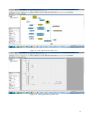
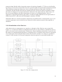
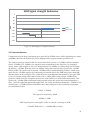
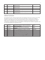
Undersökning och utveckling av multifilterbox
För mätningar på spurioser
Examensarbete inom högskoleingenjörsprogrammen Dataingenjör och Elektroingenjör
DAVID WAHLBERG
LUCAS WIMAN
Institutionen för Signaler och system
CHALMERS TEKNISKA HÖGSKOLA
Göteborg, Sverige 2014
Undersökning och utveckling av multi-filter box
För mätningar på spurioser
Examensarbete inom Högskoleingenjörsprogrammen Dataingenjör och Elektroingenjör
DAVID WAHLBERG
LUCAS WIMAN
© DAVID WAHLBERG & LUCAS WIMAN, 2014
Department of Signals and Systems
Chalmers University of Technology
SE-412 96 Göteborg
Sweden
Telephone +46 (0)31 - 772 1000
Foreword
We would like to thank Michael Johansson for the opportunity to work with this bachelor thesis. We
would also like to thank our supervisors, Göran Hult and Jörgen Ankarberg, who have helped us
during the work. Thanks to Samir Kilim and Martin Hedin for help with programming and
theoretical questions. We would also like to extend our thanks to Jonas Noreus for his help with
questions on how to write this thesis.
David Wahlberg & Lucas Wiman
Göteborg, 2014
Summary
This report describes the theoretical design of a flexible filter box for Ericsson at Lindholmen,
which purpose is to be able to be used in the measurement of spurious emissions, which are
unwanted interfering frequencies, outside radio frequency bands. The filter box needs, over a wide
frequency range, to amplify low power spurious emissions to make them measureable and attenuate
the carrier signal so the instruments used in combination with the filter box does not break. The
report describes the procedure of investigating viable components for the filter box which fits with
the requirements in terms of noise, size and cost of each component. These components were only
studied in theory using datasheets and information from distributors as it would be very expensive
to order them for the purpose of testing. The idea of using tuneable filters as components for the
filter box in order to cover a wider variety of frequency bands and lower the amount of necessary
filters was looked into. Based on the investigation of noise and size a filter box configuration was
developed. In theory it meets the noise, size and intermodulation requirements; however the amount
of intermodulation, a form of distortion in passive non-linear elements, from all components cannot
be determined in theory and could therefore be incorrect. An application written in the
programming language Agilent VEE was developed to add the possibility of controlling the filter
box with a computer. However, since there were no actual physical components to test with the
application the use of stubs was required, stubs are replacements for real components to simulate
the components behaviour. As a result, the application itself requires further development so it can
integrate with physical components. In addition, the outline of an automatic measurement algorithm
for the filter box was developed. The algorithms purpose is to ensure instruments do not break
during measurements using the filter box.
Abstract
Den här rapporten beskriver den teoretiska designen av en flexibel filterbox för Ericsson
Lindholmen vars syfte är att användas för mätningar av spurioser, som är oönskade störande
frekvenser utanför radiofrekvensband. Filterboxen måste, över en vid frekvensräckvidd, kunna
förstärka svaga spurioser för att göra dem mätbara, samt att dämpa bärvågen så att instrumenten
som används tillsammans med filterboxen inte går sönder. Rapporten beskriver de tillvägagångsätt
som använts för att undersöka om komponenter för filterboxen klarar de brus-, storlek- och
kostnadskrav som ställts. Komponenterna studerades enbart i teori med hjälp av datablad och
information från distributörer eftersom det hade varit för dyrt att beställa in alla komponenter och
testa dem. Idén med att använda filter med inställbar frekvens i filter boxen för att täcka så manga
frekvensband som möjligt, och samtidigt minska mängden filter som krävs för boxen har
undersökts. Baserat på undersökningarna av brus och storlek, utvecklades en filterboxkonfiguration
som teoretiskt sätt klarar brus-, storlek- och intermodulationskraven. Men mängden passiv
intermodulation, en typ av distortion i passiva icke-linjära element, från alla komponenter kunde
inte bestämmas med enbart teori. P.g.a detta så är intermodulationsfrågan fortfarande osäker. En
applikation, skriven med programspråket Agilent VEE, utvecklades för att lägga till möjligheten att
styra den tänkta filterboxen med en dator. Eftersom det inte fanns några fysiska komponenter att
testa med applikationen så fick stubbar användas, stubbar är ersättningskod för att simulera
komponenternas uppförande. Detta medför att applikationen behöver fortsatt arbete så den kan
integreras med framtida fysiska komponenter. Utöver programmet designades grunderna för en
automatisk styrningsalgoritm för filterboxen. Dess syfte är att försäkra att inga instrument eller
komponenter går sönder under mätningar med filterboxen.
Abbreviations
BW – Bandwidth
CW – Constant Wave
dBc – decibel in relation to carrier
DUT – Device under test
LNA – Low noise amplifier
IL – Insertion loss
IM – Intermodulation
OOB – Out-of-Band
PIM – Passive Intermodulation
RS – Requirement Specification
RX – Receiver
SEM – Spurious Emissions
SNR – Signal-to-Noise Ratio
TX – Transmitter
VR – Verification Report
VS – Verification Specification
Table of Contents
1. INTRODUCTION ......................................................................................................................................... 1
1.1 Background........................................................................................................................ 1
1.2 Purpose ............................................................................................................................. 2
1.3 Delimitations ...................................................................................................................... 2
1.4 Scope ................................................................................................................................ 3
1.5 Disposition ......................................................................................................................... 3
2. FRAME OF REFERENCE............................................................................................................................... 3
2.1 Theoretical terms ............................................................................................................... 3
2.2 Electronic components ....................................................................................................... 5
2.3 Agilent VEE........................................................................................................................ 8
3. PROCESS .................................................................................................................................................. 12
3.1 Collection of basic data .................................................................................................... 12
3.2 Fundamental theory ......................................................................................................... 12
3.3 Filter box design .............................................................................................................. 12
3.4 Agilent VEE Programming ............................................................................................... 24
4. RESULTS AND CONCLUSIONS .................................................................................................................. 31
4.1 Result .............................................................................................................................. 31
4.2 Discussion ....................................................................................................................... 32
4.3 Future Work ..................................................................................................................... 32
REFERENCES................................................................................................................................................. 33
APPENDICES................................................................................................................................................... 1
Appendix A: Filter box requirement specification...................................................................... 1
Appendix B: Components and datasheets ............................................................................... 1
1. INTRODUCTION
This chapter contains the background, purpose, delimitations and the scope of the project.
1.1 Background
Ericsson uses filters for verification measurements on radio units to radio base stations. At the
product verification section, specific filter boxes are used for measurements on different radio bands
which make their setup and configuration trivial. However, at the design/integration section these
measurements take a lot of time, each set of measurements can take hours to setup and calibrate and
they are extremely sensitive to external influence and the position of the cables. Switching from one
radio unit to another could lead to the failing of the measurement setup, resulting in several hours of
work being spent setting up the measurement again. A way to possibly avoid this problem would be
the development of a multi-filter box with several sets of filters, controlled by a computer (See
Figure 1).
The product design section at Radio Design Center-Lindholmen is interested in a general multifilter box used for specific out of band measurements. As of currently, these kinds of measurements
are done at system verification. However, because of time constraints at product design, there are
occasions when there is no time to wait for system verification to do the measurements. Therefore,
it would be of interest for the product design section to have their own filter box for measurements.
1
Figure 1: Early sketch of filter box
1.2 Purpose
The purpose of this report is to determine if it is possible to create a flexible filter box for
verification measurements on radio units for radio base stations. The filter box should be able to
attenuate a carrier signal to a level where a spectrum analyser can measure very weak signals outof-band, and also amplify spurious emissions, the very weak signals, in case that they are
underneath the noise floor of the spectrum analyser. This investigation is meant to give a good
theoretical framework for the possibilities of physically constructing the filter box, should it be
proven reasonable. This includes costs, size and various component requirements for the filter box.
1.3 Delimitations
In-depth software simulations of the filter box will not be investigated due to cost and time
constraints. For the same reasons, the filter box will only be constructed in theory. The filter box’s
main purpose is to measure out-of-band spurious emissions; other applications may be possible, but
they are not the focus of the investigation.
2
1.4 Scope
This investigation shall determine the requirements for the various measurements and the
restrictions they put on the system used for measurement and the filter box. The filter box shall not
limit the system used for measurement, in terms of signal-to-noise ratio. Additionally, possible
components and layouts for the filter box will be investigated, with costs and limitations in mind.
Also, the graphical programming language Agilent VEE will be used to program a way to control
the planned filter box.
1.5 Disposition
This report is written with each title in the method chapter running in chronological order of what
was conducted. The result chapter covers the final result, discussion and possible future plans for
the project.
2. FRAME OF REFERENCE
This chapter describes various terms that may not be commonly known for the reader and provides
a better explanation.
2.1 Theoretical terms
This section describes various terms and theory used in the project.
2.1.1 Spurious emissions
Spurious emissions are unwanted radio frequencies outside the channel. The spurious emissions can
consist of harmonic emissions, parasitic emissions, intermodulation products and frequency
conversion products. Spurious emissions can appear in the bandwidth and outside of the bandwidth
of a band. [1]
3
2.1.2 S-parameters
S-parameters, which are also known as “scattering parameters”, are used to quantify how radio
frequency energy propagates through a multi-port network. S-parameters provide a means to
accurately describe the properties of more complex networks as “black boxes”. For example, when
a radio frequency enters on one port some part of the signal is reflected back out of the same port,
some of it “scatters” and propagates through other ports, some of it might become amplified and
some of it dissipates as heat or electromagnetic radiation. The S-parameters of a two-port network
are generally known as:
S11 = voltage reflection coefficient of the input port
S12 = reverse voltage gain
S21 = forward voltage gain
S22 = voltage reflection coefficient of the output port
These parameters are often placed within a matrix (see Formula 1). [2]
൤
ܵଵଵ
ܵଶଵ
ܵଵଶ
൨
ܵଶଶ
Formula 1: S-parameter matrix
These parameters are used to calculate gain, insertion loss, return loss etc. For this report the most
important S-parameters will be S11 and S21 which are used for insertion loss and gain.
2.1.3 Noise
In electronic circuits, there is thermal noise, which is generated from components in the circuit
when the components have a higher temperature than 0 Kelvin. [3] This noise will negatively affect
a signal, e.g. the signal from a radio transmitter.
Signal-to-Noise Ratio abbreviated “SNR”, is the ratio between signal and noise power and is
usually expressed in decibels. A high SNR is important to differentiate the signal from the noise. [4]
SNR is affected negatively by the Noise Factor of components; Noise Factor is the ratio of input
SNR to output SNR expressed in linear. Instead of Noise Factor, Noise figure is often specified for
components.
ܰ‫ ݁ݎݑ݃݅ܨ݁ݏ݅݋‬ൌ ͳͲŽ‘‰ሺܰ‫ݎ݋ݐܿܽܨ݁ݏ݅݋‬ሻ
Formula 2: Noise Figure to Noise Factor conversion
ܴܵܰௗ஻ ൌ ͳͲ Ž‘‰ଵ଴ ሺ
ܲ௦௜௚௡௔௟
ሻ ൌ ܲ௦௜௚௡௔௟ǡௗ஻ െ ܲ௡௢௜௦௘ǡௗ஻
ܲ௡௢௜௦௘
Formula 3: SNR in dB
2.1.4 Decibel-milliwatts (dBm)
Decibel-milliwatt (dBm) is a power measurement relative to 1 milliwatt, and is expressed as:
4
௉
‫ ݔ‬ൌ ͳͲ݈‫݃݋‬
ଵ௠ௐ
Formula 4: Watt to dBm
And
௫
ܲ ൌ ͳܹ݉ ‫Ͳͳ כ‬ଵ଴
Formula 5: dBm to Watt
Where P is the power in Watt and x is the power in dBm.
It is used to measure the absolute power because of its capability to express both large and small
values in a small form. dBm is used in radio, microwave and fiber optic work. [5]
0dBm equals 1mW, 30dBm equals 1W, 40dBm equals 10W and so on. Calculating power with dBm
is simple since most components specify parameters, such as insertion loss or gain, in dB. For
example, an amplifier with 20dB gain will amplify a 20dBm signal to 40dBm.
ʹͲ݀‫ ݉ܤ‬൅ ʹͲ݀‫ ܤ‬ൌ ͶͲ݀‫݉ܤ‬
In linear, using the same numbers: an amplifier with 100 gain will amplify a 0.1W signal to 10W.
ͳͲͲ ‫Ͳ כ‬Ǥͳܹ ൌ ͳͲܹ
2.1.5 Passive Intermodulation (PIM)
Passive intermodulation is a form of intermodulation distortion that produces interference in high
frequency circuits. This can for example affect the wanted signal from a radio transmitter by hiding
it or distorting it. Passive intermodulation occurs when two or more signals exist in a passive and
non-linear device or element. The signals meld and mix with each other, generating a completely
different signal. [6] The PIM level is related to the carrier power, an increase of 1dB carrier power
approximately results in a 3dB higher PIM level. [7]
2.2 Electronic components
This section describes the components used for this project.
2.2.1 Tuneable Filters
For the purposes of this project, all electronic filters will be categorised as high frequency
components. A tuneable filter allows the user to control a bandpass or bandreject filter by tuning
where to start rejecting or letting through desired frequencies. This can be controlled by turning a
small knob on the device or controlling the filter digitally, using an optional remote digital interface,
5
such as GPIB. [8]
2.2.2 Directional Coupler
Couplers are passive devices used to split a portion of the power travelling in one transmission line
out through another connection or port. The coupler is a four port device consisting of an input port,
an output port, a coupled port and an isolated port (See Figure 2). The main line is usually between
ports 1 and 2 and is suited to carry higher power levels while port 3 and 4 are better suited for lower
powers because they are intended to only carry a small proportion of the main line power. A coupler
does not have set ports, any port of the 4 can be the input port, resulting in the directly connected
port being assigned as the transmitted port, the adjacent port becomes the coupled port and the
diagonal port becomes the isolated port. [9] For example, a 10dB coupler (See Figure 3) attenuates
the power by 10db.
Figure 2: Directional coupler and ports
Figure 3: Directional Coupler
6
2.2.3 Switches
All switches this report refers to are electromechanical switches suited for RF and microwave
applications (See Figure 4). In this report it is assumed the reader has the basic knowledge of how a
switch works. However, the terms TTL and cut-off power circuit might come across as unfamiliar.
TTL logic stands for “transistor-transistor-logic” and is used to enable the status of the switch to be
controlled by the level of the TTL logic input. [10]
A cut off power circuit is an option on some switches that allows it to cut off the DC current on the
actuator after switching, thus saving energy. [11]
Figure 4: Revolver switch
2.2.4 GPIB
GPIB, also known as ”General Purpose Interface Bus”, is a bus developed by Hewlett-Packard in
the 1960s. It is used to connect and control programmable instruments and is widely used as a
standard worldwide. The control of the instrument can be implemented in different ways, either
with an external controller such as a GPIB-USB interface (See Figure 5) or a GPIB Plug-in
Controller card. [12]
7
Figure 5: GPIB-USB interface
2.3 Agilent VEE
Agilent VEE (Visual Engineering Environment) is a visual test programming environment used for
tests, measurement and instrument control applications (See Figure 6). The programming language
is graphical and flow driven. A developer can connect graphical high-level objects to each other
and the way these objects are connected controls the flow of the application.
8
Figure 6: Example VEE application
Objects are the components used to create an application in VEE. Every single object represents
programming lines and instructions used in more common programming languages, such as C or
Java. An object can, once it executes, do an assortment of functions, such as displaying a graph or
executing MATLAB script. In addition, a VEE program may contain user-defined objects, which
are objects the user has created. These user-defined objects can also contain several existing objects.
In the Agilent VEE programming environment an object can be shown in two different modes, Icon
view and Open view. Icon view is where the object is minimized to cover as little space as possible
on the screen, while the Open view is used to further inspect the object to get a better idea of what it
contains and its instructions (See figure 7).
Figure 7: Object views
9
When objects are connected, they create a "thread". Data flows between objects in packages called
"containers". The container can hold data in various forms. For example, the data can be a scalar
number, an array of 500 strings or simply nil, which is an empty container. As a container of data
arrives to the input pin of an object it is called "pinging" and when the container comes out at the
output pin of the object the output pin is activated. There can also be pins at the top and bottom of
an object. These pins are called the sequence input and sequence output pins. The sequence input
pin at the top of an object, if connected, holds the execution of an object until the pin receives an
empty container i.e. the sequence input pin gets pinged. The sequence output pin at the bottom of an
object, when connected, becomes activated once the object and all data propagation have finished
executing (See figure 8).
Figure 8: Object pins
The flow of data in Agilent VEE applications moves from left to right and then from top to bottom
from each object. In detail, it works the following way. First, the data input pins and sequence-in
pins, if connected, are pinged. Secondly, the object executes. Thirdly, the output pins are activated.
Fourthly, the data propagates from left to right. Finally, the sequence out pin is activated to show
that the object has finished executing and propagates an empty container from top to bottom. This
output pin does not always need to be connected to something, but can be used to make sure an
object starts to execute only after the sequence output pin has sent a container to the objects
sequence input pin. When an Agilent VEE program is running, if there is more than one thread in
the program, they will all execute at the same time.
Creating a user interface in Agilent VEE can be done by switching between panel and detail view
and specifying the properties of each object, if they are going to be used for the panel view. The
panel view represents the user interface and what the operator will be able to see once the
application is running (See figure 9 and 10). The user can control the program with various
graphical objects, representing knobs, sliders and buttons. Each object in the panel view has a
corresponding object in the detail view. [13]
10
Figure 9: VEE Application detail view
Figure 10: VEE Application panel view
11
3. PROCESS
This chapter describes the various methods and procedures used in the project.
3.1 Collection of basic data
First of all, research had to be made to develop a better understanding of the various measurements
which the filter box was supposed to be included in. To accomplish this, several reports were
studied. The documents were provided by supervisor Jörgen Ankarberg, who is working with
software and hardware integration at the product design section of Ericsson. These documents
consist of VS, VR and RS reports, which describe the requirements and the procedure for the tests.
For each frequency band it is of great importance that the transmission does not interfere with other
frequencies outside the specified bandwidth. The test case has different requirements depending on
the frequency band. [14] Ericsson measures spurious emissions for frequencies from DC up to
around 13 GHz. The requirement for the amount of spurious emissions can vary depending on the
band and what frequency interval that is being measured. Some intervals might have a stricter
requirement while others allow a more relaxed requirement. The strictest requirement is around 115 dBm which is a very small amount of allowed spurious emissions.
3.2 Fundamental theory
To be able to design the filter box, the necessary background theory was necessary to learn.
According to supervisor at Chalmers, Göran Hult, it is important to know how S-parameters work.
Jörgen Ankarberg at Ericsson noted the importance of noise and attenuation in regards to the filter
box, so these terms needed to be investigated. Another issue is so called passive intermodulation,
which is difficult to estimate without physical components. See the theoretic reference for more
information regarding “Passive Intermodulation”.
3.3 Filter box design
In order to make a filter box as general as possible, it will need to cover all frequency bands of
interest to Ericsson. The bands are located at very different frequencies; from as low as 700 MHz up
to 2700 MHz, therefore filters with many different frequency ranges will be required. Furthermore,
since the spurious emission measurements are conducted out-of-band, it will be necessary to
measure from 0 Hz up to as high as 12.75 GHz. The table below (Table 1), sent in an email from
Jörgen Ankarberg, represents various frequency bands tested at Ericsson.
12
Table 1: Bands and frequencies
He also mentioned that the more interesting bands for the spurious emission measurements are B1,
B3, B7, B8, B12 and B13. UL (uplink) corresponds to the receiver frequencies for that particular
band, while DL (downlink) is the transmitter frequencies.
To settle what was needed of the filter box, input from Ericsson was necessary to define the
requirements. A requirement specification was written based on those requirements (See Appendix
A). Various datasheets for filters were studied to determine if they fulfill the requirements for the
planned filter box. To make the filter box even more general, tuneable filters were investigated, as
they would allow sweeping across frequencies. Using tuneable filters would in theory allow for a
more general configuration that can be used for a wider variety of measurements, and not only the
OOB TX measurements which is the main purpose of the filter box. In addition, the total amount of
components needed for the filter box is likely to be reduced by using tuneable filters. All
components, which are going to be used for the planned filter box, will contribute with an amount
of noise and attenuation which will need to be calculated for the entire system. The cost for each
component will also need to be taken into account. As the final system configuration will need to be
reasonably sized, approximations on size had to be made. For the different components, contact was
established with manufacturers and distributors, in order to inquire about the prices and further
specification of the components.
3.3.1 Filter box specification
The requirements for the filter box were determined by discussing with the supervisor at Ericsson
and reading the various documents related to measurements. To be able to measure signals at 13
115dBm with a SNR of >5dB, the signal first needs to be amplified to -85 dBm or higher, as the
noise floor of the spectrum analyser used at the product design section is around -90dBm at a
resolution bandwidth of 100kHz. Additionally the PIM of components will have to be taken into
account so that the SEM from the DUT can be differentiated from the intermodulation (IM)
products caused by the filter box. The received constant wave can have an average power of up to
100W which is more than most components can handle. To prevent breaking any components, a
coupler will have to be used to lower the signal power to 10W or less before it enters the filter box.
All components should have an impedance of 50Ω to minimize reflections caused by unmatched
impedances. Frequencies measured vary from 0 Hz up to 12.75 GHz, with the relevant bands in the
700 MHz to 2700 MHz range.
Using the frequencies for the previously mentioned range, a set of three ranges were written down
(Table 2) in order to get a better perspective of the specifications needed for tuneable filters. The
start number was obtained using the band with the lowest starting frequency within that range,
while the stop number represents the highest frequency. The bandwidth (BW) is the minimum and
maximum bandwidths for the given range. A list of requirements for the filter box was specified
using the assumptions above. (See Appendix A for the filter box requirements)
Start
Stop
BW (Mhz)
699 960 10-35
1710 2170 45-75
2500 2690 70
Table 2: Possible filter ranges
3.3.2 Selecting filters
Using the table of possible filter ranges (Table 2), a number of different filters were found at K&L
Microwave. [15] Among these, tuneable band reject and bandpass filters were included. The
tuneable filters are able to sweep over frequencies while the non-tuneable ones cover specific
bandwidths. Many of the filter datasheets stated that they were able to be digitally controlled, which
according to Martin Hedin and Samir Kilim, at Ericsson, would work with Agilent VEE, but
instrument drivers would need to be written for the tuneable filters in order to control them as the
filters are not included in standard libraries of Agilent VEE. Instrument drivers are interfaces which
allow the instrument to be controlled remotely from the PC. [16]
The idea of using a separate bandreject filter for each band was discarded due to the following
reasons; Size, cost and inflexibility. Regarding size, it is of interest to keep the box as compact as
possible. Using one filter solely for the purpose of covering a single band significantly increases the
number of filters needed, compared to using a tuneable filter to sweep over frequencies, thus
covering several bands.
When it comes to cost, it is assumed more filters results in a higher cost, even though tuneable
filters are individually more expensive. Finally, the use of non-tuneable filters would result in a
configuration where the only variable part is the externally connected components; which decreases
flexibility of the filter box.
By looking at different data sheets for an assortment of tuneable filters, the tuneable notch filters
were also rejected as the sweeping range was too small, therefore many different filters would still
14
be needed. Furthermore, while the centre frequency is tuneable, the bandwidth is not, so it could not
match all bands within the sweeping ranges, for some bands it was too narrow, whereas for others it
was too wide. The bandwidth of the bands varies between 10MHz and 75MHz, while the 3dB BW
for the tuneable notch filters in the relevant frequency range varies between 6MHz and 27MHz, i.e.
to attenuate the carrier, more than 4 cascaded filters would be needed for a particular band.
With both types of notch filters out of the picture, tuneable bandpass was investigated. Sweeping
the bandpass filter outside of the band, with the band in the filters stopband, would allow for more
flexibility as it does not rely on the filter having a specific bandwidth. With this idea, and the much
wider frequency ranges of the bandpass filters, only a few filters would be needed to cover most, if
not all, bands in the requirement specification.
In addition to covering as many bands as possible, the filters also needed to fulfil the requirements
for stopband attenuation; attenuating the carrier so that the SEM can be measured by the spectrum
analyser, as well as being able to measure as close to the carrier as possible.
With a stopband attenuation of 50dB, enough to bring a 10W carrier down to 0.1mW, the tuneable
filters which were looked into should handle the first requirement if the filter is considered ideal.
However,in reality, no filter is ideal. Additionally a drawback with having the flexibility of tuning is
that the shape factor of a tuneable filter is not as good as a non-tuneable filter. The reason for this is
that tuneable filters as of currently have a lower order than normal non-tuneable filters. This affects
the stopband negatively and measuring close to the carrier might become a limitation. Regardless, it
was decided that using two tuneable filters, for 0.5-1GHz and 1.5-3GHz respectively, as a base for
the filter box and search for filters complimenting them.
Having covered all bands, except for two very low priority ones, within the range of both tuneable
filters, only three more filters would be needed for measurements in the full range of DC-13GHz; a
lowpass filter for DC-0.5Ghz (See Figure 11), a bandpass filter for 1-1.5Ghz (See Figure 12) and a
highpass filter for 3-13GHz (See Figure 13). Considering where the bands lie, each filter was
quoted to a manufacturer. The following were the specifications sent to the manufacturer, with
additional comments on why these specifications were requested:
All filters able to handle 10W CW.
This is the highest power components need to handle if a 10dB coupler is used.
Lowpass
Passband insertion loss: 0-500MHz 2dB
Stopband attenuation: 650-3000MHz 50dB
15
Figur 11: Requested Lowpass filter frequency response
The passband covers the frequencies up to the where the first tuneable bandpass filter operates, the
stopband has some margin up to 699MHz which is where band B12 starts.
Bandpass
Centre frequency: 1250MHz
Bandwidth: 500MHz
Passband insertion loss: 1000-1500MHz 2dB
Stopband attenuation: 0-920MHz 50dB
Stopband attenuation: 1600-3000MHz 50 dB
Figur 12: Requested Bandpass filter frequency response
Passband covers the frequencies between the tuneable filters’ range. The lower stopband includes
Band 8 uplink; however the filter is not steep enough to include the downlink of the band, which
stops at 960MHz. Upper stopband at 1600MHz leaves ample room for band 3 that start at 1710MHz.
Note that band 11 and 21 is inside the passband of this filter. These are the two bands previously
mentioned as low priority and are not critical for the main application of the filter box.
16
Highpass
Passband insertion loss: 3000-13000MHz 2dB
Stopband attenuatino: 0-2700 MHz 50dB
Figur 13: Requested Highpass filter frequency response
The passband covers the remaining frequencies up to 13GHz and the stopband works for all
relevant bands, the closest being the downlink of band 7 at 2690MHz.
The specifications sent covers all required bands for TX, but misses out on the RX of band 8), it
also includes all other bands except for 11 and 21. If measurements are to be made on those bands,
an external filter will have to be connected.
The specifications returned from the manufacturer matched the requested specifications, with the
exception of the highpass filter which had the following frequency response (See Figure 14):
Figur 14: Actual Highpass filter frequency response
Having the stopband at 2700MHz was not possible and was changed to 2500MHz; resulting in
support for B7, TX 2500-2570MHz and RX 2620-2690MHz, being excluded for frequencies over
3GHz without the use of an external filter.
17
3.3.3 Selecting amplifiers
According to supervisor Jörgen Ankarberg, it was likely for the filter box configuration to use an
amplifier in the signal path to make the signal readable. Typically an amplifier is placed first in a
cascaded system to increase SNR compared to amplifying at a later stage. However, for the filter
box, if the amplifier is placed so it amplifies the signal before the carrier is attenuated; the other
components would be destroyed. The spectrum analyser at Ericsson has a noise floor around 90dBm, to be able to measure SEMs as low as -115dBm they have to be amplified first.
Considering the signal is coupled by a 10dB coupler before entering the filter box, the SEMs are
down to -125dBm. Insertion loss and cables attenuate the signal further, resulting in a power around
-135dBm, depending on path and frequency. For a SNR over 5dB an amplification of 50dB or more
is required. To leave some room for error, an amplifier with 55dB gain was selected. The insertion
loss of the amplifier is relevant as it affects the attenuation; however the amplifiers found with
sufficient gain to fit the requirement had quite high insertion loss compared to amplifiers with lower
gain, so the insertion loss had to be accepted regardless.
3.3.4 Selecting switches
To choose the signal path through the filter box, high frequency switches are needed. By reading
excel-sheets with existing filter box configurations provided by Ericsson, a few options and
manufacturers were found. Four switches, two with six input ports and two with four input ports,
are required for the envisioned setup. These ports connectors should ideally match the connectors of
the components, ensuring that no loss of signal power due to mismatched connector types occurs.
Since the signal path through the box, regardless of frequency and power, passes all switches, they
need to handle the full frequency range, DC-13GHz, as well as 10W CW. An additional property to
consider is that PIM levels should be as low as possible. When investigating the control of switches,
Samir Kilim at Ericsson stated that the switches were able to be integrated with Agilent VEE to
allow digital control. Including TTL logic and cutoff power circuits would improve usability and
lower power consumption. He also noted that adding an indicator to the switch would help the
testers verify that the correct switch is activated. When contacting a seller on these matters, each of
the added attributes would increase the price of the switches, but even with all options selected it
would still be within reason.
3.3.5 Additional components
The use of couplers will be required for some measurements, but they will be connected to the input
port of the filter box. This makes it possible to use components with lower power handling than
100W, as the coupler attenuates the power of the signal before it enters the filter box.
An attenuator will be used with the automatic measure algorithm (presented in 3.4.4) to prevent the
spectrum analyser from breaking when tuning the filters. Additionally, according to Jörgen
Ankarberg, a test setup for spurious measurements in-band usually features a path with around
50dB attenuation, so having the choice of using an attenuator instead of an amplifier can be useful
to make the filter box more flexible, thus a 40-50dB attenuator will be included in the filter box.
To connect all components with each other, radio frequency coaxial cables are going to be used. In a
fixed setup like the filter box, semi-rigid cables can be useful. They generally offer better electrical
18
properties than flexible cables, but at the expense of not being formable. [17] Even so, the flexible
type has previously been used in filter boxes for specific bands at Ericsson and consequently should
offer satisfactory properties. Moreover, since no design and layout of the inside of the box is
confirmed, only the flexible kind will be considered as they can be used almost regardless of how
the inside is configured. It is important that the cables have the right connectors; hence they will
have to be specified after all other components are chosen so everything matches. Also of
importance is the PIM generated by the cables, it cannot be higher than the lowest requirement for
SEM from the DUT; otherwise the PIM might be mistaken for SEM.
Should the filter box, with the proposed components, be insufficient for a measurement, one or two
external components can be connected, one instead of a filter and one instead of the amplifier or
attenuator.
3.3.6 Visualisation of the filter box
After the decision on components was complete, a schematic of the filter box was created (See
Figure 15). A connection without a component between the two last switches is included in case no
gain is necessary for the measurements. Furthermore, Jörgen Ankarberg noted that it is good to have
the option of a straight path through the box, though the type of switches used can have a maximum
of six input ports so no such path exists between the first two switches. It is, however, possible to
connect a cable instead of an external component, thus the option of a non-modified path exist.
Figur 15: Filter box configuration
19
3.3.7 Noise and attenuation calculations
The noise figure of passive components is equal to their attenuation i.e. the attenuation is equal to
the insertion loss of each component. [18] Using this information together with the already provided
insertion loss and gain of the amplifier, the total attenuation and SNR of the selected components
can be calculated to examine if the components match the requirements. The cascaded attenuation
for the filter box is calculated with Friis formula for noise factor (See Formula 6):
‫ܨ‬௧௢௧௔௟ ൌ ‫ܨ‬ଵ ൅
‫ܨ‬ଶ െ ͳ ‫ܨ‬ଷ െ ͳ
‫ܨ‬௡ െ ͳ
൅
൅‫ڮ‬൅
‫ܩ‬ଵ
‫ܩ‬ଵ ‫ܩ‬ଶ
‫ܩ‬ଵ ‫ܩ‬ଶ ǥ ‫ܩ‬௡ିଵ
Formula 6: Friis formula for noise factor
Where Fn is the noise factor and Gn is the gain of a component. The attenuation of the box will vary
depending on the frequency; a higher frequency generally equals a higher attenuation. Cables can
have a large impact on attenuation, especially at high frequencies. Since cable lengths between
components are not known, no exact calculations can be made. Presented here are the best-case and
worst-case scenarios for unwanted attenuation without regards to cabling.
Best-case scenario: Frequency at 1-1,5GHz means the switches operate at their best insertion loss
(IL), 0.2 dB, while also allowing the use of the filter with the lowest IL, 0.3dB, the non-tuneable
bandpass filter.
‫ܨ‬஻௘௦௧ ൌ ͳǤͲͶ͹ͳ ൅
ଵǤ଴଻ଵହିଵ
ଵǤ଴ସ଻ଵିଵ
଴Ǥଽହହ
൅
ଵǤ଴ସ଻ଵିଵ
଴Ǥଽହହ‫כ‬଴ǡଽଷଷଷ
଴Ǥଽହହ‫כ‬଴Ǥଽଷଷଷ‫כ‬଴Ǥଽହହ‫כ‬଴Ǥଽହହ‫כ‬ଷଵ଺ଶଶ଻Ǥ଻଺଺
൅
ଵǤ଴ସ଻ଵିଵ
଴Ǥଽହହ‫כ‬଴Ǥଽଷଷଷ‫כ‬଴Ǥଽହହ
൅
ଵǤଽଽହଷିଵ
଴Ǥଽହହ‫כ‬଴Ǥଽଷଷଷ‫כ‬଴Ǥଽହହ‫כ‬଴Ǥଽହହ
൅
ൌ ʹǤͶͷͶͷ
Converting Noise Factor to Noise Figure:
ܰ‫ ݁ݎݑ݃݅ܨ݁ݏ݅݋‬ൌ ͳͲ݈‫ʹ݃݋‬ǤͶͷͶͷ ൌ ͵Ǥͻ݀‫ܤ‬
Worst-case scenario: Frequency at 13GHz results in the worst IL, 0.5dB, for the switches and using
the highpass filter, which is tied with the tuneable filters for the worst IL at 1dB:
‫ܨ‬ௐ௢௥௦௧ ൌ ͳǤͳʹʹͲ ൅
ଵǤଶହ଼ଽିଵ
ଵǤଵଶଶ଴ିଵ
଴Ǥ଼ଽଵଶ
൅
ଵǤଵଶଶ଴ିଵ
଴Ǥ଼ଽଵଶ‫כ‬଴Ǥ଻ଽସଷ
଴Ǥ଼ଽଵଶ‫כ‬଴Ǥ଻ଽସଷ‫כ‬଴Ǥ଼ଽଵଶ‫כ‬଴Ǥ଼ଽଵଶ‫כ‬ଷଵ଺ଶଶ଻Ǥ଻଺଺
൅
ଵǤଵଶଶ଴ିଵ
଴Ǥ଼ଽଵଶ‫כ‬଴Ǥ଻ଽସଷ‫כ‬଴Ǥ଼ଽଵଶ
൅
ଵǤଽଽହଷିଵ
଴Ǥ଼ଽଵଶ‫כ‬଴Ǥ଻ଽସଷ‫כ‬଴Ǥ଼ଽଵଶ‫כ‬଴Ǥ଼ଽଵଶ
൅
ൌ ͵Ǥ͸Ͷ͸ͷ
Conversion to dB:
ͳͲ݈‫͵݃݋‬Ǥ͸Ͷ͸ͷ ൌ ͷǤ͸ʹ݀‫ܤ‬
As seen by the equations, there is a notable difference in attenuation between best- and worst-case
even without taking the cabling into consideration. However, to investigate the cable influence on
attenuation, an average of 30cm cable between stages was assumed, which including input port to
the first switch and the last switch to output totals 210cm. Using the formula for attenuation
provided by cable manufacturer Huber+Sunher (See Formula 7):
20
‫݊݋݅ݐܽݑ݊݁ݐݐܣ‬ǣ ܽ ‫ ݂ כ‬଴ǡହ ൅ ܾ ‫ܤ݂݀ כ‬Ȁ݉
Formula 7: Attenuation formula
Where “f” is frequency in GHz and “a” and “b” are coefficients specified for the cable.
For the “SUCOFORM_141_CU” cables considered for the box:
ܽ ൌ ͲǤ͵ͷͷ
ܾ ൌ ͲǤͲͶ
At 0.5Ghz and 210cm :
ͲǤ͵ͷͷ ‫Ͳ כ‬Ǥͷ଴ǡହ ൅ ͲǤͲͶ ‫Ͳ כ‬Ǥͷ ൌ ͲǤʹ͹݀‫ܤ‬Ȁ݉
ʹǤͳ݉ ‫Ͳ כ‬Ǥʹ͹݀‫ܤ‬Ȁ݉ ൌ ͲǤͷ͸͹݀‫ܤ‬
At 13GHz and 210cm:
ͲǤ͵ͷͷ ‫Ͳ כ‬Ǥͷͳ͵଴ǡହ ൅ ͲǤͲͶ ‫ ͵ͳ כ‬ൌ ͳǤͺ݀‫ܤ‬Ȁ݉
ʹǤͳ݉ ‫ͳ כ‬Ǥͺ݀‫ܤ‬Ȁ݉ ൌ ͵Ǥ͹ͺ݀‫ܤ‬
In the worst case scenario of noise factor for the filter box the value is 5.62dB and the worst case
scenario for cables is 3.78dB. Adding these values gives a total of 9.4dB attenuation. Assuming the
filter box is receiving a signal of -115 dBm, it is then coupled by 10dB resulting in -125dBm. From
the components and cables the signal is further attenuated to -134.4dBm. At this point the signal
needs to be amplified in order to be distinguishable. The 55dB amplifier increases the signal to 79.4dBm, which is above the noise floor at -90 dBm. With these values the SNR can be established.
ܴܵܰௗ௕ ൌ ሺെ͹ͻǤͶሻ െ ሺെͻͲሻ ൌ ͳͲǤ͸݀‫ܤ‬
As can be seen from this calculation, the signal is 10.6 dB stronger than the noise at the worst case
scenario with a signal at -115 dBm and the total attenuation of 9.4 dB.
As noted above, these values are just to acquire an idea of what attenuation to expect from the
cabling and will most likely differ slightly when compared to reality.
Below is a graph displaying how the spurious emissions signal power changes as it passes through
the filter box. When the strictest spurious emissions signal strength is unmodified their level is at 115 dBm (See Figure 16).
21
SEM Signal strength behaviour
0
-20
-40
dBm
-60
-80
SEM
Noise floor
-100
-120
-140
-160
Figur 16: SEM Signal strength behaviour
3.3.8 Intermodulation
Components used in these calculations were specified at 43dBm carrier while calculations are made
at 40dBm, therefore the PIM levels will be slightly better compared to the specified level.
The weakest spurious emission that is to be measured has a power of -115dBm, and the strongest
carrier is 50dBm CW. 50dBm is too much for most components in the filter box, so coupling a
carrier with a 10dB coupler to lower its maximum power to 40dBm is needed while also lowering
the SEM to -125dBm. With the carrier at 40dBm, using cables and switches specified to -160dBc
PIM at 43dB CW would result in around -129dBm passive intermodulation products, which is too
much for the -125dBm signal to be consistently measurable due to the SNR being lower than 5dB.
Measurements on the strongest CWs would therefore need additional attenuation to lower the PIM
levels. In contrast, using cables and switches with -130dBc PIM would result in -99dBm PIM
products, which is not low enough to measure the weak SEMs even with further attenuation. This
leads to the -160dBc PIM components being required before the carrier has been attenuated by a
filter. After the signal has passed through a filter, the carrier should be attenuated to -10dBm or less,
which means a -130dBc PIM level should be more than sufficient for the remaining components,
see calculations below.
ͳͲͲܹ ൌ ͷͲ݀‫݉ܤ‬
݄ܶ݁‫ܤ݀Ͳͳݕܾ݈݀݁݌ݑ݋ܿݏ݈݅ܽ݊݃݅ݏ‬
ͶͲ݀‫ ݉ܤ‬ൌ ͳͲܹ
ͳͲܹ݈ܵ݅݃݊ܽ‫݄ܿݐ݅ݓݏݎ݋݈ܾ݄݁ܽܿܽ݃ݑ݋ݎ݄ݐݏ݁ݏݏܽ݌‬ǡ ‫ܯܫܲ݊݅݃݊݅ݐ݈ݑݏ݁ݎ‬
െͳ͵Ͳ݀‫ ݈ܾ݁ܽܿܯܫܲܿܤ‬՜ െͻͻ݀‫ݏݐܿݑ݀݋ݎ݌ܯܫ݉ܤ‬
22
െͳ͸Ͳ݀‫ ݈ܾ݁ܽܿܯܫܲܿܤ‬՜ െͳʹͻ݀‫ݏݐܿݑ݀݋ݎ݌ܯܫ݉ܤ‬
݈ܵ݅݃݊ܽ‫݂݋݉ݑ݄݉݅݊݅݉ܽݐ݅ݓݎ݁ݐ݈݂݄݅ܽ݃ݑ݋ݎ݄ݐݏ݁ݏݏܽ݌‬ͷͲ݀‫ܾ݀݊ܽ݌݋ݐݏ݄݁ݐ݊݅݊݋݅ݐܽݑ݊݁ݐݐܽܤ‬Ǥ
ͶͲ݀‫ ݉ܤ‬െ ͷͲ݀‫ ܤ‬՜ െͳͲ݀‫ ݉ܤ‬ൌ Ͳǡͳܹ݉
Ͳǡͳܹ݈݉ܵ݅݃݊ܽ‫݄ܿݐ݅ݓݏݎ݋݈ܾ݄݁ܽܿܽ݃ݑ݋ݎ݄ݐݏ݁ݏݏܽ݌‬ǡ ‫ܯܫܲ݊݅݃݊݅݊ݐ݈ݑݏ݁ݎ‬
െͳ͵Ͳ݀‫ ݄ܿݐ݅ݓݏܯܫܲܿܤ‬՜ െͳͶͻ݀‫ݏݐܿݑ݀݋ݎ݌ܯܫ݉ܤ‬
െͳ͸Ͳ݀‫ ݄ܿݐ݅ݓݏܯܫܲܿܤ‬՜ െͳ͹ͻ݀‫ݏݐܿݑ݀݋ݎ݌ܯܫ݉ܤ‬
3.3.9 Size calculations
After deciding on the components to use in the box based on technical attributes, such as IL and
gain, size was taken into account. Height, width and length of all components were noted and they
were regarded as blocks for the purpose of determining the total space required to fit them inside a
box. At first, they were simply considered to be arranged in accordance to the visualisation in
Figure 15, except with no space in-between components for air or cables.
Since all components are placed in one layer, the height is equal to the height of the tallest
component, which is the switch. (See appendix B for component specifications)
‫ݐ݄݃݅݁ܪ‬ǣ ͷͳǤͲͷͶ݉݉
For width, every stage was calculated separately and the highest value was used.
ܹ݅݀‫݄ܿݐ݅ݓݏ݄ݐ‬ǣ ͷͳǤͲͷͶ݉݉
ܹ݅݀‫ݏݎ݁ݐ݈݂݄݅ݐ‬ǣ ͹͵ ൅ ͳ͵͹ ൅ ͳʹǤ͹ ൅ ͳͻǤͲͻ ൅ ͹ͺǤ͹͸ ൌ ͵ʹͲǤͷͷ݉݉
ܹ݅݀‫ݏݎ݋ݐܽݑ݊݁ݐݐܽ݀݊ܽݏݎ݂݈݁݅݅݌݉ܣ݄ݐ‬ǣ ͵ͳǤͶͻ͸ ൅ ͶͳǤͳͷ ൌ ͹ʹǤ͸Ͷ͸݉݉
As seen from the calculations above, the filter widths give the total width of the layer.
The length was calculated by simply adding the lengths of the longest component in every stage,
resulting in:
‫݄ݐ݃݊݁ܮ‬ǣ ͸ͻǤ͵Ͷʹ ൅ ʹͶͻ ൅ ͸ͻǤ͵Ͷʹ ൅ ͸ͻǤ͵Ͷʹ ൅ ͳͶͳǤ͹ ൅ ͸ͻǤ͵Ͷʹ ൌ ͸͸ͺǤͲ͸ͺ݉݉
As shown by the calculations, placing the components in this manner results in a box with the
measurements of 51.054x320.55x668.068mm, yielding a total volume of 10,93 litres.
An existing filter box in the lab was measured to 220x450x650mm, or 64.35 litres. Since the
existing box is roughly 6 times as spacious, it was assumed the chosen components would most
likely fit in a similar case, even including cables and room for ventilation. Note that this
configuration does not have any power supply as it had not been looked into at this point, nor does
it include any controller for the switches. The existing box is mounted in a 19’’ rack, so keeping the
width the same would allow the new box to be easily fitted in the same type of rack. Worthy of note
23
is that the filter box in the lab protrudes a bit though the backside of the rack, which is 600mm deep.
According to Jörgen Ankarberg at Ericsson it is not a problem if the box protrudes a little, but
keeping the filter box within the rack dimensions is preferable.
3.3.10 Filter box cost
After establishing contact with manufacturers and distributors, the costs for the components were
written down and calculated. The prices will not be documented in the report as they are considered
confidential by Ericsson.
3.4 Agilent VEE Programming
This part of the method chapter covers the development of the user interface for the control of the
filter box. The application was written in the Agilent VEE programming language.
3.4.1 Learning the basics
The programming language Agilent VEE was studied by reading and solving problems in the form
of small exercises to teach the user how the basic functions work and what the language is capable
of. Experienced programmers of VEE were consulted at Ericsson in order to further understand the
language. In addition, the programming software and the exercises were provided by Ericsson.
3.4.2 Flowchart for the application UI
For the programming of the user interface, a flowchart was drawn in order to understand how the
flow of the application was going to work (See Figure 17). The user needs to be able to select which
band that is going to be used for the configuration. Additionally, the ability to change the
configuration of the filter box by choosing the signal path is necessary. This is done by selecting
which filter/external component to be used along with attenuation/gain/external components. Once
a configuration has been selected, the user is prompted if the configuration is correct. If confirmed,
the user is able to start the measurement. Otherwise, the user can make a new selection for the
configuration.
24
Figure 17: Flowchart for the application
3.4.3 Programming control for the filter box
With the help of the flowchart, a user interface application was developed for the filter box.
However, due to the fact that no physical filters were available to be programmed, stubs were
instead used. Stubs are stand-ins for not yet implemented modules in the code, which in this case
would be the filters, amplifiers and switches since there were no physical components to apply the
control to. In addition, a stub was used to simulate the start of a measurement. [19] The features of
this program are the ability to choose which filter and amplifier to be used for the signal path for the
measurement and the ability to tune the tuneable filters. All selectable components in the user
interface matches the ones discussed in previous chapters.
25
The picture below (Figure 18) shows the application running and what options that is available for
the user.
Figure 18: Filter box control interface
In the program, the user is able to select what band, filter and attenuation he wants to use for the
measurement from three dropdown menus. Compared to the flowchart in the previous section, these
options do not need to be chosen in a specific order. A picture with components, representing the
inside of the filter box, is used to inform the user where his selections take place in the filter box
marked with red arrows. To start a measurement, the user must have selected a band, a filter and
attenuation, if any, followed by pressing the “Select Configuration” button to confirm his choices.
When pressed, all options selected will be displayed in their respective labelled windows. The
selected band along with its start and stop frequency will be displayed in “Band”, “Start frequency”
and “Stop Frequency”. The selected filter will be displayed in the “Filter” window along with, if the
filter is tuneable, its tuneable centre frequency. Finally, the chosen attenuation or amplification will
be displayed in the “Gain” labelled window. The user is then prompted to confirm his selected
options for the measurement. If the user made a mistake or wishes to change the selection, selecting
“no” in the prompt allows the user to make new choices and then press “Select Configuration”
again. If the user is content with his selection; he selects “yes” and the “Start measurement” button
becomes activated, allowing the user to press it. The picture below (Figure 19) displays an example
of a user confirming a selected configuration.
26
Figure 19: Confirming a configuration
The different selections and options will now be explained in more detail. From the “Select Band”
dropdown menu, the user is able to choose between predetermined bands or if the user does not find
the choice he is looking for, he can select the “Custom” option from the dropdown menu, allowing
him to specify the start and stop frequency for the band he wants to measure. After pressing the
“Select Configuration” after selecting the “Custom” option, the user gets a prompt where he first
enters the starting frequency of the band, followed by a prompt for the stop frequency. The picture
below (Figure 20) shows an example of the user entering a start frequency for the custom band
selection.
27
Figure 20: Entering a custom band
The “Select attenuation/amplification” menu allows the user to choose between using an amplifier
of 55 dB, an attenuator of 40 dB, a straight signal line or simply an external component such as a
different amplifier or attenuator.
For the selection of filters, a vertical slider is used to let the user choose what filter that is going to
be used for the measurement. Two of the selectable filters are tuneable, when either is chosen and
confirmed with the “Select Configuration” button, the program will prompt the user to enter a value,
which sets the centre frequency for the tuneable filter. The picture below (Figure 21) shows a user
entering a value for the selected tuneable filter.
28
Figure 21: Selecting filter centre frequency
The ”Start measurement” button as of currently only shows a message box, informing the user that
the measurement will now start.
3.4.4 Outline for measurement algorithm
In addition of coding a basic user interface for the planned filter box, an outline for an automatic
switching during measurement algorithm was created. The purpose of this algorithm is to plan
future functionality for the application in VEE by allowing the program to control the tuneable
filters and the switching of signal paths in the filter box. If the application has an automatic
measurement function, it would allow the user to save time by allowing the program to do the
majority of the switching of components. As of currently, the application would require the user to
make several measurements while studying the spectral analyser and power meter to investigate
whether attenuation or amplification is required. This algorithm is planned to be used only when the
tuneable filters are used for a measurement. The picture below (Figure 22) depicts a flowchart of
how the measurement algorithm could work
29
Figure 22: Outline for measurement algorithm
In general, this algorithm is meant to ensure that the measurement for spurious emissions with the
filter box proceeds without breaking any of the equipment used for the measurement. This includes
switching on the attenuator or amplifier where it is needed during the measurement. Furthermore,
the algorithm makes sure measurement is conducted for all frequencies below and above the
selected band. The algorithm consists of two main branches, one where the tuned filter frequency is
below the start frequency of the band (Shown to the left in the picture) and one where the tuned
filter frequency is above the stop frequency of the band (Shown to the right in the picture).
When the tuned filter frequency is below the centre frequency of the band, the algorithm works in
the following way. First a test checks if the tuned filter frequency is close to the start of the band. If
it is not, it is determined safe to use the amplifier, then measure and lastly the tuneable filter
increases its frequency and repeats the test until the frequency is considered close to the band.
Once considered close to the band, the attenuator is switched to, circumventing the risk of breaking
the spectrum analyser should the tuned frequency be in-band. Following this, the algorithm reads
30
the current frequency to determine if it is in-band or not. If it is, the frequency is repeatedly lowered
until it is no longer in-band. The algorithm then switches to an empty signal path and the strength of
the signal is read, then it either lowers the frequency until it is no longer considered strong, or
switches on the amplifier and measures at the frequency if the signal is considered weak. Finally the
filter tunes to the band stop frequency. At this point the other main branch of the algorithm will start
running.
When the other branch of the algorithm starts running, the frequency of the filter is above the band
and a test checks whether or not the tuned frequency is close to the band from the upper side. If it is,
attenuation is switched on and another test keeps checking if the frequency is in-band and increases
the frequency until it is no longer within the band. Following this, the filter box switches to an
empty signal path and checks if the signal is strong or not. If it is, the frequency is increased until
the signal is no longer considered strong otherwise the algorithm jumps back to the check which
determines if the frequency is close to the band or not.
If the filter is tuned to a frequency far above the band, the filter box switches on the amplifier and
measures. Afterwards a test checks if the filter has tuned to its max frequency. If it has not, the
frequency is increased and measured until the test validates the frequency as max. Otherwise, the
measurement ends and the user make a new selection for the application.
4. RESULTS AND CONCLUSIONS
Presented in this chapter are the results of the research and work outlined in the process chapter.
The conclusions made are also included, as is the difficulties that were encountered during the
project. Possible future plans for development are also present in this chapter.
4.1 Result
The theoretical outline of a more general filter box with tuneable filters was designed. The filter box,
based on the choice of filters, is able to support spurious emission measurements for bands B1, B3,
B4, B12 and B13. However, for B8 only RX is supported due to the bandpass filter having an
inadequate lower stopband. Furthermore, because the highpass filter could not meet the
requirements for stopband frequency, support for B7 will require an external filter. From the noise
calculations the box is able to handle the requirement of a 5dB signal-to-noise ratio, even in a worst
case scenario. The calculations of the size proved that the box would be of acceptable size for
placement in a 19” rack.
When it comes to the cost of all so far established components, i.e. cables, switches, filters,
attenuator and amplifier, the price seems reasonable compared to the guidelines received from
Ericsson.
A basic user interface in Agilent VEE has been created which simulates the behavior of switching
between components and bands to measure. In addition, the outline of an algorithm for automatic
control during measurement using tuneable filters has been created.
31
4.2 Discussion
This section covers the discussion of the result and interesting topics.
It is possible that more environmental friendly components exist for creating this filter box but it
was not a matter we investigated very deeply. It is uncertain if these components would have
sufficient requirements. However, it can be something to investigate for future work.
Since the drawback from using tuneable filters results in worse shape factor, it might not be possible
to measure as close to the carrier as desired. Working around it by attenuating the signal more
results in worse SNR, which in many cases would make the SEM undistinguishable from the noise.
However, it is questionable if using non-tuneable filters for the box would be better. Since they are
not tuneable, a large amount of filters would need to be used if the same amount of bands is going
to be covered. And a higher amount of filters is guaranteed to increase the price and size of the filter
box. If more filters are the answer, using the existing filter boxes for separate bands is probably
better than building a bigger box with all filters.
Another problem is that it is hard to account for all passive intermodulation without having
components to test. PIM needs to be measured on a real system since it is dependent on how clean
connectors are and if they are thoroughly connected. In addition, only the switches and cables have
specified levels of PIM, consequently, intermodulation of the other components are unaccounted for
and would have to be investigated before purchase.
The dynamic range of a spectrum analyser can prevent measurements on the most extreme cases,
50dBm carrier and -115dBm SEM. Even with the carrier attenuated by 50dB down to 0dBm the
difference is 115dB, which might be too much for spectrum analysers to handle. Using filters with
better stopband attenuation alleviates this problem.
It is hard to determine how difficult it is to implement the automatic measurement algorithm in
Agilent VEE. It is possible the algorithm can be improved and adjusted and is likely to be changed
because of the shape factor issue.
Given more time it is possible that other component choices exist which fulfils the requirements and
are cheaper than the ones we have picked. Maybe it is possible to adjust the parameters of the
tuneable filters further, thus circumventing the shape factor issue.
4.3 Future Work
Investigate other components to provide support for B7 and TX of B8.
Further development of the Agilent VEE user interface application. Prepare its integration with
physical components and solve possible bugs.
Write a manual for the Agilent VEE user interface application.
Investigate if there are cheaper and/or better alternatives to components.
32
Investigate if there are better tuneable filters with better shape factor.
Investigate the intermodulation of the components.
REFERENCES
1. ”Spurious Emissions”, itu.int, 1997 [Online]. Available: http://www.itu.int/dms_pubrec/itur/rec/sm/R-REC-SM.329-7-199707-S!!PDF-E.pdf [22 May, 2014]
2. ”S-parameters”, microwaves101.com, 2014 [Online]. Available:
http://www.microwaves101.com/encyclopedia/sparameters.cfm [22 May, 2014]
3. B. Molin, ”Analog Elektronik”, Edition 1:6, Malmö: Studentlitteratur AB, 2001
4. D.M. Pozar, Microwave Engineering, 4th ed., Hoboken, NJ: Wiley, 2012
5. Dong. J, ”Network Dictionary”, Saratoga:Javvin Technologies, 2007. [E-book], Available:
books24x7
6. Poole. I, ”Passive Intermodulation, PIM Distortion”, radio-electronics.com, 2014 [Online].
Available: http://www.radio-electronics.com/info/rf-technology-design/passive-intermodulationpim/basics-tutorial.php. [22 May, 2014]
7. “PIM Power Levels – A Brief Tutorial “, Summitek Instruments, summitekInstruments.com 2014
[Online]. Available: http://en.youscribe.com/catalogue/tous/professional-resources/pim-powerlevels-a-brief-tutorial-532632 [11 June, 2014]
8. “Tuneable filters”, klmicrowave.com, 2007 [Online]. Available:
http://www.klmicrowave.com/tuneable.php [22 May, 2014]
9. Poole. I, “RF directional coupler basics tutorial”, radio-electronics.com, 2014 [Online]. Available:
http://www.radio-electronics.com/info/rf-technology-design/coupler-combiner-splitter/rfdirectional-coupler-design-basics-tutorial.php [22 May, 2014]
10. Huang. B, ”TTL Logic levels”, learn.sparkfun.com, 2014 [Online], Available:
https://learn.sparkfun.com/tutorials/logic-levels/ttl-logic-levels [2 June, 2014]
11. “RF Switch definitions & terminology”, ceiswitches.com, 2014 [Online]. Available:
http://www.ceiswitches.com/DEFINITIONS.html [4 June, 2014]
12. “History of GPIB”, ni.com, 2012 [Online]. Available: http://www.ni.com/white-paper/3419/en/
[22 May, 2014]
13. “Agilent VEE 9.32”, agilent.com, 2013 [Online]. Available:
http://cp.literature.agilent.com/litweb/pdf/5989-9833EN.pdf [22 May, 2014]
14. Verification specification for RUS and RRUS01 B2 B3 and B9 Transmitter Performance
15. ”K&L Microwave”, klmicrowave.com, 2007 [Online]. Available: http://www.klmicrowave.com/
[6 June, 2014]
16. ”Instrument Driver Overview”, agilent.com, 2008[Online], Available:
http://www.home.agilent.com/agilent/editorial.jspx?cc=SE&lc=eng&ckey=1461187&id=1461187
[5 June, 2014]
17. ”RF cables”, hubersuhner.com, 2014[Online], Available:
33
http://www.hubersuhner.com/en/Products/Radio-Frequency/Cables [5 June, 2014]
18. Stiles. J, ”Noise Figure of Passive Devices”, ittc.ku.edu, 2005 [Online]. Available:
http://www.ittc.ku.edu/~jstiles/622/handouts/Noise%20Figure%20of%20Passive%20Devices.pdf
[22 May, 2014]
19. ”Stubs and Drivers”, www.jmu.edu, 2007[Online], Available:
https://users.cs.jmu.edu/bernstdh/web/common/help/stubs-and-drivers.php [2 June, 2014]
Personal references
20. Jörgen Ankarberg, Ericsson
21. Samir Kilim, Ericsson
22. Martin Hedin, Ericsson
34
1
APPENDICES
Appendix A: Filter box requirement specification
This appendix contains the requirements for the filter box
Interfaces
The switches and tuneable filters in the box will be controlled by a PC connected by GPIB. The box
will have extra ports for connecting external components for other measurements to increase
flexibility. An output port for connecting a spectrum analyser to measure signals.
1.
Original
2.
Original
3.
Original
GPIB for communication between
filter box and PC.
Ports for connecting external
modules
Port for spectrum analyser
Base
Base
Base
Functional requirements for filter box
The filter box has to be able to measure TX OOB spurious emissions on bands B1, B3, B4, B7 and
B8. Support for band B12 and B13 is desired and, if possible, support for other bands as well.
Ideally the filters will be digitally tuneable to keep the number of filters needed low. In order for the
signal to be distinguishable, it is necessary for the PIM level generated by the components to be 130 dBm or less with a 40dBm carrier. This requirement makes it possible to measure signals at 115 dBm, which is the strictest requirement for OOB measurements, with a SNR of at least 5dB. To
cover all desired measurements, the ability to handle a constant wave of 10W is required. For
signals to be measurable by the spectrum analyser, the carrier needs to be attenuated by at least 50
dB by the filters. Otherwise the spectrum analyser will in all likelihood break due to the carrier
power. The filter box needs to be of reasonable size and cost if it is going to be of interest for future
development. A necessary amount of switches to accommodate the filters is required.
4.
5.
6.
7.
8.
9.
10.
Original
Original
Original
Original
Original
Original
Original
11.
12.
13.
14.
Original
Original
Original
Original
Support for bands: B1, B3, B4, B7 and B8
Support for Band B12 and B13
Support for other bands
Digitally tuneable filters
One port for output
External component support (filters etc.)
Support for measuring down to -115dBm
SEM level
SNR greater than 5 dB
Support for up to 10W CW
Reasonable size
Reasonable cost
Base
Wanted
Extra
Wanted
Base
Base
Base
Base
Base
Base
Wanted
2
15.
Original
16.
Original
17.
18.
Original
Original
19.
Original
Support for TX OOB spurious emission
measurements
Support for RX OOB spurious emission
measurements
Support for other measurements
Switches for switching between
filters/amplifiers
Support for switching to a signal path with
high attenuation.
Base
Wanted
Extra
Base
Base
Software requirements
The application will be written in Agilent VEE. The application will need to be able to select what
filters that are going to be used for the measurement. The ability to switch between different
amplifiers in the application is also required. The addition of preset configurations for different
band is desired, to simplify usage of the application. A graphical representation of the current
configuration would further increase user friendliness. A descriptive user manual is important so the
user can understand how the application works.
21.
Original
22.
Original
23.
24.
25.
26.
27.
28.
29.
Original
Original
Original
Original
Original
Original
Original
Adjustable frequency range (by switching
and/or tuning filter)
Adjustable amplification (by switching
amplifier)
Preset for bands: B1, B3, B4, B7 and B8
Preset for Band B12 and B13
Preset for other bands
Easy to use interface
Graphical representation of settings
User Manual
Application written in Agilent VEE
Base
Base
Wanted
Extra
Extra
Base
Wanted
Wanted
Base
1
Appendix B: Components and datasheets
The following list is a compilation of the components that was chosen to match the requirements
laid out in the filter box design chapter, as well as their datasheets if available. The filter
specifications were provided by Peter Perman, consequently no proper datasheets are included.
Component type
Lowpass filter
Highpass filter
Bandpass filter
Tuneable bandpass filter
Tuneable bandpass filter
Amplifier
Attenuator
Switch-6port
Switch-6port
Switch-4port
Switch-4port
Cables
Product name
7L120-510/T1500-O/O
11SH10-3000/T13000-O/O
13ED50-1250/T500-O/O
5BT-500/1000-5-N/N
5BT-1500/3000-5-N/N
AMF-7D-00101800-30-10P
47-40-33
H6P-140138
H6P-140139
H4P-140139
H4P-140139
SUCUFORM_141_CU
Manufacturer
K&L Microwave
K&L Microwave
K&L Microwave
K&L Microwave
K&L Microwave
Miteq
Aeroflex/Weinschel
Charter Engineering
Charter Engineering
Charter Engineering
Charter Engineering
Huber+Suhner
Lowpass filter: 7L120-510/T1500-O/O
3.0 dB Cut-off Frequency
Passband Insertion Loss (1-500 MHz)
Stopband Attenuation (650-3000 MHz)
Return Loss
Filter Size
Input Connector Type
Output Connector Type
510 MHz
0.9 dB
53 dB
14.0 dB (1.5:1 VSWR)
116.84 x 12.70 x 12.70 mm
SMA Female
SMA Female
Highpass filter: 11SH10-3000/T13000-O/O
3.0 dB Cut-off Frequency
Passband Insertion Loss (3000-13000 MHz)
Stopband Attenuation (2500 MHz)
Return Loss
Filter Size
Input Connector Type
Output Connector Type
3000 MHz
2.0 dB
50 dB
9.54 dB (2.0:1 VSWR)
44.45 x 25.40 x 12.70 mm
SMA Female
SMA Female
2
Bandpass filter: 13ED50-1250/T500-O/O
Centre Frequency
3.0 dB Bandwidth
Insertion Loss
Stopband Atten. (DC - 920 MHz):
Stopband Atten. (1600 - 3000 MHz):
Return Loss
Filter Size
Input Connector Type
Output Connector Type
1250 MHz
500 MHz
0.3 dB
50 dB
50 dB
11.7 dB (1.7:1 VSWR)
138.27 x 78.76 x 19.02 mm
SMA Female
SMA Female
Tuneable Band Pass Filter: D5BT-500/1000-5-O/O-GRI-LP
Passband (500-1000MHZ)
Bandwidth
Lower Stopband (0-450MHZ)
Upper Stopband(1200-3000MHZ):
2 dB
5% of fcenter
50 dB
50 dB
Size
249 x 137 x 50 mm
Input Connector Type
Output Connector Type
G
R
I
SMA Female
SMA Female
GPIB Digital Interface
24 VDC
Tuning By Infrared Sensor
Tuneable Band Pass Filter: D5BT-1500/3000-2-O/O-GRI-LP
Passband (1500-3000MHz)
Bandwidth
Lower Stopband (0-1450MHz)
Upper Stopband(3105-6000MHZ):
2.7 dB
2% of fcenter
50 dB
50 dB
Size
187 x 73 x 50 mm
Input Connector Type
Output Connector Type
G
R
I
SMA Female
SMA Female
GPIB Digital Interface
24 VDC
Tuning By Infrared Sensor
3
Amplifier: AMF-7D-00101800-30-10P
Specifications at 23 °C
Frequency
Gain
Gain Flatness:
Noise Figure:
Noise Temperature:
VSWR In
VSWR Out
P1dB Out:
Voltage:
Current:
Outline Drawing:
Operating Temp:
0.1 to 18 GHz
55 dB min
2 dB+/- max.
3 dB max.
288.6 K max.
2.2:1 max
2.2:1 max
10 dBm min.
15 V nom.
425 mA nom.
121681
-40 to 75 °C
4
Attenuator: 47-40-33
5
Switches: H6P-140138, H6P-140139 and H4P-140139
6
7
Cables: SUCOFORM_141_CU
8