Download paper

Evaluating Continuous Probabilistic Queries Over
Imprecise Sensor Data
Yinuo Zhang1, Reynold Cheng1 , and Jinchuan Chen2
1
Department of Computer Science, The University of Hong Kong, Pokfulam Road, Hong Kong
{ynzhang,ckcheng}@cs.hku.hk
2
School of Information, Renmin University of China, Beijing, China
[email protected]
Abstract. Pervasive applications, such as natural habitat monitoring and locationbased services, have attracted plenty of research interest. These applications deploy a large number of sensors (e.g. temperature sensors) and positioning devices
(e.g. GPS) to collect data from external environments. Very often, these systems
have limited network bandwidth and battery resources. The sensors also cannot
record accurate values. The uncertainty of these data hence has to been taken
into account for query evaluation purposes. In particular, probabilistic queries,
which consider data impreciseness and provide statistical guarantees in answers,
have been recently studied. In this paper, we investigate how to evaluate a longstanding (or continuous) probabilistic query. We propose the probabilistic filter
protocol, which governs remote sensor devices to decide upon whether values
collected should be reported to the query server. This protocol effectively reduces the communication and energy costs of sensor devices. We also introduce
the concept of probabilistic tolerance, which allows a query user to relax answer
accuracy, in order to further reduce the utilization of resources. Extensive simulations on realistic data show that our method reduces by address more than 99%
of savings in communication costs.
1 Introduction
Advances in sensor technologies, mobile positioning and wireless networks have motivated the development of emerging and useful applications [5,10,22,7]. For example,
in scientific applications, a vast number of sensors can be deployed in a forest. These
values of the sensors are continuously streamed back to the server, which monitors
the temperature distribution in the forest for an extensive amount of time. As another
example, consider a transportation system, which fetches location information from vehicles’ GPS devices periodically. The data collected can be used by mobile commerce
and vehicle-traffic pattern analysis applications. For these environments, the notion of
the long-standing, or continuous queries [21,24,13,15], has been studied. Examples
of these queries include: “Report to me the rooms that have their temperature within
[15o C, 20o C] in the next 24 hours”; “Return the license plate number of vehicles in
a designated area within during the next hour”. These queries allow users to perform
real-time tracking on sensor data, and their query answers are continuously updated to
reflect the change in the states of the environments.
H. Kitagawa et al. (Eds.): DASFAA 2010, Part I, LNCS 5981, pp. 535–549, 2010.
c Springer-Verlag Berlin Heidelberg 2010
536
Y. Zhang, R. Cheng, and J. Chen
pdf (uniform)
pdf
(Gaussian)
temp.
reported by
sensor
temp.
o
25 C
o
26 C
uncertainty
region
(a)
o
27 C
location
Reported by
sensor
uncertainty
region
(b)
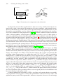
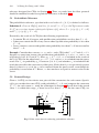
Fig. 1. Uncertainty of (a) temperature and (b) location
An important issue in these applications is data uncertainty, which exists due to various factors, such as inaccurate measurements, discrete samplings, and network latency.
Services that make use of these data must take uncertainty into consideration, or else
the quality and reliability may be affected. To capture data uncertainty, the attribute
uncertainty model has been proposed in [20,23,3], which assumes that the actual data
value is located within a closed region, called the uncertainty region. In this region, a
non-zero probability density function (pdf) of the value is defined, such that the integration of pdf inside the region is equal to one. Figure 1 (a) illustrates that the uncertain
value of a room’s temperature in 1D space follows a uniform distribution. In Figure 1
(b) the uncertainty of a mobile object’s location in 2D space follows a normalized Gaussian distribution. Notice that the actual temperature or location values may deviate from
the ones reported by the sensing devices. Based on attribute uncertainty, the notion of
probabilistic queries has been recently proposed. These are essentially spatial queries
that produce inexact and probabilistic answers [3,4,17,16,14,1].
In this paper, we study the evaluation of the continuous probabilistic query (or CPQ
in short). These queries produce probabilistic guarantees for the answers based on the
attribute uncertainty. Moreover, the query answers are constantly updated upon database
change. An example of a CPQ can be one that requests the system to report the IDs
of rooms whose temperatures are within the range [26o C, 30o C], with a probability
higher than 0.7, within the next two hours. Let us suppose there are two rooms: r1 and
r2 , where two sensors are deployed at each room and report their temperature values
periodically. At time instant t, their probabilities of being within the specified range
are 0.8 and 0.3 respectively. Hence, at time t, {r1 } would be the query answer. Now,
suppose that the temperature values of the two rooms are reported to the querying server
at every tP time units. Since their temperature values can be changed, the answer to the
CPQ can be changed too. For example, at time t + tP , the new probabilities for r1
and r2 of satisfying the CPQ are respectively 0.85 and 0.7. Then, the CPQ answer at
t+tP is {r1 , r2 }. We call the value 0.7, which controls the query answer, the probability
threshold parameter. This parameter allows a user to specify the level of confidence that
he wants to place in the query result.
A simple method for evaluating a CPQ is to allow each sensing device to periodically report their current values, evaluate the probabilities of the new sensor values, and
update the query result. This approach is, however, expensive, because a lot of energy
Evaluating Continuous Probabilistic Queries Over Imprecise Sensor Data
537
and communication resources are drained from the sensing devices. Moreover, when a
new value is received, the system has to recompute the CPQ answer. As pointed out in
[4], recomputing these probability values require costly numerical integration [4]. It is
thus important to control the reporting activities in a careful manner. In this paper, we
present a new approach of evaluating a CPQ, which (1) prolongs battery lifetime; (2)
saves communication bandwidth; and (3) reduces computation overhead. Specifically,
we propose the concept of probabilistic filter protocol. A probabilistic filter is essentially a set of conditions deployed to a sensing device, which governs when the device
should report its value (e.g., temperature or location) to the system, without violating
query correctness requirements [19,5]. Instead of periodically reporting its values, a
sensor does so only if this is required by the filter installed on it. In the previous example, the filter would simply be the range [26o C, 30o C], and is installed in the sensors in
r1 and r2 . At time t + tP , if the sensor in r1 checks that its probability for satisfying the
CPQ is larger than 0.7, it does not report its updated value. Thus, using the filter protocol, the amount of data sent by the devices, as well the energy spent, can be reduced.
Indeed, our experimental results show that the amount of update and energy costs is
saved by 99%. Since the server only reacts when it receives data, the computational
cost of re-evaluating the CPQ is also smaller.
We also observe that if a user is willing to tolerate some error in her query answer,
the performance of the filter protocol can be further improved. In the previous example,
suppose that the answer probability of room r1 has been changed from 0.85 to 0.65.
Since the probability threshold is 0.7, r1 ’s sensor should report its value to the server.
However, if the user specifies a “probabilistic tolerance” of 0.1, then, r1 can choose not
to report its value to the server. Based on this intuition, we design the tolerant probabilistic filter, which exploits the probabilistic tolerance. The new protocol yields more
energy and communication cost savings than its non-tolerant counterpart, by around
66%, in our experiments. We will describe the formal definition of probabilistic tolerance, and present the protocol details.
The rest of this paper is organized as follows. Section 2 presents the related work. We
describe the problem settings and the query to be studied in Section 3. Then we discuss
the probabilistic filter protocol in Section 4. The tolerant probabilistic filter protocol is
presented in Section 5. We give our experimental results in Section 6, and conclude the
paper in Section 7.
2 Related Work
In the area of continuous query processing, a number of approaches have been proposed to reduce data updates and query computation load. These work include: indexing
schemes that can be adapted to handle high update load [21]; incremental algorithms
for reducing query re-evaluation costs [24]; the use of adaptive safe regions for reducing update costs [12]; the use of prediction functions for monitoring data streams [13];
and sharing of data changes in multiple-query processing [15].
To reduce system load, researchers have proposed to deploy query processing to
remote streaming sources, which are capable of performing some computation. Specifically, the idea of stream filters is studied. Here, each object is installed with some
538
Y. Zhang, R. Cheng, and J. Chen
simple conditions, e.g. filter constraints, that are derived from requirements of a continuous query [19,5,22,11,25,8,7]. The remote object sends its data to the server only
if this value violates the filter constraints. Since not all values are sent to the server, a
substantial amount communication effort can be saved. In this paper, we propose the
use of probabilistic filters on data with attribute-uncertainty. To our best knowledge,
this has not been addressed before.
There also have been plenty of literature on probabilistic queries. [3] proposed a
classification scheme of probabilistic queries based on whether a query returns a numerical value or the identities of the objects that satisfy the query. Many studies focus
on reducing the computation time of probabilistic queries since such computing often
involves expensive integration operations on the pdfs [4,17].
However, most of the work on probabilistic queries focuses on snapshot queries queries that only evaluated by the system once. Few studies have addressed the issue of
evaluating CPQs. In [1], the problem of updating answers for continuous probabilistic
nearest neighbor queries in the server is studied. However, it does not explain how filters
can be used to reduce communication and energy costs for this kind of queries. In [9], a
tolerance notion for continuous queries has been proposed. However, it does not use the
attribute uncertainty model. In [2], we performed a preliminary study of using filters for
CPQs. We further improve this method by introducing the probabilistic tolerance, and
present an extensive evaluation on our approach.
3 Continuous Probabilistic Queries
In this section, we first explain the details of the system model assumed in this paper
(Section 3.1). Then, in Section 3.2, we present the formal definition of CPQ, as well as
a simple method of evaluating it.
3.1 System Model
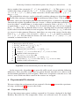
Figure 2 shows the system framework. It consists of a server, where a user can issue
her query. The query manager evaluates the query based on the data obtained from the
uncertain database (e.g., [3]), which stores the uncertainty of the data values obtained
from external sources. Another important module in the server is the filter manager. Its
purpose is to instruct a sensor on when to report its updated value, in order to reduce
the energy and network bandwidth consumption. In particular, the filter manager derives
filter constraints, by using the query information and data uncertainty. Then, the filter
constraints are sent to the sensors. The server may also request the filter constraints to
be removed after the evaluation of a CPQ is completed.
Each sensor is equipped with two components:
– a data collector, which periodically retrieves data values (e.g., temperature or position coordinates) from external environments.
– a set of one or more filter constraints, which are boolean expressions for determining whether the value obtained from the data collector is to be sent to the server.
Evaluating Continuous Probabilistic Queries Over Imprecise Sensor Data
Server
Sensors
error
model
Uncertain
Database
User
query
request
answer
update
539
sensor
value
Query
Manager
Filter
Manager
insert/delete
filter constraints
Filter
Data
Collector
Fig. 2. System Architecture
As discussed in Section 1, we use the attribute uncertainty model (i.e., a closed range
plus a pdf) [20,23] to represent data impreciseness. The type of uncertainty studied
here is the measurement error of a sensing device, whose pdf is often in the form of
the Gaussian or uniform pdf [20,23,3]. To generate the uncertain data, the uncertain
database manager stores two pieces of information: (1) an error model for each type
of sensors, for instance, a zero-mean Gaussian pdf with some variance value; and (2)
the latest value reported by each sensor. The uncertain data value is then obtained by
using the sensor’s reported value as the mean, and the uncertainty information (e.g.,
uncertainty region and the variance) provided by the error model. Figure 1 illustrates
the resulting uncertainty model of a sensor’s value.
In the sequel, we will assume a one-dimensional data uncertainty model (e.g., Figure 1(a)). However, our method can generally be extended to handle multi-dimensional
data. Let us now study how uncertain data is evaluated by a CPQ.
3.2 Evaluation of CPQ
Let o1 , ..., on be the IDs of n sensing devices monitored by the system. A CPQ is
defined as follows:
Definition 1. Given a 1D interval R, a time interval [t1 , t2 ], a real value P ∈ (0, 1], a
continuous probabilistic query (or CPQ in short) returns a set of IDs {oi |pi (t) ≥ P }
at every time instant t, where t ∈ [t1 , t2 ], and pi (t) is the probability that the value of
oi is inside R.
An example of such a query is: “During the time interval [1P M, 2P M ], what are the
IDs of sensors, whose probabilities of having temperature values within R = [10o C,
13o C] are more than P = 0.8, at each point of time?” Notice that the answer can be
changed whenever a new value is reported. For convenience, we call R and P respectively the query region and the probability threshold of a CPQ. We also name pi the
qualification probability of sensor oi .
At any time t, the qualification probability of a sensor oi can be computed by performing the following operation:
pi (t) =
fi (x, t)dx
(1)
ui (t)∩R
540
Y. Zhang, R. Cheng, and J. Chen
In Equation 1, ui (t) is the uncertainty region of the value of oi , and ui (t) ∩ R is
the overlapping part of ui (t) and the query region R. Also, x is a vector that denotes a
possible value of oi , and fi (x, t) is the probability density function (pdf) of x.
Basic CPQ Execution. A simple way of answering a CPQ is to first assume that each
sensor’s filter has no constraints. When a sensor’s value is generated at time t , its new
value is immediately sent to the server, and the qualification probabilities of all database
sensors are re-evaluated. Then, after all pi (t ) have been computed, the IDs of devices
whose qualification probabilities are not smaller than P are returned to the user. The
query answer is constantly recomputed during t1 and t2 .
This approach is expensive, however, because:
1. Every sensor has to report its value to the server periodically, which wastes a lot of
energy and network bandwidth;
2. Whenever an update is received, the server has to compute the qualification probability of each sensor in the database, using Equation 1, and this process can be
slow.
Let us now the probabilistic filter protocol can tackle these problems.
4 The Probabilistic Filter Protocol
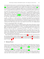
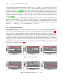
Before presenting the protocol, let us explain the intuition behind its design. Figure 3
shows a range R (the pair of solid-line intervals) and the uncertainty information of two
sensors, o1 and o2 , at current time tc , represented as gray-colored bars. Let us assume
that the probability threshold P is equal to one. Also, the current values extracted from
the data collectors of o1 and o2 are v1 (tc ) and v2 (tc ) respectively. We can see that o1 ’s
uncertainty region, u1 (tc ), is totally inside R. Also, v1 (tc ) ∈ u1 (tc ). Hence, o1 has a
qualification probability of one, and o1 should be included in the current query result.
Suppose that the next value of u1 is still inside R. Then, it is still not necessary for the
query result to be updated. More importantly, if o1 knows about the information of R
(the query region of a CPQ), o1 can check by itself whether it needs to send the update
to the server. A “filter constraint” for o1 , when it is inside R, can then be defined as
follows:
(2)
if u1 (tc ) − R = Φ then send v1 (tc )
R
R’’
R’
update at pi=0.7
Update at
pi<0.7
Update
at pi<1
update unnecessary
o1
Fig. 3. Illustrating probabilistic filter constraints
o2
Evaluating Continuous Probabilistic Queries Over Imprecise Sensor Data
541
which means: “When v1 has a chance to be outside R, report v1 to the server”. Thus,
the server can first compute constraint 2 and send it to o1 . As long as constraint 2 is not
satisfied, no update is produced by o1 .
The above technique can be generalized to handle any probability threshold P . Let
us consider Figure 3 again, where P = 0.7. Suppose that o1 continues to move towards
the left boundary of R, such that a fraction of more than 0.3 of its uncertainty region
(shaded) lies outside R. At this point, v1 must be reported, so that the ID o1 can be
removed from the query result. This is equivalent to using constraint 2, except that R is
replaced by R . Here, R is derived by using the maximum amount of o1 ’s uncertainty
region allowed on the outside of R, which is equal to 0.3 of o1 ’s uncertainty region.
Figure 3 also shows that o2 is currently outside R. For P = 0.7, the following
constraint can be used:
if u2 (tc ) touch R then send v2 (tc )
(3)
When u2 touches R , it has a fraction of exactly 0.7 inside R. Upon receiving the
update from o2 , the server should insert o2 to the query result. Notice that while R
is outside R, the region R is enclosed by R. In general, for every CPQ with P , two
constraints are need, to handle the cases when a value’s uncertainty is outside or inside
R. An additional advantage of this approach is that a sensor does not need to compute its
qualification probability, which can be complicated for a sensor with low computational
power.
R
li
ri
pi=0.7
oi
uncertainty center
Fig. 4. Checking filter constraints at the sensor
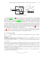
Simple Constraint Verification. In practice, a sensor may not keep the detailed uncertainty information to perform filter constraint checking. Also, since a sensor can have
low computational power, it is worthwhile to further simplify the constraint verification process. Observe that the uniform/Gaussian pdf assumed in our uncertainty model
has a symmetric shape, and is centered around the value sensed from the data collector
(c.f. Figure 1). It is then sufficient for the sensor to test the constraints by using only its
sensed value. Figure 4 illustrates a CPQ with P = 0.7. When the sensed value vi of
oi touches the line li , oi has exactly a qualification probability of 0.7. Thus, if vi is on
the left of li , its qualification probability must be less than 0.7. Similarly, if vi is on the
right of ri , its qualification probability is also less than 0.7. Hence, vi ∈ [li , ri ] if and
only if pi ≥ P .
542
Y. Zhang, R. Cheng, and J. Chen
The values of li and ri can be obtained by using the pdf information to derive the
distance from the boundaries of R. For uniform pdf, the distance can be obtained easily;
for Gaussian pdf, the value can be derived by performing table-lookup. This approach is
desirable for a sensor with low processing power. Moreover, only one interval ([li , ri ])
needs to be stored, as opposed to the two intervals presented earlier (e.g., R and R ).
Hence, the precious memory required by a sensor for storing the constraints is also
saved.
4.1 Protocol Design
We are now ready to discuss the probabilistic filter protocol. Algorithm 1 below shows
the algorithm employed by the server’s filter manager.
1
2
3
4
5
6
7
8
9
10
11
12
13
14
15
16
Initialization:
Request data from sensors o1 , . . . , om ;
for each sensor oi do
UpdateDB(oi );
Compute new filter constraint [li , ri ];
Send(addFilterConstraint, [li , ri ], oi );
Maintenance:
while t1 ≤ currentTime ≤ t2 do
Wait for update from oi ;
UpdateDB(oi );
if update == (oi , delete) then
remove oi from answer of Q;
if update == (oi , insert) then
insert oi to answer of Q;
for each sensor oi do
Send(deleteFilterConstraint, oi );
Algorithm 1. Probabilistic filter protocol (at filter manager)
In this algorithm, after a continuous query Q is registered, the server collects information from all sensors. Based on these values, the server evaluates the filter constraint
for each of them. Afterwards, the constraints are installed in the sensors (lines 2-6).
These constraints, in the form of [li , ri ], are computed by using the method described
in the previous section.
When Q is being executed (between times t1 and t2 ), the server continuously listens
to updates from all sensors. If it receives an update, it will update the uncertain database
(lines 9-10). Then, instead of recomputing the whole query answer of Q, an incremental
update approach is adopted: the server refreshes the query result according to the update
command received (lines 11-14). This is possible, because the update of oi only affects
its own qualification probability, but not other sensors. After the query is completed,
the filter constraints for query Q on all sensors are removed (Steps 15-16).
Evaluating Continuous Probabilistic Queries Over Imprecise Sensor Data
1
2
3
4
5
6
7
8
9
10
11
12
13
14
15
16
17
543
currState = FALSE;
while true do
command = receive(server);
switch command do
case addFilterConstraint
Add new filter constraint to oi ;
Stop;
case deleteFilterConstraint
Delete filter constraint from oi ;
Stop;
result = checkFilterConstraints(vi ,currState);
if result == include then
currState = TRUE;
sendUpdate(oi ,insert);
else if result == exclude then
currState = FALSE;
sendUpdate(oi ,delete);
Algorithm 2. Probabilistic filter protocol (at sensor)
Sensor side. Each sensor oi retrieves data value periodically from the external environment. It also uses a variable called currState to store its current state with respect
to Q: if oi is currently included in Q’s result, then currState has a true value, or
false otherwise. As shown in Algorithm 2, currState is initially FALSE (line 1).
The sensor then continuously listens to the commands from the server (lines 2-3). If the
server requests to add or delete filter constraints for a CPQ, it will do so accordingly
(lines 4-10). Then, it will check the filter constraints by using its latest sensed value vi ,
the currState value, and the checking method in the previous section (line 11). If oi
should be included in the query result, oi changes currState to TRUE, and notifies
the server (lines 12-14). Otherwise, oi is removed from the query result (lines 15-17).
These algorithms alleviate the problems of the basic protocol discussed in Section 3.2. At the sensor side (Algorithm 2), update is only sent to the server if the filter constraint is violated, not periodically. At the server side (Algorithm 1), since the
query answer is updated incrementally, there is no need to compute the qualification
probability of each sensor. Moreover, for both the server and sensors, no qualification
probabilities are computed. Hence, a significant amount of computational effort at both
the server and the sensors is reduced.
5 Tolerant Probabilistic Filters
In this section, we investigate how the performance of the probabilistic filter protocol
can be further improved, if the user is willing to sacrifice some degree of accuracy
(or equivalently, specify a tolerance) in her query answers. We present a definition of
544
Y. Zhang, R. Cheng, and J. Chen
tolerance designed for CPQs in Section 5.1. Then, we study how the filter protocol
should be modified in order to exploit this tolerance, in Section 5.2.
5.1 Probabilistic Tolerance
The probabilistic tolerance, specified with a real value Δ ∈ [0, 1], is defined as follows.
Definition 2. Given a CPQ Q, and Δ ∈ [0, min(P, 1 − P )], a Δ-CPQ returns results
S ∪ T at every time instant t during the lifetime of Q, where S = {oi |pi (t) ≥ P + Δ}
and T ⊆ {oi |pi (t) ≥ P − Δ}.
Essentially, the result of Δ-CPQ has the following requirements:
– It contain IDs of all sensors with qualification probabilities not less than P + Δ;
– It does not contain the ID of any sensor whose qualification probability is less than
P − Δ;
– It may contain a sensor with qualification probability less than P +Δ but not smaller
than P − Δ.
Example. Consider three sensors, o1 , o2 and o3 , and a CPQ with P = 0.7 and Δ = 0.1.
Suppose at some time instant, the qualification probabilities pi ’s of o1 , o2 , and o3 are
respectively 0.85, 0.55 and 0.71. Since p1 ≥ 0.7 + 0.1, o1 is included in the result of
this 0.1-CPQ. On the other hand, p2 < 0.7 − 0.1, and so o2 is excluded from the query
result. For o3 , its probability p3 is between [0.6, 0.8], and whether o3 is included in the
result does not affect the correctness of the query. Notice that if p3 was previously greater
than 0.8, there is no need for o3 to be removed from the query result, even though its
probability is now below 0.7. Hence, o3 does not have to report its newest value to the
server.
5.2 Protocol Design
Given a Δ-CPQ, we first derive two pairs of filter constraints for each sensor. Specifically, we consider the same CPQ, with probability P + Δ, and compute the constraint
[li+ , ri+ ] for each sensor oi , using the techniques in Section 4. Recall that if the sensed
value vi is within this range, pi must be no less than P + Δ. For the same CPQ, we
R
l i-
li+
ri+ ri
pi=P-ǻ=0.6
oi
pi=P+ǻ=0.8
Fig. 5. Filter constraints for enforcing probabilistic tolerance
Evaluating Continuous Probabilistic Queries Over Imprecise Sensor Data
545
derive another filter constraint [li− , u−
i ], for probability P − Δ. This means vi is located in this range, if and only if pi ≥ P − Δ. For example, in Figure 5, P = 0.7 and
Δ = 0.1. If vi ∈ [li+ , ri+ ], then pi must exceed 0.8. On the other hand, if vi ∈
/ [li− , ri− ],
then pi < 0.6.
The probabilistic tolerance can be enforced by making changes to Algorithms 1 and
2. For the filter manager (Algorithm 1), the maintenance phase (lines 7-16) is the same
as before, and so we only display the new initialization phase, as shown in Algorithm 3.
The main idea of this algorithm is that for a sensor oi whose qualification probability pi
is not less than P at initial time t0 , it only needs to report its value vi if its pi < P − Δ,
or equivalently, vi ∈
/ [li− , u−
i ]. In lines 5-6, all sensors of this type (R(t0 )) are assigned
−
−
the [li , ui ] filters. We say that this filter is active, meaning that it is currently employed
by the sensor to decide whether to send an update. The other filter, [li+ , u+
i ], is not used
(or inactive) in this moment. However, both filters are sent to the sensor. On the other
hand, if pi < P , then oi has to report vi when pi ≥ P + Δ, which is equivalent
+
+
−
−
to vi ∈ [li+ , u+
i ]. For this kind of sensors, the roles of the [li , ui ] and [li , ui ] are
switched, as shown in lines 8-11.
1
2
3
4
5
6
7
8
9
10
11
Initialization:
Receive data from all sensors o1 , · · · , om ;
Let R(t0 ) be the set {oi |pi (t0 ) ≥ P };
for each sensor oi in R(t0 ) do
+
+
Compute filter constraints [li− , u−
i ] and [li , ui ];
−
−
+
+
Assign [li , ui ] as active filter and [li , ui ] as inactive filter;
Send the 2 filter constraints to oi ;
for each sensor oi not in R(t0 ) do
+
+
Compute filter constraints [li− , u−
i ] and [li , ui ];
+
+
−
Assign filter [li , ui ] as active filter and [li , u−
i ] as inactive filter;
Send the 2 filter constraints to oi ;
Algorithm 3. New initialization phase for filter manager
At the sensor side, Algorithm 2 can generally still be used, except with the following
differences. First, two filter constraints are stored. Second, only the active filter is used
for determining whether to send an update. Third, once an update is sent, the active and
inactive states of the two filters stored in the sensors are swapped.
6 Experimental Evaluation
We now evaluate the performance of our protocols. Section 6.1 presents the experimental setup, and Section 6.2 discusses the results.
6.1 Experimental Setup
We use the temperature sensor readings captured by 54 sensors, deployed in the Intel
Berkeley Research lab. The temperature values are collected every 30 seconds. The
546
Y. Zhang, R. Cheng, and J. Chen
lowest and the highest temperature values are +13o C and +35o C respectively. So, we
set the domain space as +10oC to +40oC. The uncertainty region of a sensor value is
in the range of ±1o C [18], and we assume that uncertainty pdf is uniform. (We also
experiment with Gaussian pdf). We use 54 sensors to generate 155520 records over
one day, with a sampling time interval of 30s. For energy consumption, the energy for
sending an uplink message is 77.4mJ and the energy for receiving a downlink message
is 25.2mJ [6].
Each data point is obtained by averaging over the results of 100 random queries.
The size of each query is 5o C. The centers of the queries are randomly selected within
[12.5oC, 37.5oC]. All the queries has same duration as simulation period 1 day. By
default, P = 0.6. Since P cannot be 0 as stated in the definition, so in our experiment
we use P + where = 10−4 to substitute P = 0 case.
6.2 Experimental Result
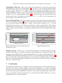
Probabilistic Filters. We first evaluate the effectiveness of introducing probabilistic filters. We focus on both communication cost and computation costs. From Figures 6(a)
and (b), the use of probabilistic filters reduce the update frequency and energy consumption rate by more than 99%. In detail, the average update frequency for probabilistic filters is around 0.074 per sampling interval, which is much less than when filters
are not used. The average energy consumption for the probabilistic filters is 7.6 mJ per
sampling interval. Moreover, using our protocol, the server does not need to do any
probability computation. Hence, the computational time for handling an update is also
significantly reduced (Figure 6(c)).
(a)
(b)
(c)
Fig. 6. Probabilistic Filters
(a)
(b)
Fig. 7. Probabilistic tolerance (P = 0.6)
(c)
Evaluating Continuous Probabilistic Queries Over Imprecise Sensor Data
547
Probabilistic Tolerance. Next, we evaluate the performance of our tolerant protocol,
under different values of Δ. From Figures 7(a) and (b) we can see that the improvement
is about a 66% reduction over update frequency and energy consumption (in maintainance phase), when Δ = 0.4. The reason for this improvement is that the increase
on the probabilistic tolerance gives more chances for sensors to avoid violating the constraints as well as sending updates. Figure 7(c) also shows that the computational time
on the server side is reduced by around 60% at Δ = 0.4. This is the consequence of
fewer updates received at the server.
0.08
update frequency
0.075
0.07
0.065
Variance=0.2
Variance=1
Variance=10
0.06
0.055
0.05
0
0.04 0.08 0.12 0.16 0.2 0.24 0.28 0.32 0.36 0.4
probabilistictoleranceǻ
Fig. 8. Probabilistic tolerance using Gaussian
distribution (P=0.6)
energyconsumptionper
samplinginterval(X103 mJ)
Gaussian Distribution. We also evaluate our protocol for uncertainty pdfs that follow
Gaussian distribution. Figure 8 shows that given the same tolerance value, more updates
are saved when the Gaussian pdf has a larger variance. For example, if Δ = 0.4, the
reduction using variance of 10 units over that of 0.2 units is around 20%. This reflects
that the filter constraints (e.g., li+ ) tend to be further away from the current sensed value
under a larger variance. Hence, our protocol works better for Gaussian pdf with a larger
variance.
90
80
70
60
50
40
30
20
10
0
50
100
# ofqueries
150
200
Fig. 9. Multiple Queries
Multiple Queries. Finally, we evaluate the performance of running multiple queries
in the system. We use a number of queries with random sizes and starting times. The
lifetime of each CPQ follows a uniform distribution of [2, 2880] sampling intervals. The
probability threshold and probabilistic tolerance are also randomly selected. In Figure 9,
we can see that the energy consumption rate scales linearly with the number of queries.
When we increase the number of queries, the increment on the energy per sampling
interval is around 438mJ.
7 Conclusions
Uncertainty management is an important and emerging topic in sensor-monitoring applications. In order to reduce update and energy consumption, we study a protocol
for processing continuous probabilistic queries over imprecise sensor data. We further
present the concept of probabilistic tolerance, and a protocol which enforces this tolerance, to yield more savings. In the future, we will study how other CPQs (e.g., nearestneighbor queries) can be supported.
548
Y. Zhang, R. Cheng, and J. Chen
Acknowledgments
Reynold Cheng was supported by the Research Grants Council of Hong Kong (Projects
HKU 513307, HKU 513508, HKU 711309E), and the Seed Funding Programme of the
University of Hong Kong (grant no. 200808159002). We would like to thank Prof. Kurt
Rothermel and Mr. Tobias Farrell (University of Stuttgart) for providing support on the
data simulator. We also thank the reviewers for their insightful comments.
References
1. Chen, J., Cheng, R., Mokbel, M., Chow, C.: Scalable processing of snapshot and continuous
nearest-neighbor queries over one-dimensional uncertain data. In: VLDBJ (2009)
2. Chen, J., Cheng, R., Zhang, Y., Jin, J.: A probabilistic filter protocol for continuous
queries. In: Rothermel, K., Fritsch, D., Blochinger, W., Dürr, F. (eds.) QuaCon 2009. LNCS,
vol. 5786, pp. 88–97. Springer, Heidelberg (2009)
3. Cheng, R., Kalashnikov, D.V., Prabhakar, S.: Evaluating probabilistic queries over imprecise
data. In: SIGMOD (2003)
4. Cheng, R., Kalashnikov, D.V., Prabhakar, S.: Querying imprecise data in moving object environments. IEEE Trans. on Knowl. and Data Eng. 16(9) (2004)
5. Cheng, R., Kao, B., Prabhakar, S., Kwan, A., Tu, Y.-C.: Adaptive stream filters for entitybased queries with non-value tolerance. In: VLDB (2005)
6. Crossbow Inc. MPR-Mote Processor Radio Board User’s Manual
7. Deshpande, A., Khuller, S., Malekian, A., Toossi, M.: Energy efficient monitoring in sensor
networks. In: Laber, E.S., Bornstein, C., Nogueira, L.T., Faria, L. (eds.) LATIN 2008. LNCS,
vol. 4957, pp. 436–448. Springer, Heidelberg (2008)
8. Elmeleegy, H., Elmagarmid, A.K., Cecchet, E., Arefs, W.G., Zwaenepoel, W.: Online piecewise linear approximation of numerical streams with precision guarantees. In: VLDB (2009)
9. Farrell, T., Cheng, R., Rothermel, K.: Energy-efficient monitoring of mobile objects with
uncertainty-aware tolerances. In: IDEAS (2007)
10. Gedik, B., Liu, L.: Mobieyes: Distributed processing of continuously moving queries on
moving objects in a mobile system. In: EDBT (2004)
11. Gedik, B., Wu, K.-L., Yu, P.S.: Efficient construction of compact shedding filters for data
stream processing. In: ICDE (2008)
12. Hsueh, Y.-L., Zimmermann, R., Ku, W.-S.: Adaptive safe regions for continuous spatial
queries over moving objects. In: Zhou, X., et al. (eds.) DASFAA 2009. LNCS, vol. 5463,
pp. 71–76. Springer, Heidelberg (2009)
13. Ilarri, S., Wolfson, O., Mena, E.: A query processor for prediction-based monitoring of data
streams. In: EDBT (2009)
14. Ishikawa, Y., Iijima, Y., Yu, J.X.: Spatial range querying for gaussian-based imprecise query
objects. In: ICDE (2009)
15. Li, J., Deshpande, A., Khuller, S.: Minimizing communication cost in distributed multi-query
processing. In: ICDE (2009)
16. Lian, X., Chen, L.: Monochromatic and bichromatic reverse skyline search over uncertain
databases. In: SIGMOD (2008)
17. Ljosa, V., Singh, A.K.: Apla: Indexing arbitrary probability distributions. In: ICDE (2007)
18. Microchip Technology Inc. MCP9800/1/2/3 Data Sheet
19. Olston, C., Jiang, J., Widom, J.: Adaptive filters for continuous queries over distributed data
streams. In: SIGMOD (2003)
Evaluating Continuous Probabilistic Queries Over Imprecise Sensor Data
549
20. Pfoser, D., Jensen, C.S.: Capturing the uncertainty of moving-object representations. In:
Güting, R.H., Papadias, D., Lochovsky, F.H. (eds.) SSD 1999. LNCS, vol. 1651, p. 111.
Springer, Heidelberg (1999)
21. Prabhakar, S., Xia, Y., Kalashnikov, D.V., Aref, W.G., Hambrusch, S.E.: Query indexing and
velocity constrained indexing: Scalable techniques for continuous queries on moving objects.
IEEE Trans. Comput. 51(10) (2002)
22. Silberstein, A., Munagala, K., Yang, J.: Energy-efficient monitoring of extreme values in
sensor networks. In: SIGMOD (2006)
23. Sistla, P.A., Wolfson, O., Chamberlain, S., Dao, S.: Querying the uncertain position of moving objects. In: Etzion, O., Jajodia, S., Sripada, S. (eds.) Dagstuhl Seminar 1997. LNCS,
vol. 1399, p. 310. Springer, Heidelberg (1998)
24. Xiong, X., Mokbel, M.F., Aref, W.G.: Sea-cnn: Scalable processing of continuous k-nearest
neighbor queries in spatio-temporal databases. In: ICDE (2005)
25. Zhang, Z., Cheng, R., Papadias, D., Tung, A.K.: Minimizing the communication cost for
continuous skyline maintenance. In: SIGMOD (2009)