1
UCRL-MA-130651
Reference Manual for the NUFT Flow
and Transport Code, Version 2.0
John J. Nitao
April 1998
ce re
n
re mo l y
w
r a r
La ive tion rato
L a o
N ab
L
DISCLAIMER
This document was prepared as an account of work sponsored by an agency of
the United States Government. Neither the United States Government nor the
University of California nor any of their employees, makes any warranty, express
or implied, or assumes any legal liability or responsibility for the accuracy,
completeness, or usefulness of any information, apparatus, product, or process
disclosed, or represents that its use would not infringe privately owned rights.
Reference herein to any specific commercial product, process, or service by trade
name, trademark, manufacturer, or otherwise, does not necessarily constitute or
imply its endorsement, recommendation, or favoring by the United States
Government or the University of California. The views and opinions of authors
expressed herein do not necessarily state or reflect those of the United States
Government or the University of California, and shall not be used for advertising
or product endorsement purposes.
UCRL-MA-130651
Reference Manual for the
NUFT Flow and Transport Code, Version 2.0
John J. Nitao
Earth and Environmental Sciences
Lawrence Livermore National Laboratory
April 1998
YMP9804051
Work performed under the auspices of the U.S. Department of Energy by Lawrence Livermore National Laboratory
under Contract W-7405-Eng-48. This work is supported by Yucca Mountain Site Characterization Project, LLNL.
Contents
Acknowledgments ...........................................................................................................................ii
1.
Introduction..............................................................................................................................1
2.
The Syntax of the Input Data...................................................................................................3
3.
How to Read the Input Documentation ...................................................................................8
4.
Basic Elements of the Input File............................................................................................11
5.
Input Data Documentation.....................................................................................................13
5.1
Mesh-Generation Parameters.......................................................................................14
5.2
Time-Stepping Parameters...........................................................................................22
5.3
Parameters for Numerical Methods.............................................................................24
5.4
Output Specifications...................................................................................................32
5.5
Specifying Initial Conditions.......................................................................................39
5.6
Setting Rock Properties ...............................................................................................41
5.7
Setting Source Terms...................................................................................................42
5.8
Specifying Boundary Conditions.................................................................................45
5.9
Other Options...............................................................................................................48
6.
Running Flow and Transport Sequentially............................................................................49
7.
References..............................................................................................................................50
Appendix A
Format of the Mesh File. .......................................................................................56
Appendix B
Numerical Algorithms Used..................................................................................58
Reference Manual for the NUFT Flow and Transport Code, Ver. 2.0
UCRL-MA-130651
i
Acknowledgments
The author wishes to thank the following organizations for supporting the documentation and
verification of the NUFT code: Waterways Experimental Station of the U.S. Army Corps of
Engineers, the Environmental Restoration Division at the Lawrence Livermore National
Laboratory (LLNL), the DOD/DOE Strategic Environmental Research and Development
Program (SERDP), and the DOE Yucca Mountain Project. The initial concepts of the code were
developed under the LLNL Institutional Research and Development program.
Preparation of this manual was made possible by the administrative assistance of Adrienne F.
Ridolfi and the editorial assistance of Karen L. Lew.
Reference Manual for the NUFT Flow and Transport Code, Ver. 2.0
UCRL-MA-130651
ii
1. Introduction
1. Introduction
NUFT (Nonisothermal Unsaturated-Saturated Flow and Transport model) is a suite of multiphase, multicomponent models for numerical solution of non-isothermal flow and transport in
porous media with application to subsurface contaminant-transport problems. These distinct
models are imbedded in a single code to utilize a common set of utility routines and input file
format.
Currently, the code runs on the Unix and DOS operating systems. Versions have been
successfully compiled and tested for IBM-PC compatibles, Cray Unicos, and the following
workstations: Sun, Hewlett-Packard, IBM Risc/6000, Silicon Graphics, DEC Alpha. Each set of
related models is called a module and has its own user’s manual that documents any particular
features and input data specific to that module. This reference manual for NUFT documents the
general numerical algorithms used and gives the documentation of the input to the model
common to all or most modules, including options not described in the user’s manual for each
module.
The following modules are available:
•
UCSAT—unconfined and confined saturated flow model
•
US1P—single-phase unsaturated flow (Richard’s equation)
•
US1C—single-component contaminant transport
•
USNT—NP-phase, NC-component with thermal option
It is recommended that new users of NUFT read the user’s manual (User’s Manual for US1
Module of the NUFT Code, Version 2.0, and User’s Manual for USNT Module of the NUFT
Code, Version 2.0) before reading this reference manual.
An integrated, finite-difference, spatial discretization is used to solve the balance equations. The
resulting nonlinear equation is solved at each time by the Newton-Raphson method. Options for
solution of the linear equations at each iteration are direct-banded solution and preconditionedconjugate gradient method with various preconditioning schemes.
The model can solve one-, two-, or three-dimensional problems. Future plans include
incorporation of capillary hysteresis, nonorthogonal mesh discretization, finite elements, and
nonlinear solid sorption isotherms.
The first stage of code verification with one-dimensional problems has been completed (Lee et
al., 1993) and further verification efforts were completed in 1998.
The distinct models in the code employ a common set of utility routines and input file format.
The various models are essentially isolated from each other; hence, future models can be added
without affecting existing models. This also allows for ease in code maintenance and
incorporation of future enhancements. Global variables in the code are virtually nonexistent. The
code is written principally in the C language. Input data is in the form of that used by the lisp
Reference Manual for the NUFT Flow and Transport Code, Ver. 2.0
UCRL-MA-130651
1
1. Introduction
language. An internal Lisp interpreter for the Scheme dialect of Lisp is part of the simulator
whose purpose is to read the input data file and the internal data files containing default input
data values. It also performs data checking.
Each module has its own user’s manual documenting the data input specific to each module.
Non-module-specific input are also given in the user’s manuals, but with only the most
commonly used input options covered. This reference manual describes the options for the nonmodule-specific data input in more detail and, also, describes the general numerical algorithms
used.
Reference Manual for the NUFT Flow and Transport Code, Ver. 2.0
UCRL-MA-130651
2
2. The Syntax of the Input Data
2. The Syntax of the Input Data
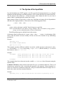
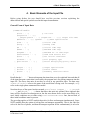
For each simulation run, NUFT requires a text file to specify the input parameters (e.g., the grid
definition and the hydrologic and fluid properties). This section describes the syntax of this file.
The file format is free format (i.e., it does not matter what column the data is in, nor does it
matter if data is continued past the current line or lines).
Input consists of lists of data blocks, or data units. Each data unit starts with a left parenthesis
and ends with a right parenthesis. A data unit is of the following general form:
(<name> <data> <data> . . .)
where
<name> refers to the input “variable” that is being set or specified
<data> are items that are real numbers, integer numbers, time real numbers, strings, pattern
strings, words, or other data units, or list(s) of data items.
The different data types are defined later in this section.
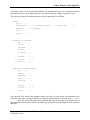
An alternate form for a data unit is (\<name> <data> <data> . . . \<name>). An advantage of this
form is that the model can more reliably tell the user the exact location of any unmatching
parentheses.
Example:
(porosity 0.2)
(file-name "input.data")
(par 0.1 0.3 0.6)
This example sets three different variables. It sets the variable porosity to the numeric value,
0.2, the variable file-name to the string, "input.data", and the variable par to a list of
three numeric values, 0.1 0.3 0.6.
Example:
(\rocktab
(silt (porosity 0.3) (Kx 1.e-4) (Ky 1.e-4) (Kz 1.e-4))
(sand (porosity 0.2) (Kx 1.e-2) (Ky 0.0) (Kz 0.0))
(clay (porosity 0.4) (Kx 1.e-6) (Ky 0.0) (Kz 0.0))
\rocktab)
This example shows how a data unit sets the variable, rocktab, to a list of data units using the
alternate form.
Comment Character: Semi-colons in the input file serve as comment characters. That is, all
characters on a given line after a semicolon are ignored by the program. Using comments is a
good way for the user to annotate an input file. Using two semicolons instead of a single one is a
good way to make sure that comments stand out.
Example:
(porosity 0.2) ;; this is how we set the value of porosity to 0.2
Reference Manual for the NUFT Flow and Transport Code, Ver. 2.0
UCRL-MA-130651
3
2. The Syntax of the Input Data
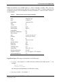
Units: All quantities are in MKS units (i.e., meters, kilogram, seconds). Thus, hydraulic
conductivities are in meters/second, and head is in meters (see Table 1). Unitless quantities such
as saturation, porosity, and concentrations are always fractional (i.e., between 0 and 1, inclusive),
not percentages.
Table 1.
Table of Units Used in Input to Models
length
mass
time†
temperature
area
volume
mass density
molar density
permeability
hydraulic conductivity
flow velocity
force
pressure
head
energy
specific energy
mass flux
molar flux
volumetric flux
energy flux
thermal conductivity
dynamic viscosity
molecular diffusivity
meters (m)
kilograms (kg)
seconds (s)
centigrade (°C)
m2
m3
kg/m3
mole/m3
m2
m/s
m/s
Newton (Nt=kg–m/s2 )
Pascals (Pa=Nt/m2 )
m
Joule (J=Nt–m)
J/kg
kg/s
mole/s
m3 /s
Watts (W = J/s)
W–m/°C
Nt–s/m2 =kg/m–s=103 centipoise
m2 /s
† model can accept other time units by the use of unit designators
Legal Data Types: Following are descriptions of valid data types:
•
A string —any sequence of visible characters delimited by double quotes “"”, for
example,
"hello there"
"run3-B (test#2)"
Note that spaces and parentheses are allowed in a string.
•
An integer number—for example, 11
Reference Manual for the NUFT Flow and Transport Code, Ver. 2.0
UCRL-MA-130651
4
2. The Syntax of the Input Data
•
A real number that is fixed or floating point—for example 1.23, –4.5e7, or
900.2E7. Note that D or d exponents in the manner of FORTRAN are not
allowed!
•
A time number that is a real number but that has the following unit designators as the
last letter to denote units of time. This type of number is used to specify a time.
s
seconds
m
minutes
h
hours
d
days
M
months
y
years
If no unit designator is present, “seconds” is assumed.
Examples:
20.0
23.1s
45e4M
20 seconds
23.1 seconds
45e4 months
There must be no spaces between the number and the unit designator.
•
A word—a sequence of nonblank, visible characters. A word can be a variable or may
be used in the same way as a string except that it cannot have internal blanks. The
model treats the words and strings as being distinct data types; the correct one, as
specified in the documentation, is required.
•
A pattern string —a special type of a string with the two unix shell-type “wild”
characters
* and ?
so that a pattern string can represent an entire class of strings that matches the string
pattern. The character * in a pattern matches any sequence of characters. Hence, the
pattern "*" matches all strings. The character ? in a pattern matches any single
character. Hence, the pattern "?" matches all strings with exactly one character.
Other Examples:
− The pattern "ex*" matches all strings that begin with the characters "ex".
− The pattern "ex*b2*z" matches all strings that begin with "ex", that are
followed by any number (including zero) of strings that are then followed by
the string "b2", and that end with the string "z".
− The pattern "r2?xay" matches all strings that begin with "r2", followed by
a single character, and that are then followed by the characters "xay".
Reference Manual for the NUFT Flow and Transport Code, Ver. 2.0
UCRL-MA-130651
5
2. The Syntax of the Input Data
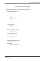
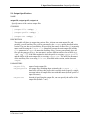
Include statement: The include statement is of the form
(include "<file-name>")
It is used to insert the contents of the file with the name "<file-name>" into the input file.The
file must lie in the working directory under which NUFT is being run. It can only be used to
replace a complete list (i.e., must be either a collection of data delimited by a closed set of
parentheses or a single data item such as a number or string). For example, if the file "data1.inc"
contains
(field (format list) (range "*") (variables Sl) (file-ext ".Sl")
(outtimes 0 70m 102m 222m 287m 342m 23h)
)
and the file "data2.inc" contains the single entry
200m
then the following input data
(output
(include "data1.inc")
(forcetimes (outtimes (include "data2.inc") 201m))
)
will be interpreted by the model as equivalent to
(output
(field (format list) (range "*") (variables Sl) (file-ext ".Sl")
(outtimes 0 70m 102m 222m 287m 342m 23h)
)
(forcetimes (outtimes 200m 201m))
)
The following is an example of an error. Suppose the file "file.inc" contains
(outtimes 0 70m 102m 222m
and the input file as the data item
(output
(field (format list) (range "*") (variables Sl) (file-ext ".Sl")
(include "file.inc") 287m 342m 23h)
)
(forcetimes (outtimes 200m 201m))
(file-ext ".Sl")
)
This is an error because only complete lists or a single entry can be included (not to mention the
fact that the parentheses will not match in the input file).
Include package statement: The include-pkg package statement is of the form
(include-pkg "<file-name>")
Reference Manual for the NUFT Flow and Transport Code, Ver. 2.0
UCRL-MA-130651
6
2. The Syntax of the Input Data
This statement is identical to the include statement except that it includes a file from the
subdirectory that contains the NUFT executable rather than a file from the current working
directory. The main purpose of the include package statement is to include a "package" of
predefined input parameters that comes with the NUFT software distribution
Macro commands: Macro commands start with the character "#". There are three commands
available: #define, #ifdef, and #ifndef. The following command defines a macro
variable,
(#define <variable>)
Currently, a variable cannot be defined to be any particular value; it is used in conjunction with
the other macro commands. The statements within
(#ifdef <variable> . . . .)
will be read as part of the input stream if <variable> is defined by the #define command.
However, the statements within
(#ifndef <variable> . . . .)
will not be placed as input if <variable> is not defined. The #define statements must be in the
same parenthesis level as, for example, bctab, genmsh, etc. The #ifdef and #ifndef
commands can be placed anywhere, except that the body of statements in the conditional
commands must be complete lists (i.e., parentheses match inside the macro command).
Currently, the macro commands only work inside an input set for a module or inside common.
Reference Manual for the NUFT Flow and Transport Code, Ver. 2.0
UCRL-MA-130651
7
3. How to Read the Input Documentation
3. How to Read the Input Documentation
The documentation of the input data to the code is written with special symbols that are not
actually part of the data input but that are used as convenient shorthand to mean certain things.
Following is a list of special symbols that are used:
•
Any word starting with the symbol < and ending with >
•
The symbols: ||
. . .
{ }
[ ]
The meaning of these symbols is given as follows:
•
Any italized word starting with the character < and ending with the character >
represents data, as described in the previous section, and will be called a data token (or
token, for short).
•
. . . is an abbreviation that means that more data items follow, but they are not
specified at this point; further explanation of the required missing data items will
follow.
•
[ ] means that data items inside [ ] are optional; for example, [ (xyz <real>) ] means
that the input value of variable xyz is optional.
•
|| represents a logical “exclusive or” of two sets of data items; for example,
(xyz <real>)||(abc <real>) means that the user must specify either the
variable xyz or abc but not both.
[ (xyz <real>)||(abc <real>) ] means that the user has the option of
either specifying xyz or abc.
•
{ } denotes a grouping of data items, usually used in conjunction with || ; for
example:
(xyz <real>)||{ (abc <real>) (ijk <integer>)} means that the user
must either specify xyz or specify both abc and ijk.
In the input documentation, the following data tokens have special meanings:
<string>
<integer>
<real>
<t-real>
<word>
<pattern>
a string
an integer number
a real number
a time real number; the last character is alphabetic and
denotes the units of time
a symbolic word
a pattern string
Reference Manual for the NUFT Flow and Transport Code, Ver. 2.0
UCRL-MA-130651
8
3. How to Read the Input Documentation
These data types are described in Section 2 of this reference manual.
Reference Manual for the NUFT Flow and Transport Code, Ver. 2.0
UCRL-MA-130651
9
4. Basic Elements of the Input File
4. Basic Elements of the Input File
Before going further, the user should have read the previous sections explaining the
abbreviations and special symbols used in this input documentation.
General Form of Input Data
(<name-of-model>
(title . . .)
;; run title
(outputfile . . .)||
{(output-prefix . . .) (output-ext . . .)};; output file name
(meshfile . . .)|| (genmsh . . .);;mesh specification
(time . . .)
;;initial time
(tstop . . .)
;;ending time
(dt . . .)
;;initial time step
(dtmax . . .)
;;maximum time step
(stepmax . . .)
;;maximum no. of time steps
(read-restart . . .)
;;read from restart file
(state . . .)
;;set initial conditions
(rocktab . . .)
;;soil property type
[ (grav-factor . . .) ]
;;factor multiplying gravity vector
[ (output . . .) ]
[ (srctab . . .) ]
[ (bctab. . .) ]
;;output specification
;;source tables
;;boundary condition tables
)
Recall that the “. . .” denote subsequent data items that are to be explained later and that all
of the input line past a semicolon is not read by the program but is for placing comments into the
input file. The above data units do not have to occur in any particular order. The data entry
<name-of-model> refers to the name of the model that is being used. For example, us1p
refers to the single-phase unsaturated flow model.
Note that the use of the square brackets around grav-factor, (output . . .), (srctab
. . .), and (bctab . . .) denote that these data units are optional. More optional data
items will be described in subsequent text, but the ones shown above are the most likely to be
used. Initial conditions are set either using read-restart or state. One, but not both, of
these initial conditions must be present.
The preceding applies to NUFT modules that solve for flow and transport simultaneously. Some
NUFT modules have the option of solving flow and transport sequentially. That is, the code first
solves for the flow of phases, and then the transport equation for the contaminant(s) is solved at
Reference Manual for the NUFT Flow and Transport Code, Ver. 2.0
UCRL-MA-130651
11
4. Basic Elements of the Input File
each major time cycle in an alternating fashion. (If transport takes place at a much shorter time
scale than does flow, the transport may take several time steps in a single, major time cycle.)
The form used when flow and transport are solved sequentially is as follows:
(common
(title. . .)
(outputfile . . .)||{(output-prefix. . .) (output-ext . . .)}
(meshfile . . .)||(genmsh . . .)
(time . . .)
(tstop . . . )
)
(<name-of-flow-model>
(dt . . .)
(dtmax . . .)
(stepmax . . .)
(state . . .)
(rocktab . . . )
[ (output . . .) ]
[ (srctab . . .) ]
[ (bctab . . .) ]
)
(<name-of-transport-model>
(dt . . .)
(dtmax . . .)
(stepmax . . .)
(state . . .)
(rocktab . . .)
[ (output . . .) ]
[ (srctab . . .) ]
[ (bctab . . .) ]
)
Note that the flow model and transport model each has its own initial and maximum time
steps and other data. Any input data that is common to both models are placed in the (common
. . .) data unit. Any of the items in the common data unit can also appear in the data unit of
the particular model, but they will be overridden by any specification that appears in the common
data unit.
Reference Manual for the NUFT Flow and Transport Code, Ver. 2.0
UCRL-MA-130651
12
5. Input Data Documentation
5. Input Data Documentation
The items in the input data file are classified in the following categories.
Mesh Generation Parameters
(genmsh . . .)
(mesh-file . . .)
Time Stepping and Numerical Solution Parameters
(time . . .)
(tstop . . .)
(dt . . .)
(dtmax . . .)
(stepmax . . .)
Output Specification
(title . . .)
(output . . .)
Specification of Initial Conditions
(state . . .)
(read-restart . . .)
Rock Property Specification
(rocktab . . .)
Source Term Specification
(srctab . . . )
Boundary Condition Specification
(bctab . . .)
Other options
(upstream-weighting . . .)
(include . . .)
Reference Manual for the NUFT Flow and Transport Code, Ver. 2.0
UCRL-MA-130651
13
5. Input Data Documentation: Mesh-Generation Parameters
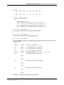
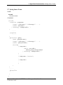
5.1 Mesh-Generation Parameters
NAME
genmsh
Internally generate a rectangular or cylindrical grid system
SYNOPSIS
(genmsh
(coord <coord-type>)
(down <num> <num> <num>)
(dx <numx-0> <numx-1> . . .)
(dy <numy-0> <numy-1> . . .)
(dz <numz-0> <numz-1> . . .)
(mat
(<el-name-prefix> <mat-type>
<i0> <i1> <j0> <j1> <k0> <k1>)
. . .
(<el-name-prefix> <mat-type>
<i0> <i1> <j0> <j1> <k0> <k1>)
)
[ (isot-dir) ]
[ (isot
(<num> <dir> <I0> <I1> <j0> <j1> <k0> <k1>)
. . .
(<num> <dir> <I0> <I1> <j0> <j1> <k0> <k1>)
) ]
[ (volfac
(<num> <I0> <I1> <j0> <j1> <k0> <k1>)
. . .
(<num> <i0> <i1> <j0> <j1> <k0> <k1>)
) ]
[ (areafac
(<num> <dir> <I0> <I1> <j0> <j1> <k0> <k1>)
. . .
(<num> <dir> <I0> <I1> <j0> <j1> <k0> <k1>)
) ]
[ (write-mesh "<file-name>") ]
[ (write-grid "<file-name>") ]
[ (write-gdef "<file-name>") ]
Reference Manual for the NUFT Flow and Transport Code, Ver. 2.0
UCRL-MA-130651
14
5. Input Data Documentation: Mesh-Generation Parameters
[ (gdef-ext "<file-ext>") ]
[ (non-log) ]
[ (wrap-around) ]
)
Reference Manual for the NUFT Flow and Transport Code, Ver. 2.0
UCRL-MA-130651
15
5. Input Data Documentation: Mesh-Generation Parameters
NAME
mesh-file
Allow user to easily generate a regular rectangular or cylindrical mesch (for more specific
meshes, see the mesh-file option)
PARAMETERS
(coord <coord-type>)
set type of coordinate system
<coord-type>
coordinate system type, options are
rect
cylind
(down <numx> <numy> <numz>)
sets the components of the vector pointing downward in the direction of
the gravity vector. The program will internally normalize the vector to
unity. Setting the components all to zero will turn off gravity in the model.
The vector is always with respect to a rectangular coordinate system
(X,Y,Z). For a rectangular mesh, the coordinate system coincides with the
rectangular coordinate system (x,y,z) of the mesh. If the mesh is
cylindrical, the vector is with respect to a coordinate system (X,Y,Z) where
X is the axis defined by θ = 0, z = 0; Y is the axis defined by θ = 90°, z = 0,
and the axis Z is defined by r = 0.
(dx <numx-0> <numx-1> . . .)
(dy <numy-0> <numy-1> . . .)
(dz <numz-0> <numz-1> . . .)
sets the mesh subdivisions in the x, y, and z coordinate directions.
Numbers that are repeated can be abbreviated; for example, 3*5.0 would stand for
three repeats of the numeral 5 (i.e., 5.0 5.0 5.0).
Reference Manual for the NUFT Flow and Transport Code, Ver. 2.0
UCRL-MA-130651
16
5. Input Data Documentation: Mesh-Generation Parameters
(mat
(<el-name-prefix> <mat-type>
<i0> <i1> <j0> <j1> <k0> <k1>)
. . .
(<el-name-prefix> <mat-type>
<i0> <i1> <j0> <j1> <k0> <k1>)
)
sets material property name of each element.
The element names will be of the form <el-name-prefix>#<i>:<j>:<k> where
<i>, <j>, <k> denote the i, j, and k indices. The material type <mat-type> is
defined in (rocktab . . .). The symbols nx, ny, and nz can be used
anywhere in place of numbers where an index is required. The model interprets
these to mean the number of subdivisions in the x, y, and z directions, respectively.
[ (isot-dir) ]
This parameter is optional. It affects the choice of the permeability (or hydraulic
conductivity) parameter. See the documentation of the permeability parameters K0,
K1, and K2 in subsequent text. This parameter should not be present for models
where isotropic permeability is desired.
[ (isot
(<num> <dir> <I0> <I1> <j0> <j1> <k0> <k1>)
. . .
(<num> <dir> <i0> <I1> <j0> <j1> <k0> <k1>)
) ]
sets isot = 0,1,2 in x,y,z directions, respectively; default is isot = 0 for all
elements. The parameter isot selects which of the permeability (or hydraulic
conductivity) values K0, K1, K2 set in rocktab are used for the particular
element.
[ (volfac
(<num> <i0> <i1> <j0> <j1> <k0> <k1>)
. . .
(<num> <i0> <i1> <j0> <j1> <k0> <k1>)
) ]
sets volume modifying factor. Multiplies the volume of the specified elements by
<num>
Reference Manual for the NUFT Flow and Transport Code, Ver. 2.0
UCRL-MA-130651
17
5. Input Data Documentation: Mesh-Generation Parameters
[ (areafac
(<num> <dir> <i0> <i1> <j0> <j1> <k0> <k1>)
. . .
(<num> <dir> <i0> <i1> <j0> <j1> <k0> <k1>)
) ]
sets area modifying factor
<dir>
valid options: x, y, or z;
dir = x will mult. the area between block i,j,k and i+1,j,k
dir = y will mult. the area between block i,j,k and i,j+1,k
dir = z will mult. the area between block i,j,k and i,j,k+1
[ (write-mesh "<file-name>") ]
write out mesh information using $con and $elc format
[ (write-grid "<file-name>") ]
write out mesh information using $freegrid format
[ (write-gdef "<file-name>") ]
write out minimal geometry information about the grid to file; the format of the grid
definition file is
$gdef
$type
<word> mesh type specified in coord
$nx
<real>
no. of subdivisions in x direction
$ny
<real>
no. of subdivisions in y direction
$nz
<real>
no. of subdivisions in z direction
$order <word> ordering of elements (e.g., xyz, yzx, or zxy
$dx
subdivisions in first coordinate
<real>
. . .
<real>
$dy
subdivisions in second coordinate
<real>
. . .
<real>
$dz
subdivisions in third coordinate
<real>
. . .
<real>
Line breaks are treated as significant in this format.
Reference Manual for the NUFT Flow and Transport Code, Ver. 2.0
UCRL-MA-130651
18
5. Input Data Documentation: Mesh-Generation Parameters
[ (gdef-ext "<file-ext>") ]
Write out minimal geometry information about the grid to file with file extension.
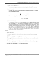
[ (non-log) ]
By default, flow areas in the radial direction for cylindrical coordinates are calculated
using the logarithmic formula.
A=
1
( ∆ r i − 1 + ∆ r i )∆θ∆z /ln(r i / r i − 1)
2
If the non-log flag is present, flow areas are calculated as
A = (r i − ∆ r i / 2)∆θ∆z
[ (wrap-around) ]
If <coord-type> is set to cylind, and the angles in the y (angular) direction sum to
360°, the elements at j = 1 are adjacent to corresponding elements at j = ny where ny is
the number of subdivisions in the y direction. When this option is present, the model
will make connections between these elements. This option is valid only for <coordtype> set to cylind. Default is no wrap-around. (Note that the wrap-around
option will increase the bandwidth of the matrix when using the direct-solution option
or the comb option of the preconditioned conjugate gradient method and, therefore,
will increase cpu time for these methods.)
NOTES
•
Indices start from 1.
•
Coordinates of grid blocks sides start from zero and are incremented by corresponding
values in
(dx . . .), (dy . . .), and (dz . . .).
•
The first grid block center in x direction has x = <dx0>/2, where <dx0> is the first number
in (dx . . .).
•
If coordinate type is cylind, the first coord x is radial distance, the second y is angle,
and third z is longitudinal to central axis.
•
The units of the angles in the cylind option are in degrees.
Reference Manual for the NUFT Flow and Transport Code, Ver. 2.0
UCRL-MA-130651
19
5. Input Data Documentation: Mesh-Generation Parameters
NAME
mesh-file
Specify name of mesh file
SYNOPSIS
(mesh-file "<file>")
DESCRIPTION
The user can set up a grid either by using the (genmsh . . .) option or by generating a
mesh file outside the program and then reading the mesh file into the NUFT model. The
genmsh option can only produce grids that are rectangular or cylindrical. The advantage of a
mesh file is that the user can write a program to generate the user’s own grid, taking full
advantage of the generality of the integrated, finite-difference method. The format of the mesh
file is described in Appendix A.
PARAMETERS
<file>
name of mesh file
Reference Manual for the NUFT Flow and Transport Code, Ver. 2.0
UCRL-MA-130651
20
5. Input Data Documentation: Mesh-Generation Parameters
NAME
grav-factor
Set gravity modification factor (optional), including gravity orientation (optional)
SYNOPSIS
(grav-factor <factor>)
DESCRIPTION
The user can optionally multiply the gravity vector in the model by this factor. (If the mesh-file
option is used, this factor is multiplied in addition to the beta factor read from the mesh file.)
By setting the factor to zero, gravity may be turned off. By setting this factor to the cosine of
the angle of inclination relative to the vertical downward direction assumed when creating the
mesh file, one can change the orientation of the model without rereading the mesh file. When
using the genmsh option, one can do the same thing through the down vector.
The default value is unity.
PARAMETERS
<factor>
real number multiplying gravitational acceleration
vector (default: 1.0)
Reference Manual for the NUFT Flow and Transport Code, Ver. 2.0
UCRL-MA-130651
21
5. Input Data Documentation: Time-Stepping Parameters
5.2 Time-Stepping Parameters
NAME
time, tstop, dt, dtmax, stepmax
Set automatic time-stepping parameters
SYNOPSIS
(time <t-real>)
(tstop <t-real>)
(dt <t-real>)
(dtmax <t-real>)
(stepmax <integer>)
DESCRIPTION
These input parameters are related to the automatic determination of the time-step size. Except
for stepmax, their values are <t-real> (i.e., time-real). The time-stepping algorithm that is
used is described in Appendix B. These parameters are required. Section 5.2.2 describes
optional parameters related to the automatic time-stepping and Newton Raphson iteration.
PARAMETERS
time
initial simulation time
tstop
simulation stopping time
dt
initial time step
dtmax
maximum time step allowed
stepmax
maximum number of time steps that, if exceeded, will halt the run
NOTES
The initial simulation time step overrides the time read in from a restart file if the restart
command is present. If the time command is not present, the time read in from the restart file
will be used.
Reference Manual for the NUFT Flow and Transport Code, Ver. 2.0
UCRL-MA-130651
22
5. Input Data Documentation: Time-Stepping Parameters
NAME
tolerdt, reltolerdt, dtmin
Set automatic time-stepping parameters (optional)
SYNOPSIS
(tolerdt <real> <real> . . .)
(reltolerdt <real> <real> . . .)
(dtmin <t-real>)
DESCRIPTION
These input parameters are related to the automatic determination of the time-step size at each
time step, as generated by the time-stepping algorithm. The algorithm seeks to control
maximum changes between the components of the solution vector from the current time step to
the next. The algorithm used is described in Appendix B.4.
PARAMETERS
tolerdt
maximum tolerance for change in components of solution vector from one
time step to the next
The data parameters are in the form (<variable> <real>) values, one for
each type of quantity in the solution vector. For example, for a model with
saturation and pressure in Pascals as the primary variables would have the
form
(tolerdt (S 0.5) (P 1.e5))
See the specific model documentation for specific details and the default
values.
reltolerdt maximum relative tolerance for change in components of solution vector from
one time step to the next
The data parameters are of the form of (<variable> <real>) values, one for
each type of quantity in the solution vector. For example, for a model with
saturation and pressure as the primary variables, in that order, the
following
(reltolerdt (S 0.5) (P 0.2))
dtmin
would seek to adjust the time step such that the saturation does not change
more than 10% nor the pressure more than 20% relative to the previous timestep values. The model will use the larger of the two time steps calculated
from the tolerdt and the reltolerdt values. See the specific model
documentation for specific details and default values.
minimum time step (default 0.0)
Reference Manual for the NUFT Flow and Transport Code, Ver. 2.0
UCRL-MA-130651
23
5. Input Data Documentation: Parameters for Numerical Methods
5.3 Parameters for Numerical Methods
NAME
tolerconv, reltolerconv, itermax, iterbreak, cutbackmax
Set parameters controlling Newton-Raphson iteration
SYNOPSIS
(tolerconv <real> <real> . . .)
(reltolerconv <real> <real> . . .)
(itermax <integer>)
(iterbreak <integer>)
(cutbackmax <integer>)
DESCRIPTION
Parameters controlling Newton-Raphson iteration (see Appendix B for description).
PARAMETERS
tolerconv
Maximum tolerance for change in components of solution vector from one
Newton-Raphson (NR) iteration to the next during a time step for NR
convergence criteria to be satisfied
The data parameters are of the form of (<variable> <real>) values, one
for each type of quantity in the solution vector. For example, a model with
saturation and pressure in Pascals as the primary variables, in that order,
would have the form
(tolerconv (S 0.5) (P 1.e5))
reltolerconv
See the specific model documentation for specific details and the default
values. Numbers that are repeated can be abbreviated; for example,
3*0.1 would stand for three repeats of the numeral 0.1 (i.e., 0.1 0.1
0.1).
Maximum relative tolerance for change in components of solution vector
from one NR iteration to the next for NR convergence
The data parameters are of the form of a list of nonnegative <real>
values, one for each type of quantity in the solution vector. For example,
for a model with saturation and pressure as the primary variables, in that
order, the following
(reltolerconv (S 0.5) (P 0.2))
would specify that NR convergence criteria is met if the saturation does
not change more than 10% and if the pressure changes no more than 20%
relative to the previous NR iteration values. The convergence criteria of
the model are satisfied if one or both of the tolerconv and
Reference Manual for the NUFT Flow and Transport Code, Ver. 2.0
UCRL-MA-130651
24
5. Input Data Documentation: Parameters for Numerical Methods
itermax
iterbreak
cutbackmax
reltolerconv criteria are satisfied. See the specific model
documentation for details and default values.
Maximum NR iterations
If exceeded (i.e., if NR convergence has not been reached, and the NR
iteration is greater than this number), the time-step size is cut back by
one-half, and the time step is started over (default value: 8).
Go on to next time step if this many NR iterations have been reached,
regardless of whether the NR convergence criteria are met (default value:
1000000000).
Maximum number of times in a given time step that the time step has to
be started over again due to lack of NR convergence
If exceeded, the program will print an error message and then stop
(default value: 100).
Reference Manual for the NUFT Flow and Transport Code, Ver. 2.0
UCRL-MA-130651
25
5. Input Data Documentation: Parameters for Numerical Methods
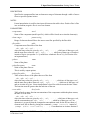
NAME
linear-solver, pcg-parameters
Set parameters for linear-solver
SYNOPSIS
(linear-solver <word>)
[ (pcg-parameters (precond <word>) (north <integer>)
(toler <real>) (itermax <integer>)
[ (direct <integer> <integer> . . . ) ]
) ]
[ (ilu-degree <integer>) ]
DESCRIPTION
These parameters are for the solution of linear system of equations that needs to be solved in
each iteration of the Newton-Raphson method.
Example:
(pcg-parameters (precond comb) (north 10) (toler 1.e-4)
(itermax 30) (direct 1 0))
PARAMETERS
linear-solver Sets the method used to solve the system of linear equations in the
Newton-Raphson method
Valid values are
lublkbnd standard ordered, constant bandwidth;
block-banded gaussian elimination (default)
vband
variable bandwidth elimination with reverse
cuthill-mckee bandwidth minimization
d4vband d4 ordered, variable bandwidth elimination
pcg
orthomin preconditioned conjugate gradient
method
(default value: blkbnd)
pcg-parameters
Parameters for preconditioned conjugate gradient (PCG) method
precond
Type of preconditioning method used
Options:
dkr
first degree incomplete ILU
ilu
incomplete ILU decomposition with variable fill-in
d4
incomplete ILU with d4 ordering with variable fill-in
comb
combinative method
Reference Manual for the NUFT Flow and Transport Code, Ver. 2.0
UCRL-MA-130651
26
5. Input Data Documentation: Parameters for Numerical Methods
bgs
block gauss-seidel method
none
no preconditioning
The recommended option for problems with linear or nearly linear
equations (e.g., ucsat) is
(pcg-parameters (precond bgs)
(toler 1.e-3) (itermax 500) (north 20))
For problems with intermediate nonlinearity (e.g., us1p, usnt), the
incomplete ilu of degree 0 (no fill-in) with generalized D4
ordering is recommended,
(pcg-parameters (precond d4) (toler 1.e-3)
(itermax 200) (north 15))
For problems with severe nonlinearities (e.g., usnt with phase
changes or highly nonlinear characteristic curves)
(pcg-parameters (precond d4) (toler 1.e-3)
(itermax 200) (north 15)) (ilu-degree 1)
The degree of incomplete LU decomposition is set by ilu-degree
to 1. Recall that the default is 0.
north
toler
Note that the D4 ordering is generalized, meaning that it also
works when connections between elements are nonstandard with
respect to the standard i,j,k lattice.
number of orthogonalizations performed in the orthomin PCG method
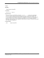
convergence tolerance for the PCG method
The convergence criteria is that the norm of the residual vector be less than
toler times the norm of the initial residual vector. The mean square
norm is used
|| r ||= (
1 n 2 1/ 2
∑ ri )
n i =1
maximum number of PCG iterations
If exceeded, the time-step size will be cut in half, and the time step will be
started over.
direct
specifies which of the balance equations are solved directly in the
combinative method used only for the (preconditioning option comb)
This is needed only for comb preconditioning method. Parameters are a list
of <integer>s, one for each balance equation. A nonzero value will cause
the linear equations for that balance equation to be solved directly by
gaussian elimination.
ilu-degree degree of fill-in for ILU decomposition
Degree 0 equals no fill-in.
itermax
Reference Manual for the NUFT Flow and Transport Code, Ver. 2.0
UCRL-MA-130651
27
5. Input Data Documentation: Parameters for Numerical Methods
NAME
time-method
Specify the time discretization method
SYNOPSIS
(time-method <string>)
DESCRIPTION
This parameter specifies whether to use either a fully implicit or fully explicit discretization in
time.
PARAMETERS
time-method
Valid values are "fully-implicit" or "explicit" (default value: model-specific).
Reference Manual for the NUFT Flow and Transport Code, Ver. 2.0
UCRL-MA-130651
28
5. Input Data Documentation: Parameters for Numerical Methods
NAME
upstream-weighting
Set upstream-weighting
SYNOPSIS
[ (upstream-weighting <weight>) ]
DESCRIPTION
sets upstream weighting
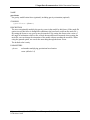
To calculate the advective flux cV of a component between two connected elements, the
model will use the weighting
c = acup + (1 − a)cdown
based on the weighting factor w where a= wLup/(wLup + (1–w)Ldown) where L refers to flow
lengths, the subscript up refers to upstream value, and the subscript down to downstream
value. The default is w=1, which is full upstream-weighting.
PARAMETERS
<weight>
weighting factor: usually between 0 and 1 inclusive (default: 1.0)
Reference Manual for the NUFT Flow and Transport Code, Ver. 2.0
UCRL-MA-130651
29
5. Input Data Documentation: Parameters for Numerical Methods
NAME
flux-correction, flux-correct-options
Set parameters controlling flux-correction scheme
SYNOPSIS
(flux-correction <word>)
(flux-correct-options (method <word>) (iter <integer>))
DESCRIPTION
By default, the model uses complete upstream-weighting of mobilities to numerically
calculate the advective flux between two elements (see upstream-weighting for
changing the amount of upstream-weighting). An alternative method is to use the fluxcorrection scheme of Smolarkiewicz [1983], which is a modification of the upstreamweighting. If flux-correction is set to on, the method of Smolarkiewicz is used with
three iterations. The number of iterations can be changed by setting parameters in fluxcorrect-options. An upstream, modified harmonic-averaging method can also be
used instead of the Smolarkiewicz.
PARAMETERS
flux-correction
can be set to either on or off to turn on flux-correction on or off
method
choice of flux correction method
smolark
flux-correction using Smolarkiewicz’s method
harmonic
flux-correction using harmonic averaging
iter
number of iterations for flux-correction
Using more than two iterations for the harmonic method can lead to spatial
oscillations in the solution. Using value of 1 for the harmonic appears to
give the same results as does the Smolarkiewicz method.
Reference Manual for the NUFT Flow and Transport Code, Ver. 2.0
UCRL-MA-130651
30
5. Input Data Documentation: Parameters for Numerical Methods
NAME
title
Set run title
SYNOPSIS
(title <string>)
DESCRIPTION
This input parameter specifies the run title, which is placed at the top of output files.
Example:
(title "Run 3A: hydrological study")
Reference Manual for the NUFT Flow and Transport Code, Ver. 2.0
UCRL-MA-130651
31
5. Input Data Documentation: Output Specifications
5.4 Output Specifications
NAME
output-file, output-prefix, output-ext
Specify names of the various output files
SYNOPSIS
[ (output-file <string>) ]
[ (output-prefix <string>) ]
[ (output-ext <string>) ]
DESCRIPTION
The model will place its output into various files. At least one main output file, and
possibly, several auxillary files, will be generated by the output option described in this
section. The user has two possibilities for specifying the names of these files: (1) separately
name each file using the output-file parameter to name the main output file and the
file parameter in output to name the auxilliary files; (2) more conveniently, have all
files use the same prefix (e.g., the run name), and use different suffixes for each file (e.g.,
“.out,” “.pg,” “.T”). If the latter method is used, the prefix is set using output-prefix,
and the suffix of the main output file is set using output-ext. The suffix for the names
of the auxilliary files is set using file-ext, described in this section, on the data unit
output.
PARAMETERS
output-file
output-prefix
output-ext
name of main output file
All output files, including those written by the (output . . . )
data field, will have this prefix; this is usually used to specify a single
run name where all output files start with this name (default: prefix of
input file name).
Instead of specifying the output file, one can specify the suffix of the
output file (default: “.out”).
Reference Manual for the NUFT Flow and Transport Code, Ver. 2.0
UCRL-MA-130651
32
5. Input Data Documentation: Output Specifications
NAME
output
Specify output
SYNOPSIS
(output
(field
[ (file "<file-name>") ]
(format <options>)
{(range "<element range>" . . .)||
(index-range (<i0> <i1> <j0> <j1> <k0> <k1>) . . .)}
(variables <el-var0> <el-var1> . . .)
(outtimes <t0> <t1> . . .)
)
(flux-field
[ (file "<file-name>") ]
(format <options>)
{(crange ("<element range>" "<element range>") . . .)||
(index-crange ((<i0> <j0> <k0> <i1> <j1> <k1>) . . .))}
(variables <con-var0> <con-i> . . .)
(outtimes <t0> <t1> . . .)
)
(history
(variable <el-var>)
(element "<element name>")
[ (file "<file-name>") ]
)
(flux-history
(variable <con-var0>)
(comp-flux (<comp> <phase>))}
{(connection "<element name>" "<element name >")||
(index-con <i0> <j0> <k0> <i> <j> <k>)}
[ (file "<file-name>") ]
)
(srcflux
(name <src-name>)
(comp <comp-name>)
[ (file "<file-name>") ]
(outtimes <t0> <t1> <t2> . . .)
Reference Manual for the NUFT Flow and Transport Code, Ver. 2.0
UCRL-MA-130651
33
5. Input Data Documentation: Output Specifications
[ (cumulative) ]
)
(bcflux
(name <bc-name>)
(comp <comp-name>)
[ (file "<file-name>") ]
(outtimes <t0> <t1> <t2> . . .)
[ (cumulative) ]
)
(forcetimes
(outtimes <t0> <t1> <t2> . . .)
)
(restart
[ (file "<file-name>") ]
(outtimes <t0> <t1> <t2> . . .)
)
(extool
(range "<element range>" . . .)||
(index-range (<i0> <i1> <j0> <j1> <k0> <k1>) . . .)
(variables <var0> <var1> . . .)
(outtimes <t0> <t1> <t2> . . .)
[ (file "<file-name>") ]
)
)
DESCRIPTION
Specifies the writing of various output data to files
Any of the preceding options can be specified; none of them is required.
PARAMETERS
(field
[ (file "<file-name>") ]
(format <options>)
{(range "<element range>" . . .)||
(index-range (<i0> <i1> <j0> <j1> <k0> <k1>) . . .)}
(variables <var0> <var1> . . .)
(outtimes <t0> <t1> <t2> . . .)
)
Outputs element data
Reference Manual for the NUFT Flow and Transport Code, Ver. 2.0
UCRL-MA-130651
34
5. Input Data Documentation: Output Specifications
(flux-field
[ (file "<file-name>") ]
(format <options>)
{(crange ("<element range>" "<element range>") . . .)||
(index-crange ((<i0> <j0> <k0> <i1> <j1> <k1>) . . .))}
{(phase-fluxes <phase0><phase1> . . .)||
(comp-fluxes (<comp0> <phase0>) (<comp1> <phase1>) . . .)}
(outtimes <t0> <t1> <t2> . . .))
)
Outputs flux output data
(history
(variable <var. name>)
(element "<element name>")
[ (file "<file-name>") ]
)
Specifies output of element variable vs. time
(flux-history
(phase-flux <phase>)||
(comp-flux (<comp> <phase>))
{(connection "<element name>" "<element name>")||
(index-con <i0> <j0> <k0> <i1> <j1> <k1>)}
[ (file "<file-name>") ]
)
Specifies output of flux variable vs. time
(srcflux
(name <src-name>)
(comp <comp-name>)
[ (file "<file-name>") ]
(outtimes <t0> <t1> <t2> . . .)
[ (cumulative) ]
)
Outputs the total instantaneous flux of a component, <comp-name>, due to a source term
set in srctab
The name of the source term <src-name> is the desired one in srctab. The sign
convention is such that flow out of the problem domain is positive, and flow out of the
domain is negative. If the statement [ (cumulative) ] is present, the cumulative flux
is outputted instead of the instantaneous flux. Note that cumulative fluxes are reset to 0 at
the beginning of a restart.
Reference Manual for the NUFT Flow and Transport Code, Ver. 2.0
UCRL-MA-130651
35
5. Input Data Documentation: Output Specifications
(bcflux
(name <bc-name>)
(comp <comp-name>)
[ (file "<file-name>") ]
(outtimes <t0> <t1> <t2> . . .)
[ (cumulative) ]
)
Outputs the total instantaneous flux of a component, <comp-name>, flowing into a set of
elements specified as boundary elements in bctab
The name of the boundary condition <bc-name> is the desired one in bctab. The sign
convention is such that flow out of the set of elements is positive, and flow into the
elements is negative. If the statement [ (cumulative) ] is present, the cumulative flux
is outputted instead of the instantaneous flux.
(forcetimes
(outtimes <t0> <t1> <t2> . . .)
)
Forces the model to hit specified times without necessarily outputting any information
This is used to prevent the model from skipping over the times at which fluxes or boundary
conditions change suddenly.
(restart
[ (file "<file-name>") ]
(outtimes <t0> <t1> <t2> . . .)
)
Write out a restart record at the specified times
Restart record can be read in as initial conditions using the restart command. Backup
restarts are also written (see subsection on reading restart information). The state
command must not be present when using this command.
(extool
(range "<element range>" . . .)||
(index-range (<i0> <i1> <j0> <j1> <k0> <k1>) . . .)
(variables <var0> <var1> . . .)
(outtimes <t0> <t1> <t2> . . .)
[ (file "<file-name>") ]
)
Outputs a ”time-history file“ in extool format program
NOTES
1. (outtimes <t0> <t1> <t2> . . .) can be replaced by either of the following:
Reference Manual for the NUFT Flow and Transport Code, Ver. 2.0
UCRL-MA-130651
36
5. Input Data Documentation: Output Specifications
a) (outtimes), which means all times
b) (triggers
((wake <state-var> (range "<el-name>" . . .) <op> <val>)
(cond <state-var> (range "<el-name>" . . .) <op> <val>))
. . .
((wake <state-var> (range "<el-name>" . . .) <op> <val>)
(cond <state-var> (range "<el-name>" . . .) <op> <val>))
)
which checks to see, at every time step, if any of the triggers goes off. A trigger goes off if
the condition v <op> <val> is true for the wake field where v is the value of the state
variable <state-var> at the elements with names in the range ("<el-name>" . . . ). If
this condition is true, the corresponding condition for the cond field is checked; if true,
then trigger goes off, and output occurs. Triggers only go off once.
(format <options>) : <options> can be any of following list or by-list list values and
element names (contsac format):
list
list values and element names
by-set
list values as a lisp vector, [ #n v1 v2 . . . vn ]
by-x
list x coord. and value
by-y
list y coord. and value
by-z
list z coord. and value
by-xyz
list x, y, z coordinates and values
by-ijk
list i,j,k index and value
by-xtable
format compatible with state using by-xtable method;
user needs to comment out output header
by-ytable
format compatible with state using by-ytable method;
user needs to comment out output header
by-ztable
format compatible with state using by-ztable method;
user needs to comment out output header
tabular
multicolumn format
contour
format readable by the nview program for MS-DOS
1. In all options except extool option, if (file . . .) or (file-ext . . .) is
missing, it will write to output file.
2. All extool options must write to a single file. Only the file name of the first extool data
block is read; file name of the rest are ignored if present.
3. (file "<file-name>")> can be replaced by (file-ext "<file-name suffix>")> if the
field output-prefix has been set; the output file name is then the suffix appended to the
output-prefix.
4. i, j, k indices start from 1 and go to nx, ny, or nz, respectively.
Reference Manual for the NUFT Flow and Transport Code, Ver. 2.0
UCRL-MA-130651
37
5. Input Data Documentation: Output Specifications
OPTIONAL OUTPUT INFORMATION
(print-input on)
(print-pcg off)
(print-mat-bal off)
(print-matrix off)
(print-accum off)
(print-accum-coefs off)
(print-flux off)
(print-flux-coefs off)
(print-sol off)
(print-sol-NR off)
(print-dsol off)
(print-NR-iter off)
(print-qsrc off)
(print-bc off)
(print-log off)
(print-all-terms off)
(print-eqtpar off)
(print-timepar off)
(print-srctab off)
(print-bctab off)
(print-rocktab off)
(print-fprop off)
(print-ifdgrid off)
(print-dt-state off)
(print-conv-state off)
output input data
output pcg convergence information
output material balance
output matrix
output accumulation
output accumulation coefficients
output internal fluxes
output internal flux coefficients
output solution at end of each time step
output solution between NR iterations
output changes between NR iterations
output NR iteration nnumber to stderr
output source terms
output bc terms
turn on printing to a log file
output values of terms
output eqtpar structure
output time step data
output src tables
output bc tables
output rock tables
output fluid properties
output grid data
output time-step restriction
output NR convergence restriction
Reference Manual for the NUFT Flow and Transport Code, Ver. 2.0
UCRL-MA-130651
38
5. Input Data Documentation: Specifying Initial Conditions
5.5 Specifying Initial Conditions
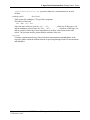
NAME
state
Set initial conditions for primary variables
SYNOPSIS
(state
(<state var. name> <method> <data>)
. . .
(<state var. name> <method> <data>)
)
NOTES
This command must be left out when reading initial data from a restart file using the
restart command.
Examples:
(<state var. name>) (by-key("<elem. range>"<value>)
. . .
("<elem. range>"<value>))
(<state var. name>
by-set <vector>)
where <vector> = [ #<n> <v0> <v1> . . .]
and <n> is number of components (the #<n> field is optional).
Here, [ and ] are actual characters and do not represent delimiters of optional parameters.
(<state var. name> by-xtable <table>),
(<state var. name> by-ytable <table>), or
(<state var. name> by-ztable <table>)
where <table> = (<z0> <val0> <z1> <val1> . . .) is a table of values with respect to
the appropriate x, y, or z coordinate
NOTES:
1. A state variable can appear more than once to overwrite values set by previous
specifications. For example, values for all elements can be set by “by-xtable” or “byset” and then “touched up” using “by-key).”
2. The program will terminate if the primary variables have not been set for each of the
elements.
Reference Manual for the NUFT Flow and Transport Code, Ver. 2.0
UCRL-MA-130651
39
5. Input Data Documentation: Specifying Initial Conditions
NAME
read-restart
Read restart record
SYNOPSIS
(read-restart
(file "<file-name>")
[ (time <restart-time>) ]
)
DESCRIPTION
Sets initial conditions for primary variables by reading in a restart record from a file instead of
using (state . . .)
PARAMETERS
"<file-name>" string
name of the restart file created by the option
(output . . . (restart . . .) . . .)
<restart-time>" real
Time used to search in the restart file;the first restart record with time = <restart-time> will
be read in. The initial time of the simulation run is set by time and overwrites the time
read in through the restart file. If time is not present, the initial of the run is set to the time
read in.
NOTES
Restart filess are created from a previous run using the restart option in the output
command.
Restart Backup
The model will periodically write out restart records so that the model can be restarted in case of
system failure. The model alternately writes out to two restart files named <prefix>.re0 and
<prefix>.re1, where <prefix> is set by output-prefix. Each file contains a single record;
previous records are overwritten. Two files, instead of a single one, are used to prevent losing a
record if the system fails during a write. The user must check the two files to see which is the
most recent. The model writes to a file at periodic intervals, based on the wall-clock time.
(backup <option>)
optional
<option>
word
If set to on, the model will periodically write backup restarts. If set to off, the model will
not do backups. Default is on.
(backup-period <backup-time>)
optional
<backup-time> t-real Wall-clock time period for model to perform backup restarts
Default value is 10m (i.e., 10 minutes).
Reference Manual for the NUFT Flow and Transport Code, Ver. 2.0
UCRL-MA-130651
40
5. Input Data Documentation: Setting Rock Properties
5.6 Setting Rock Properties
NAME
rocktab
Set rock properties
SYNOPSIS
(rocktab
(<rock-type name>
. . .
)
. . .
(<rock-type name>
. . .
)
)
DESCRIPTION
Sets rock properties for each rock type
PARAMETERS
<rock-type name>
the name of the rock type
Reference Manual for the NUFT Flow and Transport Code, Ver. 2.0
UCRL-MA-130651
41
5. Input Data Documentation: Setting Source Terms
5.7 Setting Source Terms
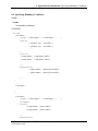
NAME
srctab
Set source terms
SYNOPSIS
(srctab
(compflux <comp-name>
(range "<elem-range>" "<elem-range>" . . .)
(table <flux-table>)
[ (enthalpy <enthalpy-table>) ]
)
. . .
(compflux
. . .
)
(phaseflux <phase>
(name <phaseflux-name>)
(range "<elem-range>" "<elem-range>" . . .)
(table <phase-flux-table>)
(setcomp
(<comp-name>
(table <conc-table>)
following only for thermal models
[ (enthalpy <enthalpy-table>) ]
)
. . .
(<comp-name> internal)
. . .
(<comp-name>
. . .
)
)
)
. . .
(phaseflux
. . .
)
)
Reference Manual for the NUFT Flow and Transport Code, Ver. 2.0
UCRL-MA-130651
42
5. Input Data Documentation: Setting Source Terms
DESCRIPTION
Specifies the component flux into an element or range of elements through a table of source
fluxes at specified points in time.
NOTES
Linear interpolation is used for time intervals between the table values. Positive flux is flux
into an element; negative flux is out of an element.
PARAMETERS
<comp-name>
word
Name of the component (model-specific), which will be forced out or into the element(s)
<elem-range>
pattern string
Range of elements that will have the source term flux specified by the flux table
<flux-table>
table
Component mass flux table of the form
<t0> <q0> <t1> <q1> . . .
where the time values are given by <t0>, <t1>, . . . , which are of data type t-real,
and the mass flux values are <q0>, <q1>, . . ., which are of data type real and are
in units of kg/sec (except that us1p model uses volumetric flux m 3/s). (See Section 6 for
an important note.)
<phase>
Name of the phase
name
<phaseflux-name>
name
Name of the phase flux set
This is used by output options.
<phase-flux-table>
list of reals
Table of mass fluxes of the phase that are of the form
<t0> <q0> <t1> <q1> . . .
where the time values are given by <t0>, <t1>, . . ., which are of data type t-real,
and the mass flux at these times are <q0>, <q1>, . . . , which are of data type real
and are in units of kg/sec. Linear interpolation is used for values between the time values.
The last time must be greater than the end time of the run.
<conc-table>
list of reals
Table of mole or mass fraction concentrations of the components within the phase stream;
the table is of the form
<t0> <x0> <t1> <x1> . . .
where the time values are given by <t0>, <t1>, . . . , which are of data type t-real,
and the concentrations are <x0>, <x1>, . . . , which are of data type real. An
alternative is to specify that the component concentrations used for the flux are those of
element itself; this is done by placing the command (<comp> internal) instead of
(<comp> (table <conc-table>) . . .). Concentrations are in mass fraction if
Reference Manual for the NUFT Flow and Transport Code, Ver. 2.0
UCRL-MA-130651
43
5. Input Data Documentation: Setting Source Terms
(input-mass-fraction on) is present. Otherwise, concentrations are in mole
fraction.
<enthalpy-table>
list of reals
Table of specific enthalpies ("J"/kg) of the component
The table is of the form
<t0> <h0> <t1> <h1> . . .
where the time values are given by <t0>, <t1>, . . ., which are of data type t-real,
and the enthalpies at these times are <h0>, <h1>, . . ., which are of data type real
and have units of Joules/kg. Linear interpolation is used for values between the time
values. The last time must be greater than the end time of the run.
internal
Calculate component and energy fluxes based on concentrations and enthalphies in the
respective phase within the element instead of specifying through a table of concentrations
and enthalpies
Reference Manual for the NUFT Flow and Transport Code, Ver. 2.0
UCRL-MA-130651
44
5. Input Data Documentation: Specifying Boundary Conditions
5.8 Specifying Boundary Conditions
NAME
bctab
Set boundary conditions
SYNOPSIS
(bctab
(<bc-name>
(range "<elem-range>" "<elem-range>" . . .)
(tables
(<primary-var> <var-table>)
(<primary-var> <var-table>)
. . .
)
[ (factor
(<comp-name> <comp-factor-table>)
(<comp-name> <comp-factor-table>)
. . .
) ]
[ (phasefactor
(<phase-name> <phase-factor-table>)
(<phase-name> <phase-factor-table>)
. . .
) ]
)
. . .
(<bc-name>
. . .
)
. . .
(<bc-name>
(range "<elem-range>" "<elem-range>" . . .)
(clamped)
[ (factor
(<comp-name> <factor-table>)
(<comp-name> <factor-table>)
. . .
) ]
[ (phasefactor
Reference Manual for the NUFT Flow and Transport Code, Ver. 2.0
UCRL-MA-130651
45
5. Input Data Documentation: Specifying Boundary Conditions
(<phase-name> <phase-factor-table>)
(<phase-name> <phase-factor-table>)
. . .
) ]
)
)
PARAMETERS
<bc-name>
word
Name of the boundary condition
Each boundary condition has a distinct name used for identification by output options.
"<elem-range>"
pattern string
Range of elements that will have the boundary condition
<primary-var>
word
Name of the primary variable (model-specific) that is being specified by the associated
table
<var-table>
table
Table of primary variable values of form
<t0> <var0> <t1> <var1> . . .
where the time values <t0>, <t1>, . . . are of data type t-real, and the entries
<var0>, <var1>, . . . are the corresponding values of the primary variable that is
being specified. (See Section 6 for an important note.) Primary variable values are
calculated from the table using linear interpolation.
factor
This data unit is optional and is used to modify the component mass fluxes by a factor that
can depend on time and that is set by a table. One use of this option is to turn off a
component flux coming out of or into a boundary element at certain time intervals or at all
times. Note that several different components can be specified, each having its own timedependent factor. Tables for all of the components must be present (the components are
model-specific). Leaving the factor data unit out is equivalent to specifying a
modification factor of 1.0 for all time.
phasefactor
This data unit is optional and is used to modify the phase fluxes by a factor that can
depend on time and that is set by a table.
<comp-name>
word
Name of the component flux that will have its flux modified (model-specific)
<phase-name>
word
Name of the phase that will have its flux modified (model-specific)
<comp-factor-table>
table
Table of modification factors for component fluxes
Reference Manual for the NUFT Flow and Transport Code, Ver. 2.0
UCRL-MA-130651
46
5. Input Data Documentation: Specifying Boundary Conditions
It is of the form,
<t0> <fac0> <t1> <fac1> . . .
where the time values <t0>, <t1>, . . . are of data type t-real, and the entries
<fac0>, <fac1>, . . . are the corresponding modification factors. (See Section 6 for
an important note.) Modification factors are calculated from the table using linear
interpolation.
<phase-factor-table>
table
Table of modification factors multiplying all component fluxes in the corresponding phase
given by <phase-name>; format is analogous to <comp-factor-table>
(clamped)
Keeps the primary variables for these elements, as set in state, fixed in time
NOTES
The data: (factor . . .) is optional; if not present, factors will be unity.
Currently, the model may, in some cases, choose time steps so large that it overshoots sharp
changes in a time table. This may be a serious problem if, for example, one wishes to model a
flux that is turned off suddenly. A solution is to use the forcetimes command in output;
this forces the model to hit specified times; in this case, the times at which the boundary
condition changes suddenly.
The model will abort unless the last time value in table is greater than or equal to the ending
time of the simulation as set by tstop.
Reference Manual for the NUFT Flow and Transport Code, Ver. 2.0
UCRL-MA-130651
47
5. Input Data Documentation: Other Options
5.9 Other Options
NAME
element-prefix-delimiter, element-indices-separator
Set format of element names
SYNOPSIS
[ (element-prefix-delimiter "<prefix-sep>") ]
[ (element-indices-separator "<ind-sep>") ]
DESCRIPTION
Changes the format of element names created by genmsh.
NOTES
The genmsh command names the element according to the general format
<elem-prefix>#<i>:<j>:<k>
where <I>, <j>, <k> denote the i, j, and k indices of the element, and <elem-prefix> is set by
the mat command inside genmsh. These commands allow the user to change the separators
“#” and “:” by the single character in the strings "<prefix-sep>" and "<ind-sep>",
respectively.
Reference Manual for the NUFT Flow and Transport Code, Ver. 2.0
UCRL-MA-130651
48
6. Running Flow and Transport Sequentially
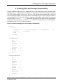
6. Running Flow and Transport Sequentially
In some modules, such as the us1c module, the flow of the fluid phases is first calculated at the
beginning of each step, and then the transport of contaminants is performed using the resulting
flow field. (Other modules, such as usnt, solve for flow and transport simultaneously.) When the
flow and transport models are solved separately, each model has its own set of input data units in
the same input data file. Data units that are common to both models can be placed in a common
data unit called (common . . .), which holds data units used by both the flow and transport
models. If a data unit appears in both the common data unit and the particular unit belonging to
the model, the one in common takes precedence.
General Form for Running Flow and Transport Sequentially
(common
(title . . .)
(outputfile . . .)||{(output-prefix . . .)(output-ext . . .)}
(meshfile . . .)||(genmsh . . .)
(time . . .)
(tstop . . .)
)
(<flow-model-name>
(dt . . .)
(dtmax . . .)
(stepmax . . .)
(state . . .)
(rocktab . . .)
[ (output . . .) ]
[ (srctab . . .) ]
[ (bctab . . .) ]
)
(<transport-model-name>
[
[
[
[
[
)
(dt . . .)
(dtmax . . .)
(stepmax . . .)
(state . . .)
(rocktab . . .)
(output . . .) ]
(srctab . . .) ]
(bctab . . .) ]
(phaseprop . . .) ]
(compprop . . .) ]
Reference Manual for the NUFT Flow and Transport Code, Ver. 2.0
UCRL-MA-130651
49
7. References
7. References
Bear, J., and Y. Bachmat. Introduction to Modeling of Transport Phenomena in Porous Media,
Kluwer Acad. Publishers. 1991.
Behie, A., and P.K. Vinsome. “Block iterative methods for fully implicit reservoir simulation,”
Soc. Petroleum Engineers, paper 9303. 1980.
Edwards, A.L. “TRUMP: a computer program for transient and steady-state temperature
distributions in multidimensional systems.” Springfield, VA: National Tech. Information
Service. 1972.
Grabowski, J.W., P.K. Vinsome, R.C. Lin, A. Behie, and B. Rubin. “A fully implicit, generalpurpose, finite-difference thermal model for in situ combustion and steam,” Soc.
Petroleum Engineers, paper 8396. 1979.
Lee, K., A. Kulshrestha, and J. Nitao. “Interim Report on Verification and Benchmark Testing of
the NUFT Computer Code.” Livermore, CA: Lawrence Livermore National Laboratory.
UCRL-ID-113521. 1993.
Narasimhan, T.N., and P.A. Witherspoon. “An integrated finite difference method for analyzing
fluid flow in porous media,” Water Resour. Res.. 14 255-261. 1978.
Richtmyer, R.D., and K.W. Morto. Difference Methods for Initial-Value Problems. New York,
NY: Interscience Pub. 1967.
Smolarkiewicz, P.K. “A fully multidimensional positive definite advection transport algorithm
with small implicit diffusion,” J. Computational Physics. 54, 325. 1984.
Vinsome, P.K.W. “Orthomin, an iterative method for solving sparse sets of simultaneous linear
equations,” Soc. Petroleum Engineers, paper 5729. 1976.
Reference Manual for the NUFT Flow and Transport Code, Ver. 2.0
UCRL-MA-130651
50
Appendix A. Format of the Mesh File
Appendix A. Format of the Mesh File
The mesh file is free format and can be either of two forms.
First Form
The first form uses element names to specify the connections between two elements:
$elc
% <el-name> <rock-type> <volume> <xc> <yc> <zc>
. . .
% <el-name> <rock-type> <volume> <xc> <yc> <zc>
$end
$con
% <el-name0> <el-name1> <isot> <L0> <L1> <A> <beta>
. . .
% <el-name0> <el-name1> <isot> <L0> <L1> <A> <beta>
$end
Second Form
The second form uses element numbers to specify connections:
$eleme
% <el-num> <el-name> <rock-type> <volume>
...
% <el-num> <el-name> <rock-type> <volume>
$end
$conne
% <mp0> <mp1> <isot> <L0> <L1> <A> <beta>
. . .
% <mp0> <mp1> <isot> <L0> <L1> <A> <beta>
$end
<el-name>
<rock-type>
<volume>
<xc>, <yc>, <zc>
element name (word)
rock type of element (word)
volume of element (real)
coordinates of element centroid
Reference Manual for the NUFT Flow and Transport Code, Ver. 2.0
UCRL-MA-130651
51
Appendix A. Format of the Mesh File
<el-name0>,
<el-name1>
<isot>
<L0>, <L1>
where
<A>
<beta>
<el-num>
<mp0>,
<mp1>
specifies a connection with positive flow going from element <elname0> to <el-name1> (word)
value of 0, 1, or 2 referring to which conductivity K0, K1, or K2 in
(rocktab . . . is used for this connection (integer)
lengths of the parts of the connection that lie in the first and second
elements that define the connection, respectively (real)
flow area of a connection (real)
cosine of the angle of vertical inclination of the connection (real)
the element number starting from 0; must be consecutive (integer) in
$eleme; used primarily for convenience by the user in associating
connections with the elements they connect when the $eleme and
$conne options are used
specifies a flow connection with positive flow going from <mp0> to
<mp1> (integer)
The advantage of the first format is that connections are easily identified by looking at the
element names that they connect, especially if the names are chosen in a convenient manner. The
disadvantage is that more initial set-up time is needed by the model to associate the element
names with the element numbers that will be used during the simulation. For use with more than
4000 elements, the second format is recommended.
Reference Manual for the NUFT Flow and Transport Code, Ver. 2.0
UCRL-MA-130651
52
Appendix B. Numerical Algorithms Used
Appendix B. Numerical Algorithms Used
B.1
Numerical Discretization
NUFT solves balance equations (see, for example, Bear and Bachmat [1991]), which are partial
differential equations whose specific form depends on the particular NUFT module being used.
The balance equations are discretized in space using the integrated, finite-difference method (see
Edwards [1972], Narasimhan and Witherspoon [1978]). Spatial discretization results in a system
of ordinary differential equations of the form
∂u
= f (u, t )
∂t
(1)
where u is the solution vector and f is a vector-valued function.
A first-order, implicit-in-time scheme (Richtmyer and Morton, 1967) is used to discretize the
balance equations for modules with combined flow and contaminant transport. For modules
where flow and transport are solved sequentially, the flow equations are solved using the
implicit-in-time method, and the transport equations can be solved either implicitly or explicitly
in time depending on the user's choice.
When Eq. (1) is solved using the implicit-in-time method, the resulting system of equations that
must be solved at each time step is nonlinear if f is nonlinear.
F(u( n + 1 ) ) ≡ u( n + 1 ) − u( n ) − ∆t ( n ) f(u( n +1) , t ( n +1) ) = 0
(2)
where superscripts represent the time level.
B.2
Newton-Raphson Iteration
The nonlinear system of Eq. (2) is of the form
F(u) = 0
(3)
The Newton-Raphson iterative method is used to solve the equations
J(u n )(u n +1 − u n ) = − F(u n )
(4)
where the matrix
∂F
J(u n ) ≡ i
∂u j
Reference Manual for the NUFT Flow and Transport Code, Ver. 2.0
UCRL-MA-130651
(5)
53
Appendix B. Numerical Algorithms Used
is the Jacobian of the function F evaluated at the n-th iterate, Un. Note that Eq. (4) can be viewed
as a system of linear equations:
Ax = b
(6)
A = J(u n )
(7)
x = un +1 − un
(8)
b = − F(u n )
(9)
where
B.3
Solution of System of Linear Equations
The code currently has two different options for solving the system of linear equations: banded
gaussian elimination and preconditioned conjugate gradient methods.
B.3.1 Banded Gaussian Elimination
First, for convenience, Eq. (4) is rewritten in the matrix form
Ax = b
(10)
[ ]
where A = A i, j is an n × n matrix. It is well known that, in many problems, the matrix A is
banded (i.e., A i, j = 0 for i − j > nb where nb is the matrix half-bandwidth). If nb <<n, it is
advantageous to perform the gaussian elimination only on the elements within the band. This
band becomes more or less filled with non-zero elements as the elimination proceeds.
Problems where A is banded include the case where the problem domain is discretized by a
rectangular mesh and the elements are ordered either rowwise or columnwise.
B.3.2 Orthomin Preconditioned Conjugate Gradient
For the description of the orthomin algorithm and the preconditioning options, see Vinsome
(1976) and Behie et al. (1980).
B.4
Automatic Time-Stepping
The time-stepping algorithm seeks to control the maximum change in the solution vector from
one time step to the next. This control can be accomplished by estimating the time step for the
solution to change by a specified amount based on the solution change that ocurred in the
previous two time steps. During an iteration, if the change in solution from the previous time step
is too large, a re-estimation is performed, and the time step is started over. This method also
controls, to some extent, the time-discretization error.
Reference Manual for the NUFT Flow and Transport Code, Ver. 2.0
UCRL-MA-130651
54
Appendix B. Numerical Algorithms Used
The method is now described in more detail: Let ui be the i-th component of the solution vector
at the current iteration of the Newton-Raphson method, and δui be equal to ui minus the i-th
component of the solution vector at the end of the previous time step. Now, let (δui )max be the
maximum allowed change in the solution. The new reference time step is defined as δt by
δt =
(1 + w )(δui )max
w(δui )max + δui
(11)
Here, w is a “damping” factor (Grabowski et al., 1979) that is chosen between 0 to 1 to prevent
the time step from changing too rapidly. A value of 0.8 is used. The value of δt is adjusted to
stay within 0.5 to 4.0 times the time-step size taken in the previous time step. If the reference
time step is less than the current time step because the solution changed too much, the current
time step is replaced by 0.8 times the reference, and the Newton-Raphson is restarted. The factor
0.8 is there to allow for some margin to prevent an excess of restarts.
If the equations are solved using an explicit-in-time method, the time step is restricted so that the
Courant-Friedrichs-Levy criteria (Richtmyer and Morton, 1967) is satisfied.
Reference Manual for the NUFT Flow and Transport Code, Ver. 2.0
UCRL-MA-130651
55