Download Runstream - Shell Buckling

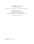
February 19, 2011
BOSOR5 RUN STREAM, STARTING FROM SCRATCH
Commands from the user are in 16 pt bold face. Note: the string,
“bush->”, is not part of the command typed by the user.
The purpose of this run stream is to generate the
valid input file for BOSOR5 called "1.ALL". The
BOSOR5 sample case, 1.ALL, is analogous to the
BIGBOSOR4 sample case also called 1.ALL. Note,
however, that the input data for BOSOR5 are
somewhat different from the input data for BIGBOSOR4.
The valid input file, 1.ALL, is generated mostly by
use of the command, INPUT, by means of which an
interactive session is launched in which the user
generates a number of files, *.SEG1, *.SEG2, ...
in which "*" denotes the user-selected name for
the case, which in this case is "1".
First, go to a working directory where you want to
run BOSOR5. Then do the following:
bush-> bosor5log
BOSOR5 commands have been activated.
Below are the BOSOR5 commands, listed in the order in which you
would probably use them.
input - interactive input of data for each segment
assemble - concatenates the segment data files
bosorread - runs BOSOR5 pre-processor
mainsetup - interactive input of data for main processor
bosormain - runs BOSOR5 main processor
postsetup - interactive input of data for post processor
bosorpost - runs BOSOR5 post processor
bosorplot - generates plot files from most previous run
cleanup - delete all case files except for .DOC file
getsegs - generate segment files from .DOC file
modify - interactively modify a segment or global data file
Please consult the following sources for more information about BOSOR5:
1. .../bosor5/doc/bosor5st.ory (good idea to print this file)
2. Documents listed under HELP5 OVERVIEW DOC
bush-> input
Please enter case name: 1
Do you want to provide data for a new
structural segment, or to add data to
that for an existing structural segment?
(Please answer Y or N) y
Which segment is this?=1
1
Are you correcting, adding to, or checking an existing file?=n
n
BOSOR5 INPUT DATA, INTERACTIVE MODE
Initial prompts are short, and contain data names a new user
will not be familiar with. Please type HELP or H instead of
any datum called for, and you will get more information on that
datum.
Page numbers contained in some of the prompts refer to the
original BOSOR5 user's manual, "BOSOR5--a computer program
for buckling of elastic-plastic complex shells of revolution
including large deflections and creep", Lockheed Missiles &
Space Co. Report LMSC-D407166, December 1974, Vol. 1: User's
manual, input data. This user's manual contains additional
discussion and figures.
NOTE:
This version of BOSOR5 will handle up to 200 shell
segments, rather than the 25 stated as a limit in the
user's manual.
Please provide a title (42 characters or less)...
ALUMINUM FRAME BUCKLING
NSEG = number of shell segments (less than 95)=3
3
The following input must be provided by you for each
shell segment. See p. P1 for a list of the types of
input data required.
NOTE: Up to 200 segments are now permitted in BOSOR5.
NMESH=no. of node points (5=min.;98=max.)=11
11
NTYPEH= control integer (1 or 2 or 3) for nodal point spacing=3
3
Geometry of the current segment...
NSHAPE= indicator (1,2 or 4) for geometry of meridian=1
1
R1
= radius at beginning of segment (see p. P7)=5.218
5.218000
= axial coordinate at beginning of segment=0.
0.000000
R2
= radius at end of segment=5.218
5.218000
Z2
= axial coordinate at end of segment=0.453
0.4530000
Z1
Imperfection geometry....
IMP
= indicator for imperfection (0=none, 1=some)=0
0
NTYPEZ= control (1 or 3) for reference surface location=3
3
ZVAL = distance from leftmost surf. to reference surf.=0
0
Do you want to print out r(s), r'(s), etc. for this segment?=n
n
NRINGS= number (max=20) of discrete rings in this segment=0
0
K=elastic foundation modulus (e.g. lb/in**3)in this seg.=0
0
Do you want general information on loading?=y
y
The following input is related to loading of this
segment. All loads are considered to be axisymmetric
and to be products of spatial times temporal functions.
For example, the pressure, p(s,time), is given by:
p(s,time) = Po(s) * f(time)
in which s is the meridional arc length. In this section
you will be asked to provide only the spatial variation
of the loads [e.g. Po(s) ] and pointers to the temporal
variations, not the temporal variations f(t) themselves.
The f(t) to which the pointers point will be asked for
after data for all the shell segments have been provided
by you. (See pp. P30-P31 for discussion and illustrations.)
There are three types of loading:
1. temperature
2. normal pressure and meridional traction, and
3. line loads and/or imposed displacement components
applied at centroids of discrete rings.
Temperature rise (+) above or fall (-) below that
corresponding to the zero stress state. You will be
asked to provide distributions along the meridian
and through the thickness. (See pp. P32-P39)
NTSTAT = number of temperature callout points along meridian=h
NTSTAT = 0 means no temperature distrib. to be specified;
NTSTAT = 1 means temperature is uniform along meridian;
NTSTAT > 1 means temperature is nonuniform along meridian.
If NTSTAT > 1 you will be asked to provide callout points
(See illustrations on p. P33 and p. P35). BOSOR5 will
automatically linearly interpolate between callout points.
Make sure to include end points of the shell segment in
determining NTSTAT.
NTSTAT = number of temperature callout points along meridian=0
0
Next, provide input for normal pressure and meridional
traction...
NPSTAT = number of meridional callouts for pressure=h
NPSTAT = 0 means no pressure or meridional traction;
NPSTAT = 1 means uniform distributed loading;
NPSTAT > 1 means meridionally nonuniform loading.
In determining NPSTAT, please include the endpoints
of the shell segment. BOSOR5 linearly interpolates
the pressure and meridional traction between callout
points that you will provide along the meridian.
See the illustration at the top of p. P45.
NPSTAT = number of meridional callouts for pressure=2
2
Next provide meridional callout points for pressure...
NTYPE = control for meaning of loading callout (2=z, 3=r)=2
2
Z(I) = axial coordinate of Ith loading callout, z( 1)=0.
0.000000
Z(I) = axial coordinate of Ith loading callout, z( 2)=0.453
0.4530000
Next provide normal pressure and meridional traction
at the meridional callouts...
PN(J)= normal pressure at meridional callout pt. no.( 1)=h
PN is positive as shown in the top figure on p. P45.
Pressure between callouts is calculated by BOSOR5 by
linear interpolation. The actual pressure is a product
P = PN * f(time)
in which the function of time f(time) remains to be
specified.
PN(J)= normal pressure at meridional callout pt. no.( 1)=-1.
-1.000000
PN(J)= normal pressure at meridional callout pt. no.( 2)=-1.
-1.000000
PT(J)= meridional traction at callout point no.( 1)=0
0
PT(J)= meridional traction at callout point no.( 2)=0
0
ISTEP = control integer for time variation of pressure=h
Note that the same time function is to be associated
with both the normal pressure and the meridional
traction.
The control integer, ISTEP, is a pointer which will
cause the appropriate function of time to be associated
with the spatial pressure distribution that you have
just provided. Different functions of time can be
associated with the pressure distributions in
different shell segments. The exact nature of these
time functions will be asked of you later. Right now
all you need do is to specify 1 or 2 or 3, or other
simple integer. Start with an appropriate value which
depends on what other loads you have already specified
in this case up to now. ISTEP should be unity if this
is the first load ever specified in this case.
Each time a new time function is to be introduced, use
a higher integer (higher by 1) than has ever been used
before to specify the time variation of any load, whether
it be for a previously specified temperature distribution,
pressure or surface traction distribution, or line load.
This word 'previous' includes loads that you have
specified in previous segments as well as those specified
previously in the current segment.
ISTEP = control integer for time variation of pressure=1
1
Do you want to print out distributed loads along meridian?=n
n
LINTYP=control for line loads or disp.(0=none,1=some)=h
Line loads must always be associated with a discrete ring,
and they are assumed to act at the discrete ring centroid,
as shown in the Fig. at the bottom of p. P47. Note that
hydrostatic pressure gives rise to line loads, pr/2, at
the ends of the shell structure, thus requiring you to use
LINTYP = 1 for those segments in which pr/2 acts.
Imposed axisymmetric displacement components (USTAR, WSTAR,
CHI, see page P66, left-hand top for positive values) must
always be associated with a discrete ring. In the following
input for loading:
V(K) can mean axial load or axial displacement
(note: positive V (load) [p. P47] is in opposite
direction from positive V (displacement)
[USTAR on p. P66] )
HF(K) can mean radial load or radial displacement
FM(K) can mean meridional moment or meridional rotation
LINTYP=control for line loads or disp.(0=none,1=some)=0
0
Input for orthotropic layered wall construction follows.
Note...circumferential or meridional stiffeners can be
included by smearing their properties as shown on p. P55
and as described below.
Do you
There
Do you
n
LAYERS
want to include smeared stiffeners?=h
is no more help. Do your best.
want to include smeared stiffeners?=n
= number of layers (max. = 6)=h
Be sure to include in LAYERS any layers corresponding
to smeared stringers and/or smeared rings.
Layers are numbered from left-to-right, as shown in the
figure on the bottom of p. P51. "left" and "right" are
based on the assumption that you are facing in the direction
of increasing meridional arc length, s.
LAYERS = number of layers (max. = 6)=1
1
Are all the layers of constant thickness?=h
There is no more help. Do your best.
Are all the layers of constant thickness?=y
y
MATL = type of material for shell wall layer no.( 1)=h
Layers are numbered from left-to-right, as shown in the
figure on the bottom of p. P51. "left" and "right" are
based on the assumption that you are facing in the
direction of increasing meridional arc length, s.
Layers corresponding to parts of smeared stiffeners must
each be associated with a new material index number.
MATL = type of material for shell wall layer no.( 1)=1
1
T(i) = thickness of ith layer (i=1 = leftmost), T( 1)=0.182
0.1820000
G(i) = shear modulus of ith layer, G( 1)=4.051013E+06
4051013.
EX(i)= modulus in meridional direction, EX( 1)=10.8E+06
0.1080000E+08
EY(i)= modulus in circumferential direction, EY( 1)=10.8+06
0.1080000E+08
UXY(i)= Poisson's ratio (EY*UXY = EX*UYX).
UXY( 1)=.333
0.3330000
SM(i)=mass density (e.g. alum.=.00025 lb-sec**2/in**4),SM( 1)=.00025
0.2500000E-03
ALPHA1(i)=coef. thermal exp. in merid. direction, ALPHA1( 1)=0
0
ALPHA2(i)=coef. thermal exp. in circ. direction, ALPHA2( 1)=0
0
EPSALW(i)=maximum allowable eff.strain (percent), EPSALW( 1)=h
There is no more help. Do your best.
EPSALW(i)=maximum allowable eff.strain (percent), EPSALW( 1)=1.6
1.600000
Do you wish to include plasticity in this segment?=h
There is no more help. Do your best.
Do you wish to include plasticity in this segment?=y
y
Do you wish to include creep in this segment?=n
n
Shell wall layer no. 1. A stress-strain curve
the material of this layer must be provided by you
if the same material has not appeared in a previous
layer of this segment or in the shell wall of a
previous shell segment. Note that you must provide
a stress-strain curve here even if the same material
has been specified previously for a discrete ring
segment.
Is this a new shell wall material?=h
There is no more help. Do your best.
Is this a new shell wall material?=y
y
Stress-strain curve for material in shell wall
layer no. 1 . . .
NPOINT = number of points in s.s.curve, layer no.( 1)=h
Please include the stress,strain coordinate (0, 0) in
your determination of a value for NPOINT. NPOINT must
be greater than or equal to 2 and less than 20. If the
material is elastic rather than elastic-plastic, use
NPOINT = 2; use 0. and 1. for the strain coordinates; and
use 0. and E (Young's modulus) for the stress coordinates.
See p. P55 for examples.
NPOINT = number of points in s.s.curve, layer no.( 1)=2
2
NITEG=no. integration pts. thru thickness, layer no.( 1)=h
Use 3 or 5 or 7 or 9 . 5 is usually sufficient unless you are
simulating residual stress patterns due to cold bending. 3 is
good for flanges of stringers or rings that are modelled as a
shell wall layer (smeared out).
NITEG=no. integration pts. thru thickness, layer no.( 1)=h
There is no more help. Do your best.
NITEG=no. integration pts. thru thickness, layer no.( 1)=5
5
Do you want to use power law for stress-strain curve?=h
There is no more help. Do your best.
Do you want to use power law for stress-strain curve?=n
n
EPS(i)=strain coordinates of s-s curve, EPS( 1)=0.
0.000000
EPS(i)=strain coordinates of s-s curve, EPS( 2)=1.
1.000000
SIG(i)=stress coordinates of s-s curve, SIG( 1)=0.
0.000000
SIG(i)=stress coordinates of s-s curve, SIG( 2)=10.8E+06
0.1080000E+08
Do you want to have C(i,j) printed for this segment?=n
n
Want to add more structural segments?y
Which segment is this?=2
2
Are you correcting, adding to, or checking an existing file?=n
n
NMESH=no. of node points (5=min.;98=max.)=10
10
NTYPEH= control integer (1 or 2 or 3) for nodal point spacing=3
3
Geometry of the current segment...
NSHAPE= indicator (1,2 or 4) for geometry of meridian=1
1
R1
= radius at beginning of segment (see p. P7)=5.218
5.218000
Z1
= axial coordinate at beginning of segment=0.2265
0.2265000
R2
= radius at end of segment=4.882
4.882000
Z2
= axial coordinate at end of segment=0.2265
0.2265000
Imperfection geometry....
IMP
= indicator for imperfection (0=none, 1=some)=0
0
NTYPEZ= control (1 or 3) for reference surface location=3
3
ZVAL = distance from leftmost surf. to reference surf.=0.0075
0.7500000E-02
Do you want to print out r(s), r'(s), etc. for this segment?=n
n
NRINGS= number (max=20) of discrete rings in this segment=0
0
K=elastic foundation modulus (e.g. lb/in**3)in this seg.=0
0
Do you want general information on loading?=n
n
Temperature rise (+) above or fall (-) below that
corresponding to the zero stress state. You will be
asked to provide distributions along the meridian
and through the thickness. (See pp. P32-P39)
NTSTAT = number of temperature callout points along meridian=0
0
Next, provide input for normal pressure and meridional
traction...
NPSTAT = number of meridional callouts for pressure=0
0
Next, please provide applied line loads and/or imposed
axisymmetric displacement components for this shell segment...
LINTYP=control for line loads or disp.(0=none,1=some)=0
0
Input for orthotropic layered wall construction follows.
Note...circumferential or meridional stiffeners can be
included by smearing their properties as shown on p. P55
and as described below.
Do you want to include smeared stiffeners?=n
n
LAYERS = number of layers (max. = 6)=1
1
Are all the layers of constant thickness?=y
y
MATL = type of material for shell wall layer no.( 1)=1
1
T(i) = thickness of ith layer (i=1 = leftmost), T( 1)=0.015
0.1500000E-01
G(i) = shear modulus of ith layer, G( 1)=4.051013E+06
4051013.
EX(i)= modulus in meridional direction, EX( 1)=10.8E+06
0.1080000E+08
EY(i)= modulus in circumferential direction, EY( 1)=10.8E+06
0.1080000E+08
UXY(i)= Poisson's ratio (EY*UXY = EX*UYX).
UXY( 1)=.333
0.3330000
SM(i)=mass density (e.g. alum.=.00025 lb-sec**2/in**4),SM( 1)=.00025
0.2500000E-03
ALPHA1(i)=coef. thermal exp. in merid. direction, ALPHA1( 1)=0
0
ALPHA2(i)=coef. thermal exp. in circ. direction, ALPHA2( 1)=0
0
EPSALW(i)=maximum allowable eff.strain (percent), EPSALW( 1)=1.6
1.600000
Do you wish to include plasticity in this segment?=y
y
Do you wish to include creep in this segment?=n
n
Shell wall layer no. 1. A stress-strain curve
the material of this layer must be provided by you
if the same material has not appeared in a previous
layer of this segment or in the shell wall of a
previous shell segment. Note that you must provide
a stress-strain curve here even if the same material
has been specified previously for a discrete ring
segment.
Is this a new shell wall material?=n
n
Do you want to have C(i,j) printed for this segment?=n
n
Want to add more structural segments?y
Which segment is this?=3
3
Are you correcting, adding to, or checking an existing file?=n
n
NMESH=no. of node points (5=min.;98=max.)=7
7
NTYPEH= control integer (1 or 2 or 3) for nodal point spacing=3
3
Geometry of the current segment...
NSHAPE= indicator (1,2 or 4) for geometry of meridian=1
1
R1
= radius at beginning of segment (see p. P7)=4.882
4.882000
Z1
= axial coordinate at beginning of segment=.182
0.1820000
R2
= radius at end of segment=4.882
4.882000
Z2
= axial coordinate at end of segment=.271
0.2710000
Imperfection geometry....
IMP
= indicator for imperfection (0=none, 1=some)=0
0
NTYPEZ= control (1 or 3) for reference surface location=3
3
ZVAL = distance from leftmost surf. to reference surf.=.015
0.1500000E-01
Do you want to print out r(s), r'(s), etc. for this segment?=n
n
NRINGS= number (max=20) of discrete rings in this segment=0
0
K=elastic foundation modulus (e.g. lb/in**3)in this seg.=0
0
Do you want general information on loading?=n
n
Temperature rise (+) above or fall (-) below that
corresponding to the zero stress state. You will be
asked to provide distributions along the meridian
and through the thickness. (See pp. P32-P39)
NTSTAT = number of temperature callout points along meridian=0
0
Next, provide input for normal pressure and meridional
traction...
NPSTAT = number of meridional callouts for pressure=0
0
Next, please provide applied line loads and/or imposed
axisymmetric displacement components for this shell segment...
LINTYP=control for line loads or disp.(0=none,1=some)=0
0
Input for orthotropic layered wall construction follows.
Note...circumferential or meridional stiffeners can be
included by smearing their properties as shown on p. P55
and as described below.
Do you want to include smeared stiffeners?=n
n
LAYERS = number of layers (max. = 6)=1
1
Are all the layers of constant thickness?=y
y
MATL = type of material for shell wall layer no.( 1)=1
1
T(i) = thickness of ith layer (i=1 = leftmost), T( 1)=0.015
0.1500000E-01
G(i) = shear modulus of ith layer, G( 1)=4.051013E+06
4051013.
EX(i)= modulus in meridional direction, EX( 1)=10.8E+06
0.1080000E+08
EY(i)= modulus in circumferential direction, EY( 1)=10.8E+06
0.1080000E+08
UXY(i)= Poisson's ratio (EY*UXY = EX*UYX).
UXY( 1)=.333
0.3330000
SM(i)=mass density (e.g. alum.=.00025 lb-sec**2/in**4),SM( 1)=.00025
0.2500000E-03
ALPHA1(i)=coef. thermal exp. in merid. direction, ALPHA1( 1)=0
0
ALPHA2(i)=coef. thermal exp. in circ. direction, ALPHA2( 1)=0
0
EPSALW(i)=maximum allowable eff.strain (percent), EPSALW( 1)=1.6
1.600000
Do you wish to include plasticity in this segment?=y
y
Do you wish to include creep in this segment?=n
n
Shell wall layer no. 1. A stress-strain curve
the material of this layer must be provided by you
if the same material has not appeared in a previous
layer of this segment or in the shell wall of a
previous shell segment. Note that you must provide
a stress-strain curve here even if the same material
has been specified previously for a discrete ring
segment.
Is this a new shell wall material?=n
n
Do you want to have C(i,j) printed for this segment?=n
n
Want to add more structural segments? n
Have you supplied data for all structural
segments? (Please answer Y or N) y
Next, give global input and input for
constraint conditions. Do you want to
supply these data now (Y or N)?y
How many segments in the structure?=3
3
Are you correcting, adding to, or checking an existing file?=n
n
Next, provide data which pertain to the entire structure,
such as time variation of loads, boundary conditions, and
junction conditions...
Do you want information on time functions for loading?=y
y
Data for time variation of loads is next. In common
cases (no creep, all loads varying proportionally and
generally increasing until bifurcation buckling or
collapse occurs) it is advisable to identify "time"
directly with "load" and time increment with load
increment. Hence, whenever possible, the loading
functions of time should be set equal to the time:
f(time) = time
In this way you will be able to read the load directly
from the output; "TIME" will be the same as "load".
Please refer to pp. P30-P31 for examples.
IUTIME = control for time increment (0 or 1). IUTIME=h
0 means time increment varies during case
1 means time increment is constant during case.
Please see the examples on pp. P30-P31 and pp. P61-P63.
For most cases (except perhaps those involving creep) you
will want to set IUTIME = 1.
IUTIME = control for time increment (0 or 1). IUTIME=1
1
DTIME = time increment=h
See the discussion on pp. P30-P31. If you have a situation
in which all loads are being increased in proportion, then
it is best to set the time increment equal to the increment
of what you feel to be the most important load component of
the case. (e.g. external pressure increment). For example,
if you think a shell will collapse at about 100 psi, then
you might wish to reach 100 psi in 10-psi increments. The
time increment, DTIME, you would then set equal to 10. For
most cases, DTIME doesn't signify a real time increment; TIME
in BOSOR5 is just a convenient parameter to use for provision
of applied loads that vary nonproportionally during a case. In
cases involving creep, TIME is real time, of course.
DTIME = time increment=1.0
1.000000
TMAX = maximum time to be encountered during this case=h
As with DTIME, you associate TMAX with the most important
load component and set it equal to the largest value of that
load component that could possibly be of any interest at
all. Overestimate here. For example, if you think the
shell you are studying might collapse at 100 psi, use TMAX
of about 10000 or 100000.
TMAX = maximum time to be encountered during this case=100000.
100000.0
Next, specify the various time functions associated with
the loads on the structure. These are the fi(time) to which
the pointers, ISTEP, IDTEMP, etc. point.
NFTIME= number of different functions of time=h
For example, you may have a case involving a temperature
distribution which is constant with time and a pressure
distribution which varies linearly with time. In such a
case, NFTIME = 2, since there are two functions of time,
one function (the temperature) a constant and the other
(the pressure) a varying quantity (See example, p. P30).
NFTIME must be equal to the highest value of any of the
pointers, IDTEMP, ISTEP, ISTEP1, ISTEP2, ISTEP3, which
were specified in the sections on temperature and
loading input. (See page P38 for IDTEMP, p. P44 for ISTEP,
p. P46 for ISTEP1, ISTEP2, ISTEP3.)
NFTIME= number of different functions of time=1
1
Next, please provide the time variations of loading which
correspond to the pointers IDTEMP, ISTEP, etc. that you
have already given. Each time-varying load factor is to be
provided by you in the form of a vector of time callouts,
T(i,j), j=1,NPOINT, followed by a vector of corresponding
load factors F(i,j), j=1,NPOINT, where i = 1, 2, 3...NFTIME.
The index j is in the inner loop.
NPOINT=no. of points j for ith load factor F(i,j). i=( 1)=h
NPOINT must be greater than or equal to 2 and less than
or equal to 50. For constant or linearly varying loads
NPOINT should be 2. See p. P63 for an example. In
common cases, the time increase is identified directly
with the load increase: time = load, essentially. In
such a case, NPOINT = 2.
NPOINT=no. of points j for ith load factor F(i,j). i=( 1)=2
2
T(i,j)=jth time callout for ith time function, j =( 1)=h
T(i,j) must be less than or equal to TMAX.
T(i,j)=jth time callout for ith time function, j =( 1)=0.
0.000000
T(i,j)=jth time callout for ith time function, j =( 2)=10000.
10000.00
Next, provide the vector of load factors F(i,j). i=
F(i,j)=jth value for ith load factor. j =( 1)=h
For common cases (no creep) it is advisable to identify
the load factor F(i,j) with time T(i,j). Thus,
F(i,j) = T(i,j) ; in other words, f(time) = time
Then in the output when "time" is printed, you will know
directly what the load is.
F(i,j)=jth value for ith load factor. j =( 1)=0.
0.000000
F(i,j)=jth value for ith load factor. j =( 2)=10000.
10000.00
How many segments are there in the structure?=3
3
Four kinds of constraint conditions exist in BOSOR5:
1.
2.
3.
4.
constraints to ground (e.g. boundary conditions)
juncture compatibility conditions
regularity conditions at poles (where radius r = 0)
constraints to prevent rigid body displacements
See the figs. on p. P67, for example. There is a constraint
to ground (boundary condition) at Seg. 8, Point 8; there are
several juncture conditions (e.g. Seg. 2, Pt. 1 is connected
to Seg. 1, Pt. 9); there are several poles (e.g. Seg. 1,
Pt. 1). Note that if a shell is not anywhere attached to
ground, such as is the case for the example shown on p. P75,
you must choose a node at which to prevent rigid body
motion. You must choose this node in the section below where
you are asked about constraints to ground. In a section
following the "constraints-to-ground" section, you will
be asked to provide specific data for preventing rigid body
motion. Types of rigid body motion are shown on p. P73. An
example of appropriate input data is listed on p. P75, bottom.
CONSTRAINT CONDITIONS FOR SEGMENT NO. ISEG = 1
Number of poles (places where r=0) in SEGMENT=0
0
At how many stations is this segment constrained to ground?=1
1
INODE = nodal point number of constraint to ground, INODE( 1)=1
1
IUSTAR=axial displacement constraint (0 or 1 or 2)=1
1
IVSTAR= circumferential displacement (0=free, 1=constrained)=0
0
IWSTAR=radial displacement(0=free,1=constrained,2=imposed)=0
0
ICHI=meridional rotation (0=free,1=constrained,2=imposed)=0
0
D1
= radial component of offset of ground support=0
0
D2
= axial component of offset of ground support=0
0
Is this constraint the same for both prebuckling and buckling?=y
y
Is this segment joined to any lower-numbered segments?=n
n
CONSTRAINT CONDITIONS FOR SEGMENT NO. ISEG = 2
Number of poles (places where r=0) in SEGMENT=0
0
At how many stations is this segment constrained to ground?=0
0
Is this segment joined to any lower-numbered segments?=y
y
At how may stations is this segment joined to previous segs.?=1
1
INODE = node in current segment (ISEG) of junction, INODE( 1)=1
1
JSEG = segment no. of lowest segment involved in junction=1
1
JNODE = node in lowest segment (JSEG) of junction=6
6
IUSTAR= axial displacement (0=not slaved, 1=slaved)=1
1
IVSTAR= circumferential displacement (0=not slaved, 1=slaved)=1
1
IWSTAR= radial displacement (0=not slaved, 1=slaved)=1
1
ICHI = meridional rotation (0=not slaved, 1=slaved)=1
1
D1
= radial component of juncture gap=0
0
D2
= axial component of juncture gap=0
0
Is this constraint the same for both prebuckling and buckling?=y
y
CONSTRAINT CONDITIONS FOR SEGMENT NO. ISEG = 3
Number of poles (places where r=0) in SEGMENT=0
0
At how many stations is this segment constrained to ground?=0
0
Is this segment joined to any lower-numbered segments?=y
y
At how may stations is this segment joined to previous segs.?=1
1
INODE = node in current segment (ISEG) of junction, INODE( 1)=4
4
JSEG = segment no. of lowest segment involved in junction=2
2
JNODE = node in lowest segment (JSEG) of junction=10
10
IUSTAR= axial displacement (0=not slaved, 1=slaved)=1
1
IVSTAR= circumferential displacement (0=not slaved, 1=slaved)=1
1
IWSTAR= radial displacement (0=not slaved, 1=slaved)=1
1
ICHI = meridional rotation (0=not slaved, 1=slaved)=1
1
D1
= radial component of juncture gap=0
0
D2
= axial component of juncture gap=0
0
Is this constraint the same for both prebuckling and buckling?=y
y
It may be necessary to provide additional constraint to
ground in order to prevent rigid body motion in the
bifurcation buckling phase of the analysis. All possible
types of rigid body motion are shown on p. P73. Rigid body
motion corresponds to n = 0 or n = 1 circumferential waves.
There is no rigid body component for any harmonic with n
greater than or equal to 2. Note that the following question
applies only to the bifurcation buckling phase of the
analysis, not to the axisymmetric prebuckling phase.
Given existing constraints, are rigid body modes possible?=n
n
WPRALL= maximum allowable displacement, WPRALL=h
There is no more help. Do your best.
WPRALL= maximum allowable displacement, WPRALL=0.1
0.1000000
If you have completed input for all structural
segments and for the constraint conditions,
next give the command ASSEMBLE .
--------------- END OF INTERACTIVE "INPUT" SESSION -----------------There now exist in the working directory the following files:
-rw-r--r--rw-r--r--rw-r--r--rw-r--r--
1
1
1
1
bush
bush
bush
bush
bush
bush
bush
bush
4209
2948
2948
4680
Feb
Feb
Feb
Feb
19
19
19
19
09:41
09:47
09:54
10:14
1.SEG1
1.SEG2
1.SEG3
1.SEG4
The command, "ASSEMBLE" (assemble) concatinates these four files.
bush-> assemble
Please enter case name: 1
How many segments in the model (excluding global data)? 3
1.SEG1
assembled into
1.ALL
1.SEG2
assembled into
1.ALL
1.SEG3
assembled into
1.ALL
1.SEG4
assembled into
1.ALL
All segment files have been assembled. Now give the
command BOSORREAD.
-------- END OF "ASSEMBLE" ----------------------There now exist in the working directory the following files:
-rw-r--r--rw-r--r--rw-r--r--rw-r--r--rw-r--r--
1
1
1
1
1
bush
bush
bush
bush
bush
bush 14760 Feb 19 10:23 1.ALL
bush 4209 Feb 19 09:41 1.SEG1
bush 2948 Feb 19 09:47 1.SEG2
bush 2948 Feb 19 09:54 1.SEG3
bush 4680 Feb 19 10:14 1.SEG4
The file, 1.ALL, contains valid input data for the
BOSORREAD processor of BOSOR5.
------ 1.ALL file generated from the above run stream -----ALUMINUM FRAME BUCKLING
3
$ NSEG = number of shell segments (less than 95)
H
$
H
$ SEGMENT NUMBER
1
1
1
1
1
1
1
1
H
$ NODAL POINT DISTRIBUTION FOLLOWS...
11
$ NMESH=no. of node points (5=min.;98=max.)
3
$ NTYPEH= control integer (1 or 2 or 3) for nodal point spacing
H
$ REFERENCE SURFACE GEOMETRY FOLLOWS...
1
$ NSHAPE= indicator (1,2 or 4) for geometry of meridian
5.218000
$ R1
= radius at beginning of segment (see p. P7)
0.000000
$ Z1
= axial coordinate at beginning of segment
5.218000
$ R2
= radius at end of segment
0.4530000
$ Z2
= axial coordinate at end of segment
H
$ IMPERFECTION SHAPE FOLLOWS...
0
$ IMP
= indicator for imperfection (0=none, 1=some)
H
$ REFERENCE SURFACE LOCATION RELATIVE TO WALL
3
$ NTYPEZ= control (1 or 3) for reference surface location
0
$ ZVAL = distance from leftmost surf. to reference surf.
n
$ Do you want to print out r(s), r'(s), etc. for this segment?
H
$ DISCRETE RING INPUT FOLLOWS...
0
$ NRINGS= number (max=20) of discrete rings in this segment
0
$ K=elastic foundation modulus (e.g. lb/in**3)in this seg.
H
$ TEMPERATURE INPUT FOLLOWS...
y
$ Do you want general information on loading?
0
$ NTSTAT = number of temperature callout points along meridian
H
$ PRESSURE INPUT FOLLOWS...
2
$ NPSTAT = number of meridional callouts for pressure
2
$ NTYPE = control for meaning of loading callout (2=z, 3=r)
0.000000
$ Z(I) = axial coordinate of Ith loading callout, z( 1)
0.4530000
$ Z(I) = axial coordinate of Ith loading callout, z( 2)
-1.000000
$ PN(J)= normal pressure at meridional callout pt. no.( 1)
-1.000000
$ PN(J)= normal pressure at meridional callout pt. no.( 2)
0
$ PT(J)= meridional traction at callout point no.( 1)
0
$ PT(J)= meridional traction at callout point no.( 2)
1
$ ISTEP = control integer for time variation of pressure
n
$ Do you want to print out distributed loads along meridian?
H
$ LINE LOAD INPUT FOLLOWS...
0
$ LINTYP=control for line loads or disp.(0=none,1=some)
H
$ SHELL WALL CONSTRUCTION FOLLOWS...
n
$ Do you want to include smeared stiffeners?
1
$ LAYERS = number of layers (max. = 6)
y
$ Are all the layers of constant thickness?
1
$ MATL = type of material for shell wall layer no.( 1)
0.1820000
$ T(i) = thickness of ith layer (i=1 = leftmost), T( 1)
4051013.
$ G(i) = shear modulus of ith layer, G( 1)
0.1080000E+08 $ EX(i)= modulus in meridional direction, EX( 1)
0.1080000E+08 $ EY(i)= modulus in circumferential direction, EY( 1)
0.3330000
$ UXY(i)= Poisson's ratio (EY*UXY = EX*UYX).
UXY( 1)
0.2500000E-03 $ SM(i)=mass density (e.g. alum.=.00025 lb-sec**2/in**4),SM( 1)
0
$ ALPHA1(i)=coef. thermal exp. in merid. direction, ALPHA1( 1)
0
$ ALPHA2(i)=coef. thermal exp. in circ. direction, ALPHA2( 1)
1.600000
$ EPSALW(i)=maximum allowable eff.strain (percent), EPSALW( 1)
y
$ Do you wish to include plasticity in this segment?
n
$ Do you wish to include creep in this segment?
y
$ Is this a new shell wall material?
2
5
n
0.000000
1.000000
0.000000
0.1080000E+08
n
H
H
H
H
10
3
H
1
5.218000
0.2265000
4.882000
0.2265000
H
0
H
3
0.7500000E-02
n
H
0
0
H
n
0
H
0
H
0
H
n
1
y
1
0.1500000E-01
4051013.
0.1080000E+08
0.1080000E+08
0.3330000
0.2500000E-03
0
0
1.600000
y
n
n
n
H
H
H
H
$
$
$
$
$
$
$
$
$
$
$
$
$
$
$
$
$
$
$
$
$
$
$
$
$
$
$
$
$
$
$
$
$
$
$
$
$
$
$
$
$
$
$
$
$
$
$
$
$
$
$
$
$
$
$
$
$
$
NPOINT = number of points in s.s.curve, layer no.( 1)
NITEG=no. integration pts. thru thickness, layer no.( 1)
Do you want to use power law for stress-strain curve?
EPS(i)=strain coordinates of s-s curve, EPS( 1)
EPS(i)=strain coordinates of s-s curve, EPS( 2)
SIG(i)=stress coordinates of s-s curve, SIG( 1)
SIG(i)=stress coordinates of s-s curve, SIG( 2)
Do you want to have C(i,j) printed for this segment?
END OF DATA FOR THIS SEGMENT
SEGMENT NUMBER
2
2
2
2
2
2
2
2
NODAL POINT DISTRIBUTION FOLLOWS...
NMESH=no. of node points (5=min.;98=max.)
NTYPEH= control integer (1 or 2 or 3) for nodal point spacing
REFERENCE SURFACE GEOMETRY FOLLOWS...
NSHAPE= indicator (1,2 or 4) for geometry of meridian
R1
= radius at beginning of segment (see p. P7)
Z1
= axial coordinate at beginning of segment
R2
= radius at end of segment
Z2
= axial coordinate at end of segment
IMPERFECTION SHAPE FOLLOWS...
IMP
= indicator for imperfection (0=none, 1=some)
REFERENCE SURFACE LOCATION RELATIVE TO WALL
NTYPEZ= control (1 or 3) for reference surface location
ZVAL = distance from leftmost surf. to reference surf.
Do you want to print out r(s), r'(s), etc. for this segment?
DISCRETE RING INPUT FOLLOWS...
NRINGS= number (max=20) of discrete rings in this segment
K=elastic foundation modulus (e.g. lb/in**3)in this seg.
TEMPERATURE INPUT FOLLOWS...
Do you want general information on loading?
NTSTAT = number of temperature callout points along meridian
PRESSURE INPUT FOLLOWS...
NPSTAT = number of meridional callouts for pressure
LINE LOAD INPUT FOLLOWS...
LINTYP=control for line loads or disp.(0=none,1=some)
SHELL WALL CONSTRUCTION FOLLOWS...
Do you want to include smeared stiffeners?
LAYERS = number of layers (max. = 6)
Are all the layers of constant thickness?
MATL = type of material for shell wall layer no.( 1)
T(i) = thickness of ith layer (i=1 = leftmost), T( 1)
G(i) = shear modulus of ith layer, G( 1)
EX(i)= modulus in meridional direction, EX( 1)
EY(i)= modulus in circumferential direction, EY( 1)
UXY(i)= Poisson's ratio (EY*UXY = EX*UYX).
UXY( 1)
SM(i)=mass density (e.g. alum.=.00025 lb-sec**2/in**4),SM( 1)
ALPHA1(i)=coef. thermal exp. in merid. direction, ALPHA1( 1)
ALPHA2(i)=coef. thermal exp. in circ. direction, ALPHA2( 1)
EPSALW(i)=maximum allowable eff.strain (percent), EPSALW( 1)
Do you wish to include plasticity in this segment?
Do you wish to include creep in this segment?
Is this a new shell wall material?
Do you want to have C(i,j) printed for this segment?
END OF DATA FOR THIS SEGMENT
SEGMENT NUMBER
3
3
3
3
NODAL POINT DISTRIBUTION FOLLOWS...
3
3
3
3
7
3
H
1
4.882000
0.1820000
4.882000
0.2710000
H
0
H
3
0.1500000E-01
n
H
0
0
H
n
0
H
0
H
0
H
n
1
y
1
0.1500000E-01
4051013.
0.1080000E+08
0.1080000E+08
0.3330000
0.2500000E-03
0
0
1.600000
y
n
n
n
H
H
H
H
y
1
1.000000
100000.0
1
2
0.000000
10000.00
0.000000
10000.00
H
3
$
$
$
$
$
$
$
$
$
$
$
$
$
$
$
$
$
$
$
$
$
$
$
$
$
$
$
$
$
$
$
$
$
$
$
$
$
$
$
$
$
$
$
$
$
$
$
$
$
$
$
$
$
$
$
$
$
$
NMESH=no. of node points (5=min.;98=max.)
NTYPEH= control integer (1 or 2 or 3) for nodal point spacing
REFERENCE SURFACE GEOMETRY FOLLOWS...
NSHAPE= indicator (1,2 or 4) for geometry of meridian
R1
= radius at beginning of segment (see p. P7)
Z1
= axial coordinate at beginning of segment
R2
= radius at end of segment
Z2
= axial coordinate at end of segment
IMPERFECTION SHAPE FOLLOWS...
IMP
= indicator for imperfection (0=none, 1=some)
REFERENCE SURFACE LOCATION RELATIVE TO WALL
NTYPEZ= control (1 or 3) for reference surface location
ZVAL = distance from leftmost surf. to reference surf.
Do you want to print out r(s), r'(s), etc. for this segment?
DISCRETE RING INPUT FOLLOWS...
NRINGS= number (max=20) of discrete rings in this segment
K=elastic foundation modulus (e.g. lb/in**3)in this seg.
TEMPERATURE INPUT FOLLOWS...
Do you want general information on loading?
NTSTAT = number of temperature callout points along meridian
PRESSURE INPUT FOLLOWS...
NPSTAT = number of meridional callouts for pressure
LINE LOAD INPUT FOLLOWS...
LINTYP=control for line loads or disp.(0=none,1=some)
SHELL WALL CONSTRUCTION FOLLOWS...
Do you want to include smeared stiffeners?
LAYERS = number of layers (max. = 6)
Are all the layers of constant thickness?
MATL = type of material for shell wall layer no.( 1)
T(i) = thickness of ith layer (i=1 = leftmost), T( 1)
G(i) = shear modulus of ith layer, G( 1)
EX(i)= modulus in meridional direction, EX( 1)
EY(i)= modulus in circumferential direction, EY( 1)
UXY(i)= Poisson's ratio (EY*UXY = EX*UYX).
UXY( 1)
SM(i)=mass density (e.g. alum.=.00025 lb-sec**2/in**4),SM( 1)
ALPHA1(i)=coef. thermal exp. in merid. direction, ALPHA1( 1)
ALPHA2(i)=coef. thermal exp. in circ. direction, ALPHA2( 1)
EPSALW(i)=maximum allowable eff.strain (percent), EPSALW( 1)
Do you wish to include plasticity in this segment?
Do you wish to include creep in this segment?
Is this a new shell wall material?
Do you want to have C(i,j) printed for this segment?
END OF DATA FOR THIS SEGMENT
GLOBAL DATA BEGINS...
LOADING TIME FUNCTIONS FOLLOW
Do you want information on time functions for loading?
IUTIME = control for time increment (0 or 1). IUTIME
DTIME = time increment
TMAX = maximum time to be encountered during this case
NFTIME= number of different functions of time
NPOINT=no. of points j for ith load factor F(i,j). i=( 1)
T(i,j)=jth time callout for ith time function, j =( 1)
T(i,j)=jth time callout for ith time function, j =( 2)
F(i,j)=jth value for ith load factor. j =( 1)
F(i,j)=jth value for ith load factor. j =( 2)
CONSTRAINT CONDITIONS FOLLOW....
How many segments are there in the structure?
H
H
H
0
H
1
1
1
0
0
0
0
0
y
H
n
H
H
H
0
H
0
H
y
1
1
1
6
1
1
1
1
0
0
y
H
H
H
0
H
0
H
y
1
4
2
10
1
1
1
1
0
0
y
H
n
0.1000000
$
$
$
$
$
$
$
$
$
$
$
$
$
$
$
$
$
$
$
$
$
$
$
$
$
$
$
$
$
$
$
$
$
$
$
$
$
$
$
$
$
$
$
$
$
$
$
$
$
$
$
$
$
$
$
$
$
CONSTRAINT CONDITIONS FOR SEGMENT NO.
1
1
1
1
POLES INPUT FOLLOWS...
Number of poles (places where r=0) in SEGMENT
INPUT FOR CONSTRAINTS TO GROUND FOLLOWS...
At how many stations is this segment constrained to ground?
INODE = nodal point number of constraint to ground, INODE( 1)
IUSTAR=axial displacement constraint (0 or 1 or 2)
IVSTAR= circumferential displacement (0=free, 1=constrained)
IWSTAR=radial displacement(0=free,1=constrained,2=imposed)
ICHI=meridional rotation (0=free,1=constrained,2=imposed)
D1
= radial component of offset of ground support
D2
= axial component of offset of ground support
Is this constraint the same for both prebuckling and buckling?
JUNCTION CONDITION INPUT FOLLOWS...
Is this segment joined to any lower-numbered segments?
CONSTRAINT CONDITIONS FOR SEGMENT NO.
2
2
2
2
POLES INPUT FOLLOWS...
Number of poles (places where r=0) in SEGMENT
INPUT FOR CONSTRAINTS TO GROUND FOLLOWS...
At how many stations is this segment constrained to ground?
JUNCTION CONDITION INPUT FOLLOWS...
Is this segment joined to any lower-numbered segments?
At how may stations is this segment joined to previous segs.?
INODE = node in current segment (ISEG) of junction, INODE( 1)
JSEG = segment no. of lowest segment involved in junction
JNODE = node in lowest segment (JSEG) of junction
IUSTAR= axial displacement (0=not slaved, 1=slaved)
IVSTAR= circumferential displacement (0=not slaved, 1=slaved)
IWSTAR= radial displacement (0=not slaved, 1=slaved)
ICHI = meridional rotation (0=not slaved, 1=slaved)
D1
= radial component of juncture gap
D2
= axial component of juncture gap
Is this constraint the same for both prebuckling and buckling?
CONSTRAINT CONDITIONS FOR SEGMENT NO.
3
3
3
3
POLES INPUT FOLLOWS...
Number of poles (places where r=0) in SEGMENT
INPUT FOR CONSTRAINTS TO GROUND FOLLOWS...
At how many stations is this segment constrained to ground?
JUNCTION CONDITION INPUT FOLLOWS...
Is this segment joined to any lower-numbered segments?
At how may stations is this segment joined to previous segs.?
INODE = node in current segment (ISEG) of junction, INODE( 1)
JSEG = segment no. of lowest segment involved in junction
JNODE = node in lowest segment (JSEG) of junction
IUSTAR= axial displacement (0=not slaved, 1=slaved)
IVSTAR= circumferential displacement (0=not slaved, 1=slaved)
IWSTAR= radial displacement (0=not slaved, 1=slaved)
ICHI = meridional rotation (0=not slaved, 1=slaved)
D1
= radial component of juncture gap
D2
= axial component of juncture gap
Is this constraint the same for both prebuckling and buckling?
RIGID BODY CONSTRAINT INPUT FOLLOWS...
Given existing constraints, are rigid body modes possible?
WPRALL= maximum allowable displacement, WPRALL
--------------------- end of 1.ALL file ------------------------Next, execute BOSORREAD:
bush-> bosorread
Enter case name: 1
B (background) or F (foreground): f
Running BOSOR5: bosorread, case: 1
Executing bosorread
Normal termination: bosorread
Case 1 preprocessor run completed.
Next, give the command "mainsetup"
0.191u 0.087s 0:00.60 45.0%
0+0k 0+0io 2pf+0w
bush-> mainsetup
Please enter case name: 1
Are you correcting, adding to, or checking an existing file?=n
n
INDIC = analysis type indicator (0 or -2 or -3). INDIC=h
0= nonlinear axisymmetric stress (and collapse) analysis;
-2= axisymmetric prebuckling states and stability determinant
are calculated for several load (time) steps. (See p. M3)
-3= stability determinant is calculated for a case in which
prebuckling states have been obtained in a previous run.
See p. M5.
INDIC = analysis type indicator (0 or -2 or -3). INDIC=-2
-2
Type HELP or H for more information on INDIC, N for "no more"=h
INDIC=0 means that nonlinear axisymmetric stress analysis
will be performed for a sequence of time (load) steps
specified by you either in the BOSOR5 preprocessor or in
the following. The results for every time step are saved so
that the case can be restarted at any time step. It is also
possible to restart with a different value of INDIC.
INDIC = -2 means that a nonlinear axisymmetric stress
analysis will be performed and that the stability determinant
will be calculated for several time steps for a certain
fixed number, N0B, of circumferential waves. If the stability
determinant for N0B waves changes sign in the user-specified
time range, then bifurcation buckling loads are calculated
for a range of circumferential wave numbers, NMINB through
NMAXB in increments of INCRB, with NMINB, NMAXB, INCRB to be
provided by you. See the figure at the bottom of p. M3.
(Type H for more help, N for no more.)
Type HELP or H for more information on INDIC, N for "no more"=h
INDIC = -2 (continued) If the stability determinant does
not change sign eigenvalues for the range NMINB to NMAXB are
still computed. In either case (whether or not the
stability determinant changes sign) you should pursue the
buckling analysis in a restart for a new circumferential
wavenumber: that wavenumber corresponding to the minimum
eigenvalue, as shown in Fig (3) at the bottom of p. M3.
INDIC = - 3 means that the stability determinant for a given
number, N0B, of circumferential waves will be calculated for
a sequence of time steps for which the prebuckling analysis
was done in a previous run with INDIC = 0 or INDIC = -2.
Bifurcation buckling loads are calculated for a userprovided range, NMINB to NMAXB, of circumferential wavenumbers
as described above.
(Type H for more information on INDIC, N for no more.)
Type HELP or H for more information on INDIC, N for "no more"=h
Note...In problems involving bifurcation buckling in the
plastic range of material behavior, the actual values of
the eigenvalues obtained by BOSOR5 are not too meaningful.
The sign of the eigenvalues and their relationship to
eachother (that is, for which circumferential wave number
is there a minimum eigenvalue) are important, however.
Briefly, the eigenvalue analysis in BOSOR5 has two purposes:
1. to help the search for a minimum buckling load
with respect to the number of circumferential waves;
2. to yield buckling mode shapes, which guide the
engineer toward a better design.
Type HELP or H for more
There is no more help.
Type HELP or H for more
n
IDEFORM=indicator (0 or
information on INDIC, N for "no more"=h
Do your best.
information on INDIC, N for "no more"=n
1) for type of plasticity theory=h
IDEFORM = 0 means that flow theory will be used to
calculate the constitutive law for both
the prebuckling and the bifurcation buckling
analyses;
IDEFORM = 1 means that flow theory will be used in the
prebuckling analysis and deformation theory
in the bifurcation buckling analysis.
NOTE...In order to run INDIC = -3 with deformation theory you
must have previously run INDIC = -2 with IDEFORM = 1.
IDEFORM=indicator (0 or 1) for type of plasticity theory=0
0
ICPRE = control (0 or 1) for type of eigenvalue problem=h
In cases for which all loads (and temperatures) vary
with pseudo-time in the same proportion, use ICPRE = 1.
Otherwise, use ICPRE = 0. For more details see the
discussion on the right-hand side of p. 407 of the paper
by Lagae and Bushnell, "Elastic-plastic buckling of
torispherical vessel heads", Nuclear Engineering and Design,
Vol. 48 (1978) pp 405-414
ICPRE = control (0 or 1) for type of eigenvalue problem=1
1
Do you want to reverse the rate of loading?=h
For example, you may wish to unload from the latest
converged step or from some earlier step.
Do you want to reverse the rate of loading?=n
n
KSTEP = starting time step number=h
If this is the first run (not a restart) KSTEP must be 0.
If this is a restart, then KSTEP must be equal to a value
for which prebuckling results have already been obtained
in a previous run. (After the first run, KSTEP = 1
corresponds to the first time step.
KSTEP = starting time step number=0
0
KMAX = maximum (less than 49) time step number=h
As a rule of thumb, do less than 10 time steps per run.
Look at your results after each run and make use of the
restart capability.
KMAX = maximum (less than 49) time step number=2
2
MAXTRL = maximum number of trials at each load level=h
The figure on p. M7 explains what is meant by a "trial". In
BOSOR5 several trials for a converged solution are attempted
at each time step (level of loading). The purpose of each
trial is to obtain updated material properties. Use between
3 and 10, usually closer to 3 for best results.
MAXTRL =
maximum number of trials at each load level=5
5
ITMAX = maximum number of Newton iterations for each trial=h
ITMAX between 4 and 10 is recommended. 6 is a good number.
ITMAX = maximum number of Newton iterations for each trial=6
6
ITIME = control (0 or 1) for time increments=h
ITIME = 0 means use time increment(s) specified in
the preprocessor;
ITIME = 1 means use a new time increment
ITIME = control (0 or 1) for time increments=0
0
Do you wish to force the material to remain elastic?=h
Usual answer is N. If you are having numerical difficulty
you may want to answer Y.
Do you wish to force the material to remain elastic?=n
n
N0B
= starting number of circ. waves (buckling analysis)=h
Make N0B your best current estimate of the critical
circumferential wavenumber. See pp. M12 and M13 for
estimates.
N0B
= starting number of circ. waves (buckling analysis)=6
6
NMINB = minimum number of circ. waves (buckling analysis)=5
5
NMAXB = maximum number of circ. waves (buckling analysis)=20
20
INCRB = increment in number of circ. waves (buckling)=1
1
TIME = starting time (need not be zero in initial run)=h
Note... TIME must be less than TMAX (see preprocessor)
TIME = starting time (need not be zero in initial run)=0
0
Do you want stations where plastic flow occurs listed?=y
y
Next, give the command BOSORMAIN
------------------ end of the MAINSETUP interactive session -------------We now have the following files pertaining to the case called "1":
-rw-r--r--rw-r--r--rw-r--r--rw-r--r--rw-r--r--rw-r--r--rw-r--r--rw-r--r--rw-r--r--rw-r--r--
1
1
1
1
1
1
1
1
1
1
bush
bush
bush
bush
bush
bush
bush
bush
bush
bush
bush 14760 Feb 19 10:23 1.ALL
bush 36588 Feb 19 10:29 1.BLK
bush 14749 Feb 19 10:29 1.DOC
bush
1213 Feb 19 10:43 1.IMP
bush
9467 Feb 19 10:29 1.OUT
bush 102912 Feb 19 10:29 1.RAN
bush
4209 Feb 19 09:41 1.SEG1
bush
2948 Feb 19 09:47 1.SEG2
bush
2948 Feb 19 09:54 1.SEG3
bush
4680 Feb 19 10:14 1.SEG4
The interactive "MAINSETUP" input data are saved in the file, 1.IMP,
a list of which follows:
------------ 1.IMP file ----------------------2
$
$
$
$
$
$
$
$
$
$
$
$
$
$
$
$
$
n
0
1
n
0
2
5
6
0
n
6
5
20
1
0
y
INDIC = analysis type indicator (0 or -2 or -3). INDIC
Type HELP or H for more information on INDIC, N for "no more"
IDEFORM=indicator (0 or 1) for type of plasticity theory
ICPRE = control (0 or 1) for type of eigenvalue problem
Do you want to reverse the rate of loading?
KSTEP = starting time step number
KMAX = maximum (less than 49) time step number
MAXTRL = maximum number of trials at each load level
ITMAX = maximum number of Newton iterations for each trial
ITIME = control (0 or 1) for time increments
Do you wish to force the material to remain elastic?
N0B
= starting number of circ. waves (buckling analysis)
NMINB = minimum number of circ. waves (buckling analysis)
NMAXB = maximum number of circ. waves (buckling analysis)
INCRB = increment in number of circ. waves (buckling)
TIME = starting time (need not be zero in initial run)
Do you want stations where plastic flow occurs listed?
------------------- end of 1.IMP file ----------------------
bush-> bosormain
Enter case name: 1
B (background) or F (foreground): f
Running BOSOR5: bosormain, case: 1
Executing bosormain
Normal termination: bosormain
Case 1 mainprocessor run completed.
Next, give the command "mainsetup" or "postsetup"
0.110u 0.077s 0:00.54 33.3%
0+0k 0+0io 2pf+0w
The files in the working directory are now as follows:
-rw-r--r--rw-r--r--rw-r--r--rw-r--r--rw-r--r--rw-r--r--rw-r--r--rw-r--r--rw-r--r--rw-r--r--rw-r--r--
1
1
1
1
1
1
1
1
1
1
1
bush
bush
bush
bush
bush
bush
bush
bush
bush
bush
bush
bush 14760 Feb 19 10:23 1.ALL
bush 36588 Feb 19 10:46 1.BLK
bush 14749 Feb 19 10:29 1.DOC
bush
1213 Feb 19 10:43 1.IMP
bush 12320 Feb 19 10:46 1.MAI
bush 21787 Feb 19 10:46 1.OUT
bush 126464 Feb 19 10:46 1.RAN
bush
4209 Feb 19 09:41 1.SEG1
bush
2948 Feb 19 09:47 1.SEG2
bush
2948 Feb 19 09:54 1.SEG3
bush
4680 Feb 19 10:14 1.SEG4
The file, 1.MAI, contains the output data from the execution
of the BOSOR5 processor, BOSORMAIN. The 1.MAI file is as
follows:
-------------- 1.MAI file (output from BOSORMAIN --------------2
n
0
$ INDIC = analysis type indicator (0 or -2 or -3). INDIC
$ Type HELP or H for more information on INDIC, N for "no more"
$ IDEFORM=indicator (0 or 1) for type of plasticity theory
1
n
0
2
5
6
0
n
6
5
20
1
0
y
$
$
$
$
$
$
$
$
$
$
$
$
$
$
ICPRE = control (0 or 1) for type of eigenvalue problem
Do you want to reverse the rate of loading?
KSTEP = starting time step number
KMAX = maximum (less than 49) time step number
MAXTRL = maximum number of trials at each load level
ITMAX = maximum number of Newton iterations for each trial
ITIME = control (0 or 1) for time increments
Do you wish to force the material to remain elastic?
N0B
= starting number of circ. waves (buckling analysis)
NMINB = minimum number of circ. waves (buckling analysis)
NMAXB = maximum number of circ. waves (buckling analysis)
INCRB = increment in number of circ. waves (buckling)
TIME = starting time (need not be zero in initial run)
Do you want stations where plastic flow occurs listed?
ALUMINUM FRAME BUCKLING
INDIC = analysis type indicator (0 or -2 or -3). INDIC=
-2
Type HELP or H for more information on INDIC, N for "no more"= n
IDEFORM=indicator (0 or 1) for type of plasticity theory=
0
ICPRE = control (0 or 1) for type of eigenvalue problem=
1
Do you want to reverse the rate of loading?= n
KSTEP = starting time step number=
0
KMAX = maximum (less than 49) time step number=
2
MAXTRL = maximum number of trials at each load level=
5
ITMAX = maximum number of Newton iterations for each trial=
6
ITIME = control (0 or 1) for time increments=
0
Do you wish to force the material to remain elastic?= n
N0B
= starting number of circ. waves (buckling analysis)=
6
NMINB = minimum number of circ. waves (buckling analysis)=
5
NMAXB = maximum number of circ. waves (buckling analysis)=
20
INCRB = increment in number of circ. waves (buckling)=
1
INITIAL BUCKLING OR VIBRATION WAVE NO.=
6, MINIMUM WAVE NO.=
5,
MAXIMUM WAVE NO.=
20, INCREMENT=
1
1 EIGENVALUES SOUGHT FOR EACH CIRCUMFERENTIAL WAVE NUMBER.
TIME = starting time (need not be zero in initial run)=
Do you want stations where plastic flow occurs listed?= y
1
***** CALCULATIONS BEGIN FOR TIME STEP NUMBER
TIME =
1
0.00000000E+00 CURRENT TIME INCREMENT =
*****
1.00000000E+00
SEGMENT
PRESSURE MULTIPLIER
TEMPERATURE MULTIPLIER
AMPLITUDES BY DISTRIBUTIONS GIVEN FOR EACH SEGMENT)
0
1
2
3
0.00000000E+00
0.00000000E+00
0.00000000E+00
0
0.00000000E+00
0.00000000E+00
0.00000000E+00
(MULTIPLY THESE
ENTER THE NEWTON-RAPHSON ITERATION LOOP FOR TIME STEP NO.
0.000000E+00
TRIAL NO. 1 ITERATION NO. 1 MAXIMUM DISPLACEMENT =
DISPLACEMENT, ENDUV= 0.0000E+00
TRIAL NO. 1 ITERATION NO. 2 MAXIMUM DISPLACEMENT =
DISPLACEMENT, ENDUV= 0.0000E+00
1
TIME =
0.00000000E+00 END
0.00000000E+00 END
NEWTON-RAPHSON ITERATIONS HAVE CONVERGED.
NEXT CALCULATE THE PREBUCKLING STRAINS AND UPDATE THE MATERIAL
PROPERTIES.
ENTER THE NEWTON-RAPHSON ITERATION LOOP FOR TIME STEP NO.
0.000000E+00
TRIAL NO. 2 ITERATION NO. 1 MAXIMUM DISPLACEMENT =
DISPLACEMENT, ENDUV= 0.0000E+00
1
TIME =
0.00000000E+00 END
NEWTON-RAPHSON ITERATIONS HAVE CONVERGED.
NEXT CALCULATE THE PREBUCKLING STRAINS AND UPDATE THE MATERIAL
PROPERTIES.
ALL INFORMATION HAS BEEN STORED UP TO AND INCLUDING
CURRENT TIME =
0.000E+00
Seg.
1; Max.eff.strain(%)=
1.0000E+17
Seg.
2; Max.eff.strain(%)=
1.0000E+17
Seg.
3; Max.eff.strain(%)=
1.0000E+17
time
TIME
0.000000E+00
0.000000E+00
1.
0.0000E+00 material ok
; strain margin=
0.0000E+00 material ok
; strain margin=
0.0000E+00 material ok
; strain margin=
Maximum prebuckling displacement, WPREMX=
Displacement margin,
WPRMAR=
Maximum
Displacement
WPREMX
0.000000E+00
0.000000E+00
TIME STEP NO.
0.0000E+00
1.0000E+17
time step
KSTEP= 1
End
Displacement
time
time step
ENDUV
TIME
KSTEP= 1
0.000000E+00 0.000000E+00
0.000000E+00 0.000000E+00
End of displacement-time curve for KSTEP=
1
TIME STEP NO. 1 TIME=
0.000E+00
N =
***** STABILITY DETERMINANT = -1.949E+06*10**
TIME STEP
1
NO. OF NEGATIVE ROOTS=
9
NO. OF LAGRANGE MULTIPLIERS=
1
***** CALCULATIONS BEGIN FOR TIME STEP NUMBER
TIME =
6 CIRCUMFERENTIAL WAVES.
470
2
*****
1.00000000E+00 CURRENT TIME INCREMENT =
1.00000000E+00
SEGMENT
PRESSURE MULTIPLIER
TEMPERATURE MULTIPLIER
AMPLITUDES BY DISTRIBUTIONS GIVEN FOR EACH SEGMENT)
0
1
2
3
1.00000000E+00
0.00000000E+00
0.00000000E+00
9
(MULTIPLY THESE
0.00000000E+00
0.00000000E+00
0.00000000E+00
ENTER THE NEWTON-RAPHSON ITERATION LOOP FOR TIME STEP NO.
1.000000E+00
TRIAL NO. 1 ITERATION NO. 1 MAXIMUM DISPLACEMENT =
DISPLACEMENT, ENDUV= 1.2799E-05
TRIAL NO. 1 ITERATION NO. 2 MAXIMUM DISPLACEMENT =
DISPLACEMENT, ENDUV= 1.2799E-05
2
TIME =
1.30416347E-05 END
1.30416356E-05 END
NEWTON-RAPHSON ITERATIONS HAVE CONVERGED.
NEXT CALCULATE THE PREBUCKLING STRAINS AND UPDATE THE MATERIAL
PROPERTIES.
ENTER THE NEWTON-RAPHSON ITERATION LOOP FOR TIME STEP NO.
1.000000E+00
TRIAL NO. 2 ITERATION NO. 1 MAXIMUM DISPLACEMENT =
DISPLACEMENT, ENDUV= 1.2799E-05
2
TIME =
1.30416356E-05 END
NEWTON-RAPHSON ITERATIONS HAVE CONVERGED.
NEXT CALCULATE THE PREBUCKLING STRAINS AND UPDATE THE MATERIAL
PROPERTIES.
ALL INFORMATION HAS BEEN STORED UP TO AND INCLUDING
CURRENT TIME =
1.000E+00
TIME STEP NO.
2.
Seg.
1; Max.eff.strain(%)=
1.0000E+17
Seg.
2; Max.eff.strain(%)=
1.0000E+17
Seg.
3; Max.eff.strain(%)=
1.0000E+17
0.0000E+00 material ok
; strain margin=
0.0000E+00 material ok
; strain margin=
0.0000E+00 material ok
; strain margin=
Maximum prebuckling displacement, WPREMX=
Displacement margin,
WPRMAR=
Maximum
Displacement
WPREMX
0.000000E+00
0.000000E+00
1.304164E-05
time
TIME
0.000000E+00
0.000000E+00
1.000000E+00
1.3042E-05
7.6668E+03
time step
KSTEP= 2
End
Displacement
time
time step
ENDUV
TIME
KSTEP= 2
0.000000E+00 0.000000E+00
0.000000E+00 0.000000E+00
1.279876E-05 1.000000E+00
End of displacement-time curve for KSTEP=
2
TIME STEP NO. 2 TIME=
1.000E+00
N =
***** STABILITY DETERMINANT = -1.948E+06*10**
TIME STEP
2
NO. OF NEGATIVE ROOTS=
0
**********PLEASE
**********PLEASE
**********PLEASE
**********PLEASE
READ
READ
READ
READ
THE
THE
THE
THE
FOLLOWING
FOLLOWING
FOLLOWING
FOLLOWING
9
6 CIRCUMFERENTIAL WAVES.
470
NO. OF LAGRANGE MULTIPLIERS=
IMPORTANT
IMPORTANT
IMPORTANT
IMPORTANT
NOTICE
NOTICE
NOTICE
NOTICE
**********
**********
**********
**********
THE USER HAS CHECKED FOR BIFURCATION BUCKLING LOADS
FOR N =
6 CIRCUMFERENTIAL WAVES. IT HAS BEEN DETERMINED
BY THE ABOVE CALCULATIONS THAT FOR N =
6
THE STABILITY
DETERMINANT DOES NOT CHANGE SIGN IN THE TIME AND LOAD RANGE
SPECIFIED FOR THIS RUN.
HOWEVER, IT MAY HAPPEN THAT THE MINIMUM NONSYMMETRIC BIFURCATION BUCKLING LOAD CORRESPONDS TO A DIFFERENT VALUE OF N THAN
THE PURPOSE OF THE FOLLOWING CALCULATIONS IS TO DETERMINE FOR WHICH N THE CRITICAL LOAD IS SMALLEST. A SEQUENCE OF
EIGENVALUE PROBLEMS.....
(K1(N) + LAMBDA*K2(N))*Q = 0
IS THEREFORE SET UP, WHERE
6
9
K1(N) = STABILITY STIFFNESS MATRIX CORRESPONDING TO A BUCKLING
MODE WITH N CIRC. WAVES FOR THE STRUCTURE AS LOADED AND DEFORMED BY THE LOADS CORRESPONDING TO TIME STEP NO. 1
K2(N) = LOAD-GEOMETRIC MATRIX FOR N CIRC. WAVES CORRESPONDING
TO THE TOTAL LOAD AT STEP NO. 2
LAMBDA = THE EIGENVALUE. DONT CONCERN YOURSELF WITH
THE ABSOLUTE VALUE OF THIS. ONLY THE SIGN OF THE MINIMUM
LAMBDA AND THE RELATIVE VALUES OF LAMBDA FOR VARIOUS N ARE
SIGNIFICANT IF PLASTICITY OCCURS.
Q = THE EIGENVECTOR
(BUCKLING MODE)
1
ITERATIONS HAVE CONVERGED FOR EIGENVALUE NO. 1
EIGENVALUE = 2.45506E+03,
5 CIRCUMFERENTIAL WAVES
ITERATIONS HAVE CONVERGED FOR EIGENVALUE NO. 1
EIGENVALUE = 2.14970E+03,
6 CIRCUMFERENTIAL WAVES
ITERATIONS HAVE CONVERGED FOR EIGENVALUE NO. 1
EIGENVALUE = 1.93669E+03,
7 CIRCUMFERENTIAL WAVES
ITERATIONS HAVE CONVERGED FOR EIGENVALUE NO. 1
EIGENVALUE = 1.79806E+03,
8 CIRCUMFERENTIAL WAVES
ITERATIONS HAVE CONVERGED FOR EIGENVALUE NO. 1
EIGENVALUE = 1.71769E+03,
9 CIRCUMFERENTIAL WAVES
ITERATIONS HAVE CONVERGED FOR EIGENVALUE NO. 1
EIGENVALUE = 1.68283E+03,
10 CIRCUMFERENTIAL WAVES
ITERATIONS HAVE CONVERGED FOR EIGENVALUE NO. 1
EIGENVALUE = 1.68370E+03,
11 CIRCUMFERENTIAL WAVES
ITERATIONS HAVE CONVERGED FOR EIGENVALUE NO. 1
EIGENVALUE = 1.71289E+03,
12 CIRCUMFERENTIAL WAVES
ITERATIONS HAVE CONVERGED FOR EIGENVALUE NO. 1
EIGENVALUE = 1.76469E+03,
13 CIRCUMFERENTIAL WAVES
ITERATIONS HAVE CONVERGED FOR EIGENVALUE NO. 1
EIGENVALUE = 1.83455E+03,
14 CIRCUMFERENTIAL WAVES
ITERATIONS HAVE CONVERGED FOR EIGENVALUE NO. 1
EIGENVALUE = 1.91879E+03,
15 CIRCUMFERENTIAL WAVES
ITERATIONS HAVE CONVERGED FOR EIGENVALUE NO. 1
EIGENVALUE = 2.01424E+03,
16 CIRCUMFERENTIAL WAVES
ITERATIONS HAVE CONVERGED FOR EIGENVALUE NO. 1
EIGENVALUE = 2.11815E+03,
17 CIRCUMFERENTIAL WAVES
ITERATIONS HAVE CONVERGED FOR EIGENVALUE NO. 1
EIGENVALUE = 2.22801E+03,
18 CIRCUMFERENTIAL WAVES
ITERATIONS HAVE CONVERGED FOR EIGENVALUE NO. 1
EIGENVALUE = 2.34147E+03,
19 CIRCUMFERENTIAL WAVES
ITERATIONS HAVE CONVERGED FOR EIGENVALUE NO. 1
EIGENVALUE = 2.45634E+03,
20 CIRCUMFERENTIAL WAVES
1
**************************************************
**************************************************
**************************************************
MINIMUM BUCKLING LOAD CORRESPONDS TO N=
10 CIRCUMFERENTIAL WAVES.
BUCKLING LOAD IS GREATER THAN THAT SPECIFIED IN TIME STEP NUMBER
1
**************************************************
**************************************************
**************************************************
1
***** CALCULATIONS BEGIN FOR TIME STEP NUMBER
TIME =
1
0.00000000E+00 CURRENT TIME INCREMENT =
*****
0.00000000E+00
SEGMENT
PRESSURE MULTIPLIER
TEMPERATURE MULTIPLIER
AMPLITUDES BY DISTRIBUTIONS GIVEN FOR EACH SEGMENT)
0
1
2
3
0.00000000E+00
0.00000000E+00
0.00000000E+00
0.00000000E+00
0.00000000E+00
0.00000000E+00
(MULTIPLY THESE
TIME STEP NO. 1 TIME=
0.000E+00
N =
10 CIRCUMFERENTIAL WAVES.
***** STABILITY DETERMINANT = -2.647E+07*10** 470
TIME STEP
1
NO. OF NEGATIVE ROOTS=
9
NO. OF LAGRANGE MULTIPLIERS=
1
***** CALCULATIONS BEGIN FOR TIME STEP NUMBER
TIME =
2
1.00000000E+00 CURRENT TIME INCREMENT =
*****
1.00000000E+00
SEGMENT
PRESSURE MULTIPLIER
TEMPERATURE MULTIPLIER
AMPLITUDES BY DISTRIBUTIONS GIVEN FOR EACH SEGMENT)
0
1
2
3
1.00000000E+00
0.00000000E+00
0.00000000E+00
9
(MULTIPLY THESE
0.00000000E+00
0.00000000E+00
0.00000000E+00
TIME STEP NO. 2 TIME=
1.000E+00
N =
10 CIRCUMFERENTIAL WAVES.
***** STABILITY DETERMINANT = -2.646E+07*10** 470
TIME STEP
2
NO. OF NEGATIVE ROOTS=
9
NO. OF LAGRANGE MULTIPLIERS=
***** STABILITY DETERMINANT DOES NOT CHANGE SIGN IN
THE TIME INTERVAL UP TO AND INCLUDING TIME STEP NO.
2 FOR
THE RANGE OF CIRCUMFERENTIAL WAVE NUMBERS TESTED IN THIS RUN
----------------------- end of the 1.MAI file ------------------------The following apply:
1. The material response is entirely elastic in this case because
the applied loading is very small.
2. The output of especial significance in the above list is the
following:
ITERATIONS HAVE CONVERGED FOR EIGENVALUE NO. 1
EIGENVALUE = 2.45506E+03,
5 CIRCUMFERENTIAL WAVES
ITERATIONS HAVE CONVERGED FOR EIGENVALUE NO. 1
EIGENVALUE = 2.14970E+03,
6 CIRCUMFERENTIAL WAVES
9
ITERATIONS HAVE CONVERGED FOR EIGENVALUE NO. 1
EIGENVALUE = 1.93669E+03,
7 CIRCUMFERENTIAL WAVES
ITERATIONS HAVE CONVERGED FOR EIGENVALUE NO. 1
EIGENVALUE = 1.79806E+03,
8 CIRCUMFERENTIAL WAVES
ITERATIONS HAVE CONVERGED FOR EIGENVALUE NO. 1
EIGENVALUE = 1.71769E+03,
9 CIRCUMFERENTIAL WAVES
ITERATIONS HAVE CONVERGED FOR EIGENVALUE NO. 1
EIGENVALUE = 1.68283E+03,
10 CIRCUMFERENTIAL WAVES
ITERATIONS HAVE CONVERGED FOR EIGENVALUE NO. 1
EIGENVALUE = 1.68370E+03,
11 CIRCUMFERENTIAL WAVES
ITERATIONS HAVE CONVERGED FOR EIGENVALUE NO. 1
EIGENVALUE = 1.71289E+03,
12 CIRCUMFERENTIAL WAVES
ITERATIONS HAVE CONVERGED FOR EIGENVALUE NO. 1
EIGENVALUE = 1.76469E+03,
13 CIRCUMFERENTIAL WAVES
ITERATIONS HAVE CONVERGED FOR EIGENVALUE NO. 1
EIGENVALUE = 1.83455E+03,
14 CIRCUMFERENTIAL WAVES
ITERATIONS HAVE CONVERGED FOR EIGENVALUE NO. 1
EIGENVALUE = 1.91879E+03,
15 CIRCUMFERENTIAL WAVES
ITERATIONS HAVE CONVERGED FOR EIGENVALUE NO. 1
EIGENVALUE = 2.01424E+03,
16 CIRCUMFERENTIAL WAVES
ITERATIONS HAVE CONVERGED FOR EIGENVALUE NO. 1
EIGENVALUE = 2.11815E+03,
17 CIRCUMFERENTIAL WAVES
ITERATIONS HAVE CONVERGED FOR EIGENVALUE NO. 1
EIGENVALUE = 2.22801E+03,
18 CIRCUMFERENTIAL WAVES
ITERATIONS HAVE CONVERGED FOR EIGENVALUE NO. 1
EIGENVALUE = 2.34147E+03,
19 CIRCUMFERENTIAL WAVES
ITERATIONS HAVE CONVERGED FOR EIGENVALUE NO. 1
EIGENVALUE = 2.45634E+03,
20 CIRCUMFERENTIAL WAVES
**************************************************
**************************************************
**************************************************
MINIMUM BUCKLING LOAD CORRESPONDS TO N=
10 CIRCUMFERENTIAL WAVES.
BUCKLING LOAD IS GREATER THAN THAT SPECIFIED IN TIME STEP NUMBER
1
**************************************************
**************************************************
**************************************************
Compare the BOSOR5 prediction:
ITERATIONS HAVE CONVERGED FOR EIGENVALUE NO. 1
EIGENVALUE = 1.68283E+03,
10 CIRCUMFERENTIAL WAVES
with that from BIGBOSOR4 listed as follows in the file,
../bigbosor4/case/bigbosor4.runstream:
***** EIGENVALUES AND MODE SHAPES *****
EIGENVALUE(CIRC. WAVES)
=======================================
4.1833E+02(
2)
1.9615E+03(
4)
2.1497E+03(
6)
1.7981E+03(
8)
1.6828E+03(
10) <-- local minimum from BIGBOSOR4.
1.7129E+03(
12)
1.8346E+03(
14)
2.0142E+03(
16)
2.2280E+03(
18)
2.4563E+03(
20)
=======================================
3. In specifying the range of circumferential numbers to be covered
in the bifurcation buckling analysis, we deliberately excluded values
near N = 2 crcumferential waves. Therefore, we are capturing only one
of the 2 minima contained in the "complete" range of N just listed
from the BIGBOSOR4 runstream.
----------------------------------------------------------------Next, we wish to run the BOSOR5 post-processors, POSTSETUP and
BOSORPOST. First, we conduct the interactive session, POSTSETUP.
bush-> postsetup
Please enter case name: 1
Are you correcting, adding to, or checking an existing file?=n
n
Interactive input for BOSOR5 postprocessor...
IPRINT = control (1 or 2 or 3) for list output=h
IPRINT = 1 means prebuckling states listed for selected
time steps;
IPRINT = 2 means buckling modes printed for selected
circumferential wave numbers;
IPRINT = 3 means both prebuckling states and buckling modes
printed for selected time steps and selected
circumferential wave numbers.
IPRINT = control (1 or 2 or 3) for list output=2
2
IPLOT = control (0 or 1 or 2 or 3) for plot output=h
IPLOT
IPLOT
IPLOT
IPLOT
= 0 means no plots at all;
= 1 means prebuckling states plotted for selected
time steps;
= 2 means buckling modes plotted for selected
circumferential wave numbers;
= 3 means prebuckling states and buckling modes
plotted for selected time steps and selected
circumferential wave numbers.
IPLOT
= control (0 or 1 or 2 or 3) for plot output=2
2
NLAST = plot options (-1=none, 0=geometry, 1=u,v,w)=h
NLAST = -1 means no plotting;
0 means plots of undeformed and deformed
geometry only;
1 means plots of geometry and u,v,w vs arc length.
NLAST = plot options (-1=none, 0=geometry, 1=u,v,w)=0
0
Do you want to plot the discretized model?=y
y
Your structure may contain segments that are very short
compared to the whole model being analyzed here. This detail
will not show up well in plots of the entire undeformed and
deformed structure. Therefore you may wish to get expanded
plots of these regions. Please identify these regions by
segment number and give a magnification factor for each region.
Note that the magnification factor must be an integer.
The center of the expanded plot will be at the first point of
the segment so identified. The extent of structure plotted
will of course depend on the magnification factor you choose.
Are there any regions for which you want expanded plots?=n
n
Selection of buckling modes follows...
NMODES=quantity of buckling modes to be listed, plotted=h
One mode/circumferential wave number. You rarely need to
see all of the modes calculated by the main processor; the
critical mode is the most important, of course.
NMODES=quantity of buckling modes to be listed, plotted=1
1
NTHMOD(i)=ith mode calculated in last main run. i=( 1)=h
Use the order in which the modes were calculated in the
last run of the BOSOR5 main processor as a guide here,
not the number of circumferential waves. For example, if
modes for circ. waves n = 5, 10, 15, 20 were calculated in
that order, and you want to list and/or plot the modes
corresponding to n = 5 and n = 15, then set NTHMOD(1) = 1
(first mode calculated) and NTHMOD(2) = 3 (third mode
calculated).
NTHMOD(i)=ith mode calculated in last main run. i=( 1)=6
6
NWAVE(i)=no. of circ. waves in the ith mode. i=( 1)=h
In the above example NWAVE(1) = 5 and NWAVE(2) = 15.
NWAVE(i)=no. of circ. waves in the ith mode. i=( 1)=10
10
Do you want buckling modal output for all the segments?=y
y
Next, give the command BOSORPOST
----------- end of the interactive "POSTSETUP" session -------------------The files now existing in the working directory are as follows:
-rw-r--r--rw-r--r--rw-r--r--rw-r--r--rw-r--r--rw-r--r--rw-r--r--rw-r--r--rw-r--r--rw-r--r--rw-r--r--rw-r--r--
1
1
1
1
1
1
1
1
1
1
1
1
bush
bush
bush
bush
bush
bush
bush
bush
bush
bush
bush
bush
bush 14760 Feb 19 10:23 1.ALL
bush 36588 Feb 19 10:46 1.BLK
bush 14749 Feb 19 10:29 1.DOC
bush
1213 Feb 19 10:43 1.IMP
bush
633 Feb 19 11:08 1.IPP
bush 12320 Feb 19 10:46 1.MAI
bush 21787 Feb 19 10:46 1.OUT
bush 126464 Feb 19 10:46 1.RAN
bush
4209 Feb 19 09:41 1.SEG1
bush
2948 Feb 19 09:47 1.SEG2
bush
2948 Feb 19 09:54 1.SEG3
bush
4680 Feb 19 10:14 1.SEG4
The new file, 1.IPP, contains the input data for POSTSETUP:
------------- the 1.IPP file --------------------2
$ IPRINT = control (1 or 2 or 3) for list output
2
$ IPLOT = control (0 or 1 or 2 or 3) for plot output
0
$ NLAST = plot options (-1=none, 0=geometry, 1=u,v,w)
y
$ Do you want to plot the discretized model?
n
$ Are there any regions for which you want expanded plots?
1
$ NMODES=quantity of buckling modes to be listed, plotted
6
$ NTHMOD(i)=ith mode calculated in last main run. i=( 1)
6
$ NWAVE(i)=no. of circ. waves in the ith mode. i=( 1)
y
$ Do you want buckling modal output for all the segments?
------------- end of the 1.IPP file -----------------
bush-> bosorpost
Enter case name: 1
B (background) or F (foreground): f
Running BOSOR5: bosorpost, case: 1
Executing bosorpost
Normal termination: bosorpost
Case 1 postprocessor run completed.
Next, choose from the commands:
BOSORPLOT, MAINSETUP, POSTSETUP, INPUT, CLEANUP, GETSEGS, OR MODIFY
0.056u 0.076s 0:00.28 42.8%
0+0k 0+0io 1pf+0w
The files now existing in the working directory are as follows:
-rw-r--r--rw-r--r--rw-r--r--rw-r--r--rw-r--r--rw-r--r--rw-r--r--rw-r--r--rw-r--r--rw-r--r--rw-r--r--rw-r--r--rw-r--r--rw-r--r--rw-r--r--
1
1
1
1
1
1
1
1
1
1
1
1
1
1
1
bush
bush
bush
bush
bush
bush
bush
bush
bush
bush
bush
bush
bush
bush
bush
bush 14760 Feb 19 10:23 1.ALL
bush 36588 Feb 19 10:46 1.BLK
bush 14749 Feb 19 10:29 1.DOC
bush
1213 Feb 19 10:43 1.IMP
bush
633 Feb 19 11:08 1.IPP
bush
45 Feb 19 11:10 1.LAB
bush 12320 Feb 19 10:46 1.MAI
bush 26833 Feb 19 11:10 1.OUT
bush
2902 Feb 19 11:10 1.PLT2
bush
5046 Feb 19 11:10 1.POS
bush 126976 Feb 19 11:10 1.RAN
bush
4209 Feb 19 09:41 1.SEG1
bush
2948 Feb 19 09:47 1.SEG2
bush
2948 Feb 19 09:54 1.SEG3
bush
4680 Feb 19 10:14 1.SEG4
The output from the BOSOR5 post-processor, BOSORPOST, is contained
in the 1.POS file, which will not be listed here.
Next, get a plot of the buckling mode chosen during the POSTSETUP
interactive session:
bush-> bosorplot
Please enter the BOSOR5 case name: 1
Do you want to use Xgraph or create a PostScript file? (Choose X or P) p
One moment please...
Text file(s) have been created containing plot data. The names of the
files explain to a greater or lesser extent what the data represent.
Some plot files contain data for more than one plot.
1)
1..R,Z_EIGENMODE_1--N_10
CR)
to QUIT
Please choose the number of the file you wish to plot:1
Plotting: Undeformed & Deformed Axial Station as a function of Radius
The PostScript file, metafile.ps, has been created.
Please choose one of the three options below:
1) Rename the PostScript file this is useful if
you don't have access to a PostScript printer on your
machine, but you wish to save to a file so you can later
transfer it to a different machine for printing.
Example:
mv metafile.ps plot1.ps
2) Enter an "lpr" command. This is useful if your default
printer is not PostScript, but there is a PostScript
printer available on your system.
Example:
lpr -PApplelaser metafile.ps
3) Press the return key.
This executes the command:
lpr metafile.ps
This assumes that your default printer is a PostScript
printer.
Enter your command> <enter>
Printing PostScript plot on the default printer...
Text file(s) have been created containing plot data. The names of the
files explain to a greater or lesser extent what the data represent.
Some plot files contain data for more than one plot.
1)
1..R,Z_EIGENMODE_1--N_10
CR)
to QUIT
Please choose the number of the file you wish to plot: <enter>
The files now existing in the working directory are as follows:
-rw-r--r--
1 bush bush
14760 Feb 19 10:23 1.ALL
-rw-r--r--rw-r--r--rw-r--r--rw-r--r--rw-r--r--rw-r--r--rw-r--r--rw-r--r--rw-r--r--rw-r--r--rw-r--r--rw-r--r--rw-r--r--rw-r--r--rw-r--r--
1
1
1
1
1
1
1
1
1
1
1
1
1
1
1
bush
bush
bush
bush
bush
bush
bush
bush
bush
bush
bush
bush
bush
bush
bush
bush 36588 Feb 19 10:46 1.BLK
bush 14749 Feb 19 10:29 1.DOC
bush
1213 Feb 19 10:43 1.IMP
bush
633 Feb 19 11:08 1.IPP
bush
45 Feb 19 11:10 1.LAB
bush 12320 Feb 19 10:46 1.MAI
bush 26833 Feb 19 11:10 1.OUT
bush
2902 Feb 19 11:10 1.PLT2
bush
5046 Feb 19 11:10 1.POS
bush 126976 Feb 19 11:10 1.RAN
bush
4209 Feb 19 09:41 1.SEG1
bush
2948 Feb 19 09:47 1.SEG2
bush
2948 Feb 19 09:54 1.SEG3
bush
4680 Feb 19 10:14 1.SEG4
bush 13908 Feb 19 11:16 metafile.ps
The plot is contained in the Postscript file, metafile.ps .
cp metafile.ps plot.n10.ps
gv plot.n10.ps
The plot, plot.n10.ps, is shown below.
plot.n10.ps = 1.buckle.n10.png = buckling mode (eigenvector) for N = 10
circumferential waves. The eigenvalue (buckling load factor) as listed
above is: EIGENVALUE = 1.68283E+03,
10 CIRCUMFERENTIAL WAVES
cleanup
-------------------- end of BOSOR5 run stream ---------------