Download User Manuel - Les pages Web d`Aristote

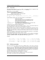
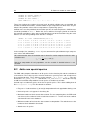
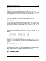
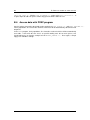
Meudon PDR code
Quick introduction
Franck Le petit & Jacques Le Bourlot
Spring 2014
2
3
Contents
1 Overview
5
2 Installation
7
3 Input and output files
3.1 Input files . . . . . . . . . . . . . . . . . . . . . . . . . . . . . . . . . . . . . . . .
3.2 Output files . . . . . . . . . . . . . . . . . . . . . . . . . . . . . . . . . . . . . . .
9
9
9
4 Parameters of the PDR code
4.1 Geometry & Incident radiation field . . . . . . . . . . . .
4.2 Equation of state : temperature and density profiles . .
4.3 Number of global iterations . . . . . . . . . . . . . . . .
4.4 Photo-reactions & UV radiative transfer . . . . . . . . .
4.5 Cosmic rays ionization rate and secondary photons flux
4.6 Grains properties and physics . . . . . . . . . . . . . . .
4.7 H2 formation and excitation . . . . . . . . . . . . . . . .
4.8 Elementary abundances and metallicity . . . . . . . . .
4.9 Chemistry . . . . . . . . . . . . . . . . . . . . . . . . . .
4.10 Lines intensities and levels excitation . . . . . . . . . . .
5 Analyze results
5.1 Result files . . . . . . . . . . . . . .
5.2 Cloud structure . . . . . . . . . . . .
5.3 Lines intensities and properties . . .
5.4 Spherical clouds . . . . . . . . . . .
5.5 Chemistry analysis . . . . . . . . . .
5.6 Extract radiation field energy density
.
.
.
.
.
.
.
.
.
.
.
.
.
.
.
.
.
.
.
.
.
.
.
.
.
.
.
.
.
.
.
.
.
.
.
.
.
.
.
.
.
.
.
.
.
.
.
.
.
.
.
.
.
.
.
.
.
.
.
.
.
.
.
.
.
.
.
.
.
.
.
.
.
.
.
.
.
.
.
.
.
.
.
.
.
.
.
.
.
.
.
.
.
.
.
.
.
.
.
.
.
.
.
.
.
.
.
.
.
.
.
.
.
.
.
.
.
.
.
.
.
.
.
.
.
.
.
.
.
.
.
.
.
.
.
.
.
.
.
.
.
.
.
.
.
.
.
.
.
.
.
.
.
.
.
.
.
.
.
.
.
.
.
.
.
.
.
.
.
.
.
.
.
.
.
.
.
.
.
.
.
.
.
.
.
.
.
.
.
.
.
.
.
.
.
.
.
.
.
.
.
.
.
.
.
.
.
.
.
.
.
.
.
.
.
.
.
.
.
.
.
.
.
.
.
.
.
.
.
.
.
.
.
.
.
.
.
.
.
.
.
.
.
.
.
.
.
.
.
.
.
.
.
.
.
.
.
.
.
.
.
.
.
.
.
.
.
.
.
.
.
.
.
.
.
.
.
.
.
.
.
.
.
.
11
11
16
17
17
19
19
21
22
22
22
.
.
.
.
.
.
25
25
26
27
28
30
31
A Chemistry file
33
B Add excitation of new species
B.1 Atomic and molecular data files .
B.2 Add a new special species . . .
B.3 Use collision rates . . . . . . . .
B.4 Excitation at formation . . . . . .
B.5 Temporary arrays . . . . . . . . .
B.6 Access data with PREP program
35
35
38
39
39
39
40
.
.
.
.
.
.
.
.
.
.
.
.
.
.
.
.
.
.
.
.
.
.
.
.
.
.
.
.
.
.
.
.
.
.
.
.
.
.
.
.
.
.
.
.
.
.
.
.
.
.
.
.
.
.
.
.
.
.
.
.
.
.
.
.
.
.
.
.
.
.
.
.
.
.
.
.
.
.
.
.
.
.
.
.
.
.
.
.
.
.
.
.
.
.
.
.
.
.
.
.
.
.
.
.
.
.
.
.
.
.
.
.
.
.
.
.
.
.
.
.
.
.
.
.
.
.
.
.
.
.
.
.
.
.
.
.
.
.
.
.
.
.
.
.
.
.
.
.
.
.
.
.
.
.
.
.
.
.
.
.
.
.
4
CONTENTS
5
Chapter 1
Overview
This note is a quick guide explaining how to use the PDR code. It does not describe the
detailed physics in the code. This is done in several articles. References are provided
below.
This is "work in progress": many items are still empty.
It is written for the full fetched PDR code. All options do not exist in the trimmed version
“PDR light”.
The Meudon PDR code simulates a stationary plane-parallel slab of gas and dust illuminated
by an external radiation field coming from one or both sides of the slab (the two intensities can
be different).
At each position in the cloud, the code solves :
• the continuum radiative transfer from the UV to radio wavelengths, taking into account
absorption in the continuum by dust and gas and in discrete transitions of H, H2 and
(optionally) CO and its isotopes. Depending on the algorithm selected to treat these
processes, the code can take into account mutual shielding effects to compute accurately
photo-ionization and photo-dissociation rates.
• the thermal balance. This is done assuming heating rate equals cooling rate. Heating
mechanisms include the photoelectric effect on grains, cosmic rays ionizations, exothermal chemical reactions. Main cooling processes rely on infrared to sub-millimeter line
emission. To solve this the PDR code determines levels excitation of the most important
species taking into account collisional and radiative processes. This includes pumping by
6
1. OVERVIEW
dust I.R. emission as well as atomic / molecular emissions. Photons escape probabilities
are computed taking into account non local effects. Some mechanisms can heat or cool
the gas depending on the local physical conditions, mostly H2 cascades and gas-grains
collisions.
• the chemistry. The chemical network takes into account several hundred species and
thousands reactions. The number of species and reactions can easily be modified. In
version 1.4.4, 1.5.2 and “PDR light” surface reactions with Langmuir-Hinshelwood and
Eley-Rideal mechanisms are implemented for H2 formation.
After a (batch) run, the code produces several output files that contain the structure of the
cloud. Post-processing with PREP program or PDRAnalyser can :
• extract profiles such as abundances, levels populations, temperature of the gas or grains,
heating and cooling rates by individual process, ...
• compute line intensities for different observation angles
• produce an excitation diagram
• compute column densities
• wrap the plan-parallel results on a spherical geometry
• analyze locally the chemical processes
The PDR code can be used for many problems1 . For interpretation of observations, its main
limits are the stationary hypotheses and the plane-parallel geometry. Post-processing permits
to wrap results on 1D spherical models but assumes that the incident radiation field is uniform
around the sphere. So it not possible to model a spherical cloud close to a star (which is a 2D
problem!). The PDR code can also be used as a theoretical tool to study the effects of various
physical and chemical processes in the interstellar medium.
Several articles describe the physics in the PDR code :
• Le Petit et al., ApJ, 2006
• Goicoechea and Le Bourlot, A\&A, 2007
• Gonzalez-Garcia at al., A&A, 2008
• Le Petit et al., A&A, 2009
• Le Bourlot et al., A&A, 2011
Main presentation of the PDR code
UV radiative transfer
Radiative transfer taking into account
non local effects
Moment equations applied to H2 and HD
formation on grains
H2 formation on grains by
Langmuir-Hinshelwood and Eley-Rideal
mechanisms
1 Up to now it has been mainly used to study the physics and chemistry of interstellar clouds. For some other
specific conditions, the user may have to modify some parameters in the source code
7
Chapter 2
Installation
To install the PDR code, you need :
• A fortran 90 compiler
• LAPACK and BLAS libraries
We suggest using gfortran, which is available on all platform and is now fully optimized.
PDR is able to take advantage of its autoparallelization features. Good version for Mac OS can
be found at:
http://hpc.sourceforge.net
Once the code is downloaded, edit the Makefile in the src directory to adapt the call to LAPACK and BLAS libraries1 . Select a compiler and its options, and modify compilation options
to your needs2 . Then run make. This will produce three executables :
• PDR : the PDR code
• PREP : the post-processor code
• CHEM_ANALYSER : the “Chemistry analyser” post-processor
Other tools are provided as a version of DustEM. This code can be used synchronously
with the PDR code to compute more precisely grains properties (temperature, emissivities,
...) than with the PDR code alone. It has to be compiled separately. Before doing so, edit
DM_constants.f90 and modify PATH_TO_PDR to the proper path on your computer. A detailed user guide is not yet available.
In src or src/OTHER_PROG several small programs are provided :
• PREP_PFL : A tool to extract a “profile” file (see Sect 4.2.1) from the output of a run
• read_rf : A tool to read binary radiation files (*.rf) produced by the PDR code
• build_FractalGrid : A tool devoted to the creation of fractal density profiles.
1 On many platform, it is sufficient to specify LIBS1 = -llapack -lblas, since this libraries are standard development tools.
2 You may need first to remove the most agressive optimization option to get a running code. Start with only
-O2.Once the code run smoothly, add more optimization options. This results in a huge gain in running time. You may
need to refer to your compiler user manual or the web.
8
2. I NSTALLATION
9
Chapter 3
Input and output files
3.1
Input files
Input parameters to control a run are provided in several files located in the data directory.
The two most important ones are the pxdr6.in file and a chemistry file identified by the
extension “.chi”. Other files can be modified for specific reasons as to introduce a specific
density-temperature profile or to define a user spectral profile.
Input parameters files are presented in table 3.1.
File
pxdr6.in
*.chi
spectre.flag
*.pfl
photodest.flag
F_*.txt
star.dat
line_of_sight.dat
Description
Input parameters file to control properties of the
cloud
Chemistry file. Provides the list of species, the
elementary abundances, the chemical reactions
File providing the list of species for which detailed
balance is computed (and lines intensities)
Optional specific temperature and density
profiles
List of species for which photo-reaction rates are
computed by direct integration of cross-sections
Optional file providing a specific stellar spectrum
illuminating the cloud
Spectral types used by the code to produce black
bodies illuminating the cloud
Dust extinction coefficients for specific lines of
sight
Page
Table 3.1: List of input files
3.2
Output files
Several output files are produced by the PDR code. They share a common name – set in
pxdr6.in – followed by a specific extension (see table 3.2). The most important file is the
.bin file, which contains the results of the model1 . Other files contains various log or some
1 An iteration number is usually appended to the bin extension (e.g. .bin15). Thus convergence is checked by
comparing the results of the last two iterations, or specific numerical problems can be analyzed by following a variable
from iteration to iteration. During normal usage of the code, only the last file need be kept.
10
3. I NPUT AND OUTPUT FILES
specific radiative quantities.
.bin files are read with the post-processing program PREP. This must be done from the src
directory where PDR was run and with PREP compiled with the same compiler2 .
File
.def
.bin
.uv
.rf
.flin
.Iesc
Description
Log file
Results of a model. Binary file to be read by the post-processing
program PREP
Total attenuation through the cloud
−1
Full map of the energy density uλ (erg cm−3 Å ) as a function of
position AV and wavelength λ (Å). Binary file to be read with the
program read_rf
Incident radiation field
−1
Specific intensity Iλ at cloud edge (erg cm−2 s−1 ster−1 Å )
Page
Table 3.2: List of output files
2 Development are under way to use a much more flexible file format within the framework of the Virtual Observatory.
However, this will not be addressed in this document.
11
Chapter 4
Parameters of the PDR code
Most of the input parameters defining the properties of the cloud computed have to be provided
in the pxdr6.in file located in the data directory. Some other files may have to be modified
as explained below.
The Meudon PDR code is not difficult to use. It is far more difficult to understand the results
because of the non-linearity and coupling of the various physical processes. A good way to
begin to use the code is to run the code with the default pxdr6.in and to play with the results.
It is a low excitation cloud so the physical and chemical processes that can take place are more
limited than in a dense and bright PDR. Once ready to run a real model, the user should ask
to himself :
• which geometry to choose? A 1 side or 2 sides model and with which size?
In most "real" cases, 2 sides models are a good choice. Even to study a bright PDR, it is
better to simulate 2 sides clouds with a large enough size, using a strong radiation field
on one side and the standard ISRF on the other.
• what kind of incident radiation field to use?
The question is important for the study of PDRs. It is common to read in the literature
that the intensity of the radiation field is χ times the ISRF with χ between 100 and 106
for PDRs. We recommend, when possible, to use a specific stellar spectrum – which is
perpendicular to the slab – to illuminate the cloud instead of multiplying by strong factors
the ISRF – which is isotropic –. Nevertheless, in an exploratory phase and to avoid
editing a spectrum file, you may use high values of χ.
• which state equation to adopt?
Models with constant density are easier to analyze than constant pressure models. To interpret observations, the activation of thermal balance is mandatory but may be switched
off to study some specific processes in well defined temperature conditions. You can also
choose to adopt a specific density profile that, as far as possible, should be based on
observations.
Then more specific parameters, such as the grains properties (size distribution, quantity, minimum and maximum radii, ...) are set in pxdr6.in and the chemical species and elementary
abundances are set in the chemistry file.
Note that lines intensities available in the outputs of the PDR code depends on the configuration file spectre.flag.
4.1
Geometry & Incident radiation field
Parameters: F_ISRF, radm, radp, srcpp, d_sour
12
4. PARAMETERS OF THE PDR CODE
The cloud may be irradiated from one side (pseudo semi-infinite cloud) or from both sides. To
get an infinite slab, set the radiation field intensity to 0 on the back side of the cloud.
The size of the slab is controlled by the Avmax parameter, the total visual extinction. For a
constant density model, the conversion to size in cm is given by:
L=
NH
CD
AV
=
×
nH
nH
RV
where NH is the column density of protons in cm−2 , nH the volume density of protons in cm−3 ,
NH
AV
, and RV =
. Standard galactic observational values for these last two
CD =
EB−V
EB−V
parameters are CD = 5.8 1021 cm−2 and RV = 3.1.
Figure 4.1: Two sides and one side models.
Two kinds of radiation fields, that can be combined, can illuminate each side of the cloud:
• an isotropic radiation field : the interstellar standard radiation field (ISRF). It can be
scaled by multiplicative factors radm and radp for, respectively, the observer side and
the back side of the cloud. These two parameters correspond to χ or G0 that can be
found in the literature. See Figure 4.1
• a beamed radiation field that simulate the radiation field of a star. To add such a
radiation field, the user has to specify the distance in parsecs between the star and
the cloud with the d_sour parameter, and the shape of the spectrum with the srcpp
parameter. Depending on the sign of d_sour, the star is located on the observer side or
on the back side. The stellar spectrum can be either a black body or a specific spectrum
provided by the user.
Thanks to these parameters, it is possible to define several configurations. Figure 4.2 presents
a 2 sides model in which the cloud on the observer side is illuminated by a star. The angle of
observation of the PDR plays no role in the computation of the cloud structure. It does only in
the post-processing part, when lines intensities are computed.
A beamed radiation field penetrates deeper in the cloud than an isotropic one. Except for
specific tests, isotropic radiation field should always be present.
Typical values
To study the chemistry of dark clouds, one may adopt a 1 side or 2 sides model with AV = 20
or more and may analyze results once the UV radiation field has been absorbed. For diffuse
clouds, a typical value of AV = 0.5 with χ = 1 on both sides is a good starting point. For
dense and bright PDRs, one can adopt a 2 sides models with a large AV and with the
observer side illuminated by a strong radiation field, e.g. χ ' 103 or better, to keep χ = 1
and add a stellar spectrum. The back side would then be illuminated by the ISRF, radp =
1.
4. PARAMETERS OF THE PDR CODE
13
Figure 4.2: Example of a 2 sides models on which both side of the cloud are illuminated by the
ISRF. The observer side of the cloud is also illuminated by a B 0 star located at 0.4 pc.
4.1.1
Interstellar Standard Radiation Field (ISRF)
The ISRF used in the Meudon PDR code goes from the far-UV ( Lyman cut-off at 912 Å) to
beyond H 21 cm line. It is the sum of 4 components. Only the first one, the far UV part, is
scaled by radm and/or radp parameters.
• Far-UV to Near-UV : The prescription for this component can be chosen between 2
expressions : Mathis et al. (1983) or Draine (1978). This is controlled by the F_ISRF
flag in the pxdr6.in input parameter file. We recommend to use Mathis expression for
the ISRF since it takes into account more precisely the near-UV to near-IR components
of the ISRF.
– F_ISRF = 1 : Mathis ISRF
– F_ISRF = 2 : Draine ISRF
• Near-UV - Visible - Near IR : Relatively cold stars are responsible for this part of the
ISRF spectrum. Our expression is an update of Mathis et al. (1983). It is the combination
of 3 black bodies at 6184, 6123 and 2539 K.
• Dust emission (IR) : The I.R. component produced by dust has been estimated with the
DustEM code. The resulting specific intensity is the sum of the emission by PAHs, very
small grains and big grains. Data are provided in the file:
data/Astrodata/IR_field_dustem.dat
• Cosmic Microwave Background is a black body at the temperature of the CMB, by
default 2.73 K. It can be modified in PXDR_INITIAL.f90.
All components extend to the whole wavelength range to avoid discontinuities across boundaries. In the case of strong radiation field (χ > 100) this leads to a higher visible radiation field
too. Conversely setting radm to a vanishingly small value (say 10−10 ) does not suppress the
high energy part of the visible component that extends down to 912 Å.
Strong values of χ usually reflect the presence of stars in the neighborhood. The best solution
is then to keep radm and radp to 1 and to add a stellar spectrum.
The chemistry file must be chosen depending on the selected ISRF! Fits
to the rates of photo-reactions depend on the shape of the ISRF. Several
chemistry files are provided corresponding to Mathis or Draine’s radiation
fields.
14
4. PARAMETERS OF THE PDR CODE
Figure 4.3: ISRF in the Meudon PDR code
Mathis’ prescription
The expression of the far UV radiation field based on Mathis et al. 1983 and Black 1994 and
fitted by Jacques Le Bourlot is:
λ ≤ 8000 Å,
I(λ) = tanh(4.07 · 10−3 × λ − 4.5991) + 1.0 × 107.192 × λ−2.89
−1
In this expression, the wavelength is in Angstroms and the specific intensity, I, in erg cm−2 s−1 ster−1 Å
The intensity of this component can be scaled by the radm and radp parameters in the input
data file.
Draine’s prescription
As noted by Mathieu Kopp during his PhD thesis, different expressions of Draine’s ISRF can
be found in the literature. We use the expression by Sternberg and Dalgarno (1985) because
of its good precision. Draine’s ISRF is only provided up to 2000 Å. Nevertheless, in the latest
versions of the PDR code, we use it up to 10 000 Å. Above 2000 Å, the Near UV - Visible Near I.R. component, provided by Mathis et al. dominates the extrapolation of Draine’s ISRF.
The fact that this expression is provided by Draine only up to 2000 Å is the main reason why
we recommend to use Mathis expression of the ISRF.
λ ≤ 2000 Å,
1
I(λ) =
4π
6.3600 · 107
1.0237 · 1011
4.0812 · 1013
−
+
λ4
λ5
λ6
Comparison of the expressions of the ISRF
To compare the energy received by the cloud with the various expressions of the ISRF, we
integrate the energy density uλ from 912 Å (almost the Lyman limit) to 2400 Å (above which H2
is no more photo-dissociated by UV photons).
.
4. PARAMETERS OF THE PDR CODE
´
Habing
Draine
Mathis
4.1.2
uλ dλ
[erg cm−3 ]
5.89 · 10−14
1.04 · 10−13
7.01 · 10−14
15
Ratio relative to
Habing
1
1.76
1.2
Ratio relative to
Draine
0.42
1
0.68
Stellar spectrum
It is possible to add a stellar spectrum to illuminate the cloud. Even if a star is added, it is
possible to have the ISRF. In this case, the recommended scaling factor is 1 to simulate that
interstellar isotropic incident radiation field is always present. To add a stellar spectrum :
1. provide the distance between the star and the cloud in the variable d_sour. The star
can be located on the observer side or on the back side of the cloud.
• d_sour < 0 : the star is on the observer side of the cloud
• d_sour > 0 : the star is on the back side of the cloud
• d_sour = 0 : no stellar spectrum is added
2. provide a stellar spectrum with the srcpp parameter. You can choose either to select
a spectral type, in this case the code will add a black body, or to provide the name an
ASCII file containing a specific spectrum (Kurucz spectrum for example). The list of
recognized spectral types can be found in data/Astrodata/star.dat.
To provide a specific stellar spectrum, build an ASCII file containing the flux as a function of
wavelength. This file has to be placed in the data/Astrodata directory. The name of this file
should begin with “F_“ and has to be indicated in the srcpp parameter in pxdr6.in. Format
of a F_* file is :
• first line : radius of the star in solar radius
• second line : effective temperature in K
• third line : number of points in the spectrum
• fourth line : comment
• then the spectrum1 in two columns with, on the first one, the wavelength in nm and on
the second one the specific intensity in erg cm−2 s−1 nm−1 ster−1 .
Example:
2.26 # Star radius in solar radius
10500.0 # Effective temperature [K]
1170 # Number of points in wavelength in the spectrum
#nm Flux (erg cm-2 s-1 nm-1 sr-1)
90.500 26.7754
91.500 820.921
92.500 5083.97
93.500 8428.85
...
1 For
historic reasons this file uses nm and not Å. Conversion is done in the code.
16
4. PARAMETERS OF THE PDR CODE
4.2
Equation of state : temperature and density profiles
Parameters: densh, ieqth, tgas, ifisob, fprofil, presse
Temperature and density profiles can be controlled or computed in different ways. The code
can deal with :
• isothermal models
• constant proton density models
• isobaric models
• user defined density and temperature profiles
Thanks to the user defined profiles, it is possible to model clumpy or fractal media.
4.2.1
Density and temperature profiles
The PDR code accepts different equations of state to control the temperature and proton density profiles. Equation of state is controlled by the ifisob and the fprofil parameters.
ifisob
0
1
2
3
Description
Constant density model: nH is fixed to the value provided by the densh parameter in pxdr6.in.
A specific density - temperature profile, provided in an ASCII file by the user
is adopted. In this case, if thermal balance is solved, temperature in the file is not
used (but a column has to be present).
Isobaric model: gas pressure, P = n × T is constant. With thermal balance
computation activated, fall of temperature in the core will produce a rise of the
density.
Analytical temperature profile: This requires editing routine FDENS in
PXDR_STR_DATA.f90 and recompiling the code.
Density-temperature profile files should have the “.pfl“ extension and be placed in the
data/Astrodata directory. The name of this file has to be associated to the fprofil
parameter in pxdr6.in.
Format of a .pfl file:
• First line : number of points in the profile. First value should be for optical depth = 0.
• Following lines, on three columns : visual extinction AV , temperature in K, proton density
in cm−3
The computation is done up to the maximal visual extinction provided as input parameter.
So to use the full profile, maximal visual extinction in the input parameter file should be set
accordingly to the profile.
To use the output of a previous run to build a “.pfl” file, we provide the PREP_PFL tool.
Run PREP_PFL from the src directory and provide the name of an existing foo_bar.bin
file. The file foo_bar.pfl will be created in out/foo_bar. It can be used directly in
data/Astrodata.
Symmetrical model: With user defined density-temperature profile, it is possible to force the
profile to be symmetrical. To do so use a negative values (−1) for ifisob in pxdr6.in.
4. PARAMETERS OF THE PDR CODE
17
Typical values for proton volume density : nH = 50 − 200 cm−3 in diffuse clouds and 104 −
106 cm−3 for dense PDRs or dark clouds.
Note that isobaric models are usually longer to run and may be less numerically stable depending on physical conditions. They may also be more difficult to interpret because of the
variations of both density and temperature.
4.2.2
Thermal balance and isothermal models
Thermal balance is solved if the flag ieqth is set to 1. If 0, the temperature is fixed to the value
provided by tgas. This temperature is also used for initialization in all cases. A good guess
may help to speed up a bit the code; a very bad guess may prevent numerical convergence.
If thermal bistability is physically possible, this initial temperature can also control on which
solution the system converges.
If a specific density-temperature profile is provided (see below), these parameters are not
used.
Only species for which detailed balance is computed are used for cooling.
These are set in data/spectre.flag
4.3
Number of global iterations
Parameter : ifafm
Because each point of the slab sees a radiation field coming from both sides (even if there is no
radiation field on the back side, backscattering by dust induces a radiation field from the back
side towards the observer side), the code converges towards a solution after several iterations
over the whole cloud. Users have to define the number of global iterations he wishes the
code do. This is controlled by the ifafm parameter. It is difficult to define the number of
required iterations automatically because all quantities do not converge at the same time. It
would be pointless to wait for the convergence of a quantity that is not interesting for the user.
After a run, check if the system converged. At the end of each global iteration
the code produces output files .binxx, where xx is the iteration index.
Extract the quantities you are interested in from the last two iterations and
check if they give the same results. Parameter ifafm should never be lower
than 7 (some physical processes are activated progressively). Typical values
are between 10 and 30
4.4
Photo-reactions & UV radiative transfer
Parameters: itrfer, jfgkh2
Models of the structure of PDR regions rely on a detailed treatment of the UV radiative transfer
and its interaction with the gas and grains. The radiation field is absorbed in lines of atoms
and molecules as well as in the continuum by dust.
Rates of photo-reactions depends directly on the UV radiation field. The Meudon PDR code
can solve the UV radiative transfer by two methods :
18
4. PARAMETERS OF THE PDR CODE
• FGK approximation: in this method (described in Federman, Glassgold and Kwan,
1979) line self shielding of H2 is done approximatively (using an escape probability
scheme) and there is no line overlap, neither for lines of the same species nor between
lines of different species.
• Exact method: What we call the exact method is described in Goicoechea & Le Bourlot
(2008). Overlapping of H, H2 and CO UV absorption lines is taken into account. At each
position in the cloud, specific intensity with lines absorptions is known. (not available in
PDR light)
The exact method is CPU time consuming but depending on the object of the study, it may be
mandatory to use it. It is the case for models of diffuse clouds in which the computation of the
H/H2 transition require a detailed treatment of shielding processes. To study complex chemistry in dark clouds, this method is not required. The FGK approximation may not compute a
accurate position of the H/H2 transition but this will not affect what happens in the shielded
parts of the cloud.
Parameter itrfer is used to select the method :
• itrfer = 0 : FGK approximation
• itrfer = 2 : Exact method. Line overlapping of H and H2 is taken into account. In this
case, for H2 another parameter, jfgkh2, has also to be set. It is the value of the J level
of H2 under which the exact method is used. FGK approximation is used for all electronic
transitions from a lower level equal to or above this rotational level.
• itrfer = 3 : Exact method. Add lines of CO (default 30 levels).
• itrfer = 4 : Exact method. Add lines of 13 CO (default 30 levels).
• itrfer = 5 : Exact method. Add lines of C18 O (default 30 levels) and HD (experimental).
Note that parameter itrfer is not available in PDR light.
Typical values
H2 absorption lines are narrow above J = 2, so a value of jfgkh2 of 3 is sufficient to take
into account detailed shielding effects. Most of the time, higher values are only useful if the
purpose of the model is to produce an absorption spectrum with H2 lines.
Output files provide the absorption spectrum through the slab of gas as well as the density
of energy at each position as a function of the wavelength. With FGK approximation, these
spectra do not contain H, H2 and CO absorption lines whereas in the case of the exact radiative
transfer, they do.
Computation of photo-reaction rates
By default, photo-reaction rates are computed from rate constants in the chemistry file with the
expression :
−1 P(AV ) = P0 × e−βAV
s
(4.1)
with P0 the probability of ionization (dissociation) at the edge of the cloud and β a factor computed for a specific radiation field. Both are provided in the chemistry file. In this expression,
the probability of photo-reaction takes into account only the absorption of the radiation field by
dust through the AV parameter. Moreover, this coefficient has been evaluated for a specific
dust composition that may differ from the one adopted in a given run.
4. PARAMETERS OF THE PDR CODE
19
If the cross-section is known, then a better destruction rate is computed by direct integration
over the local radiation field of the cross sections σλ by:
ˆ
ˆ λlim
ˆ
1 λlim
Iλ
P(AV ) =
dΩ dλ =
σλ λ uλ dλ
σλ
h 912
912
Ω h c/λ
To use this option, one has to select in the photodest.flag file (located in data) for which
species photo-reaction rates should be computed thus by setting a flag in the first column2 .
• 1 : Integrate cross-section
• 0 : Use approximate rate coefficient
If the exact radiative transfer method is used, the specific intensity at each wavelength and
each position in the cloud takes into account H, H2 and (optionally) CO absorption lines. Then,
photo-reaction rates will include the effect of shielding by lines. This effect may become significant for the shielding of C by H2 .
There is no need to modify the chemistry file. If the photo-reaction is present in the chemistry
file while the expression corresponding to Eq. 4.1 is used, then it will be skipped during
initialization.
Photo-reactions cross sections data are located in the directory data/Sections. It is quite
simple to add new ones.
4.5
Cosmic rays ionization rate and secondary photons flux
Parameters: fmrc
Cosmic rays ionization rate is controlled by fmrc expressed in 10−17 H2 ionization per second.
The actual ionization rate by cosmic rays in the model is determined by this parameter and by
some rates in the chemistry file. By default, the chemistry file gives:
h
h2
h2
crp
crp
crp
h+
h+
h2+
electr
h
electr
electr
4.60E-01
4.00E-02
9.60E-01
.00
.00
.00
.00
.00
.00
1
1
1
Values in the first numerical column are multiplied by fmrc.
As we see, the total ionization rate by cosmic rays per H2 molecule is nearly twice the one of
atomic hydrogen. Branching rations for the H2 ionization comes from private communication
by Alex Dalgarno.
4.6
Grains properties and physics
Parameters: los_ext, rrr, cdunit, gratio, alpgr, rgrmin, rgrmax, q_pah, F_dustem
Grains properties are involved in three important physical aspects:
• They determine the extinction curve used in the UV radiative transfer
• They catalyze H2 formation and some other chemical reactions.
• They contribute to thermal balance through photo-electric effect and collisions with the
gas. This last process can contribute either to heating or cooling of the gas depending
on the difference of temperature between the gas and grains.
2 The current file lists all species for which some information exists. However, most of them have not (yet) been
checked and should be used with caution.
20
4. PARAMETERS OF THE PDR CODE
4.6.1
Line of sight extinction curve and RV parameter
Grains of the ISM absorb the UV radiation field by simple absorption / scattering or by photoelectric effect. The optical depth due to dust at a wavelength λ is:
1 E(λ − V )
AV
τλ = 1 +
RV E(B − V ) 2.5 log10 (e)
The Meudon PDR code uses Fitzpatrick and Massa (1990) formalism to parametrize the extinction curve. Several lines of sight are already introduced in the code and can be found in
the line_of_sight.dat file in the data/Astrodata directory. New lines of sight can be
introduced adding Fitzpatrick and Massa parameters in this file.
Typical value : Galaxy which correspond to the mean extinction curve in the Galaxy.
Parameter RV should be modified accordingly to the choice of the line of sight extinction curve.
Typical value : 3.1 for diffuse medium of our Galaxy. In dense PDRs where grains are assumed
to be bigger than in the diffuse medium, RV may be up to 5.5 as for the Orion Bar.
4.6.2
Gas to dust ratio
The quantity of gas with respect to the quantity of dust on the line of sight is defined by the
parameter Gas to dust ratio which correspond to:
CD =
N (H) + 2 × N (H2 )
E(B − V )
Typical value : From Copernicus observations, a typical value in the diffuse ISM is 5.8 ·
1021 cm−1 mag−1 (Bohlin et al., 1974). FUSE observations of diffuse clouds confirmed this
result (Rachford et al., 2002, ApJ, 577, 221).
4.6.3
DustEM : detailed computation of grains I.R. emission
Use of DustEM is not available with PDR light.
DustEM is a code developed at Institut d’Astrophysique in Orsay devoted to the study of
the properties of interstellar grains. It assumes a distribution of grains (different components
and sizes) and, for a given incident radiation field, computes the temperature distribution and
charge distribution of each component, then the emissivity of the grain population.
A version of DustEM is provided with the PDR code. It is located in the dustem directory and
has to be compiled separately.
The PDR code computes grains temperature following Hollenbach et al. prescription. The
emission is then computed. It is possible to replace all this part of the code by a call to
DustEM. In this case, at each position, the UV radiation field computed by PDR is sent to
DustEM, which sends back the local properties of the dust (absorption, scattering coefficient
and local emissivity). This permits to get PAHs lines emission and to get a precise I.R. radiation
field that are taken into account in the pumping of some molecules as H2 O.
The use DustEM is controlled by the flag F_dustem (not included in “PDR light”):
• F_dustem = 0 : DustEM is not used
• F_dustem = 1 : DustEM is activated
4. PARAMETERS OF THE PDR CODE
21
PDR code
IR
Position
UV
UV spectrum
IR grains emission
DustEM
Grains physics
Figure 4.4: Coupling the PDR code and DustEM
4.7 H2 formation and excitation
H2 formation mechanisms are defined in the chemistry file. By default, chemistry files are configures to form H2 by the Langmuir-Hinshelwood (LH) and Eley-Rideal (ER) mechanisms. The
efficiency of these two processes depends on several energy thresholds, which themselves,
depend on dust composition. It is also possible to fix H2 formation rate to a constant value (or
depending on the gas temperature) in the chemistry file.
Physisorbed species on grains are noted ":" as H :, a chemisorbed specie is indicated with
symbols ’::’ as H ::.
LH and ER mechanisms
Our implementation of LH and ER mechanisms is described in Le Bourlot et al. (2011). LH
mechanism relies on two parameters the binding energy and diffusion barrier of H atoms on
grains. The first one is provided in the chemistry file and the latter one is hard coded.
The desorption energy threshold ...
EVAPO h:
grain
h
1.00E+00 0.00
658.00 118
Constant formation rate
For comparison purpose, it is possible to use a constant H2 formation rate (e.e. Rf =
3 10−17 cm3 s−1 ). For this:
• Remove all adsorbed and chemisorbed species in the chemistry file
• Remove all reactions with adsorbed species
• Add a single reaction at the begining of the reaction list:
OLDST h
h
h2
3.00E-17
The adopted scaling is:
Rf = γ
α
T
β
0.50
1.00E2
0
22
4. PARAMETERS OF THE PDR CODE
where the coefficient are read in the order γ, α, β.
Do not forget to set itype to 0 (last parameter on reaction definition)
4.8
Elementary abundances and metallicity
Elementary abundances are provided in the chemistry file. The first part of a chemistry file
contains the list of species whose abundances are computed. The informations concerning
each species are the name, atomic composition, initial abundances and formation enthalpy.
Elementary abundances are controlled thanks to the initial abundances.
Most species have an initial abundance of 0. Typical non-zero values below are for Solar
abundances, accounting for depletion on grains. All values are relative to nH .
Species
H
H2
He
O
N
C+
S+
Si+
Fe+
Initial abundance
0.8
0.1
0.1
3.19 10−4
7.5 10−5
1.32 10−4
1.86 10−5
8.2 10−7
1.5 10−8
There is no “metallicity” parameter in the code. All values must be adjusted individually in the
chemistry file.
4.9
Chemistry
A few chemistry files are provided in data/Chimie. They have been compiled and revised to
suit our needs over the years from standard data base (UMIST, OSU, KIDA, ...) supplemented
by recent publications or a few “private communication”.
Any result published using these files should both aknowledge the original work and this compilation.
4.10
Lines intensities and levels excitation
The PDR code can solve detailed balance equations for a number of species (33 species as
of 30/IV/2014). However, it is rarely useful to compute all of them. This is both a source of
potential numerical instabilities and a heavy burden in terms of computing time.
Thus, the user should select only those species relevant to the problem at hand. This is done
by setting a flag in the first column of the file spectre.flag, located in the data directory.
• 1 : Compute detailed balance
• 0 : Do not compute
4. PARAMETERS OF THE PDR CODE
23
A full description of this file together with a detailed description of how one may introduce a
new species is given in Appendix B.
Only species for which detailed balance is computed are used for cooling.
24
4. PARAMETERS OF THE PDR CODE
25
Chapter 5
Analyze results
5.1
Result files
The full results of a computation are stored in a subdirectory in out. The name of the subdirectory is the character chain given as a first parameter in pxdr6.in. That chain is also used
as a radix for most file names. Thus results of model foo_bar at the end of iteration number
20 are found in file out/foo_bar/foo_bar.bin20
The only exception to this rule is radiation field related quantities. Since they can be huge, all
iterations are not saved, and they are stored in supplementary files. The number of binary files
saved is controlled by the flag F_W_ALL_BIN:
• 1 : Keep all binary files (useful for debugging purpose)
• 0 : Keep every tenth file plus last two (enough for ordinary use)
Writing the full radiation field at all positions and wavelength is controlled by flag F_W_RF_ALB:
• 1 : Write full radiation field (binary file, to be read with read_rf)
• 0 : Save only partial informations on radiation field.
The binary database of the cloud state is post-processed using PREP. This is a text driven tool
that proved robust over the years despite its old age.
PDR and PREP must be used from the same directory, and must be compiled
with the same compiler with a single call to make.
PREP may create various files in the out/foo_bar directory. To prevent loss of data, it can
only create new files, and it will crash if trying to overwrite an existing file. This may seem
annoying, but years of experience have shown that it is really a mandatory precaution. If you
need to re-create a file, first remove it by hand.
The first question asked by PREP is wether you want to save a copy of all interactions during the
current session. This produces a small text file (named prepin) in src that can subsequently
be used to produce exactly the same output from another run. You may rename this file
(typically to prep.out) and reuse it by redirecting to the input of PREP:
$> PREP < prepin
26
5. A NALYZE RESULTS
Usually, you just have to change the name of the binary and output files on lines 2 and 3 to be
done. Experienced users may venture to modify other parameters.
The Q/A procedure follows a tree structure. Most answer are integer numbers and possible
answers are explicitly specified at the end of the question. The main exceptions are species
name that must be provided in lowercase.
Questions
Answer
5.2
Cloud structure
One should always check the cloud structure first. Before going to any comparison with observations. We suggest using systematically the following output:
• Gas temperature
• Ionization degree
• Local abundances of H, H2 , C+ , C, CO
Thus, a minimal standard prep.out file would be:
src_2 $ more prep_std.out
0
P_5e4_R_1e2_N.bin15
P_5e4_R_1e2_N.out15_B
comment
2
5
1
5
-1
1
1
h
0
5. A NALYZE RESULTS
27
h2
0
0
c+
0
c
0
co
0
-1
-1
0
0
Note that for species for which detailed balance is solved, you are proposed to output level populations. Here, the answer was consistently “No”. For H2 you may also output the Ortho/Para
ratio.
5.3
Lines intensities and properties
Integrated line intensities are written in a separate file. When selecting main option “3” (Emissivity), you have to chose “1” (Line intensities), then give an output file name. foo_bar.emi
will usually do. Then you are asked if you want the full line profiles. Well, you don’t! These are
very useful to understand subtle physical effects, but – for optically thick lines at least – they
bear little resemblance to true observed lines.
This comes from the fact that there is absolutely no macroscopic velocity field in the code. It
leads to strong self-absorption that may become unphysical, while the integrated intensities
are correct. Thin lines are OK, but there is nothing interesting in them. So either way, you do
not need line profiles until later. Answer “0” (No).
Then, you’re asked for the line of sight direction. This is with respect to the normal to the cloud
and expressed in radian. Use 0.0! You may try a larger angle, but do not go beyond π3 (read
“1”). Remember the cloud is infinite in the other two directions, so going to an angle of π2 leads
to an infinite line-of-sight and divergence of the intensities.
Yes! This means that you can not simulate a pure edge-on PDR. This is a feature, not a bug.
You are then provided with the list of species for which detailed balance has been solved (and
whose line intensity you may hence compute). Let us chose CO. The code will then provide a
list of available lines, starting usually from the longest wavelength.
Lines are identified by a number, followed by a short description. E.g.:
Which species? (end: -1)
co
2 co
co
Emission lines of: co
List length ? (Max:
107 )
10
num - v
J
-> v
J
1
v=0,J=1->v=0,J=0
115.271 GHz
2
v=0,J=2->v=0,J=1
230.538 GHz
3
v=0,J=3->v=0,J=2
345.796 GHz
4
v=0,J=4->v=0,J=3
461.041 GHz
5
v=0,J=5->v=0,J=4
576.268 GHz
6
v=0,J=6->v=0,J=5
691.473 GHz
28
5. A NALYZE RESULTS
7
v=0,J=7->v=0,J=6
8
v=0,J=8->v=0,J=7
9
v=0,J=9->v=0,J=8
10
v=0,J=10->v=0,J=9
Transition? (0: end)
806.652 GHz
921.800 GHz
1036.912 GHz
1151.985 GHz
Give the identification number of the lines you are interested in, and finish with “0”. You are
back to the species choice menu.
In the output file, you’ll find one line per transition:
# mu: 1.000000E+00
# lev_up-lev_down Freq(MHz) Wave_l(micron) I_int(erg_s-1_cm-2_ster) I_int(K_km_s
# co
v=0,J=1->v=0,J=0
115.27 2600.8260 1.80069E-07 1.14725E+02
v=0,J=2->v=0,J=1
230.54 1300.4130 1.36539E-06 1.08739E+02
For each transition, we recall first the wavelength, then the frequency. Thus, you may check
the line is really what you think it is. Then, you get the intensities, first in “physical” units
(erg cm−2 s−1 ster), then in “observer” units (K km s−1 ).
5.4
Spherical clouds
The Meudon PDR code is a plane-parallel model. This can be a bit restrictive to interpret
observations of edge-on PDRs or objects with spherical geometries. A new features of the
post-processor code, PREP, is to wrap the structure to simulate a spherical cloud. This assumes that the radiation field illuminating the sphere is uniform. It is not possible to simulate a
spherical cloud near a star (this is a 2D problem).
To use this facility, run a model with the same radiation field on both sides of the cloud then
with the PREP post-processor ask for line intensities in spherical conditions. You will have to
provide the position of the line-of-sight.
5. A NALYZE RESULTS
Figure 5.1: wrapping a plane-parallel model in a spherical model.
29
30
5.5
5. A NALYZE RESULTS
Chemistry analysis
The CHEM_ANALYSER tool is used to check for formation and destruction reactions of any
species anywhere in the cloud. It is run from the src directory. The input file is the same
binary file as for PREP. The code first asks if you want the evolution of reaction rates with AV .
That part is experimental, so answer “0” (No). Then, you must chose a position within the cloud
by giving the index from the relevant AV . Usually, you know it in advance from examination of
the model results (see previous sections). If not, it is a trial and error process where you must
accept a value of AV to validate it.
----------------------------------------Chemistry Analysis at a fixed Av
----------------------------------------Give Av position index
max value: (iopt):
284
End analysis: -1
150
Point 150 , Av = 1.3883252147247764 , T = 72.798804174257199
Keep that point?
1- yes
0- no
1
Give threshold (Higher => more reactions. All => 0)
100
H2 para: 0.93734616374331203 h2 ortho:
6.2653836256687356E-002
The code reminds you of the value of AV and of the local temperature (useful to compute
analytical rate coefficients). The threshold is the ratio of the larger to the smaller reaction rate
that will be displayed. In the given example a value of 100 means that only reactions that are
at least 1% of the strongest one are displayed. You may now enter a species of your choice,
e.g. H+
3:
Which species? (fin: -1)
h3+
Number of reactions:
37
----------------------------------------------Chemistry of: h3+
----------------------------------------------Av= 1.3883252147247764
T =
72.798804174257199 (K)
fabric:
2.233850E-13 (cm-3 s-1), destru:
2.233827E-13
abond: 1.125436E-06 (cm-3)
-- Formation Processes of h3+ :
4 h2 + h2
+ = h h3+ 2.2338E-13 cm-3 s-1 1.9849E-07
-- Destruction of h3+ :
4 h3+ + electr + = h h h 1.4190E-13 cm-3 s-1 1.2608E-07
4 h3+ + electr + = h h2
7.6156E-14 cm-3 s-1 6.7668E-08
4 o
+ h3+
+ = h2 oh+ 3.5242E-15 cm-3 s-1 3.1314E-09
-----------------------------------------------
(cm-3 s-1),
s-1 100.00 %
s-1
s-1
s-1
63.52 %
34.09 %
1.58 %
Each reaction is preceded by its “type” (parameter itype), then the formation or destruction
rate at the given position (I.e., not the rate coefficient, but the number of particle created or
destroyed per unit volume and per unit time), then the same divided by the abundance of the
species under inquiry, which gives a kind of characteristic time, and finally the contribution of
this reaction to the total formation or destruction of the molecule.
5. A NALYZE RESULTS
31
If any unusual behavior is detected, it is very useful to check the chemistry this way. It is often
the case that some “well known truth” happens not to be true in a specific case. It will show in
this reaction list.
5.6
Extract radiation field energy density
A map of the full energy density uλ is saved in a specific binary file if the flag F_W_RF_ALB is
set to 1 (in pxdr6.in). This file must be read with a specific tool found in src/OTHER_PROG.
• The full version of the PDR code saves 3 quantities as a function of AV and λ:
−1
– uλ in erg cm−3 Å : the radiative energy density
σ
– ω =
: the full albedo of the dust + gas mixture (note that strong
κdust + κgas + σ
absorption by the gas leads to a lower albedo for fixed dust composition)
– κgas : the contribution to absorption by the gas, which includes both continuum
processes (e.g. C ionization) and line processes (e.g. H2 lines self-shielding)
• PDR light only provides uλ since absorption by the gas has been removed from this
simplified version.
The code read_rf_alb_abs.f90 (resp. read_rf.f90) must be compiled using any fortran
compiler. It runs so fast that no special care is needed to optimize it. Then copy the resulting
executable to the subdirectory where the *.rf_alb (resp. *.rf) file is located. The code
asks for the name of the binary file. Then 4 (resp. 3) options are possible:
• 1 : provide a specific Av . Then a 4 columns (resp. 2 columns) output file is created containing the full range of wavelength at that specific AV . Name of the file:
rf_out_Av_xxxxx.dat, where xxxxx is the requested AV .
• 2 : provide a specific λ. Then a 4 columns (resp. 2 columns) output file is created containing the full range of positions at that specific λ. Name of the file: rf_out_WL_xxxxx.dat,
where xxxxx is the requested λ.
• 3 : This produces a map at all AV in a specific wavelength interval. λmin and λmax are
requested first, then an ASCII file is created suited to plot surfaces with, e.g., gnuplot.
The radiation field may be scaled by its value at λmin , which may be helpful to better see
the line profiles. Name of the file: rf_out_2D.dat.
• 4 : (full PDR only) out put the radiation field at a specific AV in DustEM input format. This
is useful to run DustEM as a standalone code, using results from the PDR code.
32
5. A NALYZE RESULTS
33
Appendix A
Chemistry file
34
A. C HEMISTRY FILE
35
Appendix B
Add excitation of new species
Adding computation of level excitation and line intensities for new species is not as straightforward than adding new species in the chemistry. This requires a bit of coding and the preparation of several data files. The most simple way to do it is to contact developers of the PDR code
so that somebody will include these new species. To do it yourself, here are a few explanations.
The main steps are:
1. Prepare atomic and molecular data files: levels, radiative transitions, collision rates
2. Declare new species in the list of species for which detailed balance is computed
3. Code how to use collision rates
4. Code how to excite species at its formation (not explained in detail here)
5. Add temporary arrays to store cooling rates and relative populations at each iteration
6. Modify the extraction program PREP to have access to cooling rate by new species.
The code uses some generic structures to store and manipulate species properties as molecular structure, spectroscopy, level populations, and lines emissivities. A consequence is that
once atomic and molecular data files are provided to the code, it can nearly automatically compute level excitation and lines intensities. The main exception is collision rates that require a
bit of coding to be used in the code. Fig B.1 presents locations of the various files that must
be modified.
The first requirement to add level excitation of new species is that these species be present in
the chemical network. In the explanations below, we assume this requirement is fulfilled.
B.1
Atomic and molecular data files
One has to prepare
1. a file with the list of levels,
2. a file with radiative transitions properties and
3. several files for collision rates, one per collision partner.
36
B. A DD EXCITATION OF NEW SPECIES
Figure B.1: List of files to modify to add computation of excitation and line intensities of new
species.
B.1.1
Levels files
Level files must be named level_xx.dat in which xx is the name of the species as it appears
in the chemistry file. These files are stored in data/Levels. Examples: level_co.dat,
level_o+.dat, level_co*.dat.
We illustrate levels file format on the example of CO.
Levels files must start with some lines containing general informations on the levels. These
informations are read and used by the code to create metadata that describe each level.
@2@CO@K@v@J Tag. No more used in the code. Line has to be filled with something
#6335
Number of levels in the data file
#K
Unit of levels energies in the data file. This must be Kelvin
#2
Number of quantum numbers to define a level
#v
Name of the first quantum level
#J
Name of the second quantum level
Two comments lines follow.
# n
g
E(K)
v
J
#---data read without format ----------------+---------Following lines are levels data. Each level is characterized by an index, a degeneracy, an energy in Kelvin, and quantum numbers. Levels must be sorted by increasing energies. Quantum
numbers are not used in any operations. They are used to identify levels.
The way to write these data lines must follow this format :
• Index, degeneracy, energy levels must be written in the first 45 columns. They must be
separated by spaces. We recommend to set the first level at 0 K.
• Quantum numbers must be written after the 45th column. They must be separated by
spaces. They are read as strings.
Example:
1
2
3
4
5
1.0
3.0
5.0
7.0
9.0
0.000000 0 0
5.532146 0 1
16.596225 0 2
33.191816 0 3
55.318285 0 4
B. A DD EXCITATION OF NEW SPECIES
B.1.2
37
Lines files
Lines files must be named line_xx.dat with xx, the species name as it appears in the
chemistry file. These files are stored in the data/Lines directory.
Again, we use CO as an example.
First two lines are informations about the data file.
#43664 Number of lines in the data file
K
Energy unit of transitions. It must be Kelvin
Two comment lines must then be present:
# n nu nl E(K)
Aij(s-1) quant: vu Ju vl Jl info:
Description
#---data------------------------------------------------------------The file continues with the data. These data contains, in several columns:
n
Index of the transition
nu
Index of the upper level in the corresponding levels file
nl
Index of the lower level in the corresponding levels file
E(K)
Energy of the transition in Kelvin
Aij(s-1)
De-excitation Einstein coefficient in s−1
quantum numbers List of quantum levels defining the transition (no more used).
Description
Various informations to characterize transitions
A data line must not be longer than 200 characters.
The most important part is the five first columns. Indexes nu and nl have to be the indexes of
upper and lower levels as defined in the corresponding levels data file.
Quantum numbers part is no more used in the code. It is still present for convenience when
reading lines files. Note that each line is still properly characterized by quantum numbers but
these ones are obtained by a matching of levels indexes between lines files and associated
levels data files.
Finally, the description is used to provide convenient informations about lines as wavelengths
in other units than Kelvin. This last part is read as a string.
Format for data is quite simple. One just has to use spaces to separate columns. For historical
reasons, the quantum numbers part starts with keyword quant: and symbol ; is used as
separators of quantum numbers. Description part starts with keyword info:.
Example:
1
2
3
4
5
B.1.3
2
3
4
5
6
1
2
3
4
5
5.53200000 7.2040000E-08 quant: 0; 1; 0; 0; info: 115.271 GHz
11.06400000 6.9110000E-07 quant: 0; 2; 0; 1; info: 230.538 GHz
16.59600000 2.4960000E-06 quant: 0; 3; 0; 2; info: 345.796 GHz
22.12600000 6.1270000E-06 quant: 0; 4; 0; 3; info: 461.041 GHz
27.65600000 1.2210000E-05 quant: 0; 5; 0; 4; info: 576.268 GHz
Collision rates data
One has to provide one collision rates file per collision partner. These files are stored in
data/Collisions. Browsing files in this directory, one may notice that all of them do not
follow the same rules. Some of them contain parameters of fits of collision rates, other ones
contain collision rates. Since the developer has to code how to read these files and how to
manipulate these data, one can choose to provide collision rates both ways. In this document,
we explain how to include files containing collision rates in cm3 s−1 .
We will use collisions between OH and ortho-H2 as example.
Contrary to levels and lines data files, collision rates files can have any name.
Files headers must contain some specific informations:
38
B. A DD EXCITATION OF NEW SPECIES
!NUMBER OF ENERGY LEVELS 20
!NUMBER OF COLL TRANS 190
!NUMBER OF COLL TEMPS 6
!COLL TEMPS 15.0 30.0 60.0 100.0 200.0 300.0
These lines indicate the number of energy levels for which collision rates are provided, the
number of collisional transitions, and the number of gas temperature for which rates are provided. A line provides values of these temperatures separated by spaces.
Collision rates are then provided, one transition per line, for each temperature. Collision rates
should be provided in cm3 s−1 . Before this, three columns of integers provide an index for
the transition and indexes of the upper and of the lower level of the transition using the same
indexes as in the corresponding levels data files. Example:
!TRANS+ UP+ LOW+ DOWNCOLLRATES(cm3 s-1)
1 2 1 2.30E-10 2.80E-10 3.20E-10 3.30E-10
2 4 2 5.20E-11 5.90E-11 6.90E-11 7.80E-11
3 4 1 5.00E-11 5.20E-11 5.40E-11 5.50E-11
4 3 2 5.10E-11 5.50E-11 5.90E-11 6.40E-11
5 3 1 6.30E-11 7.00E-11 8.20E-11 9.30E-11
3.30E-10
9.10E-11
5.70E-11
7.50E-11
1.10E-10
3.30E-10
9.60E-11
6.00E-11
8.20E-11
1.10E-10
In the example, line containing !TRANS is just a comment line placed between gas temperatures values and collision data.
We recommend to store de-excitation rates in data files and to compute inside the code
excitation rates:
gu
qlu = qul
exp (−∆E/T )
gl
Note that computation of level populations can be unstable if detailed balance is not
checked.
B.2
Add a new special species
The PDR code computes abundances of all species in the chemistry file and the excitation of
a few of them. These latest species must be declared as special species and an index must
be associated to them. These indexes are for example i_oh, i_hcop, i_ohp, ... They are
declared in PXDR_CHEM_DATA.f90 and filled in PXDR_READCHIM.f90. One of the first step
to add level excitation computation of a new species is to add such an index.
Second step is to add new species in the list of special species. This is done adding them in
file data/spectre.flag. This file contains 5 columns.
• Flag 0 or 1. Used to activate (1) or not (0) computation of levels populations during a run
• Name of species as it appears in chemistry file
• Maximum number of levels to take into account. To save computing time, the PDR code
can decrease the number of levels to take into account. A −1 means we let the code to
start from all levels in the database.
• Minimum number of levels to take into account in computation. The code decrease the
number of levels below this threshold.
• Atomic mass of species
B. A DD EXCITATION OF NEW SPECIES
B.3
39
Use collision rates
B.3.1
Read collision rates files
Collision rates files are read during the initialization of the code in PXDR_INITIAL.f90.
To read new collision rates, the simplest way is to copy-paste a part of the code, as OH collision
rates reading, and adapt it to new species. This part of the code starts with: IF (i_oh /=
0) THEN
In this example, we see that one has to read the number of collision rates and the number of
temperatures (nttoh), allocate an array for collision rates (q_oh_ph2) and another one for
temperatures (tempcoh) and store data in these arrays. Arrays are allocated with the number
of temperatures in the data file plus one. This extra temperature is used for extrapolation.
Indexes of the collision rates array are for temperature, upper level, lower level.
B.3.2
Fill collisions matrix
The next step is to use collision rates to compute level excitations. This is done creating a
subroutine usually called COLXX with XX the name of the species. This subroutine has two
arguments, the gas temperature and the number of levels used for that species. They are
respectively called ttry and nused. These subroutines are located in PXDR_COLSPE.f90.
The goal, in this subroutine, is to fill the eqcol(i,j) array. To do so, one has to combine
collision rates of species XX with different partners, at the proper temperature. It is here that
excitation rates have to be computed thanks to de-excitation rates.
The best way to do so is to duplicate and modify a pre-coded subroutine as COLOH.
Once excitation and de-excitation rates between levels levu and levl are known, eqcol is
filled with:
eqcol(levu,levu)
eqcol(levu,levl)
eqcol(levl,levl)
eqcol(levl,levu)
=
=
=
=
eqcol(levu,levu)
eqcol(levu,levl)
eqcol(levl,levl)
eqcol(levl,levu)
+
+
-
ratdo
ratup
ratup
ratdo
In the example above, ratdo and ratup are respectively collisional excitation rates from
upper to lower level and from lower to upper level. In the matrix, elements are stored as
eqcol(final level, initial level).
Subroutines COLXX are called in the thermal balance part of the code, file PXDR_BILTHERM.f90,
subroutine COLSPE. One should add a call to the new subroutine following other species as
examples.
B.4
Excitation at formation
By default, the PDR code assumes that molecules are formed in levels following a Boltzmann
distribution at gas temperature. Nevertheless, energy liberated by some chemical reactions
may contribute to the excitation. It is possible to do so modifying the default Boltzmann distribution. This documentation will be completed on this point if asked by users.
B.5
Temporary arrays
Two arrays are used to temporary store relative levels populations and cooling rates of species,
respectively xreXXX and refXXX. These arrays are declared, allocated and initialized in
40
B. A DD EXCITATION OF NEW SPECIES
PXDR_STR_DATA.f90, filled in PXDR_BILTHERM.f90 and used in PXDR_INITIAL.f90. It
is quite simple to add new species with a copy-paste of what is done for OH.
B.6
Access data with PREP program
Species indexes have to be stored and read respectively in PXDR_OUTPUT.f90 and PREP_LECTURE.f90.
Levels populations, line emissivities and lines intensities will be automatically stored in the raw
output file.
In the PREP program, level populations, line intensities and emissivities will be automatically
accessible. If one wish to have access to specific cooling rates due to new species, one
should add access to it on the example of OH in PREP_CHOFRO.f90. Here again, a simple
copy-paste should be enough.