1
A METHOD FOR ASSESSING THE VULNERABILITY OF BUILDINGS TO
CATASTROPHIC (TSUNAMI) MARINE FLOODING
ArcGIS® toolbox
USER MANUAL
FILIPPO DALL’OSSO and DALE DOMINEY-HOWES
This ArcGIS ® toolbox User Manual was developed as part of a collaborative research project called “A
method for assessing the vulnerability of buildings to catastrophic marine (tsunami) flooding”. The
project partners include:
Sydney Coastal Councils Group
(SCCG)
The University of New South Wales
(UNSW)
ALMA MATER STUDIORUM
The University of Bologna
Geoff Withycombe
Regional Coastal Environment Officer /
Executive Officer
Dale Dominey-Howes
Associate Professor
Interdepartmental Centre for Environmental
Sciences Research (CIRSA)
Faculty of Environmental Sciences
48100 Ravenna – Italy
Level 12, 456 Kent Street
GPO Box 1591
Sydney NSW 2001
DX 1251 Sydney
Ph: +61 2 9246 7791
Fax: +61 2 9265 9660
Web Site:
www.sydneycoastalcouncils.com.au
Email:
[email protected]
Australian Tsunami Research Centre –
School of Biological, Earth and
Environmental Sciences – Faculty of
Science
UNSW
Sydney NSW 2052
Tel: +61 2 9385 4830
Fax: +61 2 9385 1558
Mobile: +61 (0)401 647 959
Email: [email protected]
MEDINGEGNERIA S.r.l.
Hydraulic and Coastal Engineering - Italy
16, Via Pietro Zangheri
48100 Ravenna -Italy
Web Site: www.medingegneria.it
Email: [email protected]
Dall’Osso Filippo
PhD student – Medingegneria consultant
Mobile: (+39) 329 2215925
Office: +39 0544 467359
Fax +39 0544 501984
Email: [email protected]
Copyright and Disclaimer
2
© UNSW and the Sydney Coastal Councils Group Inc., to the extent permitted by law, all
rights are reserved and no part of this Manual covered by copyright may be reproduced or
copied in any form or any means without the written permission of the original authors.
However, this Manual may be utilised for the purposes of undertaking tsunami vulnerability
assessment research as detailed in the accompanying report. Dall’Osso and Dominey-Howes
must be acknowledged as the original authors of the method detailed herein.
CONTRIBUTING AUTHORS:
Filippo Dall’Osso,
The University of Bologna, Italy
[email protected]
Dale Dominey-Howes,
The University of New South Wales,Australia
[email protected]
Cover image: Filippo Dall’Osso. © All rights reserved
3
Contents:
1.
2.
INTRODUCTION ................................................................................................................................................... 5
1.1
PROJECT BACKGROUND AND AIMS.................................................................................................................... 5
1.2
THE USER’S MANUAL ....................................................................................................................................... 6
1.3
THE METHOD – THEORETICAL BACKGROUND .................................................................................................... 7
1.4
THE INUNDATION SCENARIO ............................................................................................................................. 9
DATA NEEDED .................................................................................................................................................... 10
2.1
ORTHORECTIFIED IMAGES ............................................................................................................................... 10
2.2
THE DIGITAL ELEVATION MODEL (DEM) ....................................................................................................... 11
2.3
THE “INUNDATED BUILDINGS” SHAPEFILE ....................................................................................................... 12
3.
FIELD SURVEYS ................................................................................................................................................. 24
4.
INSTALLING AND RUNNING THE MODEL ................................................................................................. 27
4.1
INSTALLATION ................................................................................................................................................. 28
4.2
RUNNING THE MODEL ...................................................................................................................................... 32
4.3
OUTPUTS ......................................................................................................................................................... 34
5.
DISPLAYING RESULTS: THE VULNERABILITY MAPS ........................................................................... 40
6.
REFERENCES ...................................................................................................................................................... 43
4
1. INTRODUCTION
The Sydney Coastal Councils Group (SCCG) partnered with the University of New South Wales to
undertake a research project that applied and tested a newly developed and highly novel GIS tool
to assess the vulnerability of coastal infrastructure to catastrophic marine floods. The outputs may
be used by council to make decisions about long-term strategic planning and development and by
emergency services to preplan for future hazard events.
1.1
Project Background and Aims
Low-lying coastal buildings are vulnerable to the impact of catastrophic marine floods associated
with tsunami and storm surges. The future impacts of such floods will be worse than in the past
because of climate related sea level rise and increased exposure at the coast. Coastal planners
and risk managers need innovative tools to undertake assessment of the vulnerability of buildings
and infrastructure in order to be able to estimate probable maximum loss located within their areas
of responsibility. Such assessments will enable risk mitigation measures to be developed and
challenges of long-term sustainability to be addressed. The aims of the project were to apply a
newly developed GIS vulnerability assessment tool to selected coastal suburbs of Sydney,
5
evaluate and quantify the vulnerability of buildings at those locations to a hypothetical tsunami (or
storm surge) flood based on the latest scientific understanding, produce maps to display the spatial
distribution of vulnerable structures at a scale of 1:5000, to make recommendations about possible
risk management strategies at those locations and to provide a tool kit for local government to
undertake vulnerability assessment themselves.
1.2
The User’s Manual
This manual, together with the attached CD-Rom, provides a step by step guide that can be used
to apply the method developed by us to other coastal areas.
This manual refers to the software ArcGIS 9.2, from ESRI, which was used throughout the project.
Nevertheless, users who do not have that software should be able to follow the overall approach
(which is described in detail in the project final report available from the SCCG at
http://www.sydneycoastalcouncilsgroup.com.au) using another GIS platform.
6
The CD-Rom associated with this manual contains a GIS model that can be easily run through
ArcGIS 9.2. The model uses as input, a set of initial data and provides as output the ‘Relative
Vulnerability Index’ score of each building in the case study area.
In this manual, readers will find information about the following topics:
1.3
-
A detailed list of the initial data required to run the GIS model in ERSI ArcGIS 9.2
-
Some suggestions for gathering missing data via field surveys
-
Instructions on how to install and run the GIS model
-
Instructions for creating the vulnerability maps
The Method – theoretical background
The definition of vulnerability that has been adopted throughout this work is given by Mitchell
(1997), and states that vulnerability is “the susceptibility to injury or damage from hazards”.
This model can automatically calculate a numerical index for each building, which is referred to as
the “Relative Vulnerability Index” (RVI). RVI ranges between 1 (minimum) and 5 (maximum), and
7
represents the relative vulnerability of each building to the inundation scenario used as the
boundary condition (see next paragraph).
According to the definition of vulnerability used here, the RVI score of each building is estimated as
a weighted sum of two different components:
1. the vulnerability of the carrying capacity of the building structure - given by the
horizontal hydrodynamic force associated with water flow; and
2. the vulnerability of different building components due to their prolonged contact with
water (the internal and external plaster, the fixtures, the paving tiles, the floors and
electric appliances etc).
Given these two components, the RVI score of every building in this study has been calculated
using the following equation:
Relative Vulnerability Index (RVI) = (2/3) x (“SV_1_5”) + (1/3) x (“WV_1_5”)
where:
“SV_1_5” is the standardized score (from 1 to 5) for the structural vulnerability, and
8
“WV_1_5” is the standardized score (from 1 to 5) for the vulnerability to water intrusion
When the model runs, it calculates “SV_1_5” and “WV_1_5”, together with all the intermediate
steps needed to obtain RVI. All the outputs of the model are described in Section 4.3.
For further information about the theoretical background for the method, refer to the final project
report available at http://www.sydneycoastalcouncils.com.au
1.4
The Inundation Scenario
The scenario that has been used as the boundary condition to run the vulnerability assessment is a
locally generated submarine landslide tsunami achieving a run-up of +5 metres above sea level.
Such a tsunami equates to a “credible worst case scenario” that could occur in the Sydney region.
Whilst a tsunami is a low probability event, the consequences would be significant. Importantly, a 5
metre run-up is similar to what could be expected during an extreme storm surge on a high tide.
Therefore, the vulnerability tool may easily be applied to storm surge inundation increasing its
applicability.
9
2. DATA NEEDED
Input data required to run the model include:
-
high resolution aerial or satellite images
-
a Digital Elevation Model with the best vertical accuracy and horizontal resolution as
possible (LiDAR data would be perfect)
-
an ESRI shapefile (saved as “inundated buildings”) containing all the polygons associated
with the buildings to be analysed
-
and data related to a range of structural features for each building (see below).
All the data must be georeferenced with respect to the same coordinate system.
2.1
Orthorectified images
Both aerial and high resolution satellite images (such as Quickbird images, or Ikonos) are suitable
for this analysis if they are georefernced and orthorectified. These images can be used as a
10
geographical base to start building the GIS system. For example, if the shapefile of the buildings
does not exist yet, the buildings can be digitalized in ArcGIS once the images have been displayed
to their correct coordinates.
2.2
The Digital Elevation Model (DEM)
A Digital Elevation Model is of paramount importance in understanding flow depth across the
inundation zone. Using the scenario of a +5 m tsunami (or storm surge) the water depth in each
point of the flooded area is given by:
Water Depth at the point “a”= (5 metres + maximum tide level) – (topographical elevation at “a”)
A DEM having a vertical accuracy of at least one metre is required for an effective description of
the inundation.
In order to apply the GIS numerical model, users will need to insert the values of the water depth
touching every single building inside the attribute table of the “inundated buildings” shapefile, under
the field “water depth”. To do this, it is necessary to convert the DEM into a polygon shapefile
composed of different spatial overlays (in the form of polygons), each representing the spatial area
11
contained within an elevation range of 1m. e.g. 2-3m AHD, overlying the area within the elevation
range 1-2m AHD, and so on, up to the maximum inundation depth for the study area. This
shapefile should be named “water depth”. The conversion procedure depends on the starting
format of the available DEM.
Normally, if the DEM is in an ASCII format which is readable by ArcGIS 9.2, it can be transformed
into a RASTER file using the ArcGIS conversion tool “ASCII to RASTER”. Then, the RASTER file
can be converted to a polygon shapefile with the tool “RASTER to polygon”.
2.3
The “inundated buildings” shapefile
All the buildings that will be inundated in the flood scenario need to be digitalized as polygons in
order to generate an ESRI shapefile, named “inundated buildings”. In some cases this kind of file
already exists, and it may be obtained from local authorities. However, it will always need some
modification, and it will not contain the attribute data needed for every building.
In order to facilitate the work of this user’s manual, the “inundated buildings” shapefile has already
been inserted in the associated CD-Rom. This file contains the attribute table needed to run the
12
vulnerability model. The table is however empty, because no buildings have been digitalized
although it does contain the fields that will need to be filled with building features once their
digitalization is complete.
Users will need to upload this file into the GIS (ESRI ArcMap 9.2), and start editing with the “Create
new feature” mode. To understand what buildings need to be digitalized (because they would be
inundated), users will need to display in the GIS both the aerial (or satellite) images and the “water
depth” shapefile. A good digitalization result can be achieved by working at a scale higher than
1:2000.
Once all the building footprints have been digitalized and saved, users will be ready to start
completing the attribute table. The list of the attributes needed for every building is shown below.
They are also reported as a field (a column) in the table of attributes of the “inundated buildings”
shapefile.
1. The Inundation Depth (field name: “water_depth”): is the depth of the water (in metres)
expected to surround/inundate the building (according to the inundation scenario). The
inundation depth is obtained by selecting buildings by location (by making an intersection
with the “water depth” polygon shapefile). To do this, in the “water depth” shapefile, select
13
the polygon corresponding to 1 metre of inundation. Then, in the ArcMap toolbar, click
“Selection” / “Select by location”. In the selection window that appears, choose the “select
features from” option, tick the “inundated buildings” layer, select “intersect” in the following
box, tick the “water depth” layer in the last box and tick the “Use selected features” option
(Figure 1). All the buildings touched by only 1 metre of water will be selected. It is now
possible to put “1” in their attribute table, under the field “water depth”. Now repeat the
“selection by location”, intersecting “inundated buildings” with the polygon corresponding to
2 metres of inundation (you need this polygon to be selected before the “selection by
location” runs). Write “2” in the “water depth” field of the selected buildings, and repeat the
entire process for all the other values of inundation depth.
14
Figure 1. Selecting inundated buildings by location
15
2. The Building Material And Technique Of Construction (field name: “m”): Is the
standardized score related to the main construction material categories for each building. It
ranges from -1 (minimum vulnerability) to +1 (maximum vulnerability) (Table 1). In the field
“m”, insert only the score associated with the building material.
3. The Number Of Stories (there are two fields for this attribute: “stories” and “s”): The
number of stories above the ground level (basement) are not considered here. The number
of stories and their corresponding scores are shown in Table 1. Insert the score under the
field “s”, and the number of stories (1, 2, 3, 4, 5, 6, 7…) in the field “number of stories”.
4. Ground floor hydrodynamics (field name: “g”): scores must be given to this field
according to Table 1.
5. Foundations Type (field name: “f”): deep foundations are more resistant to the scouring
effect of water flow, and they can lessen the impact of the wave on building walls. Scores
must be given to this field according to Table 1. In the event that no data about foundation
type are available, the foundation strength can be inferred as a direct function of the load of
the building and the type of soil (Terzaghi, 1943). If we assume that all the building
structures we examined are ‘engineered’ structures, and that the type of soil is constant,
16
the foundation strength becomes a direct function of the building load and load is correlated
with the number of stories. In this case, the score for the foundations field (“f”) will be the
same as the score for the number of stories field (“s”). In order to obtain the “best available
estimate” for the foundation factor, we can consider this approximation to be acceptable.
6. Shape and orientation of the building footprint (field name: “so”): during past tsunamis,
buildings with hydrodynamic shapes (hexagonal, triangular, rounded, etc.) suffered lighter
damage than long rectangular or “L” shaped buildings, with their main wall perpendicular to
the water flow direction (Warnitchai, 2005; Dominey-Howes and Papathoma, 2007).
Assuming the inundation will proceed in a direction perpendicular to the shoreline, scores
must be given to this field according to Table 1.
7. Preservation Conditions (field name: “pc”): scores must be given to this field according to
Table 1
8. Movable Objects (field name: “mo”): during inundation movable objects will be dragged
around by flowing water. Buildings close to car parks, or to crossroads, are more likely to
be damaged by this secondary flood effect (Darlymple and Kriebel, 2005). Scores for this
field must be given according to Table 1.
17
9. Building Row (there are two fields for this attribute: “build_row” and “PROT_br”): one of
the most important factors providing protection from the impact forces of a tsunami is the
number of other structures located between a particular building and the coastline. Posttsunami field surveys demonstrated that buildings located in rows further inland were
somewhat shielded, even when buildings in front of them collapsed (Dominey-Howes and
Papathoma, 2007; Reese et al, 2007). Scores must be given to the field “PROT_br”
according to Table 2. In the field “build_row” just write the number of the row where the
building is located. The row closest to the shoreline is row 1. Sometimes, when rows are
not evident and there are many adjacent buildings, it can be useful to ask this question:
“how many structures capable of shielding this building are present between it and the
shore?”
10. Seawall (field name: “PROT_sw”): vertical seawalls, normally built to protect against high
tides and storm surges, can provide protection during a tsunami (Darlymple and Kriebel,
2005). If a building is located behind a seawall, enter a score in the “PROT_sw” field
according to Table 2.
18
11. Natural Barriers (field name: “PROT_nb”): the presence of natural barriers such as coastal
forests can significantly reduce the level of structural damage to buildings located landward
of these natural barriers (Matsutomi et al, 2006, Olwig et al, 2007). The degree of protection
from natural barriers can be inferred though field surveys and aerial images. Scores must
be given to this field according to Table 2.
12. Brick Wall around the building (field name: “wall height”): individual walls located around
building structures (such as garden walls) although not specifically constructed to provide
protection from flooding, do offer some protection from flood inundation (Dominey-Howes
and Papathoma, 2007). The degree of protection is dependent on the height of the wall
compared to the depth of the inundation at the point where the building is located. These
data can only be gathered during field surveys. Type in this field an approximate value of
the wall height (in metres). The model will compare it with the water level expected to occur
in that location.
13. Basement levels (field name: “basem_levs”): This is the number of floors located below
the ground level. A given building can have more than one underground level and all these
levels would be completely submerged by water.
19
14. Number of Units (field name: “numb units”): An individual building may not have a discrete
use. It may be divided in to multiple units and the units may have different functions. “numb
units” is the number of residential, or commercial or any other type of unit within a given
building. It is useful to divide units according to their use (e.g., 3 commercial units + 15
residential units + 1 health unit). This is not a factor used for the computation of the building
vulnerability, but it is very important in order to understand results of the model and may
also be useful for understanding the vulnerability of the building occupants.
15. Building Use: In this field a description of the use of each building should be given
according to the following:
-
“res” is the code for residential buildings
-
“comm” is the code for commercial buildings
-
“health” is the code for heath buildings
-
“trans” is the code for transport system buildings
-
“gov” is the code for governmental buildings
-
“utilities” is the code for utilities buildings
-
“edu” is the code for education buildings
20
-
“recreation/culture” is the code for buildings for recreation activities (sport, cinema,
etc.) and cultural uses (religion, museum, heritage buildings, etc.)
-
“tourism” is the code for hotels, residence, holiday houses etc
-
“unknown” is the code for buildings under construction
In case a building is used for more than one activity, please type the code for each activity. For
example, in the case of a residential and commercial building, type “res+comm”.
16. Notes (field name: “notes”): Use this field to insert any additional information that can be
used to identify other important features of the building, such as:
-
building under construction,
-
ground floor given over to parking and/or storage only,
-
the floor height is noticeably higher than the ground level,
-
name of the commercial activity within the building, etc.
21
Table 1. Values assigned to the seven factors influencing the structural vulnerability of a building (“Bv”).
-1
-0.5
0
s
more than 5
stories
4 stories
3 stories
2 stories
1 storey
m
reinforced
concrete
double brick
single brick
timber OR
fibro
g
open plan
50% open plan
not open plan, but
many windows
not open plan
f
deep pile
foundations
(>5 stories)
so
rounded OR
triangular
building
footprint
mo
pc
very poor
open plan and
windows
+0.25
+0.5
+0.75
average depth
foundations (3
stories)
square building
rectangular
footprint with
building footprint
oblique orientation
with the main
OR lengthened
side
rectangular footprint perpendicular to
with the main side the shoreline, OR
perpendicular to the slightly oblique
shoreline
buildings far from
sources of
movable objects
poor
+1
shallow
foundations
(1 story)
buildings
along roads
with many
parked cars
average
22
square building
footprint OR
rectangular with the
main side parallel to
the shoreline
lengthened
rectangular
building
footprint with
the main side
parallel to the
shoreline
buildings before a buildings on a side of
car park, OR on
a car-park OR on
intersections
intersections with
without parked cars
many parked cars
good
buildings
behind large
car-parks
excellent
Table 2. Scores assigned to the four factors influencing the level of protection of a building (“Prot”). Scores close to zero
indicate an high protection level, while scores equal to 1 indicate that the building is totally exposed to the water impact.
Prot_br
0
0,25
0,5
0,75
1
>10th
7th - 10th
4th - 6th
2nd - 3rd
1st
very high protection
high protection
average protection
moderate protection
no protection
vertical and >5m
vertical and 3 to
5m
vertical and 1.5 to
3m
vertical and 0 to
1.5m OR
sloped and 0 to 1.5m
OR
sloped and 1.5 to
3m
no seawall
height of the wall is
from 20% to 40% of
the water depth
height of the wall is
from 0% to 20% of the
water depth
(building row)
Prot_nb
(natural barriers)
Prot_sw
(seawall
height
and shape)
Prot_w
(brick wall around
buildings)
(calculated
the model)
height of the wall is
from 80% to 100%
of the water depth
height of the wall is
from 60% to 80%
of the water depth
height of the wall is
from 40% to 60%
of the water depth
by
23
3. FIELD SURVEYS
In order to run the model, all data listed in Section 2 must be gathered for each building. In many
cases, some data may be obtained from the local government authority but in most cases, building
attributes will need to be identified via field surveys.
If the number of buildings to be surveyed is large, it is worthwhile dividing buildings into two or
more blocks. Blocks can also be created if buildings are located in two or more different areas, far
from each other.
Field surveys should be undertaken block by block.
For each block, a map must be created using the GIS and printed out for use in the field survey.
The map must contain all the buildings on the block, labeled with a unique Identification Number
(Figure 2). Together with the map, the empty attribute table for the relevant buildings must be
printed and brought into the field (Figure 3). In the first column (FID), all the building Identification
Numbers should be listed for that block, so that the field surveyors will be able to find buildings on
the map and record their attributes in the table.
24
Once a table is completed, all data must be manually transferred into the GIS, according to the
instructions described in Section 2. This phase is time consuming and great care should be taken
to ensure no data transcription errors occur.
Figure 2. Example of a map used during field surveys.
25
Figure 3. Example of a table that should be completed during a field survey. FID numbers would relate to individual buildings
shown on the accompanying field block map (e.g., Figure 2)
26
4. INSTALLING AND RUNNING THE MODEL
Once the “inundated buildings” shapefile is ready, with all the required codes in the attribute table,
the model can be run. If inputs have been inserted in accordance with guidelines, the model will
generate as outputs, the “Relative Vulnerability Index” (RVI) scores for every building within a
specific field (named “RVI_1_5”) in the “inundated buildings” attribute table. That value will
represent the overall vulnerability level of the building. The model will also calculate the structural
vulnerability (field named “SV_1_5”) and the vulnerability to prolonged contact with water (field
name “WV_1_5”).
27
4.1
Installation
The model has been created using the “Model Builder” function of ArcGIS 9.2, so once it is
installed it can be used as any other GIS tool. Before installing it, copy the folder named “tool” from
the CD-Rom and paste it into your hard disk. After that you will be ready to install the model.
Open the ArcToolbox by clicking on the corresponding icon located in the Arcmap toolbar:
Then:
1) Right-click in the ArcToolbox window, onto the white-empty area under the tools list (Figure
4).
2) Select “Add Toolbox” from the menu that will appear (Figure 4)
3) Look for the “tool” folder on your hard-disk and select the “Inundation Vulnerability” toolbox.
4) Click on “Open”. The model tool will be added to your toolbox.
28
2: select “Add Toolbox”
1: right-click here
Figure 4. Installation of the model in to the ArcGis platform (steps 1 and 2)
29
3: look for the “tool” folder and select
the “inundation_vulnerability” toolbox
4
Figure 5. Installation of the model in to the ArcGis platform (steps 3 and 4)
30
Now the model is correctly installed on your ArcMap platform (Figure 6). You can start using it by
double-clicking its icon in the ArcToolbox window.
Figure 6. The ArcGis toolbox as it appears after the installation of the “Inundation Vulnerability” tool
31
4.2
Running the model
To run the model, double-click on its icon in the Arc Toolbox. The “RVI” icon will appear (Figure 7).
Figure 7. Tu run the model, double click on its icon in the Arc Toolbox
32
Double click the “RVI” icon, and the model will ask you to insert the path to the “inundated
buildings” shapefile (Figure 8). Look for the “inundated buildings” shapefile and click “OK”. The
model will start.
Figure 8. First step to run the model: selection of the input file
33
4.3
Outputs
Once the model runs, a number of new fields will be added to the “inundated buildings” attribute
table. Some are intermediate steps for the calculation of the final Relative Vulnerability Index
scores, while others are useful in the analysis and discussion of the results. All the fields created
by the model are listed and described here:
-
“RVI_1_5”: Is the Relative Vulnerability Index score of the building in question. In this field,
values have been standardized to a numerical scale ranging from 1 (minimum vulnerability)
to 5 (maximum vulnerability). The RVI takes into consideration all the factors and criteria
that contribute to building vulnerability during inundation. It is a combination of the structural
vulnerability of the building (field “SV_1_5”) and the vulnerability given by prolonged contact
with water (field “WV_1_5”).
-
“RVI”: after the model run, this field is still empty. It is not an error. This last field needs to
be filled manually, within the attribute table. The “RVI” field is just a “text” field that has been
created to enable a better visualization of results. The numerical range of values of the field
34
“RVI_1_5” must be divided into 5 equal subsequent classes, expressing 5 different levels of
vulnerability (from “very low” to “very high”). The correspondence between “RVI” levels and
“RVI_1_5” numerical classes is shown in Table 3:
Table 3. Once “RVI_1_5” has been calculated by the model, the “RVI” field must be manually filled with text tags
RVI_1_5
RVI
[1 - 1.8]
[1.8 - 2.6]
[2.6 - 3.4]
[3.4 - 4.2]
[4.2 - 5]
VERY LOW
LOW
AVERAGE
HIGH
VERY HIGH
Note: The RVI field can be filled selecting buildings by attributes (selecting all the buildings having “RVI_1_5” = [1 - 1.8] and
typing the tag “very low” into their “RVI” field, then doing the same for every “RVI_1_5” class).
Buildings with a “high” or “very high” RVI tag are identified as the most vulnerable to
inundations, and if the scenario occurred these buildings would be expected to be
completely destroyed.
35
-
“WV_1_5”: contains the scores expressing the vulnerability of buildings to prolonged
contact with water. “WV_1_5” ranges between 1 (minimum vulnerability) and 5 (maximum
vulnerability). “WV_1_5” contributes approximately 30% of the overall assessment of
“RVI_1_5”. “WV_1_5” is a function of the percentage of floors (including basement) that
would be inundated in every building.
-
“SV_1_5”: contains the scores expressing the structural vulnerability of buildings.
“SV_1_5” scores range between 1 (minimum structural vulnerability) and 5 (maximum
structural vulnerability). “SV_1_5” contributes approximately 70% of the overall assessment
of “RVI_1_5”, and it is a function of the structural features of buildings (field “BV_1_5”), the
degree of protection that is provided by their surroundings (field “Prot_1_5”) and the depth
of the inundation. For further information about factors influencing the structural
vulnerability, please refer to the final project report, available from the SCCG.
-
“BV_1_5”: contains the scores expressing the structural vulnerability of buildings, without
the protection of building surroundings. Scores range between 1 and 5. Scores depend on
physical features of structures, such as: number of stories (“s”), building material (“m”),
foundation type (“f”), ground floor characteristics (“g”), shape and orientation of building
36
footprints (“so”), preservation conditions (“pc”) and the presence of heavy movable objects
around the building (“mo”). For further information about the relative weight of these factors,
please refer to the final project report, available from the SCCG.
-
“Prot_1_5”: contains scores representing the degree of protection provided to the building
by its surroundings. A score equal to 5 means that there is no protection, while a score
equal to 1 means that the degree of protection is maximum. In that case (maximum degree
of protection), the structural vulnerability of the building (“SV_1_5”) will be strongly
decreased (5 times). The role of protection is thus very important in defining the final
vulnerability level. Protection can be provided by: the building row (“PROT_br”), natural
barriers (“PROT_nb”), the presence of a seawall (“PROT_sw”) and the presence of a brick
wall around the building (“PROT_w”). For further information about the relative weight of
these factors, please refer to the final project report, available from the SCCG.
-
“Ex”: is the exposure score. It is generated by the model starting from the inundation depth
(field “water_dept”), according to Table 4:
37
Table 4. Giving a score to the Exposure (Ex) according to water depth
Water Depth
“Ex”
-
zero to 1 m
1 to 2 m
2 to 3 m
3 to 4 m
>4m
1
2
3
4
5
“inund_stor”: this field shows the number of stories (excluding the basement) that would
be inundated in every building. A storey is considered to be fully inundated when its height
above the ground level is less than the inundation depth at that point. Please note that
every storey is assumed to be 3 metres high. e.g. the first floor will be considered inundated
if the inundation depth at that point is larger than 3 metres; the second floor if the
inundation depth is greater than 6 metres, and so on.
-
“level numb”: is the number of levels, including basement, in every building. It is obtained
by adding together the total number of stories with the total number of basement levels.
-
“PROT_w”: this field, automatically generated by the model, contains the inverse of the
percentage of protection provided by the brick wall around the building garden. It is
38
obtained by comparing the height of the brick wall with the expected depth of the
inundation.
-
“inund_levs”: is the number of levels (stories plus basement) that would be inundated in
every building.
-
“WV_percent”: is the percentage of levels that would be inundated in every building. This
field is an intermediate step in the calculation of “WV_1_5”.
-
“BV_m1_p1”: this field is an intermediate step in the calculation of “BV_1_5”.
-
“SV_1_125”: this field is an intermediate step in the calculation of “SV_1_5”.
-
“Prot_0_1”: this field is an intermediate step in the calculation of “Prot_1_5”.
-
“pot_in_sto”: this field is an intermediate step in the calculation of “WV_1_5”.
39
5. DISPLAYING RESULTS: THE VULNERABILITY MAPS
Creating relative vulnerability maps is a simple process once the scores for the field “RVI_1_5”
have been calculated by the model and the corresponding tags have been assigned to the field
“RVI” according to Table 3.
Relative vulnerability maps can now be obtained by plotting on the aerial (or satellite) images the
“inundated building” shapefile, using different colors for buildings with different vulnerability levels.
Enter the properties of the inundated building shapefile and select the “Simbology” tab. In the box
on the left choose “Categories/Unique Values”, and in the “Value Field” box choose “RVI” (Figure
9). Click then on the “Add all values” button and select a colour for each vulnerability level. Then
click “OK” (Modifying the properties of the “inundated buildings” shapefile allows to display them
with a different colours, according to their RVI score). Buildings will be displayed with different
colours, reflecting their RVI value.
Finally, a legend, a scale bar, a North arrow and some text boxes can be added to the map from
the “Layout view” mode. An map example for Manly is shown in Figure 10.
40
Figure 9. Modifying the properties of the “inundated buildings” shapefile allows to display them with a different colours,
according to their RVI score
41
Figure 10. Example of a relative vulnerability map for the central area of Manly, Sydney, Australia.
42
6. References
Dalrymple, R.A., Kriebe, D.L.: Lessons in Engineering from the Tsunami in Thailand, The Bridge,
35, 4-13, 2005.
Dominey-Howes, D. and Papathoma, M.: Validating a Tsunami Vulnerability Assessment Model
(the PTVA Model) Using Field Data from the 2004 Indian Ocean Tsunami, Natural Hazards, 40,
113-136, 2007.
Matsutomi, H., Sakakiyama, T., Nugroho, S., Matsuyama, M.: Aspects of inundated flow due to the
2004 Indian Ocean tsunami, Coastal Engineering Journal, 48, 2, 167 -195, 2006.
Mitchell, J.T. and Cutter, S.L.: Global Change and Environmental Hazards: Is the World Becoming
More Disastrous?, Association of American Geographers, Washington DC, 1997.
Olwig, M. F., Sorensen, M. K., Rasmussen, M. S., Danielsen, F., Selvams, V., Hansen, L. B.,
Nyborg, L., Vestergaard, K. B., Parish, F., Karunaganas, V. M.: Using the remote sensing to
assess the protective role of coastal woody vegetation against tsunami waves, International
Journal of Remote Sensing, 28, 13 -14, 3153 – 3169, 2007.
43
Reese, S., Cousins, W.J., Power, W.L., Palmer, N.G., Tejakusuma, I.G., Nugrahadi, S: Tsunami
vulnerability of buildings and people in South Java – field observations after the July 2006 Java
tsunami, Natural Hazards and Earth System Sciences, 7, 573-589, 2007.
Terzaghi, K.: Theoretical Soil Mechanics, John Wiley and Sons, New York, 1943.
Warnitchai, P.: Lessons Learned from the 26 December 2004 Tsunami Disaster in Thailand, in:
Proceedings of the 4th International Symposium on New Technologies for Urban Safety of Mega
Cities in Asia, Singapore, 18-19 October 2005.
44