1
EUROTeV-Report-2006-014-1
The BDSIM Toolkit
I. Agapov, G. Blair, J. Carter∗, O. Dadoun†
March 1, 2006
Abstract
This report is a description of the BDSIM toolkit based on the User’s Manual
for the v0.1 version.
∗
†
Royal Holloway University London, UK
LAL, Orsay, France
1
1. Introduction
BDSIM is a Geant4 [3] extension toolkit for simulation of particle transport in accelerator
beamlines. It provides a collection of classes representing typical accelerator components,
a collection of physics processes for fast tracking, procedures of “on the fly” geometry
construction and interfacing to ROOT analysis.
2. Obtaining, installing and running
BDSIM can be downloaded from http://flc.pp.rhul.ac.uk/bdsim.html. This site
also contains some information on planned releases and other issues. Alternatively,
a development version is accessible under http://cvs.pp.rhul.ac.uk. Download the
tarball and extract the source code 1 . Make sure Geant4 is installed and appropriate
environment variables defined. Then go through the configuration procedure by running
the ./configure script
./configure
It will create a Makefile from the template defined in Makefile.in. Then start the compilation by typing
./make
If the compilation is successful, an executable called bdsim should be created in the
current directory or in the directory to which the G4WORKDIR environment variable
points, if this variable is defined. Next, set up the LD LIBRARY PATH variable to
point to the ./parser directory and to the directory containing libbdsim.so. BDSIM is
invoked by the command
bdsim <option>
where the options are
--file=<filename>
--output=<fmt>
--outfile=<file>
--vis_mac=<file>
--help
--verbose
--verbose_event
--verbose_step=N
--verbose_event_num
--batch
1
: specify the lattice file
: output format (root|ascii), default ascii
: output file name. Will be appended with _N
where N = 0, 1, 2, 3... etc.
: visualization macro script, default vis.mac
: display this message
: display general parameters before run
: display information for every event
: display tracking information after each step
: display tracking information for event number N
: batch mode - no graphics
BDSIM is supported on Linux and MacOS with gcc compiler
2
To run bdsim one first has to define the beamline geometry in a file which is then passed
to bdsim via the - -file command line option, for example
bdsim --file=line.gmad --output=root --batch
The next section describes how to do this in more detail.
3. Lattice description
The beamline, beam properties and physics processes are specified in the input file
written in the GMAD [5] language which is a variation of MAD [4] language extended to
handle sophisticated geometry and parameters relevant to radiation transport. GMAD is
described in this section. Examples of input files can be found in the BDSIM distribution
in the examples directory.
3.1. Program structure
A GMAD program consists of a sequence of element definitions and control commands.
For example, tracking a 1 GeV electron beam through a FODO cell will require a file
like this:
qf: quadrupole, l=0.5*m, k1=0.1;
qd: quadrupole, l=0.5*m, k1=-0.1;
d: drift, l=0.5*m;
fodo : line=(qf,d,qd,d);
use,period=fodo;
beam, particle="e-",energy=1*GeV;
Generally, the user has to define a sequence of elements (with drift, quadrupole, line
etc.), then select the beamline with the use command and specify beam parameters and
other options with beam and option commands. The sample command controls what
sort of information will be recorded during the execution.
The parser is case sensitive. However, for convenience of porting lattice descriptions
from MAD, the keywords can be both lower and upper case. The GMAD language is
discussed in more detail below.
3.2. Arithmetical expressions
Throughout the program a standard set of arithmetical expressions is available. Every
expression is ended with a semicolon. For example
3
x=1;
y=2.5-x;
z=sin(x) + log(y) - 8e-5;
The variables then could be used along with numerical constants. The if-else clause is
also available, for example
z=1;
if(z<2)
y=2.5-x
else
y=15;
3.3. Physical elements and Entities
GMAD implements almost all the standard MAD elements, but also allows to define
arbitrary geometric entities and magnetic field configurations. The geometry description capabilities are extended by using “drivers” to other geometry description formats
which makes interfacing and standardization easier. The syntax of a physical element
declaration is
element_name : element_type, attributes;
for example
qd : quadrupole, l = 0.1*0.1, k1 = 0.01;
element type can be of basic type or inherited. Allowed basic types are
• marker
• drift
• sbend
• rbend
• quadrupole
• sextupole
• octupole
• multipole
4
• vkicker
• hkicker
• rcol
• ecol
• laser
• transform3d
• element
All elements except element are by default modeled by an iron box (given by the boxSize option) with the vacuum-filled beampipe (defined by beampipeRadius option).
An already defined element can be used as a new element type. The child element will
have the attributes of the parent one as default
q:quadrupole, l=1*m, k1=0.1;
qq:q,k1=0.2;
3.3.1. Coordinate system
A standard coordinate system used in accelerator studies is assumed. The horizontal
coordinates are x and x0 , vertical coordinates are y and y 0 and the longitudinal coordinates are the distance along the nominal orbit z and the momentum. z is influenced by
every component of nonzero length and x and y coordinates - by bending magnets and
coordinate transformations transform3d .
3.3.2. Units
In GMAD the SI units are used (see Table 1).
There are some predefined numerical values (see Table 2). For example, one can write
either 100 or 0.1 * KeV when energy constants are concerned.
3.3.3. marker
marker has no effect but allows one to identify a position in the beam line (say, where
a sampler will be placed). It has no attributes.
Example:
m1 : marker;
5
Table
Length
angle
quadrupole coefficient
multipole coefficient
electric voltage
electric field strength
particle energy
particle mass
particle momentum
beam current
particle charge
emittances
1: Units
[m] (metres)
[rad] (radians)
[m−2 ]
2n poles [m−n ]
[MV] (Megavolts)
[MV/m]
[GeV]
[GeV/c2 ]
[GeV/c]
[A] (Amperes)
[e] (elementary charges)
[π m mrad]
3.3.4. drift
drift defines a straight drift space. Attributes:
• l - length [m] (default 0)
• aper - aperture [m] (default same as beampipe radius)
Example :
d13 : drift, l=0.5*m;
3.3.5. rbend
rbend defines a rectangular bending magnet. Attributes:
• l - length [m] (default 0)
• angle - bending angle [rad] (default 0)
• B - magnetic field [T]
• aper - aperture [m] (default same as beampipe radius)
when B is set, this defines a magnet with appropriate field strength and angle is not
taken into account. Otherwise, the B that corresponds to the bending angle angle for a
particle in use (defined by the beam command, with appropriate energy and rest mass)
is calculated and used in the simulations.
Example :
rb1 : rbend, l=0.5*m, angle = 0.01;
6
Table 2: predefined numerical constants
pi
3.14159265358979
me
electron rest mass
mp
proton rest mass
GeV
1
eV
1−9
KeV
10−6
MeV
10−3
TeV
103
m
1
mm
1−3
cm
1−2
rad
1
mrad
1−3
clight
2.99792458e+8
3.3.6. sbend
sbend defines a sector bending magnet. Attributes:
• l - length [m] (default 0)
• angle - bending angle [rad] (default 0)
• B - magnetic field [T]
• aper - aperture [m] (default same as beampipe radius)
The meaning of B and angle is the same as for rbend.Example :
rb1 : rbend, l=0.5*m, angle = 0.01;
3.3.7. quadrupole
quadrupole defines a quadrupole. Attributes:
• l - length [m] (default 0)
• k1 - normal quadrupole coefficient k1 = (1/Bρ)(dBy /dx)[m−2 ] Positive k1 means
horizontal focusing of positively charged particles. (default 0)
• ks1 - skew quadrupole coefficient ks1 = (1/Bρ)(dBy /dx)[m−2 ] where (x,y) is now
a coordinate system rotated by 45 degrees around s with respect to the normal
one.(default 0).
• tilt [rad] - roll angle about the longitudinal axis, clockwise.
7
• aper - aperture [m] (default same as beampipe radius)
Example :
qf : quadrupole, l=0.5*m , k1 = 0.5 , tilt = 0.01;
3.3.8. sextupole
sextupole defines a sextupole. Attributes:
• l - length [m] (default 0)
• k2 - normal sextupole coefficient k2 = (1/Bρ)(d2 By /dx2 )[m−3 ]
• ks2 - skew sextupole coefficient ks2 = (1/Bρ)(d2 By /dx2 )[m−3 ] where (x,y) is now
a coordinate system rotated by 30 degrees around s with respect to the normal
one.(default 0).
• tilt [rad] - roll angle about the longitudinal axis, clockwise.
• aper - aperture [m] (default same as beampipe radius)
Example :
sf : sextupole, l=0.5*m , k2 = 0.5 , tilt = 0.01;
3.3.9. octupole
octupole defines an octupole. Attributes:
• l - length [m] (default 0)
• k2 - normal sextupole coefficient k3 = (1/Bρ)(d3 By /dx3 )[m−4 ] Positive k1 means
horizontal focusing of positively charged particles. (default 0)
• ks3 - skew sextupole coefficient ks3 = (1/Bρ)(d3 By /dx3 )[m−4 ] where (x,y) is now
a coordinate system rotated by 30 degrees around s with respect to the normal
one.(default 0).
• tilt [rad] - roll angle about the longitudinal axis, clockwise.
Example :
octp : octupole, l=0.5*m , k3 = 0.5 , tilt = 0.01;
3.3.10. multipole
will be implemented starting from v0.2
8
3.3.11. rcol
rcol defines a rectangular collimator
Attributes:
• l - length [m] (default 0)
• xsize - horizontal aperture [m]
• xsize - vertical aperture [m]
• material - material
Example :
col1 : rcol,l=0.4*m, xsize=2*mm, ysize=1*mm, material="W";
The longitudinal collimator structure is not taken into account. To do this the user has
to describe the collimator with the generic type element.
3.3.12. ecol
ecol defines an elliptical collimator.Attributes:
• l - length [m] (default 0)
• xsize - horizontal aperture [m]
• xsize - vertical aperture [m]
• material - material
Example :
col2 : ecol,l=0.4*m, xsize=2*mm, ysize=1*mm, material="W";
Here the longitudinal collimator structure is also not taken into account.
3.3.13. solenoid
will be implemented starting from v0.2
3.3.14. hkicker and vkicker
hkicker and vkicker are equivalent to an rbend and an rbend rotated by 90 degrees
respectively.
9
3.3.15. transform3d
An arbitrary 3-dimensional transformation of the coordinate system is done by placing
a transform3d element in the beamline. The next element after it will be placed with
respected to the new coordinates. The attributes are:
• x = {x offset}
• y = {y offset}
• z = {z offset}
• phi = {phi Euler angle}
• theta = {theta Euler angle}
• psi = {psi Euler angle}
Example:
d:drift,l=1*m;
rot : transform3d, psi=pi/2;
test:line=(d,rot,sb);
Here the sector bend will act in the vertical plane.
3.3.16. element
All the elements are in principle examples of a general type element which can represent
an arbitrary geometric entity with arbitrary field maps. Its attributes are
• geometry = {geometry description}
• bmap = {bmap description}
Descriptions are of the form
"format:filename"
where filename is the path to the file with the geometry description and format defines
the geometry description format and
Example :
qq : element, geometry = "mokka:qq.geom", bmap ="mokka:qq.bmap";
Possible formats are specific to each geometry driver and described in Appendix A.
10
Figure 1: An example of a cryomodule described as element
3.3.17. line
elements are grouped into sequences by the line command.
line_name : line=(element_1,element_2,...);
where element n can be any element or another line. For example, a sequence of FODO
cells can be defines as
qf: quadrupole, l=0.5, k1=0.1;
qd: quadrupole, l=0.5, k1=-0.1;
d: drift, l=0.5;
fodo : line=(qf,d,qd,d);
section : line=(fodo,fodo,fodo);
beamline : line=(section,section,section);
3.3.18. laser
laser defines a drift section with a laser beam inside.
11
<laser_name>: laser, position = {<x>,<y>,<z>, direction={ <dx>, <dy>, <dz> }
wavelen=<val>, spotsize=<val>, intensity=<val>;
Attributes
• l - length of the drift section
• position - position of an arbitrary point on the beam axis relative to the center
of the drift section
• direction - vector pointing in the beam direction
• wavelen - laser wave length [m]
• spotsize - spot size (sigma)[m]
• intensity -[W]
the laser is considered to be the intersection of the laser beam with the volume of the
drift section. For example
laser1: laser, l=10*cm, position={0.,0.,0.}, direction={1.,0.,0.},
wavelen=532e-9*m, spotsize=1e-6*m, intensity=10e6;
3.3.19. Element number
when several elements with the same name are present in the beamline they can be
accessed by their number in the sequence. In the next example the sampler is put before
the second drift
bl:line=(d,d,d);
sample,rang=d[2];
3.3.20. Element attributes
Elements attributes such as length, multipole coefficients etc. can be accessed by putting
square brackets after the element name, for example
d:drift,l=0.5*m;
x=d[l];
3.3.21. Material table
There is a set of predefined materials for use in elements such as collimators, e.g.
“Al”, “W”, “Iron”, “Copper”, “Graphite” etc. Note that each geometry driver such as
Mokka has its own set of materials
12
3.4. Run control and output
The execution control is performed in the GMAD input file through option and sample
commands. How the results are recorded is controlled by the sample command. When
the visualization is turned on, it is also controlled through Geant4 command prompt
3.4.1. option
Most of the options in BDSIM are set up by the command
option, name=value,...;
The following options influence the geometry
beampipeRadius
beampipeThickness
tunnelRadius
boxSize
-
default beampipe radius [m]
default beampipe thickness [m]
tunnel Radius [m]
default accelerator component size [m]
The following options influence the tracking and output
deltaChord
deltaIntersection
chordStepMinimum
lengthSafety
thresholdCutCharged
thresholdCutPhotons
randomSeed
stopTracks
-
chord finder precision
boundary intersection precision
minumum step size
element overlap safety
charged particle cutoff energy
photon cutoff energy
seed for the random number generator
if set, tracks are terminated after interaction with
material and energy deposit recorded
- determines the set of physics processes used
- number of primery particles fires when in batch mode
- number of events recorded per file
physicsList
ngenerate
nperfile
3.4.2. beam
The parameters related to the beam are given by the beam command
beam, name=value,...;
The available parameters are
particle
energy
distrType
distrFile
-
particle name, "e-","e+","gamma","proton" etc.
particle energy
type of distribution
input bunch file
beam, particle="e+",energy=100*MeV, distrType=="gauss";
13
3.4.3. sample
To record the tracking results one uses the sample command:
sample, range=<name>;
puts a plane sampler before element <name>.
csample, range=<range>, l=<l>, r=<r>;
puts a cylindrical sampler of length l and radius r around element <name>,
Example :
d:drift,l=1*m;
sample, range=d;
csample, range=d;
3.4.4. use
use command selects the beam line for study
test:line=(sb,d,d,qf);
use, period=test;
4. Visualization
When BDSIM is invoked in interactive mode, the run is controlled by the Geant4 shell.
A visualization macro should be then provided. A simple visualization macro is listed
below.
# Invoke the OGLSX driver
# Create a scene handler and a viewer for the OGLSX driver
/vis/open OGLIX
# Create an empty scene
/vis/scene/create
# Add detector geometry to the current scene
/vis/scene/add/volume
# Attach the current scene handler
# to the current scene (omittable)
/vis/sceneHandler/attach
# Add trajectories to the current scene
14
#
#
#
Note: This command is not necessary in exampleN03,
since the C++ method DrawTrajectory() is
described in the event action.
/vis/viewer/set/viewpointThetaPhi 90 90
# /vis/drawVolume
#/vis/scene/add/trajectories
# /tracking/storeTrajectory 0
#/vis/viewer/zoom
/tracking/storeTrajectory 1
#
# for BDS:
#/vis/viewer/zoom 300
#/vis/viewer/set/viewpointThetaPhi 3 45
By default the macro is read from the file named vis.mac. The name of the file with
the macro can also be passed via the vis mac switch.
bdsim --file=line.gmad --vis_mac=my_macro.mac
In interactive mode all the Geant4 interactive commands are available. For instance, to
fire 100 particles type
/run/beamOn 100
runs the simulation with 100 particles
and to end the session type
exit
To display help menu
/help
For more details see [3].
5. Physics
BDSIM can exploit all physics processes that come with Geant4. In addition fast
tracking inside multipole magnets is provided. More detailed description of the physics
is given below.
15
Figure 2: A screenshot with an example BDSIM visualization
5.1. physicsList option
Depending on for what sort of problem BDSIM is used, different sorts of physics processes should be turned on. This processes are grouped into so called “physics lists”.
The physics list is specified by the physicsList option in the input file, e.g.
option, physicsList="em_standard";
Several predefined physics lists are available
"standard"
"em_standard"
-
transportation of primary particles only
transporation of primary particles, ionization,
bremsstrahlung, multiple scattering
16
"em_low"
"sr"
"lw"
-
"standard_hadronic" -
the same but using low energy electromagnetic models
electromagnetic physics and synchrotron radiation generation
list for laser wire simulation - standard electromagnetic
physics and "laser wire" physics which is Compton Scattering
with the event probability renormalized to 1.
standard electromagnetic, fission, neutron capture, neutron
and proton elastic and inelastic scattering.
By default the standard physics list is used
5.2. Transportation
The transportation follows the scheme: the step length is defined either by the distance
of the particle to the boundary of the “logical volume” it is currently in (which could
be, e.g. field boundary, material boundary or boundary between two adjacent elements)
or by the mean free path of the activated processes. The step size can also be limited
for precision considerations. Then the particle is transported to the new position and
secondaries are generated if necessary. Each volume has an associated transportation
algorithm.
5.2.1. drift
The particles are translated along straight lines inside drift spaces.
x
x0
y
y0
=
1
0
0
0
h
1
0
0
0
0
1
0
0
0
h
1
×
x0
x00
y0
y00
If the trajectory reaches the boundary of the beam pipe then multiple scattering and
other activated atomic and nuclear processes determine the random transport.
5.2.2. quadrupole
A similar procedure applies to quadrupoles with transport matrices inside the beampipe
x
x0
y
y0
=M ×
where for a focusing quadrupole
17
x0
x00
y0
y00
Mf =
√
cos(h k)
√
√
− k sin(h k)
0
0
√
sin(h k)
0
√
cos(h k)
0√
0
ch(h k)
√
√
0
− ksh(h k)
√1
k
0
0 √
1
√ sh(h k)
k
√
ch(h k)
0
0 √
1
√ sin(h k)
k
√
cos(h k)
and for a defocusing one
Md =
√
√
ch(h k)
√
√
− ksh(h k)
0
0
√1 sh(h
k
√
k)
0
ch(h k)
0√
0
cos(h k)
√
√
0
− k sin(h k)
Figure 3: An example of distribution tracked through a beamline
5.2.3. sbend
In sector (wedge) and rectangular bending magnets the transportation is according to
the formula
x
x0
y
y0
∆p
p
=M
×
x0
x00
y0
y00
∆p0
p
+
0.5F h
1+∆p/p
F
1+∆p/p
0
0
0
where
M=
cos(F )
− Fh sin(F )
0
0
0
h
F
sin(F )
cos(F )
0
0
0
18
0
0
1
0
0
0 − Fh (1 − − cos(F ))
0
− sin(F )
L
0
1
0
0
1
ρ is the bending radius of the central trajectory, F = kh, k 2 = (1 − n)ρ2 ,
n = −(dB)/(dx)(ρ/B).
5.2.4. sextupole and octupole
For tracking in sextupoles and octupoles the track is approximated by a chord with
curvature determined by the local magnetic field. The step size h is determined by the
required precision.
5.2.5. other elements
In all other elements 4th order Runge-Kutta method is used for tracking in electromagnetic fields and interaction with material is standard.
5.3. Electromagnetic Physics
Following electromagnetic processes are available
• Multiple Scattering, Ionization, Bremsstrahlung, Positron annihilation
• Gamma conversion
• Compton Scattering, Planck Scattering, Photoelectric effect
• Synchrotron radiation
• Muon production and transport
For most of the studies the physics list em standard is sufficient which includes multiple
scattering, ionization and bremsstrahlung.
5.4. Hadronic Physics
Following hadronic processes are available
• neutron and proton elastic and inelastic scattering
• neutron capture
• fission
• radioactive decay
19
Figure 4: Calculations with EM physics
6. Output Analysis
During the execution the following things are recorded:
Energy deposition along the beamline
Sampler hits
If the output format is ASCII i.e. if BDSIM was invoked with the –output=ascii
option, then the output file “output.txt” containing the hits will be written which has
rows like
#hits (PDGtype p[GeV/c],x[micron],y[micron],z[m],x’[microrad],y’[microrad]):
11 250 -4.72907 -5.86656 5.00001e-06 0 0
11 250 -8.17576 -4.99729 796.001 0.320334 -0.126792
if ROOT output is used then the root files output 0.root, output 1.root etc. will
be created with each file containing the number of events given by nperfile option.
The file contains the energy loss histogram and a tree for every sampler in the line with
self-explanatory branch names.
20
Figure 5: An example of root analysis
7. Implementation Notes
In this section the architecture of BDSIM is briefly described for someone wishing to
use it as a class library (see Figure 6).
The GMAD parser is written in flex/bison and is in the parser directory of the distribution. The interface is defined in gmad.h. The output of the parser is a list of
elements. This list is passed to the BDSDetectorConstruction class which does the geometry construction. The geometrical entities are instances of classes BDSDrift, BDSSbend, BDSElement etc. Every element has an associated stepper class (BDSSectStepper, BDSQuadStepper etc.) which is responsible for the transportation. BDSPhysicsList
class is responsible for defining physics processes. Most of the physics processes come
with the Geant4 distribution. Some additional physics processes are implemented (BDSLaserWirePhysics, MounPhysics, etc.). The interface to the output an analysis is in
the BDSOutput class.The primary particle generator is implemented in the BDSBunch
class.
21
Figure 6: Chart of BDSIM architecture
Geometry Drivers
Mokka
GMAD parser
GDML
Element Classes
BDSIM
Physics Processes
eBremsstrahlung
BDSQuadrupole
Transportation
BDSCollimator
Stepper
.......
.......
Stepper
"Steppers"
A. Geometry description formats
The element with user-defined physical geometry is defined by
<element_name> : element, geometry=format:filename, attributes
for example,
colli : element, geometry="gmad:colli.geo";
A.1. gmad format
gmad is a simple format used as G4geometry wrapper. It can be used for specifying
more or less simple geometries like collimators. Available shapes are:
Box {
x0=x_origin,
y0=y_origin,
z0=z_origin,
x=xsize,
y=ysize,
z=zsize,
material=MaterialName,
22
temperature=T
}
Tubs {
x0=x_origin,
y0=y_origin,
z0=z_origin,
x=xsize,
y=ysize,
z=zsize,
material=MaterialName,
temperature=T
}
For example
Cons {
x0=0,
y0=0,
z0=0,
rmin1=5
rmax1=500
rmin2=5
rmax2=500
z=250
material="Graphite",
phi0=0,
dphi=360,
temperature=1
}
A file can contain several objects which will be placed consequently into the volume, A
user has to make sure that there is no overlap between them.
23
A.2. mokka
As well as using the gmad format to describe user-defined physical geometry it is also
possible to use a Mokka style format. This format is currently in the form of a dumped
MySQL database format - although future versions of BDSIM will also support online
querying of MySQL databases. Note that throughout any of the Mokka files, a # may
be used to represent a commented line. There are three key stages, which are detailed
in the following sections, that are required to setting up the Mokka geometry:
• Describing the geometry
• Creating a geometry list
• Defining a Mokka Element to load geometry descriptions from a list
A.2.1. Describing the geometry
An object must be described by creating a MySQL file containing commands that would
typically be used for uploading/creating a database and a corresponding new table into
a MySQL database. BDSIM supports only a few such commands - specifically the
CREATE TABLE and INSERT INTO commands. When writing a table to describe
a solid there are some parameters that are common to all solid types (such as NAME
and MATERIAL) and some that are more specific (such as those relating to radii
for cone objects). A full list of the standard and specific table parameters, as well as
some basic examples, are given below with each solid type. All files containing geometry
descriptions must have the following database creation commands at the top of the file:
DROP DATABASE IF EXISTS DATABASE_NAME;
CREATE DATABASE DATABASE_NAME;
USE DATABASE_NAME;
A table must be created to allow for the insertion of the geometry descriptions. A table
is created using the following, MySQL compliant, commands:
CREATE TABLE TABLE-NAME_GEOMETRY-TYPE (
TABLE-PARAMETER
VARIABLE-TYPE,
TABLE-PARAMETER
VARIABLE-TYPE,
TABLE-PARAMETER
VARIABLE-TYPE
);
24
Once a table has been created values must be entered into it in order to define the solids
and position them. The insertion command must appear after the table creation and
must the MySQL compliant table insertion command:
INSERT INTO TABLE-NAME_GEOMETRY-TYPE VALUES(value1, value2, "char-value", ...);
The values must be inserted in the same order as their corresponding parameter types
are described in the table creation. Note that ALL length types must be specified in
mm and that ALL angles must be in radians.
An example of two simple boxes with no visual attributes set is shown below. The first
box is a simple vacuum cube whilst the second is an iron box with length x = 10mm,
length y = 150mm, length z = 50mm, positioned at x=1m, y=0, z=0.5m and with zero
rotation.
CREATE TABLE mytable_BOX (
NAME
VARCHAR(32),
MATERIAL
VARCHAR(32),
LENGTHX
DOUBLE(10,3),
LENGTHY
DOUBLE(10,3),
LENGTHZ
DOUBLE(10,3),
POSX
DOUBLE(10,3),
POSY
DOUBLE(10,3),
POSZ
DOUBLE(10,3),
ROTPSI
DOUBLE(10,3),
ROTTHETA
DOUBLE(10,3),
ROTPHI
DOUBLE(10,3)
);
INSERT INTO mytable_BOX
VALUES("a_box","vacuum", 50.0, 50.0, 50.0, 0.0, 0.0, 0.0, 0.0, 0.0, 0.0);
25
INSERT INTO mytable_BOX
VALUES("another_box","iron", 10.0, 150.0, 50.0, 1000.0, 0.0, 500.0, 0.0, 0.0, 0.0);
Further examples of the Mokka geometry implementation can be found in the examples/Mokka/General directory. See the common table parameters and solid type sections
below for more information on the table parameters available for use.
A.2.2. Common Table Parameters
The following is a list of table parameters that are common to all solid types either as
an optional or mandatory parameter:
• NAME
Variable type: VARCHAR(32)
This is an optional parameter. If supplied, then the Geant4 LogicalVolume associated with the solid will be labelled with this name. The default is set to be the
table’s name plus an automatically assigned volume number.
• MATERIAL
Variable type: VARCHAR(32)
This is an optional parameter. If supplied, then the volume will be created with
this material type - note that the material must be given as a character string
inside double quotation marks(“). The default material is set as Vacuum.
• PARENTNAME
Variable type: VARCHAR(32)
This is an optional parameter. If supplied, then the volume will be placed as a
daughter volume to the object with ID equal to PARENTNAME. The default
parent is set to be the Component Volume. Note that if PARENTID is set to
the Component Volume then POSZ will be defined with respect to the start of
the object. Else POSZ will be defined with respect to the center of the parent
object.
• ALIGNIN
Variable type: INTEGER(11)
This is an optional parameter. If set to 1 then the placement of components will
be rotated and translated such that the incoming beamline will pass through the
z-axis of this object. The default is set to 0.
• ALIGNOUT
Variable type: INTEGER(11)
This is an optional parameter. If set to 1 then the placement of the next beamline
component will be rotated and translated such that the outgoing beamline will
pass through the z-axis of this object. The default is set to 0.
26
• SETSENSITIVE
Variable type: INTEGER(11)
This is an optional parameter. If set to 1 then the object will be set up to register
energy depositions made within it and to also record the z-position at which this
deposition occurs. This information will be saved in the ELoss Histogram if using
ROOT output. The default is set to 0.
• MAGTYPE
Variable type: VARCHAR(32)
This is an optional parameter. If supplied, then the object will be set up to produce
the appropriate magnetic field using the supplied K1 or K2 table parameter
values . Two magnet types are available - “QUAD” and “SEXT”. The default is
set to no magnet type. Note that if MAGTYPE is set to a value whilst K1 or
K2 are not set, then no magnetic field will be implemented.
• K1
Variable type: DOUBLE(10,3)
This is an optional parameter. If set to a value other than zero, in conjuction with
MAGTYPE set to “QUAD” then a quadrupole field with this K1 value will be
set up within the object. Default it set to zero.
• K2
Variable type: DOUBLE(10,3)
This is an optional parameter. If set to a value other than zero, in conjuction with
MAGTYPE set to “SEXT” then a sextupole field with this K2 value will be
set up within the object. Default it set to zero.
• POSX
Variable type: DOUBLE(10,3)
This is a required parameter. This is the X-position in mm used to place the
object in the component volume. It is defined with respect to the center of the
component volume and with respect to the component volume’s rotation.
• POSY
Variable type: DOUBLE(10,3)
This is a required parameter. This is the Y-position in mm used to place the
object in the component volume. It is defined with respect to the center of the
component volume and with respect to the component volume’s rotation.
• POSZ
Variable type: DOUBLE(10,3)
27
This is a required parameter. This is the Z-position in mm used to place the object
in the component volume. It is defined with respect to the start of the component
volume and with respect to the component volume’s rotation.
• ROTPSI
Variable type: DOUBLE(10,3)
This is an optional parameter. This is the psi Euler angle in radians used to rotate
the object before it is placed. The default is set to zero.
• ROTTHETA
Variable type: DOUBLE(10,3)
This is an optional parameter. This is the theta Euler angle in radians used to
rotate the obejct before it is placed. The default is set to zero.
• ROTPHI
Variable type: DOUBLE(10,3)
This is an optional parameter. This is the phi Euler angle in radians used to rotate
the obejct before it is placed. The default is set to zero.
• RED
Variable type: DOUBLE(10,3)
This is an optional parameter. This is the red component of the RGB colour
assigned to the object and should be a value between 0 and 1. The default is set
to zero.
• BLUE
Variable type: DOUBLE(10,3)
This is an optional parameter. This is the blue component of the RGB colour
assigned to the object and should be a value between 0 and 1. The default is set
to zero.
• GREEN
Variable type: DOUBLE(10,3)
This is an optional parameter. This is the green component of the RGB colour
assigned to the object and should be a value between 0 and 1. The default is set
to zero.
• VISATT
Variable type: VARCHAR(32)
This is an optional parameter. This is the visual state setting for the object.
Setting this to “W” results in a wireframe displayment of the object. “S” produces
a shaded solid and “I” leaves the object invisible. The default is set to be wireframe.
28
A.2.3. ’Box’ Solid Types
Append BOX to the table name in order to make use of the G4Box solid type. The
following table parameters are specific to the box solid:
• LENGTHX
Variable type: DOUBLE(10,3)
This is a required parameter. This value will be used to specify the x-extent of
the box’s dimensions.
• LENGTHY
Variable type: DOUBLE(10,3)
This is a required parameter. This value will be used to specify the y-extent of
the box’s dimensions.
• LENGTHZ
Variable type: DOUBLE(10,3)
This is a required parameter. This value will be used to specify the z-extent of the
box’s dimensions.
A.2.4. ’Cone’ Solid Types
Append CONE to the table name in order to make use of the G4Cons solid type. The
following table parameters are specific to the cone solid:
• LENGTH
Variable type: DOUBLE(10,3)
This is a required parameter. This value will be used to specify the z-extent of the
cone’s dimensions.
• RINNERSTART
Variable type: DOUBLE(10,3)
This is an optional parameter. If set then this value will be used to specify the
inner radius of the start of the cone. The default value is zero.
• RINNEREND
Variable type: DOUBLE(10,3)
This is an optional parameter. If set then this value will be used to specify the
inner radius of the end of the cone. The default value is zero.
29
• ROUTERSTART
Variable type: DOUBLE(10,3)
This is a required parameter. This value will be used to specify the outer radius
of the start of the cone.
• ROUTEREND
Variable type: DOUBLE(10,3)
This is a required parameter. This value will be used to specify the outer radius
of the end of the cone.
• STARTPHI
Variable type: DOUBLE(10,3)
This is an optional parameter. If set then this value will be used to specify the
starting angle of the cone. The default value is zero.
• DELTAPHI
Variable type: DOUBLE(10,3)
This is an optional parameter. If set then this value will be used to specify the
delta angle of the cone. The default value is 2*PI.
A.2.5. ’Torus’ Solid Types
Append TORUS to the table name in order to make use of the G4Torus solid type.
The following table parameters are specific to the torus solid:
• RINNER
Variable type: DOUBLE(10,3)
This is an optional parameter. If set then this value will be used to specify the
inner radius of the torus tube. The default value is zero.
• ROUTER
Variable type: DOUBLE(10,3)
This is a required parameter. This value will be used to specify the outer radius
of the torus tube.
• RSWEPT
Variable type: DOUBLE(10,3)
This is a required parameter. This value will be used to specify the swept radius
of the torus. It is defined as being the distance from the center of the torus ring
to the center of the torus tube. For this reason this value should not be set to less
than ROUTER.
30
• STARTPHI
Variable type: DOUBLE(10,3)
This is an optional parameter. If set then this value will be used to specify the
starting angle of the torus. The default value is zero.
• DELTAPHI
Variable type: DOUBLE(10,3)
This is an optional parameter. If set then this value will be used to specify the
delta swept angle of the torus. The default value is 2*PI.
A.2.6. ’Polycone’ Solid Types
Append POLYCONE to the table name in order to make use of the G4Cons solid
type. The following table parameters are specific to the polycone solid:
• NZPLANES
Variable type: INTEGER(11)
This is a required parameter. This value will be used to specify the number of
z-planes to be used in the polycone. This value must be set to greater than 1.
• PLANEPOS1, PLANEPOS2, ..., PLANEPOSN
Variable type: DOUBLE(10,3)
These are required parameters. These values will be used to specify the z-position
of the corresponding z-plane of the polycone. There should be as many PLANEPOS
parameters set as the number of z-planes. For example, 3 z-planes will require that
PLANEPOS1, PLANEPOS2, and PLANEPOS3 are all set up.
• RINNER1, RINNER2, ..., RINNERN
Variable type: DOUBLE(10,3)
These are required parameters. These values will be used to specify the inner
radius of the corresponding z-plane of the polycone. There should be as many
RINNER parameters set as the number of z-planes. For example, 3 z-planes will
require that RINNER1, RINNER2, and RINNER3 are all set up.
• ROUTER1, ROUTER2, ..., ROUTERN
Variable type: DOUBLE(10,3)
These are required parameters. These values will be used to specify the outer
radius of the corresponding z-plane of the polycone. There should be as many
ROUTER parameters set as the number of z-planes. For example, 3 z-planes will
require that ROUTER1, ROUTER2, and ROUTER3 are all set up.
31
• STARTPHI
Variable type: DOUBLE(10,3)
This is an optional parameter. If set then this value will be used to specify the
starting angle of the polycone. The default value is zero.
• DELTAPHI
Variable type: DOUBLE(10,3)
This is an optional parameter. If set then this value will be used to specify the
delta angle of the polycone. The default value is 2*PI.
A.2.7. Creating a geometry list
A geometry list is a simple file consisting of a list of filenames that contain geometry
descriptions. This is the file that should be passed to the GMAD file when defining
the mokka element. An example of a geometry list containing ’boxes.sql’ and ’cones.sql’
would be:
# ’#’ symbols can be used for commenting out an entire line
/directory/boxes.sql
/directory/cones.sql
A.2.8. Defining a Mokka element in the gmad file
The Mokka element can be defined by the following command:
<element_name> : element, geometry=format:filename, attributes;
where format must be set to mokka and filename must point to a file that contains
a list of files that have the geometry descriptions.
for example,
collimator : element, geometry="mokka:coll_geomlist.sql";
32
A.3. GDML
GDML is a XML schema for detector description [6]. GDML will be fully supported as
an external format starting from next release.
B. Bunch description formats
For compatibility with other simulation codes several bunch formats can be read. For
example, to use the file distr.dat as input the beam definition should look like
beam, particle="e-",distrType="guineapig_bunch",distrFile="distr.dat",...
The formats currently supported are listed below
guineapig_bunch :
E[GeV] x[micrometer] y[micrometer] z[micrometer] x’[microrad] y’[microrad]
guineapig_slac :
E[GeV] z[nanometer] x[nanometer] y[micrometer] x’[rad] y’[rad]
guineapig_pairs :
E[GeV] x[rad] y[rad] z[rad] x[nanometer] y[nanometer] z[nanometer]
here a particle with E > 0 is assumed to be an electron and with E < 0 a positron.
The following distribution types can be generated
Gaussian :
beam,distrType="gauss",sigmaX=<sx>,soigmaXp=<sxp>,
sigmaY=<sy>,sigmaYp=<syp>,sigmaE=<se>,...;
Elliptic shell
generated a thin elliptic shell in x, x and y, y 0 with given semi-axes
beam,distrType="eshell",x=<x>,xp=<xp>,y=<y>,yp=<yp>;
Acknowledgement
Work supported by the Commission of European Communities under the 6th Framework
Programme Structuring the European Research Area, contract number RIDS-011899.
33
References
[1] G. Blair, ”Simulation of the CLIC Beam Delivery System using BDSIM”, CLIC
Note 509, 2001.
[2] ”ROOT User’s guide”, http://root.cern.ch/root/doc/RootDoc.html
[3] ”Geant4 User’s guide”, http://wwwasd.web.cern.ch/wwwasd/geant4
[4] ”MAD-X User’s Guide”, http://mad.home.cern.ch/mad/uguide.html
[5] I. Agapov, ”GMAD accelerator description language”,
EUROTeV-Memo-2006-002-1
[6] http://www.lcsim.org/software/lcdd/
34