Download attributed graph-based representations for software view generation

ATTRIBUTED GRAPH-BASED REPRESENTATIONS
FOR
SOFTWARE VIEW GENERATION AND
IMPACT-OF-CHANGE ANALYSIS
by
Ratib Al-Zoubi
A dissertation submitted in partial fulllment
of the requirements for the degree of
Doctor of Philosophy
(Computer and Communication Sciences)
in The University of Michigan
1992
Doctoral Committee:
Assistant Professor Atul Prakash, Chairman
Associate Professor Larry K. Flanigan
Professor Bernard A. Galler
Professor Katta Murty
Assistant Professor Chinya V. Ravishankar
TO
MY WIFE HIND
AND
MY CHILDREN LU'AI, AMJED, RANA, REEMA, RAMI, AND JALAL
AND
ALL OTHER FAMILY MEMBERS
ii
ACKNOWLEDGEMENTS
The timely eorts and contributions of my Committee Chairman Professor Atul
Prakash, his continued guideness, and expertise proved not only helpful but served
as a genuine guard against problematic encounters during the research. I am indebted
to him for his eorts and for his support. The dedication, wisdom, and invaluable
suggestion provided by the committee members, Professors Bernard A. Galler, Katta
Murty, Larry K. Flanigan, and Chinya V. Ravishankar, were of utmost importance
to the completion of this research. Their eorts are greatly appreciated. Special
thanks go to Professor Vaclav Rijlich for several interesting discussions with him at
the initiation of the project. I would like to thank members of our group, Michael
Knister, Santanu Paul, and Rajalakshmi Subramanian, for their valuable comments
and suggestions during our group meetings. I wish to particularly thank the faculty and sta at the Department of Electrical Engineering and Computer Science/
University of Michigan, who made many materials and facilities accessible to me.
I wish to thank Yarmouk University, Irbed, Jordan for granting me a scholarship to
study computer science at the University of Michigan in Ann Arbor.
A special acknowledgment to my colleague Khalil Samaha for his moral support.
My wife and our children deserve acknowledgement to have patiantly lived the vagaries often associated with my school work. Their help, encourgement, and support
are greatly acknowledged.
iii
TABLE OF CONTENTS
DEDICATION : : : : : : : : : : : : : : : : : : : : : : : : : : : : : : : : : :
ACKNOWLEDGEMENTS : : : : : : : : : : : : : : : : : : : : : : : : : :
LIST OF TABLES : : : : : : : : : : : : : : : : : : : : : : : : : : : : : : : :
LIST OF FIGURES : : : : : : : : : : : : : : : : : : : : : : : : : : : : : : :
LIST OF ALGORITHMS : : : : : : : : : : : : : : : : : : : : : : : : : : :
CHAPTER
I. INTRODUCTION : : : : : : : : : : : : : : : : : : : : : : : : : : : :
II. CHANGE ANALYSIS: A CRITICAL ACTIVITY OF SOFTWARE
MAINTENANCE : : : : : : : : : : : : : : : : : : : : : : : : : : : : :
Software Change Analysis
The Importance of Change Analysis
Why is Change Analysis Dicult?
Related Work
ii
iii
vii
viii
x
1
7
III. A FRAMEWORK FOR SOFTWARE CHANGE ANALYSIS : : : : : 23
A Structure-Based Representation for Software Systems
An Overview of the SCAN Software Change Analyzer
Advantages of the Graph-Based Approach
Contrasting the Graph-Based Approach and Sample Related Work
IV. A GRAPH-BASED REPRESENTATION FOR SOFTWARE PRO-
GRAMS : : : : : : : : : : : : : : : : : : : : : : : : : : : : : : : : : : 35
Program Dependency Graphs
Attributed Program Dependency Graphs
Graph Operations
V. GENERATING ATTRIBUTED PROGRAM DEPENDENCY GRAPHS 47
iv
Notations Used in the Graph Generator Algorithms
Lexical Analysis
Generating APDGs for Pascal Programs
Generating an APDG for a Procedure Heading
Generating an APDG for a Procedure Block
VI. A GRAPH-BASED REPRESENTATION FOR MULTIPLE-FILE
PROGRAMS : : : : : : : : : : : : : : : : : : : : : : : : : : : : : : : 65
APDGs for Multiple-File Programs
Generating APDGs for Multiple-File Programs
Multiple-File Programs in Berkeley Pascal
Example APDG of a Berkeley Pascal Program
VII. CONSTRAINTS OF ATTRIBUTED PROGRAM DEPENDENCY
GRAPHS : : : : : : : : : : : : : : : : : : : : : : : : : : : : : : : : : 75
Sample Attribute-Related Rules of APDGs
Adjacency-Related Rules of APDGs
Connectivity-Related Properties
Scope-Related Properties
The Implementation of APDG Rules
VIII.GENERATING PROGRAM VIEWS USING ATTRIBUTED PRO-
GRAM DEPENDENCY GRAPHS : : : : : : : : : : : : : : : : : : : 95
Understanding Software Systems
The Importance of Program Views
Views that Can be Generated From APDGs
How do APDGs Facilitate View Generation?
The Importance of a User Interface for View Generation
IX. IMPACT ANALYSIS USING ATTRIBUTED PROGRAM DEPEN-
DENCY GRAPHS : : : : : : : : : : : : : : : : : : : : : : : : : : : : 110
Impact Analysis in SCAN
Changes Through Structure-Oriented Operations
Changes Through Text-Oriented Operations
X. OVERVIEW OF A SCAN PROTOTYPE : : : : : : : : : : : : : : 134
Data Classes of the APDG Prototype
A Prototype Graph Generator
A Prototype Interface Manager
A Prototype View Generator
A Prototype Graph Editor
v
Performance Evaluation
Experience Gained from the Prototype Implementation
XI. CONCLUSIONS AND DIRECTIONS FOR FUTURE WORK : : : : 158
Conclusions
Limitations of SCAN
Directions for Future Work
APPENDIX : : : : : : : : : : : : : : : : : : : : : : : : : : : : : : : : : : : : 167
BIBLIOGRAPHY : : : : : : : : : : : : : : : : : : : : : : : : : : : : : : : : 169
vi
LIST OF TABLES
Table
6.1 Sample Inter-File Relationships : : : : : : : : : :
10.1 Performance Data for a Sample of Small Files :
10.2 Querying Times for a Sample of Small Files : :
10.3 Performance Data for a Sample of Large Files :
vii
: : : : : : : : : : 74
: : : : : : : : : : 148
: : : : : : : : : : 152
: : : : : : : : : : 153
LIST OF FIGURES
Figure
3.1 The Architecture of SCAN : : : : : : : : : : : : : : : : : : : : : : 27
4.1 Example of a Standard Pascal Subprogram : : : : : : : : : : : : : 36
4.2 An Attributed Program Dependency Subgraph : : : : : : : : : : 38
5.1 An APDG of a Procedure Heading : : : : : : : : : : : : : : : : : : 53
5.2 An APDG of an Array Type : : : : : : : : : : : : : : : : : : : : : : 57
5.3 An APDG of a Record Type : : : : : : : : : : : : : : : : : : : : : : 60
5.4 An APDG of a Statement : : : : : : : : : : : : : : : : : : : : : : : : 64
6.1 A Multiple-File Program in Berkeley Pascal : : : : : : : : : : : : 70
6.2 The APDGs of a Multiple-File Program : : : : : : : : : : : : : : : 73
9.1 An Example of a Pascal Program (Revisited) : : : : : : : : : : : 111
10.1 The Denition of the Type Graph Node in C : : : : : : : : : : : 139
10.2 A Snapshot of a Multi-Window User Interface : : : : : : : : : : : 143
10.3 A Sample \Interface Manager" and \View Generator" Protocol 146
10.4 Graph Sizes of a Sample of Small Files : : : : : : : : : : : : : : : 150
10.5 Graphing and Compilation Times for Small Files : : : : : : : : 150
10.6 Querying Times for a Sample of Small Files : : : : : : : : : : : : 152
10.7 Graph Sizes of a Sample of Large Files : : : : : : : : : : : : : : : 154
10.8 Graphing and Compiling Times for a Sample of Large Files : : 154
10.9 Querying Times for a Sample of Large Files : : : : : : : : : : : : 155
viii
11.1 An Example APDG of a C Function : : : : : : : : : : : : : : : : : 163
ix
LIST OF ALGORITHMS
Algorithm
5.1 FinishProcedureHeading : : : : :
5.2 GraphArrayType : : : : : : : : : :
5.3 GraphRecordType : : : : : : : : :
5.4 GraphStatement : : : : : : : : : : :
8.1 ViewIncludedInFiles : : : : : : : :
8.2 ViewEntityType : : : : : : : : : : :
8.3 ViewCalledProcedures : : : : : : :
8.4 ViewProcedureCalls : : : : : : : :
8.5 ViewUnusedEntities : : : : : : : :
9.1 SiblingsWithGivenName : : : : :
9.2 SearchDeningPath : : : : : : : : :
9.3 TraverseScopeForGivenReference
x
: : : : : : : : : : : : : : : : : : : 51
: : : : : : : : : : : : : : : : : : : 56
: : : : : : : : : : : : : : : : : : : 59
: : : : : : : : : : : : : : : : : : : 63
: : : : : : : : : : : : : : : : : : : 102
: : : : : : : : : : : : : : : : : : : 102
: : : : : : : : : : : : : : : : : : : 103
: : : : : : : : : : : : : : : : : : : 104
: : : : : : : : : : : : : : : : : : : 109
: : : : : : : : : : : : : : : : : : : 117
: : : : : : : : : : : : : : : : : : : 118
: : : : : : : : : : : : : : : : : : : 120
CHAPTER I
INTRODUCTION
Software systems are subject to maintenance changes during their lifetime. Maintenance changes can be classied into the following three subgroups [Lientz and
Swanson, 80; Schach, 90]:
Corrective changes
These are the changes required to remove the residual faults from a system
without changing the system's specication.
Perfective changes
These are the changes needed to enhance a system's eectiveness by improving
its functionality or eciency. The need for such changes usually arises because
users of the system have new needs or ask for changes that speed up the system.
Adaptive changes
These are the changes required in response to changes in the environment
in which the system runs. For instance, if a new operating system is being
acquired, the continued use of an existing software system requires adapting it
to the new operating system.
System maintenance involves changes to the system's specication, design, code,
and other documents. Though all changes are important, in this thesis, we concentrate on changes to the code of the system. One major reason for this choice is that
1
2
code sections dictate the overall behavior of the system, and any changes to them
have the potential to change the system's behavior substantially. Unless a change is
carried out carefully, the system could be in a worse state. Another reason is that
code is formal and therefore, it is possible to automatically support change analysis.
Code changes are therefore our main concern, and from now on, we will refer to them
as system changes.
Changing a software system is expensive. It has been estimated that between
50% to 80% of all software costs are related to maintenance [Lientz and Swanson, 80;
Boehm, 81; Schach, 90]. The cost runs into billions of dollars worldwide [Parikh, 86].
The gure is high because a considerable amount of work, especially by programmers,
is required to implement even a simple change. Next, we give two examples of changes
to a Pascal program [Jensen and Wirth, 85] to illustrate the amount of work involved
in carrying out a system change.
Example 1 : Consider deleting a parameter p of a procedure q. Deleting p changes
q's interface, making every call to q syntactically wrong, and in order to correct
it, the actual parameter that corresponds to the deleted one must be deleted
from each call. Also, deleting p may change q's functionality. If another procedure r calls q, then r itself may require changes. This means that not only does
every call to q within r have to be modied, but also that if any action of r
depends on the modied calls, then r's functionality is going to be dierent and
r may have to be modied. Changing r may then cause subsequent changes.
One seemingly minor change could trigger a long chain of other changes that
could be fairly dicult to trace manually. In a multiple-le program, this chain
may extend beyond le limits, making it even more dicult to trace. If even
one of these changes goes undetected, the nal system ends up in an incorrect
state.
Example 2 : Consider renaming a record type p as q. This change appears to be
3
minor; but it might be very expensive to implement. Using a conventional text
editor, this change is easy to do. However, renaming p as q could cause many
side eects, such as multiple declarations or referencing conicts. Restoring
the program to an acceptable state may require extensive search, repeated
compilations, and many runs.
The most critical activity in carrying out a system change is change analysis, a
fundamental process during which a maintenance programmer builds an understanding of the software system, nds what sections of the system are targeted for change,
what these changes are, and the impact (or side eects) of the projected changes.
Software maintainers spend between 50% to 80% of their time in building an understanding of the software system alone [Parikh, 88]. Since software understanding is
only one of the activities during change analysis, overall cost of change analysis is
even higher.
Change analysis accounts for a substantial portion of the overall software life-cycle
cost. Assuming that, on the average, maintenance costs 66% of the total cost of the
life-cycle of a software system, and change analysis costs 66% of the maintenance
cost, then change analysis costs about 45% of the total cost of the software life-cycle.
Analyzing a system change all too often depends on the state of the system's
code. After going through several maintenance changes, a system may become poorly
documented or inconsistently congured, leaving the maintenance programmer with
only one choice for doing change analysis: to depend only on the information available
from the code. Doing change analysis becomes even more dicult if, in addition to
the lack of good documentation, the system is badly structured, knowledge about
the system is unavailable, and there is no automatic support from the development
environment.
The development of computer assistants to support the human analyst and ease
his burden can alleviate change analysis problems. Program development environ-
4
ments of today lack eective automatic aids for software change analysis. Unless
we develop such tools, program maintenance, in general, and change analysis, in
particular, will remain a major problem.
Eorts are being made to develop computer aids to improve software change
analysis [Ambras and O'Day, 88; Calliss et al., 88; Chen et al., 90; Wilde and Thebaut, 89]. Careful study of such eorts shows that the eectiveness and eciency of
any tool depend directly on the software representation on which the tool is based.
In this thesis, we rst discuss the eorts that have been made to improve change
analysis; next, we introduce a graph-based representation for software systems; and
nally, we describe a computer system we have designed (using this graph-based
representation) to assist a change analyst.
This thesis is organized as follows.
In Chapter 2, we briey discuss the main factors that complicate change analysis.
We also describe several tools that have been suggested to improve change analysis.
We classify these tools according to the underlying software representation used by
the tool and comment on the problems of each class.
In Chapter 3, we discuss our approach to the development of automated aids to
improve software understanding and impact analysis. This approach is based on the
use of special attributed program dependency graphs (APDGs) to represent system
information relevant to change analysis.
In Chapter 4, we dene APDGs. These are directed graphs whose nodes represent the entities of the program and whose edges represent relationships between
these entities. The nodes and edges of the graph are attributed. A node attribute
describes a characteristic of the entity corresponding to this node. An edge attribute
species the type of the relationship that the edge represents. We also show how to
represent Standard Pascal programs using these graphs. We use Pascal to illustrate
our approach because rst, software understanding and impact analysis are language-
5
sensitive, and second, Pascal is a high-level language that shares many characteristics
with other high-level languages.
In Chapter 5, we describe one way to automatically generate an APDG for any
program. We illustrate the generation technique by applying it to syntactically
correct single-le Pascal programs. For this, we describe several action routines that
incrementally build an APDG from the code of a Pascal program.
In Chapter 6, we describe an extension of the graph-based representation to
multiple-le programs. We use Berkeley Pascal [Joy et al., 83] to illustrate this
extension. Berkeley Pascal is an extension of Standard Pascal and allows the division
of a program among many les.
In Chapter 7, we study a set of rules that describe the structure of an APDG.
These rules are reections of the valid relationships that exist between the entities
of the graph's corresponding program. These rules play a major role in dening
graph-oriented operations that manipulate the APDGs.
In Chapter 8, we elaborate on how APDGs can ease an analyst's understanding
of the software corresponding to these graphs. We give several examples of program
views that are derivable from these graphs and explain how to derive them. We
also discuss how such views can be used to answer many user queries about the
corresponding software system.
In Chapter 9, we dene several program-editing operations that analyze changes
to the program code. For instance, we dene operations to analyze the eect of
deleting an entity from the program, adding an entity to the program, and renaming
an entity of the program. These operations are structure-oriented and designed to
analyze a proposed editing action and alert the user about any possible side-eect
of that action. For a maintenance programmer who prefers to use a text editor, we
dene an operation to contrast graphs corresponding to two versions of a program
le and point out the discrepancies between them.
6
In Chapter 10, we evaluate our graph-based approach. We report our experience
with the design and implementation of a prototype change analyzer that we have
built according to this graph-based approach.
In Chapter 11, we discuss future work.
CHAPTER II
CHANGE ANALYSIS: A CRITICAL ACTIVITY OF
SOFTWARE MAINTENANCE
A software system change is a change to the code of the system1. As mentioned in
Chapter 1, a system change may have side eects; these side-eects are the properties
of the system aected by the change. In this thesis, we refer to the set of side eects
of a system change as the impact of the change; we also refer to the process of nding
the impact of a change as impact analysis. Dierent changes have dierent impact.
For instance, deleting the denition of an unused constant c has side eects that are
dierent from those of renaming procedure p as q. The impact of a system change
depends on the change itself and the context in which the change occurs.
In this chapter, we dene change analysis, discuss its importance during software
maintenance, and study the reasons that make it dicult to carry out. We also
investigate related work.
Software Change Analysis
Implementing a system change is a mini-cycle of four phases [Glass and Noiseux,
81; Schach, 90]:
1
Since we are limiting our research to changes to the code of a system, we
consider a \system change" and a \maintenance change" to be equivalent.
7
8
1. Analyze the change requirements
2. Design a change plan
3. Carry out this plan
4. Test the resulting modied system
These phases are similar to the phases of the life-cycle of software development; however, unlike development, changing an existing software system is usually restricted
by the system's constraints.
The rst phase of this mini-cycle (namely, change analysis) is a process of several
steps:
1. Study the specications of the desired maintenance change.
2. Build an understanding of the existing software system. A change analyst must
understand how the system is organized into parts and subparts, the action of
each part, the method of doing this action, and the interconnections between
these parts.
3. Find all changes needed to implement the maintenance change.
4. Find the impact of all changes found in the third step; that is, nd all the side
eects triggered by these changes.
As hinted before, change analysis has a iterative nature: step 4 may initiate new
passes through this process. For instance, new system changes may be needed to
eliminate undesired side eects. New changes, in turn, must be analyzed and may
cause additional side eects. The iteration normally goes on until all side eects are
accounted for.
Software understanding (step 2) and impact analysis (step 4) are the main activities during change analysis. Unless mentioned otherwise, we will use the term
change analysis to mean these two interleaving activities.
9
The Importance of Change Analysis
Among all phases of a system change, change analysis is the rst, implying that
the success of this phase is a necessary condition for the success of the following
phases. In other words, the design of a successful change plan and its implementation
and testing depend directly on the success of its change analysis (which in turn
depends on the success of software understanding and impact analysis).
There is another aspect of change analysis: an incomplete or incorrect change
analysis might lead to the wrong changes or to fewer or more changes than actually
needed. There are three ways to handle this unfortunate situation:
Apply a new round of changes to the software system; this choice costs extra
overhead.
Leave the system in an undesired state; this choice may lead to unexpected
behavior.
Abandon the new changes and retain a previous version of the system; this
choice wastes all the eort made.
Accordingly, change analysis failures are costly.
Change analysis is an important phase of software maintenance. It is costly and
its failures are costly, too. We believe that we can achieve considerable savings by
improving its activities.
Why is Change Analysis Dicult?
As of today, many factors make it dicult to analyze a system change. These
factors are as follows:
10
The quality of the software structure
The appropriateness of the software representation
The quality of the system conguration
The experience and qualications of the analyst
The availability of automated aids to support change analysis
. In the following subsections, we briey discuss these factors.
Factor # 1: The Quality of the Software Structure
The structure of a software system species the organization of its parts and their
interactions. Such structural information is invaluable for the success of the impact
analysis; a change analyst must understand how the system is organized into parts
and subparts, what action each part does, how it does it, and nally the interconnections between these parts. Generally speaking, systems that have an unstructured
nature or complicated interfaces are dicult to analyze; meanwhile, well-structured
systems are considerably simpler to analyze and even easier to change. Since highlevel languages, such as Pascal and Ada [Ada Reference Manual, 80; Barnes, 90],
force a uniform hierarchical structure into their programs, these programs are easier
to analyze than programs written in low-level languages such as assembly language.
Even when a system is written in a high level language, it may have bad cohesion
and coupling factors, making it harder to analyze.
Change analysis is structure-directed. Thus, the simplicity, uniformity, and applicability of a structuring mechanism are major factors that determine the eectiveness
of any approach to change analysis.
11
Factor # 2: The Appropriateness of the Software Representation
A software system can be represented in many ways, such as object code, syntax
trees, or source code in one of many programming languages. Broadly, these ways can
be classied into textual and graphical representations. In textual representations,
systems are coded in one or more programming languages; meanwhile, in graphical
representations, systems are represented by means of syntax trees or graphs.
Textual representations are widely used but have a costly drawback: the structural information of the corresponding software system is hidden and must be derived
each time it is needed. A graphical representation, on the other hand, can reveal
structural information of its corresponding system. However, it does not have as
much expressive power as textual representation; it is hard to write programs using
these representations.
Due to the importance of structural information for a system analyst, it must
be readily available. The purpose of this is to eliminate the excessive overhead
that is needed for repeating the structural analysis of the updated text. So keeping
a graphical representation of a system as part of the system documentation can
improve change analysis.
Factor # 3: The Quality of the System Conguration
A software conguration is a collection of all of its documentation. This normally
includes descriptions of the system specication, design, and implementation as well
as debugging information and test audits. In addition to that, there might be many
versions of each document. These documents are written separately in dierent
languages. There are specication languages, design languages, and one or more
programming languages. These languages are needed to describe the system from
dierent viewpoints.
12
During change analysis, the analyst may want, for example, to review the specication or the design of a module. Unless these related documents are easy to access,
consistent with each other, complete, and up-to-date, the analyst may misunderstand this module and may accordingly make bad judgements the consequences of
which may be disastrous. On the other hand, a ne-quality conguration reduces
the probability of such failures and decreases the eort required for change analysis.
Current trends to software conguration management are to use special software
systems to manage all documents of a system conguration and answer queries about
it [Leblang and Chase, 87; Ramamoorthy et al., 90]. There is no doubt that this
improves the state of a conguration and improves change analysis.
Factor # 4: The Experience and Qualications of the Human Analyst
A computer program normally consists of a large number of entities with complicated interrelationships. A system analyst must visualize this information during the
analysis process. Human analysts have limited memory capabilities, and, in order to
overcome this obstacle, automatic tools must be developed to support them.
Furthermore, a change analyst has to work on code which may be badly designed,
written, and documented. This is frustrating, especially to junior analysts. However,
senior programmers can, due to their experience, overcome the diculties of change
analysis faster than others.
Factor # 5: The Availability of Automated Aids to Support Change Analysis
Most program development environments lack facilities to support the impact
analysis. Neither the text editor, the compiler, the loader, nor the debugger has
the capability to answer, for example, the question of what procedures are called
by a given procedure. So analysts have depended on their intuition and experience
13
to gather the necessary information to analyze and plan a system change. Experience has shown that humans make mistakes and bad judgements; accordingly, the
reliability of this approach to change analysis is questionable.
Attempts are being made to develop new tools that could be added to the development environments to support the change analysis. In the next section, we
introduce many of these and discuss their performance. However, acceptable tools
are hard to create because of the nature of the analysis process, the set of circumstances in which the tool must operate, and the requirements that the tools must
satisfy.
Let us summarize the ideas of this section. When a maintenance programmer
is given a program to maintain, his performance and eort depend on many factors
that include the software representation, the software structure, the quality of the
software conguration, and so forth. In real life, there are no guarantees that all
factors are ideal. After going through several maintenance changes, a software system may become poorly documented, badly structured, or inconsistently congured.
To change such a system, the programmers have no choice but to work only with
what the code oers in order to change this code. Unless programmers have systematic support from the development environment, change analysis becomes dicult,
frustrating, and costly.
Our research is aimed at developing automated aids that extract information
from the code of the system and use this information to support analysts during
change analysis of this code. There are two aspects to this approach:
1. Derive the information vital for change analysis from the code of a program
and retain it.
2. Develop a system of software tools that uses this information to support change
analysis.
14
In Chapter 3, we elaborate further on this approach.
Related Work
There is a wide variety of tools that relate to change analysis. According to the
software representation that the tool is based on, we divide these tools into four
groups: text-based, tree-based, relational-based, and knowledge-based tools. In the
following subsections, we give examples of each group and comment on them:
Text-Based Systems
Currently, most software tools treat code as unstructured text. Software development life-cycle and software development tools are geared towards this textual
representation. In text-based environments, there are text editors, pretty printers,
parsers, cross referencers, and so forth. These tools oer very little help during
change analysis.
A) Editors
General-purpose text editors allow the analysts to examine any section of code,
search for patterns, and modify this code, without knowledge of the contents
of the code. Multi-window editors at best enable the users to examine many
sections of code at the same time. Text editors are, thus, considered primitive
view generators.
B) Parsers
A parser is a language-oriented component of a compiler that checks the syntax
and static-semantics validity of a given piece of code and reports any unacceptable
constructs or unresolved references. So a change analyst can change the code of a
15
software system and run a parser to check the new version of the system for any
syntactical conicts. This process is repeated until the programmer is satised.
Parsers can also be considered change analysis aids; however, they are not suitable
for change analysis because they are batch-oriented tools, and the change analysts
need interactive support during change analysis.
C) Cross referencers
A cross referencer (normally a component of a compiler) collects referencing relationships among the entities of a program and dumps a complete listing of
these cross references. Change analysts may then examine such lists manually.
Change analysts are, usually, interested in selective cross references and prefer to
get them automatically.
D) Conguration management systems (CMS)
Understanding a piece of code of a software system may require examining other
documents, such as the system's requirement specication, designs, test audits,
and other versions [Schach,90]. (The set of these documents is known collectively
as the software conguration.) The success of this examination depends directly
on the quality, completeness, consistency, and correctness of these documents.
RCS (Revision Control System) [Tichy, 85] and SCCS (Source Code Control
System) [Rochkind, 75] are well-known version control tools.
Managing a set of dierent versions of a software system is not the only service
needed from a conguration management system. Recently suggested software
development environments such as the DOMAIN Software Engineering Environment (DSEE) [Leblang and Chase, 87] and the Evolution Support Environment
(ESE) [Ramamoorthy et al., 90] have automated tools that manage the information of a software conguration. Also ESE system has proposed tools that help
users trace all information relevant to the evolution (including maintenance) of
16
a software system. These capabilities not only help software developers to manage software documentation, but they also help software maintainers navigate
through them.
The textual representation of a software system is not an ideal basis for building
view generators and change analyzers. In part, this is because some, especially
structural, information of a represented system is buried in its text and must be
derived each time it is needed; this information is invaluable for the construction
of eective and ecient change analysis aids. The repeated costs of derivation can
be saved if the structural information is explicitly retained as part of the software
conguration.
Tree-Based Systems
Tree-oriented tools [Habermann and Notkins, 86; Reps, 84] are interactive tools
that use their knowledge of the structure of the program to edit and modify it. Such
tools depend on the premise that programs are not text; programs are compositions
of computational structures. In the following two items we discuss two tree-oriented
systems and comment on how and to what extent their tools support change analysis.
A) The Cornell Program Synthesizer (CPS)
CPS [Reps, 84] is an interactive, structure-oriented software writing system that
supports the incremental development of programs. CPS is based on attributed
context-free grammars. The context-free grammatical rules of the language are
embodied in a predened set of templates that are used by the tools of the
environment to guide program construction and modication. A template is
inserted into the skeleton of a previously derived program by a special command
that guarantees the syntactical validity and typographical correctness of this
17
insertion. User dened phrases such as expressions and assignment statements
are lled in by a text editor; they are also checked immediately for possible
syntax errors by a special parser. Any detected errors are highlighted and could
be corrected at entry time. Thus, partially created programs are always wellformed.
Existing programs are modied the same way: structural changes are accomplished by deleting and inserting templates while phrases are changed by the
text editor. Also, programs are checked for possible errors after every change.
Due to the immutability of the templates and the synthesizer intolerance of illformed programs this mode of modication is syntactically safe.
The conceptual representation of a program is an attributed syntax tree. The
nodes of the tree are augmented with attributes that specify non-structural information of the corresponding program. The attributes are always consistent.
Modifying a tree usually aects its attribute values. After a valid subtree replacement, an attribute evaluator searches the attributed tree for those aected
attributes and renews them. This evaluator propagates the changes incrementally using a dependency graph. The search for such attribute values through
that directed graph is very expensive, especially if it is performed after every
change.
Currently, CPS is considered a programming-in-the-small system; it does not
work with multiple-le programs. Other disadvantage of CPS are rst, in order
to use it, a user must know, in advance, the structure of a program to be created
or modied, and second, it does not provide view-generating capabilities.
B) PECAN
PECAN program development systems [Reiss, 84] are environments that were
suggested to support multiple views of a user's program. These views are visual
18
representations of abstract syntax trees. The majority of these views are graphical. They include a syntax-directed editor, a Nasi-Shneiderman structured charts,
and a declaration view. Other views that show the internal forms of the program
are supported, also. These include a symbol table view, data type views, expression trees, ow-of-control graphs (or owcharts), and module interconnection
diagrams. PECAN environments can automatically generate such views from a
program's syntax trees and make them available to users either to read or to edit
them. For this, they are considered tree-oriented and programming-in-the-small
environments.
PECAN environments try to make full use of the computing power and graphics
of modern computers. They support the construction or display of many views
simultaneously on one screen.
Relational-Based Systems
Several systems view a program as a collection of relations, derive these relations
from the code of the program, and save them in a general-purpose or special-purpose
relational database. A set of database queries can be used to answer many questions
about the program using this repository of relations.
A) OMEGA System
OMEGA [Linton, 84] is one of the earliest relational-based systems that has
view-generating capabilities. The basic idea behind this system is to extract relational information about a program, store it in a relational database, and use
the database system for examining this information. In a prototype model of
the OMEGA system, the general-purpose relational database system INGRES
[Stonebraker et al., 76] was used to manage the relations that correspond to programs written in a Pascal-like language called Model. One tool of this prototype
19
takes in the source code of these programs, translates it into a collection of predened relations, and stores them in the database. A second tool allows users to
browse the content of the database and answer queries about it. If a user makes a
query to nd all statements that reference a variable or procedures that are used
by a module, this tool answers this query by gathering the necessary information
from various relations and presenting the results to the user.
A major goal of OMEGA was to use the relational database as the sole representation of a program. Therefore, the database had to be loaded with low-level
details about variables, expressions, statements and relationships among these
entities. As [Linton, 84] admitted, generating views out of this database was
very slow.
B) The C Information Abstraction System (CIAS)
CIAS [Chen et al., 90] is another system that, like OMEGA, has view generating capabilities. However, unlike OMEGA, CIAS extracts only global relational
information about C programs [Kernighan and Ritchie, 88]. In this system, a C
program is conceptually viewed as a collection of objects and a set of relations
between them. There are ve kinds of objects: les, macros, global variables,
data types, and functions. As for the relations, there are mainly two of them:
the \includes" relationship between two le objects and the general \refers to"
relationship between any two objects of the program. All objects are attributed.
CIAS has three major components: the C Abstractor, the Information Viewer,
and the Software Investigator. The C Abstractor collects high-level information
about a program and stores it in the database. The Information Viewer has operations to generate many views of the C system, and answer queries from this
database. The Software Investigator has operations to provide more higher-level
capabilities, such as generating graphical views, extracting subsystems, eliminat-
20
ing dead code, and doing binding analysis.
Because CIAS only stores global information, the CIAS tools are faster and more
eective than those of OMEGA. However, it is not currently designed to nd side
eects of a proposed change.
C) Visual Interactive Fortran (VIFOR)
VIFOR [ Rajlich et al., 88 ] is an experimental graphical user interface designed
to help a user visualize Fortran programs. It is based on a combination of code
and a simple entity-relational graph that is derived from the code. The most
notable tools of VIFOR are browsers; these are special windows that allow a
user to examine a few pre-dened program views such as a call graph, local
entities of a function, or a backlog interface [Rajlich, 85]. It is yet to be shown
whether VIFOR can be scaled up to large programs or whether it can generate
any program view.
Relational-based systems are good for view generation; however, they have shortcomings. First, if, as is normal, the collection of relations is huge, then their operations are slow. Second, queries that require transitive closure search are not easy to
formulate. Third, it is hard to dene change analysis tools using such relations.
Knowledge-Based Systems
A knowledge-based system consists of a set of integrated tools that supports
many activities of change analysis, especially view generation and impact analysis.
These systems are normally built around a database of program information that is
collected by analyzing the program's code or executing it.
21
A) MicroScope
MicroScope [Ambras and O'Day, 88] was a part of an eort at Hewlett-Packard
Laboratories to improve the quality and productivity of software development.
It is a system of tools designed around a knowledge base of program information
that includes the source code of the program, data-ow and control-ow analysis results, and run-time annotations. A prototype of MicroScope was written
in Common Lisp and analyzed code written in this language. The system did
not seem to address issues of scalability or information representation for large
programs.
B) The Arizona State University Maintenance Environment
[Collofello and Orn, 88] report a research project to develop a system of tools
for maintaining Pascal programs. In this system, a program is considered to
be a set of modules. For each module, information such as module specication,
design, code, and relations with other modules is collected and stored for program
analysis. The tools of this system are used to manage this information and
retrieve it for examination. In contrast, we store relations in a graph-based
structure for ease of processing and eciency.
C) A Knowledge-Based System for Software Maintenance
[Calliss et al., 88] suggest a knowledge-based system to aid maintenance programmers in understanding a software system in a short time. This system is based
on program plans [Letovsky and Soloway, 86]. The limitations of this approach
include what plans to consider, how to handle the large number of plans that
are normally associated with large software systems, and how to derive plans,
especially if they are distributed.
22
D) REFINE System
REFINE [Rene, 85] is a knowledge-based software development environment
that provides facilities for rst, creating abstract syntax trees from language
specications and second, browsing through these trees. The syntax trees can also
be analyzed or manipulated through the tools provided in REFINE. Compared
to our system, REFINE is more of a powerful programming environment to help
build language-specic software tools than a provider of such tools.
E) The Maintenance Assistant
[Wilde and Thebaut, 89] report a project at the Florida/Purdue Software Engineering Research Center the purpose of which is to explore and test methodologies
that may be useful for the development of computer assistants to aid in changing
a software system. Three approaches are being investigated. These approaches
are dependency analysis, reverse engineering, and program change analysis. Dependency graphs are being used as a major representation of a software system.
Current work in this project focuses on developing prototype tools and studying
them.
In this section, we discussed several tools that can support the activities of change
analysis and pointed out their shortcomings. The majority of these tools support program understanding by generating program views, but they do not support impact
analysis. Few other tools do impact analysis but do not support view generation.
However, improving change analysis requires supporting both program understanding and impact analysis. What is needed then, is a system of tools that is capable
of supporting both program understanding and impact analysis. We designed a system of integrated tools, called SCAN , for this purpose. In Chapter 3, we discuss
SCAN 's approach to change analysis and SCAN 's architecture. We also compare
this system with several of those mentioned in this section.
CHAPTER III
A FRAMEWORK FOR SOFTWARE CHANGE
ANALYSIS
Change analysis has two types of problems:
Intrinsic problems
Intrinsic problems include the inappropriateness of the code of a software system for change analysis, the limited memory of a human analyst, and the
complicated nature of the interactions of program components.
Extrinsic problems
These problems include poor program documentation, inadequate program
structuring, and inconsistency of program conguration. Change analysis will
benet when we improve these factors. In practice, after a software system goes
through several maintenance changes, the quality of the program documentation, structure, and conguration decline. The change analysts then have no
choice but to rely on the code of the software system in order to maintain it.
In our work, we suggest an approach to alleviate these problems. The main idea
behind this approach is to develop a computer-assistant system to aid a human analyst during change analysis. We call this assistant system Software Change ANalyzer
(SCAN).
23
24
SCAN tools can support the analyst in two ways: rst, by generating views of
the software system and answering queries about it, and second, by analyzing the
impact of proposed changes to the system. A view generator helps a user develop an
understanding of the program being analyzed, and an impact analyzer guides him
to all sections that may be aected by the change.
SCAN is based on the following approach:
1. Choose a structure-based software representation
Considered as a sequence of characters, sequence of words, or sequence of lines,
the code of a software system is not ideal for the construction of SCAN tools.
These tools must be based on a structured representation of this code. The
structural information (that this representation includes) depends on the functions provided by SCAN tools. In our approach, we use a special class of
attributed dependency graphs to represent information vital for view generation and impact analysis.
2. Derive the structure-based representation
From the code of a software system, derive the information necessary to construct the new representation, build this representation, and save it together
with the code as twin representations.
3. Develop view generators and impact analyzers
Develop software tools that use the new representation to support change analysis. SCAN tools can support the analyst by doing the drudge work of change
analysis, leaving the intelligent decisions to the human analyst.
Let us emphasize some important aspects of this approach.
SCAN is not a tool that solves the problems of change analysis; it is a combination of loosely integrated tools that improve program understanding and
impact analysis.
25
SCAN tools do not rewrite a program's internal or external documentation
or automatically restructure a poorly structured program; instead, these tools
derive information from the code of a software system and use it to support a
maintenance programmer who is trying to maintain this code. This approach
does not depend on the state of the internal documentation or external documentation.
Although this approach does not currently deal with other related documentation (such as a software design and specication) or other tools (such as a
compiler or a conguration management system), it does not exclude the use
of any such information or tools. We hope ultimately to incorporate SCAN in
a program development environment that includes all of these tools so as to
support software development, in general, and software maintenance, in particular.
A Structure-Based Representation for Software Systems
The code of a software system is not ideal for the development of computer aids
to support change analysis. In part, this is because some, especially structural, information of a represented system is buried in its text and must be derived each time
it is needed. The repeated costs of derivation can be saved if the structural information is explicitly retained as part of the software conguration. For a structure-based
representation, we use, as mentioned earlier, special attributed program dependency
graphs; these are directed graphs whose nodes represent entities of a program and
whose edges represent relationships between these entities. Both nodes and edges are
attributed; a node attribute describes a characteristic of the node's corresponding
entity, and an edge attribute describes the type of relationship between the edge's
26
nodes. The information that an APDG contains is at the granularity level of les,
procedures, types, and variables. Currently, APDGs do not include any information
about individual statements or expressions.
The attributed dependency graph corresponding to a software system is not an
alternative representation to the code of the system; actually, it complements this
code, and it must be saved as a part of the software conguration. We use the
combination of code and its APDG to represent a software system, and often refer
to this combination as graph-based representation.
APGDs can be general enough to represent software systems regardless of the
programming language in which the system is written. Since eective change analysis ought to be structure-oriented, an APDG must also have language-specic information. The language-specic information controls the construction (and thus the
structure) of any APDG of a software system written in a given language.
An Overview of the SCAN Software Change Analyzer
Figure 3.1 illustrates the architecture of SCAN , a computer assistant for change
analysis. In this gure, we recognize three repositories of information:
Program Code
This is the code of the software system.
Program Graphs
A set of attributed program dependency graphs that are used to support change
analysis. The only SCAN subsystem that has access to these graphs is Graph
Operations.
Rules Base
A set of constraints that must hold when an APDG represents a syntactically
27
Program
Code
Interface
Manager
Graph
Generator
View
Generator
Graph
Editor
Graph
Operations
Impact
Analyzer
Program
Graphs
Rules
Base
Figure 3.1: The Architecture of SCAN
correct piece of code. These rules must be checked after graph modications in
order to analyze the eect of these modications. There are two types of rules:
general rules and special rules. General rules hold for any APDG regardless of
the programming language in which the program is written. Special rules are
language-specic.
As illustrated in Figure 3.1, SCAN has the following tools:
Graph Generator
The Graph Generator is a tool to read the code of a software system, extract
information necessary for the construction of an attributed program dependency graph, and build this graph. The Graph Generator must have parsing
28
capabilities so as to collect structural information of the software system and to
include this information in the graph. It is preferable that this graph generator
support incremental graph construction.
Interface Manager
The Interface Manager is a tool that interacts with all other components. It
supports interactive and multi-window user interfaces.
Note that a user interface manager must have access to both the text of a
software system and its corresponding attributed program dependency graphs
in order to use the APDG information to support the analysis of any code
changes.
View Generator
The View Generator is a tool to show some selective information of a software
system using its APDGs. This facility is needed to help the analyst develop
an understanding of the code of a software system. The nature of the information included in these graphs and the graph's uniform structure allow the
construction of eective software view generators.
Graph Operations
This is a set of low-level operations that edit the graph representation. Other
SCAN components interact with APDGs using these graph operations. These
operations enforce the structural constraints of the software system (these are
found in the Rules Base) while manipulating the graph representation. Examples of these operations include add a node to the graph, delete a node from
the graph, add an edge, and delete an edge.
Graph Editor
A set of high-level operations that allow a user to carry out system changes.
29
Examples of these operations include add a given entity at a given location,
rename an entity, and delete an entity.
Impact Analyzer
The Impact Analyzer is a tool that analyzes the impact of a proposed change
to the code of a program. It checks whether any language-specic constraints
are violated by the proposed change. A set of rules is kept in a rules base. The
Impact Analyzer's only function is to nd what rules would be violated if a
proposed change were implemented.
We elaborate on the function of each component in the following chapters.
Through our work, we have developed prototypes of SCAN tools. We often refer
to these prototypes in later chapters and borrow some examples from them. We
apply our approach to programs written in Pascal. Pascal is a high-level language
that shares many features with other languages such as Ada and C. Similar tools
can be developed for such languages.
Advantages of the Graph-Based Approach
Basing our approach to change analysis on a graph-based representation has many
advantages. Prominent among them are the following:
In the graph-based representation, code is a primary representation.
SCAN tools are designed to help the analyst maintain the code of software
systems. Although these tools are graph-based, the primary representation of
a software system is its code. Graphs are used to ease the analysis of this code.
The graph-based representation eases view generation.
The combination of the code of a software system and its corresponding
30
APDGs is quite suitable for program view generation. Actually, the information included in an APDG is chosen, in part, for this purpose. There is
information about every entity of a program and the interconnections between
such entities. This information is retained in a form that makes view generation
easier and eective.
A wide variety of views can be generated from a graph-based representation,
such as cross references, structure charts, and call graphs.
The graph-based representation eases impact analysis.
A graph is a natural specication tool for the structure of software programs.
The structure of a program describes the organization of its entities and the
interactions between them. Such interactions are specied by one or more
relations that are dened on the set of entities of the program. Since graphs
can represent relations, graphs can be used to specify program structures.
The choice of the interactions normally determines the type of the structuring graph and its properties. If the interactions describe nesting relationships
between the parts of a block structured program, then their corresponding
structuring graphs are trees, the simplest forms of structures. However, these
structuring trees are inadequate to specify more general interactions. For example, if the interactions include imported or exported data between the procedures of the program or include procedure calls, the structuring graph might
have cycles. This violates the denition of a tree.
Using graphs to specify the structure of programs allows the construction of
structure-oriented tools that nd the impact of proposed changes, communicate
that to the analyst, and guide them during change analysis.
An APDG represents dierent program information uniformly.
The representation of any entity of a program (whether this entity is a le, a
31
procedure, a type, or a constant) and the relationships between this entity and
other entities is a subgraph of the APDG; this subgraph consists of nodes and
arcs. In this sense, the representation of a le entity and that of a type or a
constant are similar. Even if these entities are written in dierent languages,
they still can be represented in the same way. In addition, the representation
of a single-le program is similar to that of a multiple-le program. So dierent
program information is represented uniformly in an APDG.
SCAN tools can be incorporated into many software development environments.
In a software development environment, a compiler could be modied to create
an APDG corresponding to the compiled program, a text editor could run
the Impact Analyzer in the background to analyze changes to the code of a
program, a cross-referencer could utilize the View Generator to interactively
generate cross references, and so on.
The graph-based approach can be supported by a relational database system.
Several development environments utilize relational database systems [Ullman,
82] to manage relational information of software systems. Some environments
such as OMEGA [Linton, 84] use general-purpose database systems; many
others [Engles et al., 87; Chen et al., 90] use more specialized databases.
Attributed dependency graphs can be expressed directly as relations. So, if
desired, a relational database system can support the graph-based approach
easily and with few interfaces. In this way, a graph-based system can have
capabilities similar to those of relational-based approaches.
The graph-based approach eases subsystem identication.
Subsystem identication refers to determining whether a subsystem is independent from others (that is, whether it references any entities outside its bound-
32
aries) and nding references to outside entities. Subsystem identication is
required when a subsystem is reused or replaced.
Subsystem identication is a reachability problem on APDGs. All that is
needed is to nd all nodes that are reachable from the graph node corresponding
to a subsystem. After that, the two sets of nodes (the set of nodes of the
subsystem and the set of reachable nodes) are compared for equality; if these
sets are equal, the subsystem is independent.
The graph-based approach eases dead-code elimination
A simple traversal through an APDG determines which entities are not referenced; these are unused entities. A user can then decide whether to eliminate
their corresponding dead code.
Contrasting the Graph-Based Approach and Sample Related Work
In this section, we compare our graph-based system with a sample of other related
work. We limit the comparison to two aspects of change analysis; namely, view
generation and impact analysis. Recall that we classied the related systems into
four classes to the program representation on which the system is based: text-based
systems, tree-based systems, relational-based systems, and knowledge-based systems.
Text-Based Systems Versus SCAN Graph-Based System
Traditional text-based software development systems have primitive viewgeneration and impact-analysis capabilities.
33
The graph-based system is not an alternative to these systems; it complements
any of them in order to provide view generation and impact analysis. In other
words, SCAN is designed to improve text-based systems.
The Cornell Program Synthesizer Versus SCAN Graph-Based System
The Cornell Program Synthesizer is a tree-based system that has impactanalysis capabilities. However, due to the limited descriptive powers of trees,
these capabilities are limited to small programs.
The Cornell Program Synthesizer does not provide view-generation capabilities.
SCAN has both capabilities, and due to the fact that graphs are more powerful
than trees, this system can be used to handle large programs as well as small
programs.
The C Information Abstractor Versus SCAN Graph-Based System
Due to the use of relational database systems, the C Information Abstractor
has good view-generation capabilities.
The C information Abstractor does not support impact analysis, probably because the relational representation is not ideal for this analysis.
Since graphs can be expressed as relations, the graph-based approach can have
view-generation capabilities similar to those of the C Information Abstractor.
Using graphs rather than relations saves the structural information that is
vital for change analysis. The APDG contains context-free as well as contextsensitive information.
34
In our graph-based approach, multiple-le programs are represented by multiple graphs. This allows the ecient use of the internal memory of a computer
system.
Knowledge-Based Systems Versus SCAN Graph-Based System
Knowledge-based systems support program comprehension and impact analysis
by collecting program information and using it to support analysts.
The graph-based system has similar objectives, but it is dierent in that it uses
an APDG as a primary base on which all tools of the system are built.
In this chapter, we briey described SCAN , a system of tools to support change
analysis. We also discussed SCAN 's merits and compared it with several systems
we described in the Chapter 2. In the following chapters, we thoroughly discuss
SCAN 's components. We developed a prototype for each component; in Chapter 9,
we describe these prototypes and report the experience gained during their implementation.
CHAPTER IV
A GRAPH-BASED REPRESENTATION FOR
SOFTWARE PROGRAMS
Program Dependency Graphs
A program1 consists of a nite set of entities (nameable components) such as
variables, procedures, functions, and types. These entities are either primitive (i.e,
language-dened) or user-dened. User-dened entities are, language permitting,
constructed using other entities, and in turn, these latter entities may be constructed
using others, and so on. For example, a record entity may consist of several eld
objects each of which is another entity; a procedure may use other locally dened
procedures, types, or parameters each of which is a dierent entity. In this respect, if
an entity (p) uses, within its denition/declaration, another entity (q), then we say
that p depends on q; we denote this by the ordered pair (p; q ). The set of ordered
pairs (p; q) such that program entity p depends on program entity q is a mathematical
binary relation that is dened on the set of entities; we call this relation a dependency
relation.
1
We only consider single-le systems here. In Chapter 6, we discuss how to
extend this representation to multi-le systems.
35
36
Program book ( );
All entities shown in this code are italicized.
Const
first = last = Type
...
class = Array [ first .. last] of Real;
...
Var
list : class;
Procedure sort ( first; last : Integer );
Var
i, j : Integer;
Procedure swap ( Var p, q: Real ) ;
Var
temp: Real;
Begin
temp := p;
p := q;
q := temp
End;
Begin
For i := first To last-1 Do
For j := i + 1 To last Do
If list [ i ] > list [ j ]
Then swap( list [ i ] ; list [ j ] )
End;
Begin
...
sort(first; last);
...
End.
Figure 4.1: Example of a Standard Pascal Subprogram
37
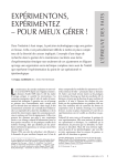
Figure 4.1 shows a partially dened Pascal program named book. It consists of
many entities such as the types Integer, Real, and class; the procedures swap and
sort; and the objects list, i, and j . There are many dependencies between these
entities. For instance, the object list is of type class, the procedure sort calls swap,
and the type class references first and last. Such dependencies are determined
during the analysis of the code of the program.
Naturally, the set of entities of a program p and the dependency relation are
represented by a directed graph; a vertex2 of the graph represents an entity of the
program, and an arc represents a dependency relationship between the entities corresponding to the arc's vertices. For instance, if entity a depends on entity b and the
vertices a0 and b0 are their corresponding node representations, then the arc a0 !e b0
represents the relationship (a; b). If N is the set of vertices representing the entities
of program p and E is the set of arcs representing the dependency relation, then
G = (N ; E ) is a directed-graph representation of program p. We call G a program
dependency graph (PDG).
As remarked above, we denote the dependency relationship between the entity p
and entity q by the ordered pair (p; q). This representation does not depend on how
many times p uses q. For instance, if p is a procedure statement that references the
global variable q ten times, then this relation is represented by the unique ordered
pair (p; q). As a result, if p0 and q0 are the nodes representing p and q, respectively,
then there is exactly one arc p0!e q0 in the PDG. In general, we can say: if p0 and q0
are two nodes of the PDG, then there is at most one directed edge from one to the
other.
The directed graph of Figure 4.2 is a subgraph of the PDG that represents program book. The nodes n4, n5, and n6 represent the program entities class, list, and
sort, respectively. The arc n6 !e n12 represents (sort; swap), a relationship between
2
We use the terms \node" and \vertex" alternatively.
38
n1
book
n2
n3
first
n8
first
n4
last
n9
n5
class
n6
list
n10
n11
i
last
n 14
p
n13
swap
n 16
q
book.st
sort
n12
j
n 15
n7
temp
Figure 4.2: An Attributed Program Dependency Subgraph
sort.st
n 17
swap.st
39
the procedures sort and swap. Also the arc n5 !e n4 represents (list; class), the
relationship between the object list and its type class.
Embodied in this representation is the correspondence between the entities of the
program and the nodes of the graph. This correspondence is dened during graph
construction. If F is a function that designates the node associated with each entity,
then F is a one-to-one function from the set of entities of the program onto the set
of nodes of the PDG. Normally, each program entity is identied by a name, for
instance, procedure sort, type entry, or object last. We use such names to identify
the nodes of the graph by labeling each node with the name of the entity to which
it corresponds. When the distinction between the node and the entity is obvious, we
use such names to identify the nodes of the graph as well. Thus, one label of a node
n is going to be F ,1(n).
The identication technique we just described has a problem: there may exist
many dierent nodes that have the same label. In Figure 4.1, program book depends
on a pair of constants named first and last, and procedure sort depends on a pair
of parameters named similarly. So, the corresponding PDG (Figure 4.2) has two
dierent nodes (n2 and n8) that are labeled first and another similar set of nodes
(n3 and n9) that are labeled last. In Pascal programs, the problem is solved easily,
because within a particular context, only one of those similarly named entities is
known to exist. If a PDG preserves the structure of the programs they represent, we
can solve the naming problem in such a graph by specifying the context of the name.
Attributed Program Dependency Graphs
A PDG is an abstract view of a program without sucient details to generate
useful program views or to solve the problem of change analysis. Therefore, we keep
additional information as attributes of the nodes and arcs of the PDG. The level
40
of change analysis to be conducted determines the information to be retained. In
our approach, we choose information at the granularity level of procedures, functions, types, and variables. Although other information (such as the condition of a
while-do statement, the components of an if-then-else statement, or the structure of
an expression) is important for change analysis, we are leaving out such localized
information, with the hope that human analysts can easily get it from the textual
code. We would like to emphasize that an APDG is not an alternative to the code
of a program; an APDG complements its corresponding code. Thus, many times
we refer to the combination of the two representations of a program as the program's
graph-based representation.
An attributed program dependency graph (APDG) is a PDG whose elements
(nodes and edges) are attributed. In the following subsections, we describe the
attributes we assign to the nodes and edges of an APDG and discuss the reasons for
this assignment.
Node Attributes
A node attribute species a characteristic of the corresponding node's entity. For
Pascal programs, for instance, the following attributes can be used for the nodes of
the APDG:
A. Entity name
We use the name of the entity to label the entity's node; this label is one
attribute of the node.
B . Entity class
Another attribute of a node is the class of the node's entity. The entities of
the program dier in declaration/denition and use. In Pascal, we classify the
entities into four mutually disjoint classes:
41
A class of PROCEDURE entities (P )
P consists of the following subclasses:
{
{
{
{
programs,
procedures,
functions, and
procedure and function parameters.
A class of OBJECT entities (O)
O consists of four subclasses of entities:
{
{
{
{
constants (including values of enumerated types);
labels;
value, variable, and le parameters; and
variables.
A class of TYPE entities (T )
T consists of all of the following subclasses:
{
{
{
{
{
{
{
primitive types, integer, real, char, boolean, string, and le;
index types;
enumerated types;
sets;
arrays;
records; and
pointers.
A class of STATEMENT entities (S )
S consists of entities each of which corresponds to the statement part of
a subprogram. In this thesis, we consider the outermost begin-end compound statement of a procedure, a function, or the program as its state-
42
ment entity. We name this entity as the name of its parent subprogram
concatenated with the string \.st".
Entities of a class have similar characteristics, but entities of dierent classes
dier in denition and purpose. To preserve the properties of these classes, the
nodes of the corresponding APDG are similarly divided into four classes. Let
G (N; E ) be an APDG and F its dening function.
Let also,
No = F (O),
Np = F (P ),
Ns = F (S ), and
Nt = F (T )
then
N = No [ Np [ Ns [ Nt and
No, Np, Ns , and Nt are pairwise disjoint.
We call the nodes of No, o nodes; the nodes of Np, p nodes; the nodes of
Ns, s nodes; and the nodes of Nt, t nodes. In this thesis, we use icons of
dierent shapes to distinguish between nodes of dierent classes. We use oval
icons for o nodes, parallelogram icons for p nodes, square icons for s nodes,
and triangular icons for t nodes.
In Figure 4.2, the nodes n2; n8, and n14 are in No; they are o nodes. The nodes
n1; n6, and n12 are in Np; they are p nodes. The nodes n7; n13, and n17 are in
Ns; they are s nodes. The node n4 is in Nt; it is a t node.
C . Entity context
Many languages allow the use of dierent entities of the same name in dierent
43
contexts; they provide scope rules to resolve references to these names. (The
scope rules usually describe what entities can be referenced at a particular
point of the program.) To apply the scope rules, the context has to be made
available. We have to use additional node attributes to describe the contextual
information of the corresponding entity. This information will then be used
not only to solve the naming problem, but also for change analysis.
In high-level languages, the order in which the entities of a program are declared/dened is very important. For example, one procedure cannot call another unless the latter is declared rst. It is possible to include this ordering
in the graph representation of programs. Let n1, n2, n3, : : :, nk be a sequence
of entities of a given program that are declared at the same level of nesting
within the block of entity n and in this given order. Then one way to preserve
this ordering is to link their corresponding graph nodes n01, n02, n03, : : :, n0k into
the parent node n0 (that represents n) in the same order. The order of the
siblings n01, n02, n03, : : :, n0k will be the same as the order in which the given
entities are declared within n. We keep the original position of a sibling as
a node attribute. This ordering preserves the static organization of the entities of the programs being represented, which in turn is very important to the
interpretation of scope rules of the language.
D. Entity locations
An APDG complements the code of its program. The linkage between the two
representations must be available so as to access one representation from the
other. We keep the locations where an entity is declared/dened and referenced
as node attributes.
44
Edge Attributes
The dependency relation between the entities of the program is an abstraction of
several dierent relations. Subprograms dene their own local entities, use parameters to communicate with others, and reference other global entities. Record types
use eld selectors to identify the components of their values. Objects are declared
to be of previously dened types. These relations have dierent semantics. It is
logical to partition the dependency relation into several distinct classes. For Pascal,
we partition this relation into three classes:
A class of LOCAL dependencies (L)
L consists of all pairs (p; q) such that either p is a record type and q is one of
its components, or q is an entity that is declared within the block of p and p is
a procedure, a function, or a program entity.
A class of PARAMETRIC dependencies (C )
C consists of all (p; q) such that p is either a procedure or a function or a
program and q is one of p's formal parameters. That is, C includes all pairs
(p; q) such that q is a formal parameter of p, where p 2 P .
A class of REFERENCING dependencies (R)
R consists of all (p; q) such that
{ p is an object or a function and q is p's type;
{ p is a type that references type q; or
{ p is a statement entity that references q, where q is an object variable, a
procedure, or a function.
If desired, references to variables can be further rened into two subclasses:
read references and write references. This helps data-ow analysis.
45
The three classes L, C , and R are mutually disjoint.
In Figure 4.1, the pairs (i; Integer), (sort:st; list) and (p; Real) are in R. Meanwhile, the pairs (sort; last) and (swap; p) are in C ; and the pairs (sort; i), (sort; swap)
and (book; class) are in L.
The elements of a dependency relation are represented by the arcs of the APDG.
Hence, we partition these arcs into three subsets as well.
Let
e
E1 = fF (p)!F
(q) j (p; q) 2 Lg,
e
Er = fF (p)!F
(q) j (p; q) 2 Rg, and
e
Ep = fF (p)!F
(q) j (p; q) 2 C g,
then
E = El [ Ep [ Er and
El \ Ep, El \ Er , and Ep \ Er are empty sets.
We label each arc of the graph using the initial of the relation it belongs to. So, if
a!e b is in El, Ep, or Er then its label is going to be l, p, or r, respectively, and we
refer to this arc as a!l b; a!p b, or a!r b. In Figure 4.2, the edges n1 !e n2, n6 !e n10,
and n12!e n17 are l edges; the edges n5!e n4, n13!e n9, and n17!e n14 are r edges; and
the edges n6!e n8; n12!e n14, and n12!e n15 are p edges. Notice that we use arrows of
dierent widths to dierentiate between these edges; we use thin arrows to represent
p edges, thick arrows to represent l edges, and dotted arrows to represent r edges.
The class of the edge is an attribute of this edge.
Graph Operations
Graph operations are the only operations that can manipulate the APDG G .
46
Their implementation depends on the way the APDG is represented. Following is a
sample list of these operations and their usage:
CreateNewNode(n; c)
This operation creates a new graph node of class c for entity n.
AddNode(G ; n; l)
This operation adds node n to a given graph G at a given location l.
DeleteNode(G ; n)
This operation deletes the given node n from the graph G .
GetNode(G ; e; c)
This operation nds the node corresponding to entity e in the context of entity
c in the APDG G . This function returns n = F ,1(e), where F is the dening
function of the APDG G .
AddEdge(G ; u; v; c)
This operation adds an arc u!c v to the APDG containing the nodes u and v.
DeleteEdge(G ; u; v)
This operation deletes the arc u!e v from the APDG containing the nodes u
and v.
IsEdge(G ; u; v)
This Boolean function checks whether there is an arc u !e v in the APDG
containing the nodes u and v.
Other operations are used to assign attributes to the nodes of an APDG, get information about a given node, and so forth.
As shown in Figure 3.1, all SCAN operations interact with an APDG using these
graph operations. Thus SCAN components do not depend on the way an APDG is
implemented.
CHAPTER V
GENERATING ATTRIBUTED PROGRAM
DEPENDENCY GRAPHS
The APDG Generator is a set of operations that generates the APDG representation of a program from the program's code. These operations are similar to
a compiler's operations: they syntactically analyze the program's code. However,
instead of generating a syntax tree, they generate an APDG. We have implemented
a prototype Graph Generator for syntactically correct Pascal programs. The prototype's operations are based on high-level algorithms several of which are given in
this chapter.
Notations Used in the Graph Generator Algorithms
Before describing the graph-generating algorithms, we describe the notations used
in these algorithms. These notations are C-like, since the prototype graph generator
was implemented in C. We use while statements, if-then-else statements, repeat-until
statements, functions, return statements, and so forth. However, because we are
describing high-level algorithms, mathematical set notations are used as well. Also,
for convenience and clarity, we use square brackets instead of curly brackets. All
comments end with end-of-line marks.
47
48
Most algorithms are described in a way that makes them easy to understand.
However, these descriptions are not detailed enough to include descriptions of primitive processes, especially those that are related to graph implementations.
In addition to the operations listed in Chapter 4, we use a queue data type with
three operations:
EmptyQueue(L)
This Boolean function checks if the queue L is empty.
AddQueue(L; u)
This operation adds u to the tail of queue L.
DeleteQueue(L)
This function returns the head of the queue L and deletes that element from
the queue.
Lexical Analysis
A lexical analyzer is a fundamental operation of graph generation. Given the code
of a program, the lexical analyzer reads the text characters and produces a sequence
of meaningful tokens according to the specications of the programming language.
For each token, the lexical analyzer species the token's name, type, and location;
these are valuable for later analysis.
In the graph generating algorithms, we use the function NextIdentifier, a function that extracts the next identier from the code of a program using a lexical
analyzer. NextIdentifier searches through the sequence of tokens of the program
that is generated by the lexical analyzer, until it nds an identier and returns the
combination of the identier's name and location as its value.
49
Generating APDGs for Pascal Programs
The structure of a program and that of a procedure are similar. A program or
procedure consists of two parts: a heading part and a block part. The name of
the program/procedure and its parameters are described within the heading part;
meanwhile, local entities, such as types, objects, and procedures, are declared in the
block part. The block also includes the statement part of the procedure, where many
entities are referenced. The same syntax rules1 are used to declare any entity, whether
it is a component of a procedure or a component of a program. Thus, programs and
procedures have similar graph generators. We describe here one process to construct
the APDG representation for any procedure.
In the following subsections, we describe GraphProcedure, a process for generating an APDG representation of a syntactically correct procedure. GraphProcedure,
incrementally constructs the subgraph and adds it to the APDG at a specied location. For this we assume the existence of an APDG G = (N ; E ), where N is the set
of the graph nodes and E is the set of its arcs.
The denition of GraphProcedure is a direct result of the syntax rules of Pascal.
We develop this denition in a top-down manner that mirrors the way these rules
are specied. Two points should be emphasized here:
We are not describing a new approach to syntactical analysis of Pascal programs; we are discussing the actions that accompany the analysis process.
We are not writing a complete design for an APDG generator; we are describing, in a high-level-like language, how to generate the APDG for major
constructs of Pascal.
1
All relevant syntax rules are listed in the Appendix in BNF notation.
50
Let us start with the top-most rule that describes the structure of a procedure
h procedure declaration i ::= h procedure heading i h block i:
In abstract terms, GraphProcedure (we are not including a denition of it here)
consists of two main modules: GraphProcedureHeading and GraphProcedureBlock.
As the names may suggest, the rst module creates the subgraph of the procedure
heading and the second module creates that of the procedure block. GraphProcedureHeading adds all nodes that represent the procedure identier and its formal
parameters to the evolving APDG. It also adds the necessary arcs to the APDG.
GraphProcedureBlock adds more nodes (such as those representing local entities) and
more arcs (such as those representing local or global references) to the APDG.
Generating an APDG for a Procedure Heading
A procedure heading (see the Appendix for related syntax rules ) consists of a
procedure identier and a list of formal parameter sections. There are two types of
parameters: object parameters and subprogram parameters. Type parameters are
not allowed in Pascal. We do not intend to completely dene GraphProcedure here;
instead we describe its major components.
As the syntax rules suggest, there are two components to consider: StartProcedureHeading and FinishProcedureHeading. The rst deals with the procedure identier, and the second deals with the procedure parameters.
StartProcedueHeading extracts the procedure identier from Pascal code, creates
a node representation for this procedure, and appends this node to the APDG.
Assume that a procedure v is declared within the block of procedure u and that u0
represents u. StartProcedureHeading creates a p node (v0) to represent v and links v0
to u0 by the arc u0!l v0.
51
FinishProcedureHeading( G ; u )
APDG G = (N ; E );
GraphNode u;
/* This algorithm completes processing the heading part of the procedure u;
/* it processes the formal parameter list. For each procedure parameter s, it
/* adds one p node to the graph G and links this node with u by a p edge.
/* Otherwise, it adds an o node and two edges: a p edge to link the
/* parameter to u and an r edge to link the parameter to its type.
/* Function parameters are represented by p nodes and are linked to
/* their corresponding types by r edges.
[
GraphNode s; t;
Identifier id;
String NodeClass;
Queue of Identiers L;
For each parameter section in a parameter list
[
If parameters are procedures/functions
NodeClass=\p node";
Else NodeClass=\o node";
L = ;;
Repeat
id= NextIdentier();
/* id of a parameter
s = CreateNewNode (id; NodeClass); /* N = N [ fsg
AddEdge (G ; u; s; p);
/* E = E [ f u!p s g
AddQueue(L; s)
/* Save ordering of declarations
Until end of identiers list;
If
]
]
parameters are not procedures
[ /* Get the type of the parameters' section.
t = GetType();
/* Link all parameters in this section to their type q
Repeat
s = DeleteQueue(L);
/* Get them in order of declaration
AddEdge(G ; s; t; r);
/* E =E [ f s!r tg
Until EmptyQueue(L)
/* L == ;
]
Algorithm 5.1: FinishProcedureHeading
52
FinishProcedureHeading (Algorithm 5.1) extracts the formal parameters of a
procedure and builds their subgraph representation. Two types of nodes could be
added to this graph. The rst type consists of o nodes that represent object parameters. Each node is linked to the procedure node by a p edge, and linked to the
object type node by an r edge. The second type consists of p nodes that represent
procedure parameters. Each one is to be linked to that of the node of the parent
procedure by a p edge. A function parameter is represented by p node. But, unlike a procedure parameter, it has a type. So the node representation of a function
parameter must be linked to its type node by an r edge.
As an example, consider the heading of the following procedure sort: ( This is
declared in the main block of program book, Figure 4.1.)
procedure sort ( first ; last : Integer);
StartProcedureHeading adds a p node to represent procedure sort and links the node
to book by the arc book !l sort. Then FinishProcedureHeading creates two other
o nodes to represent the parameters first and last, and links them to sort by two
p edges sort!p first and sort!p last. It also adds two r edges, first!r Integer and
last!r Integer, to represent the relationships between first and last and their type
Integer. These additions are illustrated in Figure 5.1.
53
book
Integer
sort
first
last
Figure 5.1: An APDG of a Procedure Heading
Generating an APDG for a Procedure Block
The top-most syntax rule of a procedure block is as follows:
h block i ::= h label declaration part i h constant declaration part i
h type denition i h variable declaration part i
h procedure declaration part i h statement part i
As shown, the block of a procedure contains the declarations of any new local types,
variables, and procedures. It also contains the statement of the procedure. We dene GraphProcedureBlock to create the corresponding subgraph of any block. Since
the parts of a procedure block are not similar, the block component of a procedure
is more complicated to graph than its heading. So GraphProcedureBlock is longer
54
and has more components than its twin algorithm GraphProcedureHeading. These
components are GraphLabel, GraphConstant, GraphType, GraphVariable, GraphProcedure, and GraphStatement. To concentrate on the components themselves, we are
not including any sketches of GraphProcedureBlock. Instead, we describe an algorithm to create the subgraphs of major parts of a procedure block independently
from the other parts. We describe one algorithm to graph array-type denitions,
a second to graph record-type denitions, a third to process variable declarations,
and a fourth to complete the subgraph by processing the procedure statement. As
for new local procedures, we use, recursively, the algorithm GraphProcedure that is
being dened.
Type Subgraphs
As described by Pascal syntax rules, types in Pascal may be standard or userdened. Standard types are integer, real, char, and boolean. The properties of
these types are determined by the Pascal language implementation. We will therefore
assume that there is no need to redene them, and that they are local entities of the
standard environment of the whole program. (This is the rst instance of a multile program.) Such standard entities are used by other entities, implying that their
corresponding graph nodes are leaf nodes; i.e., the out degree of each node is zero.
Users can redene such identiers. In such a case the redened entity gets a new
meaning. The corresponding graph node is not going to be a leaf node. Its direct
successors will describe its new structure.
User-dened types are classied into two groups. The rst group includes subranges, sets and scalar types. The second group includes the structured types;
namely, arrays and records. These types are among the most important features
of high level languages including Pascal. In the following subsections, we describe
55
two algorithms, GraphArrayType and GraphRecordType, to construct the subgraphs
of array and record types respectively.
Array Subgraphs
The syntax rules of an array type denition are as follows:
h array type i
::= array [ h index type i ] of h component type i
h index type i
::= h simple type i
h component type i ::= h type i
GraphArrayType (Algorithm 5.2) creates the subgraph that corresponds to any
array type denition. The structure of this algorithm is a direct result of the above
rules. It always adds references from the array node to all indexes and to the components' type.
As an example, consider the following declaration of the array type list: ( This is
declared in the main block of program book, Figure 4.1.)
list = array [first::last] of Real
where list is the array type, rst..last is an index range which implements a type,
and Real is the component type. GraphArrayType creates a t node to represent the
array list, then it calls GraphType to draw, in this case, the subgraph of the index
type first::last. GraphType will create a t node, name it \list:index", and add it
as a local entity of book. In this case, GraphType adds the arcs book !l list:index,
list:index !r first, and list:index !r last to the graph G . GraphArrayType also
adds the arcs list!r list:index and list!r Real to the program graph G . Figure 5.2
illustrates the resulting subgraph.
Notice that array types are dened by referencing other types.
56
GraphArrayType (G ; u)
APDG G = (N ; E )
GraphNode u;
/* Parent of the entity being dened
/* This algorithm gets the array identier, all index types,
/* and the components' type. It then, adds referencing edges
/* from the array node to all nodes of referenced types.
[
GraphNode t; s;
Identier id;
/* Get the array identier and create its node representation.
id = NextIdentier();
t = CreateNewNode(id; t node); /* N = N [ ftg
AddEdge(G ; u; t; l);
/* E = E [ f u!l t g
/* Get (or create) the node representation of each index and reference it.
For each array index
[ s = GetType();
/* Get the index type.
AddEdge(G ; t; s; r); ]
/* E =E [ f t!r s g;
]
/* Get the node representation of the components' type and link
/* the new array node (t) to this node by an r edge.
s = GetType();
/* Get the components' type.
AddEdge(G ; t; s; r);
/* E = E [ f t!r s g;
Algorithm 5.2: GraphArrayType
57
book
Real
first
last
list.index
list
Figure 5.2: An APDG of an Array Type
Record Subgraphs
A record entity consists of several elds the types of which are not necessarily
the same. Here are the syntax rules of those record types.
h
h
h
h
record type i
eld list i
record section
eld type i
::= record h eld list i end
::= h record section i f ; h record section i g
i ::= h eld identier i f ; h eld identier i g : h eld type i
::= h type i
58
A record entity consists of many record sections; within each section, a group of
one or more eld identiers are declared to be of the same type. GraphRecordType
(Algorithm 5.3) constructs the subgraph associated with any record type. For each
section, it collects the eld identiers, keeps them in a queue, and then nds their type
entity. Then, GraphRecordType creates their corresponding node representations and
links each of these nodes to the record type node by l edges. Finally, it links these
nodes again to their type node by r edges. The use of the queue here saves the order
of the declarations of the elds so as to link them in that order.
As an example, consider the declaration of the record type entry as a local entity
of the program book:
entry = record
name, address : String;
grades : scores;
total : Integer;
end;
This record consists of three record sections, the rst of which has two eld
identiers while each of the others has only one eld identier. GraphRecordType
creates a t node to represent entry itself and links this node to book's node by an
l edge. It creates also four o nodes to represent the eld selectors name, address,
grades, and total, respectively, and links these nodes to node entry by the edges
entry!l name, entry!l address, entry!l grades, and entry!l total. GraphRecordType
links also the four eld nodes to their corresponding types by the arcs name!r String,
address !r String, grades !r scores, and total !r Integer. Figure 5.3 illustrates the
resulting APDG of the record entry.
59
GraphRecordType(G ;u);
GraphNode u;
APDG G = (N ; E );
/* For each declaration section of a record type t, this process gets a
/* queue L of all eld selectors in a this section and their type s.
/* Then, it creates an o node for each eld selector and links
/* this node with two arcs to the procedure node u and the type node s.
/* Th queue is used to reserve the ordering of the elds of the record.
[
GraphNode p; s; t;
Identifier id;
Queue of identiers L;
/* Represent the record type entity.
id = NextIdentier();
t = CreateNewNode( id; t node );
AddEdge(G ; u; t; l);
/* N =N [ ftg
/* E = E [ f u!l t g
Repeat
/* Process each identiers list
/* Get the identiers list of this section.
L = ;;
Repeat
id = NextIdentier();
/* N = N [ fpg;
p = CreateNewNode(id; o node);
AddQueue ( L; p);
Until all eld identiers are processed;
]
/* Get the type of all elds in this section
s = GetType();
/* Create the subgraph representation of this section.
Repeat
p = DeleteQueue( L );
AddEdge(G ; t; p; l);
/* E = E [ f t!l p g
AddEdge(G ; p; s; r);
/* E = E [ f p!r s g
Until EmptyQueue( L );
/* L == ;
Until end of the current declaration part;
Algorithm 5.3: GraphRecordType
60
book
Integer
String
scores
entry
name
address
grades
total
Figure 5.3: An APDG of a Record Type
Variable Subgraphs
In any block, the variable declaration part consists of many sections. In each
section a group of identiers are declared to be of the same type. Here are their
syntax rules:
h variable declaration i ::= empty
j var h declaration section i f ; h declaration section i g
h declaration section i ::= h identier i f ; h identier i g : h type i
61
When compared to the declaration sections of a record type, one nds that although the names of the constructs are dierent their meanings are the same. Assuming that GraphVariable is a process that builds the graph representation corresponding to any variable declaration section, it is going to be similar to GraphRecordType
(Algorithm 5.3). (Actually, this latter algorithm is built using GraphVariable.) The
only dierence is that all variable nodes are linked to a p node rather than to a
t node as in record types. We shall not write this algorithm; however, we would like
to emphasize that GraphVariable constructs the graphs associated with the declaration sections and appends them to the APDG. For each variable identier an o node
and two arcs are added, one arc to represent the local relationship between the block
and the identier, and the other to represent the referencing relationship between
the identier and its presumed global type.
Procedure Subgraphs
If the procedure declaration part of a block is not empty, then for each procedure
within it, GraphProcedure is called recursively. The recursive calling sequence is
nite because procedure nesting is nite in Pascal.
Statement Subgraphs
Normally, the statement part of a procedure is a compound statement. It consists of a combination of simpler statements that are constructed from assignment
statements and procedure (or function) calls. No declarative statements are allowed
here, which means that no new entities are declared in a statement part. Entities
referenced by a statement are either previously dened by the programmer or by the
language implementation.
62
In APDGs, the statement part of a procedure is considered a STATEMENT
entity that references all entities used in this part. A STATEMENT entity is represented by an s node, and all references in its corresponding statement part are
represented by r edges incident from this s node. All nodes adjacent to an s node
are either o nodes or p nodes.
To complete the subgraph of a procedure, the operation GraphStatement (Algorithm 5.4) creates an s node to represent the statement part and adds it to the
graph by linking it to the procedure node by an r edge. The name given to this
node is the name of the parent procedure concatenated with the string \.st". After
this, the process goes through the statement, iteratively, looking for all entities being
referenced. For each of them, GraphStatement adds one r edge from the s node to
the referenced node.
As an example, consider the statement of procedure sort as dened in Figure 4.1:
Begin
For i := first to last , 1 do
For j :=i+1 to last do
If list[i] > list[j ]
Then swap(list[i]; list[j ])
End;
GraphStatement rst creates an s node to represent sort statement, names it as
sort:st, and links it to the node sort by the arc sort!l sort:st. Then, GraphStatement
iterates through the sequence of tokens searching for program entities, and when it
nds an entity t, it adds a referencing arc from s to t (if it is not already there)
and updates the list of locations of t. Figure 5.4 illustrates these additions to the
evolving APDG.
63
GraphStatement(G ; u);
GraphNode u;
G = (N ; E );
/* This algorithm creates a s node representation (s) for the statement part
/* of procedure u. It then iterates through the statements of this part
/* looking for references to other entities. GraphStatement links the
/* node s to each of them by an r edge.
[
GraphNode s; p;
/* s is the statement node.
Identifier id;
/* First, create a node representation for this statement.
id:name= u.name+\.st";
/* Make a statement name
s = CreateNewNode(id; s node); /* N = N [ fsg;
AddEdge(G ; u; s; l);
/* E = E [ f u!l sg;
/* Second, for each referenced entity inside this statement part,
/* add a reference from the statement node to referenced node and
/* update locations list of the referenced node to incorporate the
/* new locations.
Repeat
id= NextIdentier();
p= F (id);
/* p is a previously dened entity.
AddEdge(G ; s; p; r);
/* E = E [ f s!r p g
Until the end of the statement;
End
Algorithm 5.4: GraphStatement
64
1
list
sort
first
last
i
j
Figure 5.4: An APDG of a Statement
swap
sort.st
CHAPTER VI
A GRAPH-BASED REPRESENTATION FOR
MULTIPLE-FILE PROGRAMS
Many programming languages allow the division of programs into several les
that can be separately compiled and later linked together. In these multiple-le
programs, entities of one le may depend on entities dened in another le. For
example, procedure p in le a may call procedure q that is dened in le b. In this
example, procedure p references q; le b depends on procedure q; and le a indirectly
interacts with le b. We summarize these interactions by saying that le a imports
procedure q from le b (or le b exports procedure q to le a). To be of practical
use, a software change analyzer must handle such inter-le interactions in addition
to the intra-le interactions that we discussed earlier. In this chapter, we extend the
graph-based representation of our approach to accommodate inter-le interactions.
We carry out this extension in two steps:
1. Extend the APDG representation to retain information about interactions between dierent les of a multiple-le program and their entities. This may
require introducing new entities, graph nodes, attributes, or relationships. We
refer to the resulting graph as an extended APDG.
2. Modify the graph generation process so that it collects inter-le information
65
66
(in addition to the intra-le information), and saves it in the extended representation.
APDGs for Multiple-File Programs
A typical large software system normally consists of many les each of which can
be separately compiled. A compiler (of the programming language used in writing
the system) analyzes the structure of a le by getting specic information about
all entities imported by this le. Although each programming language has its own
strategy for specifying how a le can import entities from other les (or export entities
to them), all languages require that every le that imports an entity must include a
mimic declaration of this entity. Using this information, the compiler checks whether
all references to the imported entity are consistent with this mimic declaration. The
linking loader checks whether all mimic declarations of an entity in dierent les are
consistent with its actual declaration/denition.
To analyze multiple-le programs, we modify the graph-based representation that
we described in Chapters 4 and 5 as follows:
Introduce a new class of FILE entities.
We consider each le of a program as an entity of this program and dene a
new class (FILES) of these new entities. We represent each FILE entity by a
graph node whose class is an f node. Accordingly, the graph representation of
a multiple-le program will have as many f nodes as it has separate les.
Dene the relationships between a FILE entity and its components.
Consider all declarations (even declarations of imported entities) local to the
FILE entity that contains them. This means that the relationship between
a FILE entity and its major components (i.e., the program entities that are
67
declared/dened at the top-most level of this le) are LOCAL relationships.
Thus, all arcs incident from an f node are l edges. Notice that the node
representation of any FILE entity is the top node of the APDG of the le and
it will be the only entrance to access this graph.
Represent each le by a separate APDG.
Since all references within a le are resolved by intra-le information (especially
after declaring every imported entity in the le), this le can be represented
independently from others by an APDG. The set of all APDGs is the nucleus of the graph-based representation of any multiple-le program. This
multiple-graph representation inherits the advantages of dividing a program
among multiple les. So instead of constructing a gigantic graph, we construct
a set of easy to create, easy to manage, and easy to access subgraphs. Another
advantage of this multiple-graph representation is that not all graphs need to
be kept in internal memory at one time.
Let us emphasize that a global entity must have a corresponding node representation in each APDG of the le that imports or exports this entity.
Use a node attribute to specify the le from which the entity is imported.
An optional node attribute that describes the le where an imported entity is
actually declared can be used. If, for instance, variable a is imported from le
b, then b is the value of the le attribute of node a. The le attribute is not
necessary for local entities that are not exported from the le; this is the name
of the top node of the graph that includes the local node.
Given an extended APDG1 of a le a, it is possible to determine the set of
les that le a imports from, by checking the le attributes of the nodes of APDG.
However, to answer the question \which les does le a export to" is time-consuming,
1
We will drop the term extended from now on.
68
because we have to repeatedly check the le attributes of each APDG and nd
which les import from a. However, considerable cost reductions can be achieved by
keeping, for each le, a listing of all les that import from it. Similar reductions can
be achieved if, in addition, a listing of all exported entities and the les where they
are dened {each entity is dened in exactly one le{ is kept. For later use, we refer
to these two listings as export-to and dened-in tables.
Since export-to and dened-in table listings describe binary relations among the
entities of a multiple-le program, they could be represented by graphs in the same
way that dependency relations were represented. However, this makes all APDGs
look connected and appear as a gigantic graph, which we wish to avoid for scalability
reasons.
Generating APDGs for Multiple-File Programs
The process of generating the APDG of a le of a multiple-le program is a
slightly modied version of the graph generator that we described in Chapter 5. The
modications are necessary to generate the extended forms of the APDG. These
modications are as follows:
The rst step of graph generation is to retrieve the relations export-to and
dened-in; these tables can be updated if the program le being graphed im-
ports entities from other les.
The graph generator must create an f node for each le it graphs. The node
representation of every major construct of this le must be linked to this f node
by an l edge.
Graph generation then proceeds as described in the previous chapter except
when an import declaration is encountered; the graph generator must then add
69
an entry that characterizes this inter-le relationship to the export-to table.
When the graph generator processes the declaration/denition of an exported
entity, it must add an entry, that describes the association between this entity
and its le, to the dened-in table.
When the le ends, the graph generator must save the APDG and the two
updated versions of the relations export-to and dened-in.
We call the combination of the APDGs, export-to and dened-in tables, and
the code of a multiple-le program, a graph-based representation. We illustrate
the graph-based representation of a multiple-le program and the method of its
generation using Berkeley Pascal [Joy et al., 83].
Multiple-File Programs in Berkeley Pascal
Berkeley Pascal is an extension of Standard Pascal in which a program consists
of one or more les. In a multiple-le program, one le must be the main le (this
le contains the main program), and the other les are either header les or unit
les. Global entities (such as constants and types), are dened in header les; also,
global variables and external procedure or function interfaces are declared in header
les. An external procedure or function must be dened in one unit le only. To
use a global entity in le a, a must include (using an include-statement) the header
le that contains the entity's declaration/denition. The header le that contains
an external procedure declaration must be included in every le that references this
procedure and in the unit le that denes procedure. The same rule must also hold
for functions. This set of rules species how a le can import entities from other
les.
Figure 6.1 illustrates a multiple-le program in Berkeley Pascal. It is similar
70
| a.h |
Const
rst= last = Type
class=Array[rst..last] of Real;
| b.h |
Procedure swap(Var p; q :Real);
External;
| unit.p |
#include \b.h"
Procedure swap;
Var
temp: Real;
Begin
temp :=p;
p := q ;
q := temp
End;
| main.p |
Program book ( );
#include \a.h"
#include \b.h"
Var
list : class;
Procedure sort ( rst,last:Integer );
Var
i; j : Integer;
Begin
For i:=rst To last-1 Do
For j := i + 1 To last Do
If list[i] >list[j ]
Then swap (list[i];list[j ])
End;
Begin
...
sort(rst,last);
...
End.
Figure 6.1: A Multiple-File Program in Berkeley Pascal
71
to program book as described in Chapter 3; but it is divided among four les: two
header les, a unit le, and the main le. In this program, the entities rst, last and
list are global entities; these are dened in the header le a.h. The procedure swap
is external to the main program le and is dened in the unit le unit.p. The Swap
interface is dened in the header le b.h which is included in both les unit.p and
main.p.
Example APDG of a Berkeley Pascal Program
Let us discuss the major steps that a graph generator must take to construct
the APDGs of program book. These steps are applications of the guideline rules we
described for graphing multiple-le programs.
Get the inter-le tables import-to and dened-in. These could be empty if no
graphs have been generated yet or no imports have been declared. For Berkeley
Pascal, we dene an alternative table to the export-to table; this new table lists
all les that include a given one. We call this new alternative the included-in
table. By doing so, we ease the construction of the included-in table without
losing any information that an export-to table could contain.
For each program le, the graph generator must create a new f node and assign
the available attributes (such as the node's name and class) to this node.
If le a includes le b, then after interpolating a copy of b into a and generating
the APDG of the extended le a, we must be able to recognize the entities of
the graph of a that are declared/dened in b. This is done by assigning b to
the le attribute of each of b's entities.
Moreover, the relationship between b and a must be saved; this is done by
adding an entry that describes this relationship to the included-in table.
72
If le a is a unit le that contains the denition of the external procedure b
and le c is the header le that contains the declaration of b, then le a must
contain a mimic declaration of b and its actual denition. Recall that le a must
include le c so that le a can export b. The mimic declaration of procedure
b results from processing le inclusions. We represent both declarations in the
APDG of the unit le a.
Also, the relationship between le a and procedure b must be kept in the table
dened-in table.
Other than these special cases, graph generation proceeds as if the program is
a single-le one. Recall that all references are resolved internally.
Applying these guidelines to the program book shown in Figure 6.1, there will be
a set of four dierent APDGs that correspond to the four les of book. Figure 6.2
shows the APDGs of the les a.h, b.h, and unit.p, respectively. The APDG of the
main program le is not shown here. It is similar the graph shown in Figure 4.2.
The APDGs of Figure 6.2 has the following characteristics:
The APDGs are mutually disjoint.
The new le entities are represented by pentagons. These nodes are the top
nodes of their corresponding graphs.
All edges from top nodes are l edges.
The APDG of the unit le unit.p includes a subgraph that is similar to the
APDG of the header le b.h: both graphs have the nodes swap, p, q and Real
and the edges swap !e p; swap !e q; p !e Real, and q !e Real. Also, copies of
the graphs of a.h and b.h must appear as subgraphs of the graph of main le
main.p.
73
Figure 6.2: The APDGs of a Multiple-File Program
74
The inter-le relationships are not shown in those graphs, though such information is contained in them. Instead of deriving such information (and taking advantage
of its small size), we save it in tabular forms as shown in Table 6:1.
header le included-in
a.h
main
b.h
main
b.h
unit
global entity dened-in
rst
a.h
last
a.h
class
a.h
swap
b.h
Table 6.1: Sample Inter-File Relationships
This extended representation describes all entities of the program and the interactions between them whether these interactions are between local entities of a single
le or between entities of dierent les. We base the construction of the computer
assistant for change analysis on this information.
CHAPTER VII
CONSTRAINTS OF ATTRIBUTED PROGRAM
DEPENDENCY GRAPHS
An attributed program dependency graph has special properties that constrain
the graph's structure. We call these properties graph rules and keep them in a special
Rules Base. (See Figure 3.1.) There are two types of rules: general rules (that hold for
any APDG regardless of the programming language used to implement a program)
and specic rules (that hold for only APDGs corresponding to programs written in
a particular language). In this chapter, we discuss many examples of these rules.
Since we applying our approach to Pascal programs, we mark Pascal-specic rules
by an asterisk that precedes any of these specic rules.
In the following sections, we present many rules that hold for one APDG. To
study these rules, we assume the existence of a set of APDGs corresponding to
a multiple-le software program and generated according to the graph-generating
strategy we described in the previous two chapters. We assume also that each graph
G is (N ; E ), where N is a set of nodes and E is the set of arcs/directed edges. The
set of nodes N is partitioned into ve subclasses: Nf , No, Np, Ns, and Nt. This
classication is done according to the class attribute of the entities of the program.
The set of edges E is also partitioned into three subclasses: El , Ep , and Er . This
classication is done according to the type of the relationship (if any) that exists
between any two entities of the program.
75
76
Sample Attribute-Related Rules of APDGs
Following is a sample of the properties that hold for the attributes of any APDG:
A:1 The subclasses Nf , No, Np, Ns, and Nt are mutually disjoint.
The corresponding entity of each node has exactly one class attribute that the
node inherits. Since nodes are classied according to this attribute, each node
belongs to exactly one class.
A:2 The subclasses El , Ep, and Er are mutually disjoint.
As for nodes, each arc has exactly one attribute that characterizes the relationship between the arc's source and target nodes.
A:3 * If n 2 N and 9v 2 N such that v!e n 2 Ep, then 8m; m 2 N ; m 6= n, and
v!e m 2 Ep, name(n) 6= name(m).
(If m and n are parameters of p, then they must have dierent name attributes.)
No two parameters of the same procedure have the same name attribute.
A:4 * If n 2 N and 9v 2 N such that v!e n 2 El and 9m 2 N ; m 6= n such that
v!e m 2 El and name(n) = name(m); then
(1) v 2 Nf ;
(2) n; m 2 Np; and
(3) 6 9u 2 N u 6= m; u 6= n such that v!e u 2 E and name(n) = name(m) =
name(u).
(If n; m are two siblings | LOCAL components | of a node p and have the
same name attribute, then p must be a f node, n and m are p nodes, and no
other siblings have the same name.)
This is one constraint on dening an external PROCEDURE entity.
The following sections include other attribute-related properties.
77
Adjacency-Related Rules of APDGs
By analyzing the adjacency relations between the nodes of an APDG, one realizes
that nodes of some classes cannot be adjacent to1 nodes of other particular classes.
For instance, an o node cannot be adjacent to another o node, a p node cannot be
adjacent to another t node, and any node can be adjacent to a p node. The following
properties describe many relationships that hold between the nodes of an APDG:
Adjacency Relationships of an f node
A f node corresponds to a FILE entity. The following properties describe what nodes
can be adjacent to a f node and the types of these adjacency relationships.
B :1 9n 2 Nf ; that is, Nf 6= ;.
(Each APDG has at least one f node.)
When generating an APDG for any program le, the rst action a graph
generator does is to create an f node and associates it with this le.
B :2 If n 2 Nf and 9n0; n0 2 Nf , then n = n0
(There is at most one f node in every APDG.)
There is only one f node associated with each FILE entity of a multiple-le
program.
Actually, there is exactly one f node in every APDG.
B :3 If n 2 Nf , then 6 9m 2 N such that m!e n 2 E .
( A f node cannot be adjacent to any other node.)
Since n is a f node, it is not a local entity or a formal parameter of any
1
If p; q 2 N
and p!e q 2 E , then we say that p is adjacent to q, p!e q is incident
e
from p, and p!q is incident to q [Cormen et al., 90].
78
other entity of the program. Actually, other nodes are either linked directly to this node or to one of its successors. So there is no m such that
m!e n 2 Ep [ El. Moreover, n cannot be referenced by any node representing
an entity in the le n. As for references from other les, they are kept in the
e
export-to table. So, there is no m such that m!
n 2 Er .
As a result of these ndings, n is not adjacent to any other node of the graph;
this means that in degree(n) = 0. Thus, n is a top node of its APDG, and
since n is unique (Property B/2), n is the only top node of its APDG. We
often refer to this node as top.
B :4 If n 2 Nf and 9m 2 N such that n!e m 2 E , then n!e m 2 El .
(Every arc incident from an f node is an l edge).
This is true because a le of a multiple-le program does not reference any of
its own entities and does not have parameters. When we dened a FILE entity,
we assumed that all immediate components (that is, entities at the rst level
of nesting in this le) are LOCAL to this le. So their node representations
are adjacent to the f node by l edges.
Adjacency Relationships of an o node
An o node is a node corresponding to an OBJECT entity. The following properties
hold for any o node in APDG:
C :1 If n 2 No, then 9m 2 N such that n!e m 2 E .
(There is at least one node adjacent from an o node n).
An OBJECT entity (say n) must have a type (say m). Such relationship
between n and m is represented by the arc n!e m. So for any o node, there is
an arc incident from it.
79
C :2 If n 2 No and 9m 2 N such that n!e m 2 E , then n!e m 2 Er .
(Any arc incident from an o node n is a r edge.)
OBJECT entities are always simple; they do not have components or parameters. So, neither p edges nor l edges can be incident from an o node.
C :3 If n 2 No and 9m 2 N such that n !e m 2 Er , 6 9t; t 6= m; t 2 N such that
n!e t 2 Er .
(There is at most one node adjacent to an o node n by a r edge.)
Actually, there is exactly one node adjacent to n.
C :4 If n 2 No and 9m 2 N such that n!e m 2 Er , then m 2 Nt.
(An o node n can only reference t nodes.)
Normally, objects do not reference any entities other than type entities. This
implies that m is the only node such that n !e m 2 E . The out degree(n) is
one.
Adjacency Relationships of a p node
A p node is a node corresponding to a PROCEDURE entity. The following properties
hold for any p node in an APDG:
D:1 If n 2 Np and 9m 2 Ns such that n!e m 2 E , then n!e m 2 El .
(Given a p node n and there exists an s node m that is adjacent to n by the
edge n!e m, then n!e m is a l edge.)
This is a result of the fact that a statement of a procedure or a function entity
n is considered a local entity of n.
D:2 If n 2 Np and 9m 2 Ns such that n!l m 2 El, then 6 9o; o 6= m; o 2 Ns such
that n!l o 2 El .
80
(There is at most one s node that is adjacent to the p node n.)
A procedure or function has only one statement component.
D:3 If n 2 Np and 9m 2 N such that n!e m 2 Er , then m 2 Nt
(A p node can only reference a t node.)
By convention, PROCEDURE entities do not reference any other entities; their
components do the referencing. However a function entity can reference another
type entity when the type of the function is to be dened. This is the only case
when a PROCEDURE entity can reference another entity.
D:4 If n 2 Np and 9m 2 N such that n!e m 2 Er , then 6 9o; o 2 N , and o 6= m such
that n!e o 2 Er .
(If a p node n references the node m, then n does not reference any other node.)
If a PROCEDURE entity has a type, then this type is unique.
Adjacency Relationships of an s node
A s node is a node corresponding to a STATEMENT entity. The following properties
hold for any s node in the graph:
E:1 If n 2 Ns, then 9m 2 N such that m!e n 2 El .
(A s node is always incident from a l edge.)
Statements are always local entities of other entities.
e
E:2 * If n 2 Ns , and 9m 2 N such that m!
n 2 El, then m 2 Np.
(A s node can be only adjacent to a p node.)
In Pascal, no entity but a PROCEDURE entity has a statement component.
E:3 * If n 2 Ns and 9p; p 2 N such that n!e p 2 E , then n!e p 2 Er .
(An arc incident from a s node n is a r edge.)
81
In Pascal, a statement does not have locally dened components. Statements
are dened by referencing others.
E:4 If n 2 Ns and 9p 2 N such that n!e p 2 E , then p 62 Nt.
(If n references p, then p cannot be a t node.)
A STATEMENT entity cannot reference a TYPE entity.
Adjacency Relationships of a t node
A t node is a graph node that is associated with a TYPE entity. The following
relationships describe what nodes can be adjacent to a t node and the classes of
these relations.
F :1 * If n 2 Nt and 9m; m 2 N such that n!e m 2 E , then n!e m 2= Ep.
(A t node cannot have parameters.)
In Pascal, a TYPE entity cannot have parameters; it can have local components
such as a record type and it can reference other entities such as an array type.
F :2 * If n 2 Nt and 9m 2 N such that n!e m 2 E , then m 62 Np [ Ns.
(A t node n cannot be adjacent to a p node or an s node.)
In Pascal, types are dened by either dening local entities such as in records
or by referencing other objects or types such as in enumerated types and array
types.
Adjacency Relationships of a Generic Node
The following properties and relationships hold for any node in the graph:
82
e
G:1 If n 2 N and n 2= Nf , then 9m 2 N such that m!
n 2 Ep [ El
(For every n 6= top, there exists another node m such that n is adjacent to m
by either a r edge or p edge.)
The entity n is either dened/declared as a local entity of the le containing
n or as a local entity of another. In any case there is an entity m that denes
n. Either n is a locally dened entity of procedure m, n is a parameter of
procedure m, or n is a eld selector of the structure type m. These are the
only ways of introducing entities into any program. So, there exists a node m
such that m!e n 2 E . But n is nested within m, so m!e n 2 El [ Ep.
G:2 If n 2 N ; n 6= top then, in degree(n) > 0.
This equivalent to the fact that there is only one top node for each APDG.
G:3 If n 2 N and 9m; m 2 N such that m!e n 2 El, then 6 9o; o 6= m; o 2 N and
o!e n 2 El.
(A node n cannot be adjacent to two dierent nodes by l edges.)
An entity n can dened/declared once in m, and cannot be redened/redeclared
by any other entity. So node n is linked by only one edge to m as a local entity.
G:4 If n 2 N and 9m; m 2 N such that m!e n 2 Ep, then 6 9o; o 6= m; o 2 N and
o!e n 2 Ep.
(A node n cannot be adjacent to two dierent nodes by p edges.)
Let us assume that 9o; o 6= n, and o!p n 2 E , then the edges m!p n and o!p n
suggest that the entity n is a parameter of two dierent subprograms; namely,
m and o. But this is not allowed in programming languages: when two dierent
subprograms try to dene and use similar parameters, even with similar names,
these parameters are considered to be dierent. Such parameters are, then,
represented by two dierent nodes in the corresponding APDG.
e
G:5 If n 2 N and 9m; m 2 N such that m!
n 2 El [ Ep, then 6 9o; o 6= m; o 2 N
83
and n!e o 2 El [ Ep.
(If node n is adjacent to another node by an l edge or p edge, then n cannot
be adjacent to a dierent node by a l edge or p edge.)
This is a result of the fact that once one tries to redene an entity within a
third one, the new denition introduces a new dierent fourth one.
G:6 If m 6= n; m!e r 2 Ep [ El; and n!e r 2 E then n!e r 2 Er .
If n !e r 62 Er , then n !e r 2 Ep [ El, and according to Property G:5 m = n.
Obviously, this is not the case.
G:7 Let q 6= top and the in degree(q ) = n; n > 0.
Let also that p1!e q; p2!e q; : : :; pn!e q are all arcs incident to q.
Then there is exactly one k, 1 k n such that
pk!e q 2 El [ Ep and 8i 6= k; 1 i n; pi!e q 2 Er :
According to Property G:1, there is at least one node pk , 1 k n such that
pk !e q 2 El [ Ep, and according Property G:6, there is no j; j 6= k; 1 j n,
such that pj !e q 2 El [ Ep. This means that, of all arcs incident to q, pk !e q is
the only edge in El [ Ep and all other edges are in Er ; i.e., So,
8j; j 6= k; 1 j n; pj!e q 2 Er
.
Connectivity-Related Properties
Considered as an undirected graph, any program graph is connected. We will
show that every node is reachable from the top node and this is sucient to prove
that for any two nodes there is an undirected path between them that passes through
84
the top node. We want to nd when it is (or it is not) possible to nd a directed
path between two given nodes. We want to nd connected components of the graph
and check what sound properties of the corresponding program such components
represent. For example, all nodes that represent local entities of a block are reachable
from the node that represent that block. Moreover, those nodes are connected by
paths of edges that belong only to El [ Ep.
H :1 Let p 2 N , p 6= top(= p0), then there exists a path2
p0!e p1!e p2!e p3 : : : pn,1!e pn (= p)
from the top node p0 to the node p such that
8i; 0 i n , 1; pi!e pi+1 2 El [ Ep:
Since each node represents an entity of the program, we will use induction on
the level of nesting of those entities. An entity p is considered nested within q
if q declares p within its block, p is a parameter of the subprogram q, or p is a
eld of the record type q. The only dependency relation that is not considered
a nesting case is referencing: if entity p references q, we do not consider p
nested within q according to this relationship.
Let p be an entity at level one of a le, then this entity is dened locally to this
le entity. Therefore, the node p is linked to the top f node p0 directly. That
is, p0!e p 2 E . This implies that there is a path from the top p0 to p. Since p
is local to p0, then the edge p0!e p that represents this relationship is a l edge
(Property B :4). This means that p0!e p 2 El [ Ep . Property H:1 holds for any
node that represents an entity at level one.
Assume that the Property H:1 is true for all nodes that represent entities at
level n. Assume also, that q is an entity at level n + 1. This entity q has at
2
A path from node p to node q is a sequence of edges p0!e p1!e p2!e p3 : : : pn,1!e
pn(= p) that starts at p and ends at q.
85
least one direct predecessor at level n. It is the node pn that represents the
entity that denes q. In other words q is nested within pn . The edge pn !e q
must represent that fact which means pn!e q 2 El [ Ep.
If p0 !e p1 !e p2 !e p3 : : : pn,1 !e pn is a path from top(= p0 ) to p(= pn ) whose
elements belong to El [ Ep, then by adding the edge pn!e q to this path we will
get a path from the top node p0 to q. All the edges of this path are in El [ Ep.
So, Property H:1 holds for entities dened at level n + 1.
H :2 If p 2 N , then p is reachable from the top node p0.
A vertex v is reachable from vertex u if there exists a path from u to v.
H :3 There is exactly one path
p0!e p1!e p2!e p3 : : : pn,1!e pn
from the top node p0 to the node pn such that
8i; 0 i n , 1; pi!e pi+1 2 El [ Ep:
According to the previous property, there is at least one path from top node p0
to pn whose edges are either l edges or p edges. Let us assume that this path
is
p0!e p1!e p2!e p3 : : : pn,1!e pn
where
8i; 0 i n , 1; pi!e pi+1 2 El [ Ep:
Assume that there is another path
q0!e q1!e q2!e q3 : : : qm,1!e qm
from the top node q0(= p0) to the node qm(= pn ) such that
8j; 0 j m , 1; qj!e qj+1 2 El [ Ep:
86
Tracing back through both paths, there exists a number j such that
pn,1!e pn = qm,1!e qm
pn,2!e pn,1 = qm,2!e qm,1
pn,3!e pn,2 = qm,3!e qm,2
...
pn,j !e pn,j+1 = qm,j!e qm,j+1
pn,j,1!e pn,j 6= qm,j,1!e qm,j
In this case there are two dierent edges: pn,j,1!e pn,j and qm,j,1!e qm,j that
belong to El [ Ep and incident to pn,j = qm,j . This contradicts Property G:5.
So, the two paths must be the same.
Denition:
The path
p0!e p1!e p2!e p3 : : : pn,1!e pn
from the top node p0 to the node pn where
pi!e pi+1 2 El [ Ep; 8i; 0 i n , 1
is called the dening path of the node pn .
H :4 The dening path of node n has at most one p edge.
If the dening path of node n has a p edge, then it is the last edge of this path.
This is a result of the fact that formal parameters do not have components
themselves.
H :5 The length of the dening path of the node pn equals the level of nesting of the
corresponding entity pn in the le p0 .
87
The length of the dening path from the top node to a node that represents an
entity at level one is one. The length of that path from the top node to any of
those that represent entities at level two is two, and so on. Using mathematical
induction on the level of nesting as we did in Property G:1, we can justify this
property.
H :6 The subgraph G 0(N ; E 0), where E 0 = El [ Ep is a directed tree.
We showed that there is a node p such that the in degree(p) = 0. This node
is the top node p0. We showed also that for each other node q there exists a
unique arc p!e q that belongs to E 0. This implies that the in degree(q) = 1. In
addition to this, we showed that
8pn; pn 6= p0; there exists a unique path p0!e p1!e p2!e p3 : : : pn,1!e pn
such that
8i; 1 i n; pi,1!e pi 2 E 0
According to graph theory (see [Even, 79]), these facts imply that this subgraph
is a tree.
Denition:
We call the directed tree G 0 = (N ; El [ Ep ) the structure tree of the graph G .
Scope-Related Properties
In many high level languages, such as Pascal, the entities of a program are not
referenced before they are declared. It is not possible, for example, to use a variable
before it is declared, and to declare it, its type must be declared rst. A procedure
could not be called before its declaration. Moreover, an entity is only known inside
the block that denes it. These constraints are known as the scope rules of Pascal.
88
Scope rules usually describe the portions of the program where an entity is accessible.
The scope of a variable starts at the position where it is declared and extends to the
end of the block that contains this declaration. If another variable with the same
name is declared within this section of the program, then the original variable scope
does not include the scope of the new variable.
It is obvious that the order of declarations of the entities of a block controls which
entities can be referenced by a specied one. This makes the ordering of declarations
very important for the interpretation of all nested structures of a subprogram. A
minor change of this ordering is enough to turn a correct program into an incorrect
one, or to change the whole meaning of the relevant subprograms. For this reason,
we include similar ordering among the corresponding nodes of the APDG.
In programming terms, the ordering we are talking about is the order in which
the entities of a block, the parameters of a subprogram, or the elds of a record type
are declared. The order of references is important in an array denition. Because the
nodes that represent the component entities of another n are always the children of
the node n0 representing n in the tree G 0(N ; El [ Ep), we will assume that the graph
generating process links the children nodes such that a left to right traversal of these
children yields an ordering that matches the ordering in which their corresponding
entities are declared within the entity n. This means that if a, b, and c are program
entities that are declared in this given order within the block of the entity d and
on the same level of nesting, then the nodes a, b, and c are linked as three ordered
children of the node d. The node a is a left sibling of b and c is b's right sibling. The
node b is the right sibling of a and the left sibling of c. If those entities were declared
in the order b, a, and c then the siblings b, a, and c are ordered similarly.
Given an APDG, how do we nd the nodes of N that represent entities in the
scope of a given entity p? The answer is a result of scope rules of the language.
For instance, according to the method that is suggested to construct an APDG for
89
programs written in Pascal, a node that represents an entry in the scope of p is
either a right sibling of p, a descendent of p, or a descendent of a right sibling of
p. The descendents of p represent entities that are declared within the block of p3.
The right siblings of p represent entities that are declared in the same block as p,
at the same level as p, and after it in the text of the program. The descendents of
the right siblings represent entities declared within those entities at the same level
as p and within its scope. In a structured graph, those nodes are the only nodes that
could represent entities in the scope of p. When a variable q is in the scope of p, it
can reference p by an r edge. Recall that p must be declared before q in order that
p!e q 2 Er . The next property follows as a result of the above mentioned facts.
J :1 * If p; q 2 N ; and p !e q 2 Er then, in the tree G 0(N ; El [ Ep), either p is a
descendent of q, p is a right sibling q, or there is a right sibling r of q such that
p is a descendent of r.
J :2 If both p; q 2 N and
(p =)p0!e p1!e p2!e p3 : : : pn,1!e pn (= q)
is a path from the node p(= p0) and the node q(= pn ) such that
8i; 1 i n; pi,1!e pi 2 El [ Ep;
then p is on the dening path of q.
Let
p00!e p01!e p02!e p03 : : : p0m,1!e p0m
be the dening path of p = p0m , then
p00!e p01!e p02 : : : p0m,1!e p!e p1!e p2 : : : pn,1!e pn
3
There is an exception to this rule. The denition of a pointer type can
reference a record that yet to be declared
90
is a path from the top node p00 to q(= pn ) whose edges are in El [ Ep. Because
such a path is unique, it is the dening path of q and p is on it.
J :3 * If p; q 2 N ; and p!e q 2 Er then,
(1) q is one the dening path of p and
(2) 6 9r; r 2 N and r is on the dening path between q and p such that
Name(q)=Name(r).
This follows from the previous discussions of scope rules of Pascal.
J :4 If s 2 Np and s!e t 2 El [ Ep, then s dom4 t.
No entity outside the entity s can reference t. If t is a locally dened entity of
s. then it can only be referenced by entities dened within s. This means that
every path from top goes through s. So s dominates t.
J :5 If p is the parent of q in the structure tree and r 2 scope(q) then p dom r.
This is a direct result of the denition of the scope of the entity q. If r is a
right sibling of q in the structure tree, then it is dominated by its parent p as
well as q does. That is, p dom r. Moreover, If r is the child of q or the child of
one of its right siblings, then it is dominated by its parent which is dominated
by p. So, p dominates this second generation of descendents. Such argument
could be carried on. This induction proves the theorem.
J :6 If p; q 2 N and q 2 scope(p) then depth(p) depth(q) in the structure tree
G 0(N ; El [ Ep).
If p is a direct descendent of r in the structure tree, and p, q are siblings
then q is a direct descendent of r too. So, r dominates both p and q. This
implies depth(p) = depth(q). If q is a descendent of p, then p dom q and
4
If s; n 2 N , s dom t means that every path from the top node of the graph
to t passes through s.
91
depth(p) < depth(q). Otherwise, q is a descendent of a right sibling of p. If
this sibling is called s, then depth(p) = depth(s) depth(q).
J :7 The shortest path from the top node p0 to the node pn is the dening path of
pn .
Let the dening path of pn be
p0!e p1!e p2!e p3 : : : pn,1!e pn
such that
8i; 1 i n; pi,1!e pi 2 El [ Ep :
Let also, q0!e q1!e q2!e q3 : : : qm,1!e qm be another dierent path from the top
node p0 = q0 to the node qm(= pn ). Tracing back through both paths there
exists at least one joint point o = pi = qj such that pi,1!e o, qj,1!e o are both
in E . Since both can not belong to the set El [Ep at the same time and pi,1!e o
is there, then qj,1 !e o 62 El [ Eg . This implies that qj,1 2 scope(o) and pi,1
dominates both o and qj,1. The edge pi,1!e o is the shortest path between pi,1
and o. It is of length one. So, the dening path is shorter than the other path.
Actually, the rst is the shortest one of all.
The Implementation of APDG Rules
The rules we have presented can be implemented using relational algebra on sets.
In this section, we express many of the mentioned rules using a limited number of
adjacency sets of nodes. Special graph operations can be dened to calculate any
adjacency set for a given node n using only the information stored in n.
The adjacency sets are dened as follows:
92
At(n) is the set of all graph nodes that are Adjacent to n;
that is,
At(n) = fm j m 2 N and n!e m 2 Eg
Af (n) is the set of all graph nodes from which n is Adjacent to;
that is,
Af (n) = fm j m 2 N and m!e n 2 Eg
Alt(n) is the set of all graph nodes that are Adjacent to n by l edges;
that is,
Alt(n) = fm j m 2 N and n!l m 2 Eg
Alf (n) is the set of all graph nodes that n is Adjacent to by l edges;
that is,
Alf (n) = fm j m 2 N and m!l n 2 Eg
Similarly, we dene the following sets:
Apt(n) = fm : m 2 N and n!p m 2 Eg
Apf (n) = fm : m 2 N and m!p n 2 Eg
Art (n) = fm : m 2 N and n!r m 2 Eg
Arf (n) = fm : m 2 N and m!r n 2 Eg
In the following tables, we rewrite the constraints of an APDG using the adjacency sets we just dened. In each table, we mention the rule number and rewrite it
using these adjacency sets.
B :1 Nf 6= ;; thus, j Nf j> 0
A set implementation of the
B :2 j Nf j 1
adjacency relationships reB :1^B :2 j Nf j= 1
lated to a f node
B :3 n 2 Nf ) Af (n) = ;
B :4 n 2 Nf ) At(n) Alt(n)
93
n 2 No ) Af (n) 6= ;
n 2 No ) Af (n) Art (n)
n 2 No )j Art (n) j 1
n 2 No )j Art (n) j= 1
n 2 No ) Arf (n) Nt
A set implementation of the
adjacency relationships related to an o node
C :1
C :2
C :3
C :1^C :2^C :3
C :4
A set implementation of the
adjacency relationships related to a p node
D:1
D:2
D:3
D:4
A set implementation of the
adjacency relationships related to a s node
E :1
E :2
E :3
E :1^E :2
E :1
A set implementation of the
adjacency relationships related to a t node
F :1 n 2 Nt ) Apt(n) = ;
F :2 n 2 Nt ) At(n) \ (Np [ Ns) = ;
A set implementation of the
adjacency relationships related to any node n 6= top
Note that N 0 = N , Nf
G:1
G:2
G:3
G:3
G:4
G:1^G:4
n 2 Np ) At(n) \ Ns Alt(n)
n 2 Np )j Alt(n) \ Ns j 1
n 2 Np ) Art (n) Nt
n 2 Np )j Art (n) j 1
n 2 Ns ) Alf (n) 6= ;
n 2 Ns ) Alf (n) Np
n 2 Ns ) At(n) Arf (n)
n 2 Ns ) At(n) = Art (n)
n 2 Ns ) At(s) \ Nt = ;
n 2 N 0 ) Alf (n) [ Apf (n) 6= ;
n 2 N 0 )j Af (n) j> 0
n 2 N 0 )j Alf (n) j 1
n 2 N 0 )j Apf (n) j 1
n 2 N 0 )j Alf (n) [ Apf (n) j 1
n 2 N 0 )j Alf (q) [ Apf (q) j= 1
94
It is worthy to mention that any adjacency set related to a given node is either
an attribute or contained in an attribute of this node. This makes the derivation of
adjacency sets easy and fast. In addition, checking the emptiness of an adjacency
set or how many elements are in it or whether a particular node is an element of it
is easy and fast. So we believe that checking the validity of a rule for a given node
in a given APDG is easy to implement and ecient to run.
CHAPTER VIII
GENERATING PROGRAM VIEWS USING
ATTRIBUTED PROGRAM DEPENDENCY GRAPHS
A major goal of SCAN is to support a maintenance programmer in program
understanding. In this chapter, we discuss SCAN 's approach to provide this support. First, we briey discuss common approaches to program understanding and
explain the importance of automatic view generation for each approach. Second, we
provide a sample list of views that can be generated by SCAN from the graph-based
representation of the program. Third, we describe algorithms to derive several views
of this list, one algorithm for each view. Finally, we discuss the importance of a user
interface for view generation and program understanding.
Understanding Software Systems
How much of a software system must an analyst comprehend before changing
it? We consider two approaches to answer this question [Littman et al., 86]. The
rst is a systematic approach, where the analyst understands the whole program.
This is an ideal approach for the analysis of small programs. This approach fails
for large programs, because it is unlikely that an analyst needs to understand the
whole program in order to analyze a change to a section of this program. The second
95
96
approach is an as-needed approach, where the analyst understands selected sections
of the program. The analyst locates sections of the program to be analyzed and
builds an understanding of them, and if this understanding requires the analysis of
other sections, the analyst will try to understand them, and so forth. A disadvantage
of this approach is that, without automatic support, the user may spend considerable
time looking for relevant sections to examine.
There are three prominent approaches to program understanding [Robson et al.,
91]:
Code-driven approach
This is a bottom-up approach [Basili and Mills, 82]. An analyst starts reading
the source code, associates few related statements together, and gives them
higher level interpretations. Then, he groups these interpretations together and
gives them a higher interpretation. This bottom-up process continues until the
analyst achieves an understanding of the related sections of the source code.
Problem-driven approach
This is a top-down approach [Brooks, 83]. The analyst starts by forming an
overall hypothesis about the code using whatever information is available, such
as the statement of the problem. Then he renes this hypothesis into lowerlevel hypotheses and tries to match them to section of the source code. The
processes of renement and testing hypothesis continues until every statement
is understood. If, during this process, the hypothesis does not agree with the
code, the user can back up one step in this top-down process and try another
renement. This trial-and-error process continues until the analyst nds an
interpretation of the source code.
Cognitive approach
This is a mixture of top-down and bottom-up approaches. [Letovsky, 86] argues
97
that an analyst uses, during program comprehension, any top-down or bottomup cues as they become available. In this approach, the analyst tries to connect
the top layer of a program (the program's specication) to the bottom layer
(the program's implementation) to form an understanding of the program.
As it appears, whether the analyst uses a top-down, bottom-up, or a mixed
approach to examine the source code of a program, he may need information about
other related sections. Such pieces of information are called program views. In the
following section, we give examples of these views and elaborate on their importance
for program understanding and the need for automatic tools to ease their generation.
The Importance of Program Views
The following scenario demonstrates the importance of program views during
change analysis. Assume that an analyst is trying to understand the source code of
a module m. He might nd that m has a call to procedure p and decide to examine
the actual code of this procedure. While browsing the code of p he might nd that
p has a parameter q and q is of type t. The analyst might then decide to investigate
type t. He nds that t is a global entity that is dened in le f . He might ask for t's
denition. Given this denition, he might nd a reference to another type s which
he is familiar with. The analyst might ask for all variables of type t which might be
scattered around several les. The analyst could decide to go back and concentrate
on p. He might be interested in all procedures called by p. The analyst might ask
whether it is possible for p to call, for example, procedure r. He might ask for all
sentences that use a particular variable. Other requests are also possible.
The answer to any of these requests is a view of the program containing m.
For instance, the source code listings of the denitions of m, p, and t are program
views; the parameters of p, the type of q, and the le where t is dened are program
98
views; the procedures called by p and the locations where an entity is referenced are
also program views. The scope of an entity, a procedure-call graph, and a list of
unreferenced entities are all program views. The ability to retrieve these views fast
and easily can help substantially in program understanding.
Automatic view generation is important for many reasons:
Automatic view generation is more ecient than manual schemes.
The view generator can do the drudge work of program structural analysis
leaving the intelligent decisions to the user.
A suitable user interface may allow the presentation of various views of a program simultaneously; thus, helping the user to visualize the relationships between the corresponding entities of the program.
SCAN tools are capable of automatically generating a variety of views of the
program being comprehended. Such views can be used to answer questions about
the program, regardless of its size. Actually, SCAN tools are more useful for understanding large programs consisting of many entities interacting in complex ways.
Views that Can be Generated From APDGs
The list of program views that can be generated from the graph-based representation is long; it includes the following ones:
Views providing structural information
These include:
{ Maps of structured types
{ Local components of procedures/functions
99
{ Values of a user-dened type
{ Parameters of a given procedure
Views providing cross-referencing information
These include:
{ Variables or functions of a given type
{ Statements that use a given variable
{ Variables, procedures, and functions used within a procedure statement
{ Locations where a given entity is referenced
{ Procedures that directly call a given procedure
{ Procedures that are directly called by a given one
{ Files that are included in a given le
{ Global entities (such as procedures, constants types, and variables) that
are dened/used in a given le
{ Entities that are in the scope of a given entity
Miscellaneous views
The following program views can be generated using APDGs:
{ Program metrics
{ Call graphs
{ Program anomalies
{ Structure charts
{ Unused entities
100
How do APDGs Facilitate View Generation?
The ready-to-use information contained in a set of APDGs eases automatic view
generation. One reason for this is that the graphs contain structural information
necessary for view construction. All of the views listed in the previous section can be
generated by directly manipulating the attributes of the graph's components. The
attributes associated with each node can be used to generate simple views that are
related to the node's corresponding entity and the entity's context. Meanwhile, node
links can be used to generate complex program views, these involve more than one
program entity.
The formal properties of APDGs can be used to make the design of view generating operations more ecient. To illustrate this, we choose several views from the
above list and describe their design.
The notations we use to describe the view-generating operations are same as
those we have been using in the previous chapters, in addition to the following:
A program subgraph (ProgramSubgraph) is an abstract data type of subgraphs;
each subgraph G is (N ; E ), where N is a set of APDG nodes and E is a set of
APDG arcs.
Notice that, although we use the N and E as we do for APDGs, a program
subgraph is not necessarily an APDG.
If G1 = (N1; E1) and G2 = (N2; E2) are two ProgramSubgraphs, then
G1 L G2 = G3, where, G3 = (N1 [ N2; E1 [ E2).
We use the terms SetOfGraphNodes and SetOfProgramEntities to denote a
set of GraphNodes and a set of ProgramEntities, respectively. To manipulate
objects of these two sets, we use regular set notations, such as fg; 2; [, etc.
101
We use the following primitive graph functions. Each function has exactly one
graph node parameter (p). All functions, except the last, return a graph node;
the last function returns a node attribute. Let p represents the program entity
e; i.e., p = F (e).
{ Statement() returns the s node adjacent to the parameter p, where p is
p node. The returned node represents the statement of e.
{ LeftmostChild() returns the leftmost child of p in the structure tree. The
returned node represents the rst component of e.
{ RightSibling() returns the right sibling of p in the structure tree. The
returned node represents the entity that is dened after e and at the same
level of nesting.
{ Class() returns the class attribute of p. The returned value species the
class of e.
View # 1: Files Including a Particular File
This view can be constructed by fetching the necessary information from the
Included-In table of the graph-based representation of a given program. As dened
in Chapter 6, this table consists of a collection of records (f; f 0), where le f 0 includes
le f . Finding these records depends on the operations dened to implement this
table. Algorithm 8.1 outlines the steps of generating this view.
View # 2: Type of an Entity
Given an entity t, it is easy to nd whether t can have a type, whether it has a
type, and the type itself (if there). In Pascal, for example, only an OBJECT entity
102
SetOfProgamEntitiesViewIncludedInFiles( f )
ProgramEntity f ;
/* f is a FILE entity.
[
SetOfProgramEntities S ;
S = ff 0 j (f; f 0) 2 Included-In table g;
Return (S )
]
Algorithm 8.1: ViewIncludedInFiles
or a PROCEDURE entity can have a type. If t has type s, t0 = F (t) and s0 = F (s)
(t0 and s0 are the nodes representing the entities t and s, respectively), then, s0 is the
only node referenced by t0. (For explanation, see rules C:3 and D:4, in Chapter 7.)
Algorithm 8.2 nds rst, the node t0 representing t; then, the node referenced by
t0 (if any); and nally, returns the entity corresponding to the node referenced by
t0. Notice that, in terms of graph operations, nding the type of an entity takes few
steps.
ProgamEntityViewEntityType( t )
ProgramEntity t;
[
SetOfGraphNodes S ; /* S is a set of graph nodes.
GraphNode t0, s0;
t0 = F (t);
/* t0 is the node representing entity t.
If ((Class(t0) 6= p node) && (Class(t0) 6= o node)) Error;
S =Art (t0);
/* S is the set of all nodes referenced by t0.
If j S j6= 1 Error;
Let s0 2 S ;
/* s0 corresponds to t's type.
,1
0
Return(F (s ));
/* Return t's type.
]
Algorithm 8.2: ViewEntityType
103
View # 3: Procedures Called by a Given Procedure
By careful examination of each APDG, we nd that all procedures called by a
given procedure p are represented by arcs incident from the node representing p's
statement (p0) to the nodes representing called procedures. So, to construct this view
(let us call it \called procedures"), the generating process can iterate through the
list of all nodes adjacent to p0, identify the nodes of all referenced procedures, and
return a set of these procedures as the value of this view. Algorithm 8.3 generates
the \called procedures" view, accordingly.
SetOfProgramEntities ViewCalledProcedures( p )
ProgramEntity p;
/* Assume that p is a PROCEDURE entity.
[
SetOfGraphNodes S ;
/* S is a set of graph nodes.
0
0
GraphNode s , p ;
]
p0 =Statement(F (p));
S = Art (p0 ) ;
8s0 2 S ,
If (Class(s0) 6= p node)
S = S , fs0g;
Return (F ,1(S ));
/* Let p0 be the node of p's statement.
/* S is the set of nodes referenced from p0.
/* If s0 is not a procedure, remove it from S .
/* All procedures called by p.
Algorithm 8.3: ViewCalledProcedures
The most costly steps of Algorithm 8.3 are nding p0 (which can be done by iterating once through the adjacency lists Apt (p) and Alt(p)) and identifying procedures
among the Art (p0 ). This implies that the time required by this algorithm is linearly
dependent on the number of local components of p and the number of references
made within p's statement p0; i.e., the number j Apt(p) j + j Alt(p) j + j Art (p0) j.
Roughly, this number is equal to the number of nodes adjacent to both p and p0 (
j At(p) [ At(p0) j ).
104
View # 4: Procedure-Calls Graph in a Given File
This \procedure-calls" view includes information about all procedure calls in a
program le, say f . For each procedure p declared or dened in f , this view includes
a set of all procedures called by p. Obviously, this information can be collected
incrementally by traversing the structure tree embedded in the APDG corresponding
to le f , and for each p node p0 = F (p), nding all referenced nodes corresponding
to procedures called by p. Algorithm 8.4 is dened, accordingly.
ProgramGraph ViewProcedureCalls( p )
GraphNode p;
[
GraphNode s; t;
ProgramSubgraph G = (N ; E ); /* G is as dened before, in this chapter.
SetOfProgramNodes S ;
N = ;; E = ;;
]
/* Initial empty program subgraph
/* p represents a procedure.
/* To get procedure calls from p, get all
/* nodes referenced by its statement t.
If (Class(p) == p node)
[ t=Statement(p);
S = Art (t);
8s 2 S ,
If (Class(s) == p node) /* To choose procedure calls, only.
[ N = N [ fsg;
/* Add s to the subgraph G .
E = E [ fp!r sg;
/* Add a procedure call from p to s.
]
/* Get the \procedure-calls" view of left subtree and add to G .
/* This subtree view represents all calls made from local procedures
/* of the procedure represented by p.
If (LeftmostChild(
p) 6= NULL)
L
G = G ViewProcedureCalls(LeftmostChild(p));
]
/* Get the \procedure-calls" view of right subtree and add to G .
If (RightSibling(
p) 6= NULL)
G = G L ViewProcedureCalls(RightSibling(p));
Return(G );
Algorithm 8.4: ViewProcedureCalls
105
Algorithm 8.4 traverses a structure subtree (a binary tree) in inorder, and collects
all procedure calls. For each node n, this algorithm adds, to the \procedure-calls"
view, an arc corresponding to any procedure call from n. Then it traverses the left
subtree of n (through its leftmost-child link) and the right subtree of n (through the
right-sibling link) to collect all arcs representing procedure calls in these subtrees,
and add them to the \procedure-calls" view. Calling this algorithm with the actual
parameter p = LeftmostChild(top), where top is the top node of the graph, will
construct the call graph for the le corresponding to this top node.
Algorithm 8.4 is similar to rst-depth traversal of an APDG starting at the top
node. So the time requirement of this algorithm is linearly dependent on the number
of nodes plus the number of edges of the graph. Actually, the time may be less than
that of rst-depth because Algorithm 8.4 skips any subgraphs that do not include
arcs representing procedure calls.
View # 5: Unused Code
An unused program entity n is either an unreferenced entity or an entity that is
only referenced by unused entities. In APDG terms, let n0 = F (n) then n is unused
i
1. Arf (n0) = ; or
2. If Arf (n0) 6= ;, then 8m 2 Arf (n0), m corresponds to an unused entity.
The code of unused an entity is dead because while a program is running, this code
can never be executed. The maintenance programmer should be informed of any
dead code so tat he can consider removing it.
Given a program p, how can unused entities be identied? The answer to this
question is easy if the set of used entities (U ) is known. If so, the set of unused
106
entities (U ) is the complement of U ; that is, the set of program entities that do not
belong to U . APDGs can be used to identify all used entities, and thus, to identify
the unused entities, also. A Garbage collection technique, such as mark and collect
[Tenenbaum et al., 90], can be employed to dene an operation that nds all nodes
of an APDG corresponding to the elements of U and U . Clearly, such an operation
would have two phases: the rst phase is to mark all nodes of APDGs reachable
from the node of main program, and the second is to collect the unmarked nodes.
The unmarked nodes in an APDG designate unused entities.
The strategy we have just outlined requires the existence of all of the APDGs
of a multiple-le system in order to mark all reachable nodes from the node of the
main program. But, in many cases, a maintenance programmer is interested in
unused entities in a given le (f , for example). This leads to the following question:
is it possible to classify the nodes of a single APDG to used and unused entities
independent of other graphs? Even otherwise, the answer is, unfortunately, no. No
operation can classify the nodes of a given APDG without used/unused information
about the nodes of global (exported or imported) entities. However, if we assume
that all global entities are used somewhere else in the program, the classication is
still possible, This allows the marking phase to start with the nodes of the exported
entities and proceed locally in f . Algorithm 8.5 can nd the unused entities of a
given le according to this assumption. Although it approximates the set of unused
entities, it needs less space and time than accessing all APDGs.
Algorithm 8.5 has two phases: a phase to mark all nodes accessible from the
nodes of the global entities or the main program, and another to collect unmarked
nodes. A node n is marked as used if one of the following conditions is satised:
n is a statement of a used procedure
n is referenced by a used entity
107
Notice that a local component of a used procedure p (other than the statement of p)
is not automatically used: it is used only if it is directly or indirectly referenced by
the statement of p.
Algorithm 8.5 uses the following functions:
AaddQueue, DeleteQueue, and EmptyQueue to manipulate a queue of graph
nodes. We discussed these functions in Chapter 5.
Mark: to mark a graph node as a used node.
IsUnmarked: to return true if a node is unmarked
IsGlobal: to return true if a given node corresponds to an global entity or to
the main program.
The Importance of a User Interface for View Generation
It is generally recognized that a user interface is critical for the success of a
software system [Sommerville, 89]; SCAN is no exception. Without a well-designed
interface, an analyst will not be able to use SCAN to its full potential. Also, poorly
designed interface may increase the probability of errors.
The design of a SCAN user interface was guided by several principles.
The user interface must suit a maintenance programmer. The programmer
must be able to ask questions, browse selected sections of code, ask for program
views, and so on.
It must be consistent, where interface consistency means that all commands to
all components of SCAN must be similar.
108
It must enable the user to investigate related views at the same time. A multiwindow user interface allows many views to be visible simultaneously. However,
if badly presented, these views can confuse the analyst rather than help him.
The user interface must provide an intelligent cursor that is aware of the type
of entity it is pointing at. That way, a user can be guided to generate more
information about this entity
As we will discuss in Chapter 10, we have implemented a prototype interface
manager that supports menu-driven and multi-window user interfaces and uses an
intelligent cursor. This prototype supports the generation of a number of the views
mentioned in this chapter.
109
SetOfProgramEntities ViewUnusedEntities( f )
ProgramEntity f ;
/* f is a FILE entity.
[
GraphNode s, f 0;
QueueOfGrapNodes Q;
/* Frontier of marking phase
SetOfGrapNodes U ;
/*
Phase One: marking phase
f 0=F (f );
/* Get top node corresponding to f .
0
For ( s=LeftmostChild(f ); s 6= NULL; s=RightSibling(s))
If (IsGlobal(s))
/* Identify nodes of exported entities,
[ Mark(s); AddQueue(Q; s); ] /* mark them, and add them to Q.
While (not EmptyQueue(Q))
[ s = DeleteQueue(Q);
/* Get a node from the queue Q.
U = Art (s);
/* Get all referenced nodes from s;
/* these correspond to used entities.
If (Class(s) == p node) /*The statement of a used procedure
U = U [ fStatement(s)g; /* is a used entity.
/*
]
For each s 2 U
If IsUnmarked(s)
/* Mark s and add to Q.
[ Mark(s); AddQueue(Q; s); ]
Phase two: collecting phase
/* U is empty set of unused nodes.
0
For each node s of the APDG f
/* Collect unmarked nodes.
If IsUnmarked(s), U = U [ fsg;
return(F ,1(U ));
U = ;;
]
Algorithm 8.5: ViewUnusedEntities
CHAPTER IX
IMPACT ANALYSIS USING ATTRIBUTED PROGRAM
DEPENDENCY GRAPHS
In Chapter 2, we dened a system change as a change to the source code of
the system { an action that normally aects the structure of the system as well
as its text. For examples, consider the source code of book1 shown in Figure 9.1.
Deleting the formal parameter first from the parameters section of procedure sort
removes the string \first" from line 9 and also removes an entity from the program.
Substituting classbook for class in the types denition section of book (line 8) replaces
the rst string by the second and assigns a new name to an entity of the program. In
addition, deleting swap's denition means the deletion of lines 12{19 from the text
code and the removal of several entities and several relationships from the program.
These changes modify book's text as well as its structure. Accordingly, we say that
a system change has two components: a textual change and a structural change.
A system change normally causes side eects; these are properties of the system eected by the change. Side eects are of two types: textual side eects and
structural side eects. Textual side eects are modications to the layout of the
1
to it.
This gure is a copy of Figure 4.1; all examples in this chapter are related
110
111
1
2
3
4
5
6
7
8
9
10
11
12
13
14
15
16
17
18
19
20
21
22
23
24
25
26
27
28
Program book ( );
Const
first = last = Type
...
class = Array [ first .. last] of Real;
...
Var
list : class;
Procedure sort ( first; last : Integer );
Var
i, j , k : Integer;
Procedure swap ( Var p, q : Real );
Var
temp : Real;
Begin
temp := p;
p := q;
q := temp
End;
Begin
For i := first To last-1 Do
For j := i + 1 To last Do
If list[ i ] > list [ j ]
Then swap( list[ i ] ; list[ j ])
End;
Begin
...
sort(first; last);
...
End.
Figure 9.1: An Example of a Pascal Program (Revisited)
112
source code of the system; meanwhile, structural side eects are modications to the
structural constraints of the system. In Figure 9.1, for instance, deleting the formal
parameter p of procedure swap (line 12) has one textual and several structural side
eects. The textual side eect of this deletion is that all characters (originally to the
right of p in line 12) change their positions: those characters are shifted one place to
the left. The structural side eects of this change include incorrect swap invocation
by sort's statement (line 24) and the referencing of an undeclared identier p by
swap's statement (lines 16{17). Undoing this change reverses these side eects.
In Chapter 2, we dened the impact of a system change as the set of side eects
of the change; we also dened impact analysis as the process of nding the impact of
a change. We pointed out that structural side eects are more important to analyze
than textual side eects. Analyzing structural changes is our main concern in this
chapter.
Dierent system changes have dierent structural components and thus, have
dierent impacts. The impact of a change depends on the context where the change
occurs and whether the change aects a denition, reference, or both. In Figure 9.1,
deleting the declaration of the unused variable k (line 11) changes mainly the layout
of the text code; it does not have any structural side eects. Meanwhile, renaming
last (line 9) as list has more than location-dependent side eects. One such side
eect is that, after the replacement, the reference to list in line 23 (which is now
interpreted as a reference to the newly named parameter) is syntactically incorrect:
the parameter list is now of type Integer while the reference list is still referencing
an array object.
APDGs contain various types of structural information necessary to support impact analysis of many system changes. The entities of the program and various types
of interrelations between them are retained in these graphs; the graph properties reect the structural constraints of the system. Thus, if the structural component of a
113
system change is given in terms of changes to the APDGs (that is, to the set of nodes
of a graph or the set of the arcs of the graph or both sets), then impact analysis can
detect what graph properties are aected by the graph changes, and so indicate what
side eects the original system change would have. Actually, one major purpose of
APDGs is to use them for specifying structural components of system changes and
nding the impact of these changes. SCAN 's components are designed accordingly.
Impact Analysis in SCAN
In SCAN , a graph-based representation consists of two major parts: the source
code and its corresponding APDGs. If any part is modied, the other must be
modied in order to keep both representations consistent and thus, improve the
reliability of further impact analysis.
There are two issues relevant to impact analysis using SCAN . The rst issue is
the question of how to carry out a system change. Does the programmer carry out
both components of the system change; that is, does the programmer change the
source code of the program as well as its corresponding APDGs? Or does a change
to one representation automatically change the other? In SCAN , system changes
are carried out by editing the source code, while structural changes are carried out
automatically. This approach was chosen because rst, text editing is more natural
than graph editing; second, suitable graph-editing tools are scarce; and nally, some
changes have null structural components.
The second issue is the frequency with which impact analysis is to be performed.
Is it performed after each system change, after each second change, after each fth
change, or after a whole editing session? Any strategy to perform impact analysis
must take into consideration both the necessity for impact analysis and its cost. The
maintenance programmer must play a major role in any chosen strategy.
114
In SCAN we dierentiate between two steps of a system change: the impact analysis phase and the change phase. The impact analysis phase predicts the side eects
of a proposed change and reports them to the maintenance programmer, who can
nalize the change. To carry out system changes and control their impact analysis,
SCAN has two types of system changes: changes carried out through structureoriented operations and changes carried out through text-oriented operations. In the
following sections, we describe the changes of each type, give examples of them, and
show how SCAN evaluates their impact.
Changes Through Structure-Oriented Operations
The following changes can be carried out using structure-oriented operations on
the source text:
Replacing an entity name by another
Deleting an entity reference
Increasing/decreasing the size of an array type
Adding/deleting a eld to/from a record type
Adding/deleting a formal parameter to/from a procedure or a function
Renaming an entity
Adding/deleting a subprogram denition
Adding/deleting a type denition
These changes may be simple or composite. Simple changes do not, initially,
require major modications to the code of the system and have few structural components. The rst ve changes in the above list are simple changes. A composite
115
change can be dened as a sequence of simple changes. Composite changes involve
major constructs of the program where many entities and many interrelationships
between them are added or deleted.
The system changes listed above tend to be error prone [Freedman and Weinberg 81]. On the surface, they look easy to do, but it is very probable that any of
these changes could have a large impact and probably leave the system in an incorrect state. In SCAN , these changes can be carried out using structure-oriented
text-editing operations. Since the structural component of each change is known
apriori, its impact can be found immediately after the change is carried out.
We next describe several structure-oriented operations including a replace operation, a rename operation, a delete operation, and an add operation. For each
operation, we describe the two components of the system change that the operation
implements and the properties that may be aected by the change. Recall that the
structural component of a system change is to be specied in terms of changes to
the APDGs.
Since these operations are performed on program text, the supporting user interface must have an intelligent cursor that knows whether it is pointing at an entity
of the program, and if it is, whether this occurrence of the entity is a denition
or a reference. An interface manager can get such information and more from the
program's APDGs.
The Replace Operation
With the cursor pointing at an entity name (say name1), this operation replaces
name1 by another (say name2); all other occurrences of this entity name remain
unchanged. Textually, this operation changes the designated occurrence of the string
\name1" in the text code by the string \name2". Structurally, this change has one of
two meanings: either it assigns a new name (name2) to entity name1 or it replaces
116
a reference to entity name1 by a reference to entity name2. In the following two
subsections we explain these two cases, give examples of each, and discuss their
possible structural side eects.
Side Eects of Replacing an Entity Name (name1) by Another (name2)
If name1 is the name of an entity being dened in the place where the change is
taking place, then Replace assigns name2 to the entity name1, leaving all references
to name1 unchanged. In this case all references to the entity being renamed become
references to an entity named name1 which must (after the replacement) be dierent
from the entity name2. For example, replacing the word sort (line 9) by the word
sort list renames the procedure sort as sort list. Although all existing references to
sort remain unchanged, these are not references to the renamed entity. Accordingly,
their arc representations (in the corresponding APDG) must be modied in order
that the graph reects the new structure of the program.
More specically, assume that n is the node corresponding to entity name1 (before
the replacement), then the structural component of the Replace system change is to
assign name2 to the name attribute of the node n. As a result of this, all arcs incident
to n are obsolete; and to nalize the change, the programmer must decide their fate.
The following rules may be aected by this change:
Rule A:1
This rule is violated if there is a name conict; that is, there exists another
sibling of n named name2 and n is not an exported procedure. For example,
replacing sort (line 9) by list causes a naming conict: two entities (the variable
list (line 8) and the procedure list (line 9)) are named similarly at the same
nesting level.
Algorithm 9.1 searches the siblings of a given node n for nodes named x. If
117
this function is called and its actual parameters are the renamed node n and
its new name name2, and the function returns a nonempty set, then Rule A:1
may be violated. Replace can check this condition easily.
SetOfGraphNodes SiblingsWithGivenName( n; x )
GraphNode n;
/* To get all siblings of n that
String x;
/* are named x
[
SetOfGraphNodes S ;
/* S is a set of graph nodes.
GraphNode s;
S = ;;
]
/* Search right siblings of n for nodes with name x.
For (s = n; s 6=NULL; s=RightSibling(s))
If (Name(s)==x)
S = S [ fsg;
/* Search right siblings of n for nodes with name x.
For (s = n; s 6=NULL; s=LeftSibling(s))
If (Name(s)==x)
S = S [ fsg;
Return(S );
Algorithm 9.1: SiblingsWithGivenName
Rule A:1 may be aected in an opposite way. Assume that nodes n1 and
n2 have a name conict (both nodes violate Rule A:1) then, assigning a new
name to n1 or n2 validates this rule for both nodes. Algorithm 9.1 can be used
to check this condition and Replace can update the state of the nodes after
carrying out the change.
Rule J :3
This rule is violated if there exists a REFERENCING arc incident to n in the
APDG. After replacing the name of node n by name2, all such arcs become
118
inconsistent with the code: these arcs must represent references to an entity
named name1 whose node representation must be dierent from n. According
to the properties of APDGs, if a node named name1 exists, it must belong to
the dening path of n. The structure of the graph must be modied to reect
the new relationships.
Replacing first (line 9) by front aects the relationship between sort:st and
this entity. Although sort:st is still referencing first, first is now a dierent
entity from the one that has been just renamed. Accordingly, the arc sort:st!r
front must be replaced by the arc sort:st!r first, where the entity first may
be the one dened in line 3.
GraphNodes SearchDeningPath( start; x )
GraphNode start;
String x;
[
While start 6= top
/* Top is the f node of a graph.
[ If (Name(start)==x)
Return(start);
If LeftSibling(start) 6=NULL
start=LeftSibling(start); /* Continue search to left
Else start=Parent(start);
/* Search in a higher level
]
]
Return (NULL);
Algorithm 9.2: SearchDeningPath
Algorithm 9.2 can be used to search the dening path of n for a node named
x. Assume that node n is renamed name2 as described before, this function
can be used to nd whether there is a node named name1 on the dening path
of n. If so, then all references to the node n may be switched to this new
119
node leaving the system in a valid state. This structural modication can be
carried automatically if rst, there is an entity m named name1 on the dening
path of n; second, m and n are of the same entity class; and third, the user
acknowledges this change. The Replace operations can study the existence of
m and its compatibility with n and consult the user for further actions.
Rule G :1
This rule is violated if renaming an entity leaves its old reference referencing an
undeclared entity. Replacing sort (line 9) by sort list leaves book.st referencing
the undeclared entity sort (line 27). Algorithm 9.2 can be used to check this
condition in a similar way to checking Rule J :3 as described before.
Assigning a new name to an entity may validate this rule. This happens if,
in the scope of the new name, the new name has been referenced without
declaration. The introduction of this name removes the undeclared condition,
and thus validates Rule G :1.
Rule J :3
If an entity name name1 is to be replaced by name2 then, unless changed,
some references to name2 in the scope of old name1 may be interpreted as
references to the renamed entity name2. For example, replacing the parameter
last (line 9) by list invalidates all references from sort:st to object list (line
8). In this case, these references are considered references to the newly named
parameter list, because the new scope of object list (line 8) excludes the scope
of parameter list (originally last). Notice that these two entities (the object
list and the parameter list) are not of the same entity class, which causes more
side eects.
Algorithm 9.3 searches a structure subtree n for nodes referencing global entity
x; that is, x is one the dening path of n. (References to a locally dened x do
120
SetOfGraphNodes TraverseScopeForGivenReference( n; x )
GraphNode n;
/* A subtree to be traversed for nodes
String x;
/* referencing another node named x
[
GraphNode s;
SetOfGraphNodes S ;
S = ;;
/* Initial empty set of references
If ((p==NULL) jj (Name(n) == x))
return(S );
/* No entity can reference a global x, here.
r
If (9s 2 At (n) such that Name(s)==x)
S = S [ fsg;
]
S = S [ TraverseScopForGivenReference(LeftmostChild(n));
S = S [ TraverseScopForGivenReference(RightSibling(n));
Return(S );
Algorithm 9.3: TraverseScopeForGivenReference
not aect Rule J :3.) This algorithm considers the binary view of this subtree
and uses a preorder traversal to nd all required nodes. When it visits a node,
this algorithm checks whether this node references another node named x and,
if it does, saves this node. The algorithm then traverses the subtree using the
leftmost child and right sibling links.
To nalize renaming node n as name2, the function 9.3 can be used to nd the
set of entities in the subtree n that reference an entity named name2. If this
set is not empty Rule J :3 may be invalidated.
Side Eects of Replacing Reference to Entity name1 by a Reference to name2
If the cursor is pointing at a reference to entity name1, then replacing name1
by name2 means switching a reference from the rst entity to the second. For
121
example, replacing the word swap (line 24) by the word exchange replaces the
REFERENCING relationship (sort:st; swap) by the relationship (sort:st; exchange);
exchange is not declared in Figure 9.1. Graphically, this change means the deletion
of sort:st !r swap and the addition of sort:st !r exchange. Also, replacing the rst
word list in line 23 by the word last replaces the relationship (swap:st; list) (list is
dened at line 8) by the relationship (swap:st; last) (last may be interpreted as that
entity dened in line 4). Notice that, in this case, the entity classes of list and last
are not the same.
The side eects of replacing the arc n!r name1 by the arc n!r name2 depend on
the existence of a node named name2 on the dening path of n and the similarity of
the entity classes of name1 and name2. Rules G :1 and J :3 may be aected by this
change and can be checked in the same way as described above.
The Rename Operation
With the cursor pointing at name1, renaming entity name1 as name2 is dened as
replacing every occurrence of the name1 in the text code by name2. Structurally, this
operation renames entity name1 as name2 leaving all relationships between this entity
and others the same. In terms of changes to the graph, this operation replaces the
name attribute of name1 by name2 leaving all arcs incident to this node unchanged.
For instance, renaming parameter sort (line 9) as sort list textually means replacing
all occurrences of sort (lines 9 and 27) by sort list. The structural component of
this system change is assigning a new name to the graph node corresponding to the
procedure sort.
The Rename operation can be dened as a sequence of replacements of an entity
name and its references by a new name. So the side eects of Rename are similar
to those of Replace; that is, rules A:3, G :1, and J :3 can be aected by the Rename
122
system change. These side eects of this change can be collected by getting all of
the side eects of each replacement, individually.
The Delete Operation
This operation is dened to delete an entity denition/declaration or an entity
reference. The textual and structural components of this operation depends on the
entity's class. For example, consider the deletion of the OBJECT i (line 11). The
textual component of this deletion is the removal of this character from line 11;
meanwhile, its structural component includes the removal of the node i, the arc
book!l i, and the arc i!r Integer from the APDG. As another example, consider the
deletion of the PROCEDURE swap (line 12). The textual component of this system
change is the deletion of lines 12 through 19 from the text code. The structural
component of this change includes the following deletions:
The deletion of the graph nodes corresponding to swap, p, q, temp, and swap:st
The deletion of the arcs sort !l swap, swap !p p, swap !p q, swap !l temp,
swap!l swap:st, p!r Real, swap:st!r temp, etc.
The structural component of the Delete system change consists of the deletion of a
whole structure subtree and all references originated from the nodes of this subtree.
The side eects of deleting an entity denition/declaration are as follows:
First, Delete may leave some entities of the program unused. For example,
the deletion of the OBJECT list leaves the TYPE class unused. No rules are
violated in this case.
Secondly, Delete may leave some entities used but undeclared; thus, invalidating Rule G :1. For example, deleting the denition of the TYPE class (line 6)
leaves a reference by list (line 8) to an undeclared entity class.
123
Lastly, other side eects depend on the class of the entity being deleted.
{ Deleting a parameter of a procedure p leaves all p calls incorrect.
{ Deleting a STATEMENT entity of a procedure p leaves p without statement, thus, invalidating Rule D:1
{ Deleting a FILE entity may leave some exported entities undeclared or
undened.
The Add Operation
This system change is dened to add a denition/declaration of an entity or a
reference to an entity to the system. The following additions (to program book in
Figure 9.1) are examples of this system change:
The addition of a third constant denition (say in a new line between line 3
and line 4)
The addition of a new OBJECT variable after last in line 8
The addition of a second index after the only array index of type class (line 6)
The addition of a new procedure local to sort and before procedure swap (say
between, currently, lines 11 and 12)
The addition of a write statement (this is a procedure call) to book's statement,
say after line 27
Notice that all additions are suggested at specic locations. The addition must
not violate the order of denitions assumed in the syntax rules of Pascal. For example, no type denitions are allowed in a parameter's section of a Pascal procedure.
124
Also, no procedure calls or procedure declarations can be inserted in a types denition section. The Add operation must reject any out-of-position insertions. The
cursor must be used to direct the steps of this operation.
As suggested before, each system change has two components: a textual component and a structural component. The textual component of adding a denition of
a new entity is the insertion of a string of characters in a designated place in the
text code. The structural component of this addition is the insertion of a set of new
nodes and another set of arcs to the APDG corresponding to this code. Consider
the addition of a declaration of a new variable v after line 15 and v is of type char.
The textual component of this addition may be the addition of the line
v : char;
to the program book. As for the structural component, it consists of adding one
node (corresponding to v) and the arcs swap!l v and v!r char to the corresponding
APDG.
There are many possible side eects of an addition. These side eects are similar
to those mentioned in the previous sections. Following is a list of possible side eects
of the Add operation:
Rules A:3, G :2, and J :3 may be aected by the addition of a new entity
denition/declaration. The detection of this violation is exactly the same as
described for the Rename operation
Other additions may have dierent side eects. For example, the addition of
a new formal parameter to the parameters' list of a procedure p, leaves all p
calls incorrect. Similarly, the addition of a new dimension to an array type t
may aect all references to objects of type t.
125
Changes Through Text-Oriented Operations
For many reasons a maintenance programmer may prefer to textually edit a
program source le without individually analyzing each change as the case is in
structure-oriented system changes. Among such reasons are the following:
The programmer may feel uncomfortable with a structure-oriented operation
and prefer to use a more natural text-editing operation.
The programmer may wish to suspend impact analysis of a change because he
may know the impact of the change or may be interested in the nal state of
the le.
The programmer may not know the structural component of a change prior to
carrying it out.
The textual component of the system change in these cases is the only component of
interest to the programmer. Consider for example, changing the main data structure
of a module from a static array to a dynamic tree. Because each section of the related
submodule is going to be changed, it is easier to rewrite the whole module rather
than changing it. The structural components of such changes are not well-dened
and are not needed when the changes are carried out; the programmer changes the
text of the program rst, and then may ask for the overall impact of all changes on
the le. A supporting automatic aid must be able to sum up the structural changes
that are made and analyze them, accordingly.
SCAN allows the user to arbitrarily edit a le and summarizes the impact of
the whole set of changes upon request. It does that by generating an APDG for the
new version of the edited le and contrasting the old graph and the new graph; any
discrepancies can be then analyzed to nd the resultant impact of the changes made.
126
How do we contrast two APDGs? To answer this question, we have to answer
another one: when are two APDGs similar? The denition of graph similarity
determines the rules of contrasting two APDGs.
Two graphs, G1 and G2, can be thought of as similar if the components of G1
represent the same structural information as the components of G2. This requires
the existence of a correspondence between the nodes of G1 and G2 such that each two
corresponding nodes have the same attributes. (Recall that node attributes include
the entity name, class, context, and references.) So to contrast two graphs, one must
check whether for each node of the rst, there exists a node of the second such that
the two nodes represent the same entity, in the same context, and have the same
references.
Contrasting two graphs according to this strict denition of graph similarity is
expensive and rarely used. In SCAN , graph similarity is dened more loosely. The
similarity of two nodes depends upon their class attribute. In the following subsections, we recursively dene the similarity of two graph nodes and explain how to
check this similarity. We rst discuss the similarity of nodes corresponding to simple
entities and then discuss the similarity of nodes corresponding to composite entities.
The Similarity of o nodes
OBJECT entities are the simplest entities of a program; these include constants,
variables, enumerated-type values, and value or variable parameters. In an APDG,
OBJECTs are represented by o nodes.
Two o nodes are similar if they have the same name and class attributes and
reference similar entities. (In an APDG, a constant entity references its value, a
variable or parameter references its type, and an enumerated-type constant does not
reference any entity.) Two nodes that represent the same language-dened object
are always similar.
127
To check the similarity of two o nodes, it is sucient to check that they have the
same name and subclass and reference similar nodes (if any). If all these conditions
are met, the two o nodes are similar.
128
The Similarity of t nodes
In APDGs, t nodes represent TYPE entities. According to the way these TYPE
entities are dened, they can be classied into three subgroups:
Language-dened types
This subgroup includes all types dened by the programming language. In
Pascal, for instance, this subgroup include the types integer, real, char. Nodes
(of dierent graphs) that represent the same language-dened type are always
similar, unless a type is redened by the programmer.
Record types
A record type is dened by listing its elds. These elds are considered LOCAL
entities of the record type. The elds of a record are represented by OBJECT
nodes that are adjacent to the record node by l edges.
Two nodes n1 and n2 (corresponding to record types) are similar if, in addition
to having the same name, they have similar eld selectors. In other words,
every eld of the rst corresponds to a similar eld of the second and vice
versa. The order of elds is not important in this denition.
In SCAN , the similarity of two nodes n1 and n2 (corresponding to record
types) can be checked as follows:
1. Compare the name attributes of n1 and n2.
If Name(n1) 6= Name(n2) then n1 and n2 are not similar.
2. Compare the class attributes of n1 and n2.
If Class(n1) 6= Class(n2) then n1 and n2 are not similar.
3. Compare the sets Alt(n1) and Alt(n2).
(These two adjacency sets specify the elds of the record types corresponding to n1 and n2, respectively.)
129
If there exists a node of one set that does not have a similar correspondent
in the other set then, n1 and n2 are not similar.
Checking set similarity is the same as checking set equality. An operation
can check if for every element of a set, there is a similar node in the other
set. Recall that record elds are represented by o nodes whose similarity
can be checked as described before, in this section.
Other types
This subgroup includes types dened by referencing other entities. It includes
types dened to be the same as previously dened types, subrange types, enumerated types, set types, pointer types, and array types. For example, consider
the following Pascal type denitions:
index1 = 1 .. 10;
index2 = 'a' .. 'z';
list = array [index1, index2 ] of integer;
The subrange type index1 is dened by referencing the constants 1 and 10;
the subrange index2 is dened by referencing the constants 'a' and 'z'; and
the array type list is dened by referencing the types index1, index2, and
integer. Except for enumerated types, the order of references is important in
these denitions and must be taken into consideration when contrasting two
nodes representing entities of this subgroup.
Two nodes n1 and n2 are similar if
1. n1 and n2 have the same name and subclass attributes and
2. if < r1; r2; ; rn > is the sequence of nodes adjacent to n1 by r edges
and < r1; r2; ; rm > is the sequence of nodes adjacent to n2 by r edges
then, m = n and 8i; 1 i n, ri is similar to r0i .
0
0
0
In SCAN , a contrasting operation can check these conditions as follows:
130
1. Compare the name and class attributes of n1 and n2.
This can be done in the same way as described above.
2. Compare the sequences of nodes referenced by n1 and n2.
If an element of the rst sequence is not similar to its corresponding
element of the second then n1 and n2 are not similar.
The only remaining issue here is how to contrast these two sequences? It
is sucient to iterate through the two lists of references and contrast their
corresponding nodes, and if there exists two dissimilar nodes, n1 and n2
are not similar.
The structure of an APDG eases this comparison. A list of all nodes
adjacent to a given node by r edges is kept as an attribute of this node;
the nodes of the list are given in the desired order. The comparison can
proceed accordingly.
The Similarity of p nodes
In APDGs, p nodes represent PROCEDURE entities. Two p nodes n1 and n2
are similar if they represent similar procedures. In this case, the following conditions
must be satised:
The two nodes must have the same name and subclass attributes; that is, both
nodes must represent either procedures, functions, procedure parameters, or
function parameters.
This condition can be checked by comparing the class attributes of n1 and n2.
If n1 references node n then, n2 must reference a node similar to n. This means
that if the two nodes represent functions, the functions must have similar types.
To check this condition,
131
(1) get Art (n1) and Art (n2), and
(2) if (Art (n1) = ; and Art (n2) 6= ;) k
(Art (n1) 6= ; and Art (n2) = ;) k
(9x 2 Art (n1) and 9y 2 Art (n2) and x is not similar to y)
then, n1 is not similar to n2.
The sequences Apt(n1) and Apt(n2) must be similar; that is, corresponding
parameters of the two PROCEDURE entities associated with n1 and n2 must
be similar.
Checking this condition can be done be iterating through the lists Apt(n1) and
Apt(n2) and contrasting each pair of corresponding nodes for similarity.
The sets Alt(n1) and Alt(n2) must be similar; that is, local components of the
two PROCEDURE entities associated with n1 and n2 must be similar.
The Similarity of f nodes
An APDG has exactly one f node; it is the top node of the graph. An f node
represents a FILE entity.
As mentioned at the beginning of this section, we contrast two versions of one
le to nd what le interrelationships may be aected by changes to the old version.
It is important to decide whether the eects of changes made to this le extend
beyond le boundaries. For example, assume that procedure p is dened in le f1
and is used in le f2 and one of its parameters is deleted. This change aects all p
calls in f2 and, before running the program, these calls must be updated. Currently,
SCAN 's priority is to nd as many global side eects as possible. It nds whether a
new version of a le has newly dened entities, deleted entities, or modied entities.
SCAN can be modied to search for more local discrepancies between the two le
versions.
132
Two f nodes n1 and n2 are similar if they have the same name attributes and
their adjacent nodes corresponding to global entities are similar. (Recall that (1)
the components of a FILE entity are considered local entities of this entity, (2) a
FILE entity does not have parameters, and (3) a FILE entity does not reference
any entities.) According to this denition, contrasting two le nodes can proceed as
follows:
1. Check if n1 and n2 have the same name attributes.
2. Get the adjacency sets At(n1) and At(n2).
All global entities dened or used in the le n1 are represented by nodes belonging to At(n1). Those nodes have a dierent le attribute from that of n1.
The global entities of n2 are characterized similarly.
3. Check the similarity of the two adjacency sets At(n1) and At(n2).
We discussed how to do this before, in this section.
Now we can answer the similarity of graphs question: how do we contrast two
graphs G1 and G2? The answer is: contrast their corresponding top f nodes. Due
to the recursive nature of the contrasting process, it will proceed to contrast the
adjacency sets of the two top nodes; contrasting two elements of these two sets may
require contrasting other sets of nodes; and so forth. The contrasting process can
decide whether two nodes are similar; if not, the process can point out the reasons
behind this decision. These reasons can be analyzed and if any have global eects
they can be reported.
There are two major diculties that aect the design of a contrasting process:
Two nodes may be contrasted several times.
Assume that node m1 is in G1 whose root is n1 and there are several paths from
n1 to m1. Assume also that m2 is G2 and there are several paths from n2 to
133
m2. Then, m1 may be contrasted with m2 many times. To solve this problem,
the contrasting process can save lists of all similar and dissimilar nodes and
use them before any node comparisons.
The contrasting process may, unnecessarily, traverse all nodes of a graph.
In deeply nested graphs (graphs corresponding to deeply nested les), deep
nodes normally represent local entities. Since we compare two graphs to nd
any discrepancies of global eects, contrasting deep nodes is unlikely desired.
Considerable time can be saved by contrasting only the rst few levels of the
graph; that is, the highest levels of the structure tree embedded in the graph.
This comparison nds the majority of wanted changes.
The implementation of a contrasting operation is one of the major priorities of future
work.
CHAPTER X
OVERVIEW OF A SCAN PROTOTYPE
During our research, we have implemented a prototype of SCAN in C; it runs on
SUN SPARC stations. In this chapter, we describe the components of this prototype.
We rst describe an implementation of APDGs; this is the nucleus of SCAN . Then,
we describe a graph generator, a view generator, and the other prototype's components. Finally, we report our experiences in developing and using the prototype.
Data Classes of the APDG Prototype
The APDG implementation is the nucleus of SCAN . This implementation consists of several integrated classes of data objects, each of which characterizes a dierent data type. We implemented each class by choosing a convenient data structure
and dening a set of operations to manipulate this structure. These operations can
access the contents of another data object by using only the latter's public operations.
As mentioned in Chapter 6, a multiple-le software system is represented by a
set of APDGs; each graph corresponds to a le of the system. This representation
involves two types of information: information that describes global relationships
(that is, relationships between entities of dierent les of the system) and information
that describes local relationships (that is, relationships between entities of one le).
134
135
We implemented many classes of data objects to manage each of these two types of
information. The global information is managed by the Dened In, Included In, and
Graph Index tables. The local information of each graph is managed by two classes
of objects: a class (Node Index) of indexes of graph nodes, and a class (Graph Node)
of graph nodes. Each graph node has information about an entity of the program.
Each abstract data type has its own operations. In the following subsections,
we informally describe the operations of each data type and describe briey how we
implemented each of it.
Included In Tables
An Included In table consists of a collection of records of the form (file1; file2),
where file1 and file2 are two FILE entities. Each record (file1; file2) represents
the relationship between file1 and file2 when the rst is included in the second;
that is, when file2 has the Pascal statement \#include 0file01". There is only one
Included In table for each multiple-le program.
Included In operations
{ Create(table): to create an empty (Included In) table
{ Add(table; file1; file2): to add the given record (file1; file2) to the given
(Included In) table
{ Delete(table; file1; file2): to delete the given record (file1; file2) from
table
{ Search(table; file1; file2): to search table for a given record (file1; file2)
{ Save(table): to write the given table into external memory (disk)
{ Retrieve(table): to read the desired table from external memory (disk)
136
Included In implementation
We implemented an Included In table as a hash table of buckets each consisting
of a linearly linked list of records of two le names. The hash function is dened
on le1 . We implemented the above list of operations, accordingly.
The Dened In Table
A Dened In table consists of a collection of records; each record (entity; file)
represents the relationship between a program entity and the le that includes the
entity's denition. This table is similar to an Included In table; both are of the same
data type. The only dierence is in the sizes of these two tables: the size of the
Dened In table is larger than the size of an Included In table. Each program has
exactly one Dened In table associated with it.
Graph Index Tables
A Graph Index table is a collection of records that species which graphs are
active in internal memory. Each record is of the form (name; graph) and species
the graph's name and the graph's root address. Each multiple-le program has
exactly one Graph Index associated with it.
Graph Index operations
{ Create Graph Index(table): to create a new empty (Graph Index) table
table
{ Add To Graph Index(name): to insert a record corresponding to the
graph name into the Graph Index table
{ Delete From Graph Index(name): to remove the record corresponding to
the given name from the Graph Index table
137
{ Search Graph Index(name): to nd the record corresponding to the given
graph name in the Graph Index table
Graph Index implementation
We implemented a Graph Index table as an array of records of the form
(name; graph). Due to the small size of this table, we used linear search to
implement the Search operation. We used simple array and record operations
to implement the other Graph Index operations.
Node Index Tables
A Node Index table is a collection of nodes; each node represents a vertex of
an APDG G = (N ; E ). A Node Index table is an implementation of one APDG.
The information in each node describes the relationships between this node and its
neighboring nodes. A multiple-le program may have several (Node Index) tables.
Node Index operations
{ Create(index): to create a new empty Node Index table (index)
{ Add(index; node): to insert a given node into the given index
{ Delete(index; node): to remove the given node from the given index
{ Find(index; identification number): to nd the node address corresponding to the given identication number in the given index
{ Number of nodes(index): to nd the number of nodes in this index
Node Index implementation
We implemented each table as an array of pointers to graph nodes. The index
of a node's pointer is the identication number of this node. All operation are
implemented using normal array operations.
138
The Graph Node Data Type
An APDG node is a record of information related to one entity of a program.
Due to the nature of this information, this record has many dierent elds.
Graph Node operations
The following is a sample list of the Graph Node operations. The actual list is
longer and some of them are primitive. We shall not mention all of them here.
{ Create New Node(node): to create a new graph node
{ Print(node): to display the contents of a given node of a graph
{ Add Location(node; location): to add a location to the list of locations of
a given node
{ Add Reference(node; reference): to add a reference to an adjacency list
of a given node
Graph Node implementation
Figure 10.1 describes the actual data type denition of the class of graph nodes
in C. Several attributes are assigned to each node. Recall that a node's attributes are characteristics of the program entity corresponding to this node.
We mention this denition here so as to give an overview of the information
that a prototype APDG has.
The elds of a node can be classied into four groups:
{ Identication number, Entity name, and Entity Class
Each node is given an identication number (such as the order in which
the node is created), a name (the name of node's corresponding entity),
and a node class (the class of the entity).
139
typedef struct Graph Node
f
/* Node attributes
*/
int IdNo;
char Name[MaxIdentLen];
int NodeClass;
/* Identication number */
/* Entity name
*/
/* Entity Class
*/
struct GraphNode
*LeftmostChild,
*Parent,
*LeftSibling,
*RightSibling;
/* Links to represent */
/* the context of the */
/* corresponding entity */
struct Adjacent
/* Cross references
f struct Adjacent *Next;
struct GraphNode *Reference;
g
*InEdges,
*OutEdges;
struct Oset
f struct Oset
int
g
*/
*Next;
loc;
/* Locations where the */
/* entity is dened or */
/* referenced
*/
*Locations;
g Graph Node ;
Figure 10.1: The Denition of the Type Graph Node in C
140
{ Parent, LeftmostChild, RightSibling, and LeftSibling
These elds describe the parent-children relationships of the structure
tree of any APDG. The LeftSibling and RightSibling links are used to
link the children of one parent in the same order as the declaration of
their corresponding entities. Actually, this is a leftmost child right sibling
implementation of the structure tree embodied in an APDG. Structure
trees are generalized trees.
{ Adjacency lists
Each node n has two adjacency lists of pointers. The rst consists of all
pointers to nodes adjacent to n by r edges; that is, all nodes m, such that
m!r n 2 E . The second consists of all pointers to nodes adjacent from n by
r edges; that is, all nodes m, such that n!r m 2 E . These elds describe
the reference relationships between the entities of a le of a program.
{ Locations
This a list of locations that specify where the entity is declared/dened
and where it is used in the source le. We include this data so as to relate
an APDG with its corresponding source code.
A Prototype Graph Generator
We programmed a prototype graph generator that accepts syntactically correct
Pascal programs and constructs their corresponding attributed program dependency
graphs. It mainly consists of two components: a lexical analyzer and a graph constructor.
141
The Lexical Analyzer
Using LEX, we generated a lexical analyzer for the Pascal language. This analyzer
reads a source le as a sequence of characters and breaks it into a sequence of tokens.
For each token, this lexical analyzer returns the token's name and the token's class.
We modied this analyzer so that it also returns the token's location in the source
le.
The Graph Constructor
This is the major component of the Graph Generator. The purpose of this constructor is to generate an APDG representation for Pascal programs. It is similar
to a parser, but instead of generating a parse tree, it generates a set of APDGs.
We programmed a prototype graph constructor for the majority of the declarative
constructs of Pascal. Currently, the only statement-related information we store is
referencing information; that is, program entities referenced by a statement. This
information can be collected by scanning the statement part of each block.
When implementing a prototype graph constructor, we followed the same strategy
as outlined in Chapters 5 and 6. For each major construct of Pascal, we implemented
a procedure/operation that uses the construct's syntax rules to build the corresponding subgraph of each instance of this structure. We are not giving any examples of
these processes here, because they are exact implementations of the algorithms mentioned in Chapters 5 and 6.
The advantage of having dierent operations for dierent constructs is that it
is possible to graph partially constructed programs and add major constructs to
existing programs.
142
A Prototype Interface Manager
By extending Epoch, a version of UNIX GNU Emacs [Stallman, 88], we implemented a prototype interface manager that interacts with the View Generator. GNU
Emacs is written in Lisp, and one of its nice features is that it allows the addition
of user-dened functions to its own. The Interface Manager can be used to generate
any of several program views and display them.
In SCAN , each entity class has a special menu of options that can be used to
generate meaningful views of the entities of this class. For example, the list of menu
items of a PROCEDURE-oriented menu includes the procedure listing, parameters,
local variables, global references, called procedures, and other calling procedures.
A TYPE-oriented menu may show the following items: the denition of the type,
where it is dened, and variables of this type. Entity subclasses may have their own
menus, also. An array-oriented menu can be dened to display (in addition to the
options given in the type menu) the dimensions of an array variable and the type of
the variable components.
The Interface Manager uses an intelligent cursor that knows whether it points at
an entity of the program or not. The maintenance programmer can move this cursor
to any occurrence of an entity and click it to generate the menu corresponding to the
entity's class and choose any of the items displayed. The Interface Manager creates
another window in which it displays the desired view.
Figure 10.2 shows a snapshot of a user interface taken when a user was running
both Emacs and SCAN . (Assume that, prior to this shot, the user generated the
APDG of this code.) He was browsing the source code shown in the upper-most left
window. The user wanted to get acquainted with procedure PrintList. He moved
the cursor to a character of the string \PrintList" and clicked it. As a result, a
menu (not shown here) appeared on the screen showing the information that can
143
Figure 10.2: A Snapshot of a Multi-Window User Interface
be requested about a PROCEDURE entity. The user chose to examine the source
code of PrintList; it is shown in the left middle window. The choice of other menu
items would display dierent information. In another action, the user wanted to
know what procedures call procedure Swap. He moved the cursor to an occurrence
of Swap, brought up the PROCEDURE menu by clicking any of its characters, and
chose the \calling procedures" item. As a result, a new window (a middle right
window) appeared showing a list of all procedures calling Swap. The other windows
had been generated in the same way.
144
A Prototype View Generator
We programmed a large number of individual operations that generate a set of
a program views using the information available in the program's APDGs. These
operations interact with the objects of the APDG classes using the operations of
these classes. Following is a list of requests that the prototype View Generator
accepts and the responses to them. The majority of these requests consist of the
request name (one of the doubly quoted strings), a graph name (graph), and a node
identication number (node). Other requests may have less or more parameters.
Normally, the requested information is related to the given node. All requests are
initiated at the given graph.
A request for all procedures calling a given procedure
Request : \calls in" <graph> <node>
Response : (\Failure" <message> ) j (\Success" f<entity info>g )
A request for all procedures called by a given procedure
Request : \calls out" <graph> <node>
Response : (\Failure" <message> ) j (\Success" f<entity info>g)
A request for all external entities referenced by a given entity
Request : \externals" <graph> <node>
Response : (\Failure" <message> ) j (\Success" f<entity info>g )
A request for information about the entity corresponding to a given node
Request : \getinfo" <graph> <node>
Response : (\Failure" <message> ) j (\Success" f<entity info>g )
A request for all components of a given entity
Request : \locals" <graph> <node>
Response : (\Failure" <message> ) j (\Success" f<entity info>g)
A request for all parameters of a given procedure/function
Request : \parameters" <graph> <node>
Response : (\Failure" <message> ) j (\Success" f<entity info>g )
145
A request for the node corresponding to a given entity (name) that is local to
a given entity/node in a given graph
Request : \searchdown" <graph> <node> <name>
Response : (\Failure" <message> ) j (\Success" f<entity info>g )
A request for the node corresponding to a given entity (name) that is on the
dening path of a given entity (node) in a given graph
Request : \searchup" <graph> <node> >name>
Response : (\Failure" <message> ) j (\Success" f<entity info>g )
A request for all entities of particular classes that are local to a given entity
(node)
Request : \traverse" <graph> <node> <class> ... <class>
Response : (\Failure" <message> ) j (\Success" f<entity info>g )
A request for the type of a given entity (node) in the given graph
Request : \type" <graph> <node>
Response : (\Failure" <message> ) j (\Success" f<entity info>g )
A request for information about the entity occupying a given location in a given
source le
Request : \whatisat " <graph> <location>
Response : (\Failure" <message> ) j
(\Success" \Denition" f<entity info>g ) j
(\Success" \Reference" f<entity info>g)
A response to a request is either a failure message (if the request is erroneous)
or a sequence of zero or more \entity info"s (entity information). The information
of each entity is represented by a ve-tuple (node, class, name, le, location), where
node is a node identication number, name is the name of an entity corresponding to
this node, le is the name of the le this entity is dened/declared in, and location
is where (in this le) the entity is dened/declared. Notice that each response has
information about the entity itself and its graph node.
Figure 10.3 illustrates how these requests can be used. It is an actual copy of
a snapshot of a protocol between the Interface Manager and the View Generator
while editing the same example we have been using in this thesis. This gure is a
146
)
)
)
)
)
)
)
getinfo test2
( Failure \NODE IDENTIFICATION NUMBER IS MISSING.")
getinfo test2 33
( Success (33 Procedure Sort test2 1342) )
parameters test2 33
( Success (34 VarParam List test2 1352))
type test2 34
( Success (15 Array ClassList test2 499) )
calls in test2 33
( Success (1 Program Distribute test2 12) )
calls out test2 33
( Success (37 Procedure Swap test2 1421) )
viewtype test2 15
( Success (15 Array ClassList test2 499)
((((6 IntConstant 1 test2 0)(17 IntConstant 50 test2 0)))
(9 Record Entry test2 344)))
Figure 10.3: A Sample \Interface Manager" and \View Generator"
Protocol
sequence of requests (those are preceded by right arrows) made by the rst and the
responses by the second. Each request consists of three components: the request's
name, the graph's name, and the node's identication number. The third request,
for instance, is \parameters test2 33"; it is a request for the parameters of the 33rd
node (this node presumably corresponds to a PROCEDURE entity) in the APDG
corresponding to le test2. The Interface Manager must know the requests it issues
to the View Generator and how to interpret the the latter's responses.
All responses of the View Generator are in Lisp-like lists; this choice was made
because the Interface Manger is implemented in Lisp. These responses are generic;
the Interface Manager can display selective information about any of them.
147
A Prototype Graph Editor
We implemented a few graph-editing operations. Mainly, these operations are for
destroying a graph, saving a graph in an external le, retrieving a graph from an
external le, and removing a graph from internal memory.
Save(graph): to write the given graph into an external le without removing it
from internal memory
Destroy(graph): to remove the active copy of the graph from internal memory
without saving it
Remove(graph): to write the given graph into an external le and remove it
from internal memory
Retrieve(graph): to reconstruct the graph from its external le; that is, from
where it was saved
Performance Evaluation
In this section, we describe the results of a performance experiment on SCAN 's
prototype. We chose a sample of Pascal programs, used this prototype to generate
their APDGs, and measured the APDG sizes and the time of their generation. We
also used the prototype to generate a sample of program views and measured the
time of their generation. We conducted the study for two groups of les: a group of
small les and a group of large les. All results are included in Tables 10.1 { 10.3.
In the following subsections, we elaborate on this study.
148
Performance Data for a Sample of Small Files
In this study, a small le contains up-to 1,000 lines of source code. We chose a
sample of les, the smallest of which contains 125 lines and the largest contains 925
lines. Some of the les in this sample are single-le programs; others are parts of a
multiple-le program. All les are commentless.
Table 10.1 contains the data we collected during this study. A row of this table
includes data associated with one le; a column includes specic data about APDGs
of all les. In the following paragraphs, we describe the nature of the data in each
column and the method we used to collect and analyze this data
Size of
File
Graph
3247
5401
4571
4656
6973
9902
7075
8183
7436
11690
8256
11763
10558
14573
13398
16901
13446
19998
14138
15838
16691
26401
20513
29548
Sizes are in bytes.
Graphing
0.10
0.10
0.20
0.20
0.24
0.23
0.35
0.50
0.50
0.40
0.65
0.75
Time of
Graphing and Saving Compilation
0.13
2.65
0.12
2.3
0.28
2.4
0.23
3.2
0.36
2.8
0.37
2.8
0.46
3.5
0.60
4.4
0.67
5.8
0.56
5.1
0.90
7.35
0.98
7.85
Times are in seconds.
Table 10.1: Performance Data for a Sample of Small Files
Column 1 : This column contains the sizes of the source les in bytes. The number
of lines of a le f is not adequate to measure the size of f . In this study, we
preprocessed all sample les in order to replace the \include statements" by the
149
actual code of the included le. If f 0 is the preprocessed version of f , then we
used the size of f 0 (in bytes) as a measure of the size of the program included
in f .
Column 2 : This column contains the sizes of the APDGs corresponding to the
les in column 1. Since an exact copy of a graph can be saved in an external
le using the Save graph-editing operation, the size of this le can be used to
measure the size of the graph. (When written to external les, node pointers
are replaced by node indices and null pointers are replaced by zeros. Dynamic
lists are terminated by a sentinel value.) We used this scheme to approximate
the sizes of APDGs corresponding to all les in our sample; these sizes are
shown in column 2.
Column 3 : This column contains times of generating the APDGs. We used the
time command on UNIX platforms to approximate the CPU time taken during
graph generation. Column 3 contains the average time of many runs. This
data is important to indicate the speed of graph generation.
Column 4 : This column contains the times of generating and saving the APDGs
of the sample les. It is important to estimate the time of saving a graph in an
external le in order to decide whether storing a graph is a preferable choice
during SCAN runs.
Column 5 : This column contains the times of compiling the source les. We
compare this time with the time of generating graphs in order to judge the
eciency of graph generation.
To analyze the data in Table 10.1, we drew the line graph of each column (except
column 4) versus column 1 (le sizes). These line graphs are shown in Figures 10.4
and 10.5.
150
Graph size * 10
3
(bytes)
32.00
28.00
24.00
20.00
16.00
12.00
8.00
4.00
0.00
0.00
3.00
6.00
9.00
File size * 10
12.00
3
15.00
18.00
21.00
18.00
21.00
(bytes)
Figure 10.4: Graph Sizes of a Sample of Small Files
Time (seconds)
8.00
7.00
6.00
5.00
Compilation Times
4.00
3.00
2.00
1.00
Graphing Times
0.00
0.00
3.00
6.00
9.00
File size * 10
12.00
3
15.00
(bytes)
Figure 10.5: Graphing and Compilation Times for Small Files
151
Figure 10.4 shows the line graph of the sizes of the APDGs versus the sizes of
their source les. In this gure, we notice that the size of the APDG corresponding
to a le f is, approximately, 50% more than the size of f . The size of an APDG can
be considerably reduced by partitioning the header les.
Figure 10.5 shows two line graphs showing the graphing and compilation times
versus le sizes. By careful examination of these graphs we nd that the time of
generating a graph corresponding to a le f is not only small but also less than
20% of the required time to compile f . This indicates that APDGs are ecient to
generate.
We also studied the eciency of view generation using APDGs. For this study,
we selected a set of 200 queries (like those shown in Figure 10.3) and found the time
SCAN takes to answer them using the APDGs corresponding to the les in Table
10.1. The queries are of three types: queries that are answered by direct access to
specic information retained in the APDG, queries that require searching a limited
section of the APDG, and queries that require traversing the whole APDG. In this
study, all searches were limited to one graph at a time. The results are shown in
Table 10.2, and a line graph of these results is shown in Figure 10.6.
Studying the times in Table 10.3 shows the following:
It takes a few milliseconds to answer a query using an APDG.
The average time of answering a query is larger for large APDGs. One reason
for this increase is that many queries require graph traversal, the time of which
depends on the number of the graph components.
The time of answering a query that requires traversal of several graphs depends
on whether these graphs are present in internal memory at the time of querying.
If a graph is needed and it is not present, it must be generated (or retrieved if
it had been saved). This causes extra overhead.
152
File Size
Time of Answering 200 Queries using one APDG
3247
0.35
6973
0.40
7436
0.45
8256
0.47
10558
0.50
13398
0.50
13446
0.65
16691
0.65
20513
0.70
Sizes are in bytes.
Times are in seconds.
Table 10.2: Querying Times for a Sample of Small Files
Time (seconds)
0.80
0.70
Times of Answering
200 Queries
0.60
0.50
0.40
0.30
0.20
0.10
0.00
0.00
3.00
6.00
9.00
File size * 10
12.00
15.00
3
(bytes)
Figure 10.6: Querying Times for a Sample of Small Files
18.00
21.00
153
Performance Data for a Sample of Large Files
In this study, a large program consists of thousands of lines of source code. We
used a sample of ve single-le large programs to complete the evaluation of the
performance of SCAN . The sizes of these programs are between 900 and 10,000
lines of source code. As we did for small programs, we generated their graphs, saved
these graphs in external les, and measured the sizes of these les. We also measured
the graphing times, graphing and saving times, and compilation times associated with
these les. All results are shown in Table 10.3. Various line graphs of these results
are shown in Figures 10.7, 10.8 and 10.9.
Size of
Time of
File
Graph Graphing Graphing and saving Compiling Querying
16691 26401
0.65
0.90
7.35
0.65
20513 29548
0.75
0.98
7.85
0.70
61509 84485
2.7
3.4
10.3
1.10
122960 176246
6.6
8.1
27.4
1.95
184415 272074
11.7
14.0
51.3
2.65
Sizes are in bytes.
Times are in seconds.
Table 10.3: Performance Data for a Sample of Large Files
By examining the line graphs of Figures 10.7, 10.8, and 10.9, we nd that the
results are similar to those corresponding to smaller les. More specically, the size
of an APDG corresponding to a le f is about 150% of the size of f , the time
of generating this graph is about 20% of the time of compiling f , and the time of
answering a query about a program is few milliseconds. This indicates that APDGs
are scalable to large programs and so is SCAN . However, more work is needed to
decide this scalability issue, especially, when dealing with multiple-le programs.
154
Graph size * 10
3
(bytes)
280.00
240.00
200.00
160.00
120.00
80.00
40.00
0.00
0.00
30.00
60.00
90.00
File size * 10
120.00
3
150.00
180.00
(bytes)
Figure 10.7: Graph Sizes of a Sample of Large Files
Time (seconds)
50.00
45.00
40.00
35.00
30.00
Compilation Times
25.00
20.00
15.00
10.00
Graphing Times
5.00
0.00
0.00
30.00
60.00
90.00
File size * 10
120.00
3
150.00
180.00
(bytes)
Figure 10.8: Graphing and Compiling Times for a Sample of Large
Files
155
Time (seconds)
2.80
2.40
Time of Answering
200 Queries
2.00
1.60
1.20
0.80
0.40
0.00
0.00
30.00
60.00
90.00
File size * 10
120.00
3
150.00
180.00
(bytes)
Figure 10.9: Querying Times for a Sample of Large Files
Experience Gained from the Prototype Implementation
Our experience in developing and using the SCAN prototype shows the following:
An APDG complements the source code of a software system.
An APDG incorporates a variety of information, most notably, the structural
information of the program. This information is automatically derivable from
the code of the program and its integrity is preserved by the graph-editing
operations. As we did show, this information can be used to support software
understanding and impact analysis.
A related point is that an APDG cannot replace the source code of its corresponding program. Some program information (such as comments, data-ow
information control-ow information, and semantic-related information) are
156
not included in APDGs. Even if we include large sections of this information
in any representation, the code remains invaluable. Thus, we retain the source
code of a program as a primary component of a software representation and
the program's APDGs as a complementary component.
An APDG can be eciently stored in external memory.
The size of the graph corresponding to source le f depends on the number
of entities of the program dened in f and in any le included in f and their
interactions. (Recall that an entity is represented by a graph node and a
relationship is represented by two adjacency-list nodes.)
As we showed in the previous section, the size of a graph corresponding to a
le f is, approximately, 150% of the size of f . Ths size of an APDG can be
considerably reduced by partitioning the header les. Moreover, the size of an
APDG external copy can be reduced by improving the format of the saved
information.
In any case, we believe that the size of a graph corresponding to any le is not
large and encourages the use of such representations to alleviate the problems
of change analysis.
Graph generation is easy and ecient.
APDG generation is similar to parsing; the time of graph generation depends
on the size of the le and the information to be collected and retained in the
graph. Unsurprisingly, we found that the the time required to generate the
APDG of a given Pascal le f (by SCAN 's graph generator) is considerably
less than the time of compiling f (by UNIX pc compiler).
Considering the small time of generating an APDG, one might ask whether it
is necessary to save an APDG permanently in external memory and retrieve it
when needed. Generating a graph, in its current form, seems to be the better
157
choice. However, this choice will not be so if an APDG is loaded with other
program information that needs longer times to derive or cannot be derived
automatically.
A problem of graph generation is that it is language dependent. For instance,
generating APDGs from C programs requires a graph generator that knows the
syntax rules of C. Automatic derivation of a generator or any of its components
from the grammar specication of a programming language could solve this
problem.
Generating program views seems fast.
Generating program views as described in Chapter 8 is fast. The graph-based
representation of a software system contains a wide variety of information necessary for view generation. The availability of such information and the way
in which it is retained make view generation a fast process.
APDGs can be used to represent large-scale programs.
We showed that APDGs can represent multiple-le programs. This illustrates
one way in which APDGs can represent large-scale programs. We also showed
that APDGs can represent single-le large-scale programs. Both facts indicate that APDGs are applicable to large-scale programs as well as small-scale
programs.
CHAPTER XI
CONCLUSIONS AND DIRECTIONS FOR FUTURE
WORK
Conclusions
Among all software representations, the source code of a software system is the
most widely used. However, due to many reasons, changing code is dicult and
costly; one reason is that a change analyst nds it very dicult and time-consuming
to do change analysis, especially to understand the code or nd the impact of proposed changes to it. Since there is no alternative representation in sight, we can
support the analyst by developing automatic aids to do the drudge work of software
understanding and impact analysis, leaving intelligent decisions to him. The main
goal of our research is to study the basis for the development of such aids.
In our research, we accomplished the following:
We selected an approach to support software maintenance.
Eective and ecient change analysis aids must know the structure of the program being examined. Since the code of a software system obscures the system's
structural information, it is not ideal for the construction of the maintenance
aids. So we suggest deriving vital structural information from the source code,
158
159
retaining it in a suitable information base, using this base to generate program
views (to support code understanding), and nding the impact of proposed
changes to this code. The derivation of such information and its manipulation
should be automatically supported.
We dened APDGs to model program information vital for change analysis and
implemented them.
The structural information we considered in our research describes the entities
of the system and the use relationships between them. We represented this
information using APDGs; one graph for each le of the system. We used
these graphs to represent multiple-le programs written in Berkeley Pascal.
We believe that these graphs are general enough to represent programs written
in several other languages.
We developed an APDG generator.
We designed a graph generator for (Berkeley) Pascal programs; it takes the
source code of any le and builds its corresponding APDG. We implemented
a prototype graph generator to handle the majority of constructs of Pascal.
We also showed that generating graphs is ecient. Graph generators for other
languages can be developed similarly.
We designed a program view generator and implemented a prototype of it.
APDGs are a repository of well-structured program information that can be
used to generate a wide variety of program views. The availability of such
views helps the programmer understand the program being changed. We implemented a prototype view generator that can be used to generate many program
views. Each view has textual and structural information about an entity or a
set of related entities and can be displayed in dierent forms. View generation
is language independent.
160
We dened a rule base and implemented several rule checkers.
APDGs play another rule in supporting a maintenance programmer. The
structural information contained in them and the constraints on this information can be used to predict the impact of any change to their corresponding
program code. We built a rule base that contains many constraints of any
APDG corresponding to a Pascal program le and justied every rule. Although the rule base is incomplete, we showed how to collect these rules and
how to check for their validity.
We designed many system-change operations and implemented several of them.
We designed several graph-editing operations to destroy, save, and retrieve
any graph. We designed several structure-oriented operations that required
an intelligent cursor while editing the text of the program. These operations
include a rename, replace, delete, and add operations. We also designed an
operation to contrast the graphs of two versions of a source le and nd any
changes of global impact.
We have not yet completed the implementation of some of SCAN 's components.
One of these components is the Impact Analyzer. As we demonstrated in Chapter 9, checking whether a rule is satised for a given node can be done using set
operations on the attributes of graph nodes. The Interface Manager is another
component that needs improvement. We would like to have a multi-window user
interface that supports text-oriented and structure-oriented editing of program les
using SCAN components eectively. With this we could combine text editing and
impact analysis together in the same editing session.
During our work on the design of SCAN and the implementation of its prototype,
we have done enough work to conclude that basing SCAN on APDGs eases its
development and improves its functionality. We conclude also that the approach we
have pursued to support a maintenance programmer is promising.
161
Limitations of SCAN
The analytical capabilities of SCAN depend on the program information retained
in its APDGs. As we dened them, APDGs retain program declarative information
at the granularity level of les, procedures, types, and variables; APDGs do not, for
example, retain any information on the structure of an expression or the structure of
a while-do statement. On one hand, the absence of this information economizes the
the use of APDGs. On the other hand, this absence limits the analytical capabilities
of the system using these graphs. Following is a sample of the limitations of SCAN in
its current state:
SCAN does not perform control-ow or data-ow analysis.
As just mentioned, APDGs do not have information that is necessary to
nd the impact of a change on the ow of control of the system. Thus,
SCAN cannot nd whether a statement is dead because the condition of its
execution is always false; SCAN cannot nd if assigning a new value to variable x will ever aect the value of another variable y. However, we like to
emphasize here that SCAN can be extended to perform such analysis.
SCAN does not handle run-time information.
The main idea behind SCAN 's approach to software change analysis is to
employ structural information derivable from the source code of the system to
support the analysis process. In its current state, SCAN does not handle runtime annotations. Although this information is necessary for change analysis,
the management of this information is not an objective of SCAN .
SCAN does not analyze the eect of a change on the semantics of a software
system.
162
This is a result of the lack of semantic information about the statements of the
system.
Directions for Future Work
We intend to continue SCAN -related work in the future. There are many directions in which we can pursue this work. In the following items we describe several
of these directions:
Using APDGs to represent systems in other languages
Although all examples in this thesis are in Pascal, we believe that APDGs can
be used to represent systems written in other languages such as C. A system in
C consists of one or more les each of which consists of a sequence of variable,
type, or function declarations that interact with each other according to C scope
rules. Each function has a list of parameters and a block; this block consists
of local declarations and a statement part. Generally speaking, a C program
consists of entities such as les, functions, constants, and types. These entities
interact with each other in ways that are similar to those found in a Pascal
program. For instance, functions call functions, enumerated types are dened
by listing their constants, structure types consist of elds, and arrays have
dimensions and a component's type. These are the relationships represented
in an APDG.
163
As an example, consider the following denition of the function swap in C:
void swap (p; q)
int p; q;
f
g
int temp;
temp :=p;
p := q ;
q := temp;
This denition is similar to the Pascal denition of Swap shown in Figure 4.1.
Swap has two parameters (namely, p and q) of type int . It has a local variable
(temp) and a statement part that references the objects p, q, and temp.
int
swap
int *
p
q
temp
swap.st
Figure 11.1: An Example APDG of a C Function
Using the same conventions we used to graph Pascal programs, we get an
164
APDG representation of this piece of C code. The resulting graph could look
like Figure 11.1. Notice that there are three o nodes, two t nodes, one p node,
and one s node. Notice also that the arcs representing the relationships between swap and its parameters p and q are p edges (narrow edges), the arc
representing the relationship between swap and temp is an l edge (wide edge),
and the arcs representing the relationships between p and q and their type are
r edges (dotted edges). This graph is similar to graph of Swap in Figure 4.2
with the exception of the t node corresponding to the type (int).
The possibility of representing programs written in C using APDGs implies
the application of the graph-based approach to these systems. In this case, we
have to build a C-specic graph generator that can use the graph operations
(see Figure 3.1) to build APDGs according to structuring mechanisms of C.
These new graphs may have their own constraints that are dierent from the
constraints of Pascal-related graphs. In other words, the Rules Base must be
modied to acquire new rules that apply to graphs of systems written in C. If
necessary, the Impact Analyzer would be modied to check the validity of any
new rules.
The generality of the graph-based approach is a desirable characteristic of any
change-analysis system of tools. Because of this property, it is possible to
apply the approach to systems written in dierent languages or to apply it to
a system written in many languages.
Studying the formal properties of the APDGs
In Chapter 7, we listed many constraints that must hold in order that a set of
APDGs represent a valid Pascal program. We divided these constraints into
two classes: a class of constraints that are true for Pascal-related graphs and
165
another class of constraints that are true for graphs related to all languages.
We emphasized the importance of these constraints for impact analysis.
The set of constraints we have just mentioned, is incomplete; we have not
included all constraints in the Rule Base. The Rule Base does not include any
constraints that specify the relationships between a record type and its eld
selectors, the relationships between an array entity and its dimensions, the
relationships between a procedure or function parameter and its references,
and so forth. The completion of this base is a requirement for building a
powerful impact analyzer for Pascal programs.
We also illustrated how to use these constraints to show overall properties of
any APDG. These properties are important to the denition of special graph
operations. For instance, a function that nds the nodes corresponding to
entities in the scope of a given entity can be dened to search a particular
subgraph of the whole APDG. The study of these properties needs to be
completed, also.
Another aspect of this branch of study is to list the constraints of APDGs
related to several languages. The size of each list depends on the size and
complexity of the programming language. Given a set of listings, we can nd
all constraints common to all of them; these are general constraints. All others
will be language specic. This study is needed to build a change analyzer that
can handle systems of dierent languages and reason about them.
Automatic generation of individual SCAN components
SCAN consists of many components some of which (such as the graph generator and the impact analyzer) are language dependent. Using SCAN for
dierent languages requires the development of the language-dependent com-
166
ponents for each language. Automatic generation of such components from
appropriate specications saves precious times and resources. We believe that
a graph generator can be generated from the grammar of a programming language. We also believe that rule checkers can be generated from appropriately
dened graph rules. We like to study these possibilities.
Program restructuring and redocumenting
APDGs are derived from the source code of a software system in order to describe the structure of the system. An APDG can be considered an abstract
view of the system implying that APDG generation is a redocumentation process. Also, APDGs can be analyzed to study the quality of a software structure.
Accordingly, these graphs can be considered restructuring tools.
We like to study the possibility of modifying SCAN to to support program
restructuring and redocumentation.
167
APPENDIX
Syntax Rules of Major Constructs of Standard Pascal
This subset of syntax rules describes the major constructs of standard Pascal
that we will represent as labeled program graphs. It include the rules that dene
procedures, arrays, and records. All rules are written in simple BNF notation.
h procedure declaration i ::=h procedure heading i h block i
h procedure heading i
::= h identier i ( h formal parameter section i
f; h formal parameter section i g );
hformal parameter sectioni ::= h parameter group i
j var h parameter group i
j procedure h identier i
j function h parameter group i
h parameter group i ::= h identier i f ; h identier i g : htype identieri
h block i
::= h type denition part i h variable declaration part i
h procedure declaration part i h statement part i
htype denition parti ::= empty
j type h type denition i f ; h type denition i g;
h type denition i
::= h identier i = h type i
168
h type i
::= h simple type i
j h structured type i
h structured type i ::= h array type i
j h record type i
j h set type i
j h le type i
h array type i
::= array [ h index type i ] of h component type i
h index type i
::= h simple type i
h component type i ::= h type i
h simple type i ::= h scalar type i
j h subrange type i
h record type i ::= record h eld list i end
h eld list i
::= h record section i f ; h record section i g
h record section i ::= h eld identier i f ; h eld identier i g : h eld type i
h eld type i
::= h type i
h variable declaration i ::= empty
j var h declaration section i f ; hdeclaration sectioni g;
h declaration section i ::= h identier i f ; h identier i g : h type i
BIBLIOGRAPHY
169
170
BIBLIOGRAPHY
[Ada Reference Manual, 80] Department of Defense, Reference Manual for the Ada
Programming Language, July 1980.
[Aho et al., 86] A. V. Aho, R. Sethi, and J. D. Ullman, Compilers: Principles,
Techniques, and Tools, Addison-Wesley, Reading, MA, 1986.
[Ambras and O'Day, 88] J. Ambras and V. O'Day, \MicroScope: A Knowledge-Based
Programming Environment," IEEE Software 5 (May 1988), pp. 50{58.
[Basili and Mills, 82] V. R. Basili and H. D. Mills, \Understanding and Documenting
Programs," IEEE Transactions on Software Engineering, vl. SE-8, no 3 (May
1982), pp. 270{283.
[Barnes, 90] J. G. P. Barnes, Programming in Ada, Third Edition, Addison-Wesley,
Reading, MA, 1990.
[Boehm, 81] B. W. Boehm, Software Engineering Economics, Prentice-Hall, Englewood Clis, NJ, 1981.
[Brandes and Lewerentz, 85] T. Brandes and C. Lewerentz, \GRAS: A Non-Standard
Data Base System Within a Software Development Environment," Proceedings
of the Workshop on Software Engineering Environments for Programming-inthe-Large, Harwichport, MA, (June 9{12, 1985), pp. 113{121.
[Brooks, 83] R. Brooks, \Towards a Theory of the Comprehension of Computer
Programs," Int. J. Man-Mach Stud., 18, 1983, pp. 543{554.
[Calliss et al., 88] F. W. Calliss, M. Khalil, M. Munro, and M. Ward, \A Knowledge{
Based System for Software Maintenance," Proceedings of the 1988 Conference
on Software Maintenance, Phoenix, AZ, (Oct.24{27 1988), pp. 319{324.
[Chen et al., 90] Y. F. Chen, M. Nishimoto, and C. V. Ramamoorthy, \ The C Information Abstractor System," IEEE Transactions on Software Engineering,
Vol. SE-16, No. 3 (March 1990), pp. 325{334.
[Collofello and Orn, 88] J. S. Collofello and M. Orn, \A Practical Software Maintenance Environment," Proceedings of the 1988 Conference on Software Main-
171
tenance, Phoenix, AZ, (Oct 24{27, 1988), pp. 45{51.
[Corman et al., 90] T. H. Corman, C. E. Leiserson, and R. L. Rivest, Introduction to
Algorithms, MIT Press, Cambridge, MA, 1990.
[Engels et al., 87] G. Engels, M. Nagl, W. Schefer, \On the Structure of StructureOriented Editors for Dierent Applications," Proceedings of the ACM SIGSOFT/SIGPLAN Software Engineering Symposium on Practical Software Development Environments, Palo Alto, CA, (Dec. 9{11, 1986), pp. 190{198,
SIGPLAN Notices, 22:1 (Jan. 1987).
[Even, 79] S. Even, Graph Algorithms, Computer Science Press, Potomac, MD, 1979.
[Freedman and Weinberg, 81] D. P. Freedman and G. M. Weinberg, \A Checklist for
Potential Side Eects of Maintenance Change," Techniques of Program and
System Maintenance, G. Parikh, (ed.), Winthrop Publishers, 1981, 57{64.
[Garlan et al., 87] D. Garlan, C. W. Krueger, B. J. Staudt, \A Structured Approach to the Maintenance of Structure-Oriented Environments," Proceedings
of the ACM SIGSOFT/SIGPLAN Software Engineering Symposium on Practical Software Development Environments, Palo Alto, CA, (Dec. 9{11, 1986),
pp. 190{198, SIGPLAN Notices, 22:1 (Jan. 1987).
[Glass and Noiseux, 81] R. L. Glass and R. A. Noiseux, Software Maintenance Guidebook, Prentice-Hall, Englewood Clis, NJ, 1981.
[Habermann and Notkins, 86] A. N. Habermann and D. Notkins, \Gandalf: Software Development Environment," IEEE Transactions on Software Engineering, Vol. SE-12, No. 12 (Dec. 1986), pp. 1117{1127.
[Hood et al., 87] R. Hood, K. Kennedy, H. A. Muller, \Ecient Recompilation of
Module Interfaces in a Software Development Environment," Proceedings of
the ACM SIGSOFT/SIGPLAN Software Engineering Symposium on Practical
Software Development Environments. Palo Alto, CA, (Dec. 9{11, 1986), pp.
180{187, SIGPLAN Notices, 22:1 (Jan. 1987).
[Jensen and Wirth, 85] K. Jensen and N. Wirth, Pascal User Manual and Report,
Third Edition, (prepared by A. B. Mickel and J. F. Miner), Springer-Verlag,
New York, NY, 1985.
[Joy et al., 83] W. N. Joy, S. L. Graham, C. B. Haley, M. K. McKusick, and P. B.
Kessler, Berkeley Pascal User's Manual, Version 3.0, Computer Science Divi-
172
sion, Department of Electrical Engineering and Computer Science, University
of California, Berkeley, CA, July 1983.
[Kernighan and Ritchie, 88] B. W. Kernighan and D. M. Ritchie, The C Programming
Language, Second Edition, Prentice-Hall, Englewood Clis, NJ, 1988.
[Leblang and Chase, 87] D. Leblang and R. P. Chase, Jr., \Parallel Software Conguration Management in a Network Environment," IEEE Software 4 (Nov.
1987), pp. 28{35.
[Letovsky, 86] S. Letovsky, \Cognitive Process in Program Comprehension," In, E.
Soloway and Iyengar, Empirical Studies of Programmers, Albex, Norwood,
NJ, 1986, pp. 58{79.
[Letovsky and Soloway, 86] S. Letovsky and E. Soloway, \Delocalized Plans and
Program Comprehension," IEEE Software 3 (May 1986), pp. 41{49.
[Lewerentz, 88] C. Lewerentz, \ Extended Programming in the Large in a Software
Development Environment," Proceedings of the ACM SIGSOFT/SIGPLAN
Software Engineering Symposium on Practical Development Environments,
Boston, MA, (Nov. 28{30, 88), pp. 173{182, SIGPLAN Notices, 23:7 (July
1988).
[Lientz and Swanson, 80] B. P. Lientz and E. B. Swanson, Software Maintenance
Management: A Study of the Maintenance of Computer Application Software
in 487 Data Processing Organizations, Addison-Wesley, Reading, MA, 1980.
[Linton, 84] M.A.Linton, \Implementing Relational Views of Programs," Proceedings of the ACM SIGSOFT/SIGPLAN Software Engineering Symposium on
Practical Software Development Environments. Pittsburgh, PA, (April 23{25,
1984), pp. 132{140, SIGPLAN Notices, 19:5 (May 1984).
[Littman et al.], 86] D. C. Littman, J. Pinto, S. Letovsky, and E. Soloway, \Mental Models and Software maintenance," In E. Soloway and S. Iyengar (eds.),
Empirical Studies of Programmers, Albex, Norwood, NJ, 1986, pp. 80{98.
[Moser, 90] L. E. Moser, \Data Dependency Graphs for Ada Programs," IEEE Transactions on Software Engineering Vol. SE-16, No. 5 (May 1990), pp. 498{507.
[Munro and Robson, 87] M. Munro and D. J. Robson, \An Interactive Cross Reference Tool for Use in Software Maintenance," Proceedings of the Twentieth Annual Hawaii International Conference on System Sciences, Vol. 2, Software,
173
B. D. Shriver (ed.), Western Periodicals Company, CA, 1987, pp. 64{70.
[Parikh, 88] G. Parikh, \ Software Maintenance: Penny Wise, Program Foolish,"
Techniques of Program and System Maintenance, G. Parikh (ed.), QED Information Sciences, Wellesly, MA, 1988, pp. 29-32.
[Rajlich, 85] V. Rajlich, "Stepwise Renement Revisited," Journal of Systems and
Software, Vol. 5, No. 1 (March 1985) , pp. 80-88.
[Rajlich et al., 88] V. Rajlich, N. Damaskinos, P. Linos, J. Silva, and W. Khorshide, \Visual Support for Programming-in-the-Large," Proceedings of the
1988 Conferance on Software Maintenance, Phoenix, AZ, (Oct 24-27, 1988)
pp. 92-99.
[Ramamoorthy et al., 90] C. V. Ramamoorthy, Y. Usuda, A. Prakash, and W. T.
Tsai, \The Evolution Support Environment System," IEEE Transactions on
Software Engineering, Vol. SE-16, No. 11 (Nov. 1990), pp. 1125-1134.
[Rene, 85] REFINE User's Guide, Reasoning Systems, Inc., Palo Alto, CA, 1985.
[Reiss, 84] S. P. Reiss, \Graphical Program Development with PECAN Program Development Systems," Proceedings of the ACM SIGSOFT/SIGPLAN Software
Engineering Symposium on Practical Software Development Environments,
ACM SIGPLAN Notices 19 (May 1984), pp. 30{41.
[Reps, 84] T. Reps, Generating Language-Based Environments. MIT Press, Cambridge, MA, 1984.
[Rochkind, 75] M. J. Rochkind, \The Source Code Control System," IEEE Transactions on Software Engineering, Vol. SE-13, No. 10 (Oct. 1975), pp. 255-265.
[Robson et al., 91] D. J. Robson, K. H. Bennet, B. J. Cornelius, and M. Munro,
\Approaches to Program Comprehension," Journal os Systems Software, 14,
1991, pp. 79{84.
[Schach, 90] S. R. Schach, Software Engineering, Aksen Associates, Homewood, IL,
1990.
[Sommerville, 89] I. Sommerville, Software Engineering, Third Edition, AddisonWesley, Reading, MA, 1989.
[Stallman, 88] R. M. Stallman, GNU Emacs Manual for Unix Users, Sixth Edition,
Feb. 1988.
174
[Standish, 84] T. A. Standish, \An Essay on Software Reuse," IEEE Transactions
on Software Engineering, Vol. SE-10, No. 5 (May 1984), pp. 494{497.
[Stonebraker et al., 76] M. Stonebraker, E. Wong, and P. Kreps, \The Design and
Implementation of INGRES," ACM Transactions on Database Systems, Vol.
1, No. 3 (Sept. 1976), pp. 189{222.
[Teitelbaum and Reps, 81] T. Teitelbaum and T. Reps, \The Cornell Program Synthesizer: A syntax-directed programming environment," Commun. of the
ACM, 24:9 (Sept. 1981), pp. 563{573.
[Tenenbaum it et al., 90] A. M. Tenenbaum, Y. Langsam, M. J. Augenstein, Data
Structures Using C, Prentice-Hall, Englewood Clis, NJ, 1990.
[Tichy, 85] W. F. Tichy, Software{Practice and Experience, 15 (July 1985), pp. 637654.
[Ullman, 82] J. D. Ullman, Principles of Database Systems, second Edition, Computer
Science Press, Potomac, MD, 1982.
[Wilde and Thebaut, 89] N. Wilde and S. M. Thebaut, \The Maintenance Assistant:
Work in Progress," Journal of Systems and Software, Vol. 9, No. 1 (Jan.
1989), pp. 3{17.