1
Formalising Behaviour Trees with CSP
Kirsten Winter
School of Information Technology and Electrical Engineering
University of Queensland 4072, Australia
phone: +61 7 3365 1625 fax: +61 7 3365 4999
[email protected]
Abstract. Behaviour Trees is a novel approach for requirements
engineering. It advocates a graphical tree notation that is easy to use
and to understand. Individual requirements are modelled as single trees
which later on are integrated into a model of the system as a whole. We
develop a formal semantics for a subset of Behaviour Trees using CSP.
This work, on one hand, provides tool support for Behaviour Trees. On
the other hand, it builds a front-end to a subset of the CSP notation
and gives CSP users a new modelling strategy which is well suited to
the challenges of requirements engineering.
Keywords:
Trees, CSP.
1
Requirements engineering, model checking, Behaviour
Introduction
Modelling system requirements in a complete and traceable manner is an essential step in system design. Usually, this step has to bridge the gap between
a natural language description and a formal or informal notation. To ease the
task, the notation should support the most direct translation from the given
description. It should be easily understood by customers who are not familiar
with mathematical notations. Ideally, it would also provide a means to trace
back the ingredients in the resulting model to parts of the given text. Analysing
the requirements model is a crucial step toward early error detection. Gaps and
inconsistencies in the requirements discovered in the early phase of modelling
can still be rectified easily. For larger systems, this analysis should be supported
by tools.
Tool support suggests the use of a formal modelling notation. However, formal notations are usually not very close to informally given requirements and
for customers are often hard to read and to understand. Addressing this twofold
need, we suggest the integration of a graphical notation that supports requirements engineering, with a formal notation that provides a formal semantics and
tool support for the analysis. We are aiming at integrating Behaviour Trees and
CSP.
The Behaviour Tree Notation [Dro03] is a graphical notation that allows the
user to first model individual requirements that are subsequently integrated into
E. Boiten, J. Derrick, G. Smith (Eds.): IFM 2004, LNCS 2999, pp. 148–167, 2004.
c Springer-Verlag Berlin Heidelberg 2004
Formalising Behaviour Trees with CSP
149
a system design model. This integration is based on the tree structure: individual
requirements are modelled by simple tree structures and are integrated by grafting one tree, A, onto a node, B, of another tree when the root node of A matches
the node B. This tree model takes all components of the system into perspective
within the same view, thus reflecting the natural language description. A view
on the behaviour of a single component can later be factored out from the integrated behaviour tree, as well as the structural view of the system’s architecture.
Moreover, the notation supports the bookkeeping of modelling information. So
far, there is no formal semantics defined for this notation.
Communicating Sequential Processes (CSP) [Hoa85,Ros98] is a process algebra for elegantly specifying the behaviour of interacting components. It is well
suited to reflect the semantics of Behaviour Trees because the language provides
all needed constructs for modelling the variants of control flow used in Behaviour
Tree models. The model checker FDR (Failure Divergence Refinement) [For96]
provides an analysis tool for CSP and hence can be used for analysing Behaviour
Tree models if we provide a translation from the latter into CSP. It allows the
user to check a model for deadlock and livelock and for the refinement relation
between two models. These checks can be exploited to check a requirements
model for inconsistencies and incompleteness.
Interacting CSP processes, on the other hand, synchronised via the CSP channel mechanism can be challenging to read if the user is faced with a large number
of components that interact a lot. This dictates another motivation for the integration: Behaviour Trees make a nice graphical front-end for representing the
interaction of CSP processes. Moreover, Behaviour Trees provide a systematic
and constructive way of capturing functional requirements in a system design
model. A similar stepwise approach could not easily be followed when using the
CSP notation to model functional requirements. Points of integration for two
individual requirements would be difficult to determine in a CSP setting.
Similar work has been undertaken by others (see e.g., [NB02,BD00]) by integrating parts of UML and CSP. Although the integration step is different,
the motivation is quite similar: CSP serves as formal semantics to a non-formal
graphical notation, and the graphical notation provides a user-friendly front-end
for CSP. In extension to that, our approach adds a new modelling dimension to
the process algebra.
The paper is organised as follows: Section 2 introduces the notation of Behaviour Trees. Section 3 briefly overviews the CSP notation and describes the
integration of Behaviour Trees and CSP. The integration is illustrated by means
of an example in Section 4. In Section 5, we summarise the results of our analysis
using FDR. Section 6 summarises this work and gives an outlook to future work.
2
Behaviour Trees
A great challenge of requirements engineering is how to get from a set of functional requirements to a system design that meets these requirements. The task
is even harder if the requirements show defects and will subsequently change. Be-
150
K. Winter
haviour Trees [Dro03] is a new notation that targets this challenge by promoting
a constructive and systematic way for going from a set of functional requirements
to a design that satisfies those requirements. Behaviour is expressed in terms of
components realising states, undergoing events and satisfying constraints which
determine control flow and data flow. Moreover components may have threads
of concurrent behaviour. These constituents are the set of key elements of the
Behaviour Tree Notation as shown in Figure 1.
tag
component
[state]
tag
a.) State Realisation
tag
system-name
[state]
b.) System State Realisation
component
? condition ?
tag
component
?? event ??
d.) Event
tag
e.) Data Output
c.) Decision
tag
component
< output >
tag
component
> input <
component ||
?? event ??
g.) Create Thread
tag
f.) Data Input
component -?? event ??
h.) Kill Thread
Fig. 1. Key Elements of the Behaviour Tree Notation
A box refers to a component and either its state (Fig.1.a and b), its condition on the control-flow (Fig.1.c), an event occurrence (Fig.1.d and g) , or
input-/output-flow (Fig.1.e and f). Using a special construct (Fig.1.h) we can
also model the termination of a thread. Behaviour of the system component is
distinguished through a double-framed box. The boxes are the nodes of the tree.
They also carry a tag which is a pointer to the part of the requirements that
is modelled by the (sub-)tree (usually a sentence). Additionally, tags can have
a ‘+’ indicating that this box models an assumption that was implicit in the
requirements text or a ‘-’ for indicating that this information is actually missing
in the informal requirements. This notational convention maximises traceability
from the model back to the original text. A ‘++’ in the tag-frame is used for
changed requirements; this helps developers managing the bookkeeping for the
evolution of the system.
In contrast to other notations such as sequence diagrams [HD99], activity
charts [BRJ99], and Statecharts [Har87], one Behaviour Tree can capture the behaviour of a number of components. A tree comprises boxes referring to multiple
components and modelling the causal dependencies of their control flow. This
allows a direct mapping from a natural language description into a tree structure.
The Behaviour Tree model of the requirements is built
sentence by sentence. For instance, the description
Door
when the door is open the light should go on is trans[open]
lated into the tree shown in Figure 2. The arrows that
link the boxes in a tree-like manner denote the control
Light
flow and the causal dependencies between the compo[on]
nents. We distinguish the following different forms (as
depicted in Figure 3, note that the number of branches
Fig. 2. Example tree
is not restricted to two):
Formalising Behaviour Trees with CSP
tag
C
[s]
tag
C
[s]
tag
D
[ s’ ]
tag
D
[ s’ ]
C
[s]
tag
D
?? e ??
E
[ s’’ ]
C
[s]
tag
D
?b?
b.) Concurrent Flow
a.) Sequential Flow
tag
tag
tag
tag
d.) Selected Event
E
?? e’ ??
tag
151
E
? b’ ?
c.) Selected Flow
tag
C
[s]
tag
D ||
?? e ??
tag
E ||
?? e’ ??
e.) Threaded Control Flow
Fig. 3. Syntax of the Control Flow
a) Sequential Flow: Component C realises state s and sequentially passes control
to component D which then realises state s’.
b) Concurrent Flow: Component C realises state s and concurrently passes control to components D and E.
In some cases (e.g., see Figure 6), the control flow of the tree proceeds only
after one of the boxes (e.g., only the box D[s’] has an outgoing edge). It
means the two components realise their states s’ and s’’ concurrently and
after that the system continues in a sequential manner.
c) Selected Flow: On receiving control from component C, component D passes
control to its successor if the boolean condition b is true; E passes on control
if b’ is true. (The notation does not enforce the conditions to exclude each
other or the cases to be complete. It is part of the later analysis of the model
to ensure these criteria.)
d) Selected Event: On receiving control from component C, component D passes
control to its successor if event e occurs, if event e’ occurs component E
passes on control. If both events occur simultaneously the flow of control
will be chosen non-deterministically.
e) Threaded Control Flow: On receiving control from component C, both events
e and e’ trigger independent threads; one event occurring before the other
does not extinguish the possibility of the other event occurring and starting the other thread. This notation is introduced in order to distinguish
concurrent flow guided by events from the flow of selected events (as in Figure 3(d)). A thread can also be killed by another thread (the notation is
shown in Figure 1(h)).
Modelling the given requirements as Behaviour Trees happens in a stepwise
manner: each sentence (or set of sentences which address the same issue) is
152
K. Winter
translated into an individual requirements behaviour tree (RBT). Each RBT
has associated with it a so called “precondition” that needs to be satisfied by
the system as a whole in order for the encapsulated behaviour to be applicable.
This precondition is the root of the tree. It is either explicit in the requirements
or implicit, in which case it has to be added when modelling the Behaviour
Tree. (Note that adding implicit preconditions is a creative task that involves
understanding of the problem and is not automatable.) We mark an added precondition with a ‘+’ (in its tag-frame). At least one other RBT has to establish
this precondition and therefore provide a point of integration for the two trees.
(Excluded from this rule is the precondition that becomes the root of the design
tree as a whole.) As we integrate the RBTs, one at a time, we are constructing
a model of the system design from its set of requirements.
R6
+
Oven
[open]
User
R6
+ ?? doorClosed ??
R6
Door
[closed]
R6
Light
[off]
R6
Oven
[idle]
R3
Door
[open]
R3
Button
[disabled]
R6
+
User
R6
+ ?? doorClosed ??
R6
@
R3
+
Door
[closed]
R3
+
Button
[enabled]
Oven
[open]
Door
[closed]
R6
Light
[off]
R6
Oven
[idle]
R3
Button
[enabled]
Fig. 4. Behaviour Trees of Requirements R6 and R3 and their integration
To demonstrate the approach we reproduce the example of the Microwave
Oven as published in [Dro03].
R1. There is a single control button available for the user of the oven. If the
oven is idle with the door closed and you push the button, the oven will
start cooking (that is, energise the power-tube for one minute).
R2. If the button is pushed while the oven is cooking it will cause the oven to
cook for an extra minute.
R3. Pushing the button when the door is open has no effect (because it is disabled).
R4. Whenever the oven is cooking or the door is open the light in the oven will
be on.
R5. Opening the door stops the cooking.
Formalising Behaviour Trees with CSP
153
R6. Closing the door turns off the light. This is the normal idle state prior to
cooking when the user has placed food in the oven.
R7. If the oven times-out, the light and the power-tube are turned off and then
a beeper emits a sound to indicate that the cooking is finished.
In order to demonstrate one integration step we show the RBTs for requirements R6 and R3 in Figure 4. Note the implicit preconditions in R6 (marked
with a ‘+’): the oven must be open and the user has to close the door. Requirement R3 is also extended to model the behaviour of the button in case the
door is closed. Two of the trees share a point of integration and can be grafted
together. Note, that the point of integration, namely the box Door[closed], is
marked with a ‘@’ in the tag.
R1
R2
R2
R6
Oven
[open]
R6
Oven
[idle]
Oven
User
Oven
[cooking]
Oven
[extraMin]
Oven ^
[cooking]
R8
R5
R5
-
Oven
[cookStopped]
Oven ^
[open]
R7
R7
Oven ^
[Open]
Door
Oven
??time out??
Button
Oven
[cookFinished]
Light
R7
-
Powertube
Oven ^
[idle]
Beeper
a.) Projected Behaviour of the Oven Component
b.) Architecture of interacting Components
Fig. 5. Different Views of the System Design
In a similar fashion all other individual RBTs are integrated into the tree.
The result is called Design Behaviour Tree (DBT) (see Figure 6). Leaf nodes
marked with a ˆ symbol indicate a loop back to an earlier node in the tree.
Note that requirement R8 was added to the tree after it was found missing in
the original requirements.
By applying a filter to the DBT, one can extract the different component
behaviours. We filter out all boxes that belong to a specific component. Figure 5a,
for example, shows the behaviour of the oven component. Missing from this
view, however, are the events that trigger the behaviour. The view is therefore
incomplete.
An architectural view can be gained by applying a simple algorithm to the
DBT, marking all components and interfaces between them (for more detail see
[Dro03]). Figure 5b shows an architectural view of the oven system.
154
K. Winter
Oven
[Open]
R6
+
User
R6
+ ??DoorClosed??
R6
@
Door
[Closed]
R6
Light
[Off]
R6
@
User
??PushButton??
Button
[Pushed]
R1
Light
[On]
User
R2
+ ??PushButton??
Button
[Enabled]
Oven
[Idle]
R1
R4
R3
R8
-
R8
-
User
??DoorOpen??
Door
[Open]
R1
Powertube
[Energised]
R8
-
Button
[Disabled]
R1
Oven
[Cooking]
R8
-
Oven^
[Open]
R5
+
User
??DoorOpen??
R8
-
R7
Light
[On]
Oven
??tTmeOut??
R2
Button
[Pushed]
R5
@
Door
[Open]
R7
Light
[Off]
R7 Powertube
[Off]
R2
Oven
[ExtraMin]
R5
+
Powertube
[Off]
R3
Button
[Disabled]
R7
Beeper
[Sounded]
R2
+
Oven ^
[Cooking]
R5
Oven
[CookStop]
R7
Oven
[CookFinish]
R5
-
Oven ^
[Open]
R7
-
Oven ^
[Idle]
Fig. 6. Design Behaviour of the Microwave Oven
3
Integration of Behaviour Trees with CSP
We now introduce an integration of Behaviour Trees with CSP. By doing so, we
provide the former notation with a formal semantics and the latter with a front-
Formalising Behaviour Trees with CSP
155
end notation that supports a novel approach for modelling functional requirements. As shown in the previous section, Behaviour Trees provide a systematic
and constructive way of capturing functional requirements in a system design
model. Individual functional requirements are modelled as single Behaviour Trees
in isolation and are later integrated into one Design Behaviour Tree. A similar
stepwise approach could not easily be followed when using the CSP notation to
model functional requirements. Points of integration for two individual requirements would be more difficult to determine. However given a Design Behaviour
Tree that integrates the set of requirements, it is easy to see how this can be
captured as interacting CSP processes. We first give a brief overview of the CSP
notation as it is used in our approach.
3.1
The Notation of CSP
CSP (Communicating Sequential Processes) [Hoa85,Ros98] is a process algebra
for modelling interacting components. Each component is specified through its
behaviour which is given as a process. A process defines a sequence (or a set of
sequences) of events that the process may undergo. This set of events is called
the alphabet of a process. We model
P =a→Q
to define that process P undertakes event a and then behaves like process Q.
Channels are a medium for transferring data and are used in a similar fashion
as events. Output of data d on channel c is modelled as c!d, data input is modelled
by c?d. Two processes synchronising on these two channel events perform a
handshake communication and exchange the value of data d.
The external choice operator 2 provides a means to capture alternatives:
P =a→Q2b→R
specifies that P does an a and then behaves like Q or does b and then continues
like R depending on which event the environment of P is communicating, a or
b.
Processes can run in parallel, P Q, in which case they have to synchronise
on all events their alphabets have in common. It is possible to restrict the set of
synchronising events by using the alphabetised parallel,
P
A B
Q
where A and B are subsets of the alphabet of P and Q, respectively. In this case
the processes P and Q synchronise on those events that the sets A and B have
in common, i.e., the synchronisation set is given as A ∩ B.
ST OP , SKIP and CHAOS() are special processes. ST OP models the unsuccessful termination of a process (like a deadlock), while SKIP represents
the successful termination. The process CHAOS(A) models arbitrary behaviour
156
K. Winter
over the alphabet A. That is, the traces of this process are given as all possible
sequences over events in set A.
A process’s behaviour can also be guarded by a boolean expression over
process parameters.
P =b&Q
models that if b is true then P behaves like Q. Otherwise, if b is not true then
P terminates unsuccessfully (i.e., equals ST OP ).
We also use the interrupt operator, .
P = (a → Q)(b → R)
models that the process a → Q is interrupted if the event b occurs in which case
P continues to behave like process R.
3.2
Translating a Behaviour Tree into CSP Processes
The semantics of a Behaviour Tree can be captured by interacting CSP processes.
We translate the fully integrated Design Behaviour Tree (DBT) as a whole rather
than the individual Requirements Behaviour Trees (RBTs). That is, we assume
that the completion of individual trees (i.e., adding implicit preconditions etc.)
and their integration into one single tree has already been done by the user.
Since Behaviour Tree Notation is not (yet) equipped with a formal semantics
our translation is described in an algorithmic fashion rather than being fully
formalised. Note that we are aiming at an automatable translation process.
In the following, we describe our translation procedure mostly in terms of the
given example of the Microwave Oven in order to illustrate the process. This,
however, does not limit the applicability of our approach to this example. In
cases where features of the notation are not contained in the oven example, we
introduce abstract examples for illustration.
Generally, each component in the DBT is modelled as a CSP component
with its behaviour defined as a process. These CSP components run in parallel
and have to synchronise on all events they have in common.
A component process is divided into sub-processes. Each sub-process reflects
a state change that the component exhibits between the appearance of two of
its boxes in the DBT. Usually, a state change is triggered by an event box that
appears between two boxes of the component. In order to determine the subprocesses for each component, we have to traverse each branch in the tree.
The name of sub-process and events are derived from the component name,
the state name and the event name respectively, as they are given in the Behaviour Tree. We follow the CSP convention that process names are capitalised
whereas event names are not.
Given the Design Behaviour Tree of the Microwave Oven in Figure 6, for
example, we traverse the tree to define a sub-process for each state realisation
box, e.g., for the box Oven[Open] we define OvenOpen as a sub-process of component Oven, for the box Door[Closed] we define DoorClosed as a sub-process
Formalising Behaviour Trees with CSP
157
of component Door. In addition, we define an initial sub-process for each component other than the system component. This sub-process starts at the root
node.
We might start to naturally translate the DBT into the following sub-process
for the Oven component:
OvenOpen = userDoorClosed → OvenIdle
The initial sub-processes for the components Door and Light are
DoorInit = userDoorClosed → DoorClosed
LightInit = userDoorClosed → LightOff
The CSP components of the system, like Oven, Light and Door, are
running in parallel and have to synchronise on the events in common, e.g.,
userDoorClosed. This synchronisation on events that occur in the DBT, however, does not guarantee that the components get control in the right order. The
three sub-processes above, when running in parallel, will change concurrently
the state of all components, the Oven, the Light and the Door. Even if in this
case study this might be acceptable, in general it is not.
To overcome this problem, we augment the edges in the tree with additional
events ei as shown in Figure 9. Branching edges that model concurrent state
realisation share the same event (e.g., two edges are labelled by event e3 ). A
single outgoing edge from two concurrent state realisations is duplicated so that
each box has an outgoing edge. Both edges carry the same label (e.g., two edges
are labelled with e4 ). In case of a selected flow, selected event, and threaded
control flow, each edge is labelled individually (e.g., edges labelled by events
e13 , e17 , and e22 ). These additional events ensure that the state changes of the
components, when running in parallel, happen in the same order as indicated in
the DBT. Whenever a component gives control to the component in the next
box this is marked through an event, namely the event that labels the outgoing
edge. Similarly, whenever a component gets control this is marked by the event
that labels its ingoing edge.
Each sub-process now describes the control flow in the tree up to the next
box of the same component in terms of the events along the edges and the DBT
events. We define our three sub-processes from above as follows:
DoorOpen = e1 → userDoorClosed → e2 → DoorClosed
LightOn = e1 → userDoorClosed → e2 → e3 → LightOff
OvenOpen = e1 → userDoorClosed → e2 → e3 → e4 → OvenIdle
All three sub-processes synchronise on the events {e1 , userDoorClosed, e2 }, and
LightOn and OvenOpen will also synchronise on event e3 .
Generally, the processes have to interact on all events their individual alphabets have in common. Process internal events (that do not contribute to the
synchronisation between processes) are only those events that are not used by
158
K. Winter
any other process. In an augmented Behaviour Tree these internal events label edges between two boxes that belong to the same component (e.g., e21 in
Figure 9).
To simplify the CSP processes, we aim to minimise the number of events
involved in the processes. We observe that each sub-process has to synchronise
only on those events that determine when control is passed from itself onto
another component and when control is passed back to itself and a state change
will occur. Additionally, we want to keep track of the DBT events. In principle,
each sub-process needs to synchronise on three events:
1. the event labelling the outgoing edge of the box that corresponds to the subprocess;
example: OvenOpen has to synchronise on e1
2. the DBT event that triggers the state change;
example: OvenOpen has to synchronise on userDoorOpen
3. the event labelling the ingoing edge of the next box of the component marking the follow-on sub-process;
example: OvenOpen has to synchronise on e4 .
Moreover, DBT events can be identified with the events that label their
ingoing and outgoing edges. Since the event boxes are not translated into subprocesses, we only need one event here instead of three. For instance, the sequence e1 → userDoorClosed → e2 simplifies to userDoorClosed. However, we
have to distinguish between multiple occurrences of the same event in the tree.
Therefore, we number the DBT events if necessary (e.g., userDoorOpen1 and
userDoorOpen2 as indicated in Figure 9).
According to these simplifications, the sub-processes reduce to
DoorOpen = userDoorClosed → DoorClosed
LightOn = userDoorClosed → e3 → LightOff
OvenOpen = userDoorClosed → e4 → OvenIdle.
It becomes more apparent how the synchronisation works if we consider the
follow-on sub-processes for the Door and the Light component:
DoorClosed = e3 → userDoorOpen → . . .
LightOff = e4 → . . .
By synchronising on event e3 , we ensure that LightOff can only be reached once
DoorClosed has started. Similarly, the synchronisation on e4 guarantees that
OvenIdle can only happen after LightOff has started. This corresponds to the
sequence of boxes in the tree.
Data flow boxes for input and output as shown in Figure 1(e) and 1(f) are
modelled with CSP channels. We introduce a channel ci for each pair of data
flow boxes, assuming that these always follow each other in the Behaviour Tree.
The two components that are involved in the data exchange synchronise in a
handshake fashion on the CSP events ci !data and ci ?data.
Formalising Behaviour Trees with CSP
A
[Init]
...
e2
½
½
A
? Cond2 ?
...
...
A
[State2]
A -?? Thread2 ??
A ||
?? Thread2 ??
A
[State2]
¿
e5
Fig. 7. Selected Flow of Control
3.3
¾
...
C
?? Event 2 ??
A
[State1]
e3
A ||
?? Thread1 ??
e4
...
...
B
?? Event 1 ??
A
[Init]
...
A
? Cond1 ?
159
A
[State1]
Fig. 8. Behaviour Tree with Threads
Translating Modes of Control Flow
The procedure described above captures our translation into CSP for sequential
flow of control. It also subsumes modelling ‘concurrent flow’ (as depicted in
Figure 3(b)). Concurrent flow in a Behaviour Tree denotes a state change of two
components happening at the same time. We capture this kind of concurrency
in our CSP model by running all corresponding CSP components in parallel.
Other modes of the control flow of Behaviour Trees are selected event, selected flow and threads (see Figure 3(c), (d) and (e)). A selected event branch
is modelled by means of the external choice operator: depending on the event
provided by the environment one branch of the sub-process will be chosen. For
example, given the DBT in Figure 9 the sub-process OvenCooking is modelled
as follows:
OvenCooking = userP ushButton → e15 → OvenExtraM in
2 userDoorOpen → e20 → OvenCookStopped
2 ovenT imeOut → e25 → OvenCookF inished
Selected flow in a Behaviour Tree can be modelled utilising a combination
of guarded event and external choice operator. Usually conditions are not public to all components since their truth value depends on the attributes (i.e.,
parameters) of a particular component and has to be decided locally. In the
tree depicted in Figure 7, the control branches depend on condition Cond1 or
Cond2 being satisfied in component A. (The . . . in the tree indicate that more
boxes might stand between the boxes of component A and are omitted here.)
We translate this scenario into the following CSP sub-process for component A:
AInit = e1 → (aCond1 & (e2 → bEvent1 → e3 → Astate1)
2 aCond2 & (e4 → cEvent2 → e5 → Astate2))
The choice between the two branches is guarded: if aCond1 is true the process
AInit behaves like bEvent1 → e2 → Astate1. Otherwise, if aCond1 is not true
160
K. Winter
Oven
[open]
R6
+
e1
User
R6
+ ??doorClosed??
e2
R6
@
Door
[closed]
R6
Light
[off]
e3
R3
Button
[enabled]
e4
R6
@
Oven
[idle]
e5
User
R1
??pushButton 1??
e6
Button
[pushed]
R1
e9
User
R8
- ??doorOpen 1??
e10
R8
-
e7
R4
Light
[on]
R1
R8
-
Button
[disabled]
Oven
[cooking]
R8
-
Oven^
[open]
e13
User
R2
+ ??pushButton 2??
e14
R2
Button
[pushed]
R2
Oven
[extraMin]
e15
Oven ^
[cooking]
R8
-
¾¾
R7
User
R5
??doorOpen 2??
+
e18
Door
[open]
R5
@
R7
R3
Button
[disabled]
R7 Powertube
[off]
¾
Powertube
[off]
R7
Oven
[cookStop]
R7
Oven ^
[open]
Oven
[cookFinish]
¾
¾½
R5
-
Beeper
[sounded]
¾
¾¼
R5
Oven
??timeOut??
¾¿
Light
[off]
e19
R5
+
Light
[on]
½¾
e17
e16
R2
+
e11
Powertube
[energised]
e8
R1
Door
[open]
R7
-
Oven ^
[idle]
Fig. 9. Augmented Design Behaviour Tree of the Microwave Oven
this branch does not terminate successfully, it behaves like ST OP . The second
branch describes similar behaviour depending on the truth of aCond2 . If one of
the choices cannot terminate successfully because the guard is not satisfied the
choice operator will choose the other branch of the choice. Other components of
the system are usually not able to decide on the truth of conditions that depend
Formalising Behaviour Trees with CSP
161
on the state of one component. However, due to our synchronisation mechanism
they are forced to follow the selected flow in correspondence to the component
that is responsible for the selection, which is component A in the given case.
Concurrent control flow and threads are captured similarly by the CSP parallel operator combining the branches of the sub-tree in the sub-processes. To
kill a thread we utilise the interrupt operator. We give an abstract example
in Figure 8. The component A starts with its initial state Init. After that the
behaviour branches into two threads triggered by the two events Thread1 and
Thread2. The occurrence of each of these events starts a new individual process,
a thread. In this example, the thread in the left branch kills the thread in the
right branch as depicted by the A--??Thread2?? box.
We model this Behaviour Tree in CSP by the following process:
AInit = aT hread1 → killAT hread2 → e3 → AState1
(aT hread2 → e5 → AState2)(killAT hread2 → ST OP )
This process has two sub-processes that run in parallel. The first one is triggered
by event aT hread1, the second one by aT hread2. We introduce a kill-event
for the corresponding box, namely killAT hread2. This kill-event activates the
interrupt that is modelled in the second sub-process. As soon as it occurs the
sub-process (aT hread2 → e5 → AState2) will be interrupted and terminates
due to the process ST OP . Note that the additional labels e1 , e2 , and e4 in our
abstract example above are not used in the CSP model since they are merged
with the given DBT events.
4
Example
In this section, we give the full view of the CSP model of the Microwave Oven.
For the translation we took the Design Behaviour Tree (DBT) augmented with
additional events as shown in Figure 9. The modelling follows the description
given in Section 3.
The translation of the DBT results in the following CSP model. Traversing
the tree we get a set of sub-processes for the components involved.
The Oven component comprises six sub-processes as the Behaviour Tree
shows six state realisation boxes for this component.
OvenOpen = userDoorClosed → e4 → OvenIdle
OvenIdle = userP ushButton1 → e8 → OvenCooking
2 userDoorOpen1 → e12 → OvenOpen
OvenCooking = userP ushButton2 → e15 → OvenExtraM in
2 userDoorOpen2 → e20 → OvenCookStop
2 ovenT imeOut → e25 → OvenCookF inish
OvenExtraM in = e16 → OvenCooking
OvenCookStop = e21 → OvenOpen
OvenCookF inish = e26 → OvenIdle
162
K. Winter
At the leaves of the tree the branches loop back to the boxes Oven[Cooking],
Oven[Open] and Oven[Idle], respectively. Accordingly, the sub-processes
OvenExtraMin, OvenCookStopped and OvenCookFinished loop back to the earlier sub-processes. Note that we distinguish the two occurrences of events userDoorOpen and userPushButton through indexes. Similarly, we get the following
sub-processes for the components Door and Light.
DoorInit = userDoorClosed → DoorClosed
DoorClosed = e3 → (userDoorOpen1 → DoorOpen
2 userDoorOpen2 → DoorOpen)
DoorOpen = e19 → userDoorClosed → DoorClosed
2 e11 → userDoorClosed → DoorClosed
LightInit = userDoorClosed → e3 → LightOff
LightOff = e4 → (userP ushButton1 → e7 → LightOn
2 userDoorOpen1 → e11 → LightOn)
e24 → (userP ushButton1 → e7 → LightOn
2 userDoorOpen1 → e11 → LightOn)
LightOn = e8 → (ovenT imeOut → LightOff
2 LightInit)
2 e12 → userDoorClosed → e3 → LightOff
When translating the Design Behaviour Tree into sub-processes of the CSP
components, we have to follow each branch of the tree for each component. For
instance, although the Light component is not involved in the branches following
label event e13 and e17 we have to cater for these as a possible behaviour of the
overall system with which the Light component has to synchronise. This results
in an additional choice for the LightOn process, namely e8 → LightInit. The
behaviour of component Button is defined through the following sub-processes.
ButtonInit = userDoorClosed → e3 → ButtonEnabled
ButtonEnabled = e4 → (userDoorOpen1 → e11 → ButtonDisabled
2 userP ushButton1 → ButtonP ushed)
ButtonDisabled = e12 → ButtonInit
2 e20 → ButtonInit
ButtonP ushed = e7 → (userP ushButton2 → ButtonP ushed
2 userDoorOpen2 → e19 → ButtonDisabled
2 (userDoorOpen1 → e11 → ButtonDisabled
2 userP ushButton1 → ButtonP ushed))
2 e15 → (userP ushButton2 → ButtonP ushed
2 userDoorOpen2 → e19 → ButtonDisabled)
2 (userDoorOpen1 → e11 → ButtonDisabled
2 userP ushButton1 → ButtonP ushed))
Similarly to the sub-process LightOn above, the process ButtonPushed has
additional choices after synchronising on events e7 and e15 . In both cases, the
overall system will reach the selected event branches and may choose to synchronise on event e22 next. The button component is not apparent in this branch.
Formalising Behaviour Trees with CSP
163
However, it has to synchronise on the events that follow the loop-back point
Oven[Idle]. This results in the additional choices (userDoorOpen1 → e11 →
ButtonDisabled 2 userP ushButton1 → ButtonP ushed) after events e7 and
e15 .
The sub-processes of components Powertube and Beeper are not affected by
branches of the tree to which they do not contribute. Consider, for example, component Powertube: one of these branches is starting with event e9 and loops back
to the root state Oven[Open]. At this point the Powertube is still in sub-process
PowertubeInit and waits for the first userPushButton event. The traversing of
this branch does not lead to an additional choice in sub-process PowertubeInit.
A similar observation can be made for each branch the components do not contribute.
The translation for components Powertube and Beeper therefore results in
fairly simple sub-processes as shown below.
P owertubeInit = userP ushButton1 → e7 → P owertubeEnergised
P owertubeEnergised = e8 → (userDoorOpen2 → e19 → PowertubeOff
2 ovenT imeOut → PowertubeOff )
PowertubeOff = e20 → P owertubeInit
2 e24 → P owertubeInit
BeeperInit = ovenT imeOut → e24 → BeeperSounded
BeeperSounded = e25 → BeeperInit
The components are defined as being equal to the initial sub-processes, i.e.,
those starting at the root node of the DBT.
Oven = OvenOpen
Door = DoorInit
Light = LightInit
Button = ButtonInit
P owertube = P owertubeInit
Beeper = BeeperInit
In order to define the parallel composition of the components, we define
the alphabets of each of them. According to the reduced number of events, the
alphabets are reduced to a subset of the overall event alphabet as apparent in
the augmented tree . The single alphabets are listed as follows:
– alphabet of Oven: α = {e4 , e8 , e12 , e15 , e16 , e20 , e21 , e25 , e26 , userDoorClosed,
userDoorOpen1 , userDoorOpen2 , userP ushButton1 ,
userDoorOpen2 , ovenT imeOut}
– alphabet of Door: β = {e3 , e11 , e19 , userDoorClosed, userDoorOpen1 ,
userDoorOpen2 }
– alphabet of Light: γ = {e3 , e4 , e7 , e8 , e11 , e12 , e24 , userDoorOpen1 ,
userDoorClosed, userP ushButton1 , ovenT imeOut}
– alphabet of Button: δ = {e3 , e4 , e11 , e12 , e15 , e19 , e20 , userDoorOpen1 ,
userDoorOpen2 , userDoorClosed, userP ushButton1 ,
userP ushButton2 }
164
K. Winter
– alphabet of P owertube: ε = {e8 , e7 , e19 , e20 , e24 , userDoorOpen2 ,
userP ushButton1 , ovenT imeOut}
– alphabet of Beeper: ζ = {e24 , e25 , ovenT imeOut}
The alphabet of the overall system is the union of the alphabets of all components, i.e.,
Σ = α ∪ β ∪ γ ∪ δ ∪ ε ∪ ζ
= {e3 , e4 , e7 , e8 , e11 , e12 , e15 , e16 , e19 , e20 , e21 , e24 , e25 , e26
userDoorClosed, userDoorOpen1 , userDoorOpen2 ,
userP ushButton1 , userP ushButton2 , ovenT imeOut}
The system is now defined as the parallel composition of all components
where each component synchronises over its own alphabet:
System =
Oven αΣ1 (Door β Σ2 (Light γ Σ3 (Button δΣ4 (P owertube εζ Beeper))))
where
Σ1 = β ∪ γ ∪ δ ∪ ε ∪ ζ
Σ2 = γ ∪ δ ∪ ε ∪ ζ
Σ3 = δ ∪ ε ∪ ζ
Σ4 = ε ∪ ζ
The simplification through the reduced number of events that the components need to communicate reduces the size of the model substantially and thus
helps to improve the efficiency of the analysis step.
Unlike the projected behaviour from the DBT (as shown, for example, in
Figure 5a), the view of a single component in the CSP model is complete in terms
of the DBT events that trigger the behaviour of the component. This component
model may guide the further development of the system components.
5
Analysis of the CSP Model
For analysing the model we use the model checker FDR (Failure Divergence Refinement) [For96]. FDR supports checking deadlock, livelock and determinism of
single CSP processes and allows checking the refinement relations (trace, failure,
and failure divergence) between two CSP processes.
For example, we utilise FDR to check if our model, which is constructed from
functional requirements, satisfies safety properties of the system. Safety properties are not necessarily stated as requirements in the requirements document
so that it seems useful to check if they are satisfied by the model of the given
requirements. Incompleteness and inconsistencies of the functional requirements
will show through a violation of the safety properties.
One safety property for the Microwave Oven that we might want to check is:
The power-tube should not be energised when the door is open.
Formalising Behaviour Trees with CSP
165
We model this property as a CSP process using the events for opening and
closing the door and for pushing the button as they were used in the system.
We define the set
ϑ = {userDoorOpen1 , userDoorOpen2 , userDoorClosed,
userP ushButton1 , userP ushButton2 }.
The last two events are responsible for starting the power-tube. The user may
push the button arbitrarily often but as soon as the door is opened, it has to
be closed again before the two userPushButton events are available again. This
can be modelled by the processes Q and P below. The process Safety is then
defined as behaving like P on the events in ϑ. The behaviour on all other events
(defined through set Others) is unrestricted (modelled as Chaos(Others)).
Others = diff (Σ, ϑ)
Q = userP ushButton1 → Q
2 userP ushButton2 → Q
2 userDoorOpen1 → P
2 userDoorOpen2 → P
P = userDoorClosed → Q
Saf ety = P ||| CHAOS(Others)
We checked trace refinement between the process Safety and the system and
no violation was found. Due to the fact that the given example is very small the
model checking process terminated after very short time.
Several deadlock checks on single CSP components and on the system as a
whole were executed in order to debug our (so far hand-translated) CSP model.
Here we found it very useful to read the counter-examples that are output by
the FDR tool with the help of the given Design Behaviour Tree. The sequence of
events in the counter-example showed which branch in the tree the control flow
had taken. Generally, the given Design Behaviour Tree can be utilised to visualise
the counter-examples in cases where a deadlock occurs or a safety property is
violated.
6
Conclusion
We described the integration of Behaviour Trees and CSP. Behaviour Trees is
a graphical notation for requirements engineering. The user models each individual functional requirement in isolation. The resulting individual requirements
trees are later on integrated into a single tree. A Behaviour Tree takes a view
on all components involved in the systems behaviour. This allows the user to
translate textual requirements quite easily into this notation. We model this
multi-component behaviour by means of communicating CSP processes. Each
process is captured in terms of sub-processes which model the state changes of
that component. In order to model the sequence of state changes of different
166
K. Winter
components, we augment the edges of the tree with additional events. The CSP
components synchronise on these events as well as on the events that are given
in the tree. We intend to exploit the model checker FDR for the analysis of the
requirements model. To optimise the model we minimised the events that are involved in the synchronisation: each component refers only to the events labelling
the edge outgoing from a state and and the edge in-going to the follow-on state
as well as the event in the tree which triggers the state change. This optimisation
reduced the size of the CSP model significantly.
We used the model checker FDR for the analysis of the requirements model.
We additionally modelled safety properties of the given system as a CSP process
and checked if the requirements model satisfies those by utilising the refinement
relation between the two models.
Our approach provides a formal semantics for parts of the notation of Behaviour Trees, and with this tool support for analysis. It also supports the user
with a graphical representation for a subset of the CSP language for ease of
communication with customers. This becomes apparent when the Behaviour
Tree can be utilised for visualising the output of the FDR tool: the sequence
of events in a counter-example shows the branch in the tree that represents the
particular trace. Moreover, the Behaviour Tree approach provides the CSP user
with support for requirements engineering.
The work in this paper handles only a sub-set of the Behaviour Tree Notation.
Future work will deal with unresolved issues of remaining language constructs.
These involve specifically the notation for data structures provided by the Behaviour Tree Notation.
Acknowledgements. I acknowledge the support of Australian Research Council (ARC) Discovery Grant DP0345355, Building Dependability into Complex,
Computer-based Systems. I would also like to thank Ian Hayes, David Carrington, Peter Lindsay and Geoff Dromey for fruitful discussions and inspiration for
this work. Thanks also to Graeme Smith and the anonymous reviewers whose
comments helped to improve the draft of this paper.
References
[BD00]
C. Bolton and J. Davies. Activity graphs and processes. In W. Grieskamp,
T. Santen, and B. Stoddart, editors, Int. Conference on Integrated Formal
Methods (IFM 2000), volume 1945 of Lecture Notes in Computer Science,
pages 77 – 96. Springer-Verlag, 2000.
[BRJ99] G. Booch, J. Rumbaugh, and I. Jacobson. The Unified Modelling Language
User Guide. Addison-Wesley, 1999.
[Dro03] R.G. Dromey. From requirements to design: Formalizing the key steps. In
A. Cerone and P. Lindsay, editors, Int. Conference on Software Engineering
and Formal Methods (SEFM 2003), pages 2 – 11. IEEE Computer Society,
2003.
[For96] Formal Systems (Europe) Ltd. Failure Divergence Refinement, FDR 2.0,
User Manual, August 1996.
Formalising Behaviour Trees with CSP
[Har87]
[HD99]
[Hoa85]
[NB02]
[Ros98]
167
D. Harel. Statecharts: Visual formalism for complex systems. Science of
Computer Programming, 8:231–274, 1987.
D. Harel and W. Damm. LSCs: Breathing life into message sequence charts.
In P. Ciancarini, A. Fantechi, and R. Gorrieri, editors, IFIP Conference on
Formal Methods for Open Object-Based Distributed Systems (FMOODS 99),
pages 293 – 312. Kluwer Academic Publishers, 1999.
C.A.R. Hoare. Communicating Sequential Processes. Series in Computer
Science. Prentice Hall, 1985.
M.Y. Ng and M. Butler. Tool support for visualizing CSP in UML. In
C. George and H. Miao, editors, Int. Conference on Formal Engineering
Methods (ICFEM 2002), volume 2495 of Lecture Notes in Computer Science,
pages 287 – 298. Springer-Verlag, 2002.
A.W. Roscoe. The Theory and Practice of Concurrency. Series in Computer
Science. Prentice Hall, 1998.