Download Implementación de un control digital mediante Linealización

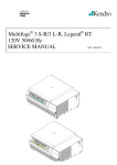
Implementación de un control digital mediante
Linealización Entrada-Salida para un convertidor
conmutado CC-CC elevador (Boost) con filtro de salida.
AUTOR: Lorenzo Pujol.
DIRECTORES: Enrique Cantó, Abdelali El Aroundi.
FECHA: Septiembre 2003.
ÍNDICE GENERAL.
1.- Memoria descriptiva...................................................................................................... 1
1.1.- Introducción.................................................................................................................. 1
1.2.- Objetivos....................................................................................................................... 2
1.3.- Fundamentos teóricos de los convertidores conmutados DC/DC................................ 3
1.4.- Topologías básicas de los convertidores conmutados DC/DC..................................... 3
1.4.1.- Convertidor Buck o reductor.................................................................................... 3
1.4.1.1.- Funcionamiento del convertidor Buck o reductor............................................... 3
1.4.1.1.1.- Topología “ON” del convertidor Buck o reductor......................................... 4
1.4.1.1.2.- Topología “OFF” del convertidor Buck o reductor....................................... 6
1.4.1.2.- Matrices del convertidor Buck o elevador.......................................................... 9
1.4.2.- Convertidor Boost o elevador. ................................................................................ 9
1.4.2.1.- Funcionamiento del convertidor Boost o elevador........................................... 10
1.4.2.1.1.- Topología “ON” del convertidor Boost o elevador..................................... 11
1.4.2.1.2.- Topología “OFF” del convertidor Boost o elevador.................................... 12
1.4.2.2.- Matrices del convertidor Boost o reductor........................................................ 14
1.4.3.- Convertidor Buck-Boost o reductor elevador........................................................ 15
1.4.3.1.- Funcionamiento del convertidor Buck-Boost o reductor-elevador....................16
1.4.3.1.1.- Topología “ON” del convertidor Buck-Boost..............................................16
1.4.3.1.2.- Topología “OFF” del convertidor Buck-Boost.............................................17
1.4.3.2.- Matrices del convertidor Buck-Boost o reductor-elevador................................19
1.4.4.- Convertidor Boost con filtro de salida....................................................................19
1.4.4.1.- Funcionamiento del convertidor Boost con filtro de salida.............................. 21
1.4.4.1.1.- Topología “ON” del convertidor Boost con filtro de salida........................ 22
1.4.4.1.2.- Topología “OFF” del convertidor Boost con filtro de salida....................... 23
1.4.4.2.- Matrices del convertidor Boost con filtro de salida.......................................... 25
1.5.- Control mediante Linealización Entrada-Salida......................................................... 26
1.6.- Simulación mediante Simulink®................................................................................. 30
2.- Memoria de cálculo………………………………………………………………….. 33
2.1.- Introducción................................................................................................................ 33
2.2.- Control mediante Linealización Entrada-Salida......................................................... 33
I
2.3.- Funcionamiento de la planta....................................................................................... 34
2.3.1.- Etapa de potencia................................................................................................... 34
2.3.1.1.- Calculo de las bobinas...................................................................................... 36
2.3.2.- Etapa de control..................................................................................................... 38
2.3.2.1.- Adaptación de la tensión de salida.................................................................... 38
2.3.2.2.- Adaptación de las intensidades de las bobinas.................................................. 41
2.3.2.3.- Filtro Anti-Aliasing........................................................................................... 46
2.3.2.4.- Generación del ciclo de trabajo......................................................................... 49
2.3.2.5.- Alimentación de la placa de control.................................................................. 52
2.3.2.6.- Conversión A/D................................................................................................ 53
2.3.2.7.- Control por Linealización Entrada-Salida........................................................ 54
2.4.- Parámetros principales de la planta............................................................................. 60
2.5.- Listado de todos los componentes calculados............................................................. 61
3.- Planos.................................................................................................................................
3.1.- Etapa de potencia............................................................................................. Lámina 1
3.2.- Sensor de corriente 1........................................................................................ Lámina 2
3.3.- Sensor de corriente 2........................................................................................ Lámina 3
3.4.- Sensor de tensión............................................................................................. Lámina 4
3.5.- Filtro Anti-Aliasing.......................................................................................... Lámina 5
3.6.- Driver IR2125.................................................................................................. Lámina 6
3.7.- Fuente de alimentación.................................................................................... Lámina 7
3.8.- Caja etapa de control........................................................................................ Lámina 8
3.9.- Caja etapa de potencia..................................................................................... Lámina 9
4.- Presupuesto................................................................................................................... 72
4.1.- Precios elementales..................................................................................................... 72
4.1.1.- Capitulo 1: Diseño, Simulación e Implementación............................................... 72
4.1.2.- Capítulo 2: Material............................................................................................... 73
4.2.- Anidamientos.............................................................................................................. 75
4.2.1.- Capítulo 1: Diseño, Simulación e Implementación............................................... 75
4.2.2.- Capítulo 2: Material............................................................................................... 76
4.3.- Aplicación de precios................................................................................................. 78
4.3.1.- Capitulo 1: Diseño, Simulación e Implementación............................................... 79
4.1.2.- Capítulo 2: Material............................................................................................... 79
4.4.- Precio de ejecución por material................................................................................. 81
4.5.- Precio de ejecución por contrato................................................................................. 81
II
4.6.- Precio por licitación.................................................................................................... 81
4.7.- Resumen del presupuesto............................................................................................ 81
5.- Pliego de condiciones................................................................................................... 82
5.1.- Disposiciones y abarque del pliego de condiciones.................................................... 82
5.1.1.- Objetivo del pliego................................................................................................. 82
5.1.2.- Descripción general del montaje............................................................................ 83
5.2.- Condiciones de los materiales..................................................................................... 84
5.2.1.- Especificaciones eléctricas..................................................................................... 84
5.2.1.1.- Placas de circuito impreso................................................................................. 84
5.2.1.2.- Conductores eléctricos...................................................................................... 84
5.2.1.3.- Componentes pasivos........................................................................................ 84
5.2.1.4.- Componentes activos........................................................................................ 84
5.2.1.5.- Zócalos torneados tipo D.I.L............................................................................. 85
5.2.1.6.- Reglamento Electrotécnico de Baja Tensión.................................................... 85
5.2.1.7.- Resistencias....................................................................................................... 85
5.2.1.8.- Condensadores.................................................................................................. 86
5.2.1.9.- Circuitos integrados y semiconductores........................................................... 87
5.2.2.- Especificaciones Mecánicas.................................................................................. 88
5.2.3.- Ensayos, verificaciones y ajustes........................................................................... 88
5.3.- Condiciones de ejecución........................................................................................... 88
5.3.1.- Descripción del proceso......................................................................................... 88
5.3.1.1.- Compra y preparación del material................................................................... 88
5.3.1.2.- Construcción de los inductores......................................................................... 89
5.3.1.3.- Fabricación del circuito impreso....................................................................... 89
5.3.2.- Soldadura de los componentes............................................................................... 90
5.3.3.- Preparación de la caja............................................................................................ 90
5.4.- Condiciones facultativas............................................................................................. 90
5.5.- Conclusiones............................................................................................................... 91
6.- Anexos................................................................................................................................
A1.- Resultados experimentales...................................................................................... A1-1
A1.1.- Introducción....................................................................................................... A1-1
A1.2.- Arranque del convertidor a media carga............................................................ A1-1
A1.3.- Arranque del convertidor a plena carga............................................................. A1-3
A1.4.- Rizado de la intensidad...................................................................................... A1-5
A1.5.- Función Tensión corriente................................................................................. A1-5
A1.6.- Perturbaciones de carga..................................................................................... A1-7
A1.7.- Conclusiones...................................................................................................... A1-9
A2.- Código del programa........................................................................................................
III
A3.-Manual de prácticas................................................................................................. A3-1
A3.1.- Utilización del programa Proview32................................................................. A3-1
A3.2.- Utilización del programa ex51......................................................................... A3-10
A3.3.- Descripción de los Jumpers de configuración................................................. A3-13
A3.4.- Situación de los Jumpers de configuración..................................................... A3-15
A3.5.- Realización de un cable de comunicaciones.................................................... A3-21
A4.- Mejora del programa............................................................................................... A4-1
A4.1.- Introducción....................................................................................................... A4-1
A4.2.- Código del programa......................................................................................... A4-1
A4.3.- Diagrama de bloques......................................................................................... A4-4
A5.- Manuales Técnicos...........................................................................................................
A5.1.- Microcontrolador SAB 80C537..................................................................................
A5.2.- OPA TLC227XIN.......................................................................................................
Bibliografía..............................................................................................................................
IV
1.- MEMORIA DESCRIPTIVA.
Control mediante Linealización Entrada-Salida
1.1.- Introducción.
En la actualidad el número de equipos electrónicos que requieren ser alimentados
en una alta gama de tensiones continuas, con potencias cada vez más elevadas, ha
producido mucho interés en investigación y mejora en sistemas de alimentación basados en
convertidores conmutados.
En un convertidor DC/DC, la tensión de entrada en continua es convertida a tensión
de salida con una mayor o menor magnitud, posiblemente con polaridad opuesta, o bien
aislado las referencias de entrada y masa de salida. Usualmente el control requerido, es casi
siempre diseñado para producir una tensión de salida bien regulada, aún en presencia de
variaciones en la tensión de entrada y en la corriente en la carga.
El bloque de control es una parte integral de cualquier sistema de procesado de
potencia. Una eficiencia alta es esencial en cualquier aplicación cuya razón principal es la
de conservación de la energía. La eficiencia de un convertidor, teniendo en cuenta la
potencia de salida POUT y la potencia de entrada PIN , es:
η=
POUT
PIN
(1.1)
El rendimiento es siempre inferior a la unidad, debido a la presencia de pérdidas de
potencia.
Estas últimas se deben a los elementos resistivos y de los elementos capacitivos,
dispositivos magnéticos (inductores), dispositivos semiconductores operando en modo
lineal (amplificadores) y dispositivos semiconductores operando en modo conmutado
(MOSFET, diodos, etc.).
El siguiente proyecto se centra en los sistemas de alimentación conmutados,
realizando el estudio y el montaje de la placa de potencia y de control digital mediante un
microcontrolador de 8 bits, el SAB 80C537, mediante Linealización Entrada-Salida para
un convertidor continua-continua elevador (Boost).
El contenido del proyecto se divide en un estudio inicial sobre el funcionamiento de
las fuentes conmutadas, realizando un estudio de las diferentes topologías de convertidores
básicos existentes, en un segundo apartado se hará el estudio del control a realizar.
Una vez terminado el estudio teórico con un modelo del microcontrolador, se
fijarán los principales parámetros del convertidor y del control, calculando cada
componente, determinando los requisitos mínimos necesarios de cada elemento.
Como finalización, se realizará una contrastación de los datos y resultados
obtenidos del prototipo con los cálculos y simulación realizadas previamente, obteniendo
así una valoración cualitativa del controlador y de la planta.
1
Memoria Descriptiva.
Control mediante Linealización Entrada-Salida
1.2.- Objetivos.
Dado el grado de importancia que representa la estabilidad de la tensión de salida
en los sistemas de alimentación conmutados se centrará el estudio del sistema en el lazo de
control, así como las diferentes variaciones de este.
Por tanto, el objetivo principal del proyecto es la implementación de un controlador
mediante linealización entrada-salida mediante el microcontrolador SAB 80C537, obtenido
mediante la aplicación de técnicas de bloques de un control robusto mediante una
aplicación de MATLAB® llamado SIMULINK®, comprobando que el comportamiento
delante posibles perturbaciones de la carga, variaciones de tensión de alimentación, ruido u
otros, se aproxima al deseado.
También se realizará el estudio y montaje de la planta, un convertidor Boost
elevador con filtro de salida. En esta planta también se realizan las medidas pertinentes
para obtener los resultados prácticos, y así poder comparar los resultados de las
simulaciones y demostrar el correcto funcionamiento del controlador.
2
Memoria Descriptiva.
Control mediante Linealización Entrada-Salida
1.3.- Fundamentos teóricos de los convertidores conmutados DC/DC.
El funcionamiento básico de un convertidor conmutado DC/DC, consiste en la toma
a diferentes intervalos de la señal continua, ya sea tensión o corriente, una vez eliminado el
ruido y la componente alterna se tendrá que generar un ciclo de trabajo de la señal que
cambia el interruptor.
Para su realización existe un principio de funcionamiento común en todos los tipos
de convertidores conmutados. Este principio consiste en el almacenamiento temporal de
energía y una cesión de esta en un segundo periodo de tiempo, donde su duración
condiciona la cantidad de energía almacenada o cedida, hecho que provoca un mayor o
menor suministro de esta energía a la carga.
1.4.- Topologías básicas de los convertidores conmutados DC/DC.
1.4.1.- Convertidor Buck o reductor.
El convertidor Buck es una fuente conmutada DC-DC que reduce la tensión de
salida con respecto a la tensión de la fuente de alimentación, manteniendo la tensión de
salida constante frente a las variaciones de tensión de la fuente de alimentación o a
variaciones producidas por la carga mediante alguna ley de control, ya sea por corriente,
tensión o corriente y tensión.
El convertidor reductor al tener dos elementos almacenadores de energía, se
encuentra dentro de la familia de los convertidores de segundo orden, ya que no se le ha
agregado ningún filtro a la salida. Este filtro eliminaría el rizado de corriente y tensión,
producido por las diferentes conmutaciones del interruptor. El filtro estaría formado por
una bobina que eliminaría el rizado de corriente y un condensador que eliminaría el rizado
de tensión.
Figura 1.1. Esquema de un convertidor Buck.
Para el análisis se han introducido las resistencias parásitas de la bobina y del
condensador, de esta manera el circuito analizado se acercará más a la realidad.
3
Memoria Descriptiva.
Control mediante Linealización Entrada-Salida
Suponemos para el análisis que cuando el interruptor esta abierto el diodo esta
polarizado en directa, para un periodo de conmutación, y que la corriente de la bobina es
siempre positiva de manera que el convertidor esté siempre trabajando en modo de
conducción continuo. En el otro periodo de conmutación se supone que el interruptor esta
cerrado y el diodo esta polarizado en inversa, no conduce.
El periodo de conmutación del convertidor es T, el interruptor estará cerrado entre
el tiempo 0 < t < DT y estará abierto entre el tiempo DT < t < T, estos dos tipos de
conmutación se verán variados por la ley de control.
La función de este convertidor es la de mantener la relación Vo = D·Vin.
1.4.1.1.- Funcionamiento del convertidor Buck o reductor.
Para el análisis del convertidor y poder encontrar la tensión de salida en función de
las diferentes intensidades y tensiones, se examina la corriente que pasa por la bobina y la
tensión a través de la misma durante un ciclo de conmutación.
La variación neta de la corriente en la bobina en todo el ciclo debe de ser cero así
como la tensión en el condensador, en régimen permanente.
Figura 1.2. Tensión y corriente en la bobina.
Cuando el interruptor esta cerrado y el diodo polarizado en inversa, la corriente en
la bobina aumenta linealmente así como la tensión en el condensador almacenando
energía, cedida de la fuente de alimentación, para luego devolverla a la carga. También en
este periodo se va cediendo energía a la carga.
4
Memoria Descriptiva.
Control mediante Linealización Entrada-Salida
Cuando el interruptor esta abierto y el diodo polarizado en directa , la fuente de
alimentación no cede energía al circuito, es ahora cuando la bobina y el condensador se
comportan como fuentes suministrando energía a la carga. La intensidad y la tensión van
disminuyendo.
1.4.1.1.1.- Topología “ON” del convertidor Buck o reductor.
Figura 1.3. Convertidor Buck en topología “ON”.
Cuando el interruptor está cerrado la fuente de alimentación suministra corriente al
inductor y al resto del circuito, como la tensión de salida Vo es menor que la tensión de
entrada Vin, la corriente que pasa por la bobina será creciente mientras el interruptor este
cerrado, toda esta corriente también pasa por el interruptor y la suministra la fuente de
alimentación.
En todo el ciclo el interruptor se encuentra cerrado y el diodo polarizado en inversa,
cerrado.
Este estado permanecerá durante el tiempo 0 < t < DT, donde T es el periodo de
conmutación y D es el ciclo de trabajo, también llamado factor de servicio.
Este estado se define mediante la ecuación del bucle exterior:
L·
di L
+ io ·R + i L ·RL1 = Vin
dt
(1.2)
Según la ley de tensiones de Kirchoff:
i o = i L − iC = i L − C ·
dVC
dt
(1.3)
5
Memoria Descriptiva.
Control mediante Linealización Entrada-Salida
La ecuación del bucle interior izquierdo se define:
L·
di L
+ iC ·RC1 + i L ·RL1 + VC = Vin
dt
(1.4)
De donde obtenemos la relación:
iC = C ·
dVC
di
1 

=
Vin − L L − i L ·RL1 − VC 
dt
RC1 
dt

(1.5)
Combinando las ecuaciones (1.2) y (1.5) obtenemos:
L·

R·RC
di L
= − RL1 +
dt
R + RC

 R

·i L − 
 R + RC


·VC + Vin (1.6)

La ecuación del bucle interior izquierdo se define:
− VC − iC ·RC + io ·R = 0
(1.7)
Combinando las ecuaciones (1.3) y (1.7) obtenemos:
C·
dVC  RC
= 
dt
 R + RC
 1

·i L − 
 R + RC


·VC

(1.8)
Resolviendo el sistema con las ecuaciones:

R·RC  i L  R
di L
· − 
= − RL1 +
+
dt
R
R
C  L

 R + RC
dVC  RC  i L  1  VC
· − 
·
= 
+
+
dt
R
R
C
R
R
C
C



 C
 VC Vin
· +
L
 L
(1.6) y (1.8)
6
Memoria Descriptiva.
Control mediante Linealización Entrada-Salida
1.4.1.1.2.- Topología “OFF” del convertidor Buck o reductor.
Figura 1.4. Convertidor Buck en topología “OFF”.
Una vez que ha transcurrido el tiempo DT, el interruptor pasa a estar abierto y el
diodo polarizado en directa, dejando pasar corriente. En este periodo es la bobina la que se
comporta como una fuente de alimentación suministrando corriente a la carga, decreciendo
la corriente en la bobina de forma lineal mientras el interruptor permanezca abierto ya que
la derivada de la corriente en la bobina es negativa.
Para que la variación de corriente en la bobina sea nula en régimen permanente,
tiene que ser la misma corriente al principio y al final de cada ciclo de conmutación, por lo
que el periodo debe ser siempre el mismo.
Este intervalo estará comprendido entre DT < t < T.
Este estado se define mediante la ecuación del bucle exterior:
L·
di L
+ io ·R + i L ·RL1 = Vin
dt
(1.9)
Según la ley de tensiones de Kirchoff:
i o = i L − iC = i L − C ·
dVC
dt
(1.10)
La ecuación del bucle interior izquierdo se define:
L·
di L
+ iC ·RC1 + i L ·RL1 + VC = 0
dt
(1.11)
7
Memoria Descriptiva.
Control mediante Linealización Entrada-Salida
De donde obtenemos la relación:
iC = C ·
dVC
− 1  di L

=
+ i L ·RL1 + VC 
L
dt
RC1  dt

(1.12)
Combinando las ecuaciones (1.9) y (1.12) obtenemos:
L·
 R

R·RC 
di L
·i L − 
= − RL1 +
dt
R + RC 
 R + RC


·VC

(1.13)
La ecuación del bucle interior izquierdo se define:
− VC − iC ·RC + io ·R = 0
(1.14)
Combinando las ecuaciones (1.10) y (1.14) obtenemos:
C·
dVC  RC
= 
dt
 R + RC
 1

·i L − 
 R + RC


·VC

(1.15)
Resolviendo el sistema con las ecuaciones:

R·RC  i L  R
di L
· − 
= − RL1 +
dt
R + RC  L  R + RC

dVC  RC  i L  1  VC
· − 
·
= 
dt
 R + RC  C  R + RC  C
 VC
·
 L
(1.13) y (1.15)
8
Memoria Descriptiva.
Control mediante Linealización Entrada-Salida
1.4.1.2.- Matrices del convertidor Buck o elevador.
A partir de las ecuaciones diferenciales (1.6) y (1.8) obtenemos la matriz de la
topología “ON” siguiente:
 di L  −  R + R·RC · 1 −  R · 1  i 
Vin 
 R+ R  L L
 dt    L1 R + R  L
  + 
C 
C 




=
·


L  (1.16)


 1  1 
 dVC    RC · 1
0




−
·
V



 +R  C  C
 dt    R + R  C
123

C 

14444C4442444R4
444
3
B
A
A partir de las ecuaciones diferenciales (1.13) y (1.15) obtenemos la matriz de la
topología “OFF” siguiente:
 di L  −  R + R·RC · 1 −  R · 1  i 
R+R  L  L
 dt    L1 R + R  L
C 
C 


·  + 0

=


0 
 1  VC   
 dVC    RC · i L
{
·  VC 
− 
 dt    R + R  C
R + RC  C 
B
14444C4 442444
44443
A
(1.17)
1.4.2.- Convertidor Boost o elevador.
El convertidor Boost es un tipo de fuente conmutada DC-DC que eleva la tensión
de salida con respecto a la tensión de la fuente de alimentación, manteniéndola constante
frente a variaciones de tensión de la fuente de alimentación o de la carga mediante una ley
de control.
Este convertidor forma parte de los convertidores de segundo orden ya que contiene
dos elementos almacenadores de energía.
Figura 1.5. Esquema de un convertidor Boost.
9
Memoria Descriptiva.
Control mediante Linealización Entrada-Salida
Para una mejor aproximación al convertidor Boost real se han introducido las
resistencias parásitas del condensador y de la bobina. Para el análisis se supone que cuando
el interruptor está cerrado el diodo está polarizado en inversa ya a la inversa. Se supone
también que la tensión en la bobina siempre es positiva.
Cuando el interruptor pase de un estado a otro al no poder la intensidad que pasa
por la bobina cambiar bruscamente se elevará la tensión en la bobina y se sumará a la
tensión de la fuente de alimentación por lo que la tensión de salida se vera aumentada en
respecto a la tensión de entrada.
La función de este convertidor es mantener la relación Vo =
Vin
.
1− D
1.4.2.1.- Funcionamiento del convertidor Boost o elevador.
Para el análisis del convertidor tenemos que observar la corriente en la bobina y la
tensión en el condensador cuando el interruptor está abierto o cerrado, la variación de la
corriente en la bobina en todo el estado debe de ser cero en régimen permanente igual que
la tensión media en bornes de la bobina.
Figura 1.6. Intensidades y tensiones en el Boost.
10
Memoria Descriptiva.
Control mediante Linealización Entrada-Salida
Cuando el interruptor esta cerrado el diodo está polarizado en inversa, la corriente
en la bobina aumenta linealmente, almacenando energía sin transferirla a la carga, mientras
el condensador se comporta como una fuente de alimentación cediendo energía a la carga.
Cuando el interruptor esta abierto y el diodo está polarizado en directa es la bobina
la que se comporta ahora como una fuente de alimentación, cediendo energía al
condensador y a la carga, el condensador se comporta ahora como carga, almacenando
energía para el próximo periodo de conmutación, en este periodo la corriente de la bobina
va disminuyendo linealmente cediéndose a la carga. En este cambio la tensión que se
genera en la bobina se suma a la tensión de la fuente de alimentación ya que tiene la misma
polaridad.
1.4.2.1.1.- Topología “ON” del convertidor Boost o elevador.
Figura 1.7. Convertidor Boost en topología “ON”.
Cuando el interruptor esta cerrado y el diodo polarizado en inversa, la fuente de
alimentación suministra corriente a la bobina, almacenándola, mientras el condensador se
comporta como una fuente alimentando a la carga. Este sistema estará comprendido entre
0 < t < DT.
La corriente que pasará por el diodo será prácticamente nula. La bobina se
comportará como receptor y el condensador como fuente.
El sistema de ecuaciones del bucle izquierdo se define:
L·
di L
+ i L ·RL1 = Vin
dt
(1.18)
Según la ley de tensiones de Kirchoff:
i o = iC = C ·
dVC
dt
(1.19)
11
Memoria Descriptiva.
Control mediante Linealización Entrada-Salida
La ecuación del bucle derecho se define:
dVC  1 
·VC = 0
+
dt  R + RC 
Resolviendo el sistema con las ecuaciones:
C·
(1.20)
di L
i
Vin
= −(RL1 )· L +
dt
L
L
 1  VC
dVC
·
= −
dt
R
+
R
C  C

(1.18) y (1.20)
1.4.2.1.2.- Topología “OFF” del convertidor Boost o elevador.
Figura 1.8. Convertidor Boost topología “OFF”.
Una vez transcurrido el tiempo DT el interruptor pasa a estar cerrado y el diodo a
estar polarizado en directa, actuando ahora la bobina como un generador de corriente,
alimentando a la carga y al condensador, este almacena energía para el próximo subintervalo.
La tensión de la bobina se suma a la tensión de la fuente de alimentación y el
condensador se carga a esta tensión elevando de esta forma la tensión de salida.
Este estado durará mientras el interruptor este cerrado en DT < t < T..
12
Memoria Descriptiva.
Control mediante Linealización Entrada-Salida
Este estado se define mediante la ecuación del bucle exterior:
di L
+ io ·R + i L ·RL1 = Vin
dt
Según la ley de tensiones de Kirchoff:
L·
i o = i L − iC = i L − C ·
dVC
dt
(1.21)
(1.22)
La ecuación del bucle interior izquierdo se define por:
L·
di L
+ iC ·RC1 + i L ·RL1 + VC = Vin
dt
(1.23)
De donde obtenemos la relación:
iC = C ·
dVC
di
1 

=
Vin − L L − i L ·RL1 − VC 
dt
RC1 
dt

(1.24)
Combinando las ecuaciones (1.21) y (1.24) obtenemos:
L·
 R

R·RC 
di L
·i L − 
= − RL1 +
dt
R + RC 
 R + RC


·VC + Vin (1.25)

La ecuación del bucle interior izquierdo se define:
− VC − iC ·RC + io ·R = 0
(1.26)
Combinando las ecuaciones (1.22) y (1.26) obtenemos:
C·
dVC  RC
= 
dt
 R + RC
 1

·i L − 
 R + RC


·VC

(1.27)
Resolviendo el sistema con las ecuaciones:

R·RC  i L  R
di L
· − 
= − RL1 +
dt
R + RC  L  R + RC

dVC  RC  i L  1  VC
· − 
·
= 
dt
R
+
R
C
R
+
R
C 
C  C


 VC Vin
· +
L
 L
(1.25) y (1.27)
13
Memoria Descriptiva.
Control mediante Linealización Entrada-Salida
1.4.2.2.- Matrices del convertidor Boost o reductor.
A partir de las ecuaciones diferenciales (1.18) y (1.20) obtenemos la matriz de la
topología “ON” siguiente:
 di L  −  R + R·RC · 1 −  R · 1  i 
Vin 
 R+ R  L L
 dt    L1 R + R  L
  + 
C 
C 




=
·


L  (1.28)


 1  1 
 dVC    RC · 1
0




−
·
V



 +R  C  C
 dt    R + R  C
123

C 
14444C4442444R4

444
3
B
A
A partir de las ecuaciones diferenciales (1.25) y (1.27) obtenemos la matriz de la
topología “OFF” siguiente:
 di L  −  R + R·RC · 1 −  R · 1  i 
 R+ R  L L
 dt    L1 R + R  L
C 
C 



· 
=



 RC  1
 1  1 
 dVC 

·

·  V 
−

 dt  
R + RC  C   C 
+ RC  C

144R4
444424444444
3
A
Vin 
+  L 


0 
12
3
B
(1.29)
14
Memoria Descriptiva.
Control mediante Linealización Entrada-Salida
1.4.3.- Convertidor Buck-Boost o reductor elevador.
Este tipo de fuente conmutada permite elevar o disminuir la tensión de salida en
respecto a la tensión de entrada según sea su ciclo de trabajo. También forma parte de los
convertidores de segundo orden ya que solo tiene dos elementos almacenadores de energía.
Este convertidor invierte la tensión de salida con respecto a la tensión de la fuente
de alimentación.
Este convertidor se comporta como los convertidores ya mencionados
anteriormente, se comporta como si el convertidor Buck y Boost se encontraran en
cascada.
Figura 1.9. Esquema de un convertidor Buck-Boost.
 D 
La función de este convertidor es la de mantener la relación Vo = −Vin
 . Si
1− D 
el ciclo de trabajo es D < 1 2 el convertidor se comporta como un Buck, reduciendo la
tensión de salida con respecto a la de entrada. Si el ciclo de trabajo es D > 1 2 el
convertidor se comporta como un Boost, elevando la tensión con respecto a la tensión de
entrada.
15
Memoria Descriptiva.
Control mediante Linealización Entrada-Salida
1.4.3.1.- Funcionamiento del convertidor Buck-Boost o reductor-elevador.
Para el análisis de este convertidor es examinar la tensión en el condensador y la
corriente en la bobina es los diferentes estados en que se encuentra el interruptor. La
variación de corriente y tensión en la bobina en régimen permanente debe de ser cero.
Figura 1.10. Intensidad en la bobina.
Cuando el interruptor está cerrado el diodo se polariza en inversa, no deja pasar
corriente, la corriente en la bobina aumenta linealmente almacenando energía para el
próximo periodo de conmutación, mientras el condensador se comporta como una fuente
suministrando energía a la carga.
Cuando el interruptor está abierto al no poder cambiar bruscamente la corriente que
pasa por la bobina y el diodo se polariza en directa, pasando corriente hacia la carga, en
este periodo el condensador almacena energía para luego devolverla a la carga en el
próximo periodo de conmutación.
1.4.3.1.1.- Topología “ON” del convertidor Buck-Boost.
Figura 1.11. Convertidor Buck-Boost en topología “ON”.
16
Memoria Descriptiva.
Control mediante Linealización Entrada-Salida
Cuando el interruptor está cerrado y el diodo polarizado en inversa, la fuente de
alimentación suministra corriente a la bobina aumentando esta linealmente, en este estado
la bobina almacena energía, mientras el condensador suministra energía a la carga
comportándose como una fuente, la tensión en el condensador va disminuyendo. Este
periodo está comprendido entre 0 < t < DT.
Este estado se define mediante las ecuaciones del bucle izquierdo:
L·
di L
+ i L ·RL1 = Vin
dt
(1.30)
Según la ley de tensiones de Kirchoff:
i o = iC = C ·
dVC
dt
(1.31)
La ecuación del bucle derecho se define:
C·
dVC  1
+
dt  R + RC

·VC = 0

(1.32)
Resolviendo el sistema modificando las ecuaciones:
di L
i
Vin
= −(RL1 )· L +
dt
L
L
 1  VC
dVC
·
= −
dt
R
R
+
C
 C

(1.30) y (1.32)
1.4.3.1.2.- Topología “OFF” del convertidor Buck-Boost.
Figura 1.12. Convertidor Buck-Boost en topología “OFF”.
17
Memoria Descriptiva.
Control mediante Linealización Entrada-Salida
Una vez transcurrido el tiempo DT el interruptor pasa a estar abierto y el diodo
polarizado en directa, en este periodo la bobina se comporta como una fuente de
alimentación que cede energía a la carga y al condensador. Debido a que la corriente que
pasa por la bobina debe de tener continuidad el condensador provoca una tensión en
inversa por lo que la tensión en la salida estará invertida con respecto a la tensión de
entrada.
Permanecerá en este intervalo mientras se cumpla DT < t < T.
Las ecuaciones del bucle exterior vienen definidas por:
L·
di L
+ io ·R + i L ·RL1 = Vin
dt
(1.33)
Según la ley de tensiones de Kirchoff:
i o = i L − iC = i L − C ·
dVC
dt
(1.34)
La ecuación del bucle interior izquierdo se define:
L·
di L
+ iC ·RC1 + i L ·RL1 + VC = 0
dt
(1.35)
De donde obtenemos la relación:
iC = C ·
dVC
di
1 

=
 − L L − i L ·RL1 − VC 
dt
RC1 
dt

(1.36)
Combinando las ecuaciones (1.34) y (1.36) obtenemos:
L·
 R

R·RC 
di L
·i L − 
= − RL1 +
dt
R + RC 
 R + RC


·VC

(1.37)
La ecuación del bucle interior derecho se define:
− VC − iC ·RC + io ·R = 0
(1.38)
Combinando las ecuaciones (1.34) y (1.38) obtenemos:
C·
dVC  RC
= 
dt
 R + RC
 1

·i L − 
 R + RC


·VC

(1.39)
18
Memoria Descriptiva.
Control mediante Linealización Entrada-Salida
Resolviendo el sistema con las ecuaciones:

R·RC  i L  R
di L
· − 
= − RL1 +
dt
R + RC  L  R + RC

dVC  RC  i L  1  VC
· − 
·
= 
dt
 R + RC  C  R + RC  C
 VC
·
 L
(1.37) y (1.39)
1.4.3.2.- Matrices del convertidor Buck-Boost o reductor-elevador.
A partir de las ecuaciones diferenciales (1.30) y (1.32) obtenemos la matriz de la
topología “ON” siguiente:
 i
 di L   RL1
0
Vin 
L 
 dt  − L





=

 1  1 ·  +  L  (1.40)
 dVC   0
·
− 
0 
 
12
 dt  
R + RC  C  VC 
3

14444244443
B
A
A partir de las ecuaciones diferenciales (1.37) y (1.39) obtenemos la matriz de la
topología “OFF” siguiente:
 di L  −  R + R·RC · 1 −  R · 1  i 
 R+ R  L L
 dt    L1 R + R  L
C 
C 


·  + 0

=


0 
 1  1 
 dVC    RC · 1
{
·  VC 
− 
 dt    R + R  C
+ RC  C 
B
 4444C4442444R4
1
444
3
A
(1.41)
1.4.4.- Convertidor Boost con filtro de salida.
Este convertidor es del tipo elevador, pero gracias al filtro de salida formado por
una bobina y un condensador, el rizado de corriente y de tensión, producido por las
diferentes conmutaciones del interruptor se ve disminuido en función del tamaño de la
bobina y del condensador de salida.
Este convertidor forma parte de los convertidores de cuarto orden al estar
constituido por cuatro elementos almacenadores de energía.
19
Memoria Descriptiva.
Control mediante Linealización Entrada-Salida
Figura 1.13. Esquema de un convertidor Boost con filtro de salida.
Para una mejor aproximación a la realidad se han introducido las resistencias
parásitas de los cuatro elementos almacenadores de energía.
La función de este convertidor es mantener la relación Vo =
Vin
.
1− D
Siendo D el factor de servicio del controlador en régimen estacinario.
20
Memoria Descriptiva.
Control mediante Linealización Entrada-Salida
1.4.4.1.- Funcionamiento del convertidor Boost con filtro de salida.
Para el análisis de este convertidor se deben de encontrar las intensidades que pasan
por las dos bobinas y las tensiones que hay en los dos condensadores en los dos ciclos de
trabajo del interruptor.
Figura 1.14. Tensión en la bobina 1 y corriente en las bobinas.
Cuando el interruptor está cerrado el diodo se polariza en inversa, no deja pasar
corriente. La bobina 1 queda en bornes de la fuente de alimentación cargándose
linealmente de corriente, mientras los condensadores y la bobina ceden energía a la carga,
sin invertir la polaridad de la tensión en la carga, se van descargado en la carga.
Cuando el interruptor esta abierto, el diodo se polariza en directa, deja pasar
corriente, es cuando la bobina 1 cede energía almacenada a los demás elementos
almacenadores de energía y a la carga, sumando la tensión que hay en la bobina a la de la
fuente, de esta manera la tensión en la salida se ve aumentada con respecto a la tensión de
salida.
El filtro de salida elimina las componentes de alta frecuencia, eliminando el rizado
de la corriente, que se encargaría la bobina 2, y de tensión, que se encargaría el
condensador 2.
21
Memoria Descriptiva.
Control mediante Linealización Entrada-Salida
1.4.4.1.1.- Topología “ON” del convertidor Boost con filtro de salida.
Figura 1.15. Convertidor Boost con filtro de salida en topología “ON”.
Cuando el interruptor está cerrado la bobina 1 queda en bornes de la fuente de
alimentación almacenando energía, la corriente que va a la bobina 1 crece linealmente. El
diodo al estar polarizado en inversa no deja pasar corriente, y los demás elementos
almacenadores de energía van cediendo parte de su energía a la carga. La bobina 1 y el
condensador 2 filtran la corriente y la tensión eliminando el rizado en la carga.
Este estado se comprende entre 0 < t < DT.
Para el análisis del convertidor se deben de encontrar las tensiones que hay en los
dos condensadores y las corrientes que pasan por las bobinas.
La ecuación del bucle izquierdo:
L1 ·
di L1
+ i L1 ·RL1 = Vin
dt
(1.42)
La ecuación del bucle interior derecho:
iL 2 = −C1 ·
dVC1
dt
(1.43)
La ecuación del bucle exterior derecho se define:
L2 ·
R·RC 2
di L 2
R
+ i L 2 ·RC 2 + i L 2 ·RC1 +
·i L 2 +
·VC 2 = VC1
dt
R + RC 2
R + RC 2
(1.44)
La ecuación del bucle interior derecho se define:
22
Memoria Descriptiva.
Control mediante Linealización Entrada-Salida
dVC 2
dt
+ io ·R = 0
i o = i L 2 − iC 2 = i L 2 − C 2 ·
(1.45)
− VC 2 − iC 2 ·RC 2
(1.46)
Combinando la ecuación (1.44) y (1.45) obtenemos:
C2 ·
dVC 2  RC
= 
dt
 R + RC 2


1
·i L 2 − 

 R + RC 2

·VC 2

(1.47)
Resolviendo el sistema con las siguientes ecuaciones:
di L1
R
Vin
= − L1 ·i L1 +
dt
L1
L1
dV C 1 − i L 2
=
dt
C1

R·RC 2
di L 2
= − RC 2 + RC 1 +
dt
R + RC 2

dV C 2  RC 2
= 
dt
 R + RC 2
 iL 2 
R
·
− 
 L 2  R + RC 2
 iL 2 
1
·
− 
 C 2  R + RC 2
 VC 2 VC 1
· L + L
2
 2
(1.42) (1.43)
(1.44) (1.47)
 VC 2
·
 C2
1.4.4.1.2.- Topología “OFF” del convertidor Boost con filtro de salida.
Figura 1.16. Convertidor Boost con filtro de salida en topología “OFF”.
Cuando el interruptor está cerrado el diodo se polariza en directa. La bobina 1 se
comporta como una fuente cediendo su energía almacenada a los otros elementos
almacenadores de energía, estos eliminan el rizado de la corriente y de la tensión
suministrando energía a la carga.
En este estado de corriente de la bobina 1 va decreciendo linealmente mientras que
en la bobina 2 va aumentando, también aumenta la tensión en los dos condensadores.
23
Memoria Descriptiva.
Control mediante Linealización Entrada-Salida
La tensión en la carga es la suma de la tensión de la fuente de alimentación y de la
bobina 1, de esta manera la tensión en la salida siempre es mayor que la tensión de entrada.
Este estado está comprendido entre DT < t < T.
Las ecuaciones del bucle izquierdo:
dVC1
= iC1 = i L1 − i L 2
dt
(1.48)
di L1
+ i L1 ·R L1 + i L1 ·RC1 − i L 2 ·RC1 + VC1 = Vin
dt
(1.49)
C1 ·
L1 ·
La ecuación del bucle exterior derecho:
L2 ·
R· RC 2
di L 2
R
+ i L1 ·R L1 +
·i L 2 + i L 2 ·RC1 − i L1 ·RC1 +
·VC 2 = VC1
dt
R + RC 2
R + RC 2
(1.50)
Las ecuaciones del bucle interior derecho se define:
i o = i L 2 − iC 2 = i L 2 − C 2 ·
dVC 2
dt
− VC 2 − iC 2 ·RC 2 + io ·R = 0
(1.51)
(1.52)
Combinando la ecuación (1.51) y (1.52) obtenemos:
C2 ·
dVC 2  RC
= 
dt
 R + RC 2


1
·i L 2 − 
 R + RC 2


·VC 2

(1.53)
Resolviendo el sistema con las siguientes ecuaciones:
V
R
Vin
i
di L1
= − (RL1 + RC 1 )· L1 + C 1 ·iL 2 − C 1 +
L1
L1
L1
L1
dt
dVC 1 iL1 iL 2
=
−
dt
C1 C1

V
R ·RC 2  iL 2  R  VC 2 RC 1
di L 2
·
· − 
·iL1 + C 1
+
= − RC 2 + RC 1 +
L2
R + RC 2  L2  R + RC 2  L2
L2
dt

(1.49) (1.48)
(1.50) (1.53)
 VC 2
dVC 2  RC 2  iL 2 
1
·
· − 
= 
dt
 R + RC 2  C 2  R + RC 2  C 2
24
Memoria Descriptiva.
Control mediante Linealización Entrada-Salida
1.4.4.2.- Matrices del convertidor Boost con filtro de salida.
A partir de las ecuaciones diferenciales (1.42) (1.43) (1.44) y (1.47) obtenemos la
matriz de la topología “ON” siguiente:
 i 
 di L1  − R L1 0
0
0
  L1 
 dt   L1
   Vin 

 
1

 V   L 
dV
 C1 
0
0
0
−

  C1   1 
C
 dt 
1

=

 R  1 ·  +  0 
R·RC 2  1
1
·
·
 di L 2   0
−  RC 2 + RC1 +
− 
i   0 

L2
R + RC 2  L 2
 dt  

 R + RC 2  L 2   L 2  



0 
 dV 

 1    12
 RC 2  1
1
3
C
2

·

·


0
0
− 
V 
B
R + RC 2  C 2
RC 2  C 2   C 2 
 dt  
 R4+4
1444444444444
24444444
444
3
A
(1.54)
A partir de las ecuaciones diferenciales (1.49) (1.48) (1.50) y (1.53) obtenemos la
matriz de la topología “OFF” siguiente:
RC 1
 i 
 di L1  − (R + R )· 1 − 1
0
L1
C1

  L1 
 dt 
L1
L1
L1
 

 
1
1

 V 
dV
 C1 
−
0
0
  C1 
C1
C1
 dt  


=

 R  1  · 
RC 1
R·RC 2  1
1
·
·
 di L 2  
−  RC 2 + RC1 +
− 
i 
L2
L2
R + RC 2  L 2
 dt  

 R + RC 2  L 2   L 2 

 dV  
 RC 2  1

 1  
1




 C2  
−
0
0
·
 
 R + R · C
R + RC 2  C 2  VC 2 
 dt  
C2 
2


1444444444444442444444444444443
B
Vin 
L 
 1
+ 0 


 0 
 0 
123
B
(1.55)
25
Memoria Descriptiva.
Control mediante Linealización Entrada-Salida
1.5.- Control mediante Linealización Entrada-Salida.
En el modo de conducción continua, un convertidor conmutado puede representarse
mediante dos ecuaciones diferenciales vectoriales lineales a tramos como sigue:
.
x = A1 · x + B1 para 0 ≤ t ≤ TON
.
x = A2 · x + B2 para TON ≤ t ≤ T
(1.56)
(1.57)
Donde x es el vector de estado y T es el periodo de conmutación.
La resolución a tramos de las ecuaciones de estado y la posterior combinación de
las mismas dan lugar a la expresión:
x(T ) = H · x(0) + F ·x(0)·τ (0) + g ·τ (0) + k
(1.58)
Donde aparece el vector de estado al final de un intervalo de conmutación
cualquiera en función de las variables de estado y el control al principio del intervalo. Si la
frecuencia de conmutación es suficientemente elevada respecto a las frecuencias propias
del sistema podemos escribir que:
H = e A2 ·T
F = H ·( A1 − A2 )
g = H ·( B1 − B2 )·Vin k = H · A2−1 ·( I − e − A2 ·T )·B2 ·Vin
(1.59)
Para el convertidor Boost de la siguiente figura:
Figura 1.17. Convertidor Boost con filtro de salida.
26
Memoria Descriptiva.
Control mediante Linealización Entrada-Salida
Las matrices de (1.56) y (1.57) son:

0

0
A1 = 

0

0

−1
den
0
L1
den
0
−

0
1

C
A2 =  1

0

0

1 
den 

0 

− L1 

den 
−1 
R·C 2 
0
1
C1
0
1
C2
 L2 
 den 


B1 = B 2 =  −01 


 den 
 0 
− L2
den
0
L1
den
0
0
−
1
C1
0
1
C2
1 
den 

0 

− L1 

den 
−1 
R·C 2 
(1.60)
 il1 
 Vc1 

x=
 il 2 


Vc 2
den = L1 ·L 2
Si consideramos el caso más sencillo sin acoplo magnético ( M = 0 ) las ecuaciones
siguientes se pueden escribir como:

1

T
C
H = 1
0


0

−T
L1
1
T
L2
0
0
−
T
C1
1
T
C2




0

−T 

L2 
T 
1+
R·C 2 
0
 T

 L

1


2
 T  
k = 
·Vin
L1 ·C1  



 0 
 0 
 T 

 
  L1 ·C1 
 −1
F =  C1

 − T 


L
C
·
2
1



0


1
0 0
L1


 T 

 0 0 
 L1 ·C1 


0
0 0

0
0 0 
(1.61)
0 
0 
g= 
0 
 
0 
27
Memoria Descriptiva.
Control mediante Linealización Entrada-Salida
A partir de la expresión (1.58) podemos obtener varias expresiones de τ(0) para el
convertidor Boost, una por cada variable de estado como puede verse a continuación:
4
τ (0) =
xi (T ) − ∑ hij · x j (0) − k i
j =1
4
∑f
j =1
ij
(1.62)
·x j (0) + g i
Donde i = 1...4.
Si intentamos conseguir que entre una variable y su consigna se reduzca de forma
exponencial ( ciclo a ciclo ) de la forma:
xi (T ) − xi* = W ( xi (0) − xi* )
(1.63)
Podemos rescribir la ecuación (1.60) como:
4
τ (0) =
W ·xi (0) + (1 − W )·xi* − ∑ hij ·x j (0) − k i
j =1
4
∑f
j =1
ij
(1.64)
·x j (0) + g i
La expresión anterior cuando la variable a linealizar es la tensión de salida (i = 4)
presenta un denominador nulo por lo cual deducimos que no es posible controlar el
convertidor en este caso.
Si tomamos la tensión intermedia Vc1 como variable a linealizar, obtenemos la
siguiente expresión del ciclo de trabajo.
[
C
− T ·Vin
− il1 + il 2 + 1 [W − 1]· Vc1 − Vc1*
L1
T
τ
=
T
T
− il1 + ·Vc1
L1
]
(1.65)
En las matrices de la ecuación (1.61) se puede observar algunos términos entre
paréntesis, son los términos de segundo orden, condensador y bobina, que no han sido
eliminador junto con los términos en τ2.
Eliminándolos y recalculando el ciclo de trabajo obtenemos:
τ
T
=
− il1 + il 2 +
[
C1
[W − 1]· Vc1 − Vc1*
T
− il1
]
(1.66)
28
Memoria Descriptiva.
Control mediante Linealización Entrada-Salida
La sustitución de la ecuación anterior en el sistema de ecuaciones promediado, se
obtiene:
.
τ
τ
 τ
x = ( A1 ·x + B1 ·Vin )· + ( A2 ·x + B2 ·Vin )·1 −  = ( A2 ·x + B2 ·Vin ) + ( A1 − A2 )·
T
T
 T
(1.67)
Donde B1 = B2 , nos proporciona las siguientes ecuaciones:
L1 ·
(
i ·V
V
di L1
= Vin − L 2 C 1 + k · C 1 VC 1 − VC*1
dt
i L1
i L1
(
dVC 1
= − k · VC 1 − VC*1
dt
di
L2 · L 2 = VC 1 − VC 2
dt
dV
V
C 2 · C 2 = iL 2 − C 2
dt
R
C1 ·
k=
)
)
(1.68)
C1
[W − 1] < 0
T
29
Memoria Descriptiva.
Control mediante Linealización Entrada-Salida
1.6.- Simulación mediante Simulink®.
Una vez obtenidas las ecuaciones características del convertidor Boost con filtro de
salida se sabe que:
.
x = A1 · x + B1 para t ≤ TON
.
x = A2 · x + B2 para TON ≤ t ≤ T
(1.69)
(1.70)
Si cogemos las ecuaciones A1 y A 2 y las comparamos obtenemos que son
diferentes mientras que las matrices B1 y B 2 son iguales.
La diferencia entre la matriz A2 y la A1 son los siguientes aspectos:
RC1
 i 
diL1  − (R + R )· 1 (1− u) − 1 (1− u)
(1− u)
0
L1
C1

  L1 
 dt 
L1
L1
L1
 

 
1
1
 V 
dVC1  
−
(1− u)
0
0
  C1 
C1
C1
 dt  

=



 R  1 ·  + B2
R·RC2  1
RC1
1
di

L
2


−  RC2 + RC1 +
(1− u)


· L −  R + R · L  iL2 
+
R
R
L2
L2
 dt  
C2  2
C2  2 



 
dV  




R
1
1
1
 C2 ·
·   
 C2  
− 
0
0

 VC2 
+
+
R
R
C
R
R
dt

 
C2  2
C2  C2 
444
1444444444444444424
4444444444
443
A2
(1.80)
La matriz A1 solo tiene un valor diferente que es en la intensidad de la bobina 1:
 i 
 di L1  − R L1 (u ) 0
0
0
  L1 
 dt   L1
 
 

1
dV
 V 

 C1 
0
0
0
−
  C1 

C
 dt 
1
=

 R  1 ·  + B1

R·RC 2  1
1
·
·
 di L 2  
0
− 
−  RC 2 + RC1 +
i 
L2
R + RC 2  L 2
 dt  
 R + RC 2  L 2   L 2 


 dV  
 1  

 RC 2  1
1
2
C

·
·



0
0
− 
 
R + RC 2  C 2
R + RC 2  C 2  VC 2 
 dt  


1444444444444
424444444444444
3
A1
(1.81)
30
Memoria Descriptiva.
Control mediante Linealización Entrada-Salida
Vin 
L 
 1
(1.82)
 0 


 0 
 0 
123
B1 = B2
Una vez encontradas las diferencias entre las matrices solo tenemos que realizar el
diagrama de bloques mediante Simulink®.
Para la obtención de una variable del circuito, como por ejemplo la tensión en el
condensador de salida, que sería la tensión de salida del convertidor Boost con filtro de
salida, será la siguiente:
 dVC 2   RC 2
 dt  =  R + R

 
C2

 1
1
· ·i L 2 − 
 R + RC 2
 C2
 1
· ·VC 2
 C2
(1.83)
Figura 1.18. Simulación de la tensión de salida.
De esta manera se generan unos bloques donde tendremos las tensiones en los
condensadores y las corrientes en las bobinas.
Una vez obtenidas las tensiones y corrientes de nuestro convertidor solo tenemos
que aplicar la formula de Linealización Entrada-Salida.
Ciclo de trabajo =
- IL1 + IL2 - k·(Vo - Vo_deseada )
- IL1
(1.84)
Una vez obtenido el ciclo de trabajo se compara este valor con una señal rampa
entre los valores 0 y 1, esta comparación generará una señal cuadrada que cambiará según
el ciclo de trabajo.
31
Memoria Descriptiva.
Control mediante Linealización Entrada-Salida
Figura 1.19. Simulación del control.
32
Memoria Descriptiva.
2.- MEMORIA DE CÁLCULO.
Control mediante Linealización Entrada-Salida
2.1.- Introducción.
En este capítulo se explicará detalladamente el control mediante Linealización
Entrada-Salida, tanto la parte de hardware como la de software, se justifica los diseños de
los circuitos, así como los materiales utilizados y el algoritmo implementado a la hora de
implementar los diferentes circuitos.
VREF +
Vo
e
−
Linealización
Entrada-Salida
u
Boost
IL1
IL 2
Figura 2.1. Diagrama de bloques del controlador.
Se explicará también los parámetros de la planta así como los componentes de esta,
así como se debe utilizar la placa Altair para el microcontrolador 80C537, así como el
programa utilizado para la programación de este.
2.2.- Control mediante Linealización Entrada-Salida.
Para realizar el control del convertidor Boost se debe de obtener las variables del
convertidor Boost, que en nuestro caso serán la intensidad que pasa por las dos bobinas y
la tensión de la salida del convertidor, estas variables se verán afectadas por las variaciones
de carga y de tensión de entrada.
La implementación de este control por Linealización por Entrada-Salida se ha
realizado con un sistema digital en un microcontrolador 80C537. Se ha escogido un
sistema de control digital para la implementación de este control ya que al tenerse que
realizar multiplicaciones y divisiones sería muy difícil la implementación en analógico.
La elección del microcontrolador 80C537 ha sido de obligada elección ya que
realiza multiplicaciones y divisiones por hardware de una manera rápida y sencilla.
33
Memoria de cálculo
Control mediante Linealización Entrada-Salida
El uso de un microcontrolador provoca la aparición de circuitos adicionales para
poder tratar la señal de forma adecuada. Un diagrama de bloques más detallado para la
realización del control sería el siguiente:
Figura 2.2. Diagrama de bloques del control.
2.3.- Funcionamiento de la planta.
En este apartado se explicará todos los elementos de la planta, tanto la etapa de
potencia como la de control, así como los componentes y porque de su elección.
La tensión de alimentación de la etapa de potencia y de control, así como la placa
del microcontrolador será de 12 V en continua.
2.3.1.- Etapa de potencia.
I1 +
Vin + 12 V
I1 -
1
R24
0.25 6W
I2 +
L1
2
1
0.69m
D3
2
1
R25
Vo
L2
2
0.25 6W
BYW 29
2
I2 -
1.22 m
R26
1
Gate
3
2
10 1/2 W
Q1
BUK 455
1
2
2
C4
1
2
2
2
2
C5
C6
C7
C8
1 22u
1 22u
1 2.2u
1 22u
1n
2
C9
1 100u
2
C10
1 2.2u
2
R28
R27
48 12 W
1
68 12 W
1
Figura 2.3. Etapa de potencia
Para calcular las resistencias en serie con las bobinas así como la potencia que
deben de soportar, se calcula mediante la resistencia de estas así como la intensidad
máxima que puede pasar por estas, que en nuestro caso es de 2.5 A.
P = R·I 2 = 0.25Ω·2.5 2 = 1.56W
(2.1)
Se ha escogido una resistencia de 0.25 Ω y 6 W de potencia ya que el precio para
una resistencia de 2 W era el mismo que una de 6 W. Al tener que introducir la placa
dentro de una caja el rendimiento de disipación de las resistencias se vera afectado por lo
que la potencia que pueden aguantar se tiene que dimensionar con un margen elevado.
El MOSFET de potencia utilizado es el BUK455, este transistor puede soportar
corrientes medias de hasta 26 A, con una resistencia en conducción típica de 0.07 Ω a
34
Memoria de cálculo
Control mediante Linealización Entrada-Salida
temperatura ambiente, pero se ha escogido también ya que el tiempo de pasar de corte a
conducción es del orden de 30 ns.
El diodo rápido de potencia que se ha optado para el circuito es el BYW 29, este
diodo puede soportar corrientes medias de 15 A y soportar tensiones inversas de hasta 200
V, con un tiempo de pasar del estado de conducción al de corte de 25 ns.
Los Condensadores utilizados para el almacenamiento de energía son los
electrolíticos ya que por su reducido tamaño y su gran capacidad de almacenar energía son
los idóneos para la realización del circuito, pero tienen el problema que no son rápidos a la
hora de absorber el rizado de las tensiones, a frecuencias elevadas, por lo que también se
han introducido condensadores cerámicos que estos si que pueden absorber las tensiones
elevadas, a frecuencias elevadas, pero tienen el inconveniente que ocupan mucho espacio y
los valores de capacidad son muy pequeños.
La protección del MOSFET de potencia se realiza mediante un filtro paso bajos que
elimina las componentes frecuenciales de alta frecuencia que podrían dañar el MOSFET ya
que producen tensiones muy elevadas, también sirve para la eliminación de tensiones
elevadas cuando el MOSFET no esta conduciendo.
2
R26
10 1/2 W
1
2
C4
1
1n
Figura 2.4. Filtro Paso-Bajos .
1
s+
1
RCs + 1
RC
H (s) = R +
=
= R·
Cs
Cs
s
s + 10 8
H ( s ) = 10·
s
(2.2)
(2.3)
La elección de las resistencias de carga se ha realizado para que puedan aguantar
tensiones de 22 V, y se han elegido con una resistencia de 48 Ω y de 68 Ω. La elección de
la potencia se ha calculado mediante las formulas siguientes:
Para la resistencia de 48 Ω:
U 2 22 2
P=
=
= 10.08 W
R
48
(2.4)
35
Memoria de cálculo
Control mediante Linealización Entrada-Salida
Para la resistencia de 68 Ω:
P=
U 2 22 2
=
= 7.11 W
R
68
(2.5)
En todo caso se han elegido para que puedan soportar 12 W ya que el precio no
tenía casi variación y al tener que introducir la placa dentro de una caja necesitan tener un
margen.
2.3.1.1.- Calculo de las bobinas.
TOROIDAL POLVO DE HIERRO
O-ring iron-dust core
• Material grado 75
NTH 039
∆lµh/100 Turns(vueltas): 1000 ± 10%
Dimensiones en mm. Ø Ext.: 39,80
Dimensiones en mm. Ø Int.: 24,13
Dimensiones en mm. Alto: 14,48
Figura 2.5. Núcleo toroidal de las bobinas.
Se ha escogido un núcleo de polvo de ferrita ( núcleo para la construcción de
inductores de acumulación) ya que es el más indicado para la construcción de bobinas de
almacenamiento de energía, también por la poca variación de ∆L.
Una vez escogido el núcleo es el momento de la elección del tamaño de este. Según
las vueltas de hilo que se tengan que dar al núcleo y según la inductancia que se quiera
llegar se escogerá el núcleo. Para un valor de la bobina de 0.69 mH se escogerá el núcleo
NTH 039 ya que es el que tiene la ∆L más elevada.
Se observa que tiene una inductancia nominal ∆L de 1 mH/100 vueltas ± 10%. Por
tanto la mínima inductancia para este núcleo es de 900 µH/100 vueltas.
Para el cálculo de la bobina 1, de 0.69 mH se utilizará la siguiente fórmula:
L = ∆ L × N 2 × 10 −6
N 1 = 10 3 ×
L
0.00069
= 10 3 ×
= 276.88 ≈ 277vueltas
0.9
∆L
100
(2.6)
(2.7)
36
Memoria de cálculo
Control mediante Linealización Entrada-Salida
Para el calculo de la bobina del filtro de salida de 1.22 mH la fórmula será la
siguiente:
N 2 = 10 3 ×
L
0.00122
= 10 3 ×
= 368.17 ≈ 368vueltas
0.9
∆L
100
(2.8)
donde:
L:
N:
∆L:
Inductancia en H.
Número de vueltas.
Índice de autoinducción (mH/100 vueltas).
Se tiene que realizar un ajuste final del número de vueltas en el momento de hacer
la bobina para conseguir el valor específico deseado.
Una vez que se ha obtenido el número de vueltas para obtener la inductancia
deseada, solo queda la elección del cable para el paso de corriente deseada.
Con una Imax = 2 A.
2A
= 0.0033 cm 2 = 0.33 mm 2 .
2
600 A cm
(2.9)
Normalmente se toma una densidad de corriente de valores 200, 400, 600 o 800
A cm 2 . Con un hilo de cobre de diámetro 0.65 mm al cual tiene una sección neta de 0.332
mm2.
Para la obtención de la bobina 1 es necesario dar 277 vueltas con un hilo de cobre
de 0.6 mm de diámetro para obtener una bobina de 0.69 mH. Expresado en metros el cable
tendrá una longitud de:
longitud = (2 · (diámetro exterior - diámetro interior) + 2 · (alto)) · vueltas (2.10)
longitud = (2 · (39.8 - 24.13) + 2 · 14.48) · 277 = 16.6 m
(2.11)
Para la obtención de la bobina 2 es necesario dar 368 vueltas con un hilo de cobre
de 0.6 mm de diámetro para obtener una bobina de 1.22 mH. Expresado en metros el cable
tendrá una longitud de:
longitud = (2 · (39.8 - 24.13) + 2 · 14.48) · 368 = 22 m
(2.12)
37
Memoria de cálculo
Control mediante Linealización Entrada-Salida
2.3.2.- Etapa de control.
En este apartado se explicará la adaptación de las diferentes señales, ya sea tensión
de salida así como las intensidades que pasan por las dos bobinas. Una vez adaptadas a
unas tensiones aceptables, se pasará a realizar la conversión digital, mediante el conversor
analógico digital del microcontrolador 80C537.
Señal
Adaptación
de la señal
Filtro
Anti-Aliasing
Conversión
A/D
Control
Entrada-Salida
Generación
duty
Figura 2.6. Diagrama de bloques del control.
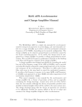
2.3.2.1.- Adaptación de la tensión de salida.
La variable que evalúa el control Entrada-Salida es la tensión de la salida del
convertidor, pero la señal que obtenemos a la salida es una tensión que varia entre los 18 V
y los 20.5 V, por lo que debemos realizar un circuito que adapte la tensión de salida a una
tensión que la pueda tratar el microcontrolador ya que este solo puede leer tensiones entre
0 y 5 V.
Para un mejor funcionamiento del circuito del convertidor y poder tener una mayor
resolución la conversión se realizará entre 0 y 2.5 V, pero el circuito generado podrá ser
utilizado para un margen mayor de tensiones para un futuro control, ya que puede dar
tensiones entre 0 y 5 V.
38
Memoria de cálculo
Control mediante Linealización Entrada-Salida
Tensión de salida ( V )
Obteniendo una señal entre 0 y 5V para luego hacer la conversión de una manera
óptima.
6
5
4
3
2
1
0
17
19
21
23
Tensión de entrada ( V )
Figura 2.7. Relación entrada-salida del sensor de tensión.
El circuito que se realiza para adaptar el señal está formado por dos etapas, la
primera etapa es un amplificador diferencial, que adapta la tensión de salida a una tensión
más reducida. La segunda etapa es un amplificador no inversor que ajusta el señal entre 0 y
5 V.
Vcc + 5 V
Vcc + 5 V
R41
140k
R42
5
R46
100k
10k
2
3
Vo
R44
10k
1
Vo sense
2
TLC2272IN
TLC2272IN
1
R45
5
82k
4
U14
+
R43
-
4
U15
3 +
R47
100k
10k
Vcc + 5 V
2
P49
2
20k
P48
1
20k
1
Figura 2.8. Sensor de tensión.
La expresión del primer operacional es:
Vo1 =
R 44·P 48
R 42
 R 42 
× Vcc
× 1 +
 × Vo −
R 43 + R 44 + P 48 
R 41 
R 41
(2.13)
La expresión del segundo operacional (Amplificador no inversor) es:
R 47 

Vo sense = 1 +
 × Vo1
R 45 + P 49 

(2.14)
39
Memoria de cálculo
Control mediante Linealización Entrada-Salida
Para un mejor funcionamiento de los amplificadores operacionales se ha optado
polarizarlos alrededor de la mitad de la tensión de alimentación (+5V), más o menos a 2.5
V, por lo tanto la tensión a la entrada no inversora del primer operacional tiene la siguiente
expresión:
V + ≈ 2.5V =
R 44·P 48
× Vo
R 43 + R 44 + P 48
(2.15)
Suponiendo que la tensión Vo será aproximadamente 19 V, el valor de R43, R44 y
el P48 serán de:
R44 = 10 kΩ.
R43 = 82 kΩ.
P48 = 20 kΩ.
Si el valor de la entrada Vo es menor que 19 V el valor de la salida del circuito total
tiene que ser 0 V (Vcc-) y si el valor de la entrada es 20.5 V el valor de la salida tiene que
ser 2.5 V.
Aplicando la ecuación (2.13) y teniendo en cuenta la primera condición:
La salida será igual a 0 V si Vin < 19 V.
0=
R 44 + P 48
R 42
 R 42 
·1 +
·5
·19 −
R 43 + R 44 + P 48 
R 41 
R 41
(2.16)
Suponiendo que el valor del potenciómetro es 0 Ω, ya que este se utiliza para un
mejor ajuste de la tensión de entrada, obtenemos la relación de R41 y R42.
0=
10000  R 42 
R 42
·1 +
·5
·19 −
92000 
R 41 
R 41
19  R 41 + R 42 
R 42
·
·5 =

9.2 
R 41
R 41 
(2.18)
R 42 19
=
R 41 27
R41 = 140 kΩ.
R42 = 100 kΩ.
40
Memoria de cálculo
Control mediante Linealización Entrada-Salida
Como podemos observar los valores de R41 y R42 no concuerdan con el valor de la
relación calculada, el potenciómetro P48 será el encargado de conseguir de forma indirecta
la relación deseada.
Si la entrada es de 20.5 V la salida del primer operacional tendrá el siguiente valor:
X =
19
10000  19 
×5
× 1 +  × 20.5 −
27
92000  27 
(2.19)
X = 0.277
La salida final de la etapa tiene que ser de 2.5 V, aplicando la ecuación (2.14) la
relación de R47/R45 tiene que ser:
 R 47 
2.5 = 1 +
 × 0.277
R 45 

9 = 1+
(2.20)
R 47
R 47
⇔
=8
R 45
R 45
R47 = 100 kΩ.
R45 = 10 kΩ.
El potenciómetro P49 es el encargado de conseguir la relación de R47/R45 deseada
y se ha escogido un valor de:
P49 = 20 kΩ.
La función de R46 es el de la polarización del segundo operacional y su valor es de:
R46 = 10 kΩ.
2.3.2.2.- Adaptación de las intensidades de las bobinas.
Para poder obtener la intensidad que pasa por las bobinas se tiene que introducir
una resistencia serie ya que la tensión en las bobinas no se puede medir en bornes de estas
ya que hay variaciones elevadas de tensión y no de intensidad, por eso se introduce una
resistencia serie, en la cual mediremos la tensión y de esta manera podremos saber la
intensidad que pasa por la bobina. Esta resistencia debe de ser pequeña ya que no
queremos perder rendimiento en el convertidor Boost.
41
Memoria de cálculo
Control mediante Linealización Entrada-Salida
Para la realización del sensado de corriente se utiliza un amplificador diferencial de
instrumentación ya que la tensión se debe referenciar a masa y se debe dar una ganancia
para poder tener la relación tensión corriente deseada.
La resistencia a utilizar será de 0.25 Ω, por lo que se tendrá que dar una ganancia
de 4 para que al realizar la conversión A/D tengamos el valor de la corriente.
El circuito utilizado es el siguiente:
3
I1 +
U1
5
R1
+
4
33k
2
R2
R11
R10
1
10k
10k
TLC2274IN
Vcc + 5 V
Vcc +5 V
10k
2
4
10k
3
20k
R4
1
R7
10k
I1 sense
5
U2
TLC2274IN
-
33k
R8
1
+
4
3
I1 -
TLC2274IN
1
Vcc + 5 V
2
R3
10k
U3
+
R6
P5
-
2
10k
5
R9
10k
Figura 2.9. Sensor de corriente 1.
La señal Vs + corresponde a la tensión más elevada de la resistencia serie de la
bobina 1 que en principio será una tensión constante de 12 V, la alimentación del
convertidor, y la señal Vs – será la menor tensión de la resistencia serie de la bobina 1.
El divisor de tensión a la entrada del amplificador de instrumentación sirve para
disminuir la tensión en modo común y para referenciar la tensión a masa, para que el
amplificador pueda trabajar en una zona de trabajo óptima.
La función del amplificador es la siguiente:
Vo =
R 4 R8  2·R6 
· ·1 +
·[Vs(+) − Vs(−)]
R 3 + R 4 R9 
P4 
(2.21)
Suponiendo que R7 = R6, R9 = R11, R10 = R8, R3 = R1, R4 = R2.
Los dos amplificadores diferenciales se diseñarán para tener una relación intensidad
tensión de:
Vo =
2.5
= 1A.
2.5
(2.22)
Al tener un voltio a la salida del amplificador de instrumentación querrá decir que
pasa un amperio por la resistencia serie de la bobina.
42
Memoria de cálculo
Control mediante Linealización Entrada-Salida
2,5
Voltage (V)
2
1,5
1
0,5
0
0
0,5
1
1,5
2
2,5
Intensidad (A)
Figura 2.10. Relación intensidad tensión.
Para poder obtener la relación intensidad tensión utilizaremos el potenciómetro para
obtener la ganancia deseada.
La ganancia total que deberá darnos el amplificador diferencial será:
Ganancia =
Tensión de salida
Tensión de entrada
(2.23)
La tensión de salida tiene que ser 2.5 V cuando la intensidad que pasa por la bobina
sea de 2.5 A, por tanto aplicando la fórmula de la ganancia:
G=
2.5V
=4
0.25Ω × 2.5 A
(2.24)
Para que el amplificador trabaje a la mitad de la tensión de alimentación, que será
2.5 V la relación de las resistencias que referencian a masa para el sensor de corriente de
la bobina 1 serán:
R1
I1 +
33k
R2
10k
R4
R3
10k
I1 -
33k
Figura 2.11. Referencia a masa sensor de corriente 1.
43
Memoria de cálculo
Control mediante Linealización Entrada-Salida
V+ =
R4
R4
R 4 2.5
·I1− =
·12V = 2.5V ⇒
=
R3 + R 4
R3 + R 4
R3 9.5
(2.25)
R4 = R2 = 10kΩ
R3 = R1 = 33kΩ
R10 = R8 = 10kΩ
R7 = R6 = 10kΩ
R9 = R11 = 10kΩ
3
I2 +
U5
5
R13
4
75k
+
R22
1
-
10k
TLC2274IN
2
R14
R23
10k
Vcc + 5 V
Vcc +5 V
10k
2
P17
R16
10k
3
20k
R19
1
10k
U7
TLC2274IN
1
I2 sense
+
2
4
10k
-
R18
5
Vcc + 5 V
U6
2
75k
TLC2274IN
R20
1
+
I2 -
3
-
4
R15
10k
R21
10k
5
Figura 2.12. Sensor de corriente 2.
Para el segundo sensor de corriente tendremos que la tensión que hay en bornes a la
resistencia a sensar será de unos 20 V, para que el amplificador se polarice a la mitad de la
tensión de alimentación, la relación del divisor de entrada será:
R13
I2 +
75k
R14
10k
R16
10k
R15
I2 -
75k
Figura 2.13. Referencia a masa sensor de corriente 2.
44
Memoria de cálculo
Control mediante Linealización Entrada-Salida
V+ =
R16
R16
R16 2.5
·I 2 − =
·20V = 2.5V ⇒
=
R15 + R16
R15 + R16
R15 17.5
(2.26)
R16 = R14 = 10kΩ
R15 = R13 = 75kΩ
R22 = R20 = 10kΩ
R18 = R19 = 10kΩ
R23 = R21 = 10kΩ
45
Memoria de cálculo
Control mediante Linealización Entrada-Salida
2.3.2.3.- Filtro Anti-Aliasing.
Este filtro se utilizará para eliminar las componentes de altas frecuencias para cada
señal a digitalizar.
Para la realización del filtro Anti-Aliasing se utilizará el filtro Butterworth, cuya
función de transferencia es:
H (s) =
wo2
s 2 + wo ⋅ s + wo2
(2.27)
Donde wo es la frecuencia de corte.
La frecuencia de muestreo del conversor A/D es de 8 kHz, por lo que la frecuencia
de corte del filtro Butterworth tiene que ser como mínimo la mitad de la frecuencia de
muestreo, es decir, menor que 4 kHz.
Para un mejor funcionamiento del filtro y mayor atenuación del ruido se escogerá
una frecuencia de corte del filtro de unos 2 kHz.
El filtro Butterworth es el que se presenta en la siguiente figura.
C11
10n
R37
Vcc + 5V
3
16k
U12
5
R38
16k
4
+
1
-
C12
2
TLC2274IN
2.2n
Figura 2.14. Filtro Butterworth.
Donde la función de transferencia es la siguiente:
1
R37·R38·C12·C11
H (s) =
1
1
1


+
+
s2 + s⋅

 R37·C11 R38·C11 R37·R38·C12·C11
(2.28)
Los valores de las resistencias R37 y R38 así como condensadores C11 y C12 se
han calculado para que se iguale la función de transferencia del filtro.
46
Memoria de cálculo
Control mediante Linealización Entrada-Salida
Según la ecuación del filtro Butterworth:
H (s) =
wo2
s 2 + wo ⋅ s + wo2
(2.27)
1
= wo2
R37·R38·C12·C11
wo =
1
R37·R38·C12·C11
=
1
1
+
R37·C11 R38·C12
Donde la variable wo = 2·π·f, y f es la frecuencia de corte del filtro de Butterworth.
wo = 2·π · f = 2·π ·2000 = 12566.4
rad
s
(2.29)
Los valores de las diferentes resistencias y condensadores para obtener un filtro
Butterworth de las características indicadas son:
R37 = 16000Ω.
R38 = 16000Ω.
C12 = 10nF.
C11 = 2,2nF.
Para obtener una señal correcta, con el mínimo de ruido en esta, viene dada esta
relación mediante la fórmula siguiente:
S
[dB] = 6.02 ⋅ b + 1.76
N
(2.30)
Donde b es el número de bits y S/N es la relación señal ruido.
Aplicando la formula (2.30), donde el número de bits de la conversión serán 8 para
el microcontrolador 80C537, obtenemos la relación señal ruido, que será:
S
[dB] = 6.02 ⋅ 8 + 1.76 = 49.92dB
N
(2.31)
47
Memoria de cálculo
Control mediante Linealización Entrada-Salida
Para realizar un filtro que para a la máxima componente frecuencial de 8 kHz tenga
una atenuación de 49.92 dB la frecuencia de corte del filtro sea de 2 kHz con las
resistencias y condensadores anteriormente calculadas, obtenemos:
H (2·π ·8000)
dB
=
(12566.4) 2
≈ 25db
(50265.6·i ) 2 + 12566.4 ⋅ 50265.6·i + (12566.4) 2
(2.32)
Para conseguir una atenuación de 49 dB a la frecuencia de 8 kHz se necesita otro
filtro Butterworth puesto en cascada, por lo que el conjunto del filtro-antialiasing será de
cuarto orden con una atenuación total de 50 dB.
C11
C13
10n
R33
5
R34
3 +
16k
16k
4
C12
10n
Vcc + 5V
U10
R35
R36
16k
16k
1
2
Vcc + 5V
TLC2274IN
5
3 +
4
U11
1
2
TLC2274IN
C14
2.2n
2.2n
Figura 2.15. Filtro anti-aliasing de cuarto orden.
48
Memoria de cálculo
Control mediante Linealización Entrada-Salida
2.3.2.4.- Generación del ciclo de trabajo.
En este apartado se explicará la adaptación de la señal cuadrada generada por el
microcontrolador, en el puerto 1 pin 2, para el encendido y apagado del transistor de
potencia.
Vin + 12 V
Vcc + 5 V
R50
10k
C15
C16
1u
1u
U19
U16A
1
P 1.2
1
2
3
2
3
4
7400
R51
10k
5
6
Vb
Vcc
IN
8
R52
ERROR
COM
OUT
7
Gate
12 1/2 W
Vs
Cs
C17
10n
R53
100k
D4
15 V
IR 2125
Figura 2.16. Circuito de disparo del transistor de potencia.
Una vez generada la señal cuadrada por el microcontrolador, en el puerto 1 pin 2,
esta variará según el tiempo que este a nivel alto o a nivel bajo, pero siempre con el mismo
periodo, la tensión variará entre 0 y 5 V.
Vcc + 5 V
R50
10k
U16A
1
P 1.2
3
2
7400
Figura 2.17. Circuito inversor.
En el microcontrolador 80C537 se da el problema que cada vez que se da el RESET
del microcontrolador ya sea por el pulsador o por el Watch Dog Timer todos los puertos
quedan a nivel alto por lo que si estuviera el transistor de potencia conectado, estaría
conectado hasta que no se volviera a programar el microcontrolador, pudiéndose dañar al
pasar una gran corriente, ya que se produce el cortocircuito de la fuente con la bobina.
Se ha optado por la introducción de un inversor, de esta manera al realizarse el
RESET del microcontrolador, a la salida del inversor quedaría a nivel bajo, no conduciendo
el transistor de potencia.
49
Memoria de cálculo
Control mediante Linealización Entrada-Salida
Una manera sencilla de realizar un inversor es la introducción de una puerta Nand,
cortocircuitando las entradas.
X1
X2
Out
0
0
1
0
1
1
1
0
1
1
1
0
Tabla 2.1. Función Nand.
La resistencia R50 Pull up, sirve por si se desconectara el microcontrolador no
quedara el transistor de potencia en conducción.
Vin + 12 V
C15
C16
1u
1u
U19
1
2
3
4
5
6
R51
10k
Vcc
IN
ERROR
COM
Vb
OUT
8
7
Vs
Cs
IR 2125
Figura 2.18. Driver IR2125.
El driver IR2125 se trata de un integrado que sirve para disparar transistores de
potencia ya que este tipo de transistores tienen una gran capacidad entre puerta y surtidor
lo que hace imposible dispararlos a través del puerto del microcontrolador. El
funcionamiento es sencillo ya que puede generar una señal cuadrada a una tensión más
elevada, en nuestro caso 12 V,con un tiempo de subida y bajada de unos 150 ns.
Este driver se ha configurado en Low Side ya que el surtidor del transistor de
potencia esta a masa, típica configuración en convertidores Boost, por lo que no hace falta
la tensión Bootstrap ( tensión de referencia ), típica en convertidores Buck
La resistencia R51 Pull down sirve por si se desconecta la etapa de control con la de
potencia, no pudiera quedar nunca en conducción el transistor de potencia.
El driver tiene que estar lo más cerca posible del transistor de potencia para evitar
el ruido. Por esto el driver se ha introducido en la placa de potencia.
50
Memoria de cálculo
Control mediante Linealización Entrada-Salida
R52
Gate
12 1/2 W
C17
10n
R53
100k
D4
15 V
Figura 2.19. Protección del transistor de potencia.
El condensador C17 sirve para eliminar las componentes frecuenciales altas, ya que
se pueden producir conmutaciones no deseadas cuando el driver pasa de 0 a 12 V y
viceversa.
La resistencia R53 Pull down sirve por si en un momento no se conecta el driver y
el transistor de potencia nunca pueda pasar al estado de conducción.
La resistencia R52 sirve para aumentar el tiempo de conmutación ya que entre la
puerta y el surtidor del transistor de potencia hay una capacidad de unos 2 nF por lo que el
circuito RC queda:
1
R52·C GS
41.6·10 6
H (s) =
=
⇒ τ = R52·C GS = 24ns
1
s + 41.6·10 6
s+
R52·C GS
(2.33)
Podemos observar que el tiempo de conmutación es más pequeño que el tiempo de
conmutación del driver que es del orden de 150 ns.
El diodo zener que hay entre la puerta y el surtidor sirve para eliminar las tensiones
negativas y las tensiones positivas de más de 15 V, que podrían dañar el transistor de
potencia.
51
Memoria de cálculo
Control mediante Linealización Entrada-Salida
2.3.2.5.- Alimentación de la placa de control.
Al tener que alimentar la placa de control mediante una tensión continua de 5 V se
ha optado por la introducción de una fuente lineal de tensión, mediante el integrado
LM7805. Este integrado suministra a la salida una tensión constante de 5 V que se puede
conectar a las diferentes alimentaciones de los amplificadores operacionales del circuito de
la placa de control.
Esta familia de integrados se pueden alimentar a tensiones elevadas, para que
puedan empezar a conducir deben de tener en su entrada una tensión 2 V superior a la
tensión que deben de tener a la salida, por lo que si se alimenta a la tensión de alimentación
de la placa de potencia el regulador funciona correctamente, por lo que no hace falta tener
dos fuentes de alimentación.
Este tipo de integrados tienen el problema que sus rendimientos son muy pequeños,
del orden del 50%, ya que en ellos se pierde la diferencia de tensión entre entrada y salida.
Se podría haber optado por la implementación de un pequeño Buck, reductor, con un
rendimiento mucho mas elevado, pero por la pequeña potencia que consume la etapa de
control, se descarto.
D1
Vin +12 V
1
2
1
3
1N4007
2
22u
+VS
GND
VOUT
2
7805
2
C1
1
U4
D2
100n
2191L
2
C2
1
Vcc + 5V
C3
1
100n
R12
1k
Figura 2.20. Fuente de alimentación.
El diodo de la entrada 1N4007 sirve por si se conecta erróneamente la tensión de
entrada de la placa de control, de esta manera las tensiones nunca pueden estar invertidas.
El condensador C1 es del tipo electrolítico, ya que este tipo de condensadores
tienen una relación tamaño capacidad elevada, sirve para almacenar energía en los
momentos que la placa pueda necesitarla en mayor o menor medida.
Los condensadores C2 y C3 sirven para eliminar de una manera rápida la subida de
tensión provocada por los armónicos de altas frecuencias, el condensador C2 elimina las
tensiones elevadas en la entrada y el condensador C3 las elimina en la salida.
Se ha optado por la introducción de un diodo LED para reconocer de una manera
sencilla y visual si la placa de control está alimentada correctamente.
52
Memoria de cálculo
Control mediante Linealización Entrada-Salida
2.3.2.6.- Conversión A/D.
El conversor analógico digital que se utiliza para realizar la conversión ya que se
encuentra integrado en el mismo microcontrolador. Se trata de un conversor de 8 bits, por
tanto la señal que se puede adquirir puede llegar a 256 ( 2 8 ) estados diferentes.
La entrada analógica posible no puede ser negativa y no puede exceder de los 5 V,
esto implica que tenemos una resolución máxima de:
Resolución máxima =
5V
= 19,53125 mV / estado
256 estados
(2.34)
En nuestro caso, la señal de entrada tiene un rango entre 0 y 2.5 V, y la resolución a
que se puede llegar es:
Resolución =
2.5 V
= 9,765625 mV / estado.
256 estados
(2.35)
Por tanto cualquier cambio de tensión en las señales a digitalizar de la planta
(convertidor conmutado) mayor que 9,765625 mV, el sistema de control lo detectará.
El tiempo que tarda en obtener el valor digital a partir del valor analógico de la
señal es en nuestro caso para el microcontrolador 80C537 a 12 MHz es de:
Tiempo de conversión = 13 µseg
Para otras especificaciones se puede mirar el manual técnico del microcontrolador,
anexo 3.
53
Memoria de cálculo
Control mediante Linealización Entrada-Salida
2.3.2.7.- Control por Linealización Entrada-Salida.
Este control está implementado de forma digital, en el microcontrolador 80C537 de
Siemens®.
La finalidad de este control es la de obtener un ciclo de trabajo mediante la tensión
de salidas y las intensidades que pasan por las bobinas del convertidor Boost con filtro de
salida. Una vez obtenidas las señales digitalizadas se calcula el ciclo de trabajo para el
nuevo periodo. Un primer diagrama de flujo mostrado en la figura 16 describe de forma
muy general el algoritmo implementado para realizar el control.
Conversión A/D
de las señales
Calculo del ciclo
de trabajo
Generación de la
señal cuadrada
Actualización
del ciclo de
trabajo
Figura 2.21. Diagrama de Flujo del control.
En el microcontrolador se debe de implementar el programa que realice el diagrama
de flujo anterior. La frecuencia en la cual el programa ha de obtener la salida de la señal
cuadrada actualizada es de 7 kHz. Por tanto el tiempo máximo de ejecución es de 142
µseg. Teniendo en cuenta que el reloj está oscilando a una frecuencia de 12 MHz y que
cada instrucción requiere como mínimo, instrucciones sencillas, 12 ciclos, el programa no
puede tener mas de 142 instrucciones sencillas.
Las instrucciones complejas como la multiplicación y la división en este
microcontrolador para variables enteras sin signo tardan:
División enteros sin signo
→
Multiplicación enteros sin signo
24 µseg.
→
16 µseg.
54
Memoria de cálculo
Control mediante Linealización Entrada-Salida
Para la realización del sistema de control necesitaremos unas variables del circuito
de potencia que irán variando a lo largo del tiempo, según la carga y la variación de la
fuente de alimentación.
El sistema de control mediante Linealización Entrada-Salida no es muy difícil de
implementar, mediante el microcontrolador 80C537, ya que este microcontrolador permite
la realización de divisiones y multiplicaciones mediante hardware, también gracias al
programa proview32 nos permite programarlo mediante código C, mucho mas fácil de
implementar que si fuera en código ensamblador. El programa proview32 genera un
fichero en hexadecimal que nos permite programar la EPROM o la RAM del
microcontrolador.
Una vez obtenido las señales de la tensión de salida, la intensidad que pasa por la
bobina 1 y la intensidad que pasa por la bobina 2, solo nos falta aplicar la fórmula del
control por Linealización por Entrada-Salida para obtener el ciclo de trabajo.
La siguiente fórmula da la ley de control por Linealización Entrada-Salida:
duty =
Donde:
-
IL1 − IL 2 + k ·(Vo _ deseada − Vo)
IL1
(2.36)
Duty es el ciclo de trabajo.
IL1 es la intensidad que pasa por la bobina 1.
IL2 es la intensidad que pasa por la bobina 2.
Vo_deseada es la tensión de salida que queremos conseguir.
Vo es la tensión real que hay en la salida del convertidor.
C1
k es
·(W − 1) , es la constante proporcional del control PI.
T
C1 es el condensador que hay después del diodo.
T es el periodo.
W es un valor entre 0 y 1.
A continuación se explicara el algoritmo de control que se ha grabado en la
EPROM de la placa Altair 537, que lleva incorporado el microcontrolador 80C537.
55
Memoria de cálculo
Control mediante Linealización Entrada-Salida
Programa Principal.
INICIO
Inicialización del
Watch Dog Timer.
Iniciado a 512 µseg.
Inicialización del Timer 0.
Contador de 8 bits.
Genera una señal cuadrada de 142 µseg
Duty cycle del 50 %.
Inicialización de las interrupciones.
Habilitar interrupción Timer 0.
Habilitar interrupción conversor A/D.
Prioridad del Timer 0 mayor que el
conversor A/D.
Inicialización del conversor A/D.
Seleccionar el puerto 7 pin 0 para la
primera conversión.
Inicio conversión entre 0 y 2.5 V.
PROGRAMA PRINCIPAL
Bucle infinito.
56
Memoria de cálculo
Control mediante Linealización Entrada-Salida
Interrupción del Timer 0.
Inicio Interrupción
Del Timer 0.
Puesta a cero del
Watch Dog Timer
¿Que valor tiene
la variable reloj?
reloj == 1
reloj == 0
Reloj = 0.
Reloj = 1.
Introducimos en la parte baja
del Timer 0 el tiempo de
conducción del transistor de
potencia t = Toff.
Introducimos en la parte
baja del Timer 0 el tiempo
de conducción del transistor
de potencia t = Ton.
Fin de Interrupción
57
Memoria de cálculo
Control mediante Linealización Entrada-Salida
Interrupción del conversor A/D.
Inicio Interrupción
del conversor A/D
Guardar el valor de la conversión
en la variable valor
¿Qué valor tiene la
variable ad_con?
ad _ con == 0
ad _ con == 1
Seleccionar el P7.1 ( I1b )
para la próxima
conversión.
Seleccionar el P7.2 ( I2b )
para
la
próxima
conversión.
Guardar la tensión de
salida ( Vob ).
Guardar la intensidad 1
( I1b ).
ad _ con == 2
BLOQUE
A
Nuevo valor para
ad_con = 1.
Nuevo valor para
ad_con = 2.
Comienza la próxima
conversión entre 0 y 2.5 V
Comienza la próxima
conversión entre 0 y 2.5 V
Fin de Interrupción
58
Memoria de cálculo
Control mediante Linealización Entrada-Salida
Interrupción del conversor A/D. BLOQUE A.
Seleccionar el P7.0 ( Vo )
para
la
próxima
conversión.
Guardar la intensidad 2
( I2b ).
Nuevo valor
ad_con = 0.
para
Cálculo del ciclo de trabajo.
I1b − I 2b +
duty =
(Vo _ des − Vob)
W
·T
I1b
Comienza
la
próxima
conversión entre 0 y 2.5 V.
¿Qué valor tiene
la variable Duty?
duty > 90 µs
duty < 90 µs
El ciclo será fijo, será
del 50 %. Asignándose
un valor a las variables
Ton y Toff.
Calculo de las variables
del ciclo de trabajo para
el próximo periodo.
Ton y Toff.
59
Memoria de cálculo
Control mediante Linealización Entrada-Salida
2.4.- Parámetros principales de la planta.
El convertidor conmutado DC/DC Boost elevador sobre el que se ha explicado el
control tiene como parámetros principales los siguientes valores:
PARÁMETRO
SIMBOLO
Tensión de entrada.
Vin
Tensión de salida
Vo
Inductancia en la bobina 1
L1
Inductancia en la bobina 2
L2
Capacidad de salida
C1
Capacidad del filtro
C2
Carga de salida
R28-R27
Resistencia de sensado 1
R24
Resistencia de sensado 2
R25
Resistencia en la bobina 1
RS1
Resistencia en la bobina 2
RS2
Resistencia al MOSFET
RDS
Caída de tensión en el diodo
Vd (on)
VALOR
12 V
18-20 V
0.69 mH
1.22 mH
46.2 µF
124.2 µF
48-28 Ω
0.25 Ω
0.25 Ω
0.4 Ω
0.9 Ω
0.07 Ω
0.25 V
Tabla 2.2. Parámetros fijos de la planta.
CÁLCULOS
Corriente en la bobina 1 media carga.
Corriente en la bobina 1 toda la carga.
Corriente en la bobina 2 media carga.
Corriente en la bobina 2 toda la carga.
Potencia de entrada media carga.
Potencia de salida media carga.
Potencia de entrada toda la carga.
Potencia de salida toda la carga.
Rendimiento a media carga.
Rendimiento con toda la carga.
SÍMBOLO
IL1
IL1
IL2
IL2
Pi
Po
Pi
Po
η
η
VALOR
0.8 A
1.08
0.425 A
0.65 A
9.6 W
8.67 W
13.68 W
11.9 W
90.3 %
87 %
Tabla 2.3. Parámetros variables de la planta.
60
Memoria de cálculo
Control mediante Linealización Entrada-Salida
2.5.- Listado de todos los componentes calculados.
COMPONENTE
R1
R2
R3
R4
P5
R6
R7
R8
R9
R10
R11
R12
R13
R14
R15
R16
P17
R18
R19
R20
R21
R22
R23
R24
R25
R26
R27
R28
R29
R30
R31
R32
R33
R34
R35
R36
R37
R38
R39
R40
R41
VALOR
33 kΩ
10 kΩ
33 kΩ
10 kΩ
20 kΩ
10 kΩ
10 kΩ
10 kΩ
10 kΩ
10 kΩ
10 kΩ
1 kΩ
75 kΩ
10 kΩ
75 kΩ
10 kΩ
20 kΩ
10 kΩ
10 kΩ
10 kΩ
10 kΩ
10 kΩ
10 kΩ
0.25 Ω
0.25 Ω
10 Ω
48 Ω
68 Ω
16 kΩ
16 kΩ
16 kΩ
16 kΩ
16 kΩ
16 kΩ
16 kΩ
16 kΩ
16 kΩ
16 kΩ
16 kΩ
16 kΩ
140 kΩ
61
Memoria de cálculo
Control mediante Linealización Entrada-Salida
R42
R43
R44
R45
R46
R47
P48
P49
R50
R51
R52
R53
C1
C2
C3
C4
C5
C6
C7
C8
C9
C10
C11
C12
C13
C14
C15
C16
C17
C18
C19
C20
C21
C22
C23
C24
C25
100 kΩ
82 kΩ
10 kΩ
10 kΩ
10 kΩ
100 kΩ
20 kΩ
20 kΩ
10 kΩ
10 kΩ
12 Ω
100 kΩ
22 µF
100 nF
100 nF
1 nF
22 µF
22 µF
2.2 µF
22 µF
100 µF
2.2 µF
10 nF
2.2 nF
10 nF
2.2 nF
10 nF
2.2 nF
10 nF
2.2 nF
10 nF
2.2 nF
10 nF
2.2 nF
1 µF
1 µF
10 nF
Tabla 2.4. Componentes calculados.
62
Memoria de cálculo
3.- PLANOS.
5
4
3
2
1
D
D
I1 +
I1 -
L1
R24
1
C
I2 +
I2 -
R25
D3
2
1
Vo
2
1
L2
2
C
Vin + 12 V
0.25 6W
0.69m
BYW 29
2
0.25 6W
1.22 m
R26
10 1/2 W
1
1
Q1
3
Gate
2
2
2
2
2
2
2
2
2
BUK 455
C5
2
C4
1
1 22u
C6
1 22u
C7
C8
1 2.2u
1 22u
C9
1 100u
C10
1 2.2u
R28
R27
47 12 W
68 12 W
1
1
1n
B
B
A
A
Title
ETAPA DE POTENCIA
Size
A4
Date:
5
4
3
Document Number
Rev
001
0
AGOSTO 2003
2
Sheet
1
of
1
7
5
4
3
2
1
D
D
5
R1
U1
3 +
I1 +
33k
4
-
R11
10k
2
R2
C
R10
1
10k
10k
TLC2274IN
Vcc + 5 V
Vcc +5 V
2
4
3
20k
R4
1
R7 10k
TLC2274IN
1
I1 sense
+
10k
-
R6
P5
C
U3
2
5
10k
Vcc + 5 V
2
3
I1 33k
TLC2274IN
R8
1
+
B
4
-
R3
U2
10k
B
R9
5
10k
A
A
Title
SENSOR DE CORRIENTE 1
Size
A4
Date:
5
4
3
Document Number
Rev
002
0
AGOSTO 2003
2
Sheet
2
of
1
7
5
4
3
2
1
D
D
U5
5
R13
3 +
I2 +
75k
4
2
R14
R22
R23
10k
10k
1
10k
TLC2274IN
Vcc + 5 V
Vcc +5 V
U7
2
10k
4
P17
R16
3
20k
R19
1
10k
TLC2274IN
C
1
I2 sense
+
R18
2
-
C
5
10k
Vcc + 5 V
2
75k
R20
1
+
3
I2 -
TLC2274IN
-
4
R15
U6
10k
R21
10k
5
B
B
A
A
Title
SENSOR DE CORRIENTE 2
Size
A4
Date:
5
4
3
Document Number
Rev
003
0
AGOSTO 2003
2
Sheet
3
of
1
7
5
4
3
2
1
D
D
Vcc + 5 V
Vcc + 5 V
R41
140k
R42
5
R46
100k
U15
3 +
10k
4
C
2
1
Vo sense
-
U14
C
2
TLC2272IN
TLC2272IN
1
+
3
Vo
-
4
R43
R45
5
82k
R47
100k
10k
R44
10k
Vcc + 5 V
2
P49
2
20k
P48
B
1
B
20k
1
A
A
Title
SENSOR DE TENSIÓN
Size
A4
Date:
5
4
3
Document Number
Rev
004
0
AGOSTO 2003
2
Sheet
4
of
1
7
5
4
3
2
C11
1
C13
10n
10n
Vcc + 5V
Vcc + 5V
R29
D
5
R30
U8
R31
3 +
Vo sense
16k
16k
4
1
-
U9
3 +
16k
2
C12
5
R32
16k
4
TLC2274IN
1
PUERTO 7.0
2
2.2n
D
TLC2274IN
C14
2.2n
C15
C17
10n
Vcc + 5V
10n
C
C
Vcc + 5V
R33
U10
5
R34
3 +
I1 sense
16k
16k
4
R36
16k
16k
5
1
2
C16
R35
U11
3 +
4
TLC2274IN
1
PUERTO 7.1
2
2.2n
TLC2274IN
C18
2.2n
C19
C21
B
B
10n
10n
Vcc + 5V
Vcc + 5V
R37
5
R38
R39
3 +
I2 sense
16k
16k
4
5
R40
1
-
3 +
16k
2
C20
U12
16k
4
TLC2274IN
1
PUERTO 7.2
2
2.2n
U13
TLC2274IN
C22
2.2n
A
A
Title
FILTRO ANTI-ALIASING
Size
A4
Date:
5
4
3
Document Number
Rev
005
0
AGOSTO 2003
2
Sheet
5
of
1
7
5
4
3
2
1
D
D
Vin + 12 V
Vcc + 5 V
C23
R50
10k
C24
1u
1u
C
C
U19
U16A
1
1
2
3
P 1.2
2
3
4
7400
5
6
R51
10k
Vcc
IN
Vb
8
R52
ERROR
COM
OUT
7
Gate
12 1/2 W
Vs
Cs
R53
C25
100k
10n
D4
15 V
IR 2125
B
B
A
A
Title
DRIVER IR2125
Size
A4
Date:
5
4
3
Document Number
Rev
006
0
AGOSTO 2003
2
Sheet
6
of
1
7
5
4
3
2
1
D
D
C
C
D1
U4
1
2
1
3
Vin +12 V
1N4007
+VS
GND
VOUT
2
Vcc + 5V
D2
7805
2
2
C1
1
22u
C2
1
2191L
2
C3
100n
1
100n
R12
1k
B
B
A
A
Title
FUENTE DE ALIMENTACIÓN
Size
A4
Date:
5
4
3
Document Number
Rev
007
0
AGOSTO 2003
2
Sheet
7
of
1
7
Control mediante Linealización Entrada-salida.
Lamina 8
Lámina 8. Caja etapa de control.
Control mediante Linealización Entrada-salida.
Lamina 9
Lámina 9. Caja etapa de potencia.
4.- PRESUPUESTO.
Control mediante Linealización Entrada-Salida
4.- Presupuesto.
4.1.- Precios elementales.
4.1.1.- Capitulo 1: Diseño, Simulación e Implementación.
NÚMERO
A1000
A1001
A1002
A1003
UNIDADES
h
h
h
h
DESCRIPCIÓN
Estudio teórico y simulación.
Diseño del Hardware.
Diseño del software.
Montaje y puesta en marcha del equipo.
PRECIO
28
28
28
13,5
71
Presupuesto
Control mediante Linealización Entrada-Salida
4.1.2.- Capítulo 2: Material.
NÚMERO
B1000
B1001
B1002
B1003
B1004
B1005
B1006
B1007
B1008
B1009
B1010
B1011
B1012
B2000
B2001
B2002
B2003
B2100
B2200
B2300
B2303
B3000
B3001
B4000
B4001
B4100
B4200
UNIDADES
DESCRIPCIÓN
u
Resistencia de carbón 10 Ω, ±1%
tolerancia, ½ W.
u
Resistencia de carbón 12 Ω, ±1%
tolerancia, ½ W.
u
Resistencia de carbón 1 kΩ, ±1%
tolerancia, ¼ W.
u
Resistencia de carbón 10 kΩ, ±1%
tolerancia, ¼ W.
u
Resistencia de carbón 16 kΩ, ±1%
tolerancia, ¼ W.
u
Resistencia de carbón 33 kΩ, ±1%
tolerancia, ¼ W.
u
Resistencia de carbón 75 kΩ, ±1%
tolerancia, ¼ W.
u
Resistencia de carbón 82 kΩ, ±1%
tolerancia, ¼ W.
u
Resistencia de carbón 100 kΩ, ±1%
tolerancia, ¼ W.
u
Resistencia de carbón 140 kΩ, ±1%
tolerancia, ¼ W.
u
Resistencia cerámica 0.25 Ω, ±1%
tolerancia, 6 W.
u
Resistencia cerámica 47 Ω, ±5%
tolerancia, 12 W.
u
Resistencia cerámica 68 Ω, ±5%
tolerancia, 12 W.
u
Condensador de poliéster de 1 nF.
u
Condensador de poliéster de 2.2 nF.
u
Condensador de poliéster de 10 nF.
u
Condensador de poliéster de 100 nF.
u
Condensador de poliéster de 1 µF.
u
Condensador cerámico 2.2 µF.
u
Condensador electrolítico 22 µF, 50 V.
u
Condensador de papel de 100 µF, 50 V.
u
Zócalo torneado DIP100T 8 pins.
u
Zócalo torneado DIP100T 14 pins.
u
Circuito integrado TLC2272IN.
(2 Amplificadores Operacionales).
u
Circuito integrado TLC2274IN.
(4 Amplificadores Operacionales).
u
Circuito integrado DM74LS00.
(4 Puertas Nand).
u
Circuito integrado 7805.
(Fuente lineal).
de
PRECIO
0,04
de
0,04
de
0,04
de
0,04
de
0,04
de
0,04
de
0,04
de
0,04
de
0,04
de
0,04
de
0,55
de
0,45
de
0,45
0,12
0,13
0,14
0,18
0,24
0,5
0,08
0,12
1,36
1,53
1,51
1,86
0,35
0,51
72
Presupuesto
Control mediante Linealización Entrada-Salida
B5000
u
B6000
B6500
u
m
B7000
B7100
B7201
B7300
B7500
B7500
B8000
B8001
B9000
B9100
B9200
B9300
B9301
B9350
B9500
u
u
u
u
u
u
u
u
u
u
u
u
u
m
u
Potenciómetro multivuelta, ajuste horizontal
20 kΩ, ±10% de tolerancia, ¼ W.
Toroidal NTH039 Ariston.
Cable de cobre diámetro 0.6 mm
PIRESOLD
Diodo Zener 15 V.
Diodo Schottky BYW2950.
Diodo bipolar 1N4007.
Diodo led.
MOSFET de potencia BUK455.
Driver IR2125.
Tornillos.
Tuercas.
Interruptor 3 posiciones, montaje en caja.
Caja estanca 190x95x60 mm, PVC.
Conector hembra banana diámetro 4 mm.
Conector hembra cable plano 10 pines.
Conector macho cable plano 10 pines.
Cable plano 10 pines.
Placa de topos 150x80 mm
0,74
0,9
0,01
0,05
0,69
0,03
0,05
1,57
3,58
0,02
0,02
1,5
8,5
2,25
0,8
1,2
0,94
6,5
73
Presupuesto
Control mediante Linealización Entrada-Salida
4.2.- Anidamientos.
4.2.1.- Capítulo 1: Diseño, Simulación e Implementación.
NÚMERO
A1000
A1001
A1002
A1003
UNIDADES
h
h
h
h
DESCRIPCIÓN
Estudio teórico y simulación.
Diseño del Hardware.
Diseño del software.
Montaje y puesta en marcha del equipo.
CANTIDAD
25
15
8
52
74
Presupuesto
Control mediante Linealización Entrada-Salida
4.2.2.- Capítulo 2: Material.
NÚMERO
B1000
B1001
B1002
B1003
B1004
B1005
B1006
B1007
B1008
B1009
B1010
B1011
B1012
B2000
B2001
B2002
B2003
B2100
B2200
B2300
B2303
B3000
B3001
B4000
B4001
B4100
B4200
UNIDADES
DESCRIPCIÓN
u
Resistencia de carbón 10 Ω, ±1%
tolerancia, ½ W.
u
Resistencia de carbón 12 Ω, ±1%
tolerancia, ½ W.
u
Resistencia de carbón 1 kΩ, ±1%
tolerancia, ¼ W.
u
Resistencia de carbón 10 kΩ, ±1%
tolerancia, ¼ W.
u
Resistencia de carbón 16 kΩ, ±1%
tolerancia, ¼ W.
u
Resistencia de carbón 33 kΩ, ±1%
tolerancia, ¼ W.
u
Resistencia de carbón 75 kΩ, ±1%
tolerancia, ¼ W.
u
Resistencia de carbón 82 kΩ, ±1%
tolerancia, ¼ W.
u
Resistencia de carbón 100 kΩ, ±1%
tolerancia, ¼ W.
u
Resistencia de carbón 140 kΩ, ±1%
tolerancia, ¼ W.
u
Resistencia cerámica 0.25 Ω, ±1%
tolerancia, 6 W.
u
Resistencia cerámica 47 Ω, ±5%
tolerancia, 12 W.
u
Resistencia cerámica 68 Ω, ±5%
tolerancia, 12 W.
u
Condensador de poliéster de 1 nF.
u
Condensador de poliéster de 2.2 nF.
u
Condensador de poliéster de 10 nF.
u
Condensador de poliéster de 100 nF.
u
Condensador de poliéster de 1 µF.
u
Condensador cerámico 2.2 µF.
u
Condensador electrolítico 22 µF, 50 V.
u
Condensador de papel de 100 µF, 50 V.
u
Zócalo torneado DIP100T 8 pins.
u
Zócalo torneado DIP100T 14 pins.
u
Circuito integrado TLC2272IN.
(2 Amplificadores Operacionales).
u
Circuito integrado TLC2274IN.
(4 Amplificadores Operacionales).
u
Circuito integrado DM74LS00.
(4 Puertas Nand).
u
Circuito integrado 7805.
CANTIDAD
1
de
de
1
de
1
de
21
de
12
de
2
de
2
de
1
de
3
de
1
de
2
de
1
de
1
1
6
8
2
2
2
3
1
2
4
1
3
1
1
75
Presupuesto
Control mediante Linealización Entrada-Salida
B5000
u
B6000
B6500
u
m
B7000
B7100
B7201
B7300
B7500
B7500
B8000
B8001
B9000
B9100
B9200
B9300
B9301
B9350
B9500
u
u
u
u
u
u
u
u
u
u
u
u
u
m
u
(Fuente lineal).
Potenciómetro
multivuelta,
ajuste
horizontal 20 kΩ, ±10% de tolerancia, ¼
W.
Toroidal NTH039 Ariston.
Cable de cobre diámetro 0.6 mm
PIRESOLD
Diodo Zener 15 V.
Diodo Schottky BYW2950.
Diodo bipolar 1N4007.
Diodo led.
MOSFET de potencia BUK455.
Driver IR2125.
Tornillos.
Tuercas.
Interruptor 3 posiciones, montaje en caja.
Caja estanca 190x95x60 mm, PVC.
Conector hembra banana diámetro 4 mm.
Conector hembra cable plano 10 pines.
Conector macho cable plano 10 pines.
Cable plano 10 pines.
Placa de topos 150x80 mm
4
2
38,6
1
1
1
1
1
1
8
8
1
2
18
2
4
0,5
2
76
Presupuesto
Control mediante Linealización Entrada-Salida
4.3.- Aplicación de precios.
4.3.1.- Capitulo 1: Diseño, Simulación e Implementación.
NÚMERO
UNI.
DESCRIPCIÓN
PRECIO
CANT.
IMPORTE
A1000
h
Estudio teórico y simulación.
28
25
700
A1001
h
Diseño del Hardware.
28
15
420
A1002
h
Diseño del software.
28
8
224
A1003
h
Montaje y puesta en marcha
del equipo.
13,5
52
702
TOTAL CAPÍTULO 1: Diseño, Simulación e Implementación.
2046 €
77
Presupuesto
Control mediante Linealización Entrada-Salida
4.1.2.- Capítulo 2: Material.
NÚMERO
B1000
UNI.
u
B1001
u
B1002
u
B1003
u
B1004
u
B1005
u
B1006
u
B1007
u
B1008
u
B1009
u
B1010
u
B1011
u
B1012
u
B2000
B2001
B2002
B2003
B2100
B2200
B2300
B2303
B3000
B3001
B4000
u
u
u
u
u
u
u
u
u
u
u
B4001
u
B4100
u
B4200
u
B5000
u
B6000
B6500
u
m
B7000
u
DESCRIPCIÓN
Resistencia de carbón 10 Ω, ±1% de
tolerancia, ½ W.
Resistencia de carbón 12 Ω, ±1% de
tolerancia, ½ W.
Resistencia de carbón 1 kΩ, ±1% de
tolerancia, ¼ W.
Resistencia de carbón 10 kΩ, ±1% de
tolerancia, ¼ W.
Resistencia de carbón 16 kΩ, ±1% de
tolerancia, ¼ W.
Resistencia de carbón 33 kΩ, ±1% de
tolerancia, ¼ W.
Resistencia de carbón 75 kΩ, ±1% de
tolerancia, ¼ W.
Resistencia de carbón 82 kΩ, ±1% de
tolerancia, ¼ W.
Resistencia de carbón 100 kΩ, ±1% de
tolerancia, ¼ W.
Resistencia de carbón 140 kΩ, ±1% de
tolerancia, ¼ W.
Resistencia cerámica 0.25 Ω, ±1% de
tolerancia, 6 W.
Resistencia cerámica 47 Ω, ±5% de
tolerancia, 12 W.
Resistencia cerámica 68 Ω, ±5% de
tolerancia, 12 W.
Condensador de poliéster de 1 nF.
Condensador de poliéster de 2.2 nF.
Condensador de poliéster de 10 nF.
Condensador de poliéster de 100 nF.
Condensador de poliéster de 1 µF.
Condensador cerámico 2.2 µF.
Condensador electrolítico 22 µF, 50 V.
Condensador de papel de 100 µF, 50 V.
Zócalo torneado DIP100T 8 pins.
Zócalo torneado DIP100T 14 pins.
Circuito integrado TLC2272IN.
(2 Amplificadores Operacionales).
Circuito integrado TLC2274IN.
(4 Amplificadores Operacionales).
Circuito integrado DM74LS00.
(4 Puertas Nand).
Circuito integrado 7805.
(Fuente lineal).
Potenciómetro
multivuelta,
ajuste
horizontal 20 kΩ, ±10% de tol., ¼ W.
Toroidal NTH039 Ariston.
Cable de cobre diámetro 0.6 mm
PIRESOLD
Diodo Zener 15 V.
PRECIO
0,04
CANT.
1
IMPORTE
0,04
0,04
1
0,04
0,04
1
0,04
0,04
21
0,84
0,04
12
0,48
0,04
2
0,08
0,04
2
0,08
0,04
1
0,04
0,04
3
0,12
0,04
1
0,04
0,55
2
1,1
0,45
1
0,45
0,45
1
0,45
0,12
0,13
0,14
0,18
0,24
0,5
0,08
0,12
1,36
1,53
1,51
1
6
8
2
2
2
3
1
2
4
1
0,12
0,78
1,12
0,36
0,48
1
0,24
0,12
2,72
6,12
1,51
1,86
3
5,58
0,35
1
0,35
0,51
1
0,51
0,74
4
2,96
0,9
0,01
2
38,6
1,8
0,37
0,05
1
0,05
78
Presupuesto
Control mediante Linealización Entrada-Salida
B7100
B7201
B7300
B7500
B7500
B8000
B8001
B9000
u
u
u
u
u
u
u
u
B9100
B9200
u
u
B9300
B9301
B9350
B9500
u
u
m
u
Diodo Schottky BYW2950.
Diodo bipolar 1N4007.
Diodo led.
MOSFET de potencia BUK455.
Driver IR2125.
Tornillos.
Tuercas.
Interruptor 3 posiciones, montaje en
caja.
Caja estanca 190x95x60 mm, PVC.
Conector hembra banana diámetro 4
mm.
Conector hembra cable plano 10 pines.
Conector macho cable plano 10 pines.
Cable plano 10 pines.
Placa de topos 150x80 mm
TOTAL CAPÍTULO 2: Material.
0,69
0,03
0,05
1,57
3,58
0,02
0,02
1,5
1
1
1
1
1
8
8
1
0,69
0,03
0,05
1,57
3,58
0,16
0,16
1,5
8,5
2,25
2
18
17
40,5
0,8
1,2
0,94
6,5
2
4
0,5
2
1,6
1,2
0,47
13
110,3 €
79
Presupuesto
Control mediante Linealización Entrada-Salida
4.4.- Precio de ejecución por material.
Total capítulo 1................................................................................................2.046 €.
Total capítulo 2................................................................................................110,3 €.
Total presupuesto de ejecución por material................................................2.156,3 €.
4.5.- Precio de ejecución por contrato.
Total presupuesto de ejecución por material (*)..........................................2.156,3 €.
Gastos generales 13,00 % (*)........................................................................280,32 €.
Beneficio industrial 6,00 % (*).....................................................................129,38 €.
Precio total.......................................................................................................2566 €.
4.6.- Precio por licitación.
Precio total (**)................................................................................................2566 €.
I.V.A. 16,00 % (**).......................................................................................410,56 €.
Precio total por licitación.............................................................................2976,56 €.
4.7.- Resumen del presupuesto.
El presupuesto asciende a: 2976,56 euros.
(495.258 pesetas)
DOS MIL NOVECIENTOS SETENTA Y SEIS EUROS CON CINCUENTA Y
SEIS CÉNTIMOS.
(CUATROCIENTAS NOVENTA Y CINCO MIL DOSCIENTAS CINCUENTA
Y OCHO PESETAS).
Tarragona 5 de septiembre del 2003.
EL INGENIERO TÉCNICO ELECTRÓNICO.
LORENZO PUJOL MAYOL.
80
Presupuesto
5.- PLIEGO DE CONDICIONES.
Control mediante Linealización Entrada-Salida
5.- Pliego de condiciones.
5.1.- Disposiciones y abarque del pliego de condiciones.
5.1.1.- Objetivo del pliego.
El objetivo de este proyecto es el estudio de un convertidor Boost con filtro de
salida con un control por linealización entrada-salida. Este proyecto es un proyecto de
investigación, esto implica que el prototipo se ha diseñado teniendo en cuenta la
accesibilidad y la fiabilidad de estudio omitiendo su desarrollo industrial. En caso de una
futura aplicabilidad industrial se debería tener presente el pliego de condiciones, que tiene
como principal función regular las condiciones entre las partes contratantes considerando
los aspectos técnicos, facultativos, económicos y legales.
El pliego de condiciones define entre los otros los siguientes aspectos:
-
Obras que componen el proyecto.
Características exigibles a los materiales y componentes.
Detalles de la ejecución.
Programa de obras.
Dado el amplio abanico de detalles tratados si se presentan dudas a la hora de poner
en marcha el proyecto lo más recomendable es ponerse en contacto con el proyectista.
81
Pliego de condiciones
Control mediante Linealización Entrada-Salida
5.1.2.- Descripción general del montaje.
Las diferentes partes que componen la obra a realizar por parte del instalador,
poniendo especial énfasis en el orden establecido, no efectuando una actividad concreta sin
haber realizado previamente la anterior:
-
Encargo y compra de los componentes necesarios.
Construcción de los inductores.
Fabricación de la placa de circuito impreso.
Montaje de los componentes en la placa.
Montaje de la caja.
Ajuste y comprobación de los parámetros para el buen funcionamiento.
Interconexión de los diferentes módulos.
Puesta en marcha del equipo.
Controles de calidad y fiabilidad.
Mantenimiento para el correcto funcionamiento del sistema.
Todas las partes que en conjunto forman la obra de este proyecto, tendrán que ser
ejecutadas por montadores calificados, sometiéndose a las normas de la Comunidad
Autónoma Europea, países o incluso comunidades internacionales que se tengan previstas
para este tipo de montajes, no haciéndose responsable el proyectista de los desperfectos
ocasionados por su incumplimiento.
82
Pliego de condiciones
Control mediante Linealización Entrada-Salida
5.2.- Condiciones de los materiales.
En este apartado se explican las características técnicas exigibles de los
componentes presentes en la ejecución de la obra.
5.2.1.- Especificaciones eléctricas.
5.2.1.1.- Placas de circuito impreso.
Todos los circuitos se realizarán sobre placas de fibra de vidrio de sensibilidad
positiva, en diferentes medidas, utilizándose una sola cara o de doble cara según el diseño.
5.2.1.2.- Conductores eléctricos.
Los conductores utilizados serán internos a excepción de la alimentación y de la
interconexión entre placas que reunirán condiciones especiales requeridas para los
conductores expuestos al exterior. Cabe comentar que la obra tendrá lugar dentro de un
laboratorio o una industria. Los cables de interconexión entre placas y de la fuente de
alimentación están constituidos por un cable unipolar debidamente aislado con una sección
de 1.5 mm2.
5.2.1.3.- Componentes pasivos.
Los componentes pasivos utilizados en el proyecto son los disponibles
tecnológicamente en el momento de la realización del proyecto. Las características técnicas
se han introducido en el Anexo.
5.2.1.4.- Componentes activos.
Los componentes pasivos utilizados en el proyecto son los disponibles
tecnológicamente en el momento de la realización del proyecto. Las características técnicas
se han introducido en el Anexo.
83
Pliego de condiciones
Control mediante Linealización Entrada-Salida
5.2.1.5.- Zócalos torneados tipo D.I.L.
Todos los circuitos integrados que aparecen dispondrán de un zócalo para su unión
con la placa de circuito impreso. Estos zócalos son del tipo D.I.L (“Dual IN Line”) de
contacto mecanizado de gran cantidad y de perfil bajo, formados por contactos internos de
tipo cuatro dedos (3-5 µm) de estaño sobre una base de cobre-berilio niquelado y con un
recubrimiento de carbón estañado. También están amoldados mediante un poliéster negro
con fibra de vidrio ignífuga, sus características se encuentran en la tabla 6.1.
Margen de temperaturas
Resistencia de contacto
Resistencia de aislamiento
Fuerza de inserción por contacto
Fuerza de extracción por contacto
Fuerza de retención por contacto
-55ºC a 125ºC
10mΩ (máximo)
1010 Ω
120 gr
80 gr
400 gr (mínimo)
Tabla 6.1. Características técnicas de los zócalos tipo D.I.L.
5.2.1.6.- Reglamento Electrotécnico de Baja Tensión.
Todos los aspectos técnicos de la instalación que, directa o indirectamente, estén
incluidos en el Reglamento Electrotécnico de Baja Tensión, tendrán que cumplir lo que se
disponga en las respectivas normas.
Las instrucciones más importantes relacionadas con la realización del proyecto son
las siguientes:
-
M.I.B.T.017
Instalaciones interiores o receptoras.
Prescripciones de carácter general.
-
M.I.B.T.029
Instalaciones a pequeñas tensiones.
-
M.I.B.T.030
Instalaciones a tensiones especiales.
-
M.I.B.T.031
Receptores. Prescripciones generales
-
M.I.B.T.035
Receptores. Transformadores y autotransformadores.
Reactancias y rectificadores. Condensadores.
-
M.I.B.T.044
Normas U.N.E. de obligado cumplimiento.
5.2.1.7.- Resistencias.
Es necesario establecer los extremos máximos y mínimos entre los que estarán
comprendidos las resistencias. La tolerancia marca estos valores que se expresan
normalmente como porcentajes del valor en ohmios asignados teóricamente. Se tendrá que
expresar su tolerancia y sumarla al valor nominal.
84
Pliego de condiciones
Control mediante Linealización Entrada-Salida
Existen resistencias con una gran precisión en el valor, el que implicar fijar
tolerancias muy bajas, pero se tendrá en cuenta que su precio aumenta considerablemente y
solamente serán necesarias en aplicaciones muy específicas estando normalmente
destinadas a usos generales las tolerancias estandarizadas de 5%, 10% y 20%.
Ateniéndose al valor ohmico y a la tolerancia, se establecen de forma estándar una
serie de valores, de forma que con ellos se pueda tener toda una gama de resistencias desde
1 ohmio en adelante, estos valores son los siguientes:
E6.- 1,1.5, 2.2, 3.3, 4.7, 6.8.
E12.- 1, 1.5, 1.8, 2.2, 2.7, 3.3, 3.9, 4.7, 5.6, 6.8, 8.2.
E24.- 1, 1.2, 1.3, 1.5, 1.6, 1.8, 2, 2.2, 2.4, 2.7, 3, 3.3, 3.6, 3.9, 4.3, 4.7, 5.1, 5.6, 5.2,
6.8, 7.5, 8.2, 9.8.
La serie E6 equivale a valores correspondientes a la tolerancia del 20%, la serie
E12 a valores definidos por el 10%, y la serie E24 a la de 5%.
El conjunto total de valores de toda la gama se obtiene multiplicando por 0.1, 1, 10,
100, 103, 104, 105, 106 o 107 la tabla anterior. Para evitar la utilización d eun número
elevado de ceros en la designación del valor de una resistencia, se utilizan las letras: k y M,
que designan un factor multiplicador de 103 y 106 respectivamente.
Para identificar el valor de una resistencia se utiliza un sistema por medio de
colores que permite cubrir toda la tabla anterior. A este sistema se le denomina código de
colores y consiste en pintar alrededor de la resistencia, en un extremo, cuatro anillos de
unos colores determinados, corresponden los dos primeros colores son los identificadores
del valor de la tabla de valores anteriores, el tercer color al numero de ceros que es
necesario añadir y el cuarto a la tolerancia.
La disipación de potencia en forma de calor que es capaz de soportar se ha de tener
en cuenta ya que la corriente que atraviesa la resistencia por una cierta energía que se
utiliza para vencer la dificultad que presenta su paso, esta energía se transforma en calor, y
la cantidad de este es inversamente proporcional al valor óhmico de la resistencia. Por
tanto para un valor fijo de resistencia, se disipará en el ambiente una cantidad de calor
cuatro veces mayor si circula una corriente de 2 A, que si lo hace una de 1 A. La máxima
disipación de potencia que puede soportar una resistencia es un factor que afecta al tamaño
físico de esta y que obliga en algunos casos a utilizar diseños denominados de alta
potencia.
5.2.1.8.- Condensadores.
La capacidad de los condensadores se mide en unidades llamadas Faradios, pero
debido a que está unidad es muy grande, se utilizan a la práctica otras más pequeñas que
son fracciones de la anterior. Las más utilizadas son:
-
Microfaradio o millonésima de Faradio ( 1µF = 10-6 F ).
85
Pliego de condiciones
Control mediante Linealización Entrada-Salida
-
Nanofaradio o milmillonésima de Faradio ( 1 nF = 10-9 F).
Picofaradio o billonésima de Faradio ( 1 pF = 10-12 F ).
Por similitud a la forma de designación de valores de las resistencias se utilizan en
ocasiones, en lugar de la designación de nF se utiliza la letra k, es decir, 1 nF es igual a 1
kpF, de forma que siempre se lea en el cuerpo de un condensador el valor expresado por un
número seguido por la letra k, se indicará que se ha utilizado el picofaradio en la
designación de su valor.
Un factor a tener en cuenta al determinar el valor de un condensador es la
tolerancia, de la misma forma que en las resistencias, se indica los extremos máximos y los
mínimos que podrá tener el condensador. Las tolerancias son un 5%, 10% y 20% para
todos los tipos de condensadores, excepto los electrolíticos, donde la tolerancia puede
llegar a valores del 50%.
Existen en el mercado una amplia gama de diferentes tipos de condensadores, de
los que conviene conocer sus principales características con el objeto de poder utilizar los
más idóneos para cada aplicación.
-
Los condensadores cerámicos tienen una aplicación que va desde las
altas frecuencias con tipos compensados en temperatura y bajas
frecuencias, hasta la baja frecuencia como condensadores de desacoplo y
paso. Su aspecto exterior puede ser tubular, de disco o de lenteja.
-
Los condensadores de plástico metalizado se utilizan en bajas y medias
frecuencias como condensadores de paso y en algunas ocasiones en alta
frecuencia. Tienen la ventaja de poder llegar a capacidades
relativamente elevadas a tensiones que pueden superar los 1000 V.
-
Los condensadores electrolíticos de aluminio y de tántalo son los que
poseen la mayor capacidad para un tamaño determinado. Estos tipos de
condensadores de polaridad fija, son utilizados en aquellos puntos que
existe una tensión continua, aplicándose normalmente en filtros
rectificadores, desacoplamientos en baja frecuencia y condensadores de
paso. Su comportamiento en baja frecuencia no es bueno, por lo que no
es recomendable su uso.
5.2.1.9.- Circuitos integrados y semiconductores.
En este proyecto los circuitos integrados A.O´s (TLC2272 y TLC2274),
microcontrolador (Siemens 80C537), driver para Mosfet (IR2121), reguladores de tensión
(LM7805), entre otros. Todos ellos se tendrán que alimentar a una tensión adecuada, las
características de tensión y corriente de entrada-salida, tiempos de retardo, etc., se
encuentran en las hojas del fabricante del Anexo.
86
Pliego de condiciones
Control mediante Linealización Entrada-Salida
5.2.2.- Especificaciones Mecánicas.
Todos los materiales escogidos son de una calidad que se adapta al objetivo del
proyecto, no obstante si no se pudiera encontrar en el mercado algún producto por estar
agotado, el instalador encargado del montaje tendrá que estar capacitado para su
substitución por otro similar o equivalente.
Las placas de circuito impreso se realizarán en fibra de vidrio. Se recomienda el uso
de zócalos torneados, para la inserción de componentes. De esta forma se reduce el tiempo
de reparación y además se disminuye el calentamiento de los pins de los componentes
electrónicos en el proceso de soldadura que podría producir su deterioro.
Las dimensiones de cada caja serán suficientemente grandes para la colocación en
su interior todos los componentes y sus materiales, sin que se pueda llegar a producirse
algún contacto. Las partes del circuito que puedan influir sobre las demás, se aislarán.
Sobre la superficie de la caja se realizarán orificios para la introducción de interruptores,
conectores e indicadores luminosos.
5.2.3.- Ensayos, verificaciones y ajustes.
Antes de proceder al montaje de las placas en la caja, se alimentarán estas con las
tensiones estipuladas en la memoria.
Se recomienda que se verifiquen las formas de onda en los diferentes puntos del
circuito, mediante un osciloscopio de alta sensibilidad.
El posible funcionamiento inadecuado del equipo puede ser debido a múltiples
causas que pueden ser resumidas en tres.
-
Conexionado defectuoso entre módulos.
Componentes defectuosos, una vez localizado, se procederá a su
substitución.
Conexión defectuosa del componente a la placa de circuito impreso.
Este tipo de fallada es muy corriente entre placas de doble cara donde
los agujeros no están metalizados, pos eso se soldarán los componentes
por las dos caras, o en su defecto se pasará un hilo conductor a través del
agujero y luego se soldará.
5.3.- Condiciones de ejecución.
5.3.1.- Descripción del proceso.
5.3.1.1.- Compra y preparación del material.
La compra de los materiales, componentes y aparatos necesarios tendrá que
realizarse con el tiempo necesario, de manera que estén disponibles a la hora que comience
el ensamblaje de los componentes.
87
Pliego de condiciones
Control mediante Linealización Entrada-Salida
5.3.1.2.- Construcción de los inductores.
A tal efecto se dispondrá de cable de bobinar de diámetro 0.6 mm soldable. En
primer lugar se cortará un cable de 16 m de longitud para la realización de la primera
bobina. Después se irán haciendo las 277 espiras para la primera bobina, consiguiendo que
queden bien apretadas al máximo, al cuerpo del núcleo toroidal.
Para la segunda bobina se cortará un cable de 22 m de longitud para poder realizar
las 365 espiras. Esta bobina se enrollará como la primera.
5.3.1.3.- Fabricación del circuito impreso.
A continuación se detallan los pasos para la fabricación del circuito impreso.
1.- Los materiales y aparatos para la realización de la placa de circuito impreso son:
insoladora (o lámpara de luz actínica), revelador ( o en su defecto disolución de
sosa cáustica y agua, atacador rápido que se puede sustituir por una disolución con
la siguiente composición: 33% de HLC, 33% de agua oxigenada de 110 volúmenes
y 33% de agua destilada), y por último se necesitan las placas de circuito impreso
de material fotosensible positivo de doble cara y fibra de vidrio.
2.- La forma de operar será la siguiente: en primer lugar se efectuará una copia de
dos planos de la placa ( cara componentes y cara soldaduras) en papel de acetato.
Posteriormente se unirán las dos copias procurando la correspondencia entre pistas
de las dos caras, dejando una ranura sin unir por donde se introducirá la placa.
3.- El conjunto (copias en papel de acetato y placa) se expondrán a la luz
ultravioleta de la insoladora. Esta recubre la placa y las copias en acetato con un
material plástico el cual se le aplica el vacío evitando que se formen burbujas de
aire entre el papel de acetato y la placa. A continuación se expone el conjunto a la
luz ultravioleta durante el tiempo que aconseje el fabricante. Este tiempo de
exposición depende de la lámpara utilizada, de la distancia de ésta a la placa, del
material fotosensible y del envejecimiento del mismo. El fabricante recomendará
cual es el tiempo óptimo.
4.- Una vez acabada la exposición, se retira la placa y se coloca dentro del líquido
revelador, el tiempo de atacado de revelado depende del fabricante de la placa de
circuito impreso, quien indicará cual es el más adecuado. De todas formas el
proceso puede darse por acabado cuando las pistas se vean nítidamente, y el resto
de la superficie se aprecie libre de cualquier sustancia fotosensible ( se observa el
cobre limpio ).
Cuando la placa ya está revelada se limpia con agua, que producirá una
parada del proceso de revelado y ya se puede pasar al atacado, donde se sumerge la
placa en el atacador rápido o en la disolución y se observa como desaparece el
cobre que no conforma el trazado de las pistas.
88
Pliego de condiciones
Control mediante Linealización Entrada-Salida
Una vez ha desaparecido toda la superficie de cobre que no forma parte de
las pistas se secará la placa del atacador y se limpiara para finalizar el proceso de
atacado.
5.- Finalmente se limpia la emulsión fotosensible que recubre las pistas ( que
impediría la soldadura ) con alcohol o bien con acetato.
6.- Se realizarán los agujeros para soldar los terminales y después se soldarán.
5.3.2.- Soldadura de los componentes.
Existen diversos métodos para poner en contacto permanente dos conductores
eléctricos, es decir, realizar entre ellos una conexión eléctrica. Pero la más sencilla, con
seguridad y rapidez es la soldadura realizada mediante la aportación de la fusión de una
aleación metálica.
El proceso de soldadura consiste por tanto, en unir dos conductores de tipo y forma
diferentes ( terminales de componentes entre sí o un circuito impreso con hilos y cables )
de forma que mediante la adición de un tercer material conductor en estado líquido, por
fusión a una determinada temperatura, se forme un compuesto intermetálico entre los tres
conductores de tal manera que al enfriarse a la temperatura ambiente se obtenga una unión
rígida permanente.
La realización de la soldadura requiere unas condiciones iniciales a las que
superficies conductoras que se vayan a unir, así como los utensilios a soldar y conseguir
una soldadura de calidad. Se ha de tener en cuenta y vigilar constantemente la limpieza de
los conductores que se pretende soldar, ya que la presencia de óxidos, grasas y cualquier
tipo de suciedad impide que la soldadura realizada sea de la calidad necesaria de forma que
se pueda mantenerse sin ninguna degradación con el tiempo.
5.3.3.- Preparación de la caja.
Una vez adquirida la caja se procederá a su mecanizado, con los orificios
destinados a alojar los diferentes elementos que son visibles desde el exterior así como los
bornes de las diferentes entradas y salidas, y los tornillos que sujetan la placa de circuito
impreso.
5.4.- Condiciones facultativas.
Los permisos de carácter obligatorio necesarios para realizar el proyecto o la
utilización de la misma tendrán que obtenerse por parte de la empresa contratante,
quedando la empresa contratista al margen de todas las consecuencias derivadas de la
misma.
Cualquier retardo producido en el proceso de fabricación por causas debidamente
justificadas, siendo estas alienas a la empresa contratista, será aceptada por el contratante,
no teniendo este último derecho a reclamación por daños o perjuicios.
89
Pliego de condiciones
Control mediante Linealización Entrada-Salida
Cualquier demora no justificada supondrá el pago de una multa por valor del 6%
del importe total de fabricación, para cada fracción del retardo temporal (acordado en el
contrato).
La empresa contratista se compromete a proporcionar las mayores facilidades al
contratista para que la obra se realice de una forma rápida y adecuada.
El aparato cumplirá los requisitos mínimos respecto el proyecto encargado,
cualquier variación o mejora sustancial en el contenido del mismo tendrá que ser
consultada con el técnico diseñador (proyectista). Durante el tiempo que se haya estimado
la instalación, el técnico proyectista podrá anunciar la suspensión momentánea si así lo
estimase oportuno.
Las características de los elementos y componentes serán los especificados en la
memoria y el pliego de condicione, teniendo en cuenta su perfecta colocación y posterior
uso.
La contratación de este proyecto se considerará valida una vez que las dos partes
implicadas, propiedad y contratista, se comprometan a concluir las cláusulas del contrato,
por el cual tendrán que ser firmados los documentos adecuados en una reunión conjunta en
haber llegado a un acuerdo.
Los servicios de la empresa contratista se consideran finalizados desde el mismo
momento en que el aparato se ponga en funcionamiento, después la previa comprobación
de su correcto funcionamiento.
El presupuesto no incluye los gastos de tipo energético ocasionados por el proceso
de instalación, ni las obras que fuesen necesarias, que irán a cargo de la empresa
contratante.
El cumplimiento de las elementales comprobaciones por parte de la empresa
instaladora, no serán competencia del proyectista, el cual queda fuera de toda
responsabilidad derivada del incorrecto funcionamiento del equipo como consecuencia de
esta omisión.
5.5.- Conclusiones.
Las partes interesadas manifiestan que conociendo los términos de este Pliego de
Condiciones y del proyecto adjunto, y están de acuerdo con el que en él se manifiesta.
90
Pliego de condiciones
6.- ANEXOS.
A1.- RESULTADOS
EXPERIMENTALES.
Control mediante Linealización Entrada-Salida.
A1.1.- Introducción.
Las medidas representadas en el siguiente apartado permiten realizar una
contrastación con los resultados prácticos obtenidos y las simulaciones teóricas,
comprobando su similitud y realizando una valoración del tipo cualitativa del controlador.
A1.2.- Arranque del convertidor a media carga.
Las siguientes gráficas, figura A1.1 y A1.2 representan el arranque del convertidor
simulada mediante diagramas de bloques de Matlab®, y la figura A1.3 el arranque obtenida
en el laboratorio. Todas ellas a media carga.
Figura A1.1. Tensión de arranque convertidor media carga.
Figura A1.2. Intensidad de arranque convertidor media carga.
A1-1-9
Anexo 1. Resultados experimentales
Control mediante Linealización Entrada-Salida.
Figura A1.3. Intensidad y tensión en el arranque a media carga.
Como se pueden observar en las gráficas de la tensión e intensidad de arranque son
muy parecidas a la gráfica de tensión e intensidad obtenida en el laboratorio.
La gráfica obtenida en el laboratorio se puede observar que una vez estabilizado el
arranque, se obtiene una tensión en el canal 2 de unos 20.6 V, obtenida mediante un
multímetro, es prácticamente igual que la tensión simulada, también que el tiempo de
estabilización, tanto en la señal obtenida en el laboratorio como en la simulación es de
unos 25 mseg.
En cuanto a la intensidad de arranque se puede observar que es ligeramente mayor
la intensidad obtenida en el laboratorio, esto es debido a que a la hora de regular los dos
sensores de intensidad se les dio un margen de ganancia, esta diferencia no afecta a la ley
de control por intensidad, solo se tiene en cuenta para realizar la constante k del control P
de la tensión. También se tendría en cuenta si se generara un control PI o PID por tensión.
A1-2-9
Anexo 1. Resultados experimentales
Control mediante Linealización Entrada-Salida.
A1.3.- Arranque del convertidor a plena carga.
Las siguientes gráficas, figura A1.3 y A1.4 representan el arranque del convertidor
simulada mediante diagramas de bloques de Matlab®, y la figura A1.5 el arranque obtenida
en el laboratorio. Todas ellas a plena carga.
Figura A1.4. Tensión de arranque convertidor a plena carga.
Figura A1.5. Intensidad de arranque convertidor a plena carga.
A1-3-9
Anexo 1. Resultados experimentales
Control mediante Linealización Entrada-Salida.
Figura A1.6. Intensidad y tensión en el arranque a plena carga.
Como se pueden observar en las gráficas de la tensión e intensidad de arranque son
muy parecidas a la gráfica de tensión e intensidad obtenida en el laboratorio.
La gráfica obtenida en el laboratorio se puede observar que una vez estabilizado el
arranque, se obtiene una tensión en el canal 2 de unos 18.4 V, obtenida mediante un
multímetro, es prácticamente igual que la tensión simulada, también que el tiempo de
estabilización, tanto en la señal obtenida en el laboratorio como en la simulación es de
unos 25 mseg. También el sobrepico del arranque es prácticamente igual.
En cuanto a la intensidad pasa lo mismo que en el caso anterior. Ha aumentado en
relación a la carga.
A1-4-9
Anexo 1. Resultados experimentales
Control mediante Linealización Entrada-Salida.
A1.4.- Rizado de la intensidad.
La siguiente gráfica, figura A1.7, presenta el rizado de la corriente donde se puede
ver la frecuencia de conmutación que son unos 140 µseg, unos 7 kHz.
Figura a1.7. Rizado de la corriente.
A1.5.- Función Tensión corriente.
Figura A1.8. Función tensión corriente media carga.
En la gráfica anterior podemos observar la relación tensión corriente para nuestro
Boost a media carga. En el eje de las X se encuentra la tensión de salida de nuestro
convertidor y en el eje de las Y se encuentra la intensidad que pasa por la bobina 1, de esta
manera podemos comprobar la relación intensidad-tensión del convertidor.
El convertidor puede llegar a una tensión de unos 32,5 V consumiendo una
intensidad de 4 Amperios. La tensión mínima será de 12 V que es la tensión de
alimentación.
A1-5-9
Anexo 1. Resultados experimentales
Control mediante Linealización Entrada-Salida.
Figura A1.9. Función tensión corriente a plena carga.
En la gráfica anterior podemos observar la relación tensión corriente para nuestro
Boost a plena carga. En el eje de las X se encuentra la tensión de salida de nuestro
convertidor y en el eje de las Y se encuentra la intensidad que pasa por la bobina 1, de esta
manera podemos comprobar la relación intensidad-tensión del convertidor.
El convertidor puede llegar a una tensión de unos 24 V consumiendo una intensidad
de 3.5 Amperios. La tensión mínima será de 12 V que es la tensión de alimentación
A1-6-9
Anexo 1. Resultados experimentales
Control mediante Linealización Entrada-Salida.
A1.6.- Perturbaciones de carga.
Las siguientes gráficas, figura A1.10 y A1.11 representan el cambio de media carga
a carga completa de la simulación del convertidor y la figura A1.12 el cambio de media a
carga completa obtenida en el laboratorio.
Se puede observar que la tensión disminuye a una tensión igual que en el arranque a
carga completa y que la intensidad de entrada aumenta respectivamente. En la gráfica
obtenida en el laboratorio vemos una no linealidad en la tensión de salida, esto es debido a
que al hacer el cambio los interruptores tienen una pequeña oscilación.
Figura A1.10. Tensión de aumento de carga 40%.
Figura A1.11. Intensidad de aumento de carga del 40%.
A1-7-9
Anexo 1. Resultados experimentales
Control mediante Linealización Entrada-Salida.
Figura A1.12. Perturbaciones de aumento de carga del 40%.
Las siguientes gráficas, figura A1.13 y A1.14 representan el cambio de carga
completa a media carga de la simulación del convertidor y la figura A1.15 el cambio de
carga completa a media obtenida en el laboratorio.
Se puede observar que la tensión aumenta a una tensión igual que en el arranque a
media carga y que la intensidad de entrada disminuye respectivamente. En la gráfica
obtenida en el laboratorio vemos una no linealidad en la tensión de salida, esto es debido a
que al hacer el cambio los interruptores tienen una pequeña oscilación.
Figura A1.13. Tensión de disminución de carga 40%.
A1-8-9
Anexo 1. Resultados experimentales
Control mediante Linealización Entrada-Salida.
Figura A1.14. Intensidad de disminución de carga 40%.
Figura A1.15. Perturbaciones de disminución de carga del 40%.
A1.7.- Conclusiones.
Como se ha podido observar en todas las figuras de este anexo, el comportamiento
dinámico del controlador implementado es muy similar al controlador simulado, con
pequeñas variaciones, debidas a las variaciones del modelo simulado de la planta al
modelo real producidas por las no linealidades de los componentes reales, posibles
interferencias exteriores no previstas, etc.
A pesar de estas variaciones, el controlador implementado final se aproxima mucho
al simulado, en régimen transitorio y en estacionario, pudiendo afirmar que el objetivo de
este proyecto se ha desarrollado satisfactoriamente para una frecuencia de 8 kHz.
A1-9-9
Anexo 1. Resultados experimentales
A2.- CÓDIGO DEL PROGRAMA.
Control mediante Linealización Entrada-Salida
#include <reg517.h>
/*Librería que incluye todos registros
del microcontrolador 80c537 */
unsigned char duty=0;
/*Variable global que contiene el tiempo que debe
estar encendido o apagado el transistor */
unsigned char i1b=0;
/*Variable global que contiene el valor de la
intensidad que pasa por la bobina 1 en valor digital de 8 bits */
unsigned char i2b=0;
/* Variable global que contiene el valor de la intensidad
que pasa por la bobina 2 en valor digital de 8 bits */
unsigned char vob=0;
/*Variable blobal que contiene el valor de la tensión de salida
en 8 bits y que puede variar entre 0x00 son 18 V y 0xFF que son 20.5 V */
unsigned char periodo=104; /*Periodo del ciclo de trabajo, en nuestro caso 7 kHz*/
unsigned char ad_con=0; /*Variable global para realizar los diferentes casos */
unsigned char vo_dese=0xFF;
unsigned char valor=0;
/*Variable global que sirve para dar un valor a la tensión deseada */
/*Variable global que nos permite guardar el valor
del acumulador del conversor A/D ya que solo lo guarda un tiempo */
unsigned char ton=0xCB; /*Variable global donde se guarda el tiempo
que debe estar encendido el transistor */
unsigned char toff=0xCB; /*Variable global donde se guarda el tiempo que debe
estar apagado el transistor*/
unsigned char W=150;
/*Variable global que guarda el valor K del P*/
sbit at 0x92 reloj;
/*Pin donde se genera la señal cuadrada que en nuestro caso es el puerto 1 pin 2*/
void inicio_dog(void);
/*En esta función hacemos que se inicialize el Watch dog timer
a 512 microsegundos que es el mínimo que se puede dar en este
microcontrolador*/
void inicio_timer(void); /*En esta función inicializamos el Timer 0 como contador de 8 bits
en cascada, habilitandolo y dando un valor a la parte baja*/
void inicio_inter(void);
/*En esta función habilitamos las interrupciones del Timer 0 y
del conversor A/D haciendo que la interrupción del Timer 0 sea
la más prioritaria. Tambien inicializamos la variable reloj*/
void inicio_adc(void);
/*En esta función inicializamos el conversor A/D que coja la
tensión que hay en el puerto 7 pin 0 que es la tensión de salida
y empieza la conversión entre 0 y 2.5 V*/
/*FUNCIÓN DE ATENCIÓN A LA INTERRUPCIÓN DEL CONVERSOR a/d*/
void anal(void) interrupt 8 using 0 /*Función de atención a la interrupción, para el convertidor
analógico digital, se ejecutará cuando termine la conversión,
saltando a la posición 0x43. Utiliza los registros del banco 0*/
{
valor=ADDAT;
/*Guardamos el valor de la conversión ya
que solo dura unos ciclos "ADDAT @0xD9"*/
A2-1-4
Anexo 2. Código del programa.
Control mediante Linealización Entrada-Salida
switch (ad_con)
{
case 0:
/*Cada vez que entremos en la interrupción realizaremos un caso diferente */
/*Caso para la tensión de salida*/
ADCON1=0x01;
vob=valor;
ad_con=1;
/*Selecciono el puerto 7 pin 1 para la próxima
conversión que será la intensidad 1*/
/*Guardo el valor de la conversión de la tensión de salida 1*/
/*En la próxima conversión realizaremos el caso 1*/
DAPR=0x80; /*Realizaremos la conversión entre 0 y 2.5 V "DAPR @0xDA"*/
break; /*Fin caso 0*/
case 1:
/*Caso de la intensidad de la bobina 1*/
ADCON1=0x02;
i1b=valor;
/*Selecciono el puerto 7 pin 2 para la próxima
conversión que será la intensidad 2*/
/*Guardo el valor de la converión de la intensidad 1*/
ad_con=2;
/*En la próxima conversión se realizará el caso 2*/
DAPR=0x80; /*Realizaremos la conversión entre 0 y 2.5 V "DAPR @0xDA"*/
break;
/*Fin caso 1*/
case 2: /*Caso de la intensidad de la bobina 2*/
ADCON1=0x00;
i2b=valor;
ad_con=0;
/*Selecciono el puerto 7 pin 0 para la póxima
conversión que será la tensión de salida*/
/*Guardo el valor de la conversión de la intensidad 2*/
/*En la próxima conversión se realizará el caso 0*/
duty=((i1b-i2b+((vo_dese-vob)/W))*periodo)/i1b;
/*Calculo del ciclo de trabajo
para 7 kHz se ha calculado
los saltos de la interrupción
y la ejecución de la
interrupción del Timer 0*/
DAPR=0x80; /*Realizaremos la conversión entre 0 y 2.5 V "DAPR @0xDA"*/
if(duty>90)
/*Si el ciclo de trabajo se ha desbordado damos un tiempo fijo */
{
ton=0xCB; /*Señal cuadrada del 50% 72 us*/
toff=0xCB;
}
else
{
ton=0xFF-duty; /*Calculo del ciclo que estará encendido el transistor */
toff=0x98+duty; /*Calculo del ciclo que estará apagado el transistor */
}
break; /*Fin caso 2*/
}
}
A2-2-4
Anexo 2. Código del programa.
Control mediante Linealización Entrada-Salida
/*FUNCIÓN DE ATENCIÓN A LA INTERRUPCIÓN DEL TIMER 0*/
void timer0 (void) interrupt 1 using 0
/*Función de atención a la interrupción, para el desborde del
Timer 0, se ejecutará cuando desborde el Timer 0, saltando a la
posición 0x0B. Utiliza los registros del banco 0*/
{
WDT=1;
/*Cada vez que ocurra la interrupción del Timer 0 se reiniciliarizará el*/
SWDT=1;
/*Watch dog timer ya que si el puerto 1 pin 0 estuviera a nivel alto el transistor
de potencia estaría conduciendo realizando con la bobina un cortocircuito, por lo
que es prioritario que se ejecute esta interrupción, si no fuera así se reinicializaría
el microcontrolador*/
if (reloj==1)
/*En la otra atención a la interrupción el puerto 1 pin 2 estaba a nivel alto
ahora debe de estar a nivel bajo*/
{
reloj=0; /*Nivel bajo del puerto 1 pin 2*/
TL0=ton;
}
else
/*El registro de la parte baja del Timer 0 toma el valor del tiempo que
debe estar encendido el transistor de potencia*/
/*En la otra atención a la interrupción el puerto 1 pin 2 estaba a nivel bajo
ahora debe estar a nivel alto*/
{
reloj=1; /*Nivel alto del puerto 1 pin 2*/
TL0=toff;
/*El registro de la parte baja del Timer 0 toma el valor del tiempo que
debe estar apagado el transistor*/
}
}
/*PROGRAMA PRINCIPAL*/
void main(void)
{
inicio_dog();
/*En esta función hacemos que se inicialize el Watch dog timer a
512 microsegundos que es el mínimo que se puede dar en este microcontrolador*/
inicio_timer();
/*En esta función inicializamos el Timer 0 como contador de 8 bits
en cascada, habilitandolo y dando un valor a la parte baja*/
inicio_inter();
/*En esta función habilitamos las interrupciones del Timer 0 y
del conversor A/D haciendo que la interrupción del Timer 0 sea
la más prioritaria. Tambien inicializamos la variable reloj*/
inicio_adc();
/*En esta función inicializamos el conversor A/D que coja la
tensión que hay en el puerto 7 pin 0 que es la tensión de salida
y empieza la conversión entre 0 y 2.5 V*/
while(1){;}
/*Bucle infinito*/
}
A2-3-4
Anexo 2. Código del programa.
Control mediante Linealización Entrada-Salida
/*DEFINICIÓN DE LAS FUNCIONES */
void inicio_adc(void)
/*En esta función inicializamos el conversor A/D que coja la
tensión que hay en el puerto 7 pin 0 que es la tensión de salida
y empieza la conversión entre 0 y 2.5 V*/
{
ADCON1=0x00;/*Se selecciona el puerto 7 pin 0, que es la tensión de salida "ADCON1 @0xDC"*/
DAPR=0x80; /*Reaizaremos la conversión entre 0 y 2.5 V "DAPR @0xDA"*/
}
void inicio_inter(void)
/*En esta función habilitamos las interrupciones del Timer 0 y
del conversor A/D haciendo que la interrupción del Timer 0 sea
la más prioritaria. Tambien inicializamos la variable reloj*/
{
reloj=0;
/*Inicialización del puerto 1 pin 2*/
IP1=0x03;
/*La interupción del Timer 0 será la mas prioritaria, prioridad nivel 3
y la del conversor a/d será de nivel 2 "IP1 @0xA9"*/
IP0=0x02;
/* "IP0 @0xB9"*/
EAL=1;
/*Hablilitamos todas las interupciones "EAL @0xAF" */
ET0=1;
/*Habilitamos las interrupciones del Timer 0 overflow "ET0 @ 0xA9"*/
EADC=1;
/*Habilitamos las interrupciones del conversor analógico digital
"EADC @0xB8"*/
}
void inicio_timer(void)
/*En esta función inicializamos el Timer 0 como contador de 8 bits
en cascada, habilitandolo y dando un valor a la parte baja*/
{
TMOD=0x03;
/*El Timer 0 estará como contador de 8 bits en cascada "TMOD @0x89*/
TR0=1;
/*Habilitamos el Timer 0 "TR0 @0x8C"*/
TL0=0xCB;
/*Señal cuadrada de 71 us 50% duty cycle "TL0 @0x8A""*/
}
void inicio_dog(void)
/*En esta función hacemos que se inicialize el Watch dog timer
a 512 microsegundos que es el mínimo que se puede dar en este
microcontrolador*/
{
WDTREL=0x7F;
/*El prescaler frecuencia de ciclo/2 frecuencia de
ciclo = freq oscilador/12 serán 512 useg "WDTREL @0x86"*/
SWDT=1;
/*Activación del watch_dog "SWDT @0xBE"*/
SWDT=1;
/*Activación del watch_dog "SWDT @0xBE"*/
}
A2-4-4
Anexo 2. Código del programa.
A3.- MANUAL DE PRÁCTICAS.
Control mediante Linealización Entrada-Salida
A3.-Manual de prácticas.
A3.1.- Utilización del programa Proview32.
Para comenzar a utilizar el programa proview32 tendremos que generar un proyecto:
Figura A3.1. Creación de un nuevo proyecto.
Seleccionamos generar un nuevo proyecto. Una vez seleccionado el nuevo proyecto
tendemos la siguiente pantalla:
Figura A3.2. Introducción del nombre del proyecto.
En esta pantalla introduciremos el nombre del proyecto y el tipo de
microcontrolador, que en nuestro caso será el 8051.
Acto seguido nos aparecerá la siguiente pantalla, en la cual añadiremos el fichero
en *.c, con el botón derecho del ratón, que lo habremos generado antes.
Figura A3.3. Introducción del fichero *.c.
A2- 1-21
Anexo 3. Manual de prácticas.
Control mediante Linealización Entrada-Salida
Figura A3.4. Generación del fichero *.c.
Una vez introducido el fichero *.c en el proyecto y haber generado el código con el
compilador en C, introduciremos las características de nuestro microcontrolador, mediante
la opción project del compilador:
Figura A3.5. Ver las opciones del proyecto.
Acto seguido nos aparecerán las siguientes opciones:
Figura A3.6. Opciones del proyecto
La primera opción es para seleccionar los colores y las fuentes de los caracteres del
código del fichero en *.c.
La segunda opción son los directorios donde se encuentran las librerías del
programa así como las funciones ya generadas.
La tercera opción es la más importante ya que en ella podemos hacer que todas las
variables sean caracteres sin signo, enteros, en coma flotante, etc. También el intervalo de
generación de vectores de interrupción, etc. Así como la utilización de código especifico
para el microcontrolador 80C537, como la multiplicación y la división por hardware.
La cuarta opción sirve para la utilización de los registros que hay en los bancos, con
esta opción podemos decir en que banco nos queremos situar.
La quinta opción sirve para decir al programa donde queremos que nos situé el
código del programa así como la generación de un fichero en hexadecimal que lo
utilizaremos para la programación del microcontrolador 80C537.
A2- 2-21
Anexo 3. Manual de prácticas.
Control mediante Linealización Entrada-Salida
En la figura siguiente se muestra la opción 3, en el apartado de generación de
interrupciones, que en este caso es la de generar una interrupción cada 8 bytes.
Figura A3.7. Generación de interrupciones.
En la figura siguiente nos muestra la aplicación para la utilización del hardware del
microcontrolador 80C537, esta aplicación es la más importante ya que utiliza todas las
funciones especificas del microcontrolador.
El tipo de memoria Rom que se utilizará será la larga, cuando programemos sobre
la memoria RAM de la placa Altair, ya que utilizara saltos de 2 bytes para poderse
posicionar en los 64 kbytes de la memoria externa. La posición 0 a la 7FFF en hexadecimal
será para la memoria ROM y de la posición 8000 a la FFFF hexadecimal será para la
memoria RAM de la placa.
Si quisiéramos grabar en la ROM utilizaríamos la configuración ROM small, esta
opción sirve para que el programa no ocupe tanto ya que los saltos y llamadas a subrutinas
se optimizan haciendo que no ocupen tanto.
A2- 3-21
Anexo 3. Manual de prácticas.
Control mediante Linealización Entrada-Salida
Figura A3.8. Opciones de memoria.
En la siguiente figura podemos observar la opción de utilización de los bancos del
microcontrolador.
Figura A3.9. Opciones de los bancos del microcontrolador.
En la siguiente figura podemos observar que hay la opción de la generación de un
fichero, Intel hex que será el utilizado para la programación de la memoria del
microcontrolador.
También se observa en que posición de la memoria nos introducirá el código el
lincador, como se sabe la memoria RAM de la placa Altair está a partir de la posición 8000
en hexadecimal y los primeros 256 bytes son utilizados para las interrupciones del
microcontrolador, por lo que le decimos al programa que nos posicione el programa a
partir de la posición 8100 en hexadecimal.
A2- 4-21
Anexo 3. Manual de prácticas.
Control mediante Linealización Entrada-Salida
Este programa tiene el problema que las interrupciones las sigue posicionando en
las primeras 256 posiciones, que en la placa Altair es la ROM, este problema es de fácil
solución ya que se puede modificar el fichero Intel hex.
Si quisiéramos grabar el programa en una EPROM solo tendríamos que posicionar
el código a partir de la posición 0 y utilizar un modo de ROM pequeño, small.
Figura A3.10. Opciones de ubicación del programa.
Una vez terminadas las configuraciones de posicionado de memoria, generación del
fichero Intel hex y utilización del Hardware del microcontrolador 80C537, ejecutaremos el
programa en el simulador del microcontrolador.
Figura A3.11. Simulador del microcontrolador.
Nos aparecerá la opción de la siguiente figura, debemos utilizar el microcontrolador
80C517 y una frecuencia de 12 MHz.
A2- 5-21
Anexo 3. Manual de prácticas.
Control mediante Linealización Entrada-Salida
Figura A3.12. Opciones de ejecución.
Una vez hecho todos estos apartados nos aparecerá una pantalla con el código en C,
código máquina y el valor de los registros.
En la figura siguiente aparece los diferentes ficheros y las opciones que tiene el
programa. Se puede ver las diferentes opciones, como ver el valor de las variables del
programa, así como el hardware del microcontrolador, donde está el Stack pointer, así
como los puntos de ruptura del programa, etc.
Figura A3.13. Opciones del simulador.
En la siguiente figura podemos observar todo el hardware que tiene el
microcontrolador y con esta opción podremos dar valores a los puertos de entrada-salida,
ver los valores de la conversión A/D, ver prioridades de las interrupciones, etc.
A2- 6-21
Anexo 3. Manual de prácticas.
Control mediante Linealización Entrada-Salida
Figura A3.14. Hardware del simulador.
Una vez se ha probado el programa en el programa monitor, y se ha generado un
fichero Intel hex como el siguiente:
:10823C00C0E0C0F0C0D075D00085D90EE50C600848
:08824C0014601314601E807B16
:1082540075DC01850E0B750C0175DA80806D75DC9B
:1082640002850E09750C0275DA80805F75DC008565
:108274000E0AE4F50CFCE50DC3950BFFE49400FE37
:10828400AD11128141C006C0077C00E509C3950AFF
:10829400FFE49400FED0E02FFFD0E03EFE7D6812A4
:1082A4008105AD097C001281418F0875DA80E508EB
:0682B400B45A01D340089A
:0882BA00750FCB7510CB800D90
:1082C20074FFC39508F50FE5082498F510D0D0D0B7
:0482D200F0D0E032D6
:0C82D600C0D075D000D2AED2BE309207EE
:0782E200C292850F8A80059E
:0882E900D29285108AD0D03238
:0C82F10012831E1283151283061282FFF6
:0282FD0080FE01
:0782FF0075DC0075DA802236
:0F830600C29275B90375A902D2AFD2A9D2B8221B
:09831500758903D28C758ACB2214
:08831E0075867FD2BED2BE229B
:0C832600040DFF040FCB0410CB041196D3
:03000B000282D698
:0300430002823CFA
:030000000281D6A4
:1081D600758112E4787FF6D8FD908326E4937002C9
:1081E600804EC31392D5C31392D1FFA3E493F8B084
:1081F600D5402130D505E4A393F5A0E420D102A310
A2- 7-21
Anexo 3. Manual de prácticas.
Control mediante Linealización Entrada-Salida
:108206009320D507F608DFF3A380D1F208B800F66D
:1082160005A080F2E8030303541F2420F9E854075D
:10822600F8E4D333B80002800333D8FD47F780D88B
:0682360075A0FF0282F1B9
:10810000E0A3FEE0FFEF8DF0A4CFC5F0CCA42CFCE3
:09811000EE60038DF0A42CFE22A8
:10811900C2D1C2D5EE30E707D2D1D2D51281C6EC91
:1081290030E705B2D11281CE12814130D1031281DB
:10813900C630D5031281CE22BC000EBE0032EF8DAF
:10814900F08420D226FFADF0227B0075F008EF2FD6
:10815900FFEE33FEEB33FBEE9DEB9C4005FBEE9D02
:10816900FE0FD5F0E9E4CECDCBCC227EFF7FFF22F6
:10817900EDB410005022EE8DF084FEEF54F045F07E
:10818900C48DF084C4FCEF540FC445F0C48DF08451
:1081A90008CEC5F0CDCBEF2FFFED33FD10D7079BE0
:1081B9005005D5F0F1229BFD0FD5F0EA22C3E49FCB
:0D81C900FFE49EFE22C3E49DFDE49CFC2229
:01833200004A
:00000001FF
Se puede observar los valores en hexadecimal marcados en rojo y en un cuadro que
no están posicionados a partir de la posición 8100 en hexadecimal sino que están en la
posición 00, 0B y 43 que son el comienzo del programa, ROM de la placa Altarir, y las
interrupciones. La interrupción 0B será la del Timer 0 y la interrupción 43 será la del
conversor A/D. Este problema de no poder grabar en las posiciones de la 0 a la 7FFF por
ser una ROM se soluciona posicionandolas a partir de la 8000, ya que la ROM de la placa
Altair, en las posiciones de atención a la interrupción tiene un salto hacia la misma
posición pero a partir de la posición 8000.
Quedando el fichero anterior de la siguiente manera:
:10823C00C0E0C0F0C0D075D00085D90EE50C600848
:08824C0014601314601E807B16
:1082540075DC01850E0B750C0175DA80806D75DC9B
:1082640002850E09750C0275DA80805F75DC008565
:108274000E0AE4F50CFCE50DC3950BFFE49400FE37
:10828400AD11128141C006C0077C00E509C3950AFF
:10829400FFE49400FED0E02FFFD0E03EFE7D6812A4
:1082A4008105AD097C001281418F0875DA80E508EB
:0682B400B45A01D340089A
:0882BA00750FCB7510CB800D90
:1082C20074FFC39508F50FE5082498F510D0D0D0B7
:0482D200F0D0E032D6
:0C82D600C0D075D000D2AED2BE309207EE
:0782E200C292850F8A80059E
:0882E900D29285108AD0D03238
:0C82F10012831E1283151283061282FFF6
:0282FD0080FE01
:0782FF0075DC0075DA802236
:0F830600C29275B90375A902D2AFD2A9D2B8221B
A2- 8-21
Anexo 3. Manual de prácticas.
Control mediante Linealización Entrada-Salida
:09831500758903D28C758ACB2214
:08831E0075867FD2BED2BE229B
:0C832600040DFF040FCB0410CB041196D3
:03800B000282D698
:0380430002823CFA
:038000000281D6A4
:1081D600758112E4787FF6D8FD908326E4937002C9
:1081E600804EC31392D5C31392D1FFA3E493F8B084
:1081F600D5402130D505E4A393F5A0E420D102A310
:108206009320D507F608DFF3A380D1F208B800F66D
:1082160005A080F2E8030303541F2420F9E854075D
:10822600F8E4D333B80002800333D8FD47F780D88B
:0682360075A0FF0282F1B9
:10810000E0A3FEE0FFEF8DF0A4CFC5F0CCA42CFCE3
:09811000EE60038DF0A42CFE22A8
:10811900C2D1C2D5EE30E707D2D1D2D51281C6EC91
:1081290030E705B2D11281CE12814130D1031281DB
:10813900C630D5031281CE22BC000EBE0032EF8DAF
:10814900F08420D226FFADF0227B0075F008EF2FD6
:10815900FFEE33FEEB33FBEE9DEB9C4005FBEE9D02
:10816900FE0FD5F0E9E4CECDCBCC227EFF7FFF22F6
:10817900EDB410005022EE8DF084FEEF54F045F07E
:10818900C48DF084C4FCEF540FC445F0C48DF08451
:1081A90008CEC5F0CDCBEF2FFFED33FD10D7079BE0
:1081B9005005D5F0F1229BFD0FD5F0EA22C3E49FCB
:0D81C900FFE49EFE22C3E49DFDE49CFC2229
:01833200004A
:00000001FF
A2- 9-21
Anexo 3. Manual de prácticas.
Control mediante Linealización Entrada-Salida
A3.2.- Utilización del programa ex51.
Una vez hecho el proceso anterior ya se puede programar el microcontrolador
mediante el programa ex51, proporcionado por la casa Ibercomp.
Figura A3.14. Pantalla programa ex51.
Una vez abierto nuestro fichero Intel hex, nos posicionaremos en la posición 8000
hexadecimal para ver que las interrupciones están en su sitio y el programa también,
mediante la herramienta edit->goto o tecla rápida “Ctrl.-G”.
Figura A3.15. Programa a partir de la posición 8000 hexadecimal.
A2-10-21
Anexo 3. Manual de prácticas.
Control mediante Linealización Entrada-Salida
Una vez posicionados en la posición 8000 hexadecimal y haber comprobado que el
programa está situado correctamente solo falta escribir el programa en la RAM del
microcontrolador que está a partir de la posición 8000 en hexadecimal. Para la escritura
utilizaremos el comando write de las herramientas.
Figura A3.16. Escritura del programa en la RAM del microcontrolador.
También se puede leer el programa que hay en la memoria gracias al comando leer.
La utilización es sencilla, solo tenemos que decirle que posiciones queremos que nos lea.
Figura A3.17. Lectura de la memoria del microcontrolador.
A2-11-21
Anexo 3. Manual de prácticas.
Control mediante Linealización Entrada-Salida
También tenemos la opción de cambiar el puerto de dialogo entre el PC y el
microcontrolador.
Figura A3.18. Opciones de los puertos del PC.
En la siguiente figura tenemos las opciones de velocidad de transferencia del
programa desde el PC hasta el microcontrolador.
Figura A3.19 Opciones de velocidad de transmisión.
A2-12-21
Anexo 3. Manual de prácticas.
Control mediante Linealización Entrada-Salida
A3.3.- Descripción de los Jumpers de configuración.
Figura A3.20. Placa Altair.
JP1
Si este conector está cerrado en las bornas BAT puede conectarse una batería de
NiCa de 3.6 voltios. Esta se recargará automáticamente cuando la placa esté
alimentada. Si está abierto en las bornas BAT se podrá conectar una pila de Lítio de
unos 3.3 voltios. Se recomienda una pila de Litio que es capaz de mantener la
alimentación del sistema durante unos 5 años.
Si no se añade una pila, JP1 deberá permanecer abierto y el conector BAT cerrado.
JP2
Pone el señal SWD/PE a nivel bajo. Alimentación Power Down, si está cerrado la
patilla 4 del microcontrolador será puesta a masa con lo que la SRAM interna del
micro será alimentada con la alimentación de la placa. En caso contrario se puede
alimentar los primeros 40 bytes de la memoria SRAM a través de la patilla 2 del
puente.
Esta patilla tiene una segunda función, si se mantiene a nivel alto durante el
arranque se inicializa automáticamente el perro guardián.
JP3
Conecta la referencia del conversor A/D del microcontrolador a la alimentación de
la placa. Teniéndolo abierto se puede dar al sistema una referencia externa.
JP4
Pone la masa del conversor A/D del microcontrolador (referencia inferior) a la
masa del sistema (GND). Teniéndolo abierto se puede suministrar una referencia
externa.
A2-13-21
Anexo 3. Manual de prácticas.
Control mediante Linealización Entrada-Salida
JP5
Pone la señal OWE a nivel bajo. Teniéndolo abierto este puente se inicializa
el perro guardián al arrancar el microcontrolador. Si el equipo dispone de la eprom de la
casa Altair, este puente deberá estar cerrado, de lo contrario el sistema siempre se
reinicializará indefinidamente.
JP6
Este Jumper dispone de una señal de masa y la señal /RO. Esta señal se denomina
reset output. Es puesta a nivel bajo por el sistema cada vez que se reinicializa el
microcontrolador ya sea por fallo de corriente, perro guardian o por reset. Esta
señal puede ser útil para reinicializar electrónica externa.
JP7
JP8
Estos jumpers permiten configurar la placa para que sobre ella haya una memoria
EPROM (27c256) o bien una memoria EEPROM (X28c256). Si estos están en la
configuración por defecto en la placa base se debe instalar una EPROM en caso
contrario puede instalarse una EEPROM o bien una SRAM. Ambas pueden ser
programadas externamente a través del bus de datos y direcciones.
JP9
Sirve para conectar y desconectar la resistencia terminadora de 120 Ω de la red
RS485. Según las normas que definen las redes RS485, los extremos de las mismas
deben tener unas resistencias terminadoras de 120 Ω. Normalmente este puente
permanece cerrado.
JP10 Cerrando este puente se conecta el puerto RS485 al puerto standart de la familia 51
(UART 0). Si se cierra este puente se deberá de abrir el JP!”, ya que el puerto solo
se puede configurar para RS232 o bien RS485.
JP11 Conecta el puerto RS232c 1 a la UART 1 del microcontrolador. Por defecto está
cerrado ya que este puerto es el utilizado para depurar.
JP12 Cerrando este puente se conecta el puerto RS232c 0 al puerto serie standart de la
familia 51, patillas P3.0 y P3.1, normalmente este puerto está cerrado salvo que se
configure el equipo para RS485 con lo que estará abierto.
A2-14-21
Anexo 3. Manual de prácticas.
Control mediante Linealización Entrada-Salida
A3.3.1.- Situación de los Jumpers de configuración.
Figura A3.21. Situación de los jumpers JP7 y JP8.
A2-15-21
Anexo 3. Manual de prácticas.
Control mediante Linealización Entrada-Salida
Figura A3.22. Situación de los jumpers JP2, JP3, JP4, JP5 y JP6.
A2-16-21
Anexo 3. Manual de prácticas.
Control mediante Linealización Entrada-Salida
A2-17-21
Anexo 3. Manual de prácticas.
Control mediante Linealización Entrada-Salida
Figura A3.23. Situación de los jumpers JP1 y BAT.
Figura A3.24. Situación de los puertos.
A2-18-21
Anexo 3. Manual de prácticas.
Control mediante Linealización Entrada-Salida
Figura A3.25. Situación de los jumpers JP9, JP10, JP11 y JP12.
A2-19-21
Anexo 3. Manual de prácticas.
Control mediante Linealización Entrada-Salida
Figura A3.26. Vista general del circuito.
A2-20-21
Anexo 3. Manual de prácticas.
Control mediante Linealización Entrada-Salida
A3.4.- Realización de un cable de comunicaciones
Para poder comunicar un equipo ALTAIR con el PC es necesario disponer de un cable
RS232c de 3 hilos realizado correctamente.
Figura 27. Cable de comunicación PC microcontrolador.
A2-21-21
Anexo 3. Manual de prácticas.
A4.- MEJORA DEL PROGRAMA.
Control mediante Linealización Entrada-Salida
A4.- Mejora del programa.
A4.1.- Introducción.
En este apartado se ha generado un programa alternativo utilizando el generador
PWM del microcontrolador SAB 80C537 de Siemens, también se ha eliminado la
interrupción del conversor A/D y del Timer 0, por lo que se ha eliminado código y el
tiempo de ejecución del programa.
De esta manera se ha generado un programa más rápido, por lo que se ha podido
aumentar la frecuencia de conmutación del transistor de potencia, pasando de una
frecuencia de conmutación de 7 kHz a 8 kHz, siendo esta mejora de un 14%.
A4.2.- Código del programa.
#include <reg517.h>
/*Librería que incluye todos registros del microcontrolador 80c537*/
unsigned char duty=0;
/*Variable global que contiene el tiempo que debe estar encendido o apagado
el transistor*/
unsigned char i1b=0;
/*Variable global que contiene el valor de la intensidad que pasa por la
bobina 1 en valor digital de 8 bits*/
unsigned char i2b=0;
/* Variable global que contiene el valor de la intensidad que pasa por la
bobina 2 en valor digital de 8 bits*/
unsigned char vob=0;
/*Variable blobal que contiene el valor de la tensión de salida en 8 bits
y que puede variar entre 0x00 son 18 V y 0xFF que son 20.5 V*/
unsigned char periodo=0x82;
unsigned char T=125;
unsigned char ton=0xC0;
/*Periodo de conmutación del transistor 8 kHz*/
/*Periodo equivalente a 8 kHz*/
/*Tiempo en estado de conducción del transistor*/
unsigned char ad_con=0; /*Variable global para realizar los diferentes casos*/
unsigned char vo_dese=0xFF; /*Variable global que sirve para dar un valor a la tensión deseada*/
unsigned char valor=0;
/*Variable global que nos permite guardar el valor del acumulador del conversor
A/D ya que solo lo guarda un tiempo*/
unsigned char W=150;
/*Variable global que guarda el valor K del P*/
sbit at 0x92 reloj;
/*Pin donde se genera la señal cuadrada que en nuestro caso es el puerto 1 pin 2*/
void inicio_dog(void);
/*En esta función hacemos que se inicialize el Watch dog timer
a 512 microsegundos que es el mínimo que se puede dar en este
microcontrolador*/
void inicio_inter(void);
/*En esta función habilitamos las interrupciones del Timer 2*/
void inicio_timer(void); /*En esta función inicializamos el Timer 2*/
void inicio_adc(void);
/*En esta función inicializamos el conversor A/D que coja la
tensión que hay en el puerto 7 pin 0 que es la tensión de salida
y empieza la conversión entre 0 y 2.5 V*/
A4- 1-7
Anexo 4. Mejora del programa.
Control mediante Linealización Entrada-Salida
/*FUNCIÓN DE ATENCIÓN A LA INTERRUPCIÓN DEL TIMER 2*/
void timer2 (void) interrupt 8 using 0
/*Función de atención a la interrupción, para el
desborde del Timer 2, se ejecutará cuando desborde
el Timer 2, saltando a la posición 0x2B.
Utiliza los registros del banco 0,tiene que ser 5*/
{
TF2=0; /*Bit de desborde del Timer 2 se tiene que cambiar mediante software*/
WDT=1;
/*Cada vez que ocurra la interrupción del Timer 0 se reiniciliarizará el*/
SWDT=1;
/*Watch dog timer ya que si el puerto 1 pin 0 estuviera a nivel alto el transistor
de potencia estaría conduciendo realizando con la bobina un cortocircuito, por lo
que es prioritario que se ejecute esta interrupción, si no fuera así se reinicializaría
el microcontrolador*/
if(duty>0xE6)
{
/*Si el ciclo de trabajo se ha desbordado damos un tiempo fijo*/
CCL2=0xC0; /*Señal cuadrada del 50% 63 us*/
}
else
{
ton=0x82+duty; /*Calculo del estado de conducción del transistor*/
CCL2=ton; /*Calculo del ciclo que estará encendido el transistor*/
}
}
void main(void)
{
inicio_timer();
/*En esta función inicializamos el Timer 2*/
inicio_inter();
/*En esta función habilitamos las interrupciones del Timer 2*/
inicio_dog();
/*En esta función hacemos que se inicialize el Watch dog timer
a 512 microsegundos que es el mínimo que se puede dar en este
microcontrolador*/
inicio_adc();
/*En esta función inicializamos el conversor A/D que coja la
tensión que hay en el puerto 7 pin 0 que es la tensión de salida
y empieza la conversión entre 0 y 2.5 V*/
while(1)
{
while(BSY==1){;}
ADCON1=0x01; /*Selecciono el puerto 7 pin 1 para la próxima conversión que será la
intensidad 1*/
vob=ADDAT; /*Guardo el valor de la conversión de la tensión de salida 1*/
DAPR=0x80;
/*Realizaremos la conversión entre 0 y 2.5 V "DAPR @0xDA"*/
while(BSY==1){;}
ADCON1=0x02; /*Selecciono el puerto 7 pin 2 para la próxima conversión que será la
intensidad 2*/
i1b=ADDAT; /*Guardo el valor de la converión de la intensidad 1*/
DAPR=0x80;
/*Realizaremos la conversión entre 0 y 2.5 V "DAPR @0xDA"*/
while (BSY==1){;}
ADCON1=0x00; /*Selecciono el puerto 7 pin 0 para la póxima conversión que será la
tensión de salida*/
i2b=ADDAT;
/*Guardo el valor de la conversión de la intensidad 2*/
A4- 2-7
Anexo 4. Mejora del programa.
Control mediante Linealización Entrada-Salida
duty=((i1b-i2b+((vo_dese-vob)/W))*125)/i1b; /*Calculo del ciclo de trabajo para 8 kHz*/
DAPR=0x80; /*Realizaremos la conversión entre 0 y 2.5 V "DAPR @0xDA"*/
}
}
void inicio_adc(void)
/*En esta función inicializamos el conversor A/D que coja la tensión que hay en el
puerto 7 pin 0 que es la tensión de salida y empieza la conversión entre 0 y 2.5 V*/
{
reloj=0;
/*Inicialización del puerto 1 pin 2*/
ADCON1=0x00; /*Se selecciona el puerto 7 pin 0, que es la tensión de salida
"ADCON1 @0xDC"*/
DAPR=0x80; /*Realizaremos la conversión entre 0 y 2.5 V "DAPR @0xDA"*/
}
void inicio_timer(void) /*En esta función inicializamos el Timer 2*/
{
CTCON=0x00; /*El Timer 2 estará fosc/12 y con preescaler "CTCON @0xE1*/
T2PS=0;
T2I1=0; /*Frecuencia del timer 2 fosc/12*/
T2I0=1;
TL2=periodo; /*Valor del timer 2*/
TH2=0xFF;
T2R1=1; /*Modo 0 del timer 2 auto-reload*/
T2R0=0;
CCL2=ton;
/*Valor de la comparación*/
CCH2=0xFF;
CRCH=0xFF; /*Valor del auto-reload*/
CRCL=periodo;
CCEN=0x20;
/*Salida del PWM por el puerto 1 pin 2 comparador*/
}
void inicio_dog(void)
/*En esta función hacemos que se inicialize el Watch dog timer
a 512 microsegundos que es el mínimo que se puede dar en este
microcontrolador*/
{
WDTREL=0x7F;
SWDT=1;
WDT=1;
/*El prescaler frecuencia de ciclo/2 frecuencia de
ciclo = freq oscilador/12 serán 512 useg "WDTREL @0x86"*/
/*Activación del watch_dog "SWDT @0xBE"*/
/*Activación del watch_dog*/
}
void inicio_inter(void)
/*En esta función habilitamos la interrupcion del Timer 2 siendo
la más prioritaria*/
{
IP1=0x20;
IP0=0x20;
EAL=1;
ET2=1;
/*La interupción del Timer 2 será la mas prioritaria*/
/* "IP0 @0xB9"*/
/*Hablilitamos todas las interupciones "EAL @0xAF" */
/*Habilitamos las interrupciones del Timer 2 overflow */
}
A4- 3-7
Anexo 4. Mejora del programa.
Control mediante Linealización Entrada-Salida
A4.3.- Diagrama de bloques.
Programa Principal.
INICIO
Inicialización del Timer 2 con el valor 0x82, genera una
señal de 8 kHz de frecuencia.
Inicialización de la comparación con el valor 0xC0, lo que
generará un ciclo de trabajo del 50%.
Salida del PWM por el puerto 1 pin 2.
Inicialización del auto-reload con el valor 0x82, genera
una señal de 8kHz de frecuencia.
Inicialización de las interrupciones.
Habilitar interrupción Timer 2.
Inicialización del
Watch Dog Timer.
Iniciado a 512 µseg.
Inicialización del conversor A/D.
Seleccionar el puerto 7 pin 0 para la
primera conversión.
Inicio conversión entre 0 y 2.5 V.
BUCLE INFINITO.
A4- 4-7
Anexo 4. Mejora del programa.
Control mediante Linealización Entrada-Salida
Bucle Infinito.
A
¿Final de la
conversión?
No
Si
Seleccionar el P7.1 ( I1b )
para la próxima
conversión.
Guardar la tensión de
salida ( Vob ).
Comienza la próxima
conversión entre 0 y 2.5 V
¿Final de la
conversión?
No
Si
Seleccionar el P7.2 ( I2b )
para
la
próxima
conversión.
Guardar la intensidad 1
( I1b ).
Comienza la próxima
conversión entre 0 y 2.5 V
A4- 5-7
Anexo 4. Mejora del programa.
Control mediante Linealización Entrada-Salida
¿Final de la
conversión?
No
Si
Seleccionar el P7.0 ( Vo )
para
la
próxima
conversión.
Guardar la intensidad 2
( I2b ).
Cálculo del ciclo de trabajo.
duty =
I1b − I 2b +
(Vo _ des − Vob)
W
·T
I1b
Comienza la próxima
conversión entre 0 y 2.5
A
A4- 6-7
Anexo 4. Mejora del programa.
Control mediante Linealización Entrada-Salida
Interrupción del Timer 2.
Inicio Interrupción
Del Timer 2.
Puesta a cero desborde del
Timer 2
Puesta a cero del
Watch Dog Timer
¿Qué valor tiene la
variable Duty?
duty > 110 µs
El ciclo será fijo,
será del 50 %. 63 µs.
duty < 110 µs
Calculo y asignación del
nuevo ciclo de trabajo
para el próximo periodo.
Fin de Interrupción
A4- 7-7
Anexo 4. Mejora del programa.
A5.- MANUALES TÉCNICOS.
A5.1.- MICROCONTROLADOR
SAB 80C537.
Microcomputer Components
SAB 80C517/80C537
8-Bit CMOS Single-Chip Microcontroller
User's Manual 05.94
Edition 05.95
This edition was realized using the software
system FrameMaker.
Published by Siemens AG,
Bereich Halbleiter, MarketingKommunikation, Balanstraße 73,
81541 München
© Siemens AG 1995.
All Rights Reserved.
Attention please!
As far as patents or other rights of third parties are concerned, liability is only assumed
for components, not for applications, processes and circuits implemented within components or assemblies.
The information describes the type of component and shall not be considered as assured
characteristics.
Terms of delivery and rights to change design
reserved.
For questions on technology, delivery and
prices please contact the Semiconductor
Group Offices in Germany or the Siemens
Companies and Representatives worldwide
(see address list).
Due to technical requirements components
may contain dangerous substances. For information on the types in question please
contact your nearest Siemens Office, Semiconductor Group.
Siemens AG is an approved CECC manufacturer.
Packing
Please use the recycling operators known to
you. We can also help you – get in touch with
your nearest sales office. By agreement we
will take packing material back, if it is sorted.
You must bear the costs of transport.
For packing material that is returned to us unsorted or which we are not obliged to accept,
we shall have to invoice you for any costs incurred.
Components used in life-support devices
or systems must be expressly authorized
for such purpose!
Critical components1 of the Semiconductor
Group of Siemens AG, may only be used in
life-support devices or systems2 with the express written approval of the Semiconductor
Group of Siemens AG.
1 A critical component is a component used
in a life-support device or system whose
failure can reasonably be expected to
cause the failure of that life-support device or system, or to affect its safety or effectiveness of that device or system.
2 Life support devices or systems are intended (a) to be implanted in the human
body, or (b) to support and/or maintain
and sustain human life. If they fail, it is
reasonable to assume that the health of
the user may be endangered.
Revision History
SAB 80C517/80C537 User’s Manual
Revision History:
04.95
Previous Releases:
06.91/10.92/08.93/04.94
Page
Subjects (changes since last revision)
119
133
141
167
188
360
Figure 7-33, writing error corrected
Pin assignment Table 7-10 corrected
Page number reference number corrected
Software watchdog timer start: extended description
Description of CTF flag modified
ROM verification timing: text added
Semiconductor Group
4
80C517/80C537
Table of Contents
Page
1
Introduction . . . . . . . . . . . . . . . . . . . . . . . . . . . . . . . . . . . . . . . . . . . . . . . . . .8
2
Fundamental Structure . . . . . . . . . . . . . . . . . . . . . . . . . . . . . . . . . . . . . . . .10
3
3.1
3.2
Central Processing Unit . . . . . . . . . . . . . . . . . . . . . . . . . . . . . . . . . . . . . . .13
General Description . . . . . . . . . . . . . . . . . . . . . . . . . . . . . . . . . . . . . . . . . . . .13
CPU Timing . . . . . . . . . . . . . . . . . . . . . . . . . . . . . . . . . . . . . . . . . . . . . . . . . .14
4
4.1
4.2
4.3
4.4
Memory Organization . . . . . . . . . . . . . . . . . . . . . . . . . . . . . . . . . . . . . . . . .16
Program Memory . . . . . . . . . . . . . . . . . . . . . . . . . . . . . . . . . . . . . . . . . . . . . .16
Data Memory . . . . . . . . . . . . . . . . . . . . . . . . . . . . . . . . . . . . . . . . . . . . . . . . .16
General Purpose Registers . . . . . . . . . . . . . . . . . . . . . . . . . . . . . . . . . . . . . .20
Special Function Registers . . . . . . . . . . . . . . . . . . . . . . . . . . . . . . . . . . . . . .20
5
5.1
5.2
5.3
5.4
5.5
External Bus Interface . . . . . . . . . . . . . . . . . . . . . . . . . . . . . . . . . . . . . . . . .27
Accessing External Memory . . . . . . . . . . . . . . . . . . . . . . . . . . . . . . . . . . . . . .27
Eight Datapointers for Faster External Bus Access . . . . . . . . . . . . . . . . . . . .29
PSEN, Program Store Enable . . . . . . . . . . . . . . . . . . . . . . . . . . . . . . . . . . . .33
ALE, Address Latch Enable . . . . . . . . . . . . . . . . . . . . . . . . . . . . . . . . . . . . . .33
Overlapping External Data and Program Memory Spaces . . . . . . . . . . . . . .33
6
6.1
6.1.1
6.1.2
6.2
System Reset . . . . . . . . . . . . . . . . . . . . . . . . . . . . . . . . . . . . . . . . . . . . . . . .35
Hardware Reset and Power-Up Reset . . . . . . . . . . . . . . . . . . . . . . . . . . . . . .35
Reset Function and Circuitries . . . . . . . . . . . . . . . . . . . . . . . . . . . . . . . . . . . .35
Hardware Reset Timing . . . . . . . . . . . . . . . . . . . . . . . . . . . . . . . . . . . . . . . . .38
Reset Output Pin (RO) . . . . . . . . . . . . . . . . . . . . . . . . . . . . . . . . . . . . . . . . . .39
7
7.1
7.1.1
7.1.2
7.1.3
7.1.4
7.1.4.1
7.1.4.2
7.1.4.3
7.2
7.2.1
7.2.1.1
7.2.1.2
7.2.1.3
7.2.1.4
7.2.2
7.2.2.1
On-Chip Peripheral Components . . . . . . . . . . . . . . . . . . . . . . . . . . . . . . . .40
Parallel I/O . . . . . . . . . . . . . . . . . . . . . . . . . . . . . . . . . . . . . . . . . . . . . . . . . . .40
Port Structures . . . . . . . . . . . . . . . . . . . . . . . . . . . . . . . . . . . . . . . . . . . . . . . .40
Port 0 and Port 2 used as Address/Data Bus . . . . . . . . . . . . . . . . . . . . . . . .45
Alternate Functions . . . . . . . . . . . . . . . . . . . . . . . . . . . . . . . . . . . . . . . . . . . .46
Port Handling . . . . . . . . . . . . . . . . . . . . . . . . . . . . . . . . . . . . . . . . . . . . . . . . .48
Port Timing . . . . . . . . . . . . . . . . . . . . . . . . . . . . . . . . . . . . . . . . . . . . . . . . . . .48
Port Loading and Interfacing . . . . . . . . . . . . . . . . . . . . . . . . . . . . . . . . . . . . .49
Read-Modify-Write Feature of Ports 0 through 6 . . . . . . . . . . . . . . . . . . . . . .49
Serial Interfaces . . . . . . . . . . . . . . . . . . . . . . . . . . . . . . . . . . . . . . . . . . . . . . .51
Serial Interface 0 . . . . . . . . . . . . . . . . . . . . . . . . . . . . . . . . . . . . . . . . . . . . . .51
Operating Modes of Serial Interface 0 . . . . . . . . . . . . . . . . . . . . . . . . . . . . . .51
Multiprocessor Communication Feature . . . . . . . . . . . . . . . . . . . . . . . . . . . .54
Baud Rates of Serial Channel 0 . . . . . . . . . . . . . . . . . . . . . . . . . . . . . . . . . . .54
New Baud Rate Generator for Serial Channel 0 . . . . . . . . . . . . . . . . . . . . . .58
Serial Interface 1 . . . . . . . . . . . . . . . . . . . . . . . . . . . . . . . . . . . . . . . . . . . . . .61
Operating Modes of Serial Interface 1 . . . . . . . . . . . . . . . . . . . . . . . . . . . . . .61
Semiconductor Group
5
80C517/80C537
Table of Contents
7.2.2.2
7.2.2.3
7.2.2.4
7.2.3
7.2.3.1
7.2.3.2
7.2.3.3
7.2.3.4
7.3
7.3.1
7.3.2
7.3.3
7.3.4
7.4
7.4.1
7.4.1.1
7.4.1.2
7.4.2
7.4.3
7.5
7.5.1
7.5.2
7.5.3
7.5.4
7.5.4.1
7.5.4.2
7.5.5
7.5.5.1
7.5.5.2
7.5.6
7.6
7.6.1
7.6.2
7.6.3
7.6.4
7.6.5
7.7
7.7.1
7.7.2
7.7.3
7.8
Page
Multiprocessor Communication Feature . . . . . . . . . . . . . . . . . . . . . . . . . . . .63
Baud Rates of Serial Channel 1 . . . . . . . . . . . . . . . . . . . . . . . . . . . . . . . . . . .63
New Baud Rate Generator for Serial Channel 1 . . . . . . . . . . . . . . . . . . . . . .64
Detailed Description of the Operating Modes . . . . . . . . . . . . . . . . . . . . . . . .66
Mode 0, Synchronous Mode (Serial Interface 0) . . . . . . . . . . . . . . . . . . . . . .66
Mode 1/Mode B, 8-Bit UART (Serial Interfaces 0 and 1) . . . . . . . . . . . . . . . .67
Mode 2, 9-Bit UART (Serial Interface 0) . . . . . . . . . . . . . . . . . . . . . . . . . . . .68
Mode 3 / Mode A, 9-Bit UART (Serial Interfaces 0 and 1) . . . . . . . . . . . . . . .68
Timer 0 and Timer 1 . . . . . . . . . . . . . . . . . . . . . . . . . . . . . . . . . . . . . . . . . . . .76
Mode 0 . . . . . . . . . . . . . . . . . . . . . . . . . . . . . . . . . . . . . . . . . . . . . . . . . . . . . .79
Mode 1 . . . . . . . . . . . . . . . . . . . . . . . . . . . . . . . . . . . . . . . . . . . . . . . . . . . . . .80
Mode 2 . . . . . . . . . . . . . . . . . . . . . . . . . . . . . . . . . . . . . . . . . . . . . . . . . . . . . .81
Mode 3 . . . . . . . . . . . . . . . . . . . . . . . . . . . . . . . . . . . . . . . . . . . . . . . . . . . . . .82
A/D Converter . . . . . . . . . . . . . . . . . . . . . . . . . . . . . . . . . . . . . . . . . . . . . . . .83
Function and Control . . . . . . . . . . . . . . . . . . . . . . . . . . . . . . . . . . . . . . . . . . .83
lnitialization and Input Channel Selection . . . . . . . . . . . . . . . . . . . . . . . . . . .83
Start of Conversion . . . . . . . . . . . . . . . . . . . . . . . . . . . . . . . . . . . . . . . . . . . .87
Reference Voltages . . . . . . . . . . . . . . . . . . . . . . . . . . . . . . . . . . . . . . . . . . . .87
A/D Converter Timing . . . . . . . . . . . . . . . . . . . . . . . . . . . . . . . . . . . . . . . . . .91
The Compare/Capture Unit (CCU) . . . . . . . . . . . . . . . . . . . . . . . . . . . . . . . . .93
Timer 2 . . . . . . . . . . . . . . . . . . . . . . . . . . . . . . . . . . . . . . . . . . . . . . . . . . . . . .97
The Compare Timer . . . . . . . . . . . . . . . . . . . . . . . . . . . . . . . . . . . . . . . . . . .101
Compare Function in the CCU . . . . . . . . . . . . . . . . . . . . . . . . . . . . . . . . . . .103
Compare Modes of the CCU . . . . . . . . . . . . . . . . . . . . . . . . . . . . . . . . . . . .103
Compare Mode 0 . . . . . . . . . . . . . . . . . . . . . . . . . . . . . . . . . . . . . . . . . . . . .104
Compare Mode 1 . . . . . . . . . . . . . . . . . . . . . . . . . . . . . . . . . . . . . . . . . . . . .106
Timer/Compare Register Configurations in the CCU . . . . . . . . . . . . . . . . . .107
Compare Function of Timer 2 with Registers CRC, CC1 to CC4 . . . . . . . . .108
Compare Function of Registers CM0 to CM7 . . . . . . . . . . . . . . . . . . . . . . .116
Capture Function in the CCU . . . . . . . . . . . . . . . . . . . . . . . . . . . . . . . . . . . .123
Arithmetic Unit . . . . . . . . . . . . . . . . . . . . . . . . . . . . . . . . . . . . . . . . . . . . . . .126
Programming the MDU . . . . . . . . . . . . . . . . . . . . . . . . . . . . . . . . . . . . . . . .126
Multiplication/Division . . . . . . . . . . . . . . . . . . . . . . . . . . . . . . . . . . . . . . . . . .128
Normalize and Shift . . . . . . . . . . . . . . . . . . . . . . . . . . . . . . . . . . . . . . . . . . .129
The Overflow Flag . . . . . . . . . . . . . . . . . . . . . . . . . . . . . . . . . . . . . . . . . . . .132
The Error Flag . . . . . . . . . . . . . . . . . . . . . . . . . . . . . . . . . . . . . . . . . . . . . . .132
Power Saving Modes . . . . . . . . . . . . . . . . . . . . . . . . . . . . . . . . . . . . . . . . . .134
Idle Mode . . . . . . . . . . . . . . . . . . . . . . . . . . . . . . . . . . . . . . . . . . . . . . . . . . .136
Power-Down Mode . . . . . . . . . . . . . . . . . . . . . . . . . . . . . . . . . . . . . . . . . . .139
Slow-Down Mode . . . . . . . . . . . . . . . . . . . . . . . . . . . . . . . . . . . . . . . . . . . . .140
Fail Save Mechanisms . . . . . . . . . . . . . . . . . . . . . . . . . . . . . . . . . . . . . . . . .141
Semiconductor Group
6
80C517/80C537
Table of Contents
Page
7.8.1
7.8.2
7.9
7.10
Programmable Watchdog Timer . . . . . . . . . . . . . . . . . . . . . . . . . . . . . . . . .141
Oscillator Watchdog . . . . . . . . . . . . . . . . . . . . . . . . . . . . . . . . . . . . . . . . . . .146
Oscillator and Clock Circuit . . . . . . . . . . . . . . . . . . . . . . . . . . . . . . . . . . . . .148
System Clock Output . . . . . . . . . . . . . . . . . . . . . . . . . . . . . . . . . . . . . . . . . .150
8
8.1
8.2
8.3
8.4
8.5
Interrupt System . . . . . . . . . . . . . . . . . . . . . . . . . . . . . . . . . . . . . . . . . . . .152
Interrupt Structure . . . . . . . . . . . . . . . . . . . . . . . . . . . . . . . . . . . . . . . . . . . .152
Priority Level Structure . . . . . . . . . . . . . . . . . . . . . . . . . . . . . . . . . . . . . . . . .162
How Interrupts are Handled . . . . . . . . . . . . . . . . . . . . . . . . . . . . . . . . . . . . .164
External Interrupts . . . . . . . . . . . . . . . . . . . . . . . . . . . . . . . . . . . . . . . . . . . .167
Response Time . . . . . . . . . . . . . . . . . . . . . . . . . . . . . . . . . . . . . . . . . . . . . .168
9
9.1
9.2
9.2.1
9.2.2
9.2.3
9.2.4
9.3
Instruction Set . . . . . . . . . . . . . . . . . . . . . . . . . . . . . . . . . . . . . . . . . . . . . .169
Addressing Modes . . . . . . . . . . . . . . . . . . . . . . . . . . . . . . . . . . . . . . . . . . . .169
Introduction to the Instruction Set . . . . . . . . . . . . . . . . . . . . . . . . . . . . . . . .171
Data Transfer . . . . . . . . . . . . . . . . . . . . . . . . . . . . . . . . . . . . . . . . . . . . . . . .171
Arithmetic . . . . . . . . . . . . . . . . . . . . . . . . . . . . . . . . . . . . . . . . . . . . . . . . . . .172
Logic . . . . . . . . . . . . . . . . . . . . . . . . . . . . . . . . . . . . . . . . . . . . . . . . . . . . . .174
Control Transfer . . . . . . . . . . . . . . . . . . . . . . . . . . . . . . . . . . . . . . . . . . . . . .174
Instruction Definitions . . . . . . . . . . . . . . . . . . . . . . . . . . . . . . . . . . . . . . . . . .176
10
Application Examples . . . . . . . . . . . . . . . . . . . . . . . . . . . . . . . . . . . . . . . .256
10.1
Application Examples for the Compare Functions . . . . . . . . . . . . . . . . . . . .256
10.1.1 Generation of Two Different PWM Signals with "Additive Compare" using
the "CCx Registers" . . . . . . . . . . . . . . . . . . . . . . . . . . . . . . . . . . . . . . . . . . .256
10.1.2 Sine-Wave Generation with a CMx Registers/Compare Timer
Configuration . . . . . . . . . . . . . . . . . . . . . . . . . . . . . . . . . . . . . . . . . . . . . . . .258
10.2
Using an SAB 80C537 with External Program Memory and Additional
External Data Memory . . . . . . . . . . . . . . . . . . . . . . . . . . . . . . . . . . . . . . . . .263
11
Device Specifications . . . . . . . . . . . . . . . . . . . . . . . . . . . . . . . . . . . . . . . . .265
Semiconductor Group
7
Introduction
1
Introduction
The SAB 80C517/80C537 is a high-end microcontroller in the Siemens SAB 8051 8-bit
microcontroller family. lt is based on the well-known industry standard 8051 architecture; a great
number of enhancements and new peripheral features extend its capabilities to meet the extensive
requirements of new applications. Nevertheless, the SAB 80C517 maintains compatibility within the
Siemens SAB 8051 family; in fact, the SAB 80C517 is a superset of the Siemens SAB 80C515/
80C535 microcontroller thus offering an easy upgrade path for SAB 80(C)515/80(C)535 users.
In addition to all features of the SAB 80C515, there are several enhancements for higher
performance. The SAB 80C517 has been expanded e.g. in its arithmetic characteristics, fail save
mechanisms, analog signal processing facilities and timer capabilities.
Listed below is a summary of the main features of the SAB 80C517/80C537:
●
●
●
●
●
●
●
●
●
●
●
●
●
●
●
8 Kbyte on-chip program memory (SAB 80C517 only)
ROMIess version also available (SAB 80C537)
Full compatibility with SAB 80C515/80C535
256 byte on-chip RAM
256 directly addressable bits
1 microsecond instruction cycle at 12-MHz oscillator frequency
64 of 111 instructions are executed in one instruction cycle
External program and data memory expandable up to 64 Kbyte each
8-bit A/D converter
– 12 multiplexed inputs
– Programmable reference voltages
– External/internal start of conversion
Two 16-bit timers/counters (8051 compatible)
Powerful compare/capture unit (CCU) based on a 16-bit timer/counter and a high-speed 16-bit
timer for fast compare functions
– One 16-bit reload/compare/capture register
– Four 16-bit compare/capture registers, one of which serves up to nine compare channels
(concurrent compare)
Eight fast 16-bit compare registers
Arithmetic unit for division, multiplication, shift and normalize operations
Eight datapointers instead of one for indirect addressing of program and external data memory
Extended watchdog facilities
– 16-bit programmable watchdog timer
– Oscillator watchdog
Semiconductor Group
8
Introduction
● Nine ports
●
●
●
●
●
– Seven bidirectional 8-bit ports
– One 8-bit and one 4-bit input port for analog and digital input signals
Two full-duplex serial interfaces with own baud rate generators
Four priority level interrupt systems, 14 interrupt vectors
Three power saving modes
– Slow-down mode
– Idle mode
– Power-down mode
Siemens high-performance ACMOS technology
P-LCC-84 package
The ROMIess version SAB 80C537 is identical with the SAB 80C517 except for the fact that it lacks
the on-chip program memory; the SAB 80C537 is designed for applications with external program
memory.
In this manual, any reference made to the SAB 80C517 applies to both versions, the SAB 80C517
and the SAB 80C537, unless otherwise noted.
Figure 1-1 shows the logic symbol of the SAB 80C517:
Figure 1-1
Logic Symbol
Semiconductor Group
9
Fundamental Structure
2
Fundamental Structure
The SAB 80C517 is a totally 8051-compatible microcontroller while its peripheral performance has
been increased significantly. lt includes the complete SAB 80(C)515, providing 100% upward
compatibility. This means that all existing 80515 programs or user’s program libraries can be used
further on without restriction and may be easily extended to the new SAB 80C517.
The SAB 80C517 is in the Siemens line of highly integrated microcontrollers for control applications.
Some of the various on-chip peripherals have been added to support the 8-bit core in case of
stringent real-time requirements. The 32-bit/16-bit arithmetic unit, the improved 4-level interrupt
structure and the increased number of eight 16-bit datapointers are meant to give such a CPU
support. But strict compatibility to the 8051 architecture is a principle of the SAB 80C517’s design.
Furthermore, the SAB 80C517 contains three additional 8-bit I/O ports and twelve general input
lines. The additional serial channel is compatible to an 8051-UART and provided with an
independent and freely programmable baud rate generator. An 8-bit resolution A/D-converter with
software-adjustable reference voltages has been integrated to allow analog signal processing. As
a counterpart to the A/D converter, the SAB 80C517 includes a powerful compare/capture unit with
two 16-bit timers for all kinds of digital signal processing. The controller has been completed with
well considered provisions for "fail-safe" reaction in critical applications and offers all CMOS
features like low power consumption as well as an idle, power-down and slow-down mode.
Figure 2-1 shows a block diagram of the SAB 80C517.
Readers who are familiar with the SAB 8051 or SAB 80515 may concentrate on chapters 6 and 7
where the reset conditions and the new peripheral components are described. Chapter 8 (Interrupt
System) has a special section for 80515 professionals where enhancements of the interrupt
structure compared to the SAB 80515 are summarized.
For readers, however, who are newcomers to the 8051 family of microcontrollers, the following
section may give a general view of the basic characteristics of the SAB 80C517.
The details of operation are described later in chapters 3 and 4.
Semiconductor Group
10
Fundamental Structure
Figure 2-1
Functional Block Diagram
Semiconductor Group
11
Fundamental Structure
Central Processing Unit
The CPU is designed to operate on bits and bytes. The instructions, which consist of up to 3 bytes,
are performed in one, two or four machine cycles. One machine cycle requires twelve oscillator
cycles. The instruction set has extensive facilities for data transfer, logic and arithmetic instructions.
The Boolean processor has its own full-featured and bit-based instructions within the instruction set.
The SAB 80C517 uses five addressing modes: direct access, immediate, register, register indirect
access, and for accessing the external data or program memory portions a base register plus indexregister indirect addressing.
Memory Organization
The SAB 80C517 has an internal ROM of 8 Kbyte. The program memory can externally be
expanded up to 64 Kbyte (see Bus Expansion Control). The internal RAM consists of 256 bytes.
Within this address space there are 128 bit-addressable locations and four register banks, each
with 8 general purpose registers. In addition to the internal RAM there is a further 128-byte address
space for the special function registers, which are described in sections to follow.
Because of its Harvard architecture, the SAB 80C517 distinguishes between an external program
memory portion (as mentioned above) and up to 64 Kbyte external data memory accessed by a set
of special instructions. As an important improvement of the 8051 architecture, the SAB 80C517
contains eight datapointers (instead of one in the 8051) which speed up external data access.
Bus Expansion Control
The external bus interface of the SAB 80C517 consists of an 8-bit data bus (port 0), a 16-bit address
bus (port 0 and port 2) and five control lines. The address latch enable signal (ALE) is used to
demultiplex address and data of port 0. The program memory is accessed by the program store
enable signal (PSEN) twice a machine cycle. A separate external access line (EA) is used to inform
the controller while executing out of the lower 8 Kbyte of the program memory, whether to operate
out of the internal or external program memory. The read or write strobe (RD, WR) is used for
accessing the external data memory.
Peripheral Control
All on-chip peripheral components - I/O ports, serial interfaces, timers, compare/capture registers,
the interrupt controller and the A/D converter - are handled and controlled by the so-called special
function registers. These registers constitute the easy-to-handle interface with the peripherals. This
peripheral control concept, as implemented in the SAB 8051, provides the high flexibility for further
expansion as done in the SAB 80C517.
Moreover some of the special function registers, like accumulator, Bregister, program status word
(PSW), stack pointer (SP) and the data pointers (DPTR) are used by the CPU and maintain the
machine status.
Semiconductor Group
12
Central Processing Unit
3
Central Processing Unit
3.1
General Description
The CPU (Central Processing Unit) of the SAB 80C517 consists of the instruction decoder, the
arithmetic section and the program control section. Each program instruction is decoded by the
instruction decoder. This unit generates the internal signals controlling the functions of the individual
units within the CPU. They have an effect on the source and destination of data transfers, and
control the ALU processing.
The arithmetic section of the processor performs extensive data manipulation and is comprised of
the arithmetic/logic unit (ALU), an A register, B register and PSW register. The ALU accepts 8-bit
data words from one or two sources and generates an 8-bit result under the control of the instruction
decoder. The ALU performs the arithmetic operations add, subtract, multiply, divide, increment,
decrement, BCD-decimal-add-adjust and compare, and the logic operations AND, OR, Exclusive
OR, complement and rotate (right, left or swap nibble (left four)). Also included is a Boolean
processor performing the bit operations of set, clear, complement, jump-if-not-set, jump-if-set-andclear and move to/from carry. Between any addressable bit (or its complement) and the carry flag,
it can perform the bit operations of logical AND or logical OR with the result returned to the carry
flag. The A, B and PSW registers are described in section 4.4.
The program control section controls the sequence in which the instructions stored in program
memory are executed. The 16-bit program counter (PC) holds the address of the next instruction to
be executed. The PC is manipulated by the control transfer instructions listed in the chapter
"Instruction Set". The conditional branch logic enables internal and external events to the processor
to cause a change in the program execution sequence.
Semiconductor Group
13
Central Processing Unit
3.2
CPU Timing
A machine cycle consists of 6 states (12 oscillator periods). Each state is divided into a phase 1
half, during which the phase 1 clock is active, and a phase 2 half, during which the phase 2 clock is
active. Thus, a machine cycle consists of 12 oscillator periods, numbered S1P1 (state 1, phase 1)
through S6P2 (state 6, phase 2). Each state lasts for two oscillator periods. Typically, arithmetic and
logical operations take place during phase 1 and internal register-to-register transfers take place
during phase 2.
The diagrams in figure 3-1 show the fetch/execute timing related to the internal states and phases.
Since these internal clock signals are not user-accessible, the XTAL2 oscillator signals and the ALE
(address latch enable) signal are shown for external reference. ALE is normally activated twice
during each machine cycle: once during S1P2 and S2P1, and again during S4P2 and S5P1.
Execution of a one-cycle instruction begins at S1P2, when the op-code is latched into the instruction
register. lf it is a two-byte instruction, the second is read during S4 of the same machine cycle. lf it
is a one-byte instruction, there is still a fetch at S4, but the byte read (which would be the next opcode) is ignored, and the program counter is not incremented. In any case, execution is completed
at the end of S6P2.
Figures 3-1 a) and b) show the timing of a 1-byte, 1-cycle instruction and for a 2-byte, 1-cycle
instruction.
Most SAB 80C517 instructions are executed in one cycle. MUL (multiply) and DIV (divide) are the
only instructions that take more than two cycles to complete; they take four cycles. Normally two
code bytes are fetched from the program memory during every machine cycle. The only exception
to this is when a MOVX instruction is executed. MOVX is a one-byte, 2-cycle instruction that
accesses external data memory. During a MOVX, the two fetches in the second cycle are skipped
while the external data memory is being addressed and strobed. Figures 3-1 c) and d) show the
timing for a normal 1-byte, 2-cycle instruction and for a MOVX instruction.
Semiconductor Group
14
Central Processing Unit
Figure 3-1
Fetch/Execute Sequence
Semiconductor Group
15
Memory Organization
4
Memory Organization
The SAB 80C517 CPU manipulates operands in the following four address spaces:
–
–
–
–
4.1
up to 64 Kbyte of program memory
up to 64 Kbyte of external data memory
256 bytes of internal data memory
a 128-byte special function register area
Program Memory
The program memory of the SAB 80C517 consists of an internal and an external memory portion
(see figure 4-1). 8 Kbytes of program memory may reside on-chip (SAB 80C517 only), while the
SAB 80C537 has no internal ROM. The program memory can be externally expanded up to
64 Kbyte. lf the EA pin is held high, the SAB 80C517 executes out of the internal program memory
unless the address exceeds 1 FFFH. Locations 2000H through 0FFFFH are then fetched from the
external program memory. lf the EA pin is held low, the SAB 80C517 fetches all instructions from
the external program memory. Since the SAB 80C537 has no internal program memory, pin EA
must be tied low when using this device. In either case, the 16-bit program counter is the addressing
mechanism.
Locations 03H through 93H in the program memory are used by interrupt service routines.
4.2
Data Memory
The data memory address space consists of an internal and an external memory portion.
Internal Data Memory
The internal data memory address space is divided into three physically separate and distinct
blocks: the lower 128 byte of RAM, the upper RAM area, and the 128-byte special function register
(SFR) area (see figure 4-2). While the latter SFR area and the upper RAM area share the same
address locations, they must be accessed through different addressing modes. The map in
figure 4-2 and the following table show the addressing modes used for the different RAM/SFR
spaces.
Semiconductor Group
16
Memory Organization
Address Space
Locations
Addressing Mode
Lower 128 bytes of RAM
direct/indirect
Upper 128 bytes of RAM
00H to 7FH
80H to 0FFH
indirect
Special function registers
80H to 0FFH
direct
For details about the addressing modes see chapter 9.1.
Figure 4-1
Program Memory Address Space
The lower 128 bytes of the internal RAM are again grouped in three address spaces
(see figure 4-3):
1)
A general purpose register area occupies locations 0 trough 1FH (see also section 4.3).
2)
The next 16 bytes, locations 20H through 2FH, contain 128 directly addressable bits.
(Programming information: These bits can be referred to in two ways, both of which are
acceptable for the ASM51. One way is to refer to their addresses, i.e. 0 to 7FH. The other way
is with reference to bytes 20H to 2FH. Thus bits 0 to 7 can also be referred to as bits 20.0-20.7,
and bits 8-0FH are the same as 21.0-21.7 and so on. Each of the 16 bytes in this segment may
also be addressed as a byte.)
3)
Locations 30H to 7FH can be used as a scratch pad area.
Semiconductor Group
17
Memory Organization
Using the stack pointer (SP) - a special function register described in section 4.4 - the stack can be
located anywhere in the whole internal data memory address space. The stack depth is limited only
by the internal RAM available (256 byte maximum). However, pay attention to the fact that the stack
is not overwritten by other data, and vice versa.
External Data Memory
Figure 4-2 and 4-3 contain memory maps which illustrate the internal/external data memory. To
address data memory external to the chip, the "MOVX" instructions in combination with a 16-bit
datapointer or an 8-bit general purpose register are used. Refer to chapter 9 (Instruction Set) or 5
(External Bus Interface) for detailed descriptions of these operations. A maximum of 64 Kbytes of
external data memory can be accessed by instructions using a 16-bit address.
The datapointer structure in the SAB 80C517 deserves special attention, since it consists of eight
16-bit registers which can be alternatively selected as datapointers. See section 4.4 and chapter 5
for further details.
Figure 4-2
Data Memory / SFR Address Spaces
Semiconductor Group
18
Memory Organization
Figure 4-3
Mapping of the Lower Portion of the Internal Data Memory
Semiconductor Group
19
Memory Organization
4.3
General Purpose Registers
The lower 32 locations of the internal RAM are assigned to four banks with eight general purpose
registers (GPRs) each. Only one of these banks may be enabled at a time. Two bits in the program
status word, PSW.3 and PSW.4, select the active register bank (see description of the PSW). This
allows fast context switching, which is useful when entering subroutines or interrupt service
routines. ASM51 and the device SAB 80C517 default to register bank 0.
The 8 general purpose registers of the selected register bank may be accessed by register
addressing. With register addressing the instruction of code indicates which register is to be used.
For indirect addressing R0 and R1 are used as pointer or index register to address internal or
external memory (e.g. MOV @R0).
Reset initializes the stack pointer to location 07H and increments it once to start from location 08H
which is also the first register (R0) of register bank 1. Thus, if one is going to use more than one
register bank, the SP should be initialized to a different location of the RAM which is not used for
data storage.
4.4
Special Function Registers
The special function register (SFR) area has two important functions. Firstly, all CPU registers
except the program counter and the four register banks reside here. The CPU registers are the
arithmetic registers like A, B, PSW and pointers like SP, DPHx and DPLx.
Secondly, a number of registers constitute the interface between the CPU and all on-chip
peripherals. That means, all control and data transfers from and to the peripherals use this register
interface exclusively.
The special function register area is located in the address space above the internal RAM from
addresses 80H to FFH. All 81 special function registers of the SAB 80C517 reside here.
Sixteen SFRs, that are located on addresses dividable by eight, are bit-addressable, thus allowing
128 bit-addressable locations within the SFR area.
Since the SFR area is memory mapped, access to the special function registers is as easy as with
the internal RAM, and they may be processed with most instructions. In addition, if the special
functions are not used, some of them may be used as general scratch pad registers. Note, however,
all SFRs can be accessed by direct addressing only.
The special function registers are listed in the following tables where they are organized in
functional groups which refer to the functional blocks of the SAB 80C517. Block names and symbols
are listed in alphabetical order. Bit addressable special function registers are marked with a dot in
the fifth column. Special function registers with bits belonging to more then one functional block are
marked with an asterisk at the symbol name.
Semiconductor Group
20
Memory Organization
Special Function Registers of the SAB 80C517
Block
Symbol
Name
Address
Contents
after Reset
CPU
ACC
B
DPH
DPL
DPSEL
PSW
SP
Accumulator
B-Register
Data Pointer, High Byte
Data Pointer, Low Byte
Data Pointer Select Register
Program Status Word Register
Stack Pointer
0E0H 1)
0F0H 1)
83H
82H
92H
0D0H 1)
81H
00H
00H
00H
00H
XXXX.X000B 3)
00H
07H
A/DConverter
ADCON0
ADCON1
ADDAT
DAPR
A/D Converter Control Register 0
A/D Converter Control Register 1
A/D Converter Data Register
D/A Converter Program Register
0D8H 1)
0DCH
0D9H
0DAH
00H
XXXX.0000B 3)
00H
00H
Interrupt
System
IEN0
CTCON 2)
IEN1
IEN2
IP0
IP1
IRCON
TCON 2)
T2CON 2)
Interrupt Enable Register 0
Com. Timer Control Register
Interrupt Enable Register 1
Interrupt Enable Register 2
Interrupt Priority Register 0
Interrupt Priority Register 1
Interrupt Request Control Register
Timer Control Register
Timer 2 Control Register
0A8H 1)
0E1H
0B8H 1)
9AH
0A9H
0B9H
0C0H 1)
88H 1)
0C8H 1)
00H
0XXX.0000B 3)
00H
XXXX.00X0B 3)
00H
XX00.0000B 3)
00H
00H
00H
MUL/DIV
Unit
ARCON
MD0
MD1
MD2
MD3
MD4
MD5
Arithmetic Control Register
Multiplication/Division Register 0
Multiplication/Division Register 1
Multiplication/Division Register 2
Multiplication/Division Register 3
Multiplication/Division Register 4
Multiplication/Division Register 5
0EFH
0E9H
0EAH
0EBH
0ECH
0EDH
0EEH
0XXX.XXXXB 3)
XXH 3)
XXH 3)
XXH 3)
XXH 3)
XXH 3)
XXH 3)
1) Bit-addressable special function registers.
2) This special function register is listed repeatedly since some bits of it also belong to other functional blocks.
3) X means that the value is indeterminate.
Semiconductor Group
21
Memory Organization
Special Function Registers of the SAB 80C517 (cont’d)
Block
Symbol
Name
Address
Contents
after Reset
Compare/
Capture
Unit
(CCU)
CCEN
CC4EN
CCH1
CCH2
CCH3
CCH4
CCL1
CCL2
CCL3
CCL4
CMEN
CMH0
CMH1
CMH2
CMH3
CMH4
CMH5
CMH6
CMH7
CML0
CML1
CML2
CML3
CML4
CML5
CML6
CML7
CMSEL
CRCH
CRCL
CTCON
CTRELH
CTRELL
TH2
TL2
T2CON
Compare/Capture Enable Register
Compare/Capture 4 Enable Register
Compare/Capture Register 1, High Byte
Compare/Capture Register 2, High Byte
Compare/Capture Register 3, High Byte
Compare/Capture Register 4, High Byte
Compare/Capture Register 1, Low Byte
Compare/Capture Register 2, Low Byte
Compare/Capture Register 3, Low Byte
Compare/Capture Register 4, Low Byte
Compare Enable Register
Compare Register 0, High Byte
Compare Register 1, High Byte
Compare Register 2, High Byte
Compare Register 3, High Byte
Compare Register 4, High Byte
Compare Register 5, High Byte
Compare Register 6, High Byte
Compare Register 7, High Byte
Compare Register 0, Low Byte
Compare Register 1, Low Byte
Compare Register 2, Low Byte
Compare Register 3, Low Byte
Compare Register 4, Low Byte
Compare Register 5, Low Byte
Compare Register 6, Low Byte
Compare Register 7, Low Byte
Compare Input Select
Com./Rel./Capt. Register, High Byte
Com./Rel./Capt. Register, Low Byte
Com. Timer Control Register
Com. Timer Rel. Register, High Byte
Com. Timer Rel. Register, Low Byte
Timer 2, High Byte
Timer 2, Low Byte
Timer 2 Control Register
0C1H
0C9H
0C3H
0C5H
0C7H
0CFH
0C2H
0C4H
0C6H
0CEH
0F6H
0D3H
0D5H
0D7H
0E3H
0E5H
0E7H
0F3H
0F5H
0D2H
0D4H
0D6H
0E2H
0E4H
0E6H
0F2H
0F4H
0F7H
0CBH
0CAH
0E1H
0DFH
0DEH
0CDH
0CCH
0C8H 1)
00H
X000.0000B 3)
00H
00H
00H
00H
00H
00H
00H
00H
00H
00H
00H
00H
00H
00H
00H
00H
00H
00H
00H
00H
00H
00H
00H
00H
00H
00H
00H
00H
0XXX.0000B 3)
00H
00H
00H
00H
00H
1) Bit-addressable special function registers.
2) This special function register is listed repeatedly since some bits of it also belong to other functional blocks.
3) X means that the value is indeterminate.
Semiconductor Group
22
Memory Organization
Special Function Registers of the SAB 80C517 (cont’d)
Block
Symbol
Name
Address
Contents
after Reset
Ports
P0
P1
P2
P3
P4
P5
P6
P7
P8
Port 0
Port 1
Port 2
Port 3
Port 4
Port 5
Port 6
Port 7, Analog/Digital Input
Port 8, Analog/Digital Input, 4Bit
80H 1)
90H 1)
0A0H 1)
0B0H 1)
0E8H 1)
0F8H 1)
0FAH
0DBH
0DDH
FFH
FFH
FFH
FFH
FFH
FFH
FFH
XXH 3)
XXH 3)
Pow. Sav.M
PCON
Power Control Register
87H
00H
Serial
Channels
ADCON0 2)
PCON 2)
S0BUF
S0CON
S0RELL4)
S0RELH4)
S1BUF
S1CON
S1REL
S1RELH4)
A/D Converter Control Register
Power Control Register
Serial Channel 0, Buffer Register
Serial Channel 0 Control Register
Serial Channel 0, Reload Reg., low byte
Serial Channel 0, Reload Reg., high byte
Serial Channel 1, Buffer Register
Serial Channel 1, Control Register
Serial Channel 1, Reload Register
Serial Channel 1, Reload Reg., high byte
0D8H 1)
87H
99H
98H1)
0AAH
0BAH
9CH
9BH
9DH
OBBH
00H
00H
XXH 3)
00H
0D9H
XXXX.XX11B 3)
XXH 3)
0X00.0000B 3)
00H
Timer0/
Timer1
TCON
TH0
TH1
TL0
TL1
TMOD
Timer Control Register
Timer 0, High Byte
Timer 1, High Byte
Timer 0, Low Byte
Timer 1, Low Byte
Timer Mode Register
88H 1)
8CH
8DH
8AH
8BH
89H
XXXX.XX11B
00H
00H
00H
00H
00H
00H
Watchdog
IEN0 2)
IEN1 2)
IP0 2)
IP1 2)
WDTREL
Interrupt Enable Register 0
Interrupt Enable Register 1
Interrupt Priority Register 0
Interrupt Priority Register 1
Watchdog Timer Reload Register
0A8H 1)
0B8H 1)
0A9H
0B9H
86H
00H
00H
00H
XX00.0000B3)
00H
1) Bit-addressable special function registers.
2) This special function register is listed repeatedly since some bits of it also belong to other functional blocks.
3) X means that the value is indeterminate.
4) These registers are available in the CA step and later steps.
Semiconductor Group
23
3)
Memory Organization
The following paragraphs give a general overview of the special function registers and refer to
sections where a more detailed description can be found.
Accumulator, SFR Address 0E0H
ACC is the symbol for the accumulator register. The mnemonics for accumulator-specific
instructions, however, refer to the accumulator simply as A.
Program Status Word Register (PSW), SFR Address 0D0H
0D0H
0D7H
0D6H
0D5H
0D4H
0D3H
0D2H
0D1H
0D0H
CY
AC
F0
RS1
RS0
OV
F1
P
PSW
The PSW register contains program status information.
Bit
Function
CY
Carry Flag
AC
Auxiliary carry flag (for BCD operations)
F0
General purpose user flag 0
RS1
0
0
1
1
RS0
0
1
0
1
Register bank select control bits
Bank 0 selected, data address 00H-07H
Bank 1 selected, data address 08H-0FH
Bank 2 selected, data address 10H-17H
Bank 3 selected, data address 18H-1FH
OV
Overflow flag
F1
General purpose user flag 1
P
Parity flag. Set/cleared by hardware each
instruction cycle to indicate an odd/even
number of "one" bits in the accumulator, i.e.
even parity.
B Register, SFR Address 0F0H
The B register is used during multiply and divide and serves as both source and destination. For
other instructions it can be treated as another scratch pad register.
Semiconductor Group
24
Memory Organization
Stack Pointer, SFR Address 081H
The stack pointer (SP) register is 8 bits wide. lt is incremented before data is stored during PUSH
and CALL executions and decremented after data is popped during a POP and RET (RETI)
execution, i.e. it always points to the last valid stack byte. While the stack may reside anywhere in
on-chip RAM, the stack pointer is initialized to 07H after a reset. This causes the stack to begin at
location 08H above register bank zero. The SP can be read or written under software control.
Datapointer, SFR Address 082H and 083H Datapointer Select Register, SFR Address 092H
As a functional enhancement to standard 8051 controllers, the SAB 80C517 contains eight 16-bit
registers which can be used as datapointers. To be compatible with 8051 architecture, the
instruction set uses just one of these datapointers at a time. The selection of the actual datapointer
is done in special function register DPSEL (datapointer select register, address 92H).
Each 16-bit datapointer (DPTRx) register is a concatenation of registers DPHx (data pointer’s high
order byte) and DPLx (data pointer’s low order byte). These pointers are used in register-indirect
addressing to move program memory constants and external data memory variables, as well as to
branch within the 64-Kbyte program memory address space.
Since the datapointers are mainly used to access the external world, they are described in more
detail in section 5.2.
Ports 0 to 8
P0 to P8 are the SFR latches to port 0 to 8, respectively. The port SFRs 0 to 5 are bit-addressable.
Ports 0 to 6 are 8-bit I/O ports (that is in total 56 I/O lines) which may be used as general purpose
ports and which provide alternate output functions dedicated to the on-chip peripherals of the SAB
80C517.
Port 7 (8-bit) and port 8 (4-bit) are general purpose input ports and have no internal latch. That
means, these port lines are used for the 12 multiplexed input lines of the A/D converter but can also
be used as digital inputs. P7/P8 are the associated SFRs when the digital value is to be read by the
CPU. Both ports can be read only. You can find more about the ports in section 7.1 (parallel I/O).
Semiconductor Group
25
Memory Organization
Peripheral Control, Data and Status Registers
Most of the special function registers are used as control, status and data registers to handle the
on-chip peripherals.
In the special function register table the register names are organized in groups and each of these
groups refer to one peripheral unit. More details on how to program these registers are given in the
descriptions of the following peripheral units:
Unit
Symbol
Section
Ports
–
7.1
Serial channels
–
7.2
Timer 0/1
–
7.3
A/D converter
ADC
7.4
Compare/capture unit
CCU
7.5
Arithmetic unit (MUL/DIV unit)
MDU
7.6
Power saving control unit
–
7.7
Watchdog unit
WDT/OWD
7.8
Interrupt system
–
8
Semiconductor Group
26
External Bus Interface
5
External Bus Interface
The SAB 80C517 allows for external memory expansion. To accomplish this, the external bus
interface common to most 8051-based controllers is employed.
To speed up external bus accesses, the SAB 80C517 contains eight 16-bit registers used as
datapointers. This enhancement to the 8051 architecture is described in section 5.2.
5.1
Accessing External Memory
lt is possible to distinguish between accesses to external program memory and external data
memory or other peripheral components respectively. This distinction is made by hardware:
Accesses to external program memory use the signal PSEN (program store enable) as a read
strobe. Accesses to external data memory use RD and WR to strobe the memory (alternate
functions of P3.7 and P3.6, see section 7.1.). Port 0 and port 2 (with exceptions) are used to provide
data and address signals. In this section only the port 0 and port 2 functions relevant to external
memory accesses are described (for further details see chapter 7.1).
Fetches from external program memory always use a 16-bit address. Accesses to external data
memory can use either a 16-bit address (MOVX @DPTR) or an 8-bit address (MOVX @Ri).
Role of P0 and P2 as Data/Address Bus
When used for accessing external memory, port 0 provides the data byte time-multiplexed with the
low byte of the address. In this state, port 0 is disconnected from its own port latch, and the address/
data signal drives both FETs in the port 0 output buffers. Thus, in this application, the port 0 pins
are not open-drain outputs and do not require external pullup resistors.
During any access to external memory, the CPU writes 0FFH to the port 0 latch (the special function
register), thus obliterating whatever information the port 0 SFR may have been holding.
Whenever a 16-bit address is used, the high byte of the address comes out on port 2, where it is
held for the duration of the read or write cycle. During this time, the port 2 lines are disconnected
from the port 2 latch (the special function register).
Thus the port 2 latch does not have to contain 1s, and the contents of the port 2 SFR are not
modified.
lf an 8-bit address is used (MOVX @Ri), the contents of the port 2 SFR remain at the port 2 pins
throughout the external memory cycle. This will facilitate paging. lt should be noted that, if a port 2
pin outputs an address bit that is a 1, strong pullups will be used for the entire read/write cycle and
not only for two oscillator periods.
Semiconductor Group
27
External Bus Interface
Timing
The timing of the external bus interface, in particular the relationship between the control signals
ALE, PSEN, RD/WR and information on port 0 and port 2, is illustrated in figure 5-2 a) and b).
Data memory: In a write cycle, the data byte to be written appears on port 0 just before WR is
activated, and remains there until after WR is deactivated. In a read cycle, the incoming byte is
accepted at port 0 before the read strobe is deactivated.
Program memory: Signal PSEN functions as a read strobe. For further information see section 5.3.
External Program Memory Access
The external program memory is accessed under two conditions:
– whenever signal EA is active; or
– whenever the program counter (PC) contains a number that is larger than 01FFFH
This requires the ROMIess version SAB 80C537 to have EA wired low to allow the lower 8 K
program bytes to be fetched from external memory.
When the CPU is executing out of external program memory, all 8 bits of port 2 are dedicated to an
output function and may not be used for general-purpose I/O. The contents of the port 2 SFR
however is not affected. During external program memory fetches port 2 lines output the high byte
of the PC, and during accesses to external data memory they output either DPH or the port 2 SFR
(depending on whether the external data memory access is a MOVX @DPTR or a MOVX @Ri).
Since the SAB 80C537 has no internal program memory, accesses to program memory are always
external, and port 2 is at all times dedicated to output the high-order address byte. This means that
port 0 and port 2 of the SAB 80C537 can never be used as general-purpose I/O. This also applies
to the SAB 80C517 when it is operated with only an external program memory.
Semiconductor Group
28
External Bus Interface
5.2
Eight Datapointers for Faster External Bus Access
The Importance of Additional Datapointers
The standard 8051 architecture provides just one 16-bit pointer for indirect addressing of external
devices (memories, peripherals, latches, etc.). Except for a 16-bit "move immediate" to this
datapointer and an increment instruction, any other pointer handling is to be done byte by byte. For
complex applications with numerous external peripherals or extended data storage capacity this
turned out to be a "bottle neck" for the 8051’s communication to the external world. Especially
programming in high-level languages (PLM51, "C", PASCAL51) requires extended RAM capacity
and at the same time a fast access to this additional RAM because of the reduced code efficiency
of these languages.
How the Eight Datapointers of the SAB 80C517 are Realized
Simply adding more datapointers is not suitable because of the need to keep up 100% compatibility
to the 8051 instruction set. This instruction set, however, allows the handling of only one single 16bit datapointer (DPTR, consisting of the two 8-bit SFRs DPH and DPL).
To meet both of the above requirements (speed up external accesses, 100% compatibility to 8051
architecture) the SAB 80C517 contains a set of eight 16-bit registers from which the actual
datapointer can be selected.
This means that the user’s program may keep up to eight 16-bit addresses resident in these
registers, but only one register at a time is selected to be the datapointer. Thus the datapointer in
turn is accessed (or selected) via indirect addressing. This indirect addressing is done through a
special function register called DPSEL (data pointer select register). All instructions of the
SAB 80C517 which handle the datapointer therefore affect only one of the eight pointers which is
addressed by DPSEL at that very moment.
Figure 5-1 illustrates the addressing mechanism: a 3-bit field in register DPSEL points to the
currently used DPTRx. Any standard 8051 instruction (e.g. MOVX @DPTR, A - transfer a byte from
accumulator to an external location addressed by DPTR) now uses this activated DPTRx.
Semiconductor Group
29
External Bus Interface
Figure 5-1
Accessing of External Data Memory via Multiple Datapointers
Advantages of Multiple Datapointers
Using the above addressing mechanism for external data memory results in less code and faster
execution of external accesses. Whenever the contents of the datapointer must be altered between
two or more 16-bit addresses, one single instruction, which selects a new datapointer, does this job.
lf the program uses just one datapointer, then it has to save the old value (with two 8-bit instructions)
and load the new address, byte by byte. This not only takes more time, it also requires additional
space in the internal RAM.
Application Example and Performance Analysis
The following example shall demonstrate the involvement of multiple data pointers in a table
transfer from the code memory to external data memory.
Start address of ROM source table:
Start address of table in external RAM:
Semiconductor Group
1FFFH
2FA0H
30
External Bus Interface
1) Using only One Datapointer (Code for an 8051)
Initialization Routine
Action
Code
Initialize shadow_variables with source_pointer
MOV LOW(SRC_PTR), #0FFH
MOV HIGH(SRC_PTR), #1FH
Initialize shadow_variables with
destination_pointer
MOV LOW(DES_PTR), #0A0H
MOV HIGH(DES_PTR), #2FH
Table Look-up Routine under Real Time Conditions
Action
Code
Machine
Cycles
Save old datapointer
PUSH DPL
PUSH DPH
2
2
Load Source Pointer
MOV DPL, LOW(SRC_PTR)
MOV DPH, HIGH(SRC_PTR)
2
2
Increment and check for end of table
(execution time not relevant for this
consideration)
INC DPTR
CJNE…
…
–
–
–
Fetch source data byte from ROM table
MOVC A,@DPTR
2
Save source_pointer and load
destination_pointer
MOV LOW(SRC_PTR), DPL
MOV HIGH(SRC_PTR), DPH
MOV DPL, LOW(DES_PTR)
MOV DPH, HIGH(DES_PTR)
2
2
2
2
Increment destination_pointer (ex. time not
relevant)
INC DPTR
–
Transfer byte to destination address
MOVX @DPTR, A
2
Save destination_pointer
MOV LOW(DES_PTR), DPL
MOV HIGH(DES_PTR),DPH
2
2
Restore old datapointer
POP DPH
POP DPL
2
2
Total execution time (machine cycles)
–
28
Semiconductor Group
31
External Bus Interface
2) Using Two Datapointers (Code for an SAB 80C517)
Initialization Routine
Action
Code
Initialize DPTR6 with source pointer
MOV DPSEL, #06H
MOV DPTR, #1FFFH
Initialize DPTR7 with destination pointer
MOV DPSEL, #07H
MOV DPTR, #2FA0H
Table Look-up Routine under Real Time Conditions
Action
Code
Machine
Cycles
Save old source pointer
PUSH DPSEL
2
Load source pointer
MOV DPSEL, #06H
2
Increment and check for end of table
(execution time not relevant for this
consideration)
INC DPTR
CJNE…
…
–
–
–
Fetch source data byte from ROM table
MOVC A,@DPTR
2
Save source_pointer and load
destination_pointer
MOV DPSEL, #07H
2
Transfer byte to destination address
MOVX @DPTR, A
2
Save destination pointer and restore old
datapointer
POP DPSEL
2
Total execution time (machine cycles)
–
12
The above example shows that utilization of the SAB 80C517’s multiple datapointers can make
external bus accesses two times as fast as with a standard 8051 or 8051 derivative. Here, four data
variables in the internal RAM and two additional stack bytes were spared, too. This means for some
applications where all eight datapointers are employed that an SAB 80C517 program has up to
24 byte (16 variables and 8 stack bytes) of the internal RAM free for other use.
Semiconductor Group
32
External Bus Interface
5.3
PSEN, Program Store Enable
The read strobe for external fetches is PSEN. PSEN is not activated for internal fetches. When the
CPU is accessing external program memory, PSEN is activated twice every cycle (except during a
MOVX instruction) no matter whether or not the byte fetched is actually needed for the current
instruction. When PSEN is activated its timing is not the same as for RD. A complete RD cycle,
including activation and deactivation of ALE and RD, takes 12 osillator periods. A complete PSEN
cycle, including activation and deactivation of ALE and PSEN takes 6 oscillator periods. The
execution sequence for these two types of read cycles is shown in figure 5-2 a) and b).
5.4
ALE, Address Latch Enable
The main function of ALE is to provide a properly timed signal to latch the low byte of an address
from P0 into an external latch during fetches from external memory. The address byte is valid at the
negative transition of ALE. For that purpose, ALE is activated twice every machine cycle. This
activation takes place even if the cycle involves no external fetch. The only time no ALE pulse
comes out is during an access to external data memory when RD/WR signals are active. The first
ALE of the second cycle of a MOVX instruction is missing (see figure 5-2 b) ). Consequently, in any
system that does not use data memory, ALE is activated at a constant rate of 1/6 of the oscillator
frequency and can be used for external clocking or timing purposes.
5.5
Overlapping External Data and Program Memory Spaces
In some applications it is desirable to execute a program from the same physical memory that is
used for storing data. In the SAB 80C517, the external program and data memory spaces can be
combined by AND-ing PSEN and RD. A positive logic AND of these two signals produces an active
low read strobe that can be used for the combined physical memory. Since the PSEN cycle is faster
than the RD cycle, the external memory needs to be fast enough to adapt to the PSEN cycle.
Semiconductor Group
33
External Bus Interface
Figure 5-2 a) and b)
External Program Memory Execution
Semiconductor Group
34
System Reset
6
System Reset
6.1
Hardware Reset and Power-Up Reset
6.1.1
Reset Function and Circuitries
The hardware reset function incorporated in the SAB 80C517 allows for an easy automatic start-up
at a minimum of additional hardware and forces the controller to a predefined default state. The
hardware reset function can also be used during normal operation in order to restart the device. This
is particularly done when the power-down mode (see section 7.7) is to be terminated.
Additionally to the hardware reset, which is applied externally to the SAB 80C517, there are two
internal reset sources, the watchdog timer and the oscillator watchdog. They are described in detail
in section 7.8 "Fail-Save Mechanisms". The chapter at hand only deals with the external hardware
reset.
The reset input is an active low input at pin 10 (RESET). An internal Schmitt trigger is used at the
input for noise rejection. Since the reset is synchronized internally, the RESET pin must be held low
for at least two machine cycles (24 oscillator periods) while the oscillator is running. With the
oscillator running the internal reset is executed during the second machine cycle in which RESET
is low and is repeated every cycle until RESET goes high again.
During reset, pins ALE and PSEN are configured as inputs and should not be stimulated externally.
(An external stimulation at these lines during reset activates several test modes which are reserved
for test purposes. This in turn may cause unpredictable output operations at several port pins).
A pullup resistor is internally connected to VCC to allow a power-up reset with an external capacitor
only. An automatic reset can be obtained when VCC is applied by connecting the reset pin to VSS via
a capacitor as shown in figure 6-1 a) and c). After VCC has been turned on, the capacitor must hold
the voltage level at the reset pin for a specified time below the upper threshold of the Schmitt trigger
to effect a complete reset.
Semiconductor Group
35
System Reset
The time required is the oscillator start-up time plus 2 machine cycles, which, under normal
conditions, must be at least 10 - 20 ms for a crystal oscillator. This requirement is usually met using
a capacitor of 4.7 to 10 microfarad. The same considerations apply if the reset signal is generated
externally (figure 6-1 b). In each case it must be assured that the oscillator has started up properly
and that at least two machine cycles have passed before the reset signal goes inactive.
Figure 6-1
Reset Circuitries
A correct reset leaves the processor in a defined state. The program execution starts at location
0000H. The default values of the special function registers (SFR) to which they are forced during
reset are listed in table 6-1. After reset is internally accomplished the port latches of ports 0 to 6
default in 0FFH. This leaves port 0 floating, since it is an open drain port when not used as data/
address bus. All other I/O port lines (ports 1 through 6) output a one (1). Ports 7 and 8, which are
input-only ports, have no internal latch and therefore the contents of the special function registers
P7 and P8 depend on the levels applied to ports 7 and 8.
The contents of the internal RAM of the SAB 80C517 is not affected by a reset. After power-up the
contents is undefined, while it remains unchanged during a reset it the power supply is not turned
off.
Semiconductor Group
36
System Reset
Table 6-1
Register
Contents
Register
Contents
PC
0000H
IEN0, IEN1
00H
ACC
00H
IEN2
XXXX 00X0B
ADCON0
00H
IP0
IP1
00H
XX00.0000B
ADCON1
XXXX 0000B
IRCON
00H
ADDAT
00H
MD0-5
ARCON
0XXX XXXXB
P0-P6
XXH
0FFH
B
00H
PCON
00H
CCL1-4
00H
PSW
00H
CCH1-4
00H
S0BUF, S1BUF
0XXH
CCEN
00H
S0CON
00H
CC4EN
00H
S1CON
0X00 0000B
CMEN
00H
S1REL
00H
CML0-7
00H
SP
07H
CMH0-7
00H
TCON
CMSEL
00H
TL0, TH0
00H
00H
CRCL, CRCH
00H
TL1, TH1
00H
CTCON
0XXX 0000B
TL2, TH2
00H
CTRELL, CTRELH
TMOD
00H
DAPR
00H
00H
T2CON
00H
DPSEL
XXXX X000B
WDTREL
00H
DPTR0-7
0000H
–
–
Semiconductor Group
37
System Reset
6.1.2
Hardware Reset Timing
This section describes the timing of the hardware reset signal.
The input pin RESET is sampled once during each machine cycle. This happens in state 5 phase 2.
Thus, the external reset signal is synchronized to the internal CPU timing. When the reset is found
active (low level at pin 10) the internal reset procedure is started. lt needs two complete machine
cycles to put the complete device to its correct reset state, i.e. all special function registers contain
their default values, the port latches contain 1’s etc. Note that this reset procedure is not performed
if there is no clock available at the device (This can be avoided using the oscillator watchdog, which
provides an auxiliary clock for performing a correct reset without clock at the XTAL1 and XTAL2
pins. See section 7.8 for further details). The RESET signal must be active for at least two machine
cycles; after this time the SAB 80C517 remains in its reset state as long as the signal is active.
When the signal goes inactive this transition is recognized in the following state 5 phase 2 of the
machine cycle. Then the processor starts its address output (when configured for external ROM) in
the following state 5 phase 1. One phase later (state 5 phase 2) the first falling edge at pin ALE
occurs.
Figure 6-2 shows this timing for a configuration with EA = 0 (external program memory). Thus,
between the release of the RESET signal and the first falling edge at ALE there is a time period of
at least one machine cycle but less than two machine cycles.
Figure 6-2
CPU Timing after Reset
Semiconductor Group
38
System Reset
6.2
Reset Output Pin (RO)
As mentioned before the SAB 80C517 internally synchronizes an external reset signal at pin
RESET in order to perform a reset procedure. Additionally, the SAB 80C517 provides several "failsave" mechanisms, e.g. watchdog timer and oscillator watchdog, which can internally generate a
reset, too. Thus, it is often important to inform also the peripherals external to the chip that a reset
is being performed and that the controller will soon start its program again.
For that purpose, the SAB 80C517 has a pin dedicated to output the internal reset request. This
reset output (RO) at pin 82 shows the internal (and already synchronized) reset signal requested
by any of the three possible sources in the SAB 80C517: external hardware reset, watchdog timer
reset, oscillator watchdog reset. The duration of the active low signal of the reset output depends
on the source which requests it. In the case of the external hardware reset it is the synchronized
external reset signal at pin RESET. In the case of a watchdog timer reset or oscillator watchdog
reset the RESET OUT signal takes at least two machine cycles, which is the minimal duration for a
reset request allowed. For details - how the reset requests are OR-ed together and how long they
last - see also chapter 7.8 "Fail-Save Mechanisms".
Semiconductor Group
39
On-Chip Peripheral Components
7
On-Chip Peripheral Components
This chapter gives detailed information about all on-chip peripherals of the SAB 80C517 except for
the integrated interrupt controller, which is described separately in chapter 8. Sections 7.1 and 7.2
are associated with the general parallel and serial I/O facilities while the remaining sections
describe the miscellaneous functions such as the timers, A/D converter, compare/capture unit,
multiplication/division unit, power saving modes, "fail-save" mechanisms, oscillator and clock
circuitries and system clock output.
7.1
Parallel I/O
7.1.1
Port Structures
Digital I/O
The SAB 80C517 allows for digital I/O on 56 lines grouped into 7 bidirectional 8-bit ports. Each port
bit consists of a latch, an output driver and an input buffer. Read and write accesses to the I/O ports
P0 through P6 are performed via their corresponding special function registers P0 to P6.
The output drivers of port 0 and 2 and the input buffers of port 0 are also used for accessing external
memory. In this application, port 0 outputs the low byte of the external memory address, timemultiplexed with the byte being written or read. Port 2 outputs the high byte of the external memory
address when the address is 16 bits wide. Otherwise, the port 2 pins continue emitting the P2 SFR
contents (see also chapter 7.1.2 and chapter 5 for more details about the external bus interface).
Digital/Analog Input Ports
Ports 7 and 8 are available as input ports only and provide for two functions. When used as digital
inputs, the corresponding SFR’s P7 and P8 contain the digital value applied to port 7 and port 8
lines. When used for analog inputs the desired analog channel is selected by a three-bit field in SFR
ADCON0 or a four-bit field in SFR ADCON1, as described in section 7.4. Of course, it makes no
sense to output a value to these input-only ports by writing to the SFR’s P7 or P8; this will have no
effect.
lf a digital value is to be read, the voltage levels are to be held within the input voltage specifications
(VIL/VIH). Since P7 and P8 are not bit-addressable registers, all input lines of P7 or P8 are read at
the same time by byte instructions.
Semiconductor Group
40
On-Chip Peripheral Components
Nevertheless, it is possible to use ports 7 and 8 simultaneously for analog and digital input.
However, care must be taken that all bits of P7 or P8 that have an undetermined value caused by
their analog function are masked.
In order to guarantee a high-quality A/D conversion, digital input lines of port 7 and port 8 should
not toggle while a neighbouring port pin is executing an A/D conversion. This could produce
crosstalk to the analog signal.
Digital I/O Port Circuitry
Figure 7-1 shows a functional diagram of a typical bit latch and I/O buffer, which is the core of each
of the 7 I/O-ports. The bit latch (one bit in the port’s SFR) is represented as a type-D flip-flop, which
will clock in a value from the internal bus in response to a "write-to-latch" signal from the CPU. The
Q output of the flip-flop is placed on the internal bus in response to a "read-latch" signal from the
CPU. The level of the port pin self is placed on the internal bus in response to a "read-pin" signal
from the CPU. Some instructions that read from a port (i.e. from the corresponding port SFR P0 to
P6) activate the "read-latch" signal, while others activate the "read-pin" signal (see section 7.1.4.3).
Read
Latch
Int. Bus
Write
to
Latch
Q
D
Port
Latch
Q
CLK
Port
Driver
Circuit
Port
Pin
MCS01822
Read
Pin
Figure 7-1
Basic Structure of a Port Circuitry
Semiconductor Group
41
On-Chip Peripheral Components
Port 1 through 6 output drivers have internal pullup FET’s (see figure 7-2). Each I/O line can be
used independently as an input or output. To be used as an input, the port bit must contain a one
(1) (that means for figure 7-2: Q = 0), which turns off the output driver FET n1. Then, for ports 1
through 6, the pin is pulled high by the internal pullups, but can be pulled low by an external source.
When externally pulled low the port pins source current (IIL or ITL). For this reason these ports are
sometimes called "quasi-bidirectional".
Read
Latch
VCC
Internal
Pull Up
Arrangement
Int. Bus
Write
to
Latch
Q
D
Bit
Latch
CLK
Q
Pin
n1
MCS01823
Read
Pin
Figure 7-2
Basic Output Driver Circuit of Ports 1 through 6
In fact, the pullups mentioned before and included in figure 7-2 are pullup arrangements as shown
in figure 7-3. One n-channel pulldown FET and three pullup FETs are used:
– The pulldown FET n1 is of n-channel type. lt is a very strong driver transistor which is capable
of sinking high currents (IOL); it is only activated if a "0" is programmed to the port pin. A short
circuit to VCC must be avoided if the transistor is turned on, since the high current might destroy
the FET.
– The pullup FET p1 is of p-channel type. lt is activated for two oscillator periods (S1P1 and
S1P2) if a 0-to-1 transition is programmed to the port pin, i.e. a "1" is programmed to the port
latch which contained a "0". The extra pullup can drive a similar current as the pulldown
FET n1. This provides a fast transition of the logic levels at the pin.
Semiconductor Group
42
On-Chip Peripheral Components
– The pullup FET p2 is of p-channel type. lt is always activated when a "1" is in the port latch,
thus providing the logic high output level. This pullup FET sources a much lower current than
p1; therefore the pin may also be tied to ground, e.g. when used as input with logic low input
level.
– The pullup FET p3 is of p-channel type. lt is only activated if the voltage at the port pin is
higher than approximately 1.0 to 1.5 V. This provides an additional pullup current if a logic high
level shall be output at the pin (and the voltage is not forced lower than approximately 1.0 to
1.5 V). However, this transistor is turned off if the pin is driven to a logic low level, e.g. when
used as input. In this configuration only the weak pullup FET p2 is active, which sources the
current IIL. lf, in addition, the pullup FET p3 is activated, a higher current can be sourced (ITL).
Thus, an additional power consumption can be avoided if port pins are used as inputs with a
low level applied. However, the driving cabability is stronger if a logic high level is output.
Figure 7-3
Output Driver Circiut of Ports 1 through 6
The described activating and deactivating of the four different transistors translates into four states
the pins can be:
–
–
–
–
input low state (IL), p2 active only
input high state (IH) = steady output high state (SOH), p2 and p3 active
forced output high state (FOH), p1, p2 and p3 active
output low state (OL), n1 active
Semiconductor Group
43
On-Chip Peripheral Components
If a pin is used as input and a low level is applied, it will be in IL state, if a high level is applied, it will
switch to IH state. If the latch is loaded with "0", the pin will be in OL state. If the latch holds a "0"
and is loaded with "1", the pin will enter FOH state for two cycles and then switch to SOH state. If
the latch holds a "1" and is reloaded with a "1" no state change will occur.
At the beginning of power-on reset the pins will be in IL state (latch is set to "1", voltage level on pin
is below of the trip point of p3). Depending on the voltage level and load applied to the pin, it will
remain in this state or will switch to IH (= SOH) state.
If it is used as output, the weak pull-up p2 will pull the voltage level at the pin above p3’s trip point
after some time and p3 will turn on and provide a strong "1". Note, however, that if the load exceeds
the drive capability of p2, the pin might remain in the IL state and provide a weak "1" until the first
0-to-1 transition on the latch occurs. Until this the output level might stay below the trip point of the
external circuitry.
The same is true if a pin is used as bidirectional line and the external circuitry is switched from
output to input when the pin is held at "0" and the load then exceeds the p2 drive capabilities.
Port 0, in contrast to ports 1 through 6, is considered as "true" bidirectional, because the port 0 pins
float when configured as inputs. Thus, this port differs in not having internal pullups. The pullup FET
in the P0 output driver (see figure 7-4 a) is used only when the port is emitting 1’s during the
external memory accesses. Otherwise, the pullup is always off. Consequently, P0 lines that are
used as output port lines are open drain lines. Writing a "1" to th port latch leaves both output FETs
off and the pin floats. In that condition it can be used as high-impedance input. lf port 0 is configured
as general I/O port and has to emit logic high level (1), external pullups are required.
Figure 7-4 a)
Port 0 Circuitry
Semiconductor Group
44
On-Chip Peripheral Components
7.1.2
Port 0 and Port 2 used as Address/Data Bus
As shown in figures 7-4 a) and 7-4 b), the output drivers of ports 0 and 2 can be switched to an
internal address or address/data bus for use in external memory accesses. In this application they
cannot be used as general purpose I/O, even if not all address lines are used externally. The
switching is done by an internal control signal dependent on the input level at the EA pin and/or the
contents of the program counter. lf the ports are configured as an address/data bus, the port latches
are disconnected from the driver circuit. During this time, the P2 SFR remains unchanged while the
P0 SFR has 1’s written to it. Being an address/data bus, port 0 uses a pullup FET as shown in
figure 7-4 a). When a 16-bit address is used, port 2 uses the additional strong pullups p1 to emit
1’s for the entire external memory cycle instead of the weak ones (p2 and p3) used during normal
port activity.
Figure 7-4 b)
Port 2 Circuitry
Semiconductor Group
45
On-Chip Peripheral Components
7.1.3
Alternate Functions
Several pins of ports 1, 3, 4, 5 and 6 are multifunctional. They are port pins and also serve to
implement special features as listed in table 7-1.
Figure 7-5 shows a functional diagram of a port latch with alternate function. To pass the alternate
function to the output pin and vice versa, however, the gate between the latch and driver circuit must
be open. Thus, to use the alternate input or output functions, the corresponding bit latch in the port
SFR has to contain a one (1); otherwise the pull-down FET is on and the port pin is stuck at 0. (This
does not apply to ports 1.0 to 1.4 and ports 5.0 to 5.7 when operated in compare output mode; refer
to section 7.5.3 for details). After reset all port latches contain ones (1).
VCC
Alternate
Output
Function
Read
Latch
Internal
Pull Up
Arrangement
Pin
Int. Bus
Write
to
Latch
Q
D
Bit
Latch
CLK
&
Q
MCS01827
Read
Pin
Alternate
Input
Function
Figure 7-5
Circuitry of Ports 1, 3, 4, 5 and 6.0 through 6.2
Ports 6.3 through 6.7 have no alternate functions as discribed above. Therefore, the port circuitry
can do without the switching capability between alternate function and normal I/O operation. This
more simple circuitry is shown as basic port structure in figures 7-1 and 7-2.
Semiconductor Group
46
On-Chip Peripheral Components
Table 7-1
Alternate Functions of Port Pins
Port
Pin
Alternate Function
P1.0
P1.1
P1.2
P1.3
P1.4
P1.5
P1.6
P1.7
INT3/CC0
INT4/CC1
INT5/CC2
INT6/CC3
INT2/CC4
T2EX
CLKOUT
T2
Ext. interrupt 3/capture 0/compare 0
Ext. interrupt 4/capture 1/compare 1
Ext. interrupt 5/capture 2/compare 2
Ext. interrupt 6/capture 3/compare 3
Ext. interrupt 2/capture 4/compare 4
Timer 2 ext. reload trigger input
System clock output
Timer 2 external count input
P3.0
P3.1
P3.2
P3.3
P3.4
P3.5
P3.6
P3.7
RXD0
TXD0
INT0
INT1
T0
T1
WR
RD
Serial input channel 0
Serial output channel 0
Ext. interrupt 0
Ext. interrupt 1
Timer 0 external count input
Timer 1 external count input
External data memory write strobe
External data memory read strobe
P4.0
P4.1
P4.2
P4.3
P4.4
P4.5
P4.6
P4.7
CM0
CM1
CM2
CM3
CM4
CM5
CM6
CM7
Compare 0 of compare unit CM0-7
Compare 1 of compare unit CM0-7
Compare 2 of compare unit CM0-7
Compare 3 of compare unit CM0-7
Compare 4 of compare unit CM0-7
Compare 5 of compare unit CM0-7
Compare 6 of compare unit CM0-7
Compare 7 of compare unit CM0-7
P5.0
P5.1
P5.2
P5.3
P5.4
P5.5
P5.6
P5.7
CCM0
CCM1
CCM2
CCM3
CCM4
CCM5
CCM6
CCM7
Concurrent compare 0
Concurrent compare 1
Concurrent compare 2
Concurrent compare 3
Concurrent compare 4
Concurrent compare 5
Concurrent compare 6
Concurrent compare 7
P6.0
P6.1
P6.2
ADST
RXD1
TXD1
Ext. A/D converter start
Serial input channel 1
Serial output channel 1
Semiconductor Group
47
On-Chip Peripheral Components
7.1.4
Port Handling
7.1.4.1 Port Timing
When executing an instruction that changes the value of a port latch, the new value arrives at the
latch during S6P2 of the final cycle of the instruction. However, port latches are only sampled by
their output buffers during phase 1 of any clock period (during phase 2 the output buffer holds the
value it noticed during the previous phase 1). Consequently, the new value in the port latch will not
appear at the output pin until the next phase 1, which will be at S1P1 of the next machine cycle.
When an instruction reads a value from a port pin (e.g. MOV A, P1) the port pin is actually sampled
in state 5 phase 1 or phase 2 depending on port and alternate functions. Figure 7-6 illustrates this
port timing. lt must be noted that this mechanism of sampling once per machine cycle is also used
if a port pin is to detect an "edge", e.g. when used as counter input. In this case an "edge" is
detected when the sampled value differs from the value that was sampled the cycle before.
Therefore, there must be met certain requirements on the pulse length of signals in order to avoid
signal "edges" not being detected. The minimum time period of high and low level is one machine
cycle, which guarantees that this logic level is noticed by the port at least once.
Figure 7-6
Port Timing
Semiconductor Group
48
On-Chip Peripheral Components
7.1.4.2 Port Loading and Interfacing
The output buffers of ports 1 through 6 can drive TTL inputs directly. The maximum port load which
still guarantees correct logic output levels can be looked up in the DC characteristics in the Data
Sheet of the SAB 80C517. The corresponding parameters are VOL and VOH.
The same applies to port 0 output buffers. They do, however, require external pullups to drive
floating inputs, except when being used as the address/data bus.
When used as inputs it must be noted that the ports 1 through 6 are not floating but have internal
pullup transistors. The driving devices must be capable of sinking a sufficient current if a logic low
level shall be applied to the port pin (the parameters ITL and IIL in the DC characteristics specify
these currents). Port 0 as well as the input only ports 7 and 8, however, have floating inputs when
used for digital input.
7.1.4.3 Read-Modify-Write Feature of Ports 0 through 6
Some port-reading instructions read the latch and others read the pin (see figure 7-1). The
instructions reading the latch rather than the pin read a value, possibly change it, and then rewrite
it to the latch. These are called "read-modify-write" instructions, which are listed in table 7-2. lf the
destination is a port or a port bit, these instructions read the latch rather than the pin. Note that all
other instructions which can be used to read a port, exclusively read the port pin. In any case,
reading from latch or pin, resp., is performed by reading the SFR P0 to P6; for example,
"MOV A, P3" reads the value from port 3 pins, while "ANL P4, #0AAH" reads from the latch,
modifies the value and writes it back to the latch.
lt is not obvious that the last three instructions in this list are read-modify-write instructions, but they
are. The reason is that they read the port byte, all 8 bits, modify the addressed bit, then write the
complete byte back to the latch.
Semiconductor Group
49
On-Chip Peripheral Components
Table 7-2
Read-Modify-Write Instructions
Instruction
Function
ANL
Logic AND; e.g. ANL P1, A
ORL
Logic OR; e.g. ORL P2, A
XRL
Logic exclusive OR; e.g. XRL P3, A
JBC
Jump if bit is set and clear bit; e.g. JBC P1.1, LABEL
CPL
Complement bit; e.g. CPL P3.0
INC
Increment byte; e.g. INC P4
DEC
Decrement byte; e.g. DEC P5
DJNZ
Decrement and jump if not zero; e.g. DJNZ P3, LABEL
MOV Px.y, C
Move carry bit to bit y of port x
CLR Px.y
Clear bit y of port x
SETB Px.y
Set bit y of port x
The reason why read-modify-write instructions are directed to the latch rather than the pin is to avoid
a possible misinterpretation of the voltage level at the pin. For example, a port bit might be used to
drive the base of a transistor. When a "1" is written to the bit, the transistor is turned on. lf the CPU
then reads the same port bit at the pin rather than the latch, it will read the base voltage of the
transistor (approx. 0.7 V, i.e. a logic low level !) and interpret it as "0". For example, when modifying
a port bit by a SETB or CLR instruction, another bit in this port with the above mentioned
configuration might be changed if the value read from the pin were written back to the latch.
However, reading the latch rather than the pin will return the correct value of "1".
Semiconductor Group
50
On-Chip Peripheral Components
7.2
Serial Interfaces
The SAB 80C517 has two serial interfaces which are functionally nearly identical concerning the
asynchronous modes of operation. The two channels are full-duplex, meaning they can transmit
and receive simultaneously. They are also receive buffered, meaning they can commence
reception of a second byte before a previously received byte has been read from the receive
register (however, if the first byte still has not been read by the time reception of the second byte is
complete, the last received byte will be lost). The serial channel 0 is completely compatible with the
serial channel of the SAB 80(C)51. Serial channel 1 has the same functionality in its asynchronous
modes, but the synchronous mode is lacking.
7.2.1
Serial Interface 0
7.2.1.1 Operating Modes of Serial Interface 0
The serial interface 0 can operate in four modes (one synchronous mode, three asynchronous
modes). The baud rate clock for this interface is derived from the oscillator frequency (mode 0, 2)
or generated either by timer 1 or by a dedicated baud rate generator (mode 1, 3). A more detailed
description of how to set the baud rate will follow in section 7.2.1.3.
Mode 0: Shift register (synchronous) mode:
Serial data enters and exits through RXD0. TxD0 outputs the shift clock. 8 data bits are transmitted/
received (LSB first). The baud rate is fixed at 1/12 of the oscillator frequency.
Mode 1: 8-bit UART, variable baud rate:
10 bits are transmitted (through TxD0) or received (through RxD0): a start bit (0), 8 data bits (LSB
first), and a stop bit (1). On reception, the stop bit goes into RB80 in special function register
S0CON. The baud rate is variable.
Mode 2: 9-bit UART, fixed baud rate:
11 bits are transmitted (through TxD0) or received (through RxD0): a start bit (0), 8 data bits (LSB
first), a programmable 9th bit, and a stop bit (1). On transmission, the 9th data bit (TB80 in S0CON)
can be assigned to the value of 0 or 1. For example, the parity bit (P in the PSW) could be moved
into TB80 or a second stop bit by setting TB80 to 1. On reception the 9th data bit goes into RB80
in special function register S0CON, while the stop bit is ignored. The baud rate is programmable to
either 1/32 or 1/64 of the oscillator frequency.
Semiconductor Group
51
On-Chip Peripheral Components
Mode 3: 9-bit UART, variable baud rate:
11 bits are transmitted (through TxD0) or received (through RxD0): a start bit (0), 8 data bits (LSB
first), a programmable 9th bit, and a stop bit (1). On transmission, the 9th data bit (TB80 in S0CON)
can be assigned to the value of 0 or 1. For example, the parity bit (P in the PSW) could be moved
into TB80 or a second stop bit by setting TB80 to 1. On reception, the 9th data bit goes into RB80
in special function register S0CON, while the stop bit is ignored. In fact, mode 3 is the same as
mode 2 in all respects except the baud rate. The baud rate in mode 3 is variable.
In all four modes, transmission is initiated by any instruction that uses S0BUF as a destination
register. Reception is initiated in mode 0 by the condition RI0 = 0 and REN0 = 1. Reception is
initiated in the other modes by the incoming start bit if REN0 = 1. The serial interfaces also provide
interrupt requests when a transmission or a reception of a frame has completed. The corresponding
interrupt request flags for serial interface 0 are TI0 or RI0, resp. See section 8 for more details about
the interrupt structure. The interrupt request flags TI0 and RI0 can also be used for polling the serial
interface 0 if the serial interrupt is not to be used (i.e. serial interrupt 0 not enabled).
The control and status bits of the serial channel 0 in special function register S0CON are illustrated
in figure 7-8. Figure 7-7 shows the special function register S0BUF which is the data register for
receive and transmit. The following table summarizes the operating modes of serial interface 0.
Serial Interface 0, Mode Selection
SM0
SM1
Mode
Descriptions
Baud Rate
0
0
0
Shift register
fOSC/12
0
1
1
8-bit UART
Variable
1
0
2
9-bit UART
fOSC/64 or fOSC/32
1
1
3
9-bit UART
Variable
Figure 7-7
Special Function Register S0BUF (Address 99H)
99H
Serial interface 0 buffer register
S0BUF
Receive and transmit buffer of serial interface 0. Writing to S0BUF loads the transmit register and
initiates transmission. Reading out S0BUF accesses a physically separate receive register.
Semiconductor Group
52
On-Chip Peripheral Components
Figure 7-8
Special Function Register S0CON (Address 98H)
98H
9FH
9EH
9DH
9CH
9BH
9AH
SM0
SM1
SM20
REN0
TB80
RB80
Bit
99H
98H
TI0
RI0
S0CON
Symbol
SM0
0
0
1
1
SM1
0
1
0
1
Serial mode 0:
Serial mode 1:
Serial mode 2:
Serial mode 3:
Shift register mode, fixed baud rate
8-bit UART, variable baud rate
9-bit UART, fixed baud rate
9-bit UART, variable baud rate
SM20
Enables the multiprocessor communication feature in modes 2 and 3. In
mode 2 or 3 and SM20 being set to 1, RI0 will not be activated if the
received 9th data bit (RB80) is 0. In mode 1 and SM20 = 1, RI0 will not
be activated if a valid stop bit has not been received. In mode 0, SM20
should be 0.
REN0
Receiver enable. Enables serial reception. Set by software to enable
reception. Cleared by software to disable reception.
TB80
Transmitter bit 8. Is the 9th data bit that will be transmitted in modes 2
and 3. Set or cleared by software as desired.
RB80
Receiver bit 8. In modes 2 and 3 it is the 9th bit that was received. In
mode 1, if SM20 = 0, RB80 is the stop bit that was received. In mode 0,
RB80 is not used.
TI0
Transmitter interrupt. Is the transmit interrupt flag. Set by hardware at
the end of the 8th bit time in mode 0, or at the beginning of the stop bit
in the other modes, in any serial transmission. Must by cleared by
software.
RI0
Receiver interrupt. Is the receive interrupt flag. Set by hardware at the
end of the 8th bit time in mode 0, or during the stop bit time in the other
modes, in any serial reception. Must be cleared by software.
Semiconductor Group
53
On-Chip Peripheral Components
7.2.1.2 Multiprocessor Communication Feature
Modes 2 and 3 of the serial interface 0 have a special provision for multi-processor communication.
In these modes, 9 data bits are received. The 9th bit goes into RB80. Then a stop bit follows. The
port can be programmed such that when the stop bit is received, the serial port 0 interrupt will be
activated (i.e. the request flag RI0 is set) only if RB80 = 1. This feature is enabled by setting bit
SM20 in S0CON. A way to use this feature in multiprocessor communications is as follows.
lf the master processor wants to transmit a block of data to one of the several slaves, it first sends
out an address byte which identifies the target slave. An address byte differs from a data byte in
that the 9th bit is 1 in an address byte and 0 in a data byte. With SM20 = 1, no slave will be
interrupted by a data byte. An address byte, however, will interrupt all slaves, so that each slave
can examine the received byte and see if it is being addressed. The addressed slave will clear its
SM20 bit and prepare to receive the data bytes that will be coming. After having received a complete
message, the slave sets SM20 again. The slaves that were not addressed leave their SM20 set and
go on about their business, ignoring the incoming data bytes.
SM20 has no effect in mode 0. In mode 1 SM20 can be used to check the validity of the stop bit. lf
SM20 = 1 in mode 1, the receive interrupt will not be activated unless a valid stop bit is received.
7.2.1.3 Baud Rates of Serial Channel 0
As already mentioned there are several possibilities to generate the baud rate clock for the serial
interface 0 depending on the mode in which it is operated.
To clarify the terminology, something should be said about the difference between "baud rate clock"
and "baud rate". The serial interface requires a clock rate which is 16 times the baud rate for internal
synchronization, as mentioned in the detailed description of the various operating modes in section
7.2.3.
Therefore, the baud rate generators have to provide a "baud rate clock" to the serial interface
which - there divided by 16 - results in the actual "baud rate". However, all formulas given in the
following section already include the factor and calculate the final baud rate.
Semiconductor Group
54
On-Chip Peripheral Components
Mode 0
The baud rate in mode 0 is fixed:
Mode 0 baud rate =
oscillator frequency
12
Mode 2
The baud rate in mode 2 depends on the value of bit SMOD in special function register PCON (see
figure 7-9). If SMOD = 0 (which is the value after reset), the baud rate is 1/64 of the oscillator
frequency. If SMOD = 1, the baud rate is 1/32 of the oscillator frequency.
2SMOD
64
Mode 2 baud rate =
x oscillator frequency
Figure 7-9
Special Function Register PCON (Address 87H)
87H SMOD
PDS
IDLS
SD
GF1
GF0
PDE
IDLE
PCON
These bits are not used in controlling serial interface 0.
Bit
Function
SMOD
When set, the baud rate of serial interface 0 in modes 1, 2, 3 is doubled.
Modes 1 and 3
In these modes the baud rate is variable and can be generated alternatively by a dedicated baud
rate generator or by timer 1.
Using the baud rate generator:
In modes 1 and 3, the SAB 80C517 can use the internal baud rate generator for serial interface 0.
To enable this feature, bit BD (bit 7 of special function register ADCON0) must be set (see
figure 7-10). This baud rate generator divides the oscillator frequency by 2496. Bit SMOD
(PCON.7) also can be used to enable a multiply-by-two prescaler (see figure 7-9). At 12-MHz
oscillator frequency, the commonly used baud rates 4800 baud (SMOD = 0) and 9600 baud (SMOD
= 1) are available (with 0.16 % deviation). The baud rate is determined by SMOD and the oscillator
frequency as follows:
Semiconductor Group
55
On-Chip Peripheral Components
Mode 1, 3 baud rate =
2SMOD
2496
x oscillator frequency
Figure 7-10
Special Function Register ADCON0 (Address 0D8H)
0D8H
0DFH
0DEH
0DDH
0DCH
0DBH
0DAH
0D9H
0D8H
BD
CLK
ADEX
BSY
ADM
MX2
MX1
MX0
ADCON
These bits are not used in controlling serial interface 0.
Bit
Function
BD
Baud rate enable.
When set, the baud rate in modes 1 and 3 of serial interface 0 is taken
from a dedicated prescaler. Standard baud rates 4800 and 9600 baud at
12-MHz oscillator frequency can be achieved.
Using timer 1 to generate baud rates:
In mode 1 and 3 of serial channel 0 timer 1 can be used for generating baud rates. Then the baud
rate is determined by the timer 1 overflow rate and the value of SMOD as follows:
Mode 1, 3 baud rate =
2SMOD
32
x (timer 1 overflow rate)
The timer 1 interrupt is usually disabled in this application. The timer itself can be configured for
either "timer" or "counter" operation, and in any of its operating modes. In the most typical
applications, it is configured for "timer" operation in the auto-reload mode (high nibble of
TMOD = 0010B). In the case, the baud rate is given by the formula:
Mode 1, 3 baud rate =
2SMOD x oscillator frequency
32 x 12 x (256 – (TH1))
One can achieve very low baud rates with timer 1 by leaving the timer 1 interrupt enabled,
configuring the timer to run as 16-bit timer (high nibble of TMOD = 0001B), and using the timer 1
interrupt for a 16-bit software reload.
Table 7-4 lists various commonly used baud rates and shows how they can be obtained from
timer 1.
Semiconductor Group
56
On-Chip Peripheral Components
Table 7-4
Timer 1 Generated Commonly Used Baud Rates
Baud Rate
Mode 1, 3:62.5 Kbaud
19.2 Kbaud
9.6 Kbaud
4.8 Kbaud
2.4 Kbaud
1.2 Kbaud
110 Baud
110 Baud
fOSC (MHz)
12.0
11.059
11.059
11.059
11.059
11.059
6.0
12.0
SMOD
1
1
0
0
0
0
0
0
Timer 1
C/T
Mode
Reload
Value
0
0
0
0
0
0
0
0
2
2
2
2
2
2
2
1
FFH
FDH
FDH
FAH
F4H
E8H
72H
FEEBH
Figure 7-11 shows the mechanisms for baud rate generation of serial channel 0, while table 7-5
summarizes the baud rate formulas for all usual configurations.
Figure 7-11
Generation of Baud Rates for Serial Channel 0
Semiconductor Group
57
On-Chip Peripheral Components
Table 7-5
Baud Rates of Serial Interface 0
Baud Rate Derived
from
Interface
Mode
Baud Rate
Timer 1 in mode 1
(see table 7-4)
1, 3
2SMOD
Timer 1 in mode 2
(see table 7-4)
1, 3
Oscillator
2
2
2SMOD
2
2SMOD
2
BD
1, 3
2SMOD
2
x
x
x
x
1
16
1
16
1
16
1
16
x (timer 1 overflow rate)
x
x
x
fOSC
12 x (256 – (TH1))
fOSC
2
fOSC
1248
7.2.1.4 New Baud Rate Generator for Serial Channel 0
The SAB 80C517 devices with stepping code "CA" or later have a new baud rate generator for serial
channel 0 which provides greater flexibility and better resolution. It substitutes the 80C517’s baud
rate generator at Serial Channel 0 which provides only 4.8 kBaud or 9.6 kBaud at 12 MHz crystal
frequency. Since the new generator offers greater flexibility it is often possible to use it instead of
Timer1 which is then free for other tasks.
Figure 7-11a shows a block diagram of the new baud rate generator for Serial Channel 0. It consists
of a free running 10-bit timer with fOSC /2 input frequency. On overflow of this timer there is an
automatic reload from the registers S0RELL (address AAH) and S0RELH (address BAH). The
lower 8 bits of the timer are reloaded from S0RELL, while the upper two bits are reloaded from bit
0 and 1 of register S0RELH. The baud rate timer is reloaded by writing to S0RELL.
Semiconductor Group
58
On-Chip Peripheral Components
Figure 7-11a
Baud Rate Generator for Serial Interface 0
The default value after reset of S0RELL is 0D9H, S0RELH contains XXXX XX11B
Special Function Register S0RELH, S0RELL
Bit No.
MSB
7
6
5
4
3
2
Addr. 0BAH
Bit No.
1
LSB
0
S0RELH
msb
MSB
7
6
5
4
3
2
1
Addr. 0AAH
LSB
0
lsb
shaded areas are not used for programming the baudrate timer
Bit
Function
S0RELH.0-1
Reload value. Upper two bits of the timer reload value.
S0RELL.0-7
Reload value. Lower 8 bit of timer reload value.
Reset value of S0RELL is 0D9H, S0RELH contains XXXX XX11B.
Semiconductor Group
59
S0RELL
On-Chip Peripheral Components
Figure 7-11b shows a block diagram of the options available for baud rate generation of Serial
Channel 0. It is a fully compatible superset of the functionality of older SAB 80C517 steppings. The
new baud rate generator can be used in modes 1 and 3 of the Serial Channel 0. It is activated by
setting bit BD (ADCON0.7). This also starts the baud rate timer. When Timer1 shall be used for
baud rate generation, bit BD must be cleared. In any case, bit SMOD (PCON.7) selects an
additional divider by two.
The default values after reset in registers S0RELL and S0RELH provide a baud rate of 4.8 kBaud
(with SMOD = 0) or 9.6 kBaud (with SMOD = 1) at 12 MHz oscillator frequency. This guarantees
full compatibility to older steppings of the SAB 80C517.
Figure 7-11b
Block Diagram of Baud Rate Generation for Serial Interface 0
If the new baud rate generator is used the baud rate of Serial Channel 0 in Mode 1 and 3 can be
determined as follows:
Mode 1, 3 baud rate =
2SMOD x oscillator frequency
64 x (210 – S0REL)
with S0REL = S0RELH.1 – 0, S0RELL.7 – 0
Semiconductor Group
60
On-Chip Peripheral Components
7.2.2
Serial Interface 1
7.2.2.1 Operating Modes of Serial Interface 1
The serial interface 1 is an asynchronous channel only and is able to operate in two modes, as an
8-bit or 9-bit UART. These modes, however, correspond to the above mentioned modes 1, 2 and 3
of serial interface 0. The multiprocessor communication feature is identical with this feature in serial
interface 0. The serial interface 1 has its own interrupt request flags Rl1 and Tl1 which have a
dedicated interrupt vector location (see section 8 for more details about the interrupts). The baud
rate clock for this interface is generated by a dedicated baud rate generator. A more detailed
description how to set the baud rate follows in section 7.2.2.3 and 7.2.2.4.
Mode A: 9-bit UART, variable baud rate:
11 bits are transmitted (through TxD1) or received (through RxD1): a start bit (0), 8 data bits (LSB
first), a programmable 9th bit, and a stop bit (1). On transmission, the 9th data bit (TB81 in S1CON)
can be assigned to the value of 0 or 1. For example, the parity bit (P in the PSW) could be moved
into TB81 or a second stop bit by setting TB81 to 1. On reception the 9th data bit goes into RB81
in special function register S0CON, while the stop bit is ignored. In fact, mode A of serial interface
1 is identical with mode 2 or 3 of serial interface 0 in all respects except the baud rate generation
(see section 7.2.2.3).
Mode B: 8-bit UART, variable baud rate:
10 bits are transmitted (through TxD1) or received (through RxD1): a start bit (0), 8 data bits (LSB
first), and a stop bit (1). On reception, the stop bit goes into RB81 in special function register
S1CON. In fact, mode B of serial interface 1 is identical with mode 1 of serial interface 0 in all
respects except for the baud rate generation (see section 7.2.2.3).
In both modes, transmission is initiated by any instruction that uses S1BUF as a destination
register. Reception is initiated by the incoming start bit if REN1 = 1. The serial interfaces also
provide interrupt requests when a transmission or a reception of a frame has completed. The
corresponding interrupt request flags for serial interface 1 are Tl1 or Rl1, resp. See section 8 for
more details about the interrupt structure. The interrupt request flags Tl1 and Rl1 can also be used
for polling the serial interface 1 if the serial interrupt shall not be used (i.e. serial interrupt 1 not
enabled).
The control and status bits of the serial channel 1 in special function register S1CON are illustrated
in figure 7-12. Figure 7-13 shows the special function register S1BUF which is the data register for
receive and transmit. Note that these special function registers are not bit-addressable. Due to this
fact bit instructions cannot be used for manipulating these registers. This is important especially for
S1CON where a polling and resetting of the Rl1 or Tl1 request flag cannot be performed by JNB
and CLR instructions but must be done by a sequence of byte instructions, e.g.:
LOOP:
MOV
JNB
ANL
A,S1CON
ACC.0,LOOP
S1CON,#0FEH
Semiconductor Group
;Testing of RI1
;Resetting of RI1
61
On-Chip Peripheral Components
Figure 7-12
Special Function Register S1CON (Address 9BH)
9BH
SM
š–
SM21
REN1
TB81
RB81
TI1
RI1
S1CON
Bit
Function
SM
SM = 0: serial mode A; 9-bit UART
SM = 1: serial mode B; 8-bit UART
SM21
Enables the multiprocessor communication feature in mode A. If SM21
is set to 1, RI1 will not be activated if the received 9th data bit (RB81) is
0. In mode B, if SM21 = 1, RI1 will not be activated if a valid stop bit was
not received.
REN1
Receiver enable of interface 1. Enables serial reception.
Set by software to enable reception. Cleared by software to disable
reception.
TB81
Transmitter bit 8 of interface 1. Is the 9th data bit that will be transmitted
in mode A. Set or cleared by software as desired.
RB81
Receiver bit 8 of interface 1. Is the 9th data bit that was received in
mode A. In mode B, if SM21 = 0, RB81 is the stop bit that was received.
TI1
Transmitter interrupt of interface 1. Is the transmit interrupt flag. Set by
hardware at the beginning of the stop bit in any serial transmission. Must
be cleared by software.
RI1
Receiver interrupt of interface 1. Is the receive interrupt flag.
Set by hardware at the halfway through the stop bit time in any serial
reception. Must be cleared by software.
Figure 7-13
Special Function Register S1BUF (Address 9CH)
9CH
Serial interface 1 buffer register
S1BUF
Receive and transmit buffer of serial interface 1. Writing to S1BUF loads the transmit register and
initiates transmission. Reading out S1BUF accesses a physically separate receive register.
Semiconductor Group
62
On-Chip Peripheral Components
7.2.2.2 Multiprocessor Communication Feature
Mode A of the serial interface 1 has a special provision for multiprocessor communication. In this
mode, 9 data bits are received. The 9th bit goes into RB81. Then follows a stop bit. The port can be
programmed such that when the stop bit is received, the serial port interrupt (i.e. the request flag
Rl1 is set) will be activated only if RB81 = 1. This feature is enabled by setting bit SM21 in S1CON.
A way to use this feature in multiprocessor communications is as follows.
lf the master processor wants to transmit a block of data to one of the several slaves, it first sends
out an address byte which identifies the target slave. An address byte differs from a data byte in
that the 9th bit is 1 in an address byte and 0 in a data byte. With SM21 = 1, no slave will be
interrupted by a data byte. An address byte, however, will interrupt all slaves, so that each slave
can examine the received byte and see if it is being addressed. The addressed slave will clear its
SM21 bit and prepare to receive the data bytes that will be coming. After having received a complete
message, the slave is setting SM21 again. The slaves that were not addressed leave their SM21
set and go on about their business, ignoring the incoming data bytes.
In mode B SM21 can be used to check the validity of the stop bit. lf SM21 = 1 in mode B, the receive
interrupt will not be activated unless a valid stop bit is received.
7.2.2.3 Baud Rates of Serial Channel 1
As already mentioned serial interface 1 uses its own dedicated baud rate generator for baud rate
generation in both operating modes (see figure 7-14).
This baud rate generator consists of a free running 8-bit timer with fOSC/2 input frequency. The timer
is automatically reloaded at overflow by the contents of register S1REL (see figure 7-15). The timer
must be started by writing the desired reload value to register S1REL. The baud rate in operating
modes A and B can be determined by following formula:
oscillator frequency
Mode A, B baud rate =
32 x (256 – S1REL)
At 12-MHz oscillator frequency a baud rate range from about 1.5 kbaud up to 375 kbaud is covered.
Using the fast baud rates offers the same functionality as the operating mode 2 in serial interface 0
with its fixed baud rates.
Semiconductor Group
63
On-Chip Peripheral Components
Figure 7-14
Baud Rate Generator for Serial Interface 1
Figure 7-15
Special Function Register S1REL (Address 9DH)
9DH
Serial interface 1 reload register
S1REL
8-bit reload register for baud rate generator of serial interface 1.
7.2.2.4 New Baud Rate Generator for Serial Channel 1
A new baud rate generator for Serial Channel 1, which is implemented in SAB 80C517 devices with
stepping code "CA" or later, now offers a wider range of selectable baud rates. Especially a baud
rate of 1200 baud can be achieved now.
The baud rate generator itself is identical with the one used for Serial Channel 0. It consists of a free
running 10-bit timer with FOSC /2 input frequency. On overflow of this timer there is an automatic
reload from the registers S1REL (address 9DH) and S1RELH (address BBH). The lower 8 bits of
the timer are reloaded from S0REL, while the upper two bits are reloaded from bit 0 and 1 of register
S1RELH. The baud rate timer is reloaded by writing to S1REL.
The baud rate in Mode A and B can be determined by the following formula:
Mode A, B baud rate =
oscillator frequency
32 x (210 – Reload Value)
with Reload Value = S1RELH.1 – 0, S1RELL.7 – 0
Semiconductor Group
64
On-Chip Peripheral Components
Figure 7-15A shows a block diagram of the baud rate generator for Serial Interface 1.
Figure 7-15A
Baud Rate Generator for Serial Interface 1
Special Function Register S1RELH, S1RELL
Bit No.
MSB
7
LSB
6
5
4
3
2
0
msb
Addr. 0BBH
Bit No.
1
MSB
7
S1RELH
LSB
6
5
4
3
2
1
0
lsb
Addr. 09DH
shaded areas are not used for programming the baudrate timer
Bit
Function
S1RELH.0-1
Reload value. Upper two bits of the timer reload value.
S1REL.0-7
Reload value. Lower 8 bit of timer reload value.
Reset value of S1REL is 00H, S1RELH contains XXXX XX11B.
Semiconductor Group
65
S1REL
On-Chip Peripheral Components
7.2.3
Detailed Description of the Operating Modes
The following sections give a more detailed description of the several operating modes of the two
serial interfaces.
The sections 7.2.3.2. and 7.4.3.4. apply to both of the serial interfaces. The description of the
synchronous mode 0 and the asynchronous mode 2 refers only to serial interface 0.
7.2.3.1 Mode 0, Synchronous Mode (Serial Interface 0)
Serial data enters and exits through RxD0. TxD0 outputs the shift clock. 8 bits are transmitted/
received: 8 data bits (LSB first). The baud rate is fixed at 1/12 of the oscillator frequency.
Figures 7-16 a) and b) show a simplified functional diagram of the serial port in mode 0, and
associated timing.
Transmission is initiated by any instruction that uses S0BUF as a destination register. The "writeto-S0BUF" signal at S6P2 also loads a 1 into the 9th bit position of the transmit shift register and
tells the TX control block to commence a transmission. The internal timing is such that one full
machine cycle will elapse between "write-to-S0BUF" and activation of SEND.
SEND enables the output of the shift register to the alternate output function line P3.0, and also
enables SHIFT CLOCK to the alternate output function line P3.1. SHIFT CLOCK is low during S3,
S4, and S5 of every machine cycle, and high during S6, S1, and S2, while the interface is
transmitting. Before and after transmission SHIFT CLOCK remains high. At S6P2 of every machine
cycle in which SEND is active, the contents of the transmit shift register is shifted one position to
the right.
As data bits shift to the right, zeros come in from the left. When the MSB of the data byte is at the
output position of the shift register, then the 1 that was initially loaded into the 9th position, is just
left of the MSB, and all positions to the left of that contain zeros. This condition flags the TX control
block to do one last shift and then deactivates SEND and sets TI0. Both of these actions occur at
S1P1 in the 10th machine cycle after "write-to-S0BUF".
Reception is initiated by the condition REN0 = 1 and RI0 = 0. At S6P2 in the next machine cycle,
the RX control unit writes the bits 1111 1110 to the receive shift register, and in the next clock phase
activates RECEIVE.
RECEIVE enables SHIFT CLOCK to the alternate output function line of P3.1. SHIFT CLOCK
makes transitions at S3P1 and S6P1 in every machine cycle. At S6P2 of every machine cycle in
which RECEIVE is active, the contents of the receive shift register are shifted one position to the
left. The value that comes in from the right is the value that was sampled at the P3.0 pin at S5P2 in
the same machine cycle.
As data bits come in from the right, 1 s shift out to the left. When the 0 that was initially loaded into
the rightmost position arrives at the leftmost position in the shift register, it flags the RX control block
to do one last shift and load S0BUF. At S1P1 in the 10th machine cycle after the write to S0CON
that cleared RI0, RECEIVE is cleared and RI0 is set.
Semiconductor Group
66
On-Chip Peripheral Components
7.2.3.2 Mode 1/Mode B, 8-Bit UART (Serial Interfaces 0 and 1)
Ten bits are transmitted (through TxD0 or TxD1), or received (through RxD0 or RxD1): a start bit
(0), 8 data bits (LSB first), and a stop bit (1). On reception through RxD0, the stop bit goes into RB80
(S0CON), on reception through RxD1, RB81 (S1C0N) stores the stop bit.
The baud rate for serial interface 0 is determined by the timer 1 overflow rate or by the internal baud
rate generator of serial interface 0. Serial interface 1 receives the baud rate clock from its own baud
rate generator.
Figures 7-17 a) and b) show a simplified functional diagram of both serial channels in mode 1 or
mode B, resp. The generation of the baud rate clock by the various timers is described in sections
7.2.1.3 and 7.2.2.3.
Transmission is initiated by any instruction that uses S0BUF/S1BUF as a destination register. The
"write-to-S0BUF/S1BUF" signal also loads a 1 into the 9th bit position of the transmit shift register
and flags the TX control block that a transmission is requested. Transmission actually commences
at S1P1 of the machine cycle following the next roll-over in the divide-by-16 counter (thus, the bit
times are synchronized to the divide-by-16 counter, not to the "write-to-S0BUF/S1BUF" signal).
The transmission begins with activation of SEND, which puts the start bit to TxD0/TxD1. One bit
time later, DATA is activated, which enables the output bit of the transmit shift register to TxD0/
TxD1. The first shift pulse occurs one bit time after that.
As data bits shift out to the right, zeros are clocked in from the left. When the MSB of the data byte
is at the output position of the shift register, then the 1 that was initially loaded into the 9th position
is just left of the MSB, and all positions to the left of that contain zero. This condition flags the TX
control to do one last shift and then deactivate SEND and set TI0/Tl1. This occurs at the 10th divideby-16 rollover after "write-to-S0BUF/S1BUF".
Reception is initiated by a detected 1-to-0 transition at RxD0/RxD1. For this purpose RxD0/RxD1 is
sampled at a rate of 16 times whatever baud rate has been established. When a reception is
detected, the divide-by-16 counter is immediately reset, and 1 FFH is written into the input shift
register. Resetting the divide-by-16 counter aligns its rollover with the boundaries of the incoming
bit times.
The 16 states of the counter divide each bit time into 16 counter states. At the 7th, 8th and 9th
counter state of each bit time, the bit detector samples the value of RxD0/RxD1. The value accepted
is the value that was seen in at least 2 of the 3 samples. This is done for noise rejection. lf the value
accepted during the first bit time is not 0, the receive circuits are reset and the unit goes back looking
for another 1-to-0 transition. This is to provide rejection of false start bits. lf the start bit proves valid,
it is shifted into the input shift register, and reception of the rest of the frame will proceed.
As data bits come from the right, 1’s shift out to the left. When the start bit arrives at the leftmost
position in the shift register (which in mode 1/B is a 9-bit register), it flags the RX control block to do
one last shift. The signal to load S0BUF/S1BUF and RB80/RB81, and to set RI0/Rl1 will be
generated if, and only if, the following conditions are met at the time the final shift pulse is
generated:
1)
2)
RI0/Rl1 = 0, and
either SM20/SM21 = 0 or the received stop bit = 1
Semiconductor Group
67
On-Chip Peripheral Components
lf either of these two conditions is not met the received frame is irretrievably lost. lf both conditions
are met, the stop bit goes into RB80/RB81, the 8 data bits go into S0BUF/S1BUF, and RI0/Rl1 is
activated. At this time, no matter whether the above conditions are met or not, the unit goes back
to looking for a 1-to-0 transition in RxD0/RxD1.
7.2.3.3 Mode 2, 9-Bit UART (Serial Interface 0)
Mode 2 is functionally identical to mode 3 (see below). The only exception is, that in mode 2 the
baud rate can be programmed to two fixed quantities: either 1/32 or 1/64 of the oscillator frequency.
Note that serial interface 0 cannot achieve this baud rate in mode 3. Its baud rate clock is generated
by timer 1, which is incremented by a rate of fOSC/12. The dedicated baud rate generator of serial
interface 1 however is clocked by a fOSC/2-signal and so its maximum baud rate is fOSC/32.
7.2.3.4 Mode 3 / Mode A, 9-Bit UART (Serial Interfaces 0 and 1)
Eleven bits are transmitted (through TxD0/TxD1), or received (through RxD0/RxD1): a start bit (0),
8 data bits (LSB first), a programmable 9th data bit, and a stop bit (1). On transmission, the 9th data
bit (TB80/TB81) can be assigned the value of 0 or 1. On reception the 9th data bit goes into RB80/
RB81 in S0CON/S1CON.
Figures 7-18 a) and b) show a functional diagram of the serial interfaces in mode 2 and 3 or
mode A, resp. and associated timing. The receive portion is exactly the same as in mode 1. The
transmit portion differs from mode 1 only in the 9th bit of the transmit shift register.
Transmission is initiated by any instruction that uses S0BUF/S1BUF as a destination register. The
"write to S0BUF/S1BUF" signal also loads TB80/TB81 into the 9th bit position of the transmit shift
register and flags the TX control unit that a transmission is requested. Transmission commences at
S1P1 of the machine cycle following the next rollover in the divide-by-16 counter (thus the bit times
are synchronized to the divide-by-16 counter, and not to the "write-to-S0BUF/S1BUF" signal).
The transmission begins with the activation of SEND, which puts the start bit to TxD0/TxD1. One
bit time later, DATA is activated which enables the output bit of transmit shift register to TxD0/TxD1.
The first shift pulse occurs one bit time after that. The first shift clocks a 1 (the stop bit) into the 9th
bit position of the shift register. Thereafter, only zeros are clocked in. Thus, as data shift out to the
right, zeros are clocked in from the left. When TB80/TB81 is at the output position of the shift
register, then the stop bit is just left of the TB80/TB81, and all positions to the left of that contain
zeros.
Semiconductor Group
68
On-Chip Peripheral Components
This condition flags the TX control unit to do one last shift and then deactivate SEND and set TI0/
TI1. This occurs at the 11th divide-by-16 rollover after "write-to-S0BUF/S1BUF".
Reception is initiated by a detected 1-to-0 transition at RxD0/RxD1. For this purpose RxD0/RxD1 is
sampled of a rate of 16 times whatever baud rate has been established. When a transition is
detected, the divide-by-16 counter is immediately reset, and 1FH is written to the input shift register.
At the 7th, 8th and 9th counter state of each bit time, the bit detector samples the value of RxD0/
RxD1. The value accepted is the value that was seen in at least 2 of the 3 samples. lf the value
accepted during the first bit time is not 0, the receive circuits are reset and the unit goes back to
looking for another 1-to-0 transition. lf the start bit proves valid, it is shifted into the input shift
register, and reception of the rest of the frame will proceed.
As data bits come from the right, 1’s shift out to the left. When the start bit arrives at the leftmost
position in the shift register (which is a 9-bit register), it flags the RX control block to do one last shift,
load S0BUF/S1BUF and RB80/ RB81, and set RI0/RI1. The signal to load S0BUF/S1BUF and
RB80/RB81, and to set RI0/RI1, will be generated if, and only if, the following conditions are met at
the time the final shift pulse is generated:
1) RI0/RI1 = 0, and
2) either SM20/SM21 = 0 or the received 9th data bit = 1
lf either one of these two conditions is not met, the received frame is irretrievably lost, and RI0/Rl1
is not set. lf both conditions are met, the received 9th data bit goes into RB80/RB81, the first 8 data
bits go into S0BUF/S1BUF. One bit time later, no matter whether the above conditions are met or
not, the unit goes back to look for a 1-to-0 transition at the RxD0/RxD1 input.
Note that the value of the received stop bit is irrelevant to S0BUF/S1BUF, RB80/RB81, or RI0/Rl1.
Semiconductor Group
69
On-Chip Peripheral Components
Figure 7-16 a)
Functional Diagram - Serial Interface 0, Mode 0
Semiconductor Group
70
On-Chip Peripheral Components
Figure 7-16 b)
Timing Diagram - Serial Interface 0, Mode 0
Semiconductor Group
71
On-Chip Peripheral Components
Figure 7-17 a)
Functional Diagram - Serial Interfaces 0 and 1, Mode 1 / Mode B
Semiconductor Group
72
On-Chip Peripheral Components
Figure 7-17 b)
Timing Diagram - Serial Interfaces 0 and 1, Mode 1 / Mode B
Semiconductor Group
73
On-Chip Peripheral Components
Figure 7-18 a)
Functional Diagram - Serial Interfaces 0 and 1, Modes 2 and 3 / Mode A
Semiconductor Group
74
On-Chip Peripheral Components
Figure 7-18 b)
Timing Diagram - Serial Interfaces 0 and 1, Modes 2 and 3 / Mode A
Semiconductor Group
75
On-Chip Peripheral Components
7.3
Timer 0 and Timer 1
The SAB 80C517 has a number of general purpose 16-bit timer/counters: timer 0, timer 1, timer 2
and the compare timer (timer 2 and the compare timer are discussed separately in section 7.5
"Compare/Capture Unit"). Timer/counter 0 and 1 are fully compatible with timer/counters 0 and 1 of
the SAB 8051 and can be used in the same operating modes.
Timer/counter 0 and 1 which are discussed in this section can be configured to operate either as
timers or event counters:
– In "timer" function, the register is incremented every machine cycle. Thus one can think of it
as counting machine cycles. Since a machine cycle consists of 12 oscillator periods, the count
rate is 1/12 of the oscillator frequency.
– In "counter" function, the register is incremented in response to a 1-to-0 transition (falling
edge) at its corresponding external input pin, T0 or T1 (alternate functions of P3.4 and P3.5,
resp.). In this function the external input is sampled during S5P2 of every machine cycle.
When the samples show a high in one cycle and a low in the next cycle, the count is
incremented. The new count value appears in the register during S3P1 of the cycle following
the one in which the transition was detected. Since it takes two machine cycles (24 oscillator
periods) to recognize a 1-to-0 transition, the maximum count rate is 1/24 of the oscillator
frequency. There are no restrictions on the duty cycle of the external input signal, but to
ensure that a given level is sampled at least once before it changes, it must be held for at least
one full machine cycle.
In addition to the "timer" and "counter" selection, timer/counters 0 and 1 have four operating modes
from which to select.
Semiconductor Group
76
On-Chip Peripheral Components
Figure 7-19
Special Function Register TCON (Address 88H)
88H
8FH
8EH
8DH
8CH
8BH
8AH
89H
88H
TF1
TR1
TF0
TR0
IE1
IT1
IE0
IT0
TCON
These bits are not used in controlling timer/counter 0 and 1.
Bit
Function
TR0
Timer 0 run control bit.
Set/cleared by software to turn timer/counter 0 ON/OFF.
TF0
Timer 0 overflow flag. Set by hardware on timer/counter overflow.
Cleared by hardware when processor vectors to interrupt routine.
TR1
Timer 1 run control bit.
Set/cleared by software to turn timer/counter 1 ON/OFF.
TF1
Timer 1 overflow flag. Set by hardware on timer/counter overflow.
Cleared by hardware when processor vectors to interrupt routine.
Each timer consists of two 8-bit registers (TH0 and TL0 for timer/counter 0, TH1 and TL1 for timer/
counter 1) which may be combined to one timer configuration depending on the mode that is
established. The functions of the timers are controlled by two special function registers TCON and
TMOD, shown in figures 7-19 and 7-20.
In the following descriptions the symbols TH0 and TL0 are used specify the high-byte and low-byte
of timer 0 (TH1 and TL1 for timer 1, respectively). The operating modes are described and shown
for timer 0. If not explicitly noted, this applies also to timer 1.
Semiconductor Group
77
On-Chip Peripheral Components
Figure 7-20
Special Function Register TMOD (Address 89H)
89H
GATE
C/T
M1
M0
GATE
Timer 1
C/T
M1
M0
TMOD
Timer 0
Timer/counter 0/1 mode control register
Bit
Symbol
Gate
Gating control.
When set, timer/counter “x” is enabled only while “INTx” pin is high and
“TRx” control bit is set.
When cleared timer “x” is enabled whenever “TRx” control bit is set.
C/T
Counter or timer select bit.
Set for counter operation (input from “Tx” input pin).
Cleared for timer operation (input from internal system clock).
M1
0
M0
0
0
1
16-bit timer/counter.
“THx” and “TLx” are cascaded; there is no prescaler.
1
0
8-bit auto-reload timer/counter.
“THx” holds a value which is to be reloaded into “TLx” each time it
overflows.
1
1
Timer 0:
TL0 is an 8-bit timer/counter controlled by the standard timer 0 control
bits. TH00 is an 8-bit timer only controlled by timer 1 control bits.
1
1
Timer 1:
Timer/counter 1 stops
Semiconductor Group
8-bit timer/counter
“THx” operates as 8-bit timer/counter
“TLx” serves as 5-bit prescaler.
78
On-Chip Peripheral Components
7.3.1
Mode 0
Putting either timer/counter into mode 0 configures it as an 8-bit timer/counter with a divide-by-32
prescaler. Figure 7-21 shows the mode 0 operation.
In this mode, the timer register is configured as a 13-bit register. As the count rolls over from all 1’s
to all 0’s, it sets the timer overflow flag TF0. The overflow flag TF0 then can be used to request an
interrupt (see section 8 for details about the interrupt structure). The counted input is enabled to the
timer when TR0 = 1 and either GATE = 0 or INT0 = 1 (setting GATE = 1 allows the timer to be
controlled by external input INT0, to facilitate pulse width measurements). TR0 is a control bit in the
special function register TCON; GATE is in TMOD.
The 13-bit register consists of all 8 bits of TH1 and the lower 5 bits of TL0. The upper 3 bits of TL0
are indeterminate and should be ignored. Setting the run flag (TR0) does not clear the registers.
Mode 0 operation is the same for timer 0 as for timer 1. Substitute TR1, TF1, TH1, TL1, and INT1
for the corresponding timer 1 signals in figure 7-21. There are two different gate bits, one for timer 1
(TMOD.7) and one for timer 0 (TMOD.3).
Figure 7-21
Timer/Counter 0/1, Mode 0: 13 Bit Timer/Counter
Semiconductor Group
79
On-Chip Peripheral Components
7.3.2
Mode 1
Mode 1 is the same as mode 0, except that the timer register is run with all 16 bits. Mode 1 is shown
in figure 7-22.
Figure 7-22
Timer/Counter 0/1, Mode 1: 16-Bit Timer/Counter
Semiconductor Group
80
On-Chip Peripheral Components
7.3.3
Mode 2
Mode 2 configures the timer register as an 8-bit counter (TL0) with automatic reload, as shown in
figure 7-23. Overflow from TL0 not only sets TF0, but also reloads TL0 with the contents of TH0,
which is preset by software. The reload leaves TH0 unchanged.
Figure 7-23
Timer/Counter 0/1, Mode 2: 8-Bit Timer/Counter with Auto-Reload
Semiconductor Group
81
On-Chip Peripheral Components
7.3.4
Mode 3
Mode 3 has different effects on timer 0 and timer 1. Timer 1 in mode 3 simply holds its count. The
effect is the same as setting TR1 = 0. Timer 0 in mode 3 establishes TL0 and TH0 as two separate
counters. The logic for mode 3 on timer 0 is shown in figure 7-24. TL0 uses the timer 0 control bits:
C/T, GATE, TR0, INT0, and TF0. TH0 is locked into a timer function (counting machine cycles) and
takes over the use of TR1 and TF1 from timer 1. Thus, TH0 now controls the "timer 1" interrupt.
Mode 3 is provided for applications requiring an extra 8-bit timer or counter. When timer 0 is in
mode 3, timer 1 can be turned on and off by switching it out of and into its own mode 3, or can still
be used by the serial channel as a baud rate generator, or in fact, in any application not requiring
an interrupt from timer 1 itself.
Figure 7-24
Timer/Counter 0, Mode 3: Two 8-Bit Timer/Counter
Semiconductor Group
82
On-Chip Peripheral Components
7.4
A/D Converter
The SAB 80C517 provides an A/D converter with the following features:
–
–
–
–
–
–
12 multiplexed input channels, which can also be used as digital inputs (port 7, port 8)
Programmable internal reference voltages (16 steps each) via resistor array
8-bit resolution within the selected reference voltage range
13 microseconds conversion time (including sample time) at 12-MHz oscillator frequency
Selectable external or internal start-of-conversion trigger
Interrupt request generation after each conversion
For the conversion, the method of successive approximation via capacitor array is used. The
externally applied reference voltage range has to be held on a fixed value within the specifications
(see section "A/D Converter Characteristics" in the data sheet). The internal reference voltages can
be varied to reduce the reference voltage range of the A/D converter and thus to achieve a higher
resolution.
Figure 7-25 shows a block diagram of the A/D converter. There are four user-accessible special
function registers: ADCON0, ADCON1 (A/D converter control registers), ADDAT (A/D converter
data register) and DAPR (D/A converter program register) for the programmable reference
voltages. The analog input channels (port 7 and port 8) can also be used for digital input; refer also
to section 7.1 "Parallel I/O".
7.4.1
Function and Control
7.4.1.1 lnitialization and Input Channel Selection
Special function register ADCON0 which is illustrated in figure 7-26 is used to set the operating
modes, to check the status, and to select one of eight analog input channels. Special function
register ADCON1 (figure 7-27) controls the selection of all twelve input channels.
Register ADCON0 contains two mode bits. Bit ADM is used to choose the single or continuous
conversion mode. In single conversion mode only one conversion is performed after starting, while
in continuous conversion mode after the first start a new conversion is automatically started on
completion of the previous one.
Semiconductor Group
83
On-Chip Peripheral Components
Figure 7-25
Block Diagram of the A/D Converter
Semiconductor Group
84
On-Chip Peripheral Components
An externally controlled conversion can be achieved by setting the bit ADEX. In this mode on single
conversion is triggered by a 1-to-0 transition at pin P6.0/ADST, if ADM is 0. P6.0/ADST is sampled
suring S5P2 of every machine cycle. When the samples show a logic high in one cycle and a logic
low in the next cycle the transition is detected and the conversion is started. When ADM and ADEX
is set, a continuous conversion is started when pin P6.0/ADST sees a low level; the conversion is
stopped when the pin P6.0/ADST goes back to high. The last commenced conversion during low
level will be completed.
The busy flag BSY (ADCON0.4) is automatically set when a conversion is in progress. After
completion of the conversion it is reset by hardware. This flag can be read only, a write has no
effect.There is also an interrupt request flag IADC (IRCON.0) that is set when a conversion is
completed. See section 8 for more details about the interrupt structure.
Figure 7-26
Special Function Register ADCON0 (Address 0D8H)
0D8H
0DFH
0DEH
0DDH
0DCH
0DBH
0DAH
0D9H
0D8H
BD
CLK
ADEX
BSY
ADM
MX2
MX1
MX0
ADCON0
These bits are not used in controlling A/D converter functions.
Bit
Function
MX0
MX1
MX2
MX3
Select 12 input channels of the A/D converter.
ADM
A/D conversion mode. When set, a continuous conversion is selected. If
ADM = 0, the converter stops after one conversion.
BSY
Busy flag. This flag indicates whether a conversion is in progress
(BSY = 1). The flag is cleared by hardware when the conversion is
completed.
ADEX
Internal/external start of conversion. When set, the external start of
conversion by P6.0/ADST is enabled.
Figure 7-27
Special Function RegisterADCON1 (Address 0DCH)
0DCH
–
–
–
–
MX3
MX2
MX1
MX0
ACON1
A/D converter control register 1. It contains channel selection bits MX0 to MX3. Bits MX0 to MX2
can be written or read either in ADCON0 or in ADCON1.
Semiconductor Group
85
On-Chip Peripheral Components
Table 7-6
Selection of the Analog Input Channels
MX3
MX2
MX1
MX0
Selected Channel
Pin
0
0
0
0
Analog input 0
P7.0
0
0
0
1
Analog input 1
P7.1
0
0
1
0
Analog input 2
P7.2
0
0
1
1
Analog input 3
P7.3
0
1
0
0
Analog input 4
P7.4
0
1
0
1
Analog input 5
P7.5
0
1
1
0
Analog input 6
P7.6
0
1
1
1
Analog input 7
P7.7
0
0
Analog input 8
P8.0
*)
1
X
1
X
0
1
Analog input 9
P8.1
1
X
1
0
Analog input 10
P8.2
1
X
1
1
Analog input 11
P8.3
*) X means that the value may be 1 or 0.
The bits MX0 to MX2 in special function register ADCON0 and the bits MX0 to MX3 in ADCON1 are
used for selection of the analog input channel. Table 7-6 lists the selected input channels. The bits
MX0 to MX2 are represented in both the registers ADCON0 and ADCON1; however, these bits are
present only once; it has the same effect irrespective of whether they are accessed via ADCON0
or ADCON1. This is done in order to maintain software compatibility to the SAB 80(C)515. In this
device there are only eight input channels which are selected by MX0 to MX2 in ADCON0. Thus, a
program written for the SAB 80(C)515 selects one of the lower eight input channels (port 7) if the
bit MX3 is reset which is the default value after reset. (For clarity: In the SAB 80(C)515 the analog
input channel is called port 6 or AN0 to AN7, resp. However, it is found on the same address (0DB H)
as the SAB 80C517’s port 7.)
lf all 12 multiplexed input channels are required register ADCON1 is to be used. lt contains a fourbit field to select one of all 12 input channels, the eight inputs at port 7 and the four inputs at port 8.
Thus, there are two methods of selecting a channel of port 7 and it does not matter which is used:
if a new channel is selected in ADCON1 the change is automatically done in the corresponding bits
MX0 to MX2 in ADCON0 and vice versa. lf bit MX3 is set, the additional analog inputs at port 8 are
used. MX0 and MX1 then determine which channel of port 8 is being selected (see table 7-6).
Semiconductor Group
86
On-Chip Peripheral Components
Ports P7 and P8 are dual purpose input ports. lf the input voltage meets the specified logic levels,
they can be used as digital inputs as well regardless of whether the pin levels are sampled by the
A/D converter at the same time.
The special function register ADDAT (figure 7-28) holds the converted digital 8-bit data result. The
data remains in ADDAT until it is overwritten by the next converted data. ADDAT can be read or
written under software control. lf the A/D converter of the SAB 80C517 is not used, register ADDAT
can be used as an additional general purpose register.
Figure 7-28
Special Function Register ADDAT (Address 0D9H)
0D9H
Conversion result
ADDAT
This register contains the 8-bit conversion result.
7.4.1.2 Start of Conversion
An internal start of conversion (ADEX = 0) is triggered by a write-to-DAPR instruction. The start
procedure itself is independent of the value which is written to DAPR. However, the value in DAPR
determines which internal reference voltages are used for the conversion (see section 7.4.2). When
single conversion mode is selected (ADM = 0) only one conversion is performed. In continuous
mode after completion of a conversion a new conversion is triggered automatically, until bit ADM is
reset.
When external start of conversion is selected a write-to-DAPR will not start the conversion; in this
case, conversion starts when a falling edge at pin P6.0/ADST is detected. In single conversion
mode one conversion is performed until the next falling edge at P6.0/ADST is recognized. In
continuous mode new conversions are started automatically as long as pin P6.0/ADST is on low
level. This is done until P6.0/ADST goes to logic high level; in this case the last commenced
conversion is completed.
7.4.2
Reference Voltages
The SAB 80C517 has two pins to which a reference voltage range for the on-chip A/D converter is
applied (pin V AREF for the upper voltage and pin V AGND for the lower voltage). In contrast to
conventional A/D converters it is now possible to use not only these externally applied reference
voltages for the conversion but also internally generated reference voltages which are derived from
the externally applied ones. For this purpose a resistor ladder provides 16 equidistant voltage levels
between VAREF and VAGND. These steps can individually be assigned as upper and lower reference
voltage for the converter itself. These internally generated reference voltages are called VlNTAREF and
VlNTAGND. The internal reference voltage programming can be thought of as a programmable "D/A
converter" which provides the voltages VINTAREF and VINTAGND for the A/D converter itself.
Semiconductor Group
87
On-Chip Peripheral Components
The SFR DAPR (see figure 7-29) is provided for programming the internal reference voltages
VINTAREF and VlNTAGND. For this purpose the internal reference voltages can be programmed in steps
of 1/16 of the external reference voltages (VAREF – VAGND) by four bits each in register DAPR. Bits 0
to 3 specify VlNTAGND, while bits 4 to 7 specify VINTAREF. A minimum of 1 V difference is required
between the internal reference voltages VlNTAREF and VINTAGND for proper operation of the A/D
converter. This means, for example, in the case where VAREF is 5 V and VAGND is 0 V, there must be
at least four steps difference between the internal reference voltages VINTAREF and VINTAGND.
The values of VIntAGND and VIntAREF are given by the formulas:
VINTAGND = VAGND +
DAPR (.3-.0)
16
(VAREF – VAGND)
with DAPR (.3-.0) < CH;
VINTAREF = VAGND +
DAPR (.7-.4)
16
with DAPR (.7-.4) > 3H;
(VAREF – VAGND)
DAPR (.3-.0) is the contents of the low-order nibble, and DAPR (.7-.4) the contents of the high-order
nibble of DAPR.
Figure 7-29
Special Function Register DAPR (Address DAH)
0DAH
Programming of VINTAREF
Programming of VINTAGND
DAPR
D/A converter program register. Each 4-bit nibble is used to program the internal reference
voltages. Write-access to DAPR starts conversion.
VINTAGND = VAGND +
DAPR (.3-.0)
16
(VAREF – VAGND)
with DAPR (.3-.0) < 13;
VINTAREF = VAGND +
DAPR (.7-.4)
16
(VAREF – VAGND)
with DAPR (.7-.4) > 3;
Semiconductor Group
88
On-Chip Peripheral Components
If DAPR (.3-.0) or DAPR (.7-.4) = 0, the internal reference voltages correspond to the external
reference voltages VAGND and VAREF, respectively.
If VAINPUT > VINTAREF, the conversion result is 0FFH, if VAINPUT < VINTAGND , the conversion result is 00H
(VAINPUT is the analog input voltage).
If the external reference voltages VAGND = 0 V and VAREF = + 5 V (with respect to VSS and VCC) are
applied, then the following internal reference voltages VINTAGND and VINTAREF shown in table 7-7 can
be adjusted via the special function register DAPR.
Table 7-7
Adjustable Internal Reference Voltages
Step
DAPR (.3-.0)
DAPR (.7-.4)
VINTAGND
VINTAREF
0
0000
0.0
5.0
1
0001
0.3125
–
2
0010
0.625
–
3
0011
0.9375
–
4
0100
1.25
1.25
5
0101
1.5625
1.5625
6
0110
1.875
1.875
7
0111
2.1875
2.1875
8
1000
2.5
2.5
9
1001
2.8125
2.8125
10
1010
3.125
3.125
11
1011
3.4375
3.4375
12
1100
3.75
3.75
13
1101
–
4.0625
14
1110
–
4.375
15
1111
–
4.6875
The programmability of the internal reference voltages allows adjusting the internal voltage range
to the range of the external analog input voltage or it may be used to increase the resolution of the
converted analog input voltage by starting a second conversion with a compressed internal
reference voltage range close to the previously measured analog value. Figures 7-30 and 7-31
illustrate these applications.
Semiconductor Group
89
On-Chip Peripheral Components
Figure 7-30
Adjusting the Internal Reference Voltages to the Range of the External Analog Input
Voltages
Figure 7-31
Increasing the Resolution by a Second Conversion
Semiconductor Group
90
On-Chip Peripheral Components
The external reference voltage supply need only be applied when the A/D converter is used,
otherwise the pins VAREF and VAGND may be left unconnected. The reference voltage supply has to
meet some requirements concerning the level of VAGND and VAREF and the output impedance of the
supply voltage (see also "A/D Converter Characteristics" in the data sheet).
– The voltage VAREF must meet the following specification:
VAREF = VCC +/– 5 %
– The voltage VAGND must meet a similar specification:
VAGND = VSS + /– 0.2 V
– The differential output impedance of the analog reference supply voltage should be less than
1 kΩ.
lf the above mentioned operating conditions are not met the accuracy of the converter may be
decreased.
Furthermore, the analog input voltage VAINPUT must not exceed the range from (VAGND – 0.2 V) to
(VAREF + 0.2 V). Otherwise, a static input current might result at the corresponding analog input
which will also affect the accuracy of the other input channels.
7.4.3
A/D Converter Timing
A conversion is internally started by writing into special function register DAPR (ADEX = 0). A writeto-DAPR will start a new conversion even if a conversion is currently in progress. The conversion
begins with the next machine cycle and the busy flag BSY will be set. When external start is
selected (ADEX = 1) the conversion starts in the machine cycle following the one where the low
level was detected at P6.0/ADST.
The conversion procedure is divided into three parts:
Load time (tL):
During this time the analog input capacitance CI (see data sheet) must be loaded to the analog input
voltage level. The external analog source needs to be strong enough to source the current to load
the analog input capacitance during the load time. This causes some restrictions for the impedance
of the analog source.
Sample time (tS):
During this time the internal capacitor array is connected to the selected analog input channel. The
sample time includes the load time which is described above. After the load time has passed the
selected analog input must be held constant for the rest of the sample time. Otherwise the internal
calibration of the comparator circuitry could be affected which might result in a reduced accuracy of
the converter. However, in typical applications a voltage change of approx. 200 - 300 mV at the
inputs during this time has no effect.
Semiconductor Group
91
On-Chip Peripheral Components
Conversion time (tC):
The conversion time tC includes the sample and load time. Thus, tC is the total time required for one
conversion. After the load time and sample time have elapsed, the conversion itself is performed
during the rest of tC. In the last machine cycle the converted result is moved to ADDAT; the busy
flag (BSY) is cleared before. The A/D converter interrupt is generated by bit IADC in register
IRCON. IADC is already set some cycles before the result is written to ADDAT. The flag IADC is
set before the result is available in ADDAT because the shortest possible interrupt latency time is
taken into account in order to ensure optimal performance. Thus, the converted result appears at
the same time in ADDAT when the first instruction of the interrupt service routine is executed.
Similar considerations apply to the timing of the flag BSY where usually a "JB BSY,$" instruction is
used for polling.
lf a continuous conversion is established, the next conversion is automatically started in the
machine cycle following the last cycle of the previous conversion.
Figure 7-32
Timing Diagram of an A/D Converter
Semiconductor Group
92
On-Chip Peripheral Components
7.5
The Compare/Capture Unit (CCU)
The compare/capture unit is one of the SAB 80C517’s most powerful peripheral units for use in all
kinds of digital signal generation and event capturing like pulse generation, pulse width modulation,
pulse width measuring etc.
The CCU consists of two 16-bit timer/counters with automatic reload feature and an array of 13
compare or compare/capture registers. A set of six control registers is used for flexible adapting of
the CCU to a wide variety of user’s applications.
The CCU is the ideal peripheral for various automotive control applications (ignition/injection
control, anti-lock brakes, etc.) as well as for industrial applications (DC, three-phase AC, and
stepper motor control, frequency generation, digital-to-analog conversion, process control, etc.)
The detailed description in the following sections refers to the CCU’s functional blocks as listed
below:
– Timer 2 with fOSC/12 input clock, 2-bit prescaler, (4-bit prescaler, in SAB 80C517 identification
mark "BB" or later), 16-bit reload, counter/gated timer mode and overflow interrupt request.
– Compare timer with fOSC/2 input clock, 8-bit prescaler, 16-bit reload and overflow interrupt
request.
– Compare/(reload/)capture register array consisting of four different kinds of registers:
one 16-bit compare/reload/capture register,
three 16-bit compare/capture registers,
one 16-bit compare/capture register with additional "concurrent compare" feature,
eight 16-bit compare registers with timer-overflow controlled loading.
Altogether the register array may control up to 21 output lines and can request up to 7 independent
interrupts.
For brevity, in the following text all double-byte compare, compare/capture or compare/reload/
capture registers are called CMx (x = 0 … 7), CCx (x = 0 … 4) or CRC register, respectively.
The block diagram in figure 7-33 shows the general configuration of the CCU. All CCx registers and
the CRC register are exclusively assigned to timer 2. Each of the eight compare registers CM0
through CM7 can either be assigned to timer 2 or to the faster compare timer, e.g. to provide up to
8 PWM channels. The assignment of the CMx registers - which can be done individually for every
single register - is combined with an automatic selection of one of the two possible compare modes.
Semiconductor Group
93
On-Chip Peripheral Components
Port 5, port 4 and seven lines of port 1 have alternate functions dedicated to the CCU. These
functions are listed in table 7-8. Normally each register controls one dedicated output line at the
ports. Register CC4 is an exception as it can manipulate up to nine output lines (one at port 1.4 and
the other eight at port 5) concurrently. This feature, the "concurrent compare", is described in
section 7.5.5.1.
Note that for an alternate input function the port-bit latch has to be programmed with a ’1’. For bit
latches of port pins that are used as compare outputs, the value to be written to the bit latches
depends on the compare mode established.
A list of all special function registers concerned with the CCU is given in table 7-9.
Figure 7-33
Block Diagram of the CCU
Semiconductor Group
94
On-Chip Peripheral Components
Table 7-8
Alternate Port Functions of the CCU
Pin Symbol
Pin
Alternate Function
No.1)
P5.0/CCM0
P5.1/CCM1
P5.2/CCM2
P5.3/CCM3
P5.4/CCM4
P5.5/CCM5
P5.6/CCM6
P5.7/CCM7
68
67
66
65
64
63
62
61
Concurrent compare 0
Concurrent compare 1
Concurrent compare 2
Concurrent compare 3
Concurrent compare 4
Concurrent compare 5
Concurrent compare 6
Concurrent compare 7
P4.7/CM7
P4.6/CM6
P4.5/CM5
P4.4/CM4
P4.3/CM3
P4.2/CM2
P4.1/CM1
P4.0/CM0
9
8
7
6
5
3
2
1
Comp. output for the CM7 reg.
Comp. output for the CM6 reg.
Comp. output for the CM5 reg.
Comp. output for the CM4 reg.
Comp. output for the CM3 reg.
Comp. output for the CM2 reg.
Comp. output for the CM1 reg.
Comp. output for the CM0 reg.
P1.7/T2
P1.5/T2EX
P1.4/INT2/CC4
P1.3/INT6/CC3
P1.2/INT5/CC2
P1.1/INT4/CC1
P1.0/INT3/CC0
29
31
32
33
34
35
36
External count or gate input to timer 2
External reload trigger input
Comp. output/capture input for CC register 4
Comp. output/capture input for CC register 3
Comp. output/capture input for CC register 2
Comp. output/capture input for CC register 1
Comp. output/capture input for CRC register
1) Pin numbering refers to the P-LCC-84 package
Semiconductor Group
95
On-Chip Peripheral Components
Table 7-9
Special Function Registers of the CCU
Symbol
Description
Address
CCEN
CC4EN
CCH1
CCH2
CCH3
CCH4
CCL1
CCL2
CCL3
CCL4
CMEN
CMH0
CMH1
CMH2
CMH3
CMH4
CMH5
CMH6
CMH7
CML0
CML1
CML2
CML3
CML4
CML5
CML6
CML7
CMSEL
CRCH
CRCL
CTCON
CTRELH
CTRELL
IRCON
TH2
TL2
T2CON
Comp./capture enable reg.
Comp./capture 4 enable reg.
Comp./capture reg. 1, high byte
Comp./capture reg. 2, high byte
Comp./capture reg. 3, high byte
Comp./capture reg. 4, high byte
Comp./capture reg. 1, low byte
Comp./capture reg. 2, low byte
Comp./capture reg. 3, low byte
Comp./capture reg. 4, low byte
Compare enable register
Compare reg. 0, high byte
Compare reg. 1, high byte
Compare reg. 2, high byte
Compare reg. 3, high byte
Compare reg. 4, high byte
Compare reg. 5, high byte
Compare reg. 6, high byte
Compare reg. 7, high byte
Compare reg. 0, low byte
Compare reg. 1, low byte
Compare reg. 2, low byte
Compare reg. 3, low byte
Compare reg. 4, low byte
Compare reg. 5, low byte
Compare reg. 6, low byte
Compare reg. 7, low byte
Compare input select
Com./rel./capt. reg., high byte
Com./rel./capt. reg., low byte
Com. timer control reg.
Com. timer rel. reg., high byte
Com. timer rel. reg., low byte
Interrupt control register
Timer 2, high byte
Timer 2, low byte
Timer 2 control register
0C1H
0C9H
0C3H
0C5H
0C7H
0CFH
0C2H
0C4H
0C6H
0CEH
0F6H
0D3H
0D5H
0D7H
0E3H
0E5H
0E7H
0F3H
0F5H
0D2H
0D4H
0D6H
0E2H
0E4H
0E6H
0F2H
0F4H
0F7H
0CBH
0CAH
0E1H
0DFH
0DEH
0C0H
0CDH
0CCH
0C8H
Semiconductor Group
96
On-Chip Peripheral Components
7.5.1
Timer 2
Timer 2 is one of the two 16-bit time bases of the compare/capture unit. It can operate as timer,
event counter, or gated timer. The block diagram in figure 7-34 a) shows the general configuration
of the timer 2.
Figure 7-34 a)
Block Diagram of Timer 2
Semiconductor Group
97
On-Chip Peripheral Components
Timer Mode
In timer function, the count rate is derived from the oscillator frequency. A 2:1 prescaler offers the
possibility of selecting a count rate of 1/12 or 1/24 of the oscillator frequency. Thus, the 16-bit timer
register (consisting of TH2 and TL2) is either incremented in every machine cycle or in every second
machine cycle. The prescaler is selected by bit T2PS in special function register T2CON (see
figure 7-35). lf T2PS is cleared, the input frequency is 1/12 of the oscillator frequency; if T2PS is
set, the 2:1 prescaler gates 1/24 of the oscillator frequency to the timer.
Gated Timer Mode
In gated timer function, the external input pin T2 (P1.7) functions as a gate to the input of timer 2. lf
T2 is high, the internal clock input is gated to the timer. T2 = 0 stops the counting procedure. This
will facilitate pulse width measurements. The external gate signal is sampled once every machine
cycle (for the exact port timing, please refer to section 7.1 "Parallel I/O").
Event Counter Mode
In the counter function, the timer 2 is incremented in response to a 1-to-0 transition at its
corresponding external input pin T2 (P1.7). In this function, the external input is sampled every
machine cycle. When the sampled inputs show a high in one cycle and a low in the next cycle, the
count is incremented. The new count value appears in the timer register in the cycle following the
one in which the transition was detected. Since it takes two machine cycles (24 oscillator periods)
to recognize a 1-to-0 transition, the maximum count rate is 1/24 of the oscillator frequency. There
are no restrictions on the duty cycle of the external input signal, but to ensure that a given level is
sampled at least once before it changes, it must be held for at least one full machine cycle (see also
section 7.1 "Parallel I/O" for the exact sample time at the port pin P1.7).
Note:
The prescaler must be off for proper counter operation of timer 2, i.e. T2PS must be 0.
In either case, no matter whether timer 2 is configured as timer, event counter, or gated timer, a
rolling-over of the count from all 1’s to all 0’s sets the timer overflow flag TF2 (bit 6 in SFR IRCON,
interrupt request control) which can generate an interrupt.
lf TF2 is used to generate a timer overflow interrupt, the request flag must be cleared by the interrupt
service routine as it could be necessary to check whether it was the TF2 flag or the external reload
request flag EXF2 which requested the interrupt (for EXF2 see below). Both request flags cause the
program to branch to the same vector address.
The input clock to timer 2 is selected by bits T2I0, T2I1, and T2PS as listed in figure 7-35.
Semiconductor Group
98
On-Chip Peripheral Components
Reload of Timer 2
The reload mode for timer 2 is selected by bits T2R0 and T2R1 in SFR T2CON as listed in figure
7-34 b). Two reload modes are selectable:
In mode 0, when timer 2 rolls over from all 1’s to all 0’s, it not only sets TF2 but also causes the
timer 2 registers to be loaded with the 16-bit value in the CRC register, which is preset by software.
The reload will happen in the same machine cycle in which TF2 is set, thus overwriting the count
value 0000H.
In mode 1, a 16-bit reload from the CRC register is caused by a negative transition at the
corresponding input pin T2EX/P1.5. In addition, this transition will set flag EXF2, if bit EXEN2 in SFR
IEN1 is set.
lf the timer 2 interrupt is enabled, setting EXF2 will generate an interrupt. The external input pin
T2EX is sampled in every machine cycle. When the sampling shows a high in one cycle and a low
in the next cycle, a transition will be recognized. The reload of timer 2 registers will then take place
in the cycle following the one in which the transition was detected.
Figure 7-34 b)
Timer 2 in Reload Mode
Semiconductor Group
99
On-Chip Peripheral Components
Figure 7-35
Special Function Register T2CON
0C8H
0CFH
0CEH
0CDH
0CCH
0CBH
0CAH
0C9H
0C8H
T2PS
I3FR
I2FR
T2R1
T2R0
T2CM
T2I1
T2I0
T2CON
These bits are not used in controlling the CCU.
Timer 2 control register. Bit-addressable register which controls timer 2 function and compare mode
of registers CRC, CC1 to CC3.
Bit
Symbol
T2I1
0
0
T2I0
0
1
1
1
0
1
T2R1
0
1
1
T2R0
X
0
1
Timer 2 input selection
No input selected, timer 2 stops
Timer function
input frequency = fOSC/12 (T2PS = 0) or fOSC/24 (T2PS = 1)
Counter function, external input controlled by pin T2/P1.7.
Gated timer function, input controlled by pin T2/P1.7
Timer 2 reload mode selection
Reload disabled
Mode 0: auto-reload upon timer 2 overflow (TF2)
Mode 1: reload upon falling edge at pin T2EX/P1.5.
T2CM
Compare mode bit for registers CRC, CC1 through CC3. When set,
compare mode 1 is selected. T2CM = 0 selects compare mode 0.
T2PS
Prescaler select bit. When set, timer 2 is clocked in the “timer” or “gated
timer” function with 1/24 of the oscillator frequency.
T2PS = 0 gates fOSC/12 to timer 2. T2PS must be 0 for the counter
operation of timer 2.
Semiconductor Group
100
On-Chip Peripheral Components
7.5.2
The Compare Timer
This timer - the fourth timer in the SAB 80C517 - is implemented to function as a fast 16-bit time
base for the compare registers CM0 to CM7. The compare timer combine with the CMx registers
can be employed as high-speed output unit or as a fast 16-bit pulse-width modulator unit. For this
case, every CMx register assigned to the compare timer automatically operates in compare
mode 0: a compare timer overflow sets the corresponding output line at port 4 to low level, a
compare match pulls the pin high again (see also section 7.5.4.1).
The minimum resolution attainable at the port 4 outputs is tCYCLE/6 (appr. 166.6 ns at fOSC = 12 MHz).
The compare timer is provided with a 16-bit auto-reload and an 8-bit prescaler for a very high
flexibility concerning timer period length and input clock frequency. A block diagram of the compare
timer is shown in figure 7-36.
Input Clock Selection
The compare timer receives its input clock from a programmable prescaler which provides eight
different input frequencies: fOSC/2, fOSC/4, fOSC/8, fOSC/16, fOSC/32, fOSC/64, fOSC/128, fOSC/256. The
selection can be done in a three-bit field (binary coded) in special function register CTCON (see
figure 7-37). Register CTCON can be written to at any time, its default value after reset is 00H (that
is fOSC/2 input frequency).
Figure 7-36
Compare Timer Block Diagram
Semiconductor Group
101
On-Chip Peripheral Components
Programming the Compare Timer in Auto-Reload Operation
The compare timer is, once started, a free-running 16-bit timer, which upon overflow is
automatically reloaded by the contents of the special function register CTRELL (compare timer
reload register, low byte) and CTRELH (compare timer reload register, high byte). An initial writing
to the reload register CTRELL (the low byte) starts the timer. If the compare timer is already running,
a write-to-CTRELL again triggers an instant reload of the timer, in other words restarts the timer in
the cycle following the write instruction with the count being loaded to the reload registers CTRELH/
CTRELL.
Figure 7-37
Compare Timer Control Register CTCON
0E1H T2PS1
–
–
–
CTF
CLK2
CLK1
CLK0
CTCON
Compare timer control register. Contains clock selection bits for the compare timer, the compare
timer overflow flag and the control bit for the timer 2 prescaler.
Bit
Function
CLK2
CLK1
CLK0
Compare timer input clock selection. See table below.
CTF
Compare timer overflow flag. Bit is cleared by hardware. If the compare
timer interrupt is enabled, CTF = 1 will cause an interrupt.
T2PS1
Prescaler select bit for timer 2
T2PS1 must be 0 for the counter operation of timer 2.
CLK2
CLK1
CLK0
Function
0
0
0
Compare timer input clock is fOSC/2
0
0
1
Compare timer input clock is fOSC/4
0
1
0
Compare timer input clock is fOSC/8
0
1
1
Compare timer input clock is fOSC/16
1
0
0
Compare timer input clock is fOSC/32
1
0
1
Compare timer input clock is fOSC/64
1
1
0
Compare timer input clock is fOSC/128
1
1
1
Compare timer input clock is fOSC/256
Semiconductor Group
102
On-Chip Peripheral Components
When the reload register is to be loaded with a 16-bit value, the high byte of CTREL must be written
first to ensure a determined start or restart position. Writing to the low byte then triggers the actual
reload procedure mentioned above. The 16-bit reload value can be overwritten at any time.
Overflow Interrupt of the Compare Timer
The compare timer has - as any other timer in the SAB 80C517 - its own interrupt request flag, which
is in this case called CTF. This flag is located in register CTCON.CTF and is set when the timer
count rolls over from all ones to the reload value.
The overflow interrupt eases e.g. software control of pulse width modulated output signals. A
periodic interrupt service routine caused by an overflow of the compare timer can be used to load
new values in the assigned compare registers and thus change the corresponding PWM output
accordingly.
Please refer to section 8 for details about the overflow interrupt (enabling, vector address, priority,
etc.).
7.5.3
Compare Function in the CCU
The compare function of a timer/register combination can be described as follows. The 16-bit value
stored in a compare or compare/capture register is compared with the contents of the timer register.
lf the count value in the timer register matches the stored value, an appropriate output signal is
generated at a corresponding port pin.
The contents of a compare register can be regarded as ’time stamp’ at which a dedicated output
reacts in a predefined way (either with a positive or negative transition). Variation of this ’time stamp’
somehow changes the wave of a rectangular output signal at a port pin. This may - as a variation
of the duty cycle of a periodic signal - be used for pulse width modulation as well as for a continually
controlled generation of any kind of square wave forms. In the case of the SAB 80C517, two
compare modes are implemented to cover a wide range of possible applications (see section 7.5.4
below).
In the SAB 80C517 - thanks to the high number of 13 compare registers and two associated timers
- several timer/compare register combinations are selectable. In some of these configurations one
of the two compare modes may be freely selected, others, however, automatically establish a
compare mode. In the following the two possible modes are generally discussed. This description
will be referred to in later sections where the compare registers are described.
7.5.4
Compare Modes of the CCU
As already mentioned, there are only a few compare registers with their corresponding port circuitry
which are able to serve both compare modes. In most cases the mode is automatically set
depending on the timer which is used as time base or depending on the port which outputs the
compare signal.
Semiconductor Group
103
On-Chip Peripheral Components
7.5.4.1 Compare Mode 0
In mode 0, upon matching the timer and compare register contents, the output signal changes from
low to high. lt goes back to a low level on timer overflow. As long as compare mode 0 is enabled,
the appropriate output pin is controlled by the timer circuit only, and not by the user. Writing to the
port will have no effect. Figure 7-38 shows a functional diagram of a port latch in compare mode 0.
The port latch is directly controlled by the two signals timer overflow and compare. The input line
from the internal bus and the write-to-latch line are disconnected when compare mode 0 is enabled.
Compare mode 0 is ideal for generating pulse width modulated output signals, which in turn can be
used for digital-to-analog conversion via a filter network or by the controlled device itself (e.g. the
inductance of a DC or AC motor). Mode 0 may also be used for providing output clocks with initially
defined period and duty cycle. This is the mode which needs the least CPU time. Once set up, the
output goes on oscillating without any CPU intervention. Figure 7-39 illustrates the function of
compare mode 0.
For some information on how to operate a timer/compare register configuration to generate PWM
signals (e.g. by using a compare interrupt), please refer to chapter 7.5.5 where more details about
the configurations can be found, or to chapter 10 where two application examples are provided.
Figure 7-38
Port Latch in Compare Mode 0
Semiconductor Group
104
On-Chip Peripheral Components
Modulation Range of a PWM Signal and Differences between the Two Timer/Compare
Register Configurations in the CCU
There are two timer/compare register configurations in the CCU which can operate in compare
mode 0 (either timer 2 with a CCx (CRC and CC1 to CC4) register or the compare timer with a CMx
register). They basically operate in the same way, but show some differences concerning their
modulation range when used for PWM.
Generally it can be said that for every PWM generation with n-bit wide compare registers there are
2n different settings for the duty cycle. Starting with a constant low level (0% duty cycle) as the first
setting, the maximum possible duty cycle then would be
(1 – 1/2n) x 100 %
This means that a variation of the duty cycle from 0% to real 100% can never be reached if the
compare register and timer register have the same length. There is always a spike which is as long
as the timer clock period.
In the SAB 80C517 there are two different modulation ranges for the above mentioned two timer/
compare register combinations. The difference is the location of the above spike within the timer
period: at the end of a timer period or at the beginning plus the end of a timer period. Please refer
to the description of the relevant timer/register combination in section 7.5.5.1 or 7.5.5.2 for details.
Figure 7-39
Function of Compare Mode 0
Semiconductor Group
105
On-Chip Peripheral Components
7.5.4.2 Compare Mode 1
In compare mode 1, the software adaptively determines the transition of the output signal. This
mode can only be selected for compare registers assigned to timer 2. lt is commonly used when
output signals are not related to a constant signal period (as in a standard PWM generation) but
must be controlled very precisely with high resolution and without jitter. In compare mode 1, both
transitions of a signal can be controlled. Compare outputs in this mode can be regarded as high
speed outputs which are independent of the CPU activity.
lf mode 1 is enabled, and the software writes to the appropriate output latch at the port, the new
value will not appear at the output pin until the next compare match occurs. Thus, one can choose
whether the output signal is to make a new transition (1-to-0 or 0-to-1, depending on the actual pinlevel) or should keep its old value at the time the timer 2 count matches the stored compare value.
Figure 7-40 shows a functional diagram of a timer/compare register/port latch configuration in
compare mode 1. In this function, the port latch consists of two separate latches. The upper latch
(which acts as a "shadow latch") can be written under software control, but its value will only be
transferred to the output latch (and thus to the port pin) in response to a compare match.
Note that the double latch structure is transparent as long as the internal compare signal is active.
While the compare signal is active, a write operation to the port will then change both latches. This
may become important when driving timer 2 with a slow external clock. In this case the compare
signal could be active for many machine cycles in which the CPU could unintentionally change the
contents of the port latch. For details see also section 7.5.5.1 "Using Interrupts in Combination with
the Compare Function".
A read-modify-write instruction (see section 7.1) will read the user-controlled "shadow latch" and
write the modified value back to this "shadow-latch". A standard read instruction will - as usual - read
the pin of the corresponding compare output.
Semiconductor Group
106
On-Chip Peripheral Components
Figure 7-40
Compare Function of Compare Mode 1
7.5.5
Timer/Compare Register Configurations in the CCU
The compare function and the reaction of the corresponding outputs depend on the timer/compare
register combination. Basically, all compare functions implemented in the SAB 80(C)515 can also
be used in the SAB 80C517. Furthermore, the SAB 80C517 has nine further compare registers and
an additional 16-bit timer, thus providing a high flexibility in assigning compare registers to timers
and output lines.
Table 7-10 shows possible configurations of the CCU and the corresponding compare modes
which can be selected. The following sections describe the function of these configurations.
Semiconductor Group
107
On-Chip Peripheral Components
Table 7-10
CCU Configurations
Assigned
Timer
Compare
Register
Compare Output at
Possible Modes
Timer 2
CRCH/CRCL
CCH1/CCL1
CCH2/CCL2
CCH3/CCL3
CCH4/CCL4
P1.0/INT3/CC0
P1.1/INT4/CC1
P1.2/INT5/CC2
P1.3/INT6/CC3
P1.4/INT2/CC4
Comp. mode 0, 1 + Reload
Comp. mode 0, 1
Comp. mode 0, 1
Comp. mode 0, 1
Comp. mode 0, 1
CCH4/CCL4
:
CCH4/CCL4
P5.0/CCM0
:
P5.7/CCM7
Comp. mode 1
:
Comp. mode 1
CMH0/CML0
:
CMH7/CML7
P4.0/CM0
:
P4.7/CM7
Comp. mode 1
:
Comp. mode 1
CMH0/CML0
:
:
CMH7/CML7
P4.0/CM0
:
:
P4.7/CM7
Comp. mode 0 (with shadow latches)
:
:
Comp. mode 0 (with shadow latches)
Compare
timer
7.5.5.1 Compare Function of Timer 2 with Registers CRC, CC1 to CC4
Compare Function of Registers CRC, CC1 to CC3
The compare function of registers CRC, CC1 to CC3 is completely compatible with the
corresponding function of the SAB 80(C)515. Registers CRC, CC1 to CC3 are permanently
connected to timer 2.
All four registers are multifunctional as they additionally provide a capture (see section 7.5.6) or a
reload capability (the CRC register only, see section 7.5.1). A general selection of the function is
done in register CCEN (see figure 7-41). For compare function they can be used in compare mode
0 or 1, respectively. The compare mode is selected by setting or clearing bit T2CM in special
function register T2CON.
Semiconductor Group
108
On-Chip Peripheral Components
Figure 7-41
Special Function Register CCEN
0C1H COCAH3 COCAL3 COCAH2 COCAL2 COCAH1 COCAL1 COCAH0 COCAL0 CCEN
Compare/capture enable register selects compare or capture function for register CRC, CC1 to
CC3.
Bit
Function
COCAH0
0
0
COCAL0
0
1
1
1
0
1
Compare/capture mode for CRC register
Compare/capture disabled
Capture on falling/rising edge at pin
P1.0/INT3/CC0
Compare enabled
Capture on write operation into register CRCL
COCAH1
0
0
1
1
COCAL1
0
1
0
1
Compare/capture mode for CC register 1
Compare/capture disabled
Capture on rising edge at pin P1.1/INT4/CC1
Compare enabled
Capture on write operation into register CCL1
COCAH2
0
0
1
1
COCAL2
0
1
0
1
Compare/capture mode for CC register 2
Compare/capture disabled
Capture on rising edge at pin P1.2/INT5/CC2
Compare enabled
Capture on write operation into register CCL2
COCAH3
0
0
1
1
COCAL3
0
1
0
1
Compare/capture mode for CC register 3
Compare/capture disabled
Capture on rising edge at pin P1.3/INT6/CC3
Compare enabled
Capture on write operation into register CCL3
Figure 7-42 and 7-43 show the general timer/compare register/port latch configuration for registers
CRC and CC1 to CC4 in compare mode 0 and compare mode 1. Please note that the compare
interrupts of registers CRC and CC4 can be programmed to be negative or positive transition
activated. Compare interrupts for the CC1 to CC3 registers are always positive transition activated.
Semiconductor Group
109
On-Chip Peripheral Components
Figure 7-42
Timer 2 with Registers CCx (= CRC and CC1 to CC4) in Compare Mode 0
Figure 7-43
Timer 2 with Registers CCx (= CRC and CC1 to CC4) in Compare Mode 1
Semiconductor Group
110
On-Chip Peripheral Components
Modulation Range in Compare Mode 0
As already mentioned in the general description of compare mode 0 (section 7.5.4), a 100%
variation of the duty cycle of a PWM signal cannot be reached. A time portion of 1/(2n) of an n-bit
timer period is always left over. This "spike" may either appear when the compare register is set to
the reload value (limiting the lower end of the modulation range) or it may occur at the end of a timer
period.
In a timer 2/CCx register configuration in compare mode 0 this spike is divided into two halves: one
at the beginning when the contents of the compare register is equal to the reload value of the timer;
the other half when the compare register is equal to the maximum value of the timer register (here:
0FFFFH). Please refer to figure 7-44 where the maximum and minimum duty cycle of a compare
output signal is illustrated. Timer 2 is incremented with the machine clock (fOSC/12), thus at 12-MHz
operational frequency, these spikes are both approx. 500 ns long.
Figure 7-44
Modulation Range of a PMW Signal Generated with a Timer 2/CCx Register Combination in
Compare Mode 0
The following example shows how to calculate the modulation range for a PWM signal. To calculate
with reasonable numbers, a reduction of the resolution to 8-bit is used. Otherwise (for the maximum
resolution of 16-bit) the modulation range would be so severely limited that it would be negligible.
Semiconductor Group
111
On-Chip Peripheral Components
Example:
Timer 2 in auto-reload mode; contents of reload register CRC = 0FF00H
Restriction of module. Range =
1
x 100% = 0.195%
256 x 2
This leads to a variation of the duty cycle from 0.195% to 99.805% for a timer 2/CCx register
configuration when 8 of 16 bits are used.
Compare Function of Register CC4; "Concurrent Compare"
Compare register CC4 is new in the SAB 80C517 and permanently assigned to timer 2. lt has its
own compare/capture enable register CC4EN (see figure 7-47). Register CC4 can be set to
operate as any of the other CC registers (see also figures 7-42 and 7-43). Its output pin is P1.4/
CC4/INT2 and it has a dedicated compare mode select bit COMO located in register CC4EN.
In addition to the standard operation in compare mode 0 or 1, there is another feature called
’concurrent compare’ which is just an application of compare mode 1 to more than one output pin.
Concurrent compare means that the comparison of CC4 and timer 2 can manipulate up to nine port
pins concurrently. A standard compare register in compare mode 1 normally transfers a
preprogrammed signal level to a single output line. Register CC4, however, is able to put a 9-bit
pattern to nine output lines. The nine output lines consist of one line at port P1.4 (which is the
standard output for register CC4) and an additional eight lines at port 5 (see figure 7-45).
Concurrent compare is an ideal and effective option where more than one synchronous output
signal is to be generated. Applications including this requirement could among others be a complex
multiple-phase stepper motor control as well as the control of ignition coils of a car engine. All these
applications have in common that predefined bit-patterns must be put to an output port at a precisely
predefined moment. This moment refers to a special count of timer 2, which was loaded to compare
register CC4.
Figure 7-46 gives an example of how to generate eight different rectangular wave forms at port 5
using a pattern table and a time schedule for these patterns. The patterns are moved into port 5
before the corresponding timer count is reached. The (future) timer count at which the pattern shall
appear at the port must be loaded to register CC4. Thus the user can mask each port bit differently
depending on whether he wants the output to be changed or not.
Concurrent compare is enabled by setting bit COCOEN in special function register CC4EN. A ’1’ in
this bit automatically sets compare mode 1 for register CC4, too. A 3-bit field in special function
register CC4EN determines the additional number of output pins at port 5. Port P1.4/CC4/INT2 is
used as a standard output pin in any compare mode for register CC4.
Semiconductor Group
112
On-Chip Peripheral Components
Figure 7-45
"Concurrent Compare" Function of Register CC4
Figure 7-46
Example for a "Concurrent Compare" at Port 5
Semiconductor Group
113
On-Chip Peripheral Components
Figure 7-47
Compare/Capture Enable Register CC4EN
0C9H
–
COCON2 COCON1 COCON0COCOEN COCAH4 COCAL4 COMO
CC4EN
Selects compare or capture function, number of concurrent compares and compare mode of
register CC4.
Bit
Function
COCAH4
0
0
COCAL4
0
1
1
1
0
1
Compare/capture mode for CC4 register
Compare/capture disabled
Capture on falling/rising edge at pin
P1.0/INT2/CC4
Compare enabled
Capture on write operation into register CC4L.
COMO
Compare mode bit. When set compare mode 1
is selected for CC4.
COMO = 0 selects compare mode 0.
COCOEN
Enables the compare mode 1 and the
concurrent compare output for CC4.
Setting of this bit automatically sets bit COMO.
COCON2
COCON1
COCON0
Selects additional concurrent compare outputs
at port 5. See table below.
COCON2
COCON1
COCON0
Function
0
0
0
One additional output of CC4 at P5.0
0
0
1
Additional outputs of CC4 at P5.0 to P5.1
0
1
0
Additional outputs of CC4 at P5.0 to P5.2
0
1
1
Additional outputs of CC4 at P5.0 to P5.3
1
0
0
Additional outputs of CC4 at P5.0 to P5.4
1
0
1
Additional outputs of CC4 at P5.0 to P5.5
1
1
0
Additional outputs of CC4 at P5.0 to P5.6
1
1
1
Additional outputs of CC4 at P5.0 to P5.7
Semiconductor Group
114
On-Chip Peripheral Components
Using Interrupts in Combination with the Compare Function
The compare service of registers CRC, CC1, CC2, CC3 and CC4 is assigned to alternate output
functions at port pins P1.0 to P1.4. Another option of these pins is that they can be used as external
interrupt inputs. However, when using the port lines as compare outputs then the input line from the
port pin to the interrupt system is disconnected (but the pin’s level can still be read under software
control). Thus, a change of the pin’s level will not cause a setting of the corresponding interrupt flag.
In this case, the interrupt input is directly connected to the (internal) compare signal thus providing
a compare interrupt.
The compare interrupt can be used very effectively to change the contents of the compare registers
or to determine the level of the port outputs for the next "compare match". The principle is, that the
internal compare signal (generated at a match between timer count and register contents) not only
manipulates the compare output but also sets the corresponding interrupt request flag. Thus, the
current task of the CPU is interrupted - of course provided the priority of the compare interrupt is
higher than the present task priority - and the corresponding interrupt service routine is called. This
service routine then sets up all the necessary parameters for the next compare event.
Some advantages in using compare interrupts:
Firstly, there is no danger of unintentional overwriting a compare register before a match has been
reached. This could happen when the CPU writes to the compare register without knowing about
the actual timer 2 count.
Secondly, and this is the most interesting advantage of the compare feature, the output pin is
exclusively controlled by hardware therefore completely independent from any service delay which
in real time applications could be disastrous. The compare interrupt in turn is not sensitive to such
delays since it loads the parameters for the next event. This in turn is supposed to happen after a
sufficient space of time.
Please note two special cases where a program using compare interrupts could show a "surprising"
behavior:
The first configuration has already been mentioned in the description of compare mode 1. The fact
that the compare interrupts are transition activated becomes important when driving timer 2 with a
slow external clock. In this case it should be carefully considered that the compare signal is active
as long as the timer 2 count is equal to the contents of the corresponding compare register, and that
the compare signal has a rising and a falling edge. Furthermore, the "shadow latches" used in
compare mode 1 are transparent while the compare signal is active.
Thus, with a slow input clock for timer 2, the comparator signal is active for a long time (= high
number of machine cycles) and therefore a fast interrupt controlled reload of the compare register
could not only change the "shadow latch" - as probably intended - but also the output buffer.
Semiconductor Group
115
On-Chip Peripheral Components
When using the CRC or CC4 register, you can select whether an interrupt should be generated
when the compare signal goes active or inactive, depending on the status of bits I3FR or I2FR in
T2CON, respectively.
Initializing the interrupt to be negative transition triggered is advisive in the above case. Then the
compare signal is already inactive and any write access to the port latch just changes the contents
of the "shadow-latch".
Please note that for CC registers 1 to 3 an interrupt is always requested when the compare signal
goes active.
The second configuration which should be noted is when compare functions are combined with
negative transition activated interrupts. lf the port latch of port P1.0 or P.1.4 contains a 1, the
interrupt request flags IEX3 or IEX2 will immediately be set after enabling the compare mode for the
CRC or CC4 register. The reason is that first the external interrupt input is controlled by the pin’s
level. When the compare option is enabled the interrupt logic input is switched to the internal
compare signal, which carries a low level when no true comparison is detected. So the interrupt
logic sees a 1-to-0 edge and sets the interrupt request flag.
An unintentional generation of an interrupt during compare initialization can be prevented if the
request flag is cleared by software after the compare is activated and before the external interrupt
is enabled.
7.5.5.2 Compare Function of Registers CM0 to CM7
The CCU of the SAB 80C517 contains another set of eight compare registers, an additional timer
(the compare timer) and some control SFR in the CCU which have not been described yet. These
compare registers and the compare timer are mainly dedicated to PWM applications.
The additional compare registers CM0 to CM7, however, are not permanently assigned to the
compare timer, each register may individually be configured to work either with timer 2 or the
compare timer as shown in table 7-10 on page 133.
The flexible assignment of the CMx registers allows an independent use of two time bases where
by different application requirements can be met. Any CMx register connected to the compare timer
automatically works in compare mode 0 e.g. to provide fast PWM with low CPU intervention.
Together with timer 2, CMx registers operate in compare mode 1; the latter configuration, which is
described in the next section, allows the CPU to control the compare output transitions directly.
The assignment of the eight registers CM0 to CM7 to either timer 2 or to the compare timer is done
by an 8-channel 2:1 multiplexer (shown in the general block diagram in figure 7-33). The
multiplexer can be programmed by the corresponding bits in special function register CMSEL (see
figure 7-48). The compare function itself can individually be enabled in the SFR CMEN (see
figure 7-49).
Note however that these register are not bit-addressable, which means that the value of single bits
can only be changed by AND-ing or OR-ing the register with a certain mask.
Semiconductor Group
116
On-Chip Peripheral Components
Figure 7-48
Special Function Register CMSEL
0F7H CMSEL.7 CMSEL.6 CMSEL.5 CMSEL.4 CMSEL.3 CMSEL.2 CMSEL.1 CMSEL.0 CMSEL
Contains select bits for registers CM0 to CM7. When set, CMLx/CMHx are assigned to the compare
timer and compare mode 0 is enabled. The compare registers are assigned to timer 2 if
CMSELx = 0. In this case compare mode 1 is selected.
Bit
Function
CMSEL.7
CMSEL.6
CMSEL.5
CMSEL.4
CMSEL.3
CMSEL.2
CMSEL.1
CMSEL.0
Select bit for CM7
Select bit for CM6
Select bit for CM5
Select bit for CM4
Select bit for CM3
Select bit for CM2
Select bit for CM1
Select bit for CM0
Figure 7-49
Special Function Register CMEN
0F6H
CMEN.7 CMEN.6 CMEN.5 CMEN.4 CMEN.3 CMEN.2 CMEN.1 CMEN.0 CMEN
Contains enable bits for compare registers CM0 to CM7. When set, compare function is enabled
and led to the output lines.
Bit
Function
CMEN.7
CMEN.6
CMEN.5
CMEN.4
CMEN.3
CMEN.2
CMEN.1
CMEN.0
Compare enable bit for CM7
Compare enable bit for CM6
Compare enable bit for CM5
Compare enable bit for CM4
Compare enable bit for CM3
Compare enable bit for CM2
Compare enable bit for CM1
Compare enable bit for CM0
Semiconductor Group
117
On-Chip Peripheral Components
Flrst Configuration:
CMx Registers Assigned to the Compare Timer
Every CMx register switched to the compare timer as a time base operates in compare mode 0 and
uses a port 4 pin as an alternate output function (see table 7-8: Alternate Port Functions of the
CCU).
– Modulation Range in Compare Mode 0
In the general description of compare mode 0 (section 7.5.4) and in the description of the timer 2/
CCx register configuration (section 7.5.5.1) it was mentioned that a compare output is restricted in
its maximum or minimum duty cycle. There is always a time portion of 1/2n (at n-bit timer length)
which is left over. This "spike" may either appear when the compare register is set to the reload
value (limiting the lower end of the modulation range) or it may occur at the end of a timer period as
realized in this configuration. In a compare timer/CMx register configuration, the compare output is
set to a constant high level if the contents of the compare registers are equal to the reload register
(CTREL). The compare output shows a high level for one timer clock period when a CMx register
is set to 0FFFFH. Thus, the duty cycle can be varied from 0.xx% to 100% depending on the
resolution selected (see calculation example in section 7.5.5.1). Please refer to figure 7-50 where
the maximum and minimum duty cycle of a compare output signal is illustrated. One clock period of
the compare timer is equal to one machine state (= 2 oscillator periods) if the prescaler is off. Thus,
at 12-MHz operational frequency the spike is approx. 166.6 ns long.
– The "Timer Overflow Controlled" Loading
There is one great difference between a CMx register and the other previously described compare
registers: compare outputs controlled by CMx registers have no dedicated interrupt function. They
use a "timer overflow controlled loading" (further on called "TOC loading") to reach the same
performance as an interrupt controlled compare. To show what this "TOC loading" is for, it will be
explained more detailed in the following:
The main advantage of the compare function in general is that the controller’s outputs are precisely
timed by hardware, no matter which task is running on the CPU. This in turn means that the CPU
normally does not know about the timer count. So, if the CPU writes to a compare register only in
relation to the program flow, then it could easily be that a compare register is overwritten before the
timer had the chance to reach the previously loaded compare value. Hence, there must be
something to "synchronize" the loading of the compare registers to the running timer circuitry. This
could either be an interrupt caused by the timer circuitry (as described before) or a special hardware
circuitry.
Semiconductor Group
118
On-Chip Peripheral Components
Figure 7-50
Modulation Range of a PWM Signal Generated with a Compare Timer/CMx Register
Combination
Thus "TOC-Ioading" means that there is dedicated hardware in the CCU which synchronizes the
loading of the compare registers CMx in such a way that there is no loss of compare events. lt also
relieves the CPU of interrupt load.
What does this hardware look like:
A CMx compare register in compare mode 0 consists of two latches. When the CPU tries to access
a CMx register it only addresses a register latch and not the actual compare latch which is
connected to the comparator circuit. The contents of the register latch may be changed by the CPU
at any time because this change would never affect the compare event for the current timer period.
The compare latch (the "actual" latch) holds the compare value for the present timer period. Thus
the CPU only changes the compare event for the next timer period since the loading of the latch is
performed by the timer overflow signal of the compare timer.
This means for an application which uses several PWM outputs that the CPU does not have to
serve every single compare line by an individual interrupt. lt only has to watch the timer overflow of
the compare timer and may then set up the compare events of all compares for the next timer
period. This job may take the whole current timer period since the TOC loading prevents
unintentional overwriting of the actual (and prepared) value in the compare latch.
Semiconductor Group
119
On-Chip Peripheral Components
Figure 7-51
Compare Function of a CMx Register Assigned to the Compare Timer
Figure 7-51 shows a more detailed block diagram of a CMx register connected to the compare
timer. lt illustrates that the CPU can only access the special function register CMx; the actual
compare latch is, however, loaded at timer overflow. The timer overflow signal also sets an interrupt
request flag (CTF in register CTCON) which may be used to inform the CPU by an interrupt that a
new timer cycle has started and that the compare values for the next cycle may be programmed
from now on.
The activation of the TOC loading depends on a few conditions described in the following. A TOC
loading is performed only if the CMLx register has been changed by the CPU. A write instruction to
the low byte of the CMx register is used to enable the loading.
The 8-bit architecture of the SAB 80C517 requires such a defined enable mechanism because 16bit values are to be transferred in two portions (= two instructions).
Imagine the following situation: one instruction (e.g. loading the low byte of the compare register) is
executed just before timer overflow and the other instruction (loading the high byte) after the
overflow. lf there were no "rule", the TOC loading would just load the new low byte into the compare
latch. The high byte - written after timer overflow - would have to wait till the next timer overflow.
Semiconductor Group
120
On-Chip Peripheral Components
The mentioned condition for TOC loading prevents such undesired behavior. lf the user writes the
high byte first then no TOC loading will happen before the low byte has been written - even if there
is a timer overflow in between. lf the user just intends to change the low byte of the compare latch
then the high byte may be left unaffected.
Summary of the above description of the TOC loading:
– The CMx registers are - when switched to the compare timer - protected from direct loading
by the CPU. A register latch couple provides a defined load time at timer overflow.
– Thus, the CPU has a full timer period to load a new compare value: there is no danger of
overwriting compare values which are still needed in the current timer period.
– When writing a 16-bit compare value, the high byte should be written first since the write-tolow-byte instruction enables a 16-bit wide TOC loading at next timer overflow.
– lf there was no write access to a CMx low byte then no TOC loading will take place.
– Because of the TOC loading, all compare values written to CMx registers are only activated
in the next timer period.
Initializing the Compare Register/Compare Latch Circuit
Normally when the compare function is desired the initialization program would just write to the
compare register (called ’register latch’). The compare latch itself cannot be accessed directly by a
move instruction, it is exclusively loaded by the timer overflow signal.
In some very special cases, however, an initial loading of the compare latch could be desirable. lf
the following sequence is observed during initialization then latches, the register and the compare
latch, can be loaded before the compare mode is enabled.
Semiconductor Group
121
On-Chip Peripheral Components
Action:
Comment:
Select compare mode 1 (CMSEL.x = 0).
This is also the default value after reset.
Move the compare value for the first timer
period to the compare register CMx (high
byte first).
In compare mode 1 latch is loaded directly
after a write-to-CMLx. Thus the value slips
directly into the compare latch.
Switch on compare mode 0 (CMSEL.x = 1).
Now select the rigth compare mode.
Move the compere value for the second
timer period to the compare register.
The register latch is loaded. This value is
used after the first timer overflow.
Enable the compare function
(CMEN.x = 1)
Set up the prescaler for the compare timer.
Set specific compare output to low level
(CLR P4.x)
The compare output is switched to low level.
Start the compare timer with a desired value
(write-to-CTREL)
Compare function is initialized.
The output will oscillate.
Second Configuration
CMx Registers Assigned to Timer 2
Any CMx register switched to timer 2 as a time base operates in compare mode 1. In this case CMx
registers behave like any other compare register connected to timer 2 (e.g. the CRC or CCx
registers). Please refer to the above description of compare mode 1 for further details.
Since there are no dedicated interrupts for the CMx compare outputs, again a buffered compare
register structure is used to determine an exact 16-bit wide loading of the compare value: the
compare value is transferred to the actual compare latches at a write-to-CMLx instruction (low byte
of CMx). Thus, the CMx register is to be written in a fixed order, too: high byte first, low byte second.
lf the high byte may remain unchanged it is sufficient to load only the low byte. See figure 7-52,
block diagram of a CMx register connected to timer 2.
Semiconductor Group
122
On-Chip Peripheral Components
Figure 7-52
CMx-Register Assigned to Timer 2
7.5.6
Capture Function in the CCU
Each of the four compare/capture registers CC1 to CC4 and the CRC register can be used to latch
the current 16-bit value of the timer 2 registers TL2 and TH2. Two different modes are provided for
this function. In mode 0, an external event latches the timer 2 contents to a dedicated capture
register. In mode 1, a capture will occur upon writing to the low order byte of the dedicated 16-bit
capture register. This mode is provided to allow the software to read the timer 2 contents "on-thefly".
In mode 0, the external event causing a capture is
– for CC registers 1 to 3: a positive transition at pins CC1 to CC3 of port 1
– for the CRC and CC4 register: a positive or negative transition at the corresponding pins,
depending on the status of the bits I3FR and I2FR in SFR T2CON. lf the edge flags are
cleared, a capture occurs in response to a negative transition; if the edge flags are set a
capture occurs in response to a positive transition at pins P1.0/ INT3/ CC0 and P1.4/ INT2/
CC4.
Semiconductor Group
123
On-Chip Peripheral Components
In both cases the appropriate port 1 pin is used as input and the port latch must be programmed to
contain a one (1). The external input is sampled in every machine cycle. When the sampled input
shows a low (high) level in one cycle and a high (low) in the next cycle, a transition is recognized.
The timer 2 contents is latched to the appropriate capture register in the cycle following the one in
which the transition was identified.
In mode 0 a transition at the external capture inputs of registers CC0 to CC4 will also set the
corresponding external interrupt request flags IEX2 to IEX6. lf the interrupts are enabled, an
external capture signal will cause the CPU to vector to the appropriate interrupt service routine.
In mode 1 a capture occurs in response to a write instruction to the low order byte of a capture
register. The write-to-register signal (e.g. write-to-CRCL) is used to initiate a capture. The value
written to the dedicated capture register is irrelevant for this function. The timer 2 contents will be
latched into the appropriate capture register in the cycle following the write instruction. In this mode
no interrupt request will be generated.
Figures 7-53 and 7-54 show functional diagrams of the capture function of timer 2. Figure 7-53
illustrates the operation of the CRC or CC4 register, while figure 7-54 shows the operation of the
compare/capture registers 1 to 3.
The two capture modes can be established individually for each capture register by bits in SFR
CCEN (compare/capture enable register) and CC4EN (compare/capture 4 enable register). That
means, in contrast to the compare modes, it is possible to simultaneously select mode 0 for one
capture register and mode 1 for another register . The bit positions and functions of CCEN are listed
in figure 7-41, the one for CC4EN in figure 7-47.
Semiconductor Group
124
On-Chip Peripheral Components
Figure 7-53
Capture with Registers CRC, CC4
Figure 7-54
Capture with Registers CC1 to CC3
Semiconductor Group
125
On-Chip Peripheral Components
7.6
Arithmetic Unit
This on-chip arithmetic unit of the SAB 80C517 provides fast 32-bit division, 16-bit multiplication as
well as shift and normalize features. All operations are unsigned integer operations.
The arithmetic unit (further on also called MDU for "Multiplication/Division Unit") has been
integrated to support the 8051 core of the SAB 80C517 in real-time control applications. lt can
increase the execution speed of math-intensive software routines by factor 5 to 10.
The MDU is handled by seven registers, which are memory mapped as special function registers
like any other registers for peripheral control. Therefore, the arithmetic unit allows operations
concurrently to and independent of the CPU’s activity.
The following table describes the four general operations the MDU is able to perform:
Operation
Result
Remainder
Execution Time
32bit/16bit
16bit/16bit
16bit x 16bit
32-bit normalize
32-bit shift L/R
32bit
16bit
32bit
–
–
16bit
16bit
–
–
–
6 tCY 1)
4 tCY 1)
4 tCY 1)
6 tCY 2)
6 tCY 2)
1) 1 tCY = 1 microsecond at 12-MHz oscillator frequency
2) The maximal shift speed is 6 shifts per machine cycle
7.6.1
Programming the MDU
Operating Registers of the MDU
The seven SFR of the MDU consist of registers MD0 to MD5, which contain the operands and the
result (or the remainder, resp.) and one control register called ARCON.
Thus MD0 to MD5 are used twofold:
– for the operands before a calculation has been started and
– for storage of the result or remainder after a calculation.
This means that any calculation of the MDU overwrites its operands. lf a program needs the original
operands for further use, they should be stored in general purpose registers in the internal RAM.
Semiconductor Group
126
On-Chip Peripheral Components
Operation of the MDU
The MDU can be regarded as a special coprocessor for multiplication, division and shift. Its
operations can be divided into three phases (see also figure 7-55):
1) Loading the MDx registers
2) Executing the calculation
3) Reading the result from the MDx registers
During phase two, the MDU works on its own parallelly to the CPU. Execution times of the above
table refer to this phase. Because of the fast operation and the determined execution time for SAB
80C517’s instructions, there is no need for a busy flag. The CPU may execute a determined number
of instructions before the result is fetched. The result and the remainder of an operation may also
be stored in the MDx registers for later use.
Phase one and phase three require CPU activity. In these phases the CPU has to transfer the
operands and fetch the results.
Figure 7-55
Operating Phases of the MDU
Semiconductor Group
127
On-Chip Peripheral Components
How to Select an Operation
The MDU has no dedicated instruction register (only for shift and normalize operations, register
ARCON is used in such a way). The type of calculation the MDU has to perform is selected following
the order in which the MDx registers are written to (see table 7-11). This mechanism also reduces
execution time spent for controlling the MDU. Hence, a special write sequence selects an operation.
The MDU monitors the whole write and read-out sequence to ensure that the CPU has fetched the
result correctly and was not interrupted by another calculation task. (See section 7.6.4 "The Error
Flag").
Thus, a complete operation lasts from writing the first byte of the operand in phase 1 until reading
the last byte of the result in phase 3.
7.6.2
Multiplication/Division
The general mechanism to start an MDU activity has been described above. The following
description of the write and read sequences adds to the information given in the table below where
the write and read operations necessary for a multiplication or division are listed.
Table 7-11
Programming the MDU for Multiplication and Division
Operation
32Bit/16Bit
16Bit/16Bit
16Bit x 16Bit
First Write
MD0
MD1
MD2
MD3
MD4
MD5
D’endL
D’end
D’end
D’endH
D’orL
D’orH
MD0
MD1
D’endL
D’endH
MD0
MD4
M’andL
M’orL
MD4
D’orL
MD1
M’andH
MD5
D’orH
MD5
M’orH
MD0
MD1
MD2
MD3
MD4
MD5
QuoL
Quo
Quo
QuoH
RemL
RemH
MD0
MD1
QuoL
QuoH
MD0
MD1
PrL
MD4
RemL
MD2
MD5
RemH
MD3
Last Write
First Read
Last Read
Semiconductor Group
128
PrH
On-Chip Peripheral Components
Write Sequence
The first and the last write operation in phase one are fixed for every calculation of the MDU. All
write operations inbetween determine the type of MDU calculation.
– A write-to-MD0 is the first transfer to be done in any case. This write resets the MDU and
triggers the error flag mechanism (see below).
– The next two or three write operations select the calculation type (32bit/16bit, 16bit/16bit,
16bit x 16bit)
The last write-to-MD5 finally starts the selected MUL/DIV operation
Read Sequence
– Any read-out of the MDx registers should begin with MD0
– The last read from MD5 (division) or MD3 (multiplication) determines the end of a whole
calculation and releases the error flag mechanism.
There is no restriction on the time within which a calculation must be completed. The CPU is allowed
to continue the program simultaneously to phase 2 and to fetch the result bytes at any time.
lf the user’s program takes care that interrupting a calculation is not possible, monitoring of the
calculation process is probably not needed. In this case, only the write sequence must be observed.
Any new write access to MD0 starts a new calculation, no matter whether the read-out of the former
result has been completed or not.
7.6.3
Normalize and Shift
Register ARCON controls an up to 32-bit wide normalize and shift operation in registers MD0 to
MD3. lt also contains the overflow flag and the error flag which are described in the next two
sections. Figure 7-56 illustrates special function register ARCON.
Write Sequence
– A write-to-MD0 is also the first transfer to be done for normalize and shift. This write resets
the MDU and triggers the error flag mechanism (see below).
– To start a shift or normalize operation the last write must access register ARCON.
Semiconductor Group
129
On-Chip Peripheral Components
Read Sequence
– The order in which the first three registers MD0 to MD2 are read is not critical
– The last read from MD3 determines the end of a whole shift or normalize procedure and
releases the error flag mechanism.
Note:
Any write access to ARCON triggers a shift or normalize operation and therefore changes the
contents of registers MD0 to MD3 !
Figure 7-56
Register ARCON
0EFH
MDEF MDOV
SLR
SC.4
SC.3
SC.2
SC.1
SC.0
ARCON
Arithmetic control register. Contains control flags and the shift counter of the MDU. Triggers a shift
or a normalize operation in register MD0 to MD3 when being written to.
Bit
Function
MDEF
Error flag.
Indicates an improperly performed operation. MDEF is set by hardware
when an operation is retriggered by a write access to MDx before the first
operation has been completed. MDEF is automatically cleared after
being read.
MDOV
Overflow flag.
Exclusively controlled by hardware. MDOV is set by following events:
– division by zero
– multiplication with a result greater than 0FFFFH.
SLR
Shift direction bit.
When set, shift right is performed. SLR = 0 selects shift left operation.
SC.4
SC.3
SC.2
SC.1
SC.0
Shift counter.
When preset with 00000B, normalizing is selected. After operation SC.0
to SC.4 contain the number of normalizing shifts performed. When set
with a value ≠ 0, shift operation is started. The number of shifts
performed is determined by the count written to SC.0 to SC.4.
Semiconductor Group
130
On-Chip Peripheral Components
Normalizing
Normalizing is done on an integer variable stored in MD0 (least significant byte) to MD3 (most
significant byte). This feature is mainly meant to support applications where floating point arithmetic
is used. "To normalize" means, that all reading zeroes of an integer variable in registers MD0 to
MD3 are removed by shift left operations. The whole operation is completed when the MSB (most
significant bit) contains a ’1’.
To select a normalize operation, the five bit field ARCON.0 to ARCON.4 must be cleared. That
means, a write-to-ARCON instruction with the value XXX0 0000B starts the operation.
After normalizing, bits ARCON.0 to ARCON.4 contain the number of shift left operations which were
done. This number may further on be used as an exponent. The maximum number of shifts in a
normalize operation is 31 ( = 25 – 1). The operation takes six machine cycles at most, that means
6 microseconds at 12 MHz.
Shifting
In the same way - by a write-to-ARCON instruction - a shift left/right operation can be started. In this
case register bit SLR (ARCON.5) has to contain the shift direction, and ARCON.0 to ARCON.4 the
shift count (which must not be 0, otherwise a normalize operation would be executed). During shift,
zeroes come into the left or right end of the registers MD0 or MD3, respectively.
The first machine cycle of a shift left/right operation executes four shifts, while all following cycles
perform 6 shifts. Hence, a 31-bit shift takes 6 microseconds at 12 MHz.
Completion of both operations, normalize and shift, can also be controlled by the error flag
mechanism described in 7.6.4. The error flag is set if one of the relevant registers (MD0 through
MD3) is accessed before the previously commenced operation has been completed.
For proper operation of the error flag mechanism, it is necessary to take care that the right write or
read sequence to or from registers MD0 to MD3 (see table 7-12) is maintained.
Semiconductor Group
131
On-Chip Peripheral Components
Table 7-12
Programming a Shift or Normalize Operation
Operation
Normalize, Shift Left, Shift Right
First write
MD0
MD1
MD2
MD3
ARCON
least significant byte
MD0
MD1
MD2
MD3
least significant byte
Last write
First read
Last read
7.6.4
most significant byte
start of conversion
most significant byte
The Overflow Flag
An overflow flag is provided for some exceptions during MDU calculations. There are three cases
where flag MDOV ARCON.6 is set by hardware:
– Division by zero
– Multiplication with a result greater then 0000 FFFF H
(= auxiliary carry of the lower 16bit)
– Start of normalizing if the most significant bit of MD3 is set (MD3.7 = 1).
Any operation of the MDU which does not match the above conditions clears the overflow flag. Note
that the overflow flag is exclusively controlled by hardware. lt cannot be written to.
7.6.5
The Error Flag
An error flag, bit MDEF in register ARCON (figure 7-56), is provided to indicate whether one of the
arithmetic operations of the MDU (multiplication, division, normalize, shift left/right) has been
restarted or interrupted by a new operation.
This can possibly happen e.g. when an interrupt service routine interrupts the writing or reading
sequence of the arithmetic operation in the main program and starts a new operation. Then the
contents of the corresponding registers are indeterminate (they would normally show the result of
the last operation executed).
Semiconductor Group
132
On-Chip Peripheral Components
In this case the error flag can be used to indicate whether the values in the registers MD0 to MD5
are the expected ones or whether the operation must be repeated. For a multiplication/division, the
error flag mechanism is automatically enabled with the first write instruction to MD0 (phase 1).
According to the above described programming sequences, this is the first action for every type of
calculation. The mechanism is disabled with the final read instruction from MD3 or MD5 (phase 3).
Every instruction which rewrites MD0 (and therefore tries to start a new calculation) in phases 1
through 3 of the same process sets the error flag.
The same applies for any shift operation (normalize, shift left/right). The error flag is set if the user’s
program reads one of the relevant registers (MD0 to MD3) or if it writes to MD0 again before the
shift operation has been completed.
Please note that the error flag mechanism is just an option to monitor the MDU operation. lf the
user’s program is designed such that an MDU operation cannot be interrupted by other calculations,
then there is no need to pay attention to the error flag. In this case it is also possible to change the
order in which the MDx registers are read, or even to skip some register read instructions.
Concerning the shift or normalize instructions, it is possible to read the result before the complete
execution time of six machine cycles has passed (e.g. when a small number of shifts has been
programmed). All of the above "illegal" actions would set the error flag, but on the other hand do not
affect a correct MDU operation. The user has just to make sure that everything goes right.
The error flag (MDEF) is located in ARCON and can be read only. lt is automatically cleared after
being read.
Semiconductor Group
133
On-Chip Peripheral Components
7.7
Power Saving Modes
The SAB 80C517 provides - due to Siemens ACMOS technology - three modes in which power
consumption can be significantly reduced.
– Idle mode
The CPU is gated off from the oscillator. All peripherals are still provided with the clock and
are able to work.
– Power-down mode
Operation of the SAB 80C517 is completely stopped, the oscillator is turned off. This mode is
used to save the contents of the internal RAM with a very low standby current.
– Slow-down mode
The controller keeps up the full operating functionality, but its normal clock frequency is
internally divided by eight. This slows down all parts of the controller, the CPU and all
peripherals, to 1/8th of their normal operating frequency. Slowing down the frequency greatly
reduces power consumption.
All of these modes - a detailed description of each is given in the following sections - are entered
by software. Special function register PCON (power control register, see figure 7-57) is used to
select one of these modes.
These power saving modes, especially the power-down mode, replace the hardware power-down
supply for the internal RAM via a dedicated pin, as it is common with NMOS microcontrollers. During
the power saving modes, the power supply for the SAB 80C517 is again via all VCC pins. There is
no further dedicated pin for power-down supply.
For the SAB 80C517 several provisions have been made to quality it for both electrically noisy
environments and applications requiring high system security. In such applications unintentional
entering of the power saving modes must be absolutely avoided. A power saving mode would
reduce the controller’s performance (in the case of slow-down mode) or even stop any operation (in
the case of power-down mode). This situation might be fatal for the system, which is controlled by
the microcontroller. Such critical applications often use the watchdog timer to prevent the system
from program upsets. Then, an accidental entering of the power saving modes would even stop the
watchdog timer and would circumvent the watchdog timer’s task of system protection.
Semiconductor Group
134
On-Chip Peripheral Components
Hardware Enable for the Use of the Power Saving Modes
To provide power saving modes together with effective protection against unintentional entering of
these modes, the SAB 80C517 has an extra pin disabling the use of the power saving modes. As
this pin will most likely be used only in critical applications it is combined with an automatic start of
the watchdog timer (see the description in section 7.8 "Fail Save Mechanisms"). This pin is called
PE/SWD (powers saving enable/start watchdog timer) and its function is as follows:
PE/SWD = 1 (logic high level)
– Use of the power saving modes is not possible. The instruction sequences used for entering
these modes will not affect the normal operation of the device.
– lf and only if PE/SWD is held at high level during reset, the watchdog timer is started
immediately after reset is released.
PE/SWD = 0 (logic low level)
– All power saving modes can be activated as described in the following sections
– The watchdog timer has to be started by software if system protection is desired.
When left unconnected, the pin PE/SWD is pulled to high level by a weak internal pullup. This is
done to provide system protection by default.
The logic level applied to pin PE/SWD can be changed during program execution in order to allow
or block the use of the power saving modes without any effect on the on-chip watchdog circuitry;
(the watchdog timer is started only if PE/SWD is on high level at the moment when reset is released;
a change at PE/SWD during program execution has no effect on the watchdog timer; this only
enables or disables the use of the power saving modes.). A change of the pin’s level is detected in
state 3, phase 1. A Schmitt trigger is used at the input to reduce susceptibility to noise.
In addition to the hardware enable/disable of the power saving modes, a double-instruction
sequence which is described in the corresponding sections is necessary to enter power-down and
idle mode. The combination of all these safety precautions provide a maximum of system
protection.
Semiconductor Group
135
On-Chip Peripheral Components
Application Example for Switching Pin PE/SWD
For most applications in noisy environments, components external to the chip are used to give
warning of a power failure or a turn off of the power supply. These circuits could be used to control
the PE/SWD pin. The possible steps to go into power-down mode could then be as follows:
– A power-fail signal forces the controller to go into a high priority interrupt routine. This interrupt
routine saves the actual program status. At the same time pin PE/SWD is pulled low by the
power-fail signal.
– Finally the controller enters power-down mode by executing the relevant double-instruction
sequence.
7.7.1
Idle Mode
In idle mode the oscillator of the SAB 80C517 continues to run, but the CPU is gated off from the
clock signal. However, the interrupt system, the serial channels, the A/D converter, the oscillator
watchdog, the division/multiplication unit and all timers, except for the watchdog timer, are further
provided with the clock. The CPU status is preserved in its entirety: the stack pointer, program
counter, program status word, accumulator, and all other registers maintain their data during idle
mode.
The reduction of power consumption, which can be achieved by this feature, depends on the
number of peripherals running. lf all timers are stopped and the A/D converter and the division/
multiplication unit are not running, maximum power reduction can be achieved. This state is also
the test condition for the idle ICC (see the DC characteristics in the data sheet).
Thus, the user has to take into account that the right peripheral continues to run or is stopped,
respectively, during idle. Also, the state of all port pins - either the pins controlled by their latches or
controlled by their secondary functions - depends on the status of the controller when entering idle.
Normally the port pins hold the logical state they had at the time idle was activated. lf some pins are
programmed to serve their alternate functions they still continue to output during idle if the assigned
function is on. This applies for the compare outputs as well as for the system clock output signal
and the serial interface in case the latter could not finish reception or transmission during normal
operation. The control signals ALE and PSEN are held at logic high levels (see table 7-13).
During idle, as in normal operating mode, the ports can be used as inputs. Thus, a capture or reload
operation as well as an A/D conversion can be triggered, the timers can be used to count external
events and external interrupts can be detected.
Semiconductor Group
136
On-Chip Peripheral Components
Table 7-13
Status of External Pins During Idle and Power-Down Mode
Outputs
Last Instruction Executed from
Internal Code Memory
Last Instruction Executed from
External Code Memory
Idle
Power-down
Idle
Power-down
ALE
High
Low
High
Low
PSEN
High
Low
High
Low
Port 0
Data
Data
Float
Float
Port 1
Data/alternate
outputs
Data/
last output
Data/alternate
outputs
Data/
last output
Port 2
Data
Data
Address
Data
Port 3
Data/alternate
outputs
Data/
last output
Data/alternate
outputs
Data/
last output
Port 4
Data/alternate
outputs
Data
last output
Data/alternate
outputs
Data/
last output
Port 5
Data/alternate
outputs
Data/
last output
Data/alternate
outputs
Data/
last output
Port 6
Data/alternate
outputs
Data/
last output
Data/alternate
outputs
Data/
last output
The watchdog timer is the only peripheral which is automatically stopped during idle. The idle mode
makes it possible to "freeze" the processor’s status for a certain time or until an external event
causes the controller to go back into normal operating mode. Since the watchdog timer is stopped
during idle mode, this useful feature of the SAB 80C517 is provided even if the watchdog function
is used simultaneously.
lf the idle mode is to be used the pin PE/SWD must be held low. Entering the idle mode is to be
done by two consecutive instructions immediately following each other. The first instruction has to
set the flag bit IDLE (PCON.0) and must not set bit IDLS (PCON.5), the following instruction has to
set the start bit IDLS (PCON.5) and must not set bit IDLE (PCON.0). The hardware ensures that a
concurrent setting of both bits, IDLE and IDLS will not initiate the idle mode. Bits IDLE and IDLS will
automatically be cleared after having been set. lf one of these register bits is read the value shown
is zero (0). Figure 7-57 shows special function register PCON. This double-instruction sequence is
implemented to minimize the chance of unintentionally entering the idle mode.
Note that PCON is not a bit-addressable register, so the above mentioned sequence for entering
the idle mode is to be done by byte handling instructions.
Semiconductor Group
137
On-Chip Peripheral Components
The following instruction sequence may serve as an exemple:
ORL
PCON,#00000001B
;Set bit IDLE,
;bit IDLS must not be set
ORL
PCON,#00100000B
;Set bit IDLS,
;bit IDLE must not be set
The instruction that sets bit IDLS is the last instruction executed before going into idle mode.
Terminating the Idle Mode
– The idle mode can be terminated by activation of any enabled interrupt. The CPU operation
is resumed, the interrupt will be serviced and the next instruction to be executed after the RETI
instruction will be the one following the instruction that set the bit IDLS.
– The other possibility of terminating the idle mode is a hardware reset. Since the oscillator is
still running, the hardware reset is held active for only two machine cycles for a complete
reset.
Figure 7-57
Special Function Register PCON (Address 87H)
87H
SMOD
PDS
IDLS
SD
GF1
GF0
PDE
IDLE
PCON
These bits are not used in controlling the power saving modes
Bit
Function
PDS
Power-down start bit. The instruction that sets the PDS flag bit is the last
instruction before entering the power-down mode.
IDLS
IDLE start bit. The instruction that sets the IDSL flag bit is the last
instruction before entering the idle mode.
SD
When set, the slow-down mode is enabled.
GF1
General purpose flag
GF0
General purpose flag
PDE
Power-down enable bit. When set, starting the power-down mode is
enabled.
IDLE
Idle mode enable bit. When set, starting the idle mode is enabled.
Semiconductor Group
138
On-Chip Peripheral Components
7.7.2
Power-Down Mode
In the power-down mode, the on-chip oscillator is stopped. Therefore, all functions are stopped,
only the contents of the on-chip RAM and the SFR’s are held. The port pins controlled by their port
latches output the values that are held by their SFR’S. The port pins which serve the alternate
output functions show the values they had at the end of the last cycle of the instruction which
initiated the power-down mode; when enabled, the clockout signal (P1.6/CLKOUT) will stop at low
level. ALE and PSEN are held at logic low level (see table 7-13).
lf the power-down mode is to be used, the pin PE/SWD must be held low. Entering the power-down
mode is done by two consecutive instructions immediately following each other. The first instruction
has to set the flag bit PDE (PCON.1) and must not set bit PDS (PCON.6). The following instruction
has to set the start bit PDS (PCON.6) and must not set bit PDE (PCON.1). The hardware ensures
that a concurrent setting of both bits, PDE and PDS, will not initiate the power-down mode. Bit PDE
and PDS will automatically be cleared after having been set and the value shown when reading one
of these bits is always zero (0). Figure 7-57 shows the special function register PCON. This doubleinstruction sequence is implemented to minimize the chance of unintentional entering the powerdown mode, which could possibly "freeze" the chip’s activity in an undesired status.
Note that PCON is not a bit-addressable register, so the above mentioned sequence for entering
the power-down mode is composed of byte handling instructions.
The following instruction sequence may serve as an example:
ORL
PCON,#00000010B
ORL
PCON,#01000000B
;Set bit PDE,
;bit PDS must not be set
;Set bit PDS,
;bit PDE must not be set
The instruction that sets bit PDS is the last instruction executed before going into power-down
mode. lf idle mode and power-down mode are invoked simultaneously, the power-down mode takes
precedence.
The only exit from power-down mode is a hardware reset. Reset will redefine all SFR’S, but will not
change the contents of the internal RAM.
In the power-down mode, VCC can be reduced to minimize power consumption. Care must be taken,
however, to ensure that VCC is not reduced before the power-down mode is invoked, and that VCC
is restored to its normal operating level before the power-down mode is terminated. The reset signal
that terminates the power-down mode also frees the oscillator. The reset should not be activated
before VCC is restored to its normal operating level and must be held active long enough to allow the
oscillator to restart and stabilize (similar to power-on reset).
Semiconductor Group
139
On-Chip Peripheral Components
7.7.3
Slow-Down Mode
In some applications, where power consumption and dissipation is critical, the controller might run
for a certain time at reduced speed (e.g. if the controller is waiting for an input signal). Since in
CMOS devices there is an almost linear interdependence of the operating frequency and the power
supply current, a reduction of the operating frequency results in reduced power consumption.
In the slow-down mode all signal frequencies that are derived from the oscillator clock are divided
by eight. This also includes the clockout signal at pin P1.6/CLKOUT.
lf the slow-down mode is to be used the pin PE/SWD must be held low.
The slow-down mode is entered by setting bit SD (PCON.4), see figure 7-57. The controller
actually enters the slow-down mode after a short synchronization period (max. two machine cycles).
The slow-down mode can be used together with idle and power-down mode.
The slow-down mode is disabled by clearing bit SD.
Semiconductor Group
140
On-Chip Peripheral Components
7.8
Fail Save Mechanisms
The SAB 80C517 offers two on-chip peripherals which monitor the program flow and ensure an
automatic "fail-safe" reaction for cases where the controller’s hardware fails or the software hangs
up:
– A programmable watchdog timer (WDT) with variable time-out period from 512 microseconds
up to approx. 1.1 seconds at 12 MHz.
The SAB 80C517’s WDT is a superset of the SAB 80515 watchdog.
– An oscillator watchdog (OWD) which monitors the on-chip oscillator and forces the
microcontroller into the reset state if the on-chip oscillator fails.
7.8.1
Programmable Watchdog Timer
To protect the system against software upset, the user’s program has to clear this watchdog within
a previously programmed time period. lf the software fails to do this periodical refresh of the
watchdog timer, an internal hardware reset will be initiated. The software can be designed so that
the watchdog times out if the program does not work properly. lt also times out if a software error is
based on hardware-related problems.
The watchdog timer in the SAB 80C517 is a 15-bit timer, which is incremented by a count rate of
either fCYCLE/2 or fCYCLE/32 (fCYCLE = fOSC/12). That is, the machine clock is divided by a series
arrangement of two prescalers, a divide-by-two and a divide-by-16 prescaler (see figure 7-58). The
latter is enabled by setting bit WDTREL.7.
Immediately after start (see next section for the start procedure), the watchdog timer is initialized to
the reload value programmed to WDTREL.0 - WDTREL.6. After an external HW or HWPD reset,
an oscillator power on reset, or a watchdog timer reset, register WDTREL is cleared to 00H. The
lower seven bits of WDTREL can be loaded by software at any time.
Examples (given for a 12-MHz oscillator frequency):
WDTREL =
Time-Out Period
Comments
00H
65.535 ms
This is the default value and
coincides with the watchdog
period of the SAB 80515
80H
1.1 s
Maximum time period
7FH
512 µs
Minimum time period
Semiconductor Group
141
On-Chip Peripheral Components
Starting the Watchdog Timer
There are two ways to start the watchdog timer depending on the level applied to pin PE/SWD
(pin 4). This pin serves two functions, because it is also used for blocking the power saving modes.
For details see chapter 7.7.
– The First Possibility of Starting the Watchdog Timer
The automatic start of the watchdog timer directly after an external HW reset is a hardware start
initialized by strapping pin 4 (PE/SWD) to VCC. In this case the power-saving modes (power-down
mode, idle mode and slow-down mode) are also disabled and cannot be started by software.
The self-start of the watchdog timer by a pin option has been implemented to provide high system
security in electrically very noisy environments.
Note:
The automatic start of the watchdog timer is only performed if PE/SWD (power-save enable/start
watchdog timer) is held at high level while reset is active. A positive transition at this pin during
normal program execution will not start the watchdog timer.
Furthermore, when using the hardware start, the watchdog timer starts running with its default timeout period. The value in the reload register WDTREL, however, can be overwritten at any time to
set any time-out period desired.
– The Second Possibility of Starting the Watchdog Timer
The watchdog timer can also be started by software. This method is compatible to the start
procedure in the SAB 80(C)515. Only setting of bit SWDT in special function register IEN1 (figure
7-61) starts the watchdog timer. Starting the watchdog timer does not automatically reload the
WDTREL register into the watchdog timer registers WDTL/WDTH. A reload of WDTREL occurs
only when using the double instruction refresh sequence SETB WDT/SETB SWDT. Using the
software start, the time-out period can be programmed before the watchdog timer starts running.
Note that once the watchdog timer has been started it cannot be stopped by anything but an
external hardware reset through pin 10 with a low level applied to pin PE/SWD.
Refreshing the Watchdog Timer
At the same time the watchdog timer is started, the 7-bit register WDTH is preset by the contents
of WDTREL.0 to WDTREL.6. Once started the watchdog cannot be stopped by software but can
only be refreshed to the reload value by first setting bit WDT (IEN0.6) and by the next instruction
setting SWDT (IEN1.6). Bit WDT will automatically be cleared during the second machine cycle
after having been set. For this reason, setting SWDT bit has to be a one cycle instruction (e.g. SETB
SWDT). This double-instruction refresh of the watchdog timer is implemented to minimize the
chance of an unintentional reset of the watchdog.
Semiconductor Group
142
On-Chip Peripheral Components
The reload register WDTREL can be written to at any time, as already mentioned. Therefore, a
periodical refresh of WDTREL can be added to the above mentioned starting procedure of the
watchdog timer. Thus a wrong reload value caused by a possible distortion during the write
operation to the WDTREL can be corrected by software.
Figure 7-58
Block Diagram of the Programmable Watchdog Timer
Figure 7-59
Special Function Register WDTREL
086H
Watchdog timer reload register
WDTREL
Bit
Function
WDTREL.7
Prescaler select bit.
When set, the watchdog is clocked through an additional divide-by-16
prescaler (see figure 7-58).
WDTREL.6
to
WDTREL.0
Seven bit reload value for the high-byte of the watchdog timer. This
value is loaded to the WDT when a refresh is triggered by a consecutive
setting of bits WDT and SWDT.
Semiconductor Group
143
On-Chip Peripheral Components
Watchdog Reset and Watchdog Status Flag
lf the software fails to clear the watchdog in time, an internally generated watchdog reset is entered
at the counter state 7FFC H. The duration of the reset signal then depends on the prescaler
selection (either 8 cycles or 128 cycles). This internal reset differs from an external one only in so
far as the watchdog timer is not disabled and bit WDTS (watchdog timer status, bit 6 in special
function register IP0) is set. Figure 7-62 shows a block diagram of all reset requests in the SAB
80C517 and the function of the watchdog status flags. The WDTS flag is a flip-flop, which is set by
a watchdog timer reset and cleared by an external HW reset. Bit WDTS allows the software to
examine from which source the reset was activated. The watchdog timer status flag can also be
cleared by software.
Figure 7-60
Special Function Register IEN0
0A8H
0AFH
0AEH
0ADH
0ACH
0ABH
0AAH
0A9H
0A8H
EAL
WDT
ET2
ES0
ET1
EX1
ET0
EX0
IEN0
These bits are not used in controlling the fail-safe mechanisms.
Bit
Function
WDT
Watchdog timer refresh flag.
Set to initiate a refresh of the watchdog timer. Must be set directly before
SWDT is set to prevent an unintentional refresh of the watchdog timer.
Figure 7-61
Special Function Register IEN1
0BFH
0BEH
0B8H EXEN2 SWDT
0BDH
0BCH
0BBH
0BAH
0B9H
0B8H
EX6
EX5
EX4
EX3
EX2
EADC
IEN1
These bits are not used in controlling the fail-safe mechanisms.
Bit
Function
SWDT
Watchdog timer start flag.
Set to activate the watchdog timer. When directly set after setting WDT,
a watchdog timer refresh is performed.
Semiconductor Group
144
On-Chip Peripheral Components
Figure 7-62
Watchdog Status Flags and Reset Requests
Figure 7-63
Special Function Register IP0
0A9H OWDS WDTS
IP0.5
IP0.4
IP0.3
IP0.2
IP0.1
IP0.0
IP0
These bits are not used in controlling the fail-safe mechanisms.
Bit
Function
OWDS
Oscillator watchdog timer status flag.
Set by hardware when an oscillator watchdog reset occured.
Can be cleared or set by software
WDTS
Watchdog timer status flag.
Set by hardware when a watchdog timer reset occured.
Can be cleared or set by software
Semiconductor Group
145
On-Chip Peripheral Components
7.8.2
Oscillator Watchdog
What happens in a microcontroller system it the controller’s on-chip oscillator stops working? This
failure e.g. caused by a broken crystal, an open connection to the crystal, or a long-term disturbance
normally leaves the system in a random, undetermined state. The SAB 80C517 provides a "failsafe" reaction upon an oscillator failure. lf the on-chip oscillator frequency falls below a certain limit
due to a hardware defect, the oscillator watchdog initiates an internal reset. This reset state is
maintained until the on-chip oscillator is working again. This ensures a maximum of system
protection with a minimum of susceptibility to distortion or to operating errors.
In the reset state all port pins of the SAB 80C517 show a ’1’.
The oscillator watchdog consists of an integrated RC oscillator combined with a frequency
comparator. lf the on-chip oscillator’s frequency falls below the frequency of the RC oscillator, the
comparator generates a signal which initiates a reset.
The RC oscillator runs with a frequency of typically 300 kHz and works without any external
components. lt also determines, as long as it is used, the lower limit of the SAB 80C517’s operating
frequency, which is therefore specified at 1 MHz.
Since the frequency comparator of the oscillator watchdog takes its inputs directly from the on-chip
oscillator, the minimum frequency of 1 MHz does not restrict the use of the slow-down mode. In this
mode the CPU runs with one eighth of the normal clock rate (see section 7.7).
The oscillator watchdog circuitry can be enabled externally. lf the OWE pin (oscillator watchdog
enable) is pulled low, the oscillator watchdog function is off. lf the pin is left unconnected or has a
logic high level, the watchdog oscillator is activated. Thus, the watchdog is enabled even if the pin
or the path to the pin is broken.
Like the watchdog timer circuitry, the oscillator watchdog circuitry contains a status flip-flop. This
flip-flop is set when an oscillator failure is detected and it is cleared by an external HW reset or by
software (see figure 7-62).
The block diagram in figure 7-64 illustrates the function of the oscillator watchdog. Note that the
OWD reset request is held for at least three additional cycles after the on-chip oscillator returns to
normal operation. This is done to ensure a proper oscillator startup.
Semiconductor Group
146
On-Chip Peripheral Components
Figure 7-64
Functional Block Diagram of the Oscillator Watchdog
Semiconductor Group
147
On-Chip Peripheral Components
7.9
Oscillator and Clock Circuit
XTAL1 and XTAL2 are the input and output of a single-stage on-chip inverter which can be
configured with off-chip components as a Pierce oscillator. The oscillator, in any case, drives the
internal clock generator. The clock generator provides the internal clock signals to the chip at half
the oscillator frequency. These signals define the internal phases, states and machine cycles, as
described in chapter 3.
Figure 7-65 shows the recommended oscillator circuit.
Figure 7-65
Recommended Oscillator Circuit
In this application the on-chip oscillator is used as a crystal-controlled, positive-reactance oscillator
(a more detailed schematic is given in figure 7-66). lt is operated in its fundamental response mode
as an inductive reactor in parallel resonance with a capacitor external to the chip. The crystal
specifications and capacitances are non-critical. In this circuit 30 pF can be used as single
capacitance at any frequency together with a good quality crystal. A ceramic resonator can be used
in place of the crystal in cost-critical applications. lt a ceramic resonator is used, C1 and C2 are
normally selected to be of somewhat higher values, typically 47 pF. We recommend consulting the
manufacturer of the ceramic resonator for value specifications of these capacitors.
Semiconductor Group
148
On-Chip Peripheral Components
To drive the SAB 80 C517 with an external clock source, the external clock signal is to be applied
to XTAL2, as shown in figure 7-67. XTAL1 has to be left unconnected. A pullup resistor is
suggested (to increase the noise margin), but is optional if VOH of the driving gate corresponds to
the VIH2 specification of XTAL2.
Figure 7-66
On-Chip Oscillator Circuitry
Figure 7-67
External Clock Source
Semiconductor Group
149
On-Chip Peripheral Components
7.10
System Clock Output
For peripheral devices requiring a system clock, the SAB 80C517 provides a clock output signal
derived from the oscillator frequency as an alternate output function on pin P1.6/CLKOUT. lf bit CLK
is set (bit 6 of special function register ADCON0, see figure 7-68), a clock signal with 1/12 of the
oscillator frequency is gated to pin P1.6/CLKOUT. To use this function the port pin must be
programmed to a one (1), which is also the default after reset.
Figure 7-68
Special Function Register ADCON0 (Address 0D8H)
0D8H
0DFH
0DEH
0DDH
0DCH
0DBH
0DAH
0D9H
0D8H
BD
CLK
ADEX
BSY
ADM
MX2
MX1
MX0
ADCON0
These bits are not used in controlling the clock out functions.
Bit
Function
CLK
Clockout enable bit. When set, pin P1.6/CLKOUT outputs the system
clock which is 1/12 of the oscillator frequency.
The system clock is high during S3P1 and S3P2 of every machine cycle and low during all other
states. Thus, the duty cycle of the clock signal is 1:6. Associated with a MOVX instruction the
system clock coincides with the last state (S3) in which a RD or WR signal is active. A timing
diagram of the system clock output is shown in figure 7-69.
Note:
During slow-down operation (see section 7.7) the frequency of the clockout signal is divided by
eight.
Semiconductor Group
150
On-Chip Peripheral Components
Figure 7-69
Timing Diagram - System Clock Output
Semiconductor Group
151
Interrupt System
8
Interrupt System
The SAB 80C517 provides 14 interrupt sources with four priority levels. Seven interrupts can be
generated by the on-chip peripherals (i.e. timer 0, timer 1, timer 2, compare timer, serial interfaces
0 and 1 and A/D converter), and seven interrupts may be triggered externally.
Short Description of the Interrupt Structure for Advanced SAB 80(C)515 Users
The interrupt structure of the SAB 80C517 has been mainly adapted from the SAB 80(C)515. Thus,
each interrupt source has its dedicated interrupt vector and can be enabled/disabled individually;
there are also four priority levels available.
In the SAB 80C517 two interrupt sources have been added:
– Compare timer overflow interrupt
– Receive and transmit interrupt of serial interface 1
In the SAB 80(C)515 the 12 interrupt sources are combined to six pairs; each pair can be
programmed to one of the four interrupt priority levels. In the SAB 80C517 the new interrupt sources
were added to two of these pairs, thus forming triplets; therefore, the 14 interrupt sources are
combined to six pairs or triplets; each pair or triplet can be programmed to one of the four interrupt
priority levels (see chapter 8.2)
Figure 8-1 gives a general overview of the interrupt sources and illustrates the request and control
flags described in the next sections. The priority structure and the corresponding control bits are
listed in section 8.2.
8.1
Interrupt Structure
A common mechanism is used to generate the various interrupts, each source having its own
request flag(s) located in a special function register (e.g. TCON, IRCON, S0CON, S1CON).
Provided the peripheral or external source meets the condition for an interrupt, the dedicated
request flag is set, whether an interrupt is enabled or not. For example, each timer 0 overflow sets
the corresponding request flag TF0. lf it is already set, it retains a one (1). But the interrupt is not
necessarily serviced.
Now each interrupt requested by the corresponding flag can individually be enabled or disabled by
the enable bits in SFR’s IEN0, IEN1, IEN2 (see figure 8-2, 8-3 and 8-4). This determines whether
the interrupt will actually be performed. In addition, there is a global enable bit for all interrupts
which, when cleared, disables all interrupts independent of their individual enable bits.
Semiconductor Group
152
Interrupt System
Figure 8-1 a)
Interrupt Structure of the SAB 80C517
Semiconductor Group
153
Interrupt System
Figure 8-1 b)
Interrupt Structure of the SAB 80C517 (cont’d)
Semiconductor Group
154
Interrupt System
Figure 8-2
Special Function Register IEN0 (Address 0A8H)
0A8H
0AFH
0AEH
0ADH
0ACH
0ABH
0AAH
0A9H
0A8H
EAL
WDT
ET2
ES0
ET1
EX1
ET0
EX0
IEN0
This bit is not used for interrupt control.
Bit
Function
EX0
Enables or disables external interrupt 0.
If EX0 = 0, external interrupt 0 is disabled.
ET0
Enables or disables the timer 0 overflow interrupt.
If ET0 = 0, the timer 0 interrupt is disabled.
EX1
Enables or disables external interrupt 1.
If EX1 = 0, external interrupt 1 is disabled.
ET1
Enables or disables the timer 1 overflow interrupt.
If ET1 = 0, the timer 1 interrupt is disabled.
ES0
Enables or disables the serial channel 0 interrupt.
If ES0 = 0, the serial channel 0 interrupt is disabled.
ET2
Enables or disables the timer 2 overflow or external reload interrupt.
If ET2 = 0, the timer 2 interrupt is disabled.
EAL
Enables or disables all interrupts. If EAL = 0, no interrupt will be acknowledged.
If EAL = 1, each interrupt source is individually enabled or disabled by setting or
clearing its enable bit.
Semiconductor Group
155
Interrupt System
Figure 8-3
Special Function Register IEN1 (Address 0B8H)
0BFH
0BEH
0B8H EXEN2 SWDT
0BDH
0BCH
0BBH
0BAH
0B9H
0B8H
EX6
EX5
EX4
EX3
EX2
EADC
IEN1
This bit is not used for interrupt control.
Bit
Function
EADC
Enables or disables the A/D converter interrupt.
If EADC = 0, the A/D converter interrupt is disabled.
EX2
Enables or disables external interrupt 2/capture/compare interrupt 4.
If EX2 = 0, external interrupt 2 is disabled.
EX3
Enables or disables external interrupt 3/capture/compare interrupt 0.
If EX3 = 0, external interrupt 3 is disabled.
EX4
Enables or disables external interrupt 4/capture/compare interrupt 1.
If EX4 = 0, external interrupt 4 is disabled.
EX5
Enables or disables external interrupt 5/capture/compare interrupt 2.
If EX5 = 0, external interrupt 5 is disabled.
EX6
Enables or disables external interrupt 6/capture/compare interrupt 3.
If EX6 = 0, external interrupt 6 is disabled.
EXEN2
Exables or disables the timer 2 external reload interrupt.
EXEN2 = 0 disables the timer 2 external reload interrupt.
The external reload function is not affected by EXEN2.
Semiconductor Group
156
Interrupt System
Figure 8-4
Special Function Register IEN2 (Address 09AH)
09AH
–
–
–
–
ECT
–
–
ES1
IEN2
Bit
Function
ES1
Enable serial interrupt of interface 1. Enables or disables the interrupt of serial
interface 1. If ES1 = 0, the interrupt is disabled.
ECT
Enable compare timer interrupt. Enables or disables the interrupt at compare
timer overflow. If ECT = 0, the interrupt is disabled.
In the following the interrupt sources are discussed individually.
The external interrupts 0 and 1 (INT0 and INT1) can each be either level-activated or negative
transition-activated, depending on bits IT0 and IT1 in register TCON (see figure 8-5). The flags that
actually generate these interrupts are bits IE0 and lE1 in TCON. When an external interrupt is
generated, the flag that generated this interrupt is cleared by the hardware when the service routine
is vectored to, but only if the interrupt was transition-activated. lf the interrupt was level-activated,
then the requesting external source directly controls the request flag, rather than the on-chip
hardware.
The timer 0 and timer 1 interrupts are generated by TF0 and TF1 in register TCON, which are set
by a rollover in their respective timer/counter registers (exception see section 7.3.4 for timer 0 in
mode 3). When a timer interrupt is generated, the flag that generated it is cleared by the on-chip
hardware when the service routine is vectored too.
The two interrupts of the serial interfaces are generated by the request flags RI0 and TI0 (in
register S0CON) or Rl1 and Tl1 (in register S1CON), respectively. Figures 7-7 and 7-12 show
SFR’s S0CON and S1CON. That is, the two request flags of each serial interface are logically ORed together. Neither of these flags is cleared by hardware when the service routine is vectored too.
In fact, the service routine of each interface will normally have to determine whether it was the
receive interrupt flag or the transmission interrupt flag that generated the interrupt, and the bit will
have to be cleared by software.
The timer 2 interrupt is generated by the logical OR of bit TF2 in register T2CON and bit EXF2 in
register IRCON. Figures 8-6 and 8-7 show SFR’s T2CON and IRCON. Neither of these flags is
cleared by hardware when the service routine is vectored too. In fact, the service routine may have
to determine whether it was TF2 or EXF2 that generated the interrupt, and the bit will have to be
cleared by software.
Semiconductor Group
157
Interrupt System
Figure 8-5
Special Function Register TCON (Address 88H)
8FH
88H
TF1
8EH
TR1
8DH
8CH
8BH
8AH
89H
88H
TF0
TR0
IE1
IT1
IE0
IT0
TCON
These bits are not used for interrupt control.
Bit
Function
IT0
Interrupt 0 type control bit. Set/cleared by software to specify falling edge/lowlevel triggered external interrupts.
IE0
Interrupt 0 edge flag. Set by hardware when external interrupt edge is detected.
Cleared when interrupt is initiated.
IT1
Interrupt 1 type control bit. Set/cleared by software to specify falling edge/lowlevel triggered external interrupts.
IE1
Interrupt 1 edge flag. Set by hardware when external interrupt edge is detected.
Cleared when interrupt is initiated.
TF0
Timer 0 overflow flag. Set by hardware on timer/counter overflow.
Cleared by hardware when interrupt is initiated.
TF1
Timer 1 overflow flag. Set by hardware on timer/counter overflow.
Cleared by hardware when interrupt is initiated.
The A/D converter interrupt is generated by IADC in register IRCON (see figure 8-7). lt is set
some cycles before the result is available. That is, if an interrupt is generated, in any case the
converted result in ADDAT is valid on the first instruction of the interrupt service routine (with
respect to the minimal interrupt response time). lf continuous conversions are established, IADC is
set once during each conversion. lf an A/D converter interrupt is generated, flag IADC will have to
be cleared by software.
The external interrupt 2 (INT2/CC4) can be either positive or negative transition-activated
depending on bit I2FR in register T2CON (see figure 8-6). The flag that actually generates this
interrupt is bit IEX2 in register IRCON. In addition, this flag will be set if a compare event occurs at
the corresponding output pin P1.4/INT2/CC4, regardless of the compare mode established and the
transition at the respective pin. lf an interrupt 2 is generated, flag IEX2 is cleared by hardware when
the service routine is vectored too.
Semiconductor Group
158
Interrupt System
Figure 8-6
Special Function Register T2CON (Address 0C8H)
0C8H
0CFH
0CEH
0CDH
0CCH
0CBH
0CAH
0C9H
0C8H
T2PS
I3FR
I2FR
T2R1
T2R0
T2CM
T2I1
T2I0
T2CON
These bits are not used for interrupt control.
Bit
Function
I2FR
External interrupt 2 falling/rising edge flag. When set, the interrupt 2 request flag
IEX2 will be set on a positive transition at pin P1.4/INT2. I2FR = 0 specifies
external interrupt 2 to be negative-transition activated.
I3FR
External interrupt 3 falling/rising edge flag. When set, the interrupt 3 request flag
IEX3 will be set on a positive transition at pin P1.0/INT3. I3FR = 0 specifies
external interrupt 3 to be negative-transition active.
Like the external interrupt 2, the external interrupt 3 can be either positive or negative transitionactivated, depending on bit I3FR in register T2CON. The flag that actually generates this interrupt
is bit IEX3 in register IRCON. In addition, this flag will be set if a compare event occurs at pin
P1.0/INT3/CC0, regardless of the compare mode established and the transition at the respective
pin. The flag IEX3 is cleared by hardware when the service routine is vectored too.
The external interrupts 4 (INT4), 5 (INT5), 6 (INT6) are positive transition-activated. The flags that
actually generate these interrupts are bits IEX4, IEX5, and IEX6 in register IRCON (see figure 8-7).
In addition, these flags will be set if a compare event occurs at the corresponding output pin
P1.1/INT4/CC1, P1.2/INT5/CC2, and P1.3/INT6/CC3, regardless of the compare mode established
and the transition at the respective pin. When an interrupt is generated, the flag that generated it is
cleared by the on-chip hardware when the service routine is vectored too.
The compare timer interrupt is generated by bit CTF in register CTCON (see figure 8-8), which
is set by a rollover in the compare timer. lf a compare timer interrupt is generated, flag CTF will have
to be cleared by software.
Semiconductor Group
159
Interrupt System
Figure 8-7
Special Function Register IRCON (Address 0C0H)
0C0H
0C7H
0C6H
0C5H
0C4H
0C3H
0C2H
0C1H
0C0H
EXF2
TF2
IEX6
IEX5
IEX4
IEX3
IEX2
IADC
IRCON
Bit
Function
IADC
A/D converter interrupt request flag. Set by hardware at the end of a conversion.
Must be cleared by software.
IEX2
External interrupt 2 edge flag. Set by hardware when external interrupt edge was
detected or when a compare event occurred at pin 1.4/INT2/CC4. Cleared when
interrupt is initiated.
IEX3
External interrupt 3 edge flag. Set by hardware when external interrupt edge was
detected or when a compare event occurred at pin 1.0/INT3/CC0. Cleared when
interrupt is initiated.
IEX4
External interrupt 4 edge flag. Set by hardware when external interrupt edge was
detected or when a compare event occurred at pin 1.1/INT4/CC1. Cleared when
interrupt is initiated.
IEX5
External interrupt 5 edge flag. Set by hardware when external interrupt edge was
detected or when a compare event occurred at pin 1.2/INT5/CC2. Cleared when
interrupt is initiated.
IEX6
External interrupt 6 edge flag. Set by hardware when external interrupt edge was
detected or when a compare event occurred at pin 1.3/INT6/CC3. Cleared when
interrupt is initiated.
TF2
Timer 2 overflow flag. Set by timer 2 overflow. Must be cleared by software. If
the timer 2 interrupt is enabled, TF2 = 1 will cause an interrupt.
EXF2
Timer 2 external reload flag. Set when a reload is caused by a negative transition
on pin T2EX while EXEN2 = 1. When the timer 2 interrupt is enabled, EXF2 = 1
will cause the CPU to vector the timer 2 interrupt routine. Can be used as an
additional external interrupt when the reload function is not used. EXF2 must be
cleared by software.
Semiconductor Group
160
Interrupt System
Figure 8-8
Special Function Register CTCON (Address 0E1H)
0E1H T2PS1 1)
–
–
–
CTF
CLK2
CLK1
CLK0
CTCON
These bits are not used for interrupt control.
Bit
Function
CTF
Compare timer overflow. Set by hardware at a rollover of the compare timer. Bit
is cleared by hardware (since CA-step; cleared by software in BC-step and
earlier versions). If the compare timer interrupt is enabled. CTF = 1 will cause an
interrupt.
All of these bits that generate interrupts can be set or cleared by software, with the same result as
if they had been set or cleared by hardware. That is, interrupts can be generated or pending
interrupts can be cancelled by software. The only exceptions are the request flags IE0 and lE1. lf
the external interrupts 0 and 1 are programmed to be level-activated, IE0 and lE1 are controlled by
the external source via pin INT0 and INT1, respectively. Thus, writing a one to these bits will not set
the request flag IE0 and/or lE1. In this mode, interrupts 0 and 1 can only be generated by software
and by writing a 0 to the corresponding pins INT0 (P3.2) and INT1 (P3.3), provided that this will not
affect any peripheral circuit connected to the pins.
Each of these interrupt sources can be individually enabled or disabled by setting or clearing a bit
in the special function registers IEN0, IEN1 and IEN2 (figures 8-2, 8-3 and 8-4). Note that IEN0
contains also a global disable bit, EAL, which disables all interrupts at once. Also note that in the
SAB 8051 the interrupt priority register IP is located at address 0B8H; in the SAB 80C517 this
location is occupied by register IEN1.
1) Only available in SAB 80C517 identification mark ’BB’ or later.
Semiconductor Group
161
Interrupt System
8.2
Priority Level Structure
As already mentioned above, all interrupt sources are combined as pairs or triplets; table 8-1 lists
the structure of the interrupt sources.
Table 8-1
Pairs and Triplets of Interrupt Sources
External interrupt 0
Serial channel 1 interrupt
A/D converter interrupt
Timer 0 interrupt
–
External interrupt 2
External interrupt 1
–
External interrupt 3
Timer 1 interrupt
Compare timer interrupt
External interrupt 4
Serial channel 0 interrupt
–
External interrupt 5
Timer 2 interrupt
–
External interrupt 6
Each pair or triplet of interrupt sources can be programmed individually to one of four priority levels
by setting or clearing one bit in the special function register IP0 and one in IP1 (figure 8-9). A lowpriority interrupt can itself be interrupted by a high-priority interrupt, but not by another interrupt of
the same or a lower priority. An interrupt of the highest priority level cannot be interrupted by another
interrupt source.
lf two or more requests of different priority levels are received simultaneously, the request of the
highest priority is serviced first. lf requests of the same priority level are received simultaneously,
an internal polling sequence determines which request is to be serviced first. Thus, within each
priority level there is a second priority structure determined by the polling sequence, as follows (see
figure 8-10):
– Within one pair or triplet the leftmost interrupt is serviced first, then the second and third, when
available.
– The pairs or triplets are serviced from top to bottom of the table.
Semiconductor Group
162
Interrupt System
Figure 8-9
Special Function Registers IP0 and IP1 (Address 0A9H and 0B9H)
0A9H OWDS WDTS
IP0.5
IP0.4
IP0.3
IP0.2
IP0.1
IP0.0
IP0
0B9H
IP1.5
IP1.4
IP1.3
IP1.2
IP1.1
IP1.0
IP1
–
–
These bits are not used for interrupt control.
Corresponding bit locations in both registers are used to set the interrupt priority level of an interrupt
pair or triplet.
Bit
IP1.x
Function
IP0.x –
0
0
Set priority level 0 (lowest)
0
1
Set priority level 1
1
0
Set priority level 2
1
1
Set priority level 3 (highest)
Bit
Function
IP1.0/IP0.0
IE0/RI1 + TI1/IADC
IP1.1/IP0.1
TF0/IEX2
IP1.2/IP0.2
IE1/IEX3
IP1.3/IP0.3
TF1/CTF/IEX4
IP1.4/IP0.4
RI0 + TI0/IEX5
IP1.5/IP0.5
TF2 + EXF2/IEX6
Semiconductor Group
163
Interrupt System
Figure 8-10
Priority-Within-Level Structure.
→
High
Low
Priority
Interrupt Source
IE0
TF0
IE1
TF1
RI0 + TI0
TF2 + EXF2
RI1+TI1
CTF
–
–
IADC
IEX2
IEX3
IEX4
IEX5
IEX6
High
↓
Low
Note:
This "priority-within-level" structure is only used to resolve simultaneous requests of the same
priority level.
8.3
How Interrupts are Handled
The interrupt flags are sampled at S5P2 in each machine cycle. The sampled flags are polled during
the following machine cycle. lf one of the flags was in a set condition at S5P2 of the preceding cycle,
the polling cycle will find it and the interrupt system will generate a LCALL to the appropriate service
routine, provided this hardware-generated LCALL is not blocked by any of the following conditions:
1)
An interrupt of equal or higher priority is already in progress.
2)
The current (polling) cycle is not in the final cycle of the instruction in progress.
3)
The instruction in progress is RETI or any write access to registers IEN0, IEN1, IEN2 or IP0
and IP1.
Any of these three conditions will block the generation of the LCALL to the interrupt service routine.
Condition 2 ensures that the instruction in progress is completed before vectoring to any service
routine. Condition 3 ensures that if the instruction in progress is RETI or any write access to
registers IEN0, IEN1, IEN2 or IP0 and IP1, then at least one more instruction will be executed before
any interrupt is vectored too; this delay guarantees that changes of the interrupt status can be
observed by the CPU.
Semiconductor Group
164
Interrupt System
The polling cycle is repeated with each machine cycle, and the values polled are the values that
were present at S5P2 of the previous machine cycle. Note that if any interrupt flag is active but not
being responded to for one of the conditions already mentioned, or if the flag is no longer active
when the blocking condition is removed, the denied interrupt will not be serviced. In other words,
the fact that the interrupt flag was once active but not serviced is not remembered. Every polling
cycle interrogates only the pending interrupt requests.
The polling cycle/LCALL sequence is illustrated in figure 8-11.
C1
C2
C3
C4
C5
S5P2
Interrupt
is latched
Interrupts
are polled
Long Call to Interrupt
Vector Address
Interrupt
Routine
MCT01859
Figure 8-11
Interrupt Response Timing Diagram
Note that if an interrupt of a higher priority level goes active prior to S5P2 in the machine cycle
labeled C3 in figure 8-11, then, in accordance with the above rules, it will be vectored to during C5
and C6 without any instruction for the lower priority routine to be executed.
Thus, the processor acknowledges an interrupt request by executing a hardware-generated LCALL
to the appropriate servicing routine. In some cases it also clears the flag that generated the
interrupt, while in other cases it does not; then this has to be done by the user’s software. The
hardware clears the external interrupt flags IE0 and lE1 only if they were transition-activated. The
hardware-generated LCALL pushes the contents of the program counter onto the stack (but it does
not save the PSW) and reloads the program counter with an address that depends on the source
of the interrupt being vectored too, as shown in the following (table 8-2).
Semiconductor Group
165
Interrupt System
Table 8-2
Interrupt Source and Vectors
Interrupt Request Flags
Interrupt Vector Address
Interrupt Source
IE0
0003H
External interrupt 0
TF0
000BH
0013H
Timer 0 overflow
001BH
0023H
Timer 1 overflow
002BH
0043H
Timer 2 overflow/ext. reload
004BH
0053H
External interrupt 2
005BH
0063H
External interrupt 4
External interrupt 6
RI1/TI1
006BH
0083H
CTF
009BH
Compare timer overflow
IE1
TF1
RI0/TI0
TF2/EXF2
IADC
IEX2
IEX3
IEX4
IEX5
IEX6
External interrupt 1
Serial channel 0
A/D converter
External interrupt 3
External interrupt 5
Serial channel 1
Execution proceeds from that location until the RETI instruction is encountered. The RETI
instruction informs the processor that the interrupt routine is no longer in progress, then pops the
two top bytes from the stack and reloads the program counter. Execution of the interrupted program
continues from the point where it was stopped. Note that the RETI instruction is very important
because it informs the processor that the program left the current interrupt priority level. A simple
RET instruction would also have returned execution to the interrupted program, but it would have
left the interrupt control system thinking an interrupt was still in progress. In this case no interrupt of
the same or lower priority level would be acknowledged.
Semiconductor Group
166
Interrupt System
8.4
External Interrupts
The external interrupts 0 and 1 can be programmed to be level-activated or negative-transition
activated by setting or clearing bit IT0 or IT1, respectively, in register TCON (see figure 8-5).
lf ITx = 0 (x = 0 or 1), external interrupt x is triggered by a detected low level at the INTx pin.
lf ITx = 1, external interrupt x is negative edge-triggered. In this mode, if successive samples of the
INTx pin show a high in one cycle and a low in the next cycle, interrupt request flag lEx in TCON is
set. Flag bit lEx then requests the interrupt.
lf the external interrupt 0 or 1 is level-activated, the external source has to hold the request active
until the requested interrupt is actually generated. Then it has to deactivate the request before the
interrupt service routine is completed, or else another interrupt will be generated.
The external interrupts 2 and 3 can be programmed to be negative or positive transition-activated
by setting or clearing bit I2FR or I3FR in register T2CON (see figure 8-6). lf IxFR = 0 (x = 2 or 3),
external interrupt x is negative transition-activated. lf IxFR = 1, external interrupt is triggered by a
positive transition.
The external interrupts 4, 5, and 6 are activated by a positive transition. The external timer 2 reload
trigger interrupt request flag EXF2 will be activated by a negative transition at pin P1.5/T2EX but
only if bit EXEN2 is set.
Since the external interrupt pins (INT2 to INT6) are sampled once in each machine cycle, an input
high or low should be held for at least 12 oscillator periods to ensure sampling. lf the external interrupt is transition-activated, the external source has to hold the request pin low (high for INT2 and
INT3, if it is programmed to be negative transition-active) for at least one cycle, and then hold it high
(low) for at least one cycle to ensure that the transition is recognized so that the corresponding interrupt request flag will be set (see figure 8-12). The external interrupt request flags will automatically be cleared by the CPU when the service routine is called.
Semiconductor Group
167
Interrupt System
Figure 8-12
External Interrupt Detection
8.5
Response Time
lf an external interrupt is recognized, its corresponding request flag is set at S5P2 in every machine
cycle. The value is not polled by the circuitry until the next machine cycle. lf the request is active
and conditions are right for it to be acknowledged, a hardware subroutine call to the requested
service routine will be the next instruction to be executed. The call itself takes two cycles. Thus a
minimum of three complete machine cycles will elapse between activation and external interrupt
request and the beginning of execution of the first instruction of the service routine.
A longer response time would be obtained if the request was blocked by one of the three previously
listed conditions. lf an interrupt of equal or higher priority is already in progress, the additional wait
time obviously depends on the nature of the other interrupt’s service routine. lf the instruction in
progress is not in its final cycle, the additional wait time cannot be more than 3 cycles since the
longest instructions (MUL and DIV) are only 4 cycles long; and, if the instruction in progress is RETI
or a write access to registers IEN0, IEN1, IEN2 or IP0, IP1, the additional wait time cannot be more
than 5 cycles (a maximum of one more cycle to complete the instruction in progress, plus 4 cycles
to complete the next instruction, if the instruction is MUL or DIV).
Thus, in a single interrupt system, the response time is always more than 3 cycles and less than
9 cycles.
Semiconductor Group
168
Instruction Set
9
Instruction Set
The SAB 80C517 instruction set includes 111 instructions, 49 of which are single-byte, 45 two-byte
and 17 three-byte instructions. The instruction opcode format consists of a function mnemonic
followed by a ”destination, source” operand field. This field specifies the data type and addressing
method(s) to be used.
Like all other members of the 8051-family, the SAB 80C517 can be programmed with the same
instruction set common to the basic member, the SAB 8051.
Thus, the SAB 80C517 is 100% software compatible to the SAB 8051 and may be programmed
with 8051 assembler or high-level languages.
9.1
Addressing Modes
The SAB 80C517 uses five addressing modes:
–
–
–
–
–
register
direct
immediate
register indirect
base register plus index-register indirect
Table 9-1 summarizes the memory spaces which may be accessed by each of the addressing
modes.
Register Addressing
Register addressing accesses the eight working registers (R0 - R7) of the selected register bank.
The least significant bit of the instruction opcode indicates which register is to be used. ACC, B,
DPTR and CY, the Boolean processor accumulator, can also be addressed as registers.
Direct Addressing
Direct addressing is the only method of accessing the special function registers. The lower
128 bytes of internal RAM are also directly addressable.
Immediate Addressing
Immediate addressing allows constants to be part of the instruction in program memory.
Semiconductor Group
169
Instruction Set
Table 9-1
Addressing Modes and Associated Memory Spaces
Addressing Modes
Associated Memory Spaces
Register addressing
R0 through R7 of selected register bank, ACC,
B, CY (Bit), DPTR
Direct addressing
Lower 128 bytes of internal RAM, special
function registers
Immediate addressing
Program memory
Register indirect addressing
Internal RAM (@R1, @R0, SP), external data
memory (@R1, @R0, @DPTR)
Base register plus index register addressing
Program memory (@DPTR + A, @PC + A)
Register Indirect Addressing
Register indirect addressing uses the contents of either R0 or R1 (in the selected register bank) as
a pointer to locations in a 256-byte block: the 256 bytes of internal RAM or the lower 256 bytes of
external data memory. Note that the special function registers are not accessible by this method.
The upper half of the internal RAM can be accessed by indirect addressing only. Access to the full
64 Kbytes of external data memory address space is accomplished by using the 16-bit data pointer.
Execution of PUSH and POP instructions also uses register indirect addressing. The stack may
reside anywhere in the internal RAM.
Base Register plus Index Register Addressing
Base register plus index register addressing allows a byte to be accessed from program memory
via an indirect move from the location whose address is the sum of a base register (DPTR or PC)
and index register, ACC. This mode facilitates look-up table accesses.
Boolean Processor
The Boolean processor is a bit processor integrated into the SAB 80C517. It has its own instruction
set, accumulator (the carry flag), bit-addressable RAM and l/O.
Semiconductor Group
170
Instruction Set
The Bit Manipulation Instructions Allow:
–
–
–
–
–
–
–
set bit
clear bit
complement bit
jump if bit is set
jump if bit is not set
jump if bit is set and clear bit
move bit from / to carry
Addressable bits, or their complements, may be logically AND-ed or OR-ed with the contents of the
carry flag. The result is returned to the carry register.
9.2
Introduction to the Instruction Set
The instruction set is divided into four functional groups:
–
–
–
–
9.2.1
data transfer
arithmetic
logic
control transfer
Data Transfer
Data operations are divided into three classes:
– general-purpose
– accumulator-specific
– address-object
None of these operations affects the PSW flag settings except a POP or MOV directly to the PSW.
Semiconductor Group
171
Instruction Set
General-Purpose Transfers
– MOV performs a bit or byte transfer from the source operand to the destination operand.
– PUSH increments the SP register and then transfers a byte from the source operand to the
stack location currently addressed by SP.
– POP transfers a byte operand from the stack location addressed by the SP to the destination
operand and then decrements SP.
Accumulator-Specific Transfers
– XCH exchanges the byte source operand with register A (accumulator).
– XCHD exchanges the low-order nibble of the source operand byte with the low-order nibble
of A.
– MOVX performs a byte move between the external data memory and the accumulator. The
external address can be specified by the DPTR register (16 bit) or the R1 or R0 register (8 bit).
– MOVC moves a byte from program memory to the accumulator. The operand in A is used as
an index into a 256-byte table pointed to by the base register (DPTR or PC). The byte operand
accessed is transferred to the accumulator.
Address-Object Transfer
– MOV DPTR, #data loads 16 bits of immediate data into a pair of destination registers, DPH
and DPL.
9.2.2
Arithmetic
The SAB 80C517 has four basic mathematical operations. Only 8-bit operations using unsigned
arithmetic are supported directly. The overflow flag, however, permits the addition and subtraction
operation to serve for both unsigned and signed binary integers. Arithmetic can also be performed
directly on packed BCD representations.
Addition
– INC (increment) adds one to the source operand and puts the result in the operand.
– ADD adds A to the source operand and returns the result to A.
– ADDC (add with carry) adds A and the source operand, then adds one (1) if CY is set, and
puts the result in A.
– DA (decimal-add-adjust for BCD addition) corrects the sum which results from the binary
addition of two-digit decimal operands. The packed decimal sum formed by DA is returned to
A. CY is set if the BCD result is greater than 99; otherwise, it is cleared.
Semiconductor Group
172
Instruction Set
Subtraction
– SUBB (subtract with borrow) subtracts the second source operand from the the first operand
(the accumulator), subtracts one (1) if CY is set and returns the result to A.
– DEC (decrement) subtracts one (1) from the source operand and returns the result to the
operand.
Multiplication
– MUL performs an unsigned multiplication of the A register, returning a double byte result. A
receives the low-order byte, B receives the high-order byte. OV is cleared if the top half of the
result is zero and is set if it is not zero. CY is cleared. AC is unaffected.
Division
– DIV performs an unsigned division of the A register by the B register; it returns the integer
quotient to the A register and returns the fractional remainder to the B register. Division by
zero leaves indeterminate data in registers A and B and sets OV; otherwise, OV is cleared.
CY is cleared. AC remains unaffected.
Flags
Unless otherwise stated in the previous descriptions, the flags of PSW are affected as follows:
– CY is set if the operation causes a carry to or a borrow from the resulting high-order bit;
otherwise CY is cleared.
– AC is set if the operation results in a carry from the low-order four bits of the result (during
addition), or a borrow from the high-order bits to the low-order bits (during subtraction);
otherwise AC is cleared.
– OV is set if the operation results in a carry to the high-order bit of the result but not a carry
from the bit, or vice versa; otherwise OV is cleared. OV is used in two’s-complement
arithmetic, because it is set when the signal result cannot be represented in 8 bits.
– P is set if the modulo-2 sum of the eight bits in the accumulator is 1 (odd parity); otherwise P
is cleared (even parity). When a value is written to the PSW register, the P bit remains
unchanged, as it always reflects the parity of A.
Semiconductor Group
173
Instruction Set
9.2.3
Logic
The SAB 80C517 performs basic logic operations on both bit and byte operands.
Single-Operand Operations
– CLR sets A or any directly addressable bit to zero (0).
– SETB sets any directly bit-addressable bit to one (1).
– CPL is used to complement the contents of the A register without affecting any flag, or any
directly addressable bit location.
– RL, RLC, RR, RRC, SWAP are the five operations that can be performed on A. RL, rotate left,
RR, rotate right, RLC, rotate left through carry, RRC, rotate right through carry, and SWAP,
rotate left four. For RLC and RRC the CY flag becomes equal to the last bit rotated out. SWAP
rotates A left four places to exchange bits 3 through 0 with bits 7 through 4.
Two-Operand Operations
– ANL performs bitwise logical AND of two operands (for both bit and byte operands) and
returns the result to the location of the first operand.
– ORL performs bitwise logical OR of two source operands (for both bit and byte operands) and
returns the result to the location of the first operand.
– XRL performs logical Exclusive OR of two source operands (byte operands) and returns the
result to the location of the first operand.
9.2.4
Control Transfer
There are three classes of control transfer operations: unconditional calls, returns, jumps,
conditional jumps, and interrupts. All control transfer operations, some upon a specific condition,
cause the program execution to continue a non-sequential location in program memory.
Semiconductor Group
174
Instruction Set
Unconditional Calls, Returns and Jumps
Unconditional calls, returns and jumps transfer control from the current value of the program
counter to the target address. Both direct and indirect transfers are supported.
– ACALL and LCALL push the address of the next instruction onto the stack and then transfer
control to the target address. ACALL is a 2-byte instruction used when the target address is
in the current 2K page. LCALL is a 3-byte instruction that addresses the full 64K program
space. In ACALL, immediate data (i.e. an 11-bit address field) is concatenated to the five most
significant bits of the PC (which is pointing to the next instruction). If ACALL is in the last 2
bytes of a 2K page then the call will be made to the next page since the PC will have been
incremented to the next instruction prior to execution.
– RET transfers control to the return address saved on the stack by a previous call operation
and decrements the SP register by two (2) to adjust the SP for the popped address.
– AJMP, LJMP and SJMP transfer control to the target operand. The operation of AJMP and
LJMP are analogous to ACALL and LCALL. The SJMP (short jump) instruction provides for
transfers within a 256-byte range centered about the starting address of the next instruction
(– 128 to + 127).
– JMP @A + DPTR performs a jump relative to the DPTR register. The operand in A is used as
the offset (0 - 255) to the address in the DPTR register. Thus, the effective destination for a
jump can be anywhere in the program memory space.
Conditional Jumps
Conditional jumps perform a jump contingent upon a specific condition. The destination will be
within a 256-byte range centered about the starting address of the next instruction (– 128 to + 127).
–
–
–
–
–
–
–
JZ performs a jump if the accumulator is zero.
JNZ performs a jump if the accumulator is not zero.
JC performs a jump if the carry flag is set.
JNC performs a jump if the carry flag is not set.
JB performs a jump if the directly addressed bit is set.
JNB performs a jump if the directly addressed bit is not set.
JBC performs a jump if the directly addressed bit is set and then clears the directly addressed
bit.
– CJNE compares the first operand to the second operand and performs a jump if they are not
equal. CY is set if the first operand is less than the second operand; otherwise it is cleared.
Comparisons can be made between A and directly addressable bytes in internal data memory
or an immediate value and either A, a register in the selected register bank, or a register
indirectly addressable byte of the internal RAM.
– DJNZ decrements the source operand and returns the result to the operand. A jump is
performed if the result is not zero. The source operand of the DJNZ instruction may be any
directly addressable byte in the internal data memory. Either direct or register addressing may
be used to address the source operand.
Interrupt Returns
– RETI transfers control as RET does, but additionally enables interrupts of the current priority
level.
Semiconductor Group
175
Instruction Set
9.3
Instruction Definitions
All 111 instructions of the SAB 80C517 can essentially be condensed to 54 basic operations, in the
following alphabetically ordered according to the operation mnemonic section.
Instruction
Flag
Instruction
Flag
CY
OV
AC
CY
ADD
X
X
X
SETB C
1
ADDC
X
X
X
CLR C
0
SUBB
X
X
X
CPL C
X
MUL
0
X
ANL C,bit
X
DIV
0
X
ANL C,/bit
X
DA
X
ORL C,bit
X
RRC
X
ORL C,/bit
X
RLC
X
MOV C,bit
X
CJNE
X
OV
AC
A brief example of how the instruction might be used is given as well as its effect on the PSW flags.
The number of bytes and machine cycles required, the binary machine language encoding, and a
symbolic description or restatement of the function is also provided.
Note:
Only the carry, auxiliary carry, and overflow flags are discussed. The parity bit is computed after
every instruction cycle that alters the accumulator.
Similarily, instructions which alter directly addressed registers could affect the other status flags if
the instruction is applied to the PSW. Status flags can also be modified by bit manipulation.
Semiconductor Group
176
Instruction Set
Notes on Data Addressing Modes
Rn
-
Working register R0-R7
direct
-
128 internal RAM locations, any l/O port, control or status register
@Ri
-
Indirect internal or external RAM location addressed by register R0 or R1
#data
-
8-bit constant included in instruction
#data 16
-
16-bit constant included as bytes 2 and 3 of instruction
bit
-
128 software flags, any bit-addressable l/O pin, control or status bit
A
-
Accumulator
Notes on Program Addressing Modes
addr16
-
Destination address for LCALL and LJMP may be anywhere within the 64-Kbyte
program memory address space.
addr11
-
Destination address for ACALL and AJMP will be within the same 2-Kbyte page of
program memory as the first byte of the following instruction.
rel
-
SJMP and all conditional jumps include an 8-bit offset byte. Range is + 127/– 128
bytes relative to the first byte of the following instruction.
All mnemonics copyrighted:
Semiconductor Group

Intel Corporation 1980
177
Instruction Set
ACALL
addr11
Function:
Absolute call
Description:
ACALL unconditionally calls a subroutine located at the indicated address. The
instruction increments the PC twice to obtain the address of the following
instruction, then pushes the 16-bit result onto the stack (low-order byte first) and
increments the stack pointer twice. The destination address is obtained by
successively concatenating the five high-order bits of the incremented PC, op code
bits 7-5, and the second byte of the instruction. The subroutine called must
therefore start within the same 2K block of program memory as the first byte of the
instruction following ACALL. No flags are affected.
Example:
Initially SP equals 07H. The label ”SUBRTN” is at program memory location 0345H.
After executing the instruction
ACALL
SUBRTN
at location 0123H, SP will contain 09H, internal RAM location 08H and 09H will
contain 25H and 01H, respectively, and the PC will contain 0345H.
Operation:
ACALL
(PC) ← (PC) + 2
(SP) ← (SP) + 1
((SP)) ← (PC7-0)
(SP) ← (SP) + 1
((SP)) ← (PC15-8)
(PC10-0) ← page address
Encoding:
a10 a9 a8 1
Bytes:
2
Cycles:
2
Semiconductor Group
0 0 0 1
a7 a6 a5 a4
178
a3 a2 a1 a0
Instruction Set
ADD
A, <src-byte>
Function:
Add
Description:
ADD adds the byte variable indicated to the accumulator, leaving the result in the
accumulator. The carry and auxiliary carry flags are set, respectively, if there is a
carry out of bit 7 or bit 3, and cleared otherwise. When adding unsigned integers,
the carry flag indicates an overflow occurred.
OV is set if there is a carry out of bit 6 but not out of bit 7, or a carry out of bit 7 but
not out of bit 6; otherwise OV is cleared. When adding signed integers, OV indicates
a negative number produced as the sum of two positive operands, or a positive sum
from two negative operands.
Four source operand addressing modes are allowed: register, direct, registerindirect, or immediate.
Example:
The accumulator holds 0C3 H (11000011B) and register 0 holds 0AAH
(10101010B).
The instruction
ADD
A,R0
will leave 6DH (01101101B) in the accumulator with the AC flag cleared and both
the carry flag and OV set to 1.
ADD
Operation:
Encoding:
A,Rn
ADD
(A) ← (A) + (Rn)
0 0 1 0
Bytes:
1
Cycles:
1
ADD
Operation:
Encoding:
1 r r r
A,direct
ADD
(A) ← (A) + (direct)
0 0 0 1
Bytes:
2
Cycles:
1
Semiconductor Group
0 1 0 1
direct address
179
Instruction Set
ADD
Operation:
Encoding:
A, @Ri
ADD
(A) ← (A) + ((Ri))
0 0 1 0
Bytes:
1
Cycles:
1
ADD
Operation:
Encoding:
0 1 1 i
A, #data
ADD
(A) ← (A) + #data
0 0 1 0
Bytes:
2
Cycles:
1
Semiconductor Group
0 1 0 0
immediate data
180
Instruction Set
ADDC
A, < src-byte>
Function:
Add with carry
Description:
ADDC simultaneously adds the byte variable indicated, the carry flag and the
accumulator contents, leaving the result in the accumulator. The carry and auxiliary
carry flags are set, respectively, if there is a carry out of bit 7 or bit 3, and cleared
otherwise. When adding unsigned integers, the carry flag indicates an overflow
occurred.
OV is set if there is a carry out of bit 6 but not out of bit 7, or a carry out of bit 7 but
not out of bit 6; otherwise OV is cleared. When adding signed integers, OV indicates
a negative number produced as the sum of two positive operands or a positive sum
from two negative operands.
Four source operand addressing modes are allowed: register, direct, registerindirect, or immediate.
Example:
The accumulator holds 0C3 H (11000011B) and register 0 holds 0AAH (10101010B)
with the carry flag set. The instruction
ADDC
A,R0
will leave 6EH (01101110B) in the accumulator with AC cleared and both the carry
flag and OV set to 1.
ADDC
Operation:
Encoding:
A,Rn
ADDC
(A) ← (A) + (C) + (Rn)
0 0 1 1
Bytes:
1
Cycles:
1
ADDC
A,direct
Operation:
Encoding:
1 r r r
ADDC
(A) ← (A) + (C) + (direct)
0 0 1 1
Bytes:
2
Cycles:
1
Semiconductor Group
0 1 0 1
direct address
181
Instruction Set
ADDC
Operation:
Encoding:
A, @Ri
ADDC
(A) ← (A) + (C) + ((Ri))
0 0 1 1
Bytes:
1
Cycles:
1
ADDC
A, #data
Operation:
Encoding:
0 1 1 i
ADDC
(A) ← (A) + (C) + #data
0 0 1 1
Bytes:
2
Cycles:
1
Semiconductor Group
0 1 0 0
immediate data
182
Instruction Set
AJMP
addr11
Function:
Absolute jump
Description:
AJMP transfers program execution to the indicated address, which is formed at runtime by concatenating the high-order five bits of the PC ( after incrementing the PC
twice), op code bits 7-5, and the second byte of the instruction. The destination must
therefore be within the same 2K block of program memory as the first byte of the
instruction following AJMP.
Example:
The label ”JMPADR” is at program memory location 0123H. The instruction
AJMP
JMPADR
is at location 0345H and will load the PC with 0123H.
Operation:
AJM P
(PC) ← (PC) + 2
(PC10-0) ← page address
Encoding:
a10 a9 a8 0
Bytes:
2
Cycles:
2
Semiconductor Group
0 0 0 1
a7 a6 a5 a4
183
a3 a2 a1 a0
Instruction Set
ANL
<dest-byte>, <src-byte>
Function:
Logical AND for byte variables
Description:
ANL performs the bitwise logical AND operation between the variables indicated
and stores the results in the destination variable. No flags are affected.
The two operands allow six addressing mode combinations. When the destination
is a accumulator, the source can use register, direct, register-indirect, or immediate
addressing; when the destination is a direct address, the source can be the
accumulator or immediate data.
Note:
When this instruction is used to modify an output port, the value used as the original
port data will be read from the output data latch, not the input pins.
Example:
If the accumulator holds 0C3H (11000011B) and register 0 holds 0AAH
(10101010B) then the instruction
ANL
A,R0
will leave 81H (10000001B) in the accumulator.
When the destination is a directly addressed byte, this instruction will clear
combinations of bits in any RAM location or hardware register. The mask byte
determining the pattern of bits to be cleared would either be a constant contained
in the instruction or a value computed in the accumulator at run-time.
The instruction
ANL
P1, #01110011B
will clear bits 7, 3, and 2 of output port 1.
ANL
Operation:
Encoding:
A,Rn
ANL
(A) ← (A) ∧ (Rn)
0 1 0 1
Bytes:
1
Cycles:
1
ANL
Operation:
Encoding:
1 r r r
A,direct
ANL
(A) ← (A) ∧ (direct)
0 1 0 1
Bytes:
2
Cycles:
1
Semiconductor Group
0 1 0 1
direct address
184
Instruction Set
ANL
Operation:
Encoding:
A, @Ri
ANL
(A) ← (A) ∧ ((Ri))
0 1 0 1
Bytes:
1
Cycles:
1
ANL
Operation:
Encoding:
A, #data
ANL
(A) ← (A) ∧ #data
0 1 0 1
Bytes:
2
Cycles:
1
ANL
Operation:
Encoding:
0 1 1 i
0 1 0 0
immediate data
direct,A
ANL
(direct) ← (direct) ∧ (A)
0 1 0 1
Bytes:
2
Cycles:
1
Semiconductor Group
0 1 0 1
direct address
185
Instruction Set
ANL
Operation:
Encoding:
direct, #data
ANL
(direct) ← (direct) ∧ #data
0 1 0 1
Bytes:
3
Cycles:
2
Semiconductor Group
0 0 1 1
direct address
186
immediate data
Instruction Set
ANL
C, <src-bit>
Function:
Logical AND for bit variables
Description:
If the Boolean value of the source bit is a logic 0 then clear the carry flag; otherwise
leave the carry flag in its current state. A slash (”/” preceding the operand in the
assembly language indicates that the logical complement of the addressed bit is
used as the source value, but the source bit itself is not affected . No other flags are
affected.
Only direct bit addressing is allowed for the source operand.
Example:
Set the carry flag if, and only if, P1.0 = 1, ACC.7 = 1, and OV = 0:
MOV
ANL
ANL
ANL
Operation:
Encoding:
ANL
(C) ← (C) ∧ (bit)
1 0 0 0
2
Cycles:
2
Operation:
Encoding:
; Load carry with input pin state
; AND carry with accumulator bit 7
; AND with inverse of overflow flag
C,bit
Bytes:
ANL
C,P1.0
C,ACC.7
C,/OV
0 0 1 0
bit address
C,/bit
ANL
(C) ← (C) ∧ / (bit)
1 0 1 1
Bytes:
2
Cycles:
2
Semiconductor Group
0 0 0 0
bit address
187
Instruction Set
CJNE
<dest-byte >, < src-byte >, rel
Function:
Compare and jump if not equal
Description:
CJNE compares the magnitudes of the tirst two operands, and branches if their
values are not equal. The branch destination is computed by adding the signed
relative displacement in the last instruction byte to the PC, after incrementing the
PC to the start of the next instruction. The carry flag is set if the unsigned integer
value of <dest-byte> is less than the unsigned integer value of <src-byte>;
otherwise, the carry is cleared. Neither operand is affected.
The first two operands allow four addressing mode combinations: the accumulator
may be compared with any directly addressed byte or immediate data, and any
indirect RAM location or working register can be compared with an immediate
constant.
Example:
The accumulator contains 34 H. Register 7 contains 56H. The first instruction in the
sequence
CJNE
...
JC
...
;
NOT_EQ
;
R7, # 60H, NOT_EQ
.....
REQ_LOW
.....
; R7 = 60H
; If R7 < 60H
; R7 > 60H
sets the carry flag and branches to the instruction at label NOT_EQ. By testing the
carry flag, this instruction determines whether R7 is greater or less than 60H.
If the data being presented to port 1 is also 34 H, then the instruction
WAIT:
CJNE
A,P1,WAIT
clears the carry flag and continues with the next instruction in sequence, since the
accumulator does equal the data read from P1. (If some other value was input on
P1, the program will loop at this point until the P1 data changes to 34 H).
Semiconductor Group
188
Instruction Set
CJNE
Operation:
Encoding:
A,direct,rel
(PC) ← (PC) + 3
if (A) < > (direct)
then (PC) ← (PC) + relative offset
if (A) < (direct)
then (C) ←1
else (C) ← 0
1 0 1 1
Bytes:
3
Cycles:
2
CJNE
Operation:
Encoding:
1 0 1 1
Cycles:
2
Encoding:
rel. address
(PC) ← (PC) + 3
if (A) < > data
then (PC) ← (PC) + relative offset
if (A) ← data
then (C) ←1
else (C) ← 0
3
Operation:
direct address
A, #data,rel
Bytes:
CJNE
0 1 0 1
0 1 0 0
immediate data
rel. address
RN, #data, rel
(PC) ← (PC) + 3
if (Rn) < > data
then (PC) ← (PC) + relative offset
if (Rn) < data
then (C) ← 1
else (C) ← 0
1 0 1 1
Bytes:
3
Cycles:
2
Semiconductor Group
1 r r r
immediate data
189
rel. address
Instruction Set
CJNE
Operation:
Encoding:
@Ri, #data,rel
(PC) ← (PC) + 3
if ((Ri)) < > data
then (PC) ← (PC) + relative offset
if ((Ri)) < data
then (C) ← 1
else (C) ← 0
1 0 1 1
Bytes:
3
Cycles:
2
Semiconductor Group
0 1 1 i
immediate data
190
rel. address
Instruction Set
CLR
A
Function:
Clear accumulator
Description:
The accumulator is cleared (all bits set to zero). No flags are affected.
Example:
The accumulator contains 5CH (01011100B). The instruction
CLR
A
will leave the accumulator set to 00H (00000000B).
Operation:
Encoding:
CLR
(A) ← 0
1 1 1 0
Bytes:
1
Cycles:
1
Semiconductor Group
0 1 0 0
191
Instruction Set
CLR
bit
Function:
Clear bit
Description:
The indicated bit is cleared (reset to zero). No other flags are affected. CLR can
operate on the carry flag or any directly addressable bit.
Example:
Port 1 has previously been written with 5D H (01011101B). The instruction
CLR
P1.2
will leave the port set to 59H (01011001B).
CLR
C
Operation:
CLR
(C) ← 0
Encoding:
1 1 0 0
Bytes:
1
Cycles:
1
CLR
Operation:
Encoding:
0 0 1 1
bit
CLR
(bit) ← 0
1 1 0 0
Bytes:
2
Cycles:
1
Semiconductor Group
0 0 1 0
bit address
192
Instruction Set
CPL
A
Function:
Complement accumulator
Description:
Each bit of the accumulator is logically complemented (one’s complement). Bits
which previously contained a one are changed to zero and vice versa. No flags are
affected.
Example:
The accumulator contains 5CH (01011100B). The instruction
CPL
A
will leave the accumulator set to 0A3H (10100011B).
Operation:
CPL
(A) ← / (A)
Encoding:
1 1 1 1
Bytes:
1
Cycles:
1
Semiconductor Group
0 1 0 0
193
Instruction Set
CPL
bit
Function:
Complement bit
Description:
The bit variable specified is complemented. A bit which had been a one is changed
to zero and vice versa. No other flags are affected. CPL can operate on the carry or
any directly addressable bit.
Note:
When this instruction is used to modify an output pin, the value used as the original
data will be read from the output data latch, not the input pin.
Example:
Port 1 has previously been written with 5DH (01011101B). The instruction
sequence
CPL
CPL
P1.1
P1.2
will leave the port set to 5BH (01011011B).
CPL
C
Operation:
CPL
(bit) ← / (C)
Encoding:
1 0 1 1
Bytes:
1
Cycles:
1
CPL
0 0 1 1
bit
Operation:
CPL
(C) ← / (bit)
Encoding:
1 0 1 1
Bytes:
2
Cycles:
1
Semiconductor Group
0 0 1 0
bit address
194
Instruction Set
DA
A
Function:
Decimal adjust accumulator for addition
Description:
DA A adjusts the eight-bit value in the accumulator resulting from the earlier
addition of two variables (each in packed BCD format), producing two four-bit digits.
Any ADD or ADDC instruction may have been used to perform the addition.
If accumulator bits 3-0 are greater than nine (xxxx1010-xxxx1111), or if the AC flag
is one, six is added to the accumulator producing the proper BCD digit in the loworder nibble. This internal addition would set the carry flag if a carry-out of the loworder four-bit field propagated through all high-order bits, but it would not clear the
carry flag otherwise.
If the carry flag is now set, or if the four high-order bits now exceed nine (1010xxxx1111xxxx), these high-order bits are incremented by six, producing the proper BCD
digit in the high-order nibble. Again, this would set the carry flag if there was a carryout of the high-order bits, but wouldn’t clear the carry. The carry flag thus indicates
if the sum of the original two BCD variables is greater than 100, allowing multiple
precision decimal addition. OV is not affected.
All of this occurs during the one instruction cycle. Essentially; this instruction
performs the decimal conversion by adding 00H, 06H, 60H, or 66H to the
accumulator, depending on initial accumulator and PSW conditions.
Note:
DA A cannot simply convert a hexadecimal number in the accumulator to BCD
notation, nor does DA A apply to decimal subtraction.
Example:
The accumulator holds the value 56H (01010110B) representing the packed BCD
digits of the decimal number 56. Register 3 contains the value 67H (01100111B)
representing the packed BCD digits of the decimal number 67. The carry flag is set.
The instruction sequence
ADDC
DA
A,R3
A
will first perform a standard two’s-complement binary addition, resulting in the value
0BEH (10111110B) in the accumulator. The carry and auxiliary carry flags will be
cleared.
The decimal adjust instruction will then alter the accumulator to the value 24H
(00100100B), indicating the packed BCD digits of the decimal number 24, the loworder two digits of the decimal sum of 56, 67, and the carry-in. The carry flag will be
set by the decimal adjust instruction, indicating that a decimal overflow occurred.
The true sum 56, 67, and 1 is 124.
Semiconductor Group
195
Instruction Set
BCD variables can be incremented or decremented by adding 01H or 99H. If the
accumulator initially holds 30H (representing the digits of 30 decimal), then the
instruction sequence
ADD
DA
A, #99H
A
will leave the carry set and 29H in the accumulator, since 30 + 99 = 129. The loworder byte of the sum can be interpreted to mean 30 – 1 = 29.
Operation:
Encoding:
DA
contents of accumulator are BCD
if [[(A3-0) > 9] ∨ [(AC) = 1]]
then (A3-0) ← (A3-0) + 6
and
if [[(A7-4) > 9] ∨ [(C) = 1]]
then (A7-4) ← (A7-4) + 6
1 1 0 1
Bytes:
1
Cycles:
1
Semiconductor Group
0 1 0 0
196
Instruction Set
DEC
byte
Function:
Decrement
Description:
The variable indicated is decremented by 1. An original value of 00H will underflow
to 0FFH. No flags are affected. Four operand addressing modes are allowed:
accumulator, register, direct, or register-indirect.
Note:
When this instruction is used to modify an output port, the value used as the original
port data will be read from the output data latch, not the input pins.
Example:
Register 0 contains 7FH (01111111B). Internal RAM locations 7EH and 7FH
contain 00H and 40H, respectively. The instruction sequence
DEC
DEC
DEC
@R0
R0
@R0
will leave register 0 set to 7EH and internal RAM locations 7EH and 7FH set to
0FFH and 3FH.
DEC
A
Operation:
DEC
(A) ← (A) – 1
Encoding:
0 0 0 1
Bytes:
1
Cycles:
1
DEC
Operation:
0 1 0 0
Rn
DEC
(Rn) ← (Rn) – 1
Encoding:
0 0 0 1
Bytes:
1
Cycles:
1
Semiconductor Group
1 r r r
197
Instruction Set
DEC
Operation:
direct
DEC
(direct) ← (direct) – 1
Encoding:
0 0 0 1
Bytes:
2
Cycles:
1
DEC
Operation:
Encoding:
0 1 0 1
direct address
@Ri
DEC
((Ri)) ← ((Ri)) – 1
0 0 0 1
Bytes:
1
Cycles:
1
Semiconductor Group
0 1 1 i
198
Instruction Set
DIV
AB
Function:
Divide
Description:
DIV AB divides the unsigned eight-bit integer in the accumulator by the unsigned
eight-bit integer in register B. The accumulator receives the integer part of the
quotient; register B receives the integer remainder. The carry and OV flags will be
cleared.
Exception: If B had originally contained 00H, the values returned in the accumulator
and B register will be undefined and the overflow flag will be set. The carry flag is
cleared in any case.
Example:
The accumulator contains 251 (0FBH or 11111011B) and B contains 18 (12H or
00010010B). The instruction
DIV
AB
will leave 13 in the accumulator (0DH or 00001101B) and the value 17 (11H or
00010001B) in B, since 251 = (13x18) + 17. Carry and OV will both be cleared.
Operation:
DIV
(A15-8)
(B7-0)
Encoding:
1 0 0 0
Bytes:
1
Cycles:
4
Semiconductor Group
← (A) / (B)
0 1 0 0
199
Instruction Set
DJNZ
<byte>, < rel-addr>
Function:
Decrement and jump if not zero
Description:
DJNZ decrements the location indicated by 1, and branches to the address
indicated by the second operand if the resulting value is not zero. An original value
of 00H will underflow to 0FFH. No flags are affected. The branch destination would
be computed by adding the signed relative-displacement value in the last instruction
byte to the PC, after incrementing the PC to the first byte of the following instruction.
The location decremented may be a register or directly addressed byte.
Note:
When this instruction is used to modify an output port, the value used as the original
port data will be read from the output data latch, not the input pins.
Example:
Internal RAM locations 40H, 50H, and 60H contain the values, 01H, 70H, and 15H,
respectively. The instruction sequence
DJNZ 40H,LABEL_1
DJNZ 50H,LABEL_2
DJNZ 60H,LABEL_3
will cause a jump to the instruction at label LABEL_2 with the values 00H, 6FH, and
15H in the three RAM locations. The first jump was not taken because the result was
zero.
This instruction provides a simple way of executing a program loop a given number
of times, or for adding a moderate time delay (from 2 to 512 machine cycles) with a
single instruction. The instruction sequence
MOV
TOGGLE: CPL
DJNZ
R2, #8
P1.7
R2,TOGGLE
will toggle P1.7 eight times, causing four output pulses to appear at bit 7 of output
port 1. Each pulse will last three machine cycles; two for DJNZ and one to alter the
pin.
Semiconductor Group
200
Instruction Set
DJNZ
Operation:
Encoding:
Rn,rel
DJNZ
(PC) ← (PC) + 2
(Rn) ← (Rn) – 1
if (Rn) > 0 or (Rn) < 0
then (PC) ← (PC) + rel
1 1 0 1
Bytes:
2
Cycles:
2
DJNZ
Operation:
Encoding:
1 r r r
rel. address
direct,rel
DJNZ
(PC) ← (PC) + 2
(direct) ← (direct) – 1
if (direct) > 0 or (direct) < 0
then (PC) ← (PC) + rel
1 1 0 1
Bytes:
3
Cycles:
2
Semiconductor Group
0 1 0 1
direct address
201
rel. address
Instruction Set
INC
<byte>
Function:
Increment
Description:
INC increments the indicated variable by 1. An original value of 0FF H will overflow
to 00H. No flags are affected. Three addressing modes are allowed: register, direct,
or register-indirect.
Note:
When this instruction is used to modify an output port, the value used as the original
port data will be read from the output data latch, not the input pins.
Example:
Register 0 contains 7EH (01111110B). Internal RAM locations 7EH and 7FH
contain 0FFH and 40H, respectively. The instruction sequence
INC
INC
INC
@R0
R0
@R0
will leave register 0 set to 7FH and internal RAM locations 7EH and 7FH holding
(respectively) 00H and 41H.
INC
A
Operation:
INC
(A) ← (A) + 1
Encoding:
0 0 0 0
Bytes:
1
Cycles:
1
INC
Operation:
0 1 0 0
Rn
INC
(Rn) ← (Rn) + 1
Encoding:
0 0 0 0
Bytes:
1
Cycles:
1
Semiconductor Group
1 r r r
202
Instruction Set
INC
Operation:
direct
INC
(direct) ← (direct) + 1
Encoding:
0 0 0 0
Bytes:
2
Cycles:
1
INC
Operation:
Encoding:
0 1 0 1
direct address
@Ri
INC
((Ri)) ← ((Ri)) + 1
0 0 0 0
Bytes:
1
Cycles:
1
Semiconductor Group
0 1 1 i
203
Instruction Set
INC
DPTR
Function:
Increment data pointer
Description:
Increment the 16-bit data pointer by 1. A 16-bit increment (modulo 2 16) is performed;
an overflow of the low-order byte of the data pointer (DPL) from 0FFH to 00H will
increment the high-order byte (DPH). No flags are affected.
This is the only 16-bit register which can be incremented.
Example:
Registers DPH and DPL contain 12H and 0FEH, respectively. The instruction
sequence
INC
INC
INC
DPTR
DPTR
DPTR
will change DPH and DPL to 13H and 01H.
Operation:
Encoding:
INC
(DPTR) ← (DPTR) + 1
1 0 1 0
Bytes:
1
Cycles:
2
Semiconductor Group
0 0 1 1
204
Instruction Set
JB
bit,rel
Function:
Jump if bit is set
Description:
If the indicated bit is a one, jump to the address indicated; otherwise proceed with
the next instruction. The branch destination is computed by adding the signed
relative-displacement in the third instruction byte to the PC, after incrementing the
PC to the first byte of the next instruction. The bit tested is not modified. No flags
are affected.
Example:
The data present at input port 1 is 11001010 B. The accumulator holds 56
(01010110B). The instruction sequence
JB
JB
P1.2,LABEL1
ACC.2,LABEL2
will cause program execution to branch to the instruction at label LABEL2.
Operation:
Encoding:
JB
(PC) ← (PC) + 3
if (bit) = 1
then (PC) ← (PC) + rel
0 0 1 0
Bytes:
3
Cycles:
2
Semiconductor Group
0 0 0 0
bit address
205
rel. address
Instruction Set
JBC
bit,rel
Function:
Jump if bit is set and clear bit
Description:
If the indicated bit is one, branch to the address indicated; otherwise proceed with
the next instruction. In either case, clear the designated bit. The branch destination
is computed by adding the signed relative displacement in the third instruction byte
to the PC, after incrementing the PC to the first byte of the next instruction. No flags
are affected.
Note:
When this instruction is used to test an output pin, the value used as the original
data will be read from the output data latch, not the input pin.
Example:
The accumulator holds 56H (01010110B). The instruction sequence
JBC
JBC
ACC.3,LABEL1
ACC.2,LABEL2
will cause program execution to continue at the instruction identified by the label
LABEL2, with the accumulator modified to 52H (01010010B).
Operation:
Encoding:
JBC
(PC) ← (PC) + 3
if (bit) = 1
then (bit) ← 0
(PC) ← (PC) + rel
0 0 0 1
Bytes:
3
Cycles:
2
Semiconductor Group
0 0 0 0
bit address
206
rel. address
Instruction Set
JC
rel
Function:
Jump if carry is set
Description:
If the carry flag is set, branch to the address indicated; otherwise proceed with the
next instruction. The branch destination is computed by adding the signed relativedisplacement in the second instruction byte to the PC, after incrementing the PC
twice. No flags are affected.
Example:
The carry flag is cleared. The instruction sequence
JC
CPL
JC
LABEL1
C
LABEL2
will set the carry and cause program execution to continue at the instruction
identified by the label LABEL2.
Operation:
Encoding:
JC
(PC) ← (PC) + 2
if (C) = 1
then (PC) ← (PC) + rel
0 1 0 0
Bytes:
2
Cycles:
2
Semiconductor Group
0 0 0 0
rel. address
207
Instruction Set
JMP
@A + DPTR
Function:
Jump indirect
Description:
Add the eight-bit unsigned contents of the accumulator with the sixteen-bit data
pointer, and load the resulting sum to the program counter. This will be the address
for subsequent instruction fetches. Sixteen-bit addition is performed (modulo 216): a
carry-out from the low-order eight bits propagates through the higher-order bits.
Neither the accumulator nor the data pointer is altered. No flags are affected.
Example:
An even number from 0 to 6 is in the accumulator. The following sequence of
instructions will branch to one of four AJMP instructions in a jump table starting at
JMP_TBL:
MOV
JMP
JMP_TBL: AJMP
AJMP
AJMP
AJMP
DPTR, #JMP_TBL
@A + DPTR
LABEL0
LABEL1
LABEL2
LABEL3
If the accumulator equals 04 H when starting this sequence, execution will jump to
label LABEL2. Remember that AJMP is a two-byte instruction, so the jump
instructions start at every other address.
Operation:
Encoding:
JMP
(PC) ← (A) + (DPTR)
0 1 1 1
Bytes:
1
Cycles:
2
Semiconductor Group
0 0 1 1
208
Instruction Set
JNB
bit,rel
Function:
Jump if bit is not set
Description:
If the indicated bit is a zero, branch to the indicated address; otherwise proceed with
the next instruction. The branch destination is computed by adding the signed
relative-displacement in the third instruction byte to the PC, after incrementing the
PC to the first byte of the next instruction. The bit tested is not modified. No flags
are affected.
Example:
The data present at input port 1 is 11001010 B. The accumulator holds 56H
(01010110B). The instruction sequence
JNB
JNB
P1.3,LABEL1
ACC.3,LABEL2
will cause program execution to continue at the instruction at label LABEL2.
Operation:
Encoding:
JNB
(PC) ← (PC) + 3
if (bit) = 0
then (PC) ← (PC) + rel.
0 0 1 1
Bytes:
3
Cycles:
2
Semiconductor Group
0 0 0 0
bit address
209
rel. address
Instruction Set
JNC
rel
Function:
Jump if carry is not set
Description:
If the carry flag is a zero, branch to the address indicated; otherwise proceed with
the next instruction. The branch destination is computed by adding the signed
relative-displacement in the second instruction byte to the PC, after incrementing
the PC twice to point to the next instruction. The carry flag is not modified.
Example:
The carry flag is set. The instruction sequence
JNC
CPL
JNC
LABEL1
C
LABEL2
will clear the carry and cause program execution to continue at the instruction
identified by the label LABEL2.
Operation:
Encoding:
JNC
(PC) ← (PC) + 2
if (C) = 0
then (PC) ← (PC) + rel
0 1 0 1
Bytes:
2
Cycles:
2
Semiconductor Group
0 0 0 0
rel. address
210
Instruction Set
JNZ
rel
Function:
Jump if accumulator is not zero
Description:
If any bit of the accumulator is a one, branch to the indicated address; otherwise
proceed with the next instruction. The branch destination is computed by adding the
signed relative-displacement in the second instruction byte to the PC, after
incrementing the PC twice. The accumulator is not modified. No flags are affected.
Example:
The accumulator originally holds 00H. The instruction sequence
JNZ
INC
JNZ
LABEL1
A
LABEL2
will set the accumulator to 01H and continue at label LABEL2.
Operation:
Encoding:
JNZ
(PC) ← (PC) + 2
if (A) ≠ 0
then (PC) ← (PC) + rel.
0 1 1 1
Bytes:
2
Cycles:
2
Semiconductor Group
0 0 0 0
rel. address
211
Instruction Set
JZ
rel
Function:
Jump if accumulator is zero
Description:
If all bits of the accumulator are zero, branch to the address indicated; otherwise
proceed with the next instruction. The branch destination is computed by adding the
signed relative-displacement in the second instruction byte to the PC, after
incrementing the PC twice. The accumulator is not modified. No flags are affected.
Example:
The accumulator originally contains 01 H. The instruction sequence
JZ
DEC
JZ
LABEL1
A
LABEL2
will change the accumulator to 00H and cause program execution to continue at the
instruction identified by the label LABEL2.
Operation:
Encoding:
JZ
(PC) ← (PC) + 2
if (A) = 0
then (PC) ← (PC) + rel
0 1 1 0
Bytes:
2
Cycles:
2
Semiconductor Group
0 0 0 0
rel. address
212
Instruction Set
LCALL
addr16
Function:
Long call
Description:
LCALL calls a subroutine located at the indicated address. The instruction adds
three to the program counter to generate the address of the next instruction and
then pushes the 16-bit result onto the stack (low byte first), incrementing the stack
pointer by two. The high-order and low-order bytes of the PC are then loaded,
respectively, with the second and third bytes of the LCALL instruction. Program
execution continues with the instruction at this address. The subroutine may
therefore begin anywhere in the full 64 Kbyte program memory address space. No
flags are affected.
Example:
Initially the stack pointer equals 07H. The label ”SUBRTN” is assigned to program
memory location 1234H. After executing the instruction
LCALL
SUBRTN
at location 0123H, the stack pointer will contain 09H, internal RAM locations 08H
and 09H will contain 26H and 01H, and the PC will contain 1234H.
Operation:
Encoding:
LCALL
(PC) ← (PC) + 3
(SP) ← (SP) + 1
((SP)) ← (PC7-0)
(SP) ← (SP) + 1
((SP)) ← (PC15-8)
(PC) ← addr15-0
0 0 0 1
Bytes:
3
Cycles:
2
Semiconductor Group
0 0 1 0
addr15 . . addr8
213
addr7 . . addr0
Instruction Set
LJMP
addr16
Function:
Long jump
Description:
LJMP causes an unconditional branch to the indicated address, by loading the highorder and low-order bytes of the PC (respectively) with the second and third
instruction bytes. The destination may therefore be anywhere in the full 64K
program memory address space. No flags are affected.
Example:
The label ”JMPADR” is assigned to the instruction at program memory location
1234H. The instruction
LJMP
JMPADR
at location 0123H will load the program counter with 1234H.
Operation:
Encoding:
LJMP
(PC) ← addr15-0
0 0 0 0
Bytes:
3
Cycles:
2
Semiconductor Group
0 0 1 0
addr15 . . . addr8
214
addr7 . . . addr0
Instruction Set
MOV
<dest-byte>, <src-byte>
Function:
Move byte variable
Description:
The byte variable indicated by the second operand is copied into the location
specified by the first operand. The source byte is not affected. No other register or
flag is affected.
This is by far the most flexible operation. Fifteen combinations of source and
destination addressing modes are allowed.
Example:
Internal RAM location 30 H holds 40H. The value of RAM location 40 H is 10H. The
data present at input port 1 is 11001010B (0CAH).
MOV
MOV
MOV
MOV
MOV
MOV
R0, #30H
A, @R0
R1,A
B, @R1
@R1,P1
P2,P1
; R0 < = 30H
; A < = 40H
; R1 < = 40H
; B < = 10H
; RAM (40H) < = 0CAH
; P2 < = 0CAH
leaves the value 30H in register 0, 40H in both the accumulator and register 1, 10H
in register B, and 0CAH (11001010B) both in RAM location 40H and output on
port 2.
MOV
A,Rn
Operation:
MOV
(A) ← (Rn)
Encoding:
1 1 1 0
Bytes:
1
Cycles:
1
MOV
Operation:
Encoding:
1 r r r
A,direct *)
MOV
(A) ← (direct)
1 1 1 0
Bytes:
2
Cycles:
1
0 1 0 1
direct address
*) MOV A,ACC is not a valid instruction. The content of the accumulator after the execution of this
instruction is undefined.
Semiconductor Group
215
Instruction Set
MOV
A,@Ri
Operation:
MOV
(A) ← ((Ri))
Encoding:
1 1 1 0
Bytes:
1
Cycles:
1
MOV
A, #data
Operation:
MOV
(A) ← #data
Encoding:
0 1 1 1
Bytes:
2
Cycles:
1
MOV
MOV
(Rn) ← (A)
Encoding:
1 1 1 1
Bytes:
1
Cycles:
1
Operation:
0 1 0 0
immediate data
Rn,A
Operation:
MOV
0 1 1 i
1 r r r
Rn,direct
MOV
(Rn) ← (direct)
Encoding:
1 0 1 0
Bytes:
2
Cycles:
2
Semiconductor Group
1 r r r
direct address
216
Instruction Set
MOV
Operation:
Encoding:
Rn, #data
MOV
(Rn) ← #data
0 1 1 1
Bytes:
2
Cycles:
1
MOV
Operation:
Encoding:
MOV
(direct) ← (A)
1 1 1 1
2
Cycles:
1
Operation:
direct address
MOV
(direct) ← (Rn)
1 0 0 0
Bytes:
2
Cycles:
2
Operation:
0 1 0 1
direct,Rn
Encoding:
MOV
immediate data
direct,A
Bytes:
MOV
1 r r r
1 r r r
direct address
direct,direct
MOV
(direct) ← (direct)
Encoding:
1 0 0 0
Bytes:
3
Cycles:
2
Semiconductor Group
0 1 0 1
dir.addr. (src)
217
dir.addr. (dest)
Instruction Set
MOV
Operation:
Encoding:
direct, @ Ri
MOV
(direct) ← ((Ri))
1 0 0 0
Bytes:
2
Cycles:
2
MOV
Operation:
Encoding:
MOV
(direct) ← #data
0 1 1 1
3
Cycles:
2
MOV
((Ri)) ← (A)
Encoding:
1 1 1 1
Bytes:
1
Cycles:
1
Ooeration:
Encoding:
0 1 0 1
direct address
@ Ri,A
Operation:
MOV
direct address
direct, #data
Bytes:
MOV
0 1 1 i
0 1 1 i
@ Ri,direct
MOV
((Ri)) ← (direct)
1 0 1 0
Bytes:
2
Cycles:
2
Semiconductor Group
0 1 1 i
direct address
218
immediate data
Instruction Set
MOV
Operation:
Encoding:
@ Ri,#data
MOV
((Ri)) ← #data
0 1 1 1
Bytes:
2
Cycles:
1
Semiconductor Group
0 1 1 i
immediate data
219
Instruction Set
MOV
<dest-bit>, <src-bit>
Function:
Move bit data
Description:
The Boolean variable indicated by the second operand is copied into the location
specified by the first operand. One of the operands must be the carry flag; the other
may be any directly addressable bit. No other register or flag is affected.
Example:
The carry flag is originally set. The data present at input port 3 is 11000101 B. The
data previously written to output port 1 is 35 H (00110101B).
MOV
MOV
MOV
P1.3,C
C,P3.3
P1.2,C
will leave the carry cleared and change port 1 to 39H (00111001B).
MOV
C,bit
Operation:
MOV
(C) ← (bit)
Encoding:
1 0 1 0
Bytes:
2
Cycles:
1
MOV
0 0 1 0
bit address
0 0 1 0
bit address
bit,C
Operation:
MOV
(bit) ← (C)
Encoding:
1 0 0 1
Bytes:
2
Cycles:
2
Semiconductor Group
220
Instruction Set
MOV
DPTR, #data16
Function:
Load data pointer with a 16-bit constant
Description:
The data pointer is loaded with the 16-bit constant indicated. The 16 bit constant is
loaded into the second and third bytes of the instruction. The second byte (DPH) is
the high-order byte, while the third byte (DPL) holds the low-order byte. No flags are
affected.
This is the only instruction which moves 16 bits of data at once.
Example:
The instruction
MOV
DPTR, #1234H
will load the value 1234H into the data pointer: DPH will hold 12H and DPL will hold
34H.
Operation:
Encoding:
MOV
(DPTR) ← #data15-0
DPH DPL ← #data15-8
1 0 0 1
Bytes:
3
Cycles:
2
Semiconductor Group
0 0 0 0
#data7-0
immed. data 15 . . . 8
221
immed. data 7 . . . 0
Instruction Set
MOVC
A, @A + <base-reg>
Function:
Move code byte
Description:
The MOVC instructions load the accumulator with a code byte, or constant from
program memory. The address of the byte fetched is the sum of the original
unsigned eight-bit accumulator contents and the contents of a sixteen-bit base
register, which may be either the data pointer or the PC. In the latter case, the PC
is incremented to the address of the following instruction before being added to the
accumulator; otherwise the base register is not altered. Sixteen-bit addition is
performed so a carry-out from the low-order eight bits may propagate through
higher-order bits. No flags are affected.
Example:
A value between 0 and 3 is in the accumulator. The following instructions will
translate the value in the accumulator to one of four values defined by the DB
(define byte) directive.
REL_PC: INC
MOVC
RET
DB
DB
DB
DB
A
A, @A + PC
66H
77H
88H
99H
If the subroutine is called with the accumulator equal to 01H, it will return with 77H
in the accumulator. The INC A before the MOVC instruction is needed to ”get
around” the RET instruction above the table. If several bytes of code separated the
MOVC from the table, the corresponding number would be added to the
accumulator instead.
MOVC
Operation:
Encoding:
A, @A + DPTR
MOVC
(A) ← ((A) + (DPTR))
1 0 0 1
Bytes:
1
Cycles:
2
Semiconductor Group
0 01 1
222
Instruction Set
MOVC
Operation:
Encoding:
A, @A + PC
MOVC
(PC) ← (PC) + 1
(A) ← ((A) + (PC))
1 0 0 0
Bytes:
1
Cycles:
2
Semiconductor Group
0 01 1
223
Instruction Set
MOVX
<dest-byte>, <src-byte>
Function:
Move external
Description:
The MOVX instructions transfer data between the accumulator and a byte of
external data memory, hence the ”X” appended to MOV. There are two types of
instructions, differing in whether they provide an eight bit or sixteen-bit indirect
address to the external data RAM.
In the first type, the contents of R0 or R1 in the current register bank provide an
eight-bit address multiplexed with data on P0. Eight bits are sufficient for external
l/O expansion decoding or a relatively small RAM array. For somewhat larger
arrays, any output port pins can be used to output higher-order address bits. These
pins would be controlled by an output instruction preceding the MOVX.
In the second type of MOVX instructions, the data pointer generates a sixteen-bit
address. P2 outputs the high-order eight address bits (the contents of DPH) while
P0 multiplexes the low-order eight bits (DPL) with data. The P2 special function
register retains its previous contents while the P2 output buffers are emining the
contents of DPH. This form is faster and more efficient when accessing very large
data arrays (up to 64 Kbyte), since no additional instructions are needed to set up
the output ports.
It is possible in some situations to mix the two MOVX types. A large RAM array with
its high-order address lines driven by P2 can be addressed via the data pointer, or
with code to output high-order address bits to P2 followed by a MOVX instruction
using R0 or R1.
Example:
An external 256-byte RAM using multiplexed address/data lines (e.g. an SAB 8155
RAM/I/O/timer) is connected to the SAB 80(c)5XX port 0. Port 3 provides control
lines for the external RAM. Ports 1 and 2 are used for normal l/O. Registers 0 and
1 contain 12H and 34H. Location 34H of the external RAM holds the value 56 H. The
instruction sequence
MOVX
MOVX
A, @R1
@R0,A
copies the value 56H into both the accumulator and external RAM location 12H.
Semiconductor Group
224
Instruction Set
MOVX
A,@Ri
Operation:
MOVX
(A) ← ((Ri))
Encoding:
1 1 1 0
Bytes:
1
Cycles:
2
MOVX
A,@DPTR
Operation:
Encoding:
MOVX
(A) ← ((DPTR))
1 1 1 0
Bytes:
1
Cycles:
2
MOVX
MOVX
((Ri)) ← (A)
Encoding:
1 1 1 1
Bytes:
1
Cycles:
2
MOVX
@DPTR,A
Encoding:
0 0 0 0
@Ri,A
Operation:
Operation:
0 0 1 i
MOVX
((DPTR))
1 1 1 1
Bytes:
1
Cycles:
2
Semiconductor Group
0 0 1 i
(A)
0 0 0 0
225
Instruction Set
MUL
AB
Function:
Multiply
Description:
MUL AB multiplies the unsigned eight-bit integers in the accumulator and register
B. The low-order byte of the sixteen-bit product is left in the accumulator, and the
high-order byte in B. If the product is greater than 255 (0FFH) the overflow flag is
set; otherwise it is cleared. The carry flag is always cleared.
Example:
Originally the accumulator holds the value 80 (50H). Register B holds the value 160
(0A0H). The instruction
MUL
AB
will give the product 12,800 (3200H), so B is changed to 32H (00110010B) and the
accumulator is cleared. The overflow flag is set, carry is cleared.
Operation:
MUL
(A7-0)
← (A) x (B)
(B15-8)
Encoding:
1 0 1 0
Bytes:
1
Cycles:
4
Semiconductor Group
0 1 0 0
226
Instruction Set
NOP
Function:
No operation
Description:
Execution continues at the following instruction. Other than the PC, no registers or
flags are affected.
Example:
It is desired to produce a low-going output pulse on bit 7 of port 2 lasting exactly
5 cycles. A simple SETB/CLR sequence would generate a one-cycle pulse, so four
additional cycles must be inserted. This may be done (assuming no interrupts are
enabled) with the instruction sequence
CLR P2.7
NOP
NOP
NOP
NOP
SETB P2.7
Operation:
Encoding:
NOP
0 0 0 0
Bytes:
1
Cycles:
1
Semiconductor Group
0 0 0 0
227
Instruction Set
ORL
<dest-byte> <src-byte>
Function:
Logical OR for byte variables
Description:
ORL performs the bitwise logical OR operation between the indicated variables,
storing the results in the destination byte. No flags are affected .
The two operands allow six addressing mode combinations. When the destination
is the accumulator, the source can use register, direct, register-indirect, or
immediate addressing; when the destination is a direct address, the source can be
the accumulator or immediate data.
Note:
When this instruction is used to modify an output port, the value used as the original
port data will be read from the output data latch, not the input pins.
Example:
If the accumulator holds 0C3H (11000011B) and R0 holds 55H (01010101B) then
the instruction
ORL
A,R0
will leave the accumulator holding the value 0D7H (11010111B).
When the destination is a directly addressed byte, the instruction can set
combinations of bits in any RAM location or hardware register. The pattern of bits
to be set is determined by a mask byte, which may be either a constant data value
in the instruction or a variable computed in the accumulator at run-time. The
instruction
ORL
P1,#00110010B
will set bits 5, 4, and 1 of output port 1.
ORL
Operation:
Encoding:
A,Rn
ORL
(A) ← (A) ∨ (Rn)
0 1 0 0
Bytes:
1
Cycles:
1
Semiconductor Group
1 r r r
228
Instruction Set
ORL
Operation:
Encoding:
A,direct
ORL
(A) ← (A) ∨ (direct)
0 1 0 0
Bytes:
2
Cycles:
1
ORL
Operation:
Encoding:
ORL
(A) ← (A) ∨ ((Ri))
0 1 0 0
1
Cycles:
1
Operation:
Encoding:
ORL
(A) ← (A) ∨ #data
0 1 0 0
2
Cycles:
1
Operation:
Encoding:
0 1 1 i
A,#data
Bytes:
ORL
direct address
A,@Ri
Bytes:
ORL
0 1 0 1
0 1 0 0
immediate data
direct,A
ORL
(direct) ← (direct) ∨ (A)
0 1 0 0
Bytes:
2
Cycles:
1
Semiconductor Group
0 0 1 0
direct address
229
Instruction Set
ORL
Operation:
Encoding:
direct, #data
ORL
(direct) ← (direct) ∨ #data
0 1 0 0
Bytes:
3
Cycles:
2
Semiconductor Group
0 0 1 1
direct address
230
immediate data
Instruction Set
ORL
C, <src-bit>
Function:
Logical OR for bit variables
Description:
Set the carry flag if the Boolean value is a logic 1; leave the carry in its current state
otherwise. A slash (”/”) preceding the operand in the assembly language indicates
that the logical complement of the addressed bit is used as the source value, but
the source bit itself is not affected. No other flags are affected.
Example:
Set the carry flag if, and only if, P1.0 = 1, ACC.7 = 1, or OV = 0:
MOV
ORL
ORL
ORL
Operation:
Encoding:
ORL
(C) ← (C) ∨ (bit)
0 1 1 1
2
Cycles:
2
Operation:
Encoding:
; Load carry with input pin P1.0
; OR carry with the accumulator bit 7
; OR carry with the inverse of OV
C,bit
Bytes:
ORL
C,P1.0
C,ACC.7
C,/OV
0 0 1 0
bit address
C,/bit
ORL
(C) ← (C) ∨ / (bit)
1 0 1 0
Bytes:
2
Cycles:
2
Semiconductor Group
0 0 0 0
bit address
231
Instruction Set
POP
direct
Function:
Pop from stack
Description:
The contents of the internal RAM location addressed by the stack pointer is read,
and the stack pointer is decremented by one. The value read is the transfer to the
directly addressed byte indicated. No flags are affected.
Example:
The stack pointer originally contains the value 32 H, and internal RAM locations 30H
through 32H contain the values 20H, 23H, and 01H, respectively. The instruction
sequence
POP
POP
DPH
DPL
will leave the stack pointer equal to the value 30H and the data pointer set to 0123H.
At this point the instruction
POP
SP
will leave the stack pointer set to 20H. Note that in this special case the stack pointer
was decremented to 2FH before being loaded with the value popped (20H).
Operation:
Encoding:
POP
(direct) ← ((SP))
(SP) ← (SP) – 1
1 1 0 1
Bytes:
2
Cycles:
2
Semiconductor Group
0 0 0 0
direct address
232
Instruction Set
PUSH
direct
Function:
Push onto stack
Description:
The stack pointer is incremented by one. The contents of the indicated variable is
then copied into the internal RAM location addressed by the stack pointer.
Otherwise no flags are affected.
Example:
On entering an interrupt routine the stack pointer contains 09H. The data pointer
holds the value 0123H. The instruction sequence
PUSH
PUSH
DPL
DPH
will leave the stack pointer set to 0BH and store 23H and 01H in internal RAM
locations 0AH and 0BH, respectively.
Operation:
Encoding:
PUSH
(SP) ← (SP) + 1
((SP)) ← (direct)
1 1 0 0
Bytes:
2
Cycles:
2
Semiconductor Group
0 0 0 0
direct address
233
Instruction Set
RET
Function:
Return from subroutine
Description:
RET pops the high and low-order bytes of the PC successively from the stack,
decrementing the stack pointer by two. Program execution continues at the
resulting address, generally the instruction immediately following an ACALL or
LCALL. No flags are affected.
Example:
The stack pointer originally contains the value 0B H. Internal RAM locations 0AH
and 0BH contain the values 23H and 01H, respectively. The instruction
RET
will leave the stack pointer equal to the value 09H. Program execution will continue
at location 0123H.
Operation:
Encoding:
RET
(PC15-8) ← ((SP))
(SP) ← (SP) – 1
(PC7-0) ← ((SP))
(SP) ← (SP) – 1
0 0 1 0
Bytes:
1
Cycles:
2
Semiconductor Group
0 0 1 0
234
Instruction Set
RETI
Function:
Return from interrupt
Description:
RETI pops the high and low-order bytes of the PC successively from the stack, and
restores the interrupt logic to accept additional interrupts at the same priority level
as the one just processed. The stack pointer is left decremented by two. No other
registers are affected; the PSW is not automatically restored to its pre-interrupt
status. Program execution continues at the resulting address, which is generally the
instruction immediately after the point at which the interrupt request was detected.
If a lower or same-level interrupt is pending when the RETI instruction is executed,
that one instruction will be executed before the pending interrupt is processed.
Example:
The stack pointer originally contains the value 0BH. An interrupt was detected
during the instruction ending at location 0122H. Internal RAM locations 0AH and
0BH contain the values 23H and 01H, respectively. The instruction
RETI
Operation:
Encoding:
will leave the stack pointer equal to 09H and return program execution to location
0123H.
RETI
(PC15-8) ← ((SP))
(SP) ← (SP) – 1
(PC7-0) ← ((SP))
(SP) ← (SP) – 1
0 0 1 1
Bytes:
1
Cycles:
2
Semiconductor Group
0 0 1 0
235
Instruction Set
RL
A
Function:
Rotate accumulator left
Description:
The eight bits in the accumulator are rotated one bit to the left. Bit 7 is rotated into
the bit 0 position. No flags are affected.
Example:
The accumulator holds the value 0C5H (11000101B). The instruction
RL
A
leaves the accumulator holding the value 8BH (10001011B) with the carry
unaffected.
Operation:
Encoding:
RL
(An + 1) ← (An) n = 0-6
(A0) ← (A7)
0 0 1 0
Bytes:
1
Cycles:
1
Semiconductor Group
0 0 1 1
236
Instruction Set
RLC
A
Function:
Rotate accumulator left through carry flag
Description:
The eight bits in the accumulator and the carry flag are together rotated one bit to
the left. Bit 7 moves into the carry flag; the original state of the carry flag moves into
the bit 0 position. No other flags are affected.
Example:
The accumulator holds the value 0C5H (11000101B), and the carry is zero. The
instruction
RLC
A
leaves the accumulator holding the value 8AH (10001010B) with the carry set.
Operation:
Encoding:
RLC
(An + 1) ← (An) n = 0-6
(A0) ← (C)
(C) ← (A7)
0 0 1 1
Bytes:
1
Cycles:
1
Semiconductor Group
0 0 1 1
237
Instruction Set
RR
A
Function:
Rotate accumulator right
Description:
The eight bits in the accumulator are rotated one bit to the right. Bit 0 is rotated into
the bit 7 position. No flags are affected.
Example:
The accumulator holds the value 0C5H (11000101B). The instruction
RR
A
leaves the accumulator holding the value 0E2H (11100010B) with the carry
unaffected.
Operation:
Encoding:
RR
(An) ← (An + 1) n = 0-6
(A7) ← (A0)
0 0 0 0
Bytes:
1
Cycles:
1
Semiconductor Group
0 0 1 1
238
Instruction Set
RRC
A
Function:
Rotate accumulator right through carry flag
Description:
The eight bits in the accumulator and the carry flag are together rotated one bit to
the right. Bit 0 moves into the carry flag; the original value of the carry flag moves
into the bit 7 position. No other flags are affected.
Example:
The accumulator holds the value 0C5H (11000101B), the carry is zero. The
instruction
RRC
A
leaves the accumulator holding the value 62H (01100010B) with the carry set.
Operation:
Encoding:
RRC
(An) ← (An + 1) n=0-6
(A7) ← (C)
(C) ← (A0)
0 0 0 1
Bytes:
1
Cycles:
1
Semiconductor Group
0 0 1 1
239
Instruction Set
SETB
<bit>
Function:
Set bit
Description:
SETB sets the indicated bit to one. SETB can operate on the carry flag or any
directiy addressable bit. No other flags are affected.
Example:
The carry flag is cleared. Output port 1 has been written with the value 34H
(00110100B). The instructions
SETB
SETB
C
P1.0
will leave the carry flag set to 1 and change the data output on port 1 to 35H
(00110101B).
SETB
C
Operation:
SETB
(C) ← 1
Encoding:
1 1 0 1
Bytes:
1
Cycles:
1
SETB
Operation:
Encoding:
0 0 1 1
bit
SETB
(bit) ← 1
1 1 0 1
Bytes:
2
Cycles:
1
Semiconductor Group
0 0 1 0
bit address
240
Instruction Set
SJMP
rel
Function:
Short jump
Description:
Program control branches unconditionally to the address indicated. The branch
destination is computed by adding the signed displacement in the second
instruction byte to the PC, after incrementing the PC twice. Therefore, the range of
destinations allowed is from 128 bytes preceding this instruction to 127 bytes
following it.
Example:
The label ”RELADR” is assigned to an instruction at program memory location
0123H. The instruction
SJMP
RELADR
will assemble into location 0100H. After the instruction is executed, the PC will
contain the value 0123H.
Note:
Under the above conditions the instruction following SJMP will be at 102H.
Therefore, the displacement byte of the instruction will be the relative offset (0123H0102H) = 21H. In other words, an SJMP with a displacement of 0FEH would be a
one-instruction infinite loop.
Operation:
Encoding:
SJMP
(PC) ← (PC) + 2
(PC) ← (PC) + rel
1 0 0 0
Bytes:
2
Cycles:
2
Semiconductor Group
0 0 0 0
rel. address
241
Instruction Set
SUBB
A, <src-byte>
Function:
Subtract with borrow
Description:
SUBB subtracts the indicated variable and the carry flag together from the
accumulator, leaving the result in the accumulator. SUBB sets the carry (borrow)
flag if a borrow is needed for bit 7, and clears C otherwise. (If C was set before
executing a SUBB instruction, this indicates that a borrow was needed for the
previous step in a multiple precision subtraction, so the carry is subtracted from the
accumulator along with the source operand). AC is set if a borrow is needed for bit
3, and cleared otherwise. OV is set if a borrow is needed into bit 6 but not into bit 7,
or into bit 7 but not bit 6.
When subtracting signed integers OV indicates a negative number produced when
a negative value is subtracted from a positive value, or a positive result when a
positive number is subtracted from a negative number.
The source operand allows four addressing modes: register, direct, registerindirect, or immediate.
Example:
The accumulator holds 0C9H (11001001B), register 2 holds 54H (01010100B), and
the carry flag is set. The instruction
SUBB
A,R2
will leave the value 74H (01110100B) in the accumulator, with the carry flag and AC
cleared but OV set.
Notice that 0C9H minus 54H is 75H. The difference between this and the above
result is due to the (borrow) flag being set before the operation. If the state of the
carry is not known before starting a single or multiple-precision subtraction, it should
be explicitly cleared by a CLR C instruction.
SUBB
Operation:
Encoding:
A,Rn
SUBB
(A) ← (A) – (C) – (Rn)
1 0 0 1
Bytes:
1
Cycles:
1
Semiconductor Group
1 r r r
242
Instruction Set
SUBB
Operation:
Encoding:
A,direct
SUBB
(A) ← (A) – (C) – (direct)
1 0 0 1
Bytes:
2
Cycles:
1
SUBB
Operation:
Encoding:
SUBB
(A) ← (A) – (C) – ((Ri))
1 0 0 1
1
Cycles:
1
SUBB
A, #data
Encoding:
direct address
A, @ Ri
Bytes:
Operation:
0 1 0 1
0 1 1 i
SUBB
(A) ← (A) – (C) – #data
1 0 0 1
Bytes:
2
Cycles:
1
Semiconductor Group
0 1 0 0
immediate data
243
Instruction Set
SWAP
A
Function:
Swap nibbles within the accumulator
Description:
SWAP A interchanges the low and high-order nibbles (four-bit fields) of the
accumulator (bits 3-0 and bits 7-4). The operation can also be thought of as a fourbit rotate instruction. No flags are affected.
Example:
The accumulator holds the value 0C5H (11000101B). The instruction
SWAP
A
leaves the accumulator holding the value 5CH (01011100B).
Operation:
Encoding:
SWAP
(A3-0) ←
→ (A7-4), (A7-4) ← (A3-0)
1 1 0 0
Bytes:
1
Cycles:
1
Semiconductor Group
0 1 0 0
244
Instruction Set
XCH
A, <byte>
Function:
Exchange accumulator with byte variable
Description:
XCH loads the accumulator with the contents of the indicated variable, at the same
time writing the original accumulator contents to the indicated variable. The source/
destination operand can use register, direct, or register-indirect addressing.
Example:
R0 contains the address 20H. The accumulator holds the value 3FH (00111111B).
Internal RAM location 20H holds the value 75H (01110101B). The instruction
XCH
A, @R0
will leave RAM location 20H holding the value 3FH (00111111B) and 75H
(01110101B) in the accumulator.
XCH
A,Rn
Operation:
XCH
(A) ←
→ (Rn)
Encoding:
1 1 0 0
Bytes:
1
Cycles:
1
XCH
Operation:
Encoding:
1 r r r
A,direct
XCH
(A) ←
→ (direct)
1 1 0 0
Bytes:
2
Cycles:
1
Semiconductor Group
0 1 0 1
direct address
245
Instruction Set
XCH
A, @ Ri
Operation:
XCH
(A) ←
→ ((Ri))
Encoding:
1 1 0 0
Bytes:
1
Cycles:
1
Semiconductor Group
0 1 1 i
246
Instruction Set
XCHD
A,@Ri
Function:
Exchange digit
Description:
XCHD exchanges the low-order nibble of the accumulator (bits 3-0, generally
representing a hexadecimal or BCD digit), with that of the internal RAM location
indirectly addressed by the specified register. The high-order nibbles (bits 7-4) of
each register are not affected. No flags are affected.
Example:
R0 contains the address 20H. The accumulator holds the value 36H (00110110B).
Internal RAM location 20H holds the value 75H (01110101B). The instruction
XCHD
A, @ R0
will leave RAM location 20H holding the value 76H (01110110B) and 35H
(00110101B) in the accumulator.
Operation:
Encoding:
XCHD
(A3-0)
←
→
1 1 0 1
Bytes:
1
Cycles:
1
Semiconductor Group
((Ri)3-0)
0 1 1 i
247
Instruction Set
XRL
<dest-byte>, <src-byte>
Function:
Logical Exclusive OR for byte variables
Description:
XRL performs the bitwise logical Exclusive OR operation between the indicated
variables, storing the results in the destination. No flags are affected.
The two operands allow six addressing mode combinations. When the destination
is the accumulator, the source can use register, direct, register-indirect, or
immediate addressing; when the destination is a direct address, the source can be
accumulator or immediate data.
Note:
When this instruction is used to modify an output port, the value used as the original
port data will be read from the output data latch, not the input pins.
Example:
If the accumulator holds 0C3H (11000011B) and register 0 holds 0AAH
(10101010B) then the instruction
XRL
A,R0
will leave the accumulator holding the value 69H (01101001B).
When the destination is a directly addressed byte, this instruction can complement
combinations of bits in any RAM location or hardware register. The pattern of bits
to be complemented is then determined by a mask byte, either a constant contained
in the instruction or a variable computed in the accumulator at run-time. The
instruction
XRL
P1,#00110001B
will complement bits 5, 4, and 0 of output port 1.
XRL
Operation:
Encoding:
A,Rn
XRL2
(A) ← (A) v (Rn)
0 1 1 0
Bytes:
1
Cycles:
1
Semiconductor Group
1 r r r
248
Instruction Set
XRL
Operation:
Encoding:
A,direct
XRL
(A) ← (A) v (direct)
0 1 1 0
Bytes:
2
Cycles:
1
XRL
Operation:
Encoding:
XRL
(A) ← (A) v ((Ri))
0 1 1 0
1
Cycles:
1
Operation:
Encoding:
XRL
(A) ← (A) v #data
0 1 1 0
2
Cycles:
1
Operation:
Encoding:
0 1 1 i
A, #data
Bytes:
XRL
direct address
A, @ Ri
Bytes:
XRL
0 1 0 1
0 1 0 0
immediate data
direct,A
XRL
(direct) ← (direct) v (A)
0 1 1 0
Bytes:
2
Cycles:
1
Semiconductor Group
0 0 1 0
direct address
249
Instruction Set
XRL
Operation:
Encoding:
direct, #data
XRL
(direct) ← (direct) v #data
0 1 1 0
Bytes:
3
Cycles:
2
Semiconductor Group
0 0 1 1
direct address
250
immediate data
Instruction Set
Instruction Set Summary
Mnemonic
Description
Byte
Cycle
Arithmetic Operations
ADD
A,Rn
Add register to accumulator
1
1
ADD
A,direct
Add direct byte to accumulator
2
1
ADD
A, @Ri
Add indirect RAM to accumulator
1
1
ADD
A,#data
Add immediate data to accumulator
2
1
ADDC A,Rn
Add register to accumulator with carry flag
1
1
ADDC A,direct
Add direct byte to A with carry flag
2
1
ADDC A, @Ri
Add indirect RAM to A with carry flag
1
1
ADDC A, #data
Add immediate data to A with carry flag
2
1
SUBB
A,Rn
Subtract register from A with borrow
1
1
SUBB
A,direct
Subtract direct byte from A with borrow
2
1
SUBB
A,@Ri
Subtract indirect RAM from A with borrow
1
1
SUBB
A,#data
Subtract immediate data from A with borrow
2
1
INC
A
Increment accumulator
1
1
INC
Rn
Increment register
1
1
INC
direct
Increment direct byte
2
1
INC
@Ri
Increment indirect RAM
1
1
DEC
A
Decrement accumulator
1
1
DEC
Rn
Decrement register
1
1
DEC
direct
Decrement direct byte
2
1
DEC
@Ri
Decrement indirect RAM
1
1
INC
DPTR
Increment data pointer
1
2
MUL
AB
Multiply A and B
1
4
DIV
AB
Divide A by B
1
4
DA
A
Decimal adjust accumulator
1
1
Semiconductor Group
251
Instruction Set
Instruction Set Summary (cont’d)
Mnemonic
Description
Byte
Cycle
Logic Operations
ANL
A,Rn
AND register to accumulator
1
1
ANL
A,direct
AND direct byte to accumulator
2
1
ANL
A,@Ri
AND indirect RAM to accumulator
1
1
ANL
A,#data
AND immediate data to accumulator
2
1
ANL
direct,A
AND accumulator to direct byte
2
1
ANL
direct,#data
AND immediate data to direct byte
3
2
ORL
A,Rn
OR register to accumulator
1
1
ORL
A,direct
OR direct byte to accumulator
2
1
ORL
A,@Ri
OR indirect RAM to accumulator
1
1
ORL
A,#data
OR immediate data to accumulator
2
1
ORL
direct,A
OR accumulator to direct byte
2
1
ORL
direct,#data
OR immediate data to direct byte
3
2
XRL
A,Rn
Exclusive OR register to accumulator
1
1
XRL
A direct
Exclusive OR direct byte to accumulator
2
1
XRL
A,@Ri
Exclusive OR indirect RAM to accumulator
1
1
XRL
A,#data
Exclusive OR immediate data to accumulator
2
1
XRL
direct,A
Exclusive OR accumulator to direct byte
2
1
XRL
direct,#data
Exclusive OR immediate data to direct byte
3
2
CLR
A
Clear accumulator
1
1
CPL
A
Complement accumulator
1
1
RL
A
Rotate accumulator left
1
1
RLC
A
Rotate accumulator left through carry
1
1
RR
A
Rotate accumulator right
1
1
RRC
A
Rotate accumulator right through carry
1
1
Swap nibbles within the accumulator
1
1
SWAP A
Semiconductor Group
252
Instruction Set
Instruction Set Summary (cont’d)
Mnemonic
Description
Byte
Cycle
Move register to accumulator
1
1
Move direct byte to accumulator
2
1
Data Transfer
MOV
A,Rn
1)
MOV
A,direct
MOV
A,@Ri
Move indirect RAM to accumulator
1
1
MOV
A,#data
Move immediate data to accumulator
2
1
MOV
Rn,A
Move accumulator to register
1
1
MOV
Rn,direct
Move direct byte to register
2
2
MOV
Rn,#data
Move immediate data to register
2
1
MOV
direct,A
Move accumulator to direct byte
2
1
MOV
direct,Rn
Move register to direct byte
2
2
MOV
direct,direct
Move direct byte to direct byte
3
2
MOV
direct,@Ri
Move indirect RAM to direct byte
2
2
MOV
direct,#data
Move immediate data to direct byte
3
2
MOV
@Ri,A
Move accumulator to indirect RAM
1
1
MOV
@Ri,direct
Move direct byte to indirect RAM
2
2
MOV
@Ri, #data
Move immediate data to indirect RAM
2
1
MOV
DPTR, #data16 Load data pointer with a 16-bit constant
3
2
MOVC A,@A + DPTR
Move code byte relative to DPTR to accumulator
1
2
MOVC A,@A + PC
Move code byte relative to PC to accumulator
1
2
MOVX A,@Ri
Move external RAM (8-bit addr.) to A
1
2
MOVX A,@DPTR
Move external RAM (16-bit addr.) to A
1
2
MOVX @Ri,A
Move A to external RAM (8-bit addr.)
1
2
MOVX @DPTR,A
Move A to external RAM (16-bit addr.)
1
2
PUSH direct
Push direct byte onto stack
2
2
POP
direct
Pop direct byte from stack
2
2
XCH
A,Rn
Exchange register with accumulator
1
1
XCH
A,direct
Exchange direct byte with accumulator
2
1
XCH
A,@Ri
Exchange indirect RAM with accumulator
1
1
Exchange low-order nibble indir. RAM with A
1
1
XCHD A,@Ri
1)
MOV A,ACC is not a valid instruction
Semiconductor Group
253
Instruction Set
Instruction Set Summary (cont’d)
Mnemonic
Description
Byte
Cycle
Boolean Variable Manipulation
CLR
C
Clear carry flag
1
1
CLR
bit
Clear direct bit
2
1
SETB
C
Set carry flag
1
1
SETB
bit
Set direct bit
2
1
CPL
C
Complement carry flag
1
1
CPL
bit
Complement direct bit
2
1
ANL
C,bit
AND direct bit to carry flag
2
2
ANL
C,/bit
AND complement of direct bit to carry
2
2
ORL
C,bit
OR direct bit to carry flag
2
2
ORL
C,/bit
OR complement of direct bit to carry
2
2
MOV
C,bit
Move direct bit to carry flag
2
1
MOV
bit,C
Move carry flag to direct bit
2
2
Program and Machine Control
ACALL addr11
Absolute subroutine call
2
2
LCALL addr16
Long subroutine call
3
2
RET
Return from subroutine
1
2
RETI
Return from interrupt
1
2
AJMP
addr11
Absolute jump
2
2
LJMP
addr16
Long iump
3
2
SJMP
rel
Short jump (relative addr.)
2
2
JMP
@A + DPTR
Jump indirect relative to the DPTR
1
2
JZ
rel
Jump if accumulator is zero
2
2
JNZ
rel
Jump if accumulator is not zero
2
2
JC
rel
Jump if carry flag is set
2
2
JNC
rel
Jump if carry flag is not set
2
2
JB
bit,rel
Jump if direct bit is set
3
2
JNB
bit,rel
Jump if direct bit is not set
3
2
JBC
bit,rel
Jump if direct bit is set and clear bit
3
2
CJNE
A,direct,rel
Compare direct byte to A and jump if not equal
3
2
Semiconductor Group
254
Instruction Set
Instruction Set Summary (cont’d)
Mnemonic
Description
Byte
Cycle
Program and Machine Control (cont’d)
CJNE
A,#data,rel
Compare immediate to A and jump if not equal
3
2
CJNE
Rn,#data rel
Compare immed. to reg. and jump if not equal
3
2
CJNE
@Ri,#data,rel
Compare immed. to ind. and jump if not equal
3
2
DJNZ
Rn,rel
Decrement register and jump if not zero
2
2
DJNZ
direct,rel
Decrement direct byte and jump if not zero
3
2
No operation
1
1
NOP
Semiconductor Group
255
Application Examples
10
Application Examples
10.1
Application Examples for the Compare Functions
10.1.1 Generation of Two Different PWM Signals with "Additive Compare" using the
"CCx Registers"
The following example gives an idea of how to use compare mode 1 and compare interrupts for an
"additive pulse width modulation".
Assume that an application requires two PWM signals at two port pins providing different switching
frequencies, e.g. a switching frequency of 2 kHz at port 1.1 (further on called PWM channel 1) and
5 kHz at port 1.2 (further on called PWM channel 2).
In this case compare mode 0 cannot be used since it uses the timer overflow signal to switch all
compare outputs to low level and thereby provides the same switching frequency. In our case,
however, the period of each PWM signal is different, being 0.5 ms for signal 1 (–^ 500 timer 2 counts
at fOSC = 12 MHz) and 0.2 ms for signal 2 (–^ 200 counts).
Thus compare mode 1 must be used, because in this mode both transitions can be preset by
software.
Timer 2 may run with its full period from 0000, overflowing at a count rate of 65.535 ( –^ 0FFFF H).
External interrupts INT4 and INT5 are enabled as compare interrupts and the compare registers
CC1 and CC2 are initialized to 50 % duty cycle thus containing a value of 250 and 100, respectively.
The contents of the port latches must be preprogrammed to a complementary level which will
appear after the corresponding compare event.
Now timer 2 is started. The first compare interrupt occurs after 100 timer increments caused by the
contents of register CC2.
Figure 10-1 illustrates the task schedule of the program. Every compare event causes an interrupt
request, which is served after a certain response time (depending on the current task being in
progress). There are a few jobs to be done, which are described in the following.
Semiconductor Group
256
Application Examples
Figure 10-1
Task Schedule for "Additive Compare" Program
The interrupt routine has to calculate the next compare value for the current channel (e.g. CC2):
TCCnext = TCCact + (TCCtot – TCCduty)
where
TCCnext
is the next compare value in CC2
TCCtot
is the (constant) total number of counts for one PWM cycle
( = 200 for PWM channel 2)
TCCact
is the actual compare register contents which just caused the interrupt
TCCduty
is the (variable) count determining the duty cycle of the PWM signal.
The interrupt routine may be left when
– TCCnext is loaded to register CC2
– the port latch is complemented and prepared for the next transition and
– a user-defined flag is set to mark that this PWM cycle is now completed.
Semiconductor Group
257
Application Examples
The same calculation must be performed when register CC1 has had its match and has caused an
interrupt for PWM channel 1. But this is done independently from channel 2 since both channels
have their own interrupt request flags.
When either of the two count values of TCCnext has been reached by timer 2 (in our example,
channel 1 is first) then the corresponding interrupt routine polls the user flag and is informed that a
new PWM cycle is to be generated. It therefore calculates the next compare value to:
TCCnext = TCCact + TCCduty
where TCCduty may be a new value for the duty cycle calculated in another task of the program.
10.1.2 Sine-Wave Generation with a CMx Registers/Compare Timer Configuration
The following example of a PWM generation demonstrates the use of some important features of
the SAB 80C517´s CCU:
– flexibly programmable compare timer with 16-bit reload and 8 selectable input clocks (fOSC/2
to fOSC/256)
– "TOC-loading" mechanism to reduce interrupt load of the CPU
The above features allow:
– PWM generation for digital-to-analog conversion with extremely low external hardware costs
(simple passive RC filter or any other integrating device)
– output frequencies from less than 1 Hz (16-bit reload, timer input clock of fOSC/256) to 3 MHz
(2-bit reload, timer input clock of fOSC/2)
The following paragraphs do not contain a basic description of PWM generation with
microcontrollers but rather should give an idea of how to use the CCU of the SAB 80C517 in this
kind of applications. Please refer to other literature for a general description of the pulse width
modulation.
The example in the following uses typical parameters: a PWM frequency above the audible range
(23.4 kHz), with 8-bit resolution. The PWM may, for instance, be used to generate a sine-wave via
a low-cost RC filter.
To simplify matters, just one PWM channel is used in this example. The SAB 80C517, however, can
drive up to eight channels with the fast compare timer.
Semiconductor Group
258
Application Examples
Explanation of a Few Terms
– Pulse width modulation
In our case the PWM is used to synthesize a sine-wave. This means that a digital output signal is
periodically varied in the length of its high or low time (= duty cycle). One high and one low time
together make up a sample point of the sine-wave to be synthesized. The generation of the sinewave out of the modulated digital signal is done by a low-pass filter.
– PWM frequency
In this example the switching frequency of the PWM signal is fixed. The frequency is determined by
the reload value (→ resolution) and the input clock of the timer.
– 8-bit resolution
This means that only eight bits of the 16-bit wide timer and compare circuitry are used to generate
the PWM signal (→ faster PWM frequency). Thus the duty cycle of the signal is programmable in
256 steps. Each step represents a quantum of one machine state or 166.6 ns at fOSC = 12 MHz
(256 x 166.6 ns = 42.649 µs; 1/42.649 µs = 23.4 kHz)
Configuration of the CCU
To generate a sine-wave, the duty cycle of a PWM signal must be varied periodically, as mentioned
above. One PWM period (or one sample point) is represented by a full compare timer period. The
high-to-low transition of the PWM signal takes place upon every compare timer overflow, the lowto-high transition is programmable and takes place when the timer count matches the contents of
the compare register (→ compare mode 0). In the worst case (maximum sine-wave frequency), the
contents of the compare register must be reloaded in every compare timer period.
– Compare timer setup
Input clock
The input clock is set to fOSC/2. This can be done in special function register CTCON. In this case
the timer is incremented every machine cycle (166.6 ns at 12 MHz).
Reload
The reload register CTRELH (high byte) is set to 0FFH, CTRELL (low byte) must contain 00H. Thus
the timer counts from 0FF00H to 0FFFFH (= 8-bit reload → 256 steps).
Semiconductor Group
259
Application Examples
Figure 10-2
PWM Generation for Sine-Wave Synthesis
Semiconductor Group
260
Application Examples
– Compare Setup
Compare mode
Compare register CM0 (consisting of CMH0 and CML0) is used in compare mode 0. This means bit
CMSEL.0 must be set (in register CMSEL) to assign CM0 to the compare timer and switch on
compare mode 0.
Enable port output
The compare is enabled with SFR bit CMEN.0 in register CMEN. The corresponding compare
output pin is port 4.0.
– Interrupts
Since the compare value may be varied in every compare timer period, it is most effective to use
the compare timer overflow interrupt for reloading the compare register CM0 with a new value.
Enable Interrupt
The compare timer overflow interrupt is enabled by SFR bit ECT in register IEN2. The general
enable flag EAL in register IEN0 must be set, too.
The Program
Variation of the duty cycle of the PWM signal is done by a variation of the contents of the compare
register CM0. CM0 is loaded with new compare values in an (high prioritized) interrupt routine. This
makes the loading independent from other tasks running on the CPU.
The new compare values are loaded by a cyclic look-up table routine. The table is located in the
ROM and contains the compare values for every sample point. (In our case the sine-wave is
synthesized by six sample points.)
The program flow is best described by a program flow chart (see figure 10-3). The following
paragraphs give some additional details.
– Main Program
CCU and interrupt initialization is done according to the previous description of the CCU
configuration.
There is no other task in this application to be done in the main program. The controller is free for
any other job (e.g. I/O, control algorithms, adapting the sine wave table, etc.).
– Interrupt Service Routine
The interrupt program contains the table look-up routine only. This routine is illustrated in
figure 10-3 and performs the following two little jobs:
– managing the table pointer
– loading the CM0-register.
Semiconductor Group
261
Application Examples
Figure 10-3
Program Flow Charts
The interrupt routine takes full advantage of the TOC loading.
The interrupt routine is always vectored to some time after a compare timer overflow. This means
that the new compare value is moved to CM0 at an undefined moment in the current timer period.
The moment depends on the interrupt response time (uncertainty of 3 to 9 machine cycles) and on
the length of the interrupt routine itself (perhaps there are more channels to serve), etc. Without any
further provisions (like the TOC loading) there would be no chance for loading an early compare
value (e.g. CM0 = 0000H) because the timer would have passed these early counts before the
loading was completed.
The TOC loading now solves the above problem. The interrupt service routine is always "thinking"
one cycle in advance. It actually loads the compare value (or sample point) for the next timer period.
Thus, the CPU has one full timer period to serve all compares.
The compare value loaded to the CM0 register by the interrupt routine will be immediately
transferred to the actual compare latch at the next compare timer overflow. This overflow then again
requests a new interrupt service routine.
Semiconductor Group
262
Application Examples
Conclusion
This application example is meant to show that the CCU of the SAB 80C517 is able to generate
very fast PWM signals with low CPU effort.
Small single-chip systems which have to manage PWM periods below 50 microseconds require a
very efficient on-chip timer hardware to leave enough CPU time to perform other control tasks in
real time.
The SAB 80C517 takes advantage of the fast compare timer and the TOC loading mechanism to
meet the above requirements.
10.2
Using an SAB 80C537 with External Program Memory and Additional External Data
Memory
Figure 10-4 shows an example of how to connect an external program and data memory to the SAB
80C517/80C537. For the program memory a standard EPROM 2764A is used. An 8-Kbyte static
RAM 5565 serves as external data memory. The 74HCT573 works as address latch. The address
space ranges from 0 to 1FFFH (8 Kbyte). Pin EA is tied low, so all program memory accesses are
done from external memory. Port 0 is the multiplexed address/data bus, while port 2 always emits
the high order byte of the address. Therefore, in this configuration port 0 and port 2 must not be
used as general-purpose l/O ports.
Semiconductor Group
263
Application Examples
Figure 10-4
Connecting the SAB 80C517 with External Program and Data Memory
Semiconductor Group
264
High-Performance
8-Bit CMOS Single-Chip Microcontroller
SAB 80C517/80C537
Advanced Information
SAB 80C517
SAB 80C537
●
●
●
●
●
●
●
Microcontroller with factory mask-programmable ROM
Microcontroller for external ROM
Versions for 12 MHz and 16 MHz
operating frequency
8 K × 8 ROM (SAB 80C517 only)
256 × 8 on-chip RAM
Superset of SAB 80C51 architecture:
1 µs instruction cycle time at 12 MHz
750 ns instruction cycle time at 16 MHz
256 directly addressable bits
Boolean processor
64 Kbyte external data and program
memory addressing
Four 16-bit timer/counters
Powerful 16-bit compare/capture unit
(CCU) with up to 21 high-speed or PWM
output channels and 5 capture inputs
Versatile "fail-safe" provisions
●
●
●
●
●
●
●
●
●
●
Fast 32-bit division, 16-bit 2 multiplication,
32-bit normalize and shift by peripheral
MUL/DIV unit (MDU)
Eight data pointers for external memory
addressing
Fourteen interrupt vectors, four priority
levels selectable
8-bit A/D converter with 12 multiplexed
inputs and programmable ref. voltages
Two full duplex serial interfaces
Fully upward compatible with SAB 80C515
Extended power saving modes
Nine ports: 56 I/O lines, 12 input lines
Two temperature ranges available:
0 to 70 oC
– 40 to 85 oC
Plastic packages: P-LCC-84,
P-MQFP-100-2
SAB 80C517/80C537
Semiconductor Group
265
04.95
SAB 80C517/80C537
The SAB 80C517/80C537 is a high-end member of the Siemens SAB 8051 family of
microcontrollers. It is designed in Siemens ACMOS technology and based on the SAB 8051
architecture. ACMOS is a technology which combines high-speed and density characteristics
with low-power consumption or dissipation.
While maintaining all the SAB 80C515 features and operating characteristics the
SAB 80C517 is expanded in its arithmetic capabilities, "fail-safe" characteristics, analog signal
processing and timer capabilities. The SAB 80C537 is identical with the SAB 80C517 except
that it lacks the on-chip program memory. The SAB 80C517/SAB 80C537 is supplied in a
84 pin plastic leaded chip carrier package (P-LCC-84) and in a 100-pin plastic quad metric flat
package (P-MQFP-100-2).
Ordering Information
Type
Ordering Code Package
Description
8-bit CMOS Microcontroller
SAB 80C517-N
Q67120-C397
SAB 80C517-M
TBD
with factory mask-programmaP-MQFP-100-2 ble ROM, 12 MHz
SAB 80C537-N
Q67120-C452
P-LCC-84
SAB 80C537-M
TBD
P-MQFP-100-2
SAB 80C517-N-T40/85
Q67120-C483
P-LCC-84
SAB 80C517-M-T40/85
TBD
SAB 80C537-N-T40/85
Q67120-C484
SAB 80C537-M-T40/85
TBD
for external ROM, 12 MHz,
P-MQFP-100-2 ext. temperature – 40 to 85 °C
SAB 80C517-N16
Q67120-C723
P-LCC-84
SAB 80C517-M16
TBD
SAB 80C537-N16
Q67120-C722
P-LCC-84
SAB 80C537-M16
TBD
P-MQFP-100-2
P-LCC-84
for external memory, 12 MHz
with factory mask-programmable ROM, 12 MHz,
P-MQFP-100-2 ext. temperature – 40 to 85 °C
P-LCC-84
with mask-programmable
ROM,16 MHz ext. temperature
P-MQFP-100-2 – 40 to 110 °C
for external memory, 16 MHz
SAB 80C517-N16-T40/85 Q67120-C724
P-LCC-84
with mask-programmable ROM,
16 MHz
ext. temperature – 40 to 85 °C
SAB 80C517-16-N-T40/85 Q67120-C725
P-LCC-84
with factory mask-programmable ROM, 12 MHz
Semiconductor Group
266
SAB 80C517/80C537
Logic Symbol
Semiconductor Group
267
SAB 80C517/80C537
Pin Configuration
(P-LCC-84)
Semiconductor Group
268
SAB 80C517/80C537
Pin Configuration
(P-MQFP-100-2)
Semiconductor Group
269
SAB 80C517/80C537
Pin Definitions and Functions
Symbol
Pin Number
P-LCC-84
I/O *) Function
P-MQFP-100-2
P4.0 – P4.7 1– 3, 5 – 9
64 - 66,
68 - 72
I/O
Port 4
is a bidirectional I/O port with internal
pull-up resistors. Port 4 pins that have
1 s written to them are pulled high by
the internal pull-up resistors, and in that
state can be used as inputs. As inputs,
port 4 pins being externally pulled low
will source current (IIL, in the DC
characteristics) because of the internal
pull-up resistors.
This port also serves alternate compare
functions. The secondary functions are
assigned to the pins of port 4 as
follows:
– CM0 (P4.0): Compare Channel 0
– CM1 (P4.1): Compare Channel 1
– CM2 (P4.2): Compare Channel 2
– CM3 (P4.3): Compare Channel 3
– CM4 (P4.4): Compare Channel 4
– CM5 (P4.5): Compare Channel 5
– CM6 (P4.6): Compare Channel 6
– CM7 (P4.7): Compare Channel 7
PE/SWD
67
I
Power saving modes enable/
Start Watchdog Timer
A low level on this pin allows the
software to enter the power down, idle
and slow down mode. In case the low
level is also seen during reset, the
watchdog timer function is off on
default.
Use of the software controlled power
saving modes is blocked, when this pin
is held on high level. A high level during
reset performs an automatic start of the
watchdog timer immediately after reset.
When left unconnected this pin is pulled
high by a weak internal pull-up resistor.
*
4
I = Input
O = Output
Semiconductor Group
270
SAB 80C517/80C537
Pin Definitions and Functions (cont’d)
Symbol
Pin Number
I/O *) Function
P-LCC-84
P-MQFP-100-2
RESET
10
73
VAREF
11
78
Reference voltage for the A/D converter.
VAGND
12
79
Reference ground for the A/D
converter.
P7.7 -P7.0
13 - 20
80 - 87
*
I
I
I = Input
O = Output
Semiconductor Group
271
RESET
A low level on this pin for the duration of
one machine cycle while the oscillator is
running resets the SAB 80C517. A small
internal pull-up resistor permits
power-on reset using only a capacitor
connected to VSS.
Port 7
is an 8-bit unidirectional input port. Port
pins can be used for digital input, if
voltage levels meet the specified input
high/low voltages, and for the lower
8-bit of the multiplexed analog inputs of
the A/D converter, simultaneously.
SAB 80C517/80C537
Pin Definitions and Functions (cont’d)
Symbol
P3.0 - P3.7
Pin Number
P-LCC-84
P-MQFP-100-2
21 - 28
90 - 97
I/O *) Function
I/O
Port 3
is a bidirectional I/O port with internal
pull-up resistors. Port 3 pins that have
1 s written to them are pulled high by
the internal pull-up resistors, and in that
state can be used as inputs. As inputs,
port 3 pins being externally pulled low
will source current (IIL, in the DC
characteristics) because of the internal
pull-up resistors. Port 3 also contains
the interrupt, timer, serial port 0 and
external memory strobe pins that are
used by various options. The output
latch corresponding to a secondary
function must be programmed to a one
(1) for that function to operate.
The secondary functions are assigned
to the pins of port 3, as follows:
– R × D0 (P3.0): receiver data input
(asynchronous) or data input/output
(synchronous) of serial interface
– T × D0 (P3.1): transmitter data
output (asynchronous) or clock
output (synchronous) of serial
interface 0
– INT0 (P3.2): interrupt 0 input/timer 0
gate control
– INT1 (P3.3): interrupt 1 input/timer 1
gate control
– T0 (P3.4): counter 0 input
– T1 (P3.5): counter 1 input
– WR (P3.6): the write control signal
latches the data byte from port 0 into
the external data memory
– RD (P3.7): the read control signal
enables the external data
memory to port 0
*
I = Input
O = Output
Semiconductor Group
272
SAB 80C517/80C537
Pin Definitions and Functions (cont’d)
Symbol
P1.7 - P1.0
Pin Number
P-LCC-84
P-MQFP-100-2
29 - 36
98 - 100,
1, 6 - 9
I/O *) Function
I/O
Port 1
is a bidirectional I/O port with internal
pull-up resistors. Port 1 pins that have
1 s written to them are pulled high by
the internal pull-up resistors, and in that
state can be used as inputs. As inputs,
port 1 pins being externally pulled low
will source current (IIL, in the DC
characteristics) because of the internal
pull-up resistors. It is used for the low
order address byte during program
verifi-cation. It also contains the
interrupt, timer, clock, capture and
compare pins that are used by various
options. The output latch must be
programmed to a one (1) for that
function to operate (except when used
for the compare functions).
The secondary functions are assigned
to the port 1 pins as follows:
– INT3/CC0 (P1.0): interrupt 3 input/
compare 0 output / capture 0 input
– INT4/CC1 (P1.1): interrupt 4 input /
compare 1 output /capture 1 input
– INT5/CC2 (P1.2): interrupt 5 input /
compare 2 output /capture 2 input
– INT6/CC3 (P1.3): interrupt 6 input /
compare 3 output /capture 3 input
– INT2/CC4 (P1.4): interrupt 2 input /
compare 4 output /capture 4 input
– T2EX (P1.5): timer 2 external reload
trigger input
– CLKOUT (P1.6): system clock
output
– T2 (P1.7): counter 2 input
*
I = Input
O = Output
Semiconductor Group
273
SAB 80C517/80C537
Pin Definitions and Functions (cont’d)
Symbol
Pin Number
I/O *) Function
P-LCC-84
P-MQFP-100-2
XTAL2
39
12
–
XTAL2
Input to the inverting oscillator amplifier
and input to the internal clock generator
circuits.
XTAL1
40
13
–
XTAL1
Output of the inverting oscillator
amplifier. To drive the device from an
external clock source, XTAL2 should
be driven, while XTAL1 is left
unconnected. There are no
requirements on the duty cycle of the
external clock signal, since the input to
the internal clocking circuitry is devided
down by a divide-by-two flip-flop.
Minimum and maximum high and low
times as well as rise/fall times specified
in the AC characteristics must be
observed.
P2.0 - P2.7
41 - 48
14 - 21
I/O
Port 2
is a bidirectional I/O port with internal
pull-up resistors. Port 2 pins that have
1 s written to them are pulled high by
the internal pull-up resistors, and in that
state can be used as in-puts. As inputs,
port 2 pins being externally pulled low
will source current (IIL, in the DC
characteristics) because of the internal
pull-up resistors. Port 2 emits the highorder address byte during fetches from
external program memory and during
accesses to external data memory that
use 16-bit addresses (MOVX @DPTR).
In this application it uses strong
internal pull-up resistors when issuing
1 s. During accesses to external data
memory that use 8-bit addresses
(MOVX @Ri), port 2 issues the
contents of the P2 special function
register.
*
I = Input
O = Output
Semiconductor Group
274
SAB 80C517/80C537
Pin Definitions and Functions (cont’d)
Symbol
Pin Number
I/O *) Function
P-LCC-84
P-MQFP-100-2
PSEN
49
22
O
The Program Store Enable
output is a control signal that enables
the external program memory to the
bus during external fetch operations. It
is activated every six oscillator periodes
except during external data memory
accesses. Remains high during internal
pro-gram execution.
ALE
50
23
O
The Address Latch Enable
output is used for latching the address
into external memory during normal
operation. It is activated every six
oscillator periodes except during an
external data memory access
EA
51
24
I
External Access Enable
When held at high level, instructions
are fetched from the internal ROM
when the PC is less than 8192. When
held at low level, the SAB 80C517
fetches all instructions from external
program memory. For the SAB 80C537
this pin must be tied low
P0.0 - P0.7
52 - 59
26 - 27,
30 - 35
I/O
Port 0
is an 8-bit open-drain bidirectional I/O
port. Port 0 pins that have 1 s written to
them float, and in that state can be
used as high-impedance inputs. Port 0
is also the multiplexed low-order
address and data bus during accesses
to external program or data memory. In
this application it uses strong internal
pull-up resistors when issuing 1 s.
Port 0 also outputs the code bytes
during program verification in the
SAB 83C517. External pull-up resistors
are required during program
verification.
*
I = Input
O = Output
Semiconductor Group
275
SAB 80C517/80C537
Pin Definitions and Functions (cont’d)
Symbol
Pin Number
I/O *) Function
P-LCC-84
P-MQFP-100-2
P5.7 - P5.0
61 - 68
37 - 44
I/O
Port 5
is a bidirectional I/O port with internal
pull-up resistors. Port 5 pins that have
1 s written to them are pulled high by
the internal pull-up resistors, and in that
state can be used as inputs. As inputs,
port 5 pins being externally pulled low
will source current (IIL, in the DC
characteristics) because of the internal
pull-up resistors. This port also serves
the alternate function "Concurrent
Compare". The secondary functions
are assigned to the port 5 pins as
follows:
– CCM0 (P5.0): concurrent compare 0
– CCM1 (P5.1): concurrent compare 1
– CCM2 (P5.2): concurrent compare 2
– CCM3 (P5.3): concurrent compare 3
– CCM4(P5.4): concurrent compare 4
– CCM5 (P5.5): concurrent compare 5
– CCM6 (P5.6): concurrent compare 6
– CCM7(P5.7): concurrent compare 7
OWE
69
45
I
Oscillator Watchdog Enable
A high level on this pin enables the
oscillator watchdog. When left
unconnected this pin is pulled high by a
weak internal pull-up resistor. When
held at low level the oscillator watchdog
function is off.
*
I = Input
O = Output
Semiconductor Group
276
SAB 80C517/80C537
Pin Definitions and Functions (cont’d)
Symbol
P6.0 - P6.7
Pin Number
P-LCC-84
P-MQFP-100-2
70 - 77
46 - 50,
54 - 56
I/O *) Function
I/O
Port 6
is a bidirectional I/O port with internal
pull-up resistors. Port 6 pins that have
1 s written to them are pulled high by
the internal pull-up resistors, and in that
state can be used as inputs. As inputs,
port 6 pins being externally pulled low
will source current (IIL, in the
DC characteristics) because of the
internal pull-up resistors. Port 6 also
contains the external A/D converter
control pin and the transmit and receive
pins for serial channel 1. The output
latch corresponding to a secondary
function must be programmed to a one
(1) for that function to operate.
The secondary functions are assigned
to the pins of port 6, as follows:
– ADST (P6.0): external A/D converter
start pin
– R × D1 (P6.1): receiver data input of
serial interface 1
– T × D1 (P6.2): transmitter data output
of serial interface 1
P8.0 - P8.3
*
78 - 81
57 - 60
I
I = Input
O = Output
Semiconductor Group
277
Port 8
is a 4-bit unidirectional input port. Port
pins can be used for digital input, if
voltage levels meet the specified input
high/low voltages, and for the higher
4-bit of the multiplexed analog inputs of
the A/D converter, simultaneously
SAB 80C517/80C537
Pin Definitions and Functions (cont’d)
Symbol
Pin Number
I/O *) Function
P-LCC-84
P-MQFP-100-2
RO
82
61
O
Reset Output
This pin outputs the internally
synchronized reset request signal. This
signal may be generated by an external
hardware reset, a watchdog timer reset
or an oscillator watch-dog reset. The
reset output is active low.
VSS
37,60, 83
10, 62
–
Circuit ground potential
VCC
38,84
11, 63
–
Supply Terminal for all operating
modes
N.C.
–
2 - 5, 25,
28 - 29,
36,
51 - 53,
74 - 77;
88 - 89
–
Not connected
*
I = Input
O = Output
Semiconductor Group
278
SAB 80C517/80C537
Figure 1
Block Diagram
Semiconductor Group
279
SAB 80C517/80C537
Functional Description
The SAB 80C517 is based on 8051 architecture. It is a fully compatible member of the Siemens
SAB 8051/80C51 microcontroller family being a significantly enhanced SAB 80C515. The
SAB 80C517 is therefore 100 % compatible with code written for the SAB 80C515.
CPU
Having an 8-bit CPU with extensive facilities for bit-handling and binary BCD arithmetics the
SAB 80C517 is optimized for control applications. With a 12 MHz crystal, 58% of the
instructions execute in 1 µs.
Being designed to close the performance gap to the 16-bit microcontroller world, the
SAB 80C517’s CPU is supported by a powerful 32-/16-bit arithmetic unit and a more flexible
addressing of external memory by eight 16-bit datapointers.
Memory Organisation
According to the SAB 8051 architecture, the SAB 80C517 has separate address spaces for
program and data memory. Figure 2 illustrates the mapping of address spaces.
Figure 2
Memory Mapping
Semiconductor Group
280
SAB 80C517/80C537
Program Memory
The SAB 80C517 has 8 KByte of on-chip ROM, while the SAB 80C537 has no internal ROM.
The program memory can externally be expanded up to 64 Kbyte. Pin EA controls whether
program fetches below address 2000H are done from internal or external memory.
Data Memory
The data memory space consists of an internal and an external memory space.
External Data Memory
Up to 64 KByte external data memory can be addressed by instructions that use 8-bit or 16-bit
indirect addressing. For 8-bit addressing MOVX instructions utilizing registers R0 and R1 can
be used. A 16-bit external memory addressing is supported by eight 16-bit datapointers.
Multiple Datapointers
As a functional enhancement to standard 8051 controllers, the SAB 80C517 contains eight
16-bit datapointers. The instruction set uses just one of these datapointers at a time. The
selection of the actual datapointers is done in special function register DPSEL (data pointer
select, addr. 92H). Figure 3 illustrates the addressing mechanism.
Internal Data Memory
The internal data memory is divided into three physically distinct blocks:
– the lower 128 bytes of RAM including four banks of eight registers each
– the upper 128 byte of RAM
– the 128 byte special function register area.
A mapping of the internal data memory is also shown in figure 2. The overlapping address
spaces are accessed by different addressing modes. The stack can be located anywhere in the
internal data memory.
Semiconductor Group
281
SAB 80C517/80C537
Figure 3
Addressing of External Data Memory
Semiconductor Group
282
SAB 80C517/80C537
Special Function Registers
All registers, except the program counter and the four general purpose register banks, reside
in the special function register area. The 81 special function registers include arithmetic
registers, pointers, and registers that provide an interface between the CPU and the on-chip
peripherals. There are also 128 directly addressable bits within the SFR area. The special
function registers are listed in table 1. In this table they are organized in groups which refer to
the functional blocks of the SAB 80C517. Block names and symbols are listed in alphabetical
order.
Table 1
Special Function Register
Address
Register
Name
Register
Contents
after Reset
CPU
ACC
B
DPH
DPL
DPSEL
PSW
SP
Accumulator
B-Register
Data Pointer, High Byte
Data Pointer, Low Byte
Data Pointer Select Register
Program Status Word Register
Stack Pointer
0E0H 1)
0F0H 1)
83H
82H
92H
0D0H 1)
81H
00H
00H
00H
00H
XXXX.X000B 3)
00H
07H
A/DConverter
ADCON0
ADCON1
ADDAT
DAPR
A/D Converter Control Register 0
A/D Converter Control Register 1
A/D Converter Data Register
D/AConverter Program Register
0D8H 1)
0DCH
0D9H
0DAH
00H
XXXX.0000B 3)
00H
00H
Interrupt
System
IEN0
CTCON 2)
IEN1
IEN2
IP0
IP1
IRCON
TCON 2)
T2CON 2)
Interrupt Enable Register 0
0A8H 1)
Com. Timer Control Register
0E1H
Interrupt Enable Register 1
0B8H 1)
Interrupt Enable Register 2
9AH
Interrupt Priority Register 0
0A9H
Interrupt Priority Register 1
0B9H
Interrupt Request Control Register 0C0H 1)
Timer Control Register
88H 1)
Timer 2 Control Register
0C8H
00H
0XXX.0000B
00H
XXXX.00X0B 3)
00H
XX00 0000B
00H
00H
00H
1)
2)
3)
Bit-addressable special function registers
This special function register is listed repeatedly since some bits of it also belong to other functional blocks.
X means that the value is indeterminate and the location is reserved
Semiconductor Group
283
SAB 80C517/80C537
Table 1
Special Function Register (cont’d)
Address
Register
Name
Register
Contents
after Reset
MUL/DIV
Unit
ARCON
MD0
MD1
MD2
MD3
MD4
MD5
Arithmetic Control Register
Multiplication/Division Register 0
Multiplication/Division Register 1
Multiplication/Division Register 2
Multiplication/Division Register 3
Multiplication/Division Register 4
Multiplication/Division Register 5
0EFH
0E9H
0EAH
0EBH
0ECH
0EDH
0EEH
0XXX.XXXXB3)
XXH3)
XXH3)
XXH3)
XXH3)
XXH3)
XXH3)
1)
2)
3)
Bit-addressable special function registers
This special function register is listed repeatedly since some bits of it also belong to other functional blocks.
X means that the value is indeterminate and the location is reserved
Semiconductor Group
284
SAB 80C517/80C537
Table 1
Special Function Register (cont’d)
Address
Register
Name
Register
Contents
after Reset
Compare/
CaptureUnit (CCU)
CCEN
CC4EN
CCH1
CCH2
CCH3
CCH4
CCL1
CCL2
CCL3
CCL4
CMEN
CMH0
CMH1
CMH2
CMH3
CMH4
CMH5
CMH6
CMH7
CML0
CML1
CML2
CML3
CML4
CML5
CML6
CML7
CMSEL
CRCH
CRCL
CTCON
CTRELH
CTRELL
TH2
TL2
T2CON
Comp./Capture Enable Reg.
Comp./Capture Enable 4 Reg.
Comp./Capture Reg. 1, High Byte
Comp./Capture Reg. 2, High Byte
Comp./Capture Reg. 3, High Byte
Comp./Capture Reg. 4, High Byte
Comp./Capture Reg. 1, Low Byte
Comp./Capture Reg. 2, Low Byte
Comp./Capture Reg. 3, Low Byte
Comp./Capture Reg. 4, Low Byte
Compare Enable Register
Compare Register 0, High Byte
Compare Register 1, High Byte
Compare Register 2, High Byte
Compare Register 3, High Byte
Compare Register 4, High Byte
Compare Register 5, High Byte
Compare Register 6, High Byte
Compare Register 7, High Byte
Compare Register 0, Low Byte
Compare Register 1, Low Byte
Compare Register 2, Low Byte
Compare Register 3, Low Byte
Compare Register 4, Low Byte
Compare Register 5, Low Byte
Compare Register 6, Low Byte
Compare Register 7, Low Byte
Compare Input Select
Com./Rel./Capt. Reg. High Byte
Com./Rel./Capt. Reg. Low Byte
Com. Timer Control Reg.
Com. Timer Rel. Reg., High Byte
Com. Timer Rel. Reg., Low Byte
Timer 2, High Byte
Timer 2, Low Byte
Timer 2 Control Register
0C1H
0C9H
0C3H
0C5H
0C7H
0CFH
0C2H
0C4H
0C6H
0CEH
0F6H
0D3H
0D5H
0D7H
0E3H
0E5H
0E7H
0F3H
0F5H
0D2H
0D4H
0D6H
0E2H
0E4H
0E6H
0F2H
0F4H
0F7H
0CBH
0CAH
0E1H
0DFH
0DEH
0CDH
0CCH
0C8H 1)
00H
X000.0000B3)
00H
00H
00H
00H
00H
00H
00H
00H
00H
00H
00H
00H
00H
00H
00H
00H
00H
00H
00H
00H
00H
00H
00H
00H
00H
00H
00H
00H
0XXX.0000B3)
00H
00H
00H
00H
00H
1)
2)
3)
Bit-addressable special function registers
This special function register is listed repeatedly since some bits of it also belong to other functional blocks.
X means that the value is indeterminate and the location is reserved
Semiconductor Group
285
SAB 80C517/80C537
Table 1
Special Function Register (cont’d)
Address
Register
Name
Register
Contents
after Reset
Ports
P0
P1
P2
P3
P4
P5
P6
P7
P8
Port 0
Port 1
Port 2
Port 3
Port 4
Port 5
Port 6,
Port 7, Analog/Digital Input
Port 8, Analog/Digital Input, 4-bit
80H 1)
90H 1)
0A0H 1)
0B0H 1)
0E8H 1)
0F8H 1)
0FAH
0DBH
0DDH
FFH
FFH
FFH
FFH
FFH
FFH
FFH
XXH 3)
XXH 3)
Pow.Sav.
Modes
PCON
Power Control Register
87H
00H
Serial
Channels
ADCON0 2)
PCON 2)
S0BUF
S0CON
S0RELL 4)
A/D Converter Control Reg.
Power Control Register
Serial Channel 0 Buffer Reg.
Serial Channel 0 Control Reg.
Serial Channel 0, Reload Reg.,
low byte
Serial Channel 0, Reload Reg.,
high byte
Serial Channel 1 Buffer Reg.,
Serial Channel 1 Control Reg.
Serial Channel 1 Reload Reg.,
low byte
Serial Channel 1, Reload Reg.,
high byte
0D8H 1)
87H
99H
98H 1)
0AAH
00H
00H
XXH 3)
00H
0D9H
0BAH
XXXX.XX11B3)
9CH
9BH
9DH
0XXH 3)
0X00.000B 3)
00H
0BBH
XXXX.XX11B 3)
S0RELH
4)
S1BUF
S1CON
S1REL
S1RELH 4)
Timer 0/
Timer 1
TCON
TH0
TH1
TL0
TL1
TMOD
Timer Control Register
Timer 0, High Byte
Timer 1, High Byte
Timer 0, Low Byte
Timer 1, Low Byte
Timer Mode Register
88H 1)
8CH
8DH
8AH
8BH
89H
00H
00H
00H
00H
00H
00H
Watchdog
IEN0 2)
IEN1 2)
IP0 2)
IP1 2)
WDTREL
Interrupt Enable Register 0
Interrupt Enable Register 1
Interrupt Priority Register 0
Interrupt Priority Register 1
Watchdog Timer Reload Reg.
0A8H 1)
0B8H 1)
0A9H
0B9H
86H
00H
00H
00H
XX00.0000B 3)
00H
1)
2)
3)
4)
Bit-addressable special function registers.
This special function register is listed repeatedly since some bits of it also belong to other functional blocks.
X means that the value is indeterminate and the location is reserved.
These registers are available in the CA step and later steps.
Semiconductor Group
286
SAB 80C517/80C537
A/D Converter
The SAB 80C517 contains an 8-bit A/D Converter with 12 multiplexed input channels which
uses the successive approximation method. It takes 7 machine cycles to sample an analog
signal (during this sample time the input signal should be held constant); the total conversion
time (including sample time) is 13 machine cycles (13 µs at 12 MHz oscillator frequency).
Conversion can be programmed to be single or continuous; at the end of a conversion an
interrupt can be generated.
A unique feature is the capability of internal reference voltage programming. The internal
reference voltages VIntAREF and VIntAGND for the A/D converter are both programmable to one
of 16 steps with respect to the external reference voltages. This feature permits a conversion
with a smaller internal reference voltage range to gain a higher resolution. In addition, the
internal reference voltages can easily be adapted by software to the desired analog input
voltage range (see table 2).
Table 2
Adjustable Internal Reference Voltages
Step
DAPR (.3-.0)
DAPR (.7-.4)
VIntAGND
VIntAREF
0
1
2
3
4
5
6
7
8
9
10
11
12
13
14
15
0000
0001
0010
0011
0100
0101
0110
0111
1000
1001
1010
1011
1100
1101
1110
1111
0.0
0.3125
0.625
0.9375
1.25
1.5625
1.875
2.1875
2.5
2.8125
3.125
3.4375
3.75
–
–
–
5.0
–
–
–
1.25
1.5625
1.875
2.1875
2.5
2.8125
3.125
3.4375
3.75
4.0625
4.375
4.68754
Semiconductor Group
287
SAB 80C517/80C537
Figure 4
Block Diagram A/D Converter
Semiconductor Group
288
SAB 80C517/80C537
Compare/Capture Unit (CCU)
The compare capture unit is a complex timer/register array for applications that require high
speed I/O, pulse width modulation and more timer/counter capabilities. The CCU contains
– one 16-bit timer/counter (timer 2) with 2-bit prescaler, reload capability and a max. clock
frequency of fOSC /12 (1 MHz with a 12 MHz crystal).
– one 16-bit timer (compare timer) with 8-bit prescaler, reload capability and a max. clock
frequency of fOSC/2 (6 MHz with a 12 MHz crystal).
– thirteen 16-bit compare registers.
– five of which can be used as 16-bit capture registers.
– up to 21 output lines controlled by the CCU.
– seven interrupts which can be generated by CCU-events.
Figure 5 shows a block diagram of the CCU. Eight compare registers (CM0 to CM7) can
individually be assigned to either timer 2 or the compare timer. Diagrams of the two timers are
shown in figures 6 and 7. The four compare/capture registers and the compare/reload/capture
register are always connected to timer 2. Dependent on the register type and the assigned
timer two compare modes can be selected. Table 3 illustrates possible combinations and the
corresponding output lines.
Table 3
CCU Configuration
Assigned Timer
Compare Register
Compare Output at Possible Modes
Timer 2
CRCH/CRCL
CC1H/CC1L
CC2H/CC2L
CC3H/CC3L
CC4H/CC4L
P1.0/INT3/CC0
P1.0/INT4/CC1
P1.0/INT5/CC2
P1.0/INT6/CC3
P1.0/INT2/CC4
Comp. mode 0, 1 + Reload
Comp. mode 0, 1
Comp. mode 0, 1
Comp. mode 0, 1
Comp. mode 0, 1
CC4H/CC4L
:
CC4H/CC4L
P5.0/CCM0
:
P5.7/CCM7
Comp. mode 1
:
Comp. mode 1
CM0H/CM0L
:
CM7H/CM7L
P4.0/CM0
:
P4.7/CM7
Comp. mode 1
:
Comp. mode 1
CM0H/CM0L
P4.0/CM0
:
:
CM7H/CM7L
:
:
P4.7/CM7
Comp. mode 0
(with add. latches)
:
:
Comp. mode 0
(with shadow latches)
Compare timer
Semiconductor Group
289
SAB 80C517/80C537
Figure 5
Block Diagram of the Compare/Capture Unit
Semiconductor Group
290
SAB 80C517/80C537
Compare
In the compare mode, the 16-bit values stored in the dedicated compare registers are
compared to the contents of the timer 2 register or the compare timer register. If the count value
in the timer registers matches one of the stored values, an appropriate output signal is
generated and an interrupt is requested. Two compare modes are provided:
Mode 0:
Upon a match the output signal changes from low to high. It goes back to low level
when the timer overflows.
Mode 1:
The transition of the output signal can be determined by software. A timer overflow
signal doesn’t affect the compare-output.
Compare registers CM0 to CM7 use additional compare latches when operated in mode 0.
Figure 8 shows the function of these latches. The latches are implemented to prevent from loss
of compare matches which may occur when loading of the compare values is not correlated
with the timer count. The compare latches are automatically loaded from the compare registers
at every timer overflow.
Capture
This feature permits saving of the actual timer/counter contents into a selected register upon
an external event or a software write operation. Two modes are provided to latch the current
16-bit value of timer 2 registers into a dedicated capture register.
Mode 0:
Capture is performed in response to a transition at the corresponding port pins CC0
to CC3.
Mode 1:
Write operation into the low-order byte of the dedicated capture register causes the
timer 2 contents to be latched into this register.
Reload of Timer 2
A 16-bit reload can be performed with the 16-bit CRC register, which is a concatenation of the
8-bit registers CRCL and CRCH. There are two modes from which to select:
Mode 0:
Reload is caused by a timer overflow (auto-reload).
Mode 1:
Reload is caused in response to a negative transition at pin T2EX (P1.5), which also
can request an interrupt.
Timer/Counters 0 and 1
These timer/counters are fully compatible with timer/counter 0 or 1 of the SAB 8051 and can
operate in four modes:
Mode 0:
8-bit timer/counter with 32:1 prescaler
Mode 1:
16-bit timer/counter
Mode 2:
8-bit timer/counter with 8-bit auto reload
Mode 3:
Timer/counter 0 is configured as one 8-bit timer; timer/counter 1 in this mode holds
its count.
External inputs INT0 and INT1 can be programmed to function as a gate for timer/counters 0
and 1 to facilitate pulse width measurements.
Semiconductor Group
291
SAB 80C517/80C537
Figure 6
Block Diagram of Timer 2
Semiconductor Group
292
SAB 80C517/80C537
Figure 7
Block Diagram of the Compare Timer
Semiconductor Group
293
SAB 80C517/80C537
Figure 8
Compare-Mode 0 with Registers CM0 to CM7
Semiconductor Group
294
SAB 80C517/80C537
Interrupt Structure
The SAB 80C517 has 14 interrupt vectors with the following vector addresses and request
flags.
Table 4
Interrupt Sources and Vectors
Source (Request Flags)
Vector Address
Vector
IE0
TF0
IE1
TF1
RI0/TI0
TF2 + EXF2
IADC
IEX2
IEX3
IEX4
IEX5
IEX6
RI1/TI1
CTF
0003H
000BH
0013H
001BH
0023H
002BH
0043H
004BH
0053H
005BH
0063H
006BH
0083H
009BH
External interrupt 0
Timer 0 overflow
External interrupt 1
Timer 1 overflow
Serial channel 0
Timer 2 overflow/ext. reload
A/D converter
External interrupt 2
External interrupt 3
External interrupt 4
External interrupt 5
External interrupt 6
Serial channel 1
Compare timer overflow
Each interrupt vector can be individually enabled/disabled. The response time to an interrupt
request is more than 3 machine cycles and less than 9 machine cycles.
External interrupts 0 and 1 can be activated by a low-level or a negative transition (selectable)
at their corresponding input pin, external interrupts 2 and 3 can be programmed for triggering
on a negative or a positive transition. The external interrupts 2 to 6 are combined with the
corresponding alternate functions compare (output) and capture (input) on port 1.
For programming of the priority levels the interrupt vectors are combined to pairs or triples.
Each pair or triple can be programmed individually to one of four priority levels by setting or
clearing one bit in special function register IP0 and one in IP1. Figure 9 shows the interrupt
request sources, the enabling and the priority level structure.
Semiconductor Group
295
SAB 80C517/80C537
Figure 9
Interrupt Structure
Semiconductor Group
296
SAB 80C517/80C537
Figure 9 (cont’d)
Interrupt Structure
Semiconductor Group
297
SAB 80C517/80C537
Multiplication/Division Unit
This on-chip arithmetic unit provides fast 32-bit division, 16-bit multiplication as well as shift and
normalize features. All operations are integer operations.
Operation
Result
Remainder
Execution Time
32-bit/16-bit
16-bit/16-bit
32-bit
16-bit
16-bit
16-bit
6 t cy 1)
4 t cy
16-bit ∗ 16-bit
32-bit
–
4 t cy
32-bit normalize
–
–
6 t cy 2)
32-bit shift left/right
–
–
6 t cy 2)
1)
2)
1 tcy = 1 µs @ 12 MHz oscillator frequency.
The maximal shift speed is 6 shifts/cycle.
The MDU consists of six registers used for operands and results and one control register.
Operation of the MDU can be divided in three phases:
Figure 10
Operation of the MDU
To start an operation, register MD0 to MD5 (or ARCON) must be written to in a certain
sequence according to table 5 or 6. The order the registers are accessed determines the type
of the operation. A shift operation is started by a final write operation to register ARCON (see
also the register description).
Semiconductor Group
298
SAB 80C517/80C537
Table 5
Programming the MDU for Multiplication and Division
Operation
32-Bit/16-Bit
16-Bit/16-Bit
16-Bit * 16-Bit
First Write
MD0
MD1
MD2
MD3
MD4
MD5
D’endL
D’end
D’end
D’endH
D’orL
D’orH
MD0
MD1
MD0
MD4
M’andL
M’orL
MD1
M’andH
MD5
D’endL
D’end
D’end
D’endH
D’orL
D’orH
MD5
M’orH
MD0
MD1
MD2
MD3
MD4
MD5
QuoL
Quo
Quo
QuoH
RemL
RemH
MD0
MD1
QuoL
QuoH
MD0
MD1
PrL
MD4
RemL
MD2
MD5
RemH
MD3
Last Write
First Read
Last Read
MD4
PrH
Table 6
Shift Operation with the CCU
Operation
Normalize, Shift Left, Shift Right
First Write
MD0
MD1
MD2
MD3
ARCON
Last Write
First Read
Last Read
MD0
MD1
MD2
MD3
least significant byte
most significant byte
start of conversion
least significant byte
most significant byte
Abbreviations
D’end
D’or
M’and
M’or
Pr
Rem
Quo
...L
...H
:
:
:
:
:
:
:
:
:
Dividend, 1st operand of division
Divisor, 2nd operand of division
Multiplicand, 1st operand of multiplication
Multiplicator, 2nd operand of multiplication
Product, result of multiplication
Remainder
Quotient, result of division
means, that this byte is the least significant of the 16-bit or 32-bit operand
means, that this byte is the most significant of the 16-bit or 32-bit operand
Semiconductor Group
299
SAB 80C517/80C537
I/O Ports
The SAB 80C517 has seven 8-bit I/O ports and two input ports (8-bit and 4-bit wide).
Port 0 is an open-drain bidirectional I/O port, while ports 1 to 6 are quasi-bidirectional I/O ports
with internal pull-up resistors. That means, when configured as inputs, ports 1 to 6 will be pulled
high and will source current when externally pulled low. Port 0 will float when configured as
input.
Port 0 and port 2 can be used to expand the program and data memory externally. During an
access to external memory, port 0 emits the low-order address byte and reads/writes the data
byte, while port 2 emits the high-order address byte. In this function, port 0 is not an open-drain
port, but uses a strong internal pullup FET. Port 1, 3, 4, 5 and port 6 provide several alternate
functions. Please see the "Pin Description" for details.
Port pins show the information written to the port latches, when used as general purpose port.
When an alternate function is used, the port pin is controlled by the respective peripheral unit.
Therefore the port latch must contain a "one" for that function to operate. The same applies
when the port pins are used as inputs. Ports 1, 3, 4 and 5 are bit- addressable.
The SAB 80C517 has two dual-purpose input ports. The twelve port lines at port 7 and port 8
can be used as analog inputs for the A/D converter. If input voltages at P7 and P8 meet the
specified digital input levels (VIL and VIH) the port can also be used as digital input port.
Semiconductor Group
300
SAB 80C517/80C537
Power Saving Modes
The SAB 80C517 provides – due to Siemens ACMOS technology – three modes in which
power consumption can be significantly reduced.
– The Slow Down Mode
The controller keeps up the full operating functionality, but is driven with the eighth part of its
normal operating frequency. Slowing down the frequency greatly reduces power
consumption.
– The Idle Mode
The CPU is gated off from the oscillator, but all peripherals are still supplied by the clock and
able to work.
– The Power Down Mode
Operation of the SAB 80C517 is stopped, the oscillator is turned off. This mode is used to
save the contents of the internal RAM with a very low standby current.
All of these modes are entered by software. Special function register PCON (power control
register, address is 87H) is used to select one of these modes.
Hardware Enable for Power Saving Modes
A dedicated Pin (PE/SWD) of the SAB 80C517 allows to block the power saving modes. Since
this pin is mostly used in noise-critical application it is combined with an automatic start of the
Watchdog Timer (see there for further description).
PE/SWD = VIH (logic high level):
Using of the power saving modes is not possible. The
instruction sequences used for entering of these modes
will not affect the normal operation of the device.
PE/SWD = VIL (logic low level):
All power saving modes can be activated by software.
When left unconnected, Pin PE/SWD is pulled to high level
by a weak internal pullup. This is done to provide system
protection on default.
The logic-level applied to pin PE/SWD can be changed during program execution to allow or to
block the use of the power saving modes without any effect on the on-chip watchdog circuitry.
Power Down Mode
The power down mode is entered by two consecutive instructions directly following each other.
The first instruction has to set the flag PDE (power down enable) and must not set PDS (power
down set). The following instruction has to set the start bit PDS. Bits PDE and PDS will
automatically be cleared after having been set.
The instruction that sets bit PDS is the last instruction executed before going into power down
mode. The only exit from power down mode is a hardware reset.
The status of all output lines of the controller can be looked up in table 7.
Semiconductor Group
301
SAB 80C517/80C537
Table 7
Status of External Pins During Idle and Power Down
Outputs
Last instruction executed from
internal code memory
Last instruction executed from
external code memory
Idle
Power down
Idle
Power Down
ALE
High
Low
High
Low
PSEN
High
Low
High
Low
Port 0
Data
Data
Float
Float
Port 1
Data/alternate
outputs
Data/last output
Data/alternate
outputs
Data/last output
Port 2
Data
Data
Address
Data
Port 3
Data/alternate
outputs
Data/last output
Data/alternate
outputs
Data/last output
Port 4
Data/alternate
outputs
Data/last output
Data/alternate
outputs
Data/last output
Port 5
Data/alternate
outputs
Data/last output
Data/alternate
outputs
Data/last output
Port 6
Data/alternate
outputs
Data/last output
Data/alternate
outputs
Data/last output
Idle Mode
During idle mode all peripherals of the SAB 80C517 are still supplied by the oscillator clock.
Thus the user has to take care which peripheral should continue to run and which has to be
stopped during Idle.
The procedure to enter the Idle mode is similar to entering the power down mode.
The two bits IDLE and IDLS must be set by to consecutive instructions to minimize the chance
of unintentional activating of the idle mode.
There are two ways to terminate the idle mode:
– The idle mode can be terminated by activating any enabled interrupt. This interrupt will be
serviced and normally the instruction to be executed following the RETI instruction will be
the one following the instruction that sets the bit IDLS.
– The other way to terminate the idle mode, is a hardware reset. Since the oscillator is still
running, the hardware reset must be held active only for two machine cycles for a complete
reset.
Normally the port pins hold the logical state they had at the time idle mode was activated. If
some pins are programmed to serve their alternate functions they still continue to output during
idle mode if the assigned function is on. The control signals ALE and PSEN hold at logic high
levels (see table 7).
Semiconductor Group
302
SAB 80C517/80C537
Table 8
Baud Rate Generation
Function
Serial Interface 0
Mode
8-Bit
synchronous
channel
Mode 0
9-Bit
UART
–
Baud rate *)
1 MHz @ f OSC = 12 MHz
–
Baud rate
derived
from
f OSC
–
Mode
8-Bit
UART
Serial Interface 1
Mode 1
Mode B
Baud rate *)
1 – 62.5 K
4800, 9600
1.5 – 375 K
Baud rate
derived
from
Timer 1
BD
8-bit baud rate generator
Mode
Mode 2
Mode 3
Mode A
1 – 62.5 K
1.5 – 375 K
Timer 1
8-bit baud rate generator
Baud rate *) 187.5 K/
375 K
Baud rate
derived
from
fOSC/2
*) Baud rate values are given for 12 MHz oscillator frequency.
Semiconductor Group
303
SAB 80C517/80C537
Serial Interface 0
Serial Interface 0 can operate in 4 modes:
Mode 0:
Shift register mode:
Serial data enters and exits through RXD0. TXD0 outputs the shift clock 8 data bits
are transmitted/received (LSB first). The baud rate is fixed at 1/12 of the oscillator
frequency.
Mode 1:
8-bit UART, variable baud rate:
10-bit are transmitted (through RXD0) or received (through RXD0): a start bit (0),
8 data bits (LSB first), and a stop bit (1). On reception, the stop bit goes into RB80
in special function register S0CON. The baud rate is variable.
Mode 2:
9-bit UART, fixed baud rate:
11-bit are transmitted (through TXD0) or received (through RXD0): a start bit (0),
8 data bits (LSB first), a programmable 9th, and a stop bit (1). On transmission, the
9th data bit (TB80 in S0CON) can be assigned to the value of 0 or 1. For example,
the parity bit (P in the PSW) could be moved into TB80 or a second stop bit by
setting TB80 to 1. On reception the 9th data bit goes into RB80 in special function
register S0CON, while the stop bit is ignored. The baud rate is programmable to
either 1/32 or 1/64 of the oscillator frequency.
Mode 3:
9-bit UART, variable baud rate:
11-bit are transmitted (through TXD0) or received (through RXD0): a start bit (0),
8 data bits (LSB first), a programmable 9th, and a stop bit (1). In fact, mode 3 is the
same as mode 2 in all respects except the baud rate. The baud rate in mode 3 is
variable.
Variable Baud Rates for Serial Interface 0
Variable baud rates for modes 1 and 3 of serial interface 0 can be derived from either timer 1
or from the oscillator via a special prescaler ("BD").
Timer 1 may be operated in mode 1 (to generate slow baud rates) or mode 2. The dedicated
baud rate generator "BD" provides the two standard baud rates 4800 or 9600 baud with 0.16%
deviation. Table 8 shows possible configurations and the according baud rates.
SAB 80C517 devices with stepping code "CA" or later provide a dedicated baud rate generator
for the serial interface 0. This baud rate genertaor is a free running 10-bit timer with
programmable reload registers.
SMOD
2
× f OSC
Mode 1.3 baud rate = -----------------------------------------------------10
64 × ( 2 – S0REL )
The default value after reset in the reload registers S0RELL and S0RELH prvide a baud rate
of 4.8 kBaud (SMOD = 0) or 9.6 kBaud (SMOD = 1) at 12 MHz oscillator frequency. This
guarantees full compatibility to the SAB 80C517 older steppings.
Semiconductor Group
304
SAB 80C517/80C537
Serial Interface 1
Serial interface 1 can operate in two asynchronous modes:
Mode A:
9-bit UART, variable baud rate.
11 bits are transmitted (through TXD0) or received (through RXD0): a start bit (0),
8 data bits (LSB first), a programmable 9th, and a stop bit (1). On transmission, the
9th data bit (TB81 in S1CON) can be assigned to the value of 0 or 1. For example,
the parity bit (P in the PSW) could be moved into TB81 or a second stop bit by
setting TB81 to 1. On reception the 9th data bit goes into RB81 in special function
register S1CON, while the stop bit is ignored.
Mode B:
8-bit UART, variable baud rate.
10 bits are transmitted (through TXD1) or received (through RXD1): a start bit (0),
8 data bits (LSB first), and a stop bit (1). On reception, the stop bit goes into RB81
in special function register S1CON.
Variable Baud Rates for Serial Interface 1
Variable baud rates for modes A and B of serial interface 1 can be derived from a dedicated
baud rate generator.
baud rate clock
The baud rate clock (baud rate = ---------------------------------------- ) is generated by a 8-bit free
16
running timer with programmable reload register. SAB 80C517 devices with stepping code
"CA" or later provide a 10-bit free running timer for baud rate generation.
fOSC
Mode A, B baud rate = ---------------------------------------------------------------------10
32 × ( 2 – Reload Value )
Watchdog Units
The SAB 80C517 offers two enhanced fail safe mechanisms, which allow an automatic recovery from hardware failure or software upset:
– programmable watchdog timer (WDT), variable from 512 ms up to about 1.1 s time out
period @12 MHz. Upward compatible to SAB 80515 watchdog.
– oscillator watchdog (OWD), monitors the on-chip oscillator and forces the microcontroller to
go into reset state, in case the on-chip oscillator fails.
Programmable Watchdog Timer
The WDT can be activated by hardware or software.
Hardware initialization is done when pin PE/SWD (Pin 4) is held high during RESET. The
SAB 80C517 then starts program execution with the WDT running. Pin PE/SWD doesn’t allow
dynamic switching of the WDT.
Software initialization is done by setting bit SWDT. A refresh of the watchdog timer is done by
setting bits WDT and SWDT consecutively.
A block diagram of the watchdog timer is shown in figure 11.
When a watchdog timer reset occurs, the watchdog timer keeps on running, but a status flag
WDTS is set. This flag can also be manipulated by software.
Semiconductor Group
305
SAB 80C517/80C537
Figure 11
Block Diagram of the Programmable Watchdog Timer
Oscillator Watchdog
The oscillator watchdog monitors the on-chip quartz oscillator. A detected oscillator failure
(f OSC < appr. 300 kHz) causes a hardware reset. The reset state is held until the on-chip
oscillator is working again. The oscillator watchdog feature is enabled by a high level at pin
OWE (pin 69). An oscillator watchdog reset sets status flag OWDS which can be examined and
modified by software. Figure 12 shows a block diagram of the oscillator watchdog.
Figure 12
Functional Block Diagram of the Oscillator Watchdog
Semiconductor Group
306
SAB 80C517/80C537
Instruction Set Summary
The SAB 80C517/80C537 has the same instruction set as the industry standard 8051 microcontroller.
A pocket guide is available which contains the complete instruction set in functional and hexadecimal order. Furtheron it provides helpful information about Special Function Registers, Interrupt Vectors and Assembler Directives.
Literature Information
Title
Ordering No.
Microcontroller Family SAB 8051 Pocket Guide
B158-H6497-X-X-7600
Semiconductor Group
307
SAB 80C517/80C537
Absolute Maximum Ratings
Ambient temperature under bias
SAB 80C517/83C537.................................................................................. 0 to 70 oC
SAB 80C517/83C537-T40/85 .................................................................................... – 40 to 85 oC
Storage temperature TST ............................................................................ – 65 to 150 oC
Voltage on VCC pins with respect to ground (VSS) ...................................... – 0.5 V to 6.5 V
Voltage on any pin with respect to ground (VSS)......................................... – 0.5 to VCC +0.5 V
Input current on any pin during overload condition ..................................... – 10mA to +10mA
Absolute sum of all input currents during overload condition ..................... |100mA|
Power dissipation ........................................................................................ 2 W
Note Stresses above those listed under "Absolute Maximum Ratings" may cause permanent
damage of the device. This is a stress rating only and functional operation of the device
at these or any other conditions above those indicated in the operational sections of this
specification is not implied. Exposure to absolute maximum rating conditions for longer
periods may affect device reliability. During overload conditions (VIN > VCC or VIN < VSS)
theVoltage on VCC pins with respect to ground (VSS) must not exeed the values definded
by the absolute maximum ratings.
DC Characteristics
VCC = 5 V ± 10 %; VSS = 0 V;
T A = 0 to 70 oC for the SAB 80C517/83C537
T A = – 40 to 85 oC for the SAB 80C517-/83C537-T40/85
Parameter
Symbol
Limit Values
min.
Unit
Test Condition
max.
Input low voltage (except EA)
V IL
– 0.5
0.2 VCC–
– 0.1
V
–
Input low voltage (EA)
VIL1
– 0.5
0.2 VCC – V
– 0.3
–
Input high voltage
VIH
0.2 VCC
+ 0.9
V C C + 0.5 V
–
Input high voltage to XTAL2
V IH1
0.7 VCC
VCC + 0.5 V
–
Input high voltage to RESET
V IH2
0.6 VCC
VCC + 0.5 V
–
Output low voltage
(ports 1, 2, 3, 4, 5, 6)
VOL
–
0.45
IOL = 1.6 mA1)
Notes see page 311.
Semiconductor Group
308
V
SAB 80C517/80C537
DC Characteristics (cont’d)
Parameter
Symbol
Limit Values
min.
Unit Test Condition
max.
Output low voltage
(ports ALE, PSEN, RO)
VOL1
–
0.45
V
IOL = 3.2mA 1)
Output high voltage
(ports 1, 2, 3, 4, 5, 6)
VOH
2.4
0.9 VCC
–
–
V
V
IOH = – 80 µA
IOH = – 10 µA
Output high voltage
(port 0 in external bus mode,
ALE, PSEN, RO)
VOH1
2.4
0.9 VCC
–
–
V
V
IOH = – 800 µA2)
IOH = – 80 µA2)
Logic 0 input current
(ports 1, 2, 3, 4, 5, 6)
I IL
– 10
– 70
µA
VIN = 0.45 V
Input low current to RESET
for reset
IIL2
– 10
–100
µA
VIN = 0.45 V
Input low current (XTAL2)
IIL3
–
– 15
µA
VIN = 0.45 V
Input low current
(OWE, PE/SWD)
I IL4
–
– 20
µA
VIN = 0.45 V
Logical 1-to-0 transition current ITL
(ports 1, 2, 3, 4, 5, 6)
– 65
– 650
µA
VIN = 2 V
Input leakage current
(port 0, EA, ports 7, 8)
ILI
–
±
1
µA
0.45 < VIN < VCC10)
Pin capacitance
C IO
–
10
pF
fC = 1 MHz
TA = 25 oC
ICC
–
–
–
–
–
–
–
40
15
15
52.3
19
19
50
mA
mA
mA
mA
mA
mA
µA
VCC = 5 V,4)
VCC = 5 V,5)
VCC = 5 V,5)
VCC = 5 V,4)
VCC = 5 V,5)
VCC = 5 V,5)
VCC = 2...5.5 V 3)
Power supply current:
Active mode, 12 MHz 6)
Idle mode, 12 MHz 6)
Slow down mode, 12 MHz 6)
Active mode, 16 MHz 6)
Idle mode, 16 MHz 6)
Slow down mode, 16MHz6)
Power down Mode
ICC
I PD
Notes see page 311.
Semiconductor Group
309
SAB 80C517/80C537
A/D Converter Characteristics
V CC = 5 V ± 10 %; V SS = 0 V
VAREF = VCC ± 5%; VAGND = VSS ± 0.2 V; VIntAREF - VIntAGND ≥ 1V
T A = 0 to 70 oC for the SAB 80C517/83C537
T A = – 40 to 85 oC for the SAB 80C517/83C537-T40/875
Parameter
Symbol
Limit values
min.
typ.
max.
Unit
Test
Condition
Analog input voltage
V AINPUT
VAGND
– 0.2
–
V AREF
+ 0.2
V
9)
Analog input
capacitance
CI
–
25
60
pF
7)
Load time
tL
–
–
2 t CY
µs
7)
Sample time
(incl. load time)
tS
–
–
7t CY
µs
7)
Conversion time
(incl. sample time)
tC
–
–
13 t CY
µs
7)
Total unadjusted error
TUE
–
± 2
LSB
VAREF = VCC
V AGND = VSS 11)
Internal reference error
VIntREFERR
–
± 30
mV
8)
VAREF supply current
I REF
–
5
mA
8)
–
Notes see page 311.
Semiconductor Group
310
SAB 80C517/80C537
Notes for pages 308, 309 and 310:
1) Capacitive loading on ports 0 and 2 may cause spurious noise pulses to be superimposed
on the VOL of ALE and ports 1, 3, 4, 5 and 6. The noise is due to external bus capacitance
discharging into the port 0 and port 2 pins when these pins make 1-to-0 transitions during
bus operation.
In the worst case (capacitive loading > 100 pF), the noise pulse on ALE line may exceed
0.8 V. In such cases it may be desirable to qualify ALE with a schmitt-trigger, or use an
address latch with a schmitt- trigger strobe input.
2) Capacitive loading on ports 0 and 2 may cause the VOH on ALE and PSEN to momentarily
fall below the 0.9 VCC specification when the address lines are stabilizing.
3) Power down IPD is measured with all output pins disconnected;
EA = RESET = VCC; Port 0 = Port 7 = Port 8 = VCC; XTAL1 = N.C.; XTAL2 = VSS;
VAGND= N.C.; VAREF = VCC; PE/SWD = OWE = VSS.
4) ICC (active mode) is measured with all output pins disconnected; XTAL2 driven with clock
signal according to the figure below; XTAL1 = N.C.;
EA = OWE = PE/SWD = VCC; Port 0 = Port 7 = Port 8 = VCC;
RESET = VSS. ICC would be slightly higher if a crystal oscillator is used.
5) IC C (idle mode,) is measured with all output pins disconnected and with all peripherals
disabled; XTAL2 driven with clock signal according to the figure below; XTAL1 = N.C.;
RESET = OWE = VCC; Port 0 = Port 7 = Port 8 = VCC; EA = PE/SWD = VSS.
ICC (slow down mode) is measured with all output pins disconnected and with all peripherals
disabled; XTAL2 driven with clock signal according to the figure below; XTAL = N.C.;
Port 7 = Port 8 = VCC; EA = PE/SWD = VSS.
6) I CC (max.) at other frequencies is given by: active mode: I CC max = 3.1 * fOSC + 3.0
idle mode: I CC max = 1.0 * fOSC + 3.0
Where fOSC is the oscillator frequency in MHz. I CC values are given in mA and measured at
VCC = 5 V (see also notes 4 and 5).
7) The output impedance of the analog source must be low enough to assure full loading of the
sample capacitance (CI) during load time (TL ). After charging of the internal capacitance (CI)
in the load time (TL) the analog input must be held constant for the rest of the sample time
(TS).
8) The differential impedance RD of the analog reference voltage source must be less than
1 kΩ at reference supply voltage.
9) Exceeding the limit values at one or more input channels will cause additional current which
is sinked sourced at these channels. This may also affect the accuracy of other channels
which are operated within the specification.
10) Only valid for not selected analog inputs.
11) No missing code.
Semiconductor Group
311
SAB 80C517/80C537
Clock of Waveform for ICC Tests in Active, Idle Mode and Slow Down Mode
Semiconductor Group
312
SAB 80C517/80C537
AC Characteristics
VCC = 5 V ± 10 %; VSS = 0 V T A =
0 to 70 oC for the SAB 80C517/83C537
T A = – 40 to 85 oC for the SAB 80C517/83C537-T40/85
(CL for port 0, ALE and PSEN outputs = 100 pF; CL for all other outputs = 80 pF))
Parameter
Symbol
Limit Values
12 MHz Clock
min
Unit
Variable Clock
1/t CLCL = 3.5 MHz to 12 MHz
max.
min.
max.
Program Memory Characteristics
ALE pulse width
tLHLL
127
–
2 tCLCL – 40
–
ns
Address setup to ALE
tAVLL
53
–
tCLCL – 30
–
ns
Address hold after ALE
tLLAX
48
–
tCLCL – 35
–
ns
ALE to valid
instruction in
tLLIV
–
233
–
4tCLCL – 100
ns
ALE to PSEN
tLLPL
58
–
tCLCL – 25
–
ns
PSEN pulse width
tPLPH
215
–
3 tCLCL – 35
–
ns
PSEN to valid
instruction in
tPLIV
–
150
–
3tCLCL – 100
ns
Input instruction hold
after PSEN
tPXIX
0
–
0
Input instruction float
after PSEN *)
tPXIX*)
–
63
–
tCLCL – 20
ns
Address valid after
PSEN *)
tPXAV*)
75
–
tCLCL – 8
–
ns
Address to valid
instruction in
tAVIV
–
302
0
5tCLCL – 115
ns
Address float to PSEN
tAZPL
–
–
–
*)
Interfacing the SAB 80C517 to devices with float times up to 75 ns is permissible.
This limited bus contention will not cause any damage to port 0 drivers.
Semiconductor Group
313
ns
ns
SAB 80C517/80C537
AC Characteristics (cont’d)
Parameter
Symbol
Limit Values
12 MHz Clock
min
Unit
Variable Clock
1/t CLCL = 3.5 MHz to 12 MHz
max.
min.
max.
External Data Memory Characteristics
RD pulse width
tRLRH
400
–
6 tCLCL – 100
–
ns
WR pulse width
tWLWH
400
–
6 tCLCL – 100
–
ns
Address hold after ALE
tLLAX2
132
–
2 tCLCL – 30
–
ns
RD to valid instr in
tRLDV
–
252
–
5 tCLCL – 165
ns
Data hold after RD
tRHDX
0
–
0
–
ns
Data float after RD
tRHDZ
–
97
–
2 tCLCL – 70
ns
ALE to valid data in
tLLDV
–
517
–
8 tCLCL – 150
ns
Address to valid data in
tAVDV
–
585
–
9 tCLCL – 165
ns
ALE to WR or RD
tLLWL
200
300
3 tCLCL – 50
3 tCLCL + 50
ns
WR or RD high to ALE
high
tWHLH
43
123
tCLCL – 40
tCLCL +40
ns
Address valid to WR
tAVWL
203
–
4 tCLCL – 130
–
ns
Data valid to WR
transition
tQVWX
33
–
tCLCL – 50
–
ns
Data setup before WR
tQVWX
433
–
7 tCLCL – 150
–
ns
Data hold after WR
tWHQX
33
–
tCLCL – 50
–
ns
Address float after RD
tRLAZ
–
0
–
0
ns
Semiconductor Group
314
SAB 80C517/80C537
AC Characteristics
V CC = 5 V ± 10 %; V SS = 0 V
TA=
0 to 70 oC for the SAB 80C517-16/83C537-16
T A = – 40 to 85 oC for the SAB 80C517-16/83C537-16-T40/85
(CL for port 0, ALE and PSEN outputs = 100pF; CL for all outputs = 80 pF)
Parameter
Symbol
Limit Values
16 MHz Clock
min
Unit
Variable Clock
1/t CLCL = 3.5 MHz to 16 MHz
max.
min.
max.
Program Memory Characteristics
ALE pulse width
tLHLL
85
–
2 tCLCL – 40
–
ns
Address setup to ALE
tAVLL
33
–
tCLCL – 30
–
ns
Address hold after ALE
tLLAX
28
–
tCLCL – 35
–
ns
ALE to valid instr. in
tLLIV
–
150
–
4tCLCL– 100
ns
ALE to PSEN
tLLPL
38
–
tCLCL – 25
–
ns
PSEN pulse width
tPLPH
153
–
3 tCLCL – 35
–
ns
PSEN to valid instr. in
tPLIV
–
88
–
3tCLCL – 100
ns
Input instruction hold
after PSEN
tPXIX
0
–
0
–
ns
Input instruction float *)
after PSEN
tPXIZ
–
43
–
tCLCL – 20
ns
Address valid after
PSEN *)
tPXAV
55
–
tCLCL – 8
–
ns
Address to valid instr. in
tAVIV
–
198
0–
5tCLCL – 115
ns
Address float to PSEN
tAZPL
0
–
0
–
ns
*)
Interfacing the SAB 80C517 to devices with float times up to 55 ns is permissible.
This limited bus contention will not cause any damage to port 0 drivers.
Semiconductor Group
315
SAB 80C517/80C537
AC Characteristics (cont’d)
Parameter
Symbol
Limit Values
16 MHz Clock
min
Unit
Variable Clock
1/t CLCL = 3.5 MHz to 16 MHz
max.
min.
max.
External Data Memory Characteristics
RD pulse width
tRLRH
275
–
6 tCLCL – 100
–
ns
WR pulse width
tWLWH
275
–
6 tCLCL – 100
–
ns
Address hold after ALE
tLLAX2
90
–
2 tCLCL – 35
–
ns
RD to valid data in
tRLDV
–
148
–
5 tCLCL – 165
ns
Data hold after RD
tRHDX
0
–
0
–
ns
Data float after RD
tRHDZ
–
55
–
2 tCLCL – 70
ns
ALE to valid data in
tLLDV
–
350
–
8 tCLCL – 150
ns
Address to valid data in
tAVDV
–
398
–
9 tCLCL – 165
ns
ALE to WR or RD
tLLWL
138
238
3 tCLCL – 50
3 tCLCL + 50
ns
WR or RD high to ALE
high
tWHLH
23
103
tCLCL – 40
tCLCL + 40
ns
Address valid to WR
tAVWL
120
–
4 tCLCL – 130
–
ns
Data valid to WR
transition
tQVWX
13
–
tCLCL – 50
–
ns
Data setup before WR
tQVWH
288
–
7 tCLCL – 150
–
ns
Data hold after WR
tWHQX
13
–
tCLCL – 50
–
ns
Address float after RD
tRLAZ
–
0
–
0
ns
Semiconductor Group
316
SAB 80C517/80C537
Program Memory Read Cycle
Data Memory Read Cycle
Semiconductor Group
317
SAB 80C517/80C537
t WHLH
ALE
PSEN
t LLWL
t WLWH
WR
t QVWX
t AVLL
t WHQX
t LLAX2
Port 0
A0 - A7 from
Ri or DPL
t QVWH
Data OUT
A0 - A7
from PCL
Instr.IN
t AVWL
Port 2
P2.0 - P2.7 or A8 - A15 from DPH
A8 - A15 from PCH
MCT00098
Data Memory Write Cycle
Semiconductor Group
318
SAB 80C517/80C537
AC Characteristics (cont’d)
Parameter
Symbol
Limit Values
Unit
Variable Clock
Frequ. = 3.5 MHz to 12 MHz
min
max.
External Clock Drive
Oscillator period
tCLCL
83.3
285
ns
Oscillator frequency
1/tCLCL
3.5
12
MHz
High time
tCHCX
20
–
ns
Low time
tCLCX
20
–
ns
Rise time
tCLCH
–
20
ns
Fall time
t CHCL
–
20
ns
AC Characteristics (cont’d)
Parameter
Symbol
Limit Values
Unit
Variable Clock
Frequ. = 1 MHz to 16 MHz
min
max.
External Clock Drive
Oscillator period
tCLCL
62.5
285
ns
Oscillator frequency
1/tCLCL
3.5
16
MHz
High time
tCHCX
25
–
ns
Low time
tCLCX
25
–
ns
Rise time
tCLCH
–
20
ns
Fall time
t CHCL
–
20
ns
Semiconductor Group
319
SAB 80C517/80C537
External Clock Cycle
Semiconductor Group
320
SAB 80C517/80C537
AC Characteristics (cont’d)
Parameter
Symbol
Limit Values
12 MHz Clock
min.
max.
Unit
Variable Clock
1/t CLCL =3.5 MHz to 12 MHz
min.
max.
System Clock Timing
ALE to CLKOUT
tLLSH
543
–
7tCLCL – 40
–
ns
CLKOUT high time
tSHSL
127
–
2tCLCL – 40
–
ns
CLKOUT low time
tSLSH
793
–
10tCLCL – 40
–
ns
CLKOUT low to ALE
high
tSLLH
43
123
tCLCL – 40
tCLCL + 40
ns
AC Characteristics (cont’d)
Parameter
Symbol
Limit Values
16 MHz Clock
min.
max.
Unit
Variable Clock
1/t CLCL = 3.5 MHz to 16 MHz
min.
max.
System Clock Timing
ALE to CLKOUT
tLLSH
398
–
7tCLCL – 40
–
ns
CLKOUT high time
tSHSL
85
–
2tCLCL – 40
–
ns
CLKOUT low time
tSLSH
585
–
10tCLCL – 40
–
ns
CLKOUT low to ALE
high
tSLLH
23
103
tCLCL – 40
tCLCL + 40
ns
Semiconductor Group
321
SAB 80C517/80C537
System Clock Timing
Semiconductor Group
322
SAB 80C517/80C537
ROM Verification Characteristics
T A = 25°C ± 5°C; V CC = 5 V ± 10%; V SS = 0 V
Parameter
Symbol
Limit values
min
Unit
max.
ROM Verification
Address to valid data
tAVQV
–
48 tCLCL
ns
ENABLE to valid data
t ELQV
–
48 tCLCL
ns
Data float after ENABLE tEHQZ
0
48 tCLCL
ns
Oscillator frequency
4
6
MHz
1/tCLCL
ROM Verification
For timing purposes a port pin is no longer floating when a 100 mV change from load voltage occurs and begins
to float when a 100 mV change from the loaded VOH/VOL level occurs. IOL/IOH ≥ ± 20 mA.
Semiconductor Group
323
SAB 80C517/80C537
Recommended Oscillator Circuits
AC Testing
AC Inputs during testing are driven at V CC – 0.5 V for a logic 1 and 0.45 V for a logic ’0’. Timing measurements are made at V IHmin for a logic ’1’ and V ILmax for a logic ’0’.
Input, Output Waveforms
Float Waveforms
Semiconductor Group
324
A5.2- OPA TLC227XIN.
TLC227x, TLC227xA
Advanced LinCMOS RAIL-TO-RAIL
OPERATIONAL AMPLIFIERS
SLOS190C – FEBRUARY 1997 – REVISED JULY 2000
D
D
D
D
D
D
D
Output Swing Includes Both Supply Rails
Low Noise . . . 9 nV/√Hz Typ at f = 1 kHz
Low Input Bias Current . . . 1 pA Typ
Fully Specified for Both Single-Supply and
Split-Supply Operation
Common-Mode Input Voltage Range
Includes Negative Rail
High-Gain Bandwidth . . . 2.2 MHz Typ
High Slew Rate . . . 3.6 V/µs Typ
D
D
D
D
Low Input Offset Voltage
950 µV Max at TA = 25°C
Macromodel Included
Performance Upgrades for the TS272,
TS274, TLC272, and TLC274
Available in Q-Temp Automotive
HighRel Automotive Applications
Configuration Control / Print Support
Qualification to Automotive Standards
description
V
V(OPP)
O(PP) – Maximum Peak-to-Peak Output Voltage – V
The TLC2272 and TLC2274 are dual and
quadruple operational amplifiers from Texas
Instruments. Both devices exhibit rail-to-rail
output performance for increased dynamic range
in single- or split-supply applications. The
TLC227x family offers 2 MHz of bandwidth and
3 V/µs of slew rate for higher speed applications.
These devices offer comparable ac performance
while having better noise, input offset voltage, and
power dissipation than existing CMOS
operational amplifiers. The TLC227x has a noise
voltage of 9 nV/√Hz, two times lower than
competitive solutions.
MAXIMUM PEAK-TO-PEAK OUTPUT VOLTAGE
vs
SUPPLY VOLTAGE
16
TA = 25°C
14
12
IO = ± 50 µA
10
8
IO = ± 500 µA
The TLC227x, exhibiting high input impedance
and low noise, is excellent for small-signal
6
conditioning for high-impedance sources, such as
piezoelectric transducers. Because of the micro4
power dissipation levels, these devices work well
16
4
6
8
10
12
14
in hand-held monitoring and remote-sensing
|VDD ±| – Supply Voltage – V
applications. In addition, the rail-to-rail output
feature, with single- or split-supplies, makes this
family a great choice when interfacing with
analog-to-digital converters (ADCs). For precision applications, the TLC227xA family is available and has a
maximum input offset voltage of 950 µV. This family is fully characterized at 5 V and ± 5 V.
The TLC2272/4 also makes great upgrades to the TLC272/4 or TS272/4 in standard designs. They offer
increased output dynamic range, lower noise voltage, and lower input offset voltage. This enhanced feature set
allows them to be used in a wider range of applications. For applications that require higher output drive and
wider input voltage range, see the TLV2432 and TLV2442 devices.
If the design requires single amplifiers, please see the TLV2211/21/31 family. These devices are single
rail-to-rail operational amplifiers in the SOT-23 package. Their small size and low power consumption, make
them ideal for high density, battery-powered equipment.
Please be aware that an important notice concerning availability, standard warranty, and use in critical applications of
Texas Instruments semiconductor products and disclaimers thereto appears at the end of this data sheet.
Advanced LinCMOS is a trademark of Texas Instruments.
Copyright  2000, Texas Instruments Incorporated
PRODUCTION DATA information is current as of publication date.
Products conform to specifications per the terms of Texas Instruments
standard warranty. Production processing does not necessarily include
testing of all parameters.
On products compliant to MIL-PRF-38535, all parameters are tested
unless otherwise noted. On all other products, production
processing does not necessarily include testing of all parameters.
POST OFFICE BOX 655303
• DALLAS, TEXAS 75265
1
TLC227x, TLC227xA
Advanced LinCMOS RAIL-TO-RAIL
OPERATIONAL AMPLIFIERS
SLOS190C – FEBRUARY 1997 – REVISED JULY 2000
TLC2272 AVAILABLE OPTIONS
PACKAGED DEVICES
TA
VIOmax At
25°C
0°C to 70°C
950 µV
µ
2.5 mV
TLC2272ACD
TLC2272CD
TLC2272ACP
TLC2272CP
TLC2272CPW
950 µ
µV
2.5 mV
TLC2272AID
TLC2272ID
TLC2272AIP
TLC2272IP
—
950 µ
µV
2.5 mV
TLC2272AQD
TLC2272QD
950 µV
µ
2.5 mV
TLC2272AMD
TLC2272MD
– 40°C to 125°C
– 55°C to 125°C
SMALL
OUTLINE†
(D)
TSSOP‡
(PW)
PLASTIC DIP
(P)
TLC2272AQPW
TLC2272QPW
—
TLC2272AMP
TLC2272MP
—
† The D packages are available taped and reeled. Add R suffix to the device type (e.g., TLC2272CDR).
‡ The PW package is available taped and reeled. Add R suffix to the device type (e.g., TLC2272PWR).
§ Chips are tested at 25°C.
TLC2274 AVAILABLE OPTIONS
PACKAGED DEVICES
TA
VIOmax AT
25°C
0°C to 70°C
950 µ
µV
2.5 mV
TLC2274ACD
TLC2274CD
—
—
TLC2274ACN
TLC2274CN
—
TLC2274CPW
950 µ
µV
2.5 mV
TLC2274AID
TLC2274ID
—
—
TLC2274AIN
TLC2274IN
—
TLC2274IPW
950 µ
µV
2.5 mV
TLC2274AQD
TLC2274QD
—
—
950 µV
µ
2.5 mV
TLC2274AMD
TLC2274MD
TLC2274AMFK
TLC2274MFK
– 40°C to 125°C
– 55°C to 125°C
SMALL
OUTLINE†
(D)
CHIP
CARRIER
(FK)
CERAMIC
DIP
(J)
PLASTIC
DIP
(N)
TSSOP‡
(PW)
—
TLC2274AMJ
TLC2274MJ
—
TLC2274AMN
TLC2274MN
—
† The D packages are available taped and reeled. Add R suffix to device type (e.g., TLC2274CDR).
‡ The PW package is available taped and reeled.
§ Chips are tested at 25°C.
1
8
2
7
3
6
4
5
VDD +
2OUT
2IN –
2IN +
1OUT
1IN –
1IN +
VDD +
2IN +
2IN –
2OUT
1
14
2
13
3
12
4
11
5
10
6
9
7
8
4OUT
4IN –
4IN +
VDD –
3IN +
3IN –
3OUT
1IN +
NC
VDD +
NC
2IN +
4
3 2 1 20 19
18
5
17
6
16
7
15
8
14
9 10 11 12 13
2IN –
2OUT
NC
3OUT
3IN –
1OUT
1IN –
1IN +
VDD – /GND
TLC2274
FK PACKAGE
(TOP VIEW)
TLC2274
D, J, N, OR PW PACKAGE
(TOP VIEW)
1IN –
1OUT
NC
4OUT
4IN –
TLC2272
D, P, OR PW PACKAGE
(TOP VIEW)
NC – No internal connection
2
POST OFFICE BOX 655303
• DALLAS, TEXAS 75265
4IN +
NC
VDD –
NC
3IN +
equivalent schematic (each amplifier)
VDD +
Q3
Q6
Q9
Q12
Q14
Q16
IN +
OUT
C1
IN –
Q1
Q4
Q13
Q15
Q17
D1
Q2
Q5
R3
R4
Q7
Q8
Q10
Q11
R1
ACTUAL DEVICE COMPONENT COUNT†
TLC2272
TLC2274
Transistors
COMPONENT
38
76
Resistors
26
52
Diodes
9
18
Capacitors
3
6
† Includes both amplifiers and all ESD, bias, and trim circuitry
3
SLOS190C – FEBRUARY 1997 – REVISED JULY 2000
VDD –
R2
TLC227x, TLC227xA
Advanced LinCMOS  RAIL-TO-RAIL
OPERATIONAL AMPLIFIERS
POST OFFICE BOX 655303 • DALLAS, TEXAS 75265
R5
TLC227x, TLC227xA
Advanced LinCMOS RAIL-TO-RAIL
OPERATIONAL AMPLIFIERS
SLOS190C – FEBRUARY 1997 – REVISED JULY 2000
absolute maximum ratings over operating free-air temperature range (unless otherwise noted)†
Supply voltage, VDD + (see Note 1) . . . . . . . . . . . . . . . . . . . . . . . . . . . . . . . . . . . . . . . . . . . . . . . . . . . . . . . . . . . . 8 V
Supply voltage, VDD – (see Note 1) . . . . . . . . . . . . . . . . . . . . . . . . . . . . . . . . . . . . . . . . . . . . . . . . . . . . . . . . . . . – 8 V
Differential input voltage, VID (see Note 2) . . . . . . . . . . . . . . . . . . . . . . . . . . . . . . . . . . . . . . . . . . . . . . . . . . . ± 16 V
Input voltage, VI (any input, see Note 1) . . . . . . . . . . . . . . . . . . . . . . . . . . . . . . . . . . . . . . VDD– – 0.3 V to VDD+
Input current, II (any input) . . . . . . . . . . . . . . . . . . . . . . . . . . . . . . . . . . . . . . . . . . . . . . . . . . . . . . . . . . . . . . . . ± 5 mA
Output current, IO . . . . . . . . . . . . . . . . . . . . . . . . . . . . . . . . . . . . . . . . . . . . . . . . . . . . . . . . . . . . . . . . . . . . . . . ± 50 mA
Total current into VDD + . . . . . . . . . . . . . . . . . . . . . . . . . . . . . . . . . . . . . . . . . . . . . . . . . . . . . . . . . . . . . . . . . . ± 50 mA
Total current out of VDD – . . . . . . . . . . . . . . . . . . . . . . . . . . . . . . . . . . . . . . . . . . . . . . . . . . . . . . . . . . . . . . . . ± 50 mA
Duration of short-circuit current at (or below) 25°C (see Note 3) . . . . . . . . . . . . . . . . . . . . . . . . . . . . . . unlimited
Continuous total dissipation . . . . . . . . . . . . . . . . . . . . . . . . . . . . . . . . . . . . . . . . . . . See Dissipation Rating Table
Operating free-air temperature range, TA: C suffix . . . . . . . . . . . . . . . . . . . . . . . . . . . . . . . . . . . . . . 0°C to 70°C
I, Q suffix . . . . . . . . . . . . . . . . . . . . . . . . . . . . . . . . . – 40°C to 125°C
M suffix . . . . . . . . . . . . . . . . . . . . . . . . . . . . . . . . . . – 55°C to 125°C
Storage temperature range . . . . . . . . . . . . . . . . . . . . . . . . . . . . . . . . . . . . . . . . . . . . . . . . . . . . . . . . – 65°C to 150°C
Lead temperature 1,6 mm (1/16 inch) from case for 10 seconds: D, N, P or PW package . . . . . . . . . . 260°C
Lead temperature 1,6 mm (1/16 inch) from case for 60 seconds: J package . . . . . . . . . . . . . . . . . . . . . 300°C
† Stresses beyond those listed under “absolute maximum ratings” may cause permanent damage to the device. These are stress ratings only, and
functional operation of the device at these or any other conditions beyond those indicated under “recommended operating conditions” is not
implied. Exposure to absolute-maximum-rated conditions for extended periods may affect device reliability.
NOTES: 1. All voltage values, except differential voltages, are with respect to the midpoint between VDD+ and VDD –.
2. Differential voltages are at IN+ with respect to IN –. Excessive current will flow if input is brought below VDD – – 0.3 V.
3. The output may be shorted to either supply. Temperature and/or supply voltages must be limited to ensure that the maximum
dissipation rating is not exceeded.
DISSIPATION RATING TABLE
PACKAGE
TA ≤ 25°C
POWER RATING
DERATING FACTOR
ABOVE TA = 25°C
TA = 70°C
POWER RATING
TA = 85°C
POWER RATING
TA = 125°C
POWER RATING
D–8
725 mW
5.8 mW/°C
464 mW
337 mW
145 mW
D–14
950 mW
7.6 mW/°C
608 mW
494 mW
190 mW
FK
1375 mW
11.0 mW/°C
880 mW
715 mW
275 mW
J
1375 mW
11.0 mW/°C
880 mW
715 mW
275 mW
N
1150 mW
9.2 mW/°C
736 mW
598 mW
230 mW
P
1000 mW
8.0 mW/°C
640 mW
520 mW
200 mW
PW–8
525 mW
4.2 mW/°C
336 mW
273 mW
105 mW
PW–14
700 mW
5.6 mW/°C
448 mW
364 mW
—
recommended operating conditions
C SUFFIX
MIN
Supply voltage, VDD ±
± 2.2
Input voltage range, VI
Common-mode input voltage, VIC
VDD –
VDD –
Operating free-air temperature, TA
0
4
MAX
±8
VDD + – 1.5
VDD + – 1.5
70
I SUFFIX
MIN
± 2.2
VDD –
VDD –
– 40
POST OFFICE BOX 655303
MAX
±8
VDD + – 1.5
VDD + – 1.5
125
Q SUFFIX
MIN
± 2.2
VDD –
VDD –
– 40
• DALLAS, TEXAS 75265
MAX
±8
VDD + – 1.5
VDD + – 1.5
125
M SUFFIX
MIN
± 2.2
VDD –
VDD –
– 55
MAX
±8
UNIT
V
VDD + – 1.5
VDD + – 1.5
V
125
°C
V
TLC227x, TLC227xA
Advanced LinCMOS RAIL-TO-RAIL
OPERATIONAL AMPLIFIERS
SLOS190C – FEBRUARY 1997 – REVISED JULY 2000
TLC2272C electrical characteristics at specified free-air temperature, VDD = 5 V (unless otherwise
noted)
PARAMETER
VIO
Input offset voltage
αVIO
Temperature
coefficient of in
input
ut
offset voltage
Input offset voltage
long-term drift
(see Note 4)
IIO
TEST CONDITIONS
Input bias current
VICR
Common-mode input
voltage
g range
g
25°C
VDD ± = ± 2
2.5 V,
V
RS = 50 Ω
VIC = 0,
0
VO = 0,
AVD
Large-signal
Large signal
differential voltage
amplification
5V
VIC = 2
2.5
V,
IOL = 500 µA
VIC = 2
2.5
5V
V,
IOL = 5
mA
RL = 10 kه
5V
VIC = 2
2.5
V,
VO = 1 V to 4 V
RL = 1 mه
950
1500
UNIT
µV
25°C
0.002
0.002
µV/mo
25°C
0.5
0.5
100
1
100
0 to 4
–0.3
to 4.2
100
0 to 4
0 to
3.5
3
5
4.85
Full range
4.85
25°C
4.25
Full range
4.25
–0.3
to 4.2
4.85
4.93
V
4.85
4.65
4.25
4.65
4.25
0.01
25°C
0.09
Full range
0.01
0.15
0.09
0.15
0.9
Full range
15
1.5
Full range
15
35
0.15
0.15
0.9
1.5
25°C
pA
4.99
4.93
25°C
25°C
pA
V
0 to
3.5
3
5
4.99
25°C
pA
100
1
25°C
IOL = 50 µA
300
MAX
µV/°C
|VIO | ≤ 5 mV
IOH = – 200 µA
TYP
2
25°C
VIC = 2.5 V,
Low level output
Low-level
voltage
2500
Full range
IOH = – 1 mA
VOL
300
MIN
2
25°C
IOH = – 20 µA
High-level
High
level output
voltage
MAX
Full range
RS = 50 Ω
Ω,
TLC2272AC
TYP
3000
25°C
to 70°C
Full range
VOH
TLC2272C
MIN
Full range
Input offset current
IIB
TA†
V
1.5
1.5
15
35
15
V/mV
25°C
175
175
rid
Differential input
resistance
25°C
1012
1012
Ω
ri
Common-mode input
resistance
25°C
1012
1012
Ω
ci
Common-mode input
capacitance
f = 10 kHz,
P package
25°C
8
8
pF
zo
Closed-loop output
impedance
f = 1 MHz,
AV = 10
25°C
140
140
Ω
CMRR
Common-mode
rejection ratio
VIC = 0 to 2.7 V,,
VO = 2.5 V,
RS = 50 Ω
kSVR
Supply-voltage
rejection ratio
(∆VDD /∆VIO)
VDD = 4.4 V to 16 V,
VIC = VDD /2, No load
IDD
Supply current
5V
VO = 2
2.5
V,
No load
25°C
70
Full range
70
25°C
80
Full range
80
75
70
75
dB
70
95
80
95
dB
25°C
Full range
80
2.2
3
3
2.2
3
3
mA
† Full range is 0°C to 70°C.
‡ Referenced to 0 V
NOTE 4: Typical values are based on the input offset voltage shift observed through 168 hours of operating life test at TA = 150°C extrapolated
to TA = 25°C using the Arrhenius equation and assuming an activation energy of 0.96 eV.
POST OFFICE BOX 655303
• DALLAS, TEXAS 75265
5
TLC227x, TLC227xA
Advanced LinCMOS RAIL-TO-RAIL
OPERATIONAL AMPLIFIERS
SLOS190C – FEBRUARY 1997 – REVISED JULY 2000
TLC2272C operating characteristics at specified free-air temperature, VDD = 5 V
PARAMETER
SR
Slew rate at unity
gain
g
TEST CONDITIONS
VO = 0.5 V to 2.5 V,
RL = 10 kه,
CL = 100 pF‡
TA†
TLC2272C
MIN
TYP
25°C
2.3
3.6
Full
range
17
1.7
TLC2272AC
MAX
MIN
TYP
2.3
3.6
V/µs
Equivalent
q
input
noise voltage
f = 10 Hz
25°C
50
50
f = 1 kHz
25°C
9
9
Peak-to-peak
equivalent input
noise voltage
f = 0.1 Hz to 1 Hz
25°C
1
1
VNPP
f = 0.1 Hz to 10 Hz
25°C
1.4
1.4
In
Equivalent input
noise current
25°C
0.6
0.6
THD + N
Total
T
t lh
harmonic
i
distortion plus
lus noise
VO = 0.5 V to 2.5 V,
f = 20 kHz,
RL = 10 kه,
Gain-bandwidth
product
f = 10 kHz,
CL = 100 pF‡
RL = 10 kه,
Maximum
output-swing
bandwidth
VO(PP) = 2 V,
RL = 10 kه,
AV = 1,
CL = 100 pF‡
Settling time
AV = – 1,
Step = 0.5 V to 2.5 V,,
RL = 10 kه,
CL = 100 pF‡
BOM
ts
φm
Phase margin at
unity gain
RL = 10 kه,
6
fA/√Hz
0.0013%
0.004%
0.03%
0.03%
25°C
2.18
2.18
MHz
25°C
1
1
MHz
15
1.5
15
1.5
26
2.6
26
2.6
25°C
50°
50°
25°C
10
10
µs
25°C
To 0.01%
0 01%
POST OFFICE BOX 655303
µV
0.004%
To 0.1%
0 1%
Gain margin
† Full range is 0°C to 70°C.
‡ Referenced to 0 V
nV/√Hz
0.0013%
25°C
AV = 100
CL = 100 pF‡
UNIT
17
1.7
Vn
AV = 1
AV = 10
MAX
• DALLAS, TEXAS 75265
dB
TLC227x, TLC227xA
Advanced LinCMOS RAIL-TO-RAIL
OPERATIONAL AMPLIFIERS
SLOS190C – FEBRUARY 1997 – REVISED JULY 2000
TLC2272C electrical characteristics at specified free-air temperature, VDD± = ±5 V (unless
otherwise specified)
PARAMETER
VIO
Input offset voltage
αVIO
Temperature coefficient of
input offset voltage
Input offset voltage
long-term drift
(see Note 4)
IIO
Input offset current
IIB
Input bias current
VICR
Common-mode input
voltage range
TA†
TEST CONDITIONS
25°C
VO = 0,
0
RS = 50 Ω
Ω,
Large-signal
Large
signal differential
voltage am
lification
amplification
IO = 5
VO = ± 4 V
mA
RL = 10 kΩ
µV
0.002
0.002
µV/mo
25°C
0.5
0.5
100
100
1
1
100
–5
to
4
Full range
g
–5
to
3.5
– 5.3
to
4.2
100
–5
to
4
4.85
Full range
4.85
25°C
4.25
Full range
4.25
25°C
– 4.85
Full range
– 4.85
25°C
– 3.5
Full range
– 3.5
25°C
25
Full range
25
pA
V
4.99
4.93
4.85
4.93
V
4.85
4.65
4.25
4.65
4.25
– 4.99
25°C
pA
– 5.3
to
4.2
–5
to
3.5
4.99
25°C
RL = 1 mΩ
950
1500
UNIT
25°C
25°C
IO = 500 µA
VIC = 0
0,
300
MAX
µV/°C
25°C
IO = 50 µA
TYP
2
|VIO | ≤ 5 mV
IO = – 200 µA
MIN
2
25°C
VIC = 0
0,
AVD
2500
Full range
VIC = 0,
Maximum negative peak
out
ut voltage
output
300
Full range
IO = – 1 mA
VOM –
MAX
3000
25°C
to 70°C
VIC = 0,
0
RS = 50 Ω
TLC2272AC
TYP
Full range
IO = – 20 µA
Maximum positive peak
VOM +
out
ut voltage
output
TLC2272C
MIN
– 4.99
– 4.91
– 4.85
– 4.91
V
– 4.85
– 4.1
– 3.5
– 4.1
– 3.5
50
25
50
V/mV
25
25°C
300
300
rid
Differential input
resistance
25°C
1012
1012
Ω
ri
Common-mode input
resistance
25°C
1012
1012
Ω
ci
Common-mode input
capacitance
f = 10 kHz,
P package
25°C
8
8
pF
zo
Closed-loop output
impedance
f = 1 MHz,
AV = 10
25°C
130
130
Ω
CMRR
Common-mode rejection
j
ratio
VIC = – 5 to 2.7 V,,
VO = 0 V,
RS = 50 Ω
25°C
75
Full range
75
kSVR
Supply-voltage
y
g rejection
j
ratio (∆VDD ± /∆VIO)
VDD ± = 2.2 V to ± 8 V,
VIC = 0,
No load
25°C
80
Full range
80
IDD
Supply current
VO = 0 V
No load
25°C
Full range
80
75
80
dB
75
95
80
95
dB
80
2.4
3
3
2.4
3
3
mA
† Full range is 0°C to 70°C.
NOTE 4: Typical values are based on the input offset voltage shift observed through 168 hours of operating life test at TA = 150°C extrapolated
to TA = 25°C using the Arrhenius equation and assuming an activation energy of 0.96 eV.
POST OFFICE BOX 655303
• DALLAS, TEXAS 75265
7
TLC227x, TLC227xA
Advanced LinCMOS RAIL-TO-RAIL
OPERATIONAL AMPLIFIERS
SLOS190C – FEBRUARY 1997 – REVISED JULY 2000
TLC2272C operating characteristics at specified free-air temperature, VDD± = ±5 V
PARAMETER
TEST CONDITIONS
TA†
TLC2272C
MIN
TYP
25°C
2.3
3.6
Full
range
17
1.7
TLC2272AC
MAX
MIN
TYP
2.3
3.6
SR
Slew rate at
unity gain
VO = ± 2.3
23V
V,
CL = 100 pF
F
Vn
Equivalent
input
q
noise voltage
f = 10 Hz
25°C
50
50
f = 1 kHz
25°C
9
9
Peak-to-peak
equivalent input
noise voltage
f = 0.1 Hz to 1 Hz
25°C
1
1
VNPP
f = 0.1 Hz to 10 Hz
25°C
1.4
1.4
In
Equivalent input
noise current
25°C
0.6
0.6
THD + N
Total harmonic
distortion pulse
duration
VO = ± 2.3 V,
f = 20 kHz,
RL = 10 kΩ
AV = 1
AV = 10
Gain-bandwidth
product
f = 10 kHz,,
CL = 100 pF
RL = 10 kΩ,,
Maximum outputswing bandwidth
VO(PP) = 4.6 V,,
RL = 10 kΩ,
AV = 1,,
CL = 100 pF
Settling time
AV = – 1,
Step = – 2.3 V to 2.3 V,,
RL = 10 kΩ,
CL = 100 pF
BOM
ts
φm
Phase margin at
unity gain
RL = 10 kΩ,
RL = 10 kΩ,
kΩ
8
µV
fA/√Hz
0.0011%
0.004%
0.004%
0.03%
0.03%
25°C
2 25
2.25
2 25
2.25
MHz
25°C
0 54
0.54
0 54
0.54
MHz
15
1.5
15
1.5
32
3.2
32
3.2
25°C
52°
52°
25°C
10
10
µs
25°C
01%
To 0
0.01%
POST OFFICE BOX 655303
nV/√Hz
0.0011%
25°C
To 0.1%
0 1%
Gain margin
† Full range is 0°C to 70°C.
UNIT
V/µs
17
1.7
AV = 100
CL = 100 pF
MAX
• DALLAS, TEXAS 75265
dB
TLC227x, TLC227xA
Advanced LinCMOS RAIL-TO-RAIL
OPERATIONAL AMPLIFIERS
SLOS190C – FEBRUARY 1997 – REVISED JULY 2000
TLC2274C electrical characteristics at specified free-air temperature, VDD = 5 V (unless otherwise
noted)
PARAMETER
VIO
Input offset voltage
αVIO
Temperature coefficient
of input offset voltage
Input offset voltage
long-term drift
(see Note 4)
IIO
Input offset current
IIB
Input bias current
VICR
Common-mode input
voltage range
TA†
TEST CONDITIONS
25°C
High-level
High
level output
voltage
VIC = 0,
RS = 50 Ω
Low-level
Low
level output
voltage
Large-signal
Large
signal differential
amplification
voltage am
lification
2500
VIC = 2.5 V,
VIC = 2.5 V,
IOL = 500 µA
VIC = 2
2.5
5V
V,
VO = 1 V to 4 V
mA
µV
0.002
0.002
µV/mo
25°C
0.5
0.5
100
100
1
1
100
25°C
0
to
4
Full range
0
to
3.5
– 0.3
to
4.2
100
0
to
4
4.99
25°C
4.85
Full range
4.85
25°C
4.25
Full range
4.25
– 0.3
to
4.2
pA
4.99
4.93
4.85
4.93
V
4.85
4.65
4.25
4.65
4.25
25°C
0.01
25°C
0.09
0.01
0.15
0.09
0.15
25°C
pA
V
0
to
3.5
Full range
IOL = 5
950
1500
UNIT
25°C
25°C
IOL = 50 µA
300
MAX
µV/°C
VIO ≤ 5 m V
V,
IOH = – 200 µA
TYP
2
25°C
RS = 50Ω
50Ω,
MIN
2
Full range
VIC = 2
2.5
5V
V,
AVD
300
Full range
IOH = – 1 mA
VOL
MAX
3000
25°C
to 70°C
VDD ± = ± 2.5 V,
VO = 0,
TLC2274AC
TYP
Full range
IOH = – 20 µA
VOH
TLC2274C
MIN
0.9
Full range
0.15
1.5
0.9
1.5
35
0.15
V
1.5
1.5
RL = 10 kه
25°C
15
15
35
Full range
15
RL = 1 mه
25°C
175
175
15
V/mV
rid
Differential input
resistance
25°C
1012
1012
Ω
ri
Common-mode input
resistance
25°C
1012
1012
Ω
ci
Common-mode input
capacitance
f = 10 kHz,
N package
25°C
8
8
pF
zo
Closed-loop output
impedance
f = 1 MHz,
AV = 10
25°C
140
140
Ω
CMRR
Common-mode
rejection ratio
VIC = 0 to 2.7 V,
VO = 2.5 V,
RS = 50Ω
25°C
70
Full range
70
kSVR
Supply-voltage
y
g rejection
j
ratio (∆VDD /∆VIO)
VDD = 4.4 V to 16 V,
VIC = VDD /2,
No load
25°C
80
Full range
80
IDD
Supply current
VO = 2.5
25V
V,
No load
25°C
Full range
75
70
75
dB
70
95
80
95
dB
80
4.4
6
6
4.4
6
6
mA
† Full range is 0°C to 70°C.
‡ Referenced to 0 V
NOTE 4: Typical values are based on the input offset voltage shift observed through 168 hours of operating life test at TA = 150°C extrapolated
to TA = 25°C using the Arrhenius equation and assuming an activation energy of 0.96 eV.
POST OFFICE BOX 655303
• DALLAS, TEXAS 75265
9
TLC227x, TLC227xA
Advanced LinCMOS RAIL-TO-RAIL
OPERATIONAL AMPLIFIERS
SLOS190C – FEBRUARY 1997 – REVISED JULY 2000
TLC2274C operating characteristics at specified free-air temperature, VDD = 5 V
PARAMETER
TEST CONDITIONS
TA†
TLC2274C
MIN
TYP
25°C
2.3
3.6
Full
range
17
1.7
TLC2274AC
MAX
MIN
TYP
2.3
3.6
SR
Slew rate at
unity gain
VO = 0
0.5
5 V to 2
2.5
5V
V,
RL = 10 kه,
Vn
Equivalent
input
q
noise voltage
f = 10 Hz
25°C
50
50
f = 1 kHz
25°C
9
9
Peak-to-peak
equivalent input
noise voltage
f = 0.1 to 1 Hz
25°C
1
1
VN(PP)
f = 0.1 to 10 Hz
25°C
1.4
1.4
In
Equivalent input
noise current
25°C
0.6
0.6
THD + N
Total harmonic
distortion plus
noise
VO = 0.5 V to 2.5 V,
f = 20 kHz,
RL = 10 kه
AV = 1
AV = 10
Gain-bandwidth
product
f = 10 kHz,
CL = 100 pF‡
RL = 10 kه,
Maximum
output-swing
bandwidth
VO(PP) = 2 V,
RL = 10 kه,
AV = 1,
CL = 100 pF‡
1%
To 0
0.1%
Settling time
AV = – 1,
Step = 0.5 V to 2.5 V,,
RL = 10 kه,
CL = 100 pF‡
RL = 10 kه,
CL = 100 pF‡
BOM
ts
φm
Phase margin at
unity gain
CL = 100 pF
F‡
10
nV/√Hz
µV
fA /√Hz
0.0013%
0.0013%
0.004%
0.004%
0.03%
0.03%
25°C
2.18
2.18
MHz
25°C
1
1
MHz
15
1.5
15
1.5
26
2.6
26
2.6
25°C
50°
50°
25°C
10
10
25°C
µs
25°C
To 0
0.01%
01%
POST OFFICE BOX 655303
UNIT
V/µs
17
1.7
AV = 100
Gain margin
† Full range is 0°C to 70°C.
‡ Referenced to 0 V
MAX
• DALLAS, TEXAS 75265
dB
TLC227x, TLC227xA
Advanced LinCMOS RAIL-TO-RAIL
OPERATIONAL AMPLIFIERS
SLOS190C – FEBRUARY 1997 – REVISED JULY 2000
TLC2274C electrical characteristics at specified free-air temperature, VDD± = ±5 V (unless
otherwise noted)
PARAMETER
VIO
Input offset voltage
αVIO
Temperature coefficient of input
offset voltage
Input offset voltage long-term
drift (see Note 4)
IIO
Input offset current
IIB
Input bias current
VICR
Common-mode input
voltage range
TEST CONDITIONS
300
2500
VO = 0,
VIC = 0
0,
VIC = 0
0,
25°C
0.5
0.5
100
Full range
–5
to
3.5
25°C
4.85
4.85
25°C
4.25
Full range
4.25
25°C
– 4.8
5
Full range
– 4.8
5
25°C
– 3.5
Full range
– 3.5
25°C
25
Full range
25
ri
Common-mode input resistance
ci
Common-mode input
capacitance
f = 10 kHz,
zo
Closed-loop output impedance
f = 1 MHz,
–5
to
4
25°C
– 5.3
to
4.2
pA
pA
V
–5
to
3.5
4.99
4.93
4.85
4.93
4.85
4.65
4.25
V
4.65
4.25
– 4.9
9
25°C
25°C
– 5.3
to
4.2
100
4.99
Full range
Differential input resistance
1
100
–5
to
4
rid
100
1
25°C
Large-signal
Large
signal differential voltage
am
lification
amplification
RL = 1 MΩ
µV
µV/mo
IO = 500 µA
RL = 10 kΩ
1500
0.002
AVD
VO = ± 4 V
950
0.002
25°C
IO = – 5 mA
300
UNIT
25°C
|VIO | ≤ 5 mV
IO = 50 µA
MAX
µV/°C
25°C
IO = – 200 µA
TYP
2
Full range
RS = 50 Ω
Ω,
MIN
2
Full range
VIC = 0,
Maximum negative peak
eak out
output
ut
voltage
MAX
3000
25°C
to 70°C
VIC = 0,
RS = 50 Ω
TLC2274AC
TYP
Full range
IO = – 1 mA
VOM –
TLC2274C
MIN
25°C
IO = – 20 µA
Maximum positive peak output
VOM +
voltage
TA†
– 4.9
9
– 4.9
1
– 4.8
5
– 4.9
1
V
– 4.8
5
– 4.1
– 3.5
– 4.1
– 3.5
50
25
50
25
V/mV
300
1012
1012
Ω
25°C
300
1012
1012
N package
25°C
8
8
pF
AV = 10
25°C
130
Ω
130
CMRR Common-mode
Common mode rejection ratio
VIC = – 5 V to 2.7 V,
VO = 0,
RS = 50 Ω
25°C
75
Full range
75
kSVR
Supply-voltage
y
g rejection
j
ratio
(∆VDD ± /∆VIO)
VDD ± = ± 2.2 V to ± 8 V,
VIC = 0,
No load
25°C
80
Full range
80
IDD
Supply current
VO = 0
0,
No load
25°C
Full range
80
75
Ω
80
dB
75
95
80
95
dB
80
4.8
6
6
4.8
6
6
mA
† Full range is 0°C to 70°C.
NOTE 4: Typical values are based on the input offset voltage shift observed through 168 hours of operating life test at TA = 150°C extrapolated
to TA = 25°C using the Arrhenius equation and assuming an activation energy of 0.96 eV.
POST OFFICE BOX 655303
• DALLAS, TEXAS 75265
11
TLC227x, TLC227xA
Advanced LinCMOS RAIL-TO-RAIL
OPERATIONAL AMPLIFIERS
SLOS190C – FEBRUARY 1997 – REVISED JULY 2000
TLC2274C operating characteristics at specified free-air temperature, VDD± = ±5 V
PARAMETER
TEST CONDITIONS
TLC2274C
TA†
MIN
TYP
25°C
2.3
3.6
Full
range
17
1.7
TLC2274AC
MAX
MIN
TYP
2.3
3.6
SR
Slew rate at unity
gain
VO = ± 2
2.3
3V
V,
CL = 100 pF
F
Vn
Equivalent
input
q
noise voltage
f = 10 Hz
25°C
50
50
f = 1 Hz
25°C
9
9
Peak-to-peak
equivalent input
noise voltage
f = 0.1 Hz to 1 Hz
25°C
1
1
VN(PP)
f = 0.1 Hz to 10 Hz
25°C
1.4
1.4
In
Equivalent input
noise current
25°C
0.6
0.6
THD + N
Total harmonic
distortion plus
noise
VO = ± 2.3 V,
f = 20 kHz,
RL = 10 kΩ
Gain-bandwidth
product
f = 10 kHz,,
CL = 100 pF
RL= 10 kΩ,,
Maximum
output swing
output-swing
bandwidth
VO(PP) = 4.6 V,
RL = 10 kΩ,
AV = 1,
CL = 100 pF
Settling time
AV = – 1,
Step = – 2.3 V to 2.3 V,,
RL = 10 kΩ,
CL = 100 pF
BOM
ts
φm
Phase margin at
unity gain
RL = 10 kΩ,
RL = 10 kΩ,
kΩ
AV = 1
AV = 10
12
µV
fA /√Hz
0.0011%
0.004%
0.004%
0.03%
0.03%
25°C
2 25
2.25
2 25
2.25
MHz
25°C
0 54
0.54
0 54
0.54
MHz
15
1.5
15
1.5
32
3.2
32
3.2
25°C
52°
52°
25°C
10
10
µs
25°C
To 0.01%
0 01%
POST OFFICE BOX 655303
nV/√Hz
0.0011%
25°C
0 1%
To 0.1%
Gain margin
† Full range is 0°C to 70°C.
UNIT
V/µs
17
1.7
AV = 100
CL = 100 pF
MAX
• DALLAS, TEXAS 75265
dB
TLC227x, TLC227xA
Advanced LinCMOS RAIL-TO-RAIL
OPERATIONAL AMPLIFIERS
SLOS190C – FEBRUARY 1997 – REVISED JULY 2000
TLC2272I electrical characteristics at specified free-air temperature, VDD = 5 V (unless otherwise
noted)
PARAMETER
VIO
Input offset voltage
αVIO
Temperature coefficient
of input offset voltage
Input offset voltage
long-term drift
(see Note 4)
IIO
TLC2272I
TEST CONDITIONS
TA†
MIN
25°C
MAX
300
2500
25°C
to 85°C
VDD ± = ± 2.5V
RS = 50 Ω
Input offset current
Input bias current
Common-mode input
voltage range
High level output
High-level
voltage
0.002
0.002
µV/mo
25°C
0.5
VOL
Low-level
Low
level output
voltage
VIC = 2.5
25V
V,
150
Full range
800
800
1
25V
VIC = 2.5
V,
AVD
Large-signal
L
i
l differential
diff
ti l
voltage amplification
am lification
VIC = 2.5
2 5 V,
V
VO = 1 V to 4 V
IOL = 5
mA
RL = 10 kه
–0.3
to 4.2
Full range
4.85
25°C
4.25
Full range
4.25
4.85
4.93
V
4.85
4.65
4.25
4.65
4.25
25°C
0.01
25°C
0.09
0.01
0.15
0.09
0.15
25°C
0.9
Full range
15
Full range
15
35
0.15
0.15
1.5
0.9
1.5
25°C
V
4.99
4.93
Full range
RL = 1 mه
–0.3
to 4.2
0 to
3.5
4.99
4.85
pA
800
0 to 4
0 to
3.5
25°C
IOL = 50 µA
150
800
0 to 4
pA
1
150
25°C
IOL = 500 µA
0.5
150
Full range
VIC = 2.5 V,
µV
25°C
25°C
IOH = – 1 mA
UNIT
µV/°C
|VIO | ≤ 5 mV
IOH = – 200 µA
950
1500
–40°C to 85°C
IOH = – 20 µA
VOH
300
MAX
2
–40°C to 85°C
RS = 50 Ω
Ω,
TYP
2
Full range
VICR
MIN
3000
25°C
IIB
TYP
Full range
VIC = 0,
VO = 0,
TLC2272AI
V
1.5
1.5
15
35
15
V/mV
25°C
175
175
rid
Differential input
resistance
25°C
1012
1012
Ω
ri
Common-mode input
resistance
25°C
1012
1012
Ω
ci
Common-mode input
capacitance
f = 10 kHz,
P package
25°C
8
8
pF
zo
Closed-loop output
impedance
f = 1 MHz,
AV = 10
25°C
140
140
Ω
CMRR
Common-mode
rejection ratio
VIC = 0 to 2.7 V,,
VO = 2.5 V,
kSVR
Supply-voltage
rejection ratio
(∆VDD /∆VIO)
VDD = 4.4 V to 16 V,,
VIC = VDD /2,
No load
IDD
Supply current
VO = 2.5
25V
V,
RS = 50 Ω
No load
25°C
70
Full range
70
25°C
80
Full range
80
75
70
75
dB
70
95
80
95
dB
25°C
Full range
80
2.2
3
3
2.2
3
3
mA
† Full range is – 40°C to 125°C.
‡ Referenced to 0 V
NOTE 4: Typical values are based on the input offset voltage shift observed through 168 hours of operating life test at TA = 150°C extrapolated
to TA = 25°C using the Arrhenius equation and assuming an activation energy of 0.96 eV.
POST OFFICE BOX 655303
• DALLAS, TEXAS 75265
13
TLC227x, TLC227xA
Advanced LinCMOS RAIL-TO-RAIL
OPERATIONAL AMPLIFIERS
SLOS190C – FEBRUARY 1997 – REVISED JULY 2000
TLC2272I operating characteristics at specified free-air temperature, VDD = 5 V
PARAMETER
TEST CONDITIONS
TA†
TLC2272I
MIN
TYP
25°C
2.3
3.6
Full
range
17
1.7
TLC2272AI
MAX
MIN
TYP
2.3
3.6
MAX
UNIT
SR
Slew rate at
unity gain
VO = 0
0.5
5 V to 2
2.5
5V
V,
RL = 10 kه,
Vn
Equivalent
input
q
noise voltage
f = 10 Hz
25°C
50
50
f = 1 kHz
25°C
9
9
Peak-to-peak
equivalent input
noise voltage
f = 0.1 Hz to 1 Hz
25°C
1
1
VNPP
f = 0.1 Hz to 10 Hz
25°C
1.4
1.4
In
Equivalent input
noise current
25°C
0.6
0.6
Total harmonic
distortion plus
noise
VO = 0.5 V to 2.5 V,
f = 20 kHz,
RL = 10 kه
0.0013%
0.0013%
THD + N
0.004%
0.004%
0.03%
0.03%
Gain-bandwidth
product
f = 10 kHz,,
CL = 100 pF‡
25°C
2 18
2.18
2 18
2.18
MHz
BOM
Maximum outputswing bandwidth
VO(PP) = 2 V,,
RL = 10 kه,
25°C
1
1
MHz
15
1.5
Settling time
AV = – 1
1,
Step = 0.5 V to 2.5 V,
Ste
RL = 10 kه,
CL = 100 pF‡
15
1.5
ts
26
2.6
26
2.6
25°C
50°
50°
25°C
10
10
φm
Phase margin at
unity gain
RL = 10 kه,
CL = 100 pF
F‡
AV = 1
AV = 10
AV = 100
RL = 10 kه,
AV = 1,,
CL = 100 pF‡
To 0.1%
0 1%
To
0.01%
CL = 100 pF‡
Gain margin
† Full range is – 40°C to 125°C.
‡ Referenced to 0 V
14
25°C
POST OFFICE BOX 655303
V/µs
17
1.7
µV
fA√Hz
µss
25°C
• DALLAS, TEXAS 75265
nV√Hz
dB
TLC227x, TLC227xA
Advanced LinCMOS RAIL-TO-RAIL
OPERATIONAL AMPLIFIERS
SLOS190C – FEBRUARY 1997 – REVISED JULY 2000
TLC2272I electrical characteristics at specified free-air temperature, VDD± = ±5 V (unless otherwise
noted)
PARAMETER
VIO
Input offset voltage
αVIO
Temperature
coefficient of input
offset voltage
Input offset voltage
long-term drift
(see Note 4)
IIO
TEST CONDITIONS
TLC2272I
TA†
MIN
25°C
MAX
300
2500
Input offset current
Input bias current
Common-mode
input voltage range
VOM +
Maximum positive
peak
eak out
output
ut voltage
0.002
0.002
µV/mo
25°C
0.5
IO = – 1 mA
VOM –
Maximum negative
eak out
ut voltage
output
peak
VIC = 0,
IO = 50 µA
0
VIC = 0,
IO = 500 µA
VIC = 0,
0
AVD
Large-signal
a ge s g a
differential voltage
amplification
lifi i
VO = ± 4 V
IO = 5
mA
RL = 10 kΩ
RL = 1 mΩ
0.5
–40°C to 85°C
150
150
Full range
800
800
1
150
800
25°C
–5 to
4
Full range
–5 to
3.5
–5.3
to 4.2
4.85
Full range
4.85
25°C
4.25
Full range
4.25
25°C
25°C
– 4.85
– 4.85
25°C
– 3.5
Full range
– 3.5
25°C
25
Full range
25
– 5.3
to 4.2
V
–5 to
3.5
4.99
4.93
4.85
4.93
V
4.85
4.65
4.25
4.65
4.25
– 4.99
Full range
pA
800
–5 to
4
4.99
25°C
pA
1
150
25°C
IO = – 200 µA
µV
25°C
|VIO | ≤ 5 mV
IO = – 20 µA
950
1500
UNIT
µV/°C
–40°C to 85°C
RS = 50 Ω
Ω,
300
MAX
2
Full range
VICR
TYP
2
25°C to 85°C
VO = 0,
MIN
3000
25°C
IIB
TYP
Full range
VIC = 0,
RS = 50 Ω
TLC2272AI
– 4.99
– 4.91
– 4.85
– 4.91
V
– 4.85
– 4.1
– 3.5
– 4.1
– 3.5
50
25
50
V/mV
25
25°C
300
300
rid
Differential input
resistance
25°C
1012
1012
Ω
ri
Common-mode
input resistance
25°C
1012
1012
Ω
ci
Common-mode
input capacitance
f = 10 kHz,
P package
25°C
8
8
pF
zo
Closed-loop output
impedance
f = 1 MHz,
AV = 10
25°C
130
130
Ω
CMRR
Common-mode
rejection ratio
VIC = –5 V to 2.7 V,,
VO = 0 V,
RS = 50 Ω
kSVR
Supply-voltage
rejection ratio
(∆VDD ± /∆VIO)
VDD = 4.4 V to
o 16
6 V,,
VIC = VDD /2,
No load
IDD
Supply current
VO = 0 V
V,
No load
25°C
75
Full range
75
25°C
80
Full range
80
80
75
80
dB
75
95
80
95
dB
25°C
Full range
80
2.4
3
3
2.4
3
3
mA
† Full range is – 40°C to 125°C.
NOTE 4: Typical values are based on the input offset voltage shift observed through 168 hours of operating life test at TA = 150°C extrapolated
to TA = 25°C using the Arrhenius equation and assuming an activation energy of 0.96 eV.
POST OFFICE BOX 655303
• DALLAS, TEXAS 75265
15
TLC227x, TLC227xA
Advanced LinCMOS RAIL-TO-RAIL
OPERATIONAL AMPLIFIERS
SLOS190C – FEBRUARY 1997 – REVISED JULY 2000
TLC2272I operating characteristics at specified free-air temperature, VDD ± = ±5 V
PARAMETER
TEST CONDITIONS
TA†
TLC2272I
MIN
TYP
25°C
2.3
3.6
Full
range
17
1.7
TLC2272AI
MAX
MIN
TYP
2.3
3.6
Slew rate at
unityy g
gain
VO = ± 2.3
23V
V,
CL = 100 pF
F
Vn
Equivalent
q
input
noise voltage
f = 10 Hz
25°C
50
50
f = 1 kHz
25°C
9
9
Peak-to-peak
equivalent input
noise voltage
f = 0.1 Hz to 1 Hz
25°C
1
1
VNPP
f = 0.1 Hz to 10 Hz
25°C
1.4
1.4
In
Equivalent input
noise current
25°C
0.6
0.6
THD + N
Total harmonic
distortion plus
noise
VO = ± 2.3 V
RL = 10 kΩ,
f = 20 kHz
AV = 1
AV = 10
Gain-bandwidth
product
f =10 kHz,,
CL = 100 pF
RL = 10 kΩ,,
Maximum
output swing
output-swing
bandwidth
VO(PP) = 4.6 V,,
RL = 10 kΩ,
AV = 1,,
CL = 100 pF
Settling time
AV = – 1,
Step = – 2.3 V to 2.3 V,,
RL = 10 kΩ,
CL = 100 pF
SR
BOM
ts
φm
Phase margin at
unity gain
RL = 10 kΩ,
RL = 10 kΩ,
kΩ
16
V/µs
µV
fA√Hz
0.0011%
0.004%
0.004%
0.03%
0.03%
25°C
2 25
2.25
2 25
2.25
MHz
25°C
0 54
0.54
0 54
0.54
MHz
15
1.5
15
1.5
32
3.2
32
3.2
25°C
52°
52°
25°C
10
10
µs
25°C
To 0
0.01%
01%
POST OFFICE BOX 655303
nV√Hz
0.0011%
25°C
To 0.1%
0 1%
Gain margin
† Full range is – 40°C to 125°C.
UNIT
17
1.7
AV = 100
CL = 100 pF
MAX
• DALLAS, TEXAS 75265
dB
TLC227x, TLC227xA
Advanced LinCMOS RAIL-TO-RAIL
OPERATIONAL AMPLIFIERS
SLOS190C – FEBRUARY 1997 – REVISED JULY 2000
TLC2274I electrical characteristics at specified free-air temperature, VDD = 5 V (unless otherwise
noted)
PARAMETER
VIO
Input offset voltage
αVIO
Temperature coefficient of
input offset voltage
Input offset voltage
long-term drift (see Note 4)
IIO
TA†
TEST CONDITIONS
TLC2274I
MIN
25°C
VICR
0
VIC = 0,
RS = 50 Ω
Input bias current
High-level output voltage
Ω
RS = 50 Ω,
25°C
0.002
0.002
µV/mo
25°C
0.5
0.5
150
800
800
AVD
Low-level output voltage
L
i
l differential
diff
ti l
Large-signal
voltage amplification
am lification
1
150
150
Full range
800
800
25°C
0 to
4
Full range
0 to
3.5
25°C
IOL = 500 µA
mA
VIC = 2.5
25V
V,
IOL = 5
2 5 V,
V
VIC = 2.5
VO = 1 V to 4 V
RL = 10 kه
Mه
–0.3
to 4.2
0 to
4
4.85
Full range
4.85
25°C
4.25
Full range
4.25
V
4.99
4.93
4.85
4.93
4.85
4.65
4.25
V
4.65
4.25
25°C
0.01
25°C
0.09
Full range
0.01
0.15
0.09
0.15
25°C
0.9
Full range
25°C
15
15
35
0.15
0.15
1.5
0.9
1.5
Full range
pA
–0.3
to 4.2
0 to
3.5
4.99
25°C
pA
1
–40°C to 85°C
IOL = 50 µA
µV
µV/°C
150
IOH = – 200 µA
VIC = 2.5
25V
V,
950
1500
UNIT
2
|VIO | ≤ 5 mV
VIC = 2.5 V,
300
MAX
Full range
IOH = – 1 mA
VOL
2500
TYP
–40°C to 85°C
IOH = – 20 µA
VOH
300
MIN
2
25°C to 85°C
Input offset current
Common-mode input
voltage range
MAX
3000
25°C
IIB
TYP
Full range
2 5 V,
V
VDD ± = ± 2.5
VO = 0,
TLC2274AI
V
1.5
1.5
15
35
15
V/mV
25°C
175
175
rid
Differential input resistance
25°C
1012
1012
Ω
ri
Common-mode input
resistance
25°C
1012
1012
Ω
ci
Common-mode input
capacitance
f = 10 kHz,
N package
25°C
8
8
pF
zo
Closed-loop output
impedance
f = 1 MHz,
AV = 10
25°C
140
140
Ω
CMRR
Common-mode rejection
j
ratio
VIC = 0 to 2.7 V,,
VO = 2.5 V,
kSVR
Supply-voltage
y
g rejection
j
ratio (∆VDD /∆VIO)
VDD = 4.4 V to 16 V,,
VIC = VDD /2,
No load
IDD
Supply current
VO = 2.5
25V
V,
RL = 1
RS = 50 Ω
No load
25°C
70
Full range
70
25°C
80
Full range
80
25°C
Full range
75
70
75
dB
70
95
80
95
dB
80
4.4
6
6
4.4
6
6
mA
† Full range is – 40°C to 125°C.
‡ Referenced to 0 V
NOTE 4: Typical values are based on the input offset voltage shift observed through 168 hours of operating life test at TA = 150°C extrapolated
to TA = 25°C using the Arrhenius equation and assuming an activation energy of 0.96 eV.
POST OFFICE BOX 655303
• DALLAS, TEXAS 75265
17
TLC227x, TLC227xA
Advanced LinCMOS RAIL-TO-RAIL
OPERATIONAL AMPLIFIERS
SLOS190C – FEBRUARY 1997 – REVISED JULY 2000
TLC2274I operating characteristics at specified free-air temperature, VDD = 5 V
PARAMETER
TEST CONDITIONS
TLC2274I
TA†
MIN
TYP
25°C
2.3
3.6
Full
range
17
1.7
TLC2274AI
MAX
MIN
TYP
2.3
3.6
Slew rate at unity
gain
VO = 0
0.5
5 V to 2
2.5
5V
V,
RL = 10 kه,
CL = 100 pF
F‡
Vn
Equivalent
q
input
noise voltage
f = 10 Hz
25°C
50
50
f = 1 kHz
25°C
9
9
Peak-to-peak
equivalent input
noise voltage
f = 0.1 Hz to 1 Hz
25°C
1
1
VN(PP)
f = 0.1 Hz to 10 Hz
25°C
1.4
1.4
In
Equivalent input
noise current
25°C
0.6
0.6
THD + N
Total
T
t lh
harmonic
i
distortion plus
lus noise
SR
BOM
ts
φm
VO = 0.5 V to 2.5 V,
f = 20 kHz,
RL = 10 kه
AV = 100
RL = 10 kه,
Gain-bandwidth
product
f = 10 kHz,,
CL = 100 pF‡
Maximum
output swing
output-swing
bandwidth
VO(PP) = 2 V,
RL = 10 kه,
Settling time
AV = – 1,
Step = 0.5 V to 2.5 V,,
RL = 10 kه,
CL = 100 pF‡
Phase margin at
unity gain
RL = 10 kه,
AV = 1
AV = 10
AV = 1,
CL = 100 pF‡
18
V/µs
µV
fA /√Hz
0.0013%
0.004%
0.004%
0.03%
0.03%
25°C
2 18
2.18
2 18
2.18
MHz
25°C
1
1
MHz
15
1.5
15
1.5
26
2.6
26
2.6
25°C
50°
50°
25°C
10
10
25°C
To 0
0.01%
01%
POST OFFICE BOX 655303
nV/√Hz
0.0013%
µs
25°C
Gain margin
† Full range is – 40°C to 125°C.
‡ Referenced to 0 V
UNIT
17
1.7
To 0.1%
0 1%
CL = 100 pF‡
MAX
• DALLAS, TEXAS 75265
dB
TLC227x, TLC227xA
Advanced LinCMOS RAIL-TO-RAIL
OPERATIONAL AMPLIFIERS
SLOS190C – FEBRUARY 1997 – REVISED JULY 2000
TLC2274I electrical characteristics at specified free-air temperature, VDD± = ±5 V (unless otherwise
noted)
PARAMETER
VIO
Input offset voltage
αVIO
Temperature coefficient of
input offset voltage
Input offset voltage
long-term drift (see Note 4)
IIO
TA†
TEST CONDITIONS
TLC2274I
MIN
25°C
VICR
VO = 0
0,
Input bias current
RS = 50 Ω
Ω,
VOM +
IO = – 200 µA
VIC = 0,
VOM –
VIC = 0,
0
VIC = 0,
0
AVD
L
i
l differential
diff
ti l
Large-signal
voltage amplification
am lification
VO = ± 4 V
IO = 50 µA
IO = 500 µA
IO = 5
mA
RL = 10 kΩ
RL = 1 MΩ
300
MAX
950
1500
UNIT
µV
µV/°C
25°C
0.002
0.002
µV/mo
25°C
0.5
0.5
–40°C to 85°C
150
150
Full range
800
800
1
150
150
Full range
800
800
25°C
–5 to
4
Full range
–5 to
3.5
–5.3
to 4.2
–5 to
4
4.85
Full range
4.85
25°C
4.25
Full range
4.25
25°C
– 4.85
Full range
– 4.85
25°C
– 3.5
Full range
– 3.5
25°C
25
Full range
25
pA
V
4.99
4.93
4.85
4.93
4.85
4.65
4.25
V
4.65
4.25
– 4.99
25°C
–5.3
to 4.2
–5 to
3.5
4.99
25°C
pA
1
–40°C to 85°C
25°C
IO = – 1 mA
Maximum
M
i
negative
ti peakk
out
ut voltage
output
2500
TYP
2
VIO | ≤ 5 mV
IO = – 20 µA
M i
iti peakk
Maximum
positive
out
ut voltage
output
300
MIN
2
25°C to 85°C
Input offset current
Common-mode input
voltage range
MAX
3000
25°C
IIB
TYP
Full range
0
VIC = 0,
RS = 50 Ω
TLC2274AI
– 4.99
– 4.91
– 4.85
– 4.91
– 4.85
– 4.1
– 3.5
V
– 4.1
– 3.5
50
25
50
25
V/mV
25°C
300
300
rid
Differential input resistance
25°C
1012
1012
Ω
ri
Common-mode input
resistance
25°C
1012
1012
Ω
ci
Common-mode input
capacitance
f = 10 kHz,
N package
25°C
8
8
pF
zo
Closed-loop output
impedance
f = 1 MHz,
AV = 10
25°C
130
130
Ω
CMRR
Common-mode rejection
j
ratio
VIC = – 5 to 2.7 V,,
VO = 0,
RS = 50 Ω
25°C
75
Full range
75
kSVR
Supply-voltage
y
g rejection
j
ratio (∆VDD ± /∆VIO)
VDD ± = ± 2.2 V to ± 8 V,,
VIC = 0,
No load
25°C
80
Full range
80
IDD
Supply current
VO = 0,
0
No load
25°C
Full range
80
75
80
dB
75
95
80
95
dB
80
4.8
6
6
4.8
6
6
mA
† Full range is – 40°C to 125°C.
NOTE 4: Typical values are based on the input offset voltage shift observed through 168 hours of operating life test at TA = 150°C extrapolated
to TA = 25°C using the Arrhenius equation and assuming an activation energy of 0.96 eV.
POST OFFICE BOX 655303
• DALLAS, TEXAS 75265
19
TLC227x, TLC227xA
Advanced LinCMOS RAIL-TO-RAIL
OPERATIONAL AMPLIFIERS
SLOS190C – FEBRUARY 1997 – REVISED JULY 2000
TLC2274I operating characteristics at specified free-air temperature, VDD ± = ±5 V
PARAMETER
TEST CONDITIONS
TLC2274I
TA†
MIN
TYP
25°C
2.3
3.6
Full
range
17
1.7
TLC2274AI
MAX
MIN
TYP
2.3
3.6
SR
Slew rate at unity
gain
VO = ± 2
2.3
3V
V,
CL = 100 pF
F
Vn
Equivalent
input
q
noise voltage
f = 10 Hz
25°C
50
50
f = 1 kHz
25°C
9
9
Peak-to-peak
equivalent input
noise voltage
f = 0.1 Hz to 1 Hz
25°C
1
1
VN(PP)
f = 0.1 Hz to 10 Hz
25°C
1.4
1.4
In
Equivalent input
noise current
25°C
0.6
0.6
THD + N
Total harmonic
distortion plus
noise
VO = ± 2.3 V,
RL = 10 kΩ,
f = 20 kHz
AV = 1
AV = 10
Gain-bandwidth
product
f = 10 kHz,,
CL = 100 pF
RL = 10 kΩ,,
BOM
Maximum outputswing bandwidth
VO(PP) = 4.6 V,
RL = 10 kΩ,
AV = 1,
CL = 100 pF
ts
Settling time
AV = – 1,
Step = – 2.3 V to 2.3 V,,
RL = 10 kΩ,
CL = 100 pF
φm
Phase margin at
unity gain
RL = 10 kΩ,
RL = 10 kΩ,
kΩ
20
µV
fA/√Hz
0.0011%
0.004%
0.004%
0.03%
0.03%
25°C
2 25
2.25
2 25
2.25
MHz
25°C
0 54
0.54
0 54
0.54
MHz
15
1.5
15
1.5
32
3.2
32
3.2
25°C
52°
52°
25°C
10
10
µs
25°C
01%
To 0
0.01%
POST OFFICE BOX 655303
nV/√Hz
0.0011%
25°C
To 0.1%
0 1%
Gain margin
† Full range is – 40°C to 125°C.
UNIT
V/µs
17
1.7
AV = 100
CL = 100 pF
MAX
• DALLAS, TEXAS 75265
dB
TLC227x, TLC227xA
Advanced LinCMOS RAIL-TO-RAIL
OPERATIONAL AMPLIFIERS
SLOS190C – FEBRUARY 1997 – REVISED JULY 2000
TLC2272Q and TLC2272M electrical characteristics at specified free-air temperature, VDD = 5 V
(unless otherwise noted)
PARAMETER
TEST CONDITIONS
TA†
TLC2272Q,
TLC2272M
MIN
VIO
Input offset voltage
αVIO
Temperature coefficient
of input offset voltage
Input offset voltage longterm drift (see Note 4)
IIO
Input offset current
IIB
Input bias current
VICR
Common-mode input
voltage range
25°C
High-level
High
level output
voltage
VDD ± = ± 2.5 V,
RS = 50 Ω
Low-level output voltage
Large-signal
Large
signal
differential voltage
amplification
2500
IOL = 50 µA
VIC = 2
2.5
5V
V,
IOL = 500 µA
IOL = 5
mA
RL = 10 kه
VIC = 2
2.5
5V
V,
VO = 1 V to 4 V
RL = 1 mه
950
1500
µV
25°C
0.002
0.002
µV/mo
25°C
0.5
0.5
500
500
1
1
500
25°C
0
to
4
Full range
0
to
3.5
25°C
VIC = 2.5 V,
300
UNIT
MAX
µV/°C
|VIO | ≤ 5 mV
IOH = – 200 µA
TYP
2
25°C
RS = 50 Ω
Ω,
MIN
2
Full range
5V
VIC = 2
2.5
V,
AVD
300
Full range
IOH = – 1 mA
VOL
MAX
3000
25°C
to 125°C
IOH = – 20 µA
VOH
TYP
Full range
VIC = 0,
VO = 0,
TLC2272AQ,
TLC2272AM
– 0.3
to
4.2
500
0
to
4
4.85
Full range
4.85
25°C
4.25
Full range
4.25
4.99
4.93
4.85
4.93
V
4.85
4.65
4.25
4.65
4.25
25°C
0.01
25°C
0.09
Full range
0.01
0.15
0.09
0.15
25°C
0.9
Full range
10
Full range
10
35
0.15
0.15
1.5
0.9
1.5
25°C
pA
V
0
to
3.5
4.99
25°C
– 0.3
to
4.2
pA
V
1.5
1.5
10
35
10
V/mV
25°C
175
175
rid
Differential input
resistance
25°C
1012
1012
Ω
ri
Common-mode input
resistance
25°C
1012
1012
Ω
ci
Common-mode input
capacitance
f = 10 kHz,
P package
25°C
8
8
pF
zo
Closed-loop output
impedance
f = 1 MHz,
AV = 10
25°C
140
140
Ω
CMRR
Common-mode rejection
j
ratio
VIC = 0 to 2.7 V,
VO = 2.5 V,
RS = 50 Ω
kSVR
Supply-voltage
y
g rejection
j
ratio (∆VDD /∆VIO)
VDD = 4.4 V to 16 V,
VIC = VDD /2,
No load
IDD
Supply current
VO = 2
2.5
5V
V,
No load
25°C
70
Full range
70
25°C
80
Full range
80
25°C
Full range
75
70
75
dB
70
95
80
95
dB
80
2.2
3
3
2.2
3
3
mA
† Full range is – 40°C to 125°C for Q level part, – 55°C to 125°C for M level part.
‡ Referenced to 2.5 V
NOTE 4: Typical values are based on the input offset voltage shift observed through 168 hours of operating life test at TA = 150°C extrapolated
to TA = 25°C using the Arrhenius equation and assuming an activation energy of 0.96 eV.
POST OFFICE BOX 655303
• DALLAS, TEXAS 75265
21
TLC227x, TLC227xA
Advanced LinCMOS RAIL-TO-RAIL
OPERATIONAL AMPLIFIERS
SLOS190C – FEBRUARY 1997 – REVISED JULY 2000
TLC2272Q and TLC2272M operating characteristics at specified free-air temperature, VDD = 5 V
PARAMETER
TEST CONDITIONS
TLC2272Q,
TLC2272M
TA†
MIN
TYP
25°C
2.3
3.6
Full
range
17
1.7
TLC2272AQ,
TLC2272AM
MAX
MIN
TYP
2.3
3.6
SR
Slew rate at
unity gain
VO = 1
1.25
25 V to 2
2.75
75 V
V,
RL = 10 kه,
CL = 100 pF
F‡
Vn
Equivalent
q
input
noise voltage
f = 10 Hz
25°C
50
50
f = 1 kHz
25°C
9
9
Peak-to-peak
equivalent input
noise voltage
f = 0.1 Hz to 1 Hz
25°C
1
1
VNPP
f = 0.1 Hz to 10 Hz
25°C
1.4
1.4
In
Equivalent input
noise current
25°C
0.6
0.6
THD + N
Total harmonic
distortion plus
noise
VO = 0.5 V to 2.5 V,
f = 20 kHz,
RL = 10 kه,
Gain-bandwidth
product
f =10 kHz,,
CL = 100 pF‡
Maximum outputswing bandwidth
VO(PP) = 2 V,,
RL = 10 kه,
Settling time
AV = – 1,
Step = 0.5 V to 2.5 V,,
RL = 10 kه,
CL = 100 pF‡
BOM
ts
φm
Phase margin at
unity gain
RL = 10 kه,
AV = 1
AV = 10
AV = 100
RL = 10 kه,
AV = 1,,
CL = 100 pF‡
µV
fA/√Hz
0.0013%
0.004%
0.004%
0.03%
0.03%
25°C
2 18
2.18
2 18
2.18
MHz
25°C
1
1
MHz
15
1.5
15
1.5
26
2.6
26
2.6
50°
50°
10
10
µs
25°C
To 0.01%
0 01%
POST OFFICE BOX 655303
nV/√Hz
0.0013%
25°C
25°C
Gain margin
25°C
† Full range is – 40°C to 125°C for Q level part, – 55°C to 125°C for M level part.
‡ Referenced to 2.5 V
22
V/µs
17
1.7
To 0.1%
0 1%
CL = 100 pF‡
UNIT
MAX
• DALLAS, TEXAS 75265
dB
TLC227x, TLC227xA
Advanced LinCMOS RAIL-TO-RAIL
OPERATIONAL AMPLIFIERS
SLOS190C – FEBRUARY 1997 – REVISED JULY 2000
TLC2272Q and TLC2272M electrical characteristics at specified free-air temperature, VDD± = ±5 V
(unless otherwise noted)
PARAMETER
TA†
TEST CONDITIONS
TLC2272Q,
TLC2272M
MIN
VIO
Input offset voltage
αVIO
Temperature coefficient of
input offset voltage
Input offset voltage
long-term drift
(see Note 4)
IIO
Input offset current
IIB
Input bias current
VICR
Common-mode input
voltage range
25°C
VO = 0,
2500
VIC = 0
0,
IO = 5
mA
RL = 10 kΩ
µV
0.002
0.002
µV/mo
25°C
0.5
0.5
500
500
1
1
500
–5
to
4
Full range
g
–5
to
3.5
– 5.3
to
4.2
500
–5
to
4
4.99
25°C
4.85
Full range
4.85
25°C
4.25
Full range
4.25
25°C
– 4.85
Full range
– 4.85
25°C
– 3.5
Full range
– 3.5
25°C
20
Full range
20
pA
V
4.99
4.93
4.85
4.93
V
4.85
4.65
4.25
4.65
4.25
– 4.99
25°C
pA
– 5.3
to
4.2
–5
to
3.5
25°C
IO = 500 µA
VIC = 0
0,
950
1500
25°C
25°C
IO = 50 µA
300
UNIT
MAX
µV/°C
|VIO | ≤ 5 mV
IO = – 200 µA
TYP
2
25°C
RS = 50 Ω
Ω,
MIN
2
Full range
VIC = 0,
Maximum negative peak
output
out
ut voltage
300
Full range
IO = – 1 mA
VOM –
MAX
3000
25°C
to 125°C
IO = – 20 µA
Maximum positive peak
VOM +
out
ut voltage
output
TYP
Full range
VIC = 0,
RS = 50 Ω
TLC2272AQ,
TLC2272AM
– 4.99
– 4.91
– 4.85
– 4.91
V
– 4.85
– 4.1
– 3.5
– 4.1
– 3.5
50
20
50
AVD
Large-signal
Large
signal differential
amplification
voltage am
lification
rid
Differential input resistance
25°C
300
1012
300
1012
Ω
ri
Common-mode input
resistance
25°C
1012
1012
Ω
ci
Common-mode input
capacitance
f = 10 kHz,
P package
25°C
8
8
pF
zo
Closed-loop output
impedance
f = 1 MHz,
AV = 10
25°C
130
130
Ω
CMRR
Common-mode rejection
j
ratio
VIC = – 5 to 2.7 V,
VO = 0 V,
RS = 50 Ω
25°C
75
Full range
75
kSVR
Supply-voltage
y
g rejection
j
ratio (∆VDD ± /∆VIO)
VDD = ± 2.2 V to ± 8 V,
VIC = 0,
No load
25°C
80
Full range
80
IDD
Supply current
5V
VO = 2
2.5
V,
VO = ± 4 V
RL = 1 mΩ
No load
25°C
25°C
Full range
V/mV
20
80
75
80
dB
75
95
80
95
dB
80
2.4
3
3
2.4
3
3
mA
† Full range is – 40°C to 125°C for Q level part, – 55°C to 125°C for M level part.
NOTE 4: Typical values are based on the input offset voltage shift observed through 168 hours of operating life test at TA = 150°C extrapolated
to TA = 25°C using the Arrhenius equation and assuming an activation energy of 0.96 eV.
POST OFFICE BOX 655303
• DALLAS, TEXAS 75265
23
TLC227x, TLC227xA
Advanced LinCMOS RAIL-TO-RAIL
OPERATIONAL AMPLIFIERS
SLOS190C – FEBRUARY 1997 – REVISED JULY 2000
TLC2272Q and TLC2272M operating characteristics at specified free-air temperature,
VDD± = ±5 V
PARAMETER
TEST CONDITIONS
TLC2272Q,
TLC2272M
TA†
MIN
TYP
25°C
2.3
3.6
Full
range
17
1.7
TLC2272AQ,
TLC2272AM
MAX
MIN
TYP
2.3
3.6
SR
Slew rate at
unity gain
VO = ± 1 V
V,
CL = 100 pF
F
Vn
Equivalent
q
input
noise voltage
f = 10 Hz
25°C
50
50
f = 1 kHz
25°C
9
9
Peak-to-peak
equivalent input
noise voltage
f = 0.1 Hz to 1 Hz
25°C
1
1
VNPP
f = 0.1 Hz to 10 Hz
25°C
1.4
1.4
In
Equivalent input
noise current
25°C
0.6
0.6
THD + N
Total harmonic
distortion plus
noise
VO = ± 2.3 V
RL = 10 kΩ,
f = 20 kHz
AV = 1
AV = 10
Gain-bandwidth
product
f =10 kHz,,
CL = 100 pF
RL = 10 kΩ,,
BOM
Maximum
output swing
output-swing
bandwidth
VO(PP) = 4.6 V,,
RL = 10 kΩ,
AV = 1,,
CL = 100 pF
Settling time
AV = – 1,
Step = – 2.3 V to 2.3 V,,
RL = 10 kΩ,
CL = 100 pF
To 0.1%
0 1%
ts
RL = 10 kΩ,
CL = 100 pF
φm
Phase margin at
unity gain
RL = 10 kΩ,
kΩ
V/µs
17
1.7
µV
fA/√Hz
0.0011%
0.004%
0.004%
0.03%
0.03%
25°C
2 25
2.25
2 25
2.25
MHz
25°C
0 54
0.54
0 54
0.54
MHz
15
1.5
15
1.5
32
3.2
32
3.2
52°
52°
10
10
25°C
AV = 100
µs
25°C
To 0.01%
0 01%
POST OFFICE BOX 655303
nV/√Hz
0.0011%
25°C
Gain margin
25°C
† Full range is – 40°C to 125°C for Q level part, – 55°C to 125°C for M level part.
24
UNIT
MAX
• DALLAS, TEXAS 75265
dB
TLC227x, TLC227xA
Advanced LinCMOS RAIL-TO-RAIL
OPERATIONAL AMPLIFIERS
SLOS190C – FEBRUARY 1997 – REVISED JULY 2000
TLC2274Q and TLC2274M electrical characteristics at specified free-air temperature, VDD = 5 V
(unless otherwise noted)
PARAMETER
TA†
TEST CONDITIONS
TLC2274Q,
TLC2274M
MIN
VIO
Input offset voltage
αVIO
Temperature coefficient
of input offset voltage
Input offset voltage
long-term drift
(see Note 4)
IIO
Input offset current
IIB
Input bias current
VICR
Common-mode input
voltage range
25°C
High-level
High
level output
voltage
VIC = 0,
RS = 50 Ω
Low-level
Low
level output
voltage
Large-signal
Large
signal differential
amplification
voltage am
lification
2500
VIC = 2.5 V,
VIC = 2.5 V,
IOL = 500 µA
0.002
µV/mo
25°C
0.5
0.5
500
VIC = 2
2.5
5V
V,
VO = 1 V to 4 V
500
1
1
500
0
to
4
Full range
g
0
to
3.5
– 0.3
to
4.2
500
0
to
4
4.99
25°C
4.85
Full range
4.85
25°C
4.25
Full range
4.25
pA
V
4.99
4.93
4.85
4.93
V
4.85
4.65
4.25
4.65
4.25
25°C
0.01
25°C
0.09
0.01
0.15
0.09
0.15
25°C
pA
– 0.3
to
4.2
0
to
3.5
Full range
mA
µV
0.002
25°C
IOL = 5
950
1500
25°C
25°C
IOL = 50 µA
300
UNIT
MAX
µV/°C
|VIO | ≤ 5 mV
IOH = – 200 µA
TYP
2
25°C
RS = 50 Ω
Ω,
MIN
2
Full range
VIC = 2
2.5
5V
V,
AVD
300
Full range
IOH = – 1 mA
VOL
MAX
3000
25°C
to 125°C
IOH = – 20 µA
VOH
TYP
Full range
VDD ± = ± 2.5 V,
VO = 0,
TLC2274AQ,
TLC2274AM
0.9
Full range
0.15
1.5
0.9
1.5
35
0.15
V
1.5
1.5
RL = 10 kه
25°C
10
10
35
Full range
10
RL = 1 Mه
25°C
175
175
10
V/mV
rid
Differential input
resistance
25°C
1012
1012
Ω
ri
Common-mode input
resistance
25°C
1012
1012
Ω
ci
Common-mode input
capacitance
f = 10 kHz,
N package
25°C
8
8
pF
zo
Closed-loop output
impedance
f = 1 MHz,
AV = 10
25°C
140
140
Ω
CMRR
Common-mode
rejection ratio
VIC = 0 to 2.7 V,
VO = 2.5 V,
RS = 50 Ω
25°C
70
Full range
70
75
70
70
75
dB
25°C
80
95
80
95
Supply-voltage
y
g rejection
j
VDD = 4.4 V to 16,
dB
ratio (∆VDD /∆VIO)
VIC = VDD /2,
No load
Full range
80
80
† Full range is – 40°C to 125°C for Q level part, – 55°C to 125°C for M level part.
‡ Referenced to 2.5 V
NOTE 4: Typical values are based on the input offset voltage shift observed through 168 hours of operating life test at TA = 150°C extrapolated
to TA = 25°C using the Arrhenius equation and assuming an activation energy of 0.96 eV.
kSVR
POST OFFICE BOX 655303
• DALLAS, TEXAS 75265
25
TLC227x, TLC227xA
Advanced LinCMOS RAIL-TO-RAIL
OPERATIONAL AMPLIFIERS
SLOS190C – FEBRUARY 1997 – REVISED JULY 2000
TLC2274Q and TLC2274M electrical characteristics at specified free-air temperature, VDD = 5 V
(unless otherwise noted) (continued)
PARAMETER
TEST CONDITIONS
TLC2274Q,
TLC2274M
TA†
MIN
IDD
Supply current
5V
VO = 2
2.5
V,
No load
25°C
TLC2274AQ,
TLC2274AM
TYP
MAX
4.4
6
Full range
MIN
UNIT
TYP
MAX
4.4
6
6
6
mA
† Full range is – 40°C to 125°C for Q level part, – 55°C to 125°C for M level part.
TLC2274Q and TLC2274M operating characteristics at specified free-air temperature, VDD = 5 V
PARAMETER
TEST CONDITIONS
TLC2274Q,
TLC2274M
TA†
MIN
TYP
25°C
2.3
3.6
Full
range
17
1.7
TLC2274AQ,
TLC2274AM
MAX
MIN
TYP
2.3
3.6
Slew rate at unity
gain
VO = 0
0.5
5 V to 2
2.5
5V
V,
RL = 10 kه,
Vn
Equivalent
q
input
noise voltage
f = 10 Hz
25°C
50
50
f = 1 kHz
25°C
9
9
Peak-to-peak
equivalent input
noise voltage
f = 0.1 Hz to 1 Hz
25°C
1
1
VN(PP)
f = 0.1 Hz to 10 Hz
25°C
1.4
1.4
In
Equivalent input
noise current
25°C
0.6
0.6
THD + N
Total harmonic
distortion plus
noise
VO = 0.5 V to 2.5 V,
f = 20 kHz,
RL = 10 kه
Gain-bandwidth
product
f = 10 kHz,,
CL = 100 pF‡
BOM
Maximum outputswing bandwidth
VO(PP) = 2 V,,
RL = 10 kه,
ts
Settling time
AV = – 1,
Step = 0.5 V to 2.5 V,,
RL = 10 kه,
CL = 100 pF‡
SR
φm
Phase margin at
unity gain
RL = 10 kه,
CL = 100 pF
F‡
AV = 1
AV = 10
AV = 100
RL = 10 kه,
AV = 1,,
CL = 100 pF‡
V/µs
17
1.7
fA /√Hz
0.004%
0.004%
0.03%
0.03%
25°C
2 18
2.18
2 18
2.18
MHz
25°C
1
1
MHz
15
1.5
15
1.5
26
2.6
26
2.6
50°
50°
10
10
25°C
µs
25°C
To 0.01%
0 01%
POST OFFICE BOX 655303
µV
0.0013%
25°C
Gain margin
25°C
† Full range is – 40°C to 125°C for Q level part, – 55°C to 125°C for M level part.
‡ Referenced to 2.5 V
26
nV/√Hz
0.0013%
To 0.1%
0 1%
CL = 100 pF‡
UNIT
MAX
• DALLAS, TEXAS 75265
dB
TLC227x, TLC227xA
Advanced LinCMOS RAIL-TO-RAIL
OPERATIONAL AMPLIFIERS
SLOS190C – FEBRUARY 1997 – REVISED JULY 2000
TLC2274Q and TLC2274M electrical characteristics at specified free-air temperature, VDD± = ±5 V
(unless otherwise noted)
PARAMETER
TA†
TEST CONDITIONS
TLC2274Q,
TLC2274M
MIN
VIO
Input offset voltage
αVIO
Temperature coefficient of
input offset voltage
Input offset voltage longterm drift (see Note 4)
IIO
Input offset current
IIB
Input bias current
VICR
Common-mode input
voltage range
25°C
VO = 0,
AVD
Maximum
M
i
negative
ti peak
k
out
ut voltage
output
Large-signal
L
i
l diff
differential
ti l
voltage am
lification
amplification
300
2500
VIC = 0
0,
IO = 500 µA
VIC = 0
0,
IO = 5
VO = ± 4 V
mA
RL = 10 kΩ
0.002
µV/mo
25°C
0.5
0.5
500
500
1
1
500
25°C
–5
to
4
Full range
g
–5
to
3.5
– 5.3
to
4.2
500
–5
to
4
4.85
Full range
4.85
25°C
4.25
Full range
4.25
25°C
4.93
25°C
– 4.85
– 4.85
25°C
– 3.5
Full range
– 3.5
25°C
20
Full range
20
25°C
pA
V
4.99
4.85
4.93
V
4.85
4.65
4.25
4.65
4.25
– 4.99
Full range
– 5.3
to
4.2
pA
–5
to
3.5
4.99
25°C
RL = 1 MΩ
µV
0.002
25°C
IO = 50 µA
950
1500
25°C
|VIO | ≤ 5 mV
VIC = 0,
300
UNIT
MAX
µV/°C
25°C
IO = – 200 µA
TYP
2
Full range
RS = 50 Ω
Ω,
MIN
2
Full range
IO = – 1 mA
VOM –
MAX
3000
25°C
to 125°C
IO = – 20 µA
M i
Maximum
positive
iti peak
k
VOM +
out ut voltage
output
TYP
Full range
VIC = 0,
RS = 50 Ω
TLC2274AQ,
TLC2274AM
– 4.91
– 4.99
– 4.85
– 4.91
V
– 4.85
– 4.1
– 3.5
– 4.1
– 3.5
50
20
50
V/mV
20
rid
Differential input resistance
25°C
300
1012
ri
Common-mode input
resistance
25°C
1012
1012
Ω
ci
Common-mode input
capacitance
f = 10 kHz,
N package
25°C
8
8
pF
zo
Closed-loop output
impedance
f = 1 MHz,
AV = 10
25°C
130
130
Ω
CMRR
Common-mode rejection
j
ratio
VIC = – 5 V to 2.7 V
VO = 0,
RS = 50 Ω
25°C
75
Full range
75
kSVR
Supply-voltage
y
g rejection
j
ratio (∆VDD ± /∆VIO)
VDD ± = ± 2.2 V to ± 8 V,,
VIC = 0,
No load
25°C
80
Full range
80
80
75
300
1012
Ω
80
75
95
80
80
95
dB
dB
† Full range is – 40°C to 125°C for Q level part, – 55°C to 125°C for M level part.
NOTE 4: Typical values are based on the input offset voltage shift observed through 168 hours of operating life test at TA = 150°C extrapolated
to TA = 25°C using the Arrhenius equation and assuming an activation energy of 0.96 eV.
POST OFFICE BOX 655303
• DALLAS, TEXAS 75265
27
TLC227x, TLC227xA
Advanced LinCMOS RAIL-TO-RAIL
OPERATIONAL AMPLIFIERS
SLOS190C – FEBRUARY 1997 – REVISED JULY 2000
TLC2274Q and TLC2274M electrical characteristics at specified free-air temperature, VDD ± = ±5 V
(unless otherwise noted) (continued)
PARAMETER
TLC2274Q,
TLC2274M
TA†
TEST CONDITIONS
MIN
IDD
Supply current
VO = 0
0,
No load
25°C
TLC2274AQ,
TLC2274AM
TYP
MAX
4.8
6
Full range
MIN
UNIT
TYP
MAX
4.8
6
6
6
mA
† Full range is – 40°C to 125°C for Q level part, – 55°C to 125°C for M level part.
TLC2274Q and TLC2274M operating characteristics at specified free-air temperature,
VDD± = ±5 V
PARAMETER
TEST CONDITIONS
TLC2274Q,
TLC2274M
TA†
MIN
TYP
25°C
2.3
3.6
Full
range
17
1.7
TLC2274AQ,
TLC2274AM
MAX
MIN
TYP
2.3
3.6
SR
Slew rate at unity
gain
VO = ± 2
2.3
3V
V,
CL = 100 pF
F
Vn
Equivalent
input
q
noise voltage
f = 10 Hz
25°C
50
50
f = 1 kHz
25°C
9
9
Peak-to-peak
equivalent input
noise voltage
f = 0.1 Hz to 1 Hz
25°C
1
1
VN(PP)
f = 0.1 Hz to 10 Hz
25°C
1.4
1.4
In
Equivalent input
noise current
25°C
0.6
0.6
THD + N
Total harmonic
distortion plus
noise
VO = ± 2.3 V,
RL = 10 kΩ,
f = 20 kHz
Gain-bandwidth
product
f = 10 kHz,,
CL = 100 pF
RL = 10 kΩ,,
BOM
Maximum
output swing
output-swing
bandwidth
VO(PP) = 4.6 V,,
RL = 10 kΩ,
AV = 1,,
CL = 100 pF
ts
Settling time
AV = – 1,
To 0.1%
0 1%
Step = – 2.3 V to 2.3 V,,
RL = 10 kΩ,
To 0
0.01%
01%
CL = 100 pF
φm
Phase margin at
unit gain
RL = 10 kΩ,
RL = 10 kΩ,
kΩ
AV = 1
AV = 10
POST OFFICE BOX 655303
nV/√Hz
µV
fA /√Hz
0.0011%
0.0011%
0.004%
0.004%
0.03%
0.03%
25°C
2 25
2.25
2 25
2.25
MHz
25°C
0 54
0.54
0 54
0.54
MHz
15
1.5
15
1.5
32
3.2
32
3.2
52°
52°
10
10
25°C
µs
25°C
25°C
Gain margin
25°C
† Full range is – 40°C to 125°C for Q level part, – 55°C to 125°C for M level part.
28
V/µs
17
1.7
AV = 100
CL = 100 pF
UNIT
MAX
• DALLAS, TEXAS 75265
dB
TLC227x, TLC227xA
Advanced LinCMOS RAIL-TO-RAIL
OPERATIONAL AMPLIFIERS
SLOS190C – FEBRUARY 1997 – REVISED JULY 2000
TYPICAL CHARACTERISTICS
Table of Graphs
FIGURE
VIO
Input offset voltage
Distribution
vs Common-mode voltage
αVIO
IIB /IIO
Input offset voltage temperature coefficient
Distribution
Input bias and input offset current
vs Free-air temperature
11
VI
Input voltage range
vs Supply
y voltage
g
vs Free-air temperature
12
13
VOH
VOL
High-level output voltage
vs High-level output current
14
Low-level output voltage
vs Low-level output current
15, 16
VOM +
VOM –
Maximum positive peak output voltage
vs Output current
17
Maximum negative peak output voltage
vs Output current
18
VO(PP)
Maximum peak-to-peak output voltage
vs Frequency
19
IOS
Short circuit output current
Short-circuit
vs Supply
y voltage
g
vs Free-air temperature
20
21
VO
Output voltage
vs Differential input voltage
22, 23
AVD
Large-signal
differential voltage
g
g
g amplification
vs Load resistance
vs Frequency
q
y
vs Free-air temperature
24
25, 26
27, 28
zo
Output impedance
vs Frequency
29, 30
CMRR
Common mode rejection ratio
Common-mode
vs Frequency
q
y
vs Free-air temperature
31
32
kSVR
Supply voltage rejection ratio
Supply-voltage
vs Frequency
q
y
vs Free-air temperature
33,, 34
35
IDD
Supply current
vs Supply
y voltage
g
vs Free-air temperature
36,, 37
38, 39
SR
Slew rate
vs Load capacitance
vs Free-air temperature
40
41
VO
Vn
THD + N
φm
1–4
5, 6
7 – 10
Inverting large-signal pulse response
42, 43
Voltage-follower large-signal pulse response
44, 45
Inverting small-signal pulse response
46, 47
Voltage-follower small-signal pulse response
48, 49
Equivalent input noise voltage
vs Frequency
Noise voltage (referred to input)
Over a 10-second period
50, 51
52
Integrated noise voltage
vs Frequency
53
Total harmonic distortion plus noise
vs Frequency
54
Gain
bandwidth product
Gain-bandwidth
vs Supply
y voltage
g
vs Free-air temperature
55
56
Phase margin
vs Load capacitance
vs Frequency
57
25, 26
Gain margin
vs Load capacitance
58
NOTE: For all graphs where VDD = 5 V, all loads are referenced to 2.5 V.
POST OFFICE BOX 655303
• DALLAS, TEXAS 75265
29
TLC227x, TLC227xA
Advanced LinCMOS RAIL-TO-RAIL
OPERATIONAL AMPLIFIERS
SLOS190C – FEBRUARY 1997 – REVISED JULY 2000
TYPICAL CHARACTERISTICS
DISTRIBUTION OF TLC2272
INPUT OFFSET VOLTAGE
DISTRIBUTION OF TLC2272
INPUT OFFSET VOLTAGE
15
20
891 Amplifiers From
2 Wafer Lots
VDD = ± 2.5 V
TA = 25°C
Percentage of Amplifiers – %
Percentage of Amplifiers – %
20
10
5
0
–1.6 –1.2 – 0.8 – 0.4
0
0.4
0.8
1.2
15
891 Amplifiers From
2 Wafer Lots
VDD = ± 5 V
TA = 25°C
10
5
0
–1.6 –1.2 – 0.8 – 0.4
1.6
Figure 1
0.8
1.2
1.6
Figure 2
DISTRIBUTION OF TLC2274
INPUT OFFSET VOLTAGE
DISTRIBUTION OF TLC2274
INPUT OFFSET VOLTAGE
20
20
992 Amplifiers From
2 Wafer Lots
VDD = ± 5 V
Percentage of Amplifiers – %
992 Amplifiers From
2 Wafer Lots
VDD = ± 2.5 V
Percentage of Amplifiers – %
0.4
VIO – Input Offset Voltage – mV
VIO – Input Offset Voltage – mV
15
10
5
0
– 1.6 – 1.2 – 0.8
– 0.4
0
0.4
0.8
1.2
1.6
15
10
5
0
– 1.6 – 1.2 – 0.8
VIO – Input Offset Voltage – mV
– 0.4
0
Figure 4
POST OFFICE BOX 655303
0.4
0.8
VIO – Input Offset Voltage – mV
Figure 3
30
0
• DALLAS, TEXAS 75265
1.2
1.6
TLC227x, TLC227xA
Advanced LinCMOS RAIL-TO-RAIL
OPERATIONAL AMPLIFIERS
SLOS190C – FEBRUARY 1997 – REVISED JULY 2000
TYPICAL CHARACTERISTICS
INPUT OFFSET VOLTAGE
vs
COMMON-MODE VOLTAGE
INPUT OFFSET VOLTAGE
vs
COMMON-MODE VOLTAGE
1
VDD = 5 V
TA = 25°C
RS = 50 Ω
VIO – Input Offset Voltage – mV
VIO
VIO
VIO – Input Offset Voltage – mV
1
0.5
0
– 0.5
–1
–1
0
1
2
3
0.5
0
– 0.5
–1
–6 –5 –4 –3 –2
5
4
VDD = ± 5 V
TA = 25°C
RS = 50 Ω
VIC – Common-Mode Voltage – V
DISTRIBUTION OF TLC2272 INPUT OFFSET
VOLTAGE TEMPERATURE COEFFICIENT†
1
2
3
4
5
DISTRIBUTION OF TLC2272 INPUT OFFSET
VOLTAGE TEMPERATURE COEFFICIENT†
25
25
128 Amplifiers From
2 Wafer Lots
VDD = ± 2.5 V
P Package
25°C to 125°C
Percentage of Amplifiers – %
Percentage of Amplifiers – %
0
Figure 6
Figure 5
20
–1
VIC – Common-Mode Voltage – V
15
10
5
0
–5 –4
–3
–2
–1
0
1
2
3
4
5
αVIO – Temperature Coefficient – µV/°C
20
128 Amplifiers From
2 Wafer Lots
VDD = ± 5 V
P Package
25°C to 125°C
15
10
5
0
–5 –4
–3
–2
–1
0
1
2
3
4
5
αVIO – Temperature Coefficient – µV/°C
Figure 8
Figure 7
† Data at high and low temperatures are applicable only within the rated operating free-air temperature ranges of the various devices.
POST OFFICE BOX 655303
• DALLAS, TEXAS 75265
31
TLC227x, TLC227xA
Advanced LinCMOS RAIL-TO-RAIL
OPERATIONAL AMPLIFIERS
SLOS190C – FEBRUARY 1997 – REVISED JULY 2000
TYPICAL CHARACTERISTICS
DISTRIBUTION OF TLC2274 INPUT OFFSET
VOLTAGE TEMPERATURE COEFFICIENT†
DISTRIBUTION OF TLC2274 INPUT OFFSET
VOLTAGE TEMPERATURE COEFFICIENT†
25
128 Amplifiers From
2 Wafer Lots
VDD = ± 2.5 V
N Package
TA = 25°C to 125°C
20
Percentage of Amplifiers – %
Percentage of Amplifiers – %
25
15
10
5
0
–5
–4
–3
–2
–1
0
1
2
3
4
128 Amplifiers From
2 Wafer Lots
VDD = ± 2.5 V
N Package
TA = 25°C to 125°C
20
15
10
5
0
–5
5
–4
αVIO – Temperature Coefficient – µV/°C
–3
3
4
12
VDD = ± 2.5 V
VIC = 0
VO = 0
RS = 50 Ω
TA = 25°C
RS = 50 Ω
10
8
25
20
IIB
15
IIO
10
6
4
2
|VIO| ≤ 5 mV
0
–2
–4
–6
5
–8
0
– 10
25
45
65
85
105
125
2
TA – Free-Air Temperature – °C
3
4
5
6
7
|VDD ±| – Supply Voltage – V
Figure 12
Figure 11
† Data at high and low temperatures are applicable only within the rated operating free-air temperature ranges of the various devices.
32
5
INPUT VOLTAGE RANGE
vs
SUPPLY VOLTAGE
VII – Input Voltage Range – V
V
IIB
I IO – Input Bias and Input Offset Currents – pA
IIB and IIO
2
Figure 10
INPUT BIAS AND INPUT OFFSET CURRENT†
vs
FREE-AIR TEMPERATURE
30
1
αVIO – Temperature Coefficient – µV/°C
Figure 9
35
–1 0
–2
POST OFFICE BOX 655303
• DALLAS, TEXAS 75265
8
TLC227x, TLC227xA
Advanced LinCMOS RAIL-TO-RAIL
OPERATIONAL AMPLIFIERS
SLOS190C – FEBRUARY 1997 – REVISED JULY 2000
TYPICAL CHARACTERISTICS
INPUT VOLTAGE RANGE†
vs
FREE-AIR TEMPERATURE
HIGH-LEVEL OUTPUT VOLTAGE†
vs
HIGH-LEVEL OUTPUT CURRENT
5
6
VDD = 5 V
VV0H
OH – High-Level Output Voltage – V
VDD = 5 V
VII – Input Voltage Range – V
V
4
3
|VIO| ≤ 5 mV
2
1
0
–1
–75 – 50
5
4
TA = 125°C
3
TA = 25°C
2
TA = – 55°C
1
0
– 25
0
25
50
75
100
125
0
TA – Free-Air Temperature – °C
1
Figure 13
4
LOW-LEVEL OUTPUT VOLTAGE†
vs
LOW-LEVEL OUTPUT CURRENT
1.2
1.4
VOL
VOL – Low-Level Output Voltage – V
VDD = 5 V
TA = 25°C
VOL
VOL – Low-Level Output Voltage – V
3
Figure 14
LOW-LEVEL OUTPUT VOLTAGE
vs
LOW-LEVEL OUTPUT CURRENT
1
VIC = 0
0.8
VIC = 1.25 V
0.6
0.4
2
IOH – High-Level Output Current – mA
VIC = 2.5 V
0.2
0
VDD = 5 V
VIC = 2.5 V
1.2
1
TA = 125°C
0.8
TA = 25°C
0.6
TA = – 55°C
0.4
0.2
0
0
1
2
3
4
IOL – Low-Level Output Current – mA
5
0
5
1
2
3
4
IOL – Low-Level Output Current – mA
Figure 15
6
Figure 16
† Data at high and low temperatures are applicable only within the rated operating free-air temperature ranges of the various devices.
POST OFFICE BOX 655303
• DALLAS, TEXAS 75265
33
TLC227x, TLC227xA
Advanced LinCMOS RAIL-TO-RAIL
OPERATIONAL AMPLIFIERS
SLOS190C – FEBRUARY 1997 – REVISED JULY 2000
TYPICAL CHARACTERISTICS
5
VDD ± = ± 5 V
4
TA = – 55°C
TA = 25°C
3
TA = 125°C
2
1
0
1
2
3
4
5
MAXIMUM NEGATIVE PEAK OUTPUT VOLTAGE†
vs
OUTPUT CURRENT
V OM – – Maximum Negative Peak Output Voltage – V
V OM + – Maximum Positive Peak Output Voltage – V
MAXIMUM POSITIVE PEAK OUTPUT VOLTAGE†
vs
OUTPUT CURRENT
– 3.8
VDD = ± 5 V
VIC = 0
–4
TA = 125°C
– 4.2
TA = 25°C
– 4.4
TA = – 55°C
– 4.6
– 4.8
–5
0
1
|IO| – Output Current – mA
2
10
16
RL = 10 kΩ
TA = 25°C
9
8
7
6
VDD = 5 V
4
VDD = ± 5 V
3
2
1
VID = – 100 mV
12
8
4
0
VID = 100 mV
–4
VO = 0
TA = 25°C
–8
0
100 k
1M
10 M
2
3
4
5
6
7
|VDD ±| – Supply Voltage – V
f – Frequency – Hz
Figure 19
Figure 20
† Data at high and low temperatures are applicable only within the rated operating free-air temperature ranges of the various devices.
34
6
SHORT-CIRCUIT OUTPUT CURRENT
vs
SUPPLY VOLTAGE
IIOS
OS – Short-Circuit Output Current – mA
V
V(OPP)
O(PP) – Maximum Peak-to-Peak Output Voltage – V
5
Figure 18
MAXIMUM PEAK-TO-PEAK OUTPUT VOLTAGE
vs
FREQUENCY
10 k
4
IO – Output Current – mA
Figure 17
5
3
POST OFFICE BOX 655303
• DALLAS, TEXAS 75265
8
TLC227x, TLC227xA
Advanced LinCMOS RAIL-TO-RAIL
OPERATIONAL AMPLIFIERS
SLOS190C – FEBRUARY 1997 – REVISED JULY 2000
TYPICAL CHARACTERISTICS
SHORT-CIRCUIT OUTPUT CURRENT†
vs
FREE-AIR TEMPERATURE
5
VO = 0
VDD = ± 5 V
VID = – 100 mV
11
4
VO – Output Voltage – V
IIOS
OS – Short-Circuit Output Current – mA
15
OUTPUT VOLTAGE
vs
DIFFERENTIAL INPUT VOLTAGE
7
–3
VDD = 5 V
TA = 25°C
RL = 10 kΩ
VIC = 2.5 V
3
2
–1
VID = 100 mV
1
–5
– 75
– 50
– 25
0
25
50
75 100
TA – Free-Air Temperature – °C
0
– 800
125
800
– 400
0
400
VID – Differential Input Voltage – µV
Figure 21
Figure 22
LARGE-SIGNAL DIFFERENTIAL
VOLTAGE AMPLIFICATION
vs
LOAD RESISTANCE
OUTPUT VOLTAGE
vs
DIFFERENTIAL INPUT VOLTAGE
VO – Output Voltage – V
3
1000
VDD = ± 5 V
TA = 25°C
RL = 10 kΩ
VIC = 0
AVD
A
VD – Differential Voltage Amplification – V/mV
5
1200
1
–1
–3
–5
0
250 500 750 1000
– 1000 – 750 – 500 – 250
VID – Differential Input Voltage – µV
VO = ± 1 V
TA = 25°C
100
VDD = ± 5 V
10
VDD = 5 V
1
0.1
0.1
Figure 23
1
10
RL – Load Resistance – kΩ
100
Figure 24
† Data at high and low temperatures are applicable only within the rated operating free-air temperature ranges of the various devices.
POST OFFICE BOX 655303
• DALLAS, TEXAS 75265
35
TLC227x, TLC227xA
Advanced LinCMOS RAIL-TO-RAIL
OPERATIONAL AMPLIFIERS
SLOS190C – FEBRUARY 1997 – REVISED JULY 2000
TYPICAL CHARACTERISTICS
LARGE-SIGNAL DIFFERENTIAL VOLTAGE
AMPLIFICATION AND PHASE MARGIN
vs
FREQUENCY
80
135°
40
90°
20
45°
0
0°
– 20
φom
m – Phase Margin
AVD
AVD– Large-Signal Differential
Voltage Amplification – dB
60
ÁÁ
ÁÁ
ÁÁ
180°
VDD = 5 V
RL = 10 kΩ
CL = 100 pF
TA = 25°C
– 45°
– 40
1k
10 k
100 k
1M
– 90°
10 M
f – Frequency – Hz
Figure 25
LARGE-SIGNAL DIFFERENTIAL VOLTAGE
AMPLIFICATION AND PHASE MARGIN
vs
FREQUENCY
VDD = ± 5 V
RL = 10 kΩ
CL = 100 pF
TA = 25°C
AVD
AVD– Large-Signal Differential
Voltage Amplification – dB
60
ÁÁ
ÁÁ
ÁÁ
135°
40
90°
20
45°
0°
0
– 20
– 45°
– 40
1k
10 k
100 k
1M
f – Frequency – Hz
Figure 26
36
180°
POST OFFICE BOX 655303
• DALLAS, TEXAS 75265
– 90°
10 M
φom
m – Phase Margin
80
TLC227x, TLC227xA
Advanced LinCMOS RAIL-TO-RAIL
OPERATIONAL AMPLIFIERS
SLOS190C – FEBRUARY 1997 – REVISED JULY 2000
TYPICAL CHARACTERISTICS
LARGE-SIGNAL DIFFERENTIAL
VOLTAGE AMPLIFICATION†
vs
FREE-AIR TEMPERATURE
LARGE-SIGNAL DIFFERENTIAL
VOLTAGE AMPLIFICATION†
vs
FREE-AIR TEMPERATURE
1k
VDD = ± 5 V
VIC = 0
VO = ± 4 V
VDD = 5 V
VIC = 2.5 V
VO = 1 to 4 V
AVD
AVD– Large-Signal Differential
Voltage Amplification – V/mV
AVD
AVD– Large-Signal Differential
Voltage Amplification – V/mV
1k
RL = 1 MΩ
100
ÁÁ
ÁÁ
– 50
100
ÁÁ
ÁÁ
RL = 10 kΩ
10
– 75
RL = 1 MΩ
– 25
0
25
50
75 100
TA – Free-Air Temperature – °C
RL = 10 kΩ
10
– 75
125
– 50
– 25
0
25
50
75 100
TA – Free-Air Temperature – °C
Figure 27
Figure 28
OUTPUT IMPEDANCE
vs
FREQUENCY
OUTPUT IMPEDANCE
vs
FREQUENCY
1000
1000
VDD = ± 5 V
TA = 25°C
100
zo
O
zo – Output Impedance – Ω
zo
O
zo – Output Impedance – Ω
VDD = 5 V
TA = 25°C
AV = 100
10
AV = 10
1
0.1
100
125
AV = 1
100
AV = 100
10
AV = 10
1
AV = 1
1k
10 k
100 k
1M
0.1
100
f – Frequency – Hz
1k
10 k
100 k
1M
f – Frequency – Hz
Figure 29
Figure 30
† Data at high and low temperatures are applicable only within the rated operating free-air temperature ranges of the various devices.
POST OFFICE BOX 655303
• DALLAS, TEXAS 75265
37
TLC227x, TLC227xA
Advanced LinCMOS RAIL-TO-RAIL
OPERATIONAL AMPLIFIERS
SLOS190C – FEBRUARY 1997 – REVISED JULY 2000
TYPICAL CHARACTERISTICS
COMMON-MODE REJECTION RATIO
vs
FREQUENCY
90
TA = 25°C
CMRR – Common-Mode Rejection Ratio – dB
CMRR – Common-Mode Rejection Ratio – dB
100
COMMON-MODE REJECTION RATIO
vs
FREE-AIR TEMPERATURE
VDD = ± 5 V
80
VDD = 5 V
60
40
20
86
82
VIC = – 5 V to 2.7 V
78
VDD = 5 V
74
0
10
100
1k
10 k
100 k
1M
VDD = ± 5 V
70
– 75
10 M
VIC = 0 to 2.7 V
– 50
– 25
0
Figure 31
100
125
100
VDD = 5 V
TA = 25°C
kSVR
k
SVR – Supply-Voltage Rejection Ratio – dB
kSVR
k
SVR – Supply-Voltage Rejection Ratio – dB
75
SUPPLY-VOLTAGE REJECTION RATIO
vs
FREQUENCY
100
80
60
kSVR+
40
kSVR –
20
0
100
1k
10 k
100 k
1M
10 M
VDD = ± 5 V
TA = 25°C
80
60
kSVR+
40
kSVR –
20
0
– 20
10
f – Frequency – Hz
100
1k
10 k
Figure 34
POST OFFICE BOX 655303
100 k
f – Frequency – Hz
Figure 33
38
50
Figure 32
SUPPLY-VOLTAGE REJECTION RATIO
vs
FREQUENCY
– 20
10
25
TA – Free-Air Temperature – °C
f – Frequency – Hz
• DALLAS, TEXAS 75265
1M
10 M
TLC227x, TLC227xA
Advanced LinCMOS RAIL-TO-RAIL
OPERATIONAL AMPLIFIERS
SLOS190C – FEBRUARY 1997 – REVISED JULY 2000
TYPICAL CHARACTERISTICS
TLC2272
SUPPLY CURRENT†
vs
SUPPLY VOLTAGE
SUPPLY VOLTAGE REJECTION RATIO†
vs
FREE-AIR TEMPERATURE
3
VDD ± = ± 2.2 V to ± 8 V
VO = 0
VO = 0
No Load
2.4
105
IIDD
DD – Supply Current – mA
kkSVR
SVR – Supply Voltage Rejection Ratio – dB
110
100
95
TA = 25°C
TA = – 55°C
1.2
TA = 125°C
0.6
90
85
– 75
1.8
0
– 50
– 25
0
25
50
75
100
0
125
1
TA – Free-Air Temperature – °C
2
3
4
5
6
|VDD ± | – Supply Voltage – V
Figure 35
100
125
TLC2272
SUPPLY CURRENT†
vs
FREE-AIR TEMPERATURE
3
6
VO = 0
No Load
VDD = ± 5 V
VO = 0
2.4
3.6
IIDD
DD – Supply Current – mA
4.8
IIDD
DD – Supply Current – mA
8
Figure 36
TLC2274
SUPPLY CURRENT†
vs
SUPPLY VOLTAGE
TA = 25°C
TA = – 55°C
2.4
TA = 125°C
1.2
0
7
VDD = 5 V
VO = 2.5 V
1.8
1.2
0.6
0
1
2
3
4
5
6
7
8
0
– 75
– 50
– 25
0
25
50
75
TA – Free-Air Temperature – °C
|VDD ± | – Supply Voltage – V
Figure 37
Figure 38
† Data at high and low temperatures are applicable only within the rated operating free-air temperature ranges of the various devices.
POST OFFICE BOX 655303
• DALLAS, TEXAS 75265
39
TLC227x, TLC227xA
Advanced LinCMOS RAIL-TO-RAIL
OPERATIONAL AMPLIFIERS
SLOS190C – FEBRUARY 1997 – REVISED JULY 2000
TYPICAL CHARACTERISTICS
TLC2274
SUPPLY CURRENT†
vs
FREE-AIR TEMPERATURE
SLEW RATE
vs
LOAD CAPACITANCE
5
6
VDD = ± 5 V
VO = 0
4
SR – Slew Rate – V/ µ s
IIDD
DD – Supply Current – mA
4.8
VDD = 5 V
VO = 2.5 V
3.6
2.4
SR –
3
2
SR +
1
1.2
0
– 75
VDD = 5 V
AV = – 1
TA = 25°C
– 50
– 25
0
25
50
75
100
0
10
125
100
1k
CL – Load Capacitance – pF
TA – Free-Air Temperature – °C
Figure 39
Figure 40
SLEW RATE†
vs
FREE-AIR TEMPERATURE
INVERTING LARGE-SIGNAL PULSE RESPONSE
5
5
VDD = 5 V
RL = 10 kΩ
CL = 100 pF
TA = 25°C
AV = – 1
SR –
4
VO – Output Voltage – mV
VO
SR – Slew Rate – V/ µs
4
SR +
3
2
VDD = 5 V
RL = 10 kΩ
CL = 100 pF
AV = 1
1
0
– 75
10 k
3
2
1
0
– 50
– 25
0
25
50
75
100
125
0
TA – Free-Air Temperature – °C
1
2
3
4
5
6
7
8
t – Time – µs
Figure 41
Figure 42
† Data at high and low temperatures are applicable only within the rated operating free-air temperature ranges of the various devices.
40
POST OFFICE BOX 655303
• DALLAS, TEXAS 75265
9
TLC227x, TLC227xA
Advanced LinCMOS RAIL-TO-RAIL
OPERATIONAL AMPLIFIERS
SLOS190C – FEBRUARY 1997 – REVISED JULY 2000
TYPICAL CHARACTERISTICS
VOLTAGE-FOLLOWER
LARGE-SIGNAL PULSE RESPONSE
INVERTING LARGE-SIGNAL PULSE RESPONSE
5
3
2
4
VO – Output Voltage – V
VO
4
V
VO
O – Output Voltage – V
5
VDD = ± 5 V
RL = 10 kΩ
CL = 100 pF
TA = 25°C
AV = – 1
1
0
–1
–2
–3
VDD = 5 V
RL = 10 kΩ
CL = 100 pF
AV = 1
TA = 25°C
3
2
1
–4
–5
1
0
2
3
4
5
6
7
8
0
9
0
1
2
3
t – Time – µs
Figure 43
5
6
7
8
9
Figure 44
VOLTAGE-FOLLOWER
LARGE-SIGNAL PULSE RESPONSE
5
INVERTING SMALL-SIGNAL PULSE RESPONSE
2.65
VDD = ± 5 V
RL = 10 kΩ
CL = 100 pF
TA = 25°C
AV = 1
3
2
VDD = 5 V
RL = 10 kΩ
CL = 100 pF
TA = 25°C
AV = –1
2.6
VO – Output Voltage – V
VO
4
VO – Output Voltage – V
VO
4
t – Time – µs
1
0
–1
–2
–3
2.55
2.5
2.45
–4
–5
2.4
0
1
2
3
4
5
6
7
8
9
0
0.5
t – Time – µs
1 1.5
2 2.5 3
3.5 4
4.5
5 5.5
t – Time – µs
Figure 45
Figure 46
POST OFFICE BOX 655303
• DALLAS, TEXAS 75265
41
TLC227x, TLC227xA
Advanced LinCMOS RAIL-TO-RAIL
OPERATIONAL AMPLIFIERS
SLOS190C – FEBRUARY 1997 – REVISED JULY 2000
TYPICAL CHARACTERISTICS
VOLTAGE-FOLLOWER
SMALL-SIGNAL PULSE RESPONSE
INVERTING SMALL-SIGNAL PULSE RESPONSE
2.65
VDD = ± 5 V
RL = 10 kΩ
CL = 100 pF
TA = 25°C
AV = 1
50
VDD = 5 V
RL = 10 kΩ
CL = 100 pF
TA = 25°C
AV = 1
2.6
VO – Output Voltage – V
VO
VO – Output Voltage – mV
VO
100
0
– 50
2.55
2.5
2.45
–100
2.4
0
0.5
1
1.5
2
2.5
3
3.5
4
0
t – Time – µs
Figure 47
Figure 48
VDD = ± 5 V
RL = 10 kΩ
CL = 100 pF
TA = 25°C
AV = 1
Vn
nV HzHz
Vn – Equivalent Input Noise Voltage – nV/
VO – Output Voltage – mV
VO
50
0
–50
–100
1.5
60
VDD = 5 V
TA = 25°C
RS = 20 Ω
50
40
30
20
10
0
0
0.5
1
1.5
10
t – Time – µs
100
1k
f – Frequency – Hz
Figure 50
Figure 49
42
1
EQUIVALENT INPUT NOISE VOLTAGE
vs
FREQUENCY
VOLTAGE-FOLLOWER
SMALL-SIGNAL PULSE RESPONSE
100
0.5
t – Time – µs
POST OFFICE BOX 655303
• DALLAS, TEXAS 75265
10 k
TLC227x, TLC227xA
Advanced LinCMOS RAIL-TO-RAIL
OPERATIONAL AMPLIFIERS
SLOS190C – FEBRUARY 1997 – REVISED JULY 2000
TYPICAL CHARACTERISTICS
NOISE VOLTAGE
OVER A 10 SECOND PERIOD
60
1000
VDD = ± 5 V
TA = 25°C
RS = 20 Ω
50
VDD = 5 V
f = 0.1 to 10 Hz
TA = 25°C
750
500
Noise Voltage – nV
Vn
nV HzHz
Vn – Equivalent Input Noise Voltage – nV/
EQUIVALENT INPUT NOISE VOLTAGE
vs
FREQUENCY
40
30
20
250
0
– 250
– 500
10
–750
–1000
0
10
100
1k
f – Frequency – Hz
0
10 k
2
4
Figure 51
THD + N – Total Harmonic Distortion Plus Noise – %
µ V RMS
Integrated Noise Voltage – uVRMS
Calculated Using
Ideal Pass-Band Filter
Lower Frequency = 1 Hz
TA= 25°C
10
1
0.1
100
1k
10
TOTAL HARMONIC DISTORTION PLUS NOISE
vs
FREQUENCY
100
10
8
Figure 52
INTEGRATED NOISE VOLTAGE
vs
FREQUENCY
1
6
t – Time – s
10 k
100 k
1
VDD = 5 V
TA = 25°C
RL = 10 kΩ
0.1
AV = 100
0.01
AV = 10
0.001
AV = 1
0.0001
100
1k
10 k
100 k
f – Frequency – Hz
f – Frequency – Hz
Figure 54
Figure 53
POST OFFICE BOX 655303
• DALLAS, TEXAS 75265
43
TLC227x, TLC227xA
Advanced LinCMOS RAIL-TO-RAIL
OPERATIONAL AMPLIFIERS
SLOS190C – FEBRUARY 1997 – REVISED JULY 2000
TYPICAL CHARACTERISTICS
GAIN-BANDWIDTH PRODUCT†
vs
FREE-AIR TEMPERATURE
GAIN-BANDWIDTH PRODUCT
vs
SUPPLY VOLTAGE
3
f = 10 kHz
RL = 10 kΩ
CL = 100 pF
TA = 25°C
2.4
VDD = 5 V
f = 10 kHz
RL = 10 kΩ
CL = 100 pF
2.8
Gain-Bandwidth Product – MHz
Gain-Bandwidth Product – MHz
2.5
2.3
2.2
2.1
2.6
2.4
2.2
2
1.8
1.6
1.4
2
0
1
6
2
3
4
5
|VDD ±| – Supply Voltage – V
7
8
– 75
– 50
Figure 55
GAIN MARGIN
vs
LOAD CAPACITANCE
15
VDD = ± 5 V
TA = 25°C
VDD = 5 V
AV = 1
RL = 10 kΩ
TA = 25°C
Rnull = 100 Ω
60°
12
Rnull = 50 Ω
Gain Margin – dB
φ
om
m – Phase Margin
125
Figure 56
PHASE MARGIN
vs
LOAD CAPACITANCE
75°
– 25
0
25
50
75 100
TA – Free-Air Temperature – °C
45°
Rnull = 20 Ω
30°
9
6
10 kΩ
15°
10 kΩ
3
VDD +
Rnull
VI
Rnull = 0
CL
0°
10
VDD –
Rnull = 10 Ω
100
1000
CL – Load Capacitance – pF
10000
0
10
Figure 57
100
1000
CL – Load Capacitance – pF
10000
Figure 58
† Data at high and low temperatures are applicable only within the rated operating free-air temperature ranges of the various devices.
44
POST OFFICE BOX 655303
• DALLAS, TEXAS 75265
TLC227x, TLC227xA
Advanced LinCMOS RAIL-TO-RAIL
OPERATIONAL AMPLIFIERS
SLOS190C – FEBRUARY 1997 – REVISED JULY 2000
APPLICATION INFORMATION
macromodel information
Macromodel information provided was derived using Microsim Parts , the model generation software used
with Microsim PSpice . The Boyle macromodel (see Note 5) and subcircuit in Figure 59 were generated using
the TLC227x typical electrical and operating characteristics at TA = 25°C. Using this information, output
simulations of the following key parameters can be generated to a tolerance of 20% (in most cases):
D
D
D
D
D
D
D
D
D
D
D
D
Maximum positive output voltage swing
Maximum negative output voltage swing
Slew rate
Quiescent power dissipation
Input bias current
Open-loop voltage amplification
Unity gain frequency
Common-mode rejection ratio
Phase margin
DC output resistance
AC output resistance
Short-circuit output current limit
NOTE 5: G. R. Boyle, B. M. Cohn, D. O. Pederson, and J. E. Solomon, “Macromodeling of Intergrated Circuit Operational Amplifiers”, IEEE Journal
of Solid-State Circuits, SC-9, 353 (1974).
99
3
VCC +
9
RSS
92
FB
+
10
VC
J1
DP
J2
IN +
11
RD1
VAD
DC
12
C1
R2
–
53
HLIM
–
C2
6
–
–
–
+
VIN
+
GCM
GA
VLIM
8
–
RD2
54
4
91
+
VIP
7
60
+
–
+ DIP
90
RO2
VB
IN –
VCC –
–
+
ISS
RP
2
1
DIN
EGND +
–
RO1
DE
5
+
VE
OUT
.SUBCKT TLC227x 1 2 3 4 5
C1
11
1214E–12
C2
6
760.00E–12
DC
5
53DX
DE
54
5DX
DLP
90
91DX
DLN
92
90DX
DP
4
3DX
EGND
99
0POLY (2) (3,0) (4,) 0 .5 .5
FB
99
0POLY (5) VB VC VE VLP VLN 0
+ 984.9E3 –1E6 1E6 1E6 –1E6
GA
6
011 12 377.0E–6
GCM 0 6 10 99 134E–9
ISS
3
10DC 216.OE–6
HLIM
90
0VLIM 1K
J1
11
210 JX
J2
12
110 JX
R2
6
9100.OE3
RD1
60
112.653E3
RD2
60
122.653E3
R01
8
550
R02
7
9950
RP
3
44.310E3
RSS
10
99925.9E3
VAD
60
4–.5
VB
9
0DC 0
VC 3 53 DC .78
VE
54
4DC .78
VLIM
7
8DC 0
VLP
91
0DC 1.9
VLN
0
92DC 9.4
.MODEL DX D (IS=800.0E–18)
.MODEL JX PJF (IS=1.500E–12BETA=1.316E-3
+ VTO=–.270)
.ENDS
Figure 59. Boyle Macromodel and Subcircuit
PSpice and Parts are trademarks of MicroSim Corporation.
Macromodels, simulation models, or other models provided by TI,
directly or indirectly, are not warranted by TI as fully representing all
of the specification and operating characteristics of the
semiconductor product to which the model relates.
POST OFFICE BOX 655303
• DALLAS, TEXAS 75265
45
TLC227x, TLC227xA
Advanced LinCMOS RAIL-TO-RAIL
OPERATIONAL AMPLIFIERS
SLOS190C – FEBRUARY 1997 – REVISED JULY 2000
MECHANICAL DATA
D (R-PDSO-G**)
PLASTIC SMALL-OUTLINE PACKAGE
14 PIN SHOWN
0.050 (1,27)
0.020 (0,51)
0.014 (0,35)
14
0.010 (0,25) M
8
0.008 (0,20) NOM
0.244 (6,20)
0.228 (5,80)
0.157 (4,00)
0.150 (3,81)
Gage Plane
0.010 (0,25)
1
7
0°– 8°
A
0.044 (1,12)
0.016 (0,40)
Seating Plane
0.069 (1,75) MAX
0.010 (0,25)
0.004 (0,10)
PINS **
0.004 (0,10)
8
14
16
A MAX
0.197
(5,00)
0.344
(8,75)
0.394
(10,00)
A MIN
0.189
(4,80)
0.337
(8,55)
0.386
(9,80)
DIM
4040047 / D 10/96
NOTES: A.
B.
C.
D.
46
All linear dimensions are in inches (millimeters).
This drawing is subject to change without notice.
Body dimensions do not include mold flash or protrusion, not to exceed 0.006 (0,15).
Falls within JEDEC MS-012
POST OFFICE BOX 655303
• DALLAS, TEXAS 75265
TLC227x, TLC227xA
Advanced LinCMOS RAIL-TO-RAIL
OPERATIONAL AMPLIFIERS
SLOS190C – FEBRUARY 1997 – REVISED JULY 2000
MECHANICAL DATA
FK (S-CQCC-N**)
LEADLESS CERAMIC CHIP CARRIER
28 TERMINAL SHOWN
18
17
16
15
14
13
NO. OF
TERMINALS
**
12
19
11
20
10
A
B
MIN
MAX
MIN
MAX
20
0.342
(8,69)
0.358
(9,09)
0.307
(7,80)
0.358
(9,09)
28
0.442
(11,23)
0.458
(11,63)
0.406
(10,31)
0.458
(11,63)
21
9
22
8
44
0.640
(16,26)
0.660
(16,76)
0.495
(12,58)
0.560
(14,22)
23
7
52
0.739
(18,78)
0.761
(19,32)
0.495
(12,58)
0.560
(14,22)
24
6
68
25
5
0.938
(23,83)
0.962
(24,43)
0.850
(21,6)
0.858
(21,8)
84
1.141
(28,99)
1.165
(29,59)
1.047
(26,6)
1.063
(27,0)
B SQ
A SQ
26
27
28
1
2
3
4
0.080 (2,03)
0.064 (1,63)
0.020 (0,51)
0.010 (0,25)
0.020 (0,51)
0.010 (0,25)
0.055 (1,40)
0.045 (1,14)
0.045 (1,14)
0.035 (0,89)
0.045 (1,14)
0.035 (0,89)
0.028 (0,71)
0.022 (0,54)
0.050 (1,27)
4040140 / D 10/96
NOTES: A.
B.
C.
D.
E.
All linear dimensions are in inches (millimeters).
This drawing is subject to change without notice.
This package can be hermetically sealed with a metal lid.
The terminals are gold plated.
Falls within JEDEC MS-004
POST OFFICE BOX 655303
• DALLAS, TEXAS 75265
47
TLC227x, TLC227xA
Advanced LinCMOS RAIL-TO-RAIL
OPERATIONAL AMPLIFIERS
SLOS190C – FEBRUARY 1997 – REVISED JULY 2000
MECHANICAL DATA
J (R-GDIP-T**)
CERAMIC DUAL-IN-LINE PACKAGE
14 PIN SHOWN
PINS **
14
16
18
20
A MAX
0.310
(7,87)
0.310
(7,87)
0.310
(7,87)
0.310
(7,87)
A MIN
0.290
(7,37)
0.290
(7,37)
0.290
(7,37)
0.290
(7,37)
B MAX
0.785
(19,94)
0.785
(19,94)
0.910
(23,10)
0.975
(24,77)
B MIN
0.755
(19,18)
0.755
(19,18)
C MAX
0.300
(7,62)
0.300
(7,62)
0.300
(7,62)
0.300
(7,62)
C MIN
0.245
(6,22)
0.245
(6,22)
0.245
(6,22)
0.245
(6,22)
DIM
B
8
14
C
1
7
0.065 (1,65)
0.045 (1,14)
0.100 (2,54)
0.070 (1,78)
0.020 (0,51) MIN
0.930
(23,62)
A
0.200 (5,08) MAX
Seating Plane
0.130 (3,30) MIN
0.100 (2,54)
0°–15°
0.023 (0,58)
0.015 (0,38)
0.014 (0,36)
0.008 (0,20)
4040083/D 08/98
NOTES: A.
B.
C.
D.
E.
48
All linear dimensions are in inches (millimeters).
This drawing is subject to change without notice.
This package can be hermetically sealed with a ceramic lid using glass frit.
Index point is provided on cap for terminal identification only on press ceramic glass frit seal only.
Falls within MIL STD 1835 GDIP1-T14, GDIP1-T16, GDIP1-T18, GDIP1-T20, and GDIP1-T22.
POST OFFICE BOX 655303
• DALLAS, TEXAS 75265
TLC227x, TLC227xA
Advanced LinCMOS RAIL-TO-RAIL
OPERATIONAL AMPLIFIERS
SLOS190C – FEBRUARY 1997 – REVISED JULY 2000
MECHANICAL DATA
N (R-PDIP-T**)
PLASTIC DUAL-IN-LINE PACKAGE
16 PIN SHOWN
PINS **
14
16
18
20
A MAX
0.775
(19,69)
0.775
(19,69)
0.920
(23.37)
0.975
(24,77)
A MIN
0.745
(18,92)
0.745
(18,92)
0.850
(21.59)
0.940
(23,88)
DIM
A
16
9
0.260 (6,60)
0.240 (6,10)
1
8
0.070 (1,78) MAX
0.035 (0,89) MAX
0.310 (7,87)
0.290 (7,37)
0.020 (0,51) MIN
0.200 (5,08) MAX
Seating Plane
0.125 (3,18) MIN
0.100 (2,54)
0.021 (0,53)
0.015 (0,38)
0.010 (0,25) M
0°– 15°
0.010 (0,25) NOM
14/18 PIN ONLY
4040049/C 08/95
NOTES: A. All linear dimensions are in inches (millimeters).
B. This drawing is subject to change without notice.
C. Falls within JEDEC MS-001 (20 pin package is shorter then MS-001.)
POST OFFICE BOX 655303
• DALLAS, TEXAS 75265
49
TLC227x, TLC227xA
Advanced LinCMOS RAIL-TO-RAIL
OPERATIONAL AMPLIFIERS
SLOS190C – FEBRUARY 1997 – REVISED JULY 2000
MECHANICAL DATA
P (R-PDIP-T8)
PLASTIC DUAL-IN-LINE PACKAGE
0.400 (10,60)
0.355 (9,02)
8
5
0.260 (6,60)
0.240 (6,10)
1
4
0.070 (1,78) MAX
0.310 (7,87)
0.290 (7,37)
0.020 (0,51) MIN
0.200 (5,08) MAX
Seating Plane
0.125 (3,18) MIN
0.100 (2,54)
0.021 (0,53)
0.015 (0,38)
0°– 15°
0.010 (0,25) M
0.010 (0,25) NOM
4040082 / B 03/95
NOTES: A. All linear dimensions are in inches (millimeters).
B. This drawing is subject to change without notice.
C. Falls within JEDEC MS-001
50
POST OFFICE BOX 655303
• DALLAS, TEXAS 75265
TLC227x, TLC227xA
Advanced LinCMOS RAIL-TO-RAIL
OPERATIONAL AMPLIFIERS
SLOS190C – FEBRUARY 1997 – REVISED JULY 2000
MECHANICAL DATA
PW (R-PDSO-G**)
PLASTIC SMALL-OUTLINE PACKAGE
14 PIN SHOWN
0,30
0,19
0,65
14
0,10 M
8
0,15 NOM
4,50
4,30
6,60
6,20
Gage Plane
0,25
1
7
0°– 8°
0,75
0,50
A
Seating Plane
0,15
0,05
1,20 MAX
0,10
PINS **
8
14
16
20
24
28
A MAX
3,10
5,10
5,10
6,60
7,90
9,80
A MIN
2,90
4,90
4,90
6,40
7,70
9,60
DIM
4040064 / E 08/96
NOTES: A.
B.
C.
D.
All linear dimensions are in millimeters.
This drawing is subject to change without notice.
Body dimensions do not include mold flash or protrusion not to exceed 0,15.
Falls within JEDEC MO-153
POST OFFICE BOX 655303
• DALLAS, TEXAS 75265
51
IMPORTANT NOTICE
Texas Instruments and its subsidiaries (TI) reserve the right to make changes to their products or to discontinue
any product or service without notice, and advise customers to obtain the latest version of relevant information
to verify, before placing orders, that information being relied on is current and complete. All products are sold
subject to the terms and conditions of sale supplied at the time of order acknowledgment, including those
pertaining to warranty, patent infringement, and limitation of liability.
TI warrants performance of its semiconductor products to the specifications applicable at the time of sale in
accordance with TI’s standard warranty. Testing and other quality control techniques are utilized to the extent
TI deems necessary to support this warranty. Specific testing of all parameters of each device is not necessarily
performed, except those mandated by government requirements.
Customers are responsible for their applications using TI components.
In order to minimize risks associated with the customer’s applications, adequate design and operating
safeguards must be provided by the customer to minimize inherent or procedural hazards.
TI assumes no liability for applications assistance or customer product design. TI does not warrant or represent
that any license, either express or implied, is granted under any patent right, copyright, mask work right, or other
intellectual property right of TI covering or relating to any combination, machine, or process in which such
semiconductor products or services might be or are used. TI’s publication of information regarding any third
party’s products or services does not constitute TI’s approval, warranty or endorsement thereof.
Copyright  2000, Texas Instruments Incorporated
BIBLIOGRAFÍA.
Control mediante Linealización Entrada-Salida
BIBLIOGRAFÍA.
[1]
J. Maixé. “Apuntes de la asignatura de Electrónica de Potencia”. Universidad
Rovira i Virgili. E.T.S.E. Curso académico 2002-2003.
[2]
J. Brezmes. “Apuntes de la asignatura Señales y Sistemas II”. Universidad Rovira i
Virgili. E.T.S.E. Curso Académico 2002-2003.
[3]
E. Cantó. “Apuntes de la asignatura S.E.M.C.”.Universidad Rovira i Virgili.
E.T.S.E. Curso Académico 2002-2003.
[4]
Katsukito Ogata. “Ingeniería de control moderna”. 2ª Edición 1993.
[5]
Robert W. Erickson. “Fundamentals of Power Electronics”. University of
Colorado, Boulder. Curso Académico 2000-2001.
[6]
M. José Prieto. “Elementos Magnéticos integrados para aplicación en convertidores
electrónicos”. Universidad de Oviedo. Tesis doctoral mayo de 2000.
[7]
J. Luis Muñoz Sáez, S. Hernández González. “Sistemas de Alimentación
Conmutados”. Ed. Paraninfo 1996.
[8]
R. Giral. “ Regulación ideal de carga en el convertidor elevador con filtro de salida
mediante control por Linealización Entrada-Salida”. Universidad Rovira i Virgili.
Curso Académico 2001-2002.
[9]
Información fabricante de circuitos integrados: Siemens, IR, Aristón, Texas
Instruments y Fairchild.
Bibliografía