1
TECHNICAL REPORT
IGE–300
A USER GUIDE FOR DONJON VERSION4
A. H´
ebert, D. Sekki, and R. Chambon
Institut de g´enie nucl´eaire
D´epartement de g´enie m´ecanique
´
Ecole
Polytechnique de Montr´eal
July 22, 2015
IGE–300
ii
Contents
Contents . . . . . . . . . . . . . . . . . . . . . . . . . . . . . .
List of Tables . . . . . . . . . . . . . . . . . . . . . . . . . . .
List of Figures . . . . . . . . . . . . . . . . . . . . . . . . . . .
1
INTRODUCTION . . . . . . . . . . . . . . . . . . . . . .
2
GENERAL SPECIFICATION OF DONJON . . . . . . .
2.1
Modules . . . . . . . . . . . . . . . . . . . . . . . .
2.2
Data structures . . . . . . . . . . . . . . . . . . . .
2.3
Syntactic rules for input specification . . . . . . .
2.4
General input structure . . . . . . . . . . . . . . .
3
GENERAL CORE-DESCRIPTION MODULES . . . . .
3.1
The RESINI: module . . . . . . . . . . . . . . . . .
3.1.1
Main input data to the RESINI: module .
3.1.2
Input of global and local parameters . . .
3.2
The USPLIT: module . . . . . . . . . . . . . . . . .
3.2.1
Input data to the USPLIT: module . . . .
3.3
The MACINI: module . . . . . . . . . . . . . . . . .
3.4
The DEVINI: module . . . . . . . . . . . . . . . . .
3.4.1
Input data to the DEVINI: module . . . .
3.4.2
Description of dev-rod input structure . .
3.4.3
Description of rod-group input structure
3.5
The DETINI: module . . . . . . . . . . . . . . . . .
3.5.1
Input data to the DETINI: module . . . .
3.5.2
Description of the detector data . . . . .
3.6
The LZC: module . . . . . . . . . . . . . . . . . . .
3.6.1
Input data to the LZC: module . . . . . .
3.6.2
Description of dev-lzc input structure . .
3.6.3
Description of lzc-group input structure .
3.7
The DSET: module . . . . . . . . . . . . . . . . . .
3.7.1
Input data to the DSET: module . . . . .
3.8
The MOVDEV: module . . . . . . . . . . . . . . . . .
3.8.1
Input data to the MOVDEV: module . . . .
3.9
The NEWMAC: module . . . . . . . . . . . . . . . . .
3.10 The FLPOW: module . . . . . . . . . . . . . . . . .
3.10.1
Input data to the FLPOW: module . . . .
3.11 The TAVG: module . . . . . . . . . . . . . . . . . .
3.11.1
Input data to the TAVG: module . . . . .
3.11.2
Time-average calculation using DONJON
3.12 The TINST: module . . . . . . . . . . . . . . . . .
3.12.1
Input data to the TINST: module . . . .
3.13 The SIM: module . . . . . . . . . . . . . . . . . . .
3.13.1
Input data to the SIM: module . . . . . .
3.14 The XENON: module . . . . . . . . . . . . . . . . .
3.14.1
Input data to the XENON: module . . . .
3.15 The DETECT: module . . . . . . . . . . . . . . . . .
3.15.1
Input data to the DETECT: module . . . .
3.16 The CVR: module . . . . . . . . . . . . . . . . . . .
3.16.1
Input data to the CVR: module . . . . . .
3.17 The HST: module . . . . . . . . . . . . . . . . . . .
3.17.1
Example . . . . . . . . . . . . . . . . . .
4
CROSS-SECTION INTERPOLATION MODULES . . .
.
.
.
.
.
.
.
.
.
.
.
.
.
.
.
.
.
.
.
.
.
.
.
.
.
.
.
.
.
.
.
.
.
.
.
.
.
.
.
.
.
.
.
.
.
.
.
.
.
.
.
.
.
.
.
.
.
.
.
.
.
.
.
.
.
.
.
.
.
.
.
.
.
.
.
.
.
.
.
.
.
.
.
.
.
.
.
.
.
.
.
.
.
.
.
.
.
.
.
.
.
.
.
.
.
.
.
.
.
.
.
.
.
.
.
.
.
.
.
.
.
.
.
.
.
.
.
.
.
.
.
.
.
.
.
.
.
.
.
.
.
.
.
.
.
.
.
.
.
.
.
.
.
.
.
.
.
.
.
.
.
.
.
.
.
.
.
.
.
.
.
.
.
.
.
.
.
.
.
.
.
.
.
.
.
.
.
.
.
.
.
.
.
.
.
.
.
.
.
.
.
.
.
.
.
.
.
.
.
.
.
.
.
.
.
.
.
.
.
.
.
.
.
.
.
.
.
.
.
.
.
.
.
.
.
.
.
.
.
.
.
.
.
.
.
.
.
.
.
.
.
.
.
.
.
.
.
.
.
.
.
.
.
.
.
.
.
.
.
.
.
.
.
.
.
.
.
.
.
.
.
.
.
.
.
.
.
.
.
.
.
.
.
.
.
.
.
.
.
.
.
.
.
.
.
.
.
.
.
.
.
.
.
.
.
.
.
.
.
.
.
.
.
.
.
.
.
.
.
.
.
.
.
.
.
.
.
.
.
.
.
.
.
.
.
.
.
.
.
.
.
.
.
.
.
.
.
.
.
.
.
.
.
.
.
.
.
.
.
.
.
.
.
.
.
.
.
.
.
.
.
.
.
.
.
.
.
.
.
.
.
.
.
.
.
.
.
.
.
.
.
.
.
.
.
.
.
.
.
.
.
.
.
.
.
.
.
.
.
.
.
.
.
.
.
.
.
.
.
.
.
.
.
.
.
.
.
.
.
.
.
.
.
.
.
.
.
.
.
.
.
.
.
.
.
.
.
.
.
.
.
.
.
.
.
.
.
.
.
.
.
.
.
.
.
.
.
.
.
.
.
.
.
.
.
.
.
.
.
.
.
.
.
.
.
.
.
.
.
.
.
.
.
.
.
.
.
.
.
.
.
.
.
.
.
.
.
.
.
.
.
.
.
.
.
.
.
.
.
.
.
.
.
.
.
.
.
.
.
.
.
.
.
.
.
.
.
.
.
.
.
.
.
.
.
.
.
.
.
.
.
.
.
.
.
.
.
.
.
.
.
.
.
.
.
.
.
.
.
.
.
.
.
.
.
.
.
.
.
.
.
.
.
.
.
.
.
.
.
.
.
.
.
.
.
.
.
.
.
.
.
.
.
.
.
.
.
.
.
.
.
.
.
.
.
.
.
.
.
.
.
.
.
.
.
.
.
.
.
.
.
.
.
.
.
.
.
.
.
.
.
.
.
.
.
.
.
.
.
.
.
.
.
.
.
.
.
.
.
.
.
.
.
.
.
.
.
.
.
.
.
.
.
.
.
.
.
.
.
.
.
.
.
.
.
.
.
.
.
.
.
.
.
.
.
.
.
.
.
.
.
.
.
.
.
.
.
.
.
.
.
.
.
.
.
.
.
.
.
.
.
.
.
.
.
.
.
.
.
.
.
.
.
.
.
.
.
.
.
.
.
.
.
.
.
.
.
.
.
.
.
.
.
.
.
.
.
.
.
.
.
.
.
.
.
.
.
.
.
.
.
.
.
.
.
.
.
.
.
.
.
.
.
.
.
.
.
.
.
.
.
.
.
.
.
.
.
.
.
.
.
.
.
.
.
.
.
.
.
.
.
.
.
.
.
.
.
.
.
.
.
.
.
.
.
.
.
.
.
.
.
.
.
.
.
.
.
.
.
.
.
.
.
.
.
.
.
.
.
.
.
.
.
.
.
.
.
.
.
.
.
.
.
.
.
.
.
.
.
.
.
.
.
.
.
.
.
.
.
.
.
.
.
.
.
.
.
.
.
.
ii
v
vii
1
3
3
5
6
6
8
8
9
10
14
14
16
17
17
18
20
21
21
22
24
24
25
27
28
28
30
30
32
33
34
36
36
37
39
39
42
42
46
46
48
48
50
50
53
56
60
IGE–300
4.1
5
6
7
The CRE: module . . . . . . . . . . . . . . . . . . .
4.1.1
Input data for the CRE: module . . . . .
4.2
The NCR: module . . . . . . . . . . . . . . . . . . .
4.2.1
Interpolation data input for module NCR:
4.2.2
Defining local and global parameters . . .
4.2.3
Interpolation in the parameter grid . . .
4.3
The SCR: module . . . . . . . . . . . . . . . . . . .
4.3.1
Interpolation data input for module SCR:
4.3.2
Defining global parameters . . . . . . . .
4.3.3
Depletion data structure . . . . . . . . .
4.3.4
Interpolation in the parameter grid . . .
4.4
The AFM: module . . . . . . . . . . . . . . . . . . .
4.4.1
Input data to the AFM: module . . . . . .
4.5
The T16CPO: module . . . . . . . . . . . . . . . . .
4.5.1
Input data for the T16CPO: module . . .
THERMAL-HYDRAULICS MODULES . . . . . . . . .
5.1
The THM: module . . . . . . . . . . . . . . . . . . .
5.1.1
Input data to the THM: module . . . . . .
OPTIMIZATION MODULES . . . . . . . . . . . . . . .
6.1
The DLEAK: module . . . . . . . . . . . . . . . . .
6.1.1
Data input for module DLEAK: . . . . . .
6.2
The GRAD: module . . . . . . . . . . . . . . . . . .
6.2.1
Data input for module GRAD: . . . . . . .
6.3
The PLQ: module . . . . . . . . . . . . . . . . . . .
6.3.1
Data input for module PLQ: . . . . . . .
DONJON DATA STRUCTURES . . . . . . . . . . . . .
7.1
Contents of /fmap/ data structure . . . . . . . . .
7.1.1
The state-vector content . . . . . . . . .
7.1.2
The main /fmap/ directory . . . . . . . .
7.1.3
The FUEL sub-directories . . . . . . . . .
7.1.4
The {hcycle} sub-directories . . . . . . .
7.1.5
The PARAM sub-directories . . . . . . . . .
7.2
Contents of /matex/ data structure . . . . . . . .
7.2.1
The state-vector content . . . . . . . . .
7.2.2
The /matex/ directory . . . . . . . . . .
7.3
Contents of /device/ data structure . . . . . . . .
7.3.1
The state-vector content . . . . . . . . .
7.3.2
The main /device/ directory . . . . . . .
7.3.3
The DEV-ROD sub-directories . . . . . . .
7.3.4
The ROD-GROUP sub-directories . . . . . .
7.3.5
The DEV-LZC sub-directories . . . . . . .
7.3.6
The LZC-GROUP sub-directories . . . . . .
7.4
Contents of a /detect/ data structure . . . . . . .
7.4.1
The state-vector content . . . . . . . . .
7.4.2
The main /detect/ directory . . . . . . .
7.4.3
The /name type/ sub-directories . . . . .
7.4.4
The /name detect/ sub-directories . . . .
7.5
Contents of /power/ data structure . . . . . . . .
7.5.1
The state-vector content . . . . . . . . .
7.5.2
The /power/ directory . . . . . . . . . . .
7.6
Contents of /history/ data structure . . . . . . . .
7.6.1
The main directory . . . . . . . . . . . .
7.6.2
The fuel type sub-directory . . . . . . . .
iii
.
.
.
.
.
.
.
.
.
.
.
.
.
.
.
.
.
.
.
.
.
.
.
.
.
.
.
.
.
.
.
.
.
.
.
.
.
.
.
.
.
.
.
.
.
.
.
.
.
.
.
.
.
.
.
.
.
.
.
.
.
.
.
.
.
.
.
.
.
.
.
.
.
.
.
.
.
.
.
.
.
.
.
.
.
.
.
.
.
.
.
.
.
.
.
.
.
.
.
.
.
.
.
.
.
.
.
.
.
.
.
.
.
.
.
.
.
.
.
.
.
.
.
.
.
.
.
.
.
.
.
.
.
.
.
.
.
.
.
.
.
.
.
.
.
.
.
.
.
.
.
.
.
.
.
.
.
.
.
.
.
.
.
.
.
.
.
.
.
.
.
.
.
.
.
.
.
.
.
.
.
.
.
.
.
.
.
.
.
.
.
.
.
.
.
.
.
.
.
.
.
.
.
.
.
.
.
.
.
.
.
.
.
.
.
.
.
.
.
.
.
.
.
.
.
.
.
.
.
.
.
.
.
.
.
.
.
.
.
.
.
.
.
.
.
.
.
.
.
.
.
.
.
.
.
.
.
.
.
.
.
.
.
.
.
.
.
.
.
.
.
.
.
.
.
.
.
.
.
.
.
.
.
.
.
.
.
.
.
.
.
.
.
.
.
.
.
.
.
.
.
.
.
.
.
.
.
.
.
.
.
.
.
.
.
.
.
.
.
.
.
.
.
.
.
.
.
.
.
.
.
.
.
.
.
.
.
.
.
.
.
.
.
.
.
.
.
.
.
.
.
.
.
.
.
.
.
.
.
.
.
.
.
.
.
.
.
.
.
.
.
.
.
.
.
.
.
.
.
.
.
.
.
.
.
.
.
.
.
.
.
.
.
.
.
.
.
.
.
.
.
.
.
.
.
.
.
.
.
.
.
.
.
.
.
.
.
.
.
.
.
.
.
.
.
.
.
.
.
.
.
.
.
.
.
.
.
.
.
.
.
.
.
.
.
.
.
.
.
.
.
.
.
.
.
.
.
.
.
.
.
.
.
.
.
.
.
.
.
.
.
.
.
.
.
.
.
.
.
.
.
.
.
.
.
.
.
.
.
.
.
.
.
.
.
.
.
.
.
.
.
.
.
.
.
.
.
.
.
.
.
.
.
.
.
.
.
.
.
.
.
.
.
.
.
.
.
.
.
.
.
.
.
.
.
.
.
.
.
.
.
.
.
.
.
.
.
.
.
.
.
.
.
.
.
.
.
.
.
.
.
.
.
.
.
.
.
.
.
.
.
.
.
.
.
.
.
.
.
.
.
.
.
.
.
.
.
.
.
.
.
.
.
.
.
.
.
.
.
.
.
.
.
.
.
.
.
.
.
.
.
.
.
.
.
.
.
.
.
.
.
.
.
.
.
.
.
.
.
.
.
.
.
.
.
.
.
.
.
.
.
.
.
.
.
.
.
.
.
.
.
.
.
.
.
.
.
.
.
.
.
.
.
.
.
.
.
.
.
.
.
.
.
.
.
.
.
.
.
.
.
.
.
.
.
.
.
.
.
.
.
.
.
.
.
.
.
.
.
.
.
.
.
.
.
.
.
.
.
.
.
.
.
.
.
.
.
.
.
.
.
.
.
.
.
.
.
.
.
.
.
.
.
.
.
.
.
.
.
.
.
.
.
.
.
.
.
.
.
.
.
.
.
.
.
.
.
.
.
.
.
.
.
.
.
.
.
.
.
.
.
.
.
.
.
.
.
.
.
.
.
.
.
.
.
.
.
.
.
.
.
.
.
.
.
.
.
.
.
.
.
.
.
.
.
.
.
.
.
.
.
.
.
.
.
.
.
.
.
.
.
.
.
.
.
.
.
.
.
.
.
.
.
.
.
.
.
.
.
.
.
.
.
.
.
.
.
.
.
.
.
.
.
.
.
.
.
.
.
.
.
.
.
.
.
.
.
.
.
.
.
.
.
.
.
.
.
.
.
.
.
.
.
.
.
.
.
.
.
.
.
.
.
.
.
.
.
.
.
.
.
.
.
.
.
.
.
.
.
.
.
.
.
.
.
.
.
.
.
.
.
.
.
.
.
.
.
.
.
.
.
.
.
.
.
.
.
.
.
.
.
.
.
.
.
.
.
.
.
.
.
.
.
.
60
61
64
64
66
68
75
75
77
79
80
85
85
90
91
94
94
94
99
99
99
101
101
105
105
107
107
107
108
110
110
111
112
112
112
114
114
114
115
116
116
117
118
118
118
118
119
119
119
120
121
121
123
IGE–300
7.6.3
The cell type sub-directory . . . .
Contents of /thm/ data structure . . . . .
7.7.1
The main /thm/ directory . . . .
7.7.2
The HISTORY-DATA sub-directory .
7.8
Contents of a /optimize/ data structure . .
7.8.1
The sub-directory /OLD-VALUE/
8
EXAMPLES . . . . . . . . . . . . . . . . . . . . .
8.1
(Example1) – Compo related example . . .
8.2
(Example2) – Multicompo related example
8.3
Procedures . . . . . . . . . . . . . . . . . .
8.3.1
Input file for geometry . . . . . .
8.3.2
Input file for devices . . . . . . . .
8.3.3
Input file for fuel map . . . . . . .
8.3.4
Input file for exit burnups . . . . .
References . . . . . . . . . . . . . . . . . . . . . . . . .
Index . . . . . . . . . . . . . . . . . . . . . . . . . . . .
7.7
iv
. . . . . . . .
. . . . . . . .
. . . . . . . .
. . . . . . . .
. . . . . . . .
in /optimize/
. . . . . . . .
. . . . . . . .
. . . . . . . .
. . . . . . . .
. . . . . . . .
. . . . . . . .
. . . . . . . .
. . . . . . . .
. . . . . . . .
. . . . . . . .
.
.
.
.
.
.
.
.
.
.
.
.
.
.
.
.
.
.
.
.
.
.
.
.
.
.
.
.
.
.
.
.
.
.
.
.
.
.
.
.
.
.
.
.
.
.
.
.
.
.
.
.
.
.
.
.
.
.
.
.
.
.
.
.
.
.
.
.
.
.
.
.
.
.
.
.
.
.
.
.
.
.
.
.
.
.
.
.
.
.
.
.
.
.
.
.
.
.
.
.
.
.
.
.
.
.
.
.
.
.
.
.
.
.
.
.
.
.
.
.
.
.
.
.
.
.
.
.
.
.
.
.
.
.
.
.
.
.
.
.
.
.
.
.
.
.
.
.
.
.
.
.
.
.
.
.
.
.
.
.
.
.
.
.
.
.
.
.
.
.
.
.
.
.
.
.
.
.
.
.
.
.
.
.
.
.
.
.
.
.
.
.
.
.
.
.
.
.
.
.
.
.
.
.
.
.
.
.
.
.
.
.
.
.
.
.
.
.
.
.
.
.
.
.
123
124
124
128
129
131
132
133
137
140
140
143
152
155
158
160
IGE–300
v
List of Tables
1
2
3
4
5
6
7
8
9
10
11
12
13
14
15
16
17
18
19
20
21
22
23
24
25
26
27
28
29
30
31
32
33
34
35
36
37
38
39
40
41
42
43
44
45
46
47
48
49
50
Structure
Structure
Structure
Structure
Structure
Structure
Structure
Structure
Structure
Structure
Structure
Structure
Structure
Structure
Structure
Structure
Structure
Structure
Structure
Structure
Structure
Structure
Structure
Structure
Structure
Structure
Structure
Structure
Structure
Structure
Structure
Structure
Structure
Structure
Structure
Structure
Structure
Updating
Updating
Updating
Updating
Structure
Structure
Structure
Structure
Structure
Structure
Structure
Structure
Structure
(DONJON) . . . . . . . . . . . . . . . . . . .
RESINI: . . . . . . . . . . . . . . . . . . . . . .
(descresini1) . . . . . . . . . . . . . . . . . . .
(descresini2) . . . . . . . . . . . . . . . . . . .
USPLIT: . . . . . . . . . . . . . . . . . . . . . .
(desclink) . . . . . . . . . . . . . . . . . . . . .
MACINI: . . . . . . . . . . . . . . . . . . . . . .
DEVINI: . . . . . . . . . . . . . . . . . . . . . .
(descdev) . . . . . . . . . . . . . . . . . . . . .
(dev-rod) . . . . . . . . . . . . . . . . . . . . .
(rod-group) . . . . . . . . . . . . . . . . . . .
DETINI: . . . . . . . . . . . . . . . . . . . . . .
(descinidet) . . . . . . . . . . . . . . . . . . .
(descdet) . . . . . . . . . . . . . . . . . . . . .
LZC: . . . . . . . . . . . . . . . . . . . . . . . .
(desclzc) . . . . . . . . . . . . . . . . . . . . .
(dev-lzc) . . . . . . . . . . . . . . . . . . . . .
(lzc-group) . . . . . . . . . . . . . . . . . . . .
DSET: . . . . . . . . . . . . . . . . . . . . . . . .
(descdset) . . . . . . . . . . . . . . . . . . . .
MOVDEV: . . . . . . . . . . . . . . . . . . . . . .
(descmove) . . . . . . . . . . . . . . . . . . . .
NEWMAC: . . . . . . . . . . . . . . . . . . . . . .
FLPOW: . . . . . . . . . . . . . . . . . . . . . . .
(descflpow) . . . . . . . . . . . . . . . . . . . .
TAVG: . . . . . . . . . . . . . . . . . . . . . . . .
(desctavg) . . . . . . . . . . . . . . . . . . . .
TINST: . . . . . . . . . . . . . . . . . . . . . . .
(desctinst) . . . . . . . . . . . . . . . . . . . .
SIM: . . . . . . . . . . . . . . . . . . . . . . . .
(descsim) . . . . . . . . . . . . . . . . . . . . .
XENON: . . . . . . . . . . . . . . . . . . . . . . .
(descxenon) . . . . . . . . . . . . . . . . . . .
DETECT: . . . . . . . . . . . . . . . . . . . . . .
(descdetect) . . . . . . . . . . . . . . . . . . .
CVR: . . . . . . . . . . . . . . . . . . . . . . . .
(descrcvr) . . . . . . . . . . . . . . . . . . . .
an history structure using a map structure . .
an history structure using a burnup structure
a burnup structure using an history structure
an history structure using a map structure . .
(hstdim) . . . . . . . . . . . . . . . . . . . . .
(hstbrn) . . . . . . . . . . . . . . . . . . . . . .
(hstpar) . . . . . . . . . . . . . . . . . . . . . .
CRE: . . . . . . . . . . . . . . . . . . . . . . . .
(desccre1) . . . . . . . . . . . . . . . . . . . .
(desccre2) . . . . . . . . . . . . . . . . . . . .
(descdata1) . . . . . . . . . . . . . . . . . . .
(descdata2) . . . . . . . . . . . . . . . . . . .
(NCR:) . . . . . . . . . . . . . . . . . . . . . .
.
.
.
.
.
.
.
.
.
.
.
.
.
.
.
.
.
.
.
.
.
.
.
.
.
.
.
.
.
.
.
.
.
.
.
.
.
.
.
.
.
.
.
.
.
.
.
.
.
.
.
.
.
.
.
.
.
.
.
.
.
.
.
.
.
.
.
.
.
.
.
.
.
.
.
.
.
.
.
.
.
.
.
.
.
.
.
.
.
.
.
.
.
.
.
.
.
.
.
.
.
.
.
.
.
.
.
.
.
.
.
.
.
.
.
.
.
.
.
.
.
.
.
.
.
.
.
.
.
.
.
.
.
.
.
.
.
.
.
.
.
.
.
.
.
.
.
.
.
.
.
.
.
.
.
.
.
.
.
.
.
.
.
.
.
.
.
.
.
.
.
.
.
.
.
.
.
.
.
.
.
.
.
.
.
.
.
.
.
.
.
.
.
.
.
.
.
.
.
.
.
.
.
.
.
.
.
.
.
.
.
.
.
.
.
.
.
.
.
.
.
.
.
.
.
.
.
.
.
.
.
.
.
.
.
.
.
.
.
.
.
.
.
.
.
.
.
.
.
.
.
.
.
.
.
.
.
.
.
.
.
.
.
.
.
.
.
.
.
.
.
.
.
.
.
.
.
.
.
.
.
.
.
.
.
.
.
.
.
.
.
.
.
.
.
.
.
.
.
.
.
.
.
.
.
.
.
.
.
.
.
.
.
.
.
.
.
.
.
.
.
.
.
.
.
.
.
.
.
.
.
.
.
.
.
.
.
.
.
.
.
.
.
.
.
.
.
.
.
.
.
.
.
.
.
.
.
.
.
.
.
.
.
.
.
.
.
.
.
.
.
.
.
.
.
.
.
.
.
.
.
.
.
.
.
.
.
.
.
.
.
.
.
.
.
.
.
.
.
.
.
.
.
.
.
.
.
.
.
.
.
.
.
.
.
.
.
.
.
.
.
.
.
.
.
.
.
.
.
.
.
.
.
.
.
.
.
.
.
.
.
.
.
.
.
.
.
.
.
.
.
.
.
.
.
.
.
.
.
.
.
.
.
.
.
.
.
.
.
.
.
.
.
.
.
.
.
.
.
.
.
.
.
.
.
.
.
.
.
.
.
.
.
.
.
.
.
.
.
.
.
.
.
.
.
.
.
.
.
.
.
.
.
.
.
.
.
.
.
.
.
.
.
.
.
.
.
.
.
.
.
.
.
.
.
.
.
.
.
.
.
.
.
.
.
.
.
.
.
.
.
.
.
.
.
.
.
.
.
.
.
.
.
.
.
.
.
.
.
.
.
.
.
.
.
.
.
.
.
.
.
.
.
.
.
.
.
.
.
.
.
.
.
.
.
.
.
.
.
.
.
.
.
.
.
.
.
.
.
.
.
.
.
.
.
.
.
.
.
.
.
.
.
.
.
.
.
.
.
.
.
.
.
.
.
.
.
.
.
.
.
.
.
.
.
.
.
.
.
.
.
.
.
.
.
.
.
.
.
.
.
.
.
.
.
.
.
.
.
.
.
.
.
.
.
.
.
.
.
.
.
.
.
.
.
.
.
.
.
.
.
.
.
.
.
.
.
.
.
.
.
.
.
.
.
.
.
.
.
.
.
.
.
.
.
.
.
.
.
.
.
.
.
.
.
.
.
.
.
.
.
.
.
.
.
.
.
.
.
.
.
.
.
.
.
.
.
.
.
.
.
.
.
.
.
.
.
.
.
.
.
.
.
.
.
.
.
.
.
.
.
.
.
.
.
.
.
.
.
.
.
.
.
.
.
.
.
.
.
.
.
.
.
.
.
.
.
.
.
.
.
.
.
.
.
.
.
.
.
.
.
.
.
.
.
.
.
.
.
.
.
.
.
.
.
.
.
.
.
.
.
.
.
.
.
.
.
.
.
.
.
.
.
.
.
.
.
.
.
.
.
.
.
.
.
.
.
.
.
.
.
.
.
.
.
.
.
.
.
.
.
.
.
.
.
.
.
.
.
.
.
.
.
.
.
.
.
.
.
.
.
.
.
.
.
.
.
.
.
.
6
8
9
11
14
14
16
17
17
19
20
21
21
22
24
25
25
27
28
28
30
30
32
33
34
36
36
39
40
42
42
46
46
48
48
50
50
53
53
53
53
54
55
56
60
61
61
62
62
64
IGE–300
51
52
53
54
55
56
57
58
59
60
61
62
63
64
65
66
67
68
69
70
71
72
73
74
75
76
77
78
79
80
81
82
83
84
85
86
87
88
89
90
91
92
93
94
95
Structure (ncr data) . . . . . . . . . . . . . . . . . .
Structure (descintf ) . . . . . . . . . . . . . . . . . . .
NCR inputs for instantaneous cases . . . . . . . . . . .
NCR inputs for TA cases . . . . . . . . . . . . . . . .
Structure (SCR:) . . . . . . . . . . . . . . . . . . . .
Structure (scr data) . . . . . . . . . . . . . . . . . . .
Structure (descints) . . . . . . . . . . . . . . . . . . .
Structure (descdepl) . . . . . . . . . . . . . . . . . .
SCR inputs for instantaneous cases . . . . . . . . . . .
SCR inputs for TA cases . . . . . . . . . . . . . . . . .
Structure AFM: . . . . . . . . . . . . . . . . . . . . . .
Structure (descafm) . . . . . . . . . . . . . . . . . . .
AFM options summary . . . . . . . . . . . . . . . . . .
Structure T16CPO: . . . . . . . . . . . . . . . . . . . .
Structure (desct16cpo) . . . . . . . . . . . . . . . . .
Structure THM: . . . . . . . . . . . . . . . . . . . . . .
Structure (descthm) . . . . . . . . . . . . . . . . . .
Structure (DLEAK:) . . . . . . . . . . . . . . . . . .
Structure (dleak data) . . . . . . . . . . . . . . . . .
Structure GRAD: . . . . . . . . . . . . . . . . . . . . . .
Structure grad data . . . . . . . . . . . . . . . . . . .
Structure PLQ: . . . . . . . . . . . . . . . . . . . . . .
Structure plq data . . . . . . . . . . . . . . . . . . . .
Records and sub-directories in /fmap/ data structure .
Records in FUEL sub-directories . . . . . . . . . . . . .
Records in {hcycle} sub-directories . . . . . . . . . . .
Records in PARAM sub-directories . . . . . . . . . . . .
Records in /matex/ data structure . . . . . . . . . . .
Records and sub-directories in /device/ data structure
Records in DEV-ROD sub-directories . . . . . . . . . . .
Records in ROD-GROUP sub-directories . . . . . . . . . .
Records in DEV-LZC sub-directories . . . . . . . . . . .
Records in LZC-GROUP sub-directories . . . . . . . . . .
Records and sub-directories in /detect/ data structure
Records in /name type/ sub-directories . . . . . . . .
Records in /name detect/ sub-directories . . . . . . .
Records in /power/ data structure . . . . . . . . . . .
Main records and sub-directories in /history/ . . . . .
Fuel type sub-directory . . . . . . . . . . . . . . . . . .
Cell sub-directory . . . . . . . . . . . . . . . . . . . . .
Main records and sub-directories in /thm/ . . . . . . .
Sub-directories in HISTORY-DATA directory . . . . . . .
Records in each CHANNEL directory . . . . . . . . . . .
Main records and sub-directories in /optimize/ . . . .
Main records and sub-directories in //OLD-VALUE//
vi
.
.
.
.
.
.
.
.
.
.
.
.
.
.
.
.
.
.
.
.
.
.
.
.
.
.
.
.
.
.
.
.
.
.
.
.
.
.
.
.
.
.
.
.
.
.
.
.
.
.
.
.
.
.
.
.
.
.
.
.
.
.
.
.
.
.
.
.
.
.
.
.
.
.
.
.
.
.
.
.
.
.
.
.
.
.
.
.
.
.
.
.
.
.
.
.
.
.
.
.
.
.
.
.
.
.
.
.
.
.
.
.
.
.
.
.
.
.
.
.
.
.
.
.
.
.
.
.
.
.
.
.
.
.
.
.
.
.
.
.
.
.
.
.
.
.
.
.
.
.
.
.
.
.
.
.
.
.
.
.
.
.
.
.
.
.
.
.
.
.
.
.
.
.
.
.
.
.
.
.
.
.
.
.
.
.
.
.
.
.
.
.
.
.
.
.
.
.
.
.
.
.
.
.
.
.
.
.
.
.
.
.
.
.
.
.
.
.
.
.
.
.
.
.
.
.
.
.
.
.
.
.
.
.
.
.
.
.
.
.
.
.
.
.
.
.
.
.
.
.
.
.
.
.
.
.
.
.
.
.
.
.
.
.
.
.
.
.
.
.
.
.
.
.
.
.
.
.
.
.
.
.
.
.
.
.
.
.
.
.
.
.
.
.
.
.
.
.
.
.
.
.
.
.
.
.
.
.
.
.
.
.
.
.
.
.
.
.
.
.
.
.
.
.
.
.
.
.
.
.
.
.
.
.
.
.
.
.
.
.
.
.
.
.
.
.
.
.
.
.
.
.
.
.
.
.
.
.
.
.
.
.
.
.
.
.
.
.
.
.
.
.
.
.
.
.
.
.
.
.
.
.
.
.
.
.
.
.
.
.
.
.
.
.
.
.
.
.
.
.
.
.
.
.
.
.
.
.
.
.
.
.
.
.
.
.
.
.
.
.
.
.
.
.
.
.
.
.
.
.
.
.
.
.
.
.
.
.
.
.
.
.
.
.
.
.
.
.
.
.
.
.
.
.
.
.
.
.
.
.
.
.
.
.
.
.
.
.
.
.
.
.
.
.
.
.
.
.
.
.
.
.
.
.
.
.
.
.
.
.
.
.
.
.
.
.
.
.
.
.
.
.
.
.
.
.
.
.
.
.
.
.
.
.
.
.
.
.
.
.
.
.
.
.
.
.
.
.
.
.
.
.
.
.
.
.
.
.
.
.
.
.
.
.
.
.
.
.
.
.
.
.
.
.
.
.
.
.
.
.
.
.
.
.
.
.
.
.
.
.
.
.
.
.
.
.
.
.
.
.
.
.
.
.
.
.
.
.
.
.
.
.
.
.
.
.
.
.
.
.
.
.
.
.
.
.
.
.
.
.
.
.
.
.
.
.
.
.
.
.
.
.
.
.
.
.
.
.
.
.
.
.
.
.
.
.
.
.
.
.
.
.
.
.
.
.
.
.
.
.
.
.
.
.
.
.
.
.
.
.
.
.
.
.
.
.
.
.
.
.
.
.
.
.
.
.
.
.
.
.
.
.
.
.
.
.
.
.
.
.
.
.
.
.
.
.
.
.
.
.
.
.
.
.
.
.
.
.
.
.
.
.
.
.
.
.
.
.
.
.
.
.
.
.
.
.
.
.
.
.
.
.
.
.
.
.
.
.
.
.
.
.
.
.
.
.
.
.
.
.
.
.
.
.
.
.
.
.
.
.
.
.
.
.
.
.
.
.
.
.
.
.
.
.
.
.
.
.
.
.
.
.
.
.
.
.
.
.
.
.
.
.
.
.
.
.
.
.
.
.
.
.
.
.
.
.
.
.
.
.
.
.
.
.
.
.
.
.
.
.
.
.
.
.
.
.
.
.
.
.
.
.
.
.
.
.
.
.
.
.
.
.
.
.
.
.
.
.
.
.
.
.
.
.
.
.
.
.
.
.
.
.
.
.
.
.
.
.
.
.
.
.
.
.
.
.
.
.
.
.
.
.
.
.
.
.
.
.
.
.
.
.
.
.
.
.
.
.
.
.
64
66
71
72
75
75
77
79
83
84
85
85
89
90
91
94
94
99
99
101
101
105
105
108
110
111
111
113
114
115
116
117
117
118
119
119
120
121
123
123
124
128
128
130
131
IGE–300
vii
List of Figures
1
2
3
4
5
6
7
8
9
10
11
12
13
14
15
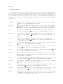
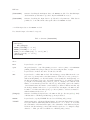
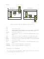
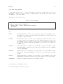
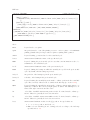
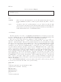
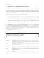
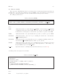
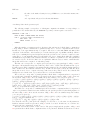
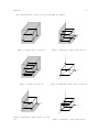
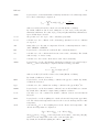
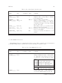
Presentation of fully- and partially-inserted 3-part control rods. . . . . . . . . . . .
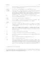
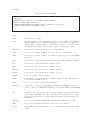
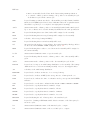
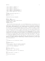
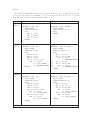
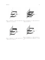
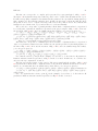
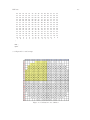
Complete grid, one point case . . . . . . . . . . . . . . . . . . . . . . . . . . . . . .
Complete grid, TA case . . . . . . . . . . . . . . . . . . . . . . . . . . . . . . . . .
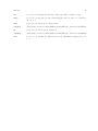
Partial grid, complete planes, one point case . . . . . . . . . . . . . . . . . . . . . .
Partial grid, complete planes, TA case . . . . . . . . . . . . . . . . . . . . . . . . .
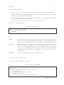
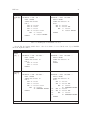
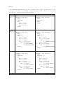
Partial grid, complete axis, one point case . . . . . . . . . . . . . . . . . . . . . . .
Partial grid, complete axis, TA case . . . . . . . . . . . . . . . . . . . . . . . . . .
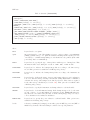
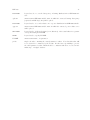
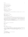
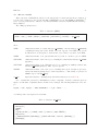
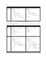
Partial grid, complete axis with another configuration, one point case . . . . . . .
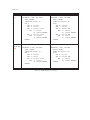
Partial grid, one complete plane and one complete axis, one point case . . . . . . .
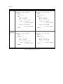
Partial grid, one complete plane and one complete axis, TA case . . . . . . . . . .
Partial grid, one complete plane and one complete axis with another configuration,
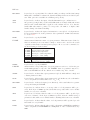
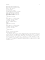
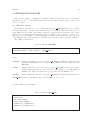
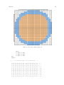
Face View of ACR Benchmark Core Model (292 Channels) . . . . . . . . . . . . .
Geometry definition (plane-1) . . . . . . . . . . . . . . . . . . . . . . . . . . . . . .
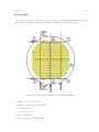
Top View of ACR Benchmark Core Model . . . . . . . . . . . . . . . . . . . . . . .
Combustion zones definition . . . . . . . . . . . . . . . . . . . . . . . . . . . . . . .
. . . . 18
. . . . 73
. . . . 73
. . . . 73
. . . . 73
. . . . 73
. . . . 73
. . . . 74
. . . . 74
. . . . 74
one point case 74
. . . . 132
. . . . 141
. . . . 144
. . . . 155
IGE–300
1
1 INTRODUCTION
DONJON is a full-core modelization code designed around solution techniques of the neutron diffusion
or simplified Pn equation.[1] The current DONJON package is an evolution version, released as an attempt
to introduce the innovative capabilities for the full-core modeling and simulations of different types of
nuclear reactors sush as Pressurized Water Reactors (PWRs), legacy CANDU reactors, and Advanced
CANDU Reactors (ACRs). The computer code DONJON (Release 4.0) is part of Version4 distribution[2] ,
built around the GAN generalized driver[3] . Its execution depends on other computer codes, components
of Version4, namely: GANLIB, UTILIB, DRAGON[4] , and TRIVAC[5] codes. The DRAGON modules are
used with DONJON code to define the reactor geometry, to provide the macroscopic cross-section libraries
and to perform micro-depletion calculations. The TRIVAC solver modules are used to perform a spatial
discretization of the reactor geometry and to provide the numerical solution according to the user-selected
numerical procedure[6–11] . The UTILIB library provides the utility and linear algebra libraries. Finally,
the GANLIB computer code provides CLE-2000 capabilities to control data flows and to implement
computational schemes. GANLIB also provide LCM data structures to exchange information between
modules.
The DONJON code is divided into several modules, each module is designed to perform some particular tasks. The transfer of information between the modules is achieved by means of well defined data
structure. Several design features, data structure and computing algorithms were recovered, revised and
adapted from the previous DONJON version[12, 13] . One of the main concerns of the DONJON developers
is to ensure the code reliability and extensibility.
The DONJON modules are first designed for the reactor full-core modeling in 3-D Cartesian geometry.
These modules are built around the reactor fuel lattice specification corresponding to the common design
features of CANDU reactors. The modules related to the modeling of reactivity mechanisms, which are
normally presented in the reactor core, also constitute an important part of code. The DONJON code can
perform several full-core calculations and can be used to determine some important core characteristics,
such as the power and normalized flux distributions over the reactor core. All full-core calculations using
current version of DONJON correspond to the reactor static conditions.
The modeling of the reactor fuel lattice using DONJON is made in considering that the fuel lattice is
composed of a well defined number of fuel channels and bundles. All reactor channels contain the same
number of fuel bundles and are identified by their specific names. The fuel bundles have a distinct set
of properties that are recovered and interpolated according to the specified global and local parameters.
The interpolation of fuel properties with respect to burnup distribution can be performed according to
the time-average or instantaneous models[14] . The time-average calculation is performed in considering
the bidirectional refuelling scheme of reactor channels and assuming that all channels have the same
bundle-shift.
The modeling of the reactivity mechanisms is based on their specified parameters, which include the
devices position, rods insertion level, water filling level, direction of movement, etc. The rod-devices
insertion level can be set according to their nominal positions or they can be displaced in and out of core.
The devices can also be divided into several groups so that they can be manipulated, displaced or moved
simultaneously. The time-dependent behaviour of the moving devices can be modeled and used for the
transient simulations or reactor control studies. The reactivity worth of devices can also be studied and
predicted using DONJON.
The reactor material properties are essentially recovered from the reactor database, obtained from
the lattice calculations using DRAGON code. The two distinct macroscopic cross-section libraries can be
constructed using DONJON. The first macrolib is constructed only for the material properties which
are evolution-independent, such as reflector and devices properties. The second macrolib is constructed
only for the fuel properties, defined per each fuel bundle over the fuel lattice. The two libraries are next
combined and updated, according to the devices insertion level. The produced extended macrolib is
subsequently used to obtain the numerical solution, using TRIVAC modules.
Finally, it should be noted that the DONJON code development is permanently in progress. The
future updates will provide several extended capabilities for the reactor design and calculations; they will
IGE–300
be gradually added to the subsequent DONJON versions.
2
IGE–300
3
2 GENERAL SPECIFICATION OF DONJON
2.1
Modules
Reactor calculations using DONJON are performed by means of sequential execution of several userselected modules, according to the user-defined computing scheme. Each module is designed to perform
some particular tasks. The detailed description of DONJON modules is given in Section 3 to Section 6.
In order to perform the reactor calculations, it is also required to use some DRAGON and TRIVAC
modules. For more details on DRAGON modules specification, refer to its user guide[4] ; for more details
on TRIVAC modules specification, refer to its user guide[5] . Because the code execution is controlled by
the GAN generalized driver, it is also possible to use its utility modules[3, 4] . A brief description of each
module that can be executed using DONJON is given below. A short description of each data structure
that can be used in DONJON is given in Section 2.2.
• The following DRAGON modules can be executed using DONJON:
GEO:
module used to create or modify a reactor geometry. The spatial locations of the
reactor material mixtures must also be defined using the GEO: module. Only 3-D
Cartesian reactor geometries are allowed with DONJON.
MAC:
module used to create or modify a macrolib containing the material properties, by
directly specifying the group-ordered macroscopic cross-sections for each selected material mixture.
• The following TRIVAC modules can be executed using DONJON:
TRIVAT:
module used to perform a 3-D numerical discretization or “tracking” of the reactor
geometry.
TRIVAA:
module used to compute the set of system matrices with respect to the previously
obtained ”tracking” information.
FLUD:
module used to compute the numerical solution to an eigenvalue problem, corresponding to a previously obtained set of system matrices.
• The following are short descriptions of utility modules that can be executed using DONJON:
UTL:
module used to perform several utility actions on a data structure.
DELETE:
module used to delete one or many data structures.
GREP:
module used to extract a single value from a data structure.
END:
module used to delete all the local linked lists, to close all the remaining local files and
to return from a procedure; or to terminate the overall DONJON execution controlled
by the GAN generalized driver.
• The following are short descriptions of DONJON modules:
IGE–300
4
CRE:
module used to create a macrolib containing the material properties, by interpolating
the nuclear properties from a mono-parameter database, previously generated in the
lattice code.
NCR:
module used to create a microlib or a macrolib containing the material properties,
by interpolating the nuclear properties from a multi-parameter database, previously
generated in the lattice code.
AFM:
module used to create a macrolib containing the material properties, by interpolating
the nuclear properties from a multi-parameter feedback model database, previously
generated in the lattice code.
USPLIT:
module used to create an extended reactor material index over the whole mesh-splitted
reactor geometry.
RESINI:
module used to define the fuel lattice, to create the fuel-map geometry and to specify
the global and local parameters.
MACINI:
module used to create an extended macrolib, in which the properties are stored per
each material region, over the whole mesh-splitted reactor geometry.
DEVINI:
module used for 3-D modeling of rod-type devices in the reactor core.
DETINI:
module used to read and store detector information.
LZC:
module used for 3-D modeling of liquid zone controllers in the reactor core.
DSET:
module used to set the new devices parameters, that can be used for the reactivity
worth studies.
MOVDEV:
module used to compute the time-dependent positions of the moving rod-type devices.
NEWMAC:
module used to create an extended macrolib, that will contain the updated material
properties, computed with respect to the actual devices positions.
FLPOW:
module used to compute and print powers and normalized fluxes over the reactor core.
TAVG:
module used to perform burnups calculation according to the time-average model,
compute burnups integration limits, core-average exit burnup, axial power-shapes and
channel refuelling rates.
TINST:
module used to perform burnups calculation according to the time-linear model and
compute instantaneous burnups values. This module is specific to Candu reactor
refuelling.
SIM:
module used to perform burnups calculation according to the time-linear model and
compute instantaneous burnups values. This module is specific to PWR reactor refuelling.
DETECT:
module used to compute the mean flux at each detector site and the response of each
detector according to different types of interpolation.
CVR:
module used for the core-voiding simulations.
HST:
module used to manage a full reactor execution in DONJON using explicit DRAGON
calculations for each cell (see Section 3.17).[18]
IGE–300
2.2
5
Data structures
The transfer of information between the modules is performed by means of well defined data structures, also called objects. The objects can be defined in either create, read-only or modification mode.
Each object has its own specific signature that can be easily recognized by a module. A detailed description of DONJON data structures is given in Section 7. For more details on DRAGON and TRIVAC data
structures, refer to their guide[17] . A brief description of all data structures that can be used in DONJON
is given below.
geometry
data structure containing the geometry information. This object has a signature
L GEOM; it is created using DRAGON module GEO:.
macrolib
data structure containing the multigroup macroscopic properties; it has a signature
L MACROLIB. This object can be created in several modules, namely: using DRAGON
modules MAC: and NCR:; or using DONJON modules CRE:, MACINI:, and NEWMAC:.
compo
data structure containing the mono-parameter database, generated by the lattice code.
This object has a signature L COMPO; it is created using DRAGON module CPO:.
multicompo
data structure containing the multi-parameter database, generated by the lattice code.
This object has a signature L MULTICOMPO; it is created using DRAGON module
COMPO:.
saphyb
data structure containing the multi-parameter database, generated by the lattice code.
This object has a signature L SAPHYB; it is created using the APOLLO2 lattice code
or the DRAGON module SAP:.
fmap
data structure containing the fuel-lattice specification. This object has a signature
L MAP; it is created using DONJON module RESINI:.
matex
data structure containing the extended reactor material index. This object has a
signature L MATEX; it is created using DONJON module USPLIT:.
device
data structure containing the devices specification. This object has a signature L DEVICE;
it is created using DONJON module DEVINI:.
detect
data structure containing detector positions and responses. This object has a signature
L DETECT; it is created using DONJON module DETINI:, and can be modified by the
modules DETINI: and DETECT: .
track
data structure containing a ”tracking” information of the reactor geometry. This
object has a signature L TRACK; it is created using TRIVAC module TRIVAT:.
system
data structure containing a set of system matrices. This object has a signature
L SYSTEM; it is created using TRIVAC module TRIVAA:.
flux
data structure containing the numerical solution to an eigenvalue problem. This object
has a signature L FLUX; it is created using TRIVAC module FLUD:.
power
data structure containing the powers and normalized fluxes over the reactor core. This
object has a signature L POWER; it is created using DONJON module FLPOW:.
history
This data structure contains the information required to ensure a smooth coupling
of DRAGON with DONJON when an history based full reactor calculation is to be
performed. It is used only by the HST: module.
IGE–300
2.3
6
Syntactic rules for input specification
The input data to any module is read in free format using the subroutine REDGET. CLE-2000 variables[21, 22]
are also allowed. The user guide for DONJON is written using the following convention:
• the parameters surrounded by single square brackets ‘[ ]’ denote an optional input;
• the parameters surrounded by double square brackets ‘[[ ]]’ denote an input which may be repeated
as many times as needed;
• the parameters in braces separated by vertical bars ‘{ | | }’ denote a choice where one and only one
input is mandatory;
• the parameters in bold face and in brackets ‘( )’ denote an input structure;
• the parameters in italics and in brackets with an index ‘(data(i) , i = 1, n )’ denote a set of n inputs;
• the words using the typewriter font KEYWORD are character constants used as keywords;
• the words in italics denote the user-defined variables: they are lower-case and of integer type (when
starting from i to n), or of real type (when starting from a to h or from o to z); or they are upper-case
and of character type CHARACTER.
2.4
General input structure
DONJON is built around the GAN generalized driver[3, 22] . Accordingly, all the modules that will be
used during the current execution must be first identified. It is also necessary to define the format of
each object (data structure) that will be processed by these modules. Then, the modules required for the
specific DONJON calculation are called successively, information being transferred from one module to
the next via the objects. Finally, the execution of DONJON is terminated when it encounters the END:
module, even if it is followed by additional data records in the input data stream. The general input data
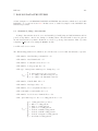
structure therefore follows the calling specifications given below:
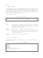
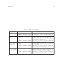
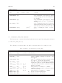
Table 1: Structure (DONJON)
[ MODULE [[ MODNAME ]] ; ]
[ LINKED LIST [[ STRNAME ]] ; ]
[ XSM FILE [[ STRNAME ]] ; ]
[ SEQ BINARY [[ STRNAME ]] ; ]
[ SEQ ASCII [[ STRNAME ]] ; ]
[[ (module) ; ]]
END: ;
where
MODULE
keyword used to specify the names of all modules that will be used in the current
DONJON execution.
MODNAME
character*12 name of a DONJON, or DRAGON, or TRIVAC, or utility module. The
list of modules that can be executed using DONJON code is provided in Section 2.1.
IGE–300
7
LINKED LIST
keyword used to specify the names of data structure that will be stored as linked lists.
XSM FILE
keyword used to specify the names of all data structure that will be stored on XSM
format files.
SEQ BINARY
keyword used to specify the names of all data structure that will be stored on sequential
binary files.
SEQ ASCII
keyword used to specify the names of all data structures that will be stored on sequential ASCII files.
STRNAME
character*12 name of a data structure. The list of data structure that can be used
in DONJON is presented in Section 2.2.
(module)
input specification for a module that will be executed. For DONJON specific modules,
these input structures are described in Section 3 to Section 6.
END:
keyword to call the normal end-of-execution utility module.
;
keyword to specify the end of record. This keyword is used to delimit the part of the
input data stream associated with each module.
Generally, the user has the choice to declare the most of data structure in the format of a linked list
to reduce CPU times or as a XSM file to reduce memory resources. In general, the data structure are
stored on the sequential ASCII files only for the backup purposes.
The input data normally ends with a call to the END: module. However, the GAN driver will insert
automatically the END: module, even if it was not provided, upon reaching an end-of-file in the input
stream.
Each (module) calling specification contains a module execution description and its associated input
structure. All these modules, except the END: module may be called more than once.
IGE–300
8
3 GENERAL CORE-DESCRIPTION MODULES
3.1
The RESINI: module
The RESINI: module is used for modeling of the reactor fuel lattice in 3-D Cartesian geometry or 3-D
Hexagonal geometry. This modeling is based on the following considerations:
• For 3-D Cartesian geometry, the reactor fuel lattice is composed of a well defined number of fuel
channels. Each channel is composed of a well defined number of fuel bundles or assembly subdivisions. All channels contain the same number of fuel bundles or assembly subdivisions. Each reactor
channel is identified by its specific name which corresponds to its position in the fuel lattice.
In a Candu reactor, the channels are refuelled according to the bidirectional refuelling scheme. The
refuelling scheme of a channel corresponds to the number of displaced fuel bundles (bundle-shift)
during each channel refuelling. The direction of refuelling corresponds to the direction of coolant
flow along the channel.
In a PWR, a basic assembly layout can be projected over the fuel map using a naval-coordinate
position system. Assembly refuelling and shuffling will be possible using the ad hoc module SIM:
(see Section 3.13).
• For 3-D Hexagonal geometry, the reactor fuel lattice is composed of a well defined number of fuel
channels and each channel is composed of a well defined number of fuel bundle. All fuel bundles
have the same volume. All channels contain the same number of fuel bundles. Refuelling is not
available during the calculation. The lattice indexation is kept to identify the hexagons.
• The fuel regions generally have a different set of global and local parameters. For example, the fuel
bundles have a different evolution of the fuel properties according to the given burnup distribution,
which is a global parameter. Consequently, the homogenized cell properties will differ from one
fuel region to another, i.e., they are not uniform over the fuel lattice. Thus, the realistic modeling
of a reactor core requires the fuel properties to be interpolated with respect to global and local
parameters, which must be specified in the fuel map.
Note that the above considerations correspond to the typical core modeling of CANDU or PWR reactors.
The RESINI: module will create a new FMAP object that will store the information related to the fuel
lattice specification and properties (see Section 7.1).
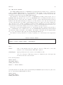
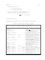
The RESINI: module specifications are:
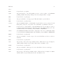
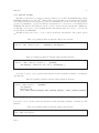
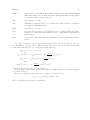
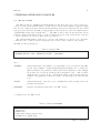
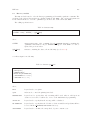
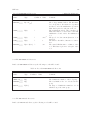
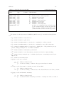
Table 2: Structure RESINI:
{ FLMAP MATEX := RESINI: MATEX :: (descresini1) |
FLMAP := RESINI: FLMAP :: (descresini2) }
where
FLMAP
character*12 name of the resini object that will contain the fuel-lattice information.
If FLMAP appears on both LHS and RHS, it will be updated; otherwise, it is created.
MATEX
character*12 name of the matex object specified in the modification mode. MATEX
is required only when FLMAP is created.
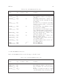
IGE–300
9
(descresini1)
structure describing the main input data to the RESINI: module. Note that this input
data is mandatory and must be specified only when FLMAP is created.
(descresini2)
structure describing the input data for global and local parameters. This data is
permitted to be modified in the subsequent calls to the RESINI: module.
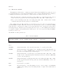
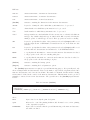
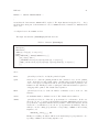
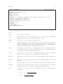
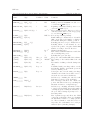
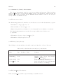
3.1.1 Main input data to the RESINI: module
Note that the input order must be respected.
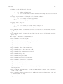
Table 3: Structure (descresini1)
[ EDIT iprint ]
::: GEO: (descgeo)
NXNAME ( XNAME(i) , i = 1, nx )
NYNAME ( YNAME(i) , i = 1, ny )
NCOMB { ncomb B-ZONE (icz(i) , i = 1, nch ) | ALL }
[ SIM lx ly (naval(i) , i = 1, nch ) ]
(descresini2)
where
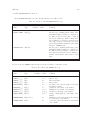
EDIT
keyword used to set iprint.
iprint
integer index used to control the printing on screen: = 0 for no print; = 1 for minimum
printing (default value); larger values produce increasing amounts of output.
:::
keyword used to indicate the call to an embedded module.
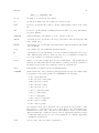
GEO:
keyword used to call the GEO: module. The fuel-map geometry differs from the complete reactor geometry in the sense that it must be defined as a coarse geometry, i.e.
without mesh-splitting over the fuel bundles. Consequently, the mesh-spacings over
the fuel regions must correspond to the bundle dimensions (e.g. hx =width; hy =height;
hz =length or in 3-D Hexagonal geometry hx =side; hz =height). Note that the total
number of non-virtual regions in the embedded geometry must equal to the number
of fuel channels times the number of fuel bundles per channel. This means that only
the fuel-type mixture indices are to be provided in the data input to the GEO: module
for MIX record. Other material regions (e.g. reflector) must be declared as virtual, i.e.
with the mixtures indices set to 0.
(descgeo)
structure describing the input data to the GEO: module (see the user guide[4] ). Only
3-D Cartesian or 3-D Hexagonal fuel-map geometry is allowed.
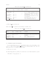
NXNAME
keyword used to specify XNAME. Not used for 3-D Hexagonal geometry.
XNAME
character*2 array of horizontal channel names. A horizontal channel name is identified by the channel column using numerical characters ’1’, ’2’, ’3’, and so on. Note that
the total number of X-names must equal to the total number of subdivisions along the
X-direction in the fuel-map geometry. All non-fuel regions are to be assigned a single
character ’-’. This option is not available for 3-D Hexagonal geometry.
IGE–300
10
nx
integer total number of subdivisions along the X-direction in the fuel-map geometry.
Not used for 3-D Hexagonal geometry.
NYNAME
keyword used to specify YNAME. Not used for 3-D Hexagonal geometry.
YNAME
character*2 array of vertical channel names. A vertical channel name is identified
by the channel row using alphabetical letters ’A’ (from the top), ’B’, ’C’, and so on.
The total number of Y-names must equal to the total number of subdivisions along
the Y-direction in the fuel-map geometry. All non-fuel regions are to be assigned a
single character ’-’. This option is not available for 3-D Hexagonal geometry.
ny
integer total number of subdivisions along the Y-direction in the fuel-map geometry.
Not used for 3-D Hexagonal geometry.
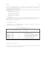
NCOMB
keyword used to specify the number of combustion zones.
ncomb
integer total number of combustion zones. This value must be greater than (or equal
to) 1 and less than (or equal to) the total number of reactor channels.
B-ZONE
keyword used to specify icz.
icz
integer array of combustion-zone indices, specified for every channel. A reactor channel
can belong to only one combustion zone, however a combustion zone can be specified
for several channels.
ALL
keyword used to indicate that the total number of combustion zones equals to the
number of reactor channels. In this particular case, each channel will have a unique
combustion-zone number. Hence, an explicit specification of the combustion-zone indices can be omitted.
nch
Nch : number of fuel channels in the radial plane.
nb
Nb : number of fuel bundles or assembly subdivisions in the axial plane.
SIM
keyword used to specify a basic assembly layout for the SIM: PWR refuelling module
(see Section 3.13).
lx
number of assemblies along the X axis. Typical values are 15 or 17.
ly
number of assemblies along the Y axis.
naval
character*3 identification name corresponding to the basic naval-coordinate position
of an assembly. naval(i) is the concatenation of a letter (generally chosen between A and
T) and of an integer (generally chosen between 01 and 17). An assembly may occupies
four positions in the fuel map in order to be represented by four radial burnups. In
this case, the same naval-coordinate value will appear at four different (i) indices.
3.1.2 Input of global and local parameters
The information with respect to the fuel burnup is required for the fuel-map macrolib construction,
using either the CRE:, NCR: or AFM: module. The fuel-region properties related to other local or global
parameters can be interpolated only using the NCR: module.
IGE–300
11
Table 4: Structure (descresini2)
[ EDIT iprint ]
[ BTYPE { TIMAV-BURN | INST-BURN } ]
[ TIMAV-BVAL (bvalue(i) , i = 1, ncomb ) ]
[ INST-BVAL { SAME bvalue | CHAN (bvalue(i) , i = 1, nch ) | BUND (bvalue(i) , i = 1, nch·nb ) |
SMOOTH } ]
[ BUNDLE-POW { SAME bvalue | CHAN (bvalue(i) , i = 1, nch ) | BUND (bvalue(i) , i = 1, nch·nb ) } ]
[ REF-SHIFT { ishift | COMB (ishift(i) , i = 1, ncomb ) } ]
[[ ADD-PARAM PNAME PNAME PARKEY PARKEY { GLOBAL | LOCAL } ]]
[[ SET-PARAM PNAME { pvalue | { [ TIMES PNAMEREF ] SAME pvalue |
CHAN (pvalue(i) , i = 1, nch ) | BUND (pvalue(i) , i = 1, nch·nb ) } } ]]
[[ FUEL { WEIGHT | ENRICH | POISON } (fvalue(i) , i = 1, nfuel ) ]]
[ CELL (ialch(i) , i = 1, nch ) ]
;
where
EDIT
keyword used to set iprint.
iprint
integer index used to control the printing on screen: = 0 for no print; = 1 for minimum
printing (default value); = 2 to print the channels refuelling schemes (if they are new
or modified); = 3 initial burnup limits per each channel are also printed (if the axial
power-shape has been reinitialized).
BTYPE
keyword used to specify the type of interpolation with respect to burnup data. This
information will be used during the execution of CRE:, NCR: or AFM: module.
TIMAV-BURN
keyword used to indicate the burnups interpolation according to the time-average
model. This option is not available in 3-D Hexagonal geometry.
INST-BURN
keyword used to indicate the burnups interpolation according to the instantaneous
model.
TIMAV-BVAL
keyword used to indicate the input of average exit burnup values per each combustion
zone. Note that the axial power-shape and the first burnup limits will be reinitialized
each time the average exit burnups are modified by the user. These data are required
for the time-average calculation (see Section 3.11). This option is not available with
3-D Hexagonal geometry.
INST-BVAL
keyword used to specify the instantaneous burnup values for each fuel bundle.
SMOOTH
keyword used to level fuel mixtures burnup. If the burnup is supposed to be the same
at each occurence of every fuel mixture (for symetry reasons), SMOOTH will make sure
they share the exact same value (the first one in the burnup map). Purpose is only to
correct calculation noise in historic calculation.
BUNDLE-POW
keyword used to specify the power values for each fuel bundle. This option is not
available in 3-D Hexagonal geometry.
bvalue
real array containing the burnups/powers values, given in MW·day per tonne/MW of
initial heavy elements. The fuel burnup is considered as a global parameter.
IGE–300
12
REF-SHIFT
keyword used to specify ishift. Note that the axial power-shape and the first burnup
limits will be reinitialized each time the channel refuelling schemes are modified by the
user. This option is not avaialble in 3-D Hexagonal geometry.
COMB
keyword used to indicate the input of bundle-shift numbers per combustion zone.
ishift
integer array (or single value) of the bundle-shift numbers. A single ishift value means
that the same bundle-shift will be applied for all combustion zones. Note that the
bundle-shift value must be positive, it corresponds to the number of displaced fuel
bundles during each channel refuelling.
ADD-PARAM
keyword used to indicate the input of information for a new global or local parameter.
For more information about the parameter data organization on FMAP data structure
see Section 7.1.5.
PNAME
keyword used to specify PNAME.
PNAME
character*12 identification name of a given parameter. This name is user-defined so
that it is arbitrary, however it must be unique so that it can be used for the search
of parameter information and interpolation purpose. Moreover, it is recommended to
use the following pre-defined values:
C-BORE Boron concentration
T-FUEL Averaged fuel temperature
T-SURF Surfacic fuel temperature
T-COOL Averaged coolant temperature
D-COOL Averaged coolant density
CANDU-only parameters:
T-MODE Averaged moderator temperature
D-MODE Averaged moderator density
PARKEY
keyword used to specify PARKEY .
PARKEY
character*12 corresponding name of a given parameter as it is recorded in the particular multi-parameter compo file. The PARKEY name of a parameter may not be
same as its PNAME and can also differ from one multi-compo file to another.
GLOBAL
keyword used to indicate that a given parameter is global, which will have a single and
constant parameter’s value.
LOCAL
keyword used to indicate that a given parameter is local. In this case, the total number
of recorded parameter’s values will be set to Nch × Nb .
SET-PARAM
keyword used to indicate the input (or modification) of the actual values for a parameter specified using its PNAME.
SAME
keyword used to indicate that a core-average value of a local parameter will be provided. If the keyword SAME is specified, then this average value will be set for all fuel
bundles for every reactor channel.
CHAN
keyword used to indicate that the values of a local parameter will be provided per
each reactor channel. If the keyword CHAN is specified, then the channel-averaged
parameter’s value will be set for all fuel bundles containing in the same reactor channel.
BUND
keyword used to indicate that the values of a local parameter will be specified per each
fuel bundle for every channel.
TIMES
keyword used to indicate that the values of the local parameter PNAME is a translation
of the local parameter PNAMEREF via a multiplication of the constant indicated by
SAME.
IGE–300
13
PNAMEREF
character*12 identification name of a given parameter.
pvalue
real array (or a single value) containing the actual parameter’s values. Note that these
values will not be checked for consistency by the module. It is the user responsibility
to provide the valid parameter’s values which should be consistent with those recorded
in the multicompo database.
FUEL
keyword used to indicate the input of data which will be specified for each fuel type.
WEIGHT
keyword used to indicate the input of fuel weight in a bundle, given in kg.
ENRICH
keyword used to indicate the input of fuel enrichment values, given in wt%.
POISON
keyword used to indicate the input of poison load in a fuel.
fvalue
real value of the fuel-type parameter, specified for each fuel type in the same order as
the fuel mixture indices have been recorded in the matex object (see Section 3.2.1).
nfuel
integer total number of the fuel types, as been defined in the USPLIT: module.
CELL
keyword used to specify that a patterned age distribution will be input and used to
compute instantaneous bundle burnup.
ialch
real array containing the refueling sequence numbers. This channel is refueled the
ialch(i)th one. The channels are ordering from the top left to the bottom right of the
core. The expression of the resulting bundle burnups are given in Ref. 19.
IGE–300
3.2
14
The USPLIT: module
The USPLIT: module is used to create a MATEX object that will provide a link between the reactor
geometry and material index. The 3-D Cartesian or 3-D Hexagonal reactor geometry, which is previously
produced in the GEO: module, is analyzed and the material mixture indices are recomputed in order to
provide a unique mixture number for each material sub-volume. Such renumbering permits a complex
reactor core modeling. A MATEX object is also used to store some additional information that will be
required and updated by other DONJON modules (see Section 7.2).
The USPLIT: module specification is:
Table 5: Structure USPLIT:
GEOM MATEX := USPLIT: { GEOM | GEOMOLD } :: (desclink)
where
GEOM
character*12 name of a geometry object. This object is defined in creation (appears
only on LHS) or modification (appears on both LHS and RHS) mode. An existing
geometry previously created in the GEO: module is modified. Only 3-D Cartesian or
3-D Hexagonal reactor geometries are allowed.
MATEX
character*12 name of a matex object to be created by the module.
GEOMOLD
character*12 name of a geometry object previously created in the GEO: module.
This object must be specified in read-only mode (appears only on RHS). It is copied
into GEOM at the beginning of USPLIT: module. Only 3-D Cartesian or 3-D Hexagonal reactor geometries are allowed.
(desclink)
structure describing the input data to the USPLIT: module.
3.2.1 Input data to the USPLIT: module
Note that the fuel-type and reflector-type mixture indices are need to be specified explicitly and the input
order must be respected.
Table 6: Structure (desclink)
[ EDIT iprint ]
NGRP ngrp
MAXR maxreg
NMIX nmixt
[ NREFL nrefl RMIX ( mixr(i) , i = 1, nrefl ) ]
[ NFUEL nfuel FMIX ( mixf (i) , i = 1, nfuel ) ]
;
IGE–300
15
where
EDIT
keyword used to set iprint.
iprint
integer index used to control the printing on screen: = 0 for no print; = 1 for minimum
printing (default value); larger values produce increasing amounts of output.
NGRP
keyword used to specify ngrp.
ngrp
integer total number of energy groups. This value must be greater than 0.
MAXR
keyword used to specify maxreg.
maxreg
integer maximum number of mesh-splitted regions in the reactor geometry. In 3-D
Hezagonal geometry, it corresponds to the total number of prismatic blocks lh *lz .
NMIX
keyword used to extend number of material mixtures in case new fuels are going to
be inserted in the fuel map in upcoming fuel cycles. By default, nmixt is set to the
maximum mixture index in RHS geometry GEOM or GEOMOLD.
nmixt
the maximum fuel mixture index in the complete life of the reactor. This number must
be greater than the maximum mixture index in RHS geometry GEOM or GEOMOLD.
NREFL
keyword used to specify nrefl.
nrefl
integer total number of reflector types. A reactor should have at least one reflector
material.
RMIX
keyword used to specify mixr.
mixr
integer array of the reflector-type mixture indices. Each reflector type is assigned a
distinct mixture number as previously defined in the geometry object.
NFUEL
keyword used to specify nfuel.
nfuel
integer total number of fuel types. A reactor should have at least one fuel type.
FMIX
keyword used to specify mixf .
mixf
integer array of the fuel-type mixture indices. Each fuel type is assigned a distinct
mixture number as previously defined in the geometry object.
IGE–300
3.3
16
The MACINI: module
The MACINI: module is used to construct an extended macrolib, in which the properties are stored
per each material region over the whole mesh-splitted reactor geometry. This macrolib is obtained by
combining the material properties which are contained in the two distinct macrolib objects:
• The first macrolib contains the material properties which are evolution-independent, such as
reflector and device properties. It is created using either MAC:, CRE:, NCR: or AFM: module.
• The second is a fuel-map macrolib created using either CRE:, NCR: or AFM: module. It must
contain the interpolated fuel properties per each fuel bundle.
The resulting macrolib will contain the properties that are stored for each reactor material and per
each mesh-splitted volume. When the devices are not present in the reactor core, then the resulting
macrolib can be considered as a complete reactor macrolib and it can be directly used for the numerical solving. However, when the devices are inserted into the reactor core, the resulting macrolib is not
yet complete; it must be subsequently updated with respect to the device properties, using the NEWMAC:
module (see Section 3.9).
The MACINI: module specification is:
Table 7: Structure MACINI:
MACRO2 MATEX := MACINI: MATEX MACRO [ MACFL ] :: [ EDIT iprint ] ;
where
MACRO2
character*12 name of the extended macrolib to be created by the module.
MATEX
character*12 name of the matex object containing an extended material index over
the reactor geometry. MATEX must be specified in the modification mode; it will
store the recovered h-factors per each fuel region.
MACRO
character*12 name of a macrolib, created using either MAC:, CRE:, NCR: or AFM:
module, for the evolution-independent material properties (see structure (desccre1)
or refer to the user guide[4] ).
MACFL
character*12 name of a fuel-map macrolib, created using either CRE:, NCR: or AFM:
module, for the interpolated fuel properties (see structure (desccre2) or refer to the
user guide[4] ).
EDIT
keyword used to set iprint.
iprint
integer index used to control the printing on screen: = 0 for no print; = 1 for minimum
printing; larger values produce increasing amounts of output. The default value is
iprint = 1.
IGE–300
3.4
17
The DEVINI: module
The DEVINI: module is used for the modeling of reactivity mecanisms, based on the devices specifications which are read from the input data file. The module will create a new device object that will
store the devices specifications and parameters (see Section 7.3). Note that only the rod-type (i.e. solid)
devices are considered using the DEVINI: module; the liquid zone controllers can be added subsequently,
using the LZC: module (see Section 3.6). A rod-type device is a reactivity controller rod (or plate), such
as: a zone control rod (ZCR), a shutoff rod (SOR), etc. Several devices parameters can be modified using
the DSET: module (see Section 3.7).
A device specification includes several controller rod parameters, such as: a rod position, rod insertion level, direction of movement, etc. The devices positions can not overlap in the reactor core; they
are referred using 3-D-Cartesian coordinates. The insertion level of rods can be set according to their
nominal positions or they can be displaced in or out of core. The rods can also be divided into the several
user-defined groups so that they can be manipulated, displaced or moved simultaneously.
The DEVINI: module specification is:
Table 8: Structure DEVINI:
DEVICE MATEX := DEVINI: MATEX :: (descdev)
where
DEVICE
character*12 name of the device object that will be created by the module; it will
contain the devices information.
MATEX
character*12 name of the matex object that will be updated by the module. The
rod-devices material mixtures are appended to the previous material index and the
rod-devices indices are also modified, accordingly.
(descdev)
structure describing the input data to the DEVINI: module.
3.4.1 Input data to the DEVINI: module
The DEVINI: module allows the definition of rod-type devices made of one or many (up to 10) parts,
as depicted in Fig. 1.
Table 9: Structure (descdev)
[ EDIT iprint ]
NUM-ROD nrod [ { FADE | MOVE } ]
( (dev-rod), i = 1, nrod )
[ CREATE ROD-GR ngrp ( (rod-group), i = 1, ngrp ) ]
;
IGE–300
18
part 3
Upper insertion (H+)
Lower insertion (H−)
part 3
part 2
part 3
part 1
Lsup
(level) < 1
MOVE
part 2
(level) < 1
FADE
part 1
part 1
L1
(level) = 1
(level) = 1
(L2 -L1)x(level)
L2
(L2 -L1)x(level)
part 2
part 3
Lsup
(level) < 1 part 2
FADE
part 1
(level) < 1
MOVE
Figure 1: Presentation of fully- and partially-inserted 3-part control rods.
where
EDIT
keyword used to set iprint.
iprint
integer index used to control the printing on screen: = 0 for no print; = 1 for minimum
printing (default value); larger values produce increasing amounts of output.
NUM-ROD
keyword used to specify nrod.
nrod
integer total number of the reactor rod-type devices. This number must be greater
than 0.
FADE
fading rod keyword. A fraction of the fully inserted rod vanishes (default option).
MOVE
moving rod keyword. The complete rod is moving (DONJON3-type movement).
CREATE
keyword used to create the rod-groups of devices. The creation of groups is optional.
ROD-GR
keyword used to set ngrp.
ngrp
integer total number of the rod groups to be created. This number must be greater
than 0.
(dev-rod)
structure describing the input data for each individual rod.
(rod-group)
structure describing the input data for each group of rods.
3.4.2 Description of dev-rod input structure
A rod position is referred by its 3-D Cartesian coordinates only. Note that the devices positions can
not overlap. The input order of data must be respected.
IGE–300
19
Table 10: Structure (dev-rod)
ROD id
ROD-NAME NAME
AXIS { X | Y | Z }
FROM { H+ | H- }
[ LEVEL value ]
[ SPEED speed ]
[ TIME time ]
[[ MAXPOS (pos(i), i = 1, 6) DMIX mix1 mix2 ]]
ENDROD
where
ROD
keyword used to specify the rod id number.
id
integer identification number of the current rod. Each rod-type device must be assigned
a unique id number, given in an ascending order ranging from 1 to nrod.
ROD-NAME
keyword used to specify the rod NAME.
NAME
character*12 name of the current rod. In general, this name is composed by the rod
specific type (e.g. SOR, ZCR, etc.) followed by its sequential number (e.g. 01, 02,
etc.).
AXIS
keyword used to specify the rod movement axis. A rod can be displaced along only
one of the axis.
X
keyword used to specify that a rod is displaced along X axis.
Y
keyword used to specify that a rod is displaced along Y axis.
Z
keyword used to specify that a rod is displaced along Z axis.
FROM
keyword used to specify the insertion side of geometry. The rod-devices can be inserted
into the reactor core from only one side of geometry. For example, some vertically
moving devices can be inserted only from the top, whereas other only from the bottom.
H+
keyword used to specify that a rod will be inserted into reactor core from the highest
position (e.g. from the top for vertically moving rod-device).
H-
keyword used to specify that a rod will be inserted into reactor core from the lowest
position (e.g. from the bottom for vertically moving rod-device).
LEVEL
keyword used to specify the actual rod insertion level value. By default, the rod
insertion level is left undefined.
value
real positive value of the rod insertion level. This value is used to compute the actual
rod position in the reactor core. The rod insertion level is minimal (value = 0.0) when
the rod is completely withdrawn, and it is maximal (value = 1.0) when the rod is fully
inserted. For the partially inserted rod the insertion level must be: 0.0 < value < 1.0
SPEED
keyword used to specify speed. By default, the speed is left undefined.
speed
real positive value of the rod movement speed, given in cm/s. This value is needed
only for the reactor regulating purpose.
IGE–300
20
TIME
keyword used to specify time. By default, the insertion time is left undefined.
time
real value of time for the rod insertion (or extraction), given in sec. This value is
needed only for the reactor regulating purpose.
MAXPOS
keyword used to specify the full-inserted coordinates of a rod part. The sequence of
MAXPOS and DMIX data structures is repeated for each part making the rod.
pos
real array containing 3-D Cartesian coordinates of the full-inserted rod. This is the
limiting rod position in the reactor core, which may or may not be the same as the
actual rod position. These coordinates must be given in the order: X−, X+, Y−, Y+,
Z−, and Z+.
DMIX
keyword used to specify mix1 and mix2.
mix1
first of two integer rod mixture indices. Index mix1 corresponds to the perturbed cross
sections.
mix2
second of two integer rod mixture indices. Index mix2 corresponds to the reference
cross sections. Indices mix1 and mix2 will be used to compute the incremental cross
sections in the NEWMAC: module.
ENDROD
keyword used to end the rod description.
3.4.3 Description of rod-group input structure
The partition of devices into groups is very useful when the same action is to be applied to several rods,
e.g. setting of new parameters (using the DSET: module) or rods moving (using the MOVDEV: module).
Table 11: Structure (rod-group)
GROUP-ID igrp { ROD-ID [[ id ]] | ALL }
where
GROUP-ID
keyword used to set igrp number.
igrp
integer identification number of a group to be created. Each rods group must be
assigned a unique identification number, given in ascending order ranging from 1 to
ngrp.
ROD-ID
keyword used to set the rod id numbers.
id
integer identification numbers of rods which belong to the same group igrp. A particular rod (or several rods) may belong to different groups, but it could not be repeated
inside the same group. The total number of rods in any group must be between 1 and
nrod.
ALL
keyword used to specify that all rods will belong to the same group igrp.
IGE–300
3.5
21
The DETINI: module
The DETINI: module is used to read and store detector information. A detector is represented by a
2-D or 3-D Cartesian/Hexagonal geometry.
The DETINI: module specification is:
Table 12: Structure DETINI:
DETECT := DETINI: [ DETECT ] :: (descdet)
where
DETECT
character*12 name of the detect object that will be created by the module; it will
contain the detector informations. If detect appear on RHS, it is updated, otherwise,
it is created.
(descdev)
structure describing the input data to the DETINI: module.
3.5.1 Input data to the DETINI: module
Note that the input order must be respected.
Table 13: Structure (descinidet)
[ EDIT iprt ] [ HEXZ ] NGRP ngrp
[[ TYPE NAMTYP
INFO ndetect nrep { SPECTRAL ( spec(i), i=1,ngrp ) | DEFAULT }
[ INVCONST ( tinv(i), i=1,nrep−2 ) ] [ FRACTION ( fract(i), i=1,nrep−1 ) ]
( (descdet), i=1,ndetect ) ]]
;
where
EDIT
keyword used to set iprt.
iprt
index used to control the printing in module INIDET:. =1,2 for no print(default
value); =3 for printing the contents of the output detect.
HEXZ
keyword to specify that only hexagonal detectors will be defined. If this keyword is
absent, Cartesian detectors will be defined.
NGRP
keyword used to set ngrp.
ngrp
number of energy groups in the calculation. It must be equal to the number set in the
MACD: module or by the compo files.
IGE–300
22
TYPE
keyword to specify the detector type.
NAMTYP
character*12 name of the detector type. To correspond to the actual detector response model encoded, the type of detector must be in this list:
• PLATN REGUL
• PLATN SAU
• VANAD REGUL
• CHION SAU
• CHION REGUL
For other type names, only a fixed normalisation can be performed.
INFO
keyword to specify the information associated with the detector type.
ndetect
number of detectors of the specified type.
nrep
number of detector response components for the specified type. It must be greater or
equal to 2, corresponding to a response in fraction and the reference flux value.
SPECTRAL
keyword to specify the energy spectral of a detector type.
spec
array containing the energy spectral of a detector type.
DEFAULT
keyword to specify the energy spectral will be initialized as 1.0 for the highest energy
group and 0.0 for other groups.
INVCONST
keyword to specify the inverse time constants of the detector type model. This option
is only valid for platinum, (NAMTYP(1:5) = ’PLATN’), detector type.
tinv
array containing the inverse time constants of the detector model.
FRACTION
keyword to specify the fractions corresponding to each delayed or prompt reponse of
the detector type model. This option is only valid for platinum, (NAMTYP(1:5) =
’PLATN’), detector type.
frac
array containing the detector type model fractions.
(descdet)
structure describing the format used to read detector information.
3.5.2 Description of the detector data
Note that the information input order must be respected.
Table 14: Structure (descdet)
NAME NAMDET
[ NHEX nhex HEX ( ihex(i), i=1,nhex ) ]
POSITION ( pos(i), i=1,6 )
RESP ( rep(i), i=1,nrep )
ENDN
IGE–300
23
where
NAME
keyword to specify the detector name.
NAMDET
character*12 name of the detector. The different names in alphabetical order must
fit their usual numbering in the core.(Ex: PLATN01, CHION01C)
NHEX
keyword to set the number of hexagons where the detector is placed.
nhex
number of hexagons.
HEX
keyword to set the hexagon numbers corresponding to the detector position.
ihex
array containing the hexagon numbers where the detector is present, as ordered in the
geometry definition.
POSITION
keyword to specify the detector coordinates.
pos
array containing the positions of the specified detector. The positions must be read
as X− X+ Y− Y+ Z− Z+ . For 2-D geometry, Z coordinates must be 0.0 and a
value greater than 1.0. For hexagonal geometry, only Z coordinates are used in 3-D
representation.
RESP
keyword to specify the detector initial responses.
rep
array containing the initial responses of the detector. To use the current detector
models in DONJON, responses are given as
• For vanadium detectors: current response, last response.
• For platinum detectors: current response, reference flux, last detector slow responses.
• For ion chamber detectors: current logarithmic response, current log rate response, reference flux.
ENDN
keyword to specify the end of the detector informations.
IGE–300
3.6
24
The LZC: module
The LZC: module is used for the modeling of liquid zone controllers, which are normally presented
in the CANDU6-type reactor core. The liquid zone controllers specifications are read from the input
data file. Note that this modeling can be made after the rod-type devices have been previously defined
using the DEVINI: module (see Section 3.4). In this case, the previously created device object will be
updated by the LZC: module; it will store the additional and separate information with respect to the
liquid controllers (see Section 7.3).
The liquid zone controller specification includes several device parameters, such as: the whole device position, water filling level, direction of filling, etc. Note that a liquid zone controller is normally
composed of two parts: one part is empty and the second part is full-filled. The water level can be
adjusted according to the control reactivity requirements. The controllers positions are referred using
3-D-Cartesian coordinates. Several devices parameters can be modified using the DSET: module (see
Section 3.7). The liquid controllers can also be divided into the several user-defined groups so that they
can be manipulated simultaneously.
The LZC: module specification is:
Table 15: Structure LZC:
DEVICE MATEX := LZC: [ DEVICE ] MATEX :: (desclzc)
where
DEVICE
character*12 name of the device object. Note, if the rod-type devices are not
present in the reactor core, then DEVICE object must appear only on the LHS (i.e.
in create mode), it will contain the information only with respect to the liquid zone
controllers. However, if the rod-type devices are present in the reactor core, then they
must be specified first (i.e. before the liquid controllers) using the DEVINI: module
(see Section 3.4). In the last case, the DEVICE object must also appear on the RHS
(i.e. in modification mode), it will contain the additional and separate information
with respect to the liquid zone controllers.
MATEX
character*12 name of the matex object that will be updated by the module. The
lzc-devices material mixtures are appended to the previous material index and the
lzc-devices indices are also modified, accordingly.
(desclzc)
structure describing the input data to the LZC: module.
3.6.1 Input data to the LZC: module
Note that the input order must be respected.
IGE–300
25
Table 16: Structure (desclzc)
[ EDIT iprint ]
NUM-LZC nlzc
((dev-lzc), i = 1, nlzc)
[ CREATE LZC-GR ngrp ((lzc-group), i = 1, ngrp) ]
;
where
EDIT
keyword used to set iprint.
iprint
integer index used to control the printing on screen: = 0 for no print; = 1 for minimum
printing (default value); larger values produce increasing amounts of output.
NUM-LZC
keyword used to specify nlzc.
nlzc
integer total number of liquid zone controllers. This number must be greater than 0.
CREATE
keyword used to create the lzc-groups of devices. The creation of groups is optional.
LZC-GR
keyword used to set ngrp.
ngrp
integer total number of the lzc groups to be created. This number must be greater
than 0.
(dev-lzc)
structure describing the input data for each individual liquid controller.
(lzc-group)
structure describing the input data for each group of liquid controllers.
3.6.2 Description of dev-lzc input structure
Note that the devices positions can not overlap in the reactor core. The input order of data must be
respected.
Table 17: Structure (dev-lzc)
LZC id
MAXPOS ( pos(i) , i = 1, 6 )
MAX-FULL fmax
AXIS { X | Y | Z }
LEVEL value
[ RATE rate ]
[ TIME time ]
EMPTY-MIX ( mixE(n), n = 1, 2 )
FULL-MIX ( mixF(n), n = 1, 2 )
IGE–300
26
where
LZC
keyword used to specify the liquid controller id number.
id
integer identification number of the current liquid controller. Each controller must be
assigned a unique id number, given in an ascending order ranging from 1 to nlzc.
MAXPOS
keyword used to specify the entire position of a liquid zone controller, including its
empty and full parts.
pos
real array containing 3-D Cartesian coordinates of the liquid zone controller position
in the reactor core. These coordinates must be given in the order: X− X+ Y− Y+
Z− Z+
MAX-FULL
keyword used to specify fmax.
fmax
real value of the limiting coordinate along the controller filling axis, which corresponds
to the maximum full-filling level for the current liquid controller.
AXIS
keyword used to specify the controller filling axis. A liquid controller can be filled
along only one (vertical) axis.
X
keyword used to specify that a liquid controller is filled along X axis.
Y
keyword used to specify that a liquid controller is filled along Y axis.
Z
keyword used to specify that a liquid controller is filled along Z axis.
LEVEL
keyword used to specify the actual filling level.
value
real positive value of the water level. This value is minimal (value = 0.0) when the
controller is empty, and it is maximal (value = 1.0) when the controller is full-filled.
For the partially filled controller the water level must be: 0.0 < value < 1.0
RATE
keyword used to specify rate.
rate
real positive value of the water filling rate, given in m3 /s. This value is needed only
for the reactor regulating purpose.
TIME
keyword used to specify time.
time
real value of the filling time, given in sec. This value is needed only for the reactor
regulating purpose.
EMPTY-MIX
keyword used to specify mixE.
mixE
two integer mixture indices, specified for the empty-part of liquid controller. The first
and the second mixture indices correspond to the perturbed and the reference cross
sections, respectively. These indices will be used to compute the incremental cross
sections in the NEWMAC: module.
FULL-MIX
keyword used to specify mixF.
mixF
two integer mixture indices, specified for the full-part of liquid controller. The first
and the second mixture indices correspond to the perturbed and the reference cross
sections, respectively. These indices will be used to compute the incremental cross
sections in the NEWMAC: module.
IGE–300
27
3.6.3 Description of lzc-group input structure
The partition of lzc-devices into groups is similar to that of rod-devices.
Table 18: Structure (lzc-group)
GROUP-ID igrp { LZC-ID [[ id ]] | ALL }
where
GROUP-ID
keyword used to set igrp number.
igrp
integer identification number of a group to be created. Each controllers group must
be assigned a unique identification number, given in ascending order ranging from 1
to ngrp.
LZC-ID
keyword used to set the controllers id numbers.
id
integer identification numbers of the liquid controllers which belong to the same group
igrp. A particular controller (or several devices) may belong to different groups, but
it could not be repeated inside the same group. The total number of liquid controllers
in any group must be between 1 and nlzc.
ALL
keyword used to specify that all liquid controllers will belong to the same group igrp.
IGE–300
3.7
28
The DSET: module
The DSET: module is used to set or to update some of the devices parameters. The new parameters
can be applied for the rod-type devices and/or for the liquid zone controllers, such as: the new insertion level for the rods or water filling level for the lzc-type devices, etc. It is possible to apply the new
parameters to the individual user-selected devices as well as to the user-selected groups of devices. If
the device (rod-insertion or lzc-filling) level is selected for the modification, then a new device position
is recomputed accordingly. The DSET: module can be used to perform the device reactivity studies and
also to predict the reactivity worth of the rod-devices.
The DSET: module specification is:
Table 19: Structure DSET:
DEVICE := DSET: DEVICE :: (descdset)
where
DEVICE
character*12 name of the device object that will be updated by the module.
(descdset)
structure describing the input data to the DSET: module.
3.7.1 Input data to the DSET: module
It is possible to set or to modify the parameters for several individual devices and/or for several groups
of devices simultaneously.
Table 20: Structure (descdset)
EDIT iprint
[[ { ROD irod | ROD-GROUP irgrp | LZC ilzc | LZC-GROUP ilgrp }
[ LEVEL value ] [ SPEED speed ] [ TIME time ]
END ]]
;
where
EDIT
keyword used to set iprint.
iprint
integer index used to control the printing on screen: = 0 for no print; = 1 for minimum
printing; larger values produce increasing amounts of output.
ROD
keyword used to specify the rod irod number.
irod
integer identification number of a rod to be modified. Each rod-type device has a
IGE–300
29
unique irod number, ranging from 1 to nrod, as been defined in the DEVINI: module
(see Section 3.4.2).
ROD-GROUP
keyword used to specify the rod-group irgrp number.
irgrp
integer identification number of a rod-group of devices that will be modifed with the
same parameters. Each rod-group has a unique irgrp number, ranging from 1 to ngrp,
as been defined in the DEVINI: module (see Section 3.4.3).
LZC
keyword used to specify the liquid controller ilzc number.
ilzc
integer identification number of a liquid controller to be modified. Each lzc-type device
has a unique ilzc number, ranging from 1 to nlzc, as been defined in the LZC: module
(see Section 3.6.2).
LZC-GROUP
keyword used to specify the lzc-group ilgrp number.
ilgrp
integer identification number of a lzc-group of devices that will be modifed with the
same parameters. Each lzc-group has a unique ilgrp number, ranging from 1 to ngrp,
as been defined in the LZC: module (see Section 3.6.3).
LEVEL
keyword used to specify a new level value.
value
real positive value of the new device level. For the rod-type devices this value must
correspond to the new rod insertion level (see Section 3.4.3). For the lzc-type devices
this value must correspond to the new water filling level (see Section 3.6.2). In any
case, the new level value must be: 0.0 ≤ value ≤ 1.0
SPEED
keyword used to specify a new value for speed.
speed
real positive value of the device speed. For the rod-type devices this value must
correspond to the speed of rod movement (insertion or extraction), given in cm/s. For
the lzc-type devices this value must correspond to the water filling rate, given in m3 /s.
The value of speed is required only for the reactor regulating purpose.
TIME
keyword used to specify a new value for time.
time
real value of time either for the rod insertion (or extraction) or for the liquid controller
filling, given in sec. The value of time is required only for the reactor regulating
purpose.
END
keyword used to indicate the end of input of the new parameters for the current device
or group of devices.
IGE–300
3.8
30
The MOVDEV: module
The MOVDEV: module can be used for the transient simulations and reactor control studies, which are
related to the time-dependent rod-devices displacement in the reactor core. The rods can be inserted into
or extracted from the reactor core, at constant or at variable speed of movement. The rod positions are
recomputed at every given time step of movement. The new rod positions can be computed in several
ways, based on either: current time increment and movement speed; relative change in rod positions; or
current rod insertion level. The MOVDEV: module allows the rod-devices to be displaced individually or
simultaneously in groups.
The MOVDEV: module specification is:
Table 21: Structure MOVDEV:
DEVICE := MOVDEV: DEVICE :: (descmove)
where
DEVICE
character*12 name of the device object that will be modified by the module. The
rods positions are updated according to the current time step of movement.
(descmove)
structure describing the input data to the MOVDEV: module.
3.8.1 Input data to the MOVDEV: module
It is possible to move several individual rods and/or several groups of rods simultaneously. A user
must be aware that a particular device will not be displaced more than once during the same time step.
Note that the input order of data to the module must be respected.
Table 22: Structure (descmove)
[ EDIT iprint ]
DELT delt
[[ { ROD id | GROUP igrp }
{ INSR | EXTR }
{ LEVEL value | DELH delh | SPEED speed } ]]
;
where
EDIT
keyword used to set iprint.
iprint
integer index used to control the printing on screen: = 0 for no print; = 1 for minimum
printing (default value); larger values produce increasing amounts of output.
IGE–300
31
DELT
keyword used to set delt.
delt
real value of the time increment for the current time step, given in sec.
ROD
keyword used to specify the rod id number.
id
integer identification number of a rod-type device to be displaced. Each rod has a
unique id number, ranging from 1 to nrod, as been defined in the DEVINI: module
(see Section 3.4.2).
GROUP
keyword used to specify a rod-group igrp number.
igrp
integer number of a group of rods that will be displaced simultaneously, with the same
parameters of movement. Each group of rod-devices has a unique igrp number, ranging
from 1 to ngrp, as been defined in the DEVINI: module (see Section 3.4.3).
INSR
keyword used to specify that a particular rod or a group of rods will be inserted into
the reactor core during the period of time delt.
EXTR
keyword used to specify that a particular rod or a group of rods will be extracted from
the reactor core during the period of time delt.
LEVEL
keyword used to specify the new level value.
value
real positive value of the rod insertion level at current time step. This value will
be used to compute the new rod position in the reactor core. The insertion level is
minimal (value = 0.0) when the rod is completely withdrawn, and it is maximal (value
= 1.0) when the rod is fully inserted. For the partially inserted rod the insertion level
must be: 0.0 < value < 1.0
DELH
keyword used to specify the value delh.
delh
real positive (absolute) value of the relative change in the rod position during the period
of time delt. This is a time-dependent rod displacement along the rod movement axis,
which must be given in cm.
SPEED
keyword used to set the current value of speed.
speed
real positive (absolute) value of the rod movement speed, given in cm/s. The rod
speed can be kept constant or it can be modified at any time step delt. The devices
could also have the different speeds of movement.
IGE–300
3.9
32
The NEWMAC: module
The NEWMAC: module is used to create a complete macrolib with respect to the devices parameters.
The resulting macrolib will contain the exact properties for every material region, over the whole meshsplitted reactor geometry. The material properties of each region are recomputed with respect to the
actual position of each rod-type and if present lzc-type device. The computing algorithm is based on the
determination of the volumic fraction occupied by each device; the incremental cross sections are then
adjusted, accordingly. Note that the NEWMAC: module must be executed each time the devices positions
are modified from the previously computed ones.
The NEWMAC: module specification is:
Table 23: Structure NEWMAC:
MACRO3 MATEX := NEWMAC: MATEX MACRO2 DEVICE :: [ EDIT iprint ] [ XFAC xfac ] ;
where
MACRO3
character*12 name of the macrolib to be created by the module. It will contain
the updated properties of each material region with respect to the current position of
each device.
MATEX
character*12 name of the matex object, containing the complete reactor material
index including devices. MATEX must be specified in the modification mode; it will
store the updated h-factors, computed per each fuel region with respect to the devices
positions.
MACRO2
character*12 name of the read-only extended macrolib, previously created by the
MACINI: module.
DEVICE
character*12 name of the read-only device object containing the devices information
and parameters.
EDIT
keyword used to set iprint.
iprint
integer index used to control the printing on screen: = 0 for no print; = 1 for minimum
printing; larger values produce increasing amounts of output. The default value is
iprint = 1.
XFAC
keyword used to specify the number of cells on which incremental cross sections were
computed in the supercell code.
xfac
corrective factor for delta sigmas (real number). For DRAGON code, xfac is generally
set to 2.0 and, for MULTICELL code, set to 1.0 . The default value is 2.0.
IGE–300
3.10
33
The FLPOW: module
The FLPOW: module is used to compute and print the flux and power distributions over the reactor
core. It also computes and prints some additional information, for example: the fluxes ratios with respect
to the thermal energy-group fluxes; the mean power density; the power- and flux-form factors; etc. The
computed fluxes and powers are printed either on files or on the screen. Note that the calculation using
the FLPOW: module can be performed once the numerical solution has been previously established using
the FLUD: or KINSOL: module.
According to the user-selected module specification, the average fluxes and powers can be computed
per each fuel region over the fuel lattice and/or per each material region over the whole reactor geometry.
In either case, all fluxes are normalized to the given total reactor power corresponding to the reactor
nominal conditions at core equilibrium. If the reactor is perturbed from its initial state, then a new total
reactor power can be recomputed and, accordingly, the flux and power distributions will be updated using
the previously computed normalization factor.
The FLPOW: module will create a new POWER object that will store the information related to the
reactor fluxes and powers (see Section 7.5). In addition, the POWER object will store several parameters
that can be used as power and criticity constraints for the optimization and fuel management purposes,
namely: the maximum channel and bundle powers; the channel and bundle power-form factors; the effective multiplication factor (recovered from the flux or kinet data structure).
The FLPOW: module specifications are:
Table 24: Structure FLPOW:
{
POWER [ NRMFLUX ] [ FMAP ]
:= FLPOW: [ POWOLD ] FMAP { FLUX | KINET } TRACK MATEX
:: (descflpow)
|
POWER := FLPOW: [ POWOLD ] { FLUX | KINET } TRACK MACRO
:: (descflpow)
}
where
POWER
character*12 name of the power object that will be created by the module. It will
contain the information related to the reactor fluxes and powers.
NRMFLUX
character*12 name of the flux object, in creation mode. According to the chosen
option, this object contains either the fluxes normalized to the given total reactor
power or the fluxes per bundle. Is it useful if you want to compute the detectors
readings with the DETECT: module.
POWOLD
character*12 name of the read-only power object. It must contain the previously
computed flux normalization factor, which corresponds to the reactor nominal or equilibrium conditions.
FMAP
character*12 name of the fmap object containing the fuel lattice specification. When
FMAP is specified on the RHS, the fluxes and powers calculations are performed over
IGE–300
34
the fuel lattice as well as over the whole reactor geometry. If FMAP is specified on the
LHS, its records ’BUND-PW’ and ’FLUX-AV’ will be set according to the information
present in POWER.
FLUX
character*12 name of the flux object, previously created by the FLUD: module. The
numerical flux solution contained in FLUX is recovered and all flux are normalized to
the given total reactor power.
KINET
character*12 name of the kinet object, previously created by the KINSOL: module.
The numerical flux solution contained in KINET is recovered.
TRACK
character*12 name of the track object, created by the TRIVAT: module. The information stored in TRACK is recovered and used for the average flux calculation.
MATEX
character*12 name of the matex object, containing the reactor material index and
the h-factors that will be recovered and used for the power calculation.
MACRO
character*12 name of the macrolib object, containing the h-factors that will be
recovered and used for the power calculation.
(descflpow)
structure describing the input data to the FLPOW: module .
3.10.1 Input data to the FLPOW: module
Note that the fuel-lattice power distribution can be printed only on the screen.
Table 25: Structure (descflpow)
[
[
[
[
[
;
EDIT iprint ]
{ PTOT power | P-NEW } ]
FSTH fsth ] [ INIT ]
{ NORM | BUND } ]
PRINT { MAP | DISTR [ FLUX ] [ RATIO ] [ POWER ] | ALL } ]
where
EDIT
keyword used to set iprint.
iprint
integer index used to control the printing on screen: = 0 for no print; = 1 for minimum
editing (default value); = 2 only channel powers in radial plane are printed; = 3 only
bundle powers per each radial plane are printed; = 10 only bundle powers per each
channel are printed. Any combination of the values 2, 3 and 10 is possible, for example
5 = 2+3. Note that any other value of iprint behaves as the first lower possible value,
for example 7 gives the same output as 5. Moreover channel and bundle powers can
be printed only if the FMAP object was provided in the calling specification.
PTOT
keyword used to specify the input of power. By default, a power is recovered from the
KINET object.
IGE–300
35
power
real total reactor power, given in MW. This value must correspond to the reactor
nominal conditions.
FSTH
keyword to specify the thermal to fission power ratio.
fsth
thermal to fission power ratio. By default this value is not used, and the total power
is the one given after the PTOT keyword.
INIT
keyword used to save the actual power distribution in the BUND-PW-INI record of the
fuel map object FMAP. It is used by the AFM: module to apply power feedback during
a fast transient using the initial power distribution instead of the actual power.
P-NEW
keyword used to indicate that a new total reactor power is to be recomputed, based on
the previously calculated flux normalization factor. The flux and power distributions
over the reactor core are updated, accordingly. Note that this option is valid only if a
read-only POWOLD object is provided.
PRINT
keyword used to indicate the printing on files. Note that all produced files will have
the same extension “.res”.
MAP
keyword used to specify the printing of the average fluxes and flux ratios per fuel
bundle. The normalized bundle fluxes are computed and printed for each reactor
channel and per each energy group. The flux ratios are computed with respect to the
thermal energy-group fluxes; they are printed on the same file.
DISTR
keyword used to indicate the printing of data computed over the whole reactor geometry.
FLUX
keyword used to specify the printing of flux distribution. The normalized fluxes are
printed in separated files, one file per energy group; the number of produced files will
then equal to the total number of energy groups. The flux values are printed for each
mesh-splitted volume, in X, Y and Z planes; the virtual regions will have the fluxes
values set to 0.
RATIO
keyword used to specify the printing of flux-ratio distribution. The flux ratios are computed with respect to the thermal energy-group fluxes per each mesh-splitted volume.
They are printed in separated files; the number of produced files will equal to the total
number of energy groups less one.
POWER
keyword used to specify the printing of power distribution. The power values are
printed for each mesh-splitted volume, in X, Y, and Z planes; the non-fuel regions will
have the power values set to 0.
ALL
keyword used to indicate the printing of all available information, i.e. without particular selection of data.
NORM
keyword to specify that the output flux object will contain a value per mesh-splitted
element, normalized to the given power, as required by the DETECT: module. This is
the default option.
BUND
keyword to specify that the output flux object will contain a value per bundle, normalized to the given power.
IGE–300
3.11
36
The TAVG: module
The TAVG: module is used to compute the burnup integration limits for each fuel bundle, the axial
power-shape over the fuel lattice, the channel refuelling rates and the reactor core-average exit burnup.
All calculations using the TAVG: module are performed according to the time-average model for the
equilibrium-core conditions. The computing algorithm is based on bidirectional refuelling schemes of
channels and average exit burnups specified over the fuel lattice, which should be recorded in the fuel
map using the RESINI: module.
Note that the complete time-average calculation is a complex and iterative procedure, requiring of
several full-core calculations (external iterations) to be performed. The main steps of the time-average
calculation using DONJON are briefly described at the end of this section. The TAVG: module can also
be used to compute the instantaneous fuel burnups according to the channel patterned-age-model, for
the fuel management and optimization purposes.
The TAVG: module specification is:
Table 26: Structure TAVG:
FMAP := TAVG: FMAP POWER :: (desctavg)
where
FMAP
character*12 name of a fmap object, that will be updated by the TAVG: module.
The FMAP object must contain the average exit burnups and refuelling schemes of
channels.
POWER
character*12 name of a power object containing the channel and bundle powers,
previously computed by the FLPOW: module. The channel and bundle powers are used
by the TAVG: module to compute the normalized axial power-shape over each channel.
(desctavg)
structure describing the input data to the TAVG: module.
3.11.1 Input data to the TAVG: module
Note that the input order must be respected.
Table 27: Structure (desctavg)
[ EDIT iprint ]
[ AX-SHAPE [ RELAX relval ] ]
[ B-EXIT ]
;
IGE–300
37
where
EDIT
keyword used to set iprint.
iprint
integer index used to control the printing on screen: = 0 for no print; = 1 for minimum
printing (default value); = 2 only the burnup limits over each channel are printed; = 3
only the axial power-shape values over each channel are printed; = 4 only the channel
refuelling rates are printed; for larger values of iprint everything will be printed.
AX-SHAPE
keyword used to indicate the calculation of the new axial power-shape and corresponding burnups limits over each reactor channel.
RELAX
keyword used to set the relaxation parameter relval.
relval
real value of the relaxation parameter, generally used to control the axial-shape convergence over the external time-average iterations. The optimal value, which corresponds
to the minimal total number of such iterations, can be found by performing several
runs at different relval. The default value of the relaxation parameter is set to 0.5
B-EXIT
keyword used to indicate the calculation of the core-average exit burnup and the channel refuelling rates.
3.11.2 Time-average calculation using DONJON
When the average exit burnups are provided for each channel, the exact burnup integration limits for
each fuel bundle are unknown and need to be determined. The burnups integration limits are function
of the normalized axial power-shape, which in turn depends on the flux solution over the fuel lattice.
Moreover, the flux solution depends on the fuel-map macrolib (i.e. fuel properties), which in turn depends
on the burnups integration limits for each fuel bundle. Consequently, the time-average calculation is an
iterative procedure that consists to repeat all the steps required for the axial power-shape computation.
This repetition is to be made until the relative error between the two (successives) axial power-shape
calculations becomes as small as required for the precision.
The axial power-shape computing scheme is composed of several steps, each step is performed using an
appropriate DONJON or TRIVAC module:
1. An initial axial power-shape is set as a flat distribution over the fuel lattice and the first burnup
integration limits are calculated approximately, using the RESINI: module.
2. A time-average integration is performed and a new fuel-map macrolib is created, using either
NCR:, CRE: or AFM: module.
3. An extended macrolib over the whole reactor geometry is created, using the MACINI: module.
4. If the devices are inserted into the reactor core, then the previously created macrolib is to be
updated for the devices properties using the NEWMAC: module.
5. The complete macrolib is subsequently used by the TRIVAA: module in order to create a matrix
system.
6. The full-core numerical solution (i.e. fluxes and effective multiplication factor) is computed, using
the FLUD: module.
7. The channel and bundle powers are next calculated, using the FLPOW: module.
8. Finally, the new axial power-shape and burnup limits are computed, using the TAVG: module.
IGE–300
38
Note that the steps from 2 to 8 are to be repeated until the required precision for the axial power-shape
convergence is satisfied.
IGE–300
3.12
39
The TINST: module
The TINST: module is used to compute the instantaneous burnup for each fuel bundle. You can also
use TINST: to refuel your reactor, according to a refueling-scheme. The scheme can be either specified
with RESINI:, or directly in TINST:.
The TINST: module specification is:
Table 28: Structure TINST:
{ FMAP := TINST: FMAP [ POWER ] |
MICLIB3 FMAP := TINST: FMAP MICLIB2 MICLIB }
:: (desctinst)
where
FMAP
character*12 name of a fmap object, that will be updated by the TINST: module.
The FMAP object must contain the instantaneous burnups for each fuel bundle and
the weight of each fuel mixture.
POWER
character*12 name of a power object containing the channel and bundle powers,
previously computed by the FLPOW: module. The channel and bundle powers are used
by the TINST: module to compute the new burn-up of each bundle. If bundle-powers
are previously specified with the module RESINI:, you can refuel your core without a
POWER object.
MICLIB3
character*12 name of a library object, that will be created by the TINST: module.
This MICROLIB contains the fuel properties after refueling when keyword MICRO
is used in (desctinst).
MICLIB2
character*12 name of a library object, that will be read by the TINST: module.
This must be a fuel-map LIBRARY created either created by the NCR: or the EVO:
module.
MICLIB
character*12 name of a library object, that will be read by the TINST: module. This
MICROLIB contains the new fuel properties, that should be used for the refueling.
(desctinst)
structure describing the input data to the TINST: module.
3.12.1 Input data to the TINST: module
Note that the input order must be respected.
IGE–300
40
Table 29: Structure (desctinst)
[ EDIT iprint ]
[ BURN-STEP rburn | TIME rtime { DAY | HOUR | MINUTE | SECOND } ]
[[ REFUEL [ MICRO ] CHAN NAMCHA nsh ]]
[[ NEWFUEL CHAN NAMCHA nsh { SOME ( imix(i), i=1,ABS(nsh) ) | ALL imix ]]
[[ SHUFF CHAN NMCHA1 TO { NMCHA2 | POOL } ]]
;
where
EDIT
keyword used to set iprint.
iprint
integer index used to control the printing on screen: = 0 for no print; = 1 for minimum
printing (default value); = 2 only the burnup limits over each channel are printed; = 3
only the axial power-shape values over each channel are printed; = 4 only the channel
refueling rates are printed; for larger values of iprint everything will be printed.
BURN-STEP
keyword used to indicate an increase of core average burn-up.
rburn
keyword used to indicate in MWd/t the average increase of burn-up in the core.
TIME
keyword used to indicate the time of combustion at the power specified in POWER
structure.
rtime
keyword used to set the time combustion value in DAY or HOUR or MINUTE or SECOND.
DAY
keyword used to specify that rtime is a number of days.
HOUR
keyword used to specify that rtime is a number of hours.
MINUTE
keyword used to specify that rtime is a number of minutes.
SECOND
keyword used to specify that rtime is a number of seconds.
REFUEL
key word to specify a channel refueling.
MICRO
keyword used to perform a microscopic refueling. In this case, three libraries have to
be provided when TINST: is called.
CHAN
key word to specify the refueled channel information.
NAMCHA
channel name as defined by NXNAME and NYNAME. NAMCHA is a character*4
variable, constructed as W RIT E(N AM CHA,′ (A1, A3)′ )NYNAME(1 : 1), NXNAME(1 :
2).
nsh
refueling scheme. The absolute value of nsh is the number of fuel bundles inserted
in the channel NAMCHA. The sign of nsh define the refueling direction: positive
direction is from the first to the nk-th bundle and negative is from the nk-th to the
first bundle.
NEWFUEL
key word to specify that a channel will be refueled with a different type of fuel.
SOME
key word to specify that the nsh values of fuel types can be different.
imix(i)
index number of a fuel type with respect to the values defined in module NCR:, CRE:
or AFM:.
IGE–300
41
ALL
key word to specify that the nsh values of fuel types will be identical to imix.
SHUFF
key word to specify that a specified channel will move into an other one or discharge
into the pool.
CHAN
key word to specify the moved channel name.
NMCHA1
channel name as defined by NXNAME and NYNAME. It is constructed as NAMCHA.
TO
key word to specify the bundle destination.
NMCHA2
channel name as defined by NXNAME and NYNAME. It is constructed as NAMCHA.
POOL
key word to specify that the channel referenced by NMCHA1 is discharged into the
pool.
IGE–300
3.13
42
The SIM: module
The SIM: module can perform a sequence of operations related to fuel management in PWRs:
• simulate a refuelling and shuffling scheme and update the burnup distribution accordingly. The
refuelling scheme is specified directly in SIM:.
• increase the burnup using the power available in the POWER object and compute the final instantaneous burnup of each assembly subdivision
• modify a local parameter such as the Boron concentration in the coolant.
The SIM: module specification is:
Table 30: Structure SIM:
FMAP := SIM: FMAP [ POWER ]
:: (descsim)
where
FMAP
character*12 name of a fmap object, that will be updated by the SIM: module. The
FMAP object must contain the instantaneous burnups for each assembly subdivision,
a basic naval-coordinate assembly layout and the weight of each assembly subdivision.
POWER
character*12 name of a power object containing the channel and powers of the
assembly subdivisions, previously computed by the FLPOW: module. The channel and
powers of the assembly subdivisions are used by the SIM: module to compute the
new burn-up of each assembly subdivision. If the powers of the assembly subdivisions
are previously specified with the module RESINI:, you can burn your core without a
POWER object.
(descsim)
structure describing the input data to the SIM: module.
3.13.1 Input data to the SIM: module
Note that the input order must be respected.
Table 31: Structure (descsim)
[ EDIT iprint ]
[ CYCLE hcnew [ FROM hcold [ BURN { indcycle | burncycle } ] ]
[ { MAP (hx(i), i=1, lx )
(hy(j), (hcase(i,j), i=1, lx ), j=1,ly ) |
QMAP (hx(i), i=lx/2+1, lx )
(hy(j), (hcase(i,j), i=lx/2+1, lx ), j=ly/2+1,ly ) } ]
continued on next page
IGE–300
43
Structure (descsim)
continued from last page
[ SPEC [[ [[ asmb1 ]]
{ SET AVGB avburn | SET FUEL ifuel | FROM hcold2 AT asmb2 [ BURN { indcycle | burncycle } ] }
]] ]
[ DIST-AX [[ [[ asmb1 ]]
{ SET (axn(i), i=1,nb) | FROM hcold2 AT asmb2 [ BURN { indcycle | burncycle } ] }
]] ]
[ BURN-STEP rburn | TIME rtime { DAY | HOUR | MINUTE | SECOND } ]
ENDCYCLE ]
[[ COMPARE hc1 [ BURN { indcycle1 | burncycle1 } ] hc2 [ BURN { indcycle2 | burncycle2 } ]
{ DIST-BURN >> epsburn << | DIST-POWR >> epspowr << } ]]
[[ SET-PARAM PNAME pvalue ]]
;
where
EDIT
keyword used to set iprint.
iprint
integer index used to control the printing on screen: = 0 for no print; = 1 for minimum
printing (default value); for larger values of iprint everything will be printed.
CYCLE
keyword defining operations based on the actual fuel cycle.
hcnew
character*12 identification name of the specific fuel cycle.
FROM
keyword defining the previous fuel cycle in case that some information needs to be
transmitted to the actual fuel cycle.
hcold
character*12 identification name of the previous fuel cycle.
BURN
keyword defining the burnup at which the assembly is recycled in the previous fuel
cycle. By default, the last burnup step is used.
indcycle
integer index of the burnup step in the previous fuel cycle.
burncycle
real value of the burnup in the previous fuel cycle.
MAP
keyword defining the assembly layout in naval-coordinate positions in the actual fuel
cycle. Here, lx and ly values are those defined in the fuel map (see Section 3.1.2).
QMAP
keyword defining the assembly layout in naval-coordinate positions using quarter-core
symmetry conditions. Here, the lower-right quarter is defined. The full map is reconstructed through rotations around the center.
hx
ordered list of available character*1 prefixes for the X-oriented naval-coordinate positions. Values are generally chosen between A and T.
hy
ordered list of available character*2 suffixes for the Y -oriented naval-coordinate positions. Values are generally chosen between 01 and 17.
hcase
character*4 identification value for the (i,j) position. Accepted values are:
• |, - or -|- for a position outside the core,
• NEW for a new assembly (at zero burnup) selected according to the fuel map
specified in Sect. 3.1,
IGE–300
44
• SPC for an assembly described later in the dataset using a SPEC specification,
• or a naval-coordinate position referring to the position of an assembly in cycle
hcold that is recycled in the current cycle.
SPEC
keyword defining specifications related to all assemblies previously identified with the
SPC keyword. If QMAP keyword has been used with SPC values, the 4 equivalent assemblies must be specified (i.e. not only the lower-right quarter assembly).
asmb1
character*3 naval-coordinate position of an assembly identified with a SPC keyword.
Up to 30 coordinates can be set aside if many assemblies have the same specification.
SET
keyword indicating that a user-defined value will be assigned to the assembly.
AVGB
keyword indicating that an averaged burnup will be assigned to the assembly.
avburn
real value of the average burnup in MWd/t.
FUEL
keyword indicating that a new fuel assembly will be used.
fuel
integer index of the fuel type corresponding to the new fuel assembly. Fuel type indices
are those used in the RESINI: PLANE descriptions of Sect. 3.1.
FROM
keyword indicating that a value recovered from another assembly will be assigned to
the current assembly.
hcold2
character*12 identification name of a previous fuel cycle.
AT
keyword indicating that the naval-coordinate position of the other assembly will be
given.
asmb2
character*3 naval-coordinate position of the other assembly in cycle hcold2.
DIST-AX
keyword used to impose an axial burnup distribution to the assembly. The burnup
distribution is recovered from an existing assembly or is set to user-suppled values.
axn
real values of the axial burnup distribution.
BURN-STEP
keyword used to indicate an increase of core average burn-up.
rburn
keyword used to indicate in MWd/t the average increase of burn-up in the core.
TIME
keyword used to indicate the time of combustion at the power specified in POWER
structure.
rtime
keyword used to set the time combustion value in DAY or HOUR or MINUTE or SECOND.
DAY
keyword used to specify that rtime is a number of days.
HOUR
keyword used to specify that rtime is a number of hours.
MINUTE
keyword used to specify that rtime is a number of minutes.
SECOND
keyword used to specify that rtime is a number of seconds.
ENDCYCLE
keyword indicating the end of data specific to the actual fuel cycle.
COMPARE
keyword for obtaining a CLE-2000 variable that is a measure of the discrepancy between two cycles.
hc1
character*12 identification name of the first fuel cycle to compare.
hc2
character*12 identification name of the second fuel cycle to compare.
IGE–300
45
DIST-BURN
keyword used to recover the discrepancy on burnup distribution in a CLE-2000 variable.
epsburn
character*12 CLE-2000 variable name in which the extracted burnup discrepancy
(expressed in MW-day/tonne) will be placed.
DIST-POWR
keyword used to recover the relative error on power distribution in a CLE-2000 variable.
epspowr
character*12 CLE-2000 variable name in which the extracted power relative error
will be placed.
SET-PARAM
keyword used to indicate the input (or modification) of the actual values for a parameter specified using its PNAME.
PNAME
keyword used to specify PNAME.
PNAME
character*12 name of a parameter.
pvalue
single real value containing the actual parameter’s values. Note that this value will
not be checked for consistency by the module. It is the user responsibility to provide
the valid parameter’s value which should be consistent with those recorded in the
multicompo or Saphyb database.
IGE–300
3.14
46
The XENON: module
The XENON: module is used to correct the Xenon distribution coming from an interpolation calculation.
This module computes the new densities according to the bundle flux, and the equation providing the
balance concentration of Xenon-135 :
NXeq =
(YI + YX )Σf φ
λX + σX φ
(3.1)
where
• YI is the fission yield of I135
• YX is the fission yield of Xe135
• σX is the capture cross section of Xe135
• λX is the decay constant of Xe135
• Σf is the total fission cross section
• φ is the bundle flux
The XENON: module specification is:
Table 32: Structure XENON:
MICROLIB := XENON: MICROLIB [ POWER ]
:: (descxenon)
where
MICROLIB
character*12 name of a library object, that will be updated by the XENON: module.
The Xenon should be extracted in this library for the use of this module.
POWER
character*12 name of a power object containing the bundle fluxes, previously computed by the FLPOW: module. The fluxes should be normalized to the reactor power.
(descxenon)
structure describing the input data to the XENON: module.
3.14.1 Input data to the XENON: module
Note that the input order must be respected.
Table 33: Structure (descxenon)
[ EDIT iprint ]
continued on next page
IGE–300
47
Structure (descxenon)
continued from last page
[ INIT ]
;
where
EDIT
keyword used to set iprint.
iprint
integer index used to control the printing on screen.
INIT
keyword used to indicate the initialization of the library for a recursive calculation
using the XENON: module. The Xenon concentration is set to zero for all the bundles.
IGE–300
3.15
48
The DETECT: module
The DETECT: module is used to compute the mean flux at each detector site and the response of each
detector.
The DETECT: module specifications are:
Table 34: Structure DETECT:
DETEC := DETECT: DETEC FLUX TRACK GEOM :: (descdetect) ;
where
DETEC
character*12 name of the detect containing the detector positions and responses.
FLUX
character*12 name of the flux containing the flux solution computed by the FLUD:
or FLPOW: modules. To obtain a correct result, the best is to use a normalized flux,
coming from the FLPOW: module. In this case, the fluxes are normalized to the reactor
power.
TRACK
character*12 name of the track containing the TRIVAC tracking.
GEOM
character*12 name of the geometry containing the mesh-splitting geometry created
by the USPLIT: or GEO: modules.
(descdetect)
structure containing the data to module DETECT:.
3.15.1 Input data to the DETECT: module
Note that the fuel-lattice power distribution can be printed only on the screen.
Table 35: Structure (descdetect)
[ EDIT iprt ] TIME dt REF kc
[ NORM vnorm ]
[ SIMEX { SPLINE | PARAB } ]
;
where
EDIT
key word used to set iprt.
iprt
index used to control the printing in module DETECT:. =0 for no print; =1 for
minimum printing(default value); =4 for printing each detector name; =5 for finite
element numbers and total number of finite elements for each detector.
IGE–300
49
TIME
key word used to set dt.
dt
time step between two calls to the DETECT: module.
REF
key word used to set kc.
kc
index used to control the type of calculation, =0 for reference calculation; =1 normal
calculation. The reference responses are used to obtain detector current responses in
full power fractions.
NORM
key word used to set vnorm.
vnorm
value used to normalized responses of all the detectors present in detect.
SIMEX
key word used to specify that a polynomial interpolation of detector fluxes according
to HQSIMEX method. This interpolation will be applied only for vanadium detectors,
under NAMTYP of value VANAD REGUL.
SPLINE
key word to specify that the flux at detector site will be computed with a spline
method.
PARAB
key word to specify that the flux at detector site will be computed with a parabolic
method.
IGE–300
3.16
50
The CVR: module
The CVR: module is used to update the fuel-type index and the coolant densities throughout the reactor core as required for the voiding simulations. A particular core-voiding pattern is either selected from
the several pre-defined patterns or directly defined by the user in an arbitrary fashion. In the last case,
the user may specify the individual voided channels by indicating their identification names. The CVR:
module will create a new (perturbed) fmap object, in which the fuel-type mixtures indices are modified
according to the specified core-voiding pattern. The information with respect to the relative coolant densities is required only for the subsequent interpolation of fuel properties using the NCR: module. These
data will also be reordered by the CVR: module according to the specified voiding pattern and recorded
as local parameter in the perturbed fuel-map object (see Section 3.1.2).
The CVR: module specification is:
Table 36: Structure CVR:
FMAPV := CVR: FMAP :: (descrcvr)
where
FMAP
character*12 name of a read-only fmap object, created in the RESINI: module. This
object must contain the non-perturbed fuel-cell properties.
FMAPV
character*12 name of a new fmap object, that will contain the modified fuel-type
indices and reordered coolant densities according to the specified core-voiding pattern.
(descrcvr)
structure describing the input data to the CVR: module.
3.16.1 Input data to the CVR: module
Note that the input order must be respected.
Table 37: Structure (descrcvr)
EDIT iprint
( MIX-FUEL mixF(i) MIX-VOID mixV (i) , i = 1, nfuel )
[ DENS-COOL PNAME SET dcoolV ]
VOID-PATTERN { FULL | HALF | QUARTER | CHECKER | CHECKER-1/2 | CHECKER-1/4 |
CHAN-VOID nvoid ( YNAME(i) XNAME(i) , i = 1, nvoid ) }
;
where
EDIT
keyword used to set iprint.
IGE–300
51
iprint
integer index used to control the printing on screen: = 0 for no print; = 1 for minimum
printing; = 2 modified fuel indices and coolant densities are printed per bundle over
each channel; = 3 modified fuel indices are printed per each radial plane; for larger
values of iprint everything will be printed.
MIX-FUEL
keyword used to specify mixF.
mixF
integer fuel-type mixture number of the non-perturbed fuel cell. This number must be
specified for each fuel type as been recorded in the matex object (see Section 3.2.1).
MIX-VOID
keyword used to specify mixV .
mixV
integer new mixture number assigned to the voided fuel cell. Note that this number
must be specified for each fuel type and it must be different from any other reactor
material mixtures.
DENS-COOL
keyword used to specify PNAME. This information is required only for the interpolation of fuel properties using the NCR: module.
PNAME
character*12 user-defined identification name of local parameter associated with the
relative coolant density. The recommended name is D-COOL. This parameter name
and the unperturbed densities values should be previously recorded in the FMAP
object (see Section 3.1.2). The same PNAME will be set for the coolant density in
the perturbed FMAPV , but the actual values of coolant densities throughout the core
will be reordered by the CVR: module according to the specified voiding pattern.
SET
keyword used to specify the value dcoolV .
dcoolV
real value of the relative coolant density (with respect to the nominal or unperturbed
conditions) associated with the voided reactor channels. In general, this value equals
to 0.0 for the complete voiding of a channel and to 1.0 for an unperturbed channel.
Intermediate values of dcoolV will then correspond to the partially voided channels.
It is supposed that all voided channels will have the same dcoolV value.
VOID-PATTERN
keyword used to specify the core voiding pattern, which will be used for a particular
voiding simulation.
FULL
keyword used to specify the full-core voiding pattern. According to this pattern, the
fuel mixtures will be modified for all reactor channels.
HALF
keyword used to specify the half-core voiding pattern. According to this pattern, the
fuel mixtures will be modified only for the upper-half of reactor channels.
QUARTER
keyword used to specify the quarter-core voiding pattern. According to this pattern,
the fuel mixtures will be modified only for the upper-left quarter of reactor channels.
CHECKER
keyword used to specify the checkerboard-full voiding pattern. According to this pattern, the fuel mixtures will be modified for all reactor channels in which the direction
of coolant flow is positive.
CHECKER-1/2
keyword used to specify the checkerboard-half voiding pattern. According to this
pattern, the fuel mixtures will be modified only for the upper-half of reactor channels
in which the direction of coolant flow is positive.
CHECKER-1/4
keyword used to specify the checkerboard-quarter voiding pattern. According to this
pattern, the fuel mixtures will be modified only for the upper-left quarter of reactor
channels in which the direction of coolant flow is positive.
IGE–300
52
CHAN-VOID
keyword used to specify the user-defined voiding pattern. Each voided channel must
be identified by its YNAME name followed by its XNAME.
nvoid
integer total number of the voided channels. This number must be greater than 0 and
less than (or equal to) the total number of reactor channels.
YNAME
character*2 vertical name of the voided channel. A vertical channel name is identified
by the channel row using an alphabetical letter (’A’, ’B’, ’C’, etc). The total number
of the specified Y-names must equal to the total number of voided channels nvoid.
XNAME
character*2 horizontal name of the voided channel. A horizontal channel name is
identified by the channel column using a numerical character (’1’, ’2’, ’3’, etc.). The total number of the specified X-names must equal to the total number of voided channels
nvoid.
IGE–300
3.17
53
The HST: module
The HST: module has been designed to manage a full reactor execution in DONJON using explicit
DRAGON calculations for each cell.[18] This module saves in an history data structure the information available in burnup data structures generated by DRAGON. It can also read map data structure
generated by DONJON to prepare the history data structure for a new series of cell calculations in
DRAGON. The history data structure can also be used to update the map data structure. Finally, the
module HST: can be used to create an initial burnup data structure that can be used to evolve the cell
another time step in DRAGON.
The HST: module can be used to create or update an history data structure. The possible options
are:
Table 38: Updating an history structure using a map structure
history := HST: [ history ] map [ :: [ (hstdim) ] [ GET (hstpar) ] ]
Table 39: Updating an history structure using a burnup structure
history := HST: [ history ] [ burnup ] [ :: [ (hstdim) ]
[ GET (hstpar) ] [ CELLID icha ibun [ idfuel ] [ GET (hstpar) ] ] ]
It can also be used to create a burnup data structure from the information available on an history
data structure:
Table 40: Updating a burnup structure using an history structure
burnup := HST: history [ :: [ (hstdim) ]
[ PUT (hstpar) ]
CELLID icha ibun
[ PUT { BREFL (hstbrn) (hstpar) AREFL (hstbrn) (hstpar) | [ AREFL ] (hstbrn) (hstpar)
}]]
It can also be used to update a map data structure from the information available on an history data
structure:
Table 41: Updating an history structure using a map structure
map := HST: map history
where
IGE–300
54
history
character*12 name of an history data structure.
burnup
character*12 name of a burnup data structure.
map
character*12 name of a map data structure.
(hstdim)
structure containing the dimensions for the history data structure.
CELLID
keyword to identify the cell for which history information is to be processed.
icha
channel number for which history information is to be processed.
ibun
bundle number for which history information is to be processed.
idfuel
fuel type number associated with this cell. One can associate to each fuel cell a different
fuel type. By default a single fuel type is defined and it fills every fuel cell. Only the
initial properties of each fuel type are saved. These properties are used for refueling.
GET
keyword to specify that the values of the parameters selected in (brnpar) will be read
from the input stream or CLE-2000 local variables and stored on the history data
structure.
PUT
keyword to specify that the values of the parameters selected in (brnpar) will be read
from the history data structure and transferred to local CLE-2000 variables.
BREFL
to specify that the information to extract from the history data structure is related
to the properties of the cell before refueling takes place.
AREFL
to specify that the information to extract from the history data base is related to
the properties of the cell after refueling took place.
(hstbrn)
structure containing the burnup options.
(hstpar)
structure containing the local parameters options.
The (hstdim) input structure is required for general dimensioning purpose. It is generally used only
when creating the history data structure. However, the number of global and local parameters used in a
history data structure can be increased at all time. The number of channels, bundles and the refueling
scheme must be defined at the creation of the history data structure. This information can be provided
manually or extracted from a map data structure. The general form of the (hstdim) input structure
follows:
Table 42: Structure (hstdim)
[ EDIT iprint ]
[ DIMENSIONS [ GLOBAL nglo ] [ LOCAL nloc ] [ BUNDLES nbun bunl ] [ CHANNELS ncha ] ]
where
EDIT
keyword used to modify the print level iprint.
iprint
index used to control the printing in this module. It must be set to 0 if no printing
on the output file is required.
DIMENSIONS
keyword used to indicate that the general dimensioning of the history data structure will be modified.
IGE–300
55
GLOBAL
keyword used to modify the number of global parameters on the history data
structure.
nglo
the number of global parameters. Note that the history module will use the maximum value between the current nglob and the value, if any, defined on the history
data structure.
LOCAL
keyword used to modify the number of local parameters on the history data structure.
nloc
the number of local parameters. Note that the history module will use the maximum
value between the current nloc and the value, if any, defined on the history data
structure.
BUNBLES
keyword used to specify the number of bundles per channels for the reactor model
considered in the history data structure.
nbun
the number of bundles per channels for the reactor model. Note that if nbun is
different from the value already defined on the history data structure or the map
data structure, the execution will be aborted.
bunl
bundle length in cm. This information is required to compute inital fuel weight.
CHANNELS
keyword used to specify the number of fuel channels for the reactor model considered
in the history data structure.
ncha
the number of fuel channels for the reactor model. Note that if ncha is different from
the value already defined on the history data structure or the map data structure,
the execution will be aborted.
The (hstbrn) serves a unique purpose, mainly to extract from the history file the information
required to process a burnup evaluation in DRAGON using the EVO: module. The information must be
stored inside CLE-2000 variables. The general form of this output structure is:
Table 43: Structure (hstbrn)
BURN period power
where
BURN
keyword to indicate that burnup information follows.
period
the burnup period (in days) that will be transferred to a real CLE-2000 variable.
power
the power density (in kW/kg) that will be transferred to a real CLE-2000 variable.
The (hstpar) serves two purposes. First, it is used to define the names of the local and global
parameters that may be used in our calculations as well as the values of these local parameters. In can
also be used to extract from a history data structure the values of these parameters. The general form
of this structure is:
IGE–300
56
Table 44: Structure (hstpar)
[[ NAMPAR valpar ]]
where
NAMPAR
name of a local or global parameter to process. The parameters specified before the
keyword CELLID is read will be considered global otherwise they will be considered
local.
valpar
real value for the local or global parameter to process. In the case where the GET
option is activated, the history module will extract this parameter from the input data
stream. In the case where the PUT option is activated, the history module will try to
transfer this information into a real CLE-2000 variable.
3.17.1 Example
The history interface between the codes DRAGON and DONJON has been written as a new module
in order to facilitate the access to the GANLIB utilities that manage the required hierarchical data
structures. The resulting HST: module can be called both by DRAGON and DONJON.
The reactor model we will consider as an example is a 3–D model with an x = 3, y = 3 and z = 3
mesh. Here we will assume that the x − y plane describes fuel channels. The z plane will be associated
with the so-called fuel bundles. This choice is somewhat arbitrary, however it is useful if the refueling
takes place in a specific direction as in a CANDU reactor. Here, a 2–bundle shift fueling strategy will
be considered. To each fresh fuel cell introduced in the core the HST: module will associate a unique
cell number between 1 and Nc, the maximum number of cells in the reactor. Most of the information
associated with the fresh fuel cells will be extracted from a DRAGON burnup file or defined using
variable local parameters. Each fresh fuel cell inserted in the core will also be associated with a specific
fuel type. Each fuel type is defined as a unique initial fuel composition. The fuel management for the
reactor, including burnup and refueling will be performed by the DONJON code. Here the HST: will
interact with this code via the map data structure. Typically, each cell in the reactor will be burned
inside DRAGON using the power provided in the AX-SHAPE record and the depletion time provided in
the BURNUP-BEG record stored in the map structure. When refueling takes place some of the fuel cells
will be extracted, other will be displaced from one position to another and finally new fresh fuel cells
inserted. The fresh fuel cells properties will be extracted from the fuel types properties available on the
history data structure.
In a coupled DRAGON/DONJON execution, the HST: module will be called at various points and
for various reasons. The first call to HST: can be performed using:
MODULE HST: ;
*---* Map data structure for initialization: MAP0
* History data structure : History
*---SEQ_ASCII MAP0 ;
XSM_FILE History ;
XSM_FILE Reseau ;
*---* Reactor parameters
IGE–300
57
* ncha = nunber of channels = 9
* nbun = nunber of bundles = 3
* nevo = nunber of evolution = 3
* nglo = nunber of global parameters = 1
* nloc = nunber of local parameters = 2
* bunl = bundle length in cm = 49.53 cm
*---INTEGER ncha nbun nevo nglo nloc :=
9 3 3 1 2 ;
REAL bunl := 49.53 ;
*---* Initialize History using MAP0
*---Reseau := MAP0 ;
History := HST: Reseau ::
DIMENSIONS GLOBAL <<nglo>> LOCAL <<nloc>>
BUNDLES <<nbun>> <<bunl>>
CHANNELS <<ncha>> ;
Here, the history data structure will be stored in the XSM file History. One global and two local
parameters are considered. No information about the name or the value of the global and local parameters
will be available. This initialization procedure stores information only on the main level of the history
data structure if the map data structure is not available. In this case the history is updated using a
map data structure (in sequential ASCII file MAP0). The number of channels and bundles per channel
are stored and compared with the same information in the map structure. For each bundle in the map,
cell type and fuel type directories are constructed. The bundle powers and burnups available in map
are used to generate the power rates in kW/kg and the depletion time in days required to reach the
specified burnups. These values are stored in the history in the PARAMBURNTAR record. The fuel mass
is mandatory for such calculation, thus the fuel weight is recovered from the map. If the history is in
modification mode, the fuel weight is computed using the bundle lenght and the initial fuel density. Now,
let us assume that a DRAGON calculation was performed for the cell located in bundle j = 1 of channel
i = 1. We will also assume that these cells contain a single type of fuel. Here the moderator temperature
TMod is a global parameter while the fuel (TComb) and coolant (TCalo) temperatures are considered local
parameters. We assume that after the cell flux calculation a burnup data structure was generated using
the following instructions:
*---* Procedures for cell calculation: CellCalc
*---PROCEDURE CellCalc ;
*---* Global parameter: Tmod for moderator temperature
* Local parameters: TComb for fuel temperature
* TCalo for coolant temperature
*---REAL TMod := 345.66 ;
REAL TComb TCalo := 941.29 560.66 ;
*---* Initial burnup options for cell calculation
*---REAL Power DeltaT := 31.9713 5.0 ;
*---* Local data structures
*----
IGE–300
58
LINKED_LIST Burnup Edition ;
*---* Execution control parameters
* icha = channel number = 1
* ibun = bundle number = 1
*---INTEGER icha ibun := 1 1 ;
*---* Perform cell calculation
*---Burnup Edition := CellCalc Burnup ::
<<TComb>> <<TCalo>> <<TMod>>
<<Power>> <<DeltaT>> ;
Then, assuming that the history structure HistXSM was created using the options above, we can use
*---* Update history structure
*---History := HST: History Burnup ::
GET TMod <<TMod>>
CELLID <<icha>> <<ibun>>
GET TComb <<TComb>> TCalo <<TCalo>> ;
where no idfuel is given (see Table 39), thus we have used the default value for idfuel= 1 to store in
history the general information associated with fuel channel 1 and bundle 1. Here, the initial properties
associated with fuel type 1 will be generated from the initial isotope densities in the burnup. For the
CELLID, here icha= 1 and ibun= 1, the burnup information, isotope densities, depletion parameters and
initial fuel density are stored in a /celldir/ directory. Moreover the power rate 31.9713 kW/kg and the
depletion time 5.0 days are kept in the PARAMBURNTAR record.
A history data structure that contains the initial cell information can be updated using a map data
structure:
*---* Map data structure for refueling: MAP1
*---SEQ_ASCII MAP1 ;
*---* Refuel
*---Reseau := MAP1 ;
History := HST: History Reseau ;
Here, new burnup power ratings will be stored in the history data structure reflecting the power
distribution in the DONJON calculation. The refueling information available in the map structure will
also be used to redistribute the fuel in the history structure at various cell location.
Finally the last option is to recover this information in DRAGON to perform a new series of cell
calculations:
*---* Local parameters
* Initial burnup options for cell calculation
* *A is after refueling
* *B is before refueling
*----
IGE–300
59
REAL TCombA TCaloA TCombB TCaloB ;
REAL PowerA DeltaTA PowerB DeltaTB ;
Burnup := HST: History ::
PUT TMod >>TMod<<
CELLID <<icha>> <<ibun>>
PUT BREFL BURN >>DeltaTB<< >>PowerB<<
TComb >>TCombB<< TCalo >>TCaloB<<
AREFL BURN >>DeltaTA<< >>PowerA<<
TComb >>TCombA<< TCalo >>TCaloA<< ;
IF DeltaTB 0.0 > THEN
*---* Burn before refueling
*---Burnup Edition := CellCalc Burnup ::
<<TCombB>> <<TCaloB>> <<TMod>>
<<PowerB>> <<DeltaTB>> ;
Edition := DELETE: Edition ;
ENDIF ;
*---* Burn after refueling
*---Burnup Edition := CellCalc Burnup ::
<<TCombA>> <<TCaloA>> <<TMod>>
<<PowerA>> <<DeltaTA>> ;
*---* Update History
*---History := HST: History Burnup ::
CELLID <<icha>> <<ibun>> ;
Note that here, there are two sets of local parameters that can be extracted from the history data
structure, namely the before (BREFL) and the after (AREFL) refueling information. In the case of fresh fuel
(single fuel description or a refueled bundle) extracting the before information is not required. However,
if one uses the general procedure described above to extract the before and after information, one will be
able to identify the new fuel bundles as well as the bundle that have not been moved in the core by the
fact that ∆t = 0 for burnup before refueling. For bundles that have been displaced in the core during
refueling then ∆t > 0.
IGE–300
60
4 CROSS-SECTION INTERPOLATION MODULES
4.1
The CRE: module
The CRE: module is used for the recovering and interpolation of nuclear properties from one or many
compo objects, originated from the transport calculations using lattice code DRAGON. A resulting
macrolib will be created (or updated) by the CRE: module, it will contain the nuclear properties of
some selected reactor materials.
Two types of macrolib can be constructed using the CRE: module:
• A macrolib that will be constructed for the few reactor materials, namely for the devices and/or
reflector properties. It can also be created for the few fuel regions defined in the reactor core. This
macrolib is permitted to be updated for the new properties in the subsequent calls to the CRE:
module.
• A fuel-map macrolib that will be constructed over the fuel lattice only. This macrolib will
contain a set of interpolated fuel properties with respect to the burnup distribution over the fuel
lattice and according to the interpolation option defined in the fmap object. The total number of
mixtures in the resulting macrolib will equal to the total number of fuel bundles.
Note that the CRE: module can be used only with the mono-parameter compo objects and the nuclear
properties can be interpolated only with respect to the burnup data. In case of the macrolib construction from a multi-parameter database, the NCR: module should be used instead. In this case, the
interpolation of nuclear properties can be made with respect to global and local parameters, if they were
previously specified in the fuel-map (see Section 3.1.2).
The CRE: module specifications are:
Table 45: Structure CRE:
{ MACRO := CRE: [ MACRO ] [[ CPO ]] :: (desccre1) |
MACFL := CRE: [[ CPO ]] FMAP :: (desccre2) }
where
MACRO
character*12 name of the macrolib object to be created or updated for the few
reactor material properties. Note that if MACRO appears on the RHS, the information
previously stored in MACRO is kept.
CPO
character*12 name of the compo object containing the mono-parameter database
from transport calculations.
MACFL
character*12 name of the fuel-map macrolib that will be created only for the fuel
properties over the fuel lattice.
FMAP
character*12 name of the fmap object containing the fuel-map specification and
burnup informations.
(desccre1)
structure describing the input data to the CRE: module when the fmap object is not
specified.
IGE–300
(desccre2)
61
structure describing the input data to the CRE: module for the fuel-map macrolib
construction.
4.1.1 Input data for the CRE: module
Table 46: Structure (desccre1)
[ EDIT iprint ]
[ NMIX nmix ]
READ [[ COMPO CPO (descdata1) ]]
;
Table 47: Structure (desccre2)
[ EDIT iprint ]
READ [[ TABLE CPO (descdata2) ]]
;
where
EDIT
keyword used to set iprint.
iprint
integer index used to control the printing of information on screen: = 0 for no print;
= 1 for minimum printing; larger values will produce increasing amounts of output.
NMIX
keyword used to define the number of material mixtures nmix. This data must be
given only if MACRO is created and the fmap object is not specified.
nmix
integer maximum number of reactor material mixtures, as defined in the reactor geometry.
READ
keyword used to read the macrolib specification from the input data file.
COMPO
keyword used to indicate a simple macrolib creation, i.e. according to the first calling
specification when fmap object is not specified.
TABLE
keyword used to indicate a fuel-map macrolib creation, i.e. according to the second
calling specification with fmap object specified.
CPO
character*12 name of the selected compo object. This name must appear in the
calling specification to the CRE: module.
(descdata1)
structure containing the interpolation specification if COMPO is the selected option.
(descdata2)
structure containing the interpolation specification if TABLE is the selected option.
IGE–300
62
Table 48: Structure (descdata1)
[[ MIX mix NAMDIR [ DERIV ] [ UPS ]
[ { I-BURNUP burn | T-BURNUP burn0 burn1 } ]
[ MICRO { [[ HISO { conc | * } ]] | ALL } ]
ENDMIX ]]
Table 49: Structure (descdata2)
[[ MIX mix NAMDIR [ DERIV ] [ UPS ]
[ { TIMAV-BURN | INST-BURN | AVG-EX-BURN ivarty } ]
[ MICRO { [[ HISO { conc | * } ]] | ALL } ]
ENDMIX ]]
where
MIX
keyword used to set the material mixture mix.
mix
integer identifier for the material mixture that will be included in the macrolib. The
maximum number of identifiers permitted is nmix and the maximum value that mix
may have is nmix. Note that if TABLE is the selected option, then mix identifies the
fuel type as defined in the reactor geometry.
NAMDIR
character*12 directory name in the CPO object from which the nuclear properties
for material mixture mix are to be recovered.
DERIV
keyword used to compute the derivative of the macrolib information with respect to
burn or burn1 value. By default, the macrolib information is not differentiated.
UPS
keyword used to compute properties with no up-scattering contribution.
TIMAV-BURN
keyword used to compute time-averaged cross-section information. This option is
available only if TABLE is the selected option. By default, the type of calculation
(TIMAV-BURN or INST-BURN) is recovered from the FMAP object.
INST-BURN
keyword used to compute cross-section information at specific bundle burnups. This
option is available only if TABLE is the selected option. By default, the type of calculation (TIMAV-BURN or INST-BURN) is recovered from the FMAP object.
AVG-EX-BURN
keyword used to compute the derivatives of cross-section information relative to the
exit burnup of a single combustion zone. The derivatives are computed using Eq. (3.3)
of Ref. 15, written as
#
" Z eoc
Bj,k
¯x
1
∂Σ
eoc
eoc
boc
boc
= e eoc
dB Σx (B) + Bj,k Σx (Bj,k ) − Bj,k Σx (Bj,k )
−
boc )
boc
∂Bje
Bj (Bj,k − Bj,k
Bj,k
boc
eoc
where Bj,k
, Bj,k
, and Bje are the beginning of cycle burnup of bundle {j, k}, end of
cycle burnup of bundle {j, k} and exit burnup of channel j. This option is available
only if TABLE is the selected option.
IGE–300
63
ivarty
index of the combustion zone for differentiation of cross-section information.
I-BURNUP
keyword used to perform a single interpolation and to set the burnup interpolation
value burn.
burn
real interpolation value of the burnup, given in MW·day per tonne of initial heavy
elements.
T-BURNUP
keyword used to perform a time-average macrolib evaluation between the burnup
values burn0 and burn1.
burn0
real initial value of the burnup, given in MW·day per tonne of initial heavy elements.
burn1
real final value of the burnup, given in MW·day per tonne of initial heavy elements.
MICRO
keyword used to set the number densities of the extracted isotopes present in the
compo linked list or xsm file. By default, the extracted isotopes are not added to the
resulting macrolib.
HISO
character*12 name of an extracted isotope.
conc
user-defined real number density of the extracted isotope, given in 1024 particles per
cm3 .
*
keyword used to indicate that the number density for the isotope HISO will be recovered from the compo object.
ALL
keyword used to indicate that all the number densities are to be recovered from the
compo object.
ENDMIX
keyword used to indicate the end of data specification for the material mixture mix.
IGE–300
4.2
64
The NCR: module
This component of DONJON is dedicated to the interpolation of microlib and macrolib data from
a multicompo object, the reactor database produced by COMPO:. A set of global and/or local parameters
are defined for each material mixture and used as multi-dimensional interpolation variables.
The calling specifications are:
Table 50: Structure (NCR:)
MLIB := NCR: [ { MLIB | MLIB2 } ] CPONAM1 [[ CPONAM2 ]] [ MAPFL ] :: (ncr data)
where
MLIB
character*12 name of a microlib (type L LIBRARY) or macrolib (type L MACROLIB)
containing the interpolated data. If this object also appears on the RHS, it is open in
modification mode and updated. A macrolib object cannot be specified on the RHS.
MLIB2
character*12 name of an optional microlib object whose content is copied on MLIB.
CPONAM1
character*12 name of the lcm object containing the multicompo data structure
(L MULTICOMPO signature).
CPONAM2
character*12 name of an additional lcm object containing an auxiliary multicompo
data structure (L MULTICOMPO signature). This object is optional.
MAPFL
character*12 name of the map object containing fuel regions description, global and
local parameter information (burnup, fuel/coolant temperatures, coolant density, etc).
Keyword TABLE is expected in (ncr data).
ncr data
input data structure containing interpolation information (see Section 4.2.1).
4.2.1 Interpolation data input for module NCR:
Table 51: Structure (ncr data)
[ EDIT iprint ]
[ ALLX nbfuel ] [ RES ]
[ { MACRO | MICRO } ] [ { LINEAR | CUBIC } ] [ LEAK b2 ]
[ NMIX nmixt ]
{ [[ COMPO CPONAM NAMDIR (descintf ) ]]
| [[ TABLE CPONAM NAMDIR [ namburn ] (descintf ) ]] }
;
where
EDIT
keyword used to set iprint.
IGE–300
65
iprint
index used to control the printing in module NCR:. =0 for no print; =1 for minimum
printing (default value).
ALLX
keyword used to register the region number of each isotope before merging. This option
is useful if the same keyword has been specified in EDI: and COMPO: before.
nbfuel
number of fuel rings used for micro-depletion calculations.
RES
keyword indicating that the interpolation is done only for the microscopic cross sections
and not for the isotopic densities. In this case, a RHS microlib must be defined and
the number densities are recovered from it. This option is useful for micro-depletion
applications. Important note: It is possible to force interpolation of some isotopic
densities with RES option if these isotopes are explicitely specified with a “*” flag after
MICRO keyword in descintf input data structure (see Section 4.2.2).
MACRO
keyword indicating that MLIB is a macrolib (default option).
MICRO
keyword indicating that MLIB is a microlib. Object MLIB contains an embedded
macrolib, but the CPU time required to obtain it is longer.
LINEAR
keyword indicating that interpolation of the multicompo uses linear Lagrange polynomials.
CUBIC
keyword indicating that interpolation of the multicompo uses the Ceschino method
with cubic Hermite polynomials, as presented in Ref. 16 (default option).
LEAK
keyword used to introduce leakage in the embedded macrolib. This option should
only be used for non-regression tests.
b2
the imposed buckling corresponding to the leakage.
NMIX
keyword used to define the maximum number of material mixtures. This information
is required only if MLIB is created.
nmixt
the maximum number of mixtures (a mixture is characterized by a distinct set of
macroscopic cross sections) the macrolib may contain. The default value is nmixt
= 0 or the value recovered from MLIB if it appears on the RHS.
COMPO
keyword used to set CPONAM and to define each global and local parameter.
TABLE
keyword used to set CPONAM and to recover some global and local parameter from
a map object named MAPFL.
CPONAM
character*12 name of the lcm object containing the multicompo data structure
where the interpolation is performed. This name must be set in the RHS of the
(NCR:) data structure.
NAMDIR
access the multicompo structure of CPONAM from the sub-directory named NAMDIR.
This value must be set equal to ’default’ if not previously defined by a STEP UP keyword in module COMPO.
namburn
name of the parameter for burnup (or irradiation) in the sub-directory named NAMDIR.
This value is defined if option TABLE is set and if burnup (or irradiation) is to be considered as parameter.
descintf
input data structure containing interpolation information relative to the multicompo
data structure named CPONAM (see Section 4.2.2).
IGE–300
66
4.2.2 Defining local and global parameters
If a map object is defined on the RHS of structure (ncr data), and if the TABLE keyword is set, some
information required to set the interpolation points is found in this object. In this case, the NCR: operator
search the multicompo object for global or local parameters having an arbitrary name specified in the
map object or set directly in this module. Note that any parameter’s value set directly in this module
prevails on a value stored in the map object.
Each instance of descintf is a data structure specified as
Table 52: Structure (descintf )
[[ MIX imix [ { FROM imixold | USE } ]
[ { TIMAV-BURN | INST-BURN | AVG-EX-BURN ivarty } ]
[[ { SET | DELTA | ADD } } [ { LINEAR | CUBIC } ] PARKEY { val1 | MAP } [ { val2 | MAP } ]
[ REF [[ PARKEY { valref | SAMEASREF } ]] ENDREF ] ]]
[ MICRO { ALL | ONLY } [[ HISO { conc | * } ]] ]
ENDMIX ]]
where
MIX
keyword used to set imix. Discontinuity factor information present in the Multicompo
is interpolated as mixture 1 values.
imix
index of the mixture that is to be created in the microlib and macrolib.
FROM
keyword used to set the index of the mixture in the multicompo object.
imixold
index of the mixture that is recovered in the multicompo object. By default, imixold=
1.
USE
keyword used to set the index of the mixture in the multicompo object equal to imix.
TIMAV-BURN
keyword used to compute time-averaged cross-section information. This option is available only if a MAPFL object is set. By default, the type of calculation (TIMAV-BURN
or INST-BURN) is recovered from the MAPFL object.
INST-BURN
keyword used to compute cross-section information at specific bundle burnups. This
option is available only if a MAPFL object is set. By default, the type of calculation
(TIMAV-BURN or INST-BURN) is recovered from the MAPFL object.
AVG-EX-BURN
keyword used to compute the derivatives of cross-section information relative to the
exit burnup of a single combustion zone. The derivatives are computed using Eq. (3.3)
of Ref. 15, written as
#
" Z eoc
Bj,k
¯x
∂Σ
1
eoc
eoc
boc
boc
= e eoc
dB Σx (B) + Bj,k Σx (Bj,k ) − Bj,k Σx (Bj,k )
−
boc )
boc
∂Bje
Bj (Bj,k − Bj,k
Bj,k
boc
eoc
where Bj,k
, Bj,k
, and Bje are the beginning of cycle burnup of bundle {j, k}, end of
cycle burnup of bundle {j, k} and exit burnup of channel j. This option is available
only if a MAPFL object is set. By default, the type of calculation (TIMAV-BURN or
INST-BURN) is recovered from the MAPFL object.
ivarty
index of the combustion zone for differentiation of cross-section information.
IGE–300
67
SET
keyword used to indicate a simple interpolation at val1 or an averaging between val1
and val2. The result σref is also used as the reference value when the ADD is used.
Note: see at the ending note of this section for a detailed description and examples.
DELTA
keyword used to indicate a delta-sigma calculation between val2 and val1 (i.e., ∆σref =
σval2 − σval1 is computed). Note: see at the ending note of this section for a detailed
description and examples.
ADD
keyword used to indicate a delta-sigma calculation between val2 and val1 is added
to the reference value (i.e., ∆σ = σval2 − σval1 is used as contribution, σref + ∆σ or
∆σref + ∆σ is returned). Note: see at the ending note of this section for a detailed
description and examples.
LINEAR
keyword indicating that interpolation of the multicompo for parameter PARKEY
uses linear Lagrange polynomials. It is possible to set different interpolation modes to
different parameters. By default, the interpolation mode is set in Sect. 4.2.1.
CUBIC
keyword indicating that interpolation of the multicompo for parameter PARKEY
uses the Ceschino method with cubic Hermite polynomials, as presented in Ref. 16.
By default, the interpolation mode is set in Sect. 4.2.1.
PARKEY
character*12 user-defined keyword associated to a global or local parameter to be
set.
val1
value of a global or local parameter used to interpolate. val1 is the initial value of this
parameter in case an average is required. val1 can be an integer, real or string value.
val2
value of the final global or local parameter. By default, a simple interpolation is
performed, so that val2=val1. val2 is always a real value with val2≥val1.
MAP
keyword used to indicate that the value of parameter val1 or the second value for the
∆σ calculation is recovered from MAPFL, i.e. the map object containing fuel regions
description.
REF
keyword only available together with the ADD option. It is used to set all the other
variable values when a ∆ contribution is performed for one variable.
valref
value of the reference parameter, when it is directly given by the user. Note that there
is no default value.
SAMEASREF
keyword used to specify that the reference value will be the same as in the refence
case, i.e. for the σref computation.
ENDREF
keyword only available together with the ADD option. It is used to specify that all the
other variable values which are required are given.
MICRO
keyword used to set the number densities of some isotopes present in the multicompo
object. The data statement “MICRO ALL” is used by default.
ALL
keyword to indicate that all the isotopes present in the multicompo object will be
used in the microlib and macrolib objects. Concentrations of these isotopes will be
recovered from the multicompo object or set using the “HISO conc” data statement.
ONLY
keyword to indicate that only the isotopes set using the “HISO conc” data statement
will be used in the microlib and macrolib objects.
HISO
character*8 name of an isotope.
conc
user-defined value of the number density (in 1024 particles per cm3 ) of the isotope.
IGE–300
68
*
the value of the number density for isotope HISO is recovered from the multicompo
object.
ENDMIX
end of specification keyword for the material mixture.
4.2.3 Interpolation in the parameter grid
The following example corresponds to a delta-sigma computation in mixture 1 corresponding to a
perturbation. Note that in this case, the MACROLIB object may content negative cross-section.
MACROLIB := NCR: CPO ::
EDIT 40 NMIX 1 MACRO COMPO CPO default
MIX 1 !(* delta sigma contribution *)
SET ’CELL’ ’3D’
DELTA ’PITCH’ 0.0 1.0
ENDMIX
;
When the number of parameters used for the interpolation is increased, all the lattice computations
corresponding to all the combinations of parameters may not be done for computation time reasons.
In this case, some approximations may be required. The choice for the SET, DELTA and ADD is then
dependent of the structure of the database (i.e. how the database grid of possibilities is filled). When a
map object containing fuel regions description is used, the problem become even more complex, because
values have to be automatically changed for all bundles. In order to clarify all the different possibilities
and limitations dependently of the database structure, we will use a 3 parameter case. The paramaters
are referenced by ’A’, ’B’ and ’C’. But before we explain the different cases, we want to remind that the
interpolation factors are computed on each axis seperatly.
The first case corresponds to a complete grid, represented by a gray paralepiped on Fig. 2 and 3.
The figure 2 shows that the interpolated value in point V can be obtained directly without map object.
For time-average (TA) computation, lets assume that the parameter ’B’ represents the burnup (and keep
this convention for other database structure also). In this case the figure 3 shows also that the direct
interpolation can be done to compute an average value between the points V ′ and V . Note that the TA
burnups are stored in the map object, and are then recovered automatically.
The second case corresponds to a partial grid where all the lattice computations have been perfomed
for several pairs of parameters, which are represented as the gray rectangles on Fig. 4 and 5. If we use
the notations of Fig. 4 and 5, the best estimate interpolated values, f , we can get are given by:
f = f (V ) ≈ f (VB ) + (f (VBA ) − f (VB )) + (f (VBC ) − f (VB )) = f (VBC ) + (f (VBA ) − f (VB )) = f (VBA ) +
(f (VBC ) − f (VB )) for instataneous
′
′
′
f = f (V ′ , V ) ≈ f (VB′ , VB ) + (f (VBA
, VBA ) − f (VB′ , VB )) + (f (VBC
, VBC ) − f (VB′ , VB )) = f (VBC
, VBC ) +
′
′
′
′
′
(f (VBA , VBA ) − f (VB , VB )) = f (VBA , VBA ) + (f (VBC , VBC ) − f (VB , VB )) for TA
where f (., .) represents the average value between two points.
The third case corresponds to a minimal grid, where the lattice computations have been perfomed
only for one parameter variation at a time. In this case, the grid is represented by the thick gray lines on
the axis on Fig. 6 and 7. If we use the notations of Fig. 6 and 7, the best estimate interpolated values,
f , we can get are given by:
f = f (V ) ≈ f (V0 ) + (f (VA ) − f (V0 )) + (f (VB ) − f (V0 )) + (f (VC ) − f (V0 )) = f (VB ) + (f (VA ) − f (V0 )) +
(f (VC ) − f (V0 )) for instataneous
f = f (V ′ , V ) ≈ f (VB′ , VB ) + (f (VA ) − f (V0 )) + (f (VC ) − f (V0 )) for TA
Note that the reference point (V0 in the example) does not have to be the same for all parameters.
Database structures such as represented on Fig 8 can also been used. In this case, we even have two
choices for the ∆f computation on axis ’A’.
The last case is in fact a mix of cases 2 and 3. The gray rectangle and the gray line on Fig. 9 and
10 reprensent where all the lattice computations have been performed. With the notations used on those
IGE–300
69
figures, one can write that the best estimate interpolated values, f , we can get are given by:
f = f (V ) ≈ f (VB ) + (f (VBC ) − f (VB )) + (f (VA ) − f (V0 )) = f (VBC ) + (f (VA ) − f (V0 )) for instataneous
′
′
f = f (V ′ , V ) ≈ f (VB′ , VB ) + (f (VBC
, VBC ) − f (VB′ , VB )) + (f (VA ) − f (V0 )) = f (VBC
, VBC ) + (f (VA ) −
f (V0 )) for TA
Note once again that the reference point (V0 in the example) does not have to be the same for all
parameters. Database structures such as represented on Fig 11 can also been used.
IGE–300
70
The input files will actually reflect the previous equations. However, they are different if the parameters are stored in a map object, MAPFL, or provided directly by the user. For the case of one point
interpolation (i.e. instantaneous), the input files will be:
case
GRID
(Fig. 2)
PLANE
(Fig. 4)
AXE (Fig.
6)
all parameters explicitly set
all parameters in map
MACROLIB := NCR: CPO ::
NMIX 1 MACRO
COMPO CPO default
MIX 1
SET ’A’ <<va>>
SET ’B’ <<vb>>
SET ’C’ <<vc>>
ENDMIX
;
MACROLIB := NCR: CPO FMAP ::
NMIX 1 MACRO
TABLE CPO default ’B’
MIX 1
ENDMIX
;
MACROLIB := NCR: CPO ::
NMIX 1 MACRO
COMPO CPO default
MIX 1
SET ’A’ <<va>>
SET ’B’ <<vb>>
SET ’C’ <<vc0>>
ADD ’C’ <<vc0>> <<vc>>
REF ’A’ <<va0>>
’B’ <<vb>> ENDREF
!or
’B’ SAMEASREF ENDREF
ENDMIX
;
MACROLIB := NCR: CPO FMAP ::
NMIX 1 MACRO
TABLE CPO default ’B’
MIX 1
SET ’C’ <<vc0>>
ADD ’C’ <<vc0>> MAP
REF ’A’ <<va0>>
’B’ SAMEASREF ENDREF
!or
SET ’A’ <<va0>>
!or
ADD ’A’ <<va0>> MAP
!or
REF ’C’ <<vc0>>
!or
’B’ SAMEASREF ENDREF
ENDMIX
;
MACROLIB := NCR: CPO ::
NMIX 1 MACRO
COMPO CPO default
MIX 1
SET ’A’ <<va0>>
SET ’B’ <<vb>>
SET ’C’ <<vc0>>
ADD ’A’ <<va0>> <<va>>
REF ’C’ <<vc0>>
’B’ <<vb0>> ENDREF
ADD ’C’ <<vc0>> <<vc>>
REF ’A’ <<va0>>
’B’ <<vb0>> ENDREF
ENDMIX
;
MACROLIB := NCR: CPO FMAP ::
NMIX 1 MACRO
TABLE CPO default ’B’
MIX 1
SET ’A’ <<va0>>
SET ’C’ <<vc0>>
ADD ’A’ <<va0>> MAP
REF ’C’ <<vc0>>
’B’ <<vb0>> ENDREF
ADD ’C’ <<vc0>> MAP
REF ’A’ <<va0>>
’B’ <<vb0>> ENDREF
ENDMIX
;
continued on next page
IGE–300
case
PLANE +
AXE (Fig.
9)
71
all parameters explicitly set
all parameters in map
MACROLIB := NCR: CPO ::
NMIX 1 MACRO
COMPO CPO default
MIX 1
SET ’A’ <<va0>>
SET ’B’ <<vb>>
SET ’C’ <<vc>>
ADD ’A’ <<va0>> <<va>>
REF ’C’ <<vc0>>
’B’ <<vb0>> ENDREF
ENDMIX
;
MACROLIB := NCR: CPO FMAP ::
NMIX 1 MACRO
TABLE CPO default ’B’
MIX 1
SET ’A’ <<va0>>
ADD ’A’ <<va0>> MAP
REF ’C’ <<vc0>>
’B’ <<vb0>> ENDREF
ENDMIX
;
Table 53: NCR inputs for instantaneous cases
For the TA, the burnup variable has no other choice than to be stored in the map object, MAPFL.
Then the input files will be:
case
GRID
(Fig. 3)
PLANE
(Fig. 5)
only the burnup in map
all parameters in map
MACROLIB := NCR: CPO FMAP ::
NMIX 1 MACRO
TABLE CPO default ’B’
MIX 1
SET ’A’ <<va>>
SET ’C’ <<vc>>
ENDMIX
;
MACROLIB := NCR: CPO FMAP ::
NMIX 1 MACRO
TABLE CPO default ’B’
MIX 1
ENDMIX
;
MACROLIB := NCR: CPO FMAP ::
NMIX 1 MACRO
TABLE CPO default ’B’
MIX 1
SET ’A’ <<va>>
SET ’C’ <<vc0>>
ADD ’C’ <<vc0>> <<vc>>
REF ’A’ <<va0>>
’B’ SAMEASREF ENDREF
ENDMIX
;
MACROLIB := NCR: CPO FMAP ::
NMIX 1 MACRO
TABLE CPO default ’B’
MIX 1
SET ’C’ <<vc0>>
ADD ’C’ <<vc0>> MAP
REF ’A’ <<va0>>
’B’ SAMEASREF ENDREF
!or
SET ’A’ <<va0>>
!or
ADD ’A’ <<va0>> MAP
!or
REF ’C’ <<vc0>>
!or
’B’ SAMEASREF ENDREF
ENDMIX
;
continued on next page
IGE–300
case
AXE (Fig.
7)
PLANE +
AXE (Fig.
10)
72
only the burnup in map
all param. in map
MACROLIB := NCR: CPO FMAP ::
NMIX 1 MACRO
TABLE CPO default ’B’
MIX 1
SET ’A’ <<va0>>
SET ’C’ <<vc0>>
ADD ’A’ <<va0>> <<va>>
REF ’C’ <<vc0>>
’B’ <<vb0>> ENDREF
ADD ’C’ <<vc0>> <<vc>>
REF ’A’ <<va0>>
’B’ <<vb0>> ENDREF
ENDMIX
;
MACROLIB := NCR: CPO FMAP ::
NMIX 1 MACRO
TABLE CPO default ’B’
MIX 1
SET ’A’ <<va0>>
SET ’C’ <<vc0>>
ADD ’A’ <<va0>> MAP
REF ’C’ <<vc0>>
’B’ <<vb0>> ENDREF
ADD ’C’ <<vc0>> MAP
REF ’A’ <<va0>>
’B’ <<vb0>> ENDREF
ENDMIX
;
MACROLIB := NCR: CPO FMAP ::
NMIX 1 MACRO
TABLE CPO default ’B’
MIX 1
SET ’A’ <<va0>>
SET ’C’ <<vc>>
ADD ’A’ <<va0>> <<va>>
REF ’C’ <<vc0>>
’B’ <<vb0>> ENDREF
ENDMIX
;
MACROLIB := NCR: CPO FMAP ::
NMIX 1 MACRO
TABLE CPO default ’B’
MIX 1
SET ’A’ <<va0>>
ADD ’A’ <<va0>> MAP
REF ’C’ <<vc0>>
’B’ <<vb0>> ENDREF
ENDMIX
;
Table 54: NCR inputs for TA cases
IGE–300
73
The following pictures correspond to the previous different examples:
Figure 2: Complete grid, one point case
Figure 5: Partial grid, complete planes, TA case
Figure 3: Complete grid, TA case
Figure 6: Partial grid, complete axis, one point case
Figure 4: Partial grid, complete planes, one point
case
Figure 7: Partial grid, complete axis, TA case
IGE–300
74
Figure 8: Partial grid, complete axis with another Figure 10: Partial grid, one complete plane and one
configuration, one point case
complete axis, TA case
Figure 11: Partial grid, one complete plane and one
Figure 9: Partial grid, one complete plane and one complete axis with another configuration, one point
complete axis, one point case
case
IGE–300
4.3
75
The SCR: module
This component of DONJON is dedicated to the interpolation of macrolib data from a saphyb object, the reactor database produced by module SAP: in DRAGON or by module SAPHYB: in APOLLO2.[24]
A set of global parameters are defined for each material mixture and used as multi-dimensional interpolation variables.
The calling specifications are:
Table 55: Structure (SCR:)
MLIB := SCR: [ { MLIB | MLIB2 } ] SAPNAM1 [[ SAPNAM2 ]] [ MAPFL ] :: (scr data)
where
MLIB
character*12 name of a microlib (type L LIBRARY) or macrolib (type L MACROLIB)
containing the interpolated data. If this object also appears on the RHS, it is open in
modification mode and updated. A macrolib object cannot be specified on the RHS.
MLIB2
character*12 name of an optional microlib object whose content is copied on MLIB.
SAPNAM1
character*12 name of the lcm object containing the saphyb data structure (L SAPHYB
signature).
SAPNAM2
character*12 name of an additional lcm object containing an auxiliary saphyb data
structure (L SAPHYB signature). This object is optional.
MAPFL
character*12 name of the map object containing fuel regions description, global parameter information (burnup, fuel/coolant temperatures, coolant density, etc). Keyword
TABLE is expected in (scr data).
scr data
input data structure containing interpolation information (see Section 4.3.1).
Note: saphyb files generated by APOLLO2 don’t have a signature. If such a saphyb is given as
input to module SCR:, a signature must be included before using it. The following instruction can do the
job:
Saphyb := UTL: Saphyb :: CREA SIGNATURE 3 = ’L_SA’ ’PHYB’ ’ ’ ;
4.3.1 Interpolation data input for module SCR:
Table 56: Structure (scr data)
[ EDIT iprint ]
[ MEMORY ]
[ RES ]
[ { MACRO | MICRO } ] [ { LINEAR | CUBIC } ] [ LEAK b2 ] [ EQUI TEXT80 ]
[ NMIX nmixt ]
{ [[ SAPHYB SAPNAM (descints) ]] | [[ TABLE SAPNAM [ namburn ] (descints) ]] }
[ (descdepl) ]
;
IGE–300
76
where
EDIT
keyword used to set iprint.
iprint
index used to control the printing in module SCR:. =0 for no print; =1 for minimum
printing (default value).
MEMORY
keyword activating a copy of the Saphyb into memory before performing interpolation.
In some cases, this operation may reduce CPU resources in SCR:.
RES
keyword indicating that the interpolation is done only for the microscopic cross sections
and not for the isotopic densities. In this case, a RHS microlib must be defined and
the number densities are recovered from it. This option is useful for micro-depletion
applications. Important note: It is possible to force interpolation of some isotopic
densities with RES option if these isotopes are explicitely specified with a “*” flag after
MICRO keyword in descints input data structure (see Section 4.3.2).
MACRO
keyword indicating that MLIB is a macrolib (default option).
MICRO
keyword indicating that MLIB is a microlib. Object MLIB contains an embedded
macrolib, but the CPU time required to obtain it is longer.
LINEAR
keyword indicating that interpolation of the saphyb uses linear Lagrange polynomials.
CUBIC
keyword indicating that interpolation of the saphyb uses the Ceschino method with
cubic Hermite polynomials, as presented in Ref. 16 (default option).
LEAK
keyword used to introduce leakage in the embedded macrolib. This option should
only be used for non-regression tests.
b2
the imposed buckling corresponding to the leakage.
EQUI
keyword used to select a SPH factor set in the Saphyb. By default, the cross sections
and diffusion coefficients are not SPH-corrected.
TEXT80
character*80 name of the SPH factor set selected in the Saphyb. These sets are stored
as local parameter information in the Saphyb.
NMIX
keyword used to define the maximum number of material mixtures. This information
is required only if MLIB is created.
nmixt
the maximum number of mixtures (a mixture is characterized by a distinct set of
macroscopic cross sections) the macrolib may contain. The default value is nmixt
= 0 or the value recovered from MLIB if it appears on the RHS.
SAPHYB
keyword used to set SAPNAM and to define each global parameter.
TABLE
keyword used to set SAPNAM and to recover some global parameter from a map
object named MAPFL.
SAPNAM
character*12 name of the lcm object containing the saphyb data structure where
the interpolation is performed. This name must be set in the RHS of the (SCR:) data
structure.
namburn
name of the parameter for burnup (or irradiation). This value is defined if option
TABLE is set and if burnup (or irradiation) is to be considered as parameter.
descints
input data structure containing interpolation information relative to the saphyb data
structure named SAPNAM (see Section 4.3.2).
IGE–300
(descdepl)
77
input structure describing the depletion chain (see Section 4.3.3). This input structure
requires option MICRO. By default, the depletion chain data is not written in the output
microlib.
4.3.2 Defining global parameters
If a map object is defined on the RHS of structure (scr data), and if the TABLE keyword is set, some
information required to set the interpolation points is found in this object. In this case, the SCR: operator
search the saphyb object for global parameters having an arbitrary name specified in the map object
or set directly in this module. Note that any parameter’s value set directly in this module prevails on a
value stored in the map object.
Each instance of descints is a data structure specified as
Table 57: Structure (descints)
[[ MIX imix [ { FROM imixold | USE } ]
[ { TIMAV-BURN | INST-BURN | AVG-EX-BURN ivarty } ]
[[ { SET | DELTA | ADD } } [ { LINEAR | CUBIC } ] PARKEY { val1 | MAP } [ { val2 | MAP } ]
[ REF [[ PARKEY { valref | SAMEASREF } ]] ENDREF ] ]]
[ MICRO { ALL | ONLY } [[ HISO { conc | * } ]] ]
ENDMIX ]]
where
MIX
keyword used to set imix. Discontinuity factor information present in the Saphyb is
interpolated as mixture 1 values.
imix
index of the mixture that is to be created in the microlib and macrolib.
FROM
keyword used to set the index of the mixture in the saphyb object.
imixold
index of the mixture that is recovered in the saphyb object. By default, imixold= 1.
USE
keyword used to set the index of the mixture in the saphyb object equal to imix.
TIMAV-BURN
keyword used to compute time-averaged cross-section information. This option is available only if a MAPFL object is set. By default, the type of calculation (TIMAV-BURN
or INST-BURN) is recovered from the MAPFL object.
INST-BURN
keyword used to compute cross-section information at specific bundle burnups. This
option is available only if a MAPFL object is set. By default, the type of calculation
(TIMAV-BURN or INST-BURN) is recovered from the MAPFL object.
AVG-EX-BURN
keyword used to compute the derivatives of cross-section information relative to the
exit burnup of a single combustion zone. The derivatives are computed using Eq. (3.3)
of Ref. 15, written as
#
" Z eoc
Bj,k
¯x
∂Σ
1
eoc
eoc
boc
boc
dB Σx (B) + Bj,k Σx (Bj,k ) − Bj,k Σx (Bj,k )
−
= e eoc
boc )
boc
∂Bje
Bj (Bj,k − Bj,k
Bj,k
boc
eoc
where Bj,k
, Bj,k
, and Bje are the beginning of cycle burnup of bundle {j, k}, end of
cycle burnup of bundle {j, k} and exit burnup of channel j. This option is available
IGE–300
78
only if a MAPFL object is set. By default, the type of calculation (TIMAV-BURN or
INST-BURN) is recovered from the MAPFL object.
ivarty
index of the combustion zone for differentiation of cross-section information.
SET
keyword used to indicate a simple interpolation at val1 or an averaging between val1
and val2. The result σref is also used as the reference value when the ADD is used.
Note: see at the ending note of this section for a detailed description and examples.
DELTA
keyword used to indicate a delta-sigma calculation between val2 and val1 (i.e., ∆σref =
σval2 − σval1 is computed). Note: see at the ending note of this section for a detailed
description and examples.
ADD
keyword used to indicate a delta-sigma calculation between val2 and val1 is added
to the reference value (i.e., ∆σ = σval2 − σval1 is used as contribution, σref + ∆σ or
∆σref + ∆σ is returned). Note: see at the ending note of this section for a detailed
description and examples.
LINEAR
keyword indicating that interpolation of the saphyb for parameter PARKEY uses
linear Lagrange polynomials. It is possible to set different interpolation modes to
different parameters. By default, the interpolation mode is set in Sect. 4.3.1.
CUBIC
keyword indicating that interpolation of the saphyb for parameter PARKEY uses the
Ceschino method with cubic Hermite polynomials, as presented in Ref. 16. By default,
the interpolation mode is set in Sect. 4.3.1.
PARKEY
character*12 user-defined keyword associated to a global parameter to be set.
val1
value of a global parameter used to interpolate. val1 is the initial value of this parameter in case an average is required. val1 can be an integer, real or string value.
val2
value of the final global parameter. By default, a simple interpolation is performed,
so that val2=val1. val2 is always a real value with val2≥val1.
MAP
keyword used to indicate that the value of parameter val1 or the second value for the
∆σ calculation is recovered from MAPFL, i.e. the map object containing fuel regions
description.
REF
keyword only available together with the ADD option. It is used to set all the other
variable values when a ∆ contribution is performed for one variable.
valref
value of the reference parameter, when it is directly given by the user. Note that there
is no default value.
SAMEASREF
keyword used to specify that the reference value will be the same as in the refence
case, i.e. for the σref computation.
ENDREF
keyword only available together with the ADD option. It is used to specify that all the
other variable values which are required are given.
MICRO
keyword used to set the number densities of some isotopes present in the saphyb
object. The data statement “MICRO ALL” is used by default.
ALL
keyword to indicate that all the isotopes present in the saphyb object will be used
in the microlib and macrolib objects. Concentrations of these isotopes will be
recovered from the saphyb object or set using the “HISO conc” data statement.
ONLY
keyword to indicate that only the isotopes set using the “HISO conc” data statement
will be used in the microlib and macrolib objects.
IGE–300
79
HISO
character*8 name of an isotope.
conc
user-defined value of the number density (in 1024 particles per cm3 ) of the isotope.
*
the value of the number density for isotope HISO is recovered from the saphyb object.
ENDMIX
end of specification keyword for the material mixture.
4.3.3 Depletion data structure
Part of the depletion data used in the isotopic depletion calculation (the fission yields and the radioactive decay constants) is recovered from the Saphyb file. Remaining depletion data is recovered from
the input data structure (descdepl). This data describes the heredity of the radioactive decay and the
neutron activation chain.
Table 58: Structure (descdepl)
CHAIN
[[ NAMDPL [ izae ]
[[ reaction [ energy ] ]]
[ { STABLE | FROM [[ { DECAY | reaction } [[ yield NAMPAR ]] ]] } ] ]]
ENDCHAIN
with:
CHAIN
keyword to specify the beginning of the depletion chain.
NAMDPL
character*12 name of an isotope (or isomer) of the depletion chain that appears as a
particularized isotope of the Saphyb.
izae
optional six digit integer representing the isotope. The first two digits represent the atomic
number of the isotope; the next three indicate its mass number and the last digit indicates
the excitation level of the nucleus (0 for a nucleus in its ground state, 1 for an isomer in
its first exited state, etc.). For example, 238 U in its ground state will be represented by
izae=922380.
reaction
character*6 identification of a neutron-induced reaction that takes place either for production of this isotope, its depletion, or for producing energy. Example of reactions are
following:
NG
indicates that a radiative capture reaction takes place either for production of this isotope, its depletion or for producing energy.
N2N
indicates that the following reaction is taking place:
n +A XZ → 2n +A−1 XZ
N3N
indicates that the following reaction is taking place:
n +A XZ → 3n +A−2 XZ
IGE–300
80
N4N
indicates that the following reaction is taking place:
n +A XZ → 4n +A−3 XZ
NP
indicates that the following reaction is taking place:
n +A XZ → p +A YZ−1
NA
indicates that the following reaction is taking place:
n +A XZ →4 He2 +A−3 XZ−2
NFTOT
indicates that a fission is taking place.
energy
energy (in MeV) recoverable per neutron-induced reaction of type reaction. If the energy
associated to radiative capture is not explicitely given, it should be added to the energy
released per fission. By default, energy=0.0 MeV.
STABLE
non depleting isotope. Such an isotope may produces energy by neutron-induced reactions
(such as radiative capture).
FROM
indicates that this isotope is produced from decay or neutron-induced reactions.
DECAY
indicates that a decay reaction takes place for its production.
yield
branching ratio or production yield expressed in fraction.
NAMPAR
character*12 name of the a parent isotope (or isomer) that appears as a particularized
isotope of the Saphyb.
ENDCHAIN
keyword to specify the end of the depletion chain.
4.3.4 Interpolation in the parameter grid
The following example corresponds to a delta-sigma computation in mixture 1 corresponding to a
perturbation. Note that in this case, the MACROLIB object may content negative cross-section.
MACROLIB := SCR: SAP ::
EDIT 40 NMIX 1 SAPHYB SAP
MIX 1 !(* delta sigma contribution *)
SET ’CELL’ ’3D’
DELTA ’PITCH’ 0.0 1.0
ENDMIX
;
When the number of parameters used for the interpolation is increased, all the lattice computations
corresponding to all the combinations of parameters may not be done for computation time reasons.
In this case, some approximations may be required. The choice for the SET, DELTA and ADD is then
dependent of the structure of the database (i.e. how the database grid of possibilities is filled). When a
map object containing fuel regions description is used, the problem become even more complex, because
values have to be automatically changed for all bundles. In order to clarify all the different possibilities
and limitations dependently of the database structure, we will use a 3 parameter case. The paramaters
are referenced by ’A’, ’B’ and ’C’. But before we explain the different cases, we want to remind that the
interpolation factors are computed on each axis seperatly.
IGE–300
81
The first case corresponds to a complete grid, represented by a gray paralepiped on Fig. 2 and 3.
The figure 2 shows that the interpolated value in point V can be obtained directly without map object.
For time-average (TA) computation, lets assume that the parameter ’B’ represents the burnup (and keep
this convention for other database structure also). In this case the figure 3 shows also that the direct
interpolation can be done to compute an average value between the points V ′ and V . Note that the TA
burnups are stored in the map object, and are then recovered automatically.
The second case corresponds to a partial grid where all the lattice computations have been perfomed
for several pairs of parameters, which are represented as the gray rectangles on Fig. 4 and 5. If we use
the notations of Fig. 4 and 5, the best estimate interpolated values, f , we can get are given by:
f = f (V ) ≈ f (VB ) + (f (VBA ) − f (VB )) + (f (VBC ) − f (VB )) = f (VBC ) + (f (VBA ) − f (VB )) =
f (VBA ) + (f (VBC ) − f (VB )) for instataneous
′
′
′
f = f (V ′ , V ) ≈ f (VB′ , VB )+(f (VBA
, VBA )−f (VB′ , VB ))+(f (VBC
, VBC )−f (VB′ , VB )) = f (VBC
, VBC )+
′
′
′
(f (VBA
, VBA ) − f (VB′ , VB )) = f (VBA
, VBA ) + (f (VBC
, VBC ) − f (VB′ , VB )) for TA
where f (., .) represents the average value between two points.
The third case corresponds to a minimal grid, where the lattice computations have been perfomed
only for one parameter variation at a time. In this case, the grid is represented by the thick gray lines on
the axis on Fig. 6 and 7. If we use the notations of Fig. 6 and 7, the best estimate interpolated values,
f , we can get are given by:
f = f (V ) ≈ f (V0 ) + (f (VA ) − f (V0 )) + (f (VB ) − f (V0 )) + (f (VC ) − f (V0 )) = f (VB ) + (f (VA ) −
f (V0 )) + (f (VC ) − f (V0 )) for instataneous
f = f (V ′ , V ) ≈ f (VB′ , VB ) + (f (VA ) − f (V0 )) + (f (VC ) − f (V0 )) for TA
Note that the reference point (V0 in the example) does not have to be the same for all parameters.
Database structures such as represented on Fig 8 can also been used. In this case, we even have two
choices for the ∆f computation on axis ’A’.
The last case is in fact a mix of cases 2 and 3. The gray rectangle and the gray line on Fig. 9 and
10 reprensent where all the lattice computations have been performed. With the notations used on those
figures, one can write that the best estimate interpolated values, f , we can get are given by:
f = f (V ) ≈ f (VB )+(f (VBC )−f (VB ))+(f (VA )−f (V0 )) = f (VBC )+(f (VA )−f (V0 )) for instataneous
′
′
f = f (V ′ , V ) ≈ f (VB′ , VB )+ (f (VBC
, VBC )− f (VB′ , VB ))+ (f (VA )− f (V0 )) = f (VBC
, VBC )+ (f (VA )−
f (V0 )) for TA
Note once again that the reference point (V0 in the example) does not have to be the same for all
parameters. Database structures such as represented on Fig 11 can also been used.
IGE–300
82
The input files will actually reflect the previous equations. However, they are different if the parameters are stored in a map object, MAPFL, or provided directly by the user. For the case of one point
interpolation (i.e. instantaneous), the input files will be:
case
GRID
(Fig. 2)
PLANE
(Fig. 4)
AXE (Fig.
6)
all parameters explicitly set
all parameters in map
MACROLIB := SCR: SAP ::
NMIX 1
SAPHYB SAP
MIX 1
SET ’A’ <<va>>
SET ’B’ <<vb>>
SET ’C’ <<vc>>
ENDMIX
;
MACROLIB := SCR: SAP FMAP ::
NMIX 1
TABLE SAP ’B’
MIX 1
ENDMIX
;
MACROLIB := SCR: SAP ::
NMIX 1
SAPHYB SAP
MIX 1
SET ’A’ <<va>>
SET ’B’ <<vb>>
SET ’C’ <<vc0>>
ADD ’C’ <<vc0>> <<vc>>
REF ’A’ <<va0>>
’B’ <<vb>> ENDREF
!or
’B’ SAMEASREF ENDREF
ENDMIX
;
MACROLIB := SCR: SAP FMAP ::
NMIX 1
TABLE SAP ’B’
MIX 1
SET ’C’ <<vc0>>
ADD ’C’ <<vc0>> MAP
REF ’A’ <<va0>>
’B’ SAMEASREF ENDREF
!or
SET ’A’ <<va0>>
!or
ADD ’A’ <<va0>> MAP
!or
REF ’C’ <<vc0>>
!or
’B’ SAMEASREF ENDREF
ENDMIX
;
MACROLIB := SCR: SAP ::
NMIX 1
SAPHYB SAP
MIX 1
SET ’A’ <<va0>>
SET ’B’ <<vb>>
SET ’C’ <<vc0>>
ADD ’A’ <<va0>> <<va>>
REF ’C’ <<vc0>>
’B’ <<vb0>> ENDREF
ADD ’C’ <<vc0>> <<vc>>
REF ’A’ <<va0>>
’B’ <<vb0>> ENDREF
ENDMIX
;
MACROLIB := SCR: SAP FMAP ::
NMIX 1
TABLE SAP ’B’
MIX 1
SET ’A’ <<va0>>
SET ’C’ <<vc0>>
ADD ’A’ <<va0>> MAP
REF ’C’ <<vc0>>
’B’ <<vb0>> ENDREF
ADD ’C’ <<vc0>> MAP
REF ’A’ <<va0>>
’B’ <<vb0>> ENDREF
ENDMIX
;
continued on next page
IGE–300
case
PLANE +
AXE (Fig.
9)
83
all parameters explicitly set
all parameters in map
MACROLIB := SCR: SAP ::
NMIX
SAPHYB SAP
MIX 1
SET ’A’ <<va0>>
SET ’B’ <<vb>>
SET ’C’ <<vc>>
ADD ’A’ <<va0>> <<va>>
REF ’C’ <<vc0>>
’B’ <<vb0>> ENDREF
ENDMIX
;
MACROLIB := SCR: SAP FMAP ::
NMIX 1
TABLE SAP ’B’
MIX 1
SET ’A’ <<va0>>
ADD ’A’ <<va0>> MAP
REF ’C’ <<vc0>>
’B’ <<vb0>> ENDREF
ENDMIX
;
Table 59: SCR inputs for instantaneous cases
For the TA, the burnup variable has no other choice than to be stored in the map object, MAPFL.
Then the input files will be:
case
GRID
(Fig. 3)
PLANE
(Fig. 5)
only the burnup in map
all parameters in map
MACROLIB := SCR: SAP FMAP ::
NMIX 1
TABLE SAP ’B’
MIX 1
SET ’A’ <<va>>
SET ’C’ <<vc>>
ENDMIX
;
MACROLIB := SCR: SAP FMAP ::
NMIX 1
TABLE SAP ’B’
MIX 1
ENDMIX
;
MACROLIB := SCR: SAP FMAP ::
NMIX 1
TABLE SAP ’B’
MIX 1
SET ’A’ <<va>>
SET ’C’ <<vc0>>
ADD ’C’ <<vc0>> <<vc>>
REF ’A’ <<va0>>
’B’ SAMEASREF ENDREF
ENDMIX
;
MACROLIB := SCR: SAP FMAP ::
NMIX 1
TABLE SAP ’B’
MIX 1
SET ’C’ <<vc0>>
ADD ’C’ <<vc0>> MAP
REF ’A’ <<va0>>
’B’ SAMEASREF ENDREF
!or
SET ’A’ <<va0>>
!or
ADD ’A’ <<va0>> MAP
!or
REF ’C’ <<vc0>>
!or
’B’ SAMEASREF ENDREF
ENDMIX
;
continued on next page
IGE–300
case
AXE (Fig.
7)
PLANE +
AXE (Fig.
10)
84
only the burnup in map
all param. in map
MACROLIB := SCR: SAP FMAP ::
NMIX 1
TABLE SAP ’B’
MIX 1
SET ’A’ <<va0>>
SET ’C’ <<vc0>>
ADD ’A’ <<va0>> <<va>>
REF ’C’ <<vc0>>
’B’ <<vb0>> ENDREF
ADD ’C’ <<vc0>> <<vc>>
REF ’A’ <<va0>>
’B’ <<vb0>> ENDREF
ENDMIX
;
MACROLIB := SCR: SAP FMAP ::
NMIX 1
TABLE SAP ’B’
MIX 1
SET ’A’ <<va0>>
SET ’C’ <<vc0>>
ADD ’A’ <<va0>> MAP
REF ’C’ <<vc0>>
’B’ <<vb0>> ENDREF
ADD ’C’ <<vc0>> MAP
REF ’A’ <<va0>>
’B’ <<vb0>> ENDREF
ENDMIX
;
MACROLIB := SCR: SAP FMAP ::
NMIX 1
TABLE SAP ’B’
MIX 1
SET ’A’ <<va0>>
SET ’C’ <<vc>>
ADD ’A’ <<va0>> <<va>>
REF ’C’ <<vc0>>
’B’ <<vb0>> ENDREF
ENDMIX
;
MACROLIB := SCR: SAP FMAP ::
NMIX 1
TABLE SAP ’B’
MIX 1
SET ’A’ <<va0>>
ADD ’A’ <<va0>> MAP
REF ’C’ <<vc0>>
’B’ <<vb0>> ENDREF
ENDMIX
;
Table 60: SCR inputs for TA cases
IGE–300
4.4
85
The AFM: module
The AFM: module is used to create an extended macrolib containing set of interpolated nuclear
properties from a feedback model database.[20] The database information are obtained by previous
DRAGON calculations using module CFC:.[17]
There are two possible utilizations:
• Construction of an extended macrolib for fuel properties directly from database information
with respect to local parameters contained in the fuel map object or directly input.
• Construction of an extended macrolib containing only one set of cross sections derivated from the
database information. Properties can be obtained for fuel or reflector.
The calling specifications are:
Table 61: Structure AFM:
MACRO := AFM: [ MACRO ] DBASE [ MAPFL ] :: (descafm)
where
MACRO
character*12 name of the extended macrolib. The macrolib can be in modification
mode.
DBASE
character*12 name of the database object containing fuel properties with respect
to local parameters.
MAPFL
character*12 name of the map object containing fuel regions description and burnup
informations. This file is only required when a MACRO is created for fuel area.
(descafm)
structure containing the data to module AFM:.
4.4.1 Input data to the AFM: module
Table 62: Structure (descafm)
{ MAP | MCR mmix } INFOR NAMDB
DNAME ntyp ( NAMTYP(i), i=1,ntyp )
REFT ( imix(i) NAMTYP(i), i=1,ntyp )
[ EDIT iprint ]
[ FIXP { INIT | pow } ]
[ { PWF | NPWF } ]
[ TFUEL tfuel ]
[ TCOOL tcool ]
[ TMOD tmod ]
continued on next page
IGE–300
86
Structure (descafm)
[
[
[
[
[
[
[
[
[
[
;
continued from last page
BORON nB ]
RDCL dcool ]
RDMD dmod ]
PUR purity ]
BURN bval ]
{ XENON nXe | XEREF } ]
{ NEP nNp | NREF } ]
SAM nSm ]
IMET imet ]
BLIN ]
where
MAP
keyword to specify that a macrolib for fuel properties will be computed.
MCR
keyword to specify that a macrolib containing only one non-zero mixture will be
created.
mmix
maximum number of mixtures in the macrolib.
INFOR
keyword to specify the data base name.
NAMDB
character*72 title of the database as it has been created.
DNAME
keyword to specify the number of fuel types and their names as stored in the data
base.
ntyp
number of fuel types. For MCR option, ntyp must be 1.
NAMTYP(i)
character*12 name of the directory where each fuel type information has been stored.
REFT
keyword to specify a number associated with a fuel type name.
imix(i)
fuel type index as specified for the fuel map or a non-zero mixture number for the
single-property sc macrolib.
EDIT
keyword used to set iprint.
iprint
index used to control the printing in module AFM:. =0 for no print(default value); =1
for minimum printing; larger values produce increasing amounts of output.
FIXP
keyword used to set the power used for cross-section interpolation.
INIT
a distributed beginning-of-transient bundle power in kW is used. This power distribution has to be pre-calculated in the FLPOW: module using the INIT keyword.
pow
uniform bundle power in kW. If this data is omitted, the reference value in the data
base is used or the bundle powers present in a map. The reference value is 615 kW if
none were provided at the database computation time.
PWF
keyword used to activate power bundle feedback on fuel properties using powers recovered from ’BUND-PW’ record in MAPFL. This is the default option if MAP is selected.
NPWF
keyword used to desactivate PWF feedback. This is the only possible option if MCR is
selected.
IGE–300
87
TFUEL
keyword used to set tfuel.
tfuel
fuel temperature in K. If this data is omitted and the bundle powers present in a map,
fuel temperatures are computed with respect to powers. If this data is omitted and
there is no bundle power, the reference value in the data base is used, where it is 941.29
K if none were provided at the database computation time.
TCOOL
keyword used to set tcool.
tcool
coolant temperature in K. If this data is omitted, the reference value in the data
base is used. The reference value is 560.66 K if none were provided at the database
computation time.
TMOD
keyword used to set tmod.
tmod
moderator temperature in K. If this data is omitted, the reference value in the data
base is used. The reference value is 345.66 K if none were provided at the database
computation time.
BORON
keyword used to set nB.
nB
Boron concentration in ppm. If this data is omitted, the reference value in the data
base is used. The reference value is 0.0 ppm. See note below for inside equations.
RDCL
keyword used to set dcool.
dcool
coolant density in g/cm3 . If this data is omitted, the reference value in the data base
is used. The reference value is 0.81212 g/cm3 if none were provided at the database
computation time.
RDMD
keyword used to set dmod.
dmod
moderator density in g/cm3 . If this data is omitted, the reference value in the data
base is used. The reference value is 1.082885 g/cm3 if none were provided at the
database computation time.
PUR
keyword used to set purity.
purity
moderator purity in atm%. If this data is omitted, the reference value in the data base
is used. The reference value is 99.911 atm% if none were provided at the database
computation time.
BURN
keyword used to set bval. This option is valid only when MCR is used and can not be
omitted.
bval
fuel burnup in MWd/t. This value must be positive.
XENON
keyword used to set nXe.
nXe
Xenon concentration in 1024 at/cm3 . This concentration will be applied to every bundle.
XEREF
keyword used to specify that the Xenon concentrations as computed with DRAGON
will be taken. If this option is omitted and map contains bundle fluxes, new Xenon
concentrations will be computed and used.
NEP
keyword used to set nNp.
nNp
Neptunium concentration in 1024 at/cm3 .
IGE–300
88
XEREF
keyword used to specify that the Neptunium concentrations as computed with DRAGON
will be taken. If this option is omitted and map contains bundle fluxes, new Neptunium
concentrations will be computed and used.
SAM
keyword used to set nSm.
nSm
Samarium concentration in 1024 at/cm3 . If this data is omitted, bundle concentrations
as computed by DRAGON is used.
IMET
keyword used to set imet.
imet
interpolation type for time-average calculations. imet = 1: using Lagrange approximations; imet = 2: using spline approximations; imet = 3: using Hermite approximations
(default value).
BLIN
keyword used to linear interpolation for burnup instead of the Lagrangian interpolation
method.
Note: The concentration of boron is provided in terms of 1024 at/cm3 in the database. However,
the usual units are ppm(wt) of Boron. Thus, the input asks for ppm of Boron (nB ), and automatically
transform the units into 1024 at/cm3 using the following equations:
ρB (g/cm3 ) =
and
ρwater (at/cm3 ) =
ρB (at/cm3 ) =
nB . ρwater (g/cm3 )
3ρwater (molecule/cm3) =
ρB (molecule/cm3) =
3.N
ρwater (g/cm3 )
Mwater
N
ρ(g/cm3 )
MB
thus
24
ρB (10 at/cm3 ) =
nB .
Mwater
ρwater (1024 at/cm3 )
3.MB
where M molar mass and N the Avogadro number.
They are many options on how to use the module AFM: for its different purposes. A compact summary
is presented on Tab. 63.
The Rozon correlation for fuel temperature as a function of bundle power is:
Tfuel = Tcool + 0.476 P + 2.267 P 2 × 10⁻⁴
where P is in kW and temperatures are in Kelvin.
IGE–300
89
Table 63: AFM options summary
Option
MCR
TAB
MAP with local
parameters
MAP without
local parameters
Keywords
REFT
REFT + {TFUEL, TCOOL,
...}
REFT
REFT + {TFUEL, TCOOL,
...}
REFT
REFT + {TFUEL, TCOOL,
...}
REFT
REFT + {TFUEL, TCOOL,
...}
Parameter values
Nominal values
Nominal values except for specified parameters
Nominal values except for TFUEL parameter
which is computed according to the Rozon correlation using nominal power
Same as above except for specified parameters
which will have a constant value
Nominal values except for local parameters included in MAP
Same as above except for specified parameters
which will have a constant value
Nominal values except for TFUEL parameter
which is computed according to the Rozon correlation if power distribution is available
Same as above except for specified parameters
which will have a constant value
IGE–300
4.5
90
The T16CPO: module
The WIMS–AECL Tape16 file is a FORTRAN sequential binary file which is used to transfer the
results of a WIMS–AECL calculation to other applications.[25] The explicit contents of this file may vary
from application to application since the output of most records to this file is controlled by the user who
can activate specific keywords in the WIMS–AECL input file.
The standard cpo data structure used by the code DONJON is generally generated by the cell code
DRAGON. This data structure can be stored on a FORTRAN direct access binary file in the form of a
hierarchical data base. There is also the possibility to keep the contents of this data structure in memory
(with the same hierarchical structure) for faster access. The structure of the data base is in the form
of a list of material directories which contain burnup sub-directories. Inside each of these burnup subdirectories the isotopic contents of a mixture is described and the multigroup cross sections associated
with a specific isotope are stored in individual sub-directories. Note that in this database the macroscopic
cross sections associated with a mixture are stored in a default isotopic sub-directory.
The interface between the Tape16 file and the cpo data structure should be written as a new module of
the code DONJON in order to facilitate the access to the GANLIB utilities which manage the hierarchical
data structures. This module will be called T16CPO:. The transfer of information from a Tape16 format
file to a cpo data structure will require the following DONJON instructions:
The T16CPO: module specifications for creating or updating a cpo data structure from a Tape16 file
are:
Table 64: Structure T16CPO:
DONCPO := T16CPO: [ DONCPO ] WIMS16 :: (desct16cpo) ;
where
DONCPO
name of data structure where the output cpo is stored. This can be a new data
structure or an old data structure which will be updated.
(desct16cpo)
input specifications for the execution of the T16CPO: module.
;
end of record keyword. This keyword is used to delimit the part of the input data
stream associated the current module.
In the following dataset
MODULE T16CPO: ;
SEQ_BINARY WIMS16 ;
LINKED_LIST DONCPO ;
DONCPO :=
...
;
T16CPO: WIMS16 ::
means that that the module will read the sequential binary file WIMS16 file (in readonly mode) and create
the cpo data structure DONCPO while the dataset
MODULE T16CPO: ;
SEQ_BINARY WIMS16 ;
LINKED_LIST DONCPO ;
IGE–300
DONCPO :=
...
;
91
T16CPO: DONCPO WIMS16 ::
means that the data structure DONCPO will be updated. The input instructions (replaced by . . . here)
should indicate what part of the information located on WIMS16 should be transferred to DONCPO and in
what order.
4.5.1 Input data for the T16CPO: module
The input data structure (desct16cpo) will take the form:
Table 65: Structure (desct16cpo)
[
[
[
[
[
EDIT iprint ]
NMIX nmixt ]
CONDG ngcond (igc(i) , i=1,ngcond ) ]
LIST ]
MIX [[ MIXNAM [ { CELLAV | REGION noreg } ]
[ RC [ nburn ] frstrec ]
[[ NAMPER valref npert (valper(i), frstrec(i) , i=1,npert ) ]]
[ MTMD [ valreft valrefd ] npert (valpert(i), valperd(i), frstrec(i) , i=1,npert ) ]
]] ]
where
EDIT
optional keyword used to modify the print level iprint.
iprint
index used to control the printing in this module. It must be set to 0 if no printing
on the output file is required while values <10 will print general information about
each record requested on Tape16 as well as other generic information pertinent to the
T16CPO: module. Finally for values of iprint≥10, additional information required for
debugging will be printed. The default value is iprint=1.
NMIX
optional keyword used to define the number of mixtures created on the cpo data
structure.
nmixt
the maximum number of mixtures created. The default value is nmixt=1.
CONDG
optional keyword used to define the group structure for condensation. In the case
where the cpo is to be updated, the information following CONDG must yield an energy
group structure compatible with that already available on this data structure. If it is
absent, the code will first try to use the cpo group structure (if available). Then, it
will try to use the editing group structure corresponding to NGREAC on the following
Tape16 record:
REACTION
, FLUX
, NEL
Finally, if everything else fails, it will select the main transport group structure corresponding to NGMTR on the following Tape16 record:
IGE–300
92
WIMS
, CONSTANT
, NEL
ngcond
the number of condensed groups required.
ilg
the last group number associated with each condensed group.
LIST
keyword to specify that the complete contents of Tape16 must be listed on the output
file.
MIX
keyword to specify that the remaining information will be associated with mixture
properties definition.
MIXNAM
character*6 name of the mixture to create or update on the cpo.
CELLAV
optional keyword to specify that cell averaged data will be taken from Tape16. This
is the default option.
REGION
optional keyword to specify that regional data will be taken from Tape16. The default
option is CELLAV.
noreg
region number associated with this material in Tape16.
RC
optional keyword to specify that the cross section taken from Tape16 are at reference
value. This information must be defined at least once for each mixture. It must also
precede the definition of perturbation parameters.
nburn
number of consecutive burnup steps associated with mixture. The default value is
nburn=1. We will assume that the same number of burnup steps is also available for
the nuclear properties associated with the perturbed local parameters.
frstrec
first Tape16 record number associated with this mixture.
NAMPER
character*2 name of the perturbation. Each perturbation is associated with a single
local parameter. The values permitted for NAMPER are the following:
1. FT for fuel temperature
2. MT for moderator temperature
3. MD for moderator density
4. MP for moderator purity
5. MB for moderator boron
6. CT for coolant temperature
7. CD for coolant density
8. CP for coolant purity
9. RT for reflector temperature
10. RD for reflector density
11. RP for reflector purity
Note that these keywords are identical to those used in the Proc16 program.[26] Here
the moderator, coolant and reflector can be D2 O, H2 O or any other mixture since
DONJON is not aware of the compositions of these mixtures. In the case where many
different Tape16 files contains the reference and the individual perturbation effects,
one must first define the reference case before updating the cpo using the Tape16 files
containing the perturbations.
valref
reference value of the associated local parameter.
IGE–300
93
npert
number of local parameter perturbations.
valper
perturbed values of the local parameter.
MTMD
character*4 name of perturbation associated with combine temperature and density
changes effects. Note that this keyword is equivalent to the MTS keyword used in the
Proc16 program.[26] In principle, any combined perturbations effects could be built
from the catenation of two individual perturbations given in NAMPER.
valreft
reference temperature. This is required if either the MT or the MD perturbation is not
defined.
valrefd
reference density. This is required if either the MT or the MD perturbation is not defined.
npert
number of simultaneous perturbations in moderator temperature and density.
valpert
perturbed values of the moderator temperature.
valperd
perturbed value of the moderator density.
The explicit name of the mixtures MIXDIR that will be stored on the main cpo directory will correspond to a catenation of MIXNAM and a perturbation name and an index i describing the perturbation
order. It is created using the following FORTRAN instructions for the reference mixture:
WRITE(MIXDIR,’(A6,A6)’) MIXNAM , ’RC
’
while for the ith perturbed state associated with NAMPER(J) we will use:
WRITE(MIXDIR,’(A6,A2,A2,I2)’) MIXNAM , NAMPER(J),’
Finally, for the i
th
’, i
perturbed state associated with the MTMD perturbation we will use:
WRITE(MIXDIR,’(A6,A4,I2)’) MIXNAM , ’MTMD’, i
Typically if the (desct16cpo) structure takes the form:
EDIT 0
NMIX 2
MIX
Candu
Maple
RC
FT
RC
RP
15 1
900.0 2 1100.0 16 1300.0 46
70
1.0 1 0.5 71
Then the first 15 cases stored on the Tape16 file will correspond to a reference CANDU fuel with burnup.
The reference fuel temperature is 900.0 K. The next 15 cases are for a fuel temperature of 1100.0 K.
Finally cases 46 to 60 are for a fuel temperature of 1300.0 K. The Maple mixture will have no burnup.
The reference Maple cross sections correspond to case 70, while case 71 contains the effect on the Maple
fuel mixture cross sections of a 50 % reduction in reflector purity . As a result we will end up with a cpo
data structure which contains 5 mixtures called respectively
Candu RC
Candu FT
1
Candu FT
2
Maple RC
Maple RP
1
The beginning of a new case on Tape16 will be identified by the presence of the record:
CELLAV
,MODERATOR
in a Tape16 file. Accordingly, the keyword CELLAV should be used in the WIMS–AECL run creating this
file. In addition, if the REGION option is used in the T16CPO: input data structure, then it should also be
used in the WIMS–AECL run creating this file.
IGE–300
94
5 THERMAL-HYDRAULICS MODULES
5.1
The THM: module
The THM: module is a simplified thermal-hydraulics module where the reactor is represented as a
collection of independent channels with no cross-flow between them. Each channel is represented using
1D convection equations along the channel and 1D cylindrical equations for a single pin cell. A two-fluid
homogeneous model is used. The THM: module is built around freesteam, an open source implementation
of IAPWS-IF97 steam tables for light water.[28] . The THM: module works both in steady-state and in
transient conditions and includes a subcooled flow boiling model based on the Jens & Lottes correlation
[32]
and on Bowring’s model for two-phase homogeneous flows [33] .
The 1D thermal-hydraulics equations are solved in each channel as a fonction of two fixed inlet
conditions for the coolant velocity and temperature and one fixed outlet condition for the pressure.
The THM: module specification is:
Table 66: Structure THM:
THERMO MAPFL := THM: [ THERMO ] MAPFL :: (descthm)
where
THERMO
character*12 name of the thermo object that will be created or updated by the THM:
module. Object thermo contains thermal-hydraulics information set or computed by
THM: in transient or in permanent conditions such as the distribution of the enthalpy,
the pressure, the velocity, the density and the temperatures of the coolant for all the
channels in the geometry. It also contains all the values of the fuel temperatures in
transient or in permanent conditions according to the discretisation chosen for the fuel
rods.
MAPFL
character*12 name of the map object containing fuel regions description and local
parameter informations.
(descthm)
structure describing the input data to the THM: module.
5.1.1 Input data to the THM: module
Table 67: Structure (descthm)
[
[
[
[
EDIT iprint ]
RELAX relax ]
TIME caltype timestep timeiter time ]
FPUISS fract ] [ CRITFL cflux ]
continued on next page
IGE–300
95
Structure (descthm)
continued from last page
{ CWSECT sect flow | SPEED velocity }
ASSMB sass nbf nbg
INLET poutlet tinlet
RADIUS r1 r2 r3 r4
{ [ POROS poros ] [ PUFR pufr ] | [ CONDF ncond (kcond(k),k=0,ncond) [ INV inv ref ] unit ] }
[ CONDC ncond (kcond(k),k=0,ncond) unit ]
[ HGAP hgap ] [ HCONV hconv ] [ TEFF wteff ]
[ CONV maxit1 maxit2 maxit3 ermaxt ermaxc ]
[ RODMESH nb1 nb2 ]
[ FORCEAVE ]
[ { BOWR | SAHA } ]
[[ SET-PARAM PNAME pvalue ]]
;
where
EDIT
keyword used to set iprint.
iprint
integer index used to control the printing on screen: = 0 for no print; = 1 for minimum
printing; larger values produce increasing amounts of output.
RELAX
keyword used to set the relaxation parameter relax.
relax
relaxation parameter selected in the interval 0 <relax≤ 1 and used to update the
fuel (average and surface) temperature, coolant temperature and coolant density. The
updated value is taken equal to (1−relax) times the previous iteration value plus relax
times the actual iteration value. The default value is relax= 1.
TIME
keyword used to specify the type of calculation (steady-state or transient) performed
by the THM: module and the temporal parameters in case of a transient calculation.
By default, a steady-state calculation is performed.
caltype
integer value set to control the type of calculation that will be performed by the THM:
module: =0 for steady-state; =1 for transient. The default value is 0.
timestep
real value set to the time step in case of a transient calculation. The default value is
0.0.
timeiter
integer value of the current time step index, used for transient calculations. The default
value is 0.
time
real value of time in second, used for transient calculations. The default value is 0.0.
FPUISS
keyword used to specify the fraction of the power released in fuel. The remaining
fraction is assumed to be released in coolant. The default value is 0.974.
fract
real value set to the fraction (f ). Power densities released in coolant and fuel are
computed as
Vcool + Vfuel Pmesh
Vcool
Vmesh
Vcool + Vfuel Pmesh
= f
Vfuel
Vmesh
Qcool = (1 − f )
Qfuel
IGE–300
96
where Vcool and Vfuel are coolant and fuel area computed from sass, nbf , nbg, r3 and
r4. The mesh power Pmesh and volume Vmesh are recovered from MAPFL object.
CRITFL
keyword used to specify the critical heat flux.
cflux
real value set to the critical heat flux in W/m2 . The default value is 2.0 × 10⁶ W/m2 .
CWSECT
keyword used to specify the core coolant section and the coolant inlet flow.
sect
real value set to the core coolant section in m2 .
flow
real value set to the coolant flow in m3 /hr. This value doesn’t include the by-pass
flow. The inlet coolant velocity in m/s is computed as
V =
f low
.
3600 cwsect
SPEED
keyword used to specify the inlet coolant velocity.
velocity
real value set to the inlet coolant velocity in m/s.
ASSMB
keyword used to specify the assembly characteristics.
sass
real value set to the assembly surface in m2 . This value is equal to the square of an
assembly side (including the water gap).
nbf
integer value set to the number of active fuel rods in a single assembly.
nbg
integer value set to the number of active guide tubes in a single assembly.
INLET
keyword used to specify the outlet pressure and inlet absolute temperature.
poutlet
real value set to the outlet coolant pressure in Pa. The pressure along each channel is
assumed to be constant and equal to poutlet in permanent conditions.
tinlet
real value set to the inlet coolant absolute temperature in K.
RADIUS
keyword used to set the pin-cell radii.
r1
real value set to the fuel pellet radius in m.
r2
real value set to the internal clad rod radius in m.
r3
real value set to the external clad rod radius in m.
r4
real value set to the guide tube radius in m.
POROS
keyword used to set the oxyde porosity of fuel. Porosity affects some built-in correlations used to represent the heat conduction phenomenon in fuel.
poros
real value set to the oxyde porosity. The default value is 0.05.
PUFR
keyword used to set the plutonium mass enrichment of fuel. Plutonium enrichment
affects some built-in correlations used to represent the heat conduction phenomenon
in fuel.
pufr
real value set to the plutonium mass enrichment. The default value is 0.0.
IGE–300
CONDF
97
keyword used to set the fuel thermal conductivity as a function of local fuel temperature
Tf uel . Fuel conductivity is computed as
λf uel =
ncond
X
kcond(k) ∗ (Tf uel )k +
k=0
inv
Tf uel − ref
with λf uel in W/m/K and Tf uel in the selected unit (Kelvin or Celsius).
By default, built-in models are used, taking into account oxyde porosity and plutonium mass enrichment. Note that oxyde porosity and plutonium mass enrichment are
ignored if this keyword is used.
ncond
integer value set to the degree of the conductivity polynomial.
kcond
real value set to the coefficient of the conductivity polynomial. ncond + 1 coefficients
are expected.
unit
string value set to the unit of temperature T in the conductivity function. Can be
either CELSIUS or KELVIN .
INV
keyword used to add an inverse term in the fuel conductivity function.
inv
real value set to the coefficient in the inverse term of fuel conductivity. The default
value is 0.0 (i.e. no inverse term).
ref
real value set to the reference in the inverse term of fuel conductivity.
CONDC
keyword used to set the clad thermal conductivity as a function of local clad temperature Tclad . Clad conductivity is computed with the following polynomial
λclad =
ncond
X
kcond(k) ∗ (Tclad )k
k=0
with λclad in W/m/K and Tclad in the selected unit (Kelvin or Celsius).
By default, a built-in model is used.
HGAP
keyword used to set the heat exchange coefficient of the gap as a constant. By default,
a built-in model is used.
hgap
real value set to the constant heat exchange coefficient of the gap in W/m2 /K.
HCONV
keyword used to set the heat transfer coefficient between clad and fluid as a constant.
By default, this coefficient is computed using a built-in correlation.
hconv
real value set to the constant heat transfer coefficient between clad and fluid in
W/m2 /K.
TEFF
keyword used to set the weighting factor in the effective fuel temperature approximation. The effective fuel temperature is used for the cross sections interpolations on fuel
temperature.
wteff
real value Wteff set to the weighting factor in the effective fuel temperature. The
effective fuel temperature is computed as
fuel
fuel
fuel
Teff
= Wteff ∗ Tsurface
+ (1 − Wteff ) ∗ Tcenter
fuel
is the temperature at the surface of the fuel pellet (K),
where 0 ≤ Wteff ≤ 1, Tsurface
fuel
and Tcenter is the temperature at the center of the fuel pellet (K).
By default, the Rowlands weighting factor Wteff =
5
9
is used[35] .
IGE–300
98
CONV
keyword used to set the convergence criteria for solving the conduction and the conservation equation.
maxit1
integer value set to the maximum number of iterations for computing the conduction
integral. The default value is 50.
maxit2
integer value set to the maximum number of iterations for computing the center pellet
temperature. The default value is 50.
maxit3
integer value set to the maximum number of iterations for computing the coolant parameters (mass flux, pressure, enthalpy and density) in case of a transient calculation.
The default value is 50.
ermaxt
real value set to the maximum temperature error in K. The default value is 1 K.
ermaxc
real value set to the maximum relative error for parameters given by the resolution
of flow conservation equations (pressure, velocity and enthalpy). The default value is
10−3 .
RODMESH
keyword used to set the radial discretization of pin-cells.
nb1
integer value set to the number of discretisation points in fuel. The default value is 5.
nb2
integer value set to the number of discretisation points in the whole pin-cell (fuel+cladding).
The default value is 8.
FORCEAVE
keyword used to force the use of the average approximation during the fuel conductivity
evaluation. By default, a rectangle quadrature approximation is used.
BOWR
keyword used to set a subcooling model based on the Jens & Lottes correlation[32]
with the Bowring model[33] (default option).
SAHA
keyword used to set a subcooling model based on the Saha-Zuber correlation[34] . This
option is recommended for BWR applications.
SET-PARAM
keyword used to indicate the input (or modification) of the actual values for a parameter specified using its PNAME.
PNAME
keyword used to specify PNAME.
PNAME
character*12 name of a parameter.
pvalue
single real value containing the actual parameter’s values. Note that this value will
not be checked for consistency by the module. It is the user responsibility to provide
the valid parameter’s value which should be consistent with those recorded in the
multicompo or Saphyb database.
IGE–300
99
6 OPTIMIZATION MODULES
This section is related to optimization capabilities available in Donjon and based on generalized
perturbation theory.[29, 30] General information about the generalized perturbation theory can be found
in Sect. 5.3 of Ref. 1.
6.1
The DLEAK: module
The DLEAK: module is used to create a delta macrolib (type L MACROLIB) with respect to leakage
information. Derivatives of leakage-related information (recovered from the input macrolib) are stored
in the STEP heteroneneous list components present in the output macrolib. Derivatives can be taken
with respect to a leakage parameter itself (Dg,i or Σ1,g,i ) or relative to factor µ in µDg,i or µΣ1,g,i . Note
that factor µ is not a SPH factor because it multiplies only leakage-related parameters. One component
of the STEP heteroneneous list is created for each value of energy group g and for each value of mixture i.
The calling specifications are:
Table 68: Structure (DLEAK:)
DMACRO OPTIM := DLEAK: MACRO :: (dleak data)
where
DMACRO
character*12 name of a lcm object (type L MACROLIB) containing the delta macrolib
information. DMACRO is created by the module. A STEP heteroneneous list is present in
DMACRO.
OPTIM
character*12 name of a second lcm object (type L OPTIMIZE) created by the module.
Leakage-related parameters are saved in the the control variable record ’VAR-VALUE’ of
OPTIM object. Input data defined in Sect. 6.1.1 is also saved in OPTIM object.
MACRO
character*12 name of the lcm object (type L MACROLIB) containing the input macrolib.
(dleak data) structure containing the data to module DLEAK: (see Sect. 6.1.1).
6.1.1 Data input for module DLEAK:
Table 69: Structure (dleak data)
[ EDIT iprint ]
TYPE { DIFF | NTOT1 }
DELTA { VALUE | FACTOR }
[ MIXMIN ibm1 ] [ MIXMAX ibm2 ]
[ GRPMIN ngr1 ] [ GRPMAX ngr2 ]
;
IGE–300
100
where
EDIT
keyword used to set iprint.
iprint
index used to control the printing in module DLEAK:.
TYPE
keyword used to set the leakage parameter that is differentiated.
DIFF
differentiation with respect to diffusion coefficients.
NTOT1
differentiation with respect to P1 -weighted macroscopic total cross sections.
DELTA
keyword used to set the type of differentiation.
VALUE
differentiation with respect to the leakage parameter itself.
FACTOR
differentiation with respect to the correction factor µ.
MIXMIN
keyword used to set the first mixture where leakage parameters are differentiated. By
default, the first mixture index is used.
ibm1
minimum mixture index where leakage parameters are differentiated.
MIXMAX
keyword used to set the last mixture where leakage parameters are differentiated. By
default, the total number of mixtures in MACRO is used.
ibm2
maximum mixture index where leakage parameters are differentiated.
GRPMIN
keyword used to set the first energy group where leakage parameters are differentiated. By
default, the first energy group index is used.
ngr1
minimum energy group index where leakage parameters are differentiated.
GRPMAX
keyword used to set the last energy group where leakage parameters are differentiated. By
default, the total number of energy groups in MACRO is used.
ngr2
maximum energy group index where leakage parameters are differentiated.
IGE–300
6.2
101
The GRAD: module
The GRAD: module is designed to perform the following tasks:
• compute the gradients of the system characteristics using solutions of direct or adjoint fixed source
eigenvalue problems. Here, we assume an optimization problem with nvar control variables and
with ncst constraints. The total number of system characteristics is therefore equal to ncst+1.
• define options and parameters for the different method to solve the optimization problem. The nonlinear optimization problem can be solved as a converging sequence of linear optimization problems
with a quadratic constraint of the form
nvar
X
i=1
2 2
(n)
ωi ∆xi
≤ S (n)
(n)
where ωi is a weight defined after keyword CST-WEIGHT and ∆xi is a displacement for i–th control
variable at iteration (n). The initial value of radius S (1) is defined after keyword OUT-STEP-LIM.
• reduces the radius S (n) of the quadratic constraint.
The calling specifications are:
Table 70: Structure GRAD:
OPTIM := GRAD: [ OPTIM ] DFLUX GPT :: (grad data)
where
OPTIM
character*12 name of the optimize object (L OPTIMIZE signature) containing the
optimization informations. Object OPTIM must appear on the RHS to be able to
updated the previous values.
DFLUX
character*12 name of the flux object (L FLUX signature) containing a set of solutions
of fixed-source eigenvalue problems.
GPT
character*12 name of the gpt object (L GPT signature) containing a set of direct or
adjoint sources.
(grad data)
structure containing the data to the module GRAD: (see Sect. 6.2.1).
6.2.1 Data input for module GRAD:
Table 71: Structure grad data
[ EDIT iprint ]
continued on next page
IGE–300
102
Structure grad data
[
[
[
[
[
[
[
[
[
[
[
[
;
continued from last page
METHOD { SIMPLEX | LEMKE | MAP | AUG-LAGRANG | PENAL-METH } ]
OUT-STEP-LIM sr ]
OUT-STEP-EPS ǫext ] [ INN-STEP-EPS ǫinn ]
CST-QUAD-EPS ǫquad ]
{ MAXIMIZE | MINIMIZE } ]
STEP-REDUCT { HALF | PARABOLIC } ]
VAR-VALUE ( control(i), i=1,nvar ) ] [ VAR-WEIGHT ( weight(i), i=1,nvar ) ]
VAR-VAL-MIN { ( vecmin(i), i=1,nvar ) | ALL varmin ]
VAR-VAL-MAX { ( vecmax(i), i=1,nvar ) | ALL varmax ]
FOBJ-CST-VAL ( funct(i), i=1,ncst+1 ) ]
CST-TYPE ( type(i), i=1,ncst ) ] [ CST-OBJ ( cstval(i), i=1,ncst ) ]
CST-WEIGHT ( cstw(i), i=1,ncst ) ]
where
EDIT
keyword used to set iprint.
iprint
index used to control the printing in module.
METHOD
keyword used to define the quasi-linear programming method. Note: If the general
Lemke method is used, the quadratic constraint must be active. The strategy consists
to proceed in two steps:
• At first step, the linear programming problem (i. e., without the quadratic contraint) is solved and the control-variable displacement is computed. If this displacement is less than the radius of the quadratic constraint, the step one solution
is accepted and step two is not performed. If this displacement is greater than
the radius of the quadratic constraint, the step one solution is rejected and step
two is performed. Step one can be solved with the SIMPLEX method or with the
linear LEMKE method.
• At step two, the general LEMKE method is used to find the correct solution. The
general Lemke method is based on a parametric linear complementarity principle,
as explained in Ref. 31.
SIMPLEX
keyword used to specify that the SIMPLEX method will be used at step one and the
general LEMKE method at step two.
LEMKE
keyword used to specify that the linear LEMKE method will be used at step one and
the general LEMKE method at step two.
MAP
keyword used to specify that the MAP method will be used. The quadratic constraint
is linearized and a converging sequence of SIMPLEX calculations is performed.
AUG-LAGRANG
keyword used to specify that the augmented Lagrangian method will be used.
PENAL-METH
keyword used to specify that the penalty method will be used.
OUT-STEP-LIM
keyword used to set the initial radius of the quadratic constraint (default value is sr
= 1.0).
sr
initial radius of the quadratic constraint (real).
IGE–300
103
OUT-STEP-EPS
keyword used to set the tolerance of outer iteration convergence inside module PLQ:.
ǫext
tolerance value (real).
INN-STEP-EPS
keyword used to set the tolerance used within the SIMPLEX or LEMKE method.
ǫinn
tolerance value (real).
CST-QUAD-EPS
keyword to set the convergence parameter epsilon4 for the radius of the quadratic
constraint inside module GRAD:.
ǫquad
tolerance for convergence of the radius of the quadratic constraint (real).
MAXIMIZE
keyword used to specify that the optimization problem will be a maximization.
MINIMIZE
keyword used to specify that the optimization problem will be a minimization (default).
STEP-REDUCT
keyword used to define the method of the reduction of the outer step.
HALF
keyword used to specify that the step will be reduced by a factor of 2.
PARABOLIC
keyword used to specify that the step will be reduced with the parabolic method.
VAR-VALUE
keyword to specify the values of the control variables. These values can also be set in
a previous call to module GRAD: or set in another module.
control
array containing nvar real values.
VAR-WEIGHT
keyword to specify the values of the control variable weights in the quadratic constraint.
All weights are set to 1.0 by default.
weight
array containing nvar real values.
VAR-VAL-MIN
keyword to specify the minimum values of the control variables. These values can also
be set in a previous call to module GRAD:.
vecmin
array containing nvar real values.
varmin
single real value used for all control variables.
VAR-VAL-MAX
keyword to specify the maximum values of the control variables. These values can also
be set in a previous call to module GRAD:.
vecmax
array containing nvar real values.
varmax
single real value used for all control variables.
FOBJ-CST-VAL
keyword to specify the value of the objective function followed by the actual values of
the constraints. These values can also be set in a previous call to module GRAD: or set
in another module.
funct
array containing ncst+1 real values.
CST-TYPE
keyword to specify the relation types of the constraints. These values can also be set
in a previous call to module GRAD:.
type
array containing ncst integer values. These values are: = −1 for ≥, = 0 for equalily
and = 1 for ≤.
CST-OBJ
keyword to specify the RHS values of the constraints. These values can also be set in
a previous call to module GRAD:.
IGE–300
104
cstval
array containing ncst real values.
CST-WEIGHT
keyword to specify the weights (or penalties) of the constraints. These weights are not
used with Lemke or MAP methods. These values can also be set in a previous call to
module GRAD:.
cstw
array containing ncst real values.
IGE–300
6.3
105
The PLQ: module
The PLQ: module is used to solve the linear programming problem with a quadratic constraint. The
gradients of the system characteristics are calculated with module GRAD:. The options and parameters
for the different method to solve the optimization problem are also defined in module GRAD:.
The calling specifications are:
Table 72: Structure PLQ:
OPTIM := PLQ: [ OPTIM ] :: (plq data)
where
OPTIM
character*12 name of the optimize object (L OPTIMIZE signature) containing the
optimization informations. Object OPTIM must appear on the RHS to be able to
updated the previous values.
(plq data)
structure containing the data to the module PLQ: (see Sect. 6.3.1).
6.3.1 Data input for module PLQ:
Table 73: Structure plq data
[ EDIT iprint ]
[ WARNING-ONLY ]
CALCUL-DX [ NO-STORE-OLD ]
[ COST-EXTRAP >> ecost << ]
[ CONV-TEST >> lconv << ]
;
where
EDIT
keyword used to set iprint.
iprint
index used to control the printing in module.
WARNING-ONLY
keyword used to specify that only a warning will be used when no valid previous
decision vectors can be recall in case of error of the mathematical programming.
CALCUL-DX
keyword used to specify that the new step will be calculated.
NO-STORE-OLD
keyword used to specify that the old value of decision variables and gradients will not
be stored in the L OPTIMIZE/’OLD-VALUE’ directory.
COST-EXTRAP
keyword used to calculate the extrapolated objective constant ecost.
IGE–300
106
ecost
extrapolated objective constant.
CONV-TEST
keyword used to calculate if the external convergence has been reached.
lconv
= 1 means that external convergence has been reached; = 0 otherwise.
IGE–300
107
7 DONJON DATA STRUCTURES
A brief description of each DRAGON, DONJON and TRIVAC data structures, which can be used with
DONJON code, is given in Section 2.2. In this section, a detailed description of the DONJON data
structures is presented.
7.1
Contents of /fmap/ data structure
A /fmap/ data structure is used to store fuel assembly (or bundle) map and fuel information such as
powers, average fluxes, control zones, burnup or refueling scheme. The fuel bundle location are given in
an embedded sub-directory which contains the records as a /geometry/ data structure. This object has
a signature L MAP; it is created using the RESINI: module.
7.1.1 The state-vector content
The dimensioning parameters Si , which are stored in the state vector for this data structure, represent:
• The number of fuel bundles per channel Nb = S1
• The number of fuel channels Nch = S2
• The number of combustion zones Ncomb = S3
• The number of energy groups Ngr = S4
• The type of interpolation with respect to burnup Ibtyp = S5
Ibtyp
0
1
=
2
interpolation type is not provided
according to the time-average model
according to the instantaneous model
• The number of bundle shift. Nsht = S6
• The number of fuel types Nfuel = S7
• The number of recorded parameters Nparm = S8
• The total number of fuel bundles Ntot = S9
• The number of voided reactor channels Nvoid = S10
• The option with respect to the core-voiding pattern Ivoid = S11
Ivoid
0 voiding pattern not provided
1 full-core voiding pattern
2 half-core voiding pattern
3 quarter-core voiding pattern
=
4 checkerboard-full voiding pattern
5 checkerboard-half voiding pattern
6 checkerboard-quarter voiding pattern
7 user-defined voiding pattern
IGE–300
108
• The type of the geometry Ft = S12
Ft =
7
9
Cartesian 3-D geometry
Hexagonal 3-D geometry
• The naval-coordinate layout used by the SIM: module Isim = S13 .
The number of assemblies along X and Y axis are given using
Lx =
Isim
100
and Ly = mod(Isim , 100)
7.1.2 The main /fmap/ directory
The following records and sub-directories will be found on the first level of /fmap/ directory:
Table 74: Records and sub-directories in /fmap/ data structure
Name
Type
Condition
Units
SIGNATURE
C∗12
STATE-VECTOR
I(40)
FLMIX
I(Nch , Nb )
FLMIX-INI
I(Nch , Nb )
Isim 6= 0
S-ZONE
C(Nch ) ∗ 4
Isim 6= 0
BMIX
I(Nx , Ny , Nz )
XNAME
C(Nx ) ∗ 4
YNAME
C(Ny ) ∗ 4
B-ZONE
BURN-AVG
BURN-INST
I(Nch )
R(Ncomb )
R(Nch , Nb )
Ncomb ≥ 1
Ibtyp = 2
MW d
MW d
BURN-BEG
R(Nch , Nb )
Ibtyp = 1
MW d
BURN-END
R(Nch , Nb )
Ibtyp = 1
MW d
Comment
Signature of the /fmap/ data structure
(SIGNA =L MAP
).
Vector describing the various parameters associated with this data structure Si
Fuel mixture indices per bundle or assembly
subdivisions for each reactor channel.
Fuel mixture indices per bundle or assembly
subdivisions for each reactor channel, as defined by user in RESINI: module.
identification name corresponding to the basic
naval-coordinate position of an assembly, as
defined by user in RESINI: module..
Renumbered mixture indices per each fuel region over the fuel-map geometry; for the nonfuel regions these indices are set to 0.
Channel identification names with respect to
their horizontal position.
Channel identification names with respect to
their vertical position.
Combustion-zone indices per channel.
t−1 Average exit burnups per combustion zone.
t−1 Instantaneous burnups per bundle or assembly
subdivisions for each channel.
t−1 Low burnup integration limits according to
the time-average model.
t−1 Upper burnup integration limits according to
the time-average model.
continued on next page
IGE–300
109
Records and sub-directories in /fmap/ data structure
Name
Type
Condition
Units
BUND-PW
R(Nch , Nb )
*
kW
BUND-PW-INI
R(Nch , Nb )
*
FLUX-AV
R(Nch , Nb , Ngr )
*
B-EXIT
REF-SHIFT
R(1)
I(Ncomb )
REF-VECTOR
REF-SCHEME
I(Ncomb , Nb )
I(Nch )
REF-RATE
REF-CHAN
R(Nch )
R(Nch )
DEPL-TIME
{pshift}
{bshift}
R(1)
R(Nch , Nb )
R(Nch , Nb )
Nsht ≥ 1
Nsht ≥ 1
{ishift}
I(Nch , Nb )
Nsht ≥ 1
AX-SHAPE
R(Nch , Nb )
Ibtyp = 1
EPS-AX
R(1)
Ibtyp = 1
GEOMAP
Dir
FUEL
Dir(Nfuel )
{hcycle}
Dir(Nburn )
Isim 6= 0
PARAM
Dir(Nparm )
Nparm > 0
continued from last page
Comment
Bundle-powers set in RESINI: module or recovered from L POWER object.
kW
Beginning-of-transient bundle-powers recovered from L POWER object.
cm−2 s−1 The normalized average fluxes recorded per
each fuel bundle and for each energy group,
recovered from L POWER object.
MW d t−1 Core-average discharge burnup.
Bundle-shifts per combustion zone. A bundleshift corresponds to the number of displaced
fuel bundles during the refueling operation.
Refueling pattern vector per combustion zone.
Refueling scheme of each channel; it corresponds to the positive or negative bundle-shift
number according to the flow direction.
kg d−1
Channel refueling rates.
d
Time values at which channels are refueled inside a refueling time period.
d
Refueling time period in days.
kW
The power of the bundles shifted the i-th time.
M W dT −1 The burnup of the bundles shifted the i-th
time.
The number of shifts per bundle during refueling.
Normalized axial power-shape values over the
fuel bundles. Equal to fuel-bundle powers divided by channel powers.
Convergence factor for the axial power-shape
calculation; it is defined as a relative error between the two successives calculations.
Sub-directory containing the embedded 3DCartesian /geometry/ of the fuel lattice.
List of fuel–type sub-directories. Each component of the list is a directory containing the
information relative to a single fuel type.
Sub-directory containing information related
to a fuel cycle in a PWR. Nburn is the number
of burnup steps used during the simulation of
the cycle. These burnup steps may not be of
increasing values.
List of parameter–type sub-directories. Each
component of the list is a directory containing
the information relative to a single parameter. The total number of sub-directories corresponds to the total number of recorded parameters Nparm (excluding burnups).
IGE–300
110
The contents of the GEOMAP sub-directory correspond to the typical contents of the /geometry/ data
structure. The dimensioning parameters Nx , Ny , and Nz represent the number of volumes along the
corresponding axis in the fuel-map geometry.
The shifting information records {pshift}, {bshift} and {ishift} will be composed using the following
FORTRAN instructions, respectively, as
WRITE(pshift,′ (A6, I2)′ ) ′ PSHIFT′, ell
WRITE(bshift,′ (A6, I2)′ ) ′ BSHIFT′, ell
WRITE(ishift,′ (A6, I2)′ ) ′ ISHIFT′, ell
for 1 ≤ ell ≤ Nsht .
Each time a bundle is shifted and stay in the reactor, its burnup and power will be saved in the records
{bshift} and {pshift}. For example, {bshift i} and {pshift i} will contain all the burnups and powers of
bundles that have been shifted i-th time.
7.1.3 The FUEL sub-directories
Each FUEL sub-directory contains the information corresponding to a single fuel type. Inside each
sub-directory, the following records will be found:
Table 75: Records in FUEL sub-directories
Name
Type
MIX
TOT
MIX-VOID
WEIGHT
ENRICH
POISON
I(1)
I(1)
I(1)
R(1)
R(1)
R(1)
Condition
Units
kg
wt%
Comment
Fuel-type mixture number.
Total number of fuel bundles for this fuel type.
Voided-cell mixture number for this fuel type.
Fuel weight in a bundle for this fuel type.
Fuel enrichment for this fuel type.
Poison load for this fuel type.
7.1.4 The {hcycle} sub-directories
Each {hcycle} sub-directory contains the information corresponding to a single PWR fuel cycle. Inside
each sub-directory, the following records will be found:
IGE–300
111
Table 76: Records in {hcycle} sub-directories
Name
Type
TIME
Condition
Units
Comment
R(1)
d
BURNAVG
NAME
R(1)
C(Nch ) ∗ 12
MW d t−1
FLMIX
I(Nch , Nb )
BURN-INST
R(Nch , Nb )
MW d t−1
POWER-BUND
R(Nch , Nb )
kW
Depletion time corresponding to instantaneous burnup values.
Average burnup of the assembly.
Names of each assembly or of each quart-of
assembly during a refuelling cycle. All quartof-assembly belonging to the same assembly
have the same name.
Fuel mixture indices per assembly subdivisions for each reactor channel.
Instantaneous burnups per assembly subdivisions for each channel.
Powers per assembly subdivisions for each
channel.
7.1.5 The PARAM sub-directories
Each PARAM sub-directory contains the information corresponding to a single local or global parameter
(excluding burnups). Inside a such sub-directory, the following records will be found:
Table 77: Records in PARAM sub-directories
Name
Type
P-NAME
C∗12
PARKEY
C∗12
Condition
Units
Comment
Unique identification name of this parameter. This name is user-defined; however, it is
recommended to use the following pre-defined
values:
C-BORE Boron concentration
T-FUEL Averaged fuel temperature
T-SURF Surfacic fuel temperature
T-COOL Averaged coolant temperature
D-COOL Averaged coolant density
CANDU-only parameters:
T-MODE Averaged moderator temperature
D-MODE Averaged moderator density
Corresponding name of this parameter as
recorded in a multi-parameter Compo file.
continued on next page
IGE–300
112
Records in PARAM sub-directories
Name
Type
P-TYPE
I(1)
P-VALUE
R(1)
R(Nch , Nb )
7.2
Condition
continued from last page
Units
ptype = 1
ptype = 2
Comment
Number associated to the type of recorded
parameter: ptype = 1 for global parameter;
ptype = 2 for local parameter.
Recorded single value for global parameter.
Recorded values for local parameter per each
fuel bundle for every channel.
Contents of /matex/ data structure
A /matex/ data structure is used to store several information related to the reactor extended material
index and geometry. This object has a signature L MATEX; it is created using the USPLIT: module. The
information contained in this data structure can be used and updated in other DONJON modules.
7.2.1 The state-vector content
The dimensioning parameters Si , which are stored in the state vector for this data structure, represent:
• The number of energy groups Ngr = S1
• The maximum number of material mixtures Nm = S2 (Nm equals to the total
number of material regions plus the number of device mixtures)
• The number of reflector types Nr = S3
• The number of fuel types Nf = S4
• The total number of mixtures indices Ntot = S5 (Ntot equals to the total
number of mesh-splitted volumes plus the number of device mixtures)
• The type of reactor geometry Ig = S6 (only Ig = 7 for 3D-Cartesian geometry or Ig = 9 for
3D-Hexagonal geometry are allowed)
• The total number of mesh-splitted volumes Nel = S7
• The number of mesh-splitted volumes along x-axis Lx = S8
• The number of mesh-splitted volumes along y-axis Ly = S9
• The number of mesh-splitted volumes along z-axis Lz = S10
7.2.2 The /matex/ directory
The following records will be found on the /matex/ directory:
IGE–300
113
Table 78: Records in /matex/ data structure
Name
Type
SIGNATURE
C∗12
STATE-VECTOR
I(40)
RMIX
I(Nr )
RTOT
I(Nr )
FMIX
I(Nf )
FTOT
I(Nf )
MAT
I(Ntot )
INDEX
I(Nel )
MESHX
R(Lx + 1)
MESHY
R(Ly + 1)
MESHZ
R(Lz + 1)
H-FACTOR
R(Nm , Ngr )
Condition
Units
Comment
Signature of the /matex/ data structure
(SIGNA =L MATEX
).
Vector describing the various parameters associated with this data structure Si
The reflector-type mixture indices, as defined
in the reactor geometry.
The total number of reflector regions per each
reflector type.
The fuel-type mixture indices, as defined in
the reactor geometry.
The total number of fuel regions per each fuel
type.
The material mixture indices per each region
and including the device mixtures. The fueltype indices are set negative; the device indices are appended at the end of vector; the
virtual-region indices are set to 0.
The renumbered mixture indices. A unique
number is associated with each mesh-splitted
volume. The device indices are not included;
the virtual-region indices are set to 0.
The mesh-splitted coordinates along x-axis of
the reactor geometry.
The mesh-splitted coordinates along y-axis of
the reactor geometry.
The mesh-splitted coordinates along z-axis of
the reactor geometry.
The h-factors per each mixture and per each
energy group, as recovered from the extended
/macrolib/ data structure.
IGE–300
7.3
114
Contents of /device/ data structure
A /device/ data structure is used to store several information related to the reactor devices. This
object has a signature L DEVICE; it is created using the DEVINI: module. The information contained in
this data structure can be used and updated in other DONJON modules which are related to the devices,
namely: LZC:, DSET:, MOVDEV: and NEWMAC: modules.
7.3.1 The state-vector content
The dimensioning parameters Si , which are stored in the state vector for this data structure, represent:
• The type of reactor geometry Ig = S1 (only Ig = 7 for 3D-Cartesian geometry allowed)
• The total number of rod-type devices Nrod = S2
• The total number of the rod-type groups Nrgrp = S3
• The total number of lzc-type devices Nlzc = S4
• The total number of the lzc-type groups Nlgrp = S5
• Type of control rod movement Imov = S6 where
Imov =
1 Fading. A fraction of the fully inserted rod vanishes
2 Moving. The complete rod is moving (DONJON3-type movement).
7.3.2 The main /device/ directory
The following records and sub-directories will be found on the first level of /device/ directory:
Table 79: Records and sub-directories in /device/ data structure
Name
Type
SIGNATURE
C∗12
STATE-VECTOR
I(40)
DEV ROD
Dir(Nrod )
ROD GROUP
Dir(Nrgrp )
Condition
Units
Comment
Signature of the /device/ data structure
(SIGNA =L DEVICE
).
Vector describing the various parameters associated with this data structure Si
Sub-directories for each controller rod. A subdirectory is created for each controller rod according to the rod identification number.
Sub-directories for each group of rod-type devices. A sub-directory is created for each
group of rod-type devices according to the
rod-group identification number.
continued on next page
IGE–300
115
Records and sub-directories in /device/ data structure
Name
Type
DEV LZC
Dir(Nlzc )
LZC GROUP
Dir(Nlgrp )
Condition
Units
continued from last page
Comment
Sub-directories for each liquid zone controller.
A sub-directory is created for each liquid controller according to the liquid controller identification number.
Sub-directories for each group of lzc-type devices. A sub-directory is created for each
group of lzc-type devices according to the lzcgroup identification number.
7.3.3 The DEV-ROD sub-directories
Inside each DEV-ROD sub-directory, the following records will be found:
Table 80: Records in DEV-ROD sub-directories
Name
Type
Condition
Units
ROD-ID
ROD-NAME
ROD-PARTS
AXIS
I(1)
C∗12
I(1)
I(1)
FROM
I(1)
LENGTH
R(2)
cm
CORE-LIMITS
R(6)
cm
MAX-POS
R(6 × Npart )
cm
Comment
The identification number of the rod.
The identification name of the rod.
The number of parts in the rod (Npart ≥ 1).
The number used to identify the rod mouvement direction: = 1 along x-axis; = 2 along
y-axis; =3 along z-axis.
The number used to identify the side of geometry, from which the controller rod is inserted into the reactor core along its direction
of mouvement: = 1 if a rod is inserted from
the highest position (e.g. from the top); = -1
if a rod is inserted from the lowest position
(e.g. from the bottom).
The initial and final position coordinates of
the full-inserted rod along its direction of
movement. The rod length is the distance between these two coordinates.
The initial and final position coordinates of
the full core along each Cartesian direction.
The limiting 3D-Cartesian coordinates of the
full-inserted rod. This data is given for each
part of the rod.
continued on next page
IGE–300
116
Records in DEV-ROD sub-directories
continued from last page
Name
Type
Condition
Units
ROD-MIX
I(2 × Npart )
LEVEL
R(1)
*
SPEED
R(1)
*
cm s−1
TIME
R(1)
*
s
ROD-POS
R(6 × Npart )
*
cm
Comment
The rod-type mixture indices. The first number corresponds to the inserted rod position
and the second to the withdrawn rod position.
This data is given for each part of the rod.
The actual insertion level of the controller rod.
This value must be between 0.0 for the fullwithdrawn rod and 1.0 for the full-inserted
rod.
The speed of rod movement (insertion or extraction).
The time for the full rod insertion or extraction.
The actual 3D-Cartesian coordinates of the
rod. This data is given for each part of the
rod.
7.3.4 The ROD-GROUP sub-directories
Inside each ROD-GROUP sub-directory, the following records will be found:
Table 81: Records in ROD-GROUP sub-directories
Name
Type
GROUP-ID
NUM-ROD
I(1)
I(1)
ROD-ID
I(Nrd )
Condition
Units
Comment
The identification number of the rod-group.
The total number Nrd of rod-devices in the
group.
An array of identification numbers of rods
which belong to the same group.
7.3.5 The DEV-LZC sub-directories
Inside each DEV-LZC sub-directory, the following records will be found:
IGE–300
117
Table 82: Records in DEV-LZC sub-directories
Name
Type
Condition
Units
LZC-ID
I(1)
MAX-POS
R(6)
AXIS
I(1)
HEIGHT
R(1)
LEVEL
R(1)
EMPTY-POS
R(6)
cm
FULL-POS
R(6)
cm
EMPTY-MIX
I(2)
FULL-MIX
I(2)
RATE
TIME
R(1)
R(1)
cm
cm
m3 s−1
s
Comment
The identification number of the liquid zone
controller.
The limiting 3D-Cartesian coordinates of the
whole liquid controller, including its empty
and full parts.
The number used to identify the water filling
direction: = 1 along x-axis; = 2 along y-axis;
=3 along z-axis.
The water height of the full-filled controller
along its direction of filling.
The actual water level of the liquid controller
device. This value must be between 0.0 for the
empty state and 1.0 for the full-filled state.
The actual 3D-Cartesian coordinates of the
empty-part of liquid contoller.
The actual 3D-Cartesian coordinates of the
full-part of liquid contoller.
The empty-part mixture number and the reference mixture number.
The full-part mixture number and the reference mixture number.
The water filling rate.
The water filling time.
7.3.6 The LZC-GROUP sub-directories
Inside each LZC-GROUP sub-directory, the following records will be found:
Table 83: Records in LZC-GROUP sub-directories
Name
Type
GROUP-ID
NUM-LZC
I(1)
I(1)
LZC-ID
I(Nld )
Condition
Units
Comment
The identification number of the lzc-group.
The total number Nld of lzc-devices in the
group.
An array of identification numbers of liquid
controllers which belong to the same group.
IGE–300
7.4
118
Contents of a /detect/ data structure
The /detect/ data structure is used to store detector positions and responses. This object has a
signature L DETECT; it is created using the DETINI: module. The information contained in this data
structure can be used and updated in other DONJON modules which are related to the detectors,
namely: DETECT: and DETINI: modules.
7.4.1 The state-vector content
The dimensioning parameters Si , which are stored in the state vector for this data structure, represent:
• The number of energy groups. Ng = S1
P
• The total number of detectors
I1 = S2 .
• Flag for hexagonal detector definition S3 = 1 for hexagonal detector definition, = 0 otherwise.
The dimensioning parameters for a specific detector type, which are stored in the vector
Ii , represents:
• The number of detectors of type { name type } I1 .
• The number of delayed responses + 2, I2 .
7.4.2 The main /detect/ directory
The following records and sub-directories will be found on the first level of /detect/ directory:
Table 84: Records and sub-directories in /detect/ data structure
Name
Type
SIGNATURE
C∗12
STATE-VECTOR
I(40)
{/name type/}
Dir
Condition
Units
Comment
Signature of the /detect/ data structure
(SIGNA =L DETECT
).
Vector describing the various parameters associated with this data structure Si
Detector type sub-directory contains informations for each detector of this type.
7.4.3 The /name type/ sub-directories
Inside each /name type/ sub-directory, the following records will be found:
IGE–300
119
Table 85: Records in /name type/ sub-directories
Name
Type
Condition
INFORMATIONS
I(2)
INV-CONST
R(I2 − 2)
FRACTION
R(I2 − 1)
SPECTRAL
{/name detect/}
R(I2 − 1)
Dir
Units
s−1
Comment
Record containing describing the various parameters associated with a detector type Ii .
The inverse time constant of the delayed detector responses.
The delayed and prompt fractions of the detector responses.
The energy spectrum of the detector.
Detector information sub-directory
7.4.4 The /name detect/ sub-directories
Inside each /name detect/ sub-directory, the following records will be found:
Table 86: Records in /name detect/ sub-directories
Name
Type
Condition
NHEX
I(nhex)
hex = 1
POSITION
RESPON
R(6)
R(I2 )
7.5
Units
cm
Comment
The numbers of affected hexagons in the first
X-Y plane.
The coordinates of the detector.
The responses of the detector.
Contents of /power/ data structure
A /power/ data structure is used to store the information related to the powers and fluxes over the
reactor core. This object has a signature L POWER; it is created using the FLPOW: module. The reactor
fluxes and powers are recorded using several data formats.
7.5.1 The state-vector content
The dimensioning parameters Si , which are stored in the state vector for this data structure, represent:
• The number of energy groups Ngr = S1
IGE–300
120
• The total number of mesh-splitted volumes Nel = S2
• The number of mesh-splitted volumes along x-axis Lx = S3
• The number of mesh-splitted volumes along y-axis Ly = S4
• The number of mesh-splitted volumes along z-axis Lz = S5
• The number of reactor channels Nch = S6
• The number of bundles per channel Nb = S7
7.5.2 The /power/ directory
The following records will be found on the /power/ directory:
Table 87: Records in /power/ data structure
Name
Type
SIGNATURE
C∗12
STATE-VECTOR
I(40)
PTOT
VTOT
NORM
FLMIX
FLUX
D(1)
D(1)
D(1)
I(Nch , Nb )
R(Nel , Ngr )
VOLU-BUND
FLUX-BUND
R(Nch , Nb )
R(Nch , Nb , Ngr )
FLUX-DISTR
R(Lx , Ly , Lz , Ngr )
FLUX-RATIO
R(Lx , Ly , Lz , Ngr − 1)
POWER-BUND
POWER-CHAN
POWER-DISTR
R(Nch , Nb )
R(Nch )
R(Lx , Ly , Lz )
PMAX-CHAN
PMAX-BUND
FORM-CHAN
R(1)
R(1)
R(1)
Condition
Units
Comment
Signature of the /power/ data structure
(SIGNA =L POWER
).
Vector describing the various parameters associated with this data structure Si
MW
The total reactor power.
cm3
The total reactor volume.
The flux normalization factor.
Fuel mixture indices per fuel bundle.
cm−2 s−1 The normalized fluxes over the whole reactor
geometry, recorded per each mesh-splitted volume and per each energy group. The flux values over the virtual regions are set to 0.
cm2
The volume of each fuel bundle.
cm−2 s−1 The normalized average fluxes recorded per
each fuel bundle and per each energy group.
cm−2 s−1 The normalized flux distribution over the
whole reactor geometry, recorded per each XY-Z planes and per each energy group.
The fluxes ratios with respect to the thermal
energy-group fluxes.
kW
The bundle powers.
kW
The channel powers.
W
The power distribution over the reactor core,
recorded per each X-Y-Z planes. The power
values over the non-fuel regions are set to 0.
kW
The maximum channel power.
kW
The maximum bundle power.
The radial power-form factor, defined as
maximum-to-average channel power in core.
continued on next page
IGE–300
121
Records in /power/ data structure
Name
Type
FORM-BUND
R(1)
K-EFFECTIVE
R(1)
continued from last page
Condition
Units
Comment
The overall power-form factor, defined as
maximum-to-average bundle power in core.
The effective multiplication factor, recovered
from the /flux/ data structure.
All stored fluxes are normalized either to the given total reactor power or using the previously recorded
normalization factor. The recorded values of the maximum channel and bundle powers, the channel and
bundle power-form factors, and the effective multiplication factor, can be used as power and criticity
constraints for the optimization and fuel management purposes.
7.6
Contents of /history/ data structure
This data structure contains the information required to ensure a smooth coupling of DRAGON with
DONJON when a history based full reactor calculation is to be performed.
7.6.1 The main directory
The following records and sub-directories will be found in the first level of a /history/ directory:
Table 88: Main records and sub-directories in /history/
Name
Type
SIGNATURE
C∗12
STATE-VECTOR
I(40)
BUNDLELENGTH
NAMEGLOBAL
R(1)
C(S1h )∗12
PARAMGLOBAL
R(S1h )
NAMELOCAL
C(S2h )∗12
CELLID
I(S3h , S4h )
FUELID
I(S3h , S4h )
Condition
Units Comment
cm
parameter SIGNA containing the signature of the
data structure
array Sih containing various parameters that are required to describe this data structure
parameter Lz containing the fuel bundle length
array Gj containing the names of the global parameters
array Gj containing the value of the global parameters
array Lj containing the names of the local parameters
array Ci,j containing an identification number associated with bundle i and channel j
array Fi,j containing the fuel type associated with
bundle i and channel j
continued on next page
IGE–300
122
Main records and sub-directories in /history/
Name
Type
{/FUELDIR/}
Dir
{/CELLDIR/}
Dir
Condition
continued from last page
Units Comment
list of sub-directories FUELi,j that contain the properties associated with the fuel type Fi,j
list of sub-directories CELLi,j that contain the properties associated with the cell Ci,j
The signature for this data structure is SIGNA=L_HISTORY
information:
. The array Sih contains the following
• S1h = Ng contains the number of global parameters.
• S2h = Nl contains the number of local parameters.
• S3h = Nb contains the number of bundles per channel.
• S4h = Nc contains the number of channels in the core.
• S5h = Ns contains the number of bundle shift.
• S6h = Ts contains the type of depletion solution used.
• S7h = Tb contains the type of burnup considered.
• S8h = NI contains the number of isotopes.
• S9h = G contains the number of transport groups.
h
• S10
= Nr contains the number of regions.
h
• S11
= NF contains the number of fuel types.
The fuel directory name FUELi,j associated with fuel type Fi,j is composed using the following FORTRAN instruction:
WRITE(FUEL,’(A4,I8.8)’) ’FUEL’, Fi,j
This directory will contain the initial isotopic content of this fuel type. The cell directory name CELLi,j
associated with Ci,j is composed using the following FORTRAN instruction:
WRITE(CELL,’(A4,I8.8)’) ’CELL’, Ci,j
This directory will contain the value of the local parameters associated with cell Ci,j as well as the current
isotopic content of this cell.
The identification number Ci,j associated with channel j and bundle i can be seen as the serial number
of the bundle located at a position in space identified by (i, j). It is automatically managed by the HST:
module.[?] For a fresh core Ci,j = n where n represents the cell order definition in the input file. Upon
refueling, some bundles in channel k of the core are displaced from region (l, k) to (m, k), new bundles are
introduced at location (l, k) and old bundles removed from location (m, k). If one assumes that C NEW
and C OLD represents the value of C after and before refueling then we will have:
NEW
Cm.k
OLD
= Cl,k
NEW
Cl,k
FRESH
= Cm,k
IGE–300
123
FRESH
where Cm,k
represent a fresh fuel cell. The local parameters and burnup power density of the fuel cell
previously located at (m, k) are preserved and the fresh fuel isotopic densities is that provided in Fm,k ,
FRESH
the fuel type associated with Cm,k
.
7.6.2 The fuel type sub-directory
Each fuel sub-directory FUELi,j contains the following information
Table 89: Fuel type sub-directory
Name
Type
Condition
FUELDEN-INIT
R(2)
ISOTOPESUSED
C(NI )∗12
ISOTOPESMIX
I(NI )
ISOTOPESDENS
R(NI )
Units
(cm b)−1
Comment
array containing the initial density of heavy
element in the fuel ρf in g/cm3 and the initial
linear density of heavy element in the fuel mf
in g/cm.
array containing the name of isotopes used in
this fuel type
array containing the mixture associated with
each isotopes in this fuel type
array ρi containing the density of each isotopes
7.6.3 The cell type sub-directory
Each cell isotopic sub-directory CELLi,j contains the following information
Table 90: Cell sub-directory
Name
Type
FUELDEN-INIT
R(2)
PARAMLOCALBR
R(Nl )
PARAMLOCALAR
R(Nl )
Condition
Units
Comment
array containing the initial density of heavy
element in the fuel ρf in g/cm3 and the initial
linear density of heavy element in the fuel mf
in g/cm.
array VlB containing the value of the local parameters before refueling
array VlA containing the value of the local parameters after refueling
continued on next page
IGE–300
124
Cell sub-directory
Name
Type
PARAMBURNTBR
R(2)
PARAMBURNTAR
R(2)
DEPL-PARAM
R(3)
ISOTOPESDENS
R(NI )
7.7
continued from last page
Condition
Units
(cm b)−1
Comment
array containing the depletion time T B in days
and the burnup power rate P B in kW/kg before refueling
array containing the depletion time T A in days
and the burnup power rate P A in kW/kg after
refueling
array containing the time step T in days, the
burnup B in kWd/kg and the irradiation w in
n/kb currently reached by the fuel in this cell
array ρi containing the density of each isotopes
Contents of /thm/ data structure
This data structure contains the thermal-hydraulics information required in a multi-physics calculation
7.7.1 The main /thm/ directory
The following records and sub-directories will be found in the first level of a /thm/ directory:
Table 91: Main records and sub-directories in /thm/
Name
Type
Condition
SIGNATURE
C∗12
STATE-VECTOR
I(40)
REAL-PARAM
R(40)
KCONDF
th
R(S16
+ 3)
th
S12
6= 0
UCONDF
KCONDC
C12
th
R(S17
+ 3)
th
S12
6 0
=
th
S13
6 0
=
UCONDC
ERROR-T-FUEL
ERROR-D-COOL
C12
R(1)
R(1)
th
S13
6= 0
Units Comment
parameter SIGNA containing the signature of the
data structure
array Sith containing various integer parameters that
are required to describe this data structure
array Rth
i containing various floating-point parameters that are required to describe this data structure
coefficients of the user-defined correlation for the fuel
thermal conductivity
string variable set to KELVIN or to CELSIUS
coefficients of the user-defined correlation for the clad
thermal conductivity
string variable set to KELVIN or to CELSIUS
K
absolute error in fuel temperature
g/cc absolute error in coolant density
continued on next page
IGE–300
125
Main records and sub-directories in /thm/
Name
Type
ERROR-T-COOL
MIN-T-FUEL
MIN-D-COOL
MIN-T-COOL
MAX-T-FUEL
MAX-D-COOL
MAX-T-COOL
HISTORY-DATA
R(1)
R(1)
R(1)
R(1)
R(1)
R(1)
R(1)
Dir
Condition
continued from last page
Units Comment
K
K
g/cc
K
K
g/cc
K
absolute error in coolant temperature
minimum fuel temperature
minimum coolant density
minimum coolant temperature
maximum fuel temperature
maximum coolant density
maximum coolant temperature
sub-directory containing the historical values taken
by the thermal-hydraulics parameters (mass flux,
density, pressure, enthalpy, temperature) in the
coolant and in the fuel rod for the whole geometry
The signature for this data structure is SIGNA=L_THM. The array Sih contains the following information:
• S1th contains the number of active fuel rods.
• S2th contains the number of guide tubes.
• S3th contains the maximum number of iterations for computing the conduction integral.
• S4th contains the maximum number of iterations for computing the center pellet temperature.
• S5th contains the maximum number of iterations for computing the coolant parameters (velocity,
pressure, enthapy, density) in case of a transient calculation.
• S6th contains the number of discretisation points in fuel.
• S7th contains the number of total discretisation points in the whole fuel rod (fuel+cladding).
• S8th contains the integer setting the type of calculation (steady-state or transient) performed by the
THM: module.
• S9th contains the current time index.
th
• S10
flag to set the gap correlation:
th
S10
=
0
1
built-in correlation is used
set the heat exchange coefficient of the gap as a user-defined constant.
th
• S11
flag to set the heat transfer coefficient between the clad and fluid:
th
S11
=
0
1
built-in correlation is used
set the heat exchange coefficient between the clad and fluid as a user-defined constant.
th
• S12
flag to set the fuel thermal conductivity:
th
S12
=
0
1
built-in correlation is used
set the fuel thermal conductivity as a function of a simple user-defined correlation.
IGE–300
126
th
• S13
flag to set the clad thermal conductivity:
th
S13
=
0
1
built-in correlation is used
set the clad thermal conductivity as a function of a simple user-defined correlation.
th
• S14
type of approximation used during the fuel conductivity evaluation:
th
S14
=
0
1
use a rectangle quadrature approximation
use an average approximation.
th
• S15
type of subcooling model:
th
S15
=
0
1
use the Jens-Lottes correlation and Bowring’s model
use the Saha-Zuber subcooling model.
th
• S16
contains the number of terms in the user-defined correlation for the fuel thermal confuctivity
th
(if S12
= 1).
th
• S17
contains the number of terms in the user-defined correlation for the clad thermal confuctivity
th
(if S13
= 1).
The array Rth
i contains the following information:
• Rth
1 contains the current time step in s.
• Rth
2 contains the fraction of reactor power released in fuel.
2
• Rth
3 contains the critical heat flux in W/m .
• Rth
4 contains the inlet coolant velocity in m/s.
• Rth
5 contains the outlet coolant pressure in Pa.
• Rth
6 contains the inlet coolant temperature in K.
• Rth
7 contains the Plutonium mass fraction in fuel.
• Rth
8 contains the fuel porosity.
• Rth
9 contains the fuel pellet radius
• Rth
10 contains the internal clad rod radius in m.
• Rth
11 contains the external clad rod radius in m.
• Rth
12 contains the guide tube radius in m.
2
• Rth
13 contains the assembly surface in m .
• Rth
14 contains the temperature maximum absolute error (in K) allowed in the solution of the conduction equations.
• Rth
15 contains the maximum relative error allowed in the matrix resolution of the conservation
equations of the coolant.
• Rth
16 contains the relaxation parameter for the multiphysics parameters (temperature of fuel and
coolant and density of coolant).
• Rth
17 contains the time in s.
IGE–300
127
th
• Rth
18 contains the heat transfer coefficient of the gap (if S10 = 1).
th
• Rth
19 contains the heat transfer coefficient between the clad and fluid (if S11 = 1).
• Rth
20 contains the surface temperature weighting factor of effective fuel temperature for the Rowlands
approximation.
IGE–300
128
7.7.2 The HISTORY-DATA sub-directory
In the HISTORY-DATA directory, the following sub-directories will be found:
Table 92: Sub-directories in HISTORY-DATA directory
Name
Type
STATIC-PARAM
Dir(Nch )
TIMESTEPnumt
Dir(Nch )
Condition
Units
Comment
sub-directory containing all the values of the
thermal-hydraulics parameters computed by
the THM: module in steady-state conditions
and sorted channel by channel. Each channel is identified by an integer numc that can
take values between 1 and 9999. For example, the first channel is identified by the string
character “CHANNEL 0001”.
sub-directories containing all the values of the
thermal-hydraulics parameters computed by
the THM: module in transient conditions at a
given time index numt and sorted channel by
channel. numt can take values between 1 and
9999.
In each of the Nch CHANNEL numc sub-directories, the following records will be found:
Table 93: Records in each CHANNEL directory
Name
Type
VINLET
TINLET
PINLET
VELOCITIES
Condition
Units
Comment
R(1)
R(1)
R(1)
R(Nb )
m.s−1
K
Pa
m.s−1
PRESSURE
ENTHALPY
DENSITY
LIQUID-DENS
R(Nb )
R(Nb )
R(Nb )
R(Nb )
Pa
J.kg −1
kg.m−3
kg.m−3
TEMPERATURES
R(Nb , Ndtot )
K
CENTER-TEMPS
R(Nb )
K
inlet velocity
inlet temperature
inlet pressure
velocity in each of the Nb bundles of the channel numbered numc
pressure in each bundle of the channel
enthalpy in each bundle of the channel
density in each bundle of the channel
density of liquid phase in each bundle of the
channel
distribution of the temperature in the fuel-pin
for each bundle of the channel
center fuel pellet temperature in each bundle
of the channel
IGE–300
7.8
129
Contents of a /optimize/ data structure
The /optimize/ specification is used to store the optimization variables and functions values and
definitions, limits and options.
In any case, the signature variable for this data structure must be SIGNA=L_OPTIMIZE . The
dimensioning parameters for this data structure, which are stored in the state vector Sio , represents:
• The number of decision variables Nvar = S1o .
• The number of constraints Ncst = S2o .
• The type of optimization S3o , where
S3o =
1 minimization
−1 maximization
• The result of a test for external convergence of the quadratic constraint S4o , where
S4o
=
0
1
not converged
converged
• The number of iterations relative to the quadratic constraint (S5o ).
• The type of reduction for the radius if the quadratic constraint (S6o ), where
S6o
=
1
2
half
parabolic
• The number of inner iterations S7o .
• The number of outer iterations S8o .
• The resolution’s method for the linear problem with quadratic constraint (S9o ), where
1 SIMPLEX/LEMKE
2 LEMKE/LEMKE
3 MAP
S9o =
4 Augmented Lagragian
5 Penalty Method
o
.
• The number of outer iterations without step-back S10
o
• S11
(not used).
o
• S12
(not used).
o
• A flag for unsuccessful resolution in module PLQ: S13
, where
o
S13
=
0 successful at last iteration
≥ 1 number of iteration with unsuccessful resolution.
IGE–300
130
Table 94: Main records and sub-directories in /optimize/
Name
Type
SIGNATURE
STATE-VECTOR
C∗12
I(40)
DLEAK-STATE
I(40)
VAR-VALUE
VAR-MAX-VAL
R(Nvar )
R(Nvar )
VAR-MIN-VAL
R(Nvar )
VAR-WEIGHT
R(Nvar )
CST-OBJ
R(Ncst )
CST-TYPE
I(Ncst )
CST-WEIGHT
R(Ncst )
FOBJ-CST-VAL
R(Ncst + 1)
OPT-PARAM-R
R(40)
GRADIENT
R(Nvar , Ncst + 1)
OLD-VALUE
Dir
Condition
*
UnitsComment
Signature of the data structure (SIGNA)
Vector describing the various parameters associated with data structure Sio .
Vector describing the various parameters associated with data structure Sig . This array
is available if the optimize object has been
created using module DLEAK:.
The values of the decision variables
The maximum values of the decision variables
can be.
The minimum values of the decision variables
can be.
The weight of the decision variables wi in the
quadratic constraint.
The limit value of the contraints. The units
depends with the type of the constraint type.
The type of the contraints: =-1 for ≥; =0 for
=; =1 for ≤.
The weight of the constraint ηj and γj for the
duals and meta-heuristic methods.
The actual values of the objective function
(first value) and the contraints (the following
values). The number of the constraints are
assigned in the order they have been defined.
The different limits and values for the iterative
calculations of the optimization problem.
The gradients of the objective function and
the constraints. The gradients of the objective for all the decision variables are in first
position, then follow the gradients of the constraints.
Directory containing differents informations of
the previous iterations. the values of the decision variables, the objective function, the constraints and the gradients of these functions
for the previous external iteration. This repertory will be created by the module QLP: unless
it is specified to not do.
The array OPT-PARAM-R contains real values related with the different limits and values for the iterative
calculations of the optimization problem:
IGE–300
131
1st
S
2nd
δ
3rd
εext
4th
εint
5th
εquad
The other value of the
initial radius of the quadratic constraint (default: 1.0).
initial size of the hypercube for MAP method. (default: 0.1).
limit for external convergence (default: 10−4 ).
limit for internal convergence (default: 10−4 ).
limit for convergence of the quadratic constraint (default: 10−4 ).
record are not used and set to 0.0.
The optional array DLEAK-STATE contains integer values related to the definition of mixture and group
indices in module DLEAK:.
• The number of energy groups in macrolib S1g .
• The number of mixtures in macrolib S2g .
• The type of leakage parameters S3g , where
S3g
=
1 use diffusion coefficients
2 use P1 -weighted macroscopic total cross sections.
• The type of control variables S4g , where
S4g
=
1 use leakage parameter itself
2 use a correction factor.
• The minimum group index S5g , with 1 ≤ S5g ≤ S1g .
• The maximum group index S6g , with S5g ≤ S6g ≤ S2g .
• The minimum mixture index S7g , with 1 ≤ S7g ≤ S2g .
• The maximum mixture index S8g , with S7g ≤ S8g ≤ S2g .
7.8.1 The sub-directory /OLD-VALUE/ in /optimize/
Table 95: Main records and sub-directories in //OLD-VALUE//
Name
Type
VAR-VALUE
R(Nvar )
FOBJ-CST-VAL
R(Ncst + 1)
GRADIENT
R(Nvar , Ncst + 1)
VAR-VALUE2
R(Nvar )
BEST-VAR
R(Nvar )
BEST-FCT
R(1)
Condition
UnitsComment
The values of the decision variables of the last
valid iteration.
The values of the objective function and the
contraints of the last valid iteration.
The gradients of the objective function and
the constraints of the last valid iteration.
The values of the decision variables of the
second-last valid iteration.
The values of the decision variables corresponding to the best valid solution ever found.
The value of the objective function corresponding to the best valid solution ever found.
IGE–300
132
8 EXAMPLES
The following examples of input files represent a typical core modeling using DONJON. The main
characteristics of a simplified design for the ACR-700 benchmark core model are given below.
Figure 12: Face View of ACR Benchmark Core Model (292 Channels)
• Number of reactor channels 292
• Number of fuel bundles per channel 12
• Core radius 260 cm
• Core length 594.36 cm
• Lattice pitch 22 cm
• Reactor thermal power 1800 MW(th)
IGE–300
8.1
(Example1) – Compo related example
Input data for test case: Example1.x2m
***********************************************************
*
*
* Input file : Example1.x2m
*
* Purpose
: Test for non-regression using DONJON-4
*
* Author(s) : D. Sekki (2007/11)
*
*
*
***********************************************************
PROCEDURE
assertS Pgeom Pfmap Pburn Pdevc ;
MODULE
DELETE: GREP: END: CRE: MACINI: FLUD: USPLIT:
DSET: TAVG: FLPOW: TRIVAT: TRIVAA: NEWMAC: ;
LINKED_LIST GEOM TRACK MATEX FMAP FLUX POWER MACFL
DEVICE MACRO1 MACRO2 MACRO SYSTEM ;
LINKED_LIST LREFL1 LREFL2 LFUEL1 LFUEL2
LZCRin LZCRot LSORin LSORot ;
*-* variables:
*-INTEGER
nbMix := 8 ;
INTEGER
nbRefl nbFuel := 2 2 ;
INTEGER
mFuel1 mFuel2 := 1 2 ;
INTEGER
mRefl1 mRefl2 := 3 4 ;
INTEGER
mZCRin mZCRot := 5 6 ;
INTEGER
mSORin mSORot := 7 8 ;
INTEGER
MaxReg := 100000 ;
STRING
Method := "MCFD" ;
INTEGER
degree quadr := 1 1 ;
INTEGER
iter iEdit := 0 5 ;
REAL
Power := 1800. ;
REAL
epsil := 1.E-5 ;
REAL
Precf := 1.E-5 ;
REAL
Eps Keff Bexit ;
*-* compo files:
*-SEQ_ASCII SFUEL1 :: FILE ’CpoFuel1’ ;
SEQ_ASCII SFUEL2 :: FILE ’CpoFuel2’ ;
SEQ_ASCII SREFL1 :: FILE ’CpoMode1’ ;
SEQ_ASCII SREFL2 :: FILE ’CpoMode2’ ;
SEQ_ASCII SZCRin :: FILE ’CpoZCRin’ ;
SEQ_ASCII SZCRot :: FILE ’CpoZCRot’ ;
SEQ_ASCII SSORin :: FILE ’CpoSORin’ ;
SEQ_ASCII SSORot :: FILE ’CpoSORot’ ;
*-* compo directories:
*-STRING
NamFuel1 := "FUEL1
1" ;
STRING
NamFuel2 := "FUEL2
1" ;
STRING
NamRefl1 := "MODE1
1" ;
STRING
NamRefl2 := "MODE2
1" ;
133
IGE–300
STRING
NamZCRin := "ZCRIN
1" ;
STRING
NamZCRot := "ZCROT
1" ;
STRING
NamSORin := "SORIN
1" ;
STRING
NamSORot := "SOROT
1" ;
*---------------------------------------------------------*
*
FULL-CORE CALCULATION
*
======================
*-* geometry construction:
*-GEOM := Pgeom ;
*-* reactor material index:
*-GEOM MATEX := USPLIT: GEOM :: EDIT 0 NGRP 2 MAXR <<MaxReg>>
NREFL <<nbRefl>> RMIX <<mRefl1>> <<mRefl2>>
NFUEL <<nbFuel>> FMIX <<mFuel1>> <<mFuel2>> ;
*-* numerical discretization:
*-IF Method "MCFD" = THEN
TRACK := TRIVAT: GEOM :: EDIT 1
MAXR <<MaxReg>> MCFD <<degree>> ;
ELSEIF Method "PRIM" = THEN
TRACK := TRIVAT: GEOM :: EDIT 1
MAXR <<MaxReg>> PRIM <<degree>> ;
ELSEIF Method "DUAL" = THEN
TRACK := TRIVAT: GEOM :: EDIT 1
MAXR <<MaxReg>> DUAL <<degree>> <<quadr>> ;
ENDIF ;
*-* macrolib for reflector:
*-LREFL1 := SREFL1 ;
LREFL2 := SREFL2 ;
MACRO1 := CRE: LREFL1 LREFL2 :: EDIT 1 NMIX <<nbMix>> READ
COMPO LREFL1 MIX <<mRefl1>> <<NamRefl1>> ENDMIX
COMPO LREFL2 MIX <<mRefl2>> <<NamRefl2>> ENDMIX ;
*-* device specification:
*-DEVICE MATEX := Pdevc MATEX ::
<<mZCRin>> <<mZCRot>> <<mSORin>> <<mSORot>> ;
*-* full insertion of ZCR-devices:
*-DEVICE := DSET: DEVICE :: EDIT 1
ROD-GROUP 1 LEVEL 1.0 END
ROD-GROUP 2 LEVEL 1.0 END
ROD-GROUP 3 LEVEL 1.0 END ;
*-* update macrolib for devices:
134
IGE–300
*-LZCRin
LZCRot
LSORin
LSORot
MACRO1
135
:=
:=
:=
:=
:=
SZCRin ;
SZCRot ;
SSORin ;
SSORot ;
CRE: MACRO1 LZCRin LZCRot LSORin LSORot ::
READ
COMPO LZCRin MIX <<mZCRin>> <<NamZCRin>>
COMPO LZCRot MIX <<mZCRot>> <<NamZCRot>>
COMPO LSORin MIX <<mSORin>> <<NamSORin>>
COMPO LSORot MIX <<mSORot>> <<NamSORot>>
EDIT 1
ENDMIX
ENDMIX
ENDMIX
ENDMIX ;
*-* fuel-map specification:
*-FMAP MATEX := Pfmap MATEX ;
*-* average exit burnups:
*-FMAP := Pburn FMAP ;
*-* initialization:
*-LFUEL1 := SFUEL1 ;
LFUEL2 := SFUEL2 ;
EVALUATE Eps := epsil 1. + ;
*---------------------------------------------------------*
TIME-AVERAGE CALCULATION
*---------------------------------------------------------WHILE Eps epsil > iter 20 < * DO
EVALUATE iter := iter 1 + ;
*-* fuel-map macrolib:
*-MACFL := CRE: LFUEL1 LFUEL2 FMAP :: EDIT 0 READ
TABLE LFUEL1
MIX <<mFuel1>> <<NamFuel1>> ENDMIX
TABLE LFUEL2
MIX <<mFuel2>> <<NamFuel2>> ENDMIX ;
*-* extended macrolib:
*-MACRO2 MATEX := MACINI: MATEX MACRO1 MACFL :: EDIT 0 ;
MACFL := DELETE: MACFL ;
*-* complete macrolib:
*-MACRO MATEX := NEWMAC: MATEX MACRO2 DEVICE :: EDIT 0 ;
MACRO2 := DELETE: MACRO2 ;
*-* numerical solution:
*-SYSTEM := TRIVAA: MACRO TRACK :: EDIT 0 ;
IGE–300
MACRO := DELETE: MACRO ;
IF iter 1 = THEN
FLUX := FLUD: SYSTEM TRACK :: EDIT 0
ACCE 3 3 ADI 4 EXTE 1000 <<Precf>>
THER 1000 ;
ELSE
FLUX := FLUD: FLUX SYSTEM TRACK :: EDIT 0
ACCE 3 3 ADI 4 EXTE 1000 <<Precf>>
THER 1000 ;
ENDIF ;
SYSTEM := DELETE: SYSTEM ;
*-* flux and power:
*-POWER := FLPOW: FMAP FLUX TRACK MATEX ::
EDIT 0 PTOT <<Power>> ;
*-* burnups integration limits:
*-FMAP := TAVG: FMAP POWER :: EDIT 0
AX-SHAPE RELAX 0.5 B-EXIT ;
POWER := DELETE: POWER ;
*-* current parameters:
*-GREP: FLUX :: GETVAL ’K-EFFECTIVE’ 1 >>Keff<< ;
GREP: FMAP :: GETVAL EPS-AX 1 >>Eps<< ;
ECHO "Iteration No. " iter ;
ECHO "AXIAL-SHAPE ERROR : " Eps ;
ECHO "RESULTING K-EFF
: " Keff ;
ENDWHILE ;
*---------------------------------------------------------*-* edit resulting fluxes and powers:
*-POWER := FLPOW: FMAP FLUX TRACK MATEX ::
EDIT <<iEdit>> PTOT <<Power>> ;
*-* last parameters:
*-GREP: FLUX :: GETVAL ’K-EFFECTIVE’ 1 >>Keff<< ;
GREP: FMAP :: GETVAL EPS-AX 1 >>Eps<< ;
GREP: FMAP :: GETVAL B-EXIT 1 >>Bexit<< ;
ECHO "Number of Iterations " iter ;
ECHO "AXIAL-SHAPE ERROR
: " Eps
;
ECHO "CORE-AVERAGE EXIT BURNUP : " Bexit ;
ECHO "RESULTING K-EFFECTIVE
: " Keff ;
assertS FLUX :: ’K-EFFECTIVE’ 1 1.050128 ;
END: ;
QUIT .
136
IGE–300
8.2
(Example2) – Multicompo related example
Input data for test case: Example2.x2m
***********************************************************
*
*
* Input file : Example2.x2m
*
* Purpose
: Test for non-regression using DONJON-4
*
* Author(s) : D. Sekki (2007/11)
*
*
*
***********************************************************
PROCEDURE
assertS Pgeom Pfmap Pburn Pdevc ;
MODULE
DELETE: GREP: END: NCR: MACINI: FLUD: USPLIT:
DSET: TAVG: FLPOW: TRIVAT: TRIVAA: NEWMAC: ;
LINKED_LIST GEOM TRACK MATEX FMAP FLUX POWER MACFL
DEVICE MACRO1 MACRO2 MACRO SYSTEM LCPO ;
*-* variables:
*-INTEGER
nbMix := 8 ;
INTEGER
nbRefl nbFuel := 2 2 ;
INTEGER
mFuel1 mFuel2 := 1 2 ;
INTEGER
mRefl1 mRefl2 := 3 4 ;
INTEGER
mZCRin mZCRot := 5 6 ;
INTEGER
mSORin mSORot := 7 8 ;
INTEGER
MaxReg := 100000 ;
STRING
Method := "MCFD" ;
INTEGER
degree quadr := 1 1 ;
INTEGER
iter iEdit := 0 5 ;
REAL
Power := 1800. ;
REAL
epsil := 1.E-5 ;
REAL
Precf := 1.E-5 ;
REAL
Eps Keff Bexit ;
*-* multi-compo file:
*-SEQ_ASCII SCPO :: FILE ’MultiCompo’ ;
*---------------------------------------------------------*
*
FULL-CORE CALCULATION
*
======================
*-* geometry construction:
*-GEOM := Pgeom ;
*-* reactor material index:
*-GEOM MATEX := USPLIT: GEOM :: EDIT 1 NGRP 2 MAXR <<MaxReg>>
NREFL <<nbRefl>> RMIX <<mRefl1>> <<mRefl2>>
NFUEL <<nbFuel>> FMIX <<mFuel1>> <<mFuel2>> ;
*-* numerical discretization:
137
IGE–300
*-IF Method "MCFD" = THEN
TRACK := TRIVAT: GEOM :: EDIT 1
MAXR <<MaxReg>> MCFD <<degree>> ;
ELSEIF Method "PRIM" = THEN
TRACK := TRIVAT: GEOM :: EDIT 1
MAXR <<MaxReg>> PRIM <<degree>> ;
ELSEIF Method "DUAL" = THEN
TRACK := TRIVAT: GEOM :: EDIT 1
MAXR <<MaxReg>> DUAL <<degree>> <<quadr>> ;
ENDIF ;
*-* macrolib for reflector and devices:
*-LCPO := SCPO ;
*
MACRO1 := NCR: LCPO :: EDIT 1 MACRO NMIX <<nbMix>>
COMPO LCPO MODE
MIX <<mRefl1>> SET MTYPE CELL20 ENDMIX
MIX <<mRefl2>> SET MTYPE CELL18 ENDMIX
COMPO LCPO FUEL
MIX <<mZCRin>>
SET FTYPE ZCU SET RDTPOS 1. SET RDDPOS 1.
ENDMIX
MIX <<mZCRot>>
SET FTYPE ZCU SET RDTPOS 1. SET RDDPOS 0.
ENDMIX
MIX <<mSORin>>
SET FTYPE SOR SET RDTPOS 1. SET RDDPOS 1.
ENDMIX
MIX <<mSORot>>
SET FTYPE SOR SET RDTPOS 1. SET RDDPOS 0.
ENDMIX ;
*-* device specification:
*-DEVICE MATEX := Pdevc MATEX ::
<<mZCRin>> <<mZCRot>> <<mSORin>> <<mSORot>> ;
*-* full insertion of ZCR-devices:
*-DEVICE := DSET: DEVICE :: EDIT 1
ROD-GROUP 1 LEVEL 1.0 END
ROD-GROUP 2 LEVEL 1.0 END
ROD-GROUP 3 LEVEL 1.0 END ;
*-* fuel-map specification:
*-FMAP MATEX := Pfmap MATEX ;
*-* average exit burnups:
*-FMAP := Pburn FMAP ;
138
IGE–300
EVALUATE Eps := epsil 1. + ;
*---------------------------------------------------------*
TIME-AVERAGE CALCULATION
*---------------------------------------------------------WHILE Eps epsil > iter 10 < * DO
EVALUATE iter := iter 1 + ;
*-* fuel-map macrolib:
*-MACFL := NCR: LCPO FMAP :: EDIT 0 MACRO
TABLE LCPO FUEL BURN
MIX <<mFuel1>> SET FTYPE CELL20 ENDMIX
TABLE LCPO FUEL BURN
MIX <<mFuel2>> SET FTYPE CELL18 ENDMIX ;
*-* extended macrolib:
*-MACRO2 MATEX := MACINI: MATEX MACRO1 MACFL :: EDIT 0 ;
MACFL := DELETE: MACFL ;
*-* complete macrolib:
*-MACRO MATEX := NEWMAC: MATEX MACRO2 DEVICE :: EDIT 0 ;
MACRO2 := DELETE: MACRO2 ;
*-* numerical solution:
*-SYSTEM := TRIVAA: MACRO TRACK :: EDIT 0 ;
MACRO := DELETE: MACRO ;
IF iter 1 = THEN
FLUX := FLUD: SYSTEM TRACK :: EDIT 0
ACCE 3 3 ADI 4 EXTE 1000 <<Precf>>
THER 1000 ;
ELSE
FLUX := FLUD: FLUX SYSTEM TRACK :: EDIT 0
ACCE 3 3 ADI 4 EXTE 1000 <<Precf>>
THER 1000 ;
ENDIF ;
SYSTEM := DELETE: SYSTEM ;
*-* flux and power:
*-POWER := FLPOW: FMAP FLUX TRACK MATEX ::
EDIT 0 PTOT <<Power>> ;
*-* burnups integration limits:
*-FMAP := TAVG: FMAP POWER :: EDIT 0
AX-SHAPE RELAX 0.5 B-EXIT ;
POWER := DELETE: POWER ;
*-* current parameters:
139
IGE–300
140
*-GREP: FLUX :: GETVAL ’K-EFFECTIVE’ 1 >>Keff<< ;
GREP: FMAP :: GETVAL EPS-AX 1 >>Eps<< ;
ECHO "Iteration No. " iter ;
ECHO "AXIAL-SHAPE ERROR : " Eps ;
ECHO "RESULTING K-EFF
: " Keff ;
ENDWHILE ;
*---------------------------------------------------------*-* edit resulting fluxes and powers:
*-POWER := FLPOW: FMAP FLUX TRACK MATEX ::
EDIT <<iEdit>> PTOT <<Power>> ;
*-* last parameters:
*-GREP: FLUX :: GETVAL ’K-EFFECTIVE’ 1 >>Keff<< ;
GREP: FMAP :: GETVAL EPS-AX 1 >>Eps<< ;
GREP: FMAP :: GETVAL B-EXIT 1 >>Bexit<< ;
ECHO "Number of Iterations " iter ;
ECHO "AXIAL-SHAPE ERROR
: " Eps
;
ECHO "CORE-AVERAGE EXIT BURNUP : " Bexit ;
ECHO "RESULTING K-EFFECTIVE
: " Keff ;
assertS FLUX :: ’K-EFFECTIVE’ 1 1.050102 ;
END: ;
QUIT .
8.3
Procedures
8.3.1 Input file for geometry
Input data for test case: Pgeom.c2m
***********************************************************
*
*
* Procedure : Pgeom.c2m
*
* Purpose
: Reactor geometry definition
*
* Author(s) : D. Sekki (2007/06)
*
*
*
* CALL
: GEOM := Pgeom ;
*
*
*
***********************************************************
PARAMETER
MODULE
GEOM :: ::: LINKED_LIST GEOM ; ;
END: GEO: ;
GEOM := GEO: :: CAR3D 24 24 12
IGE–300
141
Figure 13: Geometry definition (plane-1)
EDIT 1
X- VOID
Y- VOID
Z- VOID
X+ VOID
Y+ VOID
Z+ VOID
MIX
PLANE 1
* - - - 1 2 3 4 5 6 7 8 9
0
0
0
0
0
0
0
0
3
3
3
0
0
0
0
0
0
3
3
3
3
3
0
0
0
0
0
3
3
3
3
3
3
0
0
0
3
3
3
3
1
1
1
1
0
0
0
3
3
1
1
1
1
1
1
0
0
3
3
1
1
1
1
1
1
1
0
3
3
3
1
1
1
1
1
1
1
0
3
3
1
1
1
1
1
1
1
1
3
3
3
1
1
1
1
1
1
1
1
3
3
3
1
1
1
1
1
1
1
1
3
3
3
1
1
1
1
1
1
1
1
3
3
3
1
1
1
1
1
1
1
1
0 1 2 3 4 5 6 7 8 - - 3
3
3
1
1
1
1
1
1
1
1
3
3
3
1
1
1
1
1
1
1
1
3
3
3
1
1
1
1
1
1
1
1
3
3
3
1
1
1
1
1
1
1
1
0
3
3
1
1
1
1
1
1
1
1
0
3
3
3
1
1
1
1
1
1
1
0
0
3
3
1
1
1
1
1
1
1
0
0
0
3
3
1
1
1
1
1
1
0
0
0
3
3
3
3
1
1
1
1
0
0
0
0
0
3
3
3
3
3
3
0
0
0
0
0
0
3
3
3
3
3
0
0
0
0
0
0
0
0
3
3
3
!
!
!
!
!
!
!
!
!
!
!
A
B
C
D
E
F
G
H
IGE–300
142
3 3 3 1 1 1 1 1 1 1 1 1
1 1 1 1 1 1 1 1 1 3 3 3
! J
3
3
3
3
0
0
0
0
0
0
0
0
1
1
1
1
1
1
1
1
1
3
3
3
!
!
!
!
!
!
!
!
!
!
!
!
K
L
M
N
O
P
Q
R
S
-
3
3
3
3
3
3
0
0
0
0
0
0
3
3
3
3
3
3
3
0
0
0
0
0
1
1
1
1
1
3
3
3
3
0
0
0
1
1
1
1
1
1
1
3
3
0
0
0
PLANE 2
PLANE 3
PLANE 4
1
1
1
1
1
1
1
1
3
3
0
0
1
1
1
1
1
1
1
1
3
3
3
0
1
1
1
1
1
1
1
1
1
3
3
0
1
1
1
1
1
1
1
1
1
3
3
3
1
1
1
1
1
1
1
1
1
3
3
3
1
1
1
1
1
1
1
1
1
3
3
3
1
1
1
1
1
1
1
1
1
3
3
3
1
1
1
1
1
1
1
1
1
3
3
3
1
1
1
1
1
1
1
1
1
3
3
3
1
1
1
1
1
1
1
1
1
3
3
3
1
1
1
1
1
1
1
1
1
3
3
0
1
1
1
1
1
1
1
1
3
3
3
0
1
1
1
1
1
1
1
1
3
3
0
0
1
1
1
1
1
1
1
3
3
0
0
0
1
1
1
1
1
3
3
3
3
0
0
0
3
3
3
3
3
3
3
0
0
0
0
0
3
3
3
3
3
3
0
0
0
0
0
0
3
3
3
3
0
0
0
0
0
0
0
0
SAME 1
SAME 1
SAME 1
PLANE 5
* - - - 1 2 3 4 5 6 7 8 9
0 1 2 3 4 5 6 7 8 - - -
0
0
0
0
0
0
0
0
4
4
4
4
0
0
0
0
0
0
4
4
4
4
4
4
0
0
0
0
0
4
4
4
4
4
4
4
0
0
0
4
4
4
4
2
2
2
2
2
0
0
0
4
4
2
2
2
2
2
2
2
0
0
4
4
2
2
2
2
2
2
2
2
0
4
4
4
2
2
2
2
2
2
2
2
0
4
4
2
2
2
2
2
2
2
2
2
4
4
4
2
2
2
2
2
2
2
2
2
4
4
4
2
2
2
2
2
2
2
2
2
4
4
4
2
2
2
2
2
2
2
2
2
4
4
4
2
2
2
2
2
2
2
2
2
4
4
4
2
2
2
2
2
2
2
2
2
4
4
4
2
2
2
2
2
2
2
2
2
4
4
4
2
2
2
2
2
2
2
2
2
4
4
4
2
2
2
2
2
2
2
2
2
0
4
4
2
2
2
2
2
2
2
2
2
0
4
4
4
2
2
2
2
2
2
2
2
0
0
4
4
2
2
2
2
2
2
2
2
0
0
0
4
4
2
2
2
2
2
2
2
0
0
0
4
4
4
4
2
2
2
2
2
0
0
0
0
0
4
4
4
4
4
4
4
0
0
0
0
0
0
4
4
4
4
4
4
0
0
0
0
0
0
0
0
4
4
4
4
!
!
!
!
!
!
!
!
!
!
!
!
A
B
C
D
E
F
G
H
J
4
4
4
4
0
0
0
0
0
0
0
0
4
4
4
4
4
4
0
0
0
0
0
0
4
4
4
4
4
4
4
0
0
0
0
0
2
2
2
2
2
4
4
4
4
0
0
0
2
2
2
2
2
2
2
4
4
0
0
0
2
2
2
2
2
2
2
2
4
4
0
0
2
2
2
2
2
2
2
2
4
4
4
0
2
2
2
2
2
2
2
2
2
4
4
0
2
2
2
2
2
2
2
2
2
4
4
4
2
2
2
2
2
2
2
2
2
4
4
4
2
2
2
2
2
2
2
2
2
4
4
4
2
2
2
2
2
2
2
2
2
4
4
4
2
2
2
2
2
2
2
2
2
4
4
4
2
2
2
2
2
2
2
2
2
4
4
4
2
2
2
2
2
2
2
2
2
4
4
4
2
2
2
2
2
2
2
2
2
4
4
4
2
2
2
2
2
2
2
2
2
4
4
0
2
2
2
2
2
2
2
2
4
4
4
0
2
2
2
2
2
2
2
2
4
4
0
0
2
2
2
2
2
2
2
4
4
0
0
0
2
2
2
2
2
4
4
4
4
0
0
0
4
4
4
4
4
4
4
0
0
0
0
0
4
4
4
4
4
4
0
0
0
0
0
0
4
4
4
4
0
0
0
0
0
0
0
0
!
!
!
!
!
!
!
!
!
!
!
!
K
L
M
N
O
P
Q
R
S
-
PLANE
PLANE
PLANE
6
7
8
SAME 5
SAME 5
SAME 5
IGE–300
143
PLANE 9
PLANE 10
PLANE 11
PLANE 12
SAME
SAME
SAME
SAME
1
1
1
1
MESHX
0.0
20. 40. 62. 84. 106. 128. 150. 172.
194. 216. 238. 260. 282. 304. 326. 348. 370.
392. 414. 436. 458. 480. 500. 520.
MESHY
0.0
20. 40. 62. 84. 106. 128. 150. 172.
194. 216. 238. 260. 282. 304. 326. 348. 370.
392. 414. 436. 458. 480. 500. 520.
MESHZ
0.0 49.53 99.06 148.59 198.12 247.65 297.18
346.71 396.24 445.77 495.30 544.83 594.36
SPLITX 2 2 2 2 2 2 2 2 2 2 2 2
2 2 2 2 2 2 2 2 2 2 2 2
SPLITY 2 2 2 2 2 2 2 2 2 2 2 2
2 2 2 2 2 2 2 2 2 2 2 2
SPLITZ 2 2 2 2 2 2 2 2 2 2 2 2 ;
END: ;
QUIT .
8.3.2 Input file for devices
Input data for test case: Pdevc.c2m
***********************************************************
*
*
* Procedure : Pdevc.c2m
*
* Purpose
: Reactor rod-devices specification
*
* Author(s) : D. Sekki (2007/06)
*
*
*
* CALL
: DEVICE MATEX := Pdevc MATEX ::
*
*
<<mZCRin>> <<mZCRout>> <<mSORin>> <<mSORout>> ; *
*
*
***********************************************************
PARAMETER
DEVICE MATEX ::
::: LINKED_LIST DEVICE MATEX ; ;
END: DEVINI: ;
mZCRin mZCRout mSORin mSORout ;
MODULE
INTEGER
*-* Read arguments:
*-:: >>mZCRin<< >>mZCRout<< >>mSORin<< >>mSORout<< ;
IGE–300
144
Figure 14: Top View of ACR Benchmark Core Model
DEVICE MATEX := DEVINI: MATEX :: EDIT 1 NUM-ROD 56 FADE
*-* ZCR:
*-ROD 1
ROD-NAME ZCR01A
LEVEL 0.0
AXIS Y FROM HMAXPOS 161.0 183.0
0.0 260.0
DMIX <<mZCRin>> <<mZCRout>>
ENDROD
*
ROD 2
123.825 173.355
IGE–300
ROD-NAME ZCR01B
LEVEL 0.0
AXIS Y FROM H+
MAXPOS 161.0 183.0
260.0 520.0
DMIX <<mZCRin>> <<mZCRout>>
ENDROD
145
123.825 173.355
*
ROD 3
ROD-NAME ZCR02A
LEVEL 0.0
AXIS Y FROM HMAXPOS 205.0 227.0
0.0 260.0
DMIX <<mZCRin>> <<mZCRout>>
ENDROD
123.825 173.355
*
ROD 4
ROD-NAME ZCR02B
LEVEL 0.0
AXIS Y FROM H+
MAXPOS 205.0 227.0
260.0 520.0
DMIX <<mZCRin>> <<mZCRout>>
ENDROD
123.825 173.355
*
ROD 5
ROD-NAME ZCR03A
LEVEL 0.0
AXIS Y FROM HMAXPOS 249.0 271.0
0.0 260.0
DMIX <<mZCRin>> <<mZCRout>>
ENDROD
123.825 173.355
*
ROD 6
ROD-NAME ZCR03B
LEVEL 0.0
AXIS Y FROM H+
MAXPOS 249.0 271.0
260.0 520.0
DMIX <<mZCRin>> <<mZCRout>>
ENDROD
123.825 173.355
*
ROD 7
ROD-NAME ZCR04A
LEVEL 0.0
AXIS Y FROM HMAXPOS 293.0 315.0
0.0 260.0
DMIX <<mZCRin>> <<mZCRout>>
ENDROD
123.825 173.355
*
ROD 8
ROD-NAME ZCR04B
LEVEL 0.0
AXIS Y FROM H+
MAXPOS 293.0 315.0
260.0 520.0
DMIX <<mZCRin>> <<mZCRout>>
ENDROD
123.825 173.355
*
ROD 9
ROD-NAME ZCR05A
LEVEL 0.0
AXIS Y FROM HMAXPOS 337.0 359.0
0.0 260.0
DMIX <<mZCRin>> <<mZCRout>>
123.825 173.355
IGE–300
146
ENDROD
*
ROD 10
ROD-NAME ZCR05B
LEVEL 0.0
AXIS Y FROM H+
MAXPOS 337.0 359.0
260.0 520.0
DMIX <<mZCRin>> <<mZCRout>>
ENDROD
123.825 173.355
*
ROD 11
ROD-NAME ZCR06A
LEVEL 0.0
AXIS Y FROM HMAXPOS 161.0 183.0
0.0 260.0
DMIX <<mZCRin>> <<mZCRout>>
ENDROD
272.415 321.945
*
ROD 12
ROD-NAME ZCR06B
LEVEL 0.0
AXIS Y FROM H+
MAXPOS 161.0 183.0
260.0 520.0
DMIX <<mZCRin>> <<mZCRout>>
ENDROD
272.415 321.945
*
ROD 13
ROD-NAME ZCR07A
LEVEL 0.0
AXIS Y FROM HMAXPOS 205.0 227.0
0.0 260.0
DMIX <<mZCRin>> <<mZCRout>>
ENDROD
272.415 321.945
*
ROD 14
ROD-NAME ZCR07B
LEVEL 0.0
AXIS Y FROM H+
MAXPOS 205.0 227.0
260.0 520.0
DMIX <<mZCRin>> <<mZCRout>>
ENDROD
272.415 321.945
*
ROD 15
ROD-NAME ZCR08A
LEVEL 0.0
AXIS Y FROM HMAXPOS 249.0 271.0
0.0 260.0
DMIX <<mZCRin>> <<mZCRout>>
ENDROD
272.415 321.945
*
ROD 16
ROD-NAME ZCR08B
LEVEL 0.0
AXIS Y FROM H+
MAXPOS 249.0 271.0
260.0 520.0
DMIX <<mZCRin>> <<mZCRout>>
ENDROD
*
ROD 17
ROD-NAME ZCR09A
272.415 321.945
IGE–300
LEVEL 0.0
AXIS Y FROM HMAXPOS 293.0 315.0
0.0 260.0
DMIX <<mZCRin>> <<mZCRout>>
ENDROD
147
272.415 321.945
*
ROD 18
ROD-NAME ZCR09B
LEVEL 0.0
AXIS Y FROM H+
MAXPOS 293.0 315.0
260.0 520.0
DMIX <<mZCRin>> <<mZCRout>>
ENDROD
272.415 321.945
*
ROD 19
ROD-NAME ZCR10A
LEVEL 0.0
AXIS Y FROM HMAXPOS 337.0 359.0
0.0
260.0
DMIX <<mZCRin>> <<mZCRout>>
ENDROD
272.415 321.945
*
ROD 20
ROD-NAME ZCR10B
LEVEL 0.0
AXIS Y FROM H+
MAXPOS 337.0 359.0
260.0 520.0
DMIX <<mZCRin>> <<mZCRout>>
ENDROD
272.415 321.945
*
ROD 21
ROD-NAME ZCR11A
LEVEL 0.0
AXIS Y FROM HMAXPOS 161.0 183.0
0.0 260.0
DMIX <<mZCRin>> <<mZCRout>>
ENDROD
421.005 470.535
*
ROD 22
ROD-NAME ZCR11B
LEVEL 0.0
AXIS Y FROM H+
MAXPOS 161.0 183.0
260.0 520.0
DMIX <<mZCRin>> <<mZCRout>>
ENDROD
421.005 470.535
*
ROD 23
ROD-NAME ZCR12A
LEVEL 0.0
AXIS Y FROM HMAXPOS 205.0 227.0
0.0 260.0
DMIX <<mZCRin>> <<mZCRout>>
ENDROD
421.005 470.535
*
ROD 24
ROD-NAME ZCR12B
LEVEL 0.0
AXIS Y FROM H+
MAXPOS 205.0 227.0
260.0 520.0
DMIX <<mZCRin>> <<mZCRout>>
ENDROD
421.005 470.535
IGE–300
148
*
ROD 25
ROD-NAME ZCR13A
LEVEL 0.0
AXIS Y FROM HMAXPOS 249.0 271.0
0.0 260.0
DMIX <<mZCRin>> <<mZCRout>>
ENDROD
421.005 470.535
*
ROD 26
ROD-NAME ZCR13B
LEVEL 0.0
AXIS Y FROM H+
MAXPOS 249.0 271.0
260.0 520.0
DMIX <<mZCRin>> <<mZCRout>>
ENDROD
421.005 470.535
*
ROD 27
ROD-NAME ZCR14A
LEVEL 0.0
AXIS Y FROM HMAXPOS 293.0 315.0
0.0 260.0
DMIX <<mZCRin>> <<mZCRout>>
ENDROD
421.005 470.535
*
ROD 28
ROD-NAME ZCR14B
LEVEL 0.0
AXIS Y FROM H+
MAXPOS 293.0 315.0
260.0 520.0
DMIX <<mZCRin>> <<mZCRout>>
ENDROD
421.005 470.535
*
ROD 29
ROD-NAME ZCR15A
LEVEL 0.0
AXIS Y FROM HMAXPOS 337.0 359.0
0.0 260.0
DMIX <<mZCRin>> <<mZCRout>>
ENDROD
421.005 470.535
*
ROD 30
ROD-NAME ZCR15B
LEVEL 0.0
AXIS Y FROM H+
MAXPOS 337.0 359.0
260.0 520.0
DMIX <<mZCRin>> <<mZCRout>>
ENDROD
*-* SOR:
*-ROD 31
ROD-NAME SOR01
LEVEL 0.0
AXIS Y FROM H+
MAXPOS 117.0 139.0
53.75 466.25
DMIX <<mSORin>> <<mSORout>>
ENDROD
*
421.005 470.535
49.53 99.06
IGE–300
149
ROD 32
ROD-NAME SOR02
LEVEL 0.0
AXIS Y FROM H+
MAXPOS 183.0 205.0
24.5 495.5
DMIX <<mSORin>> <<mSORout>>
ENDROD
49.53 99.06
*
ROD 33
ROD-NAME SOR03
LEVEL 0.0
AXIS Y FROM H+
MAXPOS 227.0 249.0
24.5 495.5
DMIX <<mSORin>> <<mSORout>>
ENDROD
49.53 99.06
*
ROD 34
ROD-NAME SOR04
LEVEL 0.0
AXIS Y FROM H+
MAXPOS 271.0 293.0
24.5 495.5
DMIX <<mSORin>> <<mSORout>>
ENDROD
49.53 99.06
*
ROD 35
ROD-NAME SOR05
LEVEL 0.0
AXIS Y FROM H+
MAXPOS 315.0 337.0
24.5 495.5
DMIX <<mSORin>> <<mSORout>>
ENDROD
49.53 99.06
*
ROD 36
ROD-NAME SOR06
LEVEL 0.0
AXIS Y FROM H+
MAXPOS 381.0 403.0
53.75 466.25
DMIX <<mSORin>> <<mSORout>>
ENDROD
49.53 99.06
*
ROD 37
ROD-NAME SOR07
LEVEL 0.0
AXIS Y FROM H+
MAXPOS 117.0 139.0
53.75 466.25
DMIX <<mSORin>> <<mSORout>>
ENDROD
123.825 173.355
*
ROD 38
ROD-NAME SOR08
LEVEL 0.0
AXIS Y FROM H+
MAXPOS 381.0 403.0
53.75 466.25
DMIX <<mSORin>> <<mSORout>>
ENDROD
123.825 173.355
*
ROD 39
ROD-NAME SOR09
LEVEL 0.0
AXIS Y
MAXPOS 117.0 139.0
FROM H+
53.75 466.25
222.885 272.415
IGE–300
150
DMIX <<mSORin>> <<mSORout>>
ENDROD
*
ROD 40
ROD-NAME SOR10
LEVEL 0.0
AXIS Y FROM H+
MAXPOS 227.0 249.0
24.5 495.5
DMIX <<mSORin>> <<mSORout>>
ENDROD
198.12 247.65
*
ROD 41
ROD-NAME SOR11
LEVEL 0.0
AXIS Y FROM H+
MAXPOS 271.0 293.0
24.5 495.5
DMIX <<mSORin>> <<mSORout>>
ENDROD
198.12 247.65
*
ROD 42
ROD-NAME SOR12
LEVEL 0.0
AXIS Y FROM H+
MAXPOS 381.0 403.0
53.75 466.25
DMIX <<mSORin>> <<mSORout>>
ENDROD
222.885 272.415
*
ROD 43
ROD-NAME SOR13
LEVEL 0.0
AXIS Y FROM H+
MAXPOS 117.0 139.0
53.75 466.25
DMIX <<mSORin>> <<mSORout>>
ENDROD
272.415 321.945
*
ROD 44
ROD-NAME SOR14
LEVEL 0.0
AXIS Y FROM H+
MAXPOS 381.0 403.0
53.75 466.25
DMIX <<mSORin>> <<mSORout>>
ENDROD
272.415 321.945
*
ROD 45
ROD-NAME SOR15
LEVEL 0.0
AXIS Y FROM H+
MAXPOS 117.0 139.0
53.75 466.25
DMIX <<mSORin>> <<mSORout>>
ENDROD
321.945 371.475
*
ROD 46
ROD-NAME SOR16
LEVEL 0.0
AXIS Y FROM H+
MAXPOS 227.0 249.0
24.5 495.5
DMIX <<mSORin>> <<mSORout>>
ENDROD
*
ROD 47
346.71 396.24
IGE–300
ROD-NAME SOR17
LEVEL 0.0
AXIS Y FROM H+
MAXPOS 271.0 293.0
24.5 495.5
DMIX <<mSORin>> <<mSORout>>
ENDROD
151
346.71 396.24
*
ROD 48
ROD-NAME SOR18
LEVEL 0.0
AXIS Y FROM H+
MAXPOS 381.0 403.0
53.75 466.25
DMIX <<mSORin>> <<mSORout>>
ENDROD
321.945 371.475
*
ROD 49
ROD-NAME SOR19
LEVEL 0.0
AXIS Y FROM H+
MAXPOS 117.0 139.0
53.75 466.25
DMIX <<mSORin>> <<mSORout>>
ENDROD
421.005 470.535
*
ROD 50
ROD-NAME SOR20
LEVEL 0.0
AXIS Y FROM H+
MAXPOS 381.0 403.0
53.75 466.25
DMIX <<mSORin>> <<mSORout>>
ENDROD
421.005 470.535
*
ROD 51
ROD-NAME SOR21
LEVEL 0.0
AXIS Y FROM H+
MAXPOS 117.0 139.0
53.75 466.25
DMIX <<mSORin>> <<mSORout>>
ENDROD
495.3 544.83
*
ROD 52
ROD-NAME SOR22
LEVEL 0.0
AXIS Y FROM H+
MAXPOS 183.0 205.0
24.5 495.5
DMIX <<mSORin>> <<mSORout>>
ENDROD
495.3 544.83
*
ROD 53
ROD-NAME SOR23
LEVEL 0.0
AXIS Y FROM H+
MAXPOS 227.0 249.0
24.5 495.5
DMIX <<mSORin>> <<mSORout>>
ENDROD
495.3 544.83
*
ROD 54
ROD-NAME SOR24
LEVEL 0.0
AXIS Y FROM H+
MAXPOS 271.0 293.0
24.5 495.5
DMIX <<mSORin>> <<mSORout>>
495.3 544.83
IGE–300
152
ENDROD
*
ROD 55
ROD-NAME SOR25
LEVEL 0.0
AXIS Y FROM H+
MAXPOS 315.0 337.0
24.5 495.5
DMIX <<mSORin>> <<mSORout>>
ENDROD
495.3 544.83
*
ROD 56
ROD-NAME SOR26
LEVEL 0.0
AXIS Y FROM H+
MAXPOS 381.0 403.0
53.75 466.25
DMIX <<mSORin>> <<mSORout>>
ENDROD
495.3 544.83
*-* create rod-devices groups:
*-CREATE ROD-GR 5
GROUP-ID 1
ROD-ID 1 2 15 16 19 20 23 24 27 28
GROUP-ID 2
ROD-ID 3 4 7 8 9 10 13 14
GROUP-ID 3
ROD-ID 5 6 11 12 17 18 21 22 25 26 29 30
GROUP-ID 4
ROD-ID 31 36 37 38 39 42 43 44 45 48 49 50 51 52 53 54 55
GROUP-ID 5
ROD-ID 32 33 34 35 40 41 46 47 53 56 ;
END: ;
QUIT .
8.3.3 Input file for fuel map
Input data for test case: Pfmap.c2m
***********************************************************
*
*
* Procedure : Pfmap.c2m
*
* Purpose
: Reactor fuel-map specification
*
* Author(s) : D. Sekki (2007/11)
*
*
*
* CALL
: FMAP MATEX := Pfmap MATEX ;
*
*
*
IGE–300
153
***********************************************************
PARAMETER FMAP MATEX :: ::: LINKED_LIST FMAP MATEX ; ;
MODULE
END: RESINI: ;
FMAP MATEX := RESINI: MATEX :: EDIT 1
::: GEO: CAR3D 20 20 12
EDIT 0
X- VOID
Y- VOID
Z- VOID
X+ VOID
Y+ VOID
Z+ VOID
MIX
PLANE 1
*
- 1 2 3 4 5 6 7 8 9
0 1 2 3 4 5 6 7 8 -
0
0
0
0
0
0
0
0
0
0
0
0
0
0
0
1
1
1
1
1
0
0
0
1
1
1
1
1
1
1
0
0
1
1
1
1
1
1
1
1
0
0
1
1
1
1
1
1
1
1
0
1
1
1
1
1
1
1
1
1
0
1
1
1
1
1
1
1
1
1
0
1
1
1
1
1
1
1
1
1
0
1
1
1
1
1
1
1
1
1
0
1
1
1
1
1
1
1
1
1
0
1
1
1
1
1
1
1
1
1
0
1
1
1
1
1
1
1
1
1
0
1
1
1
1
1
1
1
1
1
0
1
1
1
1
1
1
1
1
1
0
1
1
1
1
1
1
1
1
1
0
0
1
1
1
1
1
1
1
1
0
0
1
1
1
1
1
1
1
1
0
0
0
1
1
1
1
1
1
1
0
0
0
0
0
1
1
1
1
1
0
0
0
0
0
0
0
0
0
0
!
!
!
!
!
!
!
!
!
!
A
B
C
D
E
F
G
H
J
0
0
0
0
0
0
0
0
0
0
1
1
1
1
1
0
0
0
0
0
1
1
1
1
1
1
1
0
0
0
1
1
1
1
1
1
1
1
0
0
1
1
1
1
1
1
1
1
0
0
1
1
1
1
1
1
1
1
1
0
1
1
1
1
1
1
1
1
1
0
1
1
1
1
1
1
1
1
1
0
1
1
1
1
1
1
1
1
1
0
1
1
1
1
1
1
1
1
1
0
1
1
1
1
1
1
1
1
1
0
1
1
1
1
1
1
1
1
1
0
1
1
1
1
1
1
1
1
1
0
1
1
1
1
1
1
1
1
1
0
1
1
1
1
1
1
1
1
1
0
1
1
1
1
1
1
1
1
0
0
1
1
1
1
1
1
1
1
0
0
1
1
1
1
1
1
1
0
0
0
1
1
1
1
1
0
0
0
0
0
0
0
0
0
0
0
0
0
0
0
!
!
!
!
!
!
!
!
!
!
K
L
M
N
O
P
Q
R
S
-
!
!
!
!
A
B
C
PLANE 2
PLANE 3
PLANE 4
SAME 1
SAME 1
SAME 1
PLANE 5
*
- 1 2 3 4 5 6 7 8 9
0 1 2 3 4 5 6 7 8 -
0
0
0
0
0
2
2
2
0
0
0
0
0
0
0
2
0
0
2
2
0
0
2
2
0
2
2
2
0
2
2
2
0
2
2
2
0
2
2
2
0
2
2
2
0
2
2
2
0
2
2
2
0
2
2
2
0
2
2
2
0
0
2
2
0
0
2
2
0
0
0
2
0
0
0
0
0
0
0
0
IGE–300
154
0
0
0
0
0
0
0
2
2
2
2
2
2
2
2
2
2
2
2
2
2
2
2
2
2
2
2
2
2
2
2
2
2
2
2
2
2
2
2
2
2
2
2
2
2
2
2
2
2
2
2
2
2
2
2
2
2
2
2
2
2
2
2
2
2
2
2
2
2
2
2
2
2
2
2
2
2
2
2
2
2
2
2
2
2
2
2
2
2
2
2
2
2
2
2
2
2
2
2
2
2
2
2
2
2
2
2
2
0
2
2
2
2
2
0
0
0
0
0
0
!
!
!
!
!
!
D
E
F
G
H
J
0
0
0
0
0
0
0
0
0
0
2
2
2
2
2
0
0
0
0
0
2
2
2
2
2
2
2
0
0
0
2
2
2
2
2
2
2
2
0
0
2
2
2
2
2
2
2
2
0
0
2
2
2
2
2
2
2
2
2
0
2
2
2
2
2
2
2
2
2
0
2
2
2
2
2
2
2
2
2
0
2
2
2
2
2
2
2
2
2
0
2
2
2
2
2
2
2
2
2
0
2
2
2
2
2
2
2
2
2
0
2
2
2
2
2
2
2
2
2
0
2
2
2
2
2
2
2
2
2
0
2
2
2
2
2
2
2
2
2
0
2
2
2
2
2
2
2
2
2
0
2
2
2
2
2
2
2
2
0
0
2
2
2
2
2
2
2
2
0
0
2
2
2
2
2
2
2
0
0
0
2
2
2
2
2
0
0
0
0
0
0
0
0
0
0
0
0
0
0
0
!
!
!
!
!
!
!
!
!
!
K
L
M
N
O
P
Q
R
S
-
PLANE
PLANE
PLANE
6
7
8
SAME 5
SAME 5
SAME 5
PLANE 9
PLANE 10
PLANE 11
PLANE 12
SAME
SAME
SAME
SAME
1
1
1
1
MESHX
0.0
62. 84. 106. 128. 150. 172.
194. 216. 238. 260. 282. 304. 326.
348. 370. 392. 414. 436. 458. 520.
MESHY
0.0
62. 84. 106. 128. 150. 172.
194. 216. 238. 260. 282. 304. 326.
348. 370. 392. 414. 436. 458. 520.
MESHZ 0.0 49.53 99.06 148.59 198.12 247.65
297.18 346.71 396.24 445.77 495.30 544.83 594.36
;
NXNAME
’-’ ’1’ ’2’ ’3’ ’4’ ’5’ ’6’ ’7’ ’8’ ’9’ ’10’
’11’ ’12’ ’13’ ’14’ ’15’ ’16’ ’17’ ’18’ ’-’
NYNAME
’-’ ’A’ ’B’ ’C’ ’D’ ’E’ ’F’ ’G’ ’H’ ’J’
’K’ ’L’ ’M’ ’N’ ’O’ ’P’ ’Q’ ’R’ ’S’ ’-’
NCOMB 73
1
10
17
23
29
32
2
11
18
24
30
31
B-ZONE
3
12
19
25
31
30
4
12
20
26
32
29
5
11
20
27
33
38
5
10
19
28
34
39
4
9
18
28
35
40
3
8
17
27
36
41
2
7
16
26
37
42
1
6
15
25
37
43
6
13
14
24
36
44
7
14
13
23
35
45
8
15
21
22
34
46
9
16
22
21
33
46
IGE–300
45
53
58
57
70
73
60
47
50
45
35
23
13
14
7
155
44
54
59
56
69
73
61
48
49
44
36
24
14
13
6
43
55
60
65
68
72
62
49
48
43
37
25
15
6
1
42
55
61
66
67
71
63
50
47
42
37
26
16
7
2
41
54
62
67
66
70
64
51
38
41
36
27
17
8
3
40
53
63
68
65
69
64
52
39
40
35
28
18
9
4
39
52
64
69
65
68
63
53
40
39
34
28
19
10
5
38
51
64
70
66
67
62
54
41
38
33
27
20
11
5
47
50
63
71
67
66
61
55
42
29
32
26
20
12
4
48
49
62
72
68
65
60
55
43
30
31
25
19
12
3
49
48
61
73
69
56
59
54
44
31
30
24
18
11
2
50
47
60
73
70
57
58
53
45
32
29
23
17
10
1
51
56
59
72
71
58
57
52
46
33
21
22
16
9
52
57
58
71
72
59
56
51
46
34
22
21
15
8
;
END: ;
QUIT .
8.3.4 Input file for exit burnups
Figure 15: Combustion zones definition
IGE–300
156
Input data for test case: Pburn.c2m
***********************************************************
*
*
* Procedure : Pburn.c2m
*
* Purpose
: Provide average exit burnups
*
* Author(s) : D. Sekki (2007/11)
*
*
*
* CALL
: FMAP := Pburn FMAP ;
*
*
*
***********************************************************
PARAMETER FMAP :: ::: LINKED_LIST FMAP ; ;
MODULE
END: RESINI: ;
FMAP := RESINI: FMAP :: EDIT 2
REF-SHIFT 8
BTYPE TIMAV-BURN
TIMAV-BVAL
*A
1008.98
1057.69
1071.61
1095.41
1137.92
1365.60
2014.25
1586.43
2364.85
1643.79
1656.34
1756.62
1806.72
3250.93
2019.33
3391.85
2425.27
3761.47
2556.62
2822.28
2279.49
3409.15
2267.03
3715.98
2563.72
4136.73
2898.28
3261.49
2258.14
3456.56
2345.30
3705.48
3173.47
3801.69
3111.80
3953.67
3212.21
2678.92
3857.62
3263.24
3925.74
3614.41
4046.12
3764.97
4119.31
3813.93
2792.21
4025.20
3087.13
3978.10
3705.48
3990.31
3960.65
4037.40
4030.43
1693.96
4134.99
2811.67
4025.20
3666.96
3910.02
4115.83
3915.26
4241.15
2268.81
4121.05
3065.97
3995.54
3826.17
3889.07
4232.46
3890.81
4380.19
*B
*C
*D
*E
*F
*G
*H
*J
;
IGE–300
END: ;
QUIT .
157
IGE–300
158
References
[1] A. H´ebert, Applied Reactor Physics, Presses Internationales Polytechnique, ISBN 978-2-553-01436-9,
424 p., Montr´eal, 2009.
´
[2] A. H´ebert, ”Development Procedures for Version4 of Reactor Physics Codes,” Report IGE-287, Ecole
Polytechnique de Montr´eal, Institut de G´enie Nucl´eaire (2006).
´
[3] A. H´ebert and R. Roy, ”The GAN Generalized Driver,” Ecole
Polytechnique de Montr´eal, Institut
de G´enie Nucl´eaire (2000).
´
[4] G. Marleau, A. H´ebert and R. Roy, ”A User Guide for DRAGON Version4,” Report IGE-294, Ecole
Polytechnique de Montr´eal, Institut de G´enie Nucl´eaire (2007).
´
[5] A. H´ebert, ”A User Guide for TRIVAC Version4,” Report IGE-293, Ecole
Polytechnique de Montr´eal,
Institut de G´enie Nucl´eaire (2007).
[6] A. H´ebert, ”TRIVAC, A Modular Diffusion Code for Fuel Management and Design Applications,”
Nucl. J. of Canada, Vol. 1, No. 4, 325 (1987).
[7] A. H´ebert, ”Application of the Hermite Method for Finite Element Reactor Calculations,” Nucl. Sci.
Eng., 91, 34 (1985).
[8] A. H´ebert, ”Variational Principles and Convergence Acceleration Strategies for the Neutron Diffusion
Equation,” Nucl. Sci. Eng., 91, 414 (1985).
[9] A. H´ebert, ”Preconditioning the Power Method for Reactor Calculations,” Nucl. Sci. Eng., 94, 1
(1986).
[10] A. H´ebert, ”Development of the Nodal Collocation Method for Solving the Neutron Diffusion Equation,” Ann. Nucl. Energy, 14, 527 (1987).
[11] A. H´ebert, ”Application of a Dual Variational Formulation to Finite Element Reactor Calculations,”
Ann. nucl. Energy, 20, 823 (1993).
´
[12] E. Varin, A. H´ebert, J. Koclas and R. Roy, ”A User Guide for DONJON,” Report IGE-208, , Ecole
Polytechnique de Montr´eal, Institut de G´enie Nucl´eaire (2005).
´
[13] E. Varin, A. H´ebert, ”Data Structures for DONJON,” Report IGE-226, Ecole
Polytechnique de
Montr´eal, Institut de G´enie Nucl´eaire (2003).
´
[14] D. Rozon, ”Gestion du combustible nucl´eaire. Notes de cours Ene6109,” Report IGE-298, Ecole
Polytechnique de Montr´eal, Institut de G´enie Nucl´eaire (2007).
[15] R. Chambon, Optimisation de la gestion du combustible dans les r´eacteurs CANDU refroidis `a l’eau
´
l´eg`ere, Ph. D. Thesis, Ecole
Polytechnique de Montr´eal (2006).
[16] A. H´ebert, Revisiting the Ceschino Interpolation Method, in MATLAB – A Ubiquitous Tool for the
Practical Engineer, Clara M. Ionescu (Ed.), InTech Open Access Publisher, ISBN 978-953-307-907-3,
Croatia, 2011.
[17] A. H´ebert, G. Marleau and R. Roy, ”A description of the DRAGON Data Structures,” Report
´
IGE-295, Ecole
Polytechnique de Montr´eal, Institut de G´enie Nucl´eaire (2007).
[18] E. Varin and G. Marleau, “CANDU reactor core simulations using fully coupled DRAGON and
DONJON calculations,” Ann. Nucl. Energy, 33, 682 (2006).
[19] J. Tajmouati, “Optimisation de la gestion du combustible enrichi d’un r´eacteur CANDU avec prise
´
en compte des param`etres locaux,” Ph. D. thesis, Ecole
Polytechnique de Montr´eal (1993).
IGE–300
159
[20] M. T. Sissaoui, G. Marleau and D. Rozon, “CANDU Reactor Simulations Using the Feedback Model
with Actinide Burnup History,” Nucl. Technology, 125, 197 (1999).
´
[21] R. Roy, “The CLE-2000 Tool-box,” Report IGE-163, Ecole
Polytechnique de Montr´eal, Institut de
G´enie Nucl´eaire (1999).
[22] A. H´ebert and R. Roy, ”A Programmer’s Guide for the GAN Generalized Driver – FORTRAN-77
´
version,” Report IGE-158, Ecole
Polytechnique de Montr´eal, Institut de G´enie Nucl´eaire (1994).
[23] ”Argonne Code Center: Benchmark Problem Book,” ANL-7416, Supp. 2, ID11-A2, Argonne National
Laboratory (1977).
[24] S. Loubi`ere, R. Sanchez, M. Coste, A. H´
ebert, Z. Stankovski, C. Van Der Gucht and I. Zmijarevic, “APOLLO2, Twelve Years Later,” paper presented at the Int. Conf. on Mathematics and
Computation, Reactor Physics and Environmental Analysis in Nuclear Applications, Madrid, Spain,
September 27–30, 1999.
[25] J. Griffiths, WIMS–AECL Users Manual, Report RC-1176, Atomic Energy of Canada Limited, Chalk
River, Ontario (1994).
[26] J.V. Donnelly, Post-Processing WIMS-AECL Results with Proc16, Report FCC-RCP-001, Atomic
Energy of Canada Limited, Chalk River, Ontario (1997).
[27] J.V. Donnelly, Wrfsp: Post-Processing Data from WIMS-AECL to RFSP, Report FCC-RCP-006,
Atomic Energy of Canada Limited, Chalk River, Ontario (1997).
[28] See the home page at http://freesteam.sourceforge.net/.
[29] D. Rozon, A. H´ebert and D. McNabb, “The application of generalized perturbation theory and
mathematical programming to equilibrium refueling studies of a CANDU reactor,” Nucl.Sci. Eng.,
78, 211 (1981).
[30] R. Chambon, E. Varin and D. Rozon, “CANDU fuel management optimization using alternative
gradient methods,” Ann. Nucl. Energy, 34, 1002 (2007).
[31] J. A. Ferland, “A linear programming problem with an additional quadratic constraint solved by
parametric linear complementarity,” Publication number 497, D´epartement d’informatique et de
recherche op´erationnelle, Universit´e de Montr´eal, January 1984.
[32] W. H. Jens, P. A. Lottes, “Analysis of heat transfer, burnout, pressure drop and density data for
high-pressure water,” ANL-4627 Argonne National Laboratory (1951).
[33] R. W. Bowring, “Physical model, based on bubble detachment, and calculation of steam voidage in
the subcooled region of a heated channel,” Norway Institutt for Atomenergi. OECD Halden Reaktor
Prosjekt (1962).
[34] R. T. Lahey and F. J. Moody, The Thermal-Hydraulics of a Boiling Water Nuclear Reactor, American
Nuclear Society Publications, U.S.A. (1977).
[35] G. Rowlands, “Resonance Absorption and Non-Uniform Temperature Distributions,” Journal of
Nuclear Energy Parts A/B, 16, pp 235-236 (1962).
IGE–300
160
Index
ǫext , 102, 103
ǫinn , 102, 103
ǫquad , 102, 103
lconv , 105, 106
’BUND-PW’, 34
’FLUX-AV’, 34
(, 133, 137
*, 62, 63, 65, 66, 68, 76, 77, 79
-, 43
.res, 35
//OLD-VALUE//, 131
::, 8, 14, 16, 17, 21, 24, 28, 30, 32, 33, 36,
42, 46, 48, 50, 53, 60, 64, 75, 85, 90,
99, 101, 105
:::, 9
:=, 8, 14, 16, 17, 21, 24, 28, 30, 32, 33, 36,
42, 46, 48, 50, 53, 60, 64, 75, 85, 90,
99, 101, 105
;, 6, 7, 48, 90
burnup, 53, 54
history, 53, 54
map, 53, 54
3-D, 1, 3, 4, 8–12, 14, 15, 17, 18, 24, 108
3D, 109, 112, 114–117
39,
94,
39,
94,
0001, 128
DETECT:, 48
INIDET:, 21
ADD, 66–68, 77, 78, 80
ADD-PARAM, 11, 12
AFM:, 4, 10, 11, 16, 35, 37, 40, 85
ALL, 9, 10, 20, 27, 34, 35, 40, 41, 62, 63, 66, 67,
77, 78, 102
ALLX, 64, 65
and/or, 33
AREFL, 53, 54, 59
asmb1, 43, 44
asmb2, 43, 44
ASSMB, 95, 96
AT, 43, 44
AUG-LAGRANG, 102
avburn, 43, 44
AVG-EX-BURN, 62, 66, 77
AVGB, 43, 44
AX-SHAPE, 36, 37, 56
AXIS, 19, 25, 26
axn, 43, 44
B-EXIT, 36, 37
B-ZONE, 9, 10
b2, 64, 65, 75, 76
BLIN, 86, 88
BORON, 86, 87
BOWR, 95, 98
BREFL, 53, 54, 59
(brnpar), 54
BTYPE, 11
BUNBLES, 55
BUND, 11, 12, 34, 35
BUNDLE-POW, 11
BUNDLES, 54
bunl, 54, 55
BURN, 42, 43, 55, 86, 87
burn, 62, 63
BURN-STEP, 40, 43, 44
burn0, 62, 63
burn1, 62, 63
burncycle, 42, 43
burncycle1, 43
burncycle2, 43
burnup, 53, 54, 56–58
BURNUP-BEG, 56
bval, 86, 87
bvalue, 11
CALCUL-DX, 105
caltype, 94, 95
CD, 92
CELL, 11, 13
CELLAV, 91–93
{/CELLDIR/}, 122
/celldir/, 58
CELLID, 56
CELLID, 53, 54, 58
CELSIUS, 97
CFC:, 85
cflux, 94, 96
CHAIN, 79
CHAN, 11, 12, 40, 41
CHAN-VOID, 50, 52
CHANNEL, 128
CHANNELS, 54, 55
CHECKER, 50, 51
CHECKER-1/2, 50, 51
CHECKER-1/4, 50, 51
COMB, 11, 12
COMPARE, 43, 44
COMPO, 61, 64, 65
compo, 5, 21, 60, 61, 63
COMPO:, 5, 65
conc, 62, 63, 66, 67, 77–79
IGE–300
CONDC, 95, 97
CONDF, 95, 97
CONDG, 91
control, 102, 103
CONV, 95, 98
CONV-TEST, 105, 106
COST-EXTRAP, 105
CP, 92
CPO, 60–62
cpo, 90–93
CPO:, 5
CPONAM, 64, 65
CPONAM1, 64
CPONAM2, 64
CRE:, 4, 5, 10, 11, 16, 37, 40, 60, 61
CREATE, 17, 18, 25
CRITFL, 94, 96
CST-OBJ, 102, 103
CST-QUAD-EPS, 102, 103
CST-TYPE, 102, 103
CST-WEIGHT, 101, 102, 104
cstval, 102, 104
cstw, 102, 104
CT, 92
CUBIC, 64–67, 75–78
CVR:, 4, 50, 51
CWSECT, 95, 96
CYCLE, 42, 43
database, 85
DAY, 40, 43, 44
DBASE, 85
dcool, 86, 87
dcoolV, 50, 51
DECAY, 79, 80
DEFAULT, 21, 22
DELETE:, 3
DELH, 30, 31
delh, 30, 31
DELT, 30, 31
delt, 30, 31
DELTA, 66–68, 77, 78, 80, 99, 100
DENS-COOL, 50, 51
DERIV, 62
(descafm), 85, 86
(desccre1), 16, 60, 61
(desccre2), 16, 60, 61
(descdata1), 61, 62
(descdata2), 61, 62
(descdepl), 75, 77, 79
(descdet), 21, 22
(descdetect), 48
(descdev), 17, 21
161
(descdset), 28
(descflpow), 33, 34
(descgeo), 9
(descinidet), 21
(descintf ), 64, 66
descintf, 65, 66
(descints), 75, 77
descints, 76, 77
(desclink), 14
(desclzc), 24, 25
(descmove), 30
(descrcvr), 50
(descresini1), 8, 9
(descresini2), 8, 9, 11
(descsim), 42, 43
(desct16cpo), 90, 91, 93
(desctavg), 36
(descthm), 94, 95
(desctinst), 39, 40
(descxenon), 46, 47
DETEC, 48
DETECT, 21
/detect/, 118
detect, 5, 21, 48, 49
DETECT:, 4, 5, 33, 35, 48, 49, 118
DETINI:, 4, 5, 21, 118
DEV-LZC, 116, 117
(dev-lzc), 25
DEV-ROD, 115, 116
(dev-rod), 17–19
DEVICE, 17, 24, 28, 30, 32
/device/, 114, 115
device, 5, 17, 24, 28, 30, 32
DEVINI:, 4, 5, 17, 24, 29, 31, 114
DFLUX, 101
DIFF, 99, 100
DIMENSIONS, 54
DIST-AX, 43, 44
DIST-BURN, 43, 45
DIST-POWR, 43, 45
DISTR, 34, 35
(DLEAK:), 99
DLEAK:, 99
(dleak data), 99
DMACRO, 99
DMIX, 19, 20
dmod, 86, 87
DNAME, 85, 86
DONCPO, 90, 91
(DONJON), 6
DSET:, 4, 17, 20, 24, 28, 114
dt, 48, 49
IGE–300
ecost, 105, 106
EDI:, 65
EDIT, 9, 11, 14–18, 21, 25, 28, 30, 32, 34, 36, 37,
40, 42, 43, 46–48, 50, 54, 61, 64, 75, 76,
85, 86, 91, 94, 95, 99–102, 105
EMPTY-MIX, 25, 26
END, 28, 29
END:, 3, 6, 7
ENDCHAIN, 79, 80
ENDCYCLE, 43, 44
ENDMIX, 62, 63, 66, 68, 77, 79
ENDN, 22, 23
ENDREF, 66, 67, 77, 78
ENDROD, 19, 20
energy, 79, 80
ENRICH, 11, 13
epsburn, 43, 45
epsilon4, 103
epspowr, 43, 45
EQUI, 75, 76
ermaxc, 95, 98
ermaxt, 95, 98
EVO:, 39, 55
EXTR, 30, 31
FACTOR, 99, 100
FADE, 17, 18
FIXP, 85, 86
FLMAP, 8, 9
flow, 95, 96
FLPOW:, 4, 5, 33, 34, 36, 37, 39, 42, 46, 48, 86,
119
FLUD:, 3, 5, 33, 34, 37, 48
FLUX, 33, 34, 48
FLUX, 34, 35
/flux/, 121
flux, 5, 33, 34, 48, 101
FMAP, 33–36, 39, 42, 50, 51, 60, 62
FMAP, 8, 12
/fmap/, 107–109
fmap, 5, 33, 36, 39, 42, 50, 60, 61
FMAPV, 50, 51
fmax, 25, 26
FMIX, 14, 15
FOBJ-CST-VAL, 102, 103
FORCEAVE, 95, 98
FPUISS, 94, 95
frac, 22
fract, 21, 94, 95
FRACTION, 21, 22
FROM, 19, 42–44, 66, 77, 79, 80
frstrec, 91, 92
FSTH, 34, 35
162
fsth, 34, 35
FT, 92
FUEL, 11, 13, 43, 44, 110
fuel, 44
{/FUELDIR/}, 122
FULL, 50, 51
FULL-MIX, 25, 26
funct, 102, 103
fvalue, 11, 13
GEO:, 3, 5, 9, 14, 48
GEOM, 14, 15, 48
GEOMAP, 110
/geometry/, 107, 109, 110
geometry, 5, 14, 15, 48
GEOMOLD, 14, 15
GET, 53, 54, 56
GLOBAL, 11, 12, 54, 55
GPT, 101
gpt, 101
GRAD:, 101
(grad data), 101
grad data, 101, 102
GREP:, 3
GROUP, 30, 31
GROUP-ID, 20, 27
GRPMAX, 99, 100
GRPMIN, 99, 100
H+, 19
H-, 19
HALF, 50, 51, 102, 103
hc1, 43, 44
hc2, 43, 44
hcase, 42, 43
hcnew, 42, 43
hcold, 42–44
hcold2, 43, 44
HCONV, 95, 97
hconv, 95, 97
height, 9
HEX, 22, 23
HEXZ, 21
HGAP, 95, 97
hgap, 95, 97
HISO, 62, 63, 66–68, 77–79
History, 57
/history/, 121, 122
history, 5, 53–58
HISTORY-DATA, 128
HistXSM, 58
HOUR, 40, 43, 44
HST:, 4, 5, 53, 56, 122
(hstbrn), 53–55
IGE–300
(hstdim), 53, 54
(hstpar), 53–56
hx, 42, 43
hy, 42, 43
I-BURNUP, 62, 63
ialch, 11, 13
ialch(i), 13
ibm1, 99, 100
ibm2, 99, 100
ibun, 53, 54
ibun, 58
icha, 53, 54
icha, 58
icz, 9, 10
id, 19, 20, 25–27, 30, 31
idfuel, 53, 54
idfuel, 58
ifuel, 43
igc, 91
igrp, 20, 27, 30, 31
ihex, 22, 23
ilg, 92
ilgrp, 28, 29
ilzc, 28, 29
IMET, 86, 88
imet, 86, 88
imix, 40, 41, 66, 77, 85, 86
imixold, 66, 77
in, 17
indcycle, 42, 43
indcycle1, 43
indcycle2, 43
INFO, 21, 22
INFOR, 85, 86
INIT, 34, 35, 47, 85, 86
INLET, 95, 96
INN-STEP-EPS, 102, 103
INSR, 30, 31
INST-BURN, 11, 62, 66, 77, 78
INST-BVAL, 11
INV, 95, 97
inv, 95, 97
INVCONST, 21, 22
iprint, 9, 11, 14–18, 25, 28, 30, 32, 34, 36, 37, 40,
42, 43, 46, 47, 50, 51, 54, 61, 64, 65, 75,
76, 85, 86, 91, 94, 95, 99–102, 105
iprt, 21, 48
irgrp, 28, 29
irod, 28, 29
ishift, 11, 12
ivarty, 62, 63, 66, 77, 78
izae, 79
163
kc, 48, 49
kcond, 95, 97
KELVIN, 97
kg, 13
KINET, 33, 34
kinet, 33, 34
KINSOL:, 33, 34
L POWER, 109
LEAK, 64, 65, 75, 76
LEMKE, 102
length, 9
LEVEL, 19, 25, 26, 28–31
LIBRARY, 39
library, 39, 46
LINEAR, 64–67, 75–78
LINKED LIST, 6, 7
LIST, 91, 92
LOCAL, 11, 12, 54, 55
lx, 9, 10, 42, 43
ly, 9, 10, 42, 43
LZC, 25, 26, 28, 29
LZC-GR, 25
LZC-GROUP, 28, 29, 117
(lzc-group), 25, 27
LZC-ID, 27
LZC:, 4, 17, 24, 29, 114
MAC:, 3, 5, 16
MACD:, 21
MACFL, 16, 60
MACINI:, 4, 5, 16, 32, 37
MACRO, 85
MACRO, 16, 33, 34, 60, 61, 85, 99, 100
MACRO, 64, 65, 75, 76
MACRO2, 16, 32
MACRO3, 32
MACROLIB, 68, 80
/macrolib/, 113
macrolib, 1, 3–5, 10, 16, 32, 34, 37, 60–63, 85,
86
MAP, 34, 35, 42, 43, 66, 67, 77, 78, 85, 86, 102
map, 53–58, 85–88, 94
MAP0, 57
MAPFL, 64–67, 70, 71, 75–78, 82, 83, 85, 86, 94,
96
MATEX, 8, 14, 16, 17, 24, 32–34
MATEX, 14
/matex/, 112, 113
matex, 5, 8, 13, 14, 16, 17, 24, 32, 34, 51
MAX-FULL, 25, 26
MAXIMIZE, 102, 103
maxit1, 95, 98
maxit2, 95, 98
IGE–300
maxit3, 95, 98
MAXPOS, 19, 20, 25, 26
MAXR, 14, 15
maxreg, 14, 15
MB, 92
MCR, 85–87
MD, 92, 93
MEMORY, 75, 76
METHOD, 102
MICLIB, 39
MICLIB2, 39
MICLIB3, 39
MICRO, 40, 62–67, 75–78
MICROLIB, 39
MICROLIB, 46
microlib, 4
MINIMIZE, 102, 103
MINUTE, 40, 43, 44
MIX, 9, 62, 66, 77, 91, 92
mix, 62, 63
MIX-FUEL, 50, 51
MIX-VOID, 50, 51
mix1, 19, 20
mix2, 19, 20
mixE, 25, 26
mixF, 25, 26, 50, 51
mixf, 14, 15
MIXMAX, 99, 100
MIXMIN, 99, 100
MIXNAM, 91–93
mixr, 14, 15
mixV, 50, 51
MLIB, 64, 65, 75, 76
MLIB2, 64, 75
mmix, 85, 86
MODNAME, 6
MODULE, 6
(module), 6, 7
MOVDEV:, 4, 20, 30, 114
MOVE, 17, 18
MP, 92
MT, 92, 93
MTMD, 91, 93
MTS, 93
multicompo, 5
MW·day per tonne, 11
N2N, 79
N3N, 79
N4N, 80
NA, 80
namburn, 64, 65, 75, 76
NAMCHA, 40, 41
164
NAMDB, 85, 86
NAMDET, 22, 23
NAMDIR, 62, 64, 65
NAMDPL, 79
NAME, 19
NAME, 22, 23
/name detect/, 119
{/name detect/}, 119
/name type/, 118, 119
{/name type/}, 118
NAMPAR, 56, 79, 80
NAMPER, 91–93
NAMTYP, 21, 22, 49, 85, 86
naval, 9, 10
nB, 86, 87
nb, 10, 11, 43
nb1, 95, 98
nb2, 95, 98
nbf, 95, 96
nbfuel, 64, 65
nbg, 95, 96
nbun, 54, 55
nburn, 91, 92
Nc, 56
nch, 9–11
ncha, 54, 55
NCOMB, 9, 10
ncomb, 9–11
ncond, 95, 97
(NCR:), 64, 65
NCR:, 4, 5, 10, 11, 16, 37, 39, 40, 50, 51, 60, 64
(ncr data), 64, 66
ncr data, 64
ncst, 101–104
ndetect, 21, 22
NEP, 86, 87
NEW, 43
NEWFUEL, 40
NEWMAC:, 4, 5, 16, 20, 26, 32, 37, 114
NFTOT, 80
NFUEL, 14, 15
nfuel, 11, 13–15, 50
NG, 79
ngcond, 91, 92
nglo, 54, 55
nglob, 55
NGMTR, 91
ngr1, 99, 100
ngr2, 99, 100
NGREAC, 91
NGRP, 14, 15, 21
ngrp, 14, 15, 17, 18, 20, 21, 25, 27, 29, 31
NHEX, 22, 23
IGE–300
nhex, 22, 23
nk, 40
nloc, 54, 55
nlzc, 25–27, 29
NMCHA1, 40, 41
NMCHA2, 40, 41
NMIX, 14, 15, 61, 64, 65, 75, 76, 91
nmix, 61, 62
nmixt, 14, 15, 64, 65, 75, 76, 91
nNp, 86, 87
NO-STORE-OLD, 105
noreg, 91, 92
NORM, 34, 35, 48, 49
NP, 80
npert, 91, 93
NPWF, 85, 86
NREF, 86
NREFL, 14, 15
nrefl, 14, 15
nrep, 21, 22
NRMFLUX, 33
nrod, 17–20, 29, 31
nsh, 40, 41
nSm, 86, 88
NTOT1, 99, 100
ntyp, 85, 86
NUM-LZC, 25
NUM-ROD, 17, 18
nvar, 101–103
nvoid, 50, 52
nx, 9, 10
nXe, 86, 87
NXNAME, 40, 41
NXNAME, 9
ny, 9, 10
NYNAME, 40, 41
NYNAME, 9, 10
ONLY, 66, 67, 77, 78
OPTIM, 99, 101, 105
/optimize/, 129, 130
optimize, 101, 105
or, 29, 30, 50
out, 17
OUT-STEP-EPS, 102, 103
OUT-STEP-LIM, 101, 102
P-NEW, 34, 35
PARAB, 49
PARABOLIC, 102, 103
PARAM, 111, 112
PARAMBURNTAR, 57, 58
PARKEY, 11, 12, 66, 67, 77, 78
PARKEY, 11, 12
165
PENAL-METH, 102
period, 55
PLQ:, 105
(plq data), 105
plq data, 105
PNAME, 11, 12, 43, 45, 50, 51, 95, 98
PNAME, 11, 12, 45, 98
PNAMEREF, 11–13
POISON, 11, 13
POOL, 40, 41
POROS, 95, 96
poros, 95, 96
pos, 19, 20, 22, 23, 25, 26
POSITION, 22, 23
poutlet, 95, 96
pow, 85, 86
POWER, 33, 34, 36, 39, 40, 42, 44, 46
POWER, 33–35
/power/, 119–121
power, 5, 33, 36, 39, 42, 46
power, 34, 35, 55
POWOLD, 33, 35
PRINT, 34, 35
PTOT, 34, 35
PUFR, 95, 96
pufr, 95, 96
PUR, 86, 87
purity, 86, 87
PUT, 53, 54, 56
pvalue, 11, 13, 43, 45, 95, 98
PWF, 85, 86
QLP:, 130
QMAP, 42–44
QUARTER, 50, 51
r1, 95, 96
r2, 95, 96
r3, 95, 96
r4, 95, 96
RADIUS, 95, 96
RATE, 25, 26
rate, 25, 26
RATIO, 34, 35
rburn, 40, 43, 44
RC, 91, 92
RD, 92
RDCL, 86, 87
RDMD, 86, 87
reaction, 79, 80
READ, 61
REF, 48, 49, 66, 67, 77, 78
ref, 95, 97
REF-SHIFT, 11, 12
IGE–300
REFT, 85, 86
REFUEL, 40
REGION, 91–93
RELAX, 36, 37, 94, 95
relax, 94, 95
relval, 36, 37
rep, 22, 23
RES, 64, 65, 75, 76
resini, 8
RESINI:, 4, 5, 8, 9, 36, 37, 39, 42, 50, 107, 109
RESP, 22, 23
RMIX, 14, 15
ROD, 19, 28, 30, 31
ROD-GR, 17, 18
ROD-GROUP, 28, 29, 116
(rod-group), 17, 18, 20
ROD-ID, 20
ROD-NAME, 19
RODMESH, 95, 98
RP, 92
RT, 92
rtime, 40, 43, 44
SAHA, 95, 98
SAM, 86, 88
SAME, 11, 12
SAMEASREF, 66, 67, 77, 78
SAP:, 5
SAPHYB, 75, 76
saphyb, 5
SAPNAM, 75, 76
SAPNAM1, 75
SAPNAM2, 75
sass, 95, 96
(SCR:), 75, 76
SCR:, 75
(scr data), 75, 77
scr data, 75
SECOND, 40, 43, 44
sect, 95, 96
SEQ ASCII, 6, 7
SEQ BINARY, 6, 7
SET, 43, 44, 50, 51, 66–68, 77, 78, 80
SET-PARAM, 11, 12, 43, 45, 95, 98
SHUFF, 40, 41
side, 9
SIM, 9, 10
SIM:, 4, 42
SIMEX, 49
SIMPLEX, 102
SMOOTH, 11
SOME, 40
SPC, 44
166
SPEC, 43, 44
spec, 21, 22
SPECTRAL, 21, 22
SPEED, 19, 28–31, 95, 96
speed, 19, 28–31
SPLINE, 49
sr, 102
STABLE, 79, 80
STEP-REDUCT, 102, 103
STRNAME, 6, 7
system, 5, 37
T-BURNUP, 62, 63
T16CPO:, 90, 91, 93
TABLE, 61, 62, 64–66, 75–77
Tape16, 90–93
TAVG:, 4, 36, 37
TCalo, 57
TComb, 57
TCOOL, 85, 87
tcool, 85, 87
TEFF, 95, 97
TEXT80, 75, 76
TFUEL, 85, 87
tfuel, 85, 87
THERMO, 94
thermo, 94
/thm/, 124, 125
THM:, 94, 95, 125, 128
TIMAV-BURN, 11, 62, 66, 77, 78
TIMAV-BVAL, 11
TIME, 19, 20, 25, 26, 28, 29, 40, 43, 44, 48, 49,
94, 95
time, 19, 20, 25, 26, 28, 29, 94, 95
timeiter, 94, 95
TIMES, 11, 12
times, 9
timestep, 94, 95
tinlet, 95, 96
TINST:, 4, 39, 40
tinv, 21, 22
TMOD, 85, 87
TMod, 57
tmod, 85, 87
TO, 40, 41
TRACK, 33, 34, 48
track, 5, 34, 48
TRIVAA:, 3, 5, 37
TRIVAT:, 3, 5, 34
TYPE, 21, 22, 99, 100
type, 102, 103
unit, 95, 97
UPS, 62
IGE–300
USE, 66, 77
USPLIT:, 4, 5, 13, 14, 48, 112
UTL:, 3
val1, 66, 67, 77, 78
val2, 66, 67, 77, 78
valpar, 56
valper, 91, 93
valperd, 91, 93
valpert, 91, 93
valref, 66, 67, 77, 78, 91, 92
valrefd, 91, 93
valreft, 91, 93
VALUE, 99, 100
value, 19, 25, 26, 28–31
VAR-VAL-MAX, 102, 103
VAR-VAL-MIN, 102, 103
VAR-VALUE, 102, 103
VAR-WEIGHT, 102, 103
varmax, 102, 103
varmin, 102, 103
vecmax, 102, 103
vecmin, 102, 103
velocity, 95, 96
vnorm, 48, 49
VOID-PATTERN, 50, 51
WARNING-ONLY, 105
WEIGHT, 11, 13
weight, 102, 103
width, 9
WIMS16, 90, 91
wt, 13
wteff, 95, 97
X, 19, 25, 26
XENON, 86, 87
XENON:, 46, 47
XEREF, 86–88
XFAC, 32
xfac, 32
XNAME, 9, 50, 52
xsm, 63
XSM FILE, 6, 7
Y, 19, 25, 26
yield, 79, 80
YNAME, 9, 10, 50, 52
Z, 19, 25, 26
167