Download DISTANCE USER'S GUIDE

DISTANCE USER'S GUIDE
Version 2.2
Jeffrey L. Laake
National Marine Mammal Laboratory
Alaska Fisheries Science Center, NMFS
7600 Sand Point Way NE
Seattle, Washington 98115
Stephen T. Buckland
School of Mathematical and Computational Sciences
University of St Andrews
North Haugh, St Andrews, Fife KY16 9SS
Scotland
David R. Anderson
Colorado Cooperative Fish and Wildlife Research Unit
National Biological Survey
Fort Collins, Colorado 80523
Kenneth P. Burnham
Colorado Cooperative Fish and Wildlife Research Unit
National Biological Survey
Fort Collins, Colorado 80523
1996
Use Agreement
As a user of this software, you are entitled to copy this documentation and the program
for your own or your local institution's use (e.g., university, laboratory, department, research
center). You are not allowed to distribute this software under the name DISTANCE or any
other name, singly or as part of a package, from which you derive any reimbursement.
DISTANCE contains routines from the Numerical Algorithms Group Ltd library of
mathematical and statistical routines. These routines are proprietary software of NAG Ltd, and
have been included with their permission. NAG retains copyright for those portions of the
software. NAG should not be held responsible for the contents or use of this program nor should
they be contacted with regards to any problems with its use.
We and our respective agencies, make no warranties, expressed or implied, with respect
to this software and its fitness for any particular purpose. In no event will we be liable for
indirect or consequential damages, including, without limitation, loss of income or use of
information.
Acknowledgments
We are grateful for the support of our respective agencies and other sources of support
for the production and distribution of this User's Guide. In particular, the Colorado Division of
Wildlife provided funding to Jeff Laake during the development of most of version 1 of program
DISTANCE. Some programming on version 1 was completed while Jeff Laake was employed
by WEST, Inc. Version 2 of DISTANCE was initiated and completed since Jeff became employed
by the National Marine Fisheries Service. Support for Steve Buckland's time has been from the
Scottish Agricultural Statistics Service. Both David Anderson and Ken Burnham extend their
appreciation for support to their long-time employer, the U.S. Department of Interior. We
thank Gary White for comments on an earlier version of this User's Guide, David Borchers for
the suggestion to produce a quick reference card, and Alejandro Anganuzzi for providing code
for smearing analysis. Support for some aspects of version 2 of DISTANCE, the production of
this User's Guide, and for all the printing and some distribution costs of this Guide were funded
by the National Marine Fisheries Service under contract PO 43ABNF202826; we appreciate this
support from NMFS.
Citation:
Laake, J.L., Buckland, S.T., Anderson, D.R., and Burnham, K.P. (1996). DISTANCE User's Guide
V2.2. Colorado Cooperative Fish & Wildlife Research Unit Colorado State University, Fort
Collins, CO. 82pp.
TABLE OF CONTENTS
INTRODUCTION
Installation Instructions
. . . . . . . . . . . . . . . . . . . . . . . . . . . . . . . . . . . . . . . . .
Program Requirements and Limitations
. . . . . . . . . . . . . . . . . . . . . . . . . .
2
3
OVERVIEW
4
4
Entering Commands
. . . . . . . . . . . . . . . . . . . . . . . . . . . . . . . . . . . . . . . . . . . . 5
Program Files
. . . . . . . . . . . . . . . . . . . . . . . . . . . . . . . . . . . . . . . . . . . . . . . . . . 8
Input . . . . . . . . . . . . . . . . . . . . . . . . . . . . . . . . . . . . . . . . . . . . . . . . . . . . . . . . 8
Output . . . . . . . . . . . . . . . . . . . . . . . . . . . . . . . . . . . . . . . . . . . . . . . . . . . . . . . 9
Startup . . . . . . . . . . . . . . . . . . . . . . . . . . . . . . . . . . . . . . . . . . . . . . . . . . . . . . 13
Batch Operation
. . . . . . . . . . . . . . . . . . . . . . . . . . . . . . . . . . . . . . . . . . . . . . . 14
How to Start DISTANCE
A Simple Example
. . . . . . . . . . . . . . . . . . . . . . . . . . . . . . . . . . . . . . . . .
. . . . . . . . . . . . . . . . . . . . . . . . . . . . . . . . . . . . . . . . . . . . . .
DISTANCE>
Assign
Clear
Data
Dos
Estimate
Exit
Help
List
Options
Pause
Print
Store
. . . . . . . . . . . . . . . . . . . . . . . . . . . . . . . . . . . . . . . . . . . . . . . . . . . . . . . .
. . . . . . . . . . . . . . . . . . . . . . . . . . . . . . . . . . . . . . . . . . . . . . . . . . . . . . . . . .
. . . . . . . . . . . . . . . . . . . . . . . . . . . . . . . . . . . . . . . . . . . . . . . . . . . . . . . . . .
. . . . . . . . . . . . . . . . . . . . . . . . . . . . . . . . . . . . . . . . . . . . . . . . . . . . . . . . . . . . . .
. . . . . . . . . . . . . . . . . . . . . . . . . . . . . . . . . . . . . . . . . . . . . . . . . . . . . . .
. . . . . . . . . . . . . . . . . . . . . . . . . . . . . . . . . . . . . . . . . . . . . . . . . . . . . . . . . . . . . .
. . . . . . . . . . . . . . . . . . . . . . . . . . . . . . . . . . . . . . . . . . . . . . . . . . . . . . . . . . . . . .
. . . . . . . . . . . . . . . . . . . . . . . . . . . . . . . . . . . . . . . . . . . . . . . . . . . . . . . . . . . . . .
. . . . . . . . . . . . . . . . . . . . . . . . . . . . . . . . . . . . . . . . . . . . . . . . . . . . . . . .
. . . . . . . . . . . . . . . . . . . . . . . . . . . . . . . . . . . . . . . . . . . . . . . . . . . . . . . . .
. . . . . . . . . . . . . . . . . . . . . . . . . . . . . . . . . . . . . . . . . . . . . . . . . . . . . . . . . .
. . . . . . . . . . . . . . . . . . . . . . . . . . . . . . . . . . . . . . . . . . . . . . . . . . . . . . . . . .
OPTIONS>
Area
Bootstrap
Cuerate
Default
Distance
End
Epsilon
Help
Iterations
Length
. . . . . . . . . . . . . . . . . . . . . . . . . . . . . . . . . . . . . . . . . . . . . . . . . . . . . . . . . .
. . . . . . . . . . . . . . . . . . . . . . . . . . . . . . . . . . . . . . . . . . . . . . . . . . . . . .
. . . . . . . . . . . . . . . . . . . . . . . . . . . . . . . . . . . . . . . . . . . . . . . . . . . . . . .
. . . . . . . . . . . . . . . . . . . . . . . . . . . . . . . . . . . . . . . . . . . . . . . . . . . . . . . .
. . . . . . . . . . . . . . . . . . . . . . . . . . . . . . . . . . . . . . . . . . . . . . . . . . . . . . .
. . . . . . . . . . . . . . . . . . . . . . . . . . . . . . . . . . . . . . . . . . . . . . . . . . . . . . . . . .
. . . . . . . . . . . . . . . . . . . . . . . . . . . . . . . . . . . . . . . . . . . . . . . . . . . . . . . .
. . . . . . . . . . . . . . . . . . . . . . . . . . . . . . . . . . . . . . . . . . . . . . . . . . . . . . . . . .
. . . . . . . . . . . . . . . . . . . . . . . . . . . . . . . . . . . . . . . . . . . . . . . . . . . . . .
. . . . . . . . . . . . . . . . . . . . . . . . . . . . . . . . . . . . . . . . . . . . . . . . . . . . . . . .
17
18
18
18
19
19
19
20
20
20
21
21
23
23
24
24
25
27
27
28
28
28
List
Lookahead
Maxterms
Object
Print
Pvalue
Seed
Selection
SF
Squeeze
Title . . . . . . . . . . . . . . . . . . . . . . . . . . . . . . . . . . . . . . . . . . . . . . . . . . . . . .
Type
. . . . . . . . . . . . . . . . . . . . . . . . . . . . . . . . . . . . . . . . . . . . . . . . . . . . . . . . . .
. . . . . . . . . . . . . . . . . . . . . . . . . . . . . . . . . . . . . . . . . . . . . . . . . . . . .
. . . . . . . . . . . . . . . . . . . . . . . . . . . . . . . . . . . . . . . . . . . . . . . . . . . . . .
. . . . . . . . . . . . . . . . . . . . . . . . . . . . . . . . . . . . . . . . . . . . . . . . . . . . . . . . .
. . . . . . . . . . . . . . . . . . . . . . . . . . . . . . . . . . . . . . . . . . . . . . . . . . . . . . . . . .
. . . . . . . . . . . . . . . . . . . . . . . . . . . . . . . . . . . . . . . . . . . . . . . . . . . . . . . . .
. . . . . . . . . . . . . . . . . . . . . . . . . . . . . . . . . . . . . . . . . . . . . . . . . . . . . . . . . .
. . . . . . . . . . . . . . . . . . . . . . . . . . . . . . . . . . . . . . . . . . . . . . . . . . . . . . .
. . . . . . . . . . . . . . . . . . . . . . . . . . . . . . . . . . . . . . . . . . . . . . . . . . . . . . . . . .
. . . . . . . . . . . . . . . . . . . . . . . . . . . . . . . . . . . . . . . . . . . . . . . . . . . . . . .
. . . . . . . . . . . . . . . . . . . . . . . . . . . . . . . . . . . . . . . . . . . . . . . . . . . . . . . . . .
DATA>
End
Help
Infile
List
Sample
Stratum
. . . . . . . . . . . . . . . . . . . . . . . . . . . . . . . . . . . . . . . . . . . . . . . . . . . . . . . . . .
. . . . . . . . . . . . . . . . . . . . . . . . . . . . . . . . . . . . . . . . . . . . . . . . . . . . . . . . . .
. . . . . . . . . . . . . . . . . . . . . . . . . . . . . . . . . . . . . . . . . . . . . . . . . . . . . . . . . .
. . . . . . . . . . . . . . . . . . . . . . . . . . . . . . . . . . . . . . . . . . . . . . . . . . . . . . . . . .
. . . . . . . . . . . . . . . . . . . . . . . . . . . . . . . . . . . . . . . . . . . . . . . . . . . . . . . .
. . . . . . . . . . . . . . . . . . . . . . . . . . . . . . . . . . . . . . . . . . . . . . . . . . . . . . .
ESTIMATE>
Bootstrap
Cluster
Density
Detection
Distance
Encounter
End
Estimator
G0
. . . . . . . . . . . . . . . . . . . . . . . . . . . . . . . . . . . . . . . . . . . . . . . . . . . . . .
. . . . . . . . . . . . . . . . . . . . . . . . . . . . . . . . . . . . . . . . . . . . . . . . . . . . . . . .
. . . . . . . . . . . . . . . . . . . . . . . . . . . . . . . . . . . . . . . . . . . . . . . . . . . . . . . .
. . . . . . . . . . . . . . . . . . . . . . . . . . . . . . . . . . . . . . . . . . . . . . . . . . . . . .
. . . . . . . . . . . . . . . . . . . . . . . . . . . . . . . . . . . . . . . . . . . . . . . . . . . . . . .
. . . . . . . . . . . . . . . . . . . . . . . . . . . . . . . . . . . . . . . . . . . . . . . . . . . . .
. . . . . . . . . . . . . . . . . . . . . . . . . . . . . . . . . . . . . . . . . . . . . . . . . . . . . . . . . .
. . . . . . . . . . . . . . . . . . . . . . . . . . . . . . . . . . . . . . . . . . . . . . . . . . . . . .
. . . . . . . . . . . . . . . . . . . . . . . . . . . . . . . . . . . . . . . . . . . . . . . . . . . . . . . . . .
GOF
. . . . . . . . . . . . . . . . . . . . . . . . . . . . . . . . . . . . . . . . . . . . . . . . . . . . . . . . . .
Help
Monotone
Pick
Print
Size
Varf
Varn
. . . . . . . . . . . . . . . . . . . . . . . . . . . . . . . . . . . . . . . . . . . . . . . . . . . . . . . . . .
. . . . . . . . . . . . . . . . . . . . . . . . . . . . . . . . . . . . . . . . . . . . . . . . . . . . . .
. . . . . . . . . . . . . . . . . . . . . . . . . . . . . . . . . . . . . . . . . . . . . . . . . . . . . . . . . .
. . . . . . . . . . . . . . . . . . . . . . . . . . . . . . . . . . . . . . . . . . . . . . . . . . . . . . . . . .
. . . . . . . . . . . . . . . . . . . . . . . . . . . . . . . . . . . . . . . . . . . . . . . . . . . . . . . . . .
. . . . . . . . . . . . . . . . . . . . . . . . . . . . . . . . . . . . . . . . . . . . . . . . . . . . . . . . . .
. . . . . . . . . . . . . . . . . . . . . . . . . . . . . . . . . . . . . . . . . . . . . . . . . . . . . . . . . .
29
29
30
30
31
31
32
32
33
33
33
34
39
39
39
40
40
42
47
48
49
50
51
53
53
54
55
56
57
57
58
58
59
60
60
Examples
Example 1
Description
Input
Output
. . . . . . . . . . . . . . . . . . . . . . . . . . . . . . . . . . . . . . . . . . . . . . . . . .
. . . . . . . . . . . . . . . . . . . . . . . . . . . . . . . . . . . . . . . . . . . . . . . . . . . . . . .
. . . . . . . . . . . . . . . . . . . . . . . . . . . . . . . . . . . . . . . . . . . . . . . . . . . . . .
Example 2
Description
Input
Output
. . . . . . . . . . . . . . . . . . . . . . . . . . . . . . . . . . . . . . . . . . . . . . . . . .
. . . . . . . . . . . . . . . . . . . . . . . . . . . . . . . . . . . . . . . . . . . . . . . . . . . . . . .
. . . . . . . . . . . . . . . . . . . . . . . . . . . . . . . . . . . . . . . . . . . . . . . . . . . . . .
Further Example Input Files
Template Files
. . . . . . . . . . . . . . . . . . . . . . . . . . . . . . . . . . . .
. . . . . . . . . . . . . . . . . . . . . . . . . . . . . . . . . . . . . . . . . . . . . . . . .
61
61
63
74
74
75
79
82
INTRODUCTION
INTRODUCTION
DISTANCE provides an analysis of distance sampling data to estimate density and
abundance of a population. We assume the reader is familiar with the concepts of distance sampling.
For details about data collection and analysis methods, refer to the following book:
Buckland, S.T., Anderson, D.R., Burnham, K.P., and Laake, J.L. (1993). Distance sampling:
estimating abundance of biological populations. Chapman & Hall, London.,
which replaces the older monograph:
Burnham, K.P., Anderson, D.R., and Laake, J.L. (1980). Estimation of density from line transect
sampling of biological populations. Wildlife Monograph No. 72.
Throughout this Guide, the notation, (pg:xxx-xxx), refers to relevant page numbers in Buckland et
al. (1993) which contain details on the notation, concepts and analysis methods.
DISTANCE evolved from program TRANSECT (Burnham et al. 1980). However, DISTANCE
is quite different from its predecessor as a result of changes in analysis methods and expanded
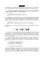
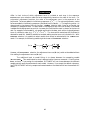
capabilities. The name DISTANCE was chosen because it can analyze several forms of distance
sampling data (pg:4-7): line transect, point transect (variable circular plot) and cue-count. By
contrast, TRANSECT was designed only for line transect data. In addition, the following features
have been added:
1. A wider choice of estimation models developed around a key/adjustment function (pg:46-48)
approach is included. Monotonicity constraints can be imposed on the models (pg:73). The "best"
model is selected from the chosen set of models (pg:73-77).
2. Several methods of adjustment term selection (pg:112,399-400) are available including sequential,
forward selection and fitting all possible combinations. In addition, specific adjustment terms can
be selected.
3. Clustered populations (i.e., animals observed in groups) (pg:12-13) are fully supported with sizebias analysis (pg:79-80) of expected cluster size and estimation of cluster density and
density/abundance of animals.
4. Stratified estimates of density and abundance can be constructed (pg:99-102).
5. Both left truncation (pg:15,273-277,377-379) and right truncation (pg:15,50,106-109) of the data
are supported .
6. Bootstrap re-sampling can be requested for robust estimates of variance (pg:94-96,119-120,155158).
DISTANCE understands and interprets a relatively simple command language. You "tell"
DISTANCE what you want to do by entering commands and data. The command approach was
chosen over a menu or question-answer interface because it easily allows the program to be used in
either interactive or batch mode (commands and data stored in files). This Guide describes the
commands and the way you will use them to analyze a set of data. In addition, we give several
examples showing the commands and data used as input and an explanation of the output.
INTRODUCTION
Installation Instructions
A single floppy disk accompanies this manual. It contains the following files that must be
installed before use:
DIST.ARC
README
INSTALL.BAT
EXAMPLES.ARC
PKUNZIP.EXE
- contains the executable program and help files
- installation instructions and other notes as needed
- batch file for program installation
- contains example input files
- program to unpack the .ARC files
We assume that you will be installing the software onto your hard disk which is designated
by C: and the installation floppy disk is in drive A:. If either disk is designated by another letter,
use that letter wherever we use C: or A:. Create a separate directory for the DISTANCE program
and associated files, by entering the following commands:
C:
CD\
MD YourDirectory
and replace YourDirectory with the name you want to give the directory (e.g., DISTANCE). After
creating a directory, install DISTANCE by entering the following:
A:INSTALL A: YourDirectory
For example,
A:INSTALL A: C:\DISTANCE
will install the software from drive A: into the directory DISTANCE on drive C:. Various files will be
installed:
1) DIST.EXE, the default executable file,
2) DISTL.EXE, an alternate executable file,
3) DIST.HLP, a text document containing help accessed by the program,
4) BROWSE.COM, a file listing utility,
5) README, a text file containing any corrections or new material not in this Guide, if needed, and
6) numerous template and example input files described in the EXAMPLES section.
2
INTRODUCTION
Program Requirements and Limitations
DISTANCE will only run on an IBM-PC or compatible microcomputer. A numeric coprocessor is not required but will improve the speed substantially (note: a co-processor is built into
an 80486DX processor or above). Approximately 1 MB of disk space plus additional space for input
and output files is required. Also, your computer's configuration file (CONFIG.SYS) should specify
FILES=20 or greater.
Available conventional memory should be sufficient on a machine with at least 640K of
memory unless numerous TSR (Terminate-Stay-Resident) programs or large device drivers (e.g.,
network drivers) are used. A problem exists, if either of the following error messages is given upon
running DISTANCE:
Not enough memory
or
Heap space limit exceeded.
Check the amount of free (available) memory for your computer with either of the DOS commands,
CHKDSK or MEM. Several solutions are given below for insufficient memory:
1) Load device drivers or TSR's into high memory, if you have DOS 5.0 or higher,
2) Use the alternate executable file (described below) which requires less memory but runs slower,
3) Reduce the memory setting for the overlay area (described below), or
4) Do not load optional TSR's or device drivers while running DISTANCE.
It is possible to change the memory requirements within certain limits. If you increase the
memory, the speed may increase and vice versa. The program memory is changed by setting the
environment variable BLINKER with the set command, before running DISTANCE. The format of
this command is SET BLINKER=/OOxx , where OO represents Overlay Opsize and xx is the amount
of memory in kilobytes (KB). The default value is 40 and it can be set to as low as 28 and as high
as 128. If you increase the memory requirements beyond the amount of free conventional memory,
a fatal error will be given when you attempt to run the program. An example setting is, SET
BLINKER=/OO28, which will decrease the memory requirements by 12K.
Two executable files are included to provide some flexibility in memory, speed and limits on the
amount of data that can be analyzed. The requirements and limits of each are as follows:
DIST.EXE - requires approximately 480K of conventional memory and has the following limits:
1000 observations, 700 samples, 100 strata.
DISTL.EXE - requires approximately 470K of conventional memory and has the following limits:
5000 observations, 2000 samples, 400 strata.
DISTL requires less memory and has larger limits only because the program is heavily overlaid and
as a result will run more slowly. Hopefully, the limits of DIST.EXE will be sufficient for most
applications. If so, you can save disk space by deleting DISTL.EXE after it is installed. If you choose
to use DISTL.EXE, do either of the following:
1. use the command DISTL in place of DIST to execute the program, or
2. rename DIST.EXE to another filename and rename DISTL.EXE to DIST.EXE.
3
OVERVIEW
OVERVIEW
How to Start DISTANCE
If you want to start DISTANCE from any disk drive and directory, place YourDirectory
in the computer's PATH statement (e.g. SET PATH=C:\;C:\DOS;C:\YourDirectory). Then simply
enter:
DIST
to start the program. If
entering:
YourDirectory is not included in your PATH, start DISTANCE by
YourDirectory\DIST
YourDirectory is the directory in which you installed DIST.EXE or change to
YourDirectory (CD \YourDirectory) prior to issuing the DIST command. Either of the above
commands runs DISTANCE interactively. DISTANCE displays a title screen and the DISTANCE>
where
prompt on the screen. DISTANCE is ready for you to enter commands and data from the keyboard.
Alternatively, DISTANCE can read commands and data entered into text files with an editor (e.g.,
EDIT) or saved from within DISTANCE (see the ASSIGN and STORE commands described later).
The latter approach, which eliminates redundant entry of commands and data, is described under
Batch Operation and the ASSIGN command. Until you become familiar with DISTANCE, we
recommend entering commands and data interactively.
A Simple Example
DISTANCE needs three types of information to perform an analysis:
1) OPTIONS - defines the type of sampling and data, measurement units, and various other settings
which affect data entry and analysis,
2) DATA - defines the sampling structure (strata & samples), sampling effort (e.g., line length), and
appropriate observation data (i.e., distance and cluster size), and
3) ESTIMATE - defines the parameters to be estimated, how the data are to be treated in the
analysis, which estimators are to be used, and how variances are to be estimated.
This information is entered via commands that define option values, structure data input, and
initiate and control estimation. Reasonable default values have been chosen for many of the options.
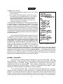
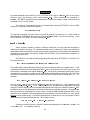
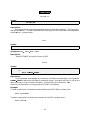
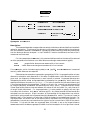
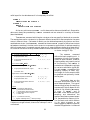
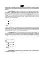
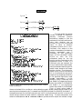
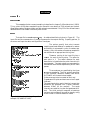
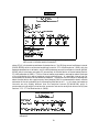
Figure 1 on the next page gives an example of command and data input, which are organized
into sections (procedures) corresponding to the type of information. For this example, the Options
section defines:
1) line transect sampling was used,
2) line length is measured in miles,
3) density is to be expressed in numbers per hectare, and
4) distance (perpendicular) is measured in intervals of 1 foot to a maximum distance (width)
of 4 feet.
4
OVERVIEW
The Data section defines:
1) 4 lines were sampled with lengths of 11.2, 14.3, 5.6 and
111.2 miles, and
2) the number of animals sighted in each of the 4 1-foot
intervals for each line (sample) (e.g., for line 2: 4 were
seen at distances between 0 and 1 foot, 3 were seen
at distances greater than 1 foot but within 2 feet,
likewise none were seen between 2 and 3 feet, and
2 were seen between 3 and 4 feet).
Two analyses are requested (one for each Estimate procedure).
In each analysis, 3 estimators are defined from which
DISTANCE chooses the "best" model (pg:73-77). In the second
analysis, the observations beyond 3 feet are truncated (pg:15).
Between the first and second analysis, the output is displayed
(List) to the screen for review. Notice that the options and data
are retained for the second analysis but estimate commands are
not retained (i.e., each ESTIMATOR command was repeated in
the second analysis).
Options;
Type=Line;
Length/Units='Miles';
Area/Units='Hectares';
Distance/Intervals=0,1,2,3,4
/Units='Feet';
End;
Data;
Sample/Effort=11.2;
5,6,2,1;
Sample/Effort=14.3;
4,3,0,2;
Sample/Effort=5.6;
2,0,1,0;
Sample/Effort=111.2;
15,6,7,0;
End;
Estimate;
Estimator/Key=Hazard;
Estimator/Key=Hnormal;
Estimator/Key=Uniform;
End;
List Output;
Estimate;
Estimator/Key=Hazard;
Estimator/Key=Hnormal;
Estimator/Key=Uniform;
Distance /Width=3;
End;
Not all input to DISTANCE will look exactly like Figure
1. However, it does illustrate the basic structure of input to
DISTANCE and the interactive nature of the analysis. Not all
of the possible options need to be specified if the default values
are acceptable. For example, the command TYPE=LINE; could
be deleted for this example, because it is the default value. The
format for data entry will vary depending on the type of
Figure 1. Example input file.
sampling and data defined by the options. In this example, the
Distance command within Options, defines grouped
(interval) distance data (pg:14) will be entered (i.e., the number of observations within each distance
interval is entered rather than the distance for each observation). We have created numerous
template files like Figure 1 that are installed into YourDirectory. The template files, which are
described in the EXAMPLES section, provide generic sets of commands and illustrate the data
format for various sampling situations. They can be modified with any text editor to include your
data and other commands or options for your specific analysis.
Entering Commands
The three primary commands issued at the DISTANCE> prompt are: 1) OPTIONS;, 2) DATA;,
and 3) ESTIMATE;. These commands initiate a procedure to begin entering a section of input and
change the prompt to OPTIONS>, DATA>, and ESTIMATE>, respectively. A section of input is
completed by entering the command END;. After completing the OPTIONS> and DATA> input
sections, the DISTANCE> prompt will reappear. However, after completing the ESTIMATE> section,
the analysis is performed before the DISTANCE> prompt reappears.
You can issue the OPTIONS, DATA, and ESTIMATE commands repeatedly and in any order;
however, the order is important in most circumstances. For example, data must be entered before
estimation is initiated and options which define the type of data, must be entered before entering
the data, unless the default values are acceptable. However, after entering data or performing an
analysis, options which do not change the basic data format can be changed. If you change options,
5
OVERVIEW
it is only necessary to set those options you want to change. All unchanged values remain as they
were last set. Unlike OPTIONS>, if you re-enter DATA>, previously entered data are cleared from
memory. The ESTIMATE> procedure can be re-entered any number of times without regard to
previous analyses.
Be aware of the command prompt because different commands are accepted at each prompt.
Some commands have the same name but perform different functions at different prompts. For
example, the DISTANCE command at the OPTIONS> prompt defines how the distance data will be
input, but at the ESTIMATE> prompt, the DISTANCE command defines how distances will be
analyzed. The header at the top of each page in this Guide identifies the appropriate prompt for
the command.
Except for the distance (or frequencies) and cluster size measurements, all information is
entered via commands. The format for entering data varies depending on the type of data and is
described in detail in the DATA> section.
The information contained in each command varies but the general syntax for a command
is the same for all commands. The general command syntax is:
command_base /switch1 /switch2 ... /switchn;
The command_base can be one of the following forms:
command_name
or
command_name=list
where list is one or more elements separated by commas. A switch can also be one of the
following forms:
switch_name
or
switch_name=list
where list is one or more elements separated by commas. Use commas to separate list elements,
not spaces. If the elements are separated by spaces, unpredictable results will occur. The switches
are not required but the base portion of the command is required. The base portion is either just the
command name or a command name followed by = and a list of one or more elements. For example,
for the ASSIGN OUTPUT command,
ASSIGN OUTPUT=FILENAME
is the base portion of the command.
Each command must end with a semi-colon ( ; ). A command can exceed more than one line
but cannot exceed 255 characters. Commands can only be split across lines between switches and
between list elements. Blank space is allowed within commands except embedded spaces are not
allowed within command and switch names and list values. All characters beyond the semi-colon
are ignored and can be used as comments. The following are some examples which demonstrate
valid and invalid ways of entering commands:
6
OVERVIEW
Valid command syntax
Invalid command syntax
ASSIGN INPUT = FILE.TST/NOECHO;
ASSIGN I NPUT=FILE.TST/NOECHO;
or
or
ASSIGN INPUT=FILE.TST
/NOECHO
;
ASSIGN INPUT=
FILE.TST;
When commands are entered interactively and the [Enter] key is pressed before completing
the command, DISTANCE will respond with
[waiting for input]
This mode continues until you exceed 255 characters or a semi-colon is entered to complete the
command.
Commands can be entered in any combination of upper and lower case letters because all
characters are changed to upper case. For Titles and Labels, put characters within single quotes to
maintain lower case or to use special characters (e.g., / or ;). For example, Title='Analysis of
survey 1/14'; will be a valid command which will set the title to Analysis of survey 1/14
with the upper and lower case maintained in the output. If you wish to include a single quote in the
label or title, use two contiguous single quotes to specify a single quote in the label. For example,
/LABEL='Fred''s sample' will become Fred's sample in the output.
Command, switch and value names can be abbreviated to the fewest number of characters
that avoids ambiguity (e.g., entering D when DISTANCE and DENSITY are potential commands
would be ambiguous, but DI or DE would not be ambiguous). If the value is ambiguous or
unrecognized an error is issued which lists the potential values. However, if you enter extraneous
characters that do not match a name, the name will not be recognized. For example, DIX will not
be interpreted as DISTANCE and will generate an error. The best strategy is to use as few
characters as needed to make the command simple to type but readable.
Descriptions of the commands are given below. The commands are organized alphabetically
within input prompt (DISTANCE>, OPTION>, DATA>, and ESTIMATE>). For each command, the
format and description of the command are given. Examples are often given to illustrate the
command, and where appropriate, synonyms for command and switch names are listed. Similar
command descriptions can be obtained interactively within DISTANCE via the HELP command.
Obtain help with a particular command by entering at the appropriate command prompt:
HELP command_name;
For example at the DISTANCE> prompt, entering HELP ASSIGN; will display information about the
ASSIGN command. One or more screens of information will be displayed which are similar to the
format of the command descriptions given in this documentation. The lines ('| |') around a list of
items indicates that one item from the list should be chosen.
7
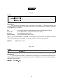
OVERVIEW
Program Files
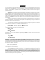
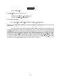
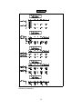
DISTANCE reads commands and data from input files and creates several output files as
illustrated below:
Input Files
>--DISTANCE-->
INPUT (keyboard)
DATA (keyboard)
Output
OUTPUT
RECORD
LOG
PLOT
BOOT
STATS
Files
(SCREEN & DIST.OUT)
(SCRATCH)
(SCREEN)
(SAS.PLT)
(BOOT.OUT)
(SCRATCH)
The default names for the input and output files are given in parentheses. (Note: SCRATCH is a
temporary file which disappears at the end of the program unless saved.) Each file can be given a
different name. The contents of each file and the ways in which they can be manipulated are
described below. The file manipulation commands are described under DISTANCE>. If DISTANCE
terminates abnormally, scratch files (e.g., beginning with XX or ZZ) that are normally deleted may
remain in your directory. You can delete these files, if they exist.
Input
INPUT and DATA are the 2 sources of input. INPUT is the primary source of commands and
data. DATA can be assigned to a separate file with the INFILE command. By default, command and
data entry are interactive (INPUT and DATA are assigned to the keyboard). Enter commands and
data interactively until you become familiar with DISTANCE. However, both input sources can be
independently assigned to disk files which contain the commands and data. For example, INPUT
can be assigned to a file DIST.INP with the ASSIGN command:
ASSIGN INPUT=DIST.INP;
which instructs DISTANCE to take all further commands and data from the file DIST.INP until it
encounters: 1) an EXIT;, 2) the end of the file, 3) a new ASSIGN command, or 4) an INFILE
command.
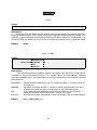
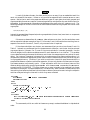
The DATA file contains the data to be entered at the DATA> prompt. By default, DATA is taken
from the INPUT file. Thus, if the INPUT file is assigned to a disk file, the DATA file is also assigned
to this same file by default. The DATA file can be assigned to its own separate file by using the
INFILE command (described under DATA> section). This can be done independently of assigning
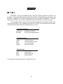
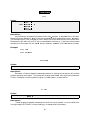
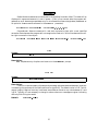
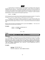
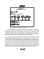
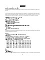
the INPUT file. Figure 2 gives an example to illustrate this relationship.
8
OVERVIEW
INPUT file assigned to DIST.INP:
INPUT file assigned to DIST.INP
DATA assigned to DIST.DAT
Enter:
ASSIGN INPUT=DIST.INP;
Enter:
ASSIGN INPUT=DIST.INP;
File: DIST.INP
File: DIST.INP
OPT;
DIST/INT=0,1,2,3;
END;
DATA;
SAMPLE /EFFORT=12.5;
10,8,6;
END;
ESTIMATE;
ESTIMATE/KEY=UNIF;
END;
OPT;
DIST/INT=0,1,2,3;
END;
DATA;
INFILE=DIST.DAT;
END;
ESTIMATE;
ESTIMATE/KEY=UNIF;
END;
File: DIST.DAT
SAMPLE /EFFORT=12.5;
10,8,6;
Figure 2. Example of INPUT and DATA file contents. The ASSIGN statement is entered
interactively to DISTANCE or the file is used as a batch input file (I=DIST.INP).
Output
The output files are:
OUTPUT
LOG
RECORD
PLOT
BOOTSTRAP
STATS
- analysis output
- error file
- record of all keyboard entry
- SAS or S+ command/data file for plots
- output of estimates from bootstrap runs
- estimation statistics file
All output files can be ASSIGNed and CLEARed. The first 3 can be LISTed and STOREd with the
appropriate commands (see DISTANCE> section).
LOG is used to record all errors and warning messages. Initially, LOG is the screen. If INPUT
and DATA are assigned to files, it is important to assign LOG to a permanent file so that error
messages are not missed amidst the stream of output. List this file to make sure that all
commands and data were entered properly. Error messages sent to the assigned log file are
no longer sent to the screen. If INPUT and DATA are assigned to files, their contents are echoed to
the log file, so an error message is associated with the incorrect entry. Set NOECHO on the INPUT and
DATA file assignment and the entries will not be echoed to the LOG file. The NOECHO is most useful
for lengthy DATA files after all errors have been eliminated.
9
OVERVIEW
RECORD is a complete recording of all keyboard entry. RECORD is initially a SCRATCH file
which is temporary and it is deleted upon exiting from DISTANCE. The RECORD file can be STOREd
or ASSIGNed to save its contents to repeat an analysis at a later time. Saving the RECORD is a useful
way to learn how to set up data files by entering commands and data interactively and having the
results stored in RECORD. All lines entered from the keyboard are sent to the RECORD including
incorrect commands. Edit the file to remove errors or unneeded commands before using as an
ASSIGNed INPUT file. RECORD can be LISTed to observe its contents and it can be CLEARed to
purge its contents.
OUTPUT contains the results of the data analysis. OUTPUT is sent to the screen and it is
appended to the default file named DIST.OUT. Suppress the file copy of the OUTPUT and only get
the screen copy by entering:
ASSIGN OUTPUT=SCREEN;
Suppress the screen copy and keep the file copy with the name "filename" by entering:
ASSIGN OUTPUT=filename/NOECHO;
OUTPUT can also be STOREd after it has been displayed on the screen. The STORE command copies
the output from the default file (DIST.OUT) to a file of your choice. When you STORE the OUTPUT
file, the default file (DIST.OUT) is CLEARed. New output is appended to the previous contents of
DIST.OUT by default. Use an ASSIGN, CLEAR or STORE command to avoid appending to
unwanted output. (Note: Do not use the DOS commands in this program to rename or delete a file
which is being used by DISTANCE) If you want to overwrite the default output file each time you
start DISTANCE, put the command ASSIGN OUTPUT=DIST.OUT/REPLACE; into the startup file
which is described below.
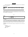
PLOT is created if the /SAS or /SPLUS switch is used with the goodness-of-fit (GOF)
command in the ESTIMATE> procedure. PLOT contains data and commands to create a high quality
graphics plot specifically with SAS/GRAPH or SPLUS. If you do not Assign a filename for PLOT, the
results are appended to the contents of the file SAS.PLT. PLOT can be used as input to other
graphics packages as well, if the SAS or S+ specific commands are removed. The data format is:
X (distance)
Histogram(x)
g(x) (or f(x))
Any graphics package which can produce 2 plots on the same graph can be used to plot the function
fitted to the data g(x) (or f(x)) overlaying a histogram representation of the data by connecting a line
to each point as a function of x. The values of Histogram(x) will plot horizontal bars and the values
of the function will produce a smooth curve. Note: for point transects, 2 figures are produced. The
first is the detection function, g(r), and the second is the probability density function of observed
radial distances, f(r).
STATS contains estimates and other statistics which are used internally by the program for
summarization and are not saved at program termination unless it is ASSIGNed to a disk file. For
each analysis (ESTIMATE), a set of records is output to STATS. The first record is the title of the
analysis. A blank record is output if you do not specify a title. The remaining records all have the
same format but some field meanings change depending on the record type, which is determined by
the value of Module and Statistic. The record structure is as follows:
10
OVERVIEW
Stratum
Sample
Estimator
Module
Statistic
Value
Cv
Lcl
Ucl
Df
- stratum number (or 0 if the estimate is for a sample or all data).
- sample number (or 0 if the estimate is for a stratum or all data).
- number of the estimator (in the order given in the Estimate procedure)
- number of the parameter module (Figure 3)
- number of the statistic within the parameter module (Figure 3)
- estimate value
- coefficient of variation of estimate or 0.0
- lower confidence limit or 0.0
- upper confidence limit or 0.0
- degrees of freedom for interval or 0
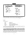
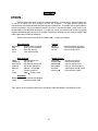
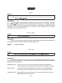
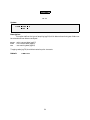
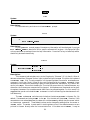
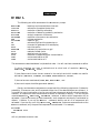
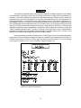
The modules and statistics within each module are listed in Figure 3 in the order in which they are
summarized in the output. The FORTRAN format for each record is:
(2(1x,i3),3(1x,i1),1x,g12.5,1x,f7.4,1x,2(g12.4,1x),i4).
Each field is separated by a space, so the records can be read into a spreadsheet or other program
as space delimited or as fixed-width format. The record for a module/statistic type is only output,
if it is relevant and it was computed in the analysis.
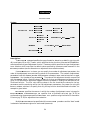
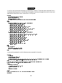
Module
Statistic/Parameter Estimate
1 - encounter rate
1 - number of observations (n)
2 - number of samples (k)
3 - effort (L or K or T)
4 - encounter rate (n/L or n/K or n/T) *
2 - detection probability
1 - total number of parameters (m)
2 - AIC value
3 - chi-square test probability (chi-p)
4 - f(0) or h(0) *
5 - probability of detection (Pw) *
6 - effective strip width (ESW) or
effective detection radius (EDR) *
3 - cluster size
1 - average cluster size *
2 - size-bias regression correlation (r)
3 - p-value for correlation significance (r-p)
4 - estimate of expected cluster size corrected for size-bias*
4 - density/abundance
1 - density of clusters (or animal density if non-clustered) *
2 - density of animals if clustered *
3 - number of animals if survey area specified *
(*) - implies a value for CV, LCL, UCL and DF are included, otherwise they are set to zero.
Figure 3. Definitions of module and statistic codes in STATS file.
11
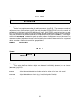
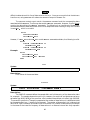
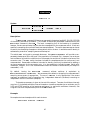
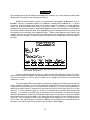
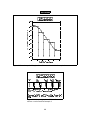
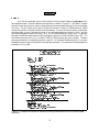
OVERVIEW
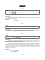
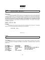
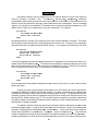
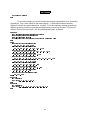
An example of the STATS file is given in Figure 4 for the example input file given in Figure
1. The first 4 records are the statistic records for the encounter rate module (the module field, the
fourth field from the left equals 1). For this module the estimator number is always 1 because these
statistics are independent of the estimator. The remaining records are all dependent on the
estimator and the estimator field is always 2 because the half-normal/cosine estimator was chosen
as the best estimator and it was listed second in the estimate procedure (Figure 1). Six records are
listed for each of the statistics in the detection probability module (field 4 = 2) and 1 record for the
density module (field 4 = 4). Records for cluster size are not listed because the input was for
unclustered data and the abundance statistic is not given because there was no area size specified.
Example input in Figure 1
0 0 1 1 1 54.000
.0000
0 0 1 1 2 4.0000
.0000
0 0 1 1 3 142.30
.0000
0 0 1 1 4 .37948
.4293
0 0 2 2 1 1.0000
.0000
0 0 2 2 2 130.11
.0000
0 0 2 2 3 .74194
.0000
0 0 2 2 4 .48112
.1137
0 0 2 2 5 .51962
.1137
0 0 2 2 6 2.0785
.1137
0 0 2 4 1 1.8610
.4441
.00000
.00000
.00000
.10253
.00000
.00000
.00000
.38332
.41399
1.6560
.48243
.00000
.00000
.00000
1.4046
.00000
.00000
.00000
.60388
.65219
2.6088
7.1791
0
0
0
3
0
0
0
53
53
53
3
Figure 4. Example STATS file for first estimate prcoedure of input file given in Figure 1
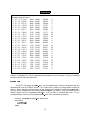
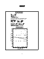
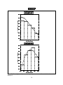
In addition, Figure 5 gives the resulting STATS file for the second estimate procedure in Figure 1
modified to show the results for each estimator (PICK=NONE). Records for the detection probability
and density modules are output in the STATS file for each estimator.
The BOOTSTRAP file contains a set of STAT records for each bootstrap. By default, a new
BOOTSTRAP file (BOOT.OUT) is created for each bootstrap analysis. If you want to append to the
results of other bootstrap results from the same analysis, ASSIGN the file with the /APPEND switch.
When the results of the bootstrap are summarized, all of the bootstrap estimates are included. This
enables you to run a large bootstrap analysis in batches (e.g., 5 batches of 200 to get 1000
bootstraps). If the bootstraps are appended, make sure you use the default SEED=0 which assigns
a random seed from the computer clock or change the SEED between batches; otherwise, the same
set of estimates will be repeated in each batch. The format of the records are as described under
STATS with the exception that a title record is not included.
12
OVERVIEW
Example input in Figure 1
0 0 1 1 1 51.000
.0000
0 0 1 1 2 4.0000
.0000
0 0 1 1 3 142.30
.0000
0 0 1 1 4 .35840
.4028
0 0 1 2 1 2.0000
.0000
0 0 1 2 2 108.33
.0000
0 0 1 2 4 .59869
.6316
0 0 1 2 5 .55677
.6316
0 0 1 2 6 1.6703
.6316
0 0 2 2 1 1.0000
.0000
0 0 2 2 2 106.91
.0000
0 0 2 2 3 .45113
.0000
0 0 2 2 4 .50318
.1354
0 0 2 2 5 .66245
.1354
0 0 2 2 6 1.9874
.1354
0 0 3 2 1 1.0000
.0000
0 0 3 2 2 106.69
.0000
0 0 3 2 3 .55245
.0000
0 0 3 2 4 .51245
.1208
0 0 3 2 5 .65047
.1208
0 0 3 2 6 1.9514
.1208
0 0 1 4 1 2.1871
.7491
0 0 2 4 1 1.8382
.4249
0 0 3 4 1 1.8721
.4205
.00000
.00000
.00000
.10437
.00000
.00000
.18694
.17385
.52156
.00000
.00000
.00000
.38386
.50536
1.5161
.00000
.00000
.00000
.40241
.51079
1.5324
.55459
.59323
.61075
.00000
.00000
.00000
1.2307
.00000
.00000
1.9173
1.0000
5.3493
.00000
.00000
.00000
.65959
.86837
2.6051
.00000
.00000
.00000
.65258
.82834
2.4850
8.6252
5.6960
5.7383
0
0
0
3
0
0
49
49
49
0
0
0
50
50
50
0
0
0
50
50
50
26
4
4
Figure 5. Example STATS file for second estimate prcoedure of input file given in Figure 1 modified
to output results from each estimator.
Startup File
An ASCII file named STARTUP.DST can be created which contains commands that are
executed each time DISTANCE starts. This is particularly useful to change default values for
options. As an example, assume that all of your sampling is from point transects (TYPE=POINT;)
and you want to squeeze all of the output (SQUEEZE=ON;), by default. Also, you would like the
default output file to be named DISTANCE.LST and you want it replaced each time. This is
accomplished by creating a file named STARTUP.DST with the following contents:
ASSIGN OUTPUT=DISTANCE.LST/REPLACE;
OPTIONS;
TYPE=POINT;
SQUEEZE=ON;
END;
13
OVERVIEW
Any valid command can be used in this file. DISTANCE will look for STARTUP.DST in the current
directory and in the directory which contains DIST.EXE. After processing any commands in
STARTUP, DISTANCE prompts for more commands (if in interactive mode) or reads commands from
the INPUT file (if in batch mode).
The name of the STARTUP file can be changed when starting DISTANCE from the DOS
prompt, by including an optional argument:
DIST S=startfile
The optional argument will work when running the program interactively or in batch mode as
described below. DISTANCE will look for the file named startfile in the current directory. If the
file is not found, DISTANCE will look for STARTUP.DST.
Batch Operation
Batch operation (mode) is simply an efficient method of running numerous analyses by
reducing the amount of typing. All command and data entry is identical in batch and interactive
mode. Batch mode is equivalent to running the program interactively and using ASSIGN statements
to specify the input, output and log files, except that DISTANCE is terminated upon completion of
processing the input file.
DISTANCE is run in batch mode by specifying filenames when DISTANCE is initiated. The
full specification is:
DIST I=infile O=outfile L=logfile S=startfile
The outfile, logfile, and startfile specifications are optional because each has a default value. If left
unspecified, the output will be appended to DIST.OUT, the log output will come to the screen and
the startfile is assumed to be named STARTUP.DST. We strongly recommend specifying a log file
and examining its contents to make sure all commands and data were entered correctly. All of the
switches for the ASSIGN command can be used with the file specifications (except with S=). For
example,
DIST I=DIST.INP O=DUCKS.OUT/REPLACE/NOECHO
will use DIST.INP as the input file and DUCKS.OUT as the output file. It will replace any file
currently named DUCKS.OUT. If the /REPLACE switch is not used and the specified file already
exists, DISTANCE displays an error message and appends the output to the default file, DIST.OUT.
By default, output is also displayed on the screen as the data are read and analyzed. Using /NOECHO
after the output file suppresses the screen output. Spaces are not allowed anywhere within a file
specification nor between it and its associated switches; however, there should be one or more spaces
between the file specifications. The following would be an invalid way to run the program in batch
mode because the space indicated by the ^ will create an error:
DIST I= DIST.INP O =DIST.OUT/NOECHO
^
^
One way to reduce typing is to specify the ASSIGN statements for the OUTPUT and LOG file
in the INPUT file. For example, entering:
14
OVERVIEW
DIST I=DIST.INP
where DIST.INP has as its first 2 lines
ASSIGN OUTPUT=DIST.OUT/REPLACE;
ASSIGN LOG=DIST.LOG/REPLACE;
is the same as entering:
DIST I=DIST.INP O=DIST.OUT/REPLACE L=DIST.LOG/REPLACE
However, if the input file contains ASSIGN commands the O= and
those values.
L= assignments will not override
If you wish, explore running the program in batch mode, by using one of the example input
files which have been included on the installation disk. The example files are installed into
YourDirectory during the installation process (see Installation Instructions). These files have been
constructed from the examples in Burnham et al. (1980) and Buckland et al. (1993). All of the
example input files have a .inp file extension. Some of the example filenames are Pgxx.inp where
xx refers to the page number in Burnham et al. (1980). Other filenames are EXn.inp where n refers
to one of the numbers of the Illustrative Examples in Burnham et al. (1980) or CHxxx.inp which
refers to the chapter and example number in Buckland et al. (1993).
15
DISTANCE>
DISTANCE>
DISTANCE> is the initial command prompt. When the commands, DATA;, ESTIMATE;, and
OPTIONS;, are issued at the DISTANCE> prompt, the prompt is changed to DATA>, ESTIMATE> and
OPTIONS>, respectively. The valid commands for each of the prompts are defined in individual
sections of this Guide. Each section is identified by the outlined title on the top of the page.
Also, at the DISTANCE> prompt, file manipulation commands can be issued to assign, clear,
list, print and store files. DOS commands from within DISTANCE can be issued from this prompt.
The following are valid commands at the DISTANCE> prompt:
Procedure Initiation
- enter distance sampling data
- estimation of density
- sets various program options
DATA
ESTIMATE
OPTIONS
File Manipulation
- assign filenames
- clear file contents
- list file contents to screen
- print options/data
- store file contents
ASSIGN
CLEAR
LIST
PRINT
STORE
Miscellaneous
DOS
- execute a DOS command
EXIT
- exit program
HELP
- display help files
PAUSE
- pause execution
The commands are described below in alphabetical order.
16
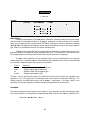
DISTANCE>
ASSIGN
Syntax:
|LOG
ASSIGN |PLOT
|RECORD
|BOOTSTRAP
|STATS
|
|/APPEND |
| = filename |
|
|
|/REPLACE|
|
|
;
or
ASSIGN
|/APPEND | |/ECHO |
OUTPUT = filename |
| |
| ;
|/REPLACE| |/NOECHO|
ASSIGN
INPUT
= filename /NOECHO
ASSIGN
HELP
= filename ;
or
;
or
Description:
Assigns filenames to the INPUT, LOG, RECORD, OUTPUT, PLOT, BOOTSTRAP, STATS
and HELP files. The filename must be a valid DOS filename or one of the following special names:
LOG can be SCRATCH or SCREEN, OUTPUT can be SCREEN, RECORD can be SCRATCH, and STATS
can be set to NULL to terminate output of statistics. If you use SCRATCH, the file is maintained (and
can be LISTed and CLEARed) but is deleted upon exiting DISTANCE unless it is explicitly stored
with a STORE command. Assigning HELP is only necessary if you change the name of the HELP file
or store it in a directory other than the one containing DIST.EXE. The default values for each file
are:
LOG
PLOT
RECORD
BOOTSTRAP
-
SCREEN
SAS.PLT
SCRATCH
BOOT.OUT
STATS
OUTPUT
INPUT
HELP
-
NULL
DIST.OUT
KEYBOARD
DIST.HLP
For output files, if you ASSIGN a file that already exists and do not specify either /APPEND
or /REPLACE, an error is issued and output is sent to the default file. For INPUT filenames, if the
file does not exist, an error message is issued. By default, the contents of INPUT files are echoed in
the LOG. Use the /NOECHO switch to override this default. If you use /ECHO (the default) for the
ASSIGN OUTPUT command, output is sent to the SCREEN as well as the file. If you use /NOECHO,
SCREEN output is suppressed. If sufficient memory is available, assigning the STATS or BOOTSTRAP
file to a RAMDRIVE, can reduce execution time.
Examples:
ASSIGN INPUT=TEST.INP;
ASSIGN OUTPUT=TEST.OUT/REPLACE;
ASSIGN PLOT=SPLUS.OUT/APPEND;
17
DISTANCE>
CLEAR
Syntax:
|LOG |
CLEAR |OUTPUT| ;
|RECORD|
Description:
CLEARempties the contents of the
file if the LOG file is the SCREEN.
Example:
LOG, OUTPUT or RECORD files. It has no effect on the LOG
CLEAR OUTPUT;
DATA
Syntax:
DATA ;
Description:
DATA initiates a separate command processor for entering distance data. The prompt will
change to DATA> . See the section on the DATA> prompt for further information.
DOS
Syntax:
DOS command_name ;
Description:
Executes the DOS command given by command_name and then returns back to the
DISTANCE> prompt. This will work for DOS commands and small programs. It is limited by the
amount of free memory available on your computer.
If a command_name is not given, the DOS prompt will appear. DISTANCE remains in the
background and you can issue several DOS commands. This is termed "shelling out". It is necessary
to type EXIT at the DOS prompt to return to DISTANCE. Do not issue the command to start
DISTANCE again because this will run DISTANCE within itself. Unexpected and possibly
unpleasant results will occur.
Examples:
DOS EDIT filename;
DOS DIR C:*.*;
18
DISTANCE>
ESTIMATE
Syntax:
ESTIMATE ;
Description:
ESTIMATEinitiates a separate command processor for estimation of density. The prompt will
change to ESTIMATE>. Various commands that can be given to control estimation are described in
the ESTIMATE> prompt section.
EXIT
Syntax:
EXIT ;
Synonyms:
STOP, QUIT, END, or BYE
Description:
Stops DISTANCE and returns control to DOS.
HELP
Syntax:
or
HELP;
HELP command_name;
Description:
If you type HELP; several pages of introductory information are displayed. If you type HELP
command_name; a description of the specific command is given. Use PgUp and PgDn or the up and
down arrow keys to scan the help information. Press the Esc key to leave help. HELP
should only be used when running program DISTANCE interactively.
Example:
To obtain a description of the SELECTION command at the OPTIONS> prompt, enter:
HELP SELECTION;
To obtain a description of the INFILE command at the DATA> prompt, enter:
HELP INFILE;
19
DISTANCE>
LIST
Syntax:
|LOG
|
LIST |OUTPUT | ;
|RECORD |
|DATA |
|OPTIONS|
Description:
LISTallows you to browse the contents of the LOG, OUTPUT or RECORD files. It will also
display the current data (LIST DATA) or the current values of the program options (LIST OPTIONS).
The command LIST is not intended for use in batch files. LIST sends output to the screen with
Browse and it will wait until an ESC key is pressed before continuing. If you want to output data
and options to the output file, use PRINT DATA; or PRINT OPTIONS; at the DISTANCE> prompt.
Example:
LIST LOG;
LIST OPTIONS;
OPTIONS
Syntax:
OPTIONS ;
Description:
OPTIONS initiates a separate command processor for setting various options which affect
program operation and output. The prompt will change to OPTIONS> after typing this command.
Further information on setting options is given in the OPTIONS> prompt section.
PAUSE
Syntax:
PAUSE ;
Description:
Pauses program in between commands until the Enter key is pressed. It can be useful when
running program DISTANCE in batch mode (e.g., for demonstration purposes).
20
DISTANCE>
PRINT
Syntax:
|OPTIONS|
PRINT |
| ;
|DATA |
Description:
Prints either the option values or the data values to the OUTPUT file but not to the screen.
STORE
Syntax:
|LOG |
|/APPEND |
STORE |OUTPUT| = filename |
|
|RECORD|
|/REPLACE|
;
Description:
The STORE command copies the contents of a program file into a named DOS file. If the file
specified by the filename already exists, an error is issued. Use /APPEND to append to an existing
file. Use /REPLACE to replace an existing file. If you specify a file which is currently being used
by the program, an error will be issued. The following example creates an error because ASSIGN
opens TEST.OUT and then STORE attempts to write to TEST.OUT which is already open:
ASSIGN OUTPUT=TEST.OUT;
STORE LOG=TEST.OUT;
Examples:
Store
LOG into the file TEST.LOG and append to the current contents of the file.
STORE LOG=TEST.LOG/APPEND;
Store OUTPUT into the file TEST.OUT and replace its contents if it already exists.
STORE OUTPUT=TEST.OUT/REPLACE;
21
OPTIONS>
OPTIONS>
Various options can be set to control program operation. Once an option value has been set,
it retains its value until you change it or exit the program. The data options define the
characteristics of the data collected and how they are to be entered. The model fitting options define
values to be used in fitting a probability density function to the distance data, some of which can
be overridden in the estimation procedure. Print options control the amount and format of program
output and bootstrap options control the number of bootstrap samples and the random number seed
used to generate a bootstrap sequence.
Below are the valid commands at the OPTIONS> prompt by category.
Miscellaneous
- options reset to default
- ends options command
- help with options
- lists option values
PRINT
SQUEEZE
TITLE
Data Options
- set area quantities
- set cue rate
- set distance quantities
- set length quantities
- SINGLE or CLUSTER
- sampling fraction
- POINT, LINE or CUE
EPSILON
ITERATIONS
LOOKAHEAD
MAXTERMS
PVALUE
SELECTION
Output
DEFAULT
END
HELP
LIST
- controls amount of output
- controls output pagination
- value of output title
Model Fitting
AREA
CUERATE
DISTANCE
LENGTH
OBJECT
SF
TYPE
- tolerance for fitting
- max # of iterations
- max for sequential fit
- max no. of adjustments
- significance level ("-level)
- term selection mode
Bootstrap
BOOTSTRAPS- no. of bootstrap samples
SEED
- random number seed
Each option and its possible values are individually described below in alphabetical order.
22
OPTIONS>
AREA
Syntax:
AREA
/CONVERT=value /UNITS='label' ;
Description:
This command defines the area unit for expressing density (D) (pg:1). The switches are:
/UNITS='label'
- a label for the unit of area of the density estimate. The single quotes are
only required to retain lowercase. Only the first 15 characters are used.
/CONVERT=value
-value specifies a conversion factor which is used as a multiplier to convert
the estimated density to new units for area. It is needed for atypical units.
If DISTANCE recognizes the measurement unit for DISTANCE (and LENGTH for line transects) and
if it recognizes the Area UNITS label, it will calculate the appropriate conversion factor. However,
if one or more of the UNITS is not recognized, you will need to specify the conversion value with the
CONVERT switch. The Area units recognized by the program are those listed under the DISTANCE
command and HECTARES (HEC) and ACRES (ACR). For example, the unit can be entered as
Squared Meters or Metres Squared because DISTANCE recognizes the unit based on the
character string MET. See the DISTANCE command below for a definition of recognized units
Default:
AREA /UNITS=HECTARES;
Examples:
Distances are measured in feet but analyzed in meters, length is measured in miles and
density is estimated as numbers per square kilometer. DISTANCE will do necessary unit
conversions because all unit labels are recognized.
DISTANCE/MEASURE=FEET/UNITS='Meters';
LENGTH/UNITS='Miles';
AREA /UNITS='Sq. kilometers';
BOOTSTRAPS
Syntax:
BOOTSTRAPS=value ;
Description:
'Value' is the number of bootstrap samples (pg:94-96, 119-120, 155-158) which should be
generated. For a reasonable variance estimate, this number should be at least 100. We recommend
setting BOOTSTRAPS=1000; to construct a bootstrap confidence interval.
Default:
BOOTSTRAPS=1000;
23
OPTIONS>
CUERATE
Syntax:
CUERATE = value1 /SE=value2 ;
Description:
For cue counting (pg:8-9, 270-275), 'value1' is the average rate at which animals issue visual
or auditory detection cues. The rate should be given in the same units of time as the values given
for sampling effort in the data. For example, if effort is measured in hours then the cue rate should
be number of cues per hour. The cue rate must be a positive number (>0). Optionally a standard
error for the cue rate can be given with 'value2'. This standard error is accounted for in the
estimated standard error of the density and abundance estimates. This option is only used if
TYPE=CUE is specified.
Default:
CUERATE=1/SE=0;
Example:
An estimate of the cue rate is 12 per hour with a standard error of 2 per hour. The sample
effort for this cue counting example be specified in hours sampled.
CUERATE=12 /SE=2 ;
DEFAULT
Syntax:
DEFAULT ;
Description:
This command resets all of the options to their default values. Remember that an option
remains in effect until it is changed or DISTANCE is terminated. The default values for each of the
options are:
PVALUE=0.15
SELECT=SEQUENTIAL
MAXTERMS=5
ITERATIONS=100
LOOKAHEAD=1
EPSILON=1.0E-7
PRINT=SELECT
SQUEEZE=OFF
BOOTSTRAPS=1000
SEED=0
SF=1
CUERATE=1/SE=0
24
TYPE=LINE
OBJECT=SINGLE
DISTANCE=PERP/EXACT/UNITS=METERS
LENGTH/UNITS=KILOMETERS
AREA/UNITS=HECTARES
OPTIONS>
DISTANCE
Syntax:
/WIDTH=width
/NCLASS=nclass
|PERP |
DISTANCE = |
| /CONVERT=value /UNITS='label'
|RADIAL|
/MEASURE='label' /RTRUNCATE=t
/LEFT=left
Synonyms:
;
| /INTERVALS=c0,c1,...,cu |
| /EXACT
|
RIGHT=WIDTH
Description:
This command describes numerous features about the distance data and defines the default
values for estimation. The format of the data entry within DATA> is determined by the values set
with this command. Whereas, the DISTANCE command at the ESTIMATE> prompt only determines
how the distance data are analyzed. In the EXAMPLES section the difference and use of the 2
commands are illustrated.
For line transect data (TYPE=LINE), this command defines whether the data will be entered
as either perpendicular distances or as radial distance and angle measurements (pg:4-6).
PERP
- perpendicular distance was measured for a line transect
RADIAL - radial distance and angle were measured in line transects
For TYPE=POINT (which includes trapping webs) or CUE (pg:6-8),
and only radial distances are expected.
DISTANCE=RADIAL is assumed
Distances can be entered as ungrouped or grouped (pg:13-14). Ungrouped implies an exact
distance is entered for each observation in the data. Grouped means a set of distance intervals is
given and the frequency of observations in each interval is entered. Ungrouped distances are
indicated by the switch /EXACT and grouped data is indicated by the /INTERVALS switch which also
specifies the distance intervals (c0-c1,c1-c2,c2-c3,...). The value c0 specifies the left-most distance and
cu the right-most distance for grouped data. Typically, c0=0 and cu=w. Intervals can also be specified
by using the /NCLASS and /WIDTH and optionally the /LEFT switch. These switches will create
'nclass' equal width distance intervals between the values of 'left' and 'width' (i.e., each interval is
of length (width-left)/nclass). For ungrouped data, it is also possible to specify left and right
truncation with the /LEFT and /WIDTH switches (pg:15). Any values outside of these bounds are
excluded from the analysis. Right truncation as a percentage of the observations can also be
specified for both grouped and ungrouped data with /RTRUNCATE switch. The value of t must be
between 0 and 1. In the analysis, no more than t*100% of the data is truncated from the right. For
ungrouped data, the width is set at the distance which represents the (1-t)*100% quantile. For
grouped data, intervals are truncated from the right as long as no more than t*100% of the data is
truncated. If t=0 and the data are ungrouped data, the width is set to the largest distance
measurement and if the data are grouped, the width is set to the endpoint for the right-most interval
25
OPTIONS>
with a non-zero frequency. For ungrouped data, if both the /WIDTH and /RTRUNCATE switch are
specified, the RTRUNCATE value specifies the value of width.
The DISTANCE command is also used to define the measurement unit for distances:
/MEASURE='label'
- a label for the units in which distance was measured. Single quotes are
only required to retain lowercase. Only the first 15 characters are used
/UNITS='label'
- a label for the units for distance after conversion, if any. Single quotes
are only required to retain lowercase. Only the first 15 characters are used.
/CONVERT=value
- value specifies a conversion factor which is used as a multiplier to convert
the input distances for atypical units.
MEASURE and UNITS switches are used to convert from the unit in which the data are recorded and
entered (MEASURE) to the unit for analysis (UNITS). It is not necessary to convert distances to
different units for analysis as long as it is a unit that is recognized by DISTANCE (see list below).
It is only provided as a convenience and it is probably easier to leave measurements in their original
units. If you do convert units, take note that values such as f(0), h(0), effective strip width (ESW)
(pg:23,56) and effective detection radius (EDR) (pg:154,175) are expressed in the converted units.
Thus, the point estimate and standard errors will change by the conversion factor from the measured
to analysis units. If you are not converting distance units, you can specify the units with either
switch (/MEASURE or /UNITS). The most common measurement units are recognized by DISTANCE
and there is no need to enter a conversion value (/CONVERT= value). The following are the
recognized measurement unit labels:
CENTIMETERS
INCHES
METERS
FEET
KILOMETERS
YARDS
MILES
NAUTICAL MILES
Each label is recognized by its first 3 characters which allows variations in spelling. For example,
if you enter METRES, it will use METRES as the label and will recognize it based on MET. Values
are given in uppercase but can be entered in upper or lowercase. If DISTANCE recognizes the
/UNITS and /MEASURE labels and you specify the /CONVERT= switch it will display a warning
message that you are overriding the conversion value. Values for /WIDTH, /LEFT, and
/INTERVALS should be given in original measurement units and not in converted units.
Default:
DIST=PERP/UNITS='Meters'/MEASURE='Meters'/EXACT/LEFT=0/RTRUNCATE=0;
Examples:
Perpendicular distance measured in intervals of 2 feet to a distance of 10 feet and converted
to metres (meters) for analysis. The grouped data are entered as the frequency of observations in
each of the 5 distance intervals (see DATA>). Notice that WIDTH is specified in the original
measurement units of feet and not in meters.
DIST=PERP /MEASURE='Feet' /UNITS='Metres' /WIDTH=10 /NCLASS=5 ;
26
OPTIONS>
Radial distance measured and analyzed in the specified intervals of feet. The label will be
displayed in uppercase because it is not in quotes. If this is line transect data the program will
generate an error because grouped data entry is not allowed for distance/angle data (see SMEAR as
an option for the DISTANCE command in the ESTIMATE procedure).
DIST=RADIAL /MEASURE=Feet /INTERVALS=0,2,5,8,12,25;
Perpendicular distance measured in rods and converted to feet with a user specified
conversion factor because the program will not recognize the Rods unit. 10% of the observations will
be right truncated in the analysis.
DIST=PERP /MEASURE='Rods' /UNITS='Feet' /CONVERT=16.5 /RTRUNCATE=0.10;
END
Syntax:
END ;
Description:
END completes entry of options and returns to the Distance> prompt.
EPSILON
Syntax:
EPSILON=value ;
Description:
'Value' is a relative measure of closeness of parameter estimates obtained between iterations
in assessing the maximum of the likelihood function (pg:65-66). The default value is 1.0E-7 which
means roughly 6 digits of accuracy is achieved. EPSILON can be set to any value between 0.1 and
1.0E-8. Typically, it is not necessary to change its value unless error messages are given indicating
difficulty with fitting the model.
Default:
EPSILON=1.0E-7;
27
OPTIONS>
HELP
Syntax:
HELP;
or
HELP command_name;
Description:
If you type
HELP; several pages of introductory information will be displayed. If you type
HELP command_name; a description of the specific command will be given. Use PgUp and PgDn
or the up and down arrow keys to scan the help information. Press the 'Esc' (Escape) key to leave
help. HELP should only be used interactively. It will work in batch mode, but it will interrupt
processing until you press the 'Esc' key.
ITERATIONS
Syntax:
ITERATIONS=value ;
Description:
'Value' is the maximum number of iterations that the algorithm will perform to determine
the parameters that maximize the likelihood function (pg:65-66).
ITERATIONS=100;
Default:
LENGTH
Syntax:
LENGTH /CONVERT=value /UNITS='label' /MEASURE='label' ;
Description:
This command sets the measurement unit for line length (pg:4-6) and any desired conversion
to different units for analysis. It is not necessary to convert line length, but may be desirable
depending on the original units.
/MEASURE='label' - a label for the units in which line length was measured. Single quotes
are only required to retain lowercase. Only the first 15 characters are used.
/UNITS='label'
- a label for the units for length after conversion, if any. Single quotes are
only required to retain lowercase. Only the first 15 characters are used.
/CONVERT=value - value specifies a conversion factor which is used as a multiplier to convert
length measured in atypical units.
28
OPTIONS>
See further explanation under DISTANCE for the /MEASURE,
LENGTH command is used for line transects only.
/UNITS and /CONVERT switches. The
Default:
LENGTH /UNITS=KILOMETERS /MEASURE=KILOMETERS;
Example:
Length is entered in miles but converted to kilometers for display and analysis.
LENGTH /UNITS='Kilometers' /MEASURE='Miles' ;
LIST
Syntax:
LIST;
Description:
Lists current values of the program options and the program limits to the screen.
LOOKAHEAD
Syntax:
LOOKAHEAD=value ;
Description:
For term selection modes SEQUENTIAL and FORWARD (see SELECTION), 'value' specifies
the number of adjustment terms which should be added to improve the fit, before the added terms
are considered to be non-significant (pg:399-400). For example, if LOOKAHEAD=2 and a model with
2 adjustment terms does not significantly improve the fit over a model with 1 term, a model with 3
adjustment terms is fitted. If the 3-term model is an improvement over a 1-term model, the
algorithm will continue with the 3-term model as the new base model. If it is not an improvement,
the 1-term model would be chosen. If LOOKAHEAD=1 (the default), in the above example, the 3-term
model would not have been examined because upon finding the 2-term model was not an
improvement, the 1-term model would have been used.
Default:
LOOKAHEAD=1;
29
OPTIONS>
MAXTERMS
Syntax:
MAXTERMS=value ;
Description:
'Value' is the maximum number of model parameters (pg:62-68). The maximum number of
adjustment terms (defined as m, pg:65) that may be added is MAXTERMS minus the number of
parameters in the chosen key function (defined as k, pg:65). MAXTERMS must be less than or equal
to 5. This option is only useful to limit the number of model combinations with the term selection
mode that considers also possible combinations of adjustment terms (SELECTION=ALL). Use the NAP
switch on the Estimator command to specify an exact number of adjustment terms to be used. The
maximum number of adjustment terms is also limited by the number of observations for ungrouped
data or number of distance intervals for grouped data.
Default:
MAXTERMS=5;
OBJECT
Syntax:
|SINGLE |
OBJECT=|
| ;
|CLUSTER |
Description:
This option defines whether objects are detected individually (SINGLE) or as clusters
(CLUSTER) (pg:11-13).
SINGLE
- Object always detected as a single animal or other entity (e.g., duck nest)
CLUSTER
- Object detected as a cluster (e.g., herd, flock,pod of whales)
Default:
OBJECT=SINGLE;
30
OPTIONS>
PRINT
Syntax:
|SELECTION|
PRINT=|RESULTS | ;
|ALL
|
|SUMMARY |
Description:
This option sets the default level of printing in the output. The various settings are
hierarchical and more control over the amount of results can be obtained with the PRINT command
in the ESTIMATE> procedure.
ALL
SELECTION
RESULTS
SUMMARY (NONE)
- print fitting iterations, model selection results and estimation results
- print model selection results and estimation results
- print estimation results only
- only summary tables are printed
Note: if you choose RESULTS or SUMMARY, warnings are not given about the algorithm having
difficulties fitting a particular model or constraining the fit to achieve monotonicity.
Default:
PRINT=SELECTION;
PVALUE
Syntax:
PVALUE=" ;
Description:
" is the significance level of likelihood ratio tests (pg:74-75) to determine significance of
adding adjustment terms and is the default value for the significance test for size-bias regression
of cluster sizes (pg:79-80)
Default:
PVALUE=0.15;
31
OPTIONS>
SEED
Syntax:
SEED=value ;
Description:
SEED specifies the random number seed for generating a sequence of random numbers for
bootstrap samples (pg:155-158). 'Value' should be a large odd number preferably greater than
2,000,000. If you use the same seed, the same sequence of random numbers will be generated. You
can use SEED=0; (the default) which will use a value from the computer's clock to generate a seed.
Default:
SEED=0;
SELECTION
Syntax:
|SEQUENTIAL|
SELECTION= |FORWARD | ;
|ALL
|
|SPECIFY |
Description:
This command specifies the default mode for adjustment term selection in the ESTIMATE
procedure for fitting the detection function. The /SELECT switch of the ESTIMATOR command
overrides the default value. See the ESTIMATE> section for a description of adjustment term and
model selection.
SEQUENTIAL - add adjustments sequentially (e.g., for simple polynomial, in increasing order of
SPECIFY
the exponent).
- equivalent to forward selection in regression; select the adjustment term which
produces the largest increase in the maximum of the likelihood function
- fit all combinations of adjustment terms with the key function and use the
model with smallest Akaike Information Criterion (AIC) value.
- user-specified number of adjustment terms and possibly order of the adjustments.
Default:
SELECTION=SEQUENTIAL;
FORWARD
ALL
32
OPTIONS>
SF
Syntax:
SF=c ;
Description:
SFdefines the value of the sampling fraction which is typically 1 (pg:53). However, if only one
side of a transect line is observed c=0.5, or if some fraction of the circle surrounding a point transect
is searched, c is the fraction searched (e.g.,c=0.5 if a semi-circle is observed). For cue counting, c
is the proportion of a full circle that is covered by the observation sector. For a sector of 90o (45o
either side of the line) with cue counting, c = 0.25
SF=1;
Default:
SQUEEZE
Syntax:
|ON |
SQUEEZE = | |
|OFF|
Synonyms:
;
ON=YES=TRUE, OFF=NO=FALSE
Description:
If this option is set 'off' a formfeed and title line is printed at the top of each page. If it is set
'on' , a formfeed is not included which has the effect of squeezing the output.
Default:
SQUEEZE=OFF;
TITLE
Syntax:
TITLE='yourtitle' ;
Description:
This command sets a value for the title which is printed at the top of each page. Yourtitle
should contain no more than 50 characters. Excess characters are not used. There is only 1 title
line. Re-specifying the title will replace the previous value.
33
OPTIONS>
TYPE
Syntax:
|POINT|
TYPE = |LINE | ;
|CUE |
Description:
This option defines the type of sampling (pg:3-8) which determines what types of data can
be entered and how data are analyzed.
POINT - point transect data (pg:6-7)
LINE - line transect data (pg:4-6)
CUE - cue counting data (pg:8-9)
Trapping webs (pg:7-8) should be treated as point transects.
Default:
TYPE=LINE;
34
DATA>
DATA>
Distance data are entered at the DATA> prompt. There are two ways of entering data: 1)
from the INPUT file (either the keyboard or an ASSIGN INPUT file), or 2) from a separate file
specified with the INFILE command.
Data are structured and entered in a hierarchical manner. The levels of the hierarchy can
be viewed as follows:
STRATUM
T
+))))))))))))2))))))))))))))),
*
R
SAMPLE 1
.......
SAMPLE k
T
T
+)))0))2))0))),
+)))0)))2))0)),
R R
R R
R R
R R
OBSERVATIONS FOR
OBSERVATIONS FOR
SAMPLE 1
SAMPLE k
The structure is specified by the order in which the commands and data are entered. A
STRATUM command is entered to begin a stratum and a SAMPLE command is entered to define and
begin a sample. All observation data (e.g., distances, cluster sizes) for a sample (i.e., line or point)
follow the SAMPLE command. For example, if the data are from two strata each with two samples,
conceptually the data are entered as follows:
STRATUM 1
SAMPLE 1
OBSERVATIONS
SAMPLE 2
OBSERVATIONS
STRATUM 2
SAMPLE 3
OBSERVATIONS
SAMPLE 4
OBSERVATIONS
FOR SAMPLE 1
FOR SAMPLE 2
FOR SAMPLE 3
FOR SAMPLE 4
It is not necessary to stratify the data. An equally valid layout for the above example would be:
SAMPLE 1
OBSERVATIONS
SAMPLE 2
OBSERVATIONS
SAMPLE 3
OBSERVATIONS
SAMPLE 4
OBSERVATIONS
FOR SAMPLE 1
FOR SAMPLE 2
FOR SAMPLE 3
FOR SAMPLE 4
Incomplete assignment of the data to strata is not allowed. The following example would not be a
35
DATA>
valid layout for the data because it is incompletely stratified:
SAMPLE 1
OBSERVATIONS FOR SAMPLE 1
STRATUM 1
SAMPLE 2
OBSERVATIONS FOR SAMPLE 2
At the very minimum one SAMPLE and its observation data must be defined. Observation
data must always be preceded by a SAMPLE command and are entered in a variety of formats
(described below).
The STRATUM command which begins a stratum, also may specify a label and an area size.
The most obvious use for a stratum is to represent different areas which were sampled or the same
area at different times. Estimates of density can be obtained separately by stratum and then
combined over strata. Use the DENSITY command at the ESTIMATE> prompt to define how stratum
estimates are combined. Another use for strata is to represent a second level of replicate sampling
within the same area. For example, several observers or several different platforms of observation.
Or strata can be used to stratify the data based on some characteristic of the population (e.g., sex,
or cluster size (pg:77-78)).
Point transects or cue counts (TYPE=POINT or =CUE):
1. Grouped radial distances
n1 , n2 , n3 ,..., nu ;
Ungrouped cluster sizes
s1 , s2 , s3 ,..., sn ;
2.
Ungrouped radial distances and
cluster sizes
r1 , s1 , r2 , s2 ,..., rn , sn ;
Line Transects (TYPE=LINE):
Radial distance & angle (DISTANCE=RADIAL)
3.
Ungrouped radial distances, angles,
r1 ,21 ,s1 ,...,rn ,2n ,sn ;
and cluster sizes
Perpendicular Distance (DISTANCE=PERP)
4.
Grouped perpendicular distances
Ungrouped cluster sizes
n1 , n2 , n3 ,..., nu ;
s1 , s2 , s3 ,..., sn ;
5.
Ungrouped perpendicular distances
and cluster sizes
x1 , s1 , x2 , s2 ,..., xn , sn ;
Legend:
For i=1,...,n (number of observations):
ri - ith radial distance measurement
xi - ith perpendicular distance measurement
2i - ith angle measurement in degrees
si - ith cluster size
For j=1,...,u (number of intervals):
nj - number of observations in jth distance interval
Table 1. Data entry formats assuming objects are clusters.
If objects are single animals, cluster size is always 1 and is
not entered.
36
The SAMPLE command
defines the basic sampling unit. It
represents a line for line transects,
a point for point transects, a web for
trapping webs, and a search period
for cue counting. Each SAMPLE is
treated as an independent replicate
for variance estimation (pg:90-98).
For each SAMPLE, a measure of the
sampling intensity or effort (e.g.,
line length for line transects) must
be specified and optionally a label
can be given.
Observation data are the
distances and cluster sizes for the
set of detected objects. The type of
data and their format (the way they
are entered) (Table 1) depend on the
values of the following OPTIONS:
1) TYPE, 2) OBJECT, and 3)
DISTANCE. TYPE defines the type of
sampling and determines the
appropriate distance measurement
(i.e., perpendicular distance (x) for
line transects and radial distance
(r) for point transects or cue
counting (pg:4-8)). OBJECT specifies
whether the population is clustered
DATA>
or not (pg:12-13). If the population is clustered, the size (s) of each observed cluster must be entered.
DISTANCE defines whether the distance data are entered as grouped (pg:14-15) or ungrouped (pg:13-
14) and whether distance for line transects is entered as perpendicular distance (x) or as a radial
distance (r) and angle (2) measurement from which perpendicular distance is calculated (i.e., x = r
sin(2)) (pg:4-6). For ungrouped distances, a measurement (e.g.,xi) is entered for each observed object
i. For grouped distances, the frequency of observations (n1, n 2, n3,...,n u) in each of u intervals are
entered (pg:14-15). The corresponding intervals of distance are defined by the set of cutpoints (c1,
c2, c3,...,cu) specified by the INTERVALS switch of the DISTANCE command.
Very few restrictions are applied to the data values. Distances (x or r) must be non-negative
($0). The distance units are defined by the DISTANCE command at the OPTIONS> prompt. Cluster
sizes (s) must be positive and the units are assumed to be integral values of animals, but the input
value is not restricted to be an integer. Angle (2) measurements (pg:5) should be entered in degrees
between 0-360o assuming the standard full circle representation. This representation for the angle
is provided as a convenience and it is not required. The orientation of the object is not included in
the analysis. Angle measurements are used only to calculate the perpendicular distance. At present,
angle measurements cannot be entered or used with point transects to indicate the orientation of
the object relative to the observer. Angle values can be limited to the half-circle interval (0-180o), or
to the quadrant (0-90o) by entering the acute angle formed by the line and the ray from the observer
to the object. At present, the angle and radial distance measurements cannot be entered as interval
(grouped) values. However, if the angle-distance data are collected in intervals, the analysis can be
modified with the SMEAR switch of the DISTANCE command at the ESTIMATE> prompt.
Frequencies (ni) for the grouped distance data must be non-negative. They are typically
integral values but are not restricted to integers. For grouped distance data with a clustered
population, DISTANCE checks to make sure that the sum of the frequencies of the grouped distances
matches the number of entered clustered sizes (i.e., n1+n2+þ+nu = n) An error message is issued
and the data are discarded, if they do not match. When the data are entered as frequencies, it is not
necessary to enter all of the frequencies in the tail, if they are zero. For example, if there were 7
distance intervals, the following could be entered: 5,2,0,1; and the remaining 3 frequencies for
intervals in the tail would be assumed to be zero.
The format for data entry depends on the data being entered. Table 1 displays the possible
formats assuming OBJECT=CLUSTER. If you enter the data from the keyboard, DISTANCE will
display the appropriate order and format. The same format should be used for data stored in a file
(INFILE). If there is any confusion as to the appropriate format, enter part or all of your data from
the keyboard to see how they should be formatted. Your keyboard entry can be stored in a file using
STORE RECORD from which a more complete input file can be constructed with an editor. Examples
of each of the data entry formats are given in template files described in the EXAMPLES section.
It is important that the data match the OPTIONS used to define the data. With very few
restrictions placed on the input data, it is possible to create situations in which data are input
without error but the data are incorrectly interpreted. Consider what would happen if the
population is treated as unclustered (OBJECT=SINGLE) but cluster sizes are entered with the
distances (format 2 or 5 in Table 1). DISTANCE would incorrectly treat each of the cluster sizes as
a distance and the result would be to double the sample size. Depending on the distance
measurement units, a plausible but incorrect detection curve may result. A similar situation could
occur if distance for line transects was defined as perpendicular (DISTANCE=PERP) but radial
distances and angles were entered.
37
DATA>
In each of the data formats, the data can be put on as many lines as needed but each line
must not exceed 80 characters. Values on a line must be separated with commas or one or more
spaces. Notice that a semi-colon separates different types of input data when both grouped and
ungrouped data formats are used for clustered populations and specifies the end of data input for
the sample. Unlike commands, information entered beyond the semi-colon will create an error. The
following example for format 1 would not be valid because distances are grouped and cluster sizes
ungrouped:
n1,n2,n3; s1,s2,s3,...,sn;
Instead, the grouped data (frequencies) and ungrouped data (cluster sizes) must start on a separate
line as shown in Table 1.
If there are no observations for a SAMPLE, data values are not given, but the semicolons must
still be entered to indicate a sample of size 0. For formats 1 and 4, two semicolons must be given on
separate lines and for formats 2, 3 and 5, only one semi-colon is required.
If the observed objects are clusters, we recommend that you do not use format 1 and 4 in
Table 1. Instead, we recommend that the measurements (distance and cluster size) be entered
ungrouped (EXACT) (formats 2 or 5), even if they were recorded in intervals (grouped). Use the
interval midpoint as the distance measurement for each observation in an interval. This enables
a more detailed analysis because the distance and cluster size measurements are paired for each
object. For instance, if a WIDTH is chosen which truncates some of the distance observations, it is
not possible to discard the appropriate cluster sizes unless the measurements are paired as they are
in ungrouped data entry. Likewise, if you wish to use cluster sizes which were observed within a
pre-specified distance or perform a size-bias regression, this can only be done if distances and cluster
size measurements are entered in pairs. Proper estimation with the true interval nature of the
distance data is obtained by specifying INTERVALS with the DISTANCE command at the ESTIMATE
prompt (pg:110-111,149-150). This also allows one or more intervals to be combined into larger
intervals in the analysis. A simple example with "unrealistically" small numbers of observations and
intervals is given below to show how interval distance data are entered as exact using the midpoint
and then analyzed using the intervals in which they were collected:
OPTIONS;
DIST=PERP;
<-- exact is assumed
OBJECT=CLUSTER;
END;
DATA;
SAMPLE/EFFORT=14.5;
.5 2 .5 4 .5 1 1.5 6 1.5 2 2.5 7;
SAMPLE/EFFORT=4.5;
.5 1 1.5 4 2.5 2 2.5 6;
END;
ESTIMATE;
DIST/INTERVALS=0,1,2,3; <-- data originally collected in these intervals
ESTIMATE/KEY=HN /ADJUST=POLY;
END;
The commands, which are valid at the
order.
DATA> prompt, are described below in alphabetical
38
DATA>
END
Syntax:
END ;
Description:
Finishes data entry and returns to the Distance> prompt.
HELP
Syntax:
or
HELP;
HELP command_name;
Description:
If you type HELP; several pages of introductory information will be displayed. If you type
HELP command_name; a description of the specific command will be given. Use PgUp and PgDn
or the up and down arrow keys to scan the help information. Press the Esc key to leave help. HELP
should only be used interactively.
INFILE
Syntax:
|/ECHO |
INFILE=filename |
| ;
|/NOECHO|
Description:
This command redirects data entry to the file given by "filename" (if it is found). After all
data are entered from "filename" further input is obtained from the INPUT file (either the keyboard
or ASSIGNed INPUT file). The only exception is if the specified data file contains another INFILE
command. It will then "chain" (jump) to the next file specified by the INFILE command. Upon
completion of the second file (assuming it does not have any INFILE statements), DISTANCE will
return to the INPUT file and not the data file. Thus the files cannot be truly "nested" because any
data after the first INFILE command will be ignored. Multiple INFILE commands can be given
throughout the INPUT file to enable several data files to be merged together. For this reason it is
suggested that you do not include the END; statement in the file containing the data because it will
halt data entry.
The ECHO and NOECHO switches control whether the data are ECHOed to the LOG file. By
default, if commands are being ECHOed to the LOG file, the data will be ECHOed; likewise, if the
commands are not echoed (NOECHO), the data will not be ECHOed by default (see the /ECHO switch
on the ASSIGN command). These default values can be changed by adding either the /ECHO or
/NOECHO switch. The /ECHO is most useful in tracking down errors in the data because errors are
printed in the LOG directly after the incorrect data line. If the data are not ECHOed, it may be
39
DATA>
difficult to determine which line of data contains the error. Once you are certain that the data are
free of errors, using /NOECHO will reduce the amount of output to the LOG file.
The INFILE contents must contain the SAMPLE command and the corresponding data
associated with the SAMPLE. The file may also contain STRATUM commands. However, the file cannot
contain the data without the SAMPLE commands. The following is an invalid use of the INFILE
command because the observation data for the first sample are either missing or they are included
in TEST.DAT, which is not valid:
DATA;
SAMPLE/EFFORT=1;
INFILE=TEST.DAT;
However, if
Example:
FILE1.DAT and FILE2.DAT contain SAMPLE commands and data, the following is valid:
DATA;
STRATUM /LABEL=STRATUM 1;
INFILE=FILE1.DAT;
STRATUM /LABEL=STRATUM 2;
INFILE=FILE2.DAT;
DATA;
INFILE=FILE1.DAT;
INFILE=FILE2.DAT /NOECHO;
END;
LIST
Syntax:
LIST;
Description:
Lists values of the entered data.
SAMPLE
Syntax:
SAMPLE /EFFORT=value
/LABEL='label name' ;
Description:
The SAMPLE command defines the sample effort and initiates entry of the observation data
for a sample. The sample-observation pairing is necessary for empirical and bootstrap variance
estimation (pg: 90-91, 94-96) of the encounter rate (numbers observed per unit effort) (pg: 186-198).
The encounter rate for the ith sample is computed as the number of observations (ni) detected divided
by the sample effort (e.g., li , length of a line transect). The number of observations (ni) is determined
after left or right truncation of the data (note: the notation for number of observations per sample
is the same as that used for frequency of observations in a distance interval but they represent
40
DATA>
different values). Sample 'effort' was chosen as a generic term to represent very different measures
of sampling intensity which determine the amount of area searched for the various types of distance
sampling.
For point transects, the basic unit of sample effort is 1 for each time a complete point or
web is sampled. If some constant fraction, c, of the complete circle is searched for all of the points,
it is easiest to set effort=1 and use the command SF=c at the OPTION> prompt, where c is the
proportion of the circle searched. However, if only some of the point transects are searched partially,
set the effort for those samples to the fraction of the circle searched. Do not set both the effort to c
and SF=c. As an example, if for 1 point transect only 1/2 the circle was searched once and the
remaining points were completely searched once, let SF remain at its default value of 1 and enter
the effort for each sample as follows:
DATA;
SAMPLE/EFFORT=0.5;
...
SAMPLE/EFFORT=1;
...
SAMPLE/EFFORT=1;
...
{etc}
If a series of point transects are surveyed along a line and the distance between the points is small
relative to the size of the area, it is more reasonable to consider the line of points as a replicate
rather than the point. In this case, each line would be represented as a sample and the effort would
be the number of point transects along the line (if c=1 for each point) or the sum of the fraction of
the circle observed at each point (if c < 1 for one or more points).
For line transect sampling, effort is the length of a line (li) for each time it is sampled. As
with point transects, if only 1 side of the line transect is searched, sampling effort can be adjusted
for a few lines by halving the line length or it can be adjusted for all lines by setting the value of
SF=0.5; at the OPTIONS> prompt to adjust all of the lines. A partial example is illustrated below,
with the first 3 lines each sampled a single time and the lengths are 10.5,12.1 and 1.5 miles
respectively.
OPTIONS:
LENGTH/UNITS='Miles';
END:
DATA;
SAMPLE/EFFORT=10.5;
...
SAMPLE/EFFORT=12.1;
...
SAMPLE/EFFORT=1.5;
...
{etc}
For cue counting, the sampling effort is the time spent searching. The discussion above
also applies to cue counting.
41
DATA>
In some studies, to increase the number of observations (of animals), lines or points are
sampled more than once in a short period of time (pg:91). These should not be treated as
independent spatial replicates. Instead, define a SAMPLE for each point or line but set effort to be
t*e, where t is the number of times a sample is searched and e is the effort for a single visit (e.g., e
is the length of the line or is 1 for a point transect (if c=1)). For example, if a point transect is
observed twice in a short time period, the sample is specified as:
SAMPLE /EFFORT=2;
All of the observations from both visits to the point would follow the SAMPLE command. Re-sampling
the same line or point for immobile objects is inappropriate for obvious reasons.
The /LABEL can be used to give a label for the sample which is used to label the output if the
density is estimated for each sample. The quote marks are only necessary to maintain lowercase
letters and to include the special characters "/" and ";". Only the first 50 characters of the label are
used.
Note: An early test version of DISTANCE used the syntax:
accepted, but the current syntax is preferred.
Examples:
SAMPLE=effort. That form is still
SAMPLE /EFFORT=1 /LABEL=SAMPLE A;
SAMPLE /EFFORT=14.2;
STRATUM
Syntax:
STRATUM
/LABEL='label name' /AREA=asize ;
Description:
The STRATUM command starts entry of the data associated with a stratum. The /LABEL
switch can be used to give a label that identifies the stratum in the output if density is estimated
separately for each stratum. The quote marks are only necessary to maintain lowercase letters.
Only the first 50 characters of the label are used. The /AREA switch specifies gives the size of the
stratum, if appropriate. The area size must be in the units specified by AREA/UNITS. For example,
if AREA/UNITS='Sq. Kilometers'; is given in OPTIONS>, STRATUM/AREA=1500; specifies an
area of 1500 square kilometers.
Examples:
STRATUM /LABEL=STRATUM A;
STRATUM;
STRATUM /AREA=1500 /LABEL='Plains area';
42
ESTIMATE>
ESTIMATE>
The following are valid commands at the ESTIMATE> prompt:
BOOTSTRAP
CLUSTER
DENSITY
DETECTION
DISTANCE
ENCOUNTER
END
ESTIMATOR
G0
GOF
HELP
MONOTONE
PICK
PRINT
SIZE
VARF
VARN
- bootstrap variance/confidence intervals
- estimation of expected cluster size
- resolution of density estimation
- resolution of detection probability estimation
- analysis treatment of distances
- resolution of encounter rate estimation
- initiates estimation
- model for g(x)
- estimate of g(0) and its standard error
- intervals for goodness-of-fit test/display
- help information
- monotonicity constraints on g(x)
- method of model choice
- detailed control of output
- resolution of expected cluster size estimation
- variance estimation of f(0)
- variance estimation of n
The commands are described below in alphabetical order. You will use these commands to define:
1) which quantities you want to estimate and at what level of resolution (DENSITY,
DETECTION, ENCOUNTER, SIZE ),
2) how distance and cluster size are treated in the analysis and which models are used for
estimation ( DISTANCE, CLUSTERS, ESTIMATOR, MONOTONE, PICK, GOF, G0),
3) how variances are estimated ( VARN, VARF, BOOTSTRAP), and
4) how much output should be generated ( PRINT ).
Density and abundance estimates are comprised of the following components: 1) detection
probability, 2) encounter rate, and 3) expected cluster size (if the detected objects are clusters). It
is possible to restrict estimation to one or more of these components without estimating density;
however, all components must be estimated to obtain an estimate of density. You will use the
commands DENSITY, DETECTION, ENCOUNTER, and SIZE to define which components will be
estimated. If you do not use any of these commands, each component and density is estimated, by
default. Likewise, if you use the DENSITY command, density and all of its components are
estimated. If you use any or all of the DETECTION, ENCOUNTER, and SIZE commands and not the
DENSITY command, only the specified components are estimated. For example,
ESTIMATE;
ENCOUNTER ALL;
END;
will only estimate encounter rate.
43
ESTIMATE>
Estimates of density and its components can be made at different levels of the sampling
hierarchy (Sample < Stratum < All). The DENSITY, DETECTION, ENCOUNTER, and SIZE
commands are used to specify the level at which each quantity is estimated. Different levels can be
used for the various quantities; although, some combinations are incompatible. An error message
is given, if the levels are incompatible. The lowest level of resolution specified for DENSITY is the
default level for each of its components, if they are unspecified. For example,
ESTIMATE;
ESTIMATOR/KEY=UNIFORM;
DENSITY BY STRATUM;
END;
will estimate density and each of its components for each stratum defined in the data. The lowest
level for density must coincide with a level assigned to encounter rate. The level of any component
cannot be lower then the lowest level specified for density. For example, the following is not valid:
ESTIMATE;
ESTIMATOR/KEY=UNIFORM;
DENSITY BY STRATUM;
DETECTION BY SAMPLE;
END;
If a size-bias regression estimate of expected cluster size is computed, the level for SIZE must be no
greater than the level for DETECTION. This feature is most useful for estimating density by stratum
when too few observations exist in each stratum to estimate f(0) (or h(0)). A solution is to assume
f(0) is the same for all strata, which is illustrated in the following example:
ESTIMATE;
ESTIMATOR/KEY=UNIFORM;
DENSITY BY STRATUM;
DETECTION ALL;
END;
All of the observations are pooled to estimate a common value for f(0), which is used in each stratum
density estimate.
Possibly the most confusing aspect of estimation with DISTANCE will be the specification
of models for detection probability and model selection. A model is specified with the ESTIMATOR
command which defines a type of key function and adjustment function. The adjustment function
is actually a series of terms which are added to the key function to adjust the fitted function to the
data (pg: 62-65). Model selection (pg: 73-77) includes 1) selecting how many and which adjustment
terms are included in the model (term selection) and 2) selecting a "best" model (estimator) from the
specified set of competing models.
The default method of selecting terms (term selection mode) is defined by the SELECTION
command under OPTIONS>. Its value can be overridden with the /SELECT switch of the ESTIMATOR
command. Related options include LOOKAHEAD and MAXTERMS. There are 4 types of term selection
modes described below: 1) SEQUENTIAL, 2) FORWARD, 3) ALL, and 4) SPECIFY. The maximum
number of adjustment terms that can be included in the model is limited by the value of ( MAXTERMS number of parameters in the key function) and less frequently by either the number of observations,
44
ESTIMATE>
for ungrouped data, or the number of distance intervals for grouped distance data. DISTANCE will
issue a warning message if the number of parameters is being limited by the amount of data.
Term selection mode SPECIFY implies the user will specify which adjustment terms are
included in the model. Typically, this is used to specify that a key function without adjustment
terms is to be fitted to the data, as in the following example:
ESTIMATE;
ESTIMATOR/KEY=HNOR/NAP=0/SELECT=SPECIFY;
END;
It is not necessary to include the /SELECT switch, but it will prevent DISTANCE from issuing a
warning message that you are specifying the model. It is also possible to specify any combination
of terms and give starting values for their coefficients. DISTANCE does not select the terms to
include in the model but does estimate the parameters to fit the model to the data. For example,
ESTIMATE;
ESTIMATOR/KEY=UNIFORM/NAP=2/SELECT=SPECIFY/ORDER=1,3;
END;
specifies the model as the following 2-term cosine series for which the parameters a1 and a2 are
estimated:
f(x)
' 1 1 % a1 cos Bx % a2 cos 3 Bx
w
w
w
.
ALL, as its name implies, examines all possible combinations of a limited number of
adjustment terms. If z is the maximum number of parameters (MAXTERMS=z) and k is the number
of parameters in the key function, then there are 2z-k combinations of the adjustment terms. Each
model is fitted to the data and the model with the smallest value of the Akaike's Information
Criterion (AIC) is selected.
SEQUENTIALand FORWARD both consider a subset of models with different combinations of
adjustment terms. For each of these term selection modes, a sequence of models is considered. An
adjustment term is added at each step of the sequence. The sequence of models can be represented
as:
M1 - key function with no adjustment terms
M2 - key function with 1 adjustment term
M3 - key function with 2 adjustment terms
.
.
Mv - key function with v-1 adjustment terms
A stopping rule (CRITERION) is either based on a likelihood ratio test or minimizing AIC. Model Mt
is chosen if there is no model in the sequence Mt+1,...,Mt+l which provides a significantly better fit as
determined by the specified CRITERION. The LOOKAHEAD option determines the length (l) of the
sequence of models that is examined before choosing model Mt. SEQUENTIAL and FORWARD only
45
ESTIMATE>
differ in their choice of which adjustment term is included at each step in the sequence.
SEQUENTIAL term selection adds the terms sequentially based on the order of the term. For
polynomial adjustment functions, the order of the adjustment term is the exponent of the
polynomial. Terms are added in the following sequence: (xt, xt+2,...). For cosine adjustments, cosine
terms are added in the following sequence: (cos(tBx/w),cos((t+1)Bx/w),...). The beginning value, t, is
determined by the shape of the key function. FORWARD selection adds 1 term at a time but not
necessarily in sequential order. For each model in the sequence, each term not already in the model
is added and the adjustment term which increases the likelihood the most is chosen as the term to
add. For example, to find model M2, z-k models are fitted to the data, each with a single adjustment
term of a different order (e.g., x2, x4, x6 , x8 ,or x10 ). The term which maximizes the likelihood is
selected for model M2. Model M3 would then consider adding another term not included in M2. With
FORWARD selection it is possible to select models that cannot be selected with the SEQUENTIAL
mode. For example, the following model might be chosen with FORWARD selection:
f(x)
' 1 1 % a1 cos Bx % a2 cos 3 Bx
w
w
w
.
However, with SEQUENTIAL selection, the adjustment term cos(3Bx/w), could not be added without
first adding the adjustment term cos(2Bx/w) .
The additional level to model fitting is to choose between the competing models
(ESTIMATORs). This model selection step is determined by the PICK command. It has 2 values:
NONE and AIC. If you assign the value NONE, DISTANCE will not choose between the different
models and will report the estimates for each model. However, if you accept the default value, AIC
(pg:75-76) DISTANCE will only compute estimates based on the model which has the smallest AIC
value.
46
ESTIMATE>
BOOTSTRAP
Syntax:
|/STRATUM |
BOOTSTRAP |
|
|/INSTRATUM|
/SAMPLES /OBS ;
Description:
The BOOTSTRAP command initiates a non-parametric bootstrap (pg:94-95, 119-120, 155-158)
of the density estimation procedure. The number of bootstraps performed is determined by the
BOOTSTRAP command in OPTIONS. The basic re-sampling unit of the bootstrap is a SAMPLE;
however, if strata are replicates they can also be re-sampled with the /STRATUM switch. If both are
specified, re-sampling occurs at both levels (see example below). The switch / INSTRATUM can be set
to restrict the re-sampling of samples or observations within stratum It would be used if density is
estimated by stratum or sampling was stratified apriori.
The switch /OBS can be set to re-sample distances. Using BOOTSTRAP/OBS; will provide a nonparametric bootstrap of f(0) or h(0) and, if the population is clustered, E(s). However, the variances
and confidence intervals are conditional on the sample size and do not include the variance of the
encounter rate. The /OBS switch has been included for completeness but its routine use is not
recommended. Reasonable confidence intervals for density could only be obtained by adding a
variance component for the encounter rate. It is also possible to include the /OBS switch with
/SAMPLES, however, this is not recommended unless the number of observations per sample is
reasonable ( > 15).
default, issuing the BOOTSTRAP command without switches is equivalent to
BOOTSTRAP/SAMPLES/INSTRATUM;. We recommend the default or dropping the /INSTRATUM if
sampling across strata is appropriate. The use of /STRATUM is only appropriate if the strata
By
represent an additional level of sampling (e.g., independent observers (stratum) traversing an
independent set of line transects (sample)).
The bootstrap summary is given at the end of the output. Two sets of confidence intervals
are given: 1) log-based confidence intervals based on a bootstrap standard error estimate, and 2)
2.5% and 97.5% quantiles of the bootstrap estimates (i.e., percentile confidence intervals). See
Program Files for a complete description of the BOOTSTRAP file.
Example:
Re-sample strata and samples within each stratum.
BOOTSTRAP /STRATUM /SAMPLES;
47
ESTIMATE>
CLUSTER
Syntax:
CLUSTER
/WIDTH=value
|/MEAN
|
|
|/BIAS=|
|
|
|
|
/TEST="
X
|
XLOG |
GX |
GXLOG|
|
|
|
|
|
;
Description:
The CLUSTER command, like the DISTANCE command, is used to modify the way the cluster
sizes are used in the estimate of density. By default, the WIDTH is chosen to match the truncation
value set by the DISTANCE command and DISTANCE computes a size-bias regression estimate
(/BIAS=GXLOG) by regressing the loge(s) (natural logarithm specified as log() in the output) against
ĝ(x), where x is the distance at which the cluster was observed.
The WIDTH switch specifies that only cluster sizes for observations within a distance less than
WIDTH are used in the calculation of the expected cluster size. This treatment of the data can only
be accomplished if the distances and cluster sizes are both entered as ungrouped.
The MEAN switch specifies that the expected cluster size is to be estimated as the average
(mean) cluster size. Likewise, the BIAS switch specifies that expected cluster size is to be estimated
by a size-bias regression defined by the value of the switch.
Value
X
XLOG
GX
GXLOG
Meaning
Regress cluster size against distance x
Regress loge(s) against distance x
Regress cluster size (s) against ĝ(x)
Regress loge(s) against ĝ(x)
The TEST switch specifies the value of the significance level to test whether the regression was
significant. If it is non-significant, the average cluster size is used in the estimate of density. The
default value for the significance level is set by PVALUE in OPTIONS. If the TEST switch is not
specified, the size-bias regression estimate will be used regardless of the test value.
Examples:
Estimate the expected cluster size from the loge (s) vs. ĝ(x) regression, but use the average cluster
size if the correlation is non-significant as determined by the "-level set with PVALUE (default=0.15).
CLUSTER /BIAS=GXLOG /TEST;
48
ESTIMATE>
DENSITY
Syntax:
|NONE
|
DENSITY by SAMPLE /DESIGN=|
| ;
|REPLICATE|
or
|NONE
|
DENSITY by STRATUM /DESIGN =|STRATA |
|REPLICATE|
|EFFORT|
/WEIGHT= |
|
|AREA |
|
|
|NONE |
or
;
DENSITY by ALL ;
Description:
These commands define the levels at which density estimates are made and how these
estimates are weighted. If the DENSITY by ALL; command is used or if none of the commands
(DENSITY, ENCOUNTER, DETECTION, SIZE ) are given, all of the data are used to make one
overall estimate of density.
If the DENSITY BY SAMPLE command is given, density is estimated for each sample. The
DESIGN value defines how the estimates should be treated to create a pooled estimate. If
DESIGN=REPLICATE (default), each sample is treated as an independent replicate from the stratum
or the entire area. In this case, the estimates are weighted by effort (e.g., line length) to get a
stratum density estimate (if DENSITY by STRATUM is also specified) or a pooled overall density
estimate (see eqns. 3.11-3.14 in Buckland et al. (1993)). If DESIGN=NONE, the sample estimates are
not pooled.
If DENSITY BY STRATUM is specified, an estimate is made for each stratum. A stratum
estimate is a pooled estimate of the sample estimates within the stratum, if DENSITY by SAMPLE;
is specified, or it is an estimate based on the data within the stratum. An overall (pooled) estimate
of density is made unless DESIGN=NONE is specified. If DESIGN=REPLICATE, the stratum estimates
are treated as replicates to create a pooled estimate and variance weighted by effort (eqns. 3.11-3.14
in Buckland et al. (1993), treating stratum as a sample). If DESIGN=STRATA, the pooled estimate
is a weighted sum of the estimates and the variance is a weighted sum of the stratum variances
(Section 3.8.1 in Buckland et al. (1993)). Weighting is defined by the WEIGHT switch. If
WEIGHT=NONE, the densities are summed, which is only useful if the population is stratified as by
sex or age. If WEIGHT=AREA, the densities are weighted by area (which is the same as adding
abundance estimates) and if WEIGHT=EFFORT, the densities are weighted by effort.
Prior to version 2.1, a combined estimate of abundance (N) was created by multiplying the
49
ESTIMATE>
combined density estimate by the sum of the areas specified on each of the STRATUM commands.
This produces obviously erroneous results when DENSITY by STRATUM/DESIGN=REPLICATE; is
used and the area size is repeated on each STRATUM. To avoid this problem in the following two
situations the combined abundance estimate uses the area from the first stratum:
1) DENSITY
by STRATUM/DESIGN=REPLICATE;
2) DENSITY
by STRATUM/DESIGN=STRATA/WEIGHT=NONE;
In all other cases, the area is totalled from all of the strata.
Default:
For DENSITY
For DENSITY
by SAMPLE: /DESIGN=REPLICATE
by STRATUM: /DESIGN=STRATA
/WEIGHT=AREA
Examples:
An estimate is needed for each stratum and it will be weighted by stratum area:
DENSITY BY STRATUM;
An estimate is needed for each stratum and there are enough observations in each sample to get an
estimate from each. The strata represent different platforms surveying the same area so the strata
are treated as replicates.
DENSITY BY SAMPLE;
DENSITY BY STRATUM /DESIGN=REPLICATE;
DETECTION
Syntax:
|SAMPLE |
DETECTION by |STRATUM|
|ALL
|
;
Description:
This command explicitly specifies that detection probability (and its functionals f(0), h(0))
should be estimated and the resolution at which the estimate(s) should be made (by SAMPLE, by
STRATUM, or ALL data).
Example:
Density is estimated by stratum but the estimates are based on an estimate of f(0) for all the data.
50
ESTIMATE>
DENSITY by STRATUM;
DETECTION ALL;
Estimate detection by stratum choosing between 2 models but do not estimate any other parameters.
Different models may be selected for each stratum.
ESTIMATE;
DETECTION BY STRATUM;
ESTIMATOR/KEY=HAZ;
ESTIMATOR/KEY=UNIF;
END;
DISTANCE
Syntax:
DISTANCE /WIDTH=value
/LEFT=l
/INTERVALS=c0,c1,c2,c3,... ,cu
/RTRUNCATE=t
/NCLASS=nclass
;
/SMEAR=angle,pdist
Description:
The DISTANCE command is used to specify the way the distances should be treated in the
analysis. It can be used to specify left and right truncation of the distance, to group the distances
into intervals prior to analysis, and to "smear" radial distance / angle measurements into
perpendicular distance intervals.
Right truncation (pg: 15, 50, 106-109) is specified with either the WIDTH or RTRUNCATE
If WIDTH=w, only distances less than or equal to w, are used in the analysis. If
RTRUNCATE=t, the right truncation distance is set to use (1-t)*100% of the data. If the data are
ungrouped the (1-t)*100 percentile is used as the truncation distance. If the distances are grouped
or being analyzed as such, the truncation distance is set to the uth interval end point where u is the
smallest value such that no more than t*100% of the distances are truncated. The value of t=0 trims
the intervals to the right most interval with a non-zero frequency. If both the WIDTH and RTRUNCATE
are specified, the value of RTRUNCATE defines the truncation unless the WIDTH is used with NCLASS
(see below).
switch.
Left truncation (pg: 15, 273-277) is accomplished with the LEFT switch which works in an
analogous fashion to WIDTH. If LEFT=l, only distances greater than or equal to l are used in the
analysis. If LEFT is not specified, it is assumed to be 0.
51
ESTIMATE>
The INTERVALS command is used to specify u distance intervals for analyzing data in a
grouped manner when the data were entered ungrouped. The value c0 is the left most value and so
it can be used for left truncation. If there is no left truncation, specify c0=0. The values c1 ,c2 ,..., cu
are the right end points for the u intervals. The value cu is the right-most point and is used as the
WIDTH which defines the right truncation point. If all of the distances are less than or equal to cu,
DISTANCE will not truncate data on the right unless RTRUNCATE is set. Perpendicular distance
intervals can also be created for analysis with the NCLASS and WIDTH commands. NCLASS intervals
of equal length are created between 'Left' and 'Width', if both NCLASS and WIDTH are given.
The SMEAR switch is used only if TYPE=LINE and radial distance/angle measurements were
entered (DISTANCE=RADIAL). "Angle" defines the angle sector around the angle measurement and
"Pdist" defines the proportional sector of distance to use as the basis for the smearing (pg: 319-322).
If an observation is measured at angle "a" and radial distance "r", it is smeared uniformly in the
sector defined by the angle range (a-angle,a+angle) and distance range (r*(1-pdist),r*(1+pdist)). The
NCLASS and WIDTH switches must also be given to define a set of equal perpendicular distance
intervals. The proportion of the sector contained in each perpendicular distance interval is summed
as an observation frequency and these non-integer frequencies ("grouped data") are analyzed to
estimate detection probability.
Note: Distances specified by WIDTH, LEFT, and INTERVALS should be in the same units used for the
entered data, even if the distance units are converted in the analysis.
Examples:
Truncate the distances at 100 feet, hence only use those less than or equal to 100 feet in the analysis.
This value would be used even if the distances were converted to meters for analysis. The conversion
is applied to the input width of 100 feet.
DIST /WIDTH=100;
The distance data were entered ungrouped but they were actually collected in these intervals;
alternatively, to mediate the effects of heaping, these intervals were chosen to analyze the data.
DIST /INT=0,10,20,30,40,50,60,70,80,90,100;
The above example could also be entered as:
DIST/NCLASS=10/WIDTH=100;
52
ESTIMATE>
ENCOUNTER
Syntax:
|SAMPLE |
ENCOUNTER by |STRATUM|
|ALL
|
;
Description:
This command explicitly specifies that encounter rate should be estimated and the resolution
at which the estimate(s) should be made (by SAMPLE, by STRATUM, or ALL data). This command is
only necessary if density is not being estimated.
Examples:
A user wishes to explore the variability in encounter rate by listing the encounter rate for
each sample. The variance of the encounter rate for each sample is assumed to be Poisson because
the sample is a single entity.
ESTIMATE;
ENCOUNTER by SAMPLE;
END;
A user wishes to explore the variability in encounter rate by listing the encounter rate for
each stratum. The variance of the encounter rate for each stratum is computed empirically for each
stratum with more than one sample; otherwise, it is assumed to be Poisson.
ESTIMATE;
ENCOUNTER by STRATUM;
END;
A user wishes to only see the average encounter rate and an estimate of its variance. The
variance of the encounter rate is computed empirically if there is more than one sample; otherwise,
it is assumed to be Poisson.
ESTIMATE;
ENCOUNTER ALL;
END;
END
Syntax:
END ;
Description:
END Finishes definition of the estimation procedure and initiates estimation. After the
analysis is completed the Distance> prompt reappears.
53
ESTIMATE>
ESTIMATOR
Syntax:
|UNIFORM|
|HNORMAL|
ESTIMATOR /KEY= |NEXPON |
|HAZARD |
|COSINE |
/ADJUST= |POLY |
|HERMITE|
|SPECIFY |
/SELECT= |SEQUENTIAL|
|FORWARD |
|ALL
|
/NAP=nap
/ORDER=O(1),O(2),...,O(nap)
/START=a(1),a(2)...a(nkp+nap)
|AIC|
/CRITERION=| |
|LR |
;
Description:
The ESTIMATOR command specifies the type of model for detection probability (g(x)) (pg: 4649) to estimate f(0) or h(0). The KEY switch specifies the key function to be used and the ADJUST
switch specifies the type of adjustment function. The SELECT switch specifies the type of adjustment
term selection which overrides the default value specified by the SELECTION command in the
OPTIONS procedure (see the discussion on adjustment term selection above).
If SELECT=SPECIFY is chosen, you can specify the number of adjustment parameters, the
order of the adjustment term and starting values for the parameters. The number of adjustment
parameters is set with the NAP (Number of Adjustment Parameters). NAP must be less than or equal
to MAXTERMS - 'nkp' (number of key parameters). The orders of the adjustment term(s) are specified
with the /ORDER switch. Starting values (/START) for the key and adjustment parameters can be
given if the optimization algorithm suggests there are problems in finding the maximum of the
likelihood function. The first 'nkp' starting values in the list should be the values for the key
parameters and the remaining are for the 'nap' adjustment parameters. One reason for using the
SELECT and NAP switches is to specify that only the key function should be fitted to the data. An
example is given below.
CRITERION specifies the manner in which the number of adjustment terms is chosen for
SELECT=FORWARD and SEQUENTIAL. LR specifies that a likelihood ratio test (pg: 74-75) be
performed using the PVALUE specified in OPTIONS. AIC specifies using the Akaike's Information
Criterion (pg: 75-76) for adjustment term selection.
Multiple ESTIMATORs can be specified within an ESTIMATE procedure and the "best" model
is selected or estimates are given for each model (see PICK).
54
ESTIMATE>
The only portion of the command required is the command name ESTIMATOR because all of
the switches have default values.
Default Values:
KEY
ADJUST
SELECT
CRITERION
=
=
=
=
HNORMAL
COSINE
SEQUENTIAL (or value set in OPTIONS)
LR (except if SELECT=ALL)
Examples:
Use the following to fit a model with a half-normal key function (by default) and Hermite
polynomials for adjustment functions. DISTANCE fits all possible combinations of adjustment terms
and uses AIC to choose the best set of adjustment terms:
ESTIMATOR /ADJ=HERM /SEL=ALL;
Use the following to fit a model that uses the uniform key function with simple polynomial
adjustment functions:
ESTIMATOR /KEY=UNIFORM /ADJ=POLY;
Use the following to fit a model that uses the hazard key without adjustments:
ESTIMATOR /KEY=HAZARD /SELECT=SPECIFY /NAP=0;
Use the following to fit a 2-term cosine series with terms of order 1 and 3 and specify the parameter
starting values (note: nkp=0 for a uniform key):
ESTIMATOR /KEY=UNIF /SELECT=SPECIFY /NAP=2 /ORDER=1,3
/START=0.3,0.05;
G0
Syntax:
G0=value /SE=value ;
Description:
This command assigns a value to g(0) which is assumed to be 1 unless a value is assigned
with this command. The SE switch is used to specify a standard error for the estimate so that
estimation uncertainty of g(0) can be incorporated into the analytical variance of density.
Default:
G0=1.0/SE=0.0;
Example:
G0=0.85/SE=0.12;
55
ESTIMATE>
GOF
Syntax:
GOF /INTERVALS=c0,c1,c2,... ,cu
or
GOF |/SAS |
|/SPLUS|
/NCLASS=nclass
|/SAS |
|/SPLUS|
;
;
or
GOF |/SAS |
|/SPLUS|
;
Description:
This command has two purposes. The first purpose is to specify the distance intervals for
plotting a scaled version of the histogram of distances against the function g(x) (and f(x) ) and for the
chi-square goodness of fit test (pg:76-77). The second purpose is to specify that the PLOT file should
be created for SAS/GRAPH or SPLUS. See Program Files for a complete description of this file. It
is an ASCII file and can be modified with a text editor.
If the data are entered and analyzed ungrouped (/EXACT), the first 2 forms can be used to
define the intervals which are used for plotting the data and for the chi-square goodness of fit test.
The first form specifies the intervals exactly and the second form provides a shortcut approach of
specifying 'nclass' equal intervals (Note: the syntax from previous versions of GOF=c0,c1...; will also
work). You can enter up to 3 of these commands to specify different sets of intervals. If you do not
specify this command and the data are analyzed as ungrouped, 3 sets of intervals are constructed
with equally spaced cutpoints and the number of intervals being the n0.5 and 2/3 n0.5 and 3/2 n0.5. You
can optionally specify /SAS or /SPLUS after the intervals to create a PLOT file. If you want to use
the default intervals and create the PLOT file, use the second form of the command.
If the data are entered grouped or entered ungrouped and analyzed as grouped
(DISTANCE/INTERVALS= used in ESTIMATE) then only the third form can be used to specify that the
PLOT file should be constructed. It is not possible to specify goodness of fit intervals other than
those used to analyze the data.
Examples:
Data are ungrouped and 2 different sets of intervals are specified.
GOF /NCLASS=5;
GOF=0,5,10,20,30,40,50;
Data are grouped but the SAS plot file is desired.
GOF /SAS;
56
ESTIMATE>
HELP
Syntax:
or
HELP;
HELP command_name;
Description:
If you type HELP; several pages of introductory information will be displayed. If you type
HELP command_name; a description of the specific command will be given. Use PgUp and PgDn
or the up and down arrow keys to scan the help information. Press the Esc key to leave help.
MONOTONE
Syntax:
|WEAK |
MONOTONE=|STRICT| ;
|NONE |
Description:
The estimators are constrained by default to be strictly monotonically non-increasing (i.e.,
MONOTONE=STRICT; the detection curve is either flat or decreasing as distance increases from 0 to
w) (pg:73). In some instances, depending on the tail of the distribution this can cause a poor fit at
the origin(x=0). Two options exist: 1) truncate the observations in the tail, or 2) use the command
MONOTONE=WEAK; or MONOTONE=NONE;. MONTONE=WEAK; will only enforce a weak monotonicity
constraint (i.e., f(0) >= f(x) for all distances x). This will allow the curve to go up and down as it fits
the data but it will not let the curve dip down at the origin. In some instances this will allow the
estimator to achieve a better fit at the origin which is the point of interest. Setting MONTONE=NONE;
will allow the curve to take any possible form except that it must remain non-negative.
Monotonicity is achieved by constraining the function at a fixed set of points. In some
circumstances it is possible that the curve can be non-monotone between the fixed points. Typically,
this results from trying to over-fit the data with too many adjustments with a long-tailed
distribution. Truncate the data rather than attempting to over-fit.
Default:
MONOTONE=STRICT;
57
ESTIMATE>
PICK
Syntax:
|NONE|
PICK=|
| ;
|AIC |
Description:
If more than one ESTIMATOR command is given a choice must be made as to which model will
be used for the final estimate (pg:50-51,73-76). The command PICK=AIC; instructs the program to
choose the model that minimizes Akaike's Information Criterion. The command PICK=NONE;
instructs the program not to choose a model and to present the results of each. If no command is
given PICK=AIC; is assumed. (Note: prior to Version 1.20 this command was not available and the
results of all estimators were displayed (i.e., PICK=NONE assumed).
If the BOOTSTRAP; command is given and PICK=NONE is specified a bootstrap procedure is
performed for each estimator. Whereas, if PICK=AIC, the bootstrap is performed and the estimator
is chosen for each analysis. Thus, even though a single estimator is chosen for the point estimate,
different estimators can be chosen for each bootstrap and the standard errors and interval estimates
incorporate the uncertainty of the model selection process.
Default:
PICK=AIC;
PRINT
Syntax:
PRINT /YES=option list /NO=option list ;
Description:
This command can further expand or limit the output from the estimate procedure beyond
what is defined by the PRINT command in OPTIONS. The PRINT command in OPTIONS allows
hierarchical control of the output and defines the default values for this print command and thus
retains its functionality. However, this command can be used to define whether each component is
printed to the OUTPUT file by specifying it either in the /YES or /NO list. The following are the
values of the option list:
Option List:
All
Estimate
Explain
Fxest
Fxfit
Fxiterations
- Used in place of listing all options
- Density estimate table
- Explanation of estimation options
- Function parameter estimates
- Function fitting/model selection
- Iterations of MLE
58
Fxplot
Fxtest
Sbarest
Sbarplot
- Function/histogram plots
- Chi-square goodness of fit test
- Estimates of E(S)
- Size-bias regression plot
ESTIMATE>
Below are listed the default values of the print options as defined by the value set by PRINT= in
OPTIONS. (Y=Yes and N=No)
OPTIONS PRINT=
command value ESTIMATE FXEST FXPLOT FXTEST SBAREST SBARPLOT FXFIT FXIT
SUMMARY
N
N
N
N
N
N
N
N
RESULTS
Y
Y
Y
Y
Y
Y
N
N
SELECT
Y
Y
Y
Y
Y
Y
Y
N
ALL
Y
Y
Y
Y
Y
Y
Y
Y
By default, /YES=EXPLAIN is set to provide a printed explanation of the estimation options and
models chosen (Note: in Versions prior to 1.20, the default was NO and it was set to YES with the
more limited PRINT OPTIONS command).
SIZE
Syntax:
|SAMPLE |
SIZE by |STRATUM|
|ALL
|
;
Description:
This command explicitly specifies that expected cluster size should be estimated and the
resolution at which the estimate(s) should be made (by SAMPLE, by STRATUM, or ALL data). This
command is only necessary if density is not being estimated or to specify a level of resolution
different from density. The level of resolution for estimating cluster size must be less than or equal
to the level for estimating detection probability, if a size bias regression estimate is computed.
Example:
A user wishes to examine detection probability and expected cluster size but not density at
this point:
ESTIMATE;
ESTIMATOR/KEY=UNIF;
DETECTION ALL;
SIZE ALL;
END;
59
EXAMPLES
VARF
Syntax:
|MLE
|
VARF = |
|
|BOOTSTRAP |
;
Description:
This command specifies the type of variance estimation technique for f(0). MLE specifies that
the theoretical variance estimate should be used. BOOTSTRAP specifies that a parametric bootstrap
should be performed. This is a bootstrap variance estimate of f̂(0) or ĥ(0) and not of density, so it
should not be confused with the BOOTSTRAP command. If you choose a bootstrap variance estimate
you can use a default value of 0 for the SEED which starts the random number generation with a
random seed from the computer clock or you can specify a SEED in the OPTIONS section so that the
same set of random numbers is generated in different runs.
NOTE: This command is of limited use and is only included for compatibility to previous versions.
The BOOTSTRAP command should be used to get bootstrap variances and confidence intervals.
Default:
VARF=MLE;
VARN
Syntax:
|POISSON |
VARN = |'b'
|
|EMPIRICAL |
;
Description:
This command specifies the type of variance estimation technique for encounter rate. The
value POISSON specifies that the distribution of n (number of observations) is Poisson (pg: 50,88,109110). EMPIRICAL specifies that the variance should be calculated empirically from the replicate
SAMPLEs (pg: 90-92). If only one SAMPLE is defined in the data, the POISSON assumption is used
unless a value b is specified. If a value b is specified it is used as a multiplier such that var(n)=
bn (pg: 186-198). The Poisson assumption is equivalent to specifying b=1. The default for VARN is
EMPIRICAL unless there is only one SAMPLE, in which case, the default is POISSON.
Default:
VARN=EMPIRICAL
60
EXAMPLES
EXAMPLES
For each example, the DISTANCE input is contained in a file which is placed into
YourDirectory during installation. The output for an example can be generated by entering:
DIST I=examplefilename O=outputfilename
and replacing examplefilename and outputfilename with appropriate filenames. The general
structure of the output and a detailed description of model selection output is given with Example
1. Less detailed description is given with Example 2 .
Example 1
Description
This example of line transect sampling is described in Chapter 4 of Buckland et al. (1993).
Twelve lines (samples) covering 48 km were "sampled" and n=105 objects were "observed" from a
half-normal detection curve. True density is 79.788 groups/km2 and 239.4 animals/km2. Cluster size
for each observation was generated from a Poisson distribution with E(s)=3. The analysis of cluster
density is described in Sections 4.3-4.7 of Buckland et al. (1993) and the estimation of expected
cluster size in Section 4.8.1. We have further structured this example by arbitrarily splitting the
12 samples into 2 strata, to illustrate a stratified analysis.
Input
The input file is named EXAMPLE1.INP. An abbreviated listing, excluding most of the data,
is given in Figure 6. The input file contains commands to: 1) assign filenames for the output and log,
2) specify options, 3) structure and input the data, and 4) perform 3 analyses.
The options specify that perpendicular distance is measured in metres, length is measured
in kilometres and area is specified to be km2 for density estimates. Also, each observation is defined
to be a cluster and an appropriate value for an output title is specified.
The sampled area is composed of two strata each representing an area of 50 km2 . Six lines
were sampled in each stratum. The line lengths (effort) are: 5, 2, 6, 4, 3, 1, 4, 4, 5, 7, 3, and 4 kms.
Perpendicular distance and cluster size measurements are entered as a list with each pair of
measurements for an observation on a line. For example, the first observation from transect 1 was
a single animal (cluster size=1) at 7.8595 metres from the line. (Note: the data are computergenerated and the precision is exaggerated beyond what is needed). Several measurements could
be put on the same line (up to 80 characters per line) but the layout shown is more readable.
Observation data for this example are entered corresponding to format 5 (Table 1, see DATA>).
Option values are important to the structure and input of the data. For example, if
OBJECT=CLUSTER; is removed from the option list, cluster sizes are not expected. If the cluster
sizes are not removed from the data, each cluster size would be read in as a perpendicular distance
measurement and it would falsely appear that twice as many observations had been made.
61
EXAMPLES
Each
of
the
thre e
Estimate;...End; command sets performs
assign output=example1.out/replace;
assign log=example1.log/replace;
options;
dist/units='metres';
length/units='kilometres';
area/units='sq. kilometres';
object=cluster;
title='Chapter 4, example 1, pgs 105-115,122-125';
end;
data;
stratum /Label='Stratum 1' /Area=50;
sample/effort=5/label='Line 1';
7.8595
1
10.2435
4
12.4435
2
3.7600
3
4.7777
7
8.4531
3
13.4136
2
5.8039
2
7.4507
5
11.4513
3
0.8634
4
9.2329
6
12.5082
4
6.0755
8
;
sample/effort=2/label='Line 2';
9.1468
1
6.3828
2
21.2129
3
;
.
.
.
sample/effort=4/label='Line 12';
0.9703
2
6.6183
3
12.4475
2
4.8554
2
15.4140
4
;
end;
estimate;
dist/width=19;
cluster/test=0.05;
est /key=unif /adj=cosine;
est /key=unif /adj=poly;
est /key=hn /adj=hermite;
est /key=hazard /adj=cosine;
gof/nclass=5;
pick=none;
end;
estimate;
dist/width=19;
est /key=hn /adj=hermite;
size all;
detection all;
gof/nclass=5;
cluster/test=0.05;
end;
estimate;
dist/width=19;
est /key=hn /adj=hermite;
density by stratum;
gof/nclass=5;
cluster/mean;
print/no=all/yes=explain;
detection all;
end;
an analysis (note: indentation of the
commands is for readability and is not
required). The first ESTIMATE procedure
specifies:
1) observations with a perpendicular
distance exceeding 19m are excluded (w=19)
and the analysis is performed on ungrouped
(exact) measurements,
2) expected cluster size is to be analyzed by
the default size-bias regression but if the
observed probability exceeds a significance
level of 0.05, the average cluster size should
be used instead,
3) 4 detection models should be examined:
uniform + cosine, uniform + polynomial,
half-normal + Hermite, and hazard + cosine.
By default, selection of adjustment terms is
determined
by
sequential
fitting
(SELECTION
= SEQUENTIAL) with
LOOKAHEAD=1 and the criterion is a
likelihood ratio test (CRITERION=LR) with a
default significance level of 0.15 (PVALUE),
4) results for each detection model are given
because DISTANCE has been instructed not
to pick the best model (PICK=NONE), and
5) the goodness-of-fit test and plot use 5
equal intervals over the range 0-19.
The second ESTIMATE procedure
illustrates how to restrict estimation to
certain parameters of interest. In this
example, only expected cluster size (Size
All;) and detection probability (f(0))
(Detection All;) are estimated for all of
the data combined.
Density is not
estimated because a Density; command is
not included.
See ESTIMATE> for an
explanation of these commands.
A stratified analysis is illustrated in
the third ESTIMATE procedure. Density is
estimated for each stratum (Density by
Stratum;) but a common f(0) is estimated
across strata (Detection all;) An overall
(pooled) density estimate is computed as an
area-weighted average of the stratum
estimates. The half-normal+Hermite is the
only detection model considered. Expected
Figure 6. Abbreviated input listing for example 1
(EXAMPLE1.INP).
62
EXAMPLES
cluster size is estimated by the mean cluster size. Output is limited to an explanation of estimation
options and summary tables by the command Print/No=all/Yes=explain;. The switch,
/No=all, eliminates all output other than summary tables and the switch, /Yes=explain,
reinstates the explanation of the estimation options (see PRINT command within ESTIMATE>).
Output
The type of output will vary depending on the analysis and the restrictions placed on the type
of output; however, the general structure is as follows:
I. Estimation Options Listing - A short semi-narrative description of the estimation options and
detection models and a glossary of terms (Figure 7).
II. Probability Function Estimation - Estimation of average detection probability p (equivalent to
Pw or Pa in Buckland et al. (1993)) and related quantities (f(0) & effective strip width (ESW) or h(0)
and effective detection radius (EDR)). It is organized in the following manner:
a) Model Fitting and Selection
b) Parameter Estimation Table
c) Detection Probability Plot(s)
d) Chi-square goodness-of-fit test
If DISTANCE chooses the best model (default of Pick=AIC), section a) is repeated for each detection
model and b)-d) is only given for the best model. If several detection models are considered and
Pick=None; is specified, sections a)-d) are repeated for each model.
III. Expected Cluster Size Estimation - this section is generated if Object=Cluster;(in OPTIONS>)
If a size-bias regression estimator is used a plot of the data and regression equation are also given.
This section is repeated for size-bias regression, if several detection models are considered and the
best model is not chosen by DISTANCE.
IV. Density Estimation Results - a summary table of estimation results including density (and
abundance if area size is given). This section is also repeated for each detection model if the best
model is not chosen.
V. Estimation Summary - summary tables of Encounter Rate, Detection Probability, Expected
Cluster Size, and Density/Abundance. These tables summarize estimates of each quantity and
related values at the chosen level (Sample, Stratum, All) of estimation. Estimates are also
summarized by detection model, where appropriate.
VI. Bootstrap Summary of Density/Abundance - if a bootstrap analysis for density is requested,
tables summarizing bootstrap coefficient of variation (CV) and confidence interval are given.
The amount of output can be restricted at a general level with the PRINT command within OPTIONS>
and in greater detail with the PRINT command within ESTIMATE>. We recommend that you accept
the default level of output until you become familiar with the analysis techniques.
63
EXAMPLES
************************************
*
Estimation Options
*
*
Listing
*
************************************
Parameter Estimation Specification
---------------------------------Encounter rate for all data combined
Detection probability for all data combined
Expected cluster size for all data combined
Density for all data combined
Distances:
---------Analysis based on exact distances
Width specified as:
19.00000
Clusters:
--------Analysis based on exact sizes
Expected value of cluster size computed by : regression of log(s(i)) on g(x(i))
unless regression is non-significant, with significance level =
.050
Estimators:
----------Estimator 1
Key: Uniform, k(y) = 1/W
Adjustments - Function
: Cosines
- Term selection mode
: Sequential
- Term selection criterion: Likelihood ratio test
Estimator 2
Key: Uniform, k(y) = 1/W
Adjustments - Function
: Simple polynomials
- Term selection mode
: Sequential
- Term selection criterion: Likelihood ratio test
Estimator 3
Key: Half-normal, k(y) = Exp(-y**2/(2*A(1)**2))
Adjustments - Function
: Hermite poynomials
- Term selection mode
: Sequential
- Term selection criterion: Likelihood ratio test
Estimator 4
Key: Hazard Rate, k(y) = 1 - Exp(-(y/A(1))**A(2))
Adjustments - Function
: Cosines
- Term selection mode
: Sequential
- Term selection criterion: Likelihood ratio test
Estimator selection: None, display all estimates
Estimation functions: constrained to be nearly monotone non-increasing
Variances:
---------Variance of n: Empirical estimate from sample
Variance of f(0): MLE estimate
Goodness of fit:
---------------Based on user defined cut points
Glossary of terms
----------------Data items:
n
- number of observed objects (single or clusters of animals)
L
- total length of transect line(s)
k
- number of samples
K
- point transect effort, typically K=k
T
- length of time searched in cue counting
ER
- encounter rate (n/L or n/K or n/T)
W
- width of line transect or radius of point transect
x(i) - distance to i-th observation
s(i) - cluster size of i-th observation
r-p - probability for regression test
chi-p- probability for chi-square goodness-of-fit test
Parameters or functions of parameters:
m
- number of parameters in the model
A(I) - i-th parameter in the estimated probability density function(pdf)
f(0) - 1/u = value of pdf at zero for line transects
u
- W*p = ESW, effective detection area for line transects
h(0) - 2*PI/v
v
- PI*W*W*p, is the effective detection area for point transects
p
- probability of observing an object in defined area
ESW - for line transects, effective strip width = W*p
EDR - for point transects, effective detection radius = W*sqrt(p)
DS
- estimate of density of clusters
E(S) - estimate of expected value of cluster size
D
- estimate of density of animals
N
- estimate of number of animals in specified area
Figure 7. Options listing for first ESTIMATE procedure of example
1.
64
EXAMPLES
Each of the above sections of output is labelled at the top with a sub-title which is outlined
with asterisks. Most of the output is also labelled with a block of text below the sub-title which
identifies the data subset being analyzed. Text in the identification block will vary depending on
the level (Stratum, Sample, All) at which parameters are estimated and the analysis options. Full
identification text includes:
Stratum:
Stratum Label/Number
Sample:
Sample Label
Effort:
Amount of effort
# samples:
Number of replicate lines/points
Width: Right truncation value
Left:
Left truncation value
# observations: Number of observations
If the analysis is pooled over all of the data neither the stratum nor sample labels are given. If the
analysis is by stratum, the stratum label is given and if by sample, both the stratum and sample
labels are given. The effort, # of samples and # of observations are the quantities for the particular
data subset being analyzed. The number of observations depends on the right (width) and left
truncation values. The label for left truncation is only given if it is non-zero. The right truncation
value for the expected cluster size estimation can differ from the value used throughout the
remainder of the analysis with a resulting difference in the number of observations. In Figure 8,
the identifier text does not contain stratum/sample labels because the analysis is for all of the data
combined. The total effort (line length) is 48 for the 12 samples (lines) combined. The analysis width
is set at 19m and the resulting number of observations is 99 (6 distances are greater than 19m). If
the results are specific to a particular detection model (e.g., detection probability, size-bias
regression), a model label, which identifies the key and adjustment functions, follows the identifier
block (Figure 9). For some pages of output, in particular plots, the page is not labelled with an
identifier block. The identifier from previous pages should be considered to extend until a new
identifier is given.
Analysis of detection probability is the most detailed aspect of the output and deserves an
in-depth description. We will use the results from the uniform+cosine model as an example. Figure
8 displays the results of fitting a sequence of models with term selection mode,
SELECTION=SEQUENTIAL, to the data from example 1. The first model is the key function with no
adjustments. Each succeeding model adds another adjustment term and compares the test criterion
to the previous model. The order of the cosine term refers to the value i in:
cos
i Bx
w
.
For polynomial adjustment functions, order represents the exponent of the polynomial. Estimated
models 1-3 for the uniform+cosine in this example are:
65
EXAMPLES
f1(x)
' 1
f2(x)
' 1 1 % 0.665098cos Bx
f3(x)
' 1 1 % 0.637621cos Bx & 0.079247 cos 2Bx
w
w
w
.
w
w
w
For each model, the results
include: 1) number of "iterations"
(actually
likelihood
function
evaluations) needed to find the
Effort
:
48.00000
maximum of the likelihood function
# samples
:
12
Width
:
19.00000
(note: each iteration can be
# observations:
99
printed), 2) the final ln-likelihood
value, 3) value of Akaike's
Model 1
Information Criterion (AIC) = -2*lnUniform key, k(y) = 1/W
Results:
likelihood + 2m, where m is the
Convergence was achieved with
1 function evaluations.
Final Ln(likelihood) value =
-291.49946
number of parameters (includes key
Akaike information criterion =
582.99890
function
parameters
and
1
Final parameter values:
parameter for each adjustment
Model 2
term), 4) final parameter values
Uniform key, k(y) = 1/W
Cosine adjustments of order(s) : 1
A(i),i=1,...,m,
with
the
first
Results:
parameters
being
for
the
key
Convergence was achieved with
7 function evaluations.
Final Ln(likelihood) value =
-280.48949
function
and
the
remainder
for
the
Akaike information criterion =
562.97890
Final parameter values:
.665098
adjustment terms, in order, 5) a
likelihood ratio test between the
Likelihood ratio test between models 1 and 2
Likelihood ratio test value
=
22.0199
current model and the base model,
Probability of a greater value =
.000003
*** Model 2 selected over model 1 based on likelihood ratio test
and 6) a statement describing which
model is best, based on the chosen
Model 3
decision criterion. The criterion for
Uniform key, k(y) = 1/W
Cosine adjustments of order(s) : 1, 2
model choice is either minimizing
Results:
Convergence was achieved with
19 function evaluations.
AIC or a likelihood ratio test which
Final Ln(likelihood) value =
-280.30672
Akaike information criterion =
564.61350
compares the computed probability
Final parameter values:
.637621
-.079247
to the specified significance level
Likelihood ratio test between models 2 and 3
(PVALUE in OPTIONS> ). In this
Likelihood ratio test value
=
.3655
Probability of a greater value =
.545446
example, using a likelihood ratio
*** Model 2 selected over model 3 based on likelihood ratio test
test, Model 2 is judged significantly
better than Model 1 (P=0.000003),
Figure 8. Model selection/fitting output from uniform + cosine
but Model 3 is not significantly
model of example 1.
better than Model 2 (P=0.545446).
Thus, a 1-term cosine model is
chosen as the best fit for a uniform + cosine detection model. Model 2 would also be chosen if AIC
was the criterion because the AIC increased from 562.9789 for Model 2 to 564.6135 for Model 3. If
the significance level for the likelihood ratio test is 0.15, the likelihood ratio and AIC criterion will
almost always choose the same model for sequential model fitting. The other adjustment term
selection modes (SELECTION = FORWARD and =ALL) produce similar output but consider a larger
************************************
* Probability Function Estimation *
*
Model Selection/Fitting
*
************************************
66
EXAMPLES
set of models rather than just adding terms sequentially; however, only rarely does the chosen model
disagree with the model chosen by sequential fitting.
Model fitting and selection output is not generated if either PRINT = RESULTS; is set in
OPTIONS> or FXFIT is included in the NO list of the PRINT command within ESTIMATE>. If you are
unfamiliar with the analysis techniques, do not restrict the output because it includes messages
about any problems encountered fitting a particular model. In particular, a message that
parameters are reaching an upper or lower bound suggests that you have requested an unreasonable
fit and may need to truncate the data. Also, messages are given if parameters are being constrained
for monotonicity or to maintain a non-negative function. These are less important warnings but may
suggest that you are overfitting the function (adding too many adjustment terms) and need to
truncate the data. However, in some situations the constraints are reasonable, given the shape of
the data.
************************************
* Probability Function Estimation *
*
Parameter Estimates
*
************************************
Effort
:
# samples
:
Width
:
# observations:
48.00000
12
19.00000
99
Model
Uniform key, k(y) = 1/W
Cosine adjustments of order(s) :
Parameter
--------A( 1)
f(0)
---------
Point
Estimate
----------.6651
.87637E-01
-----------
Standard
Error
----------.1198
.63049E-02
-----------
1
Percent Coef.
95 Percent
of Variation
Confidence Interval
-------------- ---------------------18.01
7.19
.75999E-01
.10106
-------------- ----------------------
Figure 9. Estimates of model coefficients and f(0) for uniform +
cosine model of example 1.
Following model selection and fitting, a table of parameter estimates (Figure 9) is given
which includes: 1) estimated coefficients (parameters) for the key and adjustment functions, 2) either
f̂ (0) for line transects or ĥ(0) for point transects, and 3) sampling correlation of the estimated
coefficients, if m>1.
The next 2 pages of the output display the shape of the detection function and how well the
chosen model fits the data. The plot of the detection probability function (Figure 10) displays a
histogram of the distance data (***) and the function values (fff). The y-axis is the probability of
detecting an object (cluster or single) at a given distance from the line or point, given it is at that
distance. For this example (Figure 10), at 19m it is estimated that only 20% of the clusters are
detected. A histogram is another way of representing the distribution of the data and gross
deviations between the 2 shapes may indicate the model poorly fits the data or numerical problems
were encountered in fitting the model. A chi-square test of the model fit is given following the plot
(Figure 11). For this example, P=0.85272, which suggests the fit is adequate. If P is much less than
0.05 a closer look should be given to deviations between the histogram and estimated function.
Although, test rejection does not preclude using the model, it does suggest
67
EXAMPLES
D
e
t
e
c
t
i
o
n
P
r
o
b
a
b
i
l
i
t
y
************************************
* Probability Function Estimation *
*
Detection Probability Plot
*
************************************
|+------------+------------+------------+------------+------------+|
1.0995 +
+
|
|
|
|
|
|
| ffffff
|
.9654 +*******ffff***
+
|*
ff*
|
|*
fff
|
|*
* ff
|
|*
*
f
|
.8313 +*
*
ff
+
|*
*
ff
|
|*
**********f***
|
|*
*
ff*
|
|*
*
f
|
.6972 +*
*
*ff
+
|*
*
* f
|
|*
*
*
f
|
|*
*
*
ff
|
|*
*
*
f
|
.5632 +*
*
********ff****
+
|*
*
*
f *
|
|*
*
*
f *
|
|*
*
*
ff
|
|*
*
*
*f************
|
.4291 +*
*
*
* ff
*
+
|*
*
*
*
ff
*
|
|*
*
*
*
f
*
|
|*
*
*
*
ff
*
|
|*
*
*
*
ff *
|
.2950 +*
*
*
*
ff*
+
|*
*
*
*
fff
|
|*
*
*
*
* fff
|
|*
*
*
*
******ffffffff|
|*
*
*
*
*
*|
.1609 +*
*
*
*
*
*+
|*
*
*
*
*
*|
|*
*
*
*
*
*|
|*
*
*
*
*
*|
|*
*
*
*
*
*|
.0268 +*
*
*
*
*
*+
|
|
|+------------+------------+------------+------------+------------+|
.000
3.800
7.600
11.400
15.200
19.000
Perpendicular distance in metres
Figure 10. Detection probability plot for uniform + cosine model of example 1.
************************************
* Probability Function Estimation *
* Chi-Square Goodness of Fit Test *
************************************
Cell
Cut
Observed
Expected Chi-square
i
Points
Values
Values
Values
------------------------------------------------------------1
.000
3.80
32.0
32.12
.000
2
3.80
7.60
26.0
27.41
.073
3
7.60
11.4
19.0
19.80
.032
4
11.4
15.2
15.0
12.19
.650
5
15.2
19.0
7.0
7.48
.031
------------------------------------------------------------Total Chi-square value =
.7864 Degrees of Freedom =
3
Probability of a greater chi-square value = .85272
The program has limited capability for pooling. The user should
judge the necessity for pooling and if necessary, do pooling by
hand.
Figure 11. Chi-square goodness-of-fit test for
uniform + cosine model of example 1.
68
EXAMPLES
further models should be examined, or that problems in data collection may exist, such as heaping.
The intervals used for constructing the histogram and chi-square test are determined by the GOF
command which for this example was set with 5 equal intervals. If the data are ungrouped (exact)
and a GOF command is not given, 3 default sets of intervals are used with a plot and chi-square test
for each. If the distance data are grouped (intervals), the intervals used for analysis are used for the
plot and test.
For the first ESTIMATE procedure of this example, estimation output is generated for each
of the four detection models specified. If PICK=NONE; was not specified the model selection/fitting
(Figure 8) would be repeated for each estimation followed by a description of the choice of the "best"
model which minimized the AIC. Figures 9-11 would be given for the best model only. If more than
one detection model is specified and a best model is not chosen, the estimation results for each are
given in a summary table (Figure 12). The AIC values in Figure 12 correspond to the ungrouped,
truncated (w=19m) results in Table 4.1 of Buckland et al. (1993). The half-normal + Hermite model
has the smallest AIC value; although, the values for the first 3 models are all very close.
*******************************
*
Estimation Summary
*
*
Detection probability
*
*******************************
Pooled Estimates:
Uniform/Cosine
m
AIC
Chi-p
f(0)
p
ESW
Uniform/Polynomial
m
AIC
Chi-p
f(0)
p
ESW
Half-normal/Hermite
m
AIC
Chi-p
f(0)
p
ESW
Hazard/Cosine
m
AIC
Chi-p
f(0)
p
ESW
Estimate
%CV
df
95% Confidence Interval
-----------------------------------------------------1.0000
562.98
.85272
.87637E-01
.60057
11.411
7.19
7.19
7.19
98
98
98
.75999E-01
.52081
9.8954
.10106
.69253
13.158
1.0000
563.29
.83365
.76560E-01
.68745
13.062
4.44
4.44
4.44
98
98
98
.70108E-01
.62951
11.961
.83607E-01
.75072
14.264
1.0000
562.60
.93093
.85632E-01
.61462
11.678
8.88
8.88
8.88
98
98
98
.71837E-01
.51561
9.7965
.10208
.73265
13.920
2.0000
565.22
.60223
.81677E-01
.64438
12.243
11.77
11.77
11.77
97
97
97
.64724E-01
.51063
9.7019
.10307
.81318
15.450
Figure 12. Summary of estimation result for each model in example 1.
69
EXAMPLES
*************************************
* Expected Cluster Size Estimation *
*************************************
Effort
:
# samples
:
Width
:
# observations:
48.00000
12
19.00000
99
Model
Uniform key, k(y) = 1/W
Cosine adjustments of order(s) :
1
Expected cluster size estimated based on regression of: log(s(i)) on g(x(i))
Regression Estimates
-------------------Slope
=
-.274238
Intercept =
1.12179
Correlation=
-.1299
Df
=
97
Std error
Std error
Students-t
Pr(T < t)
=
=
=
=
.451992E-01
.266964E-01
-1.28992
.100073
Expected cluster size =
2.6882
Standard error
=
Mean cluster size
2.8586
Standard error
=
=
Test p-value greater than specified significance level=
Average cluster size will be used.
2.1210
1.8624
L
o
g
o
f
c
l
u
s
t
e
r
s
i
z
e
1.6037
1.3450
1.0864
.8277
.5691
.3104
.0517
.15345
.14358
.050
************************************
*
Cluster Size Regression Plot
*
************************************
|+----+----+----+----+----+----+----+----+----+----+----+----+----+|
+
+
|
o
o
|
|
|
|
o
|
|
|
+
+
|
o
|
|
|
|
|
|
|
+
o
o
o
+
|
|
|
|
|
|
|
ooo
oo
o
o
oo ooo oo o |
+
+
|
|
|
|
|
|
|**
|
+
*** **** *o
oo o o o
oo o
o o oo o
oooooo +
|
* *** **** **
|
|
* *** **** *
|
|
** *** ****
|
|
*** *** ***
|
+
* * +
|
|
|
|
|
o o
o oo
ooo
ooo o o ooo |
|
|
+
+
|
|
|
|
|
|
|
|
+
+
|
|
|
|
|
|
|
|
+
+
|
o
o o
o
oo o o
o oo oo |
|+----+----+----+----+----+----+----+----+----+----+----+----+----+|
.000
.157
.314
.471
.628
.785
.942
.078
.235
.392
.549
.706
.863
1.020
Detection Probability (g(x))
Figure 13. Expected cluster size estimation for example 1 with the uniform+cosine model.
70
EXAMPLES
The output for expected cluster size estimation depends on whether size-bias is considered.
If the estimator is the mean cluster size, the output consists of the mean and its standard error.
However, if a size-bias regression is performed, regression summary statistics and an estimate of
expected cluster size and its standard error are given and followed by a plot of the regression line
and observed values. If a significance test is performed the results of the test are explained. For
this example (Figure 13), the slope is not significantly different from zero and the expected cluster
size is estimated by the average cluster size. A one-sided t-test is performed because size-bias will
typically increase the observed average cluster size at larger detection distances. If the size-bias
regression uses distance as the independent variable the resulting slope will be positive, and if ĝ(x)
is used, a negative slope will result. Typically, if the test is non-significant, there is little difference
between the average cluster size and size-bias estimate of expected cluster size. If there is not a
significant size-bias, the average cluster size will be more precise.
Density estimation results are summarized in a table (Figure 14) which provides estimates,
standard errors and confidence intervals for detection probability and related quantities (f(0), Pw,
ESW for line transects or h(0), Pw, EDR for point transects) encounter rate (n/L for line transects,
n/K for point transects, or n/T for cue counting), expected cluster size
************************************
*
Density Estimation
*
*
Results
*
************************************
Effort
:
# samples
:
Width
:
# observations:
48.00000
12
19.00000
99
Model 1
Uniform key, k(y) = 1/W
Cosine adjustments of order(s) : 1
Parameter
--------f(0)
p
ESW
n/L
DS
E(S)
D
N
---------
Point
Standard
Percent Coef.
95 Percent
Estimate
Error
of Variation
Confidence Interval
----------- ----------- -------------- ---------------------.87637E-01 .63049E-02
7.19
.75999E-01
.10106
.60057
.43207E-01
7.19
.52081
.69253
11.411
.82093
7.19
9.8954
13.158
2.0625
.29152
14.13
1.5134
2.8108
90.375
14.334
15.86
64.806
126.03
2.8586
.14358
5.02
2.5877
3.1578
258.35
42.979
16.64
183.21
364.30
25835.
4298.0
16.64
18321.
36430.
----------- ----------- -------------- ----------------------
Measurement Units
--------------------------------Density: Numbers/sq. kilometres
ESW: metres
Component Percentages of Var(D)
------------------------------Detection probability : 18.7
Encounter rate
: 72.2
Cluster size
:
9.1
Figure 14. Density estimation results for uniform + cosine
model with data from example 1.
71
EXAMPLES
and density of clusters (groups), if Object=Cluster, density (D), and abundance (N) if area size
is specified. Measurement units for the estimated quantities are given. In addition, the variance
of density is partitioned into its components to illustrate the relative importance of each component
of density. For example, the percentage of var(D̂) attributable to f(0) in this example is computed
as:
100
(CV(f(0)))2
(CV(D))2
2
' 100 (0.0719)2 ' 18.7
(0.1664)
Encounter rate variance is typically the largest contributor to variance of density. These percent
variance quantities can help guide future sampling design efforts.
Summary tables of encounter rate, detection probability, expected cluster size and density
estimates comprise the final section of the output. Figure 12 is an example of the summary tables
for detection probability. The summary tables give estimates by level (stratum/sample) and by
detection model, if results for each model are requested. Summary tables are always created, even
if PRINT=SUMMARY; or PRINT/NO=ALL; is specified. The analysis and output for the second
estimate procedure of this example is similar to the first analysis. However, analysis is limited to
estimating detection probability and expected cluster size for all of the data with a half-normal +
Hermite detection model. Restricting analysis to detection probability is useful for fitting an initial
model to determine a truncation point (w), such that g(w)=t Werecommend t=0.15 for line transects
and t=0.10 for point transects.
The third estimate procedure illustrates a stratified analysis in which density is estimated
for each stratum, but f(0) is estimated by pooling all of the data. This is useful if f(0) cannot be
estimated reliably for each stratum but estimates of density by stratum are needed. The output is
limited to the summary tables which are given in Figure 15. A summary table is given for each
component (encounter rate, detection probability, expected cluster size and density). Estimates are
given by stratum for each component except f(0) which was estimated by combining data from both
strata. The final summary table provides pooled estimates of density and abundance.
Note: If you run Example1.inp which is described in Buckland et al. (1993), you may notice minor
differences in some of the estimates. These differences result from a change in the way DISTANCE
creates the constraints for monotonicity and positivity are created. In prior versions, the constraints
were maintained at a grid of equally spaced points. On some occasions this allowed monotonicity
to be violated close to the origin. This was changed to a grid which puts more points near
the origin and fewer with increasing distance from the origin. This both improves the monotonicity
constraint and provides a better fit. Notice that the likelihood is slightly larger with the current
version than the output in the book. The differences are primarily with the untruncated
cases which have a long tail that create problems in fitting.
72
EXAMPLES
*******************************
*
Estimation Summary
*
*
Encounter rates
*
*******************************
Stratum: Stratum 1
n
k
L
n/L
Stratum: Stratum 2
n
k
L
n/L
Estimate
%CV
df
95% Confidence Interval
-----------------------------------------------------39.000
6.0000
21.000
1.8571
19.97
5
1.1171
3.0876
60.000
6.0000
27.000
2.2222
20.81
5
1.3090
3.7726
*******************************
*
Estimation Summary
*
*
Detection probability
*
*******************************
Pooled Estimates:
Half-normal/Hermite
m
AIC
Chi-p
f(0)
p
ESW
Estimate
%CV
df
95% Confidence Interval
-----------------------------------------------------1.0000
562.60
.93093
.85632E-01
.61462
11.678
8.88
8.88
8.88
98
98
98
.71837E-01
.51561
9.7965
.10208
.73265
13.920
*******************************
*
Estimation Summary
*
*
Expected cluster size
*
*******************************
Stratum: Stratum 1
Average cluster size
E(S)
Stratum: Stratum 2
Average cluster size
E(S)
Estimate
%CV
df
95% Confidence Interval
-----------------------------------------------------3.2821
7.59
38
2.8155
3.8260
2.5833
6.39
59
2.2735
2.9354
*******************************
*
Estimation Summary
*
*
Density/Abundance
*
*******************************
Stratum: Stratum 1
Half-normal/Hermite
DS
D
N
Stratum: Stratum 2
Half-normal/Hermite
DS
D
N
Estimate
%CV
df
95% Confidence Interval
-----------------------------------------------------79.516
260.97
13049.
21.85
23.13
23.13
7
9
9
47.713
155.71
7786.0
132.52
437.40
21870.
95.147
245.80
12290.
22.62
23.51
23.51
7
8
8
56.099
143.99
7199.0
161.38
419.60
20980.
*******************************
*
Estimation Summary
*
*
Density/Abundance
*
*******************************
Pooled Estimates:
DS
D
N
Estimate
%CV
df
95% Confidence Interval
-----------------------------------------------------87.331
17.03
19
61.308
124.40
253.39
17.64
23
176.39
363.99
25339.
17.64
23
17639.
36399.
Figure 15. Summary tables generated from the third estimation
procedure of example 1.
73
EXAMPLES
Example 2
Description
This example of point transect sampling is described in chapter 5 of Buckland et al. (1993).
Thirty points (k=30) were sampled from an area with true density of 79.6 animals per hectare.
Observations were of single animals and 144 animals were detected. Only 131 of the animals were
detected within the chosen truncation point of 20m.
Input
The input file is named EXAMPLE2.INP. An abbreviated listing is given in Figure 16. The
input file contains commands to: 1) assign filenames for the output and log, 2) specify options, 3)
structure and input the data, and 4) perform 3 analyses.
ASSIGN OUTPUT=EXAMPLE2.OUT/REPLACE;
ASSIGN LOG=EXAMPLE2.LOG/REPLACE;
ASSIGN BOOT=EX2BOOT.DAT/REPLACE;
OPTIONS;
TYPE=POINT;
DIST=RADIAL /UNITS='meters';
AREA /UNITS='hectares';
BOOTSTRAPS=400;
TITLE='Chapter 5 point transect example, pgs 142-158';
END;
DATA;
SAMPLE/EFFORT=1;
8.40;
SAMPLE/EFFORT=1;
13.79,20.96;
.
.
.
SAMPLE/EFFORT=1;
9.55,13.31,10.05,10.55,0.61,14.40,4.89,5.58,1.65;
SAMPLE/EFFORT=1;
19.94,18.59;
END;
ESTIMATE;
ESTIMATOR /KEY=HN /ADJ=HERMITE;
ESTIMATOR /KEY=UNIF /ADJ=POLY;
ESTIMATOR /KEY=UNIF;
ESTIMATOR /KEY=HAZARD;
DIST /WIDTH=20.0;
GOF/NCLASS=5;
END;
ESTIMATE;
ESTIMATOR /KEY=HN /ADJ=HERMITE;
ESTIMATOR /KEY=UNIF /ADJ=POLY;
ESTIMATOR /KEY=UNIF;
ESTIMATOR /KEY=HAZARD;
DIST/NCLASS=5 /WIDTH=20.0;
END;
ESTIMATE;
ESTIMATOR /KEY=HN /ADJ=HERMITE;
DIST /WIDTH=20.0;
GOF/NCLASS=5;
BOOTSTRAP;
END;
The options specify that point transect
sampling was used, distance is measured in meters
and density is expressed in units of numbers per
hectare. Also, the number of bootstrap samples is
set at 400 and an appropriate title is given.
The DATA section of the input file has a
SAMPLE for each of the 30 points. The effort for
each point is 1. The radial distance for each
observation is listed below the point from which it
was detected. The data values are separated by
commas but could also be separated by one or more
spaces.
Three analyses are specified by the three
ESTIMATE procedures. The first analysis specifies:
1) four different detection models from which
DISTANCE will choose the best model,
2) distances are to be truncated at 20m, and
3) goodness-of-fit plots and tests are to use 5 equal
intervals.
The second analysis is nearly identical, except that
distances are grouped into 5 equal intervals,
between 0-20m, for the analysis. The same
intervals are used for the plot and goodness-of-fit
test. The third analysis computes a bootstrap
variance and confidence interval for density using
a half-normal + Hermite detection model.
Figure 16. Abbreviated listing of input for
example 2 (EXAMPLE2.INP).
74
EXAMPLES
Output
As in the first example, each of the 4 models is fitted using the SELECTION=SEQUENTIAL
term selection mode. The final model for each estimator is shown in Figure 17. DISTANCE chooses
the half-normal (key function with no adjustments) as the best model, because it has the smallest
AIC value. The AIC values from Figure 17 match the values in Table 5.1 of Buckland et al. (1993)
and the half-normal + Hermite is shown to be the smallest. For the half-normal model, a parameter
estimate table is given, followed by plots of the estimated detection function ( g(r) ) and the
estimated probability density function ( f(r) ) for the radial distances (Figure 18). The density
estimate is 70.822 animals/ha and the 95% confidence interval is (52.140, 96.199) (Figure 19). The
estimated encounter rate ( n/K ) is 4.3667 (3.5585, 5.3583) animals per point transect. The data
were generated with an expected encounter rate of 5. An estimate of abundance (N) is not given
because an area size was not specified on a STRATUM command. The estimate of average detection
probability (Pw) is 0.491.
************************************
* Probability Function Estimation *
*
Model Selection/Fitting
*
************************************
Effort
:
# samples
:
Width
:
# observations:
30.00000
30
20.00000
131
Half-normal key, k(y) = Exp(-y**2/(2*A(1)**2))
Results:
Convergence was achieved with
12 function evaluations.
Final Ln(likelihood) value =
-381.15551
Akaike information criterion =
764.31100
Final parameter values:
11.027619
-----------------------------------------------------------------------Uniform key, k(y) = 1/W
Simple polynomial adjustments of order(s) : 2
Results:
Convergence was achieved with
14 function evaluations.
Final Ln(likelihood) value =
-381.23905
Akaike information criterion =
764.47810
Final parameter values:
-.856296
-----------------------------------------------------------------------Uniform key, k(y) = 1/W
Cosine adjustments of order(s) : 1
Results:
Convergence was achieved with
8 function evaluations.
Final Ln(likelihood) value =
-381.75331
Akaike information criterion =
765.50670
Final parameter values:
.618343
-----------------------------------------------------------------------Hazard Rate key, k(y) = 1 - Exp(-(y/A(1))**-A(2))
Results:
Convergence was achieved with
10 function evaluations.
Final Ln(likelihood) value =
-381.60819
Akaike information criterion =
767.21640
Final parameter values:
11.803076
2.357346
----------------------------------------------------------------------Model Selection
--------------Minimum AIC =
764.3110
Estimator chosen based on minimum AIC:
Model
Half-normal key, k(y) = Exp(-y**2/(2*A(1)**2))
Figure 17. Excerpts from output of example 2 showing model selection for the first ESTIMATE
procedure.
75
EXAMPLES
D
e
t
e
c
t
i
o
n
P
r
o
b
a
b
i
l
i
t
y
************************************
* Probability Function Estimation *
*
Detection Probability Plot
*
************************************
|+------------+------------+------------+------------+------------+|
1.0996 +
+
|
|
|
|
|
|
| fffffff
|
.9655 +
ffff
+
|
fff
|
|
ff
|
|
ff
|
|
ff
|
.8314 +**************
ff
+
|*
**********ff**
|
|*
*
ff
|
|*
*
*f
|
|*
*
* ff
|
.6973 +*
*
*
ff
+
|*
*
*
f
|
|*
*
*******ff*****
|
|*
*
*
ff *
|
|*
*
*
f *
|
.5632 +*
*
*
ff
+
|*
*
*
*f
|
|*
*
*
**ff**********
|
|*
*
*
*
ff
*
|
|*
*
*
*
f
*
|
.4291 +*
*
*
*
ff
*
+
|*
*
*
*
ff *
|
|*
*
*
*
ff*
|
|*
*
*
*
f
|
|*
*
*
*
*ff
|
.2950 +*
*
*
*
* fff
+
|*
*
*
*
*
ff
|
|*
*
*
*
********ff****|
|*
*
*
*
*
fff*|
|*
*
*
*
*
f|
.1609 +*
*
*
*
*
*+
|*
*
*
*
*
*|
|*
*
*
*
*
*|
|*
*
*
*
*
*|
|*
*
*
*
*
*|
.0268 +*
*
*
*
*
*+
|
|
|+------------+------------+------------+------------+------------+|
.000
4.000
8.000
12.000
16.000
20.000
Radial distance in meters
P
r
o
b
a
b
i
l
i
t
y
D
e
n
s
i
t
y
************************************
* Probability Function Estimation *
*
Probability Density Plot
*
************************************
|+------------+------------+------------+------------+------------+|
.0819 +
+
|
|
|
|
|
|
|
**************
|
.0719 +
*
*
+
|
*
*
|
|
fffffffff
*
|
|
fff
* ffff
*
|
|
*ff***********
ff
*
|
.0619 +
ff
*
ff
*
+
|
f *
*
ff *
|
|
ff *
*
ff
|
|
f
*
*
*f
|
|
f
*
*
* ff
|
.0519 +
f
*
*
*
f
+
|
*****f********
*
*
ff
|
|
*
f
*
*
*
f
|
|
* f
*
*
*
ff
|
|
* f
*
*
**********f***|
.0419 +
*
*
*
*
f *+
|
*f
*
*
*
ff|
|
f
*
*
*
*|
|
f*
*
*
*
*|
|
*
*
*
*
*|
.0319 +
f *
*
*
*
*+
|
f *
*
*
*
*|
|
f
*
*
*
*
*|
|
*
*
*
*
*|
|
f
*
*
*
*
*|
.0220 +
f
*
*
*
*
*+
|
*
*
*
*
*|
|******f*******
*
*
*
*|
|*
f
*
*
*
*
*|
|*
*
*
*
*
*|
.0120 +*
f
*
*
*
*
*+
|* f
*
*
*
*
*|
|*
*
*
*
*
*|
|* f
*
*
*
*
*|
|*f
*
*
*
*
*|
.0020 +*
*
*
*
*
*+
|
|
|+------------+------------+------------+------------+------------+|
.000
4.000
8.000
12.000
16.000
20.000
Radial distance in meters
Figure 18. Plots of ĝ(r) and f̂(r) and matching histograms for the half-normal + Hermite model of
example 2.
76
EXAMPLES
************************************
*
Density Estimation
*
*
Results
*
************************************
Effort
:
# samples
:
Width
:
# observations:
30.00000
30
20.00000
131
Model
Half-normal key, k(y) = Exp(-y**2/(2*A(1)**2))
Parameter
--------h(0)
p
EDR
n/K
D
---------
Point
Standard
Percent Coef.
Estimate
Error
of Variation
----------- ----------- -------------.10191E-01
.12334E-02
12.10
.49065
.59385E-01
12.10
14.009
.84780
6.05
4.3667
.43808
10.03
70.822
11.134
15.72
----------- ----------- --------------
95 Percent
Confidence Interval
---------------------.80454E-02
.12908E-01
.38737
.62147
12.444
15.772
3.5585
5.3583
52.140
96.199
----------------------
Measurement Units
--------------------------------Density: Numbers/hectares
EDR: meters
Component Percentages of Var(D)
------------------------------Detection probability : 59.3
Encounter rate
: 40.7
Figure 19. Density estimation results for ungrouped analysis with
the half-normal + Hermite model of example 2.
The second analysis which groups the distances into intervals prior to analysis produces very
similar results (Figure 20). The half-normal + Hermite model is also chosen and no Hermite
adjustment terms are included. The model selection results from the output can be compared to
Table 5.1 of Buckland et al. (1993). The estimate of density is slightly less at 69.059 animals/ha and
the precision is comparable. In this case, grouping has no advantage and was only done as a
demonstration. However, in many real situations distances are either recorded in intervals or may
be heaped to convenient numbers and should often be analyzed as grouped data.
The third analysis restricts estimation to a half-normal + Hermite detection model and
computes a bootstrap variance and confidence interval with 400 bootstrap samples (Figure 21). The
default bootstrap re-samples with replacement from the samples (points in this example). In each
bootstrap sample, the number of detections (n) and set of distances depends on the random selection
of point transects. The analysis of each bootstrap sample includes selecting and fitting the model.
In this case, only the half-normal + Hermite detection model was considered, but the number of
Hermite adjustment terms was allowed to vary. The bootstrap model choice is not limited to the
model chosen in the original analysis. If it were, the bootstrap and analytical variances would be
very similar. However, it is the uncertainty in model selection which we want to capture with the
bootstrap analysis. If several detection models were specified, full model selection would be
performed for each bootstrap sample. The Bootstrap Summary (Figure 21) includes: 1) point
estimate of density, 2) bootstrap estimate of the coefficient of variation (17.05%), which is:
%CV
'
SEb (D̂)
D̂
77
100 ,
EXAMPLES
************************************
*
Density Estimation
*
*
Results
*
************************************
Effort
:
# samples
:
Width
:
# observations:
30.00000
30
20.00000
131
Model 1
Half-normal key, k(y) = Exp(-y**2/(2*A(1)**2))
Parameter
--------h(0)
p
EDR
n/K
D
---------
Point
Standard
Percent Coef.
Estimate
Error
of Variation
----------- ----------- -------------.99369E-02
.12351E-02
12.43
.50317
.62540E-01
12.43
14.187
.88165
6.21
4.3667
.43808
10.03
69.059
11.031
15.97
----------- ----------- --------------
95 Percent
Confidence Interval
---------------------.77958E-02
.12666E-01
.39475
.64137
12.561
16.023
3.5585
5.3583
50.596
94.260
----------------------
Measurement Units
--------------------------------Density: Numbers/hectares
EDR: meters
Component Percentages of Var(D)
------------------------------Detection probability : 60.5
Encounter rate
: 39.5
Figure 20. Density estimation results for grouped analysis with the
half-normal + Hermite model of example 2.
where SEb(D̂) is the bootstrap estimate of standard error, 3) a 95% log-normal confidence interval
(50.822, 98.692), which is constructed as defined in section 3.7.1 of Buckland et al. (1993), with the
bootstrap standard error estimate,, and 4) a 95% bootstrap percentile confidence interval (49.346,
95.547), which is the lower and upper 2.5 percentiles). of the distribution of the estimates (Section
3.7.4 of Buckland et al (1993)). The first interval makes a parametric assumption about the shape
of the distribution but uses a bootstrap constructed variance. A reasonable interval can be
constructed with as few as 100-200 bootstrap samples. The second interval makes no assumptions
about the distribution but requires many more samples (1000 is recommended) to obtain reliable
estimates of the tail probabilities of the sampling distribution of D̂ . In this case, the bootstrap
intervals are only slightly different than the analytical interval (52.140,96.199), which is
constructed using an empirical variance for encounter rate and an analytical variance of ĥ(0) (see
Sections 3.7.1 - 3.7.2 of Buckland et al. (1993)).
*******************************
*
Bootstrap Summary
*
*
Density/Abundance
*
*******************************
Pooled Estimates:
Half-normal/Hermite
D
Estimate
%CV
#
95% Confidence Interval
-----------------------------------------------------70.822
17.05
400
50.822
49.346
98.692
95.547
Note: Confidence interval 1, uses bootstrap SE and log-normal with z=1.96.
Interval 2, is the 2.5% , 97.5% quantiles of the bootstrap estimates.
Figure 21. Bootstrap analysis for half-normal + Hermite model of
example 2.
78
EXAMPLES
Further Example Input Files
The following are a variety of example input files which illustrate various commands and data entry
formats.
Line transect sampling with grouped perpendicular distances. The distances were measured in
meters and line length was 1 kilometer, so the default units were accepted. Density will be in units
of hectares. Note: text to the right of a semi-colon on a command line is treated as a comment.
options;
title='Wildlife Monograph no. 72, pg 74';
dist/int=0,1,2,3,4,5,7,9,11,15,20;
end;
; because there is only one sample
; varn=poisson assumption
data;
sample/effort=1/label='Stake data';
8,6,4,13,7,8,7,6,5,4;
end;
; with the first estimator the program will choose no. of terms
; with the second a 1-term cosine Fourier series will be fit
estimate;
est/key=unif;
est/key=unif/nap=1/select=specify;
end;
The following is a line transect sampling example in which radial distance and angle were recorded
instead of perpendicular distance:
options;
title='Wildlife Monograph No. 72, Example page 65';
dist=radial;
end;
; It was not necessary to line up the data like it is below but
; it does make it easier to account for all of the data.
; Each observation could have also been put on a separate line.
data;
sample/effort=60.0 /label='Hemmingway data';
100 46 150 10 200 17 150 38 200 55 200 25 200 55 250 39
160 8
140 31 130 42 130 23 100 0
100 47 120 0
200 40
200 55 170 25 250 7
230 18 180 57 120 35 180 30 190 20
180 67 130 17 400 71 200 23
70 37 167 0
400 90 180 77
250 7
80 26 150 35 260 7
200 90 300 65 150 10 100 50
120 20 400 30 150 35 120 0
100 70 200 16 120 5
200 25
120 0
300 15 130 0
150 40 370 0
100 40 200 70 250 0
250 40 250 37 75 58 200 75 150 45 150 50 250 35 200 40
300 55 360 20 360 20 200 50 250 35 100 20 150 40 300 60
100 5
;
end;
estimate;
est/key=unif;
dist/width=400.0;
end;In the following example (Burnham et al. 1980, Wildl. Monogr. 72), the data have been divided
79
EXAMPLES
in half for two strata and the density is obtained by stratum. These data were obtained from a
simulated sampling plane on a 4x8 sheet of plywood so we have changed the units for area and
specified the area size for each strata which is 16 sq. feet.
options;
dist/measure=inches/width=24;
length/measure=feet;
area/units=square feet;
title='Illustrative examples from Wildlife Monograph';
end;
data;
stratum/label='Circle Survey D- area 1'/area=16;
sample/effort=4/label='Line 1';
.59 .04 .57 .84 1.48 1.48;
sample/effort=4/label='Line 2';
.92 .15 .98 .34 .26 .58 1.16 1.10 1.12;
sample/effort=4/label='Line 3';
.54 .94 1.00 .56 .26 .24 .48 1.64 .76 .54 1.41;
sample/effort=4/label='Line 4';
.48 .81 .14 .30 .22 1.74 1.34 1.10;
stratum/label='Circle Survey D- area 2'/area=16;
sample/effort=4/label='Line 5';
.34 .4 .86 .44 .06 1.56 .3 .46 .96 1.26 .01 .42 1.42;
sample/effort=4/label='Line 6';
.64 .76 .42 .2 .78 1.46 1.10;
sample/effort=4/label='Line 7';
.06 .48 .02 .37 .18 1.32 .08 .80;
sample/effort=4/label='Line 8';
.36 .14 .24 .56 .26 1.32 1.42 .9 .26;
sample/effort=4/label='Line 9';
.4 .86 .74 .14 .36 .03;
sample/effort=4/label='Line 10';
.38 .48 1.36;
end;
est;
est/key=unif;
dist/int=0,.4,.8,1.2,1.6,2.;
density by stratum;
end;
A cue-counting example in which distances were recorded in intervals:
options;
type=cue;
cuerate=34.98/se=4.74;
selection=specify;
dist=radial/int=0.0,0.2,0.3,0.4,0.6,0.8,1.0,1.5,2.0,3.0/units='nautical miles';
area/units='naut. miles sq.';
end;
; Notice that the last two samples have no observations because they
; only contain a semi-colon on a separate line
data;
sample/effort=114;
4,4,8,29,42,72,132,111,172;
sample/effort=50;
;
sample/effort=24;
;
end;
; only the hazard key is fit with no adjustment terms
estimate;
80
EXAMPLES
est/key=haz /nap=0;
end;
Line transect sampling in which the data are entered ungrouped but then grouped in
the analysis. This is often useful to overcome heaping. In different estimate procedures,
different intervals are used to determine its effect. If the data had been entered grouped this
different grouping could only have been accomplished by re-entering the data. There are 10
different lines so the variance of n will be computed empirically, by default.
options;
dist/measure=inches/units=meters/width=2;
length/measure=feet/units=meters;
area/units=square meters;
title='Illustrative examples from Wildlife Monograph 72';
end;
data;
sample/effort=4/label='Line 1';
.59 .04 .57 .84 1.48 1.48;
sample/effort=4/label='Line 2';
.92 .15 .98 .34 .26 .58 1.16 1.10 1.12;
sample/effort=4/label='Line 3';
.54 .94 1.00 .56 .26 .24 .48 1.64 .76 .54 1.41;
sample/effort=4/label='Line 4';
.48 .81 .14 .30 .22 1.74 1.34 1.10;
sample/effort=4/label='Line 5';
.34 .4 .86 .44 .06 1.56 .3 .46 .96 1.26 .01 .42 1.42;
sample/effort=4/label='Line 6';
.64 .76 .42 .2 .78 1.46 1.10;
sample/effort=4/label='Line 7';
.06 .48 .02 .37 .18 1.32 .08 .80;
sample/effort=4/label='Line 8';
.36 .14 .24 .56 .26 1.32 1.42 .9 .26;
sample/effort=4/label='Line 9';
.4 .86 .74 .14 .36 .03;
sample/effort=4/label='Line 10';
.38 .48 1.36;
end;
estimate;
est/key=unif;
dist/int=0,.4,.8,1.2,1.6,2.;
end;
estimate;
est/key=unif;
dist/int=0,.2,.4,.6,.8,1.0,1.2,1.4,1.6,1.8,2.;
end;
81
EXAMPLES
Template Files
Template files with the extension .TPL and examples of the template files with the extension
.INP are put into YourDirectory during installation. The template files contain the shell for a
command and data entry input file that you can modify with an editor and then use as an input file.
They illustrate the commands and data formats for line or point transects, perpendicular or radial,
grouped or ungrouped, and clustered or unclustered data. The filenames have been constructed to
represent the type of analysis. The first 2 characters are either LT or PT for line or point transect.
The third character is either R or P for radial or perpendicular distance. The fourth character is U
or G, for ungrouped (exact) or grouped (interval) distances. And the fifth character is either U or C,
for unclustered or clustered. The files are:
LTPUU.TPL - line transect, perpendicular distances, Ungrouped, Unclustered
LTRUU.TPL - line transect, radial distances/angles, Ungrouped, Unclustered
LTPUC.TPL - line transect, perpendicular distances, Ungrouped, Clustered
LTRUC.TPL - line transect, radial distances/angles, Ungrouped, Clustered
LTPGU.TPL - line transect, perpendicular distances, Grouped, Unclustered
LTPGC.TPL - line transect, perpendicular distances, Grouped, Clustered
PTRUU.TPL - point transect, radial distance, Ungrouped, Unclustered
PTRUC.TPL - point transect, radial distance, Ungrouped, Clustered
PTRGU.TPL - point transect, radial distance, Grouped, Unclustered
PTRGC.TPL - point transect, radial distance, Grouped, Cluster
There is a corresponding input file for each template file which contains some dummy data entered
as an illustration. Do not consider these input files as representative of the quantity or quality of
the data for real situations.
The template file only illustrate a subset of the possible commands and values for
switches. If you use the templates, make sure to change the measurement units, title etc. for your
specific situation.
82