1
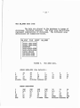
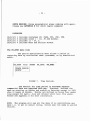
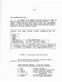
Canadian Technical Report of
Fisheries and Aquatic Sciences 1807
1991
USER 'S MANUAL FOR THE COMMERCIAL SALMON CATCH SPREADSHEET PROGRAM
by
M. A. Holmes and D. W. A. Whitfield
Biological Sciences Branch
Department of Fisheries and Oceans
Pacific Biological Station
Nanaimo, British Columbia
Canada
V9R 5K6
- ii -
(c)Minister of Supply and Services Canada 1991
Cat. No. Fs 97 -6/1807E
ISSN 0706-6457
Correct citation for this publication :
Holmes, M. A. and D. W. A. Whitfield . 1991. User's Manual for
the Commercial Salmon Catch Spreadsheet Program. Can . Tech .
Rep. Fish. Aquat . Sci . 1807 : 44 p .
iii
TABLE OF CONTENTS
ABSTRACT
vi
FORWARD
1
I NTRODUCTION
1
SECTION I
GENERAL OVERVIEW
Historical Perspective
Sa l e s slips
2
2
2
SECTION II
DATABASE STRUCTURE
Ca tch Data System
Structure of the Catch Data
Stratum fields
Effort fields
Species field
Catch fields
SECTION III
PROGRAM USER'S MANUAL
System Access
The main menu
The status line
USER INTERFACE
Overview
Working with the menu
The CDSS menu
G RESTR
COL
ROW
AR SPEC
PR SPEC
DB STAT
FILE
SHEET
OUTPUT
EXEC
QUIT
The DB_STAT menu item
The FILE menu item
PATH
FILENAME
3
4
4
4
4
6
7
8
8
9
9
9
10
11
12
12
16
18
18
18
18
19
19
19
19
19
19
19
19
20
20
20
20
iv LIST
RETRIEVE
SAVE
VIEW
The SHEET menu item
TITLE
SHOW
NEW
GOTO
The
The
The
The
The
The
The
The
COPY
DELETE
AR_SPEC menu item
PR SPEC menu item
G RESTR menu item
Menu selection editinq
G RESTR menu
COL menu item
ROW menu item
OUTPUT menu item
DISPLAY
PRINTED
CGP
SPREADSHEET
EXEC menu item
Consistency Checks and Limitations
QUIT menu item
21
21
21
21
21
22
22
22
22
22
22
23
24
25
25
26
27
28
30
30
30
30
30
30
31
31
ACKNOWLEDGEMENTS
32
REFERENCES
32
APPENDIX A
33
APPENDIX B
35
APPENDIX C
39
APPENDIX D
41
APPENDIX E
44
- v -
TABLE OF FIGURES
FIGURE
FIGURE
FIGURE
FIGURE
FIGURE
FIGURE
FIGURE
FIGURE
FIGURE
FIGURE
FIGURE
FIGURE
FIGURE
FIGURE
FIGURE
FIGURE
1-
2.
3.
4.
5.
6.
7.
8.
9.
10.
11.
12.
13.
14.
15.
16.
······
····
·· ··
·
·
·
·
···
·····
·······
··············
· · ·
·····
·
·
·······
· ··
·
···
· ·· · · · ·
····
· · · · · · · · · · · · · ··
·
· · · ·· ·
· ·· · · ·
····
· · · ·
· · ···· ···· · · · ·
· ··· · ·
Logical Structure of Catch System
Catch Spreadsheet Identification Screen
The main menu.
•
The FILE menu.
The SHEET menu.
The AREA menu.
Time Periods.
The global restriction menu.
Column/Data selection.
The ROW menu.
Example of c olumn/data & nested r ow levels.
The OUTPUT menu.
Northern British Columbia Statarea Map
Southern British Columbia Statarea Map
Report Example.
Sample of SHOW for Report Example.
···
··
·· ·
· ·
·
···
·
··
5
10
11
20
21
23
24
25
27
29
29
30
35
37
41
42
- vi ABSTRACT
Holmes, M. A. and D. W. A. Whitfield.
1991. User's Manual for
the Commercial Salmon Catch .Spreadsheet Program. Can. Tech .
Rep. Fish. Aquat. Sci. 1807: 44 p.
Summary information from the commercial salmon catch
sales slip data are stored for the years 1952 to the present on
the VAX computer at the Pacific Biological Station in Nanaimo,
B.C. The summary data contains information on the salmon catch
by year, area, time period, gear type, and species. Additional
information on fishing effort is also included. A spreadsheet
program has been written to allow users to generate a wide
variety of report tables for their own use both on the VAX or on
a personal computer. This manual describes how to use the
spreadsheet program to obtain the information needed.
Keywords: commercial salmon catch, fishing effort, sales slip,
salmon database, salmonid, spreadsheet program
RESUME
Holmes, M. A. and D. W. A. Whitfield.
1991. User's Manual for
the Commercial Salmon Catch Spreadsheet Program. Can. Tech .
Rep. Fish. Aquat. Sci. 1807: 44 p.
Des renseignements sommaires fondes sur les donnees
provenant des bordereaux de vente des prises de saumon
commerciales sont stockes pour la periode allant de 1952 a
aujourd'hui dans l'ordinateur VAX de la Station biologique du
Pacifique , a Nanaimo, en Colombie-Britannique. Ces donnees
sommaires repartissent les captures de saumon par annee, secteur
geographique, periode de l'annee, genre d'engin de peche et
espece . On y trouve aussi d'autres informations sur l'effort de
peche. Un logiciel tableur a ete con~u pour permettre aux
utilisateurs de produire un large eventail de tableaux qu'ils
peuvent utiliser sur Ie systeme VAX ou sur un ordinateur
personnel. Le guide indique comment utiliser Ie tableur pour
obtenir les renseignements souhaites.
Mots cles:
prises de saumon commerciales, effort de peche,
borderau de vente, base de donnees sur Ie saumon ,
salmonides et tableur.
FORWARD
This document introduces the new user t o the salmon
c a tch data spre adsheet program devel oped by Doug Wh i t f i e l d and
Tony Chumak f or the Dept. of Fisheries and Oceans at the Pacific
Bi ol ogical station under the Scient ifi c Authorit y of L. Lapi.
The comme rc i a l s almon c a tch data system described by Fr ed Wong
(Wong 1983 ) cont a i ns deta iled informat i on on the h i s t ory of the
c a t c h data and the intri cac ies of i ts s tructure. The current
repo rt r epeats s ome materi al because o f procedural updates and in
the interest of background cont inu ity.
INTRODUCTION
The system described here a c c e s s e s t he catch database
(Wong 1 983 ) and produces flexible reports in a generalized
s pr eadshe e t form. Output includes a choice of screen display, a
printable r eport, a standard spre adshe et fil e a nd a file
fo rma t t ed f or input to the PBS Custom Graphics Package (Kuhn,
Wh itfield and Chumak, 1 988). Since most u s ers will use the
program through the Salmon Stock Assessment (SS A) menu on the
comput e r at the Pacific Biological station (PBS) ipr oc edur es for
using the program will be focused on this computer (VAX). When
procedure differs between the VAX a nd micro -computer versions of
the program, these differences will be noted in Appe nd i x C.
section I covers background details on the history of sa les slip
data and the compilation of the PBS catch database . Section I I
explains the structure of the data in the da t a base , whil e Section
III describes the program with various menus used t o format a
report.
- 2 -
SECTION I
GENERAL OVERVIEW
Historical Perspective
As the B.C. fishing industry developed, so did
fisheries regulations and management problems. It was recognized
in the late 1940's that a more accurate and detailed accounting
of fishing catch statistics was needed. Consequently, after
consultation between government officials, industry
representatives and biologists, a report was issued on a mUltiple
sales slip system (Burton 1948). This system was acknOWledged to
be the best method of providing complete and detailed information
on the catch. A trial sales slip system was instigated for the
Nass and Skeena River areas and its success led to the extension
of this system, in 1951, to the remainder of the province.
In 1967, the Block Brothers Computing Centre in
Vancouver (BB) began computer processing and storing 'the catch
data for DFO. Two reports were published annually, but much of
the data was still unavailable for users who could not access the
data in a timely, flexible or inexpensive manner.
In 1981, PBS purchased its first multi-user computer
and the present salmon catch database was designed using the BB
catch tapes. Fred Wong developed the programs and subroutines
necessary for the efficient storage and retrieval of summary
sales slip information (Wong 1983). Catch information on tapes
was sent from the Catch Statistics Division of Fisheries Branch
to the Salmon Information unit of the Biological Science Branch,
where the information was assembled and stored on the PBS
computer.
The original reports that users could access on the VAX
have now been replaced by the spreadsheet program which allows
greater variety in the content of the reports.
-
3 -
Sale. .lip
The data collection mechanism is via the sales slip.
Each time a commercial catch is sold, a sales slips is completed
and a copy sent to Department of Fisheries and Oceans (DFO).
Information on the sales slip, which becomes the basis of the
salmon catch database, is : sales slip number, gear used to catch
the fish, date of sale (or landing), company purchasing the fish,
number of days fished and statistical area of catch, species,
form (round, dressed head on, etc.), number of fish (pieces),
weight and price. The sales slips a re issued when the catch is
first sold, usually at the point of landing. The fish processing
companies collate the data and then forward the slips to DFO for
keypunching. Some companies now enter the data themselves
through an electronic system. The companies manually check the
slips then enter them at their work site. Extensive electronic
checks are made at the time of keypunching. The Remote Saleslip
Entry System (RSE) gathers sales slip data directly via phone
lines. DFO will add the electronic data to their sale slip and
average weight files . Errors identified by DFO's audit must be
corrected by the fish company within three working days. Errors
are minimized by validating such things as the vessel CFV,
species coding, weight ranges etc. The data are required to
reach DFO within seven days of landing the catch.
Keypunching of the sales slips is done by contract
staff who sort the information by gear, area and time period and
manually inspect and correct obvious errors such as incorrect
species codes, month-day transpositions etc.
The biological
sample data (length, weight, age etc.) are used to estimate the
average weight for each salmon species. For a sales slip lacking
information on the numbers of fish, but with weight information,
the number is estimated by dividing the weight with the average
weight of the particular species, area, week and gear concerned.
- 4 -
SECTION II
DATABASE STRUCTURE
Catch Data system
Records of each sales slip reported in a year are
stored on magnetic tape by the Statistics Unit of Fisheries
Branch in Vancouver. These data are then processed by a series
of database programs at PBS. The data may be accessed via the
menu-driven spreadsheet report writer, or by user written FORTRAN
programs. Library routines exist to handle data access for the
user written programs.
Summary catch information by year,
area, time period, gear and species, number of days open and
amount of effort are maintained on the PBS computer. The summary
catch database and spreadsheet report writer may also be used on
an IBM compatible micro-computer. Annual catch data are usually
finalized by October of the year following the reported catch.
structure of the Catch Data
In order to understand the catch data, it is necessary
to know something about the salmon fishery. Salmon are caught
near the coast by commercial fishermen. The fishery can be
broken into sub-units which expedites management of the many
separate salmon stocks. An individual fishery encompasses both a
restricted geographic area and time period. Thus, to describe
the catch requires the definition of this spatial-temporal unit
which we refer to as the catch stratum. This stratum represents
the highest resolution of spatial-temporal information obtainable
from the spreadsheet program.
The catch stratum has four components, the year, the
time period, the fishing area and the fishing gear. While the
year and fishing gear have conventional definitions, the time
period and area use specialized terms. The basic unit used to
delineate the time period is the statistical fishing week (or
stat week) which is explained by example in Appendix A. The unit
used to delineate a basic geographic area is the statistical
fishing area (stat area). These areas are described and shown in
Appendix B as part of the catch region list. The use of the word
- 5 -
"statistical " in these terms comes from their association with
the catch statistics group within DFO.
The sales slip data are summarized by catch stratum
(i.e. year, statarea, statweek and gear) in the database used by
the spreadsheet program. Information about individual vessels or
individual landings is available on the detailed annual sales
slip magnet tapes but the data are totalled for an individual
catch stratum in the database. Information about larger units is
generated by combining the catch strata into groupings
representi ng wi de r boundaries of space , time, gear, etc. Some of
these groupings can be done automatically by selection of the
appropriate spreadsheet menu item . For example, groupings into
catch region (catch regions usually incorporate several stat
areas) is a potential menu choice . Thus, the program generates
all information about uni ts larger than a single stratum by
summing over the appropriate strata and related information.
STRATUK
1- Year
2. Ar e a
3. Time
4.
Gear
Period
SPECIES
8.
Species
(grade)
EFFORT
5.Days
Open
6.Days
7.Number
Fished of Boats
CATCH
9.pieces
10. Total 11 . %Dressed 12.Average
Weight
Price
FI GURE 1.
Logica l structure of Catch System
- 6 -
The logical relationships of the data fields in the
database are graphically shown in Fig. 1. In the figure, the 12
separate data fields have been combined into four groups of
related information. For example, the top box in the figure
contains the four data fields that together define the catch
stratum. Fields which are numbered and listed within a box are
independent of one another. Thus, the year and area fields both
help define the catch stratum and are independent of each other.
A catch stratum is defined by choosing a single value
for year, area, period and gear i.e. 1984, statarea 1, statweek
061, and seine net. If more than one value is chosen for any of
these four fields, for example, the statareas 1 & 2, then there
is no longer a single catch stratum, but, in this example, two
catch strata which could be summed together or reported
individually depending on the report choices.
The two boxes on the second level rely on the
additional information above them to be interpreted properly.
This hierarchial relationship is depicted graphically by the
vertical lines connecting the boxes. For example, the second
level in the figure includes the effort box, therefore, the
effort fields contain information appropriate for the selected
catch stratum. Finally, the lowest level contains the catch
fields. These fields report information that applies to the
combined catch stratum and species selections, but does not need
the effort data to be interpreted properly.
stratum fi el ds:
(These fields delineate when and where the
fishery occurred.)
Year - The year the landings were made. The catch
spreadsheet program starts with 1952 and includes data
up to the most current year of available information.
Period - The time period is a subset of the total group of
statistical weeks, plus one additional period which
includes several statweeks (Appendix A). statweeks are
written as a three digit number, with the first two
digits delineating the month and the third digit giving
the week wi t h i n the month. statweeks 031 through 114
are a ll included individually within the catch
database. The additional period, statweek 120, is
defined as all statweeks not included individually
above, i.e., statweeks 011 through 024 plus 121 through
124. Prior to 1969, the months of March and April were
reported by statistical month.
- 7 -
Area - Data are stored by statarea (see Appendix B). Note
that other area types, such as catch region, are
available. Catch regions are defined as a combination
of statarea and gear type. For some years some
statistical areas were divided into subareas and data
is reported by subarea when available. Care should be
used when using subareas since they will not
necessarily total to statarea.
Gear - Four different gear types are specified: troll,
freezer troll, gill net and seine net. Day troll boats
and ice troll boats are combined in the troll
category, while freezer troll is segregated into a
category by itself.
Bffort fields:
(These fields describe the fishing effort
associated with a catch stratum).
Days Open - The number of days the fishery was open for
fishing. This information is not currently available
at this time, however, space for the data has been
reserved.
Days Fished - This field and the next report information
related to fishing effort. The interpretation of this
field is conditional on the gear type. Specifically,
for troll boats, the field reports the total number of
boat days fished by strata. For net gears, the field
represents the total number of landings by strata.
These data are only available from 1963.
Number of Boats - This field represents the number of boats
making at least one landing within a statarea, statweek
and gear stratum. Thus, it has two possible
interpretations, one of which is meaningful only for a
single catch stratum.
These interpretations are:
1). For troll, as a measure of fishing effort, the
number estimates boat trips. This definition is still
valid when several strata are combined.
2). This field estimates the number of boats
participating in the fishery represented by the
stratum. This definition may not be valid when several
strata are combined, because double counting of boats
can occur. There is no number of boats data from
1952 - 1967 in the database.
- 8 -
specie. field:
(This field selects the species within the catch
stratum).
Species - The six species of Pacific salmon, chinook, coho,
chum, pink, steelhead and sockeye are all included. In
addition, chinook grade types are included as though
they also represented separate species. These grade
types are: large red (>12 lbs.), medium red (8-12
lbs.), small red (1-7 lbs.), #2 red «7 lbs.), whites,
and jacks «5 lbs.). Selecting large red results in a
summary of all red chinook over 12 pounds. The choice
of chinook gives the totals for all chinook grades.
Note that the grade types apply only to chinook.
Catch fields:
(These fields describe the catch within the
selected catch stratum and species composition).
Pieces - The number of fish landed.
Total Weight - The total weight of landed fish. Total
weight can be reported in either pounds or kilograms at
the user's discretion. This field is conditional on
gear type, since the different gear types use different
weight standards. Troll fish weight is reported for
fish dressed with head on, whereas, for net caught
fish, the standard assumed is for round weight (head
on, undressed).
% Dressed - The percentage of landings landed as dressed
weight rather than round weight. The program
compensates for troll landed head off with an algorithm
than adjusts to dressed head on. This data is
available in 1973 and from 1982 on.
Avg Price - The average price paid for the fish.
Price can
be reported in either price per pound or per kilogram,
at the user's discretion. This data is available from
1972 on.
SECTION III
PROGRAM USER'S MANUAL
A spreadsheet is produced by working interactively with
the program and making choices from menus. An interpreter
accesses the catch database and then generates the output either
interactively or in a batch process. In one session several
spreadsheets may be specified, and these specifications may be
saved to and restored from disk.
system
AeC8S
CDSS can be run either on the VAX at PBS or on a microcomputer with sufficient disk space and memory. While many
micro-computers are self-sufficient, DFO uses them to also
emulate a terminal on the VAX, where software enables the user to
logon directly into the mini-computers while still being on the
micro-computer. Details on how to log onto the VAX can be
obtained from the computing Division at PBS.
To begin the interactive spreadsheet program on the VAX
enter SSA C for Salmon Stock Assessment (SSA menu) - Salmon
Catch Database being selected (C):
IDAFfY>SSA C
- 10 -
14-0ct-1990;
9:53am
user: Salmon
sunday
CATCH DATABASE SPREADSHEET SYSTEM
Version 3.3
copyright 1989, Government of Canada
Department of Fisheries and Oceans
L---------Press any key to continue---------.....
FIGURE 2.
Catch Spreadsheet Identification Screen
The introductory screen provides information on copyright,
date and time of report production (Figure 2).
The main menu
For the rest of the interactive session, the main
display window contains the main menu at the top and a status
line at the bottom (Figure 3). Each menu choice will be
explained in detail.
-
11 -
DB STAT FILE SHEET AR_SPEC PR SPEC G RESTR COL ROW OUTPUT EXEC QUIT
F2: Help
Sheet 1 of 1
F4: Redraw Screen
Path: \CATCH\CODE\
FIGURE 3.
File: setfile
The main menu.
Note: The order of menu items is not the order in which a report is created
i.e. DB STAT Is the first item on the menu but it only gives information on
the dat~base, while G_RESTR is used to format the contents of the report.
The status line
The status line at the bottom of the main menu screen
gives information on help keys, directory or path, filename and
spreadsheet number. It provides information on help (PP2) and on
refreshing the screen (PF4), as well as the name of the report
(default file name is settile), where the report is being created
(Path: [OSBRNAMB]) and which report is currently being worked on
(Sheet 1 of 1). All of these items will be discussed in the
following sections.
- 12 -
USER INTERFACE
This section describes the interactive program and how
to produce a report. Read through this section briefly to get an
idea of the choices to be made and then go to Appendix 0 to work
through an example. This will produce a simple report so that
the documentation that follows will be more meaningful.
overview
A spreadsheet program creates a table of numbers
arranged in rows and columns. The columns are the "vertical"
lines of numbers, while the rows are the "horizontal" lines.
Thus, in the table
1
4
2
5
3
6
the first row contains the three numbers 1, 2 and 3, while the
third column contains the numbers 3 and 6. Such a table is often
a useful way to organize complex data, especially when different
rows and columns represent different facets of the data. For
example, if, in the above table, we wanted to show the number of
children enroled in grades 1-3 by the sex of the child, we could
write
Numbers of children enroled in school
Girls
Boys
Grade 1
Grade 2
Grade 3
1
2
5
3
6
4
Now our table is much more meaningful. In this trivial example,
we have constructed a table containing numeric data which was
organized in a logical way and becomes easy to interpret by the
appropriate use of row and column labels.
The COSS spreadsheet program allows the user to
construct tables whose entries report on the commercial salmon
catch in B.C. To organize a table in a meaningful way, the user
must decide what information is wanted in the rows and columns
of the table, and what labels are associated with rows and
columns. Therefore, the first distinction we want to make is
between the data reported in the table (the numbers themselves)
and the column or row labels (a category of information). In the
- 13
~
example above, the data are the actual numbers of boys or girls
in a specific grade. The categories are grade and sex. The
position of a number in the table indicates that it belongs to
the respective row and column categories. Thus, of the five
students in grade 1, four are boys.
A more complex, but more relevant, table generated from
the COSS program is shown below:
10
74
Pieces
Troll
STWK
Gillnet
STWK
STWK
STWK
STWK
STWK
STWK
STWK
061
062
063
064
061
062
063
064
75
Pieces
12
74
Pieces
75
Pieces
----------~---------~~----------~---------------
0
116
703
2627
0
0
0
0
126
656
375
1087
0
0
0
0
991
1738
10626
6791
0
95
1000
5926
941
1111
1672
2426
33
297
2194
5564
This table reports the numbers of salmon (pieces)
caught within each week for a four week period, over two years,
in two statistical areas, by two types of fishing gear. Only one
item in this list represents the data displayed in the table , the
pieces. All other items in the list are category labels for
either rows or columns.
Let us first examine the column labels. There are
three levels of labels for the columns of the table. The upper
level represents the statistical areas selected by the user for
the report, areas 10 and 12. The next level represents the years
selected by the user, 1974 and 1975. The final level of
labelling is not a label at all, in the terms of COSS, rather it
is the name of the data type reported in the column, pieces.
Notice that the middle level of labelling, years, is nested
within the upper level, statistical areas. Therefore, since two
areas have been selected, each year label is repeated twice, once
for each area. All of the numbers in the first column satisfy
both levels of label categories, that is, they represent numbers
of salmon caught in area 10 in 1974. Likewise, all of the
numbers in the last column represent numbers of salmon caught in
area 12 in 1975.
- 14 -
The rows in this table have two levels of labels, gear
and statistical week. Like the columns, the row labels are also
nested. Thus, the first four rows report on separate statistical
weeks for troll caught fish, while the next four rows do the same
for gill net caught fish. The combination of row and column
gives the individual entries i n the table their unique meaning.
For example, in area 10 in 197 5 the troll fleet caught 1087
salmon during statistical week 064.
In addition to reporting the da ta selected by the user,
t he COSS progr am can also provide row or column totals. This is
often a useful feature . However, be wa r ned that selection of
t ot a l s can lead to a substantial increase in the size of the
t able produced. For exampl e i f we select t he option to produce
tot a ls f or both rows and columns f or t he above table, the
r e SUl t i ng t abl e i s:
10
76
PI K
ItS
75
Plec:"
TOTAL
12
74
Pieces
Pieces
•••••••••• ••••••••••••••••• ••••••••••••• 0
Troll 51\1: 061
0
ST\IIC 062
116
063
703
STY!( 064
TOTAL
STW: l)j)1
2627
$ 1\1(
Gill
t
SM
TOTAl
062
063
3446
0
0
0
0
ST
ST OM
TOTAL
ST\IIC 061
STWK 062
0
116
STt« 063
703
0
STh'!( 064
2627
TOTAl
3446
126
656
375
1087
2244
0
0
0
126
rn
1078
3714
5690
0
991
1738
10626
6791
20146
0
95
0
1000
5926
7021
991
1833
11626
12717
27167
0
126
656
375
1087
2244
126
0
rn
1078
3714
5690
Pi ece
TOTAL
TOTAL
74
75
TOTAL
Piec es
Pieces
Pieces
Pieces
•••••••• ••••• •• ••••••••••••••• ••••• •••••••• -
0
0
0
75
941
1111
1672
2426
6150
33
297
2194
5564
8088
974
1408
3!66
7990
14238
1932
2849
12298
9217
26296
33
392
3194
11490
15109
1965
3241
15492
20707
41405
991
1854
11329
9418
23592
0
95
1000
5926
7021
991
1949
12329
15344
30613
•••••• •
--- •••••• •••••••
1067
1767
2047
3513
8394
33
297
2194
5564
8088
1100
2064
4241
90n
16482
2058
3621
13376
12931
31986
33
392
3194
11490
15109
2091
4013
16570
24421
47095
~
15
=
The table has increased from 4 columns to 9 and from 8
rows to 15. Totals are shown for both levels of row and column
labels. For example, 2849 fish were caught by troll in area 12
during statistical week 062 for the years 74 and 75 combined,
while 3241 fish were caught for the same week and same area when
troll and gill net gear categories are combined.
The final feature of the COSS program to discuss in
this overview is the concept of restriction. The tables for
salmon data shown above were created by restricting the range of
the row and column categories. For example, the years were
restricted to just 1974 and 1975. If no restrictions are made
for a label category, all the information for that label will be
included. Thus , no restrictions on years would result in summing
the data selected over the entire range of years contained in the
database. Therefore, the process of restricting the label
categories to select the information relevant to the user, is the
key to using the program to create meaningful tables.
As an example of the combination of restriction and
label selection, consider the table below.
Pieces
STWK 061
STWK 062
STWK 063
STWK 064
2091
4013
16570
24421
To produce this table, the same restrictions on year,
period, area, gear and species were selected as for the t~o
previous tables. What was not selected was two levels of row and
column label categories. Therefore, instead of reporting areas
separately, they have been pooled. The same is true for years
and gear types. Comparison of this table with the previous one
shows that the pieces reported here match that portion of the
previous table for which totals have been made over areas, years
and gear types.
- 16 -
Note that by not segregating areas, years and gear
types, the table is not well documented. Just by looking at this
table, there is no way to tell that the catch from only areas 10
and 12, years 1974 and 1975 and gear types troll and gill net are
being shown. To help with this problem, COSS also prints a
summary of the selections made by the user for every report
generated. The summary for the above table is:
Sheet 1 of 1
Created 14-Kar-1991 ll:26am
Title:
Area spec: STATS AREA-SUBS Period spec: STATS PERIOD
Selected years:
74 7S
Selected areas: 10
12
Selected periods:
S'NK 061 S'NK 062 S'NK 06·3 STWK 064
Selected gear:
Troll
Gillnet
No species restriction
Selected data:
Pieces
Veight unit
Kg
Veight not corrected for % dressed
Cols: l:none
N 2:none
N
Rows: l:PERIOD N 2:none
Output: PRINTED
N 3:none
The combination of the table and the summary provide sufficient
information to properly interpret the output from COSS.
wortinq witb tbe menu
The user makes choices through horizontal and vertical
menus. The general procedures for moving through these menus is
described before discussing the formation of the spreadsheet.
An entry can be chosen by typing the first letter of
the entry (i.e. File or Screen) or by using the arrow keys to
move to the item of choice and then hitting <Inter> ( or
<Return». Where menu items begin with the same letter, the
cursor goes to the first occurrence of that letter.
The main menu is displayed in one line across the
screen top. Sub-menus are arranged one item above the other in
boxes near the top left corner of the screen.
N
- 17 -
Here are some quick tips for working with text within
the menus.
[PF2] - is the help key.
[PF4] - refreshes the screen if it becomes corrupted.
<\>
- backslash key steps user back out of submenus.
Note: the arrows move along a line but not down unless you press the down
arrow.
->
<-
<Ctrl-B>
<Ctrl-E>
<Ctrl-G>
<Ctrl-H> or
<Delete>
<Ctrl-D>
<Ctrl-I>
<ctrl-Y>
move within string.
move to beginning of string
move to end of string
delete character to right of the
cursor
delete character to the left of
the cursor
delete to end of line
toggle insert/overstrike mode
(abort) will work at a logical point
in the program i.e. between sheets
while <Ctrl-C> will return to the
VAX prompt immediately.
Note: \ is used to step back out of the sub-menu. However <Return> or
<Enter> are used when a choice has been selected. If these are not used, the
program cannot handle the unexpected response and it will abort.
- 18 -
The CDSS .enu
First, let us take a look at the types of operations
the user performs by using the CDSS menu. The following three
menu items determine the contents and layout of a spreadsheet
report:
G RESTR
- Global restrictions. This menu item lets
the user choose the appropriate subset of
information in which he is interested. The
data fields that can be restricted are all
four stratum fields (year, area, period and
gear), and the species field. For example,
the user might be interested only in the
years 1964 and 1982. He would then select
only these years using the restriction
procedures described below.
COL
Column definition. There are two types of
choices for definition of the column entries.
The first is the type of data to be shown in
the columns of the report. The data items
are all from the catch fields of the
database. The second choice is referred to
as "sort level" and determines the label
categories for the data. For example in the
overview, the data selection was pieces,
while the label categories were years and
areas. Label categories all come from the
stratum and species fields.
ROW
Row definition. The row definition is
similar to the column definition, with the
exception that no data selection is involved.
Therefore different rows of the table
correspond to different label categories. In
the overview example, the row label
categories were gear and periOd. Row labels
also come from either the stratum or species
fields of the database.
- 19 -
The next two menu items let the user specify the units
of measurement defining the area and time period.
Area specification. The user chooses from
the various types of areas the program
supports. For example he may choose
statistical areas or catch regions.
Period specification. The user chooses
either statistical weeks or statistical
months as the time period units.
The last menu items select I /O options, report on the
current status of the database, execute the program commands or
return to the operating system.
Database status. Reports on the current
status ot intormation in the database.
FILE
File specification. Lets the user name,
save, retrieve and view CDSS files.
SHEET
Spreadsheet name. Allows more than one
spreadsheet to be constructed during a single
session of program use.
OUTPUT
Program output. Lets the user decide what
type of output he wants.
Eue
Execute. Instructs the program to execute
the commands built up by the user to produce
the spreadsheet.
QUIT
Quit the program. Returns control back to
the operating system.
We shall now go through each of these menu items in
detail and describe all of the relevant features.
- 20 -
For the entire database the status is:
1) the latest year of data available,
the number of years of preliminary data,
the years for which days-open data are
available (99 - not available),
4) descriptive text on data.
2)
3)
The FILE menu item
This submenu provides information on the files in the
current directory and allows the retrieval or storage of
spreadsheet specifications (files with the extension of .SET ).
PATH
FILENAME
LIST
RETRIEVE
SAVE
VIEW
FIGURE 4.
The
FILE menu.
PATH - this allows a path or directory to be changed
from the default directory in which the user is working
to other directories.
FILBHANB - the default file name is SETFILE and
extension choices are described in Appendix E. A
unique filename can be chosen here.
I,
- 21 -
LIST - allows listing of files in the current directory
defined by PATH . Save sets, the files in which
spreadsheet specifications are stored have extension
' . s e t' . I f LIST i s selected, all of the filenames
from the current directory are listed. Selecting
USER_ F I LES results in a prompt for the desired filename
e xtens i on i . e . t o list a ll of your .com files, erase
the * a nd ente r c om.
RBTRIBVB - c hoosing this wi l l show a menu of all file
names wi th t he extension . SBT from the current
d i r ectory; a fi le can be selected from the list by
mov ing over t o i t via a rrows and hitting <RETURN>.
whe n saving a f ile , the user is prompted for a
fil e name . I f a name ha s al ready been entered under
PI LENANB t hen moving to SAVE will save it under that
f i l e na me.
SAVE -
VI EW - d i s pl ays the same list of .SBT filenames as does
RETRIEVE. Lets the user see the files but not retrieve
them.
The
sniT
nu itWil
The SHEET s ub - me nu provides control over the sheets in
a set. During an interactive session, more than one spreadsheet
can be s pe c i f i e d with NEW . A single s p r e a d s he e t specification
is called a sheet, a nd the collection of sheets from one session
is a set .
DB STAT
FILE
SHEBT
TITLE
SHOW
NEW
GOTO
COPY
DELET E
FI GURE 5.
The SHEET menu .
- 22 -
TITLB - prompts for character string to form title of
current sheet. Up to 50 characters can be chosen.
SHOW - displays information on the current sheet.
NEW - adds a new, empty sheet to the set. Note sheet
number in the bottom left hand corner of the status
screen. The maximum number of sheets is 10.
GOTO - prompts for the number of a sheet which then
becomes the current sheet. This facilitates moving
around a report with many sheets.
COpy - prompts for the sheet number where contents are
to be copied to the current sheet. i.e. If the user
has made the first sheet (report) then creates a new
spreadsheet with NEW, COpy allows information already entered
for one sheet to be copied to another sheet. This is very
useful when many aspects of each sheet will contain
similar information.
DBLETB - removes a sheet from the set.
- 23 -
The AR SPBC
enu it
The data are stored in the database in terms of
statareas, including subareas. The other area definitions
represent combinations of statareas. The different area
definitions are summarized below.
DB_STAT
FILE
SHEET
AR SPBC
STATS AREA-SUBS
STATS AREA+SUBS
DISTRICT
DIST+STATS-SUBS
DIST+STATS+SUBS
CATCH REGION
CR+STATS-SUBS
CR+STATS+SUBS
FIGURE 6.
STATS
1
2E
8
9
17
16
24
Alaska
ARn~SOB
25
Taku
The AREA menu.
(the default):
2W
10
18
26
stikine
3
11
19
27
Unknown
4
12
20
28
BC
5
13
21
29
6
14
22
30
2AW
5/2
11
19
27
Alaska
2BW
5/3
12
20
28
Taku
3X
5/4
13
21
29AB
Stikine
3Y
6
14
22
29C
Unknown
7
15
23
C
STATS ARBA+SUBS
1
4
8
16
24
29E
2AE
5/6
9
5/1
10
17
18
25
30
26
C
2BE
3Z
7
15
23
290
Be
-
24 -
CATCH REGIONS ( t hose geographical areas combing with gear) .
Please see APPENDIX B fo r catch regio n summary :
DISTRICTS
District
Dis trict
Distric t
Distr ic t
1 includes statareas 28, 29AB , 29C, 29D, 29E.
2 i ncludes areas 1 - 10 , 30 and Alaska .
3 i nc l udes 1 1 - 27 , C.
4 i nc ludes Na s s a n d St i kine Rivers .
The PR SPEC menu item
The per iod specification menu a l lows a choice of
repo rti n g d a t a by statistical we ek (statweek) or by statistical
month.
DB STAT
FILE
SHEET
AR SPEC
PR SPEC
~~~;~-~~~~~~]
MONTH
-- ----------
FIGURE 7.
Time Periods .
The default for time period is statweek because
commercial data are reported this way.
Statweek defi nes the
we e k as s t a rt i ng on Su nday and ending on Saturday except in 1981
whe n i t bega n on Mond a y.
Months are defined as being four weeks
l ong e xcept for April , July and October which have five weeks.
Please see Ap p e n d ix A for mo r e information .
NOTE : The p rogram will sum all the data if no restrictions are
ma d e i .e . to get an annual rollup , choose year but make no period
choices~
- 25 -
Ifhe G RBSTR
enu i tea
In Figure 8, the global restrict i on me nu i s shown and
gear has been chosen to be defined f rom t he sub-menu . The
global restrictions menu defines the co ntents of a spreadsheet
report . Salmon catch by year, period , area , gear and s pe c i e s
along with units of weight and weight co r rections may e ac h be
limited to the user selected values.
DB STAT
FILE
SHEET
AR_SPEC
PR SPEC
G RBSTR COL ROW OUT
Troll
Gillnet
FIGURE 8.
The gl obal restriction me nu.
The following section explains the small editor
available within the menu selection box.
Menu selection editing - This box contains
information for manipul ating t he da ta choices .
\ = Quit
T = Top
B = Bottom
C = Clear all
A = Select all
8
S leot
=
-
makes no choices .
to goto t he t op of t he screen .
move t o bottom of screen .
cl ears a l l previous chosen
selections.
- t o choose al l data choices .
- Bit S to begin selec tion .
-
26 -
U - UnSelect
- Hit U to unselect data.
PFl - Toggle [S or UJ - can use this to move among data
selecting and unselecting
i.e. choosing chinook and
coho in SPECIES.
<Return> = Finished selection - selects data chosen
with 8.
Use ARROWS to move cursor to data.
NOTE: Quit is the backslash (\) and no restrictions would be chosen.
restriction Is made then <RETURN.> should be used.
G RBSTR menu:
below.
If a
The individual menu items are described
Year Period -
Data from 1952 available.
choose the week (s) or month(s) which will
define the report .
Area choices can be either catch region,
statareas , subareas or districts.
Gear the gear choices are troll or freezer troll,
seine and gillnet.
Species - Chinook includes the totals of the other
chinook grades.
wgt_unit- Kilograms (default) or pounds.
corr_wgt- For troll the standard weight is dressed head
on. This option will convert troll to round
weight which is handy for comparing the total
tonnage between troll and net. Default is
weight not converted to round weight for
troll (N).
There is a connection between gear and area when area
is chosen as CATCH REGIO.. Catch region by its definition
describes a geographical area and gear. Catch regions are used by
MRP for sampling purposes.
If catch region Northern Net (NN)
were chosen as the area and troll as the gear, a spreadsheet with
no data would be produced as NN is by definition an area for net
gears.
~
27 -
COL or column defines the vertic al a s pect o f the
spreadsheet. Coluxm divides its Information between dependent and
Independent variables. Dependent variables are da ta and Independent variables
are sort levels . Data (dependent) variables a r e : pieces, total
weight, percent dressed weight, average wei ght , pieces per day
f ished, weight per day fished , number of boat s , days fi shed ,
average price and landed value as you c an s e e from Figu re 9.
Some of the dependent quantities listed, i.e . average weights,
are calculated.
DB_STAT
FILE
SHEET
AR SPEC
PR SPEC
G RESTR
COL
ROW OUTPUT
EXEC
I
FIGURE 9.
Column/Data s el ect i on.
In t he example above, COL/DAT has be en se lected and
the DAT s e l e c t i on box shows choices avai lable f or report
select i on . DATA de f i nes the numbers shown in the column(s) of
the spreads he et as ~
PIECES TOTAL WT
=
%DRESSED_WT AVG=WT =
PIECES/ DF WEIGHT/DF NIDi BOATS DAYS_FISHDAVG_PRICE LANDED_VAL -
the actual number o f fish caught .
weight undressed, head on.
, of fish out of the t otal l an ded that
were dressed.
weight/pieces. *
days fished/pieces .
weight/days fished.
i of CFV landings by area by s t atwee k.
Days fished for troll, landings for net.
Average price by weight .
Total landed value
- 28 -
• Weights for troll are dressed with head on, and for
net are round weight. Collection of average weights information
from the MRP commercial sampling program, enables the estimation
of species and gear specific average weights. The MRP data is
provided in a file by area, gear, period, and species and each
record contains the number of fish sampled and average weight per
fish. This information is supplied by the MRP data entry
contractor, to Catch Statistics in Vancouver because these values
are more accurate than those found in the average weight table
generally used for editing purposes.
Independent variables (sort levels) are: year, period,
area, gear and species. Column contents depend on the data
items. Sort levels are used in columns to help specify
categories of data of interest to the user. For example, the
user may select pieces as the data item, and year as a sort
level. This choice would result in one column per year for the
years specified using G_RESTR. Each column would have the pieces
caught in the corresponding year. If no sort levels are chosen
i.e. from 1ST_LEVEL or 2ND_LBVEL, the spreadsheet columns will
become the data variables. Each sort level chosen after data
variables are chosen, mUltiplies the number of values taken by
that independent variable.
The ROW menu item
Spreadsheet rows are determined by one, two or three
nested sort levels. A spreadsheet without at least one row sort
level has no meaning, and this will generate an error message
when the report is run. The number of rows in a spreadsheet are
the product of the number of values taken by each sort level
variable (plus one if summation [TOG_TOTAL] is specified).
I
1.
- 29 -
DB STAT
FILE
SHEET
AR_SPEC
PR S PEC
G RESTR
COL
ROW
1st LEVEL
2nd:LEVEL
3,...------,
SYEAR
-
PERI OD
AREA
GEAR
SPECIES
TOG_TOTAL
<----:::l
SOB-HEW
~
CLEAR
FIGURE 1 0.
The ROW menu.
In the examp l e below, 1ST LEVEL chosen was area, while
2ND L!lWL chosen was species . No t e that the row sorts from the finest
detail of da ta (ar ea) to the least detai l (spec ies ) whi ch is the reverse of
most spt:e dsheet 1 yout:« .
TOG_TOTAL will add the total. of •
particul~r
1 v 1 in another ro
ex pI
unchosen.
CLEAR r emoves previous c ho ices and leaves the level
0
but was not chosen i n this
Th e column choices were PIECES for data and the
1ST LEVEL wa s YEAR.
I
Sheet
Chinook
1
NTR
SWTa
NN
SWVN
Chum
NTR
SWTR
NN
SWVN
FIGURE 11.
17 96 65
327853
5 0 7 67
48313
61559
1349
857189
187117
186723
2797 69
70667
21263
14 6935
44929
1019126
1616890
1529 99
26 1103
427 16
4 115
50750
52510
626966
387679
177457
265787
4 1245
612
62135
3123
37 1389
395446
Example of column/data & n e ste d row l e v els .
- 30 -
The OUTPUT .enu i t_
The output from CDSS is available in several forms.
Interactive output of the spreadsheet will appear as a table of
rows and columns on the computer screen. A larger spreadsheet
can be viewed by scrolling. The cursor control arrow keys will
cause movement by one row or column in the direction of the
arrow. The keys <u>, <d>, <1> and <r> will cause the spreadsheet
to move by one screen in the up, down, left and right directions
respectively.
SELECT OUTPUTS
DISPLAY
CGP
SPREADSHEET PRINTED
- - - - - - - - - - - - - [ Move ] - - - - - - - - - - - - = Quit, T = Top, B = Bottom, C = Clear all, A = Select all
Use ARROWS to move cursor, <Return> = Finished selection
S - Select, U = UnSelect, PF1 = Toggle [Move]/[S or U]
I
FIGURE 12.
The OUTPUT menu.
DISPLAY - the spreadsheet will appear on
the screen where it may be scrolled for viewing.
PRINTED - This choice is the default output method.
The spreadsheet will be written to a file for
subsequent printing on a 132 column printer.
Spreadsheets too large for one printed page will be
split over as many pages as necessary.
COP
- creates a data set that can be imported into the
CUstom Graphics Package by B. Kuhn (Can. Tech. Report
No. 1659). The program contains a stand-alone program,
specifically designed to interface the the MRP*Reporter
program.
SPREADSHBET - will generate files which are formatted
for input to a standard spreadsheet.
The BXEC menu ite.
The execute menu offers a choice of interactive or
batch processing. The default Is Interactive which processes the
- 31 -
spreadsh ee t as y o u wait. Jobs can al s o be sent to the batch queue on
t he VAX which will free up your t e rminal to do other work.
GO - submits job t o bat ch queue on the VAX or to
i nt e r act i v e s creen depe nd i ng on which choice has been
made i n DEVICE .
DEVICE - defines how the j ob wil l be run . Short (CPU
t ime of 3 mi nutes or less ) batch queue (S g B), long
batch queue (more than 3 minus t e s CPU t i me to run), the
interactive screen (will run immediately from the
s creen at the GO c ommand) or CREATB_JOB_ FILE which
creates a batch file (.COM extension) to be submitted
to any queue at a not he r t i me. Several different file
extensions are c r e a t ed depend i ng on what output files
are chosen and also on how the job is run. See
Appendix E for details.
BE_USER - for use by SSA group only .
c ons i s t e ncy Check~ and Limi tations: When the GO sub-menu
item is selected under EXECUTB, then a set o f consistency checks
is d one on the spreadsheet specific at i on s which the user has
This is done sheet by sheet, a nd t he user is
e sta bl i s he d .
prompted for i ns t ruct i ons to conti nue after each sheet has been
chec ked . If a problem is found i.e . no DATA selection was made
or the same sort level was made in both COL and ROW , a warning or
e rror condition is generated . When a ll sheets in the set have
been checked g the pr ogram checks f or warning or error conditions
and will displ ay a prompt on whether or not to proceed with
processing . usua lly the user would choos e not to p roceed until
the problem has been corrected .
Users who d i s c ove r combinations o f specif ications which
result in erroneous spreadsheets but for wh i c h t he p rogram issued
no warning or err or messages should r eport them to the system
maintenance person so the program can be modi fi ed appropriately.
Th
gUIT
~eDU
item
To exit the spreadsheet sel ect QUIT and reply 'yes'.
- 32 -
ACKNOWLEDGEMENTS
I would like to thank Dr. T. Mulligan for providing
very helpful editorial advice along with perspectives from Brian
Moore, Don Radford, Gail Hudson, Terry Calvin and Sue Lehman.
REFERENCES
Burton, G.L. 1949. Fishery statistics of the Pacific coast
Canada : a report to the Dominion Department of Fisheries
and the Dominion Bureau of Statistics.
Canadian Department of Fisheries and Oceans (DFO). 1951. British
Columbia Catch statistics by area and type of gear.
Chumak, Tony and D.W.A. Whitfield. 1989. PC screen and
keyboard I/O system. Report produced under this
contract.
Kuhn, B.R. 1988. The MRP-Reporter program: A data extraction and
reporting tool for the Mark recovery Program database. Can.
Tech. Rep . Fish. Aquat. Sci. 1625: 145 p.
Kuhn, Brian R., D.W.A. Whitfield and Tony Chumak. 1988. The
CUstom Graphics Package: a Pascal programmer's
graphics toolbox and data presentation system.
Canadian Technical Report of Fisheries and Aquatic
Sciences No. 1659.
Whitehead, Valerie. 1990. Commercial Catch statistics System,
Workflow, Procedures, and Data. Dept. of Fisheries & Oceans
in-house document.
Wong, F.Y.C . 1983. Historical salmon commercial catch data
system of the Fisheries Research Branch, Department
of Fisheries and Oceans, Pacific Region. Canadian
Techni ca l Report of Fisheries and Aquatic Sciences
No. 1156.
- 33 -
APPENDIX A
statweeks are labelled by a three digit code. The
first two digits delineate the month and the last one specifies
the week within the month. Each statweek in the catch database
has 7 days and each month has 4 statweeks except that months 04,
07 and 10 each have 5 periods. Statweek 120 in COSS is defined
as all periods from December through February, inclusive.
The table below for 1975 gives the week ending day and
the statweek (MMW). A table for any year can be generated by
running:
$run ssa:[CWTSYS.TABLES]MMWTAB
Running this program will produce statweeks for all
periods from January but CDSS uses dates from March 1st through
Nov. 30th.
ENDING
DAY MON
YR
STATWEEK
031
032
033
034
08
15
22
29
03
03
03
75
75
75
75
05
12
19
26
03
04
04
04
04
05
75
75
75
75
75
041
042
043
044
045
10
05
05
05
05
75
75
75
75
051
052
053
054
06
75
75
75
75
061
062
063
064
07
07
07
07
08
75
75
75
75
75
071
072
073
074
075
11
24
31
07
14
21
28
05
12
19
26
02
OJ
06
06
06
- 34 -
09
16
23
30
08
08
08
08
75
75
75
75
081
082
083
084
06
13
20
27
09
09
09
09
75
75
75
75
091
092
093
094
04
11
18
25
01
10
10
10
10
11
75
75
75
75
75
101
102
103
104
105
08
15
22
29
11
11
11
11
75
75
75
75
111
112
113
114
75
120
OEC,JAN,FEB
APPENDIX B
-
35 -
.+
Canada
STATISTICAL AREA MAP
SHOWING AREAS OF CATCH FOR
BRITISH COLUMBIA WATERS
NORTHE RN HALF
e:
10
:
<l
,
,
:
..
10
:
:
. 'lOW' . '
'",
10
,
'I'
'",
llAuTlCAl. lll'l.U
N
106
142
10 7
108
~::....-__109
130
-I
110
III
127
SIXTH EDmON Fel '~
FIGURE 13.
Northern British Columbia statarea Map
r-,
(V)
••.•-
III
127
- -- - - -_ .
._---_ -.!......_ -- ~.
~~~
.+
and Oceans
F.sheroes
at Oceans
Pilches
Canada
STATISTICAL AREA MAP
0
! !
~
:
!
~
!
~
IULOIIf. 'q, a
lO
SHOWING AREAS OF CATCH FOR
BRITISH COLUMBIA WATERS
SOUTHERN HALF
zo
l
NAUfJCAI. MILES
~
~
SIXTH EDITION FEB · l!lea
0..
(lj
~
(lj
Q)
~
(lj
~
(lj
~
tI)
(lj
•.-4
~
~
0
~
o
..c:rn
~
•.-4
~
~
•.-4
Q)
~
~
~
..c:
~
0
tI)
.
~
....
~
H
f&4
- 38 -
The statistical area maps for British Columbia shown on
the preceding pages shows how the areas are divided for various
fisheries by DFO. statistical areas are combined to form larger
areas that define catch by a gear. The list below shows four
aspects of data for catch region/statarea divisions. The first
row is the catch region number i.e. catch region 04 is Georgia
strait Troll. The second column lists the abbreviation of the
catch region that is used in the spreadsheet program when you are
defining area by catch region. The third column gives a
description of the catch region while the fourth column tells you
which of the statareas belong to that catch region.
For some years some statistical areas were divided into
subareas (i.e. statareas 2, 5) and data is reported by subarea
when available. Care should be used when using subareas since
they will not necessarily total to statarea. Historical data
(catch region WOT & AKN data were collected prior to 1979, when
Canadian fishermen were permitted to fish off the American
coast).
#
01
02
03
04
06
07
08
09
10
11
12
13
14
20
21
56
57
58
DESCRIPTION
CATCH REGION
NWTR
SWTR
WOT
GSTR
NTR
ATR
FGN
NN
GSN
JSN
CN
JFN
JFTR
NWVN
SWVN
NCTR
SCTR
FSN
Van. Is. Troll
SW Van. Is. Troll
Wash/Oreg Troll
Georgia strait Troll
Northern Troll
Alaska Troll
Fraser River Gill Net
Northern Net
Georgia Strait Net
Johnstone strait Net
Central Net
Juan De Fuca Net
Juan De Fuca Troll
Northwest Van. Is. Net
Southwest Van. Is. Net
North Central Troll
South Central Troll
Fraser Seine
NW
STAT AREAS
(STATS 25 - 27)
(STATS 21,23,24)
Historical
(STATS 13 - 18,29A,B,C)
(STATS 1 - 5)
Historical
(STATS 29A,B,C,D,E)
(STATS 1 - 5)
(STATS 14 - 18)
(STATS 12, 13)
(STATS 6 - 11)
(STATAREA 20)
(STATAREA 20)
(STATS 25 - 27)
(STATS 21 - 24)
(STATS 6 - 9, 30)
(STATS 10 - 12)
Opening at the mouth
- 39 -
APPENDIX C
MICRO-COMPUTER SYSTEM REQUIREMENTS
The Catch Data Summary (or Spreadsheet) System (CDSS)
will run on any IBM PC or AT compatible with 640 KiloBytes (Kb)
of memory and a hard disk large enough to accommodate the data
files. Program files (software to run the spreadsheet) require
1/2 MegaBytes (Mb) of disk space; the 'index and data files
require approximately 350,000 bytes per year. The years 1952 to
1989 total approximately 11Mb of disk space.
Programs and data
files for micro-computers are available from the Salmon
Information Group. Yearly updates for current data files will be
required as the data goes from a preliminary status to a
permanent status (no more editing is done).
Any preliminary
data years will require yearly updated files to be obtained from
t he Salmon Group.
Obtain program and data files from the SSA group.
A
copy of the spreadsheet programs and the catch data and index
files for all available years must be loaded into the
microcomputer.
To run the program on the micro, go to the directory
where pr og r am files are kept i.e . c :\catch\code and enter CDSS:
C:\CATCH\CODE\CDSS
GenerallY6 the procedures for running the catch
spreadsheet program on the VAX will work also for the microcompu ter. Some o f the differences are as follows :
The program limits the total number of columns, and the
integrity checking mechanism enforces that limit . On the micro,
the user is allowed 50 columns and 106 rows.
The user may interrupt program execution by using the
<Ctrl-C> and <Ctrl-Y> keys. For the former to be effective, the
MS-DOS command BREAK ON should be issued before starting the
program.
Then <etrl-C> will return the user to the DOS command
level and <Ctrl-Y> will result in a choice to quit or continue
execution.
- 40 -
NOTE: Unlike the VAX, micro-computers will not accumulate more that one
version of a filename.
It is good policy to assign unique filenames for each
of the spreadsheet reports created. On the micro, each subsequent report
created without changing and saving filename as a unique name will write the
current report into that same filename i.e. SETFILE.*.
On the micro, processing is limited to interactive
jobs, which also produce a printable report. However, the user
can create batch files for use to import to the VAX.
GO - submits job to run on the interactive screen or
creates a batch file to run later . It initiates data
processing and integrity checking followed by
calculation of the appropriate data .
DEVICE - a batch file is created to run after exiting
the i nt e r a c t i ve program.
These are the file extensions created when the job is
submitted to batch:
.SET - setup parameters to re-create saved
reports .
• FIL - created when batch fi le is chosen •
• BAT - command file to be submitted to batch (micro) .
- 41 -
APPENDIX D
The report below can be replicated by following the directions.
The directions will follow the procedures used on the VAX.
I
I
1
Sheet
1
2E
2W
3
4
5
1
2E
2W
3
4
5
1
2E
2W
3
4
5
Troll
Seine
Gillnet
FIGURE 15.
1.
2.
3.
4.
5.
6.
1987 CHINOOK DATA FOR AREAS 1 - 5
Pieces
Total Wgt
% DressedAvg Weight
------------------------------------------------57989
7942
38168
3847
2768
3366
7528
5
1400
18153
2148
976
428
8
0
1370
9055
174
478141
54575
329823
26950
16179
22134
49285
20
5808
73686
11894
5098
4464
43
0
6337
59129
738
100.0
100.0
100.0
100.0
100.0
100.0
62.1
26.7
100.0
32.4
42.1
19.3
99.5
18.1
8.2
6.9
8.6
7.0
5.8
6.6
6.5
4.1
4.1
.1
5.5
5.2
10.4
5.3
57 .2
66.3
46.0
4.6
6.5
4.2
Report Example.
SSA C
The introductory screen comes up and hit <Enter>.
The AR SPEC is set at STATS AREA-SUBS (default).
The PR SPEC is set at STATS PERIOD (default).
Goto G-RESTR menu and hit <Enter>. Cursor goes to
Year .- Hit <Enter>. Year sub-menu comes up. Choose 1987
using the arrow keys. On 1987, hit S (Select). Hit
<Enter>.
Choose Areas by hitting A or by using the arrow keys down to
Area. Hit S. Use arrows over to 5. Note highlighted
selection which indicate the choices. If you go over too
far i.e. to 6, hit U and this will unselect 6.
- 42 -
Hit <Return> (if you hit I , then no choices will be made).
If you want to check your choices are okay, hit <Return>
again and t h e highl ighted areas should be there . If not
select them again and make sure to hit <Return>. Hit
<Return> to get back to sub-menu.
7. Go to Gear. Hit <Re t u r n> . Hit S to select TROLL and then
h i t t h e down arrow to select GI LLNET. Hit PF1 (F1) and then
arrow over to SEINE and hit S . Hit <Return>. Checking
selections c an be done as in 6 .
8. Go t o Species . Hi t <Return> and then select CHINOOK. Hit
<Return >.
9 . Return t o main me nu line and choose COL. Select DATA and
choose Pi ece s , Total Wgt, % Dress e d and Avg Weig h t by using
t he arrow keys a nd fo llowing the directi ons in the help b ox .
When DATA is complete hit <Ent e r> and then return t o main
menu <I> .
10. In ROW , choose 1ST LEVEL as AREA and 2ND LEVEL as GEAR.
11 . Return t o main menu-and cho ose Output. Printed is the
defau l t. This report will be running interactively s o we
will choose Display also to see the report on the screen.
Hit S .
.
1 2 . I f you are n ' t sure wh a t you have, you can check it out by
go i ng back to the main menu (using <\» and choosing SHEET.
Hit S (in thi s case it means SHOW ). Figure 16 is what y ou
shoul d see. The titl e was added by being in SHEET and
choos ing TITLB. You can enter up to 5 0 characters to make
a titl e .
I
..------ - - -- - - - - - - -,SET DESCRIPTION- - - - -- - -- - - - Sheet 1 of 1
Created 27 -Aug-1990 8:28am
Title: 1 987 CHI NOOK DATA FOR AREAS 1 - 5
Area spec : STATS AREA-SUBS Period spec: STATS PERIOD
Selected years:
87
Selected a rea s : 1
2E
2W
3
4
5
No period restri c ti on
Selected gear:
Tr oll
Seine
Gillnet
Selected spec ies
Chinook
Selected data :
Pieces Total Wgt % Dressed Avg Weight
Weight unit
Kg
Weight not corrected for % dressed
Col s: l : YEAR
N 2: n o ne
N
Rows: l :AREA
N 2:GEAR
N 3:none
output: DISPLAY
PRINTED
FIGURE 16 .
Samp le of SHOW for Report Example .
- 43 -
13.
14.
Before running the program, save the file into a unique
filename. Go back to the main menu and choose FILE. Choose
FILENAME and delete setfile with the backspace key. Enter a
unique name. Go to SAVE and hit <Enter> (Save will have
your unique name already installed. <Enter> saves it under
that name.
Back to the main menu and choose EXEC. To use the DISPLAY
feature of the OUTPUT menu, INTERACTIVE is the choice (as
well as being the default). Choose GO.
- 44 -
APPENDIX E
The following extensions are used on fi lenames
generated by the system under the default setfile unless the user
saves the report as a un ique filename . MUltiple report
extens ions of the same filename, with the exception of .SET, will
be saved on the VAX . The spreadsheet program keeps only one copy
of your fi l e.SET .
On t he VAX when a l l ou tput options are chosen and a
creat job file opt ion is chosen , t he fol lowing extensions are
saved :
.SET - setup parameters to re-create saved
r eports
. COM - batch fil e setup to be submitted by the user
f or the VAX
When batch jobs a re c hosen t he program submits the
r eport t o the c hosen queue a nd these fi le extensions are created:
. SET - s etup pa r ame t ers t o r e-cre ate saved
r eports
. LOG - when batch jobs are submitted to queue, logs
deta il problems e tc .
. COl - c us tom graphics fi le
. 501 - s preadsheet fi le for importing to
other programs
.PRT - put s data into simple report format for printing
When interactive mode i s chosen data will appear on
y our screen as well as in these f i le extens ions :
. SET - setup pa rameters t o r e-cre a t e saved
r e ports
. COl - c ustom graph i c s fi le
. SOl - s preadsheet file for importing to
ot he r pr ograms
. PRT - puts da t a i nto simple r e port format for printing