Download The LyX User's Guide - Lund University Publications

Wind power and its impact on power prices in
Denmark
Master thesis by Emilie Rosenlund Soysal
May 2015
1
Abstract
Including wind power in the European power system may cause instability in the power market due to the uncontrolable generation capacity. The purpose of this thesis is to investigate the relationship between
Danish power prices and wind power produced in Denmark, both in
terms of general dependence structure and the extreme dependence.
Filtered observations of daily power prices and filtered observations of
daily wind power are modeled using copulas and extreme value theory. Results indicate a significant influence of the wind power on prices,
such that large wind power supply leads to low prices. However, it is
shown that the extreme observations of high prices occur independently
of those of low wind power, leading to the conclusion that low wind
power supply can not explain occurences of extremely high prices.
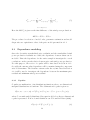
Keywords: wind power, power prices, copula, extreme value copula
2
1
Introduction
The European energy supply is increasingly dependent on renewable energy
sources. In 2012 around 23.5 percent of the European Union’s gross electricity consumption originated from renewable energy sources, however, with the
European Union’s aim of a 50 percent share of renewable energy in the total
energy consumption by 2050, an extensive transformation of the electricity
production is required. Wind energy is expected to play a major role in the
future power generation but integrating wind power into the electricity system is not without challenges. One aspect is the fact that the wind power
generation capacity depends on an uncontrollable input; the wind. This is
in clear contrast with classic fossil fuel based electricity production methods.
Wind power generation has low marginal cost, thus electricity market prices
are expected to decrease as wind power replaces power generated from gas and
coal, which has relatively high marginal production costs. However, as the
wind power production is fluctuating with the energy level of the wind, times
of no wind are expected to lead to increased market prices and enhance the
risk of price spikes. High volatility and frequent occurrences of extremely high
prices result in higher market risk and can lead to increased cost of financial
risk management.
This thesis should be seen as a contribution to the debate about wind
power as causing instability in electricity market. The dependency between
wind power production and the electricity prices in the Danish power market,
in which wind power contributes to more than 30 percent of the total electricity consumption, is investigated both in term of the general relation and
in connection to maximum prices. Overall the following questions are to be
adressed for the Danish day-ahead electricity market:
• Is the electricity price and the magnitude of the wind power production
related and if yes, in which way?
• Does unusual low wind power in-feed to the electricity system increase
the risk of extremely high prices? What could be the explanatory factors
for this result?
Inferences on the relation between the wind power in the electricity system
3
and the prices will be based on extreme value and copula theory. The research
conducted in order to answer the questions above is divided into four steps:
1. Filtering electricity prices in order to remove predictable weekly effects
as well as general trends.
2. Filtering wind power production in order to remove predictable effects
and autocorrelation from observations.
3. Investigating the general dependence structure of the full sample of filtered observations using copulas.
4. Investigating the dependence between the maximum daily prices and
minimum daily wind power production in the filtered sample using extreme value copulas.
1.1
Previous studies
Several researches point at relationship between the share of wind power and
prices. The findings of Lindström and Regland (2012) indicate that markets
with high share of renewable energy have higher probability of having spikes.
Ketterer (2014) shows that increased wind power in the German electricity
system overall reduces electricity price level but increase its volatility. Studying the impact of photovoltaic and wind energy on prices of power traded
at the European Power Exchange, Paraschiv et al (2014) likewise conclude
that renewable energy reduces the spot electricity prices. Both Ketterer and
Paraschiv et al assume linear relation between price level (and volatility) and
wind power in-feed. If price volatility increases with the share of wind power in
the power system, larger price spikes would be expected in markets with large
wind power generation. Some researches relate the market volatility, price
level, and spike probability to the share of renewable energy in the power system by comparing power markets of different regions, however, inference made
by comparing markets may be disturbed by fundamentally different market
conditions, which cannot be accounted for in the models. The approach presented in this thesis aims at relating the price spikes directly to the daily wind
power production inside the given market without assuming linear dependence.
4
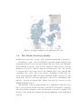
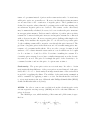
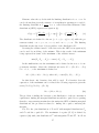
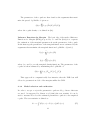
Figure 1: Danish transmission net (Energinet.dk, n.d.)
1.2
The Nordic electricity market
In this section the basic concepts of the electricity market will be presented.
Denmark is a part of the Nordic/Baltic electricity market which besides
Denmark includes Norway, Sweden, Finland, Estonia, Latvia and Lithuania.
The transmission systems of the Nordic countries are interconnected and the
Danish power grid is connected with the Swedish grid to the east and the
Norwegian grid to the north, but also the German grid to the south (Ea Energianalyse A/S, 2005). The power system of Denmark is divided into two
areas, West Denmark (DK1) and East Denmark (DK2) separated by The
Great Belt. The two areas were physically connected by a transmission line
put into operation in August 2010. Figure 1 provides an overview over the
Danish transmission net.
The structure of the electricity market can be summarized with the following: Power producers sell the electricity on the whole sale market to suppliers,
who then sell the electricity on the retail market to the final consumer. The
delivery of the electricity is ensured through the transmission and distribution
network.
5
The Nordic electricity markets has been greatly liberalized during the last
two decades opening both electricity trading and production to competition.
Liberalization introduced competition in the whole sale as well as the retail
market. While the retail market liberalization for instance gave Danish consumers the right to freely chose their power supplier, the whole sale market
liberalization has given way for the opening of the common Nordic power exchange, Nord Pool Spot, in which producers and suppliers trade power (NordReg, 2014).
Nord Pool Spot (former Nord Pool) was established as a part of the Nordic
market integration and is based in Oslo, Norway. It is owned by the national
transmission system operators, Statnett SF (Norway), Svenska Kraftnät (Sweden), Fingrid Oyj (Finland), Energinet.dk (Denmark), Elering (Estonia), Litgrid (Lithuania) and Augstprieguma tikls (Latvia) and has a market share of
84% of the total power consumption in the Nordic/Baltic market as of ultimo
2013 (Nord Pool Spot, 2013).
1.2.1
Wholesale power market
This thesis will focus on the wholesale market and in the following the concepts
necessary for understanding the wholesale market will be introduced. Wholesale market is the place where power producers and suppliers trade power and
it is said to consist of four phases or submarkets:
• Day-ahead market
• Intraday market
• Balancing market
• Forward market
The day-ahead market includes the power traded between suppliers and producers for covering the power production and consumption the following day.
The day-ahead power prices are usually referred to as spot prices and the power
to be consumed in the Nordic/Baltic region including Denmark is traded under
the name Elspot on the Nord Pool Spot exchange. The Nordic region consist of
several bidding areas, in Denmark DK1 and DK2, and for each area and each
hour a price is set on the market. The Elspot area price is determined by the
6
equilibrium between the aggregated supply and demand curves for each of the
bidding areas and hour with respect to the transmission capacity between each
area. As a reference price for the Nordic region the system price is also calculated from the sale and purchase bids disregarding the available transmission
capacity between the bidding areas. The system price is used for trading and
clearing of financial contracts, and the area prices differ from the system price
only in case of the electrical congestion due to limited transmission capacity
between the bidding areas.
Nord Pool Spot opens for intraday trading two hours after the closure of the
day-ahead market and the trading continues until one hour before delivery. The
intraday system, Elbas, gives market agents the opportunity to reach balance
between the purchased quantities and expected delivered quantities. Intraday
balancing is needed in case the day-ahead trades did not reach the agent’s
desired trade quantities or unpredicted incidents occur, e.g. an offshore wind
power plant produces less electricity than predicted. Elbas covers the Nordic
and the Baltic region as well as Germany and prices are set on a first-come
first-served principle (Nord Pool Spot, n.d.).
The balancing market, or day-after marked, is the result of deviations between planned produced/consumed power and the actual production/consumption
of power at the delivery time, causing imbalances in the electricity system. In
order to keep the system balanced at all times the system responsible operator
buy up and down regulating power. The following day accounts are settled
between the system responsible and suppliers/producers who caused the imbalances. Prices are determined according to a specific pricing model for the
balancing power administrated by the system responsible.
The forward market is the market for financial contracts used by producers
and suppliers for risk management purposes. The contracts are traded at
the NASDAQ OMX commodities exchange and includes futures, forwards and
options using the system price as reference. Moreover, Contracts for Difference,
based on the difference between area prices and system price, are traded.
In this thesis only the prices in the day-ahead market will be considered
and in the following ’price’ will refer to day-ahead price (Elspot). Moreover,
the prices are given as the daily price which is calculated by Nord Pool Spot
as the daily average.
7
2
Method
This chapter introduces the research structure as well as the employed methods. The modeling consists of four parts: First the electricity prices are filtered
in order to remove seasonality, weekly variations and other general trends in
the prices. The methods used for this purpose are presented in Section 2.1.
Also a filter for the wind power production is applied as presented in Section
2.2. After modeling prices and wind power production the dependence structure is investigated with the help of copulas. First the general dependence is
examined using the copulas presented in 2.3.1 and finally the extreme value
theory will help investigating the dependence structure of extreme events. The
extreme value approach is presented in 2.3.2.
The structure of the research is inspired by the article Aloui et al (2014),
which separates the investigation of dependence structure prices into first modeling the time series and secondly fitting copulas to the filtered series.
2.1
Price model
The electricity prices vary over the day, week and year due to the varying demand of electricity. In order to make conclusions on the relationship between
the price and the wind power production it is necessary to remove predictable
time varying effects, in other words create a series of independent, identically
distributed (IID) price residuals as the result of filtering the prices. Due to the
fairly complicated structure of the electricity prices including mean reversion,
seasonality, spikes and volatility clustering, it is not easy to find an appropriate
model for the electricity price to be used as filter. However, academic literature offers many suggestions such as hidden markov chain models, state-space
models and models using external regressors.
In this section the model used in this thesis will be presented, and reasons
behind the model will be explained. The notation regarding the model is used
as in Cryer and Chan (2008) and is in the following explained.
Return measures not used Given a series of prices {Pt }, the return is det−1
and the continuously compounded return (log-return) as
fined as Rt = PtP−P
t−1
rt = log(Pt ) − log(Pt−1 ). In classic financial modeling it is common to use re8
turns or log-returns instead of prices as the return series tend to be stationary
while price series are generally not. However, in this thesis return measures
are not used due to the occurrences of negative prices. The logarithm is not
defined for negative values, thus the log-return series would have missing values whenever negative prices are observed. The return, on the other hand,
may be numerically calculated, however, it does not reflect the price structure
in an appropriate manner. Under normal conditions of positive prices positive
returns are connected with price increase and negative returns are connected
with a decrease in price. However, negative prices challenge this simple relationship. If for instance the negative price P t−1 is followed by a positive price
P t the resulting return will be negative even though the price increased. The
problem of negative prices is the main reason for not transforming prices into
returns or log-returns in this thesis. Moreover, the concept of return is well
understood for classic financial assets such as a stock which can be bought
for Pt−1 at time t − 1 and be sold for Pt at time t resulting in a return. For
electricity prices return does not have a similar interpretation as the electricity cannot be stored. The price Pt is simply the price of the electricity to be
consumed at time t and not the price of a given asset at time t.
Stationarity The power price series are not stationary. In order to obtain
stationarity the first difference of the power prices are used instead of the price
itself, ∆Pt = Pt −Pt−1 . Stationarity is an important feature of the series and it
is needed for applying the filters. The validity of the stationarity assumption
will be examined by applying a unit root test. In this thesis the test used
to reject stationarity is the test of Kwiatkowski-Phillips-Schmidt-Shin (KPSS)
defined in Kwiatkowski et al (1992).
ARMA In order to remove autocorrelation from the electricity price series
an autoregressive moving average (ARMA) model for the first difference of
prices is chosen.
The ARMA process, which includes p AR terms and q MA terms, is specified as
∆Pt = et +
p
X
φi ∆Pt−i +
i=1
q
X
j=1
9
θj et−j
(1)
Above ∆Pt is the first difference of the price at time t and et is the stochastic
error term at time t. The parameters φi and θj relate to the AR and MA part
of the model, respectively, and the model is referred to as ARMA(p,q).
Weekday indicator variables While a lot of electricity is consumed during
the weekdays, the electricity consumption is low during the weekend. Due to
this pattern in consumption, the electricity prices follow a weekly pattern of
low prices in the weekend and high prices during the weekdays. In order to
remove weekly effects from the resulting residuals, weekday indicator variables
are added to the ARMA(p,q) model.
∆Pt = et +
p
X
φi ∆Pt−i +
i=1
q
X
θj et−j +
j=1
7
X
ζk I{t∈Wk }
(2)
k=1


1
if t ∈ Wk
I{t∈Wk } = 
0 otherwise
I{t∈Wk } is the indicator variable activating the parameter ζk when the day t
falls on the kth day of the week. The model presented in equation (2) will in
the following be referred to as the mean equation.
GARCH While the mean equation aims at filtering away autocorrelation i
price series, the volatility clustering of the prices also needs to be taken into
account in the model. The price volatility depends on the general market
conditions and may vary over time, which means that some periods have low
volatility while others may have high. The implication of conditional volatility
is that the errors {et } may not be identically distributed.
Volatility clustering (heteroscedasticity) can be modeled using a generalized autoregressive conditional heteroscedasticity model (GARCH). With the
GARCH model variance is modeled as conditional on previous observations.
The GARCH(P,Q) model is presented in equation (3) below:
2
σt|t−1
=ω+
P
X
2
βi σt−i|t−(1+i)
i=1
+
Q
X
j=1
et = σt|t−1 εt
10
αj e2t−j
(3)
By taking the changing volatility into consideration the resulting standardized residuals {εt } can be considered IID and be used for modeling the
dependence structure with wind power production.
Estimation method The model parameters to be estimated are φi for i =
{1, 2, ..., p}, θj for j = {1, 2, ..., q}, ζk for k = {1, 2, ..., 7}, βi for i = {1, 2, ..., P }
and αi for i = {1, 2, ..., Q}.
The parameters of the ARMA-GARCH model can be found as the arguments to the maximum log-likelihood (ML). The maximum likelihood of
ARMA-GARCH models can be computed using a state-space formulation and
a Kalman filter to recursively generate prediction errors and their variances
and then use the prediction error decomposition of the likelihood function. The
detailed description of the method can be found in Cryer and Chan (2008).
The log-likelihood is calculated using a prespecified residual distribution.
The assumption of distribution is determined experimentally as the one fitting
the residuals more accurately. In this thesis the choice of residual distribution
is between normal and student-t distribution.
2.1.1
Model selection
Akaike information criteria The models for electricity prices and wind
power production will be selected according to the Akaike’s Information Criterion (AIC). The criterion states that the preferred model is the one that
minimizes:
AIC = −2l + 2k
where l is the maximum log-likelihood and k is the number of parameters in
the model. While the likelihood increases with the number of parameters in
the model, the AIC helps to avoid selecting a model with too many parameters
thus ensures selection of a parsimonious model.
Autocorrelation The goal of fitting models to the price as well as the wind
power time series is to filter out IID residuals, which includes residuals being
free of autocorrelation.
The autocorrelation of the price series is investigated using the sample
autocorrelation function (ACF). Significant autocorrelation indicates the need
11
of filtering data with an ARMA model. After fitting the ARMA-GARCH
model the standardized residuals are checked for autocorrelation with visual
inspection and with the application of the Weighted Ljung-Box test to the
residuals.
The magnitude of the autocorrelation on individual lags can be inspected by
looking at the sample autocorrelation function (ACF) of the residuals. Values
of the sample functions departing greatly from zero indicate autocorrelation
at the given lag, and may lead to rejection of the model for not successfully
resulting in autocorrelation free residuals. The limits for significance at a
√
95% level is set as ±λ0.975 / n where n is the sample size and λ0,975 is the
97,5% upper quantile of the standard normal distribution. Hence the estimated
√
ACF values at individual lags has to be greater than λ0.975 / n or smaller
√
than −λ0.975 / n in order to be considered significantly different from zero.
Moreover, in order to take into account the autocorrelation magnitudes as
group the Weighted Ljung-Box test suggested by Fisher and Gallagher (2012)
is applied.
In the Weighted Ljung-Box test applied to residuals from an ARMA(p,q)
model the test statistic is given as:
Q = n(n + 2)
K
X
k=1
wk
ρˆ2k
n−k
!
where n is the sample size, and the estimated autocorrelation of lag k, ρˆk , and
the weight w(k) are given with the following equations:
ρˆk =
X
1 n−|k|
(εt+|k| − ε)(εt − ε)
n i=1
K −k+1
K
Under the null hypothesis that the residuals have no autocorrelation up to lag
K, the distribution of the test statistics Q can be approximated with a gamma
distribution, for which the shape and scale parameters are given as:
wk =
α=
3
K(K + 1)2
4 2K 2 + 3K + 1 − 6K(p + q)
12
β=
2 2K 2 + 3K + 1 − 6K(p + q)
3
K(K + 1)
For values of Q < Γ0.95 (α, β) the residuals show no significant autocorrelation
and the model can be accepted.
Homoscedasticity The residuals can be checked for remaining heteroscedastic effects by investigating the squared standardized residuals. In case the
residuals exhibit heteroscedasticity the squared residuals will show autocorrelation. The sample ACF of the squared residuals is useful for identifying autocorrelation at individual lags, and with a Ljung-Box test applied to squared
standardized residuals the hypothesis of homoscedasticity can be tested. The
test statistics is given as
K
X
Q∗ = n(n + 2)
k=1
ρˆ2k
n−k
!
where ρˆ2k is the estimated k-lag autocorrelation of the squared residuals. Q∗ is
χ2 distributed with K degrees of freedom under the null hypothesis, implying
that the null hypothesis of homoscedasticity is rejected on a 5% confidence
level if Q∗ > χ20.95 (K).
2.2
Wind power model
The wind power production depends on the weather conditions. During periods with little wind the generation is low compared to periods with high
wind speeds, and since the weather conditions one day is highly related to the
weather the previous days, so is the wind power production. Like the electricity prices the wind power production series also exhibits heteroscedasticity.
Due to autocorrelation and heteroscedasticity the wind power production is
also modeled as an ARMA-GARCH process with the model specifications as
below:
∆W Pt = et +
p
X
φi ∆W Pt−i +
i=1
q
X
j=1
13
θj et−j
(4)
2
σt|t−1
=ω+
P
X
2
βi σt−i|t−(1+i)
i=1
+
Q
X
αj e2t−j
(5)
j=1
et = σt|t−1 εt
Here the ∆W Pt is given as the first difference of the wind power production:
∆W Pt = W Pt − W Pt−1
The procedure for selection of model order, parameter estimation and model
diagnostics are equivalent to that of the price model presented in 2.1.1.
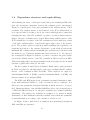
2.3
Dependence modeling
Once the electricity standardized price residuals and the standardized wind
power production residuals are found, the dependence between them can be
modeled. First the dependence for the entire sample is investigated to reach
conclusions on the general relation between price and wind power production.
For this purpose, the notion of copulas will be introduced in Section 2.3.1.
Secondly the extreme value dependence will be examined using the component
wise block maxima. The bivariate extreme value theory introduced in Section
2.3.2 will be used to investigate the dependence between the maximum price
residual and minimum wind power residual.
2.3.1
Copulas
Copulas are multivariate joint distributions functions whose one-dimensional
marginal distributions are uniform. The d-dimensional copula is given as
C(u1 , u2 , ..., ud−1 , ud ) = P (U1 ≤ u1 , U2 ≤ u2 , ..., Ud−1 ≤ ud−1 , Ud ≤ ud )
where U i are uniform(0,1) distributed. In equation (6) below, the two-dimensional
copula is presented. A more formal definition can be found in Nelsen (2004).
C(u, v) = P (U ≤ u, V ≤ v)
14
(6)
The most important characteristics of the two-dimensional copula are:
C(u, 1) = u, C(1, v) = v
C(u, 0) = 0 = C(0, v)
W (u, v) ≤ C(u, v) ≤ M (u, v)
where W (u, v) = max(u + v − 1, 0) and M (u, v) = min(u, v). The inequality
above is called Fréchet-Hoeffding bounds inequality.
In case of independence between the variables the formulation can be reduced to the independence copula:
C(u, v) = uv
(7)
By applying Sklar’s theorem the theory of copulas becomes useful for modeling dependence structures between random variables. For the 2-dimensional,
continuous case Sklar’s theorem can be expressed as:
Let F be a joint distribution function with margins FX and FY .
Then there exists a copula C such that for all x, y in R,
F (x, y) = C(FX (x), FY (y))
(8)
If FX and FY are continuous then C is unique. If C is a copula and
FX and FY are distribution functions, then the function F defined
by (8) is a joint distribution function with margins FX and FY .
(Nelsen, 2004)
According to Sklar’s theorem the copula contains all information about the dependence structure, and the task of modeling the joint distribution of random
variables can be reduced to finding the marginal distributions FX and FY and
the copula C.
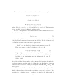
In this thesis the Normal, Gumbel, Clayton, Frank and t copula will be
fitted to the residuals such that the best fitting copula can be selected. The
specifications of the five types of copulas to be fitted to the full sample of
15
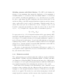
Copulas
Name
Normal
C(u, v)
Φρ (Φ (u), Φ← (v))
←
Gumbel
θ
θ
exp − (−logu) + (−logv)
1/θ Parameter
−1 ≤ ρ ≤ 1
Independence
ρ=0
1≤θ<∞
θ=1
−1 < θ < ∞, θ 6= 0
θ→0
Frank
−θ
−1/θ
(max(u
+ u−θ
2 − 1, 0))
1
−θu
−θv
(e −1)(e −1)
1
− θ log 1 +
e−θ −1
−∞ < θ < ∞, θ 6= 0
θ→0
t
←
tν,ρ (t←
ν (u), tν (v))
ν > 0, −1 ≤ ρ ≤ 1
ρ = 0, ν → ∞,
Clayton
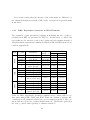
Table 1: List of bivariate copulas used for modeling the dependence. The table
gives both the parametric description of the copula, the permitted values of
the parameters and the parameter values leading to independence. Φ← is the
inverse cumulative distribution function of the normal distribution, Φρ is the
bivariate normal distribution with linear covariance parameter ρ. t←
ν is the
inverse cumulative distribution function of the t-distribution with ν degrees of
freedom, while tν,ρ is the bivariate cumulative t-distribution.
residuals are presented Table 1.
Note that the price residuals are denoted {Xt } and its corresponding uniform transform {ut }, while the wind power residuals are named {Yt } with its
the uniform transform {vt }.
2.3.2
Extreme value copulas
The aim of the thesis is to investigate the extreme value dependence between
the electricity prices and the wind power production. Extreme value theory
introduces the framework for modeling the maximum or minimum of variables
using the limiting extreme value distribution. The general ideas of the extreme
value theory are presented below.
First the univariate case is considered as described in Coles (2001). For a
series of IID stochastic variables, X1 , X2 , ..., Xn with the common distribution
FX the maximum Mn is defined as:
Mn = max(X1 , X2 , ..., Xn )
The distribution of Mn can then be expressed in terms of FX :
P (Mn ≤ z) = P (X1 ≤ z, X2 ≤ z, ..., Xn ≤ z) =
n
Y
i=1
16
P (Xi ≤ z) = FXn (z)
Extreme value theory deals with the limiting distribution for n → ∞. It
can be shown that given the existence of normalization parameters an and bn ,
n
the limiting distribution of Mna−b
is a so called Generalized Extreme Value
n
distribution (GEV) expressed in equation (9).
!
G(z) = P
z−µ
Mn − bn
≤ z = exp − 1 + γ
an
σ
− 1 !
γ
(9)
The distribution is defined for the set {z : 1 + γ(z − µ)/σ > 0} while the parameters satisfy −∞ < µ < ∞, σ > 0, and −∞ < γ < ∞. The limiting
distribution takes the form of (9) regardless of the distribution FX .
By using the additive inverse of the data series the GEV as in equation (9)
can be used for modeling of the minima. This is the result of the minimum
being expressed in terms of the maximum of the additive inverse:
min(X1 , X2 , ..., Xn ) = −max(−X1 , −X2 , ..., −Xn )
In the multivariate case the maximum can be defined as the vector of componentwise maxima. Given the d-dimensional series Xi = (Xi1 , Xi2 , ..., Xid )
for i = 1, 2, ..., n the maximum is defined as:
Mn = (Mn,1 , Mn,2 ..., Mn,d ), where Mn,j = max(X1j , X2j , ..., Xnj )
In this thesis only bivariate data will be used. For bivariate data the
expression of the maximum can be reduced the following expression given the
series (X1 , Y1 ), (X2 , Y2 )..., (Xn , Yn ).
Mn = (Mn,X , Mn,Y )
(10)
The problem of finding the bivariate joint distribution of the two maxima is
equivalent to finding the marginal distributions and the copula. By recognizing
that the componentwise maxima have the univariate GEV as limiting marginal
distributions, the problem is reduced to finding the copula connecting the
margins.
Let F be the joint distribution of X and Y with marginal distributions FX
and FY and the copula CF . The maximum of n pairs (X, Y ) is defined by
equation (10) with joint distribution F n and marginals FXn and FYn . It follows
17
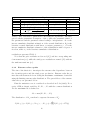
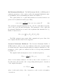
Extreme value copulas
C(u, v)
Name
Gumbel
exp − (−logu)θ + (−logv)θ
Tawn
uvexp −θ logu·logv
log(uv)
Galambos
uvexp
Husler-Reiss
1/θ (−logu)−θ + (−logv)−θ
exp loguΦ
logvΦ
1
θ
+ 21 θlog
1
θ
+ 21 θlog
−1/θ Parameter
Independence
1≤θ<∞
θ=1
0≤θ≤1
θ=0
0<θ<∞
θ→0
0<θ<∞
θ→0
−logu
+
−logv −logv
−logu
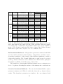
Table 2: List of extreme value copulas used for investigating the extreme
dependence. Φ denotes the cumulative standard normal distribution function.
that the copula Cn of Mn is given by
1
1
Cn (u, v) = CF (u n , v n )n
If there exist a C F such that the copula Cn → C for n → ∞, then C is called
an extreme value copula. Moreover, it can be shown that the bivariate copula
C is an extreme value copula if and only if
C(u, v) = (u · v)A(log(u)/log(u·v)) , (u, v)(0, 1]2 / {(1, 1)}
(11)
where A : [0, 1] → [ 21 , 1] is convex and satisfies max(t, (1 − t)) ≤ A(t) ≤ 1 for
all t[0, 1] (Gudendorf and Segers, 2009).
The function A(t) is called Pickands dependence function and is useful for
understanding the dependence structure. The upper bound A(t) = 1 gives the
independence C(u, v) = u · v while the lower bound A(t) = max(t, (1 − t))
corresponds to perfect dependence resulting in the copula C(u, v) = min(u, v).
Pickands dependence function can also be used to calculate the upper tail
dependence by:
χ = limu→1 P (U > u|V > u) = 2(1 − A(1/2))
(12)
In this thesis four different types of EV copulas will be used for modeling
the extreme value dependence and the four kinds is presented in Table 2.
18
Modeling extremes with Block Maxima The GEV is the limiting distribution of the maximum, that means the distribution of the maximum of
an infinite number of observations. Even if an infinite number of observations
were available, modeling the distribution of one observations is not possible.
In order to approximate the GEV distribution the data is divided into blocks,
and the modeling of the GEV marginal distribution functions and the extreme
value copulas will be based on the block maxima. With this method the bivariate data series {Xi , Yi } is divided into blocks of length l, and for each
block the component wise maxima are found. In other words, for the blocks
i {1, 2, ..., N } of length l the component wise block maxima is given by:
i
i
Mli = (Ml,X
, Ml,Y
)
(13)
For appropriate choice of block length the maxima will be approximately GEV
n
o
n
o
i
i
distributed, thus GEV distributions are fitted to the series Ml,X
and Ml,Y
.
According to Coles (2001) selecting a block length is ultimately a question of
trade-off between bias and variance: Long blocks will result in few observations
resulting in large variance of the parameter estimates while short block lengths
will give more observations but not from the GEV distribution as the GEV by
definition is the limit distribution of Mn for n → ∞.
The series of component wise block maxima {Mli } may not consist of observed pairs from the original series, however, it is still useful for inferences on
the joint extreme value behavior.
2.3.3
Estimation method
The copula parameters are estimated using three difference methods, Full Maximum Likelihood (FML), Canonical Maximum Likelihood (CML), and Inference Functions for Margins (IFM). The first and the latter give a full parametric description of both copula and marginal functions while the CML method
uses empirical marginals when estimating the parameters of the copula.
Each method has advantages and disadvantages, and consistency across
parameter values resulting from the different methods indicates reasonable
assumption of the marginal distribution functions. With this reason all three
methods are applied. The methods are used when investigating both the full
sample dependence structure and the extreme value dependence structure.
19
Full Maximum Likelihood The Full Maximum Likelihood (FML) method
estimates parameters of the copula as well as the marginal distribution functions simultaneously by maximizing the full model’s likelihood.
The copula density for a copula with parameters θ is in the bivariate case
given as below (Gudendorf and Segers, 2009):
∂2
Cθ (uX , uY ), (uX , uY )(0, 1)2
cθ (uX , uY ) =
∂uX ∂uY
(14)
The parametric marginal distributions FX,ϕ and FY,% with unknown parameters ϕ and % give the uniform margins. The parameters of the copula and
the marginal distributions is found as the arguments that maximize the loglikelihood stated below,
l(θ, ϕ, %) =
n
X
logcθ (FX,ϕ (Xi ), FY,% (Yi ))
i=1
The FML estimation may require high computational power, thus other
less computer intensive methods are suggested.
Canonical Maximum Likelihood The Canonical Maximum Likelihood
(CML) method consist of a two step estimation where the observations first
are transformed into uniform margins using the empirical distributions. The
parameters of the copula are estimated in the second step using maximum
log-likelihood.
The empirical uniform margins are based on rank and given by:
Fˆ (x) =
n
1 X
I (Xi ≤ x)
n + 1 i=1
(15)
where I is the indicator function. In other words, for the observation xt of
the time series {Xi } at time t the corresponding uniform pseudo-observation
of the empirical margin is:
uˆt = Fˆ (xt ) =
i
n+1
(16)
where i is the rank (order) of the observation xt and n is the total number
observations.
20
The parameters of the copula are then found as the arguments that maximize the pseudo log-likelihood given as:
l(θ) =
n
X
logcθ (FˆX (Xi ), FˆY (Yi ))
i=1
where the copula density cθ is defined in (14).
Inference Functions for Margins The basic idea of the method Inference
Functions for Margins (IFM) proposed by Joe and Xu (1996) is to separate
the estimation of the marginal parameters from the parameters of the copula.
In the first step the parameters of the marginal functions are estimated by the
arguments that maximize the marginal functions log-likelihood,ϕand
ˆ
%ˆ:
l(ϕ) =
n
X
logfX,ϕ (Xi )
i=1
l(%) =
n
X
logfY,% (Yi )
i=1
where fX,ϕ and fY,% are the marginal density functions. The parameters of the
copula are then estimated by maximizing the log-likelihood
l(θ) =
n
X
logcθ (FX,ϕˆ (Xi ), FY,ˆ% (Yi ))
i=1
This approach is computationally less intensive that the FML but still
allows for parametric models of the margins unlike the CML.
2.3.4
Model selection and verification
In order to accept or reject the parametric copula model goodness-of-fit tests
are used. As suggested by Genest et al (2006) the test statistic Sn can be
used to measure how close the estimated parametric copula is to the empirical
copula. The test statistics is defined as
ˆ
Sn = n
(Cn (u, v) − Cθn (u, v)) dCn (u, v)
21
(17)
where Cθn is the parametric copula and Cn is the empirical copula. Cn is given
in terms of the uniform pseudo-observations (ˆ
ui , vˆi ) as in equation (16):
Cn (u, v) =
n
1X
I(ˆ
ui ≤ u, vˆi ≤ v)
n i=1
For the extreme value copulas a goodness-of-fit test based on Pickands
dependence function can be applied. The test statistic Mn is defined as in
Genest et al (2011):
ˆ
1
|An (t) − Aθn (t)|2 dt
Mn =
(18)
0
where An (t) is the empirical Pickands function and Aθn (t) is the Pickands
function resulting from the parametric model of the copula. The empirical
Pickands function is estimated with the Capéraà-Fougeres-Genest method as
presented in Capéraà et al (1997).
The p-value associated with the test statistics can be calculated with parametric bootstrap, however, as this method is very computer intensive, the
multiplier approach presented by Kojadinovic and Yan (2010) is used for the
Sn -test.
2.3.5
Identifying independence
An important question in relation to the investigation of the dependence structure between the price and wind power is how to identify the case of independence.
Likelihood ratio test Independence can be expressed in terms of the independence copula as in equation (7), and if the independence copula is nested
within the parametric copula a likelihood ratio test can be used to reject the
hypothesis of independence. However, the likelihood ratio test requires that
the parameter values which result in the independence copula are inside the
boundaries - and not on the boundary - of the permitted parameter values. Of
the copulas presented in Table 1 and 2 only the normal copula lives up to this
condition, as the parameter value ρ = 0 leads to independence and lie within
the boundaries −1 ≤ ρ ≤ 1. Hence, only for the normal copula the likelihood
22
ratio test can be used.
The likelihood ratio test statistic is defined as
D = 2(lθˆ − l0 )
(19)
where lθˆ is the log-likelihood of the model, Mθ , with estimated parameters θˆ
and l0 is the log-likelihood of the independence copula. Under the null hypothesis that the observations are independent, the test statistic will be approximately χ2 (p)-distributed. The p degrees of freedom are equal to the difference
in number of parameters in the two models, however, as the independence
copula has no parameters p will be the number of parameters in Mθ (Coles,
2001).
Due of the limitations in the application of the likelihood ratio test a nonparametric method using visual inspection is also employed.
χ-plot and χ-plot Independence between bivariate data can be identified
using χ- and χ-plots. The plots are based on the definition of the asymptotic,
upper tail dependence as in equation (12) and idea of the χ-plot is in the
following explained as in Coles et al (1999). The upper tail dependence is
given as:
χ = limu→1 P (U > u|V > u)
f or u → 1 and C(u, u) =
Observing that P (U > u|V > u) → 2 − log(C(u,u))
logu
P r(U < u, V < u), the chi-function χ(u) is be defined as:
χ(u) = 2 −
log(P r(U < u, V < u))
, 0<u<1
logu
(20)
By this definition of the χ-functions the upper tail dependence is given as:
χ = limu→1 (χ(u))
For independent variables (U, V ) the χ(u) is 0 for any permitted value of u. If
(U, V ) are upper tail independent χ(u) → 0 for u → 0 . Plotting χ(u) against
u gives the basis for determining overall lack of dependence and in the data.
In case the data is dependent but asymptotic independent χ(u) may con23
verge very slowly towards zero for u → 1, resulting in χ(u) being significantly
greater than zero even for u-values close to one. This makes it difficult to
identify the upper tail independence, thus a new dependency measure, χ, is
introduced.
Denoting the survivor function P r(X > x, Y > y) by F¯ (x, y) the copula,
C¯ can be defined as:
¯ X (x), FY (y))
F¯ (x, y) = 1 − FX (x) − FY (y) − F (x, y) = C(F
where
¯ v) = 1 − u − v − C(u, v)
C(u,
Similarly to the definition of χ(u) in equation (20), χ(u)
¯
can be defined as:
χ(u)
¯
=
2log(1 − u)
2log(P r(U > u))
−1=
¯ u) − 1, f or 0 < u < 1
log(P r(U > u, V > u))
logC(u,
and
χ¯ = limu→1 χ(u)
¯
With this definition χ(u)
¯
lies between -1 and 1, and asymptotic dependence
¯ v) = (1 − u)(1 − v) so that
results in χ¯ = 1. For independent variables C(u,
χ(u)
¯
= 0 for all u[0, 1]. By plotting χ(u)
¯
against u, the dependence can
be inspected. It can be proved that for Normal copula the χ¯ is equal to the
dependence parameter ρ and the convergence towards ρ is approximately linear
for u > 0.5. This makes the inspection of the tail dependence easier in the
χ-plot
¯
compared with the χ-plot.
24
3
3.1
Analysis and results
Data
The data used in this thesis consist of 1080 observations of the daily day-ahead
electricity prices and the daily wind power produced in the two areas, DK1
and DK2, for the period from 1 January, 2012 to 15 December, 2014. Prices
are given as daily average in Danish Krone (DKK) and the daily wind power is
the aggregated hourly production measured in MWh. Both series are publicly
available on the website of Nord Pool Spot.
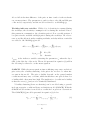
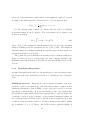
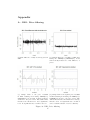
3.2
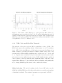
Daily prices
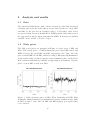
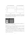
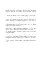
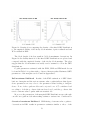
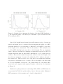
The daily power prices are presented in Figure 2 for the areas of DK1 and
DK2. The average price of 1 MWh during the period was DKK 264.47 and
DKK 272.21 for the areas DK1 and DK2, respectively. On 7 June, 2013, the
price reached DKK 3253 in DK1, which according to Energinet.dk (Rasmussen,
2013) was the result of reduced capacity on the transmission line over the Great
Belt combined with limited possibility for importing from Germany. Negative
prices occur in DK1 as well as in DK2.
Figure 2: Daily electricity prices in DK1 (West Denmark) and DK2 (East
Denmark). Limited interregional transmission capacity resulted in price spike
in DK1 on June 7, 2013. In both DK1 and DK2 negative power prices have
been observed.
25
In this section the results of the ARMA-GARCH modeling of the prices are
presented. The choice of the model will be further justified and the goodnessof-fit of the models will be discussed.
While there is no clear sign of yearly seasonality during the 35.5 months of
observations, the prices do show a weekly periodicity, which supports the idea
of including weekly periodicity in the model. Moreover, the price series do
not look stationary suggesting that modeling the first difference of the power
prices is appropriate.
3.2.1
DK1: Price model in West Denmark
The KPSS test for the first difference of price series indicates that the assumption of stationarity cannot be rejected at a 95% confidence level.
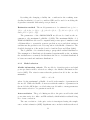
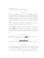
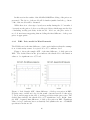
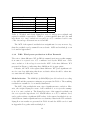
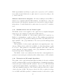
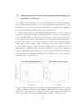
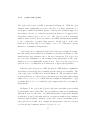
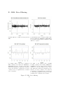
Figure 3 shows the sample ACF of the first difference of daily prices in
DK1. The dashed lines in the plots indicate the threshold for the function
values to be significant at a 95% level.
Figure 3: Left: Sample ACF of first difference of daily power prices in DK1.
Negative autocorrelation for lag 1 is the result of mean reversion. Peaks at lag
7, 14, 21 and 28 support the idea of weekly periodicity in the price series. The
dashed lines indicate the threshold for 95% significance level. Right: Sample ACF of squared first difference of daily power prices in DK1. Significant
value for lag 1 indicates heteroscedasticity and justifies the use of GARCH
specification in the model.
26
As expected for mean-reverting processes the autocorrelation with lag 1 of
the first difference series is negative. Mean-reversion secures that the prices
return to the mean level, which implies that large prices tend to be followed
by lower prices and low prices tend to be followed by higher. A clear weekly
periodicity exists, expressed as ACF peaks for lags that are a multiples of
seven. This support the choice of using the weekday indicators in the model.
The ACF of the squared first difference of daily prices also presented in
Figure 3, are significant for lag 1, thus volatility clustering should be taken
into account in the model. This is done through modeling the conditional
variance within the GARCH framework.
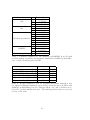
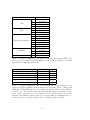
Model order selection According to the AIC, the ARMA(3,3)-GARCH(1,1)
model with weekday indicators and student-t distributed residuals is selected
and its estimated parameter values are presented in Table 3.
The sample ACF of the residuals shows no significant values, which indicates that all autocorrelation in the price series has successfully been filtered
away with the selected model. In particular, the weekly periodicity has been
been removed as no clear autocorrelation on lags that are multiples of seven exists. The test results of the Ljung-Box tests are presented in Table 4. Weighed
Ljung-Box tests for the residuals result in high p-values thus support that no
further autocorrelation can be detected.
Moreover, the sample ACF of the squared residuals is not significantly different from zero for any non-zero lags. Together with the test results of the
Ljung-Box test for squared residuals, in which null hypothesis of no autocorrelation can be rejected for p-values smaller than 0.05, it can be concluded that
there exist no further significant heteroscedastic effects. ACFs and residual
plot can be found in Appendix A.
27
Parameter
AR
MA
Weekday parameters
GARCH
t-dist shape parameter
φ1
φ2
φ3
θ1
θ2
θ3
ζ1
ζ2
ζ3
ζ4
ζ5
ζ6
ζ7
ω
α
β
ν
Estimated value
1.835061
-1.357896
0.4471407
-2.136831
1.614041
-0.4704461
53.81275
6.287118
3.096599
-4.074114
-9.863092
-29.92216
-18.68064
1115.457
0.3651083
0.2925828
3.662627
Table 3: Parameter estimates for the ARMA(3,3)-GARCH(1,1) model with
weekday indicator variables and student-t distributed residuals for first difference of daily electricity prices in DK1.
Ljung-Box test
Residuals (lag = 20, weighed)
Residuals (lag = 30, weighed)
Residuals (lag = 50, weighed)
Squared residuals (lag = 12)
Squared residuals (lag = 20)
Squared residuals (lag = 30)
Test statistic
6.4077
10.0118
14.9243
0.4522
0.4809
0.5556
p-value
0.9989
0.9792
0.9952
1
1
1
Table 4: Weighed Ljung-Box test for residuals and classic Ljung-Box test
for squared residuals resulting from modeling electricity prices in DK1 with
ARMA(3,3)-GARCH(1,1) model. Null hypothesis of no autocorrelation is rejected for p-values smaller than 0.05. The null hypothesis cannot be rejected
for any of the tests.
28
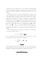
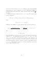
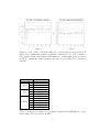
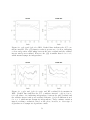
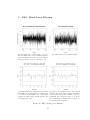
Figure 4: Left: ACF of first difference of power prices in DK2. There exist significant autocorrelation for lag 7, 14, 21 and 28 indicating the need of
adding weekday indicator variables in the model. Right: ACF of squared first
difference power prices in DK2. The dashed line indicates the threshold value
for significance at a 95% confidence level.
3.2.2
DK2: Price model for East Denmark
The analysis of the price series in DK2 is equivalent to that of DK1. The
KPSS test cannot reject null hypothesis of stationarity on a 95% confidence
level. ACF of the first difference of daily prices is presented in Figure 4, in
which evidence for weekly periodicity is found in terms of the clear 7 day
pattern in the ACF including significant autocorrelation at lag 7, 14, 21 and
so on. Negative autocorrelation for lag 1 is the result of mean reversion in the
price series, however, unlike the price series of DK1 significant autocorrelation
can be found for other lags than the first. Significant values of the ACF of the
squared first difference of prices indicate heteroscedasticity and justifies the
need of using GARCH specifications for the conditional variance.
Model selection The model resulting in the lowest AIC value was the
ARMA(4,3)-GARCH(1,1) model with weekday indicator variables and studentt distributed residuals. The estimated parameters are presented in Table 5.
29
Parameter
AR
MA
Weekday parameters
GARCH
t-dist shape parameter
φ1
φ2
φ3
φ4
θ1
θ2
θ3
ζ1
ζ2
ζ3
ζ4
ζ5
ζ6
ζ7
ω
α
β
ν
Estimated value
2.131264
-1.659532
0.420233
0.065418
-2.539241
2.300945
-0.763197
48.62527
13.41433
-5.269275
-3.900434
-9.363129
-30.08975
-13.55165
75.1294
0.172647
0.816063
4.266136
Table 5: Parameter estimates for the model for daily power prices in DK2. The
chosen model is ARMA(4,3)-GARCH(1,1) with weekday indicator variables
and student-t distributed residuals.
Ljung-Box test
Residuals (lag = 20, weighed)
Residuals (lag = 30, weighed)
Residuals (lag = 50, weighed)
Squared residuals (lag = 12)
Squared residuals (lag = 20)
Squared residuals (lag = 30)
Test statistic
6.0431
9.901
17.2826
2.3364
4.7286
8.1356
p-value
1
0.9913
0.9775
0.9987
0.9998
1
Table 6: Weighed Ljung-Box test for residuals and classic Ljung-Box test
squared residuals resulting from modeling the electricity prices of DK2 with
ARMA(4,3)-GARCH(1,1). In case p-values are smaller than 0.05 the null hypothesis of no autocorrelation in the residuals and squared residuals, respectively, can be rejected at a 95% confidence level. As all p-values are greater
than 0.05 the null hypothesis can not be rejected, thus no significant autocorrelation nor heteroscedastic effects can be identified in the residuals.
30
The ACF of the residuals indicates no remaining autocorrelation and this is
supported by the weighed Ljung-Box test presented in Table 6, which cannot
reject the assumption of no autocorrelation in the residuals on a 95% confidence level with all p-values greater than 0.05. Likewise the hypothesis of no
ARCH effects in the residuals can not be rejected on a 95% confidence level
by the Ljung-Box test applied to the squared residuals, and the ACF of the
squared residuals are insignificant for all non-zero lags, thus no remaining heteroscedastic effects can be identified in the residuals. ACFs and residual plots
can be found in Appendix B.
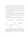
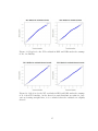
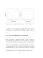
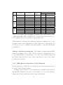
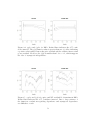
Figure 5 shows the QQ-plots for the price residuals in DK1 as well as DK2.
The theoretical quantiles of the student-t distribution are plotted against the
empirical quantiles of the residuals. The plots confirm that the assumption
of student-t distributed residuals is appropriate for both areas and only the
tails of the residual distributions seem to deviate a little from the tails of the
student-t distribution.
In conclusion, when using the estimated model as filter, the remaining price
residuals can be assumed to be independently student-t distributed.
Figure 5: QQ-plot of the price residuals of DK1 and DK2, repectively. The
assumption of student-t distributed residuals is appropriate as the empirical
quantiles plotted against the theoretical quantiles from the student-t distribution form a straight line. Only the most extreme observations deviate from
the line, indicating that the student-t tail distributions are thinner than that
of the observations.
31
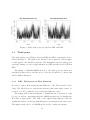
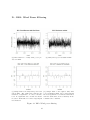
Figure 6: Daily wind power produced in DK1 and DK2.
3.3
Wind power
The daily wind power (WP) produced in DK1 and DK2, respectively, is presented in Figure 6. The wind power has the lower bound zero and an upper
bound equal to the installed capacity. The maximum observed wind power
generated during one day is approximately 80 GWh in DK1 and 25 GWh in
DK2.
The fitting of ARMA-GARCH models to the wind power production is
presented in this section, and the choice of the model and the goodness-of-fit
will be further discussed.
3.3.1
DK1: Wind power in West Denmark
In order to achieve stationarity the first difference of the WP is used for modeling. The KPSS test for stationarity indicates that stationarity cannot be
rejected on a 95% confidence level for the first difference series.
The sample ACF is shown in Figure 7. Significant autocorrelation do exist
for lag one and two suggesting that the ARMA-specification for filtering the
WP data is appropriate. The ACF of the squared first difference WP has
significant values for some lags indicating heteroscedasticity in the data series.
This supports the choice of GARCH-model for the conditional variance.
32
Figure 7: Left: ACF of the first difference of daily wind power produced in
DK1. The dashed lines indicate significance threshold for a 95% confidence
level. Significant autocorrelation is seen for lag one and two. Right: ACF of
the squared first difference of WP in DK1.
Parameter
AR
φ1
θ1
MA
θ3
ω
GARCH α
β
Estimated value
0.21306587
-0.63528845
-0.31117248
2.21408162
0.02306379
0.96517653
Table 7: Parameter estimates from the fitting ARMA(1,2)-GARCH(1,1) to
the daily wind power production in DK1.
Model selection According to the AIC the model to be selected for the WP
in DK1 is the ARMA(1,2)-GARCH(1,1) with normal distributed residuals.
The estimated parameters are presented in Table 7.
The sample ACF of the residuals shows no sign of further autocorrelation
as no ACF values are significant for any non-zero lag. Likewise, the Weighed
Ljung-Box test cannot reject the hypothesis of no autocorrelation on a 95%
confidence level, as no p-values are smaller than 0.05. The Ljung-Box test for
the squared residuals can also not reject lack of heteroscedastic effects. Test
results are presented in Table 8.
33
Ljung-Box test
Test statistic
p-value
Residuals (lag = 20, weighed)
Residuals (lag = 30, weighed)
Residuals (lag = 50, weighed)
Squared residuals (lag = 12)
Squared residuals (lag = 20)
Squared residuals (lag = 30)
5.2545
8.8678
17.2072
6.7367
15.75
21.749
0.9846
0.9748
0.9551
0.8745
0.732
0.863
Table 8: Weighed and classic Ljung-Box test for wind power residuals and
squared residuals, respectively. With no p-values smaller than 0.05 the null
hypothesis of no autocorrelation is accepted at a 95% confidence level for any
of the chosen lags. Observations are from DK1.
The ACF of the squared residuals is non-significant for every non-zero lag,
thus the residuals can be assumed homoscedastic. ACFs and residual plot can
be found in Appendix C.
3.3.2
DK2: Wind power production in East Denmark
The series of first difference WP in DK2 is assumed stationary as this assumption cannot be rejected at a 95% confidence level by the KPSS test. Clear
autocorrelation of short lags is seen in the ACF of the first difference WP
presented in Figure 8, indicating that ARMA-model is appropriate.
Likewise, the ACF of the squared first difference WP gives significant values for some lags indicating that heteroscedastic effects should be taken into
account when modeling the series.
Model selection The ARMA(3,3)-GARCH(2,3) model is selected according
to the AIC and the parameter estimates are presented in Table 9. The resulting
residuals are assumed to be normally distributed.
The ACF of the residuals shows no sign of significant autocorrelation. Likewise, the weighed Ljung-Box tests of the residuals do not reject the assumption of no autocorrelation. The Ljung-Box tests of the squared residuals can
also not reject the hypothesis of no ARCH effects on a 95% confidence level,
and together with no significant ACF-values of the squared residuals it is concluded that no further significant heteroscedasticity exists in the WP residuals.
Ljung-Box test results are presented in Table 10 and the ACFs can be found
in Appendix D together with residual plot.
34
Figure 8: Left: ACF of the first difference of daily wind power produced in
DK2. The dashed lines indicate significance threshold for a 95% confidence
level. Right: ACF of the squared first difference of daily wind power produced
in DK2. Significant values indicate the need for modeling the conditional
variance.
Parameter
φ1
AR
φ2
φ3
θ1
MA
θ2
θ3
ω
α1
α2
GARCH
β1
β2
β3
Estimated value
-0.4530423
-0.01562591
0.1214103
0.01113139
-0.5570294
-0.3720104
1.011081
0.01173515
0.05301413
0.110688
6.51337e-11
0.7784363
Table 9: Parameter estimates from fitting ARMA(3,3)-GARCH(2,3) to the
daily wind power production in DK2.
35
Ljung-Box test
Residuals (lag = 20, weighed)
Residuals (lag = 30, weighed)
Residuals (lag = 50, weighed)
Squared residuals (lag = 12)
Squared residuals (lag = 20)
Squared residuals (lag = 30)
Test statistic
6.732
11.2434
17.6404
7.3896
11.7756
17.7639
p-value
0.9973
0.9341
0.9648
0.8308
0.9236
0.9622
Table 10: Weighed Ljung-Box test for residuals and classic Ljung-Box
test squared residuals resulting from modeling the daily WP of DK2 with
ARMA(3,3)-GARCH(2,3). As all p-values are larger than 0.05 the assumption of no autocorrelation, hence homoscedasticity, can not be rejected.
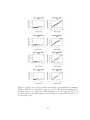
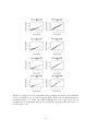
The QQ-plots of the wind power residuals in DK1 and DK2, which compare the empirical distribution of the residuals to the normal distribution, are
presented in Figure 9. The plots indicate that the residual distributions are
slightly skewed and not symmetrical like the normal distribution. The skewness of the residual distributions is in conflict with the model assumption used
for optimizing the model’s log-likelihood, thus parameter estimates may be
suboptimal. The significance of the skewness cannot be rejected in neither
DK1 nor DK2, however, since the skewness is numerically small no further
investigation on the skewness will be conducted. In Figure 10 the residual
empirical distributions are compared to skewed normal distributions.
In conclusion the WP residuals resulting from filtering the first difference
WP series with the specified models can be assumed IID, and in the further
analysis the WP residuals are modeled with the skewed normal distributions.
36
Figure 9: QQ-plots for the WP residuals in DK1 and DK2 under the assumptions of normality.
Figure 10: QQ-plots for the WP residuals in DK1 and DK2 under the assumption of skewed normality. As the skewed normal distribution results in observations forming straight lines, it is concluded that the residuals are slightly
skewed.
37
3.4
Dependence structure and copula fitting
After filtering the series of daily prices and wind power resulting in IID residuals, the dependence structures between the residuals can be investigated.
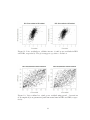
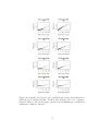
Figure 11 contains plots of the price residuals vs the additive inverse of WP
residuals. The additive inverse is used instead of the WP residual itself, as
it is expected that low wind power is associated with high prices, thus after
changing the sign of the WP residuals, a positive correlation (linear relationship) to the price residuals can be found. When using additive inverse of the
WP residuals the low values of the WP residuals associated with large values
of the price residuals will be found in the upper right corner of the scatterplots. The positive relation is preferred when examining the dependence, in
particular in relation to the extreme dependence, as the relation between the
minimum WP residual and the maximum price residual can be modeled with
the methodology of bivariate maxima introduced in Section 3.5. As expected,
the scatterplots in Figure 11 indicate a positive correlation the price residuals and the additive inverse of the WP residuals in DK1 as well as in DK2.
This relationship will be investigated further in the following sections, in which
bivariate copulas will be fitted to the data.
The five copulas, Normal, Clayton, Gumbel, Frank, and t copula, presented
in Table 1 are fitted to the full sample of the price residuals and the additive
inverse of WP residuals in DK1 and DK2. Three methods are employed:
full maximum likelihood (FML), canonical maximum likelihood (CML) and
inference functions for margins (IFM).
The FML and IFM methods use parametric marginal distribution functions, with which the likelihood of the observations can be evaluated. For
this reason the parametric marginal distribution functions need to be specified. During the fitting of the ARMA-GARCH models to the electricity prices
of DK1 and DK2 in Section 3.2, the price residuals were assumed student-t
distributed. The wind power residuals are assumed to be skewed normally
distributed, as this distribution fits the residuals better than the symmetric
normal distribution according to the conclusion of Section 3.3.1.
In Figure 12 the copula based on empirical (non-parametric) margins in
DK1 and DK2 are presented.
38
Figure 11: Price residuals vs. additive inverse of wind power residuals in DK1
and DK2, respectively. The plots suggest a positive correlation.
Figure 12: Price residual vs. wind power residual using pseudo observations
from empirical (non-parametric) uniform transforms in DK1 and DK2, respectively.
39
Tail correction for price distributions in DK1 and DK2 The assumption of the distribution of the price residuals was validated with the QQ-plots in
Figure 5 for both DK1 and DK2. However, the plots show that the assumption
only holds for the large midsection of the observations and not for the tails as
the t-distribution has flatter tails than the observed distributions of the residuals. Thus assuming t-distribution for the price residuals has the consequence
that the probability of observing the most extreme residual values is numerically zero. The probability of zero results in infinite negative log-likelihood of
the assumed model, which leads to error during the log-likelihood optimization. This error indicates that the specified parametric marginal distribution
is insufficient for capturing the tail behavior, however, since no better fitting
marginal distribution is found, the numerical optimization problem is solved by
correcting the most extreme values in the price residual series. For instance, in
DK1 the residual observation related to the extreme electricity price on June 7,
2013 is replaced. The replacement is based on extreme value theory and done
according to the expected return levels, which allow the replacement values to
be extreme but still occurring with non-zero probability under the assumption
of student-t distribution. The method used for correcting is as follows:
First the most extreme outliers are identified as the observations departing greatly from the 1-1 line in the QQ-plots of the price residuals. For DK1
the outliers include observation 359 (sample minimum) and 523 (sample maximum) and for DK2 observation 31 (sample maximum), 596 (sample’s second
largest value), and 359 (sample minimum).
Using a block length of 15 days, samples of block maxima and block minima
are collected from the full 1080 day sample. GEV distributions are fitted to
the block maxima series and the series of additive inverse of block minima.
Based on the fitted GEV distributions, the expected 1080-day return level is
calculated, and the maximum and minimum observations are replaced with
the expected return levels. The 1080-day return level is defined as the upper
1/1080-quantile of the residual distribution for maximum and lower 1/1080quantile for the minimum. For DK2, where also the second largest observation
needs adjustment, the second largest observation is replaced with the upper
2/1080-quantile, that is the return level for 1080/2=540 days.
40
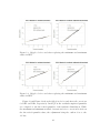
Figure 13: QQ-plot before and after replacing the minimum and maximum
values in DK1.
Figure 14: QQ-plot before and after replacing the minimum and maximum
values in DK2.
Figure 13 and Figure 14 show the QQ-plots before and after tail corrections
for DK1 and DK2, respectively. In the plots the residuals empirical quantiles
are compared to the theoretical quantiles of the student-t distribution. While
the maximum and minimum residual observations before correction lie far from
the theoretical quantile values, the adjustment bring the outliers close to the
1-1 line.
41
It is worth noticing that the altering of the value makes no difference for
the empirical margins used in the CML, as the observations keeps their ranks
in the series.
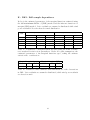
3.4.1
DK1: Dependence structure in West Denmark
DK1
Copula
Parameter
FML
The estimated copula parameters resulting from fitting the five copulas to
residuals from DK1 are presented in Table 11. In this table goodness-of-fit
test results are also shown for each of the copulas and each estimation method.
Marginal function parameters estimated with the FML and IFM methods are
found in Appendix E.
Normal
Clayton
Gumbel
Frank
0.6359 (0.018)
1.106 (0.076)
1.73 (0.05)
4.878 (0.234)
0.6365 (0.018)
49.72 (38.03)
0.63800 (0.01526)
1.06044 (0.06044)
1.67058 (0.04017)
4.8363 (0.2169)
0.63827 (0.01544)
102.652 (137.09)
0.6344 (0.0154)
1.0337 (0.0592)
1.6664 (0.0400)
4.8213 (0.2163)
0.6347 (0.0155)
103.39 (137.80)
CML
t
Normal
Clayton
Gumbel
Frank
IFM
t
Normal
Clayton
Gumbel
Frank
t
Loglikelihood
-2627.334
-2681.599
-2659.486
-2636.792
Goodness-of-fit
Sn
p-value
0.0279
0.08142
0.4784 0.0004995
0.1745 0.0004995
0.0237
0.1204
-2627.74
0.0286
0.07343
278.7
220.3
239.3
269.3
0.0279
0.4784
0.1745
0.0237
0.07842
0.0004995
0.0004995
0.1334
278.6
0.0281
0.06643
278.5
219.2
238.3
269.8
0.0279
0.4784
0.1745
0.0237
0.09441
0.00049
0.00049
0.1124
278.4
0.0286
0.08641
Table 11: DK1: Dependence parameter estimate and goodness-of-fit for copulas when using FML, CML, and IFM. Taken the estimator variance into
consideration, all parameter values agree across estimation method. The copula models are rejected for p-values smaller than 0.05. The Frank copula gives
the best goodness-of-fit regardless of estimation method.
42
Full maximum likelihood The results of the FML estimation show that
all copulas’ dependence parameters are far from those of independence given in
Table 1. The dependence parameter of the normal copula, equal to the linear
correlation parameter, is estimated as 0.64 and is significantly different from
0. This indicates a non-zero, positive correlation between the variables. Table
11 shows the results of the goodness-of-fit test using Sn as the test statistic.
Of the five fitted copulas the Frank, normal and t-copula can not be rejected
as appropriate model at a 95% confidence level. Notice, that the estimated
degrees of freedoms of the t-copula is very high, thus the fitted t-copula is very
similar to the normal copula.
When taking the estimator variance into consideration the estimates of
the parameters of the marginal functions are consistent throughout all copula
models.
Canonical maximum likelihood The dependence parameters agree with
those estimated with FML. Again all parameters are far from the values leading
to independence and the Normal, Frank and t-copula cannot be rejected on a
95% confidence level by the goodness-of-fit test.
Inference functions for marginals Results of the IFM estimation is also
presented in Table 11. As in the previous estimations all parameters are significantly different from the parameters of independence in the respective models.
Moreover, the parameters agree with the values estimated under FML. Again
the result of the goodness-of-fit test shows that Normal, Frank and t-copula
fit well enough not to be rejected on a 95% confidence level.
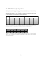
3.4.2
DK2: Dependence structure in East Denmark
The analysis of the dependence between price and wind power in DK2 is equivalent to the one of DK1.
Following the same procedure as in the previous section the five copulas
in Table 1 are fitted to the full sample data of price residuals and WP residuals. Main results are presented in Table 12 and the estimated parameters of
marginal functions using FML and IFM are presented in Appendix F.
43
DK2
Copula
Parameter
FML
Normal
Clayton
Gumbel
Frank
0.5803 (0.02)
0.9498 (0.07)
1.597 (0.045)
4.206 (0.222)
0.5813 (0.021)
48.39 (35.85)
0.5852 (0.0174)
0.9064 (0.0566)
1.554 (0.0370)
4.180 (0.2083)
0.5844 (0.01756)
111.87 (209.33)
0.5793 (0.0175)
0.8984 (0.0559)
1.543 (0.0366)
4.165 (0.2076)
0.5798 (0.0177)
101.48 (133.73)
CML
t
Normal
Clayton
Gumbel
Frank
IFM
t
Normal
Clayton
Gumbel
Frank
t
Loglikelihood
-2723.359
-2761.503
-2757.028
-2731.662
Goodness-of-fit
Sn
p-value
0.0249
0.1364
0.3432 0.0004995
0.1856 0.0004995
0.0271
0.06543
-2723.762
0.0256
0.1404
222.3
179.3
185.8
212.9
0.0249
0.3432
0.1856
0.02171
0.1424
0.00050
0.00050
0.0764
222.2
0.0257
0.1284
221.6
180.3
181.6
213.6
0.0249
0.3432
0.1856
0.0271
0.1324
0.00050
0.00050
0.06943
221.5
0.0256
0.1264
Table 12: DK2: Dependence parameter estimates and goodness-of-fit for copulas found with the three methods FML, CML, and IFM. Taken the estimator variance into consideration all parameter values agree across estimation
method. The Normal copula gives the best goodness-of-fit. Neither Normal,
Frank and t-copula can be rejected on a 95% confidence level.
Full maximum likelihood All dependence parameters estimated with FML
are far from the parameter values leading to independence, and the non-zero
dependence parameter of the normal copula indicates significant correlation
between the variables. The Normal, Frank and t-copula can not be rejected
by the goodness-of-fit test at a 95% confidence level. The Normal copula gives
the highest log-likelihood and the best goodness-of-fit.
The parameters of the marginal distribution functions are consistent across
choice of copula model taking the variance of the estimates into considerations.
Canonical maximum likelihood The canonical maximum likelihood gives
parameter estimates as in Table 12, which also shows the goodness-of-fit test
results. The dependence parameters are similar to the ones estimated with
44
FML. Again Gumbel and Clayton copula can be rejected at a 95% confidence
level, while Normal, Frank and t-copula cannot be rejected according to the
goodness-of-fit test.
Inference functions for marginals All values resulting from the IFM estimation are consistent with the FML estimates. As with the two other estimation method all dependence parameters are far from those values leading to
independence. Normal, Frank and t-copula cannot be rejected 95% confidence
level.
3.4.3
Likelihood-ratio test for Normal copula
The likelihood-ratio test is applied to the copula based on empirical marginal
functions (see the estimation results under CML method).
For DK1 the log-likelihood of the normal copula is 278.73 and the loglikelihood of independence copula is 2.418e-13. The resulting test statitics as
defined in (19) is 557.46, and this is much greater than 3.84, which is the 95%
upper quantile of the χ2 (1) distribution. The test rejects the null hypothesis
of independence.
The log-likelihood of the normal copula fitted to the empirical pseudo observations of DK2 is 222.33, while the log-likelihood of the independence copula
is 2.551e-13. This results in a test statistic with the value 444.67, witch is
greater than the 95% upper quantile of the χ2 (1) distribution, thus the test
rejects the hypothesis of independence.
The likelihood-ratio test confirms the idea that there exists significant dependence between the price residuals and the additive inverse of WP residuals.
3.4.4
Discussion on full sample dependence
The results of the copula and marginal function fitting for the price residuals
and WP residuals in DK1 as well as in DK2 indicate a significant dependence
between the price residual and WP residuals. Moreover, for DK1 the Frank
copula has the highest likelihood and highest goodness-of-fit p-value for most
of the used estimation methods. The Normal copula gave the best goodnessof-fit for the data of DK2. The degrees-of-freedom of the t-copula is very large
for both DK1 and DK2 regardless of estimation method, and as the t-copula
45
converges toward the Normal copula as the degrees-of-freedom approaches infinity, the fitted t-copulas are very similar to the Normal copula. This explains
the large goodness-of-fit of the t-copula as well as the dependence parameter
of the t-copula being very close to the dependence parameter of the normal
copulas.
Since the first difference is used for modeling the prices as well as the WP,
the residuals express an excess change in price and WP. The significant dependence between price residual and WP residual can accordingly be interpreted
as excess increase in wind power production leads to an excess decrease of
the price, while excess decrease in wind power production leads to excess increase of the price. This result is expected. Wind power has low marginal cost
compared to other kinds of power generation methods, and high wind power
production should therefore lead to low electricity prices, while low production
should lead to higher electricity prices.
The dependence parameter of the Normal copula, which is equal to the
linear correlation coefficient, is around 0.63 in DK1 while it is 0.58 in DK2,
and both values are significant according to the likelihood-ratio test. However, the difference between the correlation estimated for the two areas is not
statistically significant.
In the next section the extreme dependence will be investigated. Accepting
the Normal and Frank copula as appropriate models for the full sample dependence, an idea about the extreme dependence can already be established using
the definition of upper tail dependence given in equation (12). The extreme
dependence of the Normal copula can be shown to be zero, except in the case
of perfect dependence. Likewise, the Frank copula has upper tail dependence
of zero.
46
3.5
Estimation of extreme value copula and extreme dependence structure
The results of the investigation of extreme dependence, that is the dependence
between the maximum values of the price residuals and additive inverse of WP
residuals, are presented in this section. It should be noted that for this analysis
the price residual series without tail corrections are used.
First an appropriate block length is identified in order to collect a componentwise block maxima sample from the full sample. A short block length gives
a large sample which in return gives small variance of the estimates, however,
the results may be biased as the sample does not represent the maximum well.
On the other hand, a large block length gives only a few observations thus
may result in large variance. The block length is chosen for DK1 and DK2
as the shortest length for which both block maxima price residuals and block
maxima WP residuals seem to fit the generalized extreme value distribution
well. For DK1 the block length is set to 20 days and for DK2 40 days, and the
reason behind choosing these particular block lengths can be found under the
analysis of the respective areas.
Figure 15: Block maxima price residuals vs block maxima wind power residuals
of DK1 and DK2, respectively. The sample of DK1 has more observations than
DK2 due to the shorter block length. Observe, that x-axis in the DK1-plot
has been cropped such that maximum price residual is outside the plot.
47
Figure 16: Non-parametric uniform transform of the block maxima price residual vs wind power residual in DK1 and DK2, respectively. For DK1 a 20 days
block length is chosen while the block length is set to 40 days for DK2.
In Figure 15 the componentwise block maxima (BM) of price residual vs
additive inverse of WP residuals in DK1 and DK2 are plotted. The corresponding scatterplots of the non-parametric uniform transform are shown in
Figure 16.
3.5.1
DK1: Extreme dependence in West Denmark
The block length is chosen by investigating the QQ-plots of GEV distributions
fitted to block maxima of different block lengths. In Figure 17 the QQ-plot
for block maxima price residuals as well as block maxima WP residuals are
shown for block length of 10, 20, 30 and 40 days. Larger block lengths than 40
days will result in very few observations, thus are not considered. The block
maxima of WP residuals seem to follow GEV distribution for block length 20,
and the price residual block maxima follow a GEV-distribution for any choice
of block length with the exception of maximum observation of price residuals,
which is much higher than expected under the GEV-assumption. This applies
for any of the chosen block lengths. Hence, the block length is set to 20 days
as neither shorter nor longer block lengths offer improvements to the fit.
48
Figure 17: QQ-plots for price residuals and wind power residuals block maxima
(BM) in DK1 for block lengths 10, 20, 30, and 40. While the maximum price
residual seems to lie outside the GEV distribution for all of the plotted block
lengths, the block maxima wind power residuals follow the GEV already for a
block length of 20.
49
Figure 18: Density plots comparing the density of the fitted GEV distribution
to the empirical density of the 20-day block maxima of price residuals and and
WP residuals in DK1.
The block length of 20 days result in 54 block maximum observations. In
Figure 18 the density function of the fitted GEV distributions are plotted and
compared with the empirical density of the 20-day block maxima. The plots
suggest that the block maxima reasonably can be assumed to follow the GEV
distributions.
Copula parameters estimated with the FML, CML and IFM methods can
be found in Table 13 together with goodness-of-fit test results. Estimated GEV
parameters of the margins can be found in Appendix G.
Full maximum likelihood Results of the FML estimation of GEV distributions of margins and the various extreme value copulas indicate that dependence parameters are very close to the parameter values leading to independence. None of the copula models can be rejected on a 95% confidence level
according to both the goodness-of-fit test based on Sn , and the goodness-of-fit
test for extreme value copulas with test statistic Mn .
Moreover, the parameters of the marginal GEV distributions agree throughout all four copula models when taking estimator variance into consideration.
Canonical maximum likelihood CML fitting of extreme value copulas to
observations in DK1 results in parameter estimates similar to those of the
50
Copula
Parameter
Loglikelihood
FML
Gumbel
Tawn
Husler-Reiss
Galambos
1.13 (0.132)
0.21 (0.36)
0.50 (0.272)
0.27 (0.17)
-84.17
-84.43
-84.10
-84.03
IFM
CML
DK1
Gumbel
Tawn
Husler-Reiss
Galambos
Gumbel
Tawn
Husler-Reiss
Galambos
1.1395
0.2678
1.1392
0.3958
1.0668
0.1579
0.5108
0.2551
(0.1153)
(0.2482)
(0.1152)
(0.1387)
(0.1018)
(0.2786)
(0.2200)
(0.1622)
0.9174
0.5425
0.9174
1.109
0.2439
0.1508
0.1386
0.1729
Goodness-of-fit p-value
Sn -test
Mn -test
0.5779
0.2782
0.3561
0.1434
0.6538
0.3182
0.5989
0.3122
0.5629
0.2542
0.3731
0.1673
0.6908
0.3082
0.6139
0.3112
0.55
0.2612
0.3851
0.1703
0.6858
0.3292
0.6159
0.2822
Table 13: Goodness-of-fit test results for extreme value copulas fitted to BM
of DK1 using FML, CML, and IFM. None of the models can be rejected on a
95% confidence level as all p-values are greater than 0.05.
FML estimation. Likewise, the CML gives parameter estimate close to the
parameter values of the independence copula. While none of the models can
be rejected on a 95% confidence level, the Galambos copula has the highest
log-likelihood.
Inference functions for marginals The estimation results using the IFM
method are similar to those of the other two methods. Parameters are close
to the values leading to independence. As for the other estimation methods
the Tawn copula gives the worst goodness-of-fit, however, none of the copula
models can be rejected.
3.5.2
DK2: Extreme dependence in East Denmark
For the data series of DK2, the block length is set to 40 days and this choice
is based on the following analysis.
In Figure 19 the QQ-plot for block maxima price residuals as well as block
maxima WP residuals are shown for block length of 10, 20, 30 and 40 days.
Figure 20 show the return level plots for same blocklengths.
51
Figure 19: QQ-plots for block maxima price residuals and wind power residuals
for block length 10, 20, 30 and 40 days in DK2. While the two maximum price
residuals seem to lie outside the GEV distribution for all of the plotted block
lengths, the block maxima wind power residuals follow the GEV already for a
block length of 10.
52
Figure 20: Return level plots for price residuals and wind power residuals for
different block lengths in DK2. Dashed lines indicates the 95% confidence
interval. Only for the block length of 40 days the maximum price residual lies
within the confidence interval.
53
Figure 21: Density plots comparing the density of the fitted GEV distribution
to the empirical density of the 40-day block maxima of price residual and and
WP residual in DK2.
Since block lengths larger than 40 days will result in very few observations
such block lengths are not considered. By investigating the QQ-plots of GEV
distributions fitted to block maxima of different block lengths, a reasonable
block length can be determined. The block maxima of WP residuals seem
to follow GEV distribution for any choice of block length. The two maximum
values of the price residual block maxima are higher than expected for all block
lengths, indicating that the fitted GEV distributions do not capture the tail
behavior. However, the return level plots show that for the block length of 40
days the two maximum observation lie within the 95% confidence interval of
the return level. This is not the case for shorter block lengths and with this
reason the block length is set to 40 days. The block length of 40 days result
in 27 block maximum observations. The density functions of the fitted GEV
are plotted and compared with empirical density of the 40-day block maxima
in Figure 21.
Estimated copula parameters found using FML, CML and IFM methods
are presented in Table 14 together with goodness-of-fit test results. Estimated
GEV parameters of the margins can be found in Appendix G.
54
IFM
CML
FML
DK2
Copula
Parameter
Gumbel
Tawn
Husler-Reiss
Galambos
Gumbel
Tawn
Husler-Reiss
Galambos
Gumbel
Tawn
Husler-Reiss
Galambos
1.13 (0.148)
0.4 (0.378)
0.772 (0.247)
0.445 (0.199)
1.232 (0.193)
0.4518 (0.3489)
0.8964 (0.2683)
0.5065 (0.2114)
1.176 (0.1565)
0.3415 (0.3570)
0.8063 (0.2258)
0.4371 (0.1760)
Loglikelihood
-38.415
-38.885
-38.525
-38.138
0.9484
0.7131
1.113
1.062
0.8943
0.3912
1.199
1.114
Goodness-of-fit p-value
Sn -test
Mn -test
0.03946
0.5939
0.03047
0.484
0.05045
0.6878
0.05544
0.6479
0.03846
0.6069
0.02847
0.5
0.04545
0.6968
0.05544
0.6299
0.04046
0.5829
0.02348
0.525
0.05544
0.6998
0.04046
0.6119
Table 14: Goodness-of-fit test results for extreme value copulas fitted to BM
of DK1 using FML, CML and IFM. None of the models can be rejected on
a 95% confidence level by the Mn -test as all p-values are greater than 0.05.
However, the Sn -test produces low p-values for all copulas and rejects Gumbel
and Tawn copula for all estimation methods.
Full maximum likelihood Dependence parameters estimated by FML do
not clearly differ from the parameter values leading to independence. None
of the copula models can be rejected on a 95% confidence level according to
the goodness-of-fit test for extreme value copulas with test statistic Mn , however the Sn -test rejects Gumbel and Tawn copula. Test results are presented
together with estimated copula parameter values in Table 14. Estimated parameter of the GEV distributions fitted to margins can be found in Appendix
H, and the results show that the parameters of the marginal distribution function agree throughout all four copula models.
Canonical maximum likelihood The results of the CML fitting of extreme
value copula to the observations in DK2 are also presented in Table 14. As
the FML estimation the CML gives parameter estimate close to the parameter
values of the independence copula. The Gumbel, Tawn, and Husler-Reiss
copula are rejected by the S n -test on a 95% confidence level while the M n -test
does not reject any of the models.
55
Inference functions for marginals The estimation results using the IFM
method are similar to those of the other two methods. Parameters are close
to the values leading to independence and the Husler-Reiss copula gives the
highest log-likelihood and p-values in the goodness-of-fit tests, however, none
of the models can be rejected according to the Mn -test. The Sn -test rejects all
but the Husler-Reiss copula on a 95% confidence level.
56
3.5.3
χ-plots and χ-plots
¯
The χ-plot and χ-plot
¯
for DK1 is presented in Figure 22. With the χ(u)
function value significantly above zero the idea of positive dependence between price residual and additive inverse of wind power residual is supported.
According to the theory of the plots presented in Section 2.3.5 upper tail independence exists if χ(u) → 0 for u → 1. The χ-plot does show decreasing
function value, however, it is not possible to determine whether function limits
to zero or instead to a positive value near zero. In the χ-plot,
¯
on the other
hand, it is clear that χ(u)
¯
does not limit to 1 as u → 1. This gives a strong
indication of asymptotic independence.
χ-plot and χ-plot
¯
constructed on the basis of the price residual block maxima and wind power residual block maxima are presented in Figure 23. The
functions have large variances, due to the few observations. The χ-plot does
not reject the assumption of the maxima being independent as the χ(u)function does not significantly depart from 0. Moreover, the χ(u)
¯
is very
far from 1 as u → 1 thus there is no indication of upper tail dependence.
Like the χ-plot and χ-plot
¯
for DK1 the plots for DK2 indicate a significant
dependence between the price residuals and the wind power residuals. The
χ-plot and χ-plot
¯
for DK2 can be found in Figure 24. The χ(u) function value
is greater than zero for all u, however, the function is decreasing and reaching
values close to 0 for u → 1, which indicates asymptotic independence. χ(u)
¯
is smaller than 1 for u → 1, thus the χ-plot
¯
supports the idea of asymptotic
independence.
In Figure 25 the χ-plot and χ-plot
¯
for the price and wind power residual
block maxima can be found. Here, the χ(u) function value is not significantly
different from 0 for any value of u, thus independence between the maxima
is indicated. Long block length and few observations result in large estimate
variances, thus reaching conclusion on the basis of the block maxima χ-plot
and χ-plot
¯
is not possible. E.g. asymptotic independence cannot be rejected
as 1 lies side the confidence interval of χ(u)
¯
for u → 1 .
57
Figure 22: χ-plot and χ-plot
¯
for DK1. Dashed lines indicates the 95% confidence interval. The χ(u) function value is greater zero for all u, indicating
a clear and positive relationship between the price residual and the additive
inverse wind power residual. However, the χ(u)
¯
is smaller than 1 for u → 1,
which means asymptotic independence.
Figure 23: χ-plot and χ-plot
¯
for price and WP residual block maxima in
DK1. Dashed lines indicates the 95% confidence interval. χ(u) is close to
0 for all values of u, indicating independence between the price residual and
the additive inverse wind power residual. Likewise, χ(u)
¯
is is different from 1
for u → 1, which means asymptotic independence. Large estimate variation
impede reaching conclusions based on the plots, however, no clear sign of
dependence nor asymptotic dependence exists.
58
Figure 24: χ-plot and χ-plot
¯
for DK2. Dashed lines indicates the 95% confidence interval. The χ(u) function value is greater than zero for all u, indicating
a positive relationship between the price residual and the additive inverse wind
power residual. However, the χ(u)
¯
is smaller than 1 for u → 1, which supports
the idea of asymptotic independence.
Figure 25: χ-plot and χ-plot
¯
for price and WP residual block maxima in DK2.
Dashed lines indicates the 95% confidence interval. Due to large variance of
the functions conclusions regarding dependence and asymptotic dependence
are difficult to reach.
59
3.5.4
Discussion on extreme value dependency
The results of the copula and marginal function fitting for the block maxima
indicate that no significant dependence between the maximum price residual
and maximum additive inverse of WP residuals exists in neither DK1 nor DK2.
In other words, the extreme excess increases in price appear independent from
the extreme excess decreases in the produced WP. The conclusion is supported
with the estimated dependence parameter values of the copulas, which all lie
close to the values leading to independence. None of the fitted copulas could
be rejected by the Sn goodness-of-fit test. This result could be explained
by independent observations, as copulas similar to the independence copula
would not be rejected if observations are independent. Moreover, the extreme
independence is supported by the χ-plots and χ-plots
¯
for the full sample, which
exhibit upper tail independence for both DK1 and DK2. Despite large estimate
variation, the chi-plots of the block maxima indicate independence for the block
maxima, which is equivalent to upper tail independence.
While the results of the full sample copula modeling show positive dependency between price and WP residuals, results of the extreme value copula
fitting indicate that the maxima occur independently.
60
4
Conclusion
In this chapter the results of the investigation of the dependence structure
presented in Section 3 are summarized and conclusion in relation to the overall
research questions is reached.
4.1
Summary of results
The results of the four steps of this study including price series filtering, wind
power series filtering, modeling of full sample dependence, and modeling of
extreme dependence, is presented below.
1. The day-ahead daily power prices are filtered using an ARMA-GARCH
model with weekday indicator variables under the assumption of t-distributed
residuals. While the optimal order of the model for the prices of DK1
is ARMA(3,3)-GARCH(1,1), the optimal model for DK2 is ARMA(4,3)GARCH(1,1). The models successfully remove autocorrelation and heteroscedasticity from the price series.
2. The daily wind power is filtered using an ARMA-GARCH model. The
optimal model of for the wind power in DK1 is ARMA(1,2)-GARCH(1,1)
and for the series in DK2 ARMA(3,3)-GARCH(2,3) under the assumption of normally distributed residuals. The models remove all autocorrelation and heteroscedasticity, however, residuals are slightly skewed.
3. Copula fitting to the observations of price residuals and WP residuals
in DK1 as well as in DK2 indicate a significant dependence between
the price and WP residuals. The Normal and Frank copulas have the
highest likelihood and highest goodness-of-fit p-value, while the t-copula
could also not be rejected. Linear correlation coefficients between price
residuals and additive inverse wind power residuals are significant and
positive.
4. Extreme value modeling using block maxima with block lengths of 20 and
40 for DK1 and DK2, respectively, indicates asymptotic independence.
None of the fitted copulas could be rejected using the Mn -test, however,
all dependence parameters are close to those of independence. χ-plots
and χ-plots
¯
support upper tail independence.
61
4.2
Conclusion
The results of the study can lead to the following conclusions for both DK1
and DK2:
• There exist a clear relation between the day-ahead electricity price and
the daily wind power production, such that low production is associated
with high price. The most appropriate models for the dependency between filtered wind power production and filtered prices is the Normal
copula alternatively the Frank copula.
• Extremely low wind power in-feed does not cause extremely high dayahead electricity prices due to asymptotic independence. That is, extremely low wind power production occur independently from extremely
high prices thus low wind power production can not explain the occurrence of extreme prices.
While there is a significant relation between excess wind power production and
excess electricity prices, no significant relation between prices and wind power
production under extreme conditions in neither DK1 nor DK2 was found. The
results imply that the Danish power market so far has seen the positive price
effects of the wind power, as excess wind power production leads to lower
prices. At the same time the lack of asymptotic dependence show that low
wind power production does not lead to extreme prices, as the extremely high
prices appear uncorrelated with extremely low wind power production. While
previous studies show that wind power increases electricity price volatility, this
study suggests that it does not cause price spikes, as the upper tail-behavior
of the electricity prices remains independent from the wind power production.
In conclusion, the Danish power market with its wind power share of more
than 30% of the generated electricity does not experience wind power as the
cause of extreme day-ahead prices, thus the large share of wind power is not
challenging the stability of the day-ahead market in terms of extremely high
prices.
62
References
Beirlant, J. et al (2004) Statistics of Extremes: Theory and Applications. 1st ed. Wiley
Capéraà, Faugeres and Genest (1997) A nonparametric estimation procedure for bivariate
extreme value copulas. Biometrika. Volume 84:3, pages 567-577
Coles, S. (2001) An Introduction to Statistical Modeling of Extreme Values.
Springer-Verlag London
Coles, S., Heffernan, J. and Tawn, J. (1999) Dependence Measures for Extreme Value
Analyses. Extremes 1999, Volume 2:4, pages 339-365.
Cryer, J. D. and Chan, K. (2008) Time Series Analysis With Applications in R. Springer
Scienge+Business.
Ea Energianalyse A/S (2005) 50 pct. vindkraft i Danmark i 2025 - en teknisk-økonomisk
analyse. http://energinet.dk [visited 2015.04.20]
Fisher, T. J. and Gallagher, C. M. (2012) New Weighted Portmanteau Statistics for Time
Series Goodness of Fit Testing. Journal of the American Statistical Association. Volume
107:498
Genest, C. et al (2011) A goodness-of-fit test for bivariate extreme-value copulas.
Bernoulli. Volume 17:1, pages 253-275
Genest, C., Quessy, J. and Rémillard, B. (2006) Goodness-of-fit Procedures for Copula
Models Based on the Probability Integral Transformation. Scandinavian Journal of
Statistics. Volume 33:2, pages 337-366
Gudendorf, G., and Segers, J. (2009) Extreme-Value Copulas.
Joe, H. and Xu, J.J. (1996). The estimation method of inference functions for margins for
multivariate models. Technical Report. no. 166. Department of Statistics, University of
British Columbia
63
Ketterer, Janina C. (2014) The impact of wind power generation on the electricity price in
Germany. Energy Economics. Volume 44, July, pages 270–280
Kojadinovic, Yan and Holmes (2011) Fast large-sample goodness-of-fit tests for copulas.
Statistica Sinica. Volume 21:2, pages 841-871
Lindström, E. and Regland, F. (2012) Modeling extreme dependence between European
electricity markets. Energy Economics. Volume 34:4, pages 899-904
Nelsen, R. B. (2004) An Introduction to Copulas. 2nd ed.
Nord Pool Spot (n.d.) About us. Available from:
http://www.nordpoolspot.com/About-us/ [visited 2015.04.20]
Nord Pool Spot (2013) Central to European Power Integration - Annual Report.
Nord Pool Spot (n.d.) Day-ahead market elspot. Available from:
http://www.nordpoolspot.com/TAS/Day-ahead-market-Elspot/ [visited 2015.04.20]
NordReg (2014) An overview of the Nordic Electricity Market. Available from:
http://www.nordicenergyregulators.org/about-nordreg/an-overview-of-the-nordicelectricity-market/ [visited
2015.04.20]
Paraschiv, Erni and Pietsch (2014) The impact of renewable energies on EEX day-ahead
electricity prices. Energy Policy. Volume 73, October, pages 196–210
Rasmussen, J. N. (2013) Vestdanmark får fredag høje elpriser i fem timer. Available from:
http://energinet.dk/DA/El/Nyheder/Sider/Vestdanmark-faar-fredag-hoeje-elpriser-i-femtimer.aspx [visited
2015.04.20]
Aloui, R. et al (2014) Dependence and extreme dependence of crude oil and natural gas
prices with applications to risk management. Energy Economics. Volume 42, March pages
332-342
64
Appendix
A - DK1: Price filtering
(a) First difference of daily electricity prices in
DK1.
(b) Standardized price residual for DK1 after
fitting the ARMA(3,3)-GARCH(1,1) model
with weekday indicators to first difference of
prices.
(c) Sample ACF of the price residuals
in DK1 resulting from fitting ARMA(3,3)GARCH(1,1) model with weekday indicator
variables to the price series. The dashed lines
indicates the threshold for 95% significance
level. No significant autocorrelation is seen.
(d) Sample ACF of the squared price residuals
in DK1 resulting from fitting an ARMA(3,3)GARCH(1,1) model to the price series. The
dashed lines indicate the threshold for 95% significance level. No significant autocorrelation
can be identified thus no heteroscedasticity.
Figure 26: DK1: Price filtering
65
B - DK2: Price Filtering
(a) First difference of daily electricity prices in
DK2.
(b) Standardized price residual for DK2 resulting from fitting an ARMA(4,3)-GARCH(1,1)
model with weekday indicator variables to first
difference of prices.
(c) Sample ACF of the price residual in
DK2 resulting from fitting an ARMA(4,3)GARCH(1,1) model to the price series. As no
ACF values surpass the dashed line, which indicates the threshold of significance at a 95%
confidence level, no significant autocorrelation
can be identified.
(d) ACF of the squared price residuals
in DK2 resulting from fitting ARMA(4,3)GARCH(1,1) model with weekday indicator
variables to the first difference price series.
The dashed line indicates the threshold for significance at a 95% confidence level. There is
no indication of significant autocorrelation as
no ACF values surpass the threshold, and the
residuals can be assumed homoscedastic.
Figure 27: DK2: Price filtering
66
C - DK1: Wind Power Filtering
(a) First difference of daily wind power produced in DK1. The series is assumed stationary as the KPSS test can not reject the stationarity hypothesis on a 95% confidence level.
(b) Daily wind power residual in DK1.
(c) Sample ACF of the daily wind power residual in DK1. No significant autocorrelation can
be found in the residuals, as no ACF-values
surpass the dashed lines, which indicates the
95%-significance level.
(d) ACF of the squared wind power residual
in DK1. The dashed lines indicate the significance threshold at a 95% confidence level. No
significant autocorrelation can be seen in the
plot, indicating no further heteroscedastic effects exist in the residuals.
Figure 28: DK1: Wind power filtering
67
D - DK2: Wind Power Filtering
(a) First difference of daily wind power produced in DK2.
(b) Daily wind power residuals in DK2.
(c) Sample ACF of the daily wind power residual in DK2. The dashed line indicates the
threshold of significance on a 95% confidence
level. No significant autocorrelation is identified, as no ACF-value for non-zero lags surpass
the threshold.
(d) Sample ACF of the squared daily wind
power residuals in DK2. As no values surpass
the 95% significance level threshold indicated
with the dashed line, homoscedasticity in the
residuals can be assumed.
Figure 29: DK2: Wind power filtering
68
E - DK1: Full sample dependence
Below is the estimated parameters of the marginal functions estimated using
the full maximimum likelihood (FML) method and the inference functions for
margins (IFM) method. Price residuals are assumed t-distributed while wind
power residuals follow the skewed normal distribution.
DK1
Normal
Clayton
Gumbel
Frank
t
Marginal function (Price)
Mean
SD
DF
0.0098 (0.024)
0.988 (0.053)
3.659 (0.421)
Marginal function (WP)
Mean
SD
Skew
-0.0053 (0.029)
0.996 (0.022)
0.720 (0.030)
0.0505 (0.024)
1.105 (0.087)
3.071 (0.319)
0.0165 (0.029)
1.02 (0.021)
0.649 (0.028)
-0.0059 (0.024)
1.072 (0.075)
3.239 (0.353)
-0.0088 (0.029)
1.01 (0.022)
0.803 (0.033)
0.0075 (0.023)
0.955 (0.040)
4.382 (0.603)
-0.0110 (0.029)
1.01 (0.023)
0.692 (0.031)
0.0099 (0.024)
0.985 (0.053)
3.685 (0.428)
-0.0052 (0.029)
0.997 (0.022)
0.721 (0.030)
Table 15: Parameters of marginal functions when using the FML. Parameters’ standard deviation is in parentheses. Under all copula assumptions, the
estimated parameters of the marginal functions agree, taking the estimate
variation into consideration.
Marginal function (price)
Mean
SD
DF
0.01256 0.9566 4.175
Marginal function (WP)
Mean
SD
Skew
-0.009024 0.9989 0.6981
Table 16: Parameter values estimated with IFM method for the observations
in DK1. Price residuals are assumed t-distributed, while wind power residuals
are skewed normal.
69
F - DK2: Full sample dependence
Below is the estimated parameters of the marginal functions estimated using
the full maximimum likelihood (FML) method and the inference functions for
margins (IFM) method. Price residuals are assumed t-distributed while wind
power residuals follow the skewed normal distribution.
DK2
Normal
Clayton
Gumbel
Frank
t
Marginal function (Price)
Mean
SD
DF
Marginal function (WP)
Mean
SD
Skew
0.0054 (0.026)
0.976 (0.039)
4.5837 (0.610)
0.0013 (0.029)
0.997 (0.022)
0.711 (0.029)
0.0407 (0.025)
1.048 (0.055)
3.7557 (0.445)
0.0171 (0.029)
1.012 (0.021)
0.655 (0.028)
-0.0005 (0.026)
1.046 (0.053)
3.8830 (0.478)
0.0017 (0.030)
1.009 (0.022)
0.779 (0.032)
0.0022 (0.025)
0.968 (0.034)
5.2420 (0.807)
-0.0061 (0.030)
1.010 (0.023)
0.689 (0.030)
0.0064 (0.026)
0.977 (0.039)
4.5894 (0.616)
0.0018 (0.029)
0.998 (0.022)
0.711 (0.029)
Table 17: Parameters of the marginal functions estimated using the FML.
Standard deviation of parameter estimates is given in parentheses.
Marginal function (price)
Mean
SD
DF
0.01239 0.9653 5.0206
Marginal function (WP)
Mean
SD
Skew
0.00299 0.9993 0.6879
Table 18: Parameter values estimated with IFM method for observations in
DK2. Price residuals are assumed t-distributed, while wind power residuals
are skewed normal.
70
G - DK1: Extreme dependence
Below is the estimated parameters of the marginal functions estimated using
the full maximimum likelihood (FML) method and the inference functions for
margins (IFM) method. Both block maxima of price residuals and wind power
residuals are assumed to be GEV distributed.
DK1
Gumbel
Tawn
Husler-Reiss
Galambos
Marginal function (Price)
Location
Scale
Shape
Marginal function (WP)
Location
Scale
Shape
1.362 (0.082)
0.543 (0.069)
0.324 (0.091)
1.448 (0.053)
0.346 (0.037)
-0.193 (0.093)
1.372 (0.089)
0.567 (0.083)
0.351 (0.105)
1.428 (0.052)
0.329 (0.034)
-0.128 (0.103)
1.362 (0.081)
0.543 (0.068)
0.324 (0.096)
1.448 (0.053)
0.346 (0.037)
-0.193 (0.097)
1.358 (0.082)
0.545 (0.069)
0.347 (0.096)
1.449 (0.053)
0.346 (0.037)
-0.191 (0.096)
Table 19: Estimated parameter for marginal functions FML. The block maxima observations are from DK1. Parameter estimates’ standard variations are
given in parentheses.
DK1
Price residual BM
WP residual BM
Marginal functions
Location Scale
Shape
1.3621
0.5425 0.3240
1.4484
0.3458 -0.1927
Table 20: Parameter values of marginal functions estimated with IFM method
for observations from DK1.
71
H - DK2: Extreme dependence
Below is the estimated parameters of the marginal functions estimated using
the full maximimum likelihood (FML) method and the inference functions for
margins (IFM) method. Both block maxima of price residuals and wind power
residuals are assumed to be GEV distributed.
DK2
Gumbel
Tawn
Husler-Reiss
Galambos
Marginal function (Price)
Location
Scale
Shape
Marginal function (WP)
Location
Scale
Shape
1.852 (0.114)
0.524 (0.104)
0.428 (0.169)
1.654 (0.059)
0.256 (0.047)
0.097 (0.214
1.852 (0.115)
0.524 (0.106)
0.428 (0.165)
1.654 (0.059)
0.256 (0.047)
0.097 (0.211)
1.830 (0.114)
0.552 (0.119)
0.359 (0.163)
1.653 (0.060)
0.244 (0.043)
0.123 (0.214)
1.848 (0.114)
0.524 (0.105)
0.451 (0.177)
1.654 (0.059)
0.255 (0.047)
0.101 (0.214)
Table 21: Estimated parameters for marginal functions using FML. The block
maxima observations are from DK2. Parameter estimates’ standard variations
are given in parentheses.
DK2
Price residual BM
WP residual BM
Marginal functions
Location Scale Shape
1.852
0.523 0.427
1.654
0.256 0.0968
Table 22: Marginal function parameter values estimated with IFM method for
observations from DK2.
72