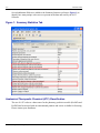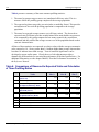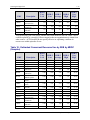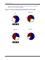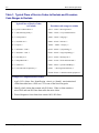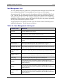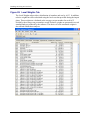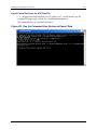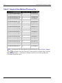
1
The Johns Hopkins
ACG System
®
Technical User Guide
Version 8.2
December 2008
This page is intentionally left blank.
Important Warranty Limitation and Copyright Notices
Copyright 2008, The Johns Hopkins University. All rights reserved.
This document is produced by the Health Services Research & Development Center at
The Johns Hopkins University, Bloomberg School of Public Health.
The terms The Johns Hopkins ACG® System, ACG® System, ACG®, ADG®, Adjusted
Clinical Groups®, Ambulatory Care GroupsTM, Aggregated Diagnostic GroupsTM,
Ambulatory Diagnostic GroupsTM, Johns Hopkins Expanded Diagnosis ClustersTM,
EDCsTM, ACG Predictive Model™, Rx-Defined Morbidity Groups™, Rx-MGs™, ACG
PM™, Dx-PM™, Rx-PM™ and DxRx-PM™ are trademarks of The Johns Hopkins
University. All materials in this document are copyrighted by The Johns Hopkins
University. It is an infringement of copyright law to develop any derivative product
based on the grouping algorithm or other information presented in this document.
This document is provided as an information resource on measuring population morbidity
for those with expertise in risk-adjustment models. The documentation should be used
for informational purposes only. Information contained herein does not constitute
recommendation for or advice about medical treatment or business practices.
No permission is granted to redistribute this documentation. No permission is granted to
modify or otherwise create derivative works of this documentation.
Copies may be made only by the individual who requested the documentation initially
from Johns Hopkins or their agents and only for that person's use and those of his/her coworkers at the same place of employment. All such copies must include the copyright
notice above, this grant of permission and the disclaimer below must appear in all copies
made; and so long as the name of The Johns Hopkins University is not used in any
advertising or publicity pertaining to the use or distribution of this software without
specific, written prior authorization.
Disclaimer: This documentation is provided AS IS, without representation as to its
fitness for any purpose, and without warranty of any kind, either express or implied,
including without limitation the implied warranties of merchantability and fitness for a
particular purpose. The Johns Hopkins University and the Johns Hopkins Health System
shall not be liable for any damages, including special, indirect, incidental, or
consequential damages, with respect to any claim arising out of or in connection with the
use of the documentation, even if it has been or is hereafter advised of the possibility of
such damages.
Documentation Production Staff
Senior Editor: Jonathan P. Weiner, Dr. P.H.
Managing Editor: Chad Abrams, M.A.
Production assistance provided by: David Bodycombe Sc.D., Klaus Lemke, Ph.D.,
Patricio Muniz, M.D., MPH, MBA, Thomas M. Richards, Barbara Starfield, M.D., MPH
and Erica Wernery.
Special thanks to Lorne Verhulst M.D., MPA, of the British Columbia Ministry of Health
in Vancouver, Canada, for his contribution to the chapter titled Practitioner Profiling:
Assessing Individual Physician Performance Provider Performance Assessment.
Additional production assistance and original content provided by Rosina DeGiulio,
Meg McGinn, and Amy Salls of DST Health Solutions, LLC. The ACG Team gratefully
acknowledges the support provided by our corporate partner in helping to move this
publication forward.
If users have questions regarding the software and its application, they are advised to
contact the organization from which they obtained the ACG software. Questions about
grants of rights or comments, criticisms, or corrections related to this document should be
directed to the Johns Hopkins ACG team (see below). Such communication is
encouraged.
ACG Project Coordinator
624 N. Broadway - Room 607
Baltimore, MD 21205-1901 USA
Telephone (410) 955-5660
Fax: (410) 955-0470
E-mail: [email protected]
Website: http://acg.jhsph.edu
H
H
Third Party Library Acknowledgements
This product includes software developed by the following companies:
Health Plus Technologies (http://www.healthplustech.com)
Karsten Lentzsch (http://www.jgoodies.com)
Sentintel Technologies, Inc. (http://www.healthplustech.com)
This product includes software developed by The Apache Software Foundation
(http://www.apache.org)
This product includes the Java Runtime Environment developed by Sun Microsystems
(http://java.sun.com)
This product includes the following open source:
JDOM library (http://www.jdom.org)
iText library (http://www.lowagie.com/iText)
JasperReports library (http://www.jasperforge.org)
This page is intentionally left blank.
i
Table of Contents
Table of Contents
1 Getting Started ................................................................................................. 1-i
Introduction to The Johns Hopkins ACG® System.................................... 1-1
Objective of the Technical User Guide ....................................................... 1-1
Technical User Guide Navigation ................................................................ 1-1
Technical User Guide Topics ....................................................................... 1-2
Reference Manual Topics ............................................................................. 1-3
Customer Commitment and Contact Information .................................... 1-4
2 Release Notes .................................................................................................... 2-i
Overview ........................................................................................................ 2-1
Localization Enhancements ......................................................................... 2-1
Technical Enhancements .............................................................................. 2-8
Documentation Enhancements .................................................................. 2-10
3 Selecting the Right Tool................................................................................... 3-i
Introduction ................................................................................................... 3-1
One System, Many Tools, Many Solutions ................................................. 3-1
Introduction to the Components of the ACG Toolkit................................ 3-2
Health Status Monitoring ........................................................................... 3-12
Provider Performance Assessment............................................................ 3-13
Care Management and “Predictive Modeling:” Providing
Information for Disease and Care Managers ........................................... 3-18
Managing Pharmacy Risk .......................................................................... 3-30
Capitation and Rate Setting ....................................................................... 3-31
Concurrent versus Prospective Applications............................................ 3-36
Technical User Guide
The Johns Hopkins ACG System, Version 8.2
ii
Table of Contents
Additional Information............................................................................... 3-37
4 Basic Data Requirements ................................................................................ 4-i
Overview ........................................................................................................ 4-1
Coding Issues Using the International Classification of
Diseases (ICD)................................................................................................ 4-4
Selecting Relevant Diagnoses for Input to the ACG Software.................. 4-7
Coding Issues Using National Drug Codes (NDC) ..................................... 4-9
Identifying Special Populations with Augmented Data Inputs............... 4-10
Constructing Resource Consumption Measures ...................................... 4-12
Risk Assessment Variables ......................................................................... 4-13
Summary Review ........................................................................................ 4-14
5 Installing and Using ACG Software............................................................... 5-i
Introduction ................................................................................................... 5-1
System Requirements.................................................................................... 5-1
Installing the Software.................................................................................. 5-3
Using the Software ...................................................................................... 5-15
ACG for Windows Desktop........................................................................ 5-16
Load the Sample Dataset ............................................................................ 5-51
Export Report Tables ................................................................................. 5-67
Export Data Files ........................................................................................ 5-68
Use Your Own Data .................................................................................... 5-73
Additional Sources of Information ............................................................ 5-85
Appendix A: ACG Output Data ............................................................... 5-85
Appendix B: Batch Mode Processing ....................................................... 5-89
Appendix C: Java API ............................................................................... 5-96
The Johns Hopkins ACG System, Version 8.2
Technical User Guide
Table of Contents
iii
6 Assessing the ACG Grouper’s Output........................................................... 6-i
Introduction ................................................................................................... 6-1
ACG Compressed Data File ......................................................................... 6-1
Basic Review Process .................................................................................... 6-1
Review of Reports Produced Automatically by the Software................... 6-2
Review of Reports Produced by the Analyze Menu................................... 6-5
Additional Considerations............................................................................ 6-9
Conclusion.................................................................................................... 6-14
7 Making Effective Use of Risk Scores............................................................. 7-i
Introduction ................................................................................................... 7-1
Software-Produced Weights and Their Uses.............................................. 7-1
Concurrent ACG-Weights ........................................................................... 7-5
Prospective Risk Scores ................................................................................ 7-6
Converting Scores to Dollars ....................................................................... 7-7
Customizing Risk Scores Using Local Cost Data ....................................... 7-9
Resource Bands ........................................................................................... 7-16
8 Final Considerations........................................................................................ 8-i
Introduction ................................................................................................... 8-1
Art of Risk Adjustment ................................................................................ 8-1
Time Frames and Basic Population Perspectives....................................... 8-2
Handling New or Part-Year Enrollees ........................................................ 8-4
Sample Size .................................................................................................... 8-5
Handling High Cost or Outlier Cases ......................................................... 8-6
Index..................................................................................................................IN-1
Technical User Guide
The Johns Hopkins ACG System, Version 8.2
iv
Table of Contents
This page was left blank intentionally.
The Johns Hopkins ACG System, Version 8.2
Technical User Guide
Getting Started
1-i
1 Getting Started
Introduction to The Johns Hopkins ACG® System.................................... 1-1
H
H
Objective of the Technical User Guide ....................................................... 1-1
H
H
Technical User Guide Navigation................................................................ 1-1
H
H
Technical User Guide Topics ....................................................................... 1-2
H
H
Reference Manual Topics............................................................................. 1-3
H
H
Customer Commitment and Contact Information .................................... 1-4
H
Technical User Guide
H
The Johns Hopkins ACG System, Version 8.2
1-ii
Getting Started
This page was left blank intentionally.
The Johns Hopkins ACG System, Version 8.2
Technical User Guide
Getting Started
1-1
Introduction to The Johns Hopkins ACG® System
The ACG (Adjusted Clinical Groups) System was developed by faculty at the Johns
Hopkins Bloomberg School of Public Health to help make health care delivery more
efficient and more equitable. Because the ACG System can be used for numerous
management, finance, and analytical applications related to health and health care, they
have become the most widely used, population-based, case-mix/risk adjustment
methodology. Precisely because of the diversity of ACG applications, one size does not
fit all in terms of methodology. Like health management and analysis itself, using casemix or risk adjustment methods involves art as well as science, and these applications are
particularly context and objective driven. We hope this documentation will provide you
with much of the guidance you will need in order to apply the ACG System to most
effectively meet the risk adjustment and case-mix needs of your organization.
Objective of the Technical User Guide
The technical user guide was designed to assist analysts, programmers, or other personnel
who are responsible for applying ACG functionality to data. The objective of this
manual is to provide basic instructions on how to create and use data from which
conclusions and decisions can be made.
Technical User Guide Navigation
Locating information in the technical user guide is facilitated by the following search
methods:
•
Master Table of Contents. The master table of contents contains the chapter names
and principal headings for each chapter.
•
Chapter Table of Contents. Each chapter has a table of contents, which lists the
principal headings and subheadings and figures and tables.
•
Index. Each chapter is indexed and organized alphabetically.
Technical User Guide
The Johns Hopkins ACG System, Version 8.2
1-2
Getting Started
Technical User Guide Topics
The Technical User Guide contains chapters on the following subjects:
•
Chapter 1: Getting Started. Provides a general overview of the physical
organization of the manual as well as content.
•
Chapter 2: Release Notes. Intended for all users, this chapter quickly summarizes
the major enhancements included in Version 8.2.
•
Chapter 3: Selecting the Right Tool. Intended for all users, this chapter provides a
brief overview of the ACG toolkit and illustrates how the components might be
combined for comparing population health or morbidity, used to demonstrate
variability of cost within disease category, and for profiling, disease, casemanagement, predictive modeling and/or payment application.
•
Chapter 4: Basic Data Requirements. Intended more for the programmer/analyst,
this chapter discusses at a high level the minimum data input requirements and other
necessary data requirements for performing ACG-based risk adjusted analyses.
Included are discussions of augmenting or supplementing diagnosis information with
optional user supplied flags as well as consideration of the use of pharmacy
information.
•
Chapter 5: Installing and Using ACG Software. Intended for the
programmer/analyst, this chapter discusses the technical how-to of installing, using,
importing and exporting data and reports.
•
Chapter 6: Assessing the ACG Grouper’s Output. Intended for those running the
software, this chapter is intended to provide rudimentary advice on assessing ACG
output.
•
Chapter 7: Making Effective Use of Risk Scores. Intended for the
programmer/analyst, the purpose of this chapter is to provide an overview of the risk
scores or “weights” produced by the software and to provide assistance to the user as
to how results might be improved or refined via customizing and the use of local cost
data.
•
Chapter 8: Final Considerations. A prelude to the Reference Manual, this final
chapter of the Technical User Guide, highlights some of the key analytical and
technical issues that affect both the framing and interpretation of analyses associated
with the application of diagnosis-based risk adjustment in populations. Much of this
discussion relates to forming a population for risk adjustment, determining which
members to include and to exclude, and circumstances where sampling is appropriate.
•
Index
The Johns Hopkins ACG System, Version 8.2
Technical User Guide
Getting Started
1-3
Reference Manual Topics
For your convenience, a list of the Reference Manual chapters is provided.
•
Chapter 1: Getting Started. Provides a general overview of the physical
organization of the manual as well as content.
•
Chapter 2: Adjusted Clinical Groups (ACGs). This chapter provides a brief
overview of the history of the clinical origin of the ACG System and describes the
minutiae of the ACG assignment algorithm. .
•
Chapter 3: Clinical Aspects of ACGs. Designed to provide more clinical
contextual detail, this chapter also explains the ACG algorithm but does so using
several clinical vignettes to help elucidate how ACGs work.
•
Chapter 4: Expanded Diagnosis Clusters (EDCs). The first section of this chapter
explains the development and evolution of the EDC methodology while the second is
dedicated to demonstrating how they might be used or combined with ACGs for
disease or case-management applications.
•
Chapter 5: Predicting Future Resource Use with Diagnostic Data. This chapter
provides background information on the conceptual and clinical basis underlying
predictive modeling and provides the history of the development of the ACG
diagnostic-based predictive model (Dx-PM).
•
Chapter 6: Predicting Future Resource Use with Pharmacy Data. This chapter
describes the pharmacy based predictive model, Rx-PM, Also included is a
discussion of how therapeutic classes are assigned to morbidity groups as well as how
these groupings get incorporated into the model. Additionally, the combination
model, the DxRx-PM, is presented. An appendix is provided for those wishing to
locally calibrate.
•
Chapter 7: Predictive Modeling Statistical Performance. This chapter
demonstrates the ACG predictive models statistical performance while describing the
various ways in which they can be applied in health care applications.
•
Chapter 8: Provider Performance Assessment. This chapter outlines the basic
steps to taking a population-based approach to practitioner profiling.
•
Appendix A: ACG Publication List
•
Appendix B: Sample Listing of Common ICD-9-CM Diagnosis Codes Assigned
to ADG Cluster
Technical User Guide
The Johns Hopkins ACG System, Version 8.2
1-4
Getting Started
•
Appendix C : Variables Necessary to Locally Calibrate the ACG Predictive
Models
•
Index
Customer Commitment and Contact Information
As part of our ongoing commitment to furthering the international state-of-the-art of riskadjustment methodology and supporting users of the ACG System worldwide, we will
continue to perform evaluation, research, and development. We will look forward to
sharing the results of this work with our user-base via white papers, our web site, peerreviewed articles, and in-person presentations. After you have carefully reviewed the
documentation supplied with this software release, we would welcome your inquiries on
any topic of relevance to your use of the ACG System within your organization.
(Technical support is available during standard business hours by contacting your
designated account representative directly. If you do not know how to contact your
account representative, please call 866-287-9243 or e-mail [email protected].
We thank you for using the ACG System and for helping us to work toward meeting the
Johns Hopkins University’s ultimate goal of improving the quality, efficiency, and equity
of health care across the United States and around the globe.
H
The Johns Hopkins ACG System, Version 8.2
Technical User Guide
2-i
Release Notes
2 Release Notes
Overview ........................................................................................................ 2-1
H
H
Localization Enhancements ......................................................................... 2-1
H
H
Code Sets.................................................................................................... 2-1
Figure 1: Summary Statistics Tab ............................................................. 2-2
Anatomical Therapeutic Chemical (ATC) Classification .......................... 2-2
Risk Assessment Variables ........................................................................ 2-3
Figure 2: New File Screen......................................................................... 2-3
Figure 3: Summary Statistics Tab ............................................................. 2-4
Figure 4: Build Options Tab ..................................................................... 2-5
Figure 5: All Models File Export Option.................................................. 2-6
Enhanced License Management ................................................................ 2-6
Label Changes............................................................................................ 2-7
Figure 6: Report Options Tab ................................................................... 2-7
Figure 7: Reference Option Selection....................................................... 2-8
H
H
H
H
H
H
H
H
H
H
H
H
H
H
H
H
H
H
H
H
H
H
H
H
Technical Enhancements.............................................................................. 2-8
H
H
Changes to Installation............................................................................... 2-8
Figure 8: The Johns Hopkins University Digital Signature...................... 2-8
Support for Vista........................................................................................ 2-9
Support for Larger ACGD Files ................................................................ 2-9
Application of Regional Settings ............................................................... 2-9
Mismatch Break ......................................................................................... 2-9
Figure 9: New File Screen ...................................................................... 2-10
Changes to the Output Format ................................................................. 2-10
H
H
H
H
H
H
H
H
H
H
H
H
H
H
H
H
Documentation Enhancements .................................................................. 2-10
H
Release Notes
H
The Johns Hopkins ACG System, Version 8.2
2-ii
Release Notes
This page is intentionally left blank.
.
The Johns Hopkins ACG System, Version 8.2
Release Notes
Release Notes
2-1
Overview
This chapter discusses the enhancements incorporated into Version 8.2 of the Johns
Hopkins ACG Software. To briefly summarize, Version 8.2 of the Johns Hopkins ACG
Software includes a number of new enhancements which can be organized into a few
broad categories: a) localization enhancements, b) technical enhancements, and c)
documentation enhancements. Details on each change to the software are presented in the
following sections.
Files created under Version 8.1 of the software may be opened in Version 8.2. When
opening a file created with Version 8.1, the user will be prompted to upgrade the file. A
copy of the original file will be saved with the file extension “acgd-saved-old-version.”
Note: If files created in Version 8.1 are upgraded to Version 8.2, then some summary
statistics calculated at the time of file creation and new to Version 8.2 will be left blank.
Localization Enhancements
Version 8.2 of the Johns Hopkins ACG Software supports diagnoses based on ICD-9-CM
and ICD-10-WHO coding standards. For pharmacy data, the software supports National
Drug Codes (NDC) and Anatomical Therapeutic Chemical (ATC) classification systems
for prescription drugs. Other references in the system are based on either a U.S. Elderly
population or U.S. Non-elderly population as sourced from a national cross-section of
managed care plans provided by PharMetrics, Inc., a unit of IMS, Watertown, MA.
As the diversity of ACG users continues to grow globally and across new and unique
product types, we have received many requests to calibrate the system to unique coding
systems and data sources. The following enhancements represent technical changes that
will provide for future flexibility in delivering new content. If you have a need to
customize the ACG model to your environment, Version 8.2 will allow you to
operationalize new models within the ACG Software. Please contact your distributor if
you would like to discuss model customizations.
Code Sets
The ICD-9-CM, ICD-10-WHO and NDC coding standards that are currently supported
by the ACG Software are updated via the web through a mapping file. This allows for
code maintenance to occur without a reinstallation of the software. Beginning with
Version 8.2, the ACG Software will not be constrained to diagnoses based on ICD-9-CM
and ICD-10-WHO or pharmacy coding based on NDC classification. If you use local
coding variants, e.g., Read codes in the United Kingdom or ICD-10-SGVB in Germany,
please contact your distributor to determine if a country-specific or regional adaptation is
available. Access to additional code sets is controlled via the mapping file and your
license file.
Release Notes
The Johns Hopkins ACG System, Version 8.2
2-2
Release Notes
Several additional fields were added to the Summary Statistics (reference Figure 1) to
identify how many unique code sets were present in the data and used by the ACG
Software.
Figure 1: Summary Statistics Tab
Anatomical Therapeutic Chemical (ATC) Classification
The use of ATC codes as a data source for the pharmacy predictive models (Rx-MGs and
Rx-PM) has been tested with our international partners and is now available for licensing.
Please contact your distributor.
The Johns Hopkins ACG System, Version 8.2
Release Notes
Release Notes
2-3
Risk Assessment Variables
The ACG Software provides reference data through a number of output variables.
Specifically, concurrent weights, predictive model coefficients and reference prevalence
rates are based on external data aggregated from multiple U.S. health plans. The
software currently provides two separate references, one for a U.S. elderly population and
one for a U.S. non-elderly population. In Version 8.2, these external references have
been renamed Risk Assessment Variables (RAVs) and are now delivered with the
mapping files for ease of update. This change will also provide the capability to license
additional references, or Risk Assessment Variables, in the future. Please contact your
distributor if you would like to discuss the creation of Risk Assessment Variables based
on your population.
For all users, the selection of reference data for model calibration has changed to a dropdown box on the New File screen (reference Figure 2).
Figure 2: New File Screen
Release Notes
The Johns Hopkins ACG System, Version 8.2
2-4
Release Notes
This Risk Assessment Variables used to process the data through the ACG System is
stored with the ACG data file and recorded in the Summary Statistics tab (reference
Figure 3).
Figure 3: Summary Statistics Tab
The Johns Hopkins ACG System, Version 8.2
Release Notes
Release Notes
2-5
The Risk Assessment Variables are also stored with the Build Options for the ACG data
file (reference Figure 4).
Figure 4: Build Options Tab
Release Notes
The Johns Hopkins ACG System, Version 8.2
2-6
Release Notes
The change in model selection also prompted a change to the output of the All Models”
file export option (reference Figure 5).
Figure 5: All Models File Export Option
This data file contains all possible predictive model scores for each patient. The previous
format was 109 columns with 55 columns populated at one time based on the model
selected. The columns presented in this file now represent the columns associated with
the selected Risk Assessment Variables.
Enhanced License Management
The license file that is required for the operation of the software now considers the Code
Sets and Risk Assessment Variables available to individual users in addition to the
Predictive Models (Dx-PM, Rx-PM, DxRx-PM) that are licensed. Existing license files
will provide continued access to currently licensed components in Version 8.2.
The Johns Hopkins ACG System, Version 8.2
Release Notes
Release Notes
2-7
Label Changes
The new Risk Assessment Variables controlling concurrent ACG weights, predictive
modeling scores, and prevalence rates are now customer-driven and may not always be
based upon national data sets. Therefore, the Report Options and Report Columns have
been changed to reflect Reference to describe the selected Risk Assessment Variables
(reference Figure 6 (below) and Figure 7 on the next page).
Figure 6: Report Options Tab
Release Notes
The Johns Hopkins ACG System, Version 8.2
2-8
Release Notes
Figure 7: Reference Option Selection
Technical Enhancements
Changes to Installation
The installation package was changed. In Windows environments, the installation now
affirms The Johns Hopkins University as the publisher using a digital signature. If your
installation does not indicate The Johns Hopkins University as the publisher, please
contact your distributor (reference Figure 8).
Figure 8: The Johns Hopkins University Digital Signature
The Johns Hopkins ACG System, Version 8.2
Release Notes
Release Notes
2-9
For Unix users, the installation no longer includes the Java Runtime. Your Unix
administrator will need to install Java Runtime 1.6 or greater and have it accessible in the
path for the ACG System to run correctly. The benefit of separating Java from the
installation allows the Unix system administrator greater control over the Java runtime
environment and allows the ACG software greater compatibility with regard to operating
system patch levels.
Support for Vista
The new installation package now makes the ACG System compatible with Vista. Vista
is now a supported platform.
Support for Larger ACGD Files
The data files created by the ACG System (.acgd files) are stored in a compressed format.
Previous versions of the ACG System used a 32-bit compression tool and were limited to
patient files that did not exceed 2 GB after compression, approximately 16 million
members. The 32-bit compression tool has been replaced with a 64-bit compression tool
allowing individual patient files of up to 2 TB, or approximately 16 billion members.
This capacity is cut in half when the All Models selection is applied.
Application of Regional Settings
The ACG System will now use Windows regional settings to determine the format of
numbers for importing. Previously, the ACG System would format numbers using the
regional settings, but would fail to import numbers using a format other than a comma
thousands separator or period decimal separator. The regional settings are accessible
from the Windows control panel.
Mismatch Break
With Version 8.2, there are many variants of Models, Code Sets and Risk Assessment
Variables all of which are licensed components. The New File screen (reference Figure
9 on the following page) allows you to optionally set an error threshold so that processing
is stopped in the event that the data does not match your license or an available code set.
Release Notes
The Johns Hopkins ACG System, Version 8.2
2-10
Release Notes
Figure 9: New File Screen
Changes to the Output Format
The use of scientific notation in the export of very small values (e.g., local weights) was
reported as an issue. All numeric outputs from the system will display all decimal values
without the use of scientific notation.
Documentation Enhancements
A variety of improvements have been made to facilitate implementation of the ACG
System.
•
Technical User Guide, Chapter 4: Basic Data Requirements, has been expanded to
describe the contents of Risk Assessment Variables and to describe the
implementation of pharmacy-based predictive modeling using ATC Codes.
•
Technical User Guide, Chapter 5: Installing and Using ACG Software, has been
revised to reflect the latest application usage.
•
Reference Manual, Chapter 6: Predicting Future Resource Use with Pharmacy Data,
has been expanded to discuss how ATC codes have been applied within the system.
The Johns Hopkins ACG System, Version 8.2
Release Notes
Selecting the Right Tool
3-i
3 Selecting the Right Tool
Introduction................................................................................................... 3-1
H
H
One System, Many Tools, Many Solutions ................................................. 3-1
H
H
Introduction to the Components of the ACG Toolkit................................ 3-2
H
H
Aggregated Diagnostic Groups (ADGs) .................................................... 3-2
Adjusted Clinical Groups (ACGs) ............................................................. 3-3
Expanded Diagnosis Clusters (EDCs) ....................................................... 3-3
Rx-Defined Morbidity Groups (Rx-MGs) ................................................. 3-4
Adjusted Clinical Group – Predictive Modeling (ACG PM)..................... 3-4
Table 1: Comparison of ADG Distribution across Two Enrollee
Groups ........................................................................................................ 3-6
Table 2: Percentage Distribution of Two Subgroups by Resource
Utilization Band (RUB) Categories ........................................................... 3-7
Table 3: Observed to Expected Standardized Morbidity Ratio
(SMR) by Major EDC (MEDC)................................................................. 3-8
Table 4: Observed to Expected Standardized Morbidity Ratio
(SMR) by Rx-Morbidity Group (Rx-MG) ............................................... 3-10
H
H
H
H
H
H
H
H
H
H
H
H
H
H
H
H
H
H
Health Status Monitoring........................................................................... 3-12
H
H
Table 5: Movers Analysis—Tracking Morbidity Burden Over Time .... 3-12
H
H
Provider Performance Assessment............................................................ 3-13
H
H
Profiling Resource Use ............................................................................ 3-13
Table 6: Comparison of Observed to Expected Visits and
Calculation of Three Profiling Ratios ...................................................... 3-14
Evaluating Productivity and Distributing Workload ............................... 3-15
Table 7: Comparison of Characteristics Affecting Physician
Productivity .............................................................................................. 3-15
Quality of Care Assessment..................................................................... 3-16
Table 8: Percentage of Patients with Selected Outcomes by
ACG PM Risk Group ............................................................................... 3-17
H
H
H
H
H
H
H
H
H
H
H
H
Care Management and “Predictive Modeling:” Providing
Information for Disease and Care Managers ........................................... 3-18
H
H
Table 9: Percentage Distribution of Each Co-Morbidity Level
Within an EDC (Samples)........................................................................ 3-18
Table 10: Estimated Concurrent Resource Use by RUB by
MEDC (Samples) ..................................................................................... 3-19
High-Risk Case Identification for Case Management ............................. 3-20
H
H
H
H
H
Technical User Guide
H
The Johns Hopkins ACG System, Version 8.0
3-ii
Selecting the Right Tool
Table 11: Amount of Data and Its Impact on Model Performance......... 3-20
Figure 1: Percent Correctly Identified as High Cost; Comparing
One-Month of Rx to 12-Months of Dx+Rx ............................................. 3-22
Figure 2: Percent of Patients Identified by ICD or NDC or Both........... 3-23
Figure 3: Combining Rx and Dx Predictive Modeling Scores for
Targeted Intervention ............................................................................... 3-24
Table 12: Number of Cases and The Johns Hopkins ACG Dx-PM
Predicted Relative Resource Use by Risk Probability Thresholds for
Selected Chronic Conditions .................................................................... 3-25
The ACG Predictive Model’s Probability Score ..................................... 3-26
Table 13: Care Management Listing....................................................... 3-27
H
H
H
H
H
H
H
H
H
H
H
H
H
H
Managing Pharmacy Risk.......................................................................... 3-30
H
H
Medication Therapy Management Program (MTMP) Candidate
Selection ................................................................................................... 3-30
H
H
Capitation and Rate Setting....................................................................... 3-31
H
H
ACGs in Multivariate Models.................................................................. 3-32
Predictive Model Predicted Resource Index (the PM PRI Score) ........... 3-32
Table 14: Predictive Ratios by Quintile for The Johns Hopkins ACG
Dx-PM Applied to Commercial and Medicare Populations .................... 3-33
Underwriting ............................................................................................ 3-33
Table 15: Actuarial Cost Projections ...................................................... 3-35
H
H
H
H
H
H
H
H
H
H
Concurrent versus Prospective Applications ........................................... 3-36
H
H
Additional Information .............................................................................. 3-37
H
The Johns Hopkins ACG System, Version 8.2
H
Technical User Guide
Selecting the Right Tool
3-1
Introduction
Targeted for both new and current users, this chapter offers a quick overview of the
myriad ACG System applications and suggests how the various components of the
System’s toolkit can be combined to maximize their usefulness to you. This section also
attempts to summarize some material that is presented elsewhere in our documentation.
Where possible, links to more detailed discussion are noted.
One System, Many Tools, Many Solutions
The ACG System’s suite of tools has been used to support basic and complex
applications in finance, administration, care delivery, and evaluative research for over a
decade. These applications have been both real-time (concurrent) and forward-looking
(prospective). They may involve simple spreadsheet calculations or complex multivariable statistical models. No other risk adjustment methodology has been used for so
many purposes in so many places, while at the same time showing such high levels of
quantitative and qualitative success. The flexibility offered by the ACG System
demonstrates that we recognize that one size does not fit all. This also means that a bit of
custom tailoring may be needed to get the best fit within your organization.
The following list provides potential uses and applications of The Johns Hopkins ACG
System:
•
Performance profiling of providers and assessing provider efficiency
•
Rate setting, capitation payment and actuarial risk assessment
•
Resource planning and program budgeting
•
Clinical analysis, evaluation and research
•
Quality improvement and outcome monitoring
•
High-risk case identification (also known as predictive modeling)
Technical User Guide
The Johns Hopkins ACG System, Version 8.2
3-2
Selecting the Right Tool
Introduction to the Components of the ACG Toolkit
The Johns Hopkins ACG System is a suite of tools. Each tool is designed to assist
organizations with understanding the health care needs of their population. Whether
through simple categorical approaches, complex disease classification or sophisticated
predictive modeling, the ACG System provides you with multiple solutions for
addressing the many aspects of their business.
These are the components of the ACG System’s toolkit:
Aggregated Diagnostic Groups (ADGs)
The first step in the ACG assignment process is to categorize every ICD- 1(9,9-CM,and
10) diagnosis code given to a patient into a unique morbidity grouping known as an
“ADG.” ADGs are the building blocks of the ACG System. Each ADG is a group of ICD
diagnosis codes that are homogenous with respect to specific clinical criteria and their
demand on healthcare services. The ADG categories reflect the entire spectrum of care,
with certain ADGs indicating preventive care, while others assigned when specialty care
is more likely. Patients with only one diagnosis over a time period are assigned only one
ADG, while a patient with multiple diagnoses can be assigned to one or more ADGs:
F
\ Example: A patient with both Obstructive Chronic Bronchitis (ICD-9-CM code
491.2) and Congestive Heart Failure (ICD-9-CM code 428.0) will fall into only one
ADG, Chronic Medical: Unstable (ADG-11),
\ Example: A patient with Candidiasis of Unspecified Site (ICD-9-CM code 112.9)
and Acute Upper Respiratory Infections of Unspecified Site (ICD-9-CM code 465.9)
will have two ADGs, Likely to Recur: Discrete Infections (ADG-8) and Time
Limited: Minor-Primary Infections (ADG-2), respectively.
For more information on ADGs, please refer to the chapter in the Reference Manual
entitled, “Clinical Aspects of ACGs.”
1
“ICD” stands for the World Health Organization “International Classification of Disease” coding system.
The number reflects the version number. “CM” stands for “Clinical Modification”, the version used in the
United States.
The Johns Hopkins ACG System, Version 8.2
Technical User Guide
Selecting the Right Tool
3-3
Adjusted Clinical Groups 2 (ACGs)
F
ACGs are a series of mutually exclusive, health status categories that are defined by
morbidity, age and sex. They are based on the premise that the level of resources
necessary for delivering appropriate health care to a population is correlated with the
illness burden of that population. This means that populations using the most health care
resources reflect the interplay of co-morbidities and cannot be accurately characterized
by a single disease assignment. These populations consist of individuals with multiple
possibly unrelated conditions. The Johns Hopkins ACG Research Team arrived at the
conclusion that the clustering of morbidity is a better predictor of health services resource
use than the presence of specific diseases. This conclusion is the fundamental concept
that differentiates ACGs from other case-mix adjustment methodologies.
For more information on ACGs, please refer to the chapter in the Reference Manual
entitled, “Clinical Aspects of ACGs.”
Expanded Diagnosis Clusters (EDCs)
Each assigned ICD code maps to a single EDC. ICD codes within an EDC share similar
clinical characteristics and are expected to evoke similar types of diagnostic and
therapeutic responses. The main criterion used for the ICD-to-EDC assignment is
diagnostic similarity. Codes that refer to the same disease or condition are grouped
together. As broad groupings of diagnosis codes, EDCs help to remove differences in
coding behavior between practitioners. Each EDC is classified into one of 27 broad
clinical categories, termed a Major EDC (MEDC). MEDCs may further aggregated into
five MEDC types (Administrative, Medical, Surgical, Obstetric/Gynecologic,
Psychosocial) providing a concise way of summarizing all diagnosis codes.
\ Example: There are 56 ICD-9-CM codes that practitioners can record as a diagnosis
for otitis media. The EDC for otitis media combines these codes into a single rubric.
EDCs identify patients with specific diseases and are applicable to both pediatric and
adult populations.
For more information on EDCs, please refer to the chapter in the Reference Manual
entitled, “Expanded Diagnosis Clusters (EDCs).”
2
Formerly, “Ambulatory Care Groups.”
Technical User Guide
The Johns Hopkins ACG System, Version 8.2
3-4
Selecting the Right Tool
Rx-Defined Morbidity Groups (Rx-MGs)
Rx-defined Morbidity Groups (Rx-MGs) classify NDC codes into unique clinical
groupings that are the building blocks of the Rx Predictive Model. In addition to the
generic drug (active ingredient), the route of administration is a key variable in
determining the Rx-MG. Rx-MGs group drugs that are similar in terms of morbidity,
duration, stability and therapeutic goal. For example, drugs in the class of corticosteroids
may be delivered orally, topically, by injection or inhaled to reduce inflammation. The
route of administration is a key consideration in determining whether the drug is being
used to treat joint conditions such as arthritis, respiratory conditions such as asthma, or to
treat allergic reactions.
There are 60 Rx-MGs organized within 19 broad clinical categories. Of the 60
categories, approximately half represent highly differentiated groupings that indicate a
clinical condition. For example, proton pump inhibitors are classified into the Rx-MG
GASx060 - Gastrointestinal/Hepatic / Peptic Disease. These condition-specific
designations were used only when there was a very strong correlation between drug and
disease and when there were no substantive off-label uses of the drug. The remaining
categories are more generalized groupings and indicate the general action of the drug in
addition to the duration, stability and/or therapeutic goal. For example, anti-diarrheals,
laxatives and antacids are classified within Rx-MG GASx010 – Gastrointestinal/Hepatic /
Acute Minor.
For more information on Rx-MGs, please refer to the chapter in the Reference Manual
entitled, “Predicting Future Resource Use with Pharmacy Data.”
Adjusted Clinical Group – Predictive Modeling (ACG PM)
Predictive modeling, also known as high-risk case identification, allows healthcare
organizations to target patients who would benefit from case management, a
personalized, interactive process to manage disease preventively before it results in costly
care. With the cost of healthcare rising each year, predictive modeling can help align
premium levels with the risk of the employer group. Because the ACG System can
stratify members within a disease category, health plans can adjust care and resources to
match the degree of care needed. If, for instance, a health plan has a concentration of
women over a certain age with diabetes, the ACG system stratifies the women by risk,
allowing the health plan to assess higher-risk women. Once identified, the plan may
direct healthcare personnel and administrators to proactively monitor diet and other
indicators that can prevent major complications, a version of case management.
The Johns Hopkins ACG System, Version 8.2
Technical User Guide
Selecting the Right Tool
3-5
The ACG System has a suite of predictive modeling tools: the Dx-PM (formerly called
ACG-PM), based on diagnosis codes, the Rx-PM, based on drug codes, and the combined
DxRx-PM, which uses both diagnostic and medication information to provide the most
comprehensive idea of a patient’s future health care use. The Reference Manual chapters
five through seven provide an overview of predictive modeling and its application in the
healthcare arena, as well as detailed information about the development and use of the
ACG System’s predictive modeling tools. Chapter 5, “Predicting Future Resource Use
with Diagnostic Data” focuses on clinical and conceptual challenges facing predictive
modeling and introduces the diagnosis-bases Dx-PM while Chapter 6, “Predicting Future
Resource Use with Pharmacy Data” provides an overview of the pharmacy based Rx-PM
and discusses the benefits of combining both ICD and Rx information sources in the
DxRx-PM. The series closes with Chapter 7, “Predictive Modeling Statistical
Performance,” which discusses some key considerations in evaluating model
performance and provides some simple validation statistics of the various ACG
predictive models.
The ACG System allows you to better understand and explain the health of populations.
The System’s various diagnosis-based risk assessment markers provide a useful means
for comparing the morbidity of different subpopulations of interest to you. Additional
pharmacy-based markers can also identify morbidity characteristics of a population.
Pharmacy data is typically available much sooner than diagnosis information. Simple
descriptive analyses like those shown in the following sample tables compare the
distribution of morbidity across selected population groupings. These are offered as
models for how you may wish to apply our System to describe the morbidity
characteristics of those cared for by your organization.
Technical User Guide
The Johns Hopkins ACG System, Version 8.2
3-6
Selecting the Right Tool
Table 1: Comparison of ADG Distribution across Two Enrollee
Groups
ADG
1
2
3
4
5
6
7
8
9
10
11
12
13
14
15
16
17
18
19
20
21
22
23
24
25
26
27
28
29
30
31
32
33
34
Description
Time Limited: Minor
Time Limited: Minor -Primary Infections
Time Limited: Major
Time Limited: Major-Primary Infections
Allergies
Asthma
Likely to Recur: Discrete
Likely to Recur: Discrete-Infections
Likely to Recur: Progressive
Chronic Medical: Stable
Chronic Medical: Unstable
Chronic Specialty: Stable-Ortho
Chronic Specialty: Stable-ENT
Chronic Specialty: Stable-Eye
No Longer in Use
Chronic Specialty: Unstable-Ortho
Chronic Specialty: Unstable-ENT
Chronic Specialty: Unstable-Eye
No Longer in Use
Dermatologic
Injuries/Adverse Effects: Minor
Injuries/Adverse Effects: Major
Psychosocial: Time Limited, Minor
Psychosocial: Recur or Persist: Stable
Psychosocial: Recur or Persist: Unstable
Signs/Symptoms: Minor
Signs/Symptoms: Uncertain
Signs/Symptoms: Major
Discretionary
See and Reassure
Prevention/Administrative
Malignancy
Pregnancy
Dental
Total
14.7%
32.2%
5.5%
6.1%
3.6%
4.4%
8.6%
20.7%
2.0%
12.9%
8.6%
0.9%
0.7%
2.6%
0.0%
0.8%
0.0%
1.6%
0.0%
4.5%
10.8%
9.3%
3.5%
9.8%
5.8%
16.9%
17.5%
14.8%
5.8%
1.8%
43.5%
1.0%
2.2%
1.4%
Group 1
Group 2
14.8%
33.2%
4.0%
5.1%
3.6%
4.2%
6.6%
22.0%
0.8%
7.4%
4.0%
0.5%
0.6%
2.0%
0.0%
0.4%
0.0%
0.8%
0.0%
4.4%
10.2%
8.1%
3.0%
7.4%
2.5%
15.3%
14.1%
11.6%
4.8%
1.3%
46.7%
0.3%
2.6%
1.4%
14.4%
27.4%
12.3%
10.6%
3.3%
5.0%
17.2%
14.9%
7.7%
37.1%
28.8%
2.8%
1.4%
5.3%
0.0%
2.4%
0.1%
5.2%
0.0%
5.0%
13.7%
14.3%
5.5%
20.3%
20.1%
24.4%
32.3%
28.9%
10.4%
3.8%
29.5%
4.0%
0.3%
1.7%
Table 1 illustrates how ADGs, the building blocks of the ACG System, can quickly
demonstrate differences in types of morbidity categories across sub-groupings within
your organization. In this example, the case-mix profile of Group 2 tends to be more
complex than that of Group 1, with the prevalence of the chronic medical and
psychosocial ADGs being especially high.
The Johns Hopkins ACG System, Version 8.2
Technical User Guide
Selecting the Right Tool
3-7
An advantage of ADGs is that they can quickly identify clinically meaningful morbidity
trends that may be obscured at the disease-specific or relative morbidity index levels.
Another approach to describing a population’s health or contrasting morbidity between
population sub-groupings would be to compare ACG categorical cell distributions. Here
one is typically looking for different prevalence rates or frequencies within certain ACG
cells (e.g., pregnancy categories, non-user categories, infant). While useful as a
drilldown approach for understanding the “why” of differences between groups, the
number of ACGs (93+ groups depending on user specified options), may be slightly too
cumbersome for comparing/contrasting morbidity between population sub-groupings.
To simplify things, the ACG System Software will automatically assign a six-level (Low
to High) simplified morbidity category termed a Resource Utilization Bands, or RUB.
The six RUBs are formed by combining the ACG mutually exclusive cells that measure
overall morbidity burden.
Utilizing the RUB categories, Table 2 demonstrates how a simple RUB-based analysis
highlights differences in the distribution of morbidity of the Group 1 and Group 2
exemplary subpopulations. Confirming the impression drawn from Table 1, the Group 2
population clusters in the bands associated with higher overall morbidity burdens.
Table 2: Percentage Distribution of Two Subgroups by Resource
Utilization Band (RUB) Categories
RUB Category
1 - Non-users
2 - Healthy Users
3 - Low Morbidity
4 - Moderate
5 - High
6 - Very High
Total
25.8%
13.9%
28.3%
27.6%
3.7%
0.7%
Group 1
35.6%
17.5%
30.1%
13.8%
2.5%
0.5%
Group 2
22.5%
11.1%
25.0%
33.5%
7.4%
1.5%
Through use of disease-specific EDCs a standardized morbidity ratio analysis is now
available (See the chapter entitled, “Expanded Diagnosis Clusters (EDCs)” in the
Reference Manual for additional details on interpreting this table.) Table 3 shows an
example of this analysis based on the major subheadings of Expanded Diagnosis
Clusters. This report presents MEDC level disease prevalence of a subpopulation of
interest after taking into account the age and sex mix of the group relative to either the
underlying population or a national comparison group. The user can determine the
population to be used for comparison by using the report options when the analysis is run.
The analysis is also available by individual EDC; thus, the morbidity ratio report will
assist you in isolating statistically significant (demographically adjusted) disease category
differences within a subpopulation of interest.
Technical User Guide
The Johns Hopkins ACG System, Version 8.2
3-8
Selecting the Right Tool
The diagnostic/morbidity distribution reports outlined here should be useful for many
clinically oriented applications within your organization. These could include population
clinical needs assessments and targeting where disease management or outreach
programs might be developed.
Table 3: Observed to Expected Standardized Morbidity Ratio (SMR)
by Major EDC (MEDC)
Major EDC
Description
Observed
Prevalence
Per 1,000
Population
Age-Sex
Expected
Prevalence
per 1,000
269.87
75.56
86.29
6.65
172.29
40.65
54.53
88.28
67.47
80.15
108.65
0.25
50.53
11.49
28.20
14.01
164.24
66.96
10.04
51.25
24.36
8.87
126.73
14.72
144.07
4.49
128.37
280.93
63.50
79.18
7.60
211.01
31.44
121.67
81.09
57.13
70.37
100.40
0.24
48.01
10.53
36.80
11.10
184.12
58.69
10.86
40.68
27.22
5.27
140.04
12.44
149.81
5.51
99.34
Administrative
Allergy
Cardiovascular
Dental
Ears, Nose, Throat
Endocrine
Eye
Female reproductive
Gastrointestinal/Hepatic
General Signs and Symptoms
General Surgery
Genetic
Genito-urinary
Hematologic
Infections
Malignancies
Musculoskeletal
Neurologic
Nutrition
Psychosocial
Reconstructive
Renal
Respiratory
Rheumatologic
Skin
Toxic Effects
Unassigned
The Johns Hopkins ACG System, Version 8.2
Standard
Morbidity
Ratio
(SMR)
0.961
1.190
1.090
0.876
0.817
1.293
0.448
1.089
1.181
1.139
1.082
1.045
1.053
1.091
0.766
1.263
0.892
1.141
0.924
1.260
0.895
1.684
0.905
1.183
0.962
0.815
1.292
Approximate
95%
confidence
interval
Low
High
0.952
1.169
1.072
0.824
0.807
1.262
0.439
1.071
1.159
1.120
1.066
0.729
1.030
1.042
0.744
1.212
0.881
1.120
0.880
1.233
0.867
1.598
0.893
1.136
0.950
0.756
1.275
0.969
1.211
1.108
0.927
0.826
1.324
0.457
1.106
1.203
1.158
1.098
1.360
1.075
1.139
0.788
1.314
0.903
1.162
0.969
1.287
0.922
1.770
0.917
1.230
0.974
1.309
1.309
Technical User Guide
Selecting the Right Tool
3-9
A similar prevalence analysis is available based upon the Rx-Morbidity Groups. This
analysis presents prevalence of treated conditions within a subpopulation of interest after
taking into account the age and sex mix of the group relative to either the underlying
population or a national comparison group. The user can determine the population to be
used for comparison by using the report options when the analysis is run. This analysis
identifies prevalence of very specific patient populations, such as insulin-dependent
diabetics, medicated hypertension patients or patients on anti-depressants. The benefit in
using prescriptions to define conditions is that certain conditions are under-coded by
diagnosis. This is particularly true for depression, for example, where Rx-MGs possibly
provide a truer prevalence identified by the use of anti-depressants.
Technical User Guide
The Johns Hopkins ACG System, Version 8.2
3-10
Selecting the Right Tool
Table 4: Observed to Expected Standardized Morbidity Ratio (SMR) by Rx-Morbidity Group (Rx-MG)
Rx-MG Description
Allergy / Immunology / Acute Minor
Allergy / Immunology / Chronic Inflammatory
Cardiovascular / Chronic Medical
Cardiovascular / Congestive Heart Failure
Cardiovascular / High Blood Pressure
Cardiovascular / Hyperlipidemia
Cardiovascular / Vascular Disorders
Ears, Nose, Throat / Acute Minor
Endocrine / Bone Disorders
Endocrine / Chronic Medical
Endocrine / Diabetes With Insulin
Endocrine / Diabetes Without Insulin
Endocrine / Thyroid Disorders
Eye / Acute Minor: Curative
Eye / Acute Minor: Palliative
Female Reproductive / Hormone Regulation
Gastrointestinal/Hepatic / Acute Minor
Gastrointestinal/Hepatic / Peptic Disease
General Signs and Symptoms / Nausea and Vomiting
General Signs and Symptoms / Pain
General Signs and Symptoms / Pain and Inflammation
Genito-Urinary / Acute Minor
The Johns Hopkins ACG System, Version 8.2
Observed
Prevalence
Per 1,000
Population
83.21
54.06
26.78
9.29
112.07
79.17
14.04
18.89
15.61
30.26
9.09
22.40
36.41
44.93
15.78
90.97
22.23
58.77
21.90
168.43
99.60
21.76
Age-Sex
Standard
Expected Morbidity
Prevalence
Ratio
per 1,000
(SMR)
68.96
46.13
24.61
8.50
108.48
74.01
13.18
15.71
13.57
26.85
9.86
21.97
34.79
37.00
12.46
83.16
19.04
50.25
15.90
143.55
85.12
17.33
1.207
1.172
1.088
1.093
1.033
1.070
1.065
1.202
1.151
1.127
0.922
1.020
1.046
1.215
1.267
1.094
1.168
1.170
1.377
1.173
1.170
1.256
Approximate
95%
confidence
interval
Low
High
1.159
1.115
1.013
0.965
0.998
1.027
0.963
1.103
1.046
1.053
0.812
0.943
0.984
1.150
1.152
1.053
1.079
1.115
1.271
1.141
1.128
1.160
1.254
1.229
1.164
1.222
1.068
1.113
1.167
1.301
1.255
1.200
1.031
1.097
1.109
1.279
1.381
1.135
1.256
1.224
1.482
1.206
1.212
1.353
Technical User Guide
Selecting the Right Tool
3-11
Rx-MG Description
Infections / Acute Minor
Neurologic / Migraine Headache
Neurologic / Seizure Disorder
Psychosocial / Attention Deficit Hyperactivity
Disorder
Psychosocial / Anxiety
Psychosocial / Depression
Psychosocial / Acute Minor
Psychosocial / Chronic Unstable
Respiratory / Acute Minor
Respiratory / Chronic Medical
Respiratory / Airway Hyperactivity
Skin / Acne
Skin / Acute and Recurrent
Technical User Guide
Observed
Prevalence
Per 1,000
Population
Age-Sex
Standard
Expected Morbidity
Prevalence
Ratio
per 1,000
(SMR)
Approximate
95%
confidence
interval
Low
High
366.25
23.17
24.84
320.47
18.89
21.03
1.143
1.226
1.181
1.121
1.135
1.096
1.164
1.318
1.266
23.40
21.24
1.102
1.020
1.183
37.95
130.69
15.41
8.12
66.93
5.12
84.35
29.69
92.47
31.57
113.13
12.04
7.36
58.99
4.98
71.80
25.29
78.99
1.202
1.155
1.280
1.104
1.135
1.027
1.175
1.174
1.171
1.132
1.119
1.163
0.966
1.085
0.864
1.129
1.097
1.127
1.272
1.191
1.397
1.243
1.184
1.189
1.221
1.251
1.214
The Johns Hopkins ACG System, Version 8.2
3-12
Selecting the Right Tool
Health Status Monitoring
Monitoring the health status of a population may be desirable for purposes of setting
health policy or demonstrating value to health purchasers. As a population ages, health
may be expected to decline, but interventions to improve population health may improve
or reverse that trend. The ACG System describes population health in a unique,
aggregate way that can be trended over time.
In the example below, the case-mix for the population demonstrates a sharp increase in
case-mix from 1.02 to 1.17. Using a “movers analysis,” Resource Utilization Bands
which stratify the population into low, moderate and high morbidity categories, can be
used to show changing morbidity patterns within a population (see Table 5). For
example, in the prior period there were 758 patients assigned to the low morbidity
category – 405 of these individuals stayed in the low morbidity category, 329 moved to
the moderate morbidity bucket and 24 moved to the high morbidity bucket. For those
who went from low to high, their average cost went from $2,333 to $14,183. Similarly,
there were 2271 moderate morbidity patients in the prior period. Roughly half stayed the
same and slightly less then half moved to low morbidity categories, but 10% moved to
high morbidity categories and tripled their resource use.
Table 5: Movers Analysis—Tracking Morbidity Burden Over Time
Current Period (Case Mix = 1.17)
Low
Morbidity
Low
Morbidity
Prior Period
(Case-Mix
=1.02)
Moderate
Morbidity
High
Morbidity
The Johns Hopkins ACG System, Version 8.2
Moderate
Morbidity
High
Morbidity
405
329
24
12.0%
9.7%
0.7%
P: $618
P: $705
P: $2,383
C: $1,382
C: $1,512
C: $14,183
986
1074
211
37.6%
41.0%
8.1%
P: $2,116
P: $2,123
P: $3,599
C: $2,549
C: $1,844
C: $9,507
130
94
124
5.0%
3.6%
4.7%
P: $11,060
P: $10,035
P: $11,577
C: $6,539
C: $2,554
C: $9,947
Technical User Guide
Selecting the Right Tool
3-13
Provider Performance Assessment
Profiles such as those summarized below are a useful tool for evaluating performance and
allocating resources for a wide range of ACG users. The most common profiling
activities include:
•
Financial exchange between organizations and providers
•
Provider efficiency assessment
•
Resource planning
•
Access to care evaluation
•
Fraud, waste, and abuse detection
•
Quality of care assessment
Profiling Resource Use
One of the most popular uses of the ACG System Software is to set risk-adjusted
resource consumption norms for subgroups of patients/members within an organization.
These norms are compared to actual resource use in order to profile provider efficiency
and to develop performance reports to help suggest where over-use and under-use may be
a problem.
Profiling applications are very amenable to simple actuarial cell strategies for risk
adjustment. Most users apply the ACG mutually exclusive cells for this purpose while
others have chosen to combine ACGs and use RUBs for these applications. The simpler
RUB method is sometimes selected when the population’s numbers are small or when the
need to communicate the inner-workings of the methods to a wide audience of providers
is critical.
If you have historical claims data (or other similar data sources), it is generally preferable
to calculate “local” expected resource use values for each ACG (or RUB) for each
resource measure of interest (e.g., total cost, hospital use, specialist referrals, pharmacy)
based on actual patterns of practice within your organization. If such data are unavailable
or inadequate, then the relative weights supplied as part of the ACG Software can be used
as a proxy. See the chapter entitled, “Making Effective Use of Risk Scores,” in the
Technical User Guide for a detailed discussion of relevant methodological issues related
to weight calculation.
Technical User Guide
The Johns Hopkins ACG System, Version 8.2
3-14
Selecting the Right Tool
Table 6 presents a summary of the most common profiling statistics:
1. The actual to group average resource use (unadjusted efficiency ratio). This is a
measure of how the profiling group compares to the average population.
2. The expected to plan average (the case-mix index or morbidity factor). This provides
an indication of how sick the profiling population is compared to the average
population.
3. The actual to expected average resource use (efficiency ratios). The observed-toexpected ratio (O/E Ratio) provides an indication of how many health care resources
were consumed by this group compared to how many resources they would have
consumed had they utilized the average resource use of the population based on their
case-mix characteristics.
All three of these statistics are expressed as relative values with the average or normative
value centered at 1.0. Scores greater than 1.0 indicate higher than average whereas those
less than 1.0 indicate lower than average. Tests of statistical significance can be
developed to assess outlier status. Clearly the use of risk adjustment provides a
dramatically different basis for assessing the performance of the three profiled sites. For
additional information, see the chapter entitled, “Provider Performance Assessment,” in
the Reference Manual.
Table 6: Comparison of Observed to Expected Visits and Calculation
of Three Profiling Ratios
Visits
1
2
3
4
5
6
*
**
***
****
Site A
Actual Visits per person
(Observed)
Plan Average
Actual to Group Average*
(Unadjusted Efficiency Ratio)
Number of Expected Visits**
Expected to Plan Average***
(Morbidity Factor)
Observed to Expected Ratio****
(Adjusted Efficiency Ratio)
Site B
Site C
5.35
6.10
6.90
5.50
5.50
5.50
0.97
1.11
1.26
4.30
6.25
5.54
.78
1.14
1.01
1.24
0.98
1.25
Row 1 divided by Row 2
Expected based on ACG characteristics at each site
Row 4 divided by Row 2
Row 1 divided by Row 4
The Johns Hopkins ACG System, Version 8.2
Technical User Guide
Selecting the Right Tool
3-15
Evaluating Productivity and Distributing Workload
In addition to efficiency assessment, case-mix adjustment is vital to the evaluation of
physician productivity. Physicians may be under pressure to reduce the duration of visits
in order to increase the number of daily visits performed. This can be counter-productive
when the physician’s panel is more complex. Communication with the patient about
primary and secondary prevention, medication adherence and treatment decisions are key
to the successful management of a patient with multiple co-morbid conditions. Time and
discussion with the patient is needed to identify a patient’s psychosocial problems or a
lack of support at home. Additional time with a patient can also improve patient
satisfaction and may even reduce utilization of laboratory tests, consultations and
medications. Case-mix adjustment is key to understanding the differences in physician
productivity.
Table 7: Comparison of Characteristics Affecting Physician
Productivity
Panel 1
Panel 2
Average Patient Age
36
36
% Female
39.6%
77.0%
Average Case-Mix
0.86
1.23
% patients with ≥1 hospital dominant condition
1.0%
1.9%
% patients with ≥3 chronic conditions
7.3%
30.7%
% patients with frailty condition
1.3%
2.5%
% patients with >2 major ADGs
1.6%
2.3%
% patients with psycho-social condition
11.5%
21.7%
Average # EDCs
5.3
6.5
Average # Rx-MGs
2.5
3.3
Average visit length
13.6 min
20.4 min
Technical User Guide
The Johns Hopkins ACG System, Version 8.2
3-16
Selecting the Right Tool
Quality of Care Assessment
Case-mix adjustment is relevant in population-based assessments of provider clinical
performance where there is a plausible basis for results to vary among patients with
different levels of morbidity burden. Many long-standing performance assessment
programs, such as those promulgated by the National Committee on Quality Assurance
and the Joint Commission on the Accreditation of Healthcare Organizations, have long
focused on process metrics only because there is little basis to believe that the provision
of specific services should differ in populations that differ by case-mix. The steady rise
in pay-for-performance initiatives and balanced scorecards for health care providers has
been accompanied by the steady expansion of performance assessments to include
outcome metrics. There is a strong basis of evidence that health outcomes do vary by
case-mix and that these metrics need some form of case-mix adjustment to ensure
appropriate comparisons between health care providers. When performance assessment
is focused on specific diseases there is a tendency to look for case-mix or severity
adjustment that is tailored to the specific disease. There are numerous risks to such a
disease-oriented performance assessment strategy, not the least of which is that there are
often insufficient numbers of cases for an accurate assessment and that such a disease
orientation will encourage care practices that are not holistic. Some pay for performance
programs have chosen to roll up disease-specific metrics into an overall summary
measure that is less prone to the problem of small numbers and also broadens the quality
focus. In such cases, ACGs used as RUBs or Dx-PM risk scores will work quite
effectively as case-mix adjusters. Indeed, prior work has shown that ACGs do an
excellent job of adjusting for differences in case-mix for commonly used outcome
indicators such as re-hospitalizations and even mortality. Table 8 shows how outcomes
can vary dramatically between groups characterized as low or high risk based upon DxPM risk score.
The Johns Hopkins ACG System, Version 8.2
Technical User Guide
Selecting the Right Tool
3-17
Table 8: Percentage of Patients with Selected Outcomes by ACG PM
Risk Group
4.0
3.5
3.0
2.5
2.0
1.5
1.0
0.5
Secondary Care
Healthy Patients
No of unique
radiology
No of unique
lab tests
Polypharmacy
(Avg no of
Polypharmacy
(5+ unique
Home visits
No of GP
visits
No of
referrals
Outpatient
unique
Outpatient
visits
Length of
stay
Inpatient
unique
A&E
Inpatient
Inpatient
Admissions
0.0
Primary Care
Population Mean
Very High Risk Patients
F ROM P ILOTING AND E VALUATING C ASE -M IX AND P REDICTIVE M ODELLING
M EASURES W ITHIN T HE B RITISH P RIMARY C ARE S ECTOR , F E B 2007
Technical User Guide
The Johns Hopkins ACG System, Version 8.2
3-18
Selecting the Right Tool
Care Management and “Predictive Modeling:” Providing
Information for Disease and Care Managers
As discussed previously, concurrent ACG/RUB morbidity information can be combined
with EDCs to control for morbidity differences across a given disease-specific group of
interest (e.g., diabetics enrolled in a disease management program). EDCs are useful in
portraying the disease characteristics of a population of interest. Within disease
management programs, if significant differences in expected resource consumption exist
across the morbidity subclasses, this analytic approach is useful for better targeting
interventions towards subgroups at higher risk.
The ACG Software produces tables in which each row represents persons falling into
EDC (or MEDC) disease-specific categories; the columns array these individuals into
RUB co-morbidity categories according to their ACG assignment. Table 9 presents the
percentage distribution for a series of selected EDCs across the five RUB categories.
Table 10 presents the expected relative resource use within each RUB and illustrates comorbidity’s profound influence on resource use within individual disease groups. The
ACG-based RUBs do a very good job of explaining variations in resource use within
specific diseases. For additional detail on interpreting or building similar tables please
refer to the chapter entitled “Expanded Diagnosis Clusters (EDCs)” in the Reference
Manual.
Table 9: Percentage Distribution of Each Co-Morbidity Level Within
an EDC (Samples)
EDC
ADM02
ADM03
ALL01
ALL03
ALL04
ALL05
ALL06
CAR04
CAR05
CAR06
CAR07
CAR08
Description
Surgical aftercare
Transplant status
Allergic reactions
Allergic rhinitis
Asthma, w/o status
asthmaticus
Asthma, with status
asthmaticus
Disorders of the
immune system
Congenital heart
disease
Congestive heart
failure
Cardiac valve
disorders
Cardiomyopathy
Heart murmur
The Johns Hopkins ACG System, Version 8.2
RUB-1
Very
Low
RUB-2
Low
RUB-3
Average
RUB-4
High
RUB-5
Very
High
4.7
3.8
0.0
0.0
19.3
7.7
36.2
34.5
46.6
32.9
53.6
56.0
18.9
26.6
8.5
8.2
10.4
29.1
1.6
1.3
0.0
23.6
63.2
10.7
2.5
0.0
20.9
58.0
15.6
5.4
0.0
6.5
47.6
25.5
20.4
0.0
17.4
45.9
23.9
12.4
0.0
0.4
36.6
31.1
31.9
0.0
7.6
59.1
22.2
11.1
0.0
12.3
2.2
25.8
43.8
44.5
30.1
11.9
23.9
5.4
Technical User Guide
Selecting the Right Tool
EDC
CAR09
CAR10
CAR11
CAR12
CAR13
3-19
Description
Cardiac arrhythmia
Generalized
atherosclerosis
Disorders of lipoid
metabolism
Acute myocardial
infarction
Cardiac arrest, shock
RUB-1
Very
Low
RUB-2
Low
RUB-3
Average
RUB-4
High
RUB-5
Very
High
0.0
3.7
58.4
24.5
13.3
0.0
7.0
43.7
25.4
23.9
0.0
17.3
68.0
10.4
4.2
0.0
0.2
21.3
39.3
39.2
0.0
5.4
19.2
31.2
44.2
You can develop your own reports, and the EDCs that define the rows in Tables 5 and 6
could be replaced by episodes of illness categories that an organization may obtain from
other sources. ACG-based RUBs are equally effective in explaining variations in
resource use within episodes of care.
Table 10: Estimated Concurrent Resource Use by RUB by MEDC
(Samples)
EDC
ADM02
ADM03
ALL01
ALL03
ALL04
ALL05
ALL06
CAR04
CAR05
CAR06
CAR07
CAR08
CAR09
CAR10
CAR11
CAR12
CAR13
Technical User Guide
Description
Surgical aftercare
Transplant status
Allergic reactions
Allergic rhinitis
Asthma, w/o status
asthmaticus
Asthma, with status
asthmaticus
Disorders of the
immune system
Congenital heart
disease
Congestive heart
failure
Cardiac valve
disorders
Cardiomyopathy
Heart murmur
Cardiac arrhythmia
Generalized
atherosclerosis
Disorders of lipoid
metabolism
Acute myocardial
infarction
Cardiac arrest, shock
RUB-1
Very
Low
RUB-2
Low
RUB-3
Average
RUB-4
High
RUB-5
Very
High
0.20
0.20
0.00
0.00
0.63
0.65
0.54
0.54
2.31
2.39
2.07
2.13
7.94
8.23
7.49
7.43
27.30
29.89
25.41
25.40
0.00
0.62
2.03
7.43
26.10
0.00
0.62
2.13
7.50
28.23
0.00
0.74
2.39
7.71
29.63
0.00
0.73
2.20
7.11
25.56
0.00
0.81
2.62
8.30
28.83
0.00
0.56
2.42
7.86
27.10
0.00
0.21
0.17
0.73
0.64
0.61
2.37
2.22
2.37
8.23
7.20
8.07
28.69
23.05
25.82
0.00
0.46
2.47
8.23
27.06
0.00
0.49
2.29
8.17
25.14
0.00
0.82
1.85
7.87
26.28
0.00
0.62
2.12
7.74
27.84
The Johns Hopkins ACG System, Version 8.2
3-20
Selecting the Right Tool
High-Risk Case Identification for Case Management
The suite of ACG Predictive Models, includes the Dx-PM, based on diagnosis codes, the
Rx-PM, based on drug codes, and the combined DxRx-PM, which uses both diagnostic
and medication information. These represent a real advance if you want to establish or
augment care management programs within your organization. Existing ACG measures
have many applications in this domain as well.
There are a great number of variants within the ACG predictive models. You can select a
model based on data source (diagnosis, pharmacy or both), calibration data (elderly or
non-elderly) and prior cost (total cost, pharmacy cost or no prior cost). In general, the
accuracy of the predictive model will increase as more information is made available.
Therefore, a model that uses diagnosis, pharmacy and prior cost will be more predictive
than a model based only on pharmacy claims without prior cost. There is still good
reason to implement the pharmacy only model. Pharmacy data is fairly complete after 90
days and there is generally minimal lag. As new enrollees are brought on to the plan,
rapid risk assessment can be performed on these members using Rx-PM. The minor
differences in predictive accuracy are compensated for by the gains in time for
intervention. The ACG predictive modeling suite provide choices that allow you to select
the model that best fits your application.
Using just a single month of claim’s data, Table 11 demonstrates the benefit of the ACG
Rx-PM model.
Table 11: Amount of Data and Its Impact on Model Performance
Data and Model
C-Statistic
1 Month Rx
0.774
3 Months Rx
0.784
6 Months Rx
0.784
12 Months Rx
0.782
12 Months Rx+Dx+Prior Cost
0.831
There are many ways to adapt the ACG predictive models in the pursuit of improved
patient care. This section provides a summary and overview of some of the recommended
approaches that an organization may wish to consider in the care-management and
quality improvement (QI) domains.
The Johns Hopkins ACG System, Version 8.2
Technical User Guide
Selecting the Right Tool
3-21
ACG predictive modeling provides information at the individual patient level to help
identify persons who potentially would be well served by special attention from the
organization’s care management infrastructure. This high-risk case identification process
could be used to target a person for interventions such as a referral to a case-manager,
special communication with the patient’s physician, structured disease management
programs, or educational outreach. There are several benefits to this approach to case
selection:
•
The various clinical categories and markers from the system provide a comprehensive
patient profile that can improve the productivity of the screener
•
A rapid assessment can be performed on the whole population, not just those being
referred through other programs
•
Predictive modeling helps to identify a unique population of members at risk
−
By identifying members that are complex and co-morbid, but not necessarily
currently high cost, you identify a population that is more open to care
management services and therefore, higher case open rates are seen using ACG
predictive models as a referral tool. This is a productivity improvement for the
care management staff as well.
−
Approximately 25% of the members correctly identified as high risk by an ACG
predictive model were not previously high cost. This percentage seems to hold
regardless of the model – Dx-PM, Rx-PM or DxRx-PM. When using Rx-PM, this
percentage holds true with as little as 1 month of data.
−
Figure 1 illustrates two pie charts providing a comparison by percentage of high
cost members correctly identified using prior cost,Dx-PM and DxRx-PM models.
The two charts contrast the difference between making predictions using just one
month of pharmacy data versus making predictions using twelve months of
diagnosis+pharmacy data. While the Rx-PM model works well on as little as one
month of data, the accuracy of predictive modeling improves as the quality of the
underlying data (as measured by diagnoses and pharmacy data) improves. Using
Dx-PM and Rx-PM as independent assessments of risk can yield even more
information for a care manager.
Technical User Guide
The Johns Hopkins ACG System, Version 8.2
3-22
Selecting the Right Tool
Figure 1: Percent Correctly Identified as High Cost; Comparing OneMonth of Rx to 12-Months of Dx+Rx
36%
25%
50%
39%
25%
−
25%
Rx-PM (1 month data)
DxRx-PM (12 months data)
Prior Cost
Prior Cost
Both
Both
The Rx-MGs can supplement the EDCs in describing the clinical conditions of the
patient. Depression and hypertension, in particular, may not be part of the diagnoses,
but will be captured in the prescriptions. If these patients are tracked over time and
there is a pattern of prescriptions without visits, communication with the member and
provider may be helpful.
The Johns Hopkins ACG System, Version 8.2
Technical User Guide
Selecting the Right Tool
3-23
\ Pharmacy identifies additional members with specific conditions as compared to
diagnosis alone as demonstrated in Figure 2.
Figure 2: Percent of Patients Identified by ICD or NDC or Both
Hypertension
CHF
14%
28%
46%
54%
32%
26%
Rx
ICD
Both
Depression
Hypertension
28%
27%
46%
59%
14%
26%
Rx
Technical User Guide
ICD
Both
The Johns Hopkins ACG System, Version 8.2
3-24
Selecting the Right Tool
Figure 3 shows the value of evaluating members with discordant scores based on
diagnosis and pharmacy. Both the Dx-PM and Rx-PM scores were grouped into
percentiles to indicate high, medium and low risk. Those members with high risk as
defined by Dx-PM were more likely to be hospitalized, especially when they were low
risk as defined by Rx-PM. The combination of scores may provide insight into the
under-treatment or non-compliance of particular populations.
Figure 3: Combining Rx and Dx Predictive Modeling Scores for
Targeted Intervention
% hospitalized
with MI
10
8
6
4
2
0
90-99
50-89
<50
<50
50-89
Rx-PM
(NDC) Risk
Percentile
90-99
Dx-PM (ICD) Risk Percentile
The ACG predictive models include reports providing disease-specific (based on selected
individual and aggregated EDCs and/or pharmacy based morbidity categories (Rx-MGs))
distributions of risk probability scores and average expected resource use for different
risk cohorts. An example of such a report for The Johns Hopkins ACG Dx-PM model,
shown as Table 12, will be useful in helping to frame a strategy for targeting various risk
cohorts within disease management programs.
The Johns Hopkins ACG System, Version 8.2
Technical User Guide
Selecting the Right Tool
3-25
Table 12: Number of Cases and The Johns Hopkins ACG Dx-PM Predicted Relative Resource Use by
Risk Probability Thresholds for Selected Chronic Conditions
Predicted Relative
Resource Use
Number of Cases
Disease Category (EDC)
Arthritis
Asthma
Diabetes
Hypertension
Ischemic Heart Disease
Congestive Heart Failure
Hyperlipidemia
Low Back Pain
Depression
Chronic Renal Failure
COPD
Technical User Guide
Total
17,679
27,863
16,991
50,122
9,330
1,634
31,240
61,980
10,190
742
6,204
Probability Score
Category
Probability Score Category
≥0.4
≥0.6
≥0.8
<0.4
≥0.4
≥0.6
≥0.8
940
764
1,307
2,064
971
460
1,170
1,493
599
308
545
463
386
716
1,011
514
292
529
723
298
253
301
172
136
345
457
242
184
186
279
113
183
147
2.18
1.43
2.67
2.06
3.27
5.17
1.97
1.76
2.09
13.11
2.58
6.82
6.75
7.59
7.25
7.40
8.81
7.13
6.53
6.63
16.48
7.71
9.31
9.29
10.62
10.27
10.35
12.26
9.49
8.77
9.03
19.40
10.24
15.71
14.85
17.36
17.57
17.33
19.61
15.46
14.27
14.30
25.21
16.68
The Johns Hopkins ACG Case-Mix System, Version 8.2
3-26
Selecting the Right Tool
The ACG Predictive Model’s Probability Score
The ACG predictive model probability score (used in Table 12) identifies persons in
your organization who would be likely to benefit from special attention. To capitalize on
this method, you will want to develop periodic reports of members with high PM scores
who also meet other organizational criteria such as:
•
Enrolling with certain providers
•
Falling into certain eligibility categories
•
Residing in certain geographic areas
•
Meeting previous patterns of utilization
After these other stratifiers are taken into consideration as appropriate, a case finding
report should list all in-scope individuals arrayed from highest to lowest, based upon the
overall PM high-risk probability score within your organization. Table 13 provides an
example of a case finding report.
In addition to running the report automatically generated by the software, you are
encouraged to develop your own individual risk summary reports on each potential case
over a certain threshold (for instance the top 1% of individuals). This target group can be
separated further by case managers on the basis of various sources of information
available from the ACG Software and elsewhere. These additional data might include
primary care provider information, service history, history of prior inclusion in care
management programs, and results from any ongoing surveys (such as health-risk
appraisals). Reference chapters five through seven focused on the ACG Predictive
Models and managing care for persons at risk for high future cost for a comprehensive
discussion of the ACG predictive models and their applications.
The Johns Hopkins ACG Case-Mix System, Version 8.2
Technical User Guide
Selecting the Right Tool
3-27
Sex
Total Cost
Rescaled
Total Cost
Resource
Index
Probability
High Total
Cost
Hospital
Dominant
Count
Chronic
Condition
Count
Frailty
Flag
Arthritis
Asthma
Congestive
Heart
Failure
Chronic
Renal
Failure
Depression
Diabetes
Hyperlipidemia
Hypertension
6221564*16
19331125
71
M
$ 7,127
29.15
0.95
3
6
N
NP
NP
NP
NP
NP
NP
NP
Rx
6244137*14
195396
51
M
$ 7,304
23.39
0.95
2
6
Y
NP
NP
NP
NP
NP
NP
NP
NP
6422322*14
195861
47
M
$ 8,082
21.12
0.88
2
3
N
NP
NP
NP
NP
Rx
NP
Rx
Rx
6221471*14
19551215
49
F
$ 7,861
18.33
0.88
0
7
N
BTH
Rx
NP
NP
NP
NP
NP
BTH
6427141*16
1955217
50
M
$ 5,375
18.44
0.88
1
7
N
NP
NP
NP
BTH
NP
ICD
BTH
BTH
444412*141
9411026
63
M
$ 8,306
20.58
0.88
1
7
N
NP
NP
NP
ICD
NP
BTH
BTH
BTH
6442443*16
19621114
42
F
$ 4,757
17.07
0.88
1
6
N
NP
NP
NP
ICD
Rx
NP
NP
NP
6533734*14
1928824
76
F
$ 6,276
20.16
0.88
1
3
N
NP
NP
NP
NP
Rx
BTH
NP
Rx
6646141*14
1939117
65
M
$ 8,004
19.16
0.88
2
8
N
NP
Rx
BTH
ICD
NP
NP
NP
BTH
Patient Id
Age
Table 13: Care Management Listing
Technical User Guide
The Johns Hopkins ACG System, Version 8.2
Total Cost
Rescaled
Total Cost
Resource
Index
Probability
High Total
Cost
Hospital
Dominant
Count
Chronic
Condition
Count
Frailty
Flag
Arthritis
Asthma
Congestive
Heart
Failure
Chronic
Renal
Failure
Depression
Diabetes
Hyperlipidemia
Hypertension
6547141*14
1920314
85
M
$ 7,466
17.36
0.88
3
10
Y
ICD
NP
ICD
NP
NP
BTH
ICD
BTH
6775544*16
1950530
55
F
$ 7,357
18.44
0.88
0
5
N
NP
NP
NP
BTH
NP
NP
BTH
BTH
6777442*16
19551215
49
F
$ 3,701
17.94
0.88
0
6
N
BTH
Rx
NP
NP
NP
NP
NP
BTH
6351677*16
1940629
65
M
$ 6,174
14.15
0.82
2
8
N
NP
NP
NP
ICD
NP
BTH
BTH
BTH
7111144*14
1946716
58
M
$ 8,147
15.21
0.82
2
5
N
NP
NP
Rx
NP
NP
NP
NP
NP
6541544*14
1946824
58
M
$ 1,041
16.94
0.82
0
6
N
NP
NP
ICD
NP
NP
NP
NP
NP
7113531*14
1927222
78
F
$ 5,791
15.37
0.82
2
8
N
NP
NP
BTH
ICD
NP
BTH
BTH
BTH
7416121*14
19621114
42
F
$ 8,037
16.21
0.82
1
5
N
NP
NP
NP
NP
Rx
NP
NP
NP
7142172*14
1949105
55
F
$ 4,596
14.71
0.82
2
5
N
NP
NP
NP
NP
Rx
BTH
NP
BTH
6141214*14
1946722
58
M
$ 5,518
14.19
0.82
0
8
N
NP
NP
BTH
ICD
NP
BTH
ICD
BTH
Patient Id
Sex
Selecting the Right Tool
Age
3-28
The Johns Hopkins ACG System, Version 8.2
Technical User Guide
Age
Sex
Total Cost
Rescaled
Total Cost
Resource
Index
Probability
High Total
Cost
Hospital
Dominant
Count
Chronic
Condition
Count
Frailty
Flag
Arthritis
Asthma
Congestive
Heart
Failure
Chronic
Renal
Failure
Depression
Diabetes
Hyperlipidemia
Hypertension
Patient Id
Selecting the Right Tool
Technical User Guide
3-29
7144164*16
19611211
43
F
$ 5,274
16.04
0.82
0
1
N
NP
NP
NP
BTH
NP
NP
NP
Rx
6146255*16
195461
51
F
$ 2,998
15.46
0.82
1
4
N
NP
NP
NP
ICD
NP
ICD
NP
NP
The Johns Hopkins ACG System, Version 8.2
3-30
Selecting the Right Tool
Managing Pharmacy Risk
Prescription Drug Plans (PDPs) have unique challenges. The organizations are at
financial risk yet have access to very limited data to manage that risk. The ACG Rx-PM
and the pharmacy based morbidity groups Rx-MGs provide a unique opportunity to
leverage this information for comparing population health (SMR reports – reference
Table 4), predicting resource needs (Table 12) and providing useful and relevant
information to care managers (Table 13).
Medication Therapy Management Program (MTMP) Candidate
Selection
Medicare PDPs have unique challenges in that one of the regulatory requirements of
PDPs is that they implement Medication Therapy Management Programs (MTMPs).
MTMPs are designed to improve medication adherence, patient safety and quality. The
programs typically focus on promoting beneficiary education and counseling, increasing
enrollee adherence to prescription medication regimens and of detecting adverse drug
events and patterns of over-use and under- use of prescription drugs. These outreach
programs should reach individuals with multiple chronic diseases, such as, but not limited
to, diabetes, asthma, hypertension, hyperlipidemia, and congestive heart failure who are
taking multiple covered Part D Drugs and who are identified as likely to incur annual
costs for covered Part D drugs that exceed the level specified by the Secretary of Health
and Human Services. Since PDPs have access only to prescription history under their
program, meeting this criteria can be a challenge. Rx-PM and the Rx-Morbidity groups
provide an excellent means of finding the population of individuals defined in the
regulations. The Rx-MGs identify members being treated for particular conditions while
the Rx-PM predicted resource index, calibrated for an elderly population, can be used to
calculate an individual cost forecast. Using these tools for the identification of candidates
for MTMPs allows a PDP to screen the whole population with an objective and
reproducible method.
The Johns Hopkins ACG System, Version 8.2
Technical User Guide
Selecting the Right Tool
3-31
Capitation and Rate Setting
The ACG System has made it possible to accomplish risk adjustment with fairly simple
and straightforward analytic strategies and the ACG actuarial cells have long been the
primary actuarial method for capitation and rate setting. Actuarial cells represent a fixed
number of discrete categories into which individuals are placed based on their expected
use of resources.
There are a number of advantages associated with using an actuarial cell-based approach
to risk adjustment for capitation and underwriting, which include:
Simplicity. Once the population has been classified into around 100 ACG cells, it is
possible to risk-adjust the population by using a spreadsheet. Some users have chosen to
simplify this approach even further by collapsing the ACGs into smaller homogeneous
groupings called resource utilization bands (RUBs). Even when grouped into RUBs,
studies indicate that ACGs retain much of their explanatory power.
Less prone to manipulation. Particularly in applications involving rate setting, there
could be incentives to manipulate risk-adjustment strategies to increase payment. Unlike
some other disease-specific risk adjusters, aggressive efforts to capture additional
diagnostic codes on the part of providers will have a more limited impact on ACG
assignments. Where “code creep” associated with general increases in completeness and
accuracy of coding exists, the simplicity of the ACG System makes it very easy to
identify this trend and to implement appropriate action, such as recalibration of the
underlying cost weights.
Stability. The conceptual elegance and underlying simplicity of ACGs have made the
system very stable over long periods. The underlying clinical truth captured by ACGs
does not change dramatically with each new data set and each new application.
Ease of making local calibrations. It is very easy to recalibrate ACG-based actuarial
cells to reflect local differences in patterns of practice, benefit structure, and provider
fees. Especially for capitation and rate-setting tasks, we encourage you to calibrate the
ACG output to reflect the unique nature of the local cost structure. The same simplicity
that makes it possible to risk-adjust using a spreadsheet makes it equally possible to
accomplish recalibration using the same types of simple tools.
The ultimate testimony to the value of ACGs used as the basis of actuarial cells is the fact
that for almost a decade they have been used to facilitate the exchange of many billions
of dollars within numerous private and public health plans in both the United States and
Canada.
\ Example: For a simple case study illustrating the use of ACG actuarial cells for
prospective payment see “The Development of Risk-Adjusted Capitation Payment
System For Medicaid MCOs: The Maryland Model”, Weiner et al, Journal of
Ambulatory Care Management, January, 1998.
Technical User Guide
The Johns Hopkins ACG System, Version 8.2
3-32
Selecting the Right Tool
ACGs in Multivariate Models
Multivariate regression for risk adjustment has been used for many years by some of the
more sophisticated users of the ACG System. If additional risk descriptors are available
beyond diagnosis, age, and sex, this approach has the potential for improved predictive
models that have both actuarial and payment applications.
The strength of regression-based strategies is the ease with which additional risk factor
information can be incorporated and thereby introduce better control for the effects of
case-mix. If you have access to additional well-validated risk factor data and if you have
previous experience using regression models within your organization, then you should
consider using regression. In regression strategies, ACGs, ADGs, and EDCs remain
valuable as distinct risk factors to be supplemented by additional data. NOTE: Although
EDCs are useful for identifying individuals with specific high impact diseases, it is
important to note that they do not account for burden of co-morbidity as do ACGs.
Therefore, we do not generally recommend that EDCs be used as the only means of
controlling for case-mix in regression analysis.
However, there is also a potential drawback since regression may introduce some
assumptions and statistical pitfalls that can be troublesome without seasoned analytical
support. Their inherent complexity makes them difficult to calibrate to local cost
patterns, and regression models are also potentially easier to game because more factors
can be manipulated. Finally, while it is possible to introduce a wide range of variables
that improve the model’s explanatory power, this explanatory power is often confined to
the data set and time period on which the model is based. The model’s results may end
up differing significantly from year to year depending on the inter-relations of the myriad
risk factors that have been included, a phenomenon referred to as over-fitting.
Predictive Model Predicted Resource Index (the PM PRI Score)
To address some of the analytic challenges inherent in regression-based approaches, the
ACG Predictive Model provides a ready-made solution and assigns a relative value that
can be readily converted to dollars. Termed the Predicted Resource Index (or PRI for
short), this output is most relevant for prospective financial applications. Table 14
presents Predictive Ratios by Quintile for the diagnosis based, Dx-PM, applied to
commercial and Medicare populations.
The Johns Hopkins ACG System, Version 8.2
Technical User Guide
Selecting the Right Tool
3-33
Table 14: Predictive Ratios by Quintile for The Johns Hopkins ACG
Dx-PM Applied to Commercial and Medicare Populations
Predictive Ratio
Lowest Quintile Total Spending
Year 1
2nd Quintile Total Spending
Year 1
3rd Quintile Total Spending
Year 1
4th Quintile Total Spending
Year 1
Highest Quintile Total Spending
Year 1
Commercial
Medicare
1.29
1.08
1.10
1.13
1.13
1.07
1.04
0.98
0.88
0.93
Ratios reflect actual year-2 costs for each year-1 “quintile” cohort divided by their
predicted costs.
One important caveat is worth noting here. Though not included in the results presented
in Table 14, prior pharmacy cost is available as an optional risk factor in Dx-PM.
Although inclusion of pharmacy cost information improves model performance, we do
NOT recommend that models using the optional pharmacy cost predictor be applied to
capitation rate setting. Instead, we suggest that the Dx-PM model, relying only on ICD
input variables, be used for such a purpose.
We take this position for the same reason we believe that episode groupers that rely on
procedure codes (such as CPT) and Rx-groupers based on use of specific medications (as
defined by NDC codes) should not be used for rate-setting purposes or efficiency
profiles. Risk factor variables of this type, which are directly defined by the providers’
clinical practices, are potentially intertwined with patterns of over use or under use.
Risk-adjusted rates based on these factors may, in a circular manner, lead to setting rates
that are inappropriate--either too high or too low. Moreover, when risk factors are
determined by such drug use (or procedural) delivery patterns, providers who practice
efficiently could potentially be penalized for their efficiency. This circularity issue is not
a major concern when only diagnostic information (not linked to specific types or settings
of service) is used as the main source of information on risk factors.
Underwriting
The ACG predictive models, calibrated for high-risk case-identification, provide
underwriters with a suite of tools to estimate future resource use based on the case-mix of
the enrolled population, which offers an improvement over more traditional prior
utilization models. For example, in addition to just estimating future resource use, the
models can also be used to help identify persons expected to convert from relatively low
to relatively high resource use. This not only improves the quality and accuracy of
Technical User Guide
The Johns Hopkins ACG System, Version 8.2
3-34
Selecting the Right Tool
underwriting, but also provides opportunities for reducing costs for employers by getting
at-risk employees enrolled in timely case management interventions to help reduce both
future medical expenses and illness-associated absenteeism.
The ACG predictive models are especially useful for small group underwriting because
the movement of one or two high- risk individuals into or out of a plan can have
potentially dramatic effects on costs for a small group. Small employer groups are
sensitive to price and have a tendency to shop for a new carrier at renewal time. The
initial rate process uses more data than is feasible during a typical renewal; therefore, the
initial rate process often produces the most competitive rates. Small groups exhibiting
low risk can often find rates lower than with their current provider; however, small
groups exhibiting a history of high expenditures may find going to a new insurer
prohibitively expensive. This type of selection bias can lead to a very high risk pool and
a future inability of a plan to offer attractive rates to retain the healthy groups. In order to
retain the best business, insurers are faced with the difficult task of offering competitive
pricing for these small groups by trying to accurately match premium revenue to
expected expense while complying with existing rating regulations. The Johns Hopkins
suite of Predictive Models provides, health plans the tools necessary to leverage existing
medical and pharmacy claims in order to better estimate risk and better set premiums for
small group renewal.
There are several benefits to using predictive modeling within the underwriting process:
•
There is greater efficiency. Predictive modeling can provide an automated risk
assessment on every member; thereby reducing the medical underwriting effort. This
reduction in effort, in turn, reduces the elapsed time needed for analysis and
consequently will reduce the lag between the experience period and the rating period.
Rx-PM can reduce this lag further. This leads to greater accuracy.
•
The ACG predictive models provide an objective, reproducible method which is
favored by regulators. It offers greater consistency among underwriters and is more
defensible to customers than manual approaches.
•
The various clinical groupings and markers from the system provide supporting detail
that can be used by sales and marketing. Discordant predictions based on Rx-PM and
Dx-PM can be used as a data quality check and prompt more targeted investigation by
medical underwriters.
•
Predictive modeling better matches premium to future costs allowing for more
competitive renewals and improved customer retention.
The Johns Hopkins ACG System, Version 8.2
Technical User Guide
Selecting the Right Tool
3-35
Table 15: Actuarial Cost Projections
Age/Sex
Mean Mean %
#
Relative Observed/ National Local Total
Rx
High
%
%
%
%
%
Employer Cases
Risk
Expected CMI
CMI PRI
PRI Risk HOSDOM Frail Chronic Psychosocial Discretionary
33472*08
10
0.78
0.57
0.66
0.59
0.57
0.39
0.0
0.0
0.0
20.0
20.0
10.0
1214*37
11
0.74
2.19
0.61
0.52
0.80
1.74
0.0
0.0
0.0
27.3
18.2
9.1
1317*37
11
0.72
1.73
0.44
0.43
0.40
0.20
0.0
0.0
0.0
27.3
18.2
0.0
65466*93
11
1.02
0.54
1.27
1.21
0.98
0.98
0.0
9.1
18.2
36.4
18.2
9.1
4114253*37
12
0.85
0.35
0.52
0.51
0.39
0.27
0.0
0.0
0.0
25.0
16.7
0.0
34565*08
16
1.21
0.88
0.97
0.94
1.23
0.59
6.3
6.3
0.0
25.0
12.5
0.0
65215*16
19
1.15
0.72
1.34
1.17
0.86
0.47
0.0
0.0
0.0
21.1
21.1
10.5
1322*37
21
0.97
0.55
0.40
0.41
0.59
0.39
4.8
4.8
0.0
14.3
9.5
0.0
32316*08
22
0.89
0.47
0.65
0.56
0.80
1.14
0.0
0.0
0.0
27.3
18.2
4.5
74134*06
22
1.04
0.95
1.63
1.68
2.69
2.98
4.5
0.0
0.0
63.6
27.3
18.2
4112725*11
24
1.01
0.95
0.73
0.63
0.98
1.39
0.0
0.0
0.0
29.2
8.3
4.2
Technical User Guide
The Johns Hopkins ACG System, Version 8.2
3-36
Selecting the Right Tool
The Actuarial Cost Report provided in Table 15 is a standard report produced by the
software and represents a summary of information relevant for actuarial purposes and for
differentiating groups as high medium and low risk. This analysis provides a number of
aggregate measures for both current and future costs expressed as a relative index (scores
equal to 1.0 indicate average morbidity or risk, greater than 1.0 indicate greater than
average morbidity burden or risk and less than 1.0 less than average). The National CMI
is a concurrent measure that compares the group case mix to a national benchmark based
on the mix of ACGs assigned to the members of the group. The Local CMI is a similar
measure but the comparison group is based on the population presented to the ACG
System. Mean Total PRI is a measure of prospective risk using the ACG predictive
model to forecast total cost relative to the plan average. Likewise, the Mean Rx PRI
measures the prospective risk of pharmacy cost relative to the plan average. These
resource indicators can be compared to the age-sex relative risk. When age-sex relative
risk is equal to the local CMI, the risk is driven by the age and sex of the group. When
age-sex relative risk is lower than the local CMI, the risk is driven by disease burden
more than the age-sex mix of the group. There is an additional index of the observed cost
to the expected cost (accounting for the local CMI) as a measure of how efficiently the
group utilizes services as compared to the population mean.
There are additional rate-based measures provided to describe the factors contributing to
group risk. Groups with higher disease burdens will also generally tend to have higher
prevalence rates of high risk members who are more likely to have chronic conditions,
higher rates of hospital dominant and frailty conditions, and higher rates of psychosocial
conditions. Comparisons can be made between the group and the population mean by
comparing the groups tab to the "overall" tab in the analysis window.
Concurrent versus Prospective Applications
The time frame used for most rate setting and other financial analyses is a prospective or
predictive one. That is, this year’s diagnostic information is used to determine risk factors
and expected resource consumption in some future period. Thus the weights associated
with each risk factor are calibrated to that future period. But this is not the only temporal
approach that organizations can use for rate setting. Some ACG System users have
implemented concurrent rating processes for financial exchanges. In such cases, this
year’s expected resource use among the benchmark population is attached to each ACG
cell as a relative value rather than next year’s resource use. While we do encourage
experienced actuaries and financial analysts to learn more about the advantages and
challenges of these innovative concurrent approaches, we do not recommend that
organizations apply concurrent approaches to payment without first simulating the impact
that these methods might have on the rate-setting process.
The Johns Hopkins ACG System, Version 8.2
Technical User Guide
Selecting the Right Tool
3-37
\ Example: A real-world example of a concurrent approach to rate setting is one being
implemented in Minnesota Medicaid where plan-level payments are based on
concurrent ACG-adjusted profiles of the plan. Under this scenario, payment to a
health plan is the same for each individual enrollee within a particular plan; however,
the amount paid is case-mix adjusted by the plan’s overall morbidity burden (relative
to an average, across the population, of 1.0). This approach assumes that the
morbidity burden of large groups (i.e., any individual health plan) is fairly stable and
that the group’s overall morbidity does not change much by the addition/exit of any
one individual.
Additional Information
For additional discussion on this and other issues related to risk adjustment as applied to
financial exchanges, we encourage readers to review our chapter titled “Health-Based
Risk Adjustment: Application to Premium Development and Profiling” incorporated into
Charles Wrightson’s, Financial Strategy for Managed Care Organizations: Rate Setting,
Risk Adjustment, and Competitive Advantage. See
http://www.ache.org/pubs/wrightson.cfm for ordering details or search in the Resource
Center at www.acg.jhsph.edu for a pdf of our chapter.
H
H
Technical User Guide
The Johns Hopkins ACG System, Version 8.2
3-38
Selecting the Right Tool
This page was left blank intentionally.
The Johns Hopkins ACG System, Version 8.2
Technical User Guide
Basic Data Requirements
4-i
4 Basic Data Requirements
Overview ........................................................................................................ 4-1
H
H
Data Items Usually Required for ACG Analysis in a Managed
Care Context............................................................................................... 4-3
H
H
Coding Issues Using the International Classification of
Diseases (ICD)................................................................................................ 4-4
H
H
Diagnosis Codes with Three and Four Digits ............................................ 4-5
Rule-Out, Suspected, and Provisional Diagnoses ...................................... 4-5
Special Note for ICD-10 Users .................................................................. 4-6
Using ICD-9 and ICD-10 Simultaneously ................................................. 4-6
H
H
H
H
H
H
H
H
Selecting Relevant Diagnoses for Input to the ACG Software ................. 4-7
H
H
Analysis Time Frame ................................................................................. 4-7
Excluding Lab and X-Ray Claims ............................................................. 4-7
Table 1: Typical Place of Service Codes to Exclude and
Procedure Code Ranges to Exclude ........................................................... 4-8
H
H
H
H
H
H
Coding Issues Using National Drug Codes (NDC)..................................... 4-9
H
H
Table 2: Classification of Metformin...................................................... 4-10
H
H
Identifying Special Populations with Augmented Data Inputs .............. 4-10
H
H
Pregnancy Status...................................................................................... 4-10
Delivery Status......................................................................................... 4-11
Low Birth Weight (less than 2500 grams) ............................................... 4-11
H
H
H
H
H
H
Constructing Resource Consumption Measures...................................... 4-12
H
H
Summarizing Total or Ambulatory Charges............................................ 4-12
Ambulatory Encounters ........................................................................... 4-12
H
H
H
H
Risk Assessment Variables......................................................................... 4-13
H
H
Summary Review ........................................................................................ 4-14
H
Technical User Guide
H
The Johns Hopkins ACG System, Version 8.2
4-ii
Basic Data Requirements
This page was left blank intentionally.
The Johns Hopkins ACG System, Version 8.2
Technical User Guide
Basic Data Requirements
4-1
Overview
This chapter provides an overview of the general data requirements for the ACG System
Software and its subsequent applications. The chapter is intended for the analysts and
programmers who will be planning and performing ACG-based analyses.
The ACG System Software is designed to operate using data typically retained in
machine-readable health insurance claims or encounter data files. In addition, member
enrollment files detailing age, gender, and other demographics for each unique patient
(not just the subscriber to the insurance policy) are generally required. Assignment of risk
assessment variables can be accomplished by constructing a minimal data set composed
of at least the minimum following data elements:
•
A unique identifier for every member eligible to use services during the study period;
•
The age or date of birth; and
•
The gender of each member.
In addition, the user must provide either (or both) of the following:
•
All relevant ICD diagnosis codes assigned by providers for all encounters during the
risk assessment time period in question; and/or
•
All codes from the pharmacy prescriptions filled for each patient during the risk
assessment time period in question.
If ICD diagnosis information is available, the software will assign all of the following:
•
Aggregated Diagnosis Groups (ADGs, the 32 morbidity markers);
•
Adjusted Clinical Groups (ACGs, the actuarial cells);
•
Expanded Diagnosis Clusters (EDCs, disease clusters);
•
Concurrent weights for each ACG category based on national reference data;
•
Resource Utilization Bands (ACGs collapsed into 6 categories from very low to very
high resource use).
If pharmacy information is available, the software will assign the following:
•
Rx-Morbidity Groups (Rx-MGs, 60 morbidity markers)
In addition, the software is a predictive modeling tool. Predictions for total healthcare
expenditures, pharmacy expenditures and the probability of having high expenditures for
each of these categories will be calculated. The software automatically selects the best
Technical User Guide
The Johns Hopkins ACG System, Version 8.2
4-2
Basic Data Requirements
available model based on the available data, with the minimum data elements being age,
gender, and either diagnosis, pharmacy or diagnosis + pharmacy codes. Optionally, and at
your discretion, predictive model performance may be enhanced by the incorporation of
the following:
•
Total medical costs (including pharmacy costs), and/or
•
Pharmacy costs.
Finally, and discussed in more detail subsequently, you may optionally augment the
diagnosis stream in three key areas: pregnancy status, delivery, and low birth weight.
Providing such additional, user-supplied flags will enhance the performance of the
system and may affect the number of risk categories produced.
Once risk assessment variables have been assigned, the output of the software is typically
linked to additional user-supplied, data inputs to prepare additional customized reports. In
some cases, particularly where reporting systems are already in place, the software output
can be exported and linked directly to existing patient-specific summary files. In addition
to the basic data input (age, gender, and relevant diagnosis codes) and output (ADGs,
ACGs, EDCs, concurrent weights, RUBS, and predictive modeling scores) produced by
the software, there are several additional pieces of information that are required to
produce many of the sample reports presented in the Technical User Guide in the chapter
entitled, “Selecting the Right Tool,” including:
•
Data elements necessary to stratify the population into groups for analysis, such as
primary care physician identifier, region, benefit plan, or employer group, and,
ideally, the dates when the members entered/left these groups;
•
Data elements necessary to construct resource consumption measures (typically dates
of service, service/procedure codes, length of inpatient stay, the place of service code
and the allowed charges from each claim line item) and summary measures of
resource consumption (e.g., total charges, ambulatory charges, ambulatory
encounters, lab/ x-ray use, pharmacy use rates, or specialty referrals);
•
Information on enrollment status during the time period in question;
•
Any other administrative information.
A layout of the standard patient summary file, which could be used to perform all of the
available Windows™-based analyses, is presented in the Technical User Guide in Table
1 of the chapter entitled “Installing and Using ACGs Software.”
The Johns Hopkins ACG System, Version 8.2
Technical User Guide
Basic Data Requirements
4-3
Data Items Usually Required for ACG Analysis in a Managed Care
Context
•
Unique member identifier
•
Relation of person to subscriber
•
Age
•
Gender
•
Benefit plan, product, or line-of-business identifier (e.g., copayment level, deductible
levels, utilization review provisions, benefit flags such as member health or
maternity)
•
Sponsor, company and/or employer group identifier
•
Geographic area of residence (e.g., ZIP code)
•
Any other rating factors now used by actuaries
•
ADG flags (yes/no for each of the 32 ADGs)
•
ACG category
•
EDC markers
•
Predictive Modeling scores
•
Rx-MGs
•
Total paid/allowed claims for each patient
•
Total paid/allowed ambulatory care claims for each patient
•
Total paid/allowed in-patient care claims for each patient
•
Total paid/allowed ancillary procedures (e.g., pharmacy, lab, x-ray) for each patient
•
Utilization measures (e.g., visits, days in hospital, number of lab claims)
•
Provider ID, primary care physician, panel, or site
•
Continuous enrollment flag or start/stop months of eligibility
•
Total paid/allowed pharmacy claims for each patient
•
Optional markers for: Pregnancy, Delivery, Low Birth Weight
Technical User Guide
The Johns Hopkins ACG System, Version 8.2
4-4
Basic Data Requirements
Coding Issues Using the International Classification of
Diseases (ICD)
Diagnosis codes are the primary data requirement of the Johns Hopkins ACG System.
The user must ensure, to the extent possible, the diagnosis codes recorded on the claims
encounter records and the resulting machine-readable data records are comprehensive and
consistent with the source medical records. For the purpose of assessing the quality of
diagnosis code data, a rudimentary understanding of the structure and limitations of the
International Classification of Diseases (ICD-9, ICD-9-CM, and/or ICD-10) is needed.
The two current editions of the International Classification of Diseases (ICD-9 and ICD10) are developed and maintained by the World Health Organization. In the United
States, a clinical modification of ICD-9 was prepared by the National Institutes of Health
(NIH). Known as ICD-9-CM, this system has been in use since the early 1980s and is
expected to be replaced by ICD-10-CM. ICD-10 was adopted by the WHO in 1993 and it
and its various adaptations are in use by several other countries.
The ICD system was designed to serve primarily as an epidemiologic tool for tabulating
causes of mortality throughout the world. As accountability and reporting requirements in
the health care delivery and financing system have multiplied, so has the integration of
ICD diagnosis coding into claims management, medical management, and managed care
system oversight.
ICD-9-CM employs a five-digit coding scheme whereas ICD-9 uses only four digits. In
both systems, codes with as few as three digits are sometimes valid. The system is almost
entirely numeric with the exception of selected codes that begin with the letter V (Factors
Influencing Health Status) or the letter E (External Causes of Injury and Poisoning).
There are roughly 15,000 ICD-9-CM codes, but the lack of specification or agreement as
to what constitutes an invalid code renders this number an estimate.
The most obvious difference between ICD-9 and ICD-10 is the format of the codes to
include alphanumeric categories. Some chapters and conditions are organized differently
and ICD-10 has almost twice as many categories as ICD-9.
Since the ICD was originally developed to code causes of death, its underlying
assumptions lack an appreciation for the problem-oriented nature of differential diagnosis
in clinical medicine, particularly for conditions seen in primary care and other
ambulatory care settings. Many clinical problems have uncertain, or at best, tentative
diagnoses in these settings. As a result, rule-out diagnoses may be coded as definitive
diagnoses when claim forms are submitted (see the Rule-Out, Suspected, and Provisional
Diagnosis section below).
Furthermore, the use of ICD diagnosis codes by providers is inconsistent and often
confusing. Nonetheless, it is our belief (supported by evaluation of many health plan
databases) that the overwhelming majority of providers strive to report codes that
adequately characterize the condition of their members. The JHU team and other
The Johns Hopkins ACG System, Version 8.2
Technical User Guide
Basic Data Requirements
4-5
researchers have repeatedly assessed the integrity of diagnosis codes assigned by care
providers and have found that they convey a sufficiently accurate picture of patients’
health status and resource requirements. The next sections describe some ICD coding
issues of which ACG Software users should be aware.
Diagnosis Codes with Three and Four Digits
The ICD coding scheme is structured hierarchically, with the fourth or fifth digits used to
further define or subdivide diseases or conditions that are described in general terms with
the first three digits. With the majority serving as headers for the more specific four- and
five-digit codes that follow, only a minority of three-digit ICD-9 or ICD-10 codes are
clinically valid as separately defined conditions. Therefore, these three-digit codes often
will not be accepted by payers on insurance claims.
The difficulty for the analyst is that there is no official list of valid three-digit codes.
While the Center for Medicare and Medicaid Services’ Diagnosis Related Groups (e.g.,
the CMS DRG) grouper does contain a list of valid ICD-9-CM codes, these are geared to
the inpatient setting. For ambulatory care services, the only source of information lies
with the various ICD-9-CM publications produced by the general publishing houses and
software vendors, and these differ on the specific codes they consider valid. Many of
these entities produce color-coded ICD-9 books that indicate whether a code is valid for
billing or if it requires a fourth or fifth digit. JHU encourages you to obtain one of these
books and use it to compare the results from the Non-Matched ICD-9 List produced by
the ACG Software.
Given the common use of three-digit codes, the ACG system does accept many threedigit codes and other invalid codes when their meaning is clear and their categorization is
precise enough for assignment into a single ADG.
Rule-Out, Suspected, and Provisional Diagnoses
One of the most frequent criticisms of the ICD system is the lack of codes that allow a
provider to stipulate that a particular diagnosis be designated as rule-out (R/O),
suspected, or provisional. Providers may record diagnoses as R/O on medical records
even though they do not strongly suspect them because certain tests, procedures or trials
of therapy are used to make a more definitive diagnosis. However, because ICD has no
rule-out code or modifier, diagnoses such as coronary artery disease, subarachnoid
hemorrhage, and hiatal hernia, just to name a few, may remain in the patient’s claim
database because they were recorded on one or more of the claim forms in the course of
the patient’s work-up.
With the exception of excluding diagnoses from lab and x-ray claims (which frequently
are rule-out or provisional in nature), the Johns Hopkins ACG Development Team does
not believe that R/O or suspected diagnoses have a dramatic effect on ACG assignment.
One reason is that in a retrospective application, R/O diagnoses still affect the
consumption of healthcare resources. For example, a patient who has R/O coronary artery
Technical User Guide
The Johns Hopkins ACG System, Version 8.2
4-6
Basic Data Requirements
disease or R/O hiatal hernia still consumes the resources associated with the differential
diagnosis of these disorders. Although the extent of their impact is not well understood in
applications designed to predict resource consumption in the next time period, the
presence of rule-out or suspected diagnosis codes may have an effect if they appear in
large numbers or if certain providers or groups use these more than other providers or
groups. This impact is especially relevant if the ruled-out diagnoses resolve to ADGs that
the patient would not be otherwise assigned to based upon the array of his/her other
confirmed diagnoses. For patients with multiple comorbidities, the probability of this is
lower than for patients who are relatively healthy. While it is certainly possible for ruleout diagnoses to make healthy individuals appear sicker than they really are, this
distortion should occur for only a small subgroup of patients. To some extent, the user
can assess this by linking a count of ADGs assigned to a broad measure of resource
consumption, such as total charges, and a narrow one, such as office visits, and then
comparing the correlation between ADG counts and the two resource consumption
measures. Persons with many ADGs, low total charges, and many visits, may suggest that
rule-out diagnoses play a role in the assignment of the ADGs. When a particular health
plan or physician consistently appears to have a high morbidity mix but relatively low
resource use, it may be useful to ascertain, using medical records, if the use of R/O
diagnoses is higher in these instances. For example, this situation could occur if certain
experienced diagnosticians are referred a disproportionate share of difficult patients with
unclear symptoms.
While the only way to validate the impact of R/O diagnoses is by undertaking a complex
and expensive review of medical records, our experience suggests that ACG applications
will not be adversely impacted by a random distribution of rule-out diagnosis codes.
Special Note for ICD-10 Users
The WHO version of the ICD-10 was first incorporated into the ACG grouper in August
of 2003. Users of ICD-10 are encouraged to pay special attention to the discussion on
augmenting their pregnancy, delivery, and low birth weight information as the usefulness
of ICD-10 data for these purposes is not well established in the United States.
\ Tip: The ACG System supports the WHO version of ICD-10. If you have a
need for a country-specific adaptation, please contact your ACG software
distributor to discuss the potential for local customization.
Using ICD-9 and ICD-10 Simultaneously
It is possible to simultaneously use both ICD-9 and ICD-10 data collected on the same
population. These codes can be processed as one data stream; however, ICD-9 data must
be stored in separate fields (or columns on the input data) from the ICD-10 data (see the
“Installing and Using ACG Software” chapter in the Technical User Guide for more
detail).
The Johns Hopkins ACG System, Version 8.2
Technical User Guide
Basic Data Requirements
4-7
Selecting Relevant Diagnoses for Input to the ACG Software
In the United States and elsewhere, healthcare providers of all types record diagnostic
codes on insurance claim forms and other types of administrative records. These
diagnoses are generally reasonably accurate and have proven quite useful in
understanding the case-mix of various populations. However, there is a series of codingrelated issues and analytic approaches that is discussed here to help the user maximize the
accuracy of the ACG assignment by preprocessing the ICD stream input into the ACG
grouper.
Analysis Time Frame
The ACG System is calibrated to use one year of data with an appropriate run-out period.
For example, the data required to perform a retrospective profiling analysis on calendar
year 2004 should include all diagnosis and demographic information collected between
01-01-2004 and 12-31-2004 after allowing for run-out/claims lag.
Excluding Lab and X-Ray Claims
Most health plans collect claims information from clinical laboratory, diagnostic imaging,
and durable medical equipment providers that include diagnosis information. These
claims should not be used as input for the ACG Software. The diagnoses on these claims
often, and perhaps even primarily, represent rule-out, suspected, or provisional codes.
The inclusion of such diagnoses could result in many false positives. For example, all
women receiving a blood test for pregnancy will likely be classified as pregnant if the
assignment is based on this lab service claim. Therefore, when identifying ICD codes to
input to the ACG grouper, selecting diagnoses from all service claims within a specified
time frame, excluding lab and x-ray, is the recommended approach. Table 1 provides a
listing of the typical place of service codes and procedure code ranges to exclude.
Technical User Guide
The Johns Hopkins ACG System, Version 8.2
4-8
Basic Data Requirements
Table 1: Typical Place of Service Codes to Exclude and Procedure
Code Ranges to Exclude
Typical Place of Service Codes
to Exclude
Procedure code ranges to exclude
'12' /* private residence/home */
'36415' - '36416' /* drawing blood */
'31' /* skilled nursing facility */
'70000' - '76999' /* x-ray and ultrasound */
'32' /* nursing home */
'78000' - '78999' /* imaging */
'33' /* custodial care */
'80000' - '87999' /* lab tests */
'34' /* hospice */
‘88000’ – ‘88099’ /* autopsy */
'41' /* ambulance - land */
'88104' - '88299' /* cytopathology */
'42' /* ambulance - other */
'88300' - '88399' /* surgical pathology */
'65' /* renal dialysis */
'92551' - '92569' /* hearing tests */
'81' /* independent lab */
'93000' - '93350' /* ECG and ultrasound */
'99' /* unknown */
'99000' - '99001' /* specimen handling */
'00' /* non-CMS code for pharmacy */
'G0001' /* drawing blood (HCPCS) */
’E0100’-’E9999’ /* durable medical equipment */
A Sample R/O Implementation Method
1. Apply R/O claims line identification criteria to identify non-institutional
claims that either have a POS or a CPT in one of the listed categories
2. Identify whole claims that contain only R/O lines. When a claim contains a
mix of R/O and non-R/O lines then retain the entire claim.
3. Discard diagnoses from claims that contain 100% R/O lines.
The Johns Hopkins ACG System, Version 8.2
Technical User Guide
Basic Data Requirements
4-9
Coding Issues Using National Drug Codes (NDC)
The National Drug Code (NDC) is a drug product classification system. First compiled
and organized as part of a Medicare outpatient drug reimbursement plan, it has grown
and spread to numerous sectors within the health care industry among which include
managed care organizations, pharmaceutical manufacturers, wholesalers, hospitals, and
Medicaid. Its usages span from clinical patient profile screening, to inventory control
and drug claims processes. Recorded within a database headed by the Food and Drug
Administration, it is used specifically by the government for product tracking,
evaluations, research, and drug approval within the United States.
The code itself is comprised of three segments. Two forms exist – a ten and an eleven
digit configuration. The ten digit code, referred to as a regulation NDC, is used mainly
by the FDA. However, the majority of government agencies and health care
organizations employ the 11 digit code format, including the Johns Hopkins ACG
System. It follows the form 5-4-2 (referring to the digit lengths of each individual subcode segment). The first segment, issued by the FDA, identifies the
labeler/manufacturer code. The next four digits – called the product code - impart
information regarding drug strength, dosage form, and formulation. The last two digits,
the package code, refer to package size and type. Together, these three number
sequences form the NDC number. With these pieces of information one can ascertain:
generic name/active ingredient; manufacturer; strength; route of administration; package
size; and, trade name, for any medication. We suggest users process all NDC codes over
the period of interest.
The World Health Organization’s (WHO) Anatomical Therapeutic Chemical (ATC)
codes may also be processed with the ACG System. In the ATC classification system, the
drugs are divided into different groups according to the organ or system on which they
act and their chemical, pharmacological and therapeutic properties. Drugs are classified
in groups at five different levels. The drugs are divided into fourteen main groups (1st
level), with one pharmacological/therapeutic subgroup (2nd level). The 3rd and 4th levels
are chemical/pharmacological/therapeutic subgroups and the 5th level is the chemical
substance. The 2nd, 3rd and 4th levels are often used to identify pharmacological
subgroups when that is considered more appropriate than therapeutic or chemical
subgroups. On the following page, Reference Table 2 for the complete classification of
metformin and code structure.
Technical User Guide
The Johns Hopkins ACG System, Version 8.2
4-10
Basic Data Requirements
Table 2: Classification of Metformin
The complete classification of metformin illustrates the structure of the code:
Code
Description
A
Alimentary tract and metabolism (1st level, anatomical main group)
A10
Drugs used in diabetes (2nd level, therapeutic subgroup)
A10B
Blood glucose lowering drugs, excl. insulins (3rd level,
pharmacological subgroup)
A10BA
Biguanides (4th level, chemical subgroup)
A10BA02
Metformin (5th level, chemical substance)
The ATC system was created to serve as a tool for drug utilization research. Because the
ATC system has been specifically designed to capture the therapeutic use of the main
active ingredient, there is much more relevant information imbedded in an ATC code for
making Rx-MG assignments (See Reference Manual Chapter 6 for a more detailed
description of the Rx-MG assignment methodology.)
Identifying Special Populations with Augmented Data Inputs
As noted previously, the ACG System is designed to operate on the data typically
retained in machine-readable health insurance claims or encounter files. Recognizing the
limitations of ICD diagnosis information in common usage, users may augment diagnosis
information by inputting further relevant information about their patient populations.
Through the use of optional flags you may supply additional information about
pregnancy status, whether or not a pregnant woman has delivered, and information about
an infant’s birth weight.
Pregnancy Status
It is possible for analysts to provide the software with a flag indicating that a woman is
pregnant. The rationale for including this option is that it is not uncommon in some plans
for the charges associated with a woman’s pregnancy and subsequent delivery to be
reimbursed as a global or fixed payment at the time of delivery. In this reimbursement
scenario, a woman’s claims history may not include a pregnancy diagnosis until she
actually delivers. However, given the importance of this information, the plan often does
know that the woman is pregnant, despite this lack of related ICD codes during the
prenatal care period. In cases where the plan wishes to supplement the standard claims
data (e.g., if a pregnancy registry is believed to be more accurate than standard claims
The Johns Hopkins ACG System, Version 8.2
Technical User Guide
Basic Data Requirements
4-11
data), the user may submit a special delivery flag that can supplement the standard ICD
stream. Refer to the “Installing and Using ACGs Software” chapter in the Technical User
Guide for a discussion of how to implement this approach.
\ Tip: ICD-9-CM codes used to identify pregnancy:
640xx-677xx, V22xx, V23xx, V24xx, V27xx, and V28xx
Delivery Status
Each ACG from 1710 through 1770 is split into two categories (1711, 1712 through
1771, 1772) based on whether or not the women within these categories have delivered
during the period of analysis. After extensive testing, the ACG System development team
at Johns Hopkins is confident the standard ICD-9-CM codes used by the software for
identifying deliveries are effective with positive predictive accuracy (that is, the women
did actually deliver) averaging greater than 96% among all plans tested. However, for a
variety of reasons diagnosis codes for delivery may not appear in a woman’s claim
history even though she did in fact deliver.
For example, the delivery may have occurred in an outpatient birthing center or other
non-traditional venue, and claims were never submitted containing any delivery codes.
Also, if an analyst is using only ambulatory data (not generally recommended) the ICD9-CM delivery codes are not available, or the analyst is processing ICD-10 or ICD-9 data
to assign ACGs, then it is suggested that the user provide a delivered flag in the input
data stream.
Low Birth Weight (less than 2500 grams)
In a manner similar to the way pregnant women are subdivided by delivery status,
infants can, at the user’s discretion, be subdivided into subcategories based on their birth
weight. However, utilization of this feature is somewhat more difficult. Although ICD
codes allow for identification of low or normal birth weights among neonates, due to
inconsistencies in how ICD codes are commonly used, the software cannot readily
identify most low birth weight infants using only ICD codes from the input claims file.
Validation analysis across a variety of indemnity and HMOs indicated that within most
plans 2% to 5% of infants were identified as low birth weight. Based on vital records and
other sources, the actual percentage should be somewhere between 6% and 9%.
Because diagnoses did not seem a reliable source of the recording of birth weight,
analysts wishing to take advantage of this feature to appropriately categorize low birth
weight infants must flag such infants before passing the data to the ACG Software and
provide the software with the flag’s location.
\ Tip: ICD-9-CM codes used to identify low birth weight:
764.0*; 764.1*; 764.2*; 764.9*; 765.0*; 765.1 (where * = 1-8 [48 codes total]).
Technical User Guide
The Johns Hopkins ACG System, Version 8.2
4-12
Basic Data Requirements
Constructing Resource Consumption Measures
Key to any ACG-based application for either physician profiling or capitation is
consideration of how the resource use measure is defined. Most analyses developed to
date have focused on visit rates, ambulatory charges, or total charges. However, more
recent work is being conducted to assess the ACG System as a means of evaluating
pharmacy use, understanding specialist use, and assessing quality of care.
Summarizing Total or Ambulatory Charges
Most plans retain the submitted charge, allowed or eligible amount, and paid amount for
healthcare services in their machine-readable claims files. The submitted charge refers to
the charge submitted on the provider’s claim. The allowed or eligible amount refers to the
amount the plan has determined it will pay for the covered service, after applying
reasonable and customary charge screens or a fee schedule. The paid charge is the
allowed amount reduced by any applicable copayments and deductibles required by the
subscriber.
\ Tip: Providing summarized total charges (including pharmacy cost) and/or a separate
summary pharmacy cost field on the patient input file will improve predictive model
performance.
Typically, it is recommended that users aggregate either the paid charge or the allowed
amount for each patient as the most appropriate measure of total and/or ambulatory
charges. Since the ACG System can be used to compare the consumption of resources
across groups, different copayment and deductible amounts, as well as different paid
charge amounts, may prevent accurate comparison of different subscriber groups.
Therefore, the allowed amount is typically used as the best measure of resource
consumption when comparing groups or profiling providers. In the case of capitation,
where the focus is in plan liability, paid amounts may be appropriate.
Ambulatory Encounters
Some users, particularly those interested in ambulatory provider productivity, use the
ACG System to case-mix adjust profiles of provider-patient contacts. Users should
realize the potential difficulties associated with trying to define ambulatory encounters.
Physician visits are relatively straightforward mechanisms for estimating face-to-face
encounters; however, tabulating ancillary and surgical services into encounters is
problematic. This issue is a focus of much ongoing research and few workable solutions
currently exist. However, in the context of provider profiling, it is probably sufficient for
analysts to estimate ambulatory encounters in exactly the same way for each group to be
compared. Using this approach, even if the estimate of an ambulatory encounter is biased,
valid ACG-adjusted comparisons can still be performed. The notion of using compatible
techniques for estimating ambulatory encounters is especially important when the
comparison involves two different types of service delivery environments, such as
The Johns Hopkins ACG System, Version 8.2
Technical User Guide
Basic Data Requirements
4-13
comparing a fully-capitated, at-risk independent practice association (IPA) and a staff
model HMO operating under a negotiated global budget.
Risk Assessment Variables
One way that the user can affect the output from the ACG System is with the selection of
Risk Assessment Variables. Risk Assessment Variables are inputs to the system
provided by Johns Hopkins which control the calculation of member-specific output
variables. The user is asked to select the Risk Assessment Variables to be used at the
time that the input files are specified. The Risk Assessment variables include:
•
Reference Concurrent Weights: An estimate of concurrent resource use associated
with a given ACG based on a reference database and expressed as a relative value. In
addition to member output, these weights are used in observed to expected ratios and
in reference case-mix index values.
•
Predictive Modeling Coefficients: An estimate of prospective resource use
associated with a given risk factor based on a reference database and expressed as a
relative value. These coefficients are added for each member based on the risk
factors present to produce a Predicted Resource Index.
•
Reference Prevalence Rates: MEDC, EDC, Major Rx-MG and Rx-MG prevalence
rates for each age-sex cohort within a reference population. These rates are
aggregated to form the “expected” prevalence in the corresponding Standardized
Morbidity Ratio analysis.
•
Resource Utilization Bands: Aggregations of ACGs based upon estimates of
concurrent resource use providing a way of separating the population into broad comorbidity groupings. Several standard analyses use the distribution across RUBs.
•
Frailty Marker: A dichotomous (on/off) variable that indicates whether an enrollee
has a diagnosis falling within any 1 of 11 clusters that represent medical problems
associated with frailty. This marker is one of the risk factors considered by the DxPM and DxRx-PM models.
•
Hospital dominant condition marker: Diagnoses that, when present, are associated
with a greater than 50 percent probability among affected patients of hospitalization
in the next year. This marker is one of the risk factors considered by the Dx-PM and
DxRx-PM models.
The standard sets of Risk Assessment Variables delivered with the software are US-Nonelderly and US-Elderly. In these sets of Risk Assessment Variables, the reference
concurrent weights, the predictive modeling coefficients and reference prevalence rates
are calculated based upon a representative population of either US-Non-elderly members
or US-Elderly members. The mappings of ACGs to RUBs and the mappings of diagnosis
codes to Frailty and Hospital Dominant Conditions are standard across all models at this
Technical User Guide
The Johns Hopkins ACG System, Version 8.2
4-14
Basic Data Requirements
time. If your population is large and may vary from the US-Non-elderly or US-Elderly
references, please contact your distributor about additional Risk Assessment Variables
for your population.
Summary Review
To recap, this chapter lays out the general data requirements of the ACG System
Software and outlines the key considerations for data analysts as they begin the process
of gathering the necessary elements for running the software. The main data elements for
running the software include a unique member identifier, age, gender and string of
diagnoses codes for the period of interest, typically a year. To perform ACG-based
analyses, the output produced by the software (the risk assessment variables) must be
linked to data files containing additional data elements necessary to stratify the
population into groups for analysis linked to resource consumption measures. The next
chapter will walk you through the process of installing and using the software.
Subsequent chapters are intended to aid in validating and using the output produced by
the software.
The Johns Hopkins ACG System, Version 8.2
Technical User Guide
Installing and Using ACG Software
5-i
5 Installing and Using ACG Software
Introduction................................................................................................... 5-1
H
H
System Requirements ................................................................................... 5-1
H
H
Operating System ....................................................................................... 5-1
Central Processing Unit (CPU) .................................................................. 5-1
Memory (RAM) ......................................................................................... 5-1
Disk Space.................................................................................................. 5-2
H
H
H
H
H
H
H
H
Installing the Software.................................................................................. 5-3
H
H
Figure 1: First Setup Screen...................................................................... 5-3
Figure 2: Extraction Status........................................................................ 5-4
Figure 3: Guided Setup ............................................................................. 5-4
Figure 4: Select Destination Location....................................................... 5-5
Figure 5: Choose Shortcut Folder ............................................................. 5-6
Figure 6: Pre-Installation Summary.......................................................... 5-7
Figure 7: Installation Status ...................................................................... 5-8
Figure 8: Install Complete ........................................................................ 5-9
ACG License File .................................................................................... 5-10
Figure 9: Welcome to the Johns Hopkins ACG System Setup............... 5-10
Figure 10: License Agreement................................................................. 5-11
Figure 11: Install the License File .......................................................... 5-12
Figure 12: Choose the License File ........................................................ 5-12
Figure 13: View the Installed License .................................................... 5-13
Updating the Diagnoses and Pharmacy Mapping Files ........................... 5-14
Figure 14: Install Updated Mapping File................................................ 5-14
Figure 15: Mapping File Manager .......................................................... 5-14
Figure 16: Mapping File Communication Error ..................................... 5-15
H
H
H
H
H
H
H
H
H
H
H
H
H
H
H
H
H
H
H
H
H
H
H
H
H
H
H
H
H
H
H
H
H
H
H
H
Using the Software ...................................................................................... 5-15
H
H
ACG for Windows Desktop ....................................................................... 5-16
H
H
Figure 17: AGGs for Windows Taskbar ................................................. 5-16
File Menu ................................................................................................. 5-16
Edit Menu................................................................................................. 5-16
View Menu............................................................................................... 5-16
Analyze Menu.......................................................................................... 5-17
Figure 18: ACG Reports Available for Analysis.................................... 5-17
Figure 19: Report Options ...................................................................... 5-18
Resource Utilization Band (RUB) Distribution Analysis........................ 5-18
Technical User Guide
H
H
H
H
H
H
H
H
H
H
H
H
H
H
H
H
The Johns Hopkins ACG System, Version 8.2
5-ii
Installing and Using ACG Software
Table 1: RUB Distribution Analysis Report Layout............................... 5-19
ACG Distribution Analysis...................................................................... 5-19
Table 2: ACG Distribution Analysis Report Layout .............................. 5-19
ADG Distribution Analysis...................................................................... 5-20
Table 3: ADG Distribution Analysis Report Layout .............................. 5-20
Population Distribution by Age Band and Morbidity Analysis............... 5-21
Table 4: Population Distribution by Age Band and Morbidity
Analysis Report Layout............................................................................ 5-21
MEDC by RUB Distribution Analysis .................................................... 5-22
Figure 20: Report Options for MEDC by RUB Distribution Analysis... 5-22
Figure 21: Select the Risk Assessment Variables................................... 5-23
Table 5: MEDC by RUB Distribution Analysis Report Layout ............. 5-24
EDC by RUB Distribution Analysis ........................................................ 5-25
Table 6: EDC by RUB Distribution Analysis Report Layout................. 5-25
Rx-MG by RUB Distribution Analysis.................................................... 5-26
Table 7: Rx-MG by RUB Distribution Analysis Report Layout ............ 5-26
Standardized Morbidity Ratio by EDC Analysis..................................... 5-28
Table 8: Standardized Morbidity Ratio by EDC Analysis
Report Layout........................................................................................... 5-28
Figure 22: Select Report Options for Standardized Morbidity
Ratio by EDC Analysis ............................................................................ 5-29
Standardized Morbidity Ratio by MEDC Analysis ................................. 5-30
Table 9: Standardized Morbidity Ratio by MEDC Analysis
Report Layout........................................................................................... 5-30
Standardized Morbidity Ratio by Major Rx-MG Analysis...................... 5-31
Table 10: Standardized Morbidity Ratio by Major Rx-MG
Analysis Report Layout............................................................................ 5-31
Standardized Morbidity Ratio by Rx-MG Analysis ................................ 5-32
Table 11: Standardized Morbidity Ratio by Rx-MG Analysis Report
Layout....................................................................................................... 5-32
Cost Predictions by Select Conditions Analysis...................................... 5-33
Table 12: Cost Predictions by Select Conditions Analysis
Report Layout........................................................................................... 5-33
Figure 23: Selecting Report Options for Cost Predictions by Select
Conditions Analysis ................................................................................. 5-34
Cost Predictions by Rx-MGs Analysis .................................................... 5-35
Table 13: Cost Predictions by Rx-MGs Analysis Report Layout........... 5-35
Actuarial Cost Projections ....................................................................... 5-36
Table 14: Actuarial Cost Projections Report Layout .............................. 5-37
Simple Profile Analysis ........................................................................... 5-38
H
H
H
H
H
H
H
H
H
H
H
H
H
H
H
H
H
H
H
H
H
H
H
H
H
H
H
H
H
H
H
H
H
H
H
H
H
H
H
H
H
H
H
H
H
H
H
H
H
H
H
H
H
H
H
H
H
H
H
H
H
H
H
H
The Johns Hopkins ACG System, Version 8.2
Technical User Guide
Installing and Using ACG Software
5-iii
Table 15: Simple Profile Analysis Report Layout .................................. 5-38
Care Management List ............................................................................. 5-39
Table 16: Care Management List Layout ............................................... 5-39
Patient Clinical Profile Report ................................................................. 5-41
Table 17: Patient Clinical Profile Report Layout .................................... 5-41
Patient List Analysis ................................................................................ 5-44
Table 18: Patient List Analysis Report Layout....................................... 5-44
Warning List ............................................................................................ 5-49
Table 19: Warning List Layout............................................................... 5-49
Warning Distribution Analysis ................................................................ 5-50
Table 20: Warning Distribution Analysis Report Layout....................... 5-50
Tools Menu .............................................................................................. 5-50
Help Menu ............................................................................................... 5-50
H
H
H
H
H
H
H
H
H
H
H
H
H
H
H
H
H
H
H
H
H
H
H
H
H
H
Load the Sample Dataset............................................................................ 5-51
H
H
Figure 24: Create ACG File from Sample Data...................................... 5-51
Figure 25: Save ACG Sample................................................................. 5-52
View Results of the Grouping Process .................................................... 5-52
Summary Statistics Tab ........................................................................... 5-53
Figure 26: Summary Statistics ................................................................ 5-54
Which Predictive Model .......................................................................... 5-55
Figure 27: Patient Sample Tab................................................................ 5-56
ACG Output Data .................................................................................... 5-56
Figure 28: Local Weights Tab ................................................................ 5-57
Figure 29: Age/Gender Distribution Tab ................................................ 5-58
Figure 30: Probability Distribution Tab.................................................. 5-59
Figure 31: Build Options Tab ................................................................. 5-60
Figure 32: Analyze Menu ....................................................................... 5-61
Analyze Report Options........................................................................... 5-62
Filters................................................................................................... 5-62
Figure 33: Filters..................................................................................... 5-63
Groups ................................................................................................. 5-63
Figure 34: Groups ................................................................................... 5-64
Options ................................................................................................ 5-64
Figure 35: Options .................................................................................. 5-65
Report Options .................................................................................... 5-66
Figure 36: Report Options ...................................................................... 5-66
H
H
H
H
H
H
H
H
H
H
H
H
H
H
H
H
H
H
H
H
H
H
H
H
H
H
H
H
H
H
H
H
H
H
H
H
H
H
H
H
H
H
H
H
Export Report Tables................................................................................. 5-67
H
H
Figure 37: Export Report Tables ............................................................ 5-67
H
Technical User Guide
H
The Johns Hopkins ACG System, Version 8.2
5-iv
Installing and Using ACG Software
Export Data Files ........................................................................................ 5-68
H
H
Figure 38: Export Data Files................................................................... 5-69
Figure 39: Select Columns...................................................................... 5-70
H
H
H
H
Use Your Own Data.................................................................................... 5-73
H
H
Patient File Format................................................................................... 5-73
Table 15: Patient File Format ................................................................. 5-74
Diagnosis Data File Format ..................................................................... 5-76
Table 16: Diagnosis Data File Format.................................................... 5-76
Pharmacy Data File Format ..................................................................... 5-77
Table 17: Pharmacy Data File Format.................................................... 5-77
Custom File Formats................................................................................ 5-78
Figure 40: Create Custom File Format .................................................... 5-78
Figure 41: Enter Custom File Format ..................................................... 5-79
Open *.acgd files ..................................................................................... 5-80
Load Your Own Data - Case Study ......................................................... 5-80
Figure 42: Step 1 - Load Your Own Data............................................... 5-80
Figure 43: Step 2 – Load Your Own Data .............................................. 5-81
Model Options ......................................................................................... 5-82
Figure 44: Step 3 - Load Your Own Data............................................... 5-83
Figure 45: Final Step – Load Your Own Data........................................ 5-84
H
H
H
H
H
H
H
H
H
H
H
H
H
H
H
H
H
H
H
H
H
H
H
H
H
H
H
H
H
H
H
H
Additional Sources of Information ........................................................... 5-85
H
H
Appendix A: ACG Output Data............................................................... 5-85
H
H
Table 18: Column Definitions for the ACG Output File ........................ 5-85
H
H
Appendix B: Batch Mode Processing....................................................... 5-89
H
H
Windows/DOS ......................................................................................... 5-89
UNIX ....................................................................................................... 5-89
ACG Command Line Usage .................................................................... 5-89
Usage Details ........................................................................................... 5-90
Create a New ACG Data File.............................................................. 5-90
Export Data from an ACG Data File .................................................. 5-90
Install a License File ........................................................................... 5-90
Install a Mapping File ......................................................................... 5-90
Options ................................................................................................ 5-90
Guidelines ................................................................................................ 5-92
Install a License File ........................................................................... 5-93
Figure 46: Use the Command Line Version to Install a License File..... 5-93
Create a New ACG Data File (.acgd) ................................................. 5-94
H
H
H
H
H
H
H
H
H
H
H
H
H
H
H
H
H
H
H
H
H
H
H
H
H
The Johns Hopkins ACG System, Version 8.2
H
Technical User Guide
Installing and Using ACG Software
5-v
Figure 47: Use the Command Line Version to Create a New ACG Data
File............................................................................................................ 5-94
Example custom format file................................................................ 5-94
Export Patient Data from the ACG Data File ..................................... 5-95
Figure 48: Use the Command Line Version to Export Data................... 5-95
H
H
H
H
H
H
H
H
Appendix C: Java API .............................................................................. 5-96
H
Technical User Guide
H
The Johns Hopkins ACG System, Version 8.2
5-vi
Installing and Using ACG Software
This page was left blank intentionally.
The Johns Hopkins ACG System, Version 8.2
Technical User Guide
Installing and Using ACG Software
5-1
Introduction
The central element of the Johns Hopkins University ACG System Release 8.2 is a
Windows-based reporting application intended to facilitate implementation of the ACG
System within health care settings. The Windows-based software is not only a flexible
reporting application, but also provides the ability to run the software in batch mode from
the command line, allowing individuals to automate or to queue up multiple jobs.
Additionally, the software is available as a stand-alone assignment module for several
non-Windows-based, UNIX® platforms including: Solaris SPARC, AIX and HP-UX
RISC. This chapter discusses using and installing all versions of the software.
\ Tip: Input and output file requirements as well as batch mode processing are identical
across all supported Windows and non-Windows-based UNIX platforms. This
simplifies the use of all ACG-based applications within your organization (see the
Appendix B of this chapter for details on batch mode processing).
System Requirements
The Johns Hopkins ACG System is built to handle relatively large data volumes and
processing requirements. The performance of the software is very much based upon the
speed and memory of your computer.
Operating System
The following versions of Windows are supported:
•
Windows XP Professional, with Service Pack 1 or greater
•
Windows XP Home
•
Windows Vista
Central Processing Unit (CPU)
Any Intel® 32-bit compatible CPU is supported. A Pentium® 4 at 2.0 GHz or faster is
recommended.
Memory (RAM)
512 megabytes (MB) RAM is recommended. The application will immediately utilize 64
MB upon startup and expand up to 512 MB RAM as necessary.
The size and complexity of the analyses (spreadsheet-like reports) are limited by the
amount of RAM on your computer. If you experience “Out of Memory” errors while
running an analysis, you should close any other open applications or otherwise expand
the amount of available RAM, and try re-running the analyses.
Technical User Guide
The Johns Hopkins ACG System, Version 8.2
5-2
Installing and Using ACG Software
Disk Space
The application itself consumes approximately 165 MB of hard drive space. The
temporary space required to build an ACG data file is approximately four to five times
the size of the import data files. An ACG data file can consume anywhere from five to 40
megabytes per 100,000 patients (depending on the length of member ID, number of
diagnoses, etc.). One to five gigabytes of free disk space is typically sufficient to handle
one million patients.
If you receive an out of space message and you have adequate space for the ACG data
file, review the following related to the use of temporary space. The ACG application
will use temporary space that is approximately five times greater than the input data files
to sort and merge the data files. This can lead to out of space messages because the ACG
application is taking advantage of the Windows TMP variable for these activities. This is
typically on the client’s primary (C:\) drive. It may be moved using the following actions
in a Windows XP operating system:
1. Start
2. Control Panel
3. System
4. Advanced
5. Environment variables
Edit the TMP variable to a location with more available space. This will change default
Windows behavior (e.g., logging statistics will be moved as well).
This TMP variable is machine and user-specific.
The Johns Hopkins ACG System, Version 8.2
Technical User Guide
Installing and Using ACG Software
5-3
Installing the Software
The ACG application is most commonly delivered via FTP. Once the application is
downloaded, use Windows Explorer to navigate to the JHUACGSetup executable file
and double-click to begin installation. If you received an installation CD, insert the CD
into your CD-ROM drive. If the installation screen does not automatically appear,
choose Start, Run from the Windows taskbar, browse to the CD-ROM drive and select
the JHUACGSetup executable file. The software uses a standard Windows Setup
Wizard to install the software into the default or user-defined destination location and
will optionally add program shortcuts to the Start Menu Folder. The software installation
uses a digital signature to identify The Johns Hopkins University as the publisher of the
software. If your software does not identify The Johns Hopkins University, contact your
distributor to verify the application’s authenticity. Once you verify the publisher, select
Run to continue with the installation
Figure 1: First Setup Screen
The software will begin extracting files for installation and will present a status screen
during this step.
Technical User Guide
The Johns Hopkins ACG System, Version 8.2
5-4
Installing and Using ACG Software
Figure 2: Extraction Status
The installation wizard will then begin a guided setup for installing the software. Select
next to pick your installation options.
Figure 3: Guided Setup
The installation will present a default folder for installation. You may accept the default
by selecting Next, or you may choose an alternate location for the installation.
The Johns Hopkins ACG System, Version 8.2
Technical User Guide
Installing and Using ACG Software
5-5
Figure 4: Select Destination Location
The application will create a shortcut folder with the icons for the application,
documentation and reference data in the location of your choice. To accept the program
default, select Next.
Technical User Guide
The Johns Hopkins ACG System, Version 8.2
5-6
Installing and Using ACG Software
Figure 5: Choose Shortcut Folder
The installation wizard will confirm that there is sufficient free disk space and then
present a pre-installation summary for review prior to installing the application. Click
Install to begin the process of copying files and installing the application.
The Johns Hopkins ACG System, Version 8.2
Technical User Guide
Installing and Using ACG Software
5-7
Figure 6: Pre-Installation Summary
\ Tip: If you have a previous version of the ACG System installed and you wish to
retain it, be sure to install the new version of the software into a separate folder/directory.
The application will present installation status and the current step.
Technical User Guide
The Johns Hopkins ACG System, Version 8.2
5-8
Installing and Using ACG Software
Figure 7: Installation Status
The Johns Hopkins ACG System, Version 8.2
Technical User Guide
Installing and Using ACG Software
5-9
Figure 8: Install Complete
Technical User Guide
The Johns Hopkins ACG System, Version 8.2
5-10
Installing and Using ACG Software
ACG License File
Upon the first initiation of the software, you must accept a standard licensing agreement
and then you are asked to install a license file. Each license file is specific to your
contract period/licensing terms. Licenses control access to the model types (Diagnosis or
Pharmacy), regional code sets (i.e., ATC), and risk assessment variables (i.e., reference
and calibration data). If your license expires prior to receiving an update, please contact
your software vendor. A standard Windows Wizard guides you through the installation
of the new license file.
Figure 9: Welcome to the Johns Hopkins ACG System Setup
The Johns Hopkins ACG System, Version 8.2
Technical User Guide
Installing and Using ACG Software
5-11
Figure 10: License Agreement
Technical User Guide
The Johns Hopkins ACG System, Version 8.2
5-12
Installing and Using ACG Software
Figure 11: Install the License File
Upon completion of the install process, the user will be prompted to load a license file.
License files are client specific. Access to the diagnosis and/or pharmacy components of
the system is dependent on the licensing agreement acquired from your software vendor.
For information on which license file is required, please contact your primary support
person.
Click Yes to go to the next window (Figure 12).
Figure 12: Choose the License File
Click the My Documents button to search the desktop for the appropriate file, which is
provided with the software installation CD.
\ Tip: ACG license files have the .acgl extension. If you are having difficulty finding
this file, you can use the search function of Internet Explorer ™ to search your
desktop for files with this extension, or call your software vendor for additional
support. Occasionally this file may be e-mailed to you, so it may be necessary to first
save the file from your e-mail program to the desktop before beginning the search
using the My Documents button.
The Johns Hopkins ACG System, Version 8.2
Technical User Guide
Installing and Using ACG Software
5-13
\ Tip: Each license file is specific to the modules licensed from your software vendor.
The modules available are diagnosis only, pharmacy only, or both diagnosis and
pharmacy. To determine which components of the system you have access to, please
select About under the Help section within the tool bar.
Figure 13: View the Installed License
Technical User Guide
The Johns Hopkins ACG System, Version 8.2
5-14
Installing and Using ACG Software
Updating the Diagnoses and Pharmacy Mapping Files
The ACG application uses a mapping file to determine the use of diagnosis codes and
pharmacy codes within the system. The ACG System installation includes a current
mapping file. The mapping file will be updated from time-to-time to reflect new codes or
groupings and reference data values. When the application is first opened, there will be a
prompt asking if you would like to look for an updated mapping file. If you confirm with
a yes, the software will attempt to connect to the ACG website to look for an updated
mapping file. If a more recent file is available, you will be provided with the date of
update and asked if you want to install the updated mapping file.
Figure 14: Install Updated Mapping File
The ACG System will attempt to connect to the internet to look for updates periodically
and you will be prompted to install the update. You can deny any particular update and
return at a later time to manually initiate the update process. This process is started by
selecting Manage mappings from the Tools menu. Click Check for Updates to connect
to the ACG website.
Figure 15: Mapping File Manager
The Johns Hopkins ACG System, Version 8.2
Technical User Guide
Installing and Using ACG Software
5-15
If the ACG System fails to connect to the ACG website on three consecutive tries, you
will receive a message letting you know that it was unable to connect. If you are unable
to connect to the internet for updates, you can receive a mapping file directly from your
software vendor. Mapping files will be recognized by the ACG System when they are
installed. This process is initiated by selecting Manage mappings from the Tools menu.
Then click Install File and select your ACG mapping file using the file chooser. ACG
mapping files will have a .acgm extension
\ Tip: You may not be able to connect to the ACG Website if your internet connection
uses a proxy server. Contact your designated support person to receive updated mapping
files.
Figure 16: Mapping File Communication Error
Using the Software
The ACGs for Windows software is a standard Windows application initiated from the
Start menu. Follow these steps to access the software:
1. Click the Start Menu.
2. Select All Programs.
3. Select Johns Hopkins ACG 8.2.
\ Tip: To create a shortcut to the ACG Software on your desktop, simply right-click
and drag a copy of the ACG icon to make a shortcut to the software on your desktop.
The Johns Hopkins ACGs subfolder in the Start Menu also contains links to the
Technical User Guide and Reference Manual, two important pieces of reference material
intended to assist you in your implementation of Release 8.2.
For almost all reports available in the software, results for a Commercial and Medicare
reference data set for the under age 65 working age population as well as the over age 65
Medicare eligible population are available electronically as an Excel template which may
be accessed via the pull down menu of the Johns Hopkins ACG 8.2 start menu. Users are
encouraged to produce their own reports and use this reference comparison data as a
benchmark.
Technical User Guide
The Johns Hopkins ACG System, Version 8.2
5-16
Installing and Using ACG Software
The ACGs for Windows application includes an uninstall utility. It is recommended that
this uninstall utility be used to remove the ACGs for Windows application to ensure that
all aspects of the installation are removed. This can be accessed by using Windows
Control Panel, Add/Remove Programs.
ACG for Windows Desktop
ACGs for Windows provides a range of functions available through its desktop, as shown
in Figure 17.
Figure 17: AGGs for Windows Taskbar
ACGs for Windows has a standard taskbar with traditional Windows-like, pull-down
menus. A brief overview of the functionality of the Windows taskbar follows.
File Menu
The File menu is for opening/saving ACG data files. These are files created by the ACG
for Windows software and are appended with the .acgd extension. These files are
working databases containing summary information on each member processed through
the software. Note: It is not necessary to re-run your claims data each time you open the
software; rather, ACG assignments can be stored in the *.acgd file for later use. The
software can utilize multiple *.acgd files simultaneously and/or filters can be applied to
the core database to create multiple *.acgd files to facilitate multi-level analyses. For
your convenience, the last five files opened will be shown from the File menu.
Edit Menu
The Edit menu contains useful functions such as Sort and Find.
\ Tip: Sorting can be accomplished in three ways: (1) use the sort item under the edit
menu, (2) use the
button on the menu bar, or (3) click the column heading on the
ACG desktop (click once for ascending and twice for descending order).
View Menu
The View menu allows switching between ACG data files (more than one data file can be
open at a time) as well as switching between reports within one particular data file of
interest.
The Johns Hopkins ACG System, Version 8.2
Technical User Guide
Installing and Using ACG Software
5-17
Analyze Menu
The Analyze menu provides access to and allows for customization of the ACG-based
reports. The columns and descriptions for each available analysis follow.
Figure 18: ACG Reports Available for Analysis
\ Tip: The following sections explain each of these analyses in more detail and this
symbol will be used to highlight useful features and/or customizable aspects of the
analysis. The reader is encouraged to review these tips along with Analyze Report
Options (discussed under Loading the Sample Data Set) on how to take full advantage of
the report customization capability of the software using the Filters, Groups and Options
capabilities. ’
Note: For each analysis generated, a tab displays any filtering options, analysis
groupings or options applied to the analysis (see Figure 19).
Technical User Guide
The Johns Hopkins ACG System, Version 8.2
5-18
Installing and Using ACG Software
Figure 19: Report Options
Resource Utilization Band (RUB) Distribution Analysis
ACGs were designed to represent clinically logical categories for persons expected to
require similar levels of healthcare resources. However, enrollees with similar predicted
(or expected) overall utilization may be assigned different ACGs because they have
different epidemiological patterns of morbidity. For example, a pregnant woman with
significant morbidity, an individual with a serious psychological condition, or someone
with two chronic medical conditions may all be expected to use approximately the same
level of resources even though they each fall into different ACG categories. In many
instances users may find it useful to collapse the full set of ACGs into fewer categories,
particularly where resource use similarity and not clinical cogency is a desired objective.
Often a fewer number of combined categories will be easier to handle from an
administrative perspective. ACGs can be combined into what we term Resources
Utilization Bands (RUBs).
The software automatically assigns 6 RUB classes:
•
0 - No or Only Invalid Dx
•
1 - Healthy Users
•
2 - Low
•
3 - Moderate
•
4 - High
•
5 - Very High
The Johns Hopkins ACG System, Version 8.2
Technical User Guide
Installing and Using ACG Software
5-19
The RUB Distribution Analysis produces a frequency distribution by Resource
Utilization Band. The report layout is as follows:
Table 1: RUB Distribution Analysis Report Layout
Column Name
Definition
Resource Utilization
Band
Each RUB that was assigned to a patient within the current stratification.
RUB Description
The description for the resource utilization band.
Frequency
The number of patients with this RUB and in this stratification that meet the
optional filter criteria.
Freq %
The percentage of patients within this stratification and meeting the optional filter
criteria that were assigned this RUB.
The report is useful for providing a quick snapshot of population health and when
populations sub-groupings are compared by RUB distribution, it is easy to identify which
groups are serving patient populations with more (or less) severe morbidity merely by
looking at the percentage with high or very high morbidity (or those with very low
morbidity).
\ Tip: If generating analyses for similar sub-groups regularly, filters can be saved and
recalled for later analyses. This feature is discussed more thoroughly under the “Analyze
Report Options” heading.
ACG Distribution Analysis
The foundation of the system is the original Adjusted Clinical Group algorithm. ACGs
assign persons to unique, mutually exclusive morbidity categories based on patterns of
disease and expected resource requirements. ACGs can be used in place of traditional
age/sex categories when attempting to account for variations in morbidity burden across
two or more patient populations. A person falls into one of 93 mutually-exclusive ACG
health status categories based on a combination of ADGs, age, gender and, if available,
birth weight for newborns and delivery status for pregnant womenThe ACG Distribution
Analysis produces a frequency distribution by ACG code. The report layout is as
follows:
Table 2: ACG Distribution Analysis Report Layout
Column Name
Definition
ACG Cd
Each ACG code that was assigned to a patient.
ACG Description
The description for ACG Cd.
Frequency
The number of patients with this ACG in this stratification meeting the optional
Technical User Guide
The Johns Hopkins ACG System, Version 8.2
5-20
Installing and Using ACG Software
Column Name
Definition
filter criteria.
Freq %
The percentage of patients within this stratification and meeting the optional filter
criteria that were assigned this ACG.
ADG Distribution Analysis
ACGs are based on building blocks called Aggregated Diagnosis Groups (ADGs). Each
ADG is a grouping of diagnosis codes that are similar in terms of severity and likelihood
of persistence of the health condition over time. All ICD-9 codes assigned by clinicians
over an extended period, such as a year, are assigned to one of 32 ADGs. ADGs can be
considered a type of morbidity marker. A person may have multiple ADGs. The ADG
Distribution Analysis produces a frequency distribution by ADG code. Since a patient
can be assigned to potentially more than one ADG code, the total frequency will probably
be larger than the overall patient count. The report layout is as follows:
Table 3: ADG Distribution Analysis Report Layout
Column Name
Definition
ADG Cd
Each ADG code that was assigned to at least one patient in this stratification.
ADG Description
The description for ADG Cd.
Frequency
The number of patients with this ADG in this stratification meeting the optional
filter criteria.
Freq %
The percentage of patients within this stratification and meeting the optional filter
criteria that were assigned this ADG.
ADG distributions can quickly demonstrate differences in types of morbidity categories
across sub-groupings within your organization. An advantage of ADGs is that they can
quickly identify clinically meaningful morbidity trends that may be obscured at the
disease-specific or relative morbidity index levels.
The Johns Hopkins ACG System, Version 8.2
Technical User Guide
Installing and Using ACG Software
5-21
Population Distribution by Age Band and Morbidity Analysis
The Population Distribution By Age and Morbidity Analysis produces a frequency
distribution by Age Band and Resource Utilization Band. This analysis can be used to
directly compare two populations to understand differences in risk and to validate the
imported data.
Table 4: Population Distribution by Age Band and Morbidity Analysis
Report Layout
Column Name
Definition
Age Band
Each Age Band that was assigned to a patient within the current stratification.
Patient Count
The number of patients in the related age band and stratification.
RUB 0
The percent of all patients in this stratification in the related Age Band with RUB 0.
RUB 1
The percent of all patients in this stratification in the related Age Band with RUB 1.
RUB 2
The percent of all patients in this stratification in the related Age Band with RUB 2.
RUB 3
The percent of all patients in this stratification in the related Age Band with RUB 3.
RUB 4
The percent of all patients in this stratification in the related Age Band with RUB 4.
RUB 5
The percent of all patients in this stratification in the related Age Band with RUB 5.
Total
The percent of all patients in this stratification in the related Age Band.
Technical User Guide
The Johns Hopkins ACG System, Version 8.2
5-22
Installing and Using ACG Software
MEDC by RUB Distribution Analysis
The MEDC By RUB Distribution Analysis produces a frequency distribution by MEDC
and by Resource Utilization Band (RUB). A patient can be assigned to multiple MEDC
codes, but only one RUB. This report is useful for case managers because it helps to
illustrate that not all individuals with a certain type of condition may be in need of
intervention or case management; rather, it is individuals in the far right of the table,
those individuals exhibiting a specific condition AND multiple co-occurring conditions
who are most likely to need high levels of health care services. This analysis has the
option to report the estimated concurrent resource use in terms of local weights or
national weights. Using local weights, each of the rows is compared to the average of the
population while using reference weights each of the rows is compared to the reference
data base described by the Risk Assessment Variables in the Summary Statistics.
\ Tip: Selection of local versus reference weights is determined by selection of Report
Options/Options/Weight Type and graphically illustrated in Figure 20 below.
Figure 20: Report Options for MEDC by RUB Distribution Analysis
The Johns Hopkins ACG System, Version 8.2
Technical User Guide
Installing and Using ACG Software
5-23
\ Tip: Risk Assessment Variable, a summary statistic provided on the Summary
Statistics and selected during the predictive model selection phase of data input, currently
has two defaults, either US elderly or US non-elderly. The underlying weights or
predictive modeling scores used in any given report are a function of either the default
selected at the time of data input (see Figure 21 below) OR it is controlled via the Report
Options menu shown above in Figure 20.
Figure 21: Select the Risk Assessment Variables
Technical User Guide
The Johns Hopkins ACG System, Version 8.2
5-24
Installing and Using ACG Software
Note: The percent distributions are calculated across each row stratification. It is not
likely, but possible, for a row to have a total of less than 100% because RUB 0 is not
included in the output. The report layout is as follows:
Table 5: MEDC by RUB Distribution Analysis Report Layout
Column Name
Definition
MEDC Cd
Each MEDC code that was assigned to at least one patient with a RUB > 0.
MEDC Description
The description for MEDC Cd.
Total Cases
The number of patients that are assigned the related MEDC Cd.
Est. Concurrent
Resource Use
The mean of the national rescaled or local concurrent weight (based upon
which weight type was selected in Report Options) for all patients in this
stratification across all RUBs.
RUB 1 % Dist
The percentage of patient assignments to this stratification in this RUB is out
of the total patients in this RUB.
RUB 1 Est.
Concurrent Resource
Use
The mean of the national rescaled or local concurrent weight (based upon
which weight type was selected in Report Options) for all patients in this
stratification in this RUB.
RUB 2 % Dist
The percentage of patient assignments to this stratification in this RUB is out
of the total patients in this RUB.
RUB 2 Est.
Concurrent Resource
Use
The mean of the national rescaled or local concurrent weight (based upon
which weight type was selected in Report Options) for all patients in this
stratification in this RUB.
RUB 3 % Dist
The percentage of patient assignments to this stratification in this RUB is out
of the total patients in this RUB.
RUB 3 Est.
Concurrent Resource
Use
The mean of the national rescaled or local concurrent weight (based upon
which weight type was selected in Report Options) for all patients in this
stratification in this RUB.
RUB 4 % Dist
The percentage of patient assignments to this stratification in this RUB is out
of the total patients in this RUB.
RUB 4 Est.
Concurrent Resource
Use
The mean of the national rescaled or local concurrent weight (based upon
which weight type was selected in Report Options) for all patients in this
stratification in this RUB.
RUB 5 % Dist
The percentage of patient assignments to this stratification in this RUB is out
of the total patients in this RUB.
RUB 5 Est.
Concurrent Resource
Use
The mean of the national rescaled or local concurrent weight (based upon
which weight type was selected in Report Options) for all patients in this
stratification in this RUB.
The Johns Hopkins ACG System, Version 8.2
Technical User Guide
Installing and Using ACG Software
5-25
EDC by RUB Distribution Analysis
The EDC by RUB Distribution Analysis produces a frequency distribution by EDC and
by Resource Utilization Band (RUB). A patient can be assigned to multiple EDC codes,
but only one RUB. This report is useful for case managers because it helps to illustrate
that not all individuals with a certain condition may be in need of intervention or case
management; rather, it is individuals in the far right of the table, those individuals
exhibiting a specific condition AND multiple co-occurring conditions who are most
likely to need high levels of health care services. This analysis has the option to report
the estimated concurrent resource use in terms of local weights or national weights.
Note: The percent distributions are calculated across each row stratification. It is not
likely, but possible, for a row to have a total of less than 100% because RUB 0 is not
included in the output. The report layout is as follows:
Table 6: EDC by RUB Distribution Analysis Report Layout
Column Name
Definition
EDC Cd
Each EDC code that was assigned to at least one patient with a RUB > 0.
EDC Description
The description for EDC Cd.
Total Cases
The number of patients that are assigned the related EDC Cd.
Est. Concurrent
Resource Use
The mean of the national rescaled or local concurrent weight (based upon
which weight type was selected in Report Options) for all patients in this
stratification across all RUBs.
RUB 1 % Dist
The percentage of patient assignments to this stratification in this RUB is out
of the total patients in this RUB.
RUB 1 Est.
Concurrent Resource
Use
The mean of the national rescaled or local concurrent weight (based upon
which weight type was selected in Report Options) for all patients in this
stratification in this RUB.
RUB 2 % Dist
The percentage of patient assignments to this stratification in this RUB is out
of the total patients in this RUB.
RUB 2 Est.
Concurrent Resource
Use
The mean of the national rescaled or local concurrent weight (based upon
which weight type was selected in Report Options) for all patients in this
stratification in this RUB.
RUB 3 % Dist
The percentage of patient assignments to this stratification in this RUB is out
of the total patients in this RUB.
RUB 3 Est.
Concurrent Resource
Use
The mean of the national rescaled or local concurrent weight (based upon
which weight type was selected in Report Options) for all patients in this
stratification in this RUB.
RUB 4 % Dist
The percentage of patient assignments to this stratification in this RUB is out
of the total patients in this RUB.
Technical User Guide
The Johns Hopkins ACG System, Version 8.2
5-26
Installing and Using ACG Software
Column Name
Definition
RUB 4 Est.
Concurrent Resource
Use
The mean of the national rescaled or local concurrent weight (based upon
which weight type was selected in Report Options) for all patients in this
stratification in this RUB.
RUB 5 % Dist
The percentage of patient assignments to this stratification in this RUB is out
of the total patients in this RUB.
RUB 5 Est.
Concurrent Resource
Use
The mean of the national rescaled or local concurrent weight (based upon
which weight type was selected in Report Options) for all patients in this
stratification in this RUB.
Rx-MG by RUB Distribution Analysis
The Rx-MG by RUB Distribution Analysis produces a frequency distribution of Rx-MG
by Resource Utilization Band (RUB). A patient can be assigned to multiple Rx-MG
codes, but only one RUB. Just as there is variability of cost across disease category using
diagnoses, there is variability of cost across disease category using pharmacy data. This
report is useful for case managers because it helps to illustrate that not all individuals
taking a certain type of medication may be in need of intervention or case management;
rather, it is individuals in the far right of the table, those individuals exhibiting a specific
condition AND multiple co-occurring conditions who are most likely to need high levels
of health care services. This analysis has the option to report the estimated concurrent
resource use in terms of local weights or national weights.
Note: The percent distributions are calculated across each row stratification. It is not
likely, but possible, for a row to have a total of less than 100% because RUB 0 is not
included in the output. The report layout is as follows:
Table 7: Rx-MG by RUB Distribution Analysis Report Layout
Column Name
Definition
Rx-MG Cd
Each Rx-MG code that was assigned to at least one patient with a RUB > 0.
Rx-MG Description
The description for Rx-MG Cd.
Total Cases
The number of patients that are assigned the related Rx-MG Cd.
Est. Concurrent
Resource Use
The mean of the national rescaled or local concurrent weight (based upon
which weight type was selected in Report Options) for all patients in this
stratification across all RUBs.
RUB 1 % Dist
The percentage of patient assignments to this stratification in this RUB is out
of the total patients in this RUB.
RUB 1 Est.
Concurrent Resource
Use
The mean of the national rescaled or local concurrent weight (based upon
which weight type was selected in Report Options) for all patients in this
stratification in this RUB.
The Johns Hopkins ACG System, Version 8.2
Technical User Guide
Installing and Using ACG Software
5-27
Column Name
Definition
RUB 2 % Dist
The percentage of patient assignments to this stratification in this RUB is out
of the total patients in this RUB.
RUB 2 Est.
Concurrent Resource
Use
The mean of the national rescaled or local concurrent weight (based upon
which weight type was selected in Report Options) for all patients in this
stratification in this RUB.
RUB 3 % Dist
The percentage of patient assignments to this stratification in this RUB is out
of the total patients in this RUB.
RUB 3 Est.
Concurrent Resource
Use
The mean of the national rescaled or local concurrent weight (based upon
which weight type was selected in Report Options) for all patients in this
stratification in this RUB.
RUB 4 % Dist
The percentage of patient assignments to this stratification in this RUB is out
of the total patients in this RUB.
RUB 4 Est.
Concurrent Resource
Use
The mean of the national rescaled or local concurrent weight (based upon
which weight type was selected in Report Options) for all patients in this
stratification in this RUB.
RUB 5 % Dist
The percentage of patient assignments to this stratification in this RUB is out
of the total patients in this RUB.
RUB 5 Est.
Concurrent Resource
Use
The mean of the national rescaled or local concurrent weight (based upon
which weight type was selected in Report Options) for all patients in this
stratification in this RUB.
Technical User Guide
The Johns Hopkins ACG System, Version 8.2
5-28
Installing and Using ACG Software
Standardized Morbidity Ratio by EDC Analysis
The Standardized Morbidity Ratio Analysis produces a summary by EDC with observed,
expected and o/e ratio. This report is useful in understanding how the prevalence of
certain conditions, as defined by EDCs, are more or less common than average across the
subpopulation of interest. The significance indicator identifies categories that are
statistically different from the age/sex adjusted expected value. At the user’s discretion,
the expected values can be derived from either the population mean or the national
benchmark data (see ACG Tip below and remember ACG Tip from above about
selecting the appropriate reference benchmark data using the Risk Assessment Variables
option on data input). The methodology for calculating the statistics presented in this
table are explained more fully in the EDC Chapter in the Reference Manual. The report
layout is as follows:
Table 8: Standardized Morbidity Ratio by EDC Analysis Report
Layout
Column
Name
Definition
EDC Cd
Each EDC code that was assigned to at least one patient.
EDC Name
The description for EDC Cd.
Patient Count
The number of patients assigned this EDC in this stratification.
Observed/1000
The number per 1,000 patients in the current stratification that were assigned to this
EDC. Calculated as Patient Count / total Patient Count within the same stratification for
all EDCs x 1000.
Age/Sex
Expected/1000
The number of expected observations per 1,000 after adjusting for the age/sex
distribution in the current stratification. Calculated as total of (overall age/sex
prevalence rate x number of patients in age/sex in current stratification) for all age/sex
combinations / number of patients in the current stratification for all EDCs x 1000.
SMR
Observed to Expected Ratio. Calculated as
(Observed / 1000) / (Age/Sex Expected/1000).
95% Confidence
Low
The lower range of the 95% confidence interval. Calculated as
SMR - (1.96 x SQRT( SMR / expected count)).
95% Confidence
High
The upper range of the 95% confidence interval. Calculated as
SMR + (1.96 x SQRT( SMR / expected count)).
Significance
An indication of statistical significance. Contains a "-" (minus sign) when the SMR is
significant and less than 1, contains a "+" (plus sign) when the SMR is significant and
greater than 1.
\ Tip: Local or reference comparisons may be used to produce this report by accessing
the Report Options/Options menu shown in Figure 22 below:
The Johns Hopkins ACG System, Version 8.2
Technical User Guide
Installing and Using ACG Software
5-29
Figure 22: Select Report Options for Standardized Morbidity Ratio by
EDC Analysis
Technical User Guide
The Johns Hopkins ACG System, Version 8.2
5-30
Installing and Using ACG Software
Standardized Morbidity Ratio by MEDC Analysis
The Standardized Morbidity Ratio Analysis produces a summary by Major EDC
(MEDC) with observed, expected and o/e ratio. This report is useful in understanding
how the prevalence of certain conditions, as defined by MEDCs, are more or less
common than average across the subpopulation of interest. The significance indicator
identifies categories that are statistically different from the age/sex adjusted expected
value. At the user’s discretion, the expected values can be derived from either the
population mean or the national benchmark data. The methodology for this analysis is
explained more fully in the EDC Chapter in the Reference Manual. The report layout is
as follows:
Table 9: Standardized Morbidity Ratio by MEDC Analysis Report
Layout
Column
Name
Definition
MEDC Cd
Each MEDC code that was assigned to at least one patient.
MEDC Name
The description for MEDC Cd.
Patient Count
The number of patients assigned this MEDC in this stratification.
Observed/1000
The number per 1,000 patients in the current stratification that were assigned to this
MEDC. Calculated as Patient Count / total Patient Count within the same stratification
for all MEDCs x 1000.
Age/Sex
Expected/1000
The number of expected observations per 1,000 after adjusting for the age/sex
distribution in the current stratification. Calculated as total of (overall age/sex
prevalence rate x number of patients in age/sex in current stratification) for all age/sex
combinations / number of patients in the current stratification for all MEDCs x 1000.
SMR
Observed to Expected Ratio. Calculated as
(Observed / 1000) / (Age/Sex Expected/1000).
95% Confidence
Low
The lower range of the 95% confidence interval. Calculated as
SMR - (1.96 x SQRT (SMR / expected count)).
95% Confidence
High
The upper range of the 95% confidence interval. Calculated as
SMR + (1.96 x SQRT (SMR / expected count)).
Significance
An indication of statistical significance. Contains a "-" (minus sign) when the SMR is
significant and less than 1, contains a "+" (plus sign) when the SMR is significant and
greater than 1.
The Johns Hopkins ACG System, Version 8.2
Technical User Guide
Installing and Using ACG Software
5-31
Standardized Morbidity Ratio by Major Rx-MG Analysis
The Standardized Morbidity Ratio Analysis produces a summary by Major Rx-MG with
observed, expected and o/e ratio. This report is useful in understanding how the
prevalence of certain conditions, as defined by Major Rx-MGs, are more or less common
than average across the subpopulation of interest. The significance indicator identifies
categories that are statistical different from the age/sex adjusted expected value. At the
user’s discretion, the expected values can be derived from either the population mean or
the national benchmark data. The methodology for this analysis is explained more fully
in the EDC Chapter in the Reference Manual. The report layout is as follows:
Table 10: Standardized Morbidity Ratio by Major Rx-MG Analysis
Report Layout
Column
Name
Definition
Major Rx-MG
Cd
Each Major Rx-MG code that was assigned to at least one patient.
Major Rx-MG
Name
The description for Major Rx-MG Cd.
Patient Count
The number of patients assigned this Major Rx-MG in this stratification.
Observed/1000
The number per 1,000 patients in the current stratification that were assigned to this
Major Rx-MG. Calculated as Patient Count / total Patient Count within the same
stratification for all Major Rx-MGs x 1000.
Age/Sex
Expected/1000
The number of expected observations per 1,000 after adjusting for the age/sex
distribution in the current stratification. Calculated as total of (overall age/sex
prevalence rate x number of patients in age/sex in current stratification) for all age/sex
combinations / number of patients in the current stratification for all Major Rx-MGs x
1000.
SMR
Observed to Expected Ratio. Calculated as
(Observed / 1000) / (Age/Sex Expected/1000).
95% Confidence
Low
The lower range of the 95% confidence interval. Calculated as
SMR - (1.96 x SQRT( SMR / expected count)).
95% Confidence
High
The upper range of the 95% confidence interval. Calculated as
SMR + (1.96 x SQRT( SMR / expected count)).
Significance
An indication of statistical significance. Contains a "-" (minus sign) when the SMR is
significant and less than 1, contains a "+" (plus sign) when the SMR is significant and
greater than 1.
Technical User Guide
The Johns Hopkins ACG System, Version 8.2
5-32
Installing and Using ACG Software
Standardized Morbidity Ratio by Rx-MG Analysis
The Standardized Morbidity Ratio Analysis produces a summary by Rx-MG with
observed, expected and o/e ratio. This report is useful in understanding how the
prevalence of certain conditions, as defined by Rx-MGs, are more or less common than
average across the subpopulation of interest. The significance indicator identifies
categories that are statistical different from the age/sex adjusted expected value. At the
user’s discretion, the expected values can be derived from either the population mean or
the national benchmark data. The methodology for this analysis is explained more fully
in the EDC Chapter in the Reference Manual. The report layout is as follows:
Table 11: Standardized Morbidity Ratio by Rx-MG Analysis Report
Layout
Column
Name
Definition
Rx-MG Cd
Each Rx-MG code that was assigned to at least one patient.
Rx-MG Name
The description for Rx-MG Cd.
Patient Count
The number of patients assigned this Rx-MG in this stratification.
Observed/1000
The number per 1,000 patients in the current stratification that were assigned to this
Rx-MG. Calculated as Patient Count / total Patient Count within the same stratification
for all Rx-MGs x 1000.
Age/Sex
Expected/1000
The number of expected observations per 1,000 after adjusting for the age/sex
distribution in the current stratification. Calculated as total of (overall age/sex
prevalence rate x number of patients in age/sex in current stratification) for all age/sex
combinations / number of patients in the current stratification for all Rx-MGs x 1000.
SMR
Observed to Expected Ratio. Calculated as
(Observed / 1000) / (Age/Sex Expected/1000).
95% Confidence
Low
The lower range of the 95% confidence interval. Calculated as
SMR - (1.96 x SQRT (SMR / expected count)).
95% Confidence
High
The upper range of the 95% confidence interval. Calculated as
SMR + (1.96 x SQRT (SMR / expected count)).
Significance
An indication of statistical significance. Contains a "-" (minus sign) when the SMR is
significant and less than 1, contains a "+" (plus sign) when the SMR is significant and
greater than 1.
The Johns Hopkins ACG System, Version 8.2
Technical User Guide
Installing and Using ACG Software
5-33
Cost Predictions by Select Conditions Analysis
The Cost Predictions by Select Conditions Analysis describes risks and predicts
expenditures in the subsequent time period for selected medical conditions.. This analysis
allows the user to stratify a particular population by predicted risk. This can be helpful in
sizing programs or understanding the resource expectations for specific risk groups. At
the user’s discretion, the average predicted resource use columns may be selected to
reflect either total cost (including pharmacy cost) or pharmacy cost only. The report
layout is as follows:
Table 12: Cost Predictions by Select Conditions Analysis Report
Layout
Column Name
Definition
Condition
Selected medical conditions and ALL CASES (which includes all patients, even
those without any of the listed conditions).
Total Cases
The number of patients that had Condition within the current stratification.
Cases Prob<0.4
The number of Total Cases that have a probability of being high cost < 0.4.
Cases Prob≥0.4
The number of Total Cases that have a probability of being high cost ≥ 0.4.
Cases Prob≥0.6
The number of Total Cases that have a probability of being high cost ≥ 0.6.
Cases Prob≥0.8
The number of Total Cases that have a probability of being high cost ≥ 0.8.
Avg. Pred. Resource
Use
The mean of the predicted cost resource index for all patients within the current
stratification.
Avg. Pred. Resource
Use Prob<0.4
The mean of the predicted cost resource index for all patients within the current
stratification that have a probability of being high cost < 0.4.
Avg. Pred. Resource
Use Prob≥0.4
The mean of the predicted cost resource index for all patients within the current
stratification that have a probability of being high cost ≥ 0.4.
Avg. Pred. Resource
Use Prob≥0.6
The mean of the predicted cost resource index for all patients within the current
stratification that have a probability of being high cost ≥ 0.6.
Avg. Pred. Resource
Use Prob≥0.8
The mean of the predicted cost resource index for all patients within the current
stratification that have a probability of being high cost ≥ 0.8.
\ Tip: Use the Report Options/Options/Model type (Figure 23 below) to control
whether the Avg. Pred. Resource Use displayed is Total Cost or Pharmacy Cost.
Technical User Guide
The Johns Hopkins ACG System, Version 8.2
5-34
Installing and Using ACG Software
Figure 23: Selecting Report Options for Cost Predictions by Select
Conditions Analysis
The Johns Hopkins ACG System, Version 8.2
Technical User Guide
Installing and Using ACG Software
5-35
Cost Predictions by Rx-MGs Analysis
The Cost Predictions by Rx-MGs describes risks and predicts expenditures in the
subsequent time period by Rx-MGs (and using only pharmacy data). This analysis
allows the user to stratify a particular population by predicted risk. This can be helpful in
sizing programs or understanding the resource expectations for specific risk groups. The
average predicted resource use columns have the option reflect total cost or pharmacy
cost. The report layout is as follows:
Table 13: Cost Predictions by Rx-MGs Analysis Report Layout
Column Name
Definition
Rx-Morbidity Groups
Rx-MGs and ALL CASES (all patients, even those without any of the listed RxMGs.
Total Cases
The number of patients that had Rx-Morbidity Group within the current
stratification.
Cases Prob<0.4
The number of Total Cases that have a probability of being high cost < 0.4.
Cases Prob≥0.4
The number of Total Cases that have a probability of being high cost ≥ 0.4.
Cases Prob≥0.6
The number of Total Cases that have a probability of being high cost ≥ 0.6.
Cases Prob≥0.8
The number of Total Cases that have a probability of being high cost ≥ 0.8.
Avg. Pred. Resource
Use
The mean of the predicted resource use for all patients within the current
stratification.
Avg. Pred. Resource
Use Prob<0.4
The mean of the predicted cost resource index for all patients within the current
stratification that have a probability of being high cost < 0.4.
Avg. Pred. Resource
Use Prob≥0.4
The mean of the predicted cost resource index for all patients within the current
stratification that have a probability of being high cost ≥ 0.4.
Avg. Pred. Resource
Use Prob≥0.6
The mean of the predicted cost resource index for all patients within the current
stratification that have a probability of being high cost ≥ 0.6.
Avg. Pred. Resource
Use Prob≥0.8
The mean of the predicted cost resource index for all patients within the current
stratification that have a probability of being high cost ≥ 0.8.
Technical User Guide
The Johns Hopkins ACG System, Version 8.2
5-36
Installing and Using ACG Software
Actuarial Cost Projections
The Actuarial Cost Report represents a summary of information relevant for actuarial
purposes and for differentiating groups as high medium and low risk. This analysis
provides a number of aggregate measures for both current and future costs expressed as a
relative index (scores equal to 1.0 indicate average morbidity or risk, greater than 1.0
indicate greater than average morbidity burden or risk and less than 1.0 less than
average). The Reference CMI is a concurrent measure that compares the group case mix
to the referenced benchmark used in the selected Risk Assessment Variables based on the
mix of ACGs assigned to the members of the group. The Local CMI is a similar measure
but the comparison group is based on the population presented to the ACG System.
Mean Total PRI is a measure of prospective risk using the ACG predictive model to
forecast total cost relative to the plan average. Likewise, the Mean Rx PRI measures the
prospective risk of pharmacy cost relative to the plan average. These resource indicators
can be compared to the age-sex relative risk. When age-sex relative risk is equal to the
local CMI, the risk is driven by the age and sex of the group. When age-sex relative risk
is lower than the local CMI, the risk is driven by disease burden more than the age-sex
mix of the group. There is an additional index of the observed cost to the expected cost
(accounting for the local CMI) as a measure of how efficiently the group utilizes services
as compared to the population mean.
There are additional rate-based measures provided to describe the factors contributing to
group risk. Groups with higher disease burdens will also generally tend to have higher
prevalence rates of high risk members who are more likely to have chronic conditions,
higher rates of hospital dominant and frailty conditions, and higher rates of psychosocial
conditions. Comparisons can be made between the group and the population mean by
comparing the groups tab to the "overall" tab in the analysis window.
The Johns Hopkins ACG System, Version 8.2
Technical User Guide
Installing and Using ACG Software
5-37
The report layout is as follows: (Note: The columns that are marked with a (D) only
appear when diagnosis data is present in the model.)
Table 14: Actuarial Cost Projections Report Layout
Column
Name
Definition
# Cases
Number of patients in this stratification.
National CMI (D)
Average of National Unscaled Concurrent Weight in this stratification. Scores <1.0
indicate healthier, >1.0 indicate sicker than the reference population.
Local CMI (D)
Average of Local Concurrent Weight in this stratification. Useful only for sub-group
analysis. Equal to 1.0 for the total population, interpretation the same as National
CMI for population sub-groupings.
Mean Total PRI
Average or Rescaled Total Cost Resource Index for patients in this stratification.
Mean Rx PRI
Average or Rescaled Pharmacy Cost Resource Index for patients in this stratification.
% High Risk
Percent of patients with Probability High Total Cost > 0.4 in this stratification.
% HOSDOM (D)
Percent of patients with Hospital Dominant Count ≥ 1 in this stratification.
% Frail (D)
Percent of patients with indications of Frailty in this stratification.
% Psychosocial
Percent of patients with indications of Psychosocial conditions in this stratification.
% Discretionary
(D)
Percent of patients with indications of discretionary diagnoses in this stratification.
Age/Sex Relative
Risk
The age/sex adjusted relative risk for all patients in this stratification.
Observed to
Expected (D)
Observed to Expected ratio, calculated as actual cost / ACG adjusted expected cost.
Useful only for sub-group analysis. Scores <1.0 consuming less than expected, >1.0
consuming more than expected.
Technical User Guide
The Johns Hopkins ACG System, Version 8.2
5-38
Installing and Using ACG Software
Simple Profile Analysis
The Simple Profile Analysis compares actual costs to expected costs to present a
simplified profile. The report layout and description of the calculation of each data field
is as follows:
Table 15: Simple Profile Analysis Report Layout
Column
Name
Definition
Patient Count
The number of patients within the current stratification.
Total Actual
Cost
Sum of total cost within the current stratification.
Plan Average
Total Cost
Sum of total cost / total patient count for entire plan. Note this is taken from the
complete data file, ignoring any report-specific filters are applied.
Actual To Plan
Average
A ratio expressing the actual cost to plan average cost. A value greater than 1 indicates
the actual cost is greater than the plan average. Calculated as Total Actual Cost / Patient
Count / Plan Average Total Cost
ACG Adjusted
Expected Cost
Expected costs based upon the ACGs experienced within the current stratification.
Calculated as the sum of (number of patients within each ACG within the current
stratification x the plan-wide average cost per ACG) for all ACGs. Note that the planwide average cost per ACG is taken from the complete data file, ignoring any reportspecific filters.
Expected to
Plan Average
A ratio expressing the expected cost to the plan average cost. A value greater than 1
indicates that the expected costs were higher than the actual costs. Calculated as ACG
Adjusted Expected Cost / Patient Count / Plan Average Total Cost.
Actual to
Expected Ratio
A ratio expressing the actual costs to the ACG expected costs. A value greater than 1
indicates that the actual costs were higher than the expected costs. Calculated as Total
Actual Cost / ACG Adjusted Expected Cost.
Case-Mix vs.
National
Reference Data
Calculated as the mean of National Unscaled Concurrent Weight within the current
stratification.
For additional details on the calculation and interpretation of these statistics please refer
to the chapter on Provider Performance Assessment in the Reference Manual.
The Johns Hopkins ACG System, Version 8.2
Technical User Guide
Installing and Using ACG Software
5-39
Care Management List
The Care Management List produces the 1,000 patients that match the selected filters that
have the highest probability of having high total costs in the year following the
observation period. The data is sorted in descending order by the Probability High Total
Cost. The user can use the filtering criteria to isolate a more targeted cohort of patients
for further analysis and review. For example, identifying current low users with the high
probability of future expense captures individuals who may have the greatest opportunity
for early intervention before expenses escalate.
A single member or the filtered list can be sent to the Patient Clinical Profile Report for
additional information. The list layout is as follows:
Table 16: Care Management List Layout
Column Name
Definition
Patient ID
A unique identifier for the patient.
Age
The patient's age at the end of the observation period.
Sex
The patient's sex.
Total Cost
The total medical and pharmacy cost for this patient during the observation
period.
Rescaled Total Cost
Resource Index
The rescaled (adjusted with local data) estimated total costs for the year
following the observation period, expressed as a relative weight.
Probability High Total
Cost
The probability that this patient will have high total costs in the year following
the observation period.
Hospital Dominant
Count
The number of ADGs this patient has that indicate hospital dominant diagnoses.
Chronic Condition
Count
The number of EDCs this patient has that indicate chronic condition diagnoses.
Frailty Flag
A flag indicating that this patient appears to be clinically frail.
Arthritis
A flag indicating if this patient has this medical condition and how it was
indicated (NP=Not Present, ICD=ICD Indication, Rx=Rx Indication, BTH=ICD
and Rx Indication).
Asthma
A flag indicating if this patient has this medical condition and how it was
indicated (NP=Not Present, ICD=ICD Indication, Rx=Rx Indication, BTH=ICD
and Rx Indication).
Congestive Heart
Failure
A flag indicating if this patient has this medical condition and how it was
indicated (NP=Not Present, ICD=ICD Indication, Rx=Rx Indication, BTH=ICD
and Rx Indication).
Technical User Guide
The Johns Hopkins ACG System, Version 8.2
5-40
Installing and Using ACG Software
Column Name
Definition
Chronic Renal Failure
A flag indicating if this patient has this medical condition and how it was
indicated (NP=Not Present, ICD=ICD Indication, Rx=Rx Indication, BTH=ICD
and Rx Indication).
COPD
A flag indicating if this patient has this medical condition and how it was
indicated (NP=Not Present, ICD=ICD Indication, Rx=Rx Indication, BTH=ICD
and Rx Indication).
Depression
A flag indicating if this patient has this medical condition and how it was
indicated (NP=Not Present, ICD=ICD Indication, Rx=Rx Indication, BTH=ICD
and Rx Indication).
Diabetes
A flag indicating if this patient has this medical condition and how it was
indicated (NP=Not Present, ICD=ICD Indication, Rx=Rx Indication, BTH=ICD
and Rx Indication).
Hyperlipidemia
A flag indicating if this patient has this medical condition and how it was
indicated (NP=Not Present, ICD=ICD Indication, Rx=Rx Indication, BTH=ICD
and Rx Indication).
Ischemic Heart Disease
A flag indicating if this patient has this medical condition and how it was
indicated (NP=Not Present, ICD=ICD Indication, Rx=Rx Indication, BTH=ICD
and Rx Indication).
Low Back Pain
A flag indicating if this patient has this medical condition and how it was
indicated (NP=Not Present, ICD=ICD Indication, Rx=Rx Indication, BTH=ICD
and Rx Indication).
The Johns Hopkins ACG System, Version 8.2
Technical User Guide
Installing and Using ACG Software
5-41
Patient Clinical Profile Report
The Patient Clinical Profile Report produces a report for one or more patients that
presents a profile of their current and predicted costs, along side relative predicted
resource utilization, and clinical indicators. This report assists clients with understanding
member level risk and resource needs. It is intended to assist with the clinical screening
process.
Table 17: Patient Clinical Profile Report Layout
Column Name
Definition
Patient Id
The patient’s unique identifier.
PCP Id
The primary care practitioner assigned to the
patient.
Product
The product identifier the patient is assigned to.
Age
The patient's age in years.
Gender
The patient's gender (F=Female, M=Male).
Resource Utilization Band
The resource utilization band assigned to this
patient.
Local Weight
The local concurrent weight assigned to this patient.
This weight represents the relative expected
resource utilization for this patient, based upon their
ACG code.
Chronic Condition Count
The chronic condition count assigned to this patient.
Hospital Dominant Count
The hospital dominant count assigned to this
patient.
Frailty Flag
The frailty flag for this patient (Y/N).
Total Cost
The patient's total costs during the observation
period.
Rx Cost
The patient's pharmacy costs during the observation
period.
Model
The specific ACG model parameters used in
predicting total cost and pharmacy cost
Probability High Total Cost
The probability that this patient will be in the top 5
percent of total cost in the subsequent year.
Predicted Total Cost Range
The predicted total cost for this patient for the
subsequent year.
Technical User Guide
The Johns Hopkins ACG System, Version 8.2
5-42
Installing and Using ACG Software
Column Name
Definition
Probability High Rx Cost
The probability that this patient will be in the top 5
percent of pharmacy cost in the subsequent year.
Predicted Rx Cost Range
The predicted pharmacy cost for this patient for the
subsequent year.
Asthma
A flag indicating if this patient has this medical
condition and how it was indicated (NP=Not
Present, ICD=ICD Indication, Rx=Rx Indication,
BTH=ICD and Rx Indication).
Arthritis
A flag indicating if this patient has this medical
condition and how it was indicated (NP=Not
Present, ICD=ICD Indication, Rx=Rx Indication,
BTH=ICD and Rx Indication).
Congestive Heart Failure
A flag indicating if this patient has this medical
condition and how it was indicated (NP=Not
Present, ICD=ICD Indication, Rx=Rx Indication,
BTH=ICD and Rx Indication).
COPD
A flag indicating if this patient has this medical
condition and how it was indicated (NP=Not
Present, ICD=ICD Indication, Rx=Rx Indication,
BTH=ICD and Rx Indication).
Chronic Renal Failure
A flag indicating if this patient has this medical
condition and how it was indicated (NP=Not
Present, ICD=ICD Indication, Rx=Rx Indication,
BTH=ICD and Rx Indication).
Depression
A flag indicating if this patient has this medical
condition and how it was indicated (NP=Not
Present, ICD=ICD Indication, Rx=Rx Indication,
BTH=ICD and Rx Indication).
Diabetes
A flag indicating if this patient has this medical
condition and how it was indicated (NP=Not
Present, ICD=ICD Indication, Rx=Rx Indication,
BTH=ICD and Rx Indication).
Hyperlipidemia
A flag indicating if this patient has this medical
condition and how it was indicated (NP=Not
Present, ICD=ICD Indication, Rx=Rx Indication,
BTH=ICD and Rx Indication).
Hypertension
A flag indicating if this patient has this medical
condition and how it was indicated (NP=Not
Present, ICD=ICD Indication, Rx=Rx Indication,
BTH=ICD and Rx Indication).
The Johns Hopkins ACG System, Version 8.2
Technical User Guide
Installing and Using ACG Software
5-43
Column Name
Definition
Ischemic Heart Disease
A flag indicating if this patient has this medical
condition and how it was indicated (NP=Not
Present, ICD=ICD Indication, Rx=Rx Indication,
BTH=ICD and Rx Indication).
Low Back Pain
A flag indicating if this patient has this medical
condition and how it was indicated (NP=Not
Present, ICD=ICD Indication, Rx=Rx Indication,
BTH=ICD and Rx Indication).
High Impact Conditions
A subset of EDCs and Rx-MGs assigned to the
current patient and which are expected to have a
significant contribution to future cost
Moderate Impact Conditions
A subset of EDCs and Rx-MGs assigned to the
current patient and which are expected to have a
moderate contribution to future cost
Low Impact Conditions
A subset of EDCs and Rx-MGs assigned to the
current patient and which are expected to have
minimal contribution to future cost
Technical User Guide
The Johns Hopkins ACG System, Version 8.2
5-44
Installing and Using ACG Software
Patient List Analysis
The patient list analysis generates all of the output of the system as a single row per
patient. This is very similar to the information that is presented in the patient sample, but
the user may apply filters prior to exporting the data.
Table 18: Patient List Analysis Report Layout
Column Name
Definition
A banded indicator of historic pharmacy costs based
upon pharmacy cost percentiles. Possible values
include:
Pharmacy Cost Band
•
0 - 0 pharmacy costs.
•
1 - 1-10 percentile.
•
2 - 11-25 percentile.
•
3 - 26-50 percentile.
•
4 - 51-75 percentile.
•
5 - 76-90 percentile.
•
6 - 91-93 percentile.
•
7 - 94-95 percentile.
•
8 - 96-97 percentile.
•
9 - 98-99 percentile.
A banded indicator of historic total costs based upon
total cost percentiles. Possible values include:
Total Cost Band
Age Band
•
0 - 0 total costs.
•
1 - 1-10 percentile.
•
2 - 11-25 percentile.
•
3 - 26-50 percentile.
•
4 - 51-75 percentile.
•
5 - 76-90 percentile.
•
6 - 91-93 percentile.
•
7 - 94-95 percentile.
•
8 - 96-97 percentile.
•
9 - 98-99 percentile.
A banded indicator of patient age. Possible values
include:
•
The Johns Hopkins ACG System, Version 8.2
<0
Technical User Guide
Installing and Using ACG Software
Column Name
ACG Cd
5-45
Definition
•
00-04
•
05-11
•
12-17
•
18-34
•
35-44
•
45-54
•
55-69
•
70-74
•
75-79
•
80-84
•
85+
•
Unknown
Adjusted Clinical Groups -- the ACG code assigned
to this patient. ACGs assign persons to unique,
mutually exclusive morbidity categories based on
patterns of disease and expected resource
requirements.
Aggregations of ACGs based upon estimates of
concurrent resource use providing a way of
separating the population into broad co-morbidity
groupings as follows:
Resource Utilization Band
•
0 - No or Only Invalid Dx
•
1 - Healthy Users
•
2 - Low
•
3 - Moderate
•
4 - High
•
5 - Very High
National Unscaled Weight
An estimate of concurrent resource use associated
with a given ACG based on a national reference
database and expressed as a relative value. Each
patient is assigned a weight based on their ACG Cd.
National Rescaled Weight
National weights that are rescaled so that the mean
across the population is 1.0.
Local Weight
A concurrent weight assigned to this patient based
upon their ACG Cd using local cost data. The
weight for each ACG is calculated as the simple
average total cost of all individuals assigned to each
category divided by the average total cost of all
Technical User Guide
The Johns Hopkins ACG System, Version 8.2
5-46
Installing and Using ACG Software
Column Name
Definition
individuals in the source data file.
ADG Codes
Aggregated Diagnosis Groups -- the building blocks
of the ACG System, each ADG is a grouping of
diagnosis codes that are similar in terms of severity
and likelihood of persistence of the health condition
over time. This column contains a listing of all
ADG codes assigned to this patient, separated by
spaces.
ADG Vector
A vector of zeros and ones to indicate which ADG
codes this patient was assigned. A "1" in the fifth
position indicates the patient was assigned ADG 5.
"ADG" is prepended to this vector as a convenience
to help other database systems (like Microsoft
Access) treat this vector as a String. Note: ADG15
and ADG19 are no longer in use and thus should
always be zero.
EDC Codes
Expanded Diagnosis Clusters -- all of the EDC
codes assigned to this patient, separated by spaces.
The EDC taxonomy identifies patients with specific
diseases or symptoms that are treated in ambulatory
and inpatient settings.
MEDC Codes
Major Expanded Diagnoses Clusters -- All of the
MEDC codes assigned to this patient, separated by
spaces. The EDC taxonomy is structured into broad
clinical categories, called MEDCs.
Rx-MG Codes
Pharmacy Morbidity Group Codes -- all of the RxMG codes assigned to this patient, separated by
spaces.
Major Rx-MG Codes
Major Pharmacy Morbidity Group Codes -- All of
the Major Rx-MG codes assigned to this patient,
separated by spaces.
Major ADG Count
The number of major ADGs assigned to this patient.
A "major ADG" is an ADG found to have a
significant impact on concurrent or future resource
consumption. There are separate "major ADGs" for
pediatric and adult populations.
Frailty Flag
A flag for any one of 11 diagnostic clusters that
represent discrete conditions consistent with frailty
(e.g., malnutrition, dementia, incontinence,
difficulty in walking, ...)
Hospital Dominant Count
A count of ADGs containing trigger diagnoses
indicating a high probability (typically greater than
50 percent) of future admission.
The Johns Hopkins ACG System, Version 8.2
Technical User Guide
Installing and Using ACG Software
5-47
Column Name
Definition
Chronic Condition Count
A count of EDCs containing trigger diagnoses
indicating a chronic condition with significant
expected duration and resource requirements.
Asthma
A flag indicating if this patient has this medical
condition and how it was indicated (NP=Not
Present, ICD=ICD Indication, Rx=Rx Indication,
BTH=ICD and Rx Indication).
Arthritis
A flag indicating if this patient has this medical
condition and how it was indicated (NP=Not
Present, ICD=ICD Indication, Rx=Rx Indication,
BTH=ICD and Rx Indication).
Congestive Heart Failure
A flag indicating if this patient has this medical
condition and how it was indicated (NP=Not
Present, ICD=ICD Indication, Rx=Rx Indication,
BTH=ICD and Rx Indication).
COPD
A flag indicating if this patient has this medical
condition and how it was indicated (NP=Not
Present, ICD=ICD Indication, Rx=Rx Indication,
BTH=ICD and Rx Indication).
Chronic Renal Failure
A flag indicating if this patient has this medical
condition and how it was indicated (NP=Not
Present, ICD=ICD Indication, Rx=Rx Indication,
BTH=ICD and Rx Indication).
Depression
A flag indicating if this patient has this medical
condition and how it was indicated (NP=Not
Present, ICD=ICD Indication, Rx=Rx Indication,
BTH=ICD and Rx Indication).
Diabetes
A flag indicating if this patient has this medical
condition and how it was indicated (NP=Not
Present, ICD=ICD Indication, Rx=Rx Indication,
BTH=ICD and Rx Indication).
Hyperlipidemia
A flag indicating if this patient has this medical
condition and how it was indicated (NP=Not
Present, ICD=ICD Indication, Rx=Rx Indication,
BTH=ICD and Rx Indication).
Hypertension
A flag indicating if this patient has this medical
condition and how it was indicated (NP=Not
Present, ICD=ICD Indication, Rx=Rx Indication,
BTH=ICD and Rx Indication).
Ischemic Heart Disease
A flag indicating if this patient has this medical
condition and how it was indicated (NP=Not
Present, ICD=ICD Indication, Rx=Rx Indication,
Technical User Guide
The Johns Hopkins ACG System, Version 8.2
5-48
Installing and Using ACG Software
Column Name
Definition
BTH=ICD and Rx Indication).
Low Back Pain
A flag indicating if this patient has this medical
condition and how it was indicated (NP=Not
Present, ICD=ICD Indication, Rx=Rx Indication,
BTH=ICD and Rx Indication).
Unscaled Total Cost Resource Index
ACG Predictive Model (ACG-PM) Predicted
Resource Index (PRI) for Total Cost -- the estimated
total costs (including pharmacy costs) for this
patient for the year following the observation
period. Based upon a national reference database
(with a mean of 1.0), the predicted value is
expressed as a relative weight. Population or subgroup analyses provide comparisons to national
norms. Value based on best model selection. The
model used can be found in the Summary Statistics.
Rescaled Total Cost Resource Index
The Total Cost Resource Index rescaled so that the
local population mean is 1.0. Sub-group analyses
provide comparisons to local norms.
Probability High Total Cost
ACG-PM Probability Score for total cost -- the
probability that this patient will have high total costs
(including pharmacy costs) in the year following the
observation period.
Unscaled Pharmacy Cost Resource Index
ACG-PM PRI Score for Pharmacy Costs -- the
estimated pharmacy costs for this patient for the
year following the observation period. Based upon a
national reference database (with a mean of 1.0), the
predicted value is expressed as a relative weight.
Population or sub-group analyses provide
comparisons to national norms. Value based on best
model selection. The model used can be found in
the Summary Statistics.
Rescaled Pharmacy Cost Resource Index
The Pharmacy Cost Resource Index rescaled so that
the overall population mean is 1.0. Sub-group
analyses provide comparisons to local norms.
Probability High Pharmacy Cost
ACG-PM Probability Score for pharmacy cost -- the
probability that this patient will have high pharmacy
costs in the year following the observation period.
The Johns Hopkins ACG System, Version 8.2
Technical User Guide
Installing and Using ACG Software
5-49
Warning List
The Warning List produces a list of all patients that had ACG calculation warnings. The
list layout is as follows:
Table 19: Warning List Layout
Column Name
Definition
Patient ID
A unique identifier for this patient.
ACG Cd
The ACG code that was assigned to this patient.
Age
The patient's age as of the end of the observation period.
Sex
The patient's gender.
Total Cost
The total medical and pharmacy costs for this patient during the observation
period.
Pharmacy Cost
The total pharmacy costs for this patient during the observation period.
A set of warnings that were generated for this member during the ACG grouping
process. The possible codes include:
Warning Codes
•
6 means the patient was greater than 107 years old.
•
7 means the person was pregnant but not a female.
•
8 means the person was pregnant but not of child bearing age (<5 or >55).
•
11 means there was an indication of delivery but not of pregnancy, and the
person was of child bearing years, so the patient is assumed to be pregnant.
•
12 means the patient had $0 total costs, but had diagnoses.
•
13 means the patient had $0 pharmacy costs, but had pharmacy codes.
Review of data warnings is an important part of assuring data quality.
Technical User Guide
The Johns Hopkins ACG System, Version 8.2
5-50
Installing and Using ACG Software
Warning Distribution Analysis
The Warning Distribution Analysis produces a frequency distribution by Warning. The
report layout is as follows:
Table 20: Warning Distribution Analysis Report Layout
Column Name
Definition
Warning Code
Each warning that was assigned to a patient within the current stratification.
Warning Description
The description for the warning.
Frequency
The number of patients that encountered this warning within this stratification.
Freq %
The percentage that frequency represents out of the total patients processed.
Tools Menu
The Tools menu provides access to the export utility which exports both the data and/or
reports produced by the software. The Tools menu also provides management functions
for installing license files and updated mappings. See the section on Installing the
Software for more information on these functions.
Help Menu
The Help menu provides access to quick reference information for the ACGs for
Windows interface. Much of the information provided below is also accessible directly
from within the software.
The Johns Hopkins ACG System, Version 8.2
Technical User Guide
Installing and Using ACG Software
5-51
Load the Sample Dataset
The ACG System Version 8.2 includes sample data representing approximately 20,000
members. The sample data is provided to familiarize users with the system and it will be
used here to demonstrate use of the software.
Use the following instructions to begin using the sample data from within the Johns
Hopkins ACG System Desktop:
1. Select File
2. Select New
3. From the New File window, click the radial button for Create ACG File From
Sample Data
4. Click Next
Figure 24: Create ACG File from Sample Data
5. When prompted, type the name of the file to which the ACG database will be saved.
Technical User Guide
The Johns Hopkins ACG System, Version 8.2
5-52
Installing and Using ACG Software
Figure 25: Save ACG Sample
6. Click Next
7. Click Finish
\ Tip: To open an existing data file, select the folder button in the tool bar and then
navigate to the destination folder.
View Results of the Grouping Process
Once the ACG processing is complete, you are returned to the ACGs for Windows
desktop. You can now begin to review the results of the grouping process, customize the
standard analyses using filters and groups, or save the data for future review and/or
analysis. The following three report tabs will be on the desktop:
The Johns Hopkins ACG System, Version 8.2
Technical User Guide
Installing and Using ACG Software
5-53
Summary Statistics Tab
The first tab presented is Summary Statistics. This information should be used to validate
the number of input records, data warnings, and percentage of non-grouped diagnosis and
pharmacy codes. Percentages of non-grouped codes above 1% for diagnoses and above
10% for pharmacy codes warrant further investigation.
Technical User Guide
The Johns Hopkins ACG System, Version 8.2
5-54
Installing and Using ACG Software
Figure 26: Summary Statistics
The Johns Hopkins ACG System, Version 8.2
Technical User Guide
Installing and Using ACG Software
5-55
Which Predictive Model
The Summary Statistics Tab also provides the user with information on which predictive
model was used in selecting the scores (predictions of total cost, pharmacy cost and
probability scores for high total cost and high pharmacy costs) in the summary patient
file. The descriptions for each model are described in four sections using the following
example:
Total Cost Model Selected
DxRx-PM - total cost Æ total cost
Risk Assessment Variables
US non-elderly
1
1
2
3
4
Indicates the type of ACG predictive model. Possible values include:
Dx-PM (for diagnosis based predictive modeling),
Rx-PM (for pharmacy based predictive modeling), or
DxRx-PM (for diagnosis plus pharmacy based predictive modeling).
2
Indicates whether or not and the type of prior cost information included in the
calibration of the predictive model. Possible values include:
No cost (for no cost information was incorporated),
Total cost (for total cost), or
Rx cost (for pharmacy cost).
3
Indicates what is being predicted. Possible values include:
Total cost (for total cost)
Rx cost (for pharmacy cost).
4
Indicates the population to which the model has been calibrated. Possible values
include:
US Non-elderly for less than 65 years old and
US Elderly for populations 65 years or older.
Technical User Guide
The Johns Hopkins ACG System, Version 8.2
5-56
Installing and Using ACG Software
Figure 27: Patient Sample Tab
The Patient Sample tab is a sample of records from the ACG output file.
Note: The Patient Sample view display is limited to only the first 1,000 records (though
an export of the data at this point would yield the entire data set). The sample is meant to
help with validating data. Not all of the columns available for viewing are presented
above.
ACG Output Data
In addition to most of the variables found on the input data (age, gender, string of
diagnoses), the ACG Output Data contains the list of risk assessment variables assigned
by the software. Please see Appendix A at the end of this chapter for additional detail on
the ACG Output Data.
The Johns Hopkins ACG System, Version 8.2
Technical User Guide
Installing and Using ACG Software
5-57
Figure 28: Local Weights Tab
The Local Weights tab provides a distribution of members and cost by ACG. In addition,
relative weights have been calculated using the local cost data provided during the import
phase. These weights are calculated as the average cost per member for each ACG
divided by the average cost per member overall. Relative weights are presented in several
standard analyses produced by the software. The choice of local or national weights is
also offered within these analyses.
Technical User Guide
The Johns Hopkins ACG System, Version 8.2
5-58
Installing and Using ACG Software
Figure 29: Age/Gender Distribution Tab
The Age/Gender Distribution displays the percent distribution of members in the
population by age and gender. The age bands are calculated by the system and are used
as input to the predictive model and as the basis for age/sex adjusting the standardized
morbidity ratio analyses. This tab provides an opportunity to review the distribution and
to ensure that the age field was input into the system correctly.
The Johns Hopkins ACG System, Version 8.2
Technical User Guide
Installing and Using ACG Software
5-59
Figure 30: Probability Distribution Tab
The probability distribution tab shows the percent distribution of the population across 4
ranges of probability scores. In a typical population, a very small percentage of patients
will have probability scores greater than 0.40. This distribution gives the user a sense of
the percentage of patients that would be reviewed when selecting each of these high risk
cutpoints.
Technical User Guide
The Johns Hopkins ACG System, Version 8.2
5-60
Installing and Using ACG Software
Figure 31: Build Options Tab
The build options tab stores information about the source files, filters and parameters
used to build the .acgd file. The parameters include
The Johns Hopkins ACG System, Version 8.2
Technical User Guide
Installing and Using ACG Software
5-61
Figure 32: Analyze Menu
The Analyze menu provides access to several additional reports. The report content
provided is static, but may be customized to the needs of the user with the application of
groups and filters described below.
Technical User Guide
The Johns Hopkins ACG System, Version 8.2
5-62
Installing and Using ACG Software
Analyze Report Options
Many of the reports available on the Analyze menu may be customized at the user’s
discretion. Customization is controlled via the Report Options menu that includes up to
three screens:
1. Filters,
2. Options, and
3. Groups.
Each screen will be discussed in more detail below.
Filters
Use filters to control the selection of patients from the active data file to be included in
the analytical view. If no filters are defined, all patients will be included in an analysis. A
typical use for filters is to run an analysis on a sub-set of a population, such as a single
benefit plan, company, product, or line of business. Filters can be defined on any
available column in the patient data, which also includes all ACG-calculated elements
and additional custom fields imported as part of the data file. It is possible to stack filters
using Boolean “And” or “Or” operators. For example, to run an analysis on all patients in
the PPO Product that have Employer ID 2051 or all patients in the Benefit Plan POS_A,
fill out the filter as follows:
The Johns Hopkins ACG System, Version 8.2
Technical User Guide
Installing and Using ACG Software
5-63
Figure 33: Filters
Note: The effect of an “Any” line is to apply the filter criteria on each side of the Or
separately. In the example used, a patient in the Benefit Plan POS_A would be included
even if they didn't have the Employer 2051 due to the “Any” condition. However, a
patient in the PPO Product would only be included if they have the Employer 2051 due to
the “All” criteria at that level.
Filters can be saved and recalled for any future analysis. Filters are saved within a users’
Windows profile so they are specific to a single computer and user.
Groups
The analyses in the ACG System are conceptually different from reports in other systems
and are best conceived as data views. The primary difference is that a single analysis can
generate several stratifications in one single session. The Groups define the stratifications
that an analysis will produce.
The Groups tab is originally populated with the default population stratifiers for the
selected analysis. The underlying details of a group can be displayed by selecting it (i.e.,
clicking on it). The currently selected group displays a Name, which is the title of the
section on the analysis, and the categories, which are the list of columns that define the
stratifiers for that group. You can add new groups, modify groups, or remove groups
before an analysis is run. If custom fields have been created, you can build groups on
these columns as well.
Technical User Guide
The Johns Hopkins ACG System, Version 8.2
5-64
Installing and Using ACG Software
Figure 34: Groups
Options
For some of the analyses, there is an additional report option tab. This provides the user
the option to use local or national concurrent weights, local or national prevalence rates
or total or pharmacy predicted resource use as appropriate. Examples of where and how
each report might be affected have been provided previously but to summarize the
analyses and corresponding options are listed below.
•
Local or National Concurrent weights: Estimated concurrent resource use in EDC by
RUB Distribution, MEDC by RUB Distribution, and Rx-MG by RUB Distribution.
Such comparisons allow within group comparisons to be contrasted to external or
reference comparisons.
•
Local or National Prevalence Rates: Age/sex adjusted expected rate/1000 in
Standardized Morbidity Ratio by EDC, Standardized Morbidity Ratio by MEDC,
Standardized Morbidity Ratio by Rx-MG and Standardized Morbidity Ratio by Major
Rx-MG.
The Johns Hopkins ACG System, Version 8.2
Technical User Guide
Installing and Using ACG Software
•
5-65
Total or Pharmacy Model Type: Predicted Resource Use in Cost Predictions by
Selected Condition, Cost Predictions by Rx-MGs. Again, the interpretation is how do
sub-populations compare to the within group average contrasted to comparing the
same sub-population to an external reference.
Figure 35: Options
Technical User Guide
The Johns Hopkins ACG System, Version 8.2
5-66
Installing and Using ACG Software
Report Options
For each analysis generated, a tab is generated which displays any filtering options,
analysis groupings or options applied.
Figure 36: Report Options
The Johns Hopkins ACG System, Version 8.2
Technical User Guide
Installing and Using ACG Software
5-67
Export Report Tables
From each analysis tab it is possible to select the Export Table option (
or from
Tools - Export) to export the complete analysis results to Microsoft ExcelTM or to export
a single tab's data to a Delimited Data File (like a CSV file).
Choose the type of file to export to. The Export All Tabs To Excel File option will export
all data in the analysis, saving each tab to a separate Microsoft Excel worksheet. The
Export Current Tab To Delimited Data File will export the data in the currently selected
tab to a single data file (comma-delimited or tab-delimited text file). You can choose to
write out a header row as the first row in the data file. This row contains the names of the
columns and is useful when importing the data into another database.
Figure 37: Export Report Tables
Technical User Guide
The Johns Hopkins ACG System, Version 8.2
5-68
Installing and Using ACG Software
\ Tip: The Export All Tabs To Excel File option will not be available if the current
analysis contains at least one tab that has over 65,000 rows because Microsoft Excel
cannot accept data extracts that large.
If exporting data to a delimited data file, it is necessary to specify the type of column
delimiter, column enclosure, and row delimiter to use. The defaults are already setup for
import into Microsoft AccessTM. The Write Header Row option will write the first row in
the export file with the column names. This makes it easier to import into Microsoft
Access. Only one tab can be exported at a time in the delimited data file mode.
Finally, click the File Selection button (...) and choose a filename for the exported data.
Click OK on the Export Table window to begin the export.
Export Data Files
From an active data file tab it is possible to export the entire data file to another
application. The Export ACG Data option will create a tab-delimited text file from your
ACG data. This data format is directly supported by Microsoft Excel, Microsoft Access,
and many other mainstream databases and statistical applications.
Using the Tools -Export or
menu button, simply click the File Selection button (...)
and choose a filename in which to save the exported data. Click OK on the Export ACG
Data window to begin the export.
The Johns Hopkins ACG System, Version 8.2
Technical User Guide
Installing and Using ACG Software
5-69
Figure 38: Export Data Files
All of the underlying ACG data elements that are used throughout the ACG System are
exportable through this option. When the Export ACG Data options are displayed, you
must choose one of the following data sets to export:
•
Patients and ACG Results. By default, this data file contains all of the data
elements from your original patient import file, with any missing default columns
added as blanks, and all of the ACG calculated fields. The columns in this export file
are the same columns (in the same order) as shown in the Patient Sample section of
the ACG Data File (see Appendix A). The output file can be customized by selecting
the “Select Columns…” button on the Export ACG Data Screen.
Technical User Guide
The Johns Hopkins ACG System, Version 8.2
5-70
Installing and Using ACG Software
Figure 39: Select Columns
•
•
Patient EDC Assignments. This data file contains one row for each EDC code
assigned to a Patient ID. This file is organized in a manner so that it can be easily
loaded into a database like Microsoft Access or another relational database. The
columns in this file are:
−
Patient ID
−
EDC Code
−
EDC Description
−
MEDC Code
−
MEDC Description
Patient MEDC Assignments. This data file contains one row for each MEDC code
assigned to a Patient ID. An MEDC code is a higher-level grouping for an EDC code.
The MEDC code is also included in the Patient EDC Assignments file. This file
provides the added advantage of removing duplicate MEDC codes for each patient,
whereas the Patient EDC Assignment file may contain duplicates for an MEDC code
for a patient. The columns in the file are:
−
Patient ID
The Johns Hopkins ACG System, Version 8.2
Technical User Guide
Installing and Using ACG Software
•
•
•
•
•
•
−
MEDC Code
−
MEDC Description
5-71
Patient ADG Assignments. This data file contains one row for each ADG code
assigned to a Patient ID. The columns in the file are:
−
Patient ID
−
ADG Code
−
ADG Description
Patient Rx-MG Assignments. This data file contains one row for each Rx-MG code
assigned to a Patient ID. The columns in the file are:
−
Patient ID
−
Rx-MG
−
Rx-MG Description
Patient Major Rx-MG Assignments. This data file contains one row for each Major
Rx-MG code assigned to a Patient ID. The columns in the file are:
−
Patient ID
−
Major Rx-MG
−
Major Rx-MG Description
Diagnoses. This data file contains one row for each diagnosis experienced for a
Patient ID. This file is basically an unduplicated version of the diagnosis import file.
The columns in this file are:
−
Patient ID
−
ICD Version
−
ICD Code
Pharmacy Codes. This data file contains one row for each pharmacy code
experienced for a Patient ID. The file is basically an unduplicated version of the
pharmacy import file. The columns in this file are:
−
Patient ID
−
Rx Fill Date
−
Rx Code
−
Rx Code Type
Non-Matched Diagnoses. This data file contains one row for each non-matched
(unknown) diagnosis code encountered for a Patient ID. The columns in this file are:
−
Patient ID
−
ICD Version
−
ICD Code
Technical User Guide
The Johns Hopkins ACG System, Version 8.2
5-72
Installing and Using ACG Software
•
•
•
•
Non-Matched Pharmacy Codes. This data file contains one row for each nonmatched (unknown) pharmacy code encountered for a Patient ID. The columns in this
file are:
−
Patient ID
−
Rx Code Type
−
Rx Code
Data Warnings. This data file contains one row for each patient that had data
warnings. This data is the same information presented in the Warning List Analysis.
The columns in this file are:
−
Patient ID
−
ACG Code
−
Age
−
Sex
−
Total Cost
−
Pharmacy Cost
−
Warning Codes
Local Weights. This data file contains the Local Weights data that is displayed in the
ACG Data File screen. This data is calculated during the ACG grouping process and
summarizes the local costs by ACG code. The columns in this file are:
−
ACG Code
−
ACG Description
−
Patient Count
−
Total Cost
−
Concurrent Weight
Model Markers. This data file contains a set of flags that are used during the ACG
grouping process for each Patient ID. You will need to contact technical support for
assistance in using this data. The columns in this file are:
−
Patient ID
−
Demographic Markers - gender, age bands
−
Dx-PM Covariates - frailty, hospital dominant conditions, prospective RUBs,
pregnancy w/o delivery, ACG markers, EDC markers
−
Rx-PM Covariates – Rx-MG markers
−
Cost Percentile Groups - total cost bands, rx cost bands
The Johns Hopkins ACG System, Version 8.2
Technical User Guide
Installing and Using ACG Software
•
5-73
All Models. This data file contains all possible predictive model scores for each
patient. You will need to contact technical support for assistance in using this data.
The MODEL_NAME component is repeated for every model included in the ACG
system. If a model does not apply to a data set, it will be left blank. The columns in
this file are as follows:
−
Patient ID
−
MODEL_NAME_pri
−
MODEL_NAME_prir
−
MODEL_NAME_prob
Use Your Own Data
Using the chapter “Basic Data Requirements” as a guide, you may use your own data to
create a Patient (or enrollment) Data File and a Diagnosis Data File according to the
following specifications:
Patient File Format
The default enrollee data file format is a tab-delimited or comma-delimited, optionally
quote enclosed, text file (sometimes called a tab-delimited data file or CSV) with the
following columns in order. This format is directly supported by Microsoft Excel and
Microsoft Access and a variety of other tools.
This file contains one row per Patient ID only. The only required columns in this file are
patient_ID, age, and sex. We encourage providing as many data elements as possible.
\ Tip: While the minimum data requirements are only patient_ID, age and sex, the suite
of ACG Predictive Models are calibrated, at your discretion (see additional details
below) to take advantage of all available data. To maximize performance of these
models users should be sure to provide both pharmacy_cost and total_cost
information for each member.
\ Tip: The ACG application will use the Windows Regional settings to format the
pharmacy cost and total cost fields on input and for display. If these costs fields are
formatted other than a comma thousands separator and period decimal separator,
make sure that this is reflected in your Regional Options in the Windows Control
Panel.
Technical User Guide
The Johns Hopkins ACG System, Version 8.2
5-74
Installing and Using ACG Software
Table 15: Patient File Format
Column Name
patient_id
age
sex
line_of_business
company
product
employer_group_id
employer_group_name
benefit_plan
health_system
pcp_id
pcp_name
pcp_group_id
Column Description
A unique string to identify this individual
member.
The patient's age (in years) as of the end
of the observation/reporting period.
A single character or digit to indicate
whether the patient is a Male or Female.
The software will use F or 2 to identify a
Female, all other values indicate Male.
A code to indicate the category of the
patient's insurance type. This is typically
used by a health plan to identify
Commercial, Medicaid,
Medicare+Choice, or some other similar
category.
A code to indicate the financial company
for this patient. This is typically used by
a health plan to differentiate financial
companies, financial products, or state or
regional company systems.
A code to indicate the patient's insurance
product type. This is typically used by a
health plan to differentiate an HMO,
PPO, or POS product line.
A code to indicate the employer or group
that this patient is covered under. This is
typically used by a health plan to identify
an employer (e.g. General Motors) or
another logical member/patient grouping
(e.g. Maryland Medicaid).
The readable name associated with
employer_group_id.
The patient's benefit plan. This is
typically used by a health plan to identify
a benefit package or group of benefit
packages.
The health system that this patient is
assigned to. This is typically used by a
health plan to identify a risk-sharing
arrangement or the hospital system in
which the patient's PCP belongs.
A code to identify the patient's Primary
Care Practitioner.
The readable name associated with
pcp_id.
A code to identify the group or financial
company for the patient's primary care
practitioner.
The Johns Hopkins ACG System, Version 8.2
Data
Type
Example
Text
9567213984-01
Number
25
Text
M
Text
COMM
Text
Generic Care 01
Text
HMO
Text
GM
Text
General Motors,
Inc.
Text
HMO Preferred
Text
SignaMed
MidWest
Text
P24050
Text
Dr. John Doe
M.D.
Text
V9604
Technical User Guide
Installing and Using ACG Software
5-75
Data
Type
Column Name
Column Description
pcp_group_name
A readable name associated with
pcp_group_id.
pregnant
delivered
low_birthweight
pharmacy_cost
total_cost
Technical User Guide
A code to control the ACG pregnancy
related grouping logic.
• 0 or Blank - Determine pregnancy based
upon the patient's diagnoses.
• 1 - Patient was pregnant during the
observation period.
• Other Value - Patient was not pregnant
during the observation period.
A code to control the ACG delivery
related grouping logic.
• 0 or Blank - Determine delivery based
upon the patient's diagnosis.
• 1 - Patient delivered a baby during the
observation period.
• 9 - Ignore all information about delivery
status.
• Other Value - Patient did not deliver a
baby during the observation period.
A code to control the low birth weight
related grouping logic.
• 9 or Blank - Ignore all information about
low birth weight.
• 1 - Patient was born with a low birth
weight.
• Other Value - Patient was not born with
a low birth weight.
Note: The ACG grouping logic cannot
determine low birth weight information
via diagnosis codes. So this is the only
way to know that a patient was delivered
with a low birth weight.
The total pharmacy cost for this patient
during the observation period.
The total cost (pharmacy plus medical)
for this patient during the observation
period.
Example
Text
SignaMed
MidWest Family
Practice
Number
0
Number
1
Number
9
Number
10250.00
Number
125000.00
The Johns Hopkins ACG System, Version 8.2
5-76
Installing and Using ACG Software
Diagnosis Data File Format
The default diagnosis data file format is a tab-delimited or comma-delimited, optionally
quote enclosed, text file with the following columns in order. This format is directly
supported by Microsoft Excel and Microsoft Access and a variety of other tools.
This file should contain all diagnosis codes that were experienced for each patient during
the observation period. There can be zero, 1, or more rows per Patient ID. The patient_id,
icd_version_1, and the icd_cd_1 columns are required. You can optionally provide icd
codes 2 through 5 for each row.
Table 16: Diagnosis Data File Format
Column Name
patient_id
icd_version_1
icd_cd_1
icd_version_2
icd_cd_2
icd_version_3
icd_cd_3
icd_version_4
icd_cd_4
icd_version_5
icd_cd_5
Column Description
A unique string to identify this individual
patient.
The version of the ICD code in icd_cd_1.
The ACG grouping logic currently supports
ICD version 9 and 10.
The ICD code. This code cannot be longer
than 6 characters. You may optionally
include an explicit decimal. If a decimal is
included, it must be in the fourth position. If
a decimal is not included, then the ICD code
cannot be longer than 5 characters.
The version for the related icd_cd_n column.
The ICD code.
The version for the related icd_cd_n column.
The ICD code.
The version for the related icd_cd_n column.
The ICD code.
The version for the related icd_cd_n column.
The ICD code.
The Johns Hopkins ACG System, Version 8.2
Data
Type
Example
Text
9567213984-01
Number
9
Text
070.22
Number
Text
Number
Text
Number
Text
Number
Text
9
070.22
9
070.22
9
070.22
9
070.22
Technical User Guide
Installing and Using ACG Software
5-77
Pharmacy Data File Format
The default pharmacy data file format is a tab-delimited or comma-delimited, optionally
quote enclosed, text file with the following columns in order. This format is directly
supported by Microsoft Excel and Microsoft Access and a variety of other tools.
This file should contain all pharmacy codes that were experienced for each patient during
the observation period. There can be zero, 1, or more rows per Patient ID. The patient ID,
icd_version_1, and the icd_cd_1 columns are required.
Table 17: Pharmacy Data File Format
Column Name
patient_id
rx_fill_date
rx_code
rx_code_type
Column Description
A unique string to identify this individual
patient.
The date the prescription was filled in
CCYY-MM-DD format.
The pharmacy code.
The type of Rx code in the rx_code column.
This column can contain a N for NDC code,
or an A for an ATC code.
Data
Type
Example
Text
9567213984-01
Date
2006-01-01
Text
00591505210
Text
N
\ Tip: NDC codes and ATC codes are licensed individually. You must have a license
to Rx-PM with the appropriate code type in order for the application to recognize
pharmacy codes.
Technical User Guide
The Johns Hopkins ACG System, Version 8.2
5-78
Installing and Using ACG Software
Custom File Formats
ACGs for Windows is designed to handle custom file formats. You can add, delete, and
rename fields in the patient file. Patient ID, age, and sex are required fields. Once you
have added custom fields, these can then be used in the analyses for filters and groups.
Use the following steps to create a custom patient file format:
1. Select File.
2. Select New.
3. From the New File window click the radial button for Create Custom Patient File.
4. Click Next.
Figure 40: Create Custom File Format
5. Click Finish.
6. To rename a column, double-click on the existing name and insert new name
7. To delete a column, click on the column name and then click the delete
button
(or select Edit - Delete).
The Johns Hopkins ACG System, Version 8.2
Technical User Guide
Installing and Using ACG Software
5-79
8. To add a column, click on the empty column name and type your new column name.
Add data type and column description, and press Enter.
Figure 41: Enter Custom File Format
9. Select File.
10. Select Save As to save the file format.
Technical User Guide
The Johns Hopkins ACG System, Version 8.2
5-80
Installing and Using ACG Software
Open *.acgd files
Once the input text files have been processed by the system, the results will be stored in a
*.acgd format. Use the Open option on the File menu to select a previously processed
.acgd file. If you attempt to open a *.acgd file created under The Johns Hopkins ACG
System version 8.0, you will be prompted to upgrade the file. This will allow you to use
the current version of the software to files created under a previous release. Note: the
software will not recalculate any of the categories or scores, so the data will reflect older
mapping files. To update to the most current mapping files, the user will need to revert to
the original text files and run the import process again.
Load Your Own Data - Case Study
All input data files are required to be either tab or comma delimited with quotes. In this
example, a custom patient data file is utilized (see Custom File Format section under
Using Your Own Data) while the diagnosis and pharmacy input files are standard layouts.
Use the following steps to process new input data:
1. To import data using the custom file format select File.
2. Select New.
Figure 42: Step 1 - Load Your Own Data
The Johns Hopkins ACG System, Version 8.2
Technical User Guide
Installing and Using ACG Software
5-81
From the New File window, click the Create ACG File from Imported Data radio
button, and then click Next. Figure 43 appears on the following page.
Figure 43: Step 2 – Load Your Own Data
In the second step of importing your own data, you must provide the names of your
patient data file and specify the file format and the location of the custom file format if
applicable; provide the location of the diagnosis and pharmacy data files and specify their
file formats; and finally, specify predictive modeling options. All of the options on this
screen are simple point and click windows commands. Click on the radio button, or the
area of interest, or click on the File Selection button (...) to activate Windows explorer to
find and highlight the requested file(s).
Technical User Guide
The Johns Hopkins ACG System, Version 8.2
5-82
Installing and Using ACG Software
Model Options
By default, the ACG for Windows software automatically selects the best predictive
model based on the data found in the patient file (that is, whether or not total cost or
pharmacy cost data is available for each member) and the data found in the diagnoses
and pharmacy input files (depending on whether or not one or both are present).
Optionally the user may request that the software:
•
Use a specific reference data set when assigning risk assessment variables such as
reference concurrent weights, reference prevalence rates and predictive modeling
scores;
•
Ignore prior cost data in the estimation of the models; and/or
•
Calculate all valid predictive models (for use under the direction of technical
support).
The selection of these options is controlled by clicking the buttons under the Risk
Assessment Variables, Prior Costs and the All Models section of the screen above. The
default settings are to calculate scores for an under age 65 population and to include prior
cost in the predictive modeling algorithm. In general, including prior costs will improve
performance of the predictive model performance. It is true, however, that including prior
costs in the model makes it look more like a prior cost model. Therefore, in certain
instances, such as a federal agency interested in using predictive modeling scores for
payment, you may want to exclude prior cost from the model so this option has been
provided. This option may also prove useful for certain disease or case management
applications, which may possibly prove more robust to removing the prior cost
information.
If an elderly model is selected, then all predictive modeling scores will be calibrated
against an elderly managed care population aged 65 or greater. The reference population
includes pharmacy benefits and expenditures so that pharmacy expense can be predicted
relative to a Medicare-eligible population. When this option is selected, the national
concurrent weights will also be based upon an elderly population. While adjustments
have been made to accommodate the occasional under age 65 enrollee, if your Medicareeligible population is disabled and predominantly non-elderly, the non-elderly option is
better suited for your application.
The last check box, calculating all valid predictive models, produces a separate output
file where the rows are the patients and the columns are all possible predictive modeling
scores. This file is useful for analysts wishing to compare the suite of ACG predictive
modeling tools looking to contrast the diagnosis, pharmacy, and diagnosis + pharmacybased predictive models.
\ Tip/Caution: Clicking the check box to calculate all valid models may cause
substantial processing delays. This is a data intensive activity producing multiple
scores for each individual.
The Johns Hopkins ACG System, Version 8.2
Technical User Guide
Installing and Using ACG Software
5-83
After filling in all the filenames (patient data file, file formats, location of diagnosis and
pharmacy data files) and specifying your predictive modeling options, press Next. A popup menu provides filter options to control the selection of patients from the active data
file to be included in the analysis (a screen shot and discussion of this functionality was
presented previously in the section Report Options). After implementing any filters,
press Next.
Figure 44: Step 3 - Load Your Own Data
As shown in Figure 44, you must type the name and location of the files to which the
ACG database will be saved. If you are uncertain as to the quality or source of diagnosis
or pharmacy codes, you can enforce a maximum number of unmatched codes. When
checked, if the ACG System encounters non-matched codes (either diagnosis or
pharmacy) in excess of the typed threshold, the application will stop processing with an
error message. By default, the application will process all records regardless of the
number of non-matched codes encountered.
Technical User Guide
The Johns Hopkins ACG System, Version 8.2
5-84
Installing and Using ACG Software
Figure 45: Final Step – Load Your Own Data
You will be given one last opportunity to confirm your file selections before the ACG
assignment process begins. Click Finish to begin processing files.
The Johns Hopkins ACG System, Version 8.2
Technical User Guide
Installing and Using ACG Software
5-85
Additional Sources of Information
It is hoped that this chapter, combined with the chapter entitled “Basic Data
Requirements,” and the built-in (and searchable) help function of the ACGs for Windows
software will be enough to get most users up and running - at least with the mechanics of
most ACG-based analyses. However, we encourage you to use the other important
chapters of this detailed Technical User Guide and Reference Manual for a complete
understanding of the implementation of the ACG System.
Appendix A: ACG Output Data
The ACG import process imports patient demographic and utilization data from the
patient import file, all of the diagnoses that a patient has experienced over the observation
period from the diagnosis import file, and adds a number of calculated data elements.
These data elements form the basis for all analyses provided in the ACG System. You
can see each of these data elements in the Patient Sample section of the ACG Data File
(see Table 18).
Table 18: Column Definitions for the ACG Output File
Column
Pharmacy Cost
Band
Total Cost Band
Technical User Guide
Definition
A banded indicator of historic pharmacy costs based upon pharmacy cost
percentiles. Possible values include:
• 0 – 0 pharmacy costs.
• 1 – 1-10 percentile.
• 2 – 11-25 percentile.
• 3 – 26-50 percentile.
• 4 – 51-75 percentile.
• 5 – 76-90 percentile.
• 6 – 91-93 percentile.
• 7 – 94-95 percentile.
• 8 – 96-97 percentile.
• 9 – 98-99 percentile.
A banded indicator of historic total costs based upon total cost percentiles.
Possible values include:
• 0 – 0 pharmacy costs.
• 1 – 1-10 percentile.
• 2 – 11-25 percentile.
• 3 – 26-50 percentile.
• 4 – 51-75 percentile.
• 5 – 76-90 percentile.
• 6 – 91-93 percentile.
• 7 – 94-95 percentile.
• 8 – 96-97 percentile.
• 9 – 98-99 percentile.
The Johns Hopkins ACG System, Version 8.2
5-86
Installing and Using ACG Software
Column
Age Band
ACG Cd
Resource Utilization
Band
National Unscaled
Weight
National Rescaled
Weight
Local Weight
ADG Codes
ADG Vector
EDC Codes
MEDC Codes
Definition
A banded indicator of patient age. Possible values include:
• <0
• 00-04
• 05-11
• 12-17
• 18-34
• 35-44
• 45-54
• 55-69
• 70-74
• 75-79
• 80-84
• 85+
• Unknown
Adjusted Clinical Groups. The ACG code assigned to this patient. ACGs
assign persons to unique, mutually exclusive morbidity categories based on
patterns of disease and expected resource requirements.
Aggregations of ACGs based upon estimates of concurrent resource use
providing a way of separating the population into broad co-morbidity
groupings as follows:
• 0 - No or Only Invalid Dx
• 1 - Healthy Users
• 2 - Low
• 3 - Moderate
• 4 -High
• 5 -Very High
An estimate of concurrent resource use associated with a given ACG based on
a national reference database and expressed as a relative value. Each patient is
assigned a weight based on their ACG Cd.
National weights that are rescaled so that the mean across the population is 1.0.
A concurrent weight assigned to this patient based upon their ACG Cd using
local cost data. The weight for each ACG is calculated as the simple average
total cost of all individuals assigned to each category.
Aggregated Diagnosis Groups. The building blocks of the ACG System. Each
ADG is a grouping of diagnosis codes that are similar in terms of severity and
likelihood of persistence of the health condition over time. This column
contains a listing of all ADG codes assigned to this patient, separated by
spaces.
A vector of zeros and ones to indicate which ADG codes this patient was
assigned. A "1" in the fifth position indicates the patient was assigned ADG 5.
Note: ADG15 and ADG19 are no longer in use and thus should always be
zero.
Expanded Diagnosis Clusters. All of the EDC codes assigned to this patient,
separated by spaces. The EDC taxonomy identifies patients with specific
diseases or symptoms that are treated in ambulatory and inpatient settings.
Major Expanded Diagnoses Clusters. All of the MEDC codes assigned to this
patient, separated by spaces. The EDC taxonomy is structured into broad
clinical categories, called MEDCs.
The Johns Hopkins ACG System, Version 8.2
Technical User Guide
Installing and Using ACG Software
Column
Rx-MG Codes
Major Rx-MG
Codes
Major ADG Count
Frailty Flag
Hospital Dominant
Count
Chronic Condition
Count
Asthma
Arthritis
Congestive Heart
Failure
COPD
Chronic Renal
Failure
Depression
Diabetes
Technical User Guide
5-87
Definition
Pharmacy Morbidity Group Codes – all of the Rx-MG codes assigned to this
patient, separated by spaces.
Major Pharmacy Morbidity Group Codes – all of the Major Rx-MG codes
assigned to this patient, separated by spaces.
The number of major ADGs assigned to this patient. A “major ADG” is an
ADG found to have a significant impact on concurrent or future resource
consumption. There are separate “major ADGs” for pediatric and adult
populations.
A flag for any one of 11 diagnostic clusters that represent discrete conditions
consistent with frailty (e.g., malnutrition, dementia, incontinence, difficulty in
walking).
A count of ADGs containing a trigger diagnoses indicating a high probability
(typically greater than 50 percent) of future admission.
A count of EDCs containing trigger diagnoses indicating a chronic condition
with significant expected duration and resource requirements.
A flag indicating the presence of the condition:
NP – condition not present.
BTH – condition identified by both diagnosis and NDC code.
RX – condition identified by NDC code.
ICD – condition identified by diagnosis code.
A flag indicating the presence of the condition:
NP – condition not present.
BTH – condition identified by both diagnosis and NDC code.
RX – condition identified by NDC code.
ICD – condition identified by diagnosis code.
A flag indicating the presence of the condition:
NP – condition not present.
BTH – condition identified by both diagnosis and NDC code.
RX – condition identified by NDC code.
ICD – condition identified by diagnosis code.
A flag indicating the presence of the condition:
NP – condition not present.
BTH – condition identified by both diagnosis and NDC code.
RX – condition identified by NDC code.
ICD – condition identified by diagnosis code.
A flag indicating the presence of the condition:
NP – condition not present.
BTH – condition identified by both diagnosis and NDC code.
RX – condition identified by NDC code.
ICD – condition identified by diagnosis code.
A flag indicating the presence of the condition:
NP – condition not present.
BTH – condition identified by both diagnosis and NDC code.
RX – condition identified by NDC code.
ICD – condition identified by diagnosis code.
A flag indicating the presence of the condition:
NP – condition not present.
BTH – condition identified by both diagnosis and NDC code.
RX – condition identified by NDC code.
ICD – condition identified by diagnosis code.
The Johns Hopkins ACG System, Version 8.2
5-88
Installing and Using ACG Software
Column
Hyperlipidemia
Hypertension
Ischemic Heart
Disease
Low Back Pain
Unscaled Total Cost
Resource Index
Rescaled Total Cost
Resource Index
Probability High
Total Cost
Unscaled Pharmacy
Cost Resource Index
Rescaled Pharmacy
Cost Resource Index
Probability High
Pharmacy Cost
Definition
A flag indicating the presence of the condition:
NP – condition not present.
BTH – condition identified by both diagnosis and NDC code.
RX – condition identified by NDC code.
ICD – condition identified by diagnosis code.
A flag indicating the presence of the condition:
NP – condition not present.
BTH – condition identified by both diagnosis and NDC code.
RX – condition identified by NDC code.
ICD – condition identified by diagnosis code.
A flag indicating the presence of the condition:
NP – condition not present.
BTH – condition identified by both diagnosis and NDC code.
RX – condition identified by NDC code.
ICD – condition identified by diagnosis code.
A flag indicating the presence of the condition:
NP – condition not present.
BTH – condition identified by both diagnosis and NDC code.
RX – condition identified by NDC code.
ICD – condition identified by diagnosis code.
ACG PM Predicted Resource Index (PRI) for Total Cost. The estimated total
costs (including pharmacy costs) for this patient for the year following the
observation period. Based upon a national reference database (with a mean of
1.0), the predicted value is expressed as a relative weight. Population or subgroup analyses provide comparisons to national norms.
The Total Cost Resource Index rescaled so that the local population mean is
1.0. Sub-group analyses provide comparisons to local norms.
ACG Predictive Probability Score for total cost. The probability that this
patient will have high total costs (including pharmacy costs) in the year
following the observation period.
ACG Predictive Model PRI Score for Pharmacy Costs. The estimated
pharmacy costs for this patient for the year following the observation period.
Based upon a national reference database (with a mean of 1.0), the predicted
value is expressed as a relative weight. Population or sub-group analyses
provide comparisons to national norms.
The Pharmacy Cost Resource Index rescaled so that the overall population
mean is 1.0. Sub-group analyses provide comparisons to local norms.
ACG Predictive Model Probability Score for pharmacy cost. The probability
that this patient will have high pharmacy costs in the year following the
observation period.
The Johns Hopkins ACG System, Version 8.2
Technical User Guide
Installing and Using ACG Software
5-89
Appendix B: Batch Mode Processing
Windows/DOS
During the ACG System Windows installation process, a separate executable file
(jhuacg.exe) is loaded for command line use. The jhuacg.exe file is initiated at the
command prompt in Windows/DOS and utilizes the same input files as the Windows
release. The command line version produces an ACG Data File with the extension .acgd.
The .adcg file is readable in the Windows version. Click the File menu and select Open.
Type the filename or use the Windows Explorer feature to double click the .acgd file of
interest. You can also access the processed data using command line functions explained
below in the ACG Command Line Usage section.
UNIX
The UNIX versions of the ACG application support command line use in both the
installer and the runtime version. The installer comes in the form of an executable for
each target UNIX platform. To install the software:
•
Log in as root, move to the directory that the installation is located in, and run in
(“./JHUACGSetup4AIX-8.2-20060614.bin”).
•
The software will install into “/opt/jhuacg{version}”. The current version should
install into “/opt/jhuacg8.2”.
Installation can be confirmed by running the help command: “/opt/jhuacg8.2/jhuacg –h”.
Note: The software requires a Java® 6 Runtime (this is technically Java 1.6, recently
marketed as Java 6)
ACG Command Line Usage
Command line usage of the ACG application works the same at the Windows command
prompt and at the UNIX command prompt (shell). All examples given are provided in
Windows format.
Technical User Guide
The Johns Hopkins ACG System, Version 8.2
5-90
Installing and Using ACG Software
Usage Details
Create a New ACG Data File
jhuacg -new-acg-file <file>
-patient <file> [-patient-format TAB|COMMA|<file>] [-patient-skip]
-diagnosis <file> [-diagnosis-format TAB|COMMA] [diagnosis-skip]
-pharmacy <file> [-pharmacy-format TAB|COMMA] [-pharmacy-skip]
-rav <rav-code> [-ignore-prior-costs] [-all-models]
Export Data from an ACG Data File
jhuacg -export <type> -acg-file <file> [-delim TAB|COMMA] [col-file <file>]
-export-file <file> [-no-headers]
Install a License File
jhuacg -install-license <file>
Install a Mapping File
jhuacg -install-mapping-file <file>
Options
-new-acg-file <file>
Creates a new ACG Data File called <file>
-patient <file>
Uses <file> as patient source data file
-patient-format <file>
Uses <file> as the format definition for the patient data
-patient-skip
Skips first row from patient file
-diagnosis <file>
Uses <file> as diagnosis source data file
-diagnosis-skip
Skips first row from diagnosis file
-pharmacy <file>
Uses <file> as pharmacy source data file
-pharmacy-skip
Skips first row from pharmacy file
-rav <rav-code>
Uses <rav-code> stated RAV for calculations
US-ELD = US Elderly
US-NONELD = US Non-Elderly
(the default if no rav is specified is US-NONELD)
-all-models
Generates all valid predictive models
-ignore-prior-costs
Ignores prior cost data
-export <type>
Exports data from an ACG Data File.
<type> determine what data to export as follows:
The Johns Hopkins ACG System, Version 8.2
Technical User Guide
Installing and Using ACG Software
5-91
PATIENT - exports patient details
ADG – exports ADG assignments
EDC - exports EDC assignments
MEDC - exports MEDC assignments
RXMG - exports Rx-MG assignments
MAJ-RXMG - exports Major Rx-MG assignments
DIAGNOSIS - exports patient diagnoses
PHARMACY - exports patient pharmacy codes
NM-DIAGS - exports non-matched diagnosis codes
NM-PHARMACY - exports non-matched pharmacy codes
WARNINGS - exports warnings
LOCAL-WEIGHTS - exports local weights
MARKERS - exports model markers
MODELS - exports all model outputs
-delim TAB|COMMA
Uses a tab or comma delimiter for export. If not specified,
TAB is used
-col-file <file>
Exports only the columns listed in <file>. <file> should
contain columns on separate lines. Only valid for
PATIENT export.
-acg-file <file>
Uses the acg data file <file> to export from
-export-file <file>
Exports data into <file>
-no-headers
Does not write a row of headers into the export file
-install-license <file>
Installs the license in <file>
-install-mapping-file <file> Installs the mapping file <file>
-help
Technical User Guide
Prints this message
The Johns Hopkins ACG System, Version 8.2
5-92
Installing and Using ACG Software
Guidelines
•
All filenames should be specified with an absolute pathname.
•
All input files should be in either comma-delimited or tab-delimited format, using
optional quotes, with the platform specific end-of-line character(s) (CR/LF on
Windows, LF on UNIX).
•
By default export files will be exported as tab-delimited, quote enclosed, using the
platform specific end-of-line character(s). Use the delim option to select comma
separated files.
•
To use a patient file format that is different from the standard file format, the user can
either create a format file (*.acgf) in the Windows application and apply it within the
command line, or the user can create a custom format file for use with the command
line. The user needs to create a text file in the following format:
property
= value
col name
: data type : col desc
Column formatting rules are
> column names should not contain spaces.
> column descriptions may contain spaces.
> data types are described in the documentation for file formats in the
Windows application.
The Johns Hopkins ACG System, Version 8.2
Technical User Guide
Installing and Using ACG Software
5-93
Install a License File
C:\> “\Progam Files\Johns Hopkins ACG 8.2\jhuacg.exe” –install-license
c:\acgdata\mylic.acgl
(The command above is typed on a single line)
Note: If the license file was installed under the Windows release prior to using the
command line version, then the license file does not need to be re-installed and this step
can be skipped.
Figure 46: Use the Command Line Version to Install a License File
Technical User Guide
The Johns Hopkins ACG System, Version 8.2
5-94
Installing and Using ACG Software
Create a New ACG Data File (.acgd)
C:\> “\Program Files\Johns Hopkins ACG 8.2\jhuacg” –new-acg-file
c:\acgdata\82Sample.acgd –patient c:\acgdata\My_Patient_file.csv –patient-format tab –
diagnosis c:\acgdata\My_Diagnosis_file.csv –diagnosis-format tab –pharmacy
c:\acgdata\My_Pharmacy_File.csv –pharmacy-format tab –ignore-prior-costs
(The command above is typed on a single line)
Figure 47: Use the Command Line Version to Create a New ACG Data
File
Example custom format file
# Patient Format File
# Property Definitions
delim
= tab
# Columns Definitions
patient_id
: String
: Patient Id
age
: Integer
: Age
sex
: String
: Sex
pharmacy_cost : Double
total_cost
: Double
: Pharm Cost
: Total Cost
The Johns Hopkins ACG System, Version 8.2
Technical User Guide
Installing and Using ACG Software
5-95
Export Patient Data from the ACG Data File
C:\> “\Program Files\Johns Hopkins ACG 8.2\jhuacg.exe” –export patient –acg-file
c:\acgdata\82Sample.acgd –export-file c:\acgdata\patientexport.csv
(The command above is typed on a single line)
Figure 48: Use the Command Line Version to Export Data
Technical User Guide
The Johns Hopkins ACG System, Version 8.2
5-96
Installing and Using ACG Software
Appendix C: Java API
The ACG System includes a Java API which allows clients to process data one member
at a time. This may be useful when building applications which provide data to the
system interactively; e.g., within a workflow system. The client can utilize this API with
a development environment that can interface with Java. Because the API processes a
single member at a time, some aggregate processes will not be performed by the API and
will be the responsibility of the developer.
In order to use prior cost as an input into the predictive model, the developer will be
required to calculate the total and pharmacy cost bands for input into the application.
Probability scores will not be calculated by the API, but can be calculated by ranking the
scores, determining the percentile and converting to a probability score using a lookup
table. Other aggregate variables, such as local weights and rescaled PRIs will not be
available in the API.
\ Tip: Please contact your software vendor for documentation and certification.
The Johns Hopkins ACG System, Version 8.2
Technical User Guide
Assessing the ACG Grouper’s Output
6-i
6 Assessing the ACG Grouper’s Output
Introduction................................................................................................... 6-1
H
H
ACG Compressed Data File......................................................................... 6-1
H
H
Basic Review Process .................................................................................... 6-1
H
H
Review of Reports Produced Automatically by the Software................... 6-2
H
H
Summary Statistics Tab.............................................................................. 6-2
Which Predictive Model ............................................................................ 6-3
Patient Sample............................................................................................ 6-4
Local Weights ............................................................................................ 6-4
Age-Gender Distribution............................................................................ 6-4
PM Scores Distribution .............................................................................. 6-5
H
H
H
H
H
H
H
H
H
H
H
H
Review of Reports Produced by the Analyze Menu .................................. 6-5
H
H
Figure 1: Analyze Menu ........................................................................... 6-6
Example: RUB Distribution...................................................................... 6-7
Figure 2: Population RUB Distribution .................................................... 6-8
Comparison to Reference or External Data ............................................... 6-8
H
H
H
H
H
H
H
H
Additional Considerations ........................................................................... 6-9
H
H
Evaluate the Warning Distribution ............................................................ 6-9
Figure 3: Sample Warning Distribution.................................................... 6-9
Examining the List of Non-Matched Diagnosis Codes ........................... 6-10
Table 1: Sample of Non-Matched ICD File............................................ 6-10
Common Input File Problems .................................................................. 6-11
Examining the List of Non-Matched Pharmacy Codes ........................... 6-11
Table 2: Sample of Non-Matched Pharmacy File................................... 6-12
Figure 4: Exporting Files ........................................................................ 6-13
H
H
H
H
H
H
H
H
H
H
H
H
H
H
H
H
Conclusion ................................................................................................... 6-14
H
Technical User Guide
H
The Johns Hopkins ACG System, Version 8.2
6-ii
Assessing the ACG Grouper’s Output
This page was left blank intentionally.
The Johns Hopkins ACG System, Version 8.2
Technical User Guide
Assessing the ACG Grouper’s Output
6-1
Introduction
This chapter is intended for the programmer/analyst who will actually be running the
ACG Software. This chapter outlines a series of steps that will help you assess the face
validity of the grouping process.
ACG Compressed Data File
After processing the input (patient, diagnostic and optional pharmacy files), the ACG
Software generates a single output file in a compressed data file format with an .acgd
extension. The ACG output file contains all of the input and output variables necessary
to produce each of the standard reports as well as the ability to export the data for
customized analyses. Please refer to the Installation and Usage Chapter for more detail
on each of the ACG Software input and output files. Note: UNIX® users must transport
the .acgd file created by the software to a Windows™ platform and invoke a Windows
version of the software to follow the review steps outlined in this chapter.
Basic Review Process
The first stage in the quality-control process includes an initial review of the reports
automatically produced by the software. These include:
1. Review the Summary Statistics tab including verifying the input file(s), person
counts, diagnosis code mismatch rate, and that the number of warning messages is
reasonable.
2. Review the Patient Sample tab to confirm population of the each field within the
.acgd file and confirmation that the input of data matches the patient source file.
3. Review the Local Weights tab to validate the presence of most or all ACGs. Of
particular interest is a relationship between the pregnancy and newborn ACGs, as
well as the number of non-user and no dx code ACGs.
4. Review the Age-Gender Distribution tab against the known age and gender mix of the
population.
5. Review the Predictive Modeling Scores Distribution tab. Users should expect to see a
large portion of the population with PM scores below 0.80.
6. Review the Build Options tab. Information on input files (patient, diagnosis and
pharmacy) as well as reference weights (e.g., Risk Assessment Variables) and options
selected for the ACG predictive model are easily summarized.
Technical User Guide
The Johns Hopkins ACG System, Version 8.2
6-2
Assessing the ACG Grouper’s Output
The second stage in the quality-control process includes producing and evaluating those
reports available in the Analyze Menu (reference the section entitled, “Review of Reports
Produced by the Analyze Menu” in this chapter).
Review of Reports Produced Automatically by the Software
Summary Statistics Tab
The first tab the user sees after processing the data or opening an .acgd file is the
Summary Statistics tab which provides a summary review of which input file(s) were
processed, a summary person count, information on diagnosis code mismatch rate, and
information on the number of warning messages generated. The first check is to verify
that the number of output records (people) should be consistent with the general
knowledge of the input data. Non-Grouped code percentages should generally be 1% or
less for ICD codes and 10% or less for NDC codes. Rates higher than this may suggest a
coding or data processing problem on the part of the user. It is equally useful to examine
the Non-Matched ICD and Non-Matched Pharmacy Code List. There may be codes in
this list that cause concern and can be easily deleted or replaced. If you are concerned
that the mismatch rate is too high, please contact your primary support person for
assistance.
\ Tip: If processing ICD-10 data, pay special attention to the non-matched ICD-10
codes. Users are reporting higher than anticipated mismatch rates due to local
implementation of ICD-10-CM encouraged by the World Health Organization.
Adjustments to the input data to assure conformity to ICD-10 WHO may be necessary to
assure that maximal diagnostic information may be extracted from the claims data. Talk
to your software vendor about the possibility of including local code sets to accommodate
your customization of ICD-10.
The Johns Hopkins ACG System, Version 8.2
Technical User Guide
Assessing the ACG Grouper’s Output
6-3
Which Predictive Model
The Summary Statistics Tab also provides the user with information on which predictive
model was used in selecting the scores (predictions of total cost, pharmacy cost and
probability scores for high total cost and high pharmacy costs) in the summary patient
file. The descriptions for each model are described in four sections using the following
example:
Total Cost Model Selected
DxRx-PM - total cost Æ total cost
Risk Assessment Variables
US non-elderly
1
2
3
4
1
2
3
4
Indicates the type of ACG predictive model. Possible values include
−
Dx-PM (for diagnosis based predictive modeling),
−
Rx-PM (for pharmacy based predictive modeling), or
−
DxRx-PM (for diagnosis plus pharmacy based predictive modeling).
Indicates whether or not and the type of prior cost information included in the
calibration of the predictive model. Possible values include
−
No cost (for no cost information was incorporated),
−
Total cost (for total cost), or
−
Rx cost (for Pharmacy cost).
Indicates what is being predicted. Possible values include:
−
Total cost (for total cost)
−
Rx cost (for pharmacy cost)
Indicates the population to which the model has been calibrated. Possible values
include:
−
Non-elderly for less than 65 years old and
−
Elderly for populations 65 years or older
\ Tip: For advanced users wishing to explore the All Models File containing all
possible permutations of the Dx-PM, the Rx-PM and the DxRx-PM, a similar, albeit
not identical, model identification schema has been implemented.
Technical User Guide
The Johns Hopkins ACG System, Version 8.2
6-4
Assessing the ACG Grouper’s Output
Patient Sample
The second table produced by the ACG Software is a sample of the first 1,000 output
records. The table provides a means of quickly assessing whether data appears to have
been loaded and processed correctly. User should use this table to confirm that input data
matches the equivalent output information and check the remaining output fields for
consistency in column population.
Local Weights
The third table produced by the ACG Software is the Local Weights tab. The table
presents patient counts, total cost and concurrent weights by ACG based on local data. A
review of this table should help with determining ‘holes’ or missing ACGs indicative of
missing, incomplete or improperly processed data. For example, users should check the
relationship between deliveries and newborns, as well as excess patient counts associated
with ACGs 5110 and 5200.
Proper ACG assignment depends, in large part, on defining the underlying population
appropriately. In some specialized cases, the study population will be defined in such a
way that all ACG categories are not utilized. For example, ACG Software runs that are
limited to adults should not have persons assigned to ACGs that reflect pediatric patients.
More generally, however, anomalies in the distribution of ACGs may suggest either: 1)
problems with the definition of the denominator population; or 2) “holes” in the claims
used to identify patients’ diagnosis codes (e.g., claims for carved-out benefits not being
submitted to the plan). Using the ACG distribution displayed in this report, you can
assess some of the following potential distribution errors:
•
ACGs 0100, 0200, 0300, 1700 series, 1900-2200, 2900-3300, 3800-5070 and the
5300 series incorporate the age of the patient. Are there an appropriate number of
infants in ACGs 5310-5332? If these ACGs have an insufficient number of patients or
a larger than expected number of patients, the analyst should review the way age was
coded on the input data set. A similar review can be performed for other age
categories (e.g., 2-5, 6-11, 18-34).
•
Is the number of members assigned to ACG 5100 (no valid diagnoses assigned to an
ADG) or ACG 5200 (non-users) consistent with the plan’s non-user rate? If it is not,
and the ICD mismatch rate is within the expected range, a diagnosis coding or record
justification problem may exist on the input data file.
Age-Gender Distribution
The fourth table produced by the ACG Software is an Age-Gender Distribution of the
local population. This distribution is useful as a comparison between the given
population and any external reference data source as a means of validating input data. It
can also be used for historical trending.
The Johns Hopkins ACG System, Version 8.2
Technical User Guide
Assessing the ACG Grouper’s Output
6-5
PM Scores Distribution
The fifth table produced by the ACG Software is a Predictive Modeling (PM)
Distribution of the local population. For Commercial populations, results should be
reviewed and compared against the reference data results below. Users should expect to
see a large portion of the population with PM scores below 0.80.
Review of Reports Produced by the Analyze Menu
There are a series of reports available in the Analyze menu (Figure 1) of the software
each of which may be accessed by 1) selecting Analyze from the Windows task bar and,
2) selecting the desired report from the pull down menu. The Analyze menu may be used
not only for assessing data quality but may also, and depending on data input provided to
the software, be used for describing differences in morbidity mix across population subgroupings.
Technical User Guide
The Johns Hopkins ACG System, Version 8.2
6-6
Assessing the ACG Grouper’s Output
Figure 1: Analyze Menu
\ Tip: All of the reports generated in the Analyze menu can be exported as Excel
spreadsheets using the 1) selecting the Tools from the Windows Task bar and 2)
selecting Export from the pull down menu.
The Johns Hopkins ACG System, Version 8.2
Technical User Guide
Assessing the ACG Grouper’s Output
6-7
While each of these reports is discussed in additional detail elsewhere in the manual
(please see the Installation and Usage chapter in the Technical User Guide), at a
fundamental level the review process can be distilled to a few basic elements as follows:
1. Evaluate the distribution of persons by ACG category for face validity.
2. Verify that patients are being assigned to appropriate ACG categories, when delivery
status and/or birth weight status is present.
3. Examine the distribution by ADG against known patterns..
4. Compare the EDC, Major EDC, Rx-MG and Major Rx-MG distributions against
known patterns. Validate that reports by population variable were run according to
the option selected.
5. Review the list and distribution of data warnings.
6. Examine the list of non-matched ICD and pharmacy codes.
The goal of these analyses is to first provide an initial review of the output; the second is
to provide a more detailed understanding of the study population’s characteristics or
texture.
Example: RUB Distribution
Resource Utilization Bands (RUBs) represent a means of collapsing the multiple ACG
categories into six iso-resource groupings from very low (or non-users) to very high.
ACG aggregation into RUBs is as follows:
•
RUB-0 (No Resource Use): ACG 5200
•
RUB-1 (Low Expected Costs) ACGs 0200, 0300, 1600
•
RUB-2 (Low/Intermediate Expected Costs) ACGs 0100, 0400-0700, 0900-1300,
1800-2500, 3400, 3800
•
RUB-3 (Intermediate Expected Costs) ACGs 0800, 1400, 1500, 1712, 1722, 1732,
1742, 1752, 1762, 2600-3300, 3500-3700, 3900-4320, 4410, 4420, 4510, 4610, 4710,
4720, 4910, 5010, 5310, 5330
•
RUB-4 (Intermediate/High Expected Costs) ACGs 1711, 1721, 1731, 1741, 1751,
1761, 1771, 1772, 4330, 4430, 4520, 4620, 4730, 4830, 4920, 5020, 5040, 5050, 5320
•
RUB-5 (High Expected Costs) ACGs 4930, 4940, 5030, 5060, 5070, 5340
RUBs provide an easy means of summarizing ACG information and are useful for
presentation, payment and profiling applications (Figure 2).
Technical User Guide
The Johns Hopkins ACG System, Version 8.2
6-8
Assessing the ACG Grouper’s Output
Figure 2: Population RUB Distribution
\ Tip: For each report, an explanation of each field may be found in Chapter 5 of the
Technical Users Guide or the on-line help within the ACG Software.
Comparison to Reference or External Data
For almost all reports available in the software, results for a Commercial and Medicare
reference data set for the under age 65 working age population as well as the over age 65
Medicare eligible population are available electronically as an Excel spreadsheet which
may be accessed via the pull down menu of the Johns Hopkins ACG 8.2 start menu.
Users are encouraged to produce their own reports and use this reference comparison data
as a benchmark. Key is not does your data match the reference data exactly; but rather,
does it make sense given the context of your particular application.
The Johns Hopkins ACG System, Version 8.2
Technical User Guide
Assessing the ACG Grouper’s Output
6-9
Additional Considerations
Evaluate the Warning Distribution
The Warning Distribution Analysis produces a frequency distribution by warning. A
sample listing of warnings is presented in Figure 3. The frequencies reported should be
examined possible data completeness issues. For example, an excessive number of cases
receiving Warning 14, “Patient has > $0 in total costs, but no diagnoses,” may indicate a
problem with how total cost was captured. Alternatively, this may indicate inappropriate
exclusion of diagnoses related to rule-out or provisional claims. In either case, a review
of the original input data may be necessary. The Software may need to be rerun if
problems are found that can be corrected.
Figure 3: Sample Warning Distribution
Technical User Guide
The Johns Hopkins ACG System, Version 8.2
6-10
Assessing the ACG Grouper’s Output
Examining the List of Non-Matched Diagnosis Codes
All input ICD codes not considered valid are eligible for export to the non-matched ICD
file. Each mismatched code is written out one time for each person who has that code
(along with a corresponding person ID). In this way, you can use this machine-readable
information to generate a listing of codes and/or people who have non-matched codes. A
sample of a non-matched ICD file is presented as Table 1. The non-matched ICD file
contains each patient identifier for whom a non-matched code occurred, the ICD version
(9 or 10) and the corresponding ICD code. At the very least, you should scan the list of
non-matched codes to determine if any codes that should have been assigned to an ADG
are listed frequently. The non-matched ICD codes can be exported and saved as a CSV
file (either tab or comma delimited), as shown in Figure 4. To gain a fuller perspective
of the codes that are contained in the non-matched ICD file, you can sort the output file
by ICD code only and create a frequency distribution of all rejected (non-matched) ICD
codes.
Table 1: Sample of Non-Matched ICD File
patient_id
d514AAAAAACAADBN
d514AAAAAACAHJZW
d514AAAAAACAIYSE
d514AAAAAACAOBLE
d514AAAAAACAOTGN
d514AAAAAACASNTD
d514AAAAAACAUAGC
d514AAAAAACAWYRK
d514AAAAAACBMZYK
d514AAAAAACBNDHW
d514AAAAAACBPYLW
d514AAAAAACBXTBZ
d514AAAAAACCCGTY
d514AAAAAACCCJSM
d514AAAAAACCIKWQ
d514AAAAAACCJBSM
d514AAAAAACCLIIN
d514AAAAAACCMMYB
d514AAAAAACCPJOV
d514AAAAAACCWVJO
d514AAAAAACCWVPW
icd_version
9
9
9
9
9
9
9
9
9
9
9
9
9
9
9
9
9
9
9
9
9
The Johns Hopkins ACG System, Version 8.2
icd_cd
D999
E888
E888
E888
E888
E888
E888
E888
E888
7412
E812
E826
E813
E888
E888
E888
E888
E929
E888
E888
E888
Technical User Guide
Assessing the ACG Grouper’s Output
6-11
Common Input File Problems
Some common problems with the input file that can lead to high mismatches are as
follows:
•
Codes that have been padded out to five digits using zeros will not be assigned to an
ADG unless the five-digit code is in the mapping. If all codes have been padded on
the right with zeroes, mismatch rates will be high and patients may not be assigned
the correct risk assessment variables.
•
If the same code is rejected repeatedly for multiple members, this may be a homegrown (plan-specific) code. You can usually recode these to a valid ICD code. Before
assigning risk assessment variables, all common homegrown codes should be
reviewed and re-assigned in this manner. (Please contact your ACG support contact
for assistance with this process, if needed.)
If decimal points are included in the input diagnosis codes, are they appropriately placed?
Decimals will be stripped from diagnoses that include them (by the ACG Software)
before assignments are made. Codes that include decimals can have a maximum of three
characters to the left of the decimal and two characters to the right of the decimal. If a
non-conventional location of the decimal point seems to be posing a problem, remove
them from the diagnoses in the input data file and rerun the ACG software.
Remember, if processing ICD-10 data special attention should be paid to the nonmatched ICD-10 codes. A large number of users are reporting higher than anticipated
mismatch rates due to local implementation of CM encouraged by the World Health
Organization. Adjustments to the input data to assure conformity to ICD-10 WHO may
be necessary to assure that maximal diagnostic information may be extracted from the
claims data.
Examining the List of Non-Matched Pharmacy Codes
To assist users with understanding potential pharmacy coding issues non-matched
pharmacy code file can be generated. All input pharmacy codes that are not considered
valid codes are eligible for export to the non-matched pharmacy file. A sample of a nonmatched pharmacy file is presented as Table 2. The non-matched pharmacy codes can
be exported and saved as a CSV file (either tab or comma delimited). This file contains
each patient identifier for whom a non-matched code occurred, the pharmacy code type
(NDC or ATC) and the corresponding pharmacy code. At the very least, you should scan
the list of non-matched codes to determine if any codes that should have been assigned to
an Rx-MG are listed frequently. To gain a fuller perspective of the codes that are
contained in the non-matched pharmacy file, you can sort the output file by pharmacy
code only and create a frequency distribution of all rejected (non-matched) pharmacy
codes. See Table 1 above to perform the export process.
Technical User Guide
The Johns Hopkins ACG System, Version 8.2
6-12
Assessing the ACG Grouper’s Output
Table 2: Sample of Non-Matched Pharmacy File
patient_id
0214AAAAAAAAABWB
0214AAAAAAAAAFIH
0214AAAAAAAAATUS
0214AAAAAAAABLOY
0214AAAAAAAABUSI
0214AAAAAAAACTEF
0214AAAAAAAACTEF
0214AAAAAAAAEKQL
0214AAAAAAAAGSNX
0214AAAAAAAAIWOH
0214AAAAAAAAMHDY
0214AAAAAAAAMHDY
0214AAAAAAAAMPUG
0214AAAAAAAANEWL
0214AAAAAAAAPESD
0214AAAAAAAAQBNK
0214AAAAAAAAQKIY
0214AAAAAAAAQYNA
0214AAAAAAAAQYNA
0214AAAAAAAAQYNA
0214AAAAAAAARRIR
Rx_code_type
N
N
N
N
N
N
N
N
N
N
N
N
N
N
N
N
N
N
N
N
N
rx_cd
77777777777
49502020701
53489042405
51552049810
08884473000
08290328438
53885024510
00193361050
53885037410
66666666666
53885004810
53885044450
49452278001
53885044450
53885004810
50924038110
50924096610
00001000101
12866101800
66666666666
00193394221
\ Tip: Accessing the file export options can also be done by using the Tools – Export
menu button. Once the Export ACG Data window is opened, simply click the
or the
File Selection button (…) and choose a filename in which to save the exported data.
Click OK to begin the export.
The Johns Hopkins ACG System, Version 8.2
Technical User Guide
Assessing the ACG Grouper’s Output
6-13
Figure 4: Exporting Files
Technical User Guide
The Johns Hopkins ACG System, Version 8.2
6-14
Assessing the ACG Grouper’s Output
Conclusion
Now that you have successfully run the ACG Software and taken some preliminary steps
to validate the output, it is time to begin using the ACG System. The next chapter,
“Making Effective Use of Risk Scores,” will provide more detail on the built-in scores or
weights provided with the software that be used for additional validation purposes and to
begin basic report building and profiling.
The Johns Hopkins ACG System, Version 8.2
Technical User Guide
Making Effective Use of Risk Scores
7-i
7 Making Effective Use of
Risk Scores
Introduction................................................................................................... 7-1
H
H
Software-Produced Weights and Their Uses.............................................. 7-1
H
H
Table 1: Risk Weights and Scores ............................................................ 7-2
H
H
Concurrent ACG-Weights ........................................................................... 7-5
H
H
Prospective Risk Scores................................................................................ 7-6
H
H
All Model File ............................................................................................ 7-6
H
H
Converting Scores to Dollars ....................................................................... 7-7
H
H
How to Rescale and Assign Dollar Values ................................................ 7-7
Table 2: Estimating Costs in a Sample of Cases....................................... 7-8
Adjustments for Inflation ........................................................................... 7-8
H
H
H
H
H
H
Customizing Risk Scores Using Local Cost Data....................................... 7-9
H
H
Including Part-Year Enrollees.................................................................... 7-9
Table 3: Comparison of PMPM and PMPY Average Costs
by Months Enrolled Within a HMO Population ...................................... 7-10
Table 4: Comparison of Actual and ACG Expected Costs:
Months of Member Enrollment (PMPM) versus (PMPY) Weight
Calculation Approaches ........................................................................... 7-12
Table 5: Effect of Enrollment Period on Selected ACGSpecific Weights ...................................................................................... 7-14
Addressing the Impact of Age on the Calculation of ACG-Weights....... 7-15
Concurrent versus Prospective Calculations............................................ 7-15
Local Calibration of ACG Predictive Modeling Scores .......................... 7-16
H
H
H
H
H
H
H
H
H
H
H
H
H
H
Resource Bands ........................................................................................... 7-16
H
H
Resource Utilization Bands (RUBs) ........................................................ 7-17
Table 6: Relative Concurrent PMPY Weights and RUB Categories...... 7-18
Technical User Guide
H
H
H
H
The Johns Hopkins ACG System, Version 8.2
7-ii
Making Effective Use of Risk Scores
This page was left blank intentionally.
The Johns Hopkins ACG System, Version 8.2
Technical User Guide
Making Effective Use of Risk Scores
7-1
Introduction
While there are separate chapters that discuss the conceptual and clinical underpinnings
of the risk assessment variables produced by the ACG System (please refer to the
Reference Manual for explanation of the ADG, ACG, EDC, and Rx-MG typologies), the
purpose of this chapter is to provide an overview of the risk scores or “weights” produced
by the software.
In this chapter the term “weight” is used to represent a relative value for resource use
with respect to some population average and is generally expressed as a numeric value
with a mean of 1.0 (i.e., where the resource use is the same as that of the reference
population). Relative weights can be applied to mean resource use for a population to
arrive at expected resource use. Weights can be generated concurrently (i.e., for the
current period) or prospectively.
Software-Produced Weights and Their Uses
Table 1 provides a summary of the risk weights and scores produced by the software and
briefly summarizes their potential application. The remainder of this chapter discusses
custom or local calibration of weights. Table 1 begins on the next page.
Technical User Guide
The Johns Hopkins ACG System, Version 8.2
7-2
Making Effective Use of Risk Scores
Table 1: Risk Weights and Scores
Metric
Description
Use
Unadjusted Weights
Reference
Unscaled Weight
An estimate of concurrent resource use
associated with a given ACG based on a
reference database and expressed as a
relative value. Each patient is assigned a
weight based on his or her ACG.
Separate weights for non-elderly and
elderly eligible populations will be
applied depending on the Risk
Assessment Variable selected by the user.
Useful in drawing external
comparisons between your population
morbidity burden and that of the
reference database. Generally, scores
greater than 1.0 indicated the case-mix
or predicted risk of your population is
sicker than the reference population
while scores less than 1.0 indicate they
are healthier.
Unscaled Total
Cost Resource
Index
ACG PM Predicted Resource Index (PRI)
for Total Cost. The estimated total costs
(including pharmacy costs) for this
patient for the year following the
observation period. Based upon a
reference database (with a mean of 1.0),
the predicted value is expressed as a
relative weight. Population or sub-group
analyses provide comparisons to
reference populations as defined by the
selected Risk Assessment Variables.
Unscaled
Pharmacy Cost
Resource Index
ACG Predictive Model PRI Score for
Pharmacy Costs. The estimated
pharmacy costs for this patient for the
year following the observation period.
Based upon a reference database (with a
mean of 1.0), the predicted value is
expressed as a relative weight.
Population or sub-group analyses provide
comparisons to reference populations as
defined by the selected Risk Assessment
Variables.
\ Tip: Remember that the ACG
predictive model selection is
determined by a combination of user
specified options (e.g., selection of
reference data as specified by the Risk
Assessment Variables option and the
inclusion/exclusion of prior cost) and
available input files (e.g., diagnostic
and/or pharmacy). See the Summary
Statistics or Build Options Tab(s) for
clarification on which model and set of
reference weights was implemented by
the software (eg, Dx-, Rx- or DxRxPM).
Adjusted Weights
Reference
Rescaled Weight
Reference weights that are rescaled so
that the mean across the population is 1.0.
Rescaled Total
Cost Resource
Index*
The Total Cost Resource Index rescaled
so that the local population mean is 1.0.
Sub-group analyses provide comparisons
to local norms.
The Johns Hopkins ACG System, Version 8.2
Rescaling facilitates internal
comparisons of morbidity burden,
based on reference population, between
different subpopulations.
Technical User Guide
Making Effective Use of Risk Scores
7-3
Metric
Description
Use
Rescaled
Pharmacy Cost
Resource Index*
The Pharmacy Cost Resource Index
rescaled so that the overall population
mean is 1.0. Sub-group analyses provide
comparisons to local norms.
Local Weight
A concurrent weight assigned to this
patient based upon their ACG Cd using
local cost data. The weight for each ACG
is calculated as the simple average total
cost of all individuals assigned to each
category.
Local weights are calibrated to reflect
the unique properties of your
population and do not make use of
national norms.
Probability Scores
Probability High
Total Cost
ACG Predictive Probability Score for
total cost. The probability that this
patient will have high total costs
(including pharmacy costs) in the year
following the observation period.
Probability High
Pharmacy Cost
ACG Predictive Model Probability Score
for pharmacy cost. The probability that
this patient will have high pharmacy costs
in the year following the observation
period.
Probability scores can be used as the
initial selection criteria for identifying
members for early intervention.. Only
a small percentage of individuals
(typically less than two percent) have
probability scores greater than 0.5.
Roughly 10 percent of the population
have scores greater than 0.10.
Resource Bands
Resource
Utilization Band
Aggregations of ACGs based upon
estimates of concurrent resource use
providing a way of separating the
population into broad co-morbidity
groupings as follows:
•
•
•
•
•
•
Technical User Guide
RUBs provide a way of separating the
population into broad co-morbidity
groupings. Also useful when
individual ACG cell counts fall below
minimum thresholds.
0 – No or Only Invalid Dx
1 – Healthy Users
2 – Low
3 – Moderate
4 – High
5 – Very High
The Johns Hopkins ACG System, Version 8.2
7-4
Making Effective Use of Risk Scores
Metric
Description
Use
Total Cost Band
A banded indicator of historic total costs
based upon total cost percentiles. Possible
values include:
Strictly prior cost markers, these bands
are used (optionally) by the ACG
predictive models and may prove a
useful adjunct to analysts wishing to
stratify their populations.
•
•
•
•
•
•
•
•
•
•
Pharmacy Cost
Band
0 – 0 pharmacy costs
1 – 1-10 percentile
2 – 11-25 percentile
3 – 26-50 percentile
4 – 51-75 percentile
5 – 76-90 percentile
6 – 91-93 percentile
7 – 94-95 percentile
8 – 96-97 percentile
9 – 98-99 percentile
A banded indicator of historic
pharmacy costs based upon pharmacy
cost percentiles. Possible values
include:
• 0 – 0 pharmacy costs
• 1 – 1-10 percentile
• 2 – 11-25 percentile
• 3 – 26-50 percentile
• 4 – 51-75 percentile
• 5 – 76-90 percentile
• 6 – 91-93 percentile
• 7 – 94-95 percentile
• 8 – 96-97 percentile
• 9 – 98-99 percentile
The Johns Hopkins ACG System, Version 8.2
Technical User Guide
Making Effective Use of Risk Scores
7-5
Concurrent ACG-Weights
A fixed set of concurrent ACG-weights based upon the Risk Assessment Variables
selection is available as part of the software output file (see the chapter entitled,
“Installing and Using ACG Software,” in this document for instructions on how to turn
this option on). Separate sets of weights exist for under age 65 working age populations
and for over 65 Medicare eligible populations. Which set of weights is applied is
dependent upon the user-specified options selected about which population the user is
working on (i.e., under or 65 and over). The weights produced by the software are
relative weights, i.e., relative to a population mean, and are standardized to a mean of 1.0.
An individual weight is associated with each ACG. The software-supplied weights may
be considered a national reference or benchmark for comparisons with locally calibrated
ACG-weights. In some instances (e.g., for those with limited or no cost data), these
weights may also be used as a reasonable proxy for local cost data. Table 6 at the end of
this chapter provides a complete listing of ACGs and their corresponding nationally
representative concurrent ACG-weight from the US Non-elderly Risk Assessment
Variables. (See the following discussion regarding the importance of rescaling so that
dollars are not over predicted or under predicted.)
The software-supplied national ACG-weights are supplied in two forms: unadjusted and
adjusted. Unadjusted ACG-weights are simply the values of the national ACG-weights
applied to a population of interest. The mean value of the unadjusted ACG-weights
provides a rudimentary profiling statistic. If the mean of the unadjusted ACG-weight is
greater than 1.0 it indicates the rating population (the population to which the weights are
being applied) is sicker than the reference population (the national reference database). If
the mean is less than 1.0, it indicates the rating population is healthier. To ensure that
dollars in the system are not over or under-estimated, we have also made available an
adjusted or standardized ACG-weight that mathematically manipulates the unadjusted
ACG-weight to have a mean of 1.0 in the local population. The steps for performing this
manually are discussed in more detail subsequently.
Our experience indicates that concurrent (also referred to as retrospective) ACG-weights,
especially when expressed as relative values, have remarkable stability. Where
differences in ACG-weights across plans are present, it is almost universally attributable
to differences in covered services reflected by different benefit levels. The softwareprovided concurrent weights associated with the US Non-elderly Risk Assessment
Variables which were developed from a nationally representative database comprising
approximately two million lives with comprehensive benefit coverage.
Technical User Guide
The Johns Hopkins ACG System, Version 8.2
7-6
Making Effective Use of Risk Scores
If local cost data are available, the ACG Software also calculates local ACG-weights.
These local weights more accurately reflect local benefit levels and area practice patterns.
In general it is recommended that the reference population (on which the weights are
developed) should be as similar as possible to the assessment population to which the
weights are applied. However in the absence of local cost data, the national weights may
prove useful for calculating reasonably representative profiling statistics (reference the
chapter entitled, “Provider Performance Assessment” in the Reference Manual).
Prospective Risk Scores
With the advent of the ACG PM, it is also possible to generate prospective risk scores
within the ACG Software. This prospective risk score or “weight” is called the Predictive
Resource Index, or PRI. Unlike the concurrent ACG-weights which are linked to specific
ACGs, the PRI is individualized and thus, conceivably, every member could have a
distinct PRI score. Two PRI scores are produced--one for total cost and one for pharmacy
cost. The PRI is interpreted in the same manner as a concurrent ACG weight, i.e., as a
relative value. The software produces both an unadjusted and adjusted form of the PRI.
The adjustment process is identical to that used to produce the adjusted concurrent
weights.
All Model File
Optionally, the user may select the “All Models” option when importing their data. The
“All Models” selection will produce the full set of predictive modeling variables for DxPM, Rx-PM and DxRx-PM . We recommend contacting your software vendor for
additional support in interpreting and using the All Model File. The intent is to allow
users a means of easily comparing and contrasting each of the predictive modeling
approaches. Upon contacting your software vendor, an appendix will be made available
that describes the columns in more detail. As a bit of a preview, the variable naming
convention is in shorthand form and describes the type of score, what is being predicted
as well as what model was applied, the reference or comparison population on which the
model was developed, and whether or not prior cost information was incorporated into
the forecasts. We strongly encourage users wishing to take advantage of this option to
contact their software vendor.
\ Tip: Utilizing the All Model File feature may consume significant PC resources and
require longer processing times.
The Johns Hopkins ACG System, Version 8.2
Technical User Guide
Making Effective Use of Risk Scores
7-7
Converting Scores to Dollars
As noted above, both the ACG-weights and the ACG PM’s PRI are expressed as relative
values, where the mean is centered at 1.0 (assuming the scores have been appropriately
rescaled). The interpretation then is that individuals with scores higher than 1.0 are more
expensive than average, whereas those with scores less than 1.0 are less expensive than
average. Such relative indices can easily be converted to dollar amounts by multiplying
by the underlying mean of the population to which the risk adjustment values will be
applied. These dollars can be used as the expected cost values for profiling and other risk
adjustment applications.
Before converting scores to dollar amounts, it is important to rescale the data (one option
is to just use the “adjusted” weights described above) to account for differences between
the reference population (in this case, the US Non-Elderly Risk Assessment Variables
from Johns Hopkins nationally representative database) and the population to which the
weights are applied (e.g., your population of interest). Rescaling is necessary to assure
that the underlying mean of the weights is 1.0. A similar process is undertaken when you
use your own reference population and it has somewhat different characteristics (e.g., it is
from a previous time period, or benefit coverage is somewhat different). Unless rescaling
is done, resource use (or payments) may be over or under-predicted. Table 2 and the
accompanying discussion provide a simplified example for a population with only twelve
members.
How to Rescale and Assign Dollar Values
The rescaling process consists of the following steps:
Step 1: Compute population mean weight. Compute a separate grand mean for each of
the weights (either concurrent ACG weights or the ACG PM PRI) generated for your
population (the observations represent individuals). The mean for this example is shown
in Table 2 at the bottom of Column B.
Step 2: Apply weighting factor. Divide each individual weight by the rescaling factor
(i.e., the mean) that you computed in Step 1. The result is the rescaled relative weight
(Column C).
Step 3: Compute population mean cost. For the same population on which the weights
were based, compute the mean cost for the current data year. For this example, the mean
cost was $1,265.11.
Step 4: Compute cost. Multiply the rescaled relative weights generated for each
member of the population (Column C) by the average population cost generated from
Step 3 to calculate an estimated individual cost (Column D).
Technical User Guide
The Johns Hopkins ACG System, Version 8.2
7-8
Making Effective Use of Risk Scores
Table 2: Estimating Costs in a Sample of Cases
A
Member
B
Relative Weight
1
2
3
4
5
6
7
8
9
10
11
12
Mean
0.185
0.291
0.387
0.457
0.541
0.609
0.696
0.842
1.025
1.293
1.892
4.783
1.083
C
Rescaled Weight
0.171
0.268
0.357
0.422
0.499
0.562
0.642
0.777
0.946
1.194
1.746
4.415
1.000
D
Estimated Cost
$216.36
$339.61
$451.64
$533.33
$631.33
$711.58
$812.58
$982.84
$1,196.68
$1,510.19
$2,209.38
$5,585.78
$1,265.11
The rescaling factor functions as a summary case-mix index for understanding how the
rating population (e.g., your local population) compares to the development data (the US
Non-Elderly Risk Assessment Variables from JHU’s nationally representative database).
The interpretation of this factor is analogous to how one interprets both relative weights
and profiling indicators. If the rescaling factor is greater than 1.0 (as it was in the
example), then your population is sicker; if the factor is less than 1.0, then your
population is healthier than the reference population.
Adjustments for Inflation
If you are going to use the scores for predicting future expenditures it may be appropriate
to inflation-adjust these values. Based on Bureau of Labor Statistics results for the
calendar year 2004, medical care costs rose by approximately 5% over the previous year
(see http://data.bls.gov). In the preceding example, if you were going to apply this
inflation adjustment, you would multiply the mean cost computed in Step 3 by 1.05 to
reflect inflation. For this example, the inflation-adjusted mean cost for the next year
would have been $1,328.37 instead of $1,265.11. Depending on the local situation, it
may also be appropriate to modify future cost expectations for other actuarial factors such
as changes in benefit structure of cost-sharing provisions.
H
Note: The above discussion was meant to offer general instructional guidance on the
rescaling of relative weights and inflation adjustment. Given that no two analytic or
actuarial applications are exactly alike, and given the potentially major impact that such a
process may have on the management or financial applications within your organization,
it is essential that you seek and follow advice from experienced statistical or actuarial
specialists before finalizing the general processes described above.
The Johns Hopkins ACG System, Version 8.2
Technical User Guide
Making Effective Use of Risk Scores
7-9
Customizing Risk Scores Using Local Cost Data
Two approaches for calculating ACG weights from local data are:
•
PMPM (per member per month)
•
PMPY (per member per year or other extended period of time)
The calculations for these two approaches are:
1. PMPM (ACG) = R (ACG) / Months (ACG)
(per member per month)
2. PMPY (ACG) = R (ACG) / N (ACG)
(per member or other extended period of time)
Where R (ACG) is calculated as the sum of resource use across all members assigned to a
particular ACG and Months (ACG) is calculated as the total number of member months of
eligibility for this cohort. N (ACG) is the number of individuals in this cohort. Weights are
calculated separately for each ACG category. The primary difference between these two
methodologies hinges on whether or not costs are annualized to account for part-year
enrollment (more on this issue later in the chapter).
The default calculation for local calibration of ACG-weights within the software is the
PMPY approach. Compared to the more widely-used PMPM, the PMPY approach
represents a new way of actuarial thinking, which is only feasible because of the use of
ICD-based adjusters such as ACGs. (Note: The per-member per-year notation or PMPY
will be used generally to reflect a per member per period approach where the extended
period may be other than a 12 month year (e.g., 10 months or 18 months)). Since PMPY
can be considered a paradigm shift in the manner by which such expected values are
usually calculated, we have attempted to provide extensive background information on
why the PMPY is preferred over the traditional PMPM approach for many risk
adjustment applications.
Including Part-Year Enrollees
The primary reason PMPY is preferred for risk adjustment is because of the way it
handles part-year enrollees.
Past work using data from multiple sites has demonstrated that persons who are enrolled
for fewer than 12 months in a health plan during a given year tend to use more resources
on a PMPM or annualized basis than those who are continuously enrolled for the entire
period. New, previously uninsured enrollees may have higher costs as a result of
previously unmet needs or they could be switching plans in the midst of a special
healthcare episode (e.g., they could be responding to a newly diagnosed condition).
Technical User Guide
The Johns Hopkins ACG System, Version 8.2
7-10
Making Effective Use of Risk Scores
Shorter-term enrollees as a group also exhibit higher costs in part because they include
those who leave a plan either because they have special medical circumstances or, at the
extreme, die. In addition to these circumstances, as the following tables will illustrate,
shorter-term enrollees have seemingly higher PMPM costs in large part because the
denominator of the PMPM calculation is relatively smaller for those enrollees. By
contrast, the average cost of 12-month enrollees tends to be more stable. The following
analysis illustrates the implications of this within the context of diagnosis-based risk
adjustment such as ACGs.
Table 3 presents a side-by-side comparison of the PMPM and PMPY costs of enrollee
sub-groups defined in terms of months enrolled during a given recent year at a large
commercial HMO. The table is limited to those who used services because retrospective
analyses (e.g. provider profiling) are typically limited to those who actually used
services. The average PMPM costs for the enrollee cohorts decrease as the length of
enrollment increases. Those who were enrolled for 12 months used $86.95 PMPM while
those enrolled for only one month used $768.92 PMPM, illustrating almost a nine-fold
difference between twelve-month and one-month enrollees. Viewed from this
perspective, it would appear that it is important to account for months enrolled when
examining the pattern of costs over a given time period. In contrast, there is less than a
two-fold difference between those enrolled for 1 and 12 months on a (non-annualized)
PMPY basis. As would be expected, those enrolled for very few months tend to have
lower within-plan annual average costs, but this effect is less marked than the differential
found when PMPM values are compared.
Table 3: Comparison of PMPM and PMPY Average Costs by Months
Enrolled Within a HMO Population
Months
Enrolled
1
2
3
4
5
6
7
8
9
10
11
12
Persons
488
934
1,517
1,411
1,601
1,701
2,027
1,550
1,781
1,941
1,355
70,786
87,092
Months
488
1,868
4,551
5,644
8,005
10,206
14,189
12,400
16,029
19,410
14,905
849,432
957,127
% Months
0.1
0.2
0.5
0.6
0.8
1.1
1.5
1.3
1.7
2.0
1.6
88.7
100
$ PMPM
768.92
438.65
212.53
198.55
157.91
144.00
136.47
140.35
125.45
105.65
105.22
86.95
93.18
$ PMPY
768.92
877.29
637.59
794.21
789.55
863.99
955.27
1,122.80
1,129.09
1,056.46
1,157.43
1,043.40
1,023.99
Total
Notes:
• Cost includes total paid claims truncated at $35,000.
• The population was limited to service users in a large commercial HMO population for 1996.
PMPM = Per member per month
PMPY = Per member per year. (Note: Although 12 months were used here, other extended periods could
also be used to calculate per-member-per-period weights.)
The Johns Hopkins ACG System, Version 8.2
Technical User Guide
Making Effective Use of Risk Scores
7-11
When diagnoses are assigned on a concurrent basis and partial year enrollees are included
in the analysis, the denominator in the PMPM calculation tends to skew the relationship
between actual and expected costs, particularly when performing retrospective analyses
such as provider performance profiles. As previously described, PMPM ACG weights are
calculated by determining the costs associated with each ACG divided by the total
member months associated with that ACG. The total expected costs associated with any
given individual, in this case, would be the PMPM ACG weight times the number of
months enrolled. Alternately, ACG weights derived on a PMPY basis are calculated as
the costs associated with each ACG for the analysis period divided by the number of
persons associated with that ACG. Therefore, total expected costs associated with any
given individual would be independent of the time enrolled during the analysis period.
Based on total paid costs truncated at $35,000 (to mimic stop-loss reinsurance levels in
this plan), ACG weights were calculated using both the PMPM and PMPY alternative
approaches for the population shown in Table 3. Based on each of these approaches,
actual costs were compared to expected ACG costs within that population. Sections A
and B of Table 4 present a series of measures comparing actual to expected costs for
cohorts of enrollees defined in terms of the months they were enrolled during a 12-month
period. This table, as does the previous one, represents a retrospective cohort analysis of
users as appropriate for a provider profiling assessment.
Section A of Table 4 presents the results using a PMPM calculation. The column labeled
“% deviation” reflects expected costs divided by actual costs minus one. For persons
enrolled for one month, the (85.1) figure indicates that when the actual (1996) costs of
these 488 single month enrollees are compared to their ACG expected costs (calculated
on a PMPM basis), the cohort would have been underpaid by 85.1 percent, on average. In
contrast, persons who were enrolled for the full 12 months of the year were overpaid, on
average, by 5.3 percent. The “% deviation” column is expressed in absolute dollars in the
column labeled over (under) $000. Section A of Table 4 illustrates a shift of expected
dollars from part-year enrollees to 12-month enrollees. The net result of this for profiling
applications is that subpopulations that include a disproportionate number of shorter-term
enrollees will look inefficient because the associated expected dollars calculated on a
PMPM basis will tend to be lower than their actual costs. Conversely, a population
comprised exclusively of 12-month enrollees will be overpaid and appear to be efficient
because of the shift of expected dollars embedded in the PMPM calculation.
Technical User Guide
The Johns Hopkins ACG System, Version 8.2
7-12
Making Effective Use of Risk Scores
Table 4: Comparison of Actual and ACG Expected Costs: Months of Member Enrollment (PMPM)
versus (PMPY) Weight Calculation Approaches
Months
Enrolled
1
2
3
4
5
6
7
8
9
10
11
12
Months
(A) Using A PMPM Calculation
(B) Using a PMPY Calculation
Over (Under)
$000
Over (Under)
$000
% Deviation
488
1,868
4,551
5,644
8,005
10,206
14,189
12,400
16,029
19,410
14,905
849,432
957,127
(85.1)
(73.5)
(57.5)
(52.5)
(39.1)
(33.9)
(27.7)
(18.1)
(12.2)
(0.1)
13.7
5.3
(0.0)
(319)
(603)
(556)
(589)
(495)
(498)
(537)
(314)
(245)
(3)
214
3,943
(0)
Adjusted
R-squared
0.013
0.109
0.156
0.226
0.326
0.375
0.312
0.446
0.382
0.371
0.465
0.380
0.338
% Deviation
8.6
(0.5)
14.3
0.9
8.0
0.5
(3.0)
(3.8)
(3.2)
(0.5)
3.1
(0.2)
(0.0)
32
(4)
139
10
102
8
(59)
(67)
(64)
(11)
48
(134)
(0)
Adjusted
R-squared
0.327
0.408
0.369
0.386
0.442
0.509
0.392
0.545
0.411
0.385
0.553
0.385
0.395
Total
Notes:
• Costs include total paid claims truncated at $35,000.
• The population was limited to service users in a large commercial HMO population for 1996.
• Total absolute error was $8.3 million using a PMPM calculation and $677,000 PMPY calculation. See text for a description of these calculations.
PMPM = Per member per month
PMPY = Per member per year. (Note: Although 12 months were used here, other extended periods could also be used to calculate per-member-per-period
weights.)
The Johns Hopkins ACG System, Version 8.2
Technical User Guide
Making Effective Use of Risk Scores
7-13
Section B of Table 4 shows the results using a PMPY calculation. While there is a slight
overpayment associated with shorter-term enrollees (e.g., one month enrollees are
overpaid by 8.6 percent on average), the extent of the deviation between actual and
expected costs is markedly lower for each subgroup (i.e., each row) as a result of using
the PMPY orientation. The sum of the absolute error of each enrollment cohort reflected
in section B of the table is less than $700,000 while the comparable figure is $8.3 million
reflected in section A.
R-squared (R2 ) is a measure of the extent to which expected values explain variation in
actual costs. The R2 for the population as a whole using a PMPM calculation is .338
(shown in the row labeled Total in Section A of the table), and this measure decreases
with shorter-term enrollment, particularly for those with less than five months of
enrollment. The R2 is higher using a PMPY calculation (.395 in section B of the table)
and remains largely stable regardless of the length of time a patient has been enrolled.
The modest tendency of the PMPY approach to overpay or inflate expected costs
associated with very short-term eligibility (e.g., one to three months of enrollment)
reaffirms that time has some effect on the calculation of diagnosis specific expected
values. To examine the nature of this effect in more detail within this case-study
population, Table 5 presents the average costs per-person and the number of persons by
three-month enrollment windows for selected ACGs. Some ACGs have relatively low
mean costs given shorter-term enrollment, as opposed to costs for all cases during the full
period (a year). At the same time, many ACGs are quite stable regardless of time
enrolled, particularly for persons enrolled more than three months. The highest
morbidity/highest cost ACGs (e.g. ACGs 4940-5070) tend to be uncommon for those
enrolled for the shortest periods, but nonetheless are fairly consistent (in terms of average
costs per period) across the enrollment windows, even given the small numbers of cases
for shorter periods of time. Generally, much of the variability in average costs probably
can be attributed to the very small sample size in the shorter enrollment columns. Again,
while enrollment time has an influence on costs associated with some ACGs, the general
consistency of costs across the columns in Table 5 and the relatively limited number of
persons with less than 12 months enrollment tend to limit the overall plan-wide effect of
time on risk adjusted concurrent analyses. However, analyses where some sub-cohorts
include a disproportionate number of short-term enrollees are likely to undervalue
expected costs for those groups. In any event, such analyses should be approached
cautiously because of the instability associated with the shorter-term enrollment.
In summary, when performing concurrent (or retrospective) risk-based adjustment, a
PMPM calculation of ACG weights for a population that includes some number of parttime enrollees tends to over-represent the expected costs associated with 12 month
enrollees and under-represent the expected costs associated with shorter-term enrollees.
A PMPY calculation of concurrent ACG weights appears to provide a more accurate
measure of the expected weight. As noted earlier, we believe this empirical observation
represents a relatively new paradigm, and we encourage analysts performing profiling
Technical User Guide
The Johns Hopkins ACG System, Version 8.2
7-14
Making Effective Use of Risk Scores
and other concurrent analyses to test whether and how such an approach could replace the
PMPM approach within their organization. The Johns Hopkins ACG Development Team
expects to continue providing empirical findings and support material regarding this
innovation.
Table 5: Effect of Enrollment Period on Selected ACG-Specific
Weights
1-3 Months
ACG
All
200
400
500
800
1300
1600
1711
1712
1752
1800
2400
2500
3200
3500
3600
3900
4100
4220
4320
4330
4410
4420
4430
4510
4910
4940
5030
5040
5050
5060
5070
5110
5310
5320
5340
Avg$
736
66
275
137
510
173
97
3,186
241
422
316
267
268
865
493
2,111
702
610
1,796
1,498
5,787
553
1,805
12,039
297
6,071
18,946
0
0
0
0
0
64
1,195
4,416
11,121
Cases
2,939
62
163
264
27
58
272
12
35
2
106
15
20
35
10
17
43
116
3
23
8
7
13
6
1
4
4
0
0
0
0
0
67
413
70
12
4-6 Months
Avg$
818
111
300
131
322
217
110
3,412
390
1,129
498
225
259
858
390
1,656
457
838
1,344
2,274
5,360
742
1,535
10,454
666
1,938
19,979
0
1,234
5,430
11,243
24,892
40
1,253
5,553
12,454
The Johns Hopkins ACG System, Version 8.2
7-9 Months
10-12 Months
All Enrollees
(users)
Cases
4,713
Avg$
1,062
Cases
5,358
Avg$
1,046
Cases
74,082
Avg$
1,024
Cases
87,092
95
192
335
15
65
395
27
35
7
207
46
40
106
27
29
63
206
28
54
7
30
24
8
1
42
5
0
2
2
4
5
53
483
40
29
115
287
169
973
232
119
3,791
890
4,212
654
206
256
1,012
607
1,406
474
702
1,017
1,811
1,754
1,450
2,485
7,145
1,600
2,795
25,181
0
4,317
7,330
16,426
27,790
54
1,563
5,036
9,936
71
202
316
18
57
382
22
26
13
225
55
35
141
29
66
86
228
21
82
19
37
35
16
15
77
5
0
11
5
4
11
33
369
41
40
153
353
182
785
265
119
4,155
782
3,552
584
223
402
1,028
793
1,876
590
692
1,328
1,709
2,515
1,037
1,741
5,803
1,818
2,372
16,363
13,554
4,165
7,245
11,887
20,766
46
1,563
5,811
8,316
969
2,222
3,743
166
599
4,195
193
149
95
3,417
1,268
571
2,300
686
1,506
803
4,986
553
1,192
252
1,476
1,108
260
186
2,824
60
41
336
261
222
140
541
200
18
39
143
340
175
736
252
117
3,998
660
3,427
576
223
381
1,018
767
1,855
577
696
1,320
1,735
2,625
1,039
1,760
6,134
1,789
2,382
17,343
13,554
4,153
7,218
11,954
21,393
48
1,357
4,984
10,136
1,197
2,779
4,658
226
779
5,244
254
245
117
3,955
1,384
666
2,582
752
1,618
995
5,536
605
1,351
286
1,550
1,180
290
203
2,947
74
41
349
268
230
156
694
1,465
169
120
Technical User Guide
Making Effective Use of Risk Scores
1-3 Months
7-15
4-6 Months
7-9 Months
10-12 Months
All Enrollees
(users)
Notes:
• Average mean costs include total 1996 paid claims truncated at $35,000 for users in a large commercial
HMO population.
• These figures reflect a retrospective/concurrent analysis.
Addressing the Impact of Age on the Calculation of ACG-Weights
Age is incorporated as a control variable in the sorting algorithm that determines final
ACG assignment. At the same time, there are some ACGs that include both pediatric and
adult populations because splitting on age was not consistently found to contribute to
variation explained within those categories. Despite this, pediatric populations (those
younger than 18) tend to generate fewer costs than adult populations within broadly
defined commercial populations.
Where ACG-based applications are stratified by pediatric versus adult populations, riskadjusted resource weights derived from the population as a whole may over- or underrepresent expected values associated with these groups. For example, in profiling primary
care providers, weights derived from a broadly defined population may over-represent
expected values for physicians whose practice is limited to pediatric cases. Those
providers will, on average, tend to look more efficient than providers for the health plan
as a whole.
One common way to address this issue is to calculate ACG weights separately for
pediatric and adult cohorts within a health plan. For example, two weights could be
calculated for ACG0500, Likely to Recur, without Allergies. One ACG weight would be
based on the resource used by adults who were assigned to ACG0500. The second ACG
weight would be based on similar data but restricted to those under age 18. Note: Only
those ACGs not automatically split by age are affected.
Concurrent versus Prospective Calculations
In theory there is no difference in the basic methodological approach for calculating
concurrent (also called retrospective) or prospective weights. The primary difference
hinges on the timeframe from which resource measures are drawn (R (ACG), mi, and M as
outlined in the preceding sections). For concurrent analyses, diagnoses used to assign
ACGs come from the same period for which the resource use variable is calculated. In
contrast, for prospective analyses, resource use is calculated based on concurrent data for
some future time period, typically year 2. The special challenge of prospective analysis
hinges on sample selection or whom to include in the population for the calculation of R
(ACG), mi, and M. For calculation of prospective weights, the sample is typically limited to
those enrolled during both time periods. Last, the PMPM calculation of ACG weights is
the preferred method for prospective applications.
Technical User Guide
The Johns Hopkins ACG System, Version 8.2
7-16
Making Effective Use of Risk Scores
Local Calibration of ACG Predictive Modeling Scores
The prospective scores provided in the Dx-PM, Rx-PM and DxRx-PM are based upon
multivariate linear regression models. To develop a locally-based PRI score would
involve fitting a regression to local data using the variables included within the ACG
predictive models. A listing of the predictor variables (the “independent” variables) is
provided as an appendix to the chapter on predictive modeling in the Reference Manual.
Using these variables and local cost data, an experienced analyst could develop a new set
of PRI scores that are customized for the local enrollee population. Custom models
should be based on populations of no fewer than 100,000 individuals.
\ Tip: In the Export ACG Data Menu there is a Model Markers file that contains two
columns, a member ID and a string of Boolean (0/1) flags representing the right-hand
side of the regression equation. Local calibration can be performed by merging this
file with cost information. We strongly recommend you talk to your ACG support
analyst for technical support in implementing this application, at least the first time.
The Model Marker file contains all necessary flags for the DxRx-PM model.
Resource Bands
The software incorporates both prior total cost and prior pharmacy cost bands into the
ACG predictive models. They are a useful adjunct to analysts wishing to stratify their
populations.
Possible values include:
•
0 – 0 or no pharmacy costs
•
1 – 1-10 percentile
•
2 – 11-25 percentile
•
3 – 26-50 percentile
•
4 – 51-75 percentile
•
5 – 76-90 percentile
•
6 – 91-93 percentile
•
7 – 94-95 percentile
•
8 – 96-97 percentile
•
9 – 98-99 percentile
The Johns Hopkins ACG System, Version 8.2
Technical User Guide
Making Effective Use of Risk Scores
7-17
Resource Utilization Bands (RUBs)
ACGs were designed to represent clinically logical categories for persons expected to
require similar levels of healthcare resources. However, enrollees with similar predicted
(or expected) overall utilization may be assigned different ACGs because they have
different epidemiological patterns of morbidity. For example, a pregnant woman with
significant morbidity, an individual with a serious psychological condition, or someone
with two chronic medical conditions may all be expected to use approximately the same
level of resources even though they each fall into different ACG categories. In many
instances users may find it useful to collapse the full set of ACGs into fewer categories,
particularly where resource use similarity and not clinical cogency is a desired objective.
Often a fewer number of combined categories will be easier to handle from an
administrative perspective. ACGs can be combined into what we term Resources
Utilization Bands (RUBs).
The software automatically assigns 6 RUB classes:
•
0 - No or Only Invalid Dx
•
1 - Healthy Users
•
2 - Low
•
3 - Moderate
•
4 - High
•
5 - Very High
Technical User Guide
The Johns Hopkins ACG System, Version 8.2
7-18
Making Effective Use of Risk Scores
Table 6: Relative Concurrent PMPY Weights and RUB Categories
ACG
0100
0200
0300
0400
0500
0600
0700
0800
0900
1000
1100
1200
1300
1400
1500
1600
1710
1711
1712
1720
1721
1722
1730
1731
1732
1740
1741
1742
1750
1751
1752
1760
1761
1762
1770
1771
1772
1800
1900
2000
ACG Label
Acute Minor, Age 1
Acute Minor, Age 2 to 5
Acute Minor, Age > 5
Acute Major
Likely to Recur, w/o Allergies
Likely to Recur, with Allergies
Asthma
Chronic Medical, Unstable
Chronic Medical, Stable
Chronic Specialty
Eye/Dental
Chronic Specialty, Unstable
Psychosocial, w/o Psych Unstable
Psychosocial, with Psych Unstable, w/o Psych Stable
Psychosocial, with Psych Unstable, w/ Psych Stable
Preventive/Administrative
Pregnancy: 0-1 ADGs
Pregnancy: 0-1 ADGs, delivered
Pregnancy: 0-1 ADGs, not delivered
Pregnancy: 2-3 ADGs, no Major ADGs
Pregnancy: 2-3 ADGs, no Major ADGs, delivered
Pregnancy: 2-3 ADGs, no Major ADGs, not delivered
Pregnancy: 2-3 ADGs, 1+ Major ADGs
Pregnancy: 2-3 ADGs, 1+ Major ADGs, delivered
Pregnancy: 2-3 ADGs, 1+ Major ADGs, not delivered
Pregnancy: 4-5 ADGs, no Major ADGs
Pregnancy: 4-5 ADGs, no Major ADGs, delivered
Pregnancy: 4-5 ADGs, no Major ADGs, not delivered
Pregnancy: 4-5 ADGs, 1+ Major ADGs
Pregnancy: 4-5 ADGs, 1+ Major ADGs, delivered
Pregnancy: 4-5 ADGs, 1+ Major ADGs, not delivered
Pregnancy: 6+ ADGs, no Major ADGs
Pregnancy: 6+ ADGs, no Major ADGs, delivered
Pregnancy: 6+ ADGs, no Major ADGs, not delivered
Pregnancy: 6+ ADGs, 1+ Major ADGs
Pregnancy: 6+ ADGs, 1+ Major ADGs, delivered
Pregnancy: 6+ ADGs, 1+ Major ADGs, not delivered
Acute Minor and Acute Major
Acute Minor and Likely to Recur, Age 1
Acute Minor and Likely to Recur, Age 2 to 5
The Johns Hopkins ACG System, Version 8.2
Relative
Weight
0.449
0.179
0.147
0.345
0.184
0.201
0.144
0.629
0.186
0.198
0.116
0.211
0.531
1.278
3.093
0.099
3.390
3.551
0.437
3.922
4.099
0.839
5.667
4.326
1.483
4.240
4.709
1.277
5.997
5.277
2.298
4.616
5.477
2.177
7.411
7.169
4.422
0.572
0.710
0.352
RUB
2
1
1
2
1
2
1
3
1
1
1
2
2
3
3
1
3
3
2
4
4
3
4
4
3
4
4
3
4
4
3
4
4
3
4
4
4
2
3
2
Technical User Guide
Making Effective Use of Risk Scores
ACG
2100
2200
2300
2400
2500
2600
2700
2800
2900
3000
3100
3200
3300
3400
3500
3600
3700
3800
3900
4000
4100
4210
4220
4310
4320
4330
4410
4420
4430
4510
4520
4610
4620
4710
4720
4730
Technical User Guide
7-19
Relative
Weight
ACG Label
Acute Minor and Likely to Recur, Age > 5, w/o Allergy
Acute Minor and Likely to Recur, Age > 5, with Allergy
Acute Minor and Chronic Medical: Stable
Acute Minor and Eye/Dental
Acute Minor and Psychosocial, w/o Psych Unstable
Acute Minor and Psychosocial, with Psych Unstable, w/o Psych
Stable
Acute Minor and Psychosocial, with Psych Unstable and Psych
Stable
Acute Minor and Likely to Recur
Acute Minor/Acute Major/Likely to Recur, Age 1
Acute Minor/Acute Major/Likely to Recur, Age 2 to 5
Acute Minor/Acute Major/Likely to Recur, Age 6 to 11
Acute Minor/Acute Major/Likely to Recur, Age > 11, w/o
Allergy
Acute Minor/Acute Major/Likely to Recur, Age > 11, with
Allergy
Acute Minor/Likely to Recur/Eye & Dental
Acute Minor/Likely to Recur/Psychosocial
Acute Minor/Acute Major/Likely Recur/Eye & Dental
Acute Minor/Acute Major/Likely Recur/Psychosocial
2-3 Other ADG Combinations, Age < 18
2-3 Other ADG Combinations, Males Age 18 to 34
2-3 Other ADG Combinations, Females Age 18 to 34
2-3 Other ADG Combinations, Age > 34
4-5 Other ADG Combinations, Age < 18, no Major ADGs
4-5 Other ADG Combinations, Age < 18, 1+ Major ADGs
4-5 Other ADG Combinations, Age 18 to 44, no Major ADGs
4-5 Other ADG Combinations, Age 18 to 44, 1+ Major ADGs
4-5 Other ADG Combinations, Age 18 to 44, 2+ Major ADGs
4-5 Other ADG Combinations, Age > 44, no Major ADGs
4-5 Other ADG Combinations, Age > 44, 1+ Major ADGs
4-5 Other ADG Combinations, Age > 44, 2+ Major ADGs
6-9 Other ADG Combinations, Age < 6, no Major ADGs
6-9 Other ADG Combinations, Age < 6, 1+ Major ADGs
6-9 Other ADG Combinations, Age 6 to 17, no Major ADGs
6-9 Other ADG Combinations, Age 6 to 17, 1+ Major ADGs
6-9 Other ADG Combinations, Males, Age 18 to 34, no Major
ADGs
6-9 Other ADG Combinations, Males, Age 18 to 34, 1+ Major
ADGs
6-9 Other ADG Combinations, Males, Age 18 to 34, 2+ Major
ADGs
RUB
0.310
0.364
0.323
0.250
0.495
2
2
2
2
2
1.025
3
2.696
0.658
1.334
0.795
0.686
3
3
3
3
3
0.963
3
0.914
0.468
0.819
1.719
1.835
0.590
0.655
0.545
0.665
0.810
1.676
0.839
1.581
2.949
0.961
1.661
3.490
1.603
3.618
1.499
3.686
3
2
3
3
3
2
3
2
3
3
3
3
3
3
3
3
3
3
4
3
3
1.412
3
2.487
3
5.959
4
The Johns Hopkins ACG System, Version 8.2
7-20
Making Effective Use of Risk Scores
ACG
4810
4820
4830
4910
4920
4930
4940
5010
5020
5030
5040
5050
5060
5070
5110
5200
5310
5311
5312
5320
5321
5322
5330
5331
5332
5340
5341
5342
9900
ACG Label
6-9 Other ADG Combinations, Females, Age 18 to 34, no Major
ADGs
6-9 Other ADG Combinations, Females, Age 18 to 34, 1+ Major
ADGs
6-9 Other ADG Combinations, Females, Age 18 to 34, 2+ Major
ADGs
6-9 Other ADG Combinations, Age > 34, 0-1 Major ADGs
6-9 Other ADG Combinations, Age > 34, 2 Major ADGs
6-9 Other ADG Combinations, Age > 34, 3 Major ADGs
6-9 Other ADG Combinations, Age > 34, 4+ Major ADGs
10+ Other ADG Combinations, Age 1 to 17, no Major ADGs
10+ Other ADG Combinations, Age 1 to 17, 1 Major ADGs
10+ Other ADG Combinations, Age 1 to 17, 2 Major ADGs
10+ Other ADG Combinations, Age > 17, 0-1 Major ADGs
10+ Other ADG Combinations, Age > 17, 2 Major ADGs
10+ Other ADG Combinations, Age > 17, 3 Major ADGs
10+ Other ADG Combinations, Age > 17, 4+ Major ADGs
No Diagnosis or Only Unclassified Diagnosis (2 input files)
Non-Users (2 input files)
Infants: 0-5 ADGs, no Major ADGs
Infants: 0-5 ADGs, no Major ADGs, low birth weight
Infants: 0-5 ADGs, no Major ADGs, normal birth weight
Infants: 0-5 ADGs, 1+ Major ADGs
Infants: 0-5 ADGs, 1+ Major ADGs, low birth weight
Infants: 0-5 ADGs, 1+ Major ADGs, normal birth weight
Infants: 6+ ADGs, no Major ADGs
Infants: 6+ ADGs, no Major ADGs, low birth weight
Infants: 6+ ADGs, no Major ADGs, normal birth weight
Infants: 6+ ADGs, 1+ Major ADGs
Infants: 6+ ADGs, 1+ Major ADGs, low birth weight
Infants: 6+ ADGs, 1+ Major ADGs, normal birth weight
Invalid Age or Date of Birth
Relative
Weight
RUB
1.467
3
2.271
3
5.015
2.276
4.613
8.582
16.864
3.450
6.352
27.640
3.863
6.237
10.876
27.508
0.107
0.000
1.358
7.987
1.053
4.217
23.145
2.658
2.709
8.387
2.206
16.780
42.535
8.729
0.000
4
3
4
5
5
3
4
5
3
4
5
5
1
0
3
4
3
4
5
3
3
4
3
5
5
4
0
The source data comes from PharMetrics, a unit of IMS in Watertown, MA, and would
be shown when the user selects the US Non-Elderly Risk Assessment Variables. The data
is comprised of paid claims from a number of managed healthcare plans. The database is
nationally representative of commercially-insured populations with respect to region,
age-gender and health plan type. The database also includes populations that are insured
by government payers. The database combines medical and prescription drug data with
enrollment data across multiple years and only plans that submit data for all enrolled
members are included in the database. All plan data are quality-controlled before they
become part of the database and the data is HIPAA compliant.
The Johns Hopkins ACG System, Version 8.2
Technical User Guide
Final Considerations
8-i
8 Final Considerations
Introduction................................................................................................... 8-1
H
H
Art of Risk Adjustment ................................................................................ 8-1
H
H
Figure 1: Risk Adjustment Pyramid.......................................................... 8-1
H
H
Time Frames and Basic Population Perspectives ...................................... 8-2
H
H
Figure 2: Typical Timeline for Risk Adjustment...................................... 8-3
H
H
Handling New or Part-Year Enrollees........................................................ 8-4
H
H
Non-Users Who are Eligible to Use Services ............................................ 8-5
H
H
Sample Size .................................................................................................... 8-5
H
H
Handling High Cost or Outlier Cases ......................................................... 8-6
H
Technical User Guide
H
The Johns Hopkins ACG System, Version 8.2
8-ii
Final Considerations
This page was left blank intentionally.
The Johns Hopkins ACG System, Version 8.2
Technical User Guide
Final Considerations
8-1
Introduction
The purpose of this chapter is to highlight and discuss some of the key analytical and
technical issues associated with the application of diagnosis-based risk adjustment in
populations. These issues affect both the framing and interpretation of analyses. Much
of this discussion relates to forming a population for risk adjustment, determining which
members to include and to exclude, and circumstances where sampling is appropriate.
Art of Risk Adjustment
Figure 1: Risk Adjustment Pyramid
While the essential methodological underpinnings of risk adjustment are straightforward,
technical challenges may be experienced when putting health-based risk adjustment in
place within an organization. Figure 1 is intended to help graphically illustrate the
variety of ways in which risk adjustment is most commonly applied within healthcare
organizations today. Some implementations, such as needs assessment or
payment/finance applications apply to the entire population base. Other implementations,
such as care-management or disease-management interventions, focus only on targeted
population subgroups. Depending on the application or the question being asked, it is
important to appropriately define the denominator or the population of interest. Another
key consideration is time frame—is the analysis retrospective or concurrent in nature
involving a comparison of morbidity across or between population subgroupings or is the
application prospective or predictive in nature? Each of these issues will be discussed in
more detail subsequently.
Technical User Guide
The Johns Hopkins ACG System, Version 8.2
8-2
Final Considerations
Time Frames and Basic Population Perspectives
For profiling, the population’s health characteristics (i.e., diagnoses used to adjust the
profiles) typically come from the same time period as the resource use being profiled.
Thus, the process is designated retrospective or concurrent. For example, to understand
the differences in per person pharmacy use across two provider panels in a given year,
you would assign risk assessment variables using diagnosis codes derived from patient
physician contacts during that same year.
In contrast, the most common approach for risk adjusting capitation payments is to
prospectively set rates in the following years for a cohort of enrollees based on the
diagnosis codes documented in data derived from the prior year(s). For administrative
reasons, there is usually a lag period (often of about three months’ duration) between the
risk assessment period and the target payment period. Additionally, some patients may be
enrolled during the first period but not the second, and vice versa. Others may be enrolled
during the entire period but use no services. Therefore, they do not have diagnosis
assignments during the first 12-month risk assessment period. These are a few of the
challenges that the prospective capitation process faces. The prototypical time line for
this process and the concurrent profiling process are outlined in Figure 2.
Technical User Guide
The Johns Hopkins ACG System, Version 8.2
Final Considerations
8-3
Figure 2: Typical Timeline for Risk Adjustment
12 Months
3 Months
Risk measurement period (also assessment Data lag period
period for retrospective profiling)
Technical User Guide
3 Months
Analysis/rating
process
12 Months
Risk measurement period (also assessment
period for retrospective profiling)
The Johns Hopkins ACG System, Version 8.2
8-4
Final Considerations
There are numerous technical approaches for dealing with the data lag problem for
prospective applications. The simplest approach is to take the predictions provided by
the ACG PM model. This, of course, means that the prediction is already aged by the
period of the lag. An alternative is to use an historical database to determine trended
resource use for successive years. For example, at Plan Z, by going back to a time period
24 months before the target year (the target year being months 25-36), it would be
possible to associate future resource use based on risk scores assigned during the
previous time period. In this simulation, months 1-12 would be used to predict months
13-24. Results from this model could then be applied to months 13-24 to yield
predictions for months 25-36. In essence, modeling would occur across the lag period.
These longer term models could serve as provisional models for a period of interest and
could be replaced once a potentially more predictive annual model becomes available.
Yet a third approach is that implemented by Minnesota Medicaid and the Buyers Health
Care Action Group (BHCAG) and several other tiered network applications where grouplevel predictions are based on historical group-level concurrent profiles with a trend
factor applied to generate an estimate of future resource expectations at the group level.
The assumption behind using group-level concurrent profiles to predict future costs is
that the case-mix of a group (at least of sufficient size) will not change much over time
and that projections based on concurrent profiles provide more accurate projections than
individual level predictions. In such an application the concurrent ACG-based profiles
are generally recalibrated approximately every three months and new “targets” are set,
thus mitigating the data lag problem.
Handling New or Part-Year Enrollees
Most ACG applications involve the analyst viewing a snapshot of the utilization history
of plan members during a particular period of time. If any members of the risk pool have
been eligible to use services for a period of time that is shorter than the in-scope period,
both their diagnosis history and their resource consumption profile may differ from
members who were enrolled for the entire period. For the most part, and so long as these
new enrollees are randomly distributed across the population (and population subgroupings), their impact is minimal. If, however, large numbers of enrollees are
concentrated in one provider group being profiled or one employer group for which rates
are being set, concentration of new enrollees may bias results to make this group look
“healthier” than they otherwise might have if complete diagnoses and claims information
had been available for them.
In general, when including individuals who are not eligible for the entire enrollment
period, it is recommended that results be scrutinized closely. One approach would be to
compare results excluding and including these individuals to help assess whether their
inclusion has introduced any systematic bias. Another strategy for assessing their impact
would be to examine ACG distribution across the various units of analysis, such as by
provider. A disproportionate number of persons assigned to ACGs 5100 or 5110 and
5200 (i.e., no diagnoses and non-user ACGs) may indicate the enrollee cohort entered the
plan near the end of the analysis period and may lack sufficient contact with the provider
The Johns Hopkins ACG System, Version 8.2
Technical User Guide
Final Considerations
8-5
to allow accurate overall ACG assignment. Such groups can, and perhaps should, be
eliminated from the analysis or be reported with appropriate caveats. The specific
approach used will vary for each analysis/organization based on the quality of the
alternatives. Although new enrollees’ ICD codes may be incomplete, risk adjustment
based on a limited pool of diagnoses generally provides more accurate risk adjustment
than do alternative demographic adjustments.
Non-Users Who are Eligible to Use Services
Most grouping methods and case-mix measurement tools that focus on episodes of care
restrict their attention to the subset of a population that actually consumes resources (e.g.,
those visiting a provider or being admitted to the hospital). The most common
applications of these tools, provider profiling and other retrospective applications, are
concerned exclusively with users of services since only for these members can a
meaningful profile be developed. However, for capitation rate development and other
prospective applications, non-users are of great importance since many, if not most, of
the enrollees who do not use services in the current period will consume services, to at
least some degree, in the future period. Since capitation payments are made regardless of
whether the member interacts with the capitated provider, the characteristics of non-users
are important. For profiling, consideration of the percentage of enrollees assigned to a
physician who are non-users may provide information on access issues or illustrate
differences in provider practice patterns. In general, population-oriented analysis will
have more flexibility and be more comprehensive if both users and non-users are
included.
Sample Size
The question of what is an appropriate minimum enrollee/patient sample size arises at
many levels of the risk adjustment process. As a general rule, the larger the sample size,
the better. Ideally, the total population used to perform ACG-based analysis should be
larger than 20,000 individuals. Also, ideally, there should be a minimum of 30-50 cases
in each ACG cell. Smaller sample sizes may be applied but users should be cautious of
instability created by small cell size.
Sample size plays an important role in profiling provider practice patterns. Even when the
underlying ACG weights are calculated using a large reference population, providers
treating relatively few patients may be unfairly skewed simply because of the effects of
random error resulting from sample size.
Technical User Guide
The Johns Hopkins ACG System, Version 8.2
8-6
Final Considerations
Handling High Cost or Outlier Cases
How high cost or outlier cases are included affects many risk adjustment applications. If
untruncated cost weights of very high cost individuals are included in the calculation of
either concurrent or prospective risk scores, there will be a tendency for the variability of
all cost estimates or risk scores to increase. Similarly, high cost cases can create problems
for physician profiling analyses where the inclusion of one patient my falsely identify a
provider as an outlier physician. Yet, at the same time, it is these very high cost or
“outlier” patients that the ACG PM high risk case identification tool is designed to
identify. Thus, the use of truncation depends upon the application. For applications that
relate to rate setting or profiling, a conservative strategy would be to top code (set a
ceiling) for per person costs to $50,000.
The Johns Hopkins ACG System, Version 8.2
Technical User Guide
Index
IN-1
Index
A
ACG
adjusted clinical groups (ACGs), 3-3
ambulatory encounters, 4-12
analysis time frame, 4-7
capitation and rate setting, 3-31
command line usage, 5-89
components of the toolkit, 3-2
compressed data file, 6-1
concurrent versus prospective applications, 3-36
concurrent weights, 7-5
constructing resource consumption measures, 4-12
delivery status, 4-11
describing a population’s health, 3-5
distribution analysis, 5-19
excluding lab and x-ray claims, 4-7
guidelines, 5-92
identifying special populations with augmented
data inputs, 4-10
license file, 5-10
low birth weight, 4-11
multivariate models, 3-32
one system, many tools, 3-1
output data, 5-56
predictive model, 5-55, 6-3
predictive modeling, 3-4
pregnancy status, 4-10
procedure code ranges to exclude, 4-8
profiling resource use, 3-13
risk assessment variables, 4-13
selecting relevant diagnosis for input into the
software, 4-7
selecting the right tool, 3-1
summarizing total or ambulatory charges, 4-12
tyical place of service codes to exclude, 4-8
using the software, 5-15
warning list, 5-49
Windows desktop, 5-16
ACG PM
high-risk case identification for case management,
3-20
local calibration of scores, 7-16
options, 5-82
predictive model predicted resource index (PM
PRI score), 3-32
probability score, 3-26
underwriting, 3-34
Actuarial cost projection, 5-37
Added documentation regarding temporary disk space
release notes, 5-2
Addressing the impact of age on the calculation of
ACG weights, 7-15
Technical User Guide
ADG
aggregated diagnostic group (ADGs), 3-2
distribution analysis, 5-20
Adjustments for inflation, 7-8
Age-gender distribution, 6-4
All file model, 7-6
Ambulatory encounters, 4-12
Analysis time frame, 4-7
basic data requirements, 4-7
Analyze menu, 5-17
Analyze report options, 5-62
Anatomical therapeutic chemical (ATC) classification
release notes, 2-2
Appendix
ACG output data, 5-85
ACGoutput data, 5-85
batch mode processing, 5-89
Java API, 5-96
Application of regional settings
release notes, 2-9
Art of risk adjustment, 8-1
Assessing ACG grouper output
age-gender distribution, 6-4
comparison to reference or external data, 6-8
evaluate the warning distribution, 6-9
local weights, 6-4
patient sample, 6-4
PM scores distribution, 6-5
reports produced by the analyze menu, 6-5
RUB distribution example, 6-7
summary statistics tab, 6-2
Assessing the ACG grouper’s output, 6-1
basic review process, 6-1
conclusion, 6-14
introduction, 6-1
B
Basic data requirements, 4-1
analysis time frame, 4-7
coding issues using National Drug Codes (NDC),
4-9
coding issues using the International Classification
of Diseases (ICD), 4-4
constructing resource consumption measures, 4-12
data items usually required for ACG analysis in a
managed care context, 4-3
delivery status, 4-11
identifying special populations with augmented
data inputs, 4-10
low birth weight, 4-11
pregnancy status, 4-10
procedure code ranges to exclude, 4-8
The Johns Hopkins ACG System, Version 8.2
IN-2
rule-out, suspected, and provisional diagnoses, 4-5
selecting relevant diagnosis for input into the
software, 4-7
summary review, 4-14
using ICD-9 and ICD-10 simultaneously, 4-6
Basic review process
assessing the ACG grouper’s output, 6-1
Batch mode processing, 5-89
C
Capitation and rate setting, 3-31
Care management and predictive modeling-providing
information for disease and care managers, 3-18
Care management list, 5-39
Central processing unit (CPU), 5-1
Changes to installation
release notes, 2-8
Changes to the output format
release notes, 2-10
Code sets
release notes, 2-1
Coding issues
International Classification of Diseases (ICD), 4-4
National Drug Codes (NDC), 4-9
Command line usage, 5-89
Common input file problems, 6-11
Components of the ACG toolkit, 3-2
Concurrent ACG weights, 7-5
Concurrent versus prospective applications, 3-36
Concurrent versus prospective calculations, 7-15
Constructing resource consumption measures, 4-12
basic data requirements, 4-12
Converting scores to dollars, 7-7
Cost predictions by Rx-MG analysis, 5-35
Cost predictions by select conditions analysis, 5-33
Create a new ACG data file
usage details, 5-90
Create a new ACG data file (.acgd), 5-94
Custom, 5-94
Custom file formats, 5-78
Customer commitment and contact information, 1-4
getting started, 1-4
Customizing risk scores using local cost data, 7-9
D
Data
items usually required for ACG analysis in a
managed care context, 4-3
Delivery status, 4-11
ACG, 4-11
basic data requirements, 4-11
Describing a population’s health, 3-5
Diagnosis
data file format, 5-76
Diagnosis codes
non-matched, 6-10
provisional, 4-5
rule-out, 4-5
special note for ICD-10 users, 4-6
suspected, 4-5
The Johns Hopkins ACG System, Version 8.2
Index
three and four digits, 4-5
using ICD-9 and ICD-10 simultaneously, 4-6
Disk space, 5-2
Documentation enhancements
release notes, 2-10
E
EDC
disease management and care management
applications, 3-18
expanded diagnosis clusters, 3-3
RUB distribution analysis, 5-25
Edit menu, 5-16
Enhanced license management
release notes, 2-6
Evaluate the warning distribution, 6-9
Evaluating productivity and distributing workload, 315
Examples
customer format file, 5-94
Excluding lab and x-ray claims, 4-7
ACG, 4-7
Export
data files, 5-68
data from an ACG data file (example), 5-95
data from an ACG data file (usage details), 5-90
report tables, 5-67
F
Figures
ACGs for Windows taskbar, 5-16
age/gender distribution tab, 5-58
all models file export option, 2-6
analyze menu, 5-17, 5-61, 6-6
build options tab, 2-5, 5-60
choose shortcut folder, 5-6
choose the license file, 5-12
create ACG File from sample data, 5-51
create custom file format, 5-78, 5-79
export data files, 5-69
exporting files, 6-13
extraction status, 5-4
filters, 5-63
final step – load your own data, 5-84
first setup screen, 5-3
groups, 5-64
guided setup, 5-4
install complete, 5-10
install the license file, 5-12
install updated mapping file, 5-14
installation status, 5-8
license agreement, 5-11
local weights tab, 5-57
mapping file communication error, 5-15
mapping file manager, 5-14
new file screen, 2-3, 2-10
options, 5-65
patient sample tab, 5-56
population RUB distribution, 6-8
pre-installation summary, 5-7
Technical User Guide
Index
probability distribution tab, 5-59
reference option selection, 2-8
report export tables, 5-67
report options, 5-66
report options for MEDC by RUB distribution
analysis, 5-22
report options tab, 2-7
risk adjustment pyramid, 8-1
sample warning distribution, 6-9
save ACG sample, 5-52
select columns, 5-70
select destination location, 5-5
select report options for standardized morbidity
ratio by EDC analysis, 5-29
selecting report options for cost predictions by
select conditions analysis, 5-34
selecting the risk assessment variables, 5-23
step 1 - load your own data, 5-80
step 2 - load your own data, 5-81
step 3- loading your own data, 5-83
summary statistics, 5-54
summary statistics tab, 2-2, 2-4
The Johns Hopkins University digital signature,
2-9
use the command line version to create a new ACG
data file, 5-94
use the command line version to export data, 5-95
use the command line version to install a license
file, 5-93
view the installed license, 5-13
welcome to the Johns Hopkins ACG system setup,
5-10
File menu, 5-16
Filters, 5-62
Final considerations
art of risk adjustment, 8-1
handling high cost or outlier cases, 8-6
handling new or part year enrollees, 8-4
introduction, 8-1
non-users who are eligible to use services, 8-5
sample size, 8-5
time frames and basic population perspectives, 8-2
G
Getting started
customer commitment and contact information, 1-4
introduction to the Johns Hopkins ACG® system,
1-1
objective of the technical user guide, 1-1
reference manual topics, 1-3
Groups, 5-63
H
Handling high cost or outlier cases, 8-6
final considerations, 8-6
Handling new or part year enrollees, 8-4
final considerations, 8-4
Health status monitoring, 3-12
Help menu, 5-50
Technical User Guide
IN-3
High-risk case identification for case management,
3-20
How to rescale and assign dollar values, 7-7
step 1, 7-7
step 2, 7-7
step 3, 7-7
step 4, 7-7
I
ICD
coding issues, 4-4
Identifying special populations with augmented data
inputs
ACG, 4-10
Input files
common problems, 6-11
Install a license file
example, 5-93
usage details, 5-90
Install a mapping file
usage details, 5-90
Installing and using ACG software, 5-1
ACG command line usage, 5-89
ACG distribution analysis, 5-19
ACG for Windows desktop, 5-16
ACG license file, 5-10
ACG output data, 5-56, 5-85
actuarial cost projections, 5-37
additional sources of information, 5-85
ADG distribution analysis, 5-20
age/gender distribution tab, 5-58
analyze menu, 5-17, 5-61
analyze report options, 5-62
batch mode processing, 5-89
build options tab, 5-60
care management list, 5-39
central processing unit (CPU), 5-1
choose shortcut folder, 5-6
choose the license file, 5-12
cost predictions by Rx-MGs analysis, 5-35
cost predictions by select conditions analysis, 5-33
create ACG File from sample data, 5-51
custom file formats, 5-78
diagnosis data file format, 5-76
disk space, 5-2
EDC by RUB distribution analysis, 5-25
edit menu, 5-16
exportdata files, 5-68
exportreport tables, 5-67
extraction status, 5-4
file menu, 5-16
filters, 5-62
final step – loading your own data, 5-83
first setup screen, 5-3
groups, 5-63
guided setup, 5-4
guidelines, 5-92
help menu, 5-50
install complete, 5-10
install the license file, 5-12
install updated mapping file, 5-14
The Johns Hopkins ACG System, Version 8.2
IN-4
installation status, 5-8
installing the software, 5-3
Java API, 5-96
license agreement, 5-11
load the sample dataset, 5-51
load your own data – case study, 5-80
local weights tab, 5-57
mapping file communication error, 5-15
mapping file manager, 5-14
MEDC by RUB distribution analysis, 5-22
memory (RAM), 5-1
open *.acgd files, 5-80
operating system, 5-1
options, 5-64
patient clinical profile report, 5-41
patient file format, 5-73
patient list analysis, 5-44
patient sample tab, 5-56
pharmacy data file format, 5-77
population distribution by age band and morbidity
analysis, 5-21
predictive modeling options, 5-82
pre-installation summary, 5-7
probability distribution tab, 5-59
report options, 5-66
report options for MEDC by RUB distribution
analysis, 5-22
resource utilization band distribution analysis, 5-19
Rx-MG by RUB distribution analysis, 5-26
save ACG sample, 5-52
select destination location, 5-5
select report options for standardized morbidity
ratio by EDC analysis, 5-29
select the risk assessment variables, 5-23
selecting report options for cost predictions by
select conditions analysis, 5-34
simple profile analysis, 5-38
standardized morbidity ratio by EDC analysis, 5-28
standardized morbidity ratio by Major Rx-MG
analysis, 5-31
standardized morbidity ratio by MEDC analysis,
5-30
standardized morbidity ratio by Rx-MG analysis,
5-32
step 1 – load your own data, 5-80
step 2 – load your own data, 5-81
summary statistics, 5-54
summary statistics tab, 5-53
sytem requirements, 5-1
tools menu, 5-50
UNIX, 5-89
updating the diagnoses and pharmacy mapping
files, 5-14
usage details, 5-90
use your own data, 5-73
using the software, 5-15
view menu, 5-16
view results of the grouping process, 5-52
view the installed license, 5-13
warning distribution analysis, 5-50
warning list, 5-49
The Johns Hopkins ACG System, Version 8.2
Index
welcome to the Johns Hopkins ACG sysem setup,
5-10
Windows/DOS, 5-89
Introduction
assessing the ACG grouper’s output, 6-1
components of the ACG toolkit, 3-2
final considerations, 8-1
installing and using ACGs for Windows, 5-1
making effective use of risk scores, 7-1
selecting the right tool, 3-1
the Johns Hopkins ACG® system, 1-1
J
Java API, 5-96
L
Label changes
release notes, 2-7
Load your own data – case study, 5-80
Load the sample dataset, 5-51
Local calibration of ACG PM scores, 7-16
Local weights, 6-4
Localization enhancements
release notes, 2-1
Low birth weight, 4-11
ACG, 4-11
basic data requirements, 4-11
M
Making effective use of risk scores, 7-1
addressing the impact of age on the calculation of
ACG weights, 7-15
adjustments for inflation, 7-8
all file model, 7-6
concurrent ACG, 7-5
concurrent versus prospective calculations, 7-15
converting scores to dollars, 7-7
customizing risk scores using local cost data, 7-9
how to rescale and assign dollar values, 7-7
local calibration of ACG PM scores, 7-16
prospective risk scores, 7-6
resource bands, 7-16
resource utilization bands (RUBs), 5-18, 7-17
software-produced weights and their uses, 7-1
Managing pharmacy risk, 3-30
MEDC
RUB distribution analysis, 5-22
Medication therapy management program (MTMP)
candicate selection, 3-30
Memory (RAM), 5-1
Mismatch break
release notes, 2-9
Multivariate models, 3-32
N
Navigation
technical user guide navigation, 1-1
Technical User Guide
Index
NDC
coding issues, 4-9
Non-matched codes
diagnosis, 6-10
pharmacy, 6-11
Non-users who are eligible to use services, 8-5
final considerations, 8-5
O
Objective of the technical user guide, 1-1
Open *.acgd files, 5-80
Operating system, 5-1
Options, 5-64
usage details, 5-90
Overview
basic data requirements, 4-1
release notes, 2-1
P
Patient
file format, 5-73
sample tab, 5-56
Patient clinical profile report, 5-41
Patient list analysis, 5-44
Patient sample, 6-4
Pharmacy
data file format, 5-77
non-matched codes, 6-11
PM scores distribution, 6-5
Population distribution by age band and morbidity
analysis, 5-21
Predictive model
ACG, 5-55, 6-3
options, 5-82
predicted resource index (PM PRI score), 3-32
Pregnancy status, 4-10
ACG, 4-10
basic data requirements, 4-10
Probability score, 3-26
Procedure code ranges to exclude, 4-8
ACG, 4-8
Profiling resource use, 3-13
Prospective risk scores, 7-6
Provider performance assessment, 3-13
Provisional diagnosis, 4-5
Q
Quality of care assessment, 3-16
R
Reference manual topics, 1-3
getting started, 1-3
Release notes, 2-1
Report options, 5-66
Reports produced by the analyze menu, 6-5
Resource bands, 7-16
utilization, 5-18, 7-17
Technical User Guide
IN-5
Resource utilization band distribution analysis, 5-19
Resource utilization bands (RUBs), 5-18, 7-17
Review of reports produced automatically by the
software
summary statistics tab, 6-2
Risk assessment variables, 4-13
frailty marker, 4-13
hospital dominant condition marker, 4-13
predictive modeling coefficients, 4-13
reference concurrent weights, 4-13
reference prevalence rates, 4-13
release notes, 2-3
resource utilization bands, 4-13
RUB distribution example, 6-7
Rule-out
diagnosis, 4-5
suspected, and provisional diagnoses, 4-5
Rx-MG
RUB distribution analysis, 5-26
S
Sample size, 8-5
final considerations, 8-5
Selecting relevant diagnosis for input into the
software, 4-7
ACG, 4-7
basic data requirements, 4-7
Selecting the right tool, 3-1
ACG-predictive modeling, 3-4
additional information, 3-37
adjusted clinical groups (ACGs), 3-3
aggregated diagnostic groups (ADGs), 3-2
evaluating productivity and distributing workload,
3-15
expanded diagnosis clusters (EDCs), 3-3
health status monitoring, 3-12
managing pharmacy risk, 3-30
medication therapy management program (MTMP)
candidate selection, 3-30
provider performance assessment, 3-13
quality of care asssessment, 3-16
Simple profile analysis, 5-38
Software-produced weights and their uses, 7-1
Special note for ICD-10 users, 4-6
diagnosis codes, 4-6
Standardized morbidity ratio by EDC analysis report
layout, 5-28
Standardized morbidity ratio by major Rx-MG
analysis, 5-31
Standardized morbidity ratio by MEDC analysis, 5-30
Standardized morbidity ratio by Rx-MG analysis, 5-32
Summarizing total or ambulatory charges, 4-12
ACG, 4-12
Summary statistics tab, 5-53, 6-2
Support for larger ACGD file
release notes, 2-9
Support for Vista
release notes, 2-9
Suspected diagnosis, 4-5
System requirements, 5-1
The Johns Hopkins ACG System, Version 8.2
IN-6
Index
T
Tables
ACG – procedure code ranges to exclude, 4-8
ACG – typical place of service codes to exclude,
4-8
ACG distribution analysis report layout, 5-19
actuarial cost projections report layout, 5-37
ADG distribution analysis report layout, 5-20
amount of data and its impact on model
performance, 3-20
care management list layout, 5-39
care management listing, 3-27
classification of metformin, 4-10
column definitions for the ACG output file, 5-85
comparison of actual and ACG expected costs
months of member enrollment (PMPM) versus
(PMPY) weight calculation approaches, 7-12
comparison of ADG distribution across two
enrollee groups, 3-6
comparison of characteristics affecting physician
productivity, 3-15
comparison of observed to expected visits and
calculation of three profiling ratios, 3-14
comparison of PMPM and PMPY average costs by
months enrolled within an HMO population,
7-10
cost predictions by Rx-MGs analysis report layout,
5-35
cost predictions by select conditions analysis, 5-33
diagnosis data file format, 5-76
EDC by RUB distribution analysis report layout,
5-25
effect of enrollment period on selected ACGspecific weights, 7-14
estimated concurrent resource use by RUB by
MEDC (samples), 3-19
estimating costs in a sample of cases, 7-8
MEDC by RUB distribution analysis report layout,
5-24
movers analysis-tracking morbidity burden over
time, 3-12
number of cases and the Johns Hopkins ACG DxPM predicted relative resource use by risk
probability thresholds for selected chronic
conditions, 3-25
observed to expected standardized morbidity ratio
(SMR) by major EDC (MEDC), 3-8
observed to expected standardized morbidity ratio
(SMR) by Rx-morbidity group, 3-10
patient clinical profile report, 5-41
patient file format, 5-74
patient list analysis report, 5-44
percentage distribution of each co-morbidity level
within an EDC (samples), 3-18
The Johns Hopkins ACG System, Version 8.2
percentage distribution of two subgroups, by RUB
categories, 3-7
percentage of patients with selected outcomes by
ACG PM risk group, 3-17
pharmacy data file format, 5-77
population distribution by age band and morbidity
report layout, 5-21
predictive ratios by quintile for the Johns Hopkins
ACG Dx-PM applied to commercial and
Medicare populations, 3-33
relative concurrent PMPY weights and RUB
categories, 7-18
resource utilization band distribution analysis
report layout, 5-19
risk weights and scores, 7-2
RUB distribution analysis report layout, 5-19
Rx-MG by RUB distribution analysis report layout,
5-26
sample of non-matched ICD file, 6-10
sample of non-matched pharmacy file, 6-12
simple profile analysis report layout, 5-38
standardized morbidity ratio by EDC analysis
report layout, 5-28, 5-30
standardized morbidity ratio by major Rx-MG
analysis report layout, 5-31
standardized morbidity ratio by Rx-MG analysis
report layout, 5-32
warning distribution analysis report layout, 5-50
warning list layout, 5-49
Technical enhancements
release notes, 2-8
Technical user guide
navigation, 1-1
topics, 1-2
Time frames and basic population perspectives, 8-2
final considerations, 8-2
Tools menu, 5-50
Typical place of service codes to exclude, 4-8
ACG, 4-8
U
Underwriting, 3-34
UNIX, 5-89
Usage details, 5-90
Use your own data, 5-73
Using ICD-9 and ICD-10 simultaneously, 4-6
V
View menu, 5-16
View results of the grouping process, 5-52
W
Warning distribution analysis, 5-50
Technical User Guide