1
The User’s Guide to AWtoolbox
Chin-Chia Michael Yeh, Ping-Keng Jao, and Yi-Hsuan Yang
Research Center for IT Innovation, Academia Sinica, Taiwan
{mcyeh, nafraw, yang}@citi.sinica.edu.tw
Abstract
This document describe the usage of AWtoolbox (Audio Word Toolbox) for both basic users who are
just interested in extracting audio word representation with the toolbox and advanced users who are
interested to learn about the details of audio word extraction process. For comment and suggestions
about AWtoolbox or this user guide, please feel free to contact the authors.
Condition of Use
This program is free software: you can redistribute it and/or modify it under the terms of the GNU
General Public License as published by the Free Software Foundation, either version 3 of the License,
or (at your option) any later version.
This program is distributed in the hope that it will be useful, but WITHOUT ANY WARRANTY;
without even the implied warranty of MERCHANTABILITY or FITNESS FOR A PARTICULAR
PURPOSE. See the GNU General Public License for more details.
You should have received a copy of the GNU General Public License along with this program. If
not, see <http://www.gnu.org/licenses/>.
The Extended WPF Toolkit Community Edition is applied as an independent and separate module in this
project, interacted with the main component as a dynamic linked function. The license of that remains as
Microsoft Public License (Ms-PL) declared by its original author at ¡http://wpftoolkit.codeplex.com/license¿.
When AWtoolbox is used for academic research, we would highly appreciate if scientific publication of
work partly based on AWtoolbox cite the following publication:
Chin-Chia Michael Yeh, Ping-Keng Jao, and Yi-Hsuan Yang. AWtoolbox: Characterizing Audio
Information Using Audio Words. In ACM Multimedia, 2014. http://mac.citi.sinica.edu.tw/
awtoolbox.
Contents
1 Installation
3
2 Use of the GUI
3
2.1
Menu Bar . . . . . . . . . . . . . . . . . . . . . . . . . . . . . . . . . . . . . . . . . . . . .
3
2.2
Design Area . . . . . . . . . . . . . . . . . . . . . . . . . . . . . . . . . . . . . . . . . . . .
4
2.3
Dictionary Generation . . . . . . . . . . . . . . . . . . . . . . . . . . . . . . . . . . . . . .
4
2.4
Audio Word Encoding . . . . . . . . . . . . . . . . . . . . . . . . . . . . . . . . . . . . . .
5
3 Functional Layer
5
3.1
Input Layer . . . . . . . . . . . . . . . . . . . . . . . . . . . . . . . . . . . . . . . . . . . .
5
3.2
Encode Layer . . . . . . . . . . . . . . . . . . . . . . . . . . . . . . . . . . . . . . . . . . .
5
3.3
Rectification Layer . . . . . . . . . . . . . . . . . . . . . . . . . . . . . . . . . . . . . . . .
6
3.4
Pooling Layer . . . . . . . . . . . . . . . . . . . . . . . . . . . . . . . . . . . . . . . . . . .
6
3.5
Other Layer . . . . . . . . . . . . . . . . . . . . . . . . . . . . . . . . . . . . . . . . . . . .
7
4 Compilation
7
5 Addition of New Method
7
6 Bibliography
2
10
The User’s Guide to AWtoolbox
1
Installation
This section provides a quick start guide for using the pre-compiled executable which is built for 64-bit
Windows platform. For 32-bit Windows users, please follow Section 4 to compile AWtoolbox for 32-bit
machines.
1. Download AWtoolbox from the BitBucket repository (https://bitbucket.org/dnaoh/audio_
word_toolbox).
2. Download MATLAB Compiler Runtime 8.1 for 64-bit Windows from MathWorks (http://www.
mathworks.com/products/compiler/mcr/).
3. Install MATLAB Compiler Runtime.
4. Run the pre-compiled executable at “.\release\audio word toolbox.exe” to start AWtoolbox. The
GUI should show up as in Figure 1.
Figure 1: A screenshot of the AWtoolbox’s GUI right after the toolbox is started.
2
Use of the GUI
The GUI consists of a menu bar at the top, a design area for setting up the AW extraction process, a
input area for setting up the paths for dictionary, a input area for setting up the directory paths for
AW encoding, and an output area at the bottom for displaying relevant information. In the following
section, a detail explanation is provided for each area.
2.1
Menu Bar
Figure 2 shows the menu items beneath “File” and “Setting”. The “Save” and “Load” beneath “File”
can be used to save current settings (including options within “Setting” and all control areas) and
load pre-exist settings. For the three menu items beneath “Setting”, “Output format...” can be used
to set the output formant. Currently, the supported formats are comma-separated values (*.csv) and
MATLAB MAT-file (*.mat). “File exist action...” can be used to set the response action when the output
directory already contain an extracted AW for an audio clip. If “File exist action...” is set to “skip file”,
The User’s Guide to AWtoolbox
3
multiple instances of AWtoolbox can be launched and set to extracting the same AW from the same
input directory to the same output directory because AWtoolbox process the audio clips in the input
directory in a random order. Lastly, “Temporary Dir” can be used to set the temporary directory for
dictionary learning. Depends on the size of the dictionary learning corpus and the type of representation
before an encoding layer, the size of the temporary files could be huge; therefore, pleas make sure to set
the temporary directory on a hard drive with sufficient space.
Figure 2: A closer look at the menu bar.
2.2
Design Area
We define five atomic functional layers of AW extraction: input, encoding, rectification, pooling
and other, whose details are presented in Section 3. Different AW representations can be obtained by
not only using different algorithms for each layer, but also cascading the functional layers in different
ways. The same layer can be applied multiple times, using not necessarily the same algorithm each time.
It is this versatility of the AW representation that makes it important to allow the users to define the
number and order of these layers on their own. Users can graphically design the process by creating
and arranging various kinds of layers for generating the desired AW representation. For visualization
purpose, layers are color coded based on their types. For instance, the input layer is colored black and
the pooling layer is colored light blue. Figure 3 provides a closer look at the designing area. The labeled
control elements are:
1. drop down menu for selecting the desired function for input layer.
2. button for adding a new layer right after the input layer.
3. drop down menu for selecting the type of layer.
4. drop down menu and text box for setting options for the layer.
5. button for moving the layer up or down.
6. button for deleting the layer.
7. button for adding a new layer right after the last layer.
Figure 3: A closer look at the designing area.
2.3
Dictionary Generation
Users can either provide a previous built dictionary or prepare a corpus for constructing the dictionary.
The dictionary and the corresponding user-specified design can be saved for later use. Dictionary generation process will generate temporary files, and the generated temporary files may occupy some amount
of hard drive. Please make sure the hard drive which the temporary directory located has sufficient
space.
4
The User’s Guide to AWtoolbox
2.4
Audio Word Encoding
When the desired dictionary is trained or selected, all the waveform under the input directory (Target
Dir) will be encoded to generate the AW representation once the “Encode” button is pressed. The result
AW representation will be saved in the output directory (Output Dir).
3
3.1
Functional Layer
Input Layer
The input layer is the first layer in any AW extraction pipeline, transforming an input audio stream
into a series of t frame-level vector representation. The included representations are:
Time Series: The function simply reorganizes the audio stream into time-varying vector sequence
based on the inputed window and hop size.
Spectrum: The function applies short-time Fourier transform on the input audio stream based on the
inputed window and hop size.
Cepstrum: The function applies inverse short-time Fourier transform on the input audio stream’s
Spectrum. Such representation has been shown effective in guitar playing technique classification [10].
Mel-spectrum: The function apples Mel-scale triangular filters on the input audio stream’s Spectrum.
In addition to the window and hop size for Spectrum, the function also requires users to set the number
of triangular filters.
MFCC: The function applies discrete cosine transform on the input audio stream’s Mel-spectrum. The
required inputs for this function are: window and hop size for Spectrum, number of triangular filters for
Mel-spectrum, and number of cepstral coefficients for the cosine transform.
3.2
Encode Layer
The encoding layer is the core in AW extraction pipeline, it maps the input time-varying vectors X
into another space based on the provided dictionary D. Generally, α is used to represent each vector
in the output time-varying vector sequence. Since dictionary is always a required input for this layer,
AWtoolbox has provide three different methods for generating the dictionary. For all the dictionary
generation methods, the only input is the size of dictionary k.
Encoding Methods
Vector Quantization (VQ): The function represents each vector in the input sequence x by a one-hot
binary vector α according to the nearest codeword dj ∈ Rm in D. Namely, only an αj is 1 and the rest
of α are 0, where j = argminp zp and zp = kx − dp k22 .
Triangle Coding (TC): This method is a ‘soft’ variant of VQ [7], obtains a real-valued α by αj =
Pk
max{0, µ(z) − zj }, ∀j, where µ(z) = k1 p=1 zp is the mean of these distances.
Sparse Coding (SC): The function represents the input vector by a sparse combination of the dictionary codewords by solving the following LASSO problem [1],
1
α∗ = argmin kx − Dαk22 + λkαk1 ,
2
α
(1)
P
the sparsity kαk1 =
|αj |,
where λ controls the balance between the reconstruction error kx−Dαk22 and
p
P
0
which is a convex relaxation of the l0 norm kαk0 =
|αj | . λ is set to 1/ min(m, k) as recommended
by [6]. For the case of k m, it has been shown that SC outperforms VQ for audio classification
problems [9].
Sparse Coding with Screening (SCS): This method is a variant of SC with much lower computational cost due to a theoretically-justified mechanism to filter out codewords not useful for reconstructing
the input signal before solving Eq. 1 [11]. We adopt an algorithm tailored for audio signals proposed
in [4] and employ clip-level rather than frame-level screening for better efficiency in time and memory
usage. With SCS, we can afford using larger k for the dictionary. For this function, there is one input
λ which is used to set the balance between correctness and rejection rate of the filtering. As higher
The User’s Guide to AWtoolbox
5
rejection rate produces smaller filtered dictionary, the overall encoding efficiency is propositional to the
rejection rate of filtering.
Dictionary Generation Methods
k-means: The dictionary is constructed by using each cluster center as a codeword after applying kmeans clustering to the training corpus. This algorithm is usually used for VQ-based representation
[7, 5].
Online Dictionary Learning (ODL): The dictionary is learned by optimizing the following equation
using stochastic gradient descent [6],
D∗ = argmin
D
N 1 X 1 (n)
kx − Dα(n) k22 + λkα(n) k1 ,
N n=1 2
(2)
where N denotes the number of vectors in the training corpus and n indexes the training instances.
Variants of Eq. 2 that consider other cost functions such as non-negativity, group sparisty and structure
sparsity have also been proposed [1], but not yet fully included in the AWtoolbox.
Random Samples (Rand): The function randomly extracts k vectors from the training corpus and
directly uses the extracted examples as codewords for the dictionary. Therefore, it bypasses the computational cost involved in clustering or solving Eq. 2. It has been found that using such a random
dictionary is effective when the dictionary size k is large [4].
3.3
Rectification Layer
The rectification layer applies rectifying non-linearity to the encoding result for improving representation power [2].
Absolute Value (Abs): The function simply applies the absolute value function to all the elements of
the input to this layer.
Polar Split (Pol): The function splits the positive and negative elements of the input data into
separate ones and concatenates them after changing the sign of the negative ones [2]. For example,
when the input is the time-varying encoding result A ∈ Rk×t , the output of polarity splitting would be
 ∈ R2k×t ,  = [max{0, A}T , max{0, −A}T ]T .
3.4
Pooling Layer
The pooling layer summarizes a time-varying vector sequence by aggregation operators such as taking
the mean or maximum or by other advanced multi-scale pooling techniques such as temporal pyramid
pooling (Pyramid) [3]. Particularly, for each of the pooling method (plain or pyramid), there are two
required inputs: the pooling function and the pooling level. As pooling can be performed with various
aggregation functions, AWtoolbox has provided some of the most popular operators such as sum, mean,
and max, and the users can choose from them based on the purpose of the AW. Additionally, since
pooling can be done either in the clip-level or in the segment-level (a segment is a subset of a clip
consisting of multiple consecutive frames), the users have to decide the level of pooling. For example, if
segment-level pooling is applied before encoding layer, the result AW might be more robust against small
temporal distortion. When segment-level pooling is chosen, the user also need to provide the window
size and hop size for the segmentation.
Plain: The function simply applies the aggregation operator across the time (within each segment for
segment-level pooling) for each dimension in the input representation.
Pyramid: The main idea behind pyramid pooling is to approximate global geometric correspondence
in an image by partitioning the image into increasingly fine sub-regions and pools local features found
inside each sub-region. For a three level pyramid, the whole image’s features are aggregated in the first
level. Next, in the second level, the image is divided into 2 × 2 sub-region, and each sub-region’s features
are aggregated. For the third level, each sub-region is further divided into 2 × 2 sub-sub-region (i.e., 16
6
The User’s Guide to AWtoolbox
Figure 4: The three-level pyramid pooling partitioned a given segment in three different resolutions.
Each of the seven partitions is then pooled with desired aggregation operator. The aggregated result are
concatenated as x = [x1 , x2 , x3 , · · · , x7 ]T to form the output vector x.
sub-sub-region in total), and features within each sub-sub-region are aggregated individually. Finally,
all the aggregated result are concatenated to form the output feature vector. Unlike images, sounds are
1-D data. Therefore, the partition split the clip into 2 sub-segments instead of 2 × 2 sub-segments as
shown in Fig. 4.
3.5
Other Layer
The other layer is added to accommodate other functions related to AW extraction but do not belong
to the other four layers. We consider the following three types of functions:
Normalization: This type of functions is important for AW representations. The provided normalization methods are: Unit 2-norm, Sum-to-one, and nth Root normalization. All normalization function
normalizes each vector in the time-varying vector sequence independently. Unit 2 norm divide each
element within the vector with the vector’s 2-norm, Sum-to-one divide each element within the vector
with the sum of all the elements within the vector, and nth Root calculate the nth root of each element
within the vector with the input degree n.
Random Sampling: The function exploits the repetitive nature of music signals and randomly samples
(with replacement) the frame-level features of an audio clip to reduce the number of frames t to be
encoded [12]. The required input q is the percentage (between 0 and 1) of frames to be sampled.
Consecutive Frame (CF): The function concatenates multiple vectors to capture temporal information [8]; can be performed after the input or encoding layer. The required inputs are the window size
for number of vectors to be concatenated and hop size for the number of vectors to skip between each
concatenation.
4
Compilation
1. Compile the toolbox SPAMS under the instruction within the folder “.\MATLAB code\toolbox\spamsmatlab”
2. Compile the MATLAB codes into .dll by running “.\MATLAB code\compile.m” in MATLAB.
Please note MATLAB compiler is required for this step.
3. Compile the GUI by building “.\audio word toolbox.sln” with Microsoft Visual Studio.
5
Addition of New Method
This section gives an example to instruct users how to extend the AWtoolbox in case that users feel the
included algorithm is insufficient for their own experiments/purposes.
Example:
Suppose you have a function named <mf encode.m>and would like to be added into <Encoding layer>.
Then you will need to complete five major steps. First, modify a XML file to extend the GUI, some
The User’s Guide to AWtoolbox
7
variables are correlated to the second step. These variables are highlighted in red in the first step and
second step. Second, modify an m-file so the program can correctly link to <mf encode.m>. Third coded
a wrapper for <mf encode.m>. Forth, compile with MATLAB, and compile with C# for the last step.
The detail is as follows:
Step 1: Modify a XML File
Open “LayerSetup.xml” in the directory audio word toolbox gui with a text editor.
Find </EncodingLayer>and the line just before it will be </item#>where # is a number (by default
it should be 4 if you simply download the source code with version 1.0).
Add some lines between </item#>and </EncodingLayer>
– Assume # = 4 and the <mf encode.m>to be added will be 5th item. So add:
<item5 itemName=“the name you like” numberOfOption=“3”>
* “the name you like” will be displayed in the GUI, such as “SC w/ Screening (SCS)” in
the figure below and will also be used in the second major step.
* numberOfOption = “3” stands for 3 parameters (input) to be specified for the <mf encode.m>.
For example, there are 3 input boxes (circled by red squares) in the figure below. Set a
value that is exactly the same as the number of arguments of <mf encode.m>.
* There are mainly two types of input box. Specify by value or specify by selecting fixed
options. For example with the figure below again, the λ and K is specified by value and
the Dictionary is specified by selecting fixed options.
– Assume the first argument of <mf encode.m>is a double value, then add:
<option1 optionName=“argument name 1” optionType=“doubleUpDown” watermark=“λ”
maximum=“1” minimum=”0” increment=“0.01”></option1>
* “argument name 1” will be used in the second major step m files.
* Use “doubleUpDown” for double or use “integerUpDown” if the input is an integer.
* The meaning of watermark is the same as its name, see the figure below that λ and K
are watermarked when no value is specified.
* maximum=“1” minimum=“0” increment=“0.01” are used for limiting the argument and
the increment of pressing an arrow.
– Assume the second argument of <mf encode.m>need to be selected by 2 fixed options, then
add:
<option2 optionName=“argument name 2” optionType=“comboBox” numberOfItem=“2”>
<item1 itemName=“option name 1”></item1>
<item2 itemName=“option name 2”></item2>
</option2>
* “argument name 2” will be displayed in GUI at first.
* always use optionType = “comboBox”.
* the itemName will be displayed in GUI and feed into m-file.
Finally, remember to add </item5>at the last line.
Step 2: Modify an M-file
Open “en encoding layer.m” in the “\MATLAB code\audio word encode” with a text editor.
Add an elseif condition in the if block:
elseif strcmpi(process, ‘the name you like’)
8
The User’s Guide to AWtoolbox
Add the body of the just added elseif condition with:
data = mf encode wrapper(data, dictionary, process option);
Step 3: Code a Wrapper for <mf encode.m>
Code for a wrapper that parse the argument “process option” by adding a for loop:
for i = 1:length(process option)
if strcmpi(process option{i}, ‘argument name 1’)
arg1 = str2double(process optioni+1);
end
if strcmpi(process option{i}, ‘argument name 2’)
case process option{i+1}
‘option name 1’
arg2 = 0;
‘option name 2’
arg2 = 1;
otherwise
error;
end
end
end
Then, call <mf encode.m>with parsed argument by:
data = mf encode(arg1, arg2);
Step 4: Compile with MATLAB
Run “.\MATLAB code\compile.m” with MATLAB. Please note MATLAB compiler is required for this
step.
Step 5: Compile with C#
Open “audio word toolbox.sln” with Microsoft VisualStudio and compile.
Follow the same spirit and syntax, you can add the code into any layer you like. There is one thing that
is different for encoding layer. Users always have to add “Dictionary” and “Dictionary Size” as options
(arguments), although the example did not show this. Users should simply copy and paste from the xml
file there is no new dictionary learning algorithm used.
The User’s Guide to AWtoolbox
9
6
Bibliography
References
[1] F. Bach, R. Jenatton, J. Mairal, and G. Obozinski. Optimization with sparsity-inducing penalties. Foundations and Trends in Machine Learning, 2012.
[2] A. Coates and A. Ng. The importance of encoding versus training with sparse coding and vector quantization.
In ICML, pages 921–928, 2011.
[3] P.-S. Huang, J. Yang, M. Hasegawa-Johnson, F. Liang, and T. S. Huang. Pooling robust shift-invariant
sparse representations of acoustic signals. In Interspeech, 2012.
[4] P.-K. Jao, C.-C. M. Yeh, and Y.-H. Yang. Modified LASSO screening for audio word-based music classification using large-scale dictionary. In ICASSP, 2014.
[5] Y.-G. Jiang. SUPER: Towards real-time event recognition in internet video. In ICMR, 2012.
[6] J. Mairal, F. Bach, J. Ponce, and G. Sapiro. Online dictionary learning for sparse coding. In ICML, pages
689–696, 2009.
[7] B. McFee, L. Barrington, and G. R. G. Lanckriet. Learning content similarity for music recommendation.
TASLP, 20(8):2207–2218, 2012.
[8] J. Nam, J. Herrera, M. Slaney, and J. Smith. Learning sparse feature representations for music annotation
and retrieval. In ISMIR, 2012.
[9] L. Su, C.-C. M. Yeh, J.-Y. Liu, J.-C. Wang, and Y.-H. Yang. A systematic evaluation of the bag-of-frames
representation for music information retrieval. TMM, 2014.
[10] L. Su, L.-F. Yu, and Y.-H. Yang. Sparse cepstral and phase codes for guitar playing technique classification.
In ISMIR, 2014.
[11] Z. J. Xiang, H. Xu, and P. J. Ramadge. Learning sparse representations of high dimensional data on large
scale dictionaries. In NIPS, 2011.
[12] C.-C. M. Yeh, J.-C. Wang, Y.-H. Yang, and H.-M. Wang. Improving music auto-tagging by intra-song
instance bagging. In ICASSP, 2014.
10
The User’s Guide to AWtoolbox