1
User’s Manual
Version 1.0
1
MALSAR: Multi-tAsk Learning via StructurAl
Regularization
Version 1.0
Jiayu Zhou, Jianhui Chen, Jieping Ye
Computer Science & Engineering
Center for Evolutionary Medicine and Informatics
The Biodesign Institute
Arizona State University
Tempe, AZ 85287
{jiayu.zhou, jianhui.chen, jieping. ye}@asu.edu
Website:
http://www.public.asu.edu/˜jye02/Software/MALSAR
April 23, 2012
2
Contents
1 Introduction . . . . . . . . . . . . . . . . . . . . . . . . . . . . . . . . . . . . . . . . . . . . .
1.1 Multi-Task Learning . . . . . . . . . . . . . . . . . . . . . . . . . . . . . . . . . . . . . .
1.2 Optimization Algorithm . . . . . . . . . . . . . . . . . . . . . . . . . . . . . . . . . . . . .
5
5
6
2 Package and Installation . . . . . . . . . . . . . . . . . . . . . . . . . . . . . . . . . . . . . .
7
3 Interface Specification . . . . . . . . . . . . . . . . . . . . . . . . . . . . . . . . . . . . . . . .
3.1 Input and Output . . . . . . . . . . . . . . . . . . . . . . . . . . . . . . . . . . . . . . . .
3.2 Optimization Options . . . . . . . . . . . . . . . . . . . . . . . . . . . . . . . . . . . . . .
8
8
9
4 Multi-Task Learning Formulations . . .
4.1 ℓ1 -norm Regularized Problems . . .
4.1.1 Least Lasso . . . . . . .
4.1.2 Logistic Lasso . . . .
4.2 ℓ2,1 -norm Regularized Problems . .
4.2.1 Least L21 . . . . . . . .
4.2.2 Logistic L21 . . . . . .
4.3 Dirty Model . . . . . . . . . . . . .
4.3.1 Least Dirty . . . . . . .
4.4 Graph Regularized Problems . . . .
4.4.1 Least SRMTL . . . . . . .
4.4.2 Logistic SRMTL . . . .
4.5 Trace-norm Regularized Problems .
4.5.1 Least Trace . . . . . . .
4.5.2 Logistic Trace . . . .
4.5.3 Least SparseTrace . .
4.6 Clustered Multi-Task Learning . . .
4.6.1 Least CMTL . . . . . . .
4.6.2 Logistic CMTL . . . . .
4.7 Alternating Structure Optimization .
4.7.1 Least CASO . . . . . . .
4.7.2 Logistic CASO . . . . .
4.8 Robust Multi-Task Learning . . . .
4.8.1 Least RMTL . . . . . . .
4.9 Robust Multi-Task Feature Learning
4.9.1 Least rMTFL . . . . . . .
.
.
.
.
.
.
.
.
.
.
.
.
.
.
.
.
.
.
.
.
.
.
.
.
.
.
.
.
.
.
.
.
.
.
.
.
.
.
.
.
.
.
.
.
.
.
.
.
.
.
.
.
.
.
.
.
.
.
.
.
.
.
.
.
.
.
.
.
.
.
.
.
.
.
.
.
.
.
.
.
.
.
.
.
.
.
.
.
.
.
.
.
.
.
.
.
.
.
.
.
.
.
.
.
.
.
.
.
.
.
.
.
.
.
.
.
.
.
.
.
.
.
.
.
.
.
.
.
.
.
.
.
.
.
.
.
.
.
.
.
.
.
.
.
.
.
.
.
.
.
.
.
.
.
.
.
.
.
.
.
.
.
.
.
.
.
.
.
.
.
.
.
.
.
.
.
.
.
.
.
.
.
.
.
.
.
.
.
.
.
.
.
.
.
.
.
.
.
.
.
.
.
.
.
.
.
.
.
.
.
.
.
.
.
.
.
.
.
.
.
.
.
.
.
.
.
.
.
.
.
.
.
.
.
.
.
.
.
.
.
.
.
.
.
.
.
.
.
.
.
.
.
.
.
.
.
.
.
.
.
.
.
.
.
.
.
.
.
.
.
.
.
.
.
.
.
.
.
.
.
.
.
.
.
.
.
.
.
.
.
.
.
.
.
.
.
.
.
.
.
.
.
.
.
.
.
.
.
.
.
.
.
.
.
.
.
.
.
.
.
.
.
.
.
.
.
.
.
.
.
.
.
.
.
.
.
.
.
.
.
.
.
.
.
.
.
.
.
.
.
.
.
.
.
.
.
.
.
.
.
.
.
.
.
.
.
.
.
.
.
.
.
.
.
.
.
.
.
.
.
.
.
.
.
.
.
.
.
.
.
.
.
.
.
.
.
.
.
.
.
.
.
.
.
.
.
.
.
.
.
.
.
.
.
.
.
.
.
.
.
.
.
.
.
.
.
.
.
.
.
.
.
.
.
.
.
.
.
.
.
.
.
.
.
.
.
.
.
.
.
.
.
.
.
.
.
.
.
.
.
.
.
.
.
.
.
.
.
.
.
.
.
.
.
.
.
.
.
.
.
.
.
.
.
.
.
.
.
.
.
.
.
.
.
.
.
.
.
.
.
.
.
.
.
.
.
.
.
.
.
.
.
.
.
.
.
.
.
.
.
.
.
.
.
.
.
.
.
.
.
.
.
.
.
.
.
.
.
.
.
.
.
.
.
.
.
.
.
.
.
.
.
.
.
.
.
.
.
.
.
.
.
.
.
.
.
.
.
.
.
.
.
.
.
.
.
.
.
.
.
.
.
.
.
.
.
.
.
.
.
.
.
.
.
.
.
.
.
.
.
.
.
.
.
.
.
.
.
.
.
.
.
.
.
.
.
.
.
.
.
.
.
.
.
.
.
.
.
.
.
.
.
.
.
.
.
.
.
.
.
.
.
.
.
.
.
.
.
.
.
.
.
.
.
.
.
.
.
.
.
.
.
.
.
.
.
.
.
.
.
.
.
.
.
.
.
.
.
.
.
.
.
.
.
.
.
.
.
.
.
.
.
.
.
.
.
.
.
.
.
.
.
.
.
.
.
.
.
.
.
.
.
.
.
.
.
.
.
.
.
.
.
.
.
.
.
.
.
.
.
.
.
.
.
.
.
.
.
.
.
.
.
.
.
.
.
.
.
.
.
.
.
.
.
.
.
.
.
.
.
.
.
.
.
.
.
.
.
.
.
.
.
.
.
.
.
.
.
.
.
10
10
10
11
11
11
12
12
13
13
14
14
15
16
16
16
17
18
18
19
19
20
20
21
21
22
5 Examples . . . . . . . . . . . . . . . . .
5.1 Code Usage and Optimization Setup
5.2 ℓ1 -norm Regularization . . . . . . .
5.3 ℓ2,1 -norm Regularization . . . . . .
5.4 Trace-norm Regularization . . . . .
5.5 Graph Regularization . . . . . . . .
5.6 Robust Multi-Task learning . . . . .
5.7 Robust Multi-Task Feature learning
5.8 Dirty Multi-Task Learning . . . . .
5.9 Clustered Multi-Task Learning . . .
.
.
.
.
.
.
.
.
.
.
.
.
.
.
.
.
.
.
.
.
.
.
.
.
.
.
.
.
.
.
.
.
.
.
.
.
.
.
.
.
.
.
.
.
.
.
.
.
.
.
.
.
.
.
.
.
.
.
.
.
.
.
.
.
.
.
.
.
.
.
.
.
.
.
.
.
.
.
.
.
.
.
.
.
.
.
.
.
.
.
.
.
.
.
.
.
.
.
.
.
.
.
.
.
.
.
.
.
.
.
.
.
.
.
.
.
.
.
.
.
.
.
.
.
.
.
.
.
.
.
.
.
.
.
.
.
.
.
.
.
.
.
.
.
.
.
.
.
.
.
.
.
.
.
.
.
.
.
.
.
.
.
.
.
.
.
.
.
.
.
.
.
.
.
.
.
.
.
.
.
.
.
.
.
.
.
.
.
.
.
.
.
.
.
.
.
.
.
.
.
.
.
.
.
.
.
.
.
.
.
.
.
.
.
.
.
.
.
.
.
.
.
.
.
.
.
.
.
.
.
.
.
.
.
.
.
.
.
.
.
.
.
.
.
.
.
.
.
.
.
.
.
.
.
.
.
.
.
.
.
.
.
.
.
.
.
.
.
.
.
.
.
.
.
.
.
.
.
.
.
.
.
.
.
.
.
.
.
.
.
.
.
.
.
.
.
.
.
.
.
23
23
23
24
25
26
26
27
29
30
3
6 Citation and Acknowledgement . . . . . . . . . . . . . . . . . . . . . . . . . . . . . . . . . . . 32
Bibliography . . . . . . . . . . . . . . . . . . . . . . . . . . . . . . . . . . . . . . . . . . . . . . . 33
Index . . . . . . . . . . . . . . . . . . . . . . . . . . . . . . . . . . . . . . . . . . . . . . . . . . . 36
List of Figures
1
2
3
4
5
6
7
8
9
10
11
12
13
14
15
16
17
Illustration of single task learning and multi-task learning . . . . . . . . . . . .
The input and output variables . . . . . . . . . . . . . . . . . . . . . . . . . .
Learning with Lasso . . . . . . . . . . . . . . . . . . . . . . . . . . . . . . .
Learning with ℓ2,1 -norm Group Lasso . . . . . . . . . . . . . . . . . . . . . .
Dirty Model for Multi-Task Learning . . . . . . . . . . . . . . . . . . . . . . .
Learning Incoherent Sparse and Low-Rank Patterns . . . . . . . . . . . . . .
Illustration of clustered tasks . . . . . . . . . . . . . . . . . . . . . . . . . . .
Illustration of multi-task learning using a shared feature representation . . . . .
Illustration of robust multi-task learning . . . . . . . . . . . . . . . . . . . . .
Illustration of robust multi-task feature learning . . . . . . . . . . . . . . . . .
Example: Sparsity of Model Learnt from ℓ1 -norm regularized MTL . . . . . .
Example: Shared Features Learnt from ℓ2,1 -norm regularized MTL . . . . . . .
Example: Trace-norm and rank of model learnt from trace-norm regularization
Example: Outlier Detected by RMTL . . . . . . . . . . . . . . . . . . . . . .
Example: Outlier Detected by rMTFL . . . . . . . . . . . . . . . . . . . . . .
Example: Dirty Model Learnt from Dirty MTL . . . . . . . . . . . . . . . . .
Example: Cluster Structure Learnt from CMTL . . . . . . . . . . . . . . . . .
.
.
.
.
.
.
.
.
.
.
.
.
.
.
.
.
.
.
.
.
.
.
.
.
.
.
.
.
.
.
.
.
.
.
.
.
.
.
.
.
.
.
.
.
.
.
.
.
.
.
.
.
.
.
.
.
.
.
.
.
.
.
.
.
.
.
.
.
.
.
.
.
.
.
.
.
.
.
.
.
.
.
.
.
.
.
.
.
.
.
.
.
.
.
.
.
.
.
.
.
.
.
.
.
.
.
.
.
.
.
.
.
.
.
.
.
.
.
.
5
8
10
12
13
15
17
19
21
22
24
25
26
27
28
29
31
Formulations included in the MALSAR package . . . . . . . . . . . . . . . . . . . . . . .
Installation of MALSAR . . . . . . . . . . . . . . . . . . . . . . . . . . . . . . . . . . . .
6
7
List of Tables
1
2
4
1 Introduction
1.1 Multi-Task Learning
In many real-world applications we deal with multiple related classification/regression tasks. For example,
in the prediction of therapy outcome (Bickel et al., 2008), the tasks of predicting the effectiveness of several
combinations of drugs are related. In the prediction of disease progression, the prediction of outcome at
each time point can be considered as a task and these tasks are temporally related (Zhou et al., 2011b). A
simple approach is to solve these tasks independently, ignoring the task relatedness. In multi-task learning, these related tasks are learnt simultaneously by extracting and utilizing appropriate shared information
across tasks. Learning multiple related tasks simultaneously effectively increases the sample size for each
task, and improves the prediction performance. Thus multi-task learning is especially beneficial when the
training sample size is small for each task. Figure 1 illustrates the difference between traditional single task
learning (STL) and multi-task learning (MTL). In STL, each task is considered to be independent and learnt
independently. In MTL, multiple tasks are learnt simultaneously, by utilizing task relatedness.
Single Task Learning
Training
Trained
Model
Generalization
Task 2
Training Data
Training
Trained
Model
Generalization
Task t
Training Data
Training
Trained
Model
Generalization
Trained
Model
Generalization
Trained
Model
Generalization
...
Training Data
...
Task 1
Multi-Task Learning
Task 1
Training Data
Task 2
Training Data
Training
...
...
Task t
Trained
Model
Training Data
Generalization
Figure 1: Illustration of single task learning (STL) and multi-task learning (MTL). In single task learning
(STL), each task is considered to be independent and learnt independently. In multi-task learning (MTL),
multiple tasks are learnt simultaneously, by utilizing task relatedness.
In data mining and machine learning, a common paradigm for classification and regression is to minimize the penalized empirical loss:
min L(W ) + Ω(W ),
W
(1)
where W is the parameter to be estimated from the training samples, L(W ) is the empirical loss on the
training set, and Ω(W ) is the regularization term that encodes task relatedness. Different assumptions on
task relatedness lead to different regularization terms. In the field of multi-task learning, there are many prior
work that model relationships among tasks using novel regularizations (Evgeniou & Pontil, 2004; Ji & Ye,
5
Table 1: Formulations included in the MALSAR package of the following form: minW L(W ) + Ω(W ).
Name
Lasso
Joint Feature Selection
Dirty Model
Graph Structure
Low Rank
Sparse+Low Rank
Relaxed Clustered MTL
Loss function L(W )
Least Squares, Logistic
Least Squares, Logistic
Least Squares
Least Squares, Logistic
Least Squares, Logistic
Least Squares
Least Squares, Logistic
Relaxed ASO
Least Squares, Logistic
Robust MTL
Robust Feature Learning
Least Squares
Least Squares
Regularization Ω(W )
ρ1 ∥W ∥1
λ∥W ∥1,2
ρ1 ∥P ∥1,∞ + ρ2 ∥Q∥1
ρ1 ∥W R∥2F + ρ2 ∥W ∥1
ρ1 ∥W ∥∗
γ∥P ∥1 , s.t. W( = P +Q, ∥Q∥∗ ≤ τ)
ρ1 η(1 + η)tr W (ηI + M )−1 W T
s.t. tr (M ) = k, M ≼ I, M ∈
ρ2
t
S+
, η = ρ1
(
)
ρ1 η(1 + η)tr W T (ηI + M )−1 W
s.t. tr (M ) = k, M ≼ I, M ∈
ρ2
d
S+
, η = ρ1
ρ1 ∥L∥∗ +ρ2 ∥S∥1,2 , s.t. W = L+S
ρ1 ∥P ∥2,1 + ρ2 ∥QT ∥2,1 , s.t. W =
P +Q
Main Reference
(Tibshirani, 1996)
(Argyriou et al., 2007)
(Jalali et al., 2010)
(Ji & Ye, 2009)
(Chen et al., 2010)
(Zhou et al., 2011a)
(Chen et al., 2009)
(Chen et al., 2011)
(Gong et al., 2012)
2009; Abernethy et al., 2006; Abernethy et al., 2009; Argyriou et al., 2008a; Obozinski et al., 2010; Chen
et al., 2010; Argyriou et al., 2008b; Agarwal et al., 2010). The formulations implemented in the MALSAR
package is summarized in Table 1.
1.2 Optimization Algorithm
In the MALSAR package, most optimization algorithms are implemented via the accelerated gradient methods (AGM) (Nemirovski, ; Nemirovski, 2001; Nesterov & Nesterov, 2004; Nesterov, 2005; Nesterov, 2007).
The AGM differ from traditional gradient method in that every iteration it uses a linear combination of previous two points as the search point, instead of only using the latest point. The AGM has the convergence
speed of O(1/k 2 ), which is the optimal among first order methods. The key subroutine in AGM is to
compute the proximal operator:
γ
1
W∗ = argmin Mγ,S (W) = argmin ∥W − (S − ∇L(W ))∥2F + Ω(W)
2
γ
W
W
where Ω(W, λ) is the non-smooth regularization term.
6
(2)
2 Package and Installation
The MALSAR package is currently only available for MATLAB1 . The user needs MATLAB with 2010a or
higher versions. Some of algorithms (i.e., clustered multi-task learning and alternating structure optimization) need Mosek2 to be installed. The recommended version of Mosek is 6.0. If you are not sure whether
Mosek has been installed or not, you can type the following in MATLAB command window to verify the
installation:
help mosekopt
Mosek version information will show up if it is correctly installed. After MATLAB and Mosek are correctly
installed, download the MALSAR package from the software homepage3 , and unzip to a folder. If you are
using a Unix-based machines or Mac OS, there is an additional step to build C libraries: Open MATLAB,
navigate to MALSAR folder, and run INSTALL.M. A step-by-step installation guide is given in Table 2.
Table 2: Installation of MALSAR
Step
1. Install MATLAB 2010a or later
2. Install Mosek 6.0 or later
3. Download MALSAR and uncompress
4. In MATLAB, go to the MALSAR
folder, run INSTALL.M in command
window
Comment
Required for all functions.
Required only for Least CMTL,
Least CASO, Logistic CASO
Required for all functions.
Logistic CMTL,
Required for non-Windows machines.
The folder structure of MALSAR package is:
• manual. The location of the manual.
• MALSAR. This is the folder containing main functions and libraries.
– utils. This folder contains opts structure initialization and some common libraries. The folder
should be in MATLA path.
– functions. This folder contains all the MATLAB functions and are organized by categories.
– c files. All c files are in this folder. It is not necessary to compile one by one. For Windows
user, there are precompiled binaries for i386 and x64 CPU. For Unix user and Mac OS user, you
can perform compilation all together by running INSTALL.M.
• examples. Many examples are included in this folder for functions implemented in MALSAR. If
you are not familiar with the package, this is the perfect place to start with.
• data. Popular multi-task learning datasets, such as School data.
1
http://www.mathworks.com/products/matlab/
http://www.mosek.com/
3
http://www.public.asu.edu/∼jye02/Software/MALSAR
2
7
3 Interface Specification
3.1 Input and Output
All functions implemented in MALSAR follow a common specification. For a multi-task learning algorithm
NAME, the input and output of the algorithm are in the following format:
[MODEL VARS, func val, OTHER OUTPUT] = ...
LOSS NAME(X, Y, ρ1 , ..., ρp , [opts])
where the name of the loss function is LOSS, and MODEL VARS is the model variables learnt.
In the input fields, X and Y are two t-dimensional cell arrays. Each cell of X contains a ni -by-d matrix,
where ni is the sample size for task i and d is the dimensionality of the feature space. Each cell of Y contains
the corresponding ni -by-1 response. The relationship among X, Y and W is given in Figure 2. ρ1 . . . ρp are
algorithm parameters (e.g., regularization parameters). opts is the optional optimization options that are
elaborated in Sect 3.2.
In the output fields, MODEL VARS are model variables that can be used for predicting unseen data points.
Depending on different loss functions, the model variables may be different. Specifically, the following
format is used under the least squares loss:
[W, func val, OTHER OUTPUT ] = Least NAME (X, Y, ρ1 , ..., ρp [opts])
where W is a d-by-t matrix, each column of which is a d dimensional parameter vector for the corresponding
task. For a new input x from task i, the prediction y is given by
y = xT · W (:, i).
The following format is used under the logistic loss:
[W, c, func val, OTHER OUTPUT ] = ...
Logistic NAME (X, Y, ρ1 , ..., ρp [opts])
Task t
Sample n1
Sample nt
...
Sample n2
Sample n1
Sample n2
Task t
Dimension d
Sample nt
...
Task t
Learning
Model W
Dimension d
Feature X
Response Y
Model C
(logistic Regression)
Figure 2: The main input and output variables.
8
where W is a d-by-t matrix, each column of which is a d dimensional parameter vector for the corresponding
task, and c is a t-dimensional vector. For a new input x from task i, the binary prediction y is given by
y = sign(xT · W (:, i) + c(i)).
These two loss functions are available for most of the algorithms in the package. The output func val is
the objective function values at all iterations of the optimization algorithms. In some algorithms, there are
other output variables that are not directly related to the prediction. For example in convex relaxed ASO,
the optimization also gives the shared feature mapping, which is a low rank matrix. In some scenarios the
user may be interested in such variables. The variables are given in the field %OTHER OUTPUT%.
3.2 Optimization Options
All optimization algorithms in our package are implemented using iterative methods. Users can use the
optional opts input to specify starting points, termination conditions, tolerance, and maximum iteration
number. The input opts is a structure variable. To specify an option, user can add corresponding fields. If
one or more required fields are not specified, or the opts variable is not given, then default values will be
used. The default values can be changed in init opts.m in \MALSAR\utils.
• Starting Point .init. Users can use the field to specify different starting points.
– opts.init = 0. If 0 is specified then the starting points will be initialized to a guess value
computed from data. For example, in the least squares loss, the model W(:, i) for i-th task is
initialized by X{i} * Y{i}.
– opts.init = 1. If 1 is specified then opts.W0 is used. Note that if value 1 is specified in
.init but the field .W0 is not specified, then .init will be forced to the default value.
– opts.init = 2 (default). If 2 is specified, then the starting point will be a zero matrix.
• Termination Condition .tFlag and Tolerance .tol. In this package, there are 4 types of termination
conditions supported for all optimization algorithms.
– opts.tFlag = 0.
– opts.tFlag = 1 (default).
– opts.tFlag = 2.
– opts.tFlag = 3.
• Maximum Iteration .maxIter. When the tolerance and/or termination condition is not properly set,
the algorithms may take an unacceptable long time to stop. In order to prevent this situation, users
can provide the maximum number of iterations allowed for the solver, and the algorithm stops when
the maximum number of iterations is achieved even if the termination condition is not satisfied.
For example, one can use the following code to specify the maximum iteration number of the optimization problem:
opts.maxIter = 1000;
The algorithm will stop after 1000 iteration steps even if the termination condition is not satisfied.
9
4 Multi-Task Learning Formulations
4.1 Sparsity in Multi-Task Learning: ℓ1 -norm Regularized Problems
The ℓ1 -norm (or Lasso) regularized methods are widely used to introduce sparsity into the model and achieve
the goal of reducing model complexity and feature learning (Tibshirani, 1996). We can easily extend the
ℓ1 -norm regularized STL to MTL formulations. A common simplification of Lasso in MTL is that the
parameter controlling the sparsity is shared among all tasks, assuming that different tasks share the same
sparsity parameter. The learnt model is illustrated in Figure 3.
Sample n2
Sample n1
Sample n1
Sample nt
...
Sample n2
Task t
Task t
Learning
Dimension d
Sample nt
...
Task t
Dimension d
Feature X
Response Y
Figure 3: Illustration of multi-task Lasso.
4.1.1 Multi-Task Lasso with Least Squares Loss (Least Lasso)
The function
[W, funcVal] = Least Lasso(X, Y, ρ1 , [opts])
solves the ℓ1 -norm (and the squared ℓ2 -norm ) regularized multi-task least squares problem:
min
W
t
∑
∥WjT Xj − Yj ∥2F + ρ1 ∥W ∥1 + ρL2 ∥W ∥2F ,
(3)
i=1
where Xj denotes the input matrix of the i-th task, Yj denotes its corresponding label, Wi is the model
for task i, the regularization parameter ρ1 controls sparsity, and the optional ρL2 regularization parameter
controls the ℓ2 -norm penalty. Note that both ℓ1 -norm and ℓ2 -norm penalties are used in elastic net.
Currently, this function supports the following optional fields:
• Starting Point: opts.init, opts.W0
• Termination: opts.tFlag
• Regularization: opts.rho L2
10
4.1.2 Multi-Task Lasso with Logistic Loss (Logistic Lasso)
The function
[W, c, funcVal] = Logistic Lasso(X, Y, ρ1 , [opts])
solves the ℓ1 -norm (and the squared ℓ2 -norm ) regularized multi-task logistic regression problem:
min
W,c
ni
t ∑
∑
log(1 + exp (−Yi,j (WjT Xi,j + ci ))) + ρ1 ∥W ∥1 + ρL2 ∥W ∥2F ,
(4)
i=1 j=1
where Xi,j denotes sample j of the i-th task, Yi,j denotes its corresponding label, Wi and ci are the model
for task i, the regularization parameter ρ1 controls sparsity, and the optional ρL2 regularization parameter
controls the ℓ2 -norm penalty.
Currently, this function supports the following optional fields:
• Starting Point: opts.init, opts.W0, opts.C0
• Termination: opts.tFlag
• Regularization: opts.rho L2
4.2 Joint Feature Selection: ℓ2,1 -norm Regularized Problems
One way to capture the task relatedness from multiple related tasks is to constrain all models to share a common set of features. This motivates the group sparsity, i.e. the ℓ1 /ℓ2 -norm regularized learning (Argyriou
et al., 2007; Argyriou et al., 2008a; Liu et al., 2009a; Nie et al., 2010):
min L(W ) + λ∥W ∥1,2 ,
W
(5)
∑
where ∥W ∥ = Tt=1 ∥Wt ∥2 is the group sparse penalty. Compared to Lasso, the ℓ2,1 -norm regularization
results in grouped sparsity, assuming that all tasks share a common set of features. The learnt model is
illustrated in Figure 4.
4.2.1
ℓ2,1 -Norm Regularization with Least Squares Loss (Least L21)
The function
[W, funcVal] = Least L21(X, Y, ρ1 , [opts])
solves the ℓ2,1 -norm (and the squared ℓ2 -norm ) regularized multi-task least squares problem:
min
W
t
∑
∥WjT Xj − Yj ∥2F + ρ1 ∥W ∥2,1 + ρL2 ∥W ∥2F ,
(6)
i=1
where Xj denotes the input matrix of the i-th task, Yj denotes its corresponding label, Wi is the model for
task i, the regularization parameter ρ1 controls group sparsity, and the optional ρL2 regularization parameter
controls ℓ2 -norm penalty.
Currently, this function supports the following optional fields:
• Starting Point: opts.init, opts.W0
• Termination: opts.tFlag
• Regularization: opts.rho L2
11
Sample n1
Sample nt
...
Sample n2
Sample n1
Sample n2
Task t
Task t
Learning
Dimension d
Sample nt
...
Task t
Dimension d
Feature X
Response Y
Figure 4: Illustration of multi-task learning with joint feature selection based on the ℓ2,1 -norm regularization.
4.2.2
ℓ2,1 -Norm Regularization with Logistic Loss (Logistic L21)
The function
[W, c, funcVal] = Logistic L21(X, Y, ρ1 , [opts])
solves the ℓ2,1 -norm (and the squared ℓ2 -norm ) regularized multi-task logistic regression problem:
min
W,c
ni
t ∑
∑
log(1 + exp (−Yi,j (WjT Xi,j + ci ))) + ρ1 ∥W ∥2,1 + ρL2 ∥W ∥2F ,
(7)
i=1 j=1
where Xi,j denotes sample j of the i-th task, Yi,j denotes its corresponding label, Wi and ci are the model for
task i, the regularization parameter ρ1 controls group sparsity, and the optional ρL2 regularization parameter
controls ℓ2 -norm penalty.
Currently, this function supports the following optional fields:
• Starting Point: opts.init, opts.W0, opts.C0
• Termination: opts.tFlag
• Regularization: opts.rho L2
4.3 The Dirty Model for Multi-Task Learning
The joint feature learning using ℓ1 /ℓq -norm regularization performs well in idea cases. In practical applications, however, simply using the ℓ1 /ℓq -norm regularization may not be effective for dealing with dirty
data which may not fall into a single structure. To this end, the dirty model for multi-task learning is
proposed (Jalali et al., 2010). The key idea in the dirty model is to decompose the model W into two
components P and Q, as shown in Figure 5.
12
=
Model
W
+
Group Sparse
Component
Sparse
Component
P
Q
Figure 5: Illustration of dirty model for multi-task learning.
4.3.1 A Dirty Model for Multi-Task Learning with the Least Squares Loss (Least Dirty)
The function
[W, funcVal, P, Q] = Least Dirty(X, Y, ρ1 , ρ2 , [opts])
solves the dirty multi-task least squares problem:
min
W
t
∑
∥WjT Xj − Yj ∥2F + ρ1 ∥P ∥1,∞ + ρ2 ∥Q∥1 ,
(8)
i=1
subject to:W = P + Q
(9)
where Xj denotes the input matrix of the i-th task, Yj denotes its corresponding label, Wi is the model for
task i, P is the group sparsity component and Q is the elementwise sparse component, ρ1 controls the group
sparsity regularization on P , and ρ2 controls the sparsity regularization on Q.
Currently, this function supports the following optional fields:
• Starting Point: opts.init, opts.P0, opts.Q0 (set opts.W0 to any non-empty value)
• Termination: opts.tFlag
• Initial Lipschiz Constant: opts.lFlag
4.4 Encoding Graph Structure: Graph Regularized Problems
In some applications, the task relationship can be represented using a graph where each task is a node, and
two nodes are connected via an edge if they are related. Let E denote the set of edges, and we denote edge i
(i)
(i)
as a vector e(i) ∈ Rt defined as follows: ex and ey are set to 1 and −1 respectively if the two nodes x and
13
y are connected. The complete graph is encoded in the matrix R = [e(1) , e(2) , . . . , e(∥E∥) ] ∈ Rt×∥E∥ . The
following regularization penalizes the differences between all pairs connected in the graph:
∥W R∥2F
=
∥E∥
∑
∥W e(i) ∥22
=
i=1
∥E∥
∑
∥We(i) − We(i) ∥22 ,
x
y
(10)
i=1
which can also be represented in the following matrix form:
(
)
(
)
(
)
∥W R∥2F = tr (W R)T (W R) = tr W RRT W T = tr W LW T ,
(11)
where L = RRT , known as the Laplacian matrix, is symmetric and positive definiteness. In (Li & Li, 2008),
the network structure is defined on the features, while in MTL the structure is on the tasks.
In the multi-task learning formulation proposed by (Evgeniou & Pontil, 2004), it assumes all tasks are
related in the way that the models of all tasks are close to their mean:
min L(W ) + λ
W
T
∑
∥Wt −
t=1
T
1∑
Ws ∥,
T
(12)
s=1
where λ > 0 is penalty
parameter. The regularization term in Eq.(12) penalizes the deviation of each task
1 ∑T
from the mean T s=1 Ws . This regularization can also be encoded using the structure matrix R by setting
R = eye(t) - ones(t)/t.
4.4.1
Sparse Graph Regularization with Logistic Loss (Least SRMTL)
The function
[W, funcVal] = Least SRMTL(X, Y, R, ρ1 , ρ2 , [opts])
solves the graph structure regularized and ℓ1 -norm (and the squared ℓ2 -norm ) regularized multi-task least
squares problem:
min
W
t
∑
∥WjT Xj − Yj ∥2F + ρ1 ∥W R∥2F + ρ2 ∥W ∥1 + ρL2 ∥W ∥2F ,
(13)
i=1
where Xj denotes the input matrix of the i-th task, Yj denotes its corresponding label, Wi is the model
for task i, the regularization parameter ρ1 controls sparsity, and the optional ρL2 regularization parameter
controls ℓ2 -norm penalty.
Currently, this function supports the following optional fields:
• Starting Point: opts.init, opts.W0
• Termination: opts.tFlag
• Regularization: opts.rho L2
4.4.2
Sparse Graph Regularization with Logistic Loss (Logistic SRMTL)
The function
[W, c, funcVal] = Logistic SRMTL(X, Y, R, ρ1 , ρ2 , [opts])
14
solves the graph structure regularized and ℓ1 -norm (and the squared ℓ2 -norm ) regularized multi-task logistic
regression problem:
min
W,c
ni
t ∑
∑
log(1 + exp (−Yi,j (WjT Xi,j + ci ))) + ρ1 ∥W R∥2F + ρ2 ∥W ∥1 + ρL2 ∥W ∥2F ,
(14)
i=1 j=1
where Xi,j denotes sample j of the i-th task, Yi,j denotes its corresponding label, Wi and ci are the model
for task i, the regularization parameter ρ1 controls sparsity, and the optional ρL2 regularization parameter
controls ℓ2 -norm penalty.
Currently, this function supports the following optional fields:
• Starting Point: opts.init, opts.W0, opts.C0
• Termination: opts.tFlag
• Regularization: opts.rho L2
4.5 Low Rank Assumption: Trace-norm Regularized Problems
One way to capture the task relationship is to constrain the models from different tasks to share a lowdimensional subspace, i.e., W is of low rank, resulting in the following rank minimization problem:
min L(W ) + λrank(W ).
The above problem is in general NP-hard (Vandenberghe & Boyd, 1996). One popular approach is to replace
the rank function (Fazel, 2002) by the trace norm (or nuclear norm) as follows:
min L(W ) + λ∥W ∥∗ ,
(15)
∑
where the trace norm is given by the sum of the singular values: ∥W ∥∗ =
i σi (W ). The trace norm
regularization has been studied extensively in multi-task learning (Ji & Ye, 2009; Abernethy et al., 2006;
Abernethy et al., 2009; Argyriou et al., 2008a; Obozinski et al., 2010).
Task Models
W
Sparse Component
=
P
+
Low Rank
Component
Q
=
X
Figure 6: Learning Incoherent Sparse and Low-Rank Patterns form Multiple Tasks.
The assumption that all models share a common low-dimensional subspace is restrictive in some applications. To this end, an extension that learns incoherent sparse and low-rank patterns simultaneously was
15
proposed in (Chen et al., 2010). The key idea is to decompose the task models W into two components: a
sparse part P and a low-rank part Q, as shown in Figure 6. It solves the following optimization problem:
minL(W ) + γ∥P ∥1
W
subject to: W = P + Q, ∥Q∥∗ ≤ τ.
4.5.1 Trace-Norm Regularization with Least Squares Loss (Least Trace)
The function
[W, funcVal] = Least Trace(X, Y, ρ1 , [opts])
solves the trace-norm regularized multi-task least squares problem:
min
W
t
∑
∥WjT Xj − Yj ∥2F + ρ1 ∥W ∥∗ ,
(16)
i=1
where Xj denotes the input matrix of the i-th task, Yj denotes its corresponding label, Wi is the model for
task i, and the regularization parameter ρ1 controls the rank of W .
Currently, this function supports the following optional fields:
• Starting Point: opts.init, opts.W0
• Termination: opts.tFlag
4.5.2 Trace-Norm Regularization with Logistic Loss (Logistic Trace)
The function
[W, c, funcVal] = Logistic Trace(X, Y, ρ1 , [opts])
solves the trace-norm regularized multi-task logistic regression problem:
min
W,c
ni
t ∑
∑
log(1 + exp (−Yi,j (WjT Xi,j + ci ))) + ρ1 ∥W ∥∗ ,
(17)
i=1 j=1
where Xi,j denotes sample j of the i-th task, Yi,j denotes its corresponding label, Wi and ci are the model
for task i, and the regularization parameter ρ1 controls the rank of W .
Currently, this function supports the following optional fields:
• Starting Point: opts.init, opts.W0, opts.C0
• Termination: opts.tFlag
4.5.3 Learning with Incoherent Sparse and Low-Rank Components (Least SparseTrace)
The function
[W, funcVal, P, Q] = Least SparseTrace(X, Y, ρ1 , ρ2 , [opts])
16
Clustered Models
Training Data
X
...
Ĭ
...
Cluster 1
Cluster 2
Cluster k-1 Cluster k
Cluster 2
Cluster 1
Training Data
X
Ĭ
Cluster k-1
Cluster k
Figure 7: Illustration of clustered tasks. Tasks with similar colors are similar with each other.
solves the incoherent sparse and low-rank multi-task least squares problem:
min
W
t
∑
∥WjT Xj − Yj ∥2F + ρ1 ∥P ∥1
(18)
i=1
subject to: W = P + Q, ∥Q∥∗ ≤ ρ2
(19)
where Xj denotes the input matrix of the i-th task, Yj denotes its corresponding label, Wi is the model for
task i, the regularization parameter ρ1 controls sparsity of the sparse component P , and the ρ2 regularization
parameter controls the rank of Q.
Currently, this function supports the following optional fields:
• Starting Point: opts.init, opts.P0, opts.Q0 (set opts.W0 to any non-empty value)
• Termination: opts.tFlag
4.6 Discovery of Clustered Structure: Clustered Multi-Task Learning
Many multi-task learning algorithms assume that all learning tasks are related. In practical applications,
the tasks may exhibit a more sophisticated group structure where the models of tasks from the same group
are closer to each other than those from a different group. There have been many work along this line
of research (Thrun & O’Sullivan, 1998; Jacob et al., 2008; Wang et al., 2009; Xue et al., 2007; Bakker
& Heskes, 2003; Evgeniou et al., 2006; Zhang & Yeung, 2010), known as clustered multi-task learning
(CMTL). The idea of CMTL is shown in Figure 7.
In (Zhou et al., 2011a) we proposed a CMTL formulation which is based on the spectral relaxed k-means
clustering (Zha et al., 2002):
(
)
L(W ) + α trW T W − trF T W T W F + βtr(W T W ).
(20)
min
W,F :F T F =Ik
where k is the number of clusters and F captures the relaxed cluster assignment information. Since the
formulation in Eq. (20) is not convex, a convex relaxation called cCMTL is also proposed. The formulation
17
of cCMTL is given by:
(
)
minL(W ) + ρ1 η(1 + η)tr W (ηI + M )−1 W T
W
t
subject to: tr (M ) = k, M ≼ I, M ∈ S+
,η =
ρ2
ρ1
There are many optimization algorithms for solving the cCMTL formulations (Zhou et al., 2011a). In
our package we include an efficient implementation based on Accelerated Projected Gradient.
4.6.1 Convex Relaxed Clustered Multi-Task Learning with Least Squares Loss (Least CMTL)
The function
[W, funcVal, M] = Least CMTL(X, Y, ρ1 , ρ2 , k, [opts])
solves the relaxed k-means clustering regularized multi-task least squares problem:
min
W
t
∑
(
)
∥WjT Xj − Yj ∥2F + ρ1 η(1 + η)tr W (ηI + M )−1 W T ,
(21)
i=1
t
subject to: tr (M ) = k, M ≼ I, M ∈ S+
,η =
ρ2
ρ1
(22)
where Xj denotes the input matrix of the i-th task, Yj denotes its corresponding label, Wi is the model for
task i, and ρ1 is the regularization parameter. Because of the equality constraint tr (M ) = k, the starting
point of M is initialized to be M0 = k/t × I satisfying tr (M0 ) = k.
Currently, this function supports the following optional fields:
• Starting Point: opts.init, opts.W0
• Termination: opts.tFlag
4.6.2 Convex Relaxed Clustered Multi-Task Learning with Logistic Loss (Logistic CMTL)
The function
[W, c, funcVal, M] = Logistic CMTL (X, Y, ρ1 , ρ2 , k, [opts])
solves the relaxed k-means clustering regularized multi-task logistic regression problem:
min
W,c
ni
t ∑
∑
(
)
log(1 + exp (−Yi,j (WjT Xi,j + ci ))) + ρ1 η(1 + η)tr W (ηI + M )−1 W T ,
(23)
i=1 j=1
t
subject to: tr (M ) = k, M ≼ I, M ∈ S+
,η =
ρ2
ρ1
(24)
where Xi,j denotes sample j of the i-th task, Yi,j denotes its corresponding label, Wi and ci are the model
for task i, and ρ1 is the regularization parameter. Because of the equality constraint tr (M ) = k, the starting
point of M is initialized to be M0 = k/t × I satisfying tr (M0 ) = k.
Currently, this function supports the following optional fields:
• Starting Point: opts.init, opts.W0, opts.C0
• Termination: opts.tFlag
18
4.7 Discovery of Shared Feature Mapping: Alternating Structure Optimization
The basic idea of alternating structure optimization (ASO) (Ando & Zhang, 2005) is to decompose the predictive model of each task into two components: the task-specific feature mapping and task-shared feature
mapping, as shown in Figure 8. The ASO formulation for linear predictors is given by:
min
{vt ,wt },Θ
)
T (
∑
1
L(wt ) + α∥wt ∥2
nt
t=1
subject to ΘΘT = I, wt = ut + ΘT vt ,
(25)
where Θ is the low dimensional feature map across all tasks. The predictor ft for task t can be expressed as:
ft (x) = wtT x = uTt x + vtT Θx.
Task 1
Input
X
u1
+
ΘT
X
v1
Ĭ
Task 2
Input
X
u2
+
ΘT
X
v2
Ĭ
...
Task m
X
Input
um
+
ΘT
LowDimensional
Feature Map
ΘT
X
vm
Ĭ
Figure 8: Illustration of Alternating Structure Optimization. The predictive model of each task includes two
components: the task-specific feature mapping and task-shared feature mapping.
The formulation in Eq.(12) is not convex. A convex relaxation of ASO called cASO is proposed in (Chen
et al., 2009):
)
(
nt
T
∑
(
)
1 ∑
L(wt ) + αη(1 + η)tr W T (ηI + M )−1 W
min
nt
{wt },M
t=1
i=1
d
subject to tr(M ) = h, M ≼ I, M ∈ S+
(26)
It has been shown in (Zhou et al., 2011a) that there is an equivalence relationship between clustered
multi-task learning in Eq. (20) and cASO when the dimensionality of the shared subspace in cASO is
equivalent to the cluster number in cMTL.
4.7.1 cASO with Least Squares Loss (Least CASO)
The function
19
[W, funcVal, M] = Least CASO(X, Y, ρ1 , ρ2 , k, [opts])
solves the convex relaxed alternating structure optimization (ASO) multi-task least squares problem:
min
W
t
∑
(
)
∥WjT Xj − Yj ∥2F + ρ1 η(1 + η)tr W T (ηI + M )−1 W ,
(27)
i=1
d
subject to: tr (M ) = k, M ≼ I, M ∈ S+
,η =
ρ2
ρ1
(28)
where Xj denotes the input matrix of the i-th task, Yj denotes its corresponding label, Wi is the model for
task i, and ρ1 is the regularization parameter. Due to the equality constraint tr (M ) = k, the starting point
of M is initialized to be M0 = k/t × I satisfying tr (M0 ) = k.
Currently, this function supports the following optional fields:
• Starting Point: opts.init, opts.W0
• Termination: opts.tFlag
4.7.2 cASO with Logistic Loss (Logistic CASO)
The function
[W, c, funcVal, M] = Logistic CASO(X, Y, ρ1 , ρ2 , k, [opts])
solves the convex relaxed alternating structure optimization (ASO) multi-task logistic regression problem:
min
W,c
ni
t ∑
∑
(
)
log(1 + exp (−Yi,j (WjT Xi,j + ci ))) + ρ1 η(1 + η)tr W T (ηI + M )−1 W ,
(29)
i=1 j=1
d
subject to: tr (M ) = k, M ≼ I, M ∈ S+
,η =
ρ2
ρ1
(30)
where Xi,j denotes sample j of the i-th task, Yi,j denotes its corresponding label, Wi and ci are the model
for task i, and ρ1 is the regularization parameter. Due to the equality constraint tr (M ) = k, the starting
point of M is initialized to be M0 = k/t × I satisfying tr (M0 ) = k.
Currently, this function supports the following optional fields:
• Starting Point: opts.init, opts.W0, opts.C0
• Termination: opts.tFlag
4.8 Dealing with Outlier Tasks: Robust Multi-Task Learning
Most multi-task learning formulations assume that all tasks are relevant, which is however not the case in
many real-world applications. Robust multi-task learning (RMTL) is aimed at identifying irrelevant (outlier)
tasks when learning from multiple tasks.
One approach to perform RMTL is to assume that the model W can be decomposed into two components: a low rank structure L that captures task-relatedness and a group-sparse structure S that detects
outliers (Chen et al., 2011). If a task is not an outlier, then it falls into the low rank structure L with its corresponding column in S being a zero vector; if not, then the S matrix has non-zero entries at the corresponding
column. The following formulation learns the two components simultaneously:
min L(W ) + ρ1 ∥L∥∗ + β∥S∥1,2
W =L+S
The predictive model of RMTL is illustrated in Figure 9.
20
(31)
Task Models
W
=
Group Sparse
Component
S
+
Low Rank
Component
L
=
X
Outlier Tasks
Figure 9: Illustration of robust multi-task learning. The predictive model of each task includes two components: the low-rank structure L that captures task relatedness and the group sparse structure S that detects
outliers.
4.8.1 RMTL with Least Squares Loss (Least RMTL)
The function
[W, funcVal, L, S] = Least RMTL(X, Y, ρ1 , ρ2 , [opts])
solves the incoherent group-sparse and low-rank multi-task least squares problem:
min
W
t
∑
∥WjT Xj − Yj ∥2F + ρ1 ∥L∥∗ + ρ2 ∥S∥1,2
(32)
i=1
subject to: W = L + S
(33)
where Xj denotes the input matrix of the i-th task, Yj denotes its corresponding label, Wi is the model for
task i, the regularization parameter ρ1 controls the low rank regularization on the structure L, and the ρ2
regularization parameter controls the ℓ2,1 -norm penalty on S.
Currently, this function supports the following optional fields:
• Starting Point: opts.init, opts.L0, opts.S0 (set opts.W0 to any non-empty value)
• Termination: opts.tFlag
4.9 Joint Feature Learning with Outlier Tasks: Robust Multi-Task Feature Learning
The joint feature learning formulation in 4.2 selects a common set of features for all tasks. However, it
assumes there is no outlier task, which may not the case in practical applications. To this end, a robust
multi-task feature learning (rMTFL) formulation is proposed in (Gong et al., 2012). rMTFL assumes that
the model W can be decomposed into two components: a shared feature structure P that captures taskrelatedness and a group-sparse structure Q that detects outliers. If the task is not an outlier, then it falls into
the joint feature structure P with its corresponding column in Q being a zero vector; if not, then the Q matrix
has non-zero entries at the corresponding column. The following formulation learns the two components
simultaneously:
min L(W ) + ρ1 ∥P ∥2,1 + β∥QT ∥2,1
W =P +Q
The predictive model of rMTFL is illustrated in Figure 10.
21
(34)
Task Models
W
Group Sparse
Component
=
Q
+
Group Sparse
Component
Joint
Selected
Features
P
Outlier Tasks
Figure 10: Illustration of robust multi-task feature learning. The predictive model of each task includes
two components: the joint feature selection structure P that captures task relatedness and the group sparse
structure Q that detects outliers.
4.9.1 RMTL with Least Squares Loss (Least rMTFL)
The function
[W, funcVal, Q, P] = Least rMTFL(X, Y, ρ1 , ρ2 , [opts])
solves the problem of robust multi-task feature learning with least squares loss:
min
W
t
∑
∥WjT Xj − Yj ∥2F + ρ1 ∥P ∥2,1 + ρ2 ∥QT ∥2,1
(35)
i=1
subject to: W = P + Q
(36)
where Xj denotes the input matrix of the i-th task, Yj denotes its corresponding label, Wi is the model for
task i, the regularization parameter ρ1 controls the joint feature learning, and the regularization parameter
ρ2 controls the columnwise group sparsity on Q that detects outliers.
Currently, this function supports the following optional fields:
• Starting Point: opts.init, opts.L0, opts.S0 (set opts.W0 to any non-empty value)
• Termination: opts.tFlag
• Initial Lipschitz constant: opts.lFlag
22
5 Examples
In this section we provide some running examples for some representative multi-task learning formulations
included in the MALSAR package. All figures in these examples can be generated using the corresponding
MATLAB scripts in the examples folder.
5.1 Code Usage and Optimization Setup
The users are recommended to add paths that contains necessary functions at the beginning:
addpath('/MALSAR/functions/Lasso/'); % load function
addpath('/MALSAR/utils/');
% load utilities
addpath(genpath('/MALSAR/c_files/')); % load c-files
An alternative is to add the entire MALSAR package:
addpath(genpath('/MALSAR/'));
The users then need to setup optimization options before calling functions (refer to Section 3.2 for detailed
information about opts ):
opts.init = 0;
opts.tFlag = 1;
% compute start point from data.
% terminate after relative objective
% value does not changes much.
opts.tol = 10ˆ-5;
% tolerance.
opts.maxIter = 1500; % maximum iteration number of optimization.
[W funcVal] = Least_Lasso(data_feature, data_response, lambda, opts);
Note: For efficiency consideration, it is important to set proper tolerance, termination conditions and most
importantly, maximum iterations, especially for large-scale problems.
5.2 Sparsity in Multi-Task Learning: ℓ1 -norm regularization
In this example, we explore the sparsity of prediction models in ℓ1 -norm regularized multi-task learning
using the School data. To use school data, first load it from the data folder.
load('../data/school.mat'); % load sample data.
Define a set of regularization parameters and use pathwise computation:
lambda = [1 10 100 200 500 1000 2000];
sparsity = zeros(length(lambda), 1);
log_lam = log(lambda);
for i = 1: length(lambda)
[W funcVal] = Least_Lasso(X, Y, lambda(i), opts);
% set the solution as the next initial point.
% this gives better efficiency.
opts.init = 1;
opts.W0 = W;
sparsity(i) = nnz(W);
end
23
The algorithm records the number of non-zero entries in the resulting prediction model W . We show the
change of the sparsity variable against the logarithm of regularization parameters in Figure 11. Clearly,
when the regularization parameter increases, the sparsity of the resulting model increases, or equivalently,
the number of non-zero elements decreases. The code that generates this figure is from the example file
example Lasso.m.
Sparsity of Predictive Model when Changing Regularization Parameter
2500
Sparsity of Model (Non−Zero Elements in W)
2000
1500
1000
500
0
0
1
2
3
4
5
6
7
8
log(ρ1)
Figure 11: Sparsity of the model Learnt from ℓ1 -norm regularized MTL. As the parameter increases, the
number of non-zero elements in W decreases, and the model W becomes more sparse.
5.3 Joint Feature Selection: ℓ2,1 -norm regularization
In this example, we explore the ℓ2,1 -norm regularized multi-task learning using the School data from the
data folder:
load('../data/school.mat'); % load sample data.
Define a set of regularization parameters and use pathwise computation:
lambda = [200 :300: 1500];
sparsity = zeros(length(lambda), 1);
log_lam = log(lambda);
for i = 1: length(lambda)
[W funcVal] = Least_L21(X, Y, lambda(i), opts);
% set the solution as the next initial point.
% this gives better efficiency.
opts.init = 1;
opts.W0 = W;
sparsity(i) = nnz(sum(W,2 )==0)/d;
end
24
The statement nnz(sum(W,2 )==0) computes the number of features that are not selected for all tasks.
We can observe from Figure 12 that when the regularization parameter increases, the number of selected
features decreases. The code that generates this result is from the example file example L21.m.
Row Sparsity of Predictive Model when Changing Regularization Parameter
0.9
Row Sparsity of Model (Percentage of All−Zero Columns)
0.8
0.7
0.6
0.5
0.4
0.3
0.2
0.1
0
5
5.5
6
6.5
7
7.5
log(ρ1)
Figure 12: Joint feature learning via the ℓ2,1 -norm regularized MTL. When the regularization parameter
increases, the number of selected features decreases.
5.4 Low-Rank Structure: Trace norm Regularization
In this example, we explore the trace-norm regularized multi-task learning using the School data from the
data folder:
load('../data/school.mat'); % load sample data.
Define a set of regularization parameters and use pathwise computation:
tn_val = zeros(length(lambda), 1);
rk_val = zeros(length(lambda), 1);
log_lam = log(lambda);
for i = 1: length(lambda)
[W funcVal] = Least_Trace(X, Y, lambda(i), opts);
% set the solution as the next initial point.
% this gives better efficiency.
opts.init = 1;
opts.W0 = W;
tn_val(i) = sum(svd(W));
rk_val(i) = rank(W);
end
25
In the code we compute the value of trace norm of the prediction model as well as its rank. We gradually
increase the penalty and the results are shown in Figure 17. The code sum(svd(W)) computes the trace
norm (the sum of singular values).
Rank of Predictive Model when Changing Regularization Parameter
Trace Norm of Predictive Model when Changing Regularization Parameter
25
1400
20
1000
Rank of Model
Trace Norm of Model (Sum of Singular Values of W)
1200
800
600
15
10
400
5
200
0
0
1
2
3
4
5
6
7
8
0
0
log(ρ1)
1
2
3
4
5
6
7
8
log(ρ1)
Figure 13: The trace norm and rank of the model learnt from trace norm regularized MTL.
As the trace-norm penalty increases, we observe the monotonic decrease of the trace norm and rank.
The code that generates this result is from the example file example Trace.m.
5.5 Graph Structure: Graph Regularization
In this example, we show how to use graph regularized multi-task learning using the SRMTL functions. We
use the School data from the data folder:
load('../data/school.mat'); % load sample data.
For a given graph, we first construct the graph variable R to encode the graph structure:
% construct graph structure variable.
R = [];
for i = 1: task_num
for j = i + 1: task_num
if graph (i, j) ̸=0
edge = zeros(task_num, 1);
edge(i) = 1;
edge(j) = -1;
R = cat(2, R, edge);
end
end
end
[W_est funcVal] = Least_SRMTL(X, Y, R, 1, 20);
The code that generates this result is from example SRMTL.m and example SRMTL spcov.m.
5.6 Learning with Outlier Tasks: RMTL
In this example, we show how to use robust multi-task learning to detect outlier tasks using synthetic data:
26
rng('default');
% reset random generator.
dimension = 500;
sample_size = 50;
task = 50;
X = cell(task ,1);
Y = cell(task ,1);
for i = 1: task
X{i} = rand(sample_size, dimension);
Y{i} = rand(sample_size, 1);
end
To generate reproducible results, we reset the random number generator before we use the rand function.
We then run the following code:
opts.init = 0;
% guess start point from data.
opts.tFlag = 1;
% terminate after relative objective value does not changes much.
opts.tol = 10ˆ-6;
% tolerance.
opts.maxIter = 1500; % maximum iteration number of optimization.
rho_1 = 10;%
rho1: low rank component L trace-norm regularization parameter
rho_2 = 30; %
rho2: sparse component S L1,2-norm sprasity controlling parameter
[W funcVal L S] = Least_RMTL(X, Y, rho_1, rho_2, opts);
We visualize the matrices L and S in Figure 14. In the figure, the dark blue color corresponds to a zero entry.
The matrices are transposed since the dimensionality is much larger than the task number. After transpose,
each row corresponds to a task. We see that for the sparse component S has non-zero rows, corresponding
to the outlier tasks. The code that generates this result is from the example file example Robust.m.
5.7 Joint Feature Learning with Outlier Tasks: rMTFL
In this example, we show how to use robust multi-task learning to detect outlier tasks using synthetic data:
rng('default');
% reset random generator.
Figure 14: Illustration of RMTL. The dark blue color corresponds to a zero entry. The matrices are transposed since the dimensionality is much larger than the task number. After transpose, each row corresponds
to a task. We see that for the sparse component S has non-zero rows, corresponding to the outlier tasks.
27
dimension = 500;
sample_size = 50;
task = 50;
X = cell(task ,1);
Y = cell(task ,1);
for i = 1: task
X{i} = rand(sample_size, dimension);
Y{i} = rand(sample_size, 1);
end
To generate reproducible results, we reset the random number generator before we use the rand function.
We then run the following code:
opts.init = 0;
% guess start point from data.
opts.tFlag = 1;
% terminate after relative objective value does not changes much.
opts.tol = 10ˆ-6;
% tolerance.
opts.maxIter = 500; % maximum iteration number of optimization.
rho_1 = 90;%
rho1: joint feature learning
rho_2 = 280; %
rho2: detect outlier
[W funcVal P Q] = Least_rMTFL(X, Y, rho_1, rho_2, opts);
We visualize the matrices P and Q in Figure 15. The code that generates this result is from the example
file example rMTFL.m.
WT
QT (outliers)
PT (feature)
Visualization of Robust Multi−Task Feature Learning Model
Dimension
Figure 15: Illustration of outlier tasks detected by rMTFL. Black means non-zero entries. The matrices are
transposed because that dimension number is larger than the task number. After transpose, each row denotes
a task.
28
5.8 Learning with Dirty Data: Dirty MTL Model
In this example, we show how to use dirty multi-task learning using synthetic data:
rng('default');
% reset random generator.
dimension = 500;
sample_size = 50;
task = 50;
X = cell(task ,1);
Y = cell(task ,1);
for i = 1: task
X{i} = rand(sample_size, dimension);
Y{i} = rand(sample_size, 1);
end
We then run the following code:
opts.init = 0;
% guess start point from data.
opts.tFlag = 1;
% terminate after relative objective value does not changes much.
opts.tol = 10ˆ-4;
% tolerance.
opts.maxIter = 500; % maximum iteration number of optimization.
rho_1 = 350;%
rho1: group sparsity regularization parameter
rho_2 = 10;%
rho2: elementwise sparsity regularization parameter
[W funcVal P Q] = Least_Dirty(X, Y, rho_1, rho_2, opts);
WT
QT
PT
Visualization Non−Zero Entries in Dirty Model
Dimension
Figure 16: The dirty prediction model W learnt as well as the joint feature selection component P and the
element-wise sparse component Q.
29
We visualize the non-zero entries in P, Q and R in Figure 16. The figures are transposed for better
visualization. We see that matrix P has a clear group sparsity property and it captures the joint-selected
features. The features that do not fit into the group sparsity structure is captured in matrix Q. The code that
generates this result is from the example file example Dirty.m.
5.9 Learning with Clustered Structures: CMTL
In this example, we show how to use clustered multi-task learning (CMTL) functions. we use synthetic data
generated as follows:
rng('default');
clus_var = 900; % cluster variance
task_var = 16;
% inter task variance
nois_var = 150; % variance of noise
clus_num = 2;
% clusters
clus_task_num = 10;
% task number of each cluster
task_num = clus_num * clus_task_num; % total task number.
sample_size = 100;
dimension
= 20;
% total dimension
comm_dim
= 2;
% independent dimension for all tasks.
clus_dim
= floor((dimension - comm_dim)/2); % dimension of cluster
% generate cluster model
cluster_weight = randn(dimension, clus_num) * clus_var;
for i = 1: clus_num
cluster_weight (randperm(dimension-clus_num)≤clus_dim, i) = 0;
end
cluster_weight (end-comm_dim:end, :) = 0;
W = repmat (cluster_weight, 1, clus_task_num);
cluster_index = repmat (1:clus_num, 1, clus_task_num)';
% generate task and intra-cluster variance
W_it = randn(dimension, task_num) * task_var;
for i = 1: task_num
W_it(cat(1, W(1:end-comm_dim, i)==0, zeros(comm_dim, 1))==1, i) = 0;
end
W = W + W_it;
% apply noise;
W = W + randn(dimension, task_num) * nois_var;
% Generate Data Sets
X = cell(task_num, 1);
Y = cell(task_num, 1);
for i = 1: task_num
X{i} = randn(sample_size, dimension);
xw
= X{i} * W(:, i);
xw
= xw + randn(size(xw)) * nois_var;
Y{i} = sign(xw);
end
We generate a set of tasks as follows: We firstly generate 2 cluster centers with between cluster variance
N (0, 900), and for each cluster center we generate 10 tasks with intra-cluster variance N (0, 16). We thus
generate a total of 20 task models W. We generate data points with variance N (0, 150). After we generate
the data set, we run the following code to learn the CMTL model:
opts.init = 0;
% guess start point from data.
opts.tFlag = 1;
% terminate after relative objective value does not changes much.
opts.tol = 10ˆ-6;
% tolerance.
opts.maxIter = 1500; % maximum iteration number of optimization.
rho_1 = 10;
30
rho_2 = 10ˆ-1;
W_learn = Least_CMTL(X, Y, rho_1, rho_2, clus_num, opts);
% recover clustered order.
kmCMTL_OrderedModel = zeros(size(W));
OrderedTrueModel = zeros(size(W));
for i = 1: clus_num
clusModel = W_learn
(:, i:clus_num:task_num );
kmCMTL_OrderedModel
(:, (i-1)* clus_task_num + 1: i* clus_task_num ) = ...
clusModel;
clusModel = W
OrderedTrueModel
clusModel;
(:, i:clus_num:task_num );
(:, (i-1)* clus_task_num + 1: i* clus_task_num ) = ...
end
We visualize the models in Figure 17. We see that the clustered structure is captured in the learnt model.
The code that generates this result is from the example file example CMTL.m.
Model Correlation: Ground Truth
Model Correlation: Clustered MTL
Figure 17: Illustration of the cluster Structure Learnt from CMTL.
31
6 Citation and Acknowledgement
Citation
In citing MALSAR in your papers, please use the following reference:
[Zhou 2012] J. Zhou, J. Chen, and J. Ye. MALSAR: Multi-tAsk Learning via StructurAl Regularization.
Arizona State University, 2012. http://www.public.asu.edu/˜jye02/Software/MALSAR
Please use the following in BibTeX:
@MANUAL{zhou2012manual,
title= {MALSAR: Multi-tAsk Learning via StructurAl Regularization},
author= {J. Zhou and J. Chen and J. Ye},
organization= {Arizona State University},
year= {2012},
url= {http://www.public.asu.edu/˜jye02/Software/MALSAR},
}
Acknowledgement
The MALSAR software project has been supported by research grants from the National Science Foundation
(NSF).
32
References
Abernethy, J., Bach, F., Evgeniou, T., & Vert, J. (2006). Low-rank matrix factorization with attributes. Arxiv
preprint cs/0611124.
Abernethy, J., Bach, F., Evgeniou, T., & Vert, J. (2009). A new approach to collaborative filtering: Operator
estimation with spectral regularization. The Journal of Machine Learning Research, 10, 803–826.
Agarwal, A., Daumé III, H., & Gerber, S. (2010). Learning multiple tasks using manifold regularization. .
Ando, R., & Zhang, T. (2005). A framework for learning predictive structures from multiple tasks and
unlabeled data. The Journal of Machine Learning Research, 6, 1817–1853.
Argyriou, A., Evgeniou, T., & Pontil, M. (2007). Multi-task feature learning. Advances in neural information processing systems, 19, 41.
Argyriou, A., Evgeniou, T., & Pontil, M. (2008a). Convex multi-task feature learning. Machine Learning,
73, 243–272.
Argyriou, A., Micchelli, C., Pontil, M., & Ying, Y. (2008b). A spectral regularization framework for multitask structure learning. Advances in Neural Information Processing Systems, 20, 25–32.
Bakker, B., & Heskes, T. (2003). Task clustering and gating for bayesian multitask learning. The Journal of
Machine Learning Research, 4, 83–99.
Bickel, S., Bogojeska, J., Lengauer, T., & Scheffer, T. (2008). Multi-task learning for hiv therapy screening.
Proceedings of the 25th international conference on Machine learning (pp. 56–63).
Chen, J., Liu, J., & Ye, J. (2010). Learning incoherent sparse and low-rank patterns from multiple tasks.
Proceedings of the 16th ACM SIGKDD international conference on Knowledge discovery and data mining
(pp. 1179–1188).
Chen, J., Tang, L., Liu, J., & Ye, J. (2009). A convex formulation for learning shared structures from multiple
tasks. Proceedings of the 26th Annual International Conference on Machine Learning (pp. 137–144).
Chen, J., Zhou, J., & Ye, J. (2011). Integrating low-rank and group-sparse structures for robust multi-task
learning. Proceedings of the tenth ACM SIGKDD international conference on Knowledge discovery and
data mining.
Evgeniou, T., Micchelli, C., & Pontil, M. (2006). Learning multiple tasks with kernel methods. Journal of
Machine Learning Research, 6, 615.
Evgeniou, T., & Pontil, M. (2004). Regularized multi–task learning. Proceedings of the tenth ACM SIGKDD
international conference on Knowledge discovery and data mining (pp. 109–117).
Fazel, M. (2002). Matrix rank minimization with applications. Doctoral dissertation, PhD thesis, Stanford
University.
Friedman, J., Hastie, T., & Tibshirani, R. (2008). Sparse inverse covariance estimation with the graphical
lasso. Biostatistics, 9, 432–441.
Gong, P., Ye, J., & Zhang, C. (2012). Robust multi-task feature learning. (Submitted).
Gu, Q., & Zhou, J. (2009). Learning the shared subspace for multi-task clustering and transductive transfer
classification. Data Mining, 2009. ICDM’09. Ninth IEEE International Conference on (pp. 159–168).
33
Jacob, L., Bach, F., & Vert, J. (2008). Clustered multi-task learning: A convex formulation. Arxiv preprint
arXiv:0809.2085.
Jalali, A., Ravikumar, P., Sanghavi, S., & Ruan, C. (2010). A dirty model for multi-task learning. Proceedings of the Conference on Advances in Neural Information Processing Systems (NIPS).
Ji, S., & Ye, J. (2009). An accelerated gradient method for trace norm minimization. Proceedings of the
26th Annual International Conference on Machine Learning (pp. 457–464).
Li, C., & Li, H. (2008). Network-constrained regularization and variable selection for analysis of genomic
data. Bioinformatics, 24, 1175–1182.
Liu, J., Ji, S., & Ye, J. (2009a). Multi-task feature learning via efficient l 2, 1-norm minimization. Proceedings of the Twenty-Fifth Conference on Uncertainty in Artificial Intelligence (pp. 339–348).
Liu, J., Ji, S., & Ye, J. (2009b). Slep: Sparse learning with efficient projections. Arizona State University.
Nemirovski, A. Efficient methods in convex programming. Lecture Notes.
Nemirovski, A. (2001). Lectures on modern convex optimization. Society for Industrial and Applied Mathematics (SIAM.
Nesterov, Y. (2005). Smooth minimization of non-smooth functions. Mathematical Programming, 103,
127–152.
Nesterov, Y. (2007). Gradient methods for minimizing composite objective function. ReCALL, 76.
Nesterov, Y., & Nesterov, I. (2004). Introductory lectures on convex optimization: A basic course, vol. 87.
Springer.
Nie, F., Huang, H., Cai, X., & Ding, C. (2010). Efficient and robust feature selection via joint l21-norms
minimization. .
Obozinski, G., Taskar, B., & Jordan, M. (2010). Joint covariate selection and joint subspace selection for
multiple classification problems. Statistics and Computing, 20, 231–252.
Thrun, S., & O’Sullivan, J. (1998). Clustering learning tasks and the selective cross-task transfer of knowledge. Learning to learn, 181–209.
Tibshirani, R. (1996). Regression shrinkage and selection via the lasso. Journal of the Royal Statistical
Society. Series B (Methodological), 267–288.
Vandenberghe, L., & Boyd, S. (1996). Semidefinite programming. SIAM review, 49–95.
Wang, F., Wang, X., & Li, T. (2009). Semi-supervised multi-task learning with task regularizations. 2009
Ninth IEEE International Conference on Data Mining (pp. 562–568).
Xue, Y., Liao, X., Carin, L., & Krishnapuram, B. (2007). Multi-task learning for classification with dirichlet
process priors. The Journal of Machine Learning Research, 8, 35–63.
Zha, H., He, X., Ding, C., Gu, M., & Simon, H. (2002). Spectral relaxation for k-means clustering. Advances
in Neural Information Processing Systems, 2, 1057–1064.
Zhang, Y., & Yeung, D. (2010). A convex formulation for learning task relationships in multi-task learning.
Proceedings of the 26th Conference on Uncertainty in Artificial Intelligence (UAI) (pp. 733–742).
34
Zhou, J., Chen, J., & Ye, J. (2011a). Clustered multi-task learning via alternating structure optimization.
Advances in Neural Information Processing Systems.
Zhou, J., Yuan, L., Liu, J., & Ye, J. (2011b). A multi-task learning formulation for predicting disease
progression. Proceedings of the 17th ACM SIGKDD international conference on Knowledge discovery
and data mining (pp. 814–822). New York, NY, USA: ACM.
35
Index
ℓ1 -norm, 8
ℓ1 /ℓq -norm, 10
ℓ2,1 -norm, 9
accelerated gradient, 4
ASO, 17
clustered multi-task, 15
dirty data, 10
folder structure, 5
graph, 11
joint sparsity, 9
Lasso, 8
loss function, 6
Mosek, 5
multi-label learning, 3
nuclear norm, 13
spectral relaxed k-means, 15
temporal smoothness, 20
trace norm, 13
transfer learning, 3
36