Download LS-DYNA3D User's Manual

Report #1082
LS-DYNA3D
USER’S MANUAL
(Nonlinear Dynamic Analysis of
Structures in Three Dimensions)
August 1, 1995
Version 936
copyright 1992-1995
all rights reserved
LIVERMORE SOFTWARE
TECHNOLOGY CORPORATION
Mailing Address:
Livermore Software Technology Corporation
2876 Waverley Way
Livermore, Ca 94550
FAX: 510-449-2507
TEL: 510-449-2500
Copyright 1995, LSTC
All rights reserved
TABLE OF CONTENTS
TABLE OF CONTENTS
ABSTRACT ..........................................................................................................................................I.1
INTRODUCTION ................................................................................................................................I.3
CHRONOLOGICAL HISTORY ...............................................................................................I.3
DESCRIPTION OF KEYWORD INPUT ..................................................................................I.8
MATERIAL MODELS ........................................................................................................... I.20
SPATIAL DISCRETIZATION ............................................................................................... I.22
SLIDING INTERFACES ........................................................................................................ I.25
INTERFACE DEFINITIONS FOR COMPONENT ANALYSIS ............................................. I.27
CAPACITY ............................................................................................................................ I.29
CODE ORGANIZATION ....................................................................................................... I.30
SENSE SWITCH CONTROLS ............................................................................................... I.31
PRECISION............................................................................................................................ I.32
EXECUTION SYNTAX ......................................................................................................... I.33
RESTART ANALYSIS........................................................................................................... I.37
VDA/IGES DATABASES ...................................................................................................... I.39
MESH GENERATION ........................................................................................................... I.40
LS-TAURUS POST-PROCESSING........................................................................................ I.41
EXECUTION SPEEDS........................................................................................................... I.43
UNITS ................................................................................................................................. I.45
GENERAL CARD FORMAT ................................................................................................. I.46
MPP/LS-DYNA3D USER INFORMATION ........................................................................... I.47
*AIRBAG............................................................................................................................................. 1.1
*AIRBAG_OPTION ................................................................................................................ 1.1
*AIRBAG_INTERACTION .................................................................................................. 1.19
*AIRBAG_REFERENCE_GEOMETRY ............................................................................... 1.20
*ALE .................................................................................................................................................... 2.1
*ALE_SMOOTHING .............................................................................................................. 2.1
*BOUNDARY...................................................................................................................................... 3.1
*BOUNDARY_CONVECTION_OPTION............................................................................... 3.2
*BOUNDARY_CYCLIC ......................................................................................................... 3.4
*BOUNDARY_FLUX_OPTION.............................................................................................. 3.6
*BOUNDARY_NON_REFLECTING...................................................................................... 3.9
LS-DYNA3D Version 936
i
TABLE OF CONTENTS
*BOUNDARY_PRESCRIBED_MOTION_OPTION..............................................................3.10
*BOUNDARY_PRESSURE_OUTFLOW_OPTION...............................................................3.12
*BOUNDARY_RADIATION_OPTION.................................................................................3.14
*BOUNDARY_SLIDING_PLANE ........................................................................................3.16
*BOUNDARY_SPC_OPTION ...............................................................................................3.17
*BOUNDARY_SYMMETRY_FAILURE ..............................................................................3.18
*BOUNDARY_TEMPERATURE_OPTION ..........................................................................3.19
*BOUNDARY_USA_SURFACE ...........................................................................................3.20
*CONSTRAINED ................................................................................................................................4.1
*CONSTRAINED_EXTRA_NODES_OPTION .......................................................................4.2
*CONSTRAINED_GENERALIZED_WELD_OPTION ...........................................................4.3
*CONSTRAINED_JOINT_OPTION......................................................................................4.10
*CONSTRAINED_JOINT_STIFFNESS_OPTION.................................................................4.13
*CONSTRAINED_LINEAR ..................................................................................................4.22
*CONSTRAINED_NODAL_RIGID_BODY_{OPTION}.......................................................4.25
*CONSTRAINED_NODE_SET.............................................................................................4.29
*CONSTRAINED_RIGID_BODIES ......................................................................................4.31
*CONSTRAINED_RIGID_BODY_STOPPERS.....................................................................4.32
*CONSTRAINED_RIVET.....................................................................................................4.35
*CONSTRAINED_SHELL_IN_SOLID..................................................................................4.36
*CONSTRAINED_SHELL_TO_SOLID ................................................................................4.37
*CONSTRAINED_SPOTWELD............................................................................................4.39
*CONSTRAINED_TIE-BREAK ............................................................................................4.41
*CONSTRAINED_TIED_NODES_FAILURE .......................................................................4.42
*CONTACT .........................................................................................................................................5.1
*CONTACT_{OPTION1}_{OPTION2}_{OPTION3}.............................................................5.1
*CONTACT_ENTITY ...........................................................................................................5.19
*CONTACT_1D ....................................................................................................................5.27
*CONTROL .........................................................................................................................................6.1
*CONTROL_ADAPTIVE ........................................................................................................6.2
*CONTROL_ALE....................................................................................................................6.4
*CONTROL_BULK_VISCOSITY ...........................................................................................6.6
*CONTROL_CONTACT .........................................................................................................6.7
*CONTROL_COUPLING ......................................................................................................6.11
*CONTROL_CPU..................................................................................................................6.13
ii
LS-DYNA3D Version 936
TABLE OF CONTENTS
*CONTROL_DYNAMIC_RELAXATION ............................................................................ 6.14
*CONTROL_ENERGY ......................................................................................................... 6.16
*CONTROL_HOURGLASS .................................................................................................. 6.17
*CONTROL_OUTPUT.......................................................................................................... 6.18
*CONTROL_PARALLEL ..................................................................................................... 6.19
*CONTROL_SHELL............................................................................................................. 6.20
*CONTROL_SOLUTION...................................................................................................... 6.22
*CONTROL_STRUCTURED................................................................................................ 6.23
*CONTROL_SUBCYCLE..................................................................................................... 6.24
*CONTROL_TERMINATION .............................................................................................. 6.25
*CONTROL_THERMAL_NONLINEAR .............................................................................. 6.26
*CONTROL_THERMAL_SOLVER...................................................................................... 6.27
*CONTROL_THERMAL_TIMESTEP .................................................................................. 6.29
*CONTROL_TIMESTEP ...................................................................................................... 6.30
*DAMPING ......................................................................................................................................... 7.1
*DAMPING_GLOBAL ........................................................................................................... 7.1
*DAMPING_PART_MASS..................................................................................................... 7.3
*DAMPING_PART_STIFFNESS............................................................................................ 7.4
*DATABASE ....................................................................................................................................... 8.1
*DATABASE_OPTION .......................................................................................................... 8.2
*DATABASE_BINARY_OPTION.......................................................................................... 8.4
*DATABASE_CROSS_SECTION_OPTION .......................................................................... 8.6
*DATABASE_EXTENT_OPTION ......................................................................................... 8.9
*DATABASE_HISTORY_OPTION ...................................................................................... 8.16
*DATABASE_NODAL_FORCE_GROUP ............................................................................ 8.17
*DATABASE_SPRING_FORWARD .................................................................................... 8.18
*DATABASE_SUPERPLASTIC_FORMING........................................................................ 8.19
*DATABASE_TRACER ....................................................................................................... 8.20
*DEFINE.............................................................................................................................................. 9.1
*DEFINE_BOX....................................................................................................................... 9.2
*DEFINE_COORDINATE_NODES........................................................................................ 9.3
*DEFINE_COORDINATE_SYSTEM ..................................................................................... 9.4
*DEFINE_COORDINATE_VECTOR ..................................................................................... 9.6
*DEFINE_CURVE .................................................................................................................. 9.7
*DEFINE_SD_ORIENTATION .............................................................................................. 9.9
LS-DYNA3D Version 936
iii
TABLE OF CONTENTS
*DEFINE_TABLE .................................................................................................................9.10
*DEFINE_VECTOR ..............................................................................................................9.12
*DEFORMABLE_TO_RIGID............................................................................................................10.1
*DEFORMABLE_TO_RIGID................................................................................................10.2
*DEFORMABLE_TO_RIGID_AUTOMATIC .......................................................................10.3
*DEFORMABLE_TO_RIGID_INERTIA...............................................................................10.7
*ELEMENT .......................................................................................................................................11.1
*ELEMENT_BEAM_OPTION ..............................................................................................11.2
*ELEMENT_DISCRETE.......................................................................................................11.5
*ELEMENT_MASS...............................................................................................................11.6
*ELEMENT_SEATBELT ......................................................................................................11.7
*ELEMENT_SEATBELT_ACCELEROMETER ...................................................................11.8
*ELEMENT_SEATBELT_PRETENSIONER ........................................................................11.9
*ELEMENT_SEATBELT_RETRACTOR............................................................................11.11
*ELEMENT_SEATBELT_SENSOR....................................................................................11.17
*ELEMENT_SEATBELT_SLIPRING .................................................................................11.21
*ELEMENT_SHELL_OPTION............................................................................................11.23
*ELEMENT_SOLID_OPTION ............................................................................................11.28
*ELEMENT_TSHELL .........................................................................................................11.33
*EOS...................................................................................................................................................12.1
*EOS_LINEAR_POLYNOMIAL ...........................................................................................12.2
*EOS_JWL ............................................................................................................................12.4
*EOS_SACK_TUESDAY ......................................................................................................12.5
*EOS_GRUNEISEN ..............................................................................................................12.6
*EOS_RATIO_OF_POLYNOMIALS ....................................................................................12.8
*EOS_LINEAR_POLYNOMIAL_WITH_ENERGY_LEAK ................................................12.12
*EOS_IGNITION_AND_GROWTH_OF_REACTION_IN_HE ...........................................12.13
*EOS_TABULATED_COMPACTION ................................................................................12.16
*EOS_TABULATED ...........................................................................................................12.19
*EOS_PROPELLANT_DEFLAGRATION ..........................................................................12.21
*EOS_TENSOR_PORE_COLLAPSE ..................................................................................12.26
*HOURGLASS ..................................................................................................................................13.1
*HOURGLASS ......................................................................................................................13.1
iv
LS-DYNA3D Version 936
TABLE OF CONTENTS
*INCLUDE ........................................................................................................................................ 14.1
*INCLUDE............................................................................................................................ 14.1
*INITIAL........................................................................................................................................... 15.1
*INITIAL_DETONATION.................................................................................................... 15.2
*INITIAL_MOMENTUM ..................................................................................................... 15.4
*INITIAL_STRESS_BEAM .................................................................................................. 15.5
*INITIAL_STRESS_SHELL ................................................................................................. 15.7
*INITIAL_STRESS_SOLID.................................................................................................. 15.9
*INITIAL_TEMPERATURE_OPTION ............................................................................... 15.11
*INITIAL_VELOCITY ....................................................................................................... 15.12
*INITIAL_VELOCITY_NODE........................................................................................... 15.14
*INITIAL_VELOCITY_GENERATION ............................................................................. 15.15
*INTEGRATION .............................................................................................................................. 16.1
*INTEGRATION_BEAM...................................................................................................... 16.1
*INTEGRATION_SHELL..................................................................................................... 16.6
*INTERFACE.................................................................................................................................... 17.1
*INTERFACE_COMPONENT_OPTION.............................................................................. 17.1
*INTERFACE_LINKING_DISCRETE_NODE_OPTION ..................................................... 17.2
*INTERFACE_LINKING_SEGMENT.................................................................................. 17.3
*INTERFACE_LINKING_EDGE.......................................................................................... 17.4
*INTERFACE_JOY .............................................................................................................. 17.5
*INTERFACE_SPRINGBACK.............................................................................................. 17.6
*LOAD............................................................................................................................................... 18.1
*LOAD_BEAM_OPTION ..................................................................................................... 18.2
*LOAD_BODY_OPTION ..................................................................................................... 18.4
*LOAD_BODY_GENERALIZED ......................................................................................... 18.6
*LOAD_BRODE ................................................................................................................... 18.8
*LOAD_DENSITY_DEPTH ............................................................................................... 18.10
*LOAD_HEAT_GENERATION_OPTION.......................................................................... 18.11
*LOAD_NODE_OPTION ................................................................................................... 18.12
*LOAD_RIGID_BODY....................................................................................................... 18.14
*LOAD_SEGMENT............................................................................................................ 18.16
*LOAD_SEGMENT_SET ................................................................................................... 18.17
*LOAD_SHELL_OPTION .................................................................................................. 18.19
LS-DYNA3D Version 936
v
TABLE OF CONTENTS
*LOAD_SUPERPLASTIC_FORMING ................................................................................18.20
*LOAD_THERMAL_OPTION ............................................................................................18.23
*LOAD_THERMAL_CONSTANT ......................................................................................18.24
*LOAD_THERMAL_CONSTANT_NODE..........................................................................18.25
*LOAD_THERMAL_LOAD_CURVE .................................................................................18.26
*LOAD_THERMAL_TOPAZ ..............................................................................................18.27
*LOAD_THERMAL_VARIABLE .......................................................................................18.28
*LOAD_THERMAL_VARIABLE_NODE...........................................................................18.30
*MAT .................................................................................................................................................19.1
*MAT_ELASTIC_OPTION...................................................................................................19.4
*MAT_OPTION TROPIC_ELASTIC ....................................................................................19.7
*MAT_PLASTIC_KINEMATIC..........................................................................................19.13
*MAT_ELASTIC_PLASTIC_THERMAL ...........................................................................19.16
*MAT_SOIL_AND_FOAM .................................................................................................19.19
*MAT_VISCOELASTIC .....................................................................................................19.23
*MAT_BLATZ-KO_RUBBER.............................................................................................19.24
*MAT_HIGH_EXPLOSIVE_BURN ....................................................................................19.25
*MAT_NULL ......................................................................................................................19.27
*MAT_ELASTIC_PLASTIC_HYDRO ................................................................................19.29
*MAT_STEINBERG............................................................................................................19.32
*MAT_ISOTROPIC_ELASTIC_PLASTIC ..........................................................................19.36
*MAT_ISOTROPIC_ELASTIC_FAILURE..........................................................................19.37
*MAT_SOIL_AND_FOAM_FAILURE ...............................................................................19.39
*MAT_JOHNSON_COOK...................................................................................................19.40
*MAT_PSEUDO_TENSOR .................................................................................................19.44
*MAT_ORIENTED_CRACK ..............................................................................................19.49
*MAT_POWER_LAW_PLASTICITY .................................................................................19.50
*MAT_STRAIN_RATE_DEPENDENT_PLASTICITY .......................................................19.52
*MAT_RIGID......................................................................................................................19.55
*MAT_ORTHOTROPIC_THERMAL..................................................................................19.59
*MAT_COMPOSITE_DAMAGE ........................................................................................19.62
*MAT_TEMPERATURE_DEPENDENT_ORTHOTROPIC ................................................19.65
*MAT_PIECEWISE_LINEAR_PLASTICITY .....................................................................19.68
*MAT_GEOLOGIC_CAP_MODEL ....................................................................................19.72
*MAT_HONEYCOMB ........................................................................................................19.79
*MAT_MOONEY-RIVLIN_RUBBER .................................................................................19.86
vi
LS-DYNA3D Version 936
TABLE OF CONTENTS
*MAT_RESULTANT_PLASTICITY .................................................................................. 19.89
*MAT_FORCE_LIMITED .................................................................................................. 19.90
*MAT_CLOSED_FORM_SHELL_PLASTICITY ............................................................... 19.96
*MAT_FRAZER_NASH_RUBBER_MODEL ..................................................................... 19.97
*MAT_LAMINATED_GLASS ......................................................................................... 19.100
*MAT_BARLAT_ANISOTROPIC_PLASTICITY ............................................................ 19.102
*MAT_FABRIC ................................................................................................................ 19.105
*MAT_PLASTIC_GREEN-NAGHDI_RATE .................................................................... 19.109
*MAT_3-PARAMETER_BARLAT................................................................................... 19.110
*MAT_TRANSVERSELY_ANISOTROPIC_ELASTIC_PLASTIC................................... 19.114
*MAT_BLATZ-KO_FOAM .............................................................................................. 19.117
*MAT_FLD_TRANSVERSELY_ANISOTROPIC............................................................. 19.119
*MAT_NONLINEAR_ORTHOTROPIC............................................................................ 19.121
*MAT_USER_DEFINED_MATERIAL_MODELS ........................................................... 19.125
*MAT_BAMMAN ............................................................................................................ 19.128
*MAT_BAMMAN_DAMAGE.......................................................................................... 19.134
*MAT_CLOSED_CELL_FOAM ....................................................................................... 19.137
*MAT_ENHANCED_COMPOSITE_DAMAGE ............................................................... 19.140
*MAT_LOW_DENSITY_FOAM ...................................................................................... 19.145
*MAT_COMPOSITE_FAILURE_MODEL ....................................................................... 19.149
*MAT_ELASTIC_WITH_VISCOSITY............................................................................. 19.153
*MAT_KELVIN-MAXWELL_VISCOELASTIC .............................................................. 19.157
*MAT_VISCOUS_FOAM................................................................................................. 19.159
*MAT_CRUSHABLE_FOAM.......................................................................................... 19. 161
*MAT_RATE_SENSITIVE_POWERLAW_PLASTICITY ............................................... 19.163
*MAT_MODIFIED_ZERILLI_ARMSTRONG.................................................................. 19.165
*MAT_LINEAR_ELASTIC_DISCRETE_BEAM.............................................................. 19.168
*MAT_NONLINEAR_ELASTIC_DISCRETE_BEAM ..................................................... 19.170
*MAT_NONLINEAR_PLASTIC_DISCRETE_BEAM...................................................... 19.172
*MAT_SID_DAMPER_DISCRETE_BEAM ..................................................................... 19.177
*MAT_HYDRAULIC_GAS_DAMPER_DISCRETE_BEAM............................................ 19.182
*MAT_CABLE_DISCRETE_BEAM................................................................................. 19.185
*MAT_BILKHU/DUBOIS_FOAM .................................................................................... 19.187
*MAT_GENERAL_VISCOELASTIC ............................................................................... 19.189
*MAT_HYPERELASTIC_RUBBER ................................................................................. 19.193
*MAT_OGDEN_RUBBER................................................................................................ 19.197
LS-DYNA3D Version 936
vii
TABLE OF CONTENTS
*MAT_SOIL_CONCRETE ................................................................................................ 19.200
*MAT_HYSTERETIC_SOIL............................................................................................. 19.204
*MAT_PLASTICITY_WITH_DAMAGE .......................................................................... 19.207
*MAT_ORTHOTROPIC_VISCOELASTIC ....................................................................... 19.210
*MAT_CELLULAR_RUBBER .......................................................................................... 19.213
*MAT_ACOUSTIC ........................................................................................................... 19.218
*MAT_SPRING_ELASTIC ............................................................................................... 19.221
*MAT_DAMPER_VISCOUS............................................................................................. 19.222
*MAT_SPRING_ELASTOPLASTIC ................................................................................. 19.223
*MAT_SPRING_NONLINEAR_ELASTIC........................................................................ 19.224
*MAT_DAMPER_NONLINEAR_VISCOUS..................................................................... 19.225
*MAT_SPRING_GENERAL_NONLINEAR...................................................................... 19.226
*MAT_SPRING_MAXWELL............................................................................................ 19.229
*MAT_SPRING_INELASTIC ........................................................................................... 19.231
*MAT_SEATBELT ........................................................................................................... 19.232
*MAT_THERMAL_OPTION ............................................................................................ 19.234
*MAT_THERMAL_ISOTROPIC....................................................................................... 19.235
*MAT_THERMAL_ORTHOTROPIC................................................................................ 19.236
*MAT_THERMAL_ISOTROPIC_TD................................................................................ 19.238
*MAT_THERMAL_ORTHOTROPIC_TD......................................................................... 19.240
*MAT_THERMAL_ISOTROPIC_PHASE_CHANGE ....................................................... 19.243
*MAT_THERMAL_ISOTROPIC_TD_LC ......................................................................... 19.246
*NODE ...............................................................................................................................................20.1
*NODE .................................................................................................................................20.1
*PART ................................................................................................................................................21.1
*PART_OPTION ...................................................................................................................21.1
*RIGIDWALL ...................................................................................................................................22.1
*RIGIDWALL_GEOMETRIC_OPTION_{OPTION} ............................................................22.2
*RIGIDWALL_PLANAR_{OPTION}_{OPTION}_{OPTION} ............................................22.8
*SECTION .........................................................................................................................................23.1
*SECTION_BEAM................................................................................................................23.2
*SECTION_DISCRETE.........................................................................................................23.6
*SECTION_SEATBELT........................................................................................................23.8
*SECTION_SHELL ...............................................................................................................23.9
*SECTION_SOLID_OPTION..............................................................................................23.12
viii
LS-DYNA3D Version 936
TABLE OF CONTENTS
*SECTION_TSHELL .......................................................................................................... 23.14
*SET................................................................................................................................................... 24.1
*SET_BEAM......................................................................................................................... 24.2
*SET_DISCRETE ................................................................................................................. 24.3
*SET_NODE_OPTION ......................................................................................................... 24.4
*SET_PART_OPTION .......................................................................................................... 24.6
*SET_SEGMENT ................................................................................................................. 24.9
*SET_SHELL_OPTION ...................................................................................................... 24.11
*SET_SOLID ...................................................................................................................... 24.14
*SET_TSHELL ................................................................................................................... 24.15
*TERMINATION.............................................................................................................................. 25.1
*TERMINATION_OPTION .................................................................................................. 25.1
*TITLE .............................................................................................................................................. 26.1
*TITLE ................................................................................................................................ 26.1
*TRANSLATE................................................................................................................................... 27.1
*TRANSLATE_ANSYS_OPTION ........................................................................................ 27.1
*TRANSLATE_IDEAS_OPTION ......................................................................................... 27.3
*TRANSLATE_NASTRAN .................................................................................................. 27.5
*USER................................................................................................................................................ 28.1
*USER_INTERFACE_OPTION ............................................................................................ 28.1
*USER_LOADING................................................................................................................ 28.3
RESTART INPUT DATA ................................................................................................................. 29.1
*CHANGE_OPTION............................................................................................................. 29.3
*CONTROL_DYNAMIC_RELAXATION .......................................................................... 29.17
*CONTROL_TERMINATION ............................................................................................ 29.19
*CONTROL_TIMESTEP .................................................................................................... 29.20
*DAMPING_GLOBAL ....................................................................................................... 29.21
*DATABASE_OPTION ...................................................................................................... 29.22
*DATABASE_BINARY_OPTION...................................................................................... 29.24
*DELETE_OPTION............................................................................................................ 29.25
*INTERFACE_SPRINGBACK............................................................................................ 29.27
*RIGID_DEFORMABLE_OPTION .................................................................................... 29.29
*STRESS_INITIALIZATION_OPTION.............................................................................. 29.32
*STRESS_INITIALIZATION.............................................................................................. 29.33
LS-DYNA3D Version 936
ix
TABLE OF CONTENTS
*STRESS_INITIALIZATION_DISCRETE ..........................................................................29.34
*STRESS_INITIALIZATION_SEATBELT .........................................................................29.34
*TERMINATION_OPTION.................................................................................................29.35
*TITLE ...............................................................................................................................29.37
REFERENCES...................................................................................................................................30.1
APPENDIX A
USER DEFINED MATERIALS ..............................................................................................A.1
APPENDIX B
USER DEFINED AIRBAG SENSOR ...................................................................................... B.1
APPENDIX C
USER DEFINED SOLUTION CONTROL .............................................................................. C.1
APPENDIX D
USER DEFINED INTERFACE CONTROL ............................................................................D.1
APPENDIX E
USER DEFINED INTERFACE FRICTION ............................................................................ E.1
APPENDIX F
OCCUPANT SIMULATION INCLUDING THE COUPLING TO PROGRAMS CAL3D AND
MADYMO ................................................................................................................ F.1
INTRODUCTION ................................................................................................................... F.1
THE LS-DYNA3D/OCCUPANT SIMULATION PROGRAM LINK....................................... F.1
DUMMY MODELING............................................................................................................ F.4
AIRBAG MODELING ............................................................................................................ F.4
KNEE BOLSTER.................................................................................................................... F.6
COMMON ERRORS............................................................................................................... F.6
APPENDIX G
INTERACTIVE GRAPHICS COMMANDS............................................................................G.1
APPENDIX H
INTERACTIVE MATERIAL MODEL DRIVER .................................................................... H.1
INTRODUCTION ................................................................................................................... H.1
INPUT DEFINITION .............................................................................................................. H.1
INTERACTIVE DRIVER COMMANDS ................................................................................ H.3
APPENDIX I
VDA DATABASE ................................................................................................................... I.1
x
LS-DYNA3D Version 936
TABLE OF CONTENTS
APPENDIX J
LS-TAURUS USER’S MANUAL .............................................................................................J.1
(To open the LS-TAURUS User’s Manual, select LS-TAURUS in the Bookmark List which should be
located at the left-hand side of this window.)
LS-DYNA3D Version 936
xi
INTRODUCTION
LS-DYNA3D USER’S MANUAL
(Nonlinear Dynamic Analysis of
Structures in Three Dimensions)
ABSTRACT
This manual provides a description of the input data required by Version 93X of
LS-DYNA3D. A new keyword database provides a more flexible and logically organized data input
scheme. We believe this reorganization will ultimately reduce the time required to understand the
input since it eliminates much of confusion of past versions by combining similar functions together
under the same keyword. For example, under the keyword *ELEMENT we not only include solid,
beam, and shell elements, but also spring elements, discrete dampers, seat belts, and lumped masses.
In Version 92X, these elements were specified in separate and disjoint sections of the user’s manual.
Materials and contact algorithms are specified by names and not by type numbers making the data
more readable by those less familiar with the program. Material properties for all elements are
defined in one section under the keyword *MAT thereby eliminating three separate sections of
material input required by Version 92X. No ordering of the input is expected or required. Either
formatted or unformated input may be used with commas serving as delimiters in the latter case.
Although the implementation of keyword input meant the complete restructuring of the input phase,
we have kept the option of reading the input data prepared for earlier versions of LS-DYNA3D to
make the transition in the translators from the structured input file to the keyword file as simple and
painless as possible. New capabilities in Version 93X are supported in the structured file so that
existing translators to Version 92X can be quickly updated.
This latest revision of LS-DYNA3D (936) has a much improved user’s manual plus many
new capabilities including:
•
Belyschko-Leviathan quadrilateral shell element,
•
Automatic rigid to deformable switching,
•
Damage based plasticity,
•
Trim curves for metal forming springback,
•
Multi-chambered airbags and bag-to-bag venting,
•
Local coordinate systems for cross-section output,
•
Stress initialization for beams, shell, and solid elements,
•
More user control for hourglass control constants,
•
Table definitions for strain rate effects,
LS-DYNA3D Version 936
I.1 (INTRODUCTION)
INTRODUCTION
•
•
•
•
•
Coupling with Madymo version 5.1,
general linear viscoelasticity,
Ogden rubber model,
Least squares fit for viscoelastic material constants,
Implicit heat transfer.
Also, the error checking in LS-DYNA3D has been substantially improved to find input errors before
execution begins.
I.2 (INTRODUCTION)
LS-DYNA3D Version 936
INTRODUCTION
INTRODUCTION
CHRONOLOGICAL HISTORY
DYNA3D [Hallquist 1976] was originated in 1976 at the Lawrence Livermore National
Laboratory. The early applications were primarily related to the low velocity impact of heavy, solid
structures. These applications tended to be time consuming, and potential users were discouraged
by the potentially long run times. Part of the problem of course was related to the rather inefficient
implementation of the element technology which was further aggravated by the fact that the supercomputer speed in 1976 was less than today’s desktop workstation. Furthermore, the primitive
sliding interface had only the capability to treat logically regular interfaces that are rather uncommon
in most finite element discretizations of complicated three dimensional geometries. This early
version of DYNA3D contained truss, membrane, and solid elements. The solid elements ranged
from a one point quadrature eight noded element to a twenty noded element with eight point
integration. Due to the high cost of the twenty node solid, the zero energy modes related to under
integration, and the high frequency content which drove the time step size down, higher order
elements were all but abandoned in later versions of DYNA3D.
In an attempt to alleviate these drawbacks, a new version of DYNA3D was released in 1979
that was programmed to provide near optimal speed on the CRAY-1 computers, contained an
improved sliding interface treatment that permitted triangular segments, and was an order of
magnitude faster than the previous treatment. The 1979 version eliminated structural and higher
order solid elements and some of the material models of the first version This version also included
an optional element-wise implementation of the integral difference method of Wilkins et al. [1974].
DYNA3D has been used continuously since 1979.
The 1981 version [Hallquist 1981a] evolved from the 1979 version. Nine additional material
models were added to allow a much broader range of problems to be modeled including explosivestructure and soil-structure interactions. Body force loads were implemented for angular velocities
and base accelerations. A link was also established from the 3D Eulerian code JOY [Couch, et. al.,
1983] for studying the structural response to impacts by penetrating projectiles. An option was
provided for storing element data on disk thereby doubling the capacity of DYNA3D.
The 1982 version of DYNA3D [Hallquist 1982] accepted DYNA2D [Hallquist 1980]
material input directly. The new organization was such that equations of state and constitutive
models of any complexity could be easily added. Complete vectorization of the material models had
been nearly achieved with about a 10 percent increase in execution speed over the 1981 version.
LS-DYNA3D Version 936
I.3 (INTRODUCTION)
INTRODUCTION
In the 1986 version of DYNA3D [Hallquist and Benson 1986], many new features were
added, including beams, shells, rigid bodies, single surface contact, interface friction, discrete
springs and dampers, optional hourglass treatments, optional exact volume integration, and VAX/
VMS, IBM, UNIX, COS operating systems compatibility, that greatly expanded its range of
applications. DYNA3D thus became the first code to have a general single surface contact algorithm.
In the 1987 version of DYNA3D [Hallquist and Benson 1987] metalforming simulations and
composite analysis became a reality. This version included shell thickness changes, the BelytschkoTsay shell element [Belytschko and Tsay, 1981], and dynamic relaxation. Also included were nonreflecting boundaries, user specified integration rules for shell and beam elements, a layered
composite damage model, and single point constraints.
New capabilities added in the 1988 DYNA3D [Hallquist 1988] version included a cost
effective resultant beam element, a truss element, a C0 triangular shell, the BCIZ triangular shell
[Bazeley et al. 1965], mixing of element formulations in calculations, composite failure modeling for
solids, noniterative plane stress plasticity, contact surfaces with spot welds, tiebreak sliding surfaces,
beam surface contact, finite stonewalls, stonewall reaction forces, energy calculations for all elements,
a crushable foam constitutive model, comment cards in the input, and one-dimensional slidelines.
In 1988 the author began working half-time at LLNL to devote more time to the
development and support of LS-DYNA3D for automotive applications. By the end of 1988 it was
obvious that a much more concentrated effort would be required in the development of
LS-DYNA3D if problems in crashworthiness were to be properly solved; therefore, at the start of
1989 the author resigned from LLNL to continue code development full time at Livermore
Software Technology Corporation. The 1989 version introduced many enhanced capabilities
including a one-way treatment of slide surfaces with voids and friction; cross-sectional forces for
structural elements; an optional user specified minimum time step size for shell elements using
elastic and elastoplastic material models; nodal accelerations in the time history database; a
compressible Mooney-Rivlin material model; a closed-form update shell plasticity model; a general
rubber material model; unique penalty specifications for each slide surface; external work tracking;
optional time step criterion for 4-node shell elements; and internal element sorting to allow full
vectorization of right-hand-side force assembly.
During the past four years, considerable progress has been made as may be seen in the
chronology of the developments which follows. During 1989 many extensions and developments
were completed, and in 1990 the following capabilities were delivered to users:
• arbitrary node and element numbers,
• fabric model for seat belts and airbags,
• composite glass model,
• vectorized type 3 contact and single surface contact,
I.4 (INTRODUCTION)
LS-DYNA3D Version 936
INTRODUCTION
•
•
•
•
•
•
•
•
•
•
•
•
•
•
•
•
•
•
•
•
•
•
•
•
•
•
•
•
•
•
•
•
•
•
•
many more I/O options,
all shell materials available for 8 node brick shell,
strain rate dependent plasticity for beams,
fully vectorized iterative plasticity,
interactive graphics on some computers,
nodal damping,
shell thickness taken into account in shell type 3 contact,
shell thinning accounted for in type 3 and type 4 contact,
soft stonewalls,
print suppression option for node and element data,
massless truss elements, rivets – based on equations of rigid body dynamics,
massless beam elements, spot welds – based on equations of rigid body dynamics,
expanded databases with more history variables and integration points,
force limited resultant beam,
rotational spring and dampers, local coordinate systems for discrete elements,
resultant plasticity for C0 triangular element,
energy dissipation calculations for stonewalls,
hourglass energy calculations for solid and shell elements,
viscous and Coulomb friction with arbitrary variation over surface,
distributed loads on beam elements,
Cowper and Symonds strain rate model,
segmented stonewalls,
stonewall Coulomb friction,
stonewall energy dissipation,
airbags (1990),
nodal rigid bodies,
automatic sorting of triangular shells into C0 groups,
mass scaling for quasi static analyses,
user defined subroutines,
warpage checks on shell elements,
thickness consideration in all contact types,
automatic orientation of contact segments,
sliding interface energy dissipation calculations,
nodal force and energy database for applied boundary conditions,
defined stonewall velocity with input energy calculations,
LS-DYNA3D Version 936
I.5 (INTRODUCTION)
INTRODUCTION
and in 1991-1992:
•
•
•
•
•
•
•
•
•
•
•
•
•
•
•
•
•
•
•
•
•
•
•
•
•
•
•
•
rigid/deformable material switching,
rigid bodies impacting rigid walls,
strain-rate effects in metallic honeycomb model 26,
shells and beams interfaces included for subsequent component analyses,
external work computed for prescribed displacement/velocity/accelerations,
linear constraint equations,
MPGS database,
MOVIE database,
Slideline interface file,
automated contact input for all input types,
automatic single surface contact without element orientation,
constraint technique for contact,
cut planes for resultant forces,
crushable cellular foams,
urethane foam model with hystersis,
subcycling,
friction in the contact entities,
strains computed and written for the 8 node thick shells,
“good” 4 node tetrahedron solid element with nodal rotations,
8 node solid element with nodal rotations,
2 × 2 integration for the membrane element,
Belytschko-Schwer integrated beam,
thin-walled Belytschko-Schwer integrated beam,
improved TAURUS database control,
null material for beams to display springs and seatbelts in TAURUS,
parallel implementation on Crays and SGI computers,
coupling to rigid body codes,
seat belt capability.
and 1993-1994:
•
•
•
•
•
Arbitrary Lagrangian Eulerian brick elements,
Belytschko-Wong-Chiang quadrilateral shell element,
Warping stiffness in the Belytschko-Tsay shell element,
Fast Hughes-Liu shell element,
Fully integrated brick shell element,
I.6 (INTRODUCTION)
LS-DYNA3D Version 936
INTRODUCTION
•
•
•
•
•
•
•
•
•
•
•
•
•
•
•
•
•
•
•
•
•
•
•
•
•
•
•
•
•
Discrete 3D beam element,
Generalized dampers,
Cable modeling,
Airbag reference geometry,
Multiple jet model,
Generalized joint stiffnesses,
Enhanced rigid body to rigid body contact,
Orthotropic rigid walls,
Time zero mass scaling,
Coupling with USA (Underwater Shock Analysis),
Layered spot welds with failure based on resultants or plastic strain,
Fillet welds with failure,
Butt welds with failure,
Automatic eroding contact,
Edge-to-edge contact,
Automatic mesh generation with contact entities,
Drawbead modeling,
Shells constrained inside brick elements,
NIKE3D coupling for springback,
Barlat’s anisotropic plasticity,
Superplastic forming option,
Rigid body stoppers,
Keyword input,
Adaptivity,
First MPP (Massively Parallel) version with limited capabilities.
Built in least squares fit for rubber model constitutive constants,
Large hystersis in hyperelastic foam,
Bilhku/Dubois foam model,
Generalized rubber model,
and many more enhancements not mentioned above.
In the sections that follow, some aspects of the current version of LS-DYNA3D are briefly
discussed.
LS-DYNA3D Version 936
I.7 (INTRODUCTION)
INTRODUCTION
DESCRIPTION OF KEYWORD INPUT
The new keyword input database in Version 93X provides a more flexible and logically
organized database that will hopefully reduce the time required by new users in understanding the
input. Similar functions are grouped together under the same keyword. For example, under the
keyword *ELEMENT we not only include solid, beam, and shell elements, but also spring elements,
discrete dampers, seat belts, and lumped masses. In Version 92X, these elements were specified in
separate and disjoint sections of the User’s Manual. Materials and contact algorithms are specified
by names and not by type numbers making the data more readable by those less familiar with the
program.
LS-DYNA3D User’s Manual is alphabetically organized in logical sections of input data.
Each logical section relates to a particular input. There is a control section for resetting
LS-DYNA3D defaults, a material section for defining constitutive constants, an equation of state
section, an element section where element part identifiers and nodal connectivities are defined, a
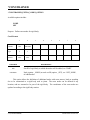
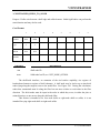
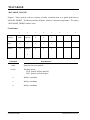
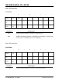
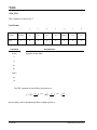
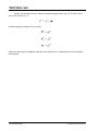
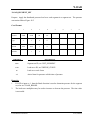
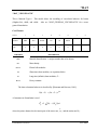
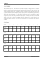
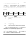
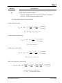
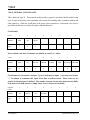
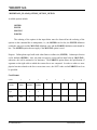
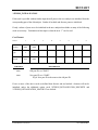
section for defining parts, and so on. Nearly all model data can be input in block form. For
example, consider the following where two nodal points with their respective coordinates and shell
elements with their part identity and nodal connectivities are defined:
$
DEFINE TWO NODES
$
$
*NODE
10101
x
y
z
10201
x
y
z
$
DEFINE TWO SHELL ELEMENTS
$
$
*ELEMENT_SHELL
10201
pid
n1
n2
10301
pid
n1
n2
n3
n3
n4
n4
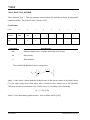
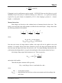
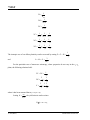
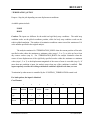
Alternatively, acceptable input could also be of the form:
$
DEFINE ONE NODE
$
$
*NODE
10101
x
y
z
$
DEFINE ONE SHELL ELEMENTS
$
I.8 (INTRODUCTION)
LS-DYNA3D Version 936
INTRODUCTION
$
*ELEMENT_SHELL
10201
pid
n1
n2
n3
$
DEFINE ONE MORE NODE
$
$
*NODE
10201
x
y
z
$
DEFINE ONE MORE SHELL ELEMENTS
$
$
*ELEMENT_SHELL
10301
pid
n1
n2
n3
n4
n4
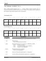
A data block begins with a keyword followed by data pertaining to the keyword. The next keyword
encountered during the reading of the block data defines the end of the block and the beginning of a
new block. A keyword must be left justified with the “*” contained in column one. A dollar sign
“$” in column one precedes a comment and causes the input line to be ignored. Data blocks are not
a requirement for LS-DYNA3D but they can be used to group nodes and elements for user
convenience. Multiple blocks can be defined with each keyword if desired as shown above. It
would be possible to put all nodal points definitions under one keyword *NODE, or to define one
*NODE keyword prior to each node definition. The entire LS-DYNA3D input is order independent
with the exception of the optional keyword, *END, which defines the end of input stream. Without
the *END termination is assumed to occur when an end-of-file is encountered during the reading.
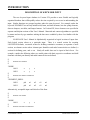
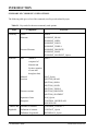
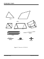
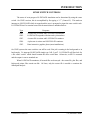
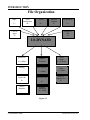
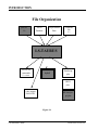
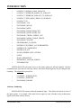
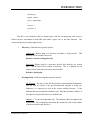
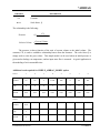
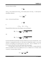
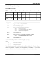
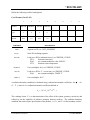
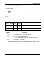
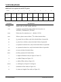
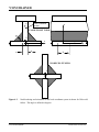
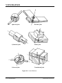
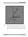
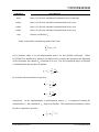
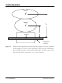
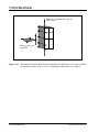
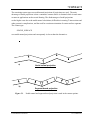
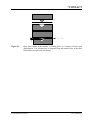
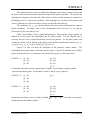
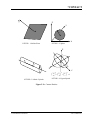
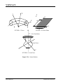
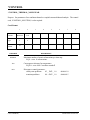
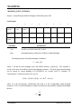
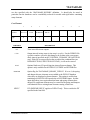
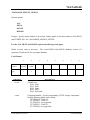
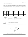
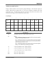
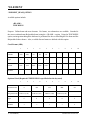
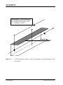
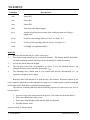
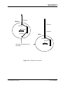
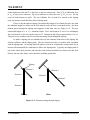
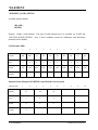
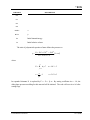
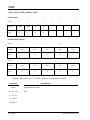
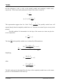
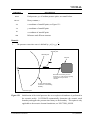
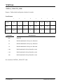
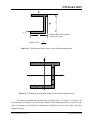
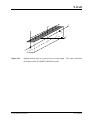
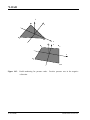
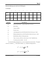
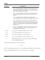
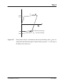
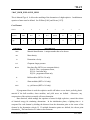
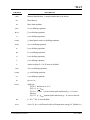
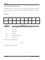
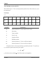
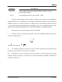
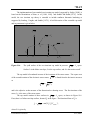
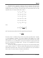
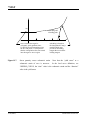
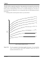
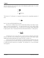
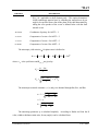
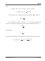
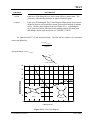
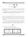
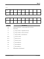
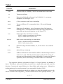
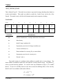
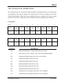
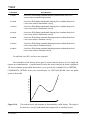
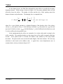
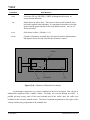
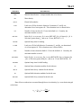
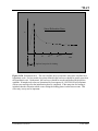
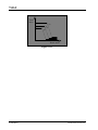
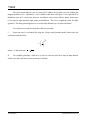
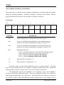
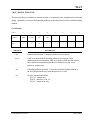
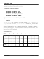
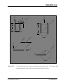
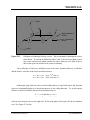
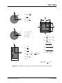
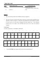
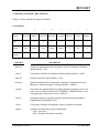
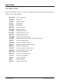
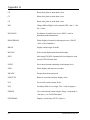
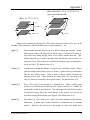
Figure I.1 attempts to show the general philosophy of the input organization and how
various entities relate to each other. In this figure the data included for the keyword, *ELEMENT,
is the element identifier, EID, the part identifier, PID, and the nodal points identifiers, the NID’s,
defining the element connectivity: N1, N2, N3, and N4. The nodal point identifiers are defined in
the *NODE section where each NID should be defined just once. A part defined with the *PART
keyword has a unique part identifier, PID, a section identifier, SID, a material or constitutive model
identifier, MID, an equation of state identifier, EOSID, and the hourglass control identifier, HGID.
The *SECTION keyword defines the section identifier, SID, where a section has an element
formation specified, a shear factor, SHRF, a numerical integration rule, NIP, and so on. The
constitutive constants are defined in the *MAT section where constitutive data is defined for all
element types including solids, beams, shells, thick shells, seat belts, springs, and dampers.
Equations of state, which are used only with certain *MAT materials for solid elements, are defined
in the *EOS section. Since many elements in LS-DYNA3D use uniformly reduced numerical
integration, zero energy deformation modes may develop. These modes are controlled numerically
LS-DYNA3D Version 936
I.9 (INTRODUCTION)
INTRODUCTION
by either an artificial stiffness or viscosity which resists the formation of these undesirable modes.
The hourglass control can optionally be user specified using the input in the *HOURGLASS
section.
During the keyword input phase where data is read, only limited checking is performed on
the data since the data must first be counted for the array allocations and then reordered.
Considerably more checking is done during the second phase where the input data is printed out.
Since LS-DYNA3D has retained the option of reading older non-keyword input files, we print out
the data into the output file D3HSP (default name) as in previous versions of LS-DYNA3D. An
attempt is made to complete the input phase before error terminating if errors are encountered in the
input. Unfortunately, this is not always possible and the code may terminate with an error message.
The user should always check either output file, D3HSP or MESSAG, for the word “Error”.
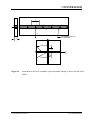
*NODE
NID
*ELEMENT
X
Y
Z
EID PID N1 N2 N3 N4
*PART
PID SID MID EOSID HGID
*SECTION_SHELL SID ELFORM SHRF NIP PROPT QR ICOMP
*MAT_ELASTIC
MID RO E PR DA DB
*EOS
EOSID
*HOURGLASS
HGID
Figure I.1 Organization of the keyword input.
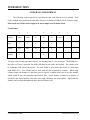
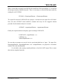
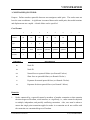
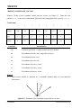
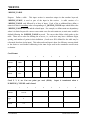
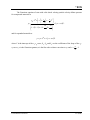
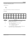
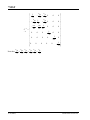
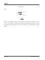
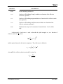
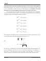
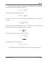
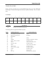
The input data following each keyword can be input in free format. In the case of free
format input the data is separated by commas, i.e.,
*NODE
10101,x ,y ,z
10201,x ,y ,z
*ELEMENT_SHELL
10201,pid,n1,n2,n3,n4
10301,pid,n1,n2,n3,n4
I.10 (INTRODUCTION)
LS-DYNA3D Version 936
INTRODUCTION
When using commas, the formats must not be violated. An I8 integer is limited to a
maximum positive value of 99999999, and larger numbers having more than eight characters are
unacceptable. The format of the input can change from free to fixed anywhere in the input file. The
input is case insensitive and keywords can be given in either upper or lower case. THE ASTERISKS
“*” PRECEDING EACH KEYWORD MUST BE IN COLUMN ONE.
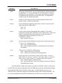
To provide a better understanding behind the keyword philosophy and how the options
work, a brief review of some of the more important keywords is given below.
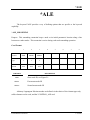
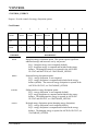
*AIRBAG
The geometric definition of airbags and the thermodynamic properties for the airbag inflator models
can be made in this section. This capability is not necessarily limited to the modeling of automotive
airbags, but it can also be used for many other applications such as tires and pneumatic dampers.
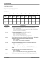
*BOUNDARY
This section applies to various methods of specifying either fixed or prescribed boundary conditions.
For compatibility with older versions of LS-DYNA3D it is still possible to specify some nodal
boundary conditions in the *NODE card section.
*CONSTRAINED
This section applies constraints within the structure between structural parts. For example, nodal
rigid bodies, rivets, spot welds, linear constraints, tying a shell edge to a shell edge with failure,
merging rigid bodies, adding extra nodes to rigid bodies and defining rigid body joints are all options
in this section.
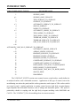
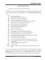
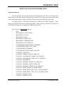
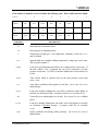
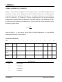
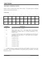
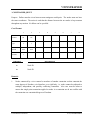
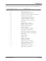
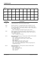
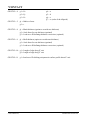
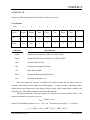
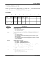
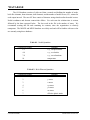
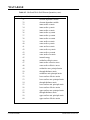
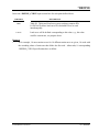
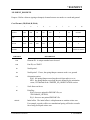
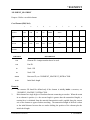
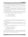
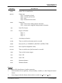
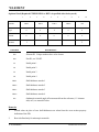
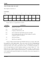
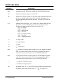
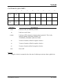
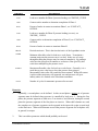
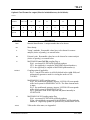
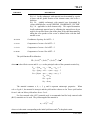
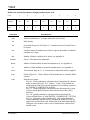
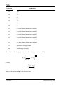
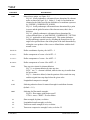
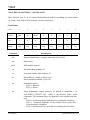
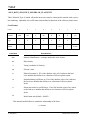
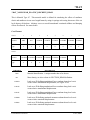
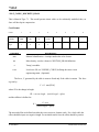
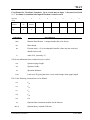
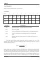
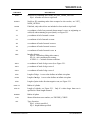
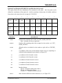
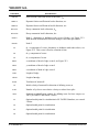
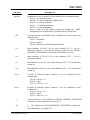
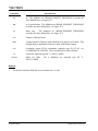
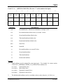
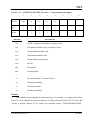
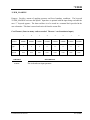
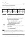
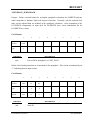
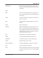
*CONTACT
This section is divided in to three main sections. The *CONTACT section allows the user to define
many different contact types. These contact options are primarily for treating contact of deformable
to deformable bodies, single surface contact in deformable bodies, deformable body to rigid body
contact, and tying deformable structures with an option to release the tie base on plastic strain. The
surface definition for contact is made up of segments on the shell or solid element surfaces. The
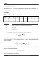
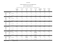
keyword options and the corresponding numbers in previous code versions are:
LS-DYNA3D Version 936
I.11 (INTRODUCTION)
INTRODUCTION
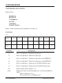
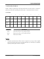
STRUCTURED INPUT TYPE ID
KEYWORD NAME
1
SLIDING_ONLY
p1
SLIDING_ONLY_PENALTY
2
TIED_SURFACE_TO_SURFACE
3
SURFACE_TO_SURFACE
a3
AUTOMATIC_SURFACE_TO_SURFACE
4
SINGLE_SURFACE
5
NODES_TO_SURFACE
a5
AUTOMATIC_NODES_TO_SURFACE
6
TIED_NODES_TO_SURFACE
7
TIED_SHELL_EDGE_TO_SURFACE
8
TIEBREAK_NODES_TO_SURFACE
9
TIEBREAK_SURFACE_TO_SURFACE
10
ONE_WAY_SURFACE_TO_SURFACE
a 10
AUTOMATIC_ONE_WAY_SURFACE_TO_SURFACE
13
AUTOMATIC_SINGLE_SURFACE
a 13
AIRBAG_SINGLE_SURFACE
14
ERODING_SURFACE_TO_SURFACE
15
ERODING_SINGLE_SURFACE
16
ERODING_NODES_TO_SURFACE
17
CONSTRAINT_SURFACE_TO_SURFACE
18
CONSTRAINT_NODES_TO_SURFACE
19
RIGID_BODY_TWO_WAY_TO_RIGID_BODY
20
RIGID_NODES_TO_RIGID_BODY
21
RIGID_BODY_ONE_WAY_TO_RIGID_BODY
22
SINGLE_EDGE
23
DRAWBEAD
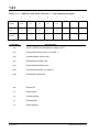
The *CONTACT_ENTITY section treats contact between a rigid surface, usually defined as
an analytical surface, and a deformable structure. Applications of this type of contact exist in the
metalforming area where the punch and die surface geometries can be input as VDA surfaces which
are treated as rigid. Another application is treating contact between rigid body occupant dummy
hyper-ellipsoids and deformable structures such as airbags and instrument panels. This option is
particularly valuable in coupling with the rigid body occupant modeling codes MADYMO and
CAL3D. The *CONTACT_1D is for modeling rebars in concrete structure.
I.12 (INTRODUCTION)
LS-DYNA3D Version 936
INTRODUCTION
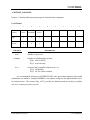
*CONTROL
Options available in the *CONTROL section allow the resetting of default global parameters such
as the hourglass type, the contact penalty scale factor, shell element formulation, numerical
damping, and termination time.
*DAMPING
Defines damping either globally or by part identifier.
*DATABASE
This keyword with a combination of options can be used for controlling the output of ASCII
databases and binary files output by LS-DYNA3D. With this keyword the frequency of writing the
various databases can be determined.
*DEFINE
This section allows the user to define curves for loadings, constitutive behaviors, etc.; boxes to limit
the geometric extent of certain inputs; local coordinate systems; vectors; and orientation vectors
specific to spring and damper elements. Items defined in this section are referenced by their
identifiers throughout the input. For example, a coordinate system identifier is sometimes used on
the *BOUNDARY cards, and load curves are used on the *AIRBAG cards.
*DEFORMABLE_TO_RIGID
This section allows the user to switch parts that are defined as deformable to rigid at the start of the
analysis. This capability provides a cost efficient method for simulating events such as rollover
events. While the vehicle is rotating the computation cost can be reduced significantly by switching
deformable parts that are not expected to deform to rigid parts. Just before the vehicle comes in
contact with ground, the analysis can be stopped and restarted with the part switched back to
deformable.
*ELEMENT
Define identifiers and connectivities for all elements which include shells, beams, solids, thick shells,
springs, dampers, seat belts, and concentrated masses in LS-DYNA3D.
LS-DYNA3D Version 936
I.13 (INTRODUCTION)
INTRODUCTION
*EOS
This section reads the equations of state parameters. The equation of state identifier, EOSID, points
to the equation of state identifier on the *PART card.
*HOURGLASS
Defines hourglass and bulk viscosity properties. The identifier, HGID, on the *HOURGLASS card
refers to HGID on *PART card.
*INCLUDE
To make the input file easy to maintain, this keyword allows the input file to be split into subfiles.
Each subfile can again be split into sub-subfiles and so on. This option is beneficial when the input
data deck is very large.
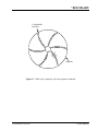
*INITIAL
Initial velocity and initial momentum for the structure can be specified in this section. The initial
velocity specification can be made by *INITIAL_VELOCITY_NODE card or *INITIAL_
VELOCITY cards. In the case of *INITIAL_VELOCITY_NODE nodal identifiers are used to
specify the velocity components for the node. Since all the nodes in the system are initialized to
zero, only the nodes with non zero velocities need to be specified. The *INITIAL_VELOCITY
card provides the capability of being able to specify velocities using the set concept or boxes.
*INTEGRATION
In this section the user defined integration rules for beam and shell elements are specified. IRID
refers to integration rule number IRID on *SECTION_BEAM and *SECTION_SHELL cards
respectively. Quadrature rules in the *SECTION_SHELL and *SECTION_BEAM cards need to
be specified as a negative number. The absolute value of the negative number refers to user defined
integration rule number. Positive rule numbers refer to the built in quadrature rules within
LS-DYNA3D.
I.14 (INTRODUCTION)
LS-DYNA3D Version 936
INTRODUCTION
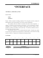
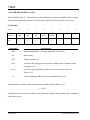
*INTERFACE
Interface definitions are used to define surfaces, nodal lines, and nodal points for which the
displacement and velocity time histories are saved at some user specified frequency. This data may
then used in subsequent analyses as an interface ID in the *INTERFACE_LINKING_DISCRETE_
NODE as master nodes, in *INTERFACE_LINKING_SEGMENT as master segments and in
*INTERFACE_LINKING_EDGE as the master edge for a series of nodes. This capability is
especially useful for studying the detailed response of a small member in a large structure. For the
first analysis, the member of interest need only be discretized sufficiently that the displacements and
velocities on its boundaries are reasonably accurate. After the first analysis is completed, the
member can be finely discretized in the region bounded by the interfaces. Finally, the second
analysis is performed to obtain highly detailed information in the local region of interest. When
beginning the first analysis, specify a name for the interface segment file using the Z=parameter on
the LS-DYNA3D execution line. When starting the second analysis, the name of the interface
segment file created in the first run should be specified using the L=parameter on the LS-DYNA3D
command line. Following the above procedure, multiple levels of sub-modeling are easily
accommodated. The interface file may contain a multitude of interface definitions so that a single
run of a full model can provide enough interface data for many component analyses. The interface
feature represents a powerful extension of LS-DYNA3D’s analysis capabilities.
*KEYWORD
Flags LS-DYNA3D that the input deck is a keyword deck. To have an effect this must be the very
first card in the input deck. Alternatively, by typing “keyword” on the execute line, keyword input
formats are assumed and the “*KEYWORD” is not required. If a number is specified on this card
after the word KEYWORD it defines the memory size to used in words. The memory size can also
be set on the command line.
*LOAD
This section provides various methods of loading the structure with concentrated point loads,
distributed pressures, body force loads, and a variety of thermal loadings.
LS-DYNA3D Version 936
I.15 (INTRODUCTION)
INTRODUCTION
*MAT
This section allows the definition of constitutive constants for all material models available in
LS-DYNA3D including springs, dampers, and seat belts. The material identifier, MID, points to the
MID on the *PART card.
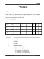
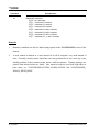
*NODE
Define nodal point identifiers and their coordinates.
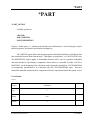
*PART
This keyword serves two purposes.
1. Relates part ID to *SECTION, *MATERIAL, *EOS and *HOURGLASS sections.
2. Optionally, in the case of a rigid material, rigid body inertia properties and initial conditions can
be specified. Deformable material repositioning data can also be specified in this section if the
reposition option is invoked on the *PART card, i.e., *PART_REPOSITION.
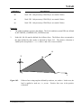
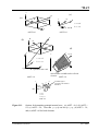
*RIGIDWALL
Rigid wall definitions have been divided into two separate sections, _PLANAR and
_GEOMETRIC. Planar walls can be either stationary or moving in translational motion with mass
and initial velocity. The planar wall can be either finite or infinite. Geometric walls can be planar as
well as have the geometric shapes such as rectangular prism, cylindrical prism and sphere. By
default, these walls are stationary unless the option MOTION is invoked for either prescribed
translational velocity or displacement. Unlike the planar walls, the motion of the geometric wall is
governed by a load curve. Multiple geometric walls can be defined to model combinations of
geometric shapes available. For example, a wall defined with the _CYLINDER option can be
combined with two walls defined with the _SPHERICAL option to model hemispherical surface
caps on the two ends of a cylinder. Contact entities are also analytical surfaces but have the
significant advantage that the motion can be influenced by the contact to other bodies, or prescribed
with six full degrees-of-freedom.
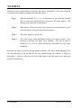
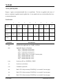
*SET
A concept of grouping nodes, elements, materials, etc., in sets is employed throughout the
LS-DYNA3D input deck. Sets of data entities can be used for output. So-called slave nodes used
I.16 (INTRODUCTION)
LS-DYNA3D Version 936
INTRODUCTION
in contact definitions, slaves segment sets, master segment sets, pressure segment sets and so on can
also be defined. The keyword, *SET, can be defined in two ways:
1. Option _LIST requires a list of entities, eight entities per card, and define as many cards as
needed to define all the entities.
2. Option _COLUMN, where applicable, requires an input of one entity per line along with up to
four attribute values which are needed to specify, for example, failure criterion input that is
needed for *CONTACT_CONSTRAINT_NODES_TO_SURFACE .
*TITLE
In this section a title for the analysis is defined.
*USER_INTERFACE
This section provides a method to provide user control of some aspects of the contact algorithms
including friction coefficients via user defined subroutines.
RESTART
This section of the input is intended to allow the user to restart the simulation by providing a restart
file and optionally a restart input defining changes to the model such as deleting contacts, materials,
elements, switching materials from rigid to deformable, deformable to rigid ,etc.
*RIGID_DEFORMABLE
This section switches rigid parts back to deformable in a restart to continue the event of a vehicle
impacting the ground which may have been modeled with a rigid wall.
*STRESS_INITIALIZATION
This is an option available for restart runs. In some cases there may be a need for the user to add
contacts, elements, etc., which are not available options for standard restart runs. A full input
containing the additions is needed if this option is invoked upon restart.
LS-DYNA3D Version 936
I.17 (INTRODUCTION)
INTRODUCTION
SUMMARY OF COMMONLY USED OPTIONS
The following table gives a list of the commonly used keywords related by topic.
Table I.1. Keywords for the most commonly used options.
Topic
Geometry
Component
Nodes
Elements
Discrete Elements
Materials
Part
Contacts and
Rigidwalls
Defaults for contacts
Definition of contacts
Definition of rigidwalls
Keyword
*NODE
*ELEMENT_BEAM
*ELEMENT_SHELL
*ELEMENT_SOLID
*ELEMENT_TSHELL
*ELEMENT_DISCRETE
*ELEMENT_MASS
*ELEMENT_SEATBELT_Option
(which is
*PART
composed of
Material and
Section, equation
of state and
hourglass data)
Material
*MAT_Option
Sections
*SECTION_BEAM
*SECTION_SHELL
*SECTION_SOLID
*SECTION_TSHELL
Discrete sections
*SECTION_DISCRETE
*SECTION_SEATBELT
Equation of state
*EOS_Option
Hourglass
*CONTROL_HOURGLASS
*HOURGLASS
I.18 (INTRODUCTION)
*CONTROL_CONTACT
*CONTACT_Option
*RIGIDWALL_Option
LS-DYNA3D Version 936
INTRODUCTION
Table I.1. (continued) Keywords for the most commonly used options.
Topic
Component
Boundary
Restraints
Conditions &
Loadings
Gravity (body) load
Point load
Pressure load
Thermal load
Load curves
Constraints
and spot
welds
Constrained nodes
Welds
Rivet
Output
Control
Termination
Keyword
*NODE
*BOUNDARY_SPC_Option
*LOAD_BODY_Option
*LOAD_NODE_Option
*LOAD_SEGMENT_Option
*LOAD_SHELL_Option
*LOAD_THERMAL_Option
*DEFINE_CURVE
*CONSTRAINED_NODE_SET
*CONSTRAINED_GENERALIZED_WELD_
Option
*CONSTRAINED_SPOT_WELD
*CONSTRAINED_RIVET
Defaults
ASCII time history files
Binary plot, time history and
restart files
Items in time history blocks
Nodes for nodal reaction
output
*CONTROL_OUTPUT
*DATABASE_Option
*DATABASE_BINARY_Option
Termination time
Termination cycle
CPU termination
Degree of freedom
*CONTROL_TERMINATION
*CONTROL_TERMINATION
*CONTROL_CPU
*TERMINATION_NODE
LS-DYNA3D Version 936
*DATABASE_HISTORY_Option
*DATABASE_NODAL_FORCE_GROUP
I.19 (INTRODUCTION)
INTRODUCTION
MATERIAL MODELS
Some of the material models presently implemented are:
•
•
•
•
•
•
•
•
•
•
•
•
•
•
•
•
•
•
•
•
•
•
•
•
•
•
•
•
•
•
•
elastic,
orthotropic elastic,
kinematic/isotropic plasticity [Krieg and Key 1976],
thermoelastoplastic [Hallquist 1979],
soil and crushable/non-crushable foam [Key 1974],
linear viscoelastic [Key 1974],
Blatz-Ko rubber [Key 1974],
high explosive burn,
hydrodynamic without deviatoric stresses,
elastoplastic hydrodynamic,
temperature dependent elastoplastic [Steinberg and Guinan 1978],
isotropic elastoplastic,
isotropic elastoplastic with failure,
soil and crushable foam with failure,
Johnson/Cook plasticity model [Johnson and Cook 1983],
pseudo TENSOR geological model [Sackett 1987],
elastoplastic with fracture,
power law isotropic plasticity,
strain rate dependent plasticity,
rigid,
thermal orthotropic,
composite damage model [Chang and Chang 1987a 1987b],
thermal orthotropic with 12 curves,
piecewise linear isotropic plasticity,
inviscid, two invariant geologic cap [Sandler and Rubin 1979, Simo et al, 1988a
1988b],
orthotropic crushable model,
Mooney-Rivlin rubber,
resultant plasticity,
force limited resultant formulation,
closed form update shell plasticity,
Frazer-Nash rubber model,
I.20 (INTRODUCTION)
LS-DYNA3D Version 936
INTRODUCTION
•
•
•
•
•
•
•
•
•
laminated glass model,
fabric,
unified creep plasticity,
temperature and rate dependent plasticity,
elastic with viscosity,
anisotropic plasticity,
user defined,
crushable cellular foams (Neilsen, Morgan, and Krieg 1987),
urethane foam model with hystersis (1992),
and some more foam and rubber models, as well as many materials models for springs and dampers.
The hydrodynamic material models determine only the deviatoric stresses. Pressure is determined
by one of ten equations of state including:
•
•
•
•
•
•
•
•
•
•
linear polynomial [Woodruff 1973],
JWL high explosive [Dobratz 1981],
Sack “Tuesday” high explosive [Woodruff 1973],
Gruneisen [Woodruff 1973],
ratio of polynomials [Woodruff 1973],
linear polynomial with energy deposition,
ignition and growth of reaction in HE [Lee and Tarver 1980, Cochran and Chan 1979],
tabulated compaction,
tabulated,
TENSOR pore collapse [Burton et. al. 1982].
The ignition and growth EOS was adapted from KOVEC [Woodruff 1973]; the other
subroutines, programmed by the authors, are based in part on the cited references and are nearly
100 percent vectorized. The forms of the first five equations of state are also given in the KOVEC
user’s manual and are retained in this manual. The high explosive programmed burn model is
described by Giroux [Simo et al. 1988].
The orthotropic elastic and the rubber material subroutines use Green-St. Venant strains to
compute second Piola-Kirchhoff stresses, which transform to Cauchy stresses. The Jaumann stress
rate formulation is used with all other materials with the exception of one plasticity model which
uses the Green-Naghdi rate.
LS-DYNA3D Version 936
I.21 (INTRODUCTION)
INTRODUCTION
SPATIAL DISCRETIZATION
The elements shown in Figure I.2 are presently available. Currently springs, dampers,
beams, membranes, shells, bricks, brick shells and seatbelt elements are included.
The first shell element in DYNA3D was that of Hughes and Liu [Hughes and Liu 1981a,
1981b, 1981c], implemented as described in [Hallquist et al. 1985, Hallquist and Benson 1986].
This element [designated as HL] was selected from among a substantial body of shell element
literature because the element formulation has several desirable qualities:
•
It is incrementally objective (rigid body rotations do not generate strains), allowing for
the treatment of finite strains that occur in many practical applications;
•
It is compatible with brick elements, because the element is based on a degenerated brick
element formulation. This compatibility allows many of the efficient and effective
techniques developed for the DYNA3D brick elements to be used with this shell element;
•
It includes finite transverse shear strains;
•
A through-the-thickness thinning option (see [Hughes and Carnoy 1981]) is also
available.
All shells in our current LS-DYNA3D code must satisfy these desirable traits to at least some extent
to be useful in metalforming and crash simulations.
The major disadvantage of the HL element turned out to be cost related and, for this reason,
within a year of its implementation we looked at the Belytschko-Tsay [BT] shell [Belytschko and
Tsay 1981 1983 1984] as a more cost effective, but possibly less accurate alternative. In the BT
shell the geometry of the shell is assumed to be perfectly flat, the local coordinate system originates
at the first node of the connectivity, and the co-rotational stress update does not use the costly
Jaumann stress rotation. With these and other simplifications, a very cost effective shell was derived
which today has become perhaps the most widely used shell elements in both metalforming and
crash applications. Results generated by the BT shell usually compare favorably with those of the
more costly HL shell. Triangular shell elements are implemented, based on work by Belytschko and
co-workers [Belytschko and Marchertas 1974, Bazeley et al. 1965, Belytschko et al. 1984], and are
frequently used since collapsed quadrilateral shell elements tend to lock and give very bad results.
LS-DYNA3D automatically treats collapsed quadrilateral shell elements as C0 triangular elements
Since the Belytschko-Tsay element is based on a perfectly flat geometry, warpage is not
considered. Although this generally poses no major difficulties and provides for an efficient
element, incorrect results in the twisted beam problem and similar situations are obtained where the
nodal points of the elements used in the discretization are not coplanar. The Hughes-Liu shell
I.22 (INTRODUCTION)
LS-DYNA3D Version 936
INTRODUCTION
element considers non-planar geometries and gives good results on the twisted beam. The effect of
neglecting warpage in a typical application cannot be predicted beforehand and may lead to less than
accurate results, but the latter is only speculation and is difficult to verify in practice. Obviously, it
would be better to use shells that consider warpage if the added costs are reasonable and if this
unknown effect is eliminated. A new shell has been recently published by Belytschko, Wong, and
Chiang [Belytschko, Wong, and Chang 1989, 1992] in which inexpensive modifications were
proposed to include the warping stiffness in the Belytschko-Tsay shell. An improved transverse
shear treatment also allows the element to pass the Kirchhoff patch test. This element is now
available in LS-DYNA3D. Also, two shell elements which use full integration are available in
LS-DYNA3D, but are rather expensive.
Three-dimensional plane stress constitutive subroutines are implemented for the shell
elements which iteratively updates the stress tensor such that the stress component normal to the
shell midsurface is zero. An iterative update is necessary to accurately determine the normal strain
component which is necessary to predict thinning. One constitutive evaluation is made for each
integration point through the shell thickness.
Zero energy modes in the shell and solid elements are controlled by either an hourglass
viscosity or stiffness. Eight node solid-shell elements are implemented and have been found to
perform well in many applications. All elements are nearly 100% vectorized. All element classes
can be included as parts of a rigid body. The rigid body formulation is documented in [Benson and
Hallquist 1986]. Rigid body point nodes, as well as concentrated masses, springs and dashpots can
be added to this rigid body.
Membrane elements can be either defined directly as shell elements with a membrane
formulation option or as shell elements with only one point for through thickness integration. The
latter choice includes transverse shear stiffness and may be inappropriate. For airbag material a
special fully integrated three and four node membrane element is available.
Two different beam types are available: a stress resultant beam and a beam with cross
section integration at one point along the axis. The cross section integration allows for a more
general definition of arbitrarily shaped cross sections taking into account material nonlinearities.
Spring and damper elements can be translational or rotational. Many behavior options can
be defined, e.g., arbitrary nonlinear behavior including locking and separation.
Solid elements in LS-DYNA3D may be defined using from 4 to 8 nodes. The standard
elements are based on linear shape functions and use one point integration and hourglass control. A
selective-reduced integrated (called fully integrated) 8 node solid element is available for situations
when the hourglass control fails. Also, two additional solid elements, a 4 noded tetrahedron and an
8 noded hexahedron, with nodal rotational degrees of freedom, are implemented based on the idea
of Allman [1984] to replace the nodal midside translational degrees of freedom of the elements with
LS-DYNA3D Version 936
I.23 (INTRODUCTION)
INTRODUCTION
quadratic shape functions by corresponding nodal rotations at the corner nodes. The latter
elements, which do not need hourglass control, require many numerical operations compared to the
hourglass controlled elements and should be used at places where the hourglass elements fail.
However, it is well known that the elements using more than one point integration are more
sensitive to large distortions than one point integrated elements.
The brick shell or solid shell element is a shell element with only nodal translations for the
eight nodes. The assumptions of shell theory are included in a non-standard fashion. It also uses
hourglass control or selective-reduced integration. This element can be used in place of any four
node shell element. It is favorably used for shell-brick transitions, as no additional constraint
conditions are necessary. However, care has to be taken to know in which direction the shell
assumptions are made; therefore, the numbering of the element is important.
Seatbelt elements can be separately defined to model seatbelt actions combined with dummy
models. Separate definitions of seatbelts, which are one-dimensional elements, with accelerometers,
sensors, pretensioners, retractors, and sliprings are possible. The actions of the various seatbelt
definitions can also be arbitrarily combined.
I.24 (INTRODUCTION)
LS-DYNA3D Version 936
INTRODUCTION
SLIDING INTERFACES
The three-dimensional contact-impact algorithm was originally an extension of the NIKE2D
[Hallquist 1979] two-dimensional algorithm. As currently implemented, one surface of the interface
is identified as a master surface and the other as a slave. Each surface is defined by a set of three or
four node quadrilateral segments, called master and slave segments, on which the nodes of the slave
and master surfaces, respectively, must slide. In general, an input for the contact-impact algorithm
requires that a list of master and slave segments be defined. For the single surface algorithm only the
slave surface is defined and each node in the surface is checked each time step to ensure that it does
not penetrate through the surface. Internal logic [Hallquist 1977, Hallquist et al. 1985] identifies a
master segment for each slave node and a slave segment for each master node and updates this
information every time step as the slave and master nodes slide along their respective surfaces. It
must be noted that for general automatic definitions only parts/materials or three-dimensional boxes
have to be given. Then the possible contacting outer surfaces are identified by the internal logic in
LS-DYNA3D. More than 20 types of interfaces can presently be defined including:
sliding only for fluid/structure or gas/structure interfaces,
tied,
sliding, impact, friction,
single surface contact,
discrete nodes impacting surface,
discrete nodes tied to surface,
shell edge tied to shell surface,
nodes spot welded to surface,
tiebreak interface,
one way treatment of sliding, impact, friction,
box/material limited automatic contact for shells,
automatic contact for shells (no additional input required),
automatic single surface with beams and arbitrary orientations,
surface to surface eroding contact,
node to surface eroding contact,
single surface eroding contact,
surface to surface symmetric constraint method [Taylor and Flanagan 1989],
node to surface constraint method [Taylor and Flanagan 1989],
rigid body to rigid body contact with arbitrary force/deflection curve,
rigid nodes to rigid body contact with arbitrary force/deflection curve,
LS-DYNA3D Version 936
I.25 (INTRODUCTION)
INTRODUCTION
edge-to-edge,
draw beads.
Interface friction can be used with most interface types. The tied and sliding only interface
options are similar to the two-dimensional algorithm used in LS-DYNA2D [Hallquist 1976, 1978,
1980]. Unlike the general option, the tied treatments are not symmetric; therefore, the surface
which is more coarsely zoned should be chosen as the master surface. When using the one-way
slide surface with rigid materials, the rigid material should be chosen as the master surface.
For geometric contact entities, contact has to be separately defined. It must be noted that
for the contact of a rigid body with a flexible body, either the sliding interface definitions as
explained above or the geometric contact entity contact can be used. Currently, the geometric
contact entity definition is recommended for metalforming problems due to high accuracy and
computational efficiency.
I.26 (INTRODUCTION)
LS-DYNA3D Version 936
INTRODUCTION
INTERFACE DEFINITIONS FOR COMPONENT ANALYSIS
Interface definitions for component analyses are used to define surfaces, nodal lines, or
nodal points for which the displacement and velocity time histories are saved at some user specified
frequency. This data may then used in subsequent analyses as master surfaces of type
TIED_SURFACE_TO_SURFACE sliding interfaces of Section 31, as master lines in the tie
breaking shell definitions, or as the controlling nodes for determining the motion of single nodal
points. This capability is especially useful for studying the detailed response of a small member in a
large structure. For the first analysis, the member of interest need only be discretized sufficiently
that the displacements and velocities on its boundaries are reasonably accurate. After the first
analysis is completed, the member can be finely discretized and interfaces defined to correspond
with the first analysis. Finally, the second analysis is performed to obtain highly detailed information
in the local region of interest.
When starting the analysis, specify a name for the interface segment file using the
Z = parameter on the LS-DYNA3D command line. When starting the second analysis, the name of
the interface segment file (created in the first run) should be specified using the L = parameter on
the LS-DYNA3D command line.
Following the above procedure, multiple levels of sub-modeling are easily accommodated.
The interface file may contain a multitude of interface definitions so that a single run of a full model
can provide enough interface data for many component analyses. The interface feature represents a
powerful extension of LS-DYNA3D’s analysis capability.
LS-DYNA3D Version 936
I.27 (INTRODUCTION)
INTRODUCTION
shells
solids
trusses
beams
springs
lumped masses
dampers
Figure I.2. Elements in LS-DYNA3D.
I.28 (INTRODUCTION)
LS-DYNA3D Version 936
INTRODUCTION
CAPACITY
Storage allocation is dynamic. The only limit that exists on the number of boundary
condition cards, number of material cards, number of pressure cards, etc., is the capacity of the
computer. Typical LS-DYNA3D calculations may have 10,000 to 200,000 elements. Memory
allocation is dynamic and can be controlled during execution.
LS-DYNA3D Version 936
I.29 (INTRODUCTION)
INTRODUCTION
CODE ORGANIZATION
LS-DYNA3D consists of one source that compiles under FORTRAN compilers on most
UNIX workstations and supercomputers. The programming follows the FORTRAN 77 standard
with some parts programmed in C. LS-DYNA3D has eight segments in the main code. They are:
•
•
•
•
•
•
•
•
input,
restart,
initialization,
solution,
interactive real time graphics,
rezoning,
remapping,
thermal.
Parallel versions of LS-DYNA3D for shared memory are supported for the SGI and CRAY
computers, and a distributed memory version of LS-DYNA3D has been ported to a subset of the
commercially available MPP machines incuding the CRAY-T3D, IBM SP1/SP2, and the INTEL
PARAGON.
I.30 (INTRODUCTION)
LS-DYNA3D Version 936
INTRODUCTION
SENSE SWITCH CONTROLS
The status of an in-progress LS-DYNA3D simulation can be determined by using the sense
switch. On UNIX versions, this is accomplished by first typing a “^C” (Control-C). This sends an
interrupt to LS-DYNA3D which is trapped and the user is prompted to input the sense switch code.
LS-DYNA3D has five terminal sense switch controls that are tabulated below:
Type
SW1.
SW2.
SW3.
SW4.
SW5.
Response
A restart file is written and LS-DYNA3D terminates.
LS-DYNA3D responds with time and cycle numbers.
A restart file is written and LS-DYNA3D continues.
A plot state is written and LS-DYNA3D continues.
Enter interactive graphics phase (most installations).
On UNIX systems the sense switches can still be used if the job is running in the background or in
batch mode. To interrupt LS-DYNA3D simply type “kill -2 psid”. LS-DYNA3D will first look for
a file called “switch” which should contain the sense switch data. Otherwise, an SW2 is assumed
and the output is sent to standard out.
When LS-DYNA3D terminates, all scratch files are destroyed: the restart file, plot files, and
high-speed printer files remain on disk. Of these, only the restart file is needed to continue the
interrupted analysis.
LS-DYNA3D Version 936
I.31 (INTRODUCTION)
INTRODUCTION
PRECISION
The explicit time integration algorithms used in LS-DYNA3D are in general much less
sensitive to machine precision than other finite element solution methods. Consequently, double
precision is not used. The benefits of this are greatly improved utilization of memory and disk.
When problems have been found we have usually been able to overcome them by reorganizing the
algorithm or by converting to double precision locally in the subroutine where the problem occurs.
A few of the known problems include: (32-bit computers only!):
•
•
Round-off errors can cause difficulties with extremely small deflection problems.
(Maximum vibration amplitudes are <10-6 times nodal coordinates).
Workaround: Increase the load.
Buckling problems, which are very sensitive to small imperfections.
However, the users of LS-DYNA3D have to be aware of potential problems.
A major reorganization of LS-DYNA3D has led to a version using double precision
throughout the full program. As memory and disk space of the computers is less of a problem, we
prefer to provide this version for all machines. It also allows LS-DYNA3D to take advantage of the
64-bit technology offered by some computer manufacturers.
I.32 (INTRODUCTION)
LS-DYNA3D Version 936
INTRODUCTION
EXECUTION SYNTAX
The interactive execution line for LS-DYNA3D is as follows:
LS-DYNA3D I=inf O=otf G=ptf D=dpf F=thf U=xtf T=tpf A=rrd M=sif J=jif S=iff Z=isf1
L=isf2 B=rlf W=root E=efl X=scl C=cpu K=kill V=vda Y=c3d KEYWORD MEMORY=nwds
where
inf
otf
ptf
dpf
thf
xtf
tpf
rrd
sif
jif
iff
isf1
isf2
rlf
efl
root
scl
cpu
kill
=
=
=
=
input file (user specified),
high speed printer file (default=D3HSP),
binary plot file for graphics (default=D3PLOT),
dump file for restarting (default=D3DUMP),
=
=
=
=
=
=
=
=
=
=
=
=
=
binary plot file for time histories of selected data (default=D3THDT),
binary plot file for time extra data (default-XTFILE)
optional temperature file (TOPAZ3D plotfile),
running restart dump file (default=RUNRSF),
stress initialization file (user specified),
optional JOY interface file,
interface force file (user specified),
interface segment save file to be created (user specified),
existing interface segment save file to be used (user specified),
binary plot file for dynamic relaxation (default=D3DRFL),
echo file containing optional input echo with or without node/element data,
root file name for general print option,
scale factor for binary file sizes (default=7),
= cpu limit in seconds, applies to total calculation not just cpu from a restart,
= if LS-DYNA3D encounters this file name it will terminate with a restart file
(default=D3KIL),
vda = VDA/IGES database for geometrical surfaces,
c3d = CAL3D input file,
nwds = Number of words to be allocated. On engineering workstations a word is usually
32bits.
In order to avoid undesirable results, each LS-DYNA3D run should be performed in a separate
directory. Also, files should be removed or renamed to avoid confusion. By including
KEYWORD anywhere on the execute line or instead if *KEYWORD is the first card in the input
file, the keyword formats are expected; otherwise, the older structured input file will be expected.
LS-DYNA3D Version 936
I.33 (INTRODUCTION)
INTRODUCTION
File Organization
input
stress
initialization
M=
I=
restart
R=
CAL3D
input
Y=
interface
segment
1L==
vda geometry
V=
TOPAZ3D
file
T=
LS-DYNA3D
printer file
graphics
O = d3hsp
G=d3plot
messag
time histories
f = d3thdt
input echo
interface force
E=
S=
ASCII
Database
dynamic
relaxation
B = d3drfl
restart
dump
D = d3dump
running restart
dump
A = runrsf
interface
segment save
Z=
Figure I.3
I.34 (INTRODUCTION)
LS-DYNA3D Version 936
INTRODUCTION
If the word MEMORY is found anywhere on the execution line and if it is not set via (=nwds)
LS-DYNA3D will give the default size of memory, request, and then read in the desired memory
size. This option is necessary if the default value is insufficient memory and termination occurs as a
result. Occasionally, the default value is too large for execution and this option can be used to
lower the default size.
File names must be unique. The interface force file is created only if it is specified on the
execution line (S=iff). On large problems the default file sizes may not be large enough for a single
file to hold either a restart dump or a plot state. Then the file size may be increased by specifying
the file size on the execute line using X=scl. The default file size holds seven times one-million octal
word (262144) or 1835008 words. If the core required by LS-DYNA3D requires more space, it is
recommended that the scl be increased appropriately. Using C=cpu defines the maximum cpu usage
allowed that if exceeded will cause LS-DYNA3D to terminate with a restart file. During a restart,
cpu should be set to the total cpu used up to the current restart plus whatever amount of additional
time is wanted.
When restarting from a dump file, the execution line becomes
LS-DYNA3D I=inf O=otf G=ptf D=dpf R=rtf F=thf U=xtf T=tpf A=rrd J=jif S=iff Z=isf1
L=isf2 B=rlf W=root E=efl X=scl C=cpu K=kill Q=option KEYWORD MEMORY=nwds
where
rtf = restart filename.
If the data from the last run is to be remapped onto a new mesh, then specify: Q=remap. The
remap file is the dump file from which the remapping data are taken. The remap option is available
for brick elements only. File name dropouts are permitted; for example, the execution lines are
acceptable.
LS-DYNA3D I=inf
LS-DYNA3D R=rtf
Default names for the output file, binary plot files, and the dump file are D3HSP, D3PLOT,
D3THDT, and D3DUMP, respectively.
For an analysis using interface segments the execution line in the first analysis is given by:
LS-DYNA3D I=inf Z=isf1
LS-DYNA3D Version 936
I.35 (INTRODUCTION)
INTRODUCTION
and in the second by:
LS-DYNA3D I=inf L=isf1
Batch execution in some installations (e.g., GM) is controlled by file NAMES on unit 88.
NAMES is a 2 line file in which the second line is blank. The first line of NAMES contains the
execution line:
I=inf
if this is the initial run. For a restart the execution line becomes:
I=inf R=rtf
Remark: No stress initialization is possible at restart. Also the VDA files and the CAL3D files
cannot be changed.
I.36 (INTRODUCTION)
LS-DYNA3D Version 936
INTRODUCTION
RESTART ANALYSIS
The LS-DYNA3D restart capability allows analyses to be broken down into stages. After the
completion of each stage in the calculation a “restart dump” is written that contains all information
necessary to continue the analysis. The size of this “dump” file is roughly the same size as the
memory required for the calculation. Results can be checked at each stage by post-processing the
output databases in the normal way, so the chance of wasting computer time on incorrect analyses is
reduced. The restart capability is frequently used to modify models by deleting excessively distorted
elements, materials that are no longer important, and contact surfaces that are no longer needed.
Output frequencies of the various databases can also be altered. Often, these simple modifications
permit the calculation to continue on to a successful completion. Restarting can also help to
diagnose why a model is giving problems. By restarting from a dump that is written before the
occurrence of a numerical problem and obtaining output at more frequent intervals, it is often
possible to identify where the first symptoms appear and what aspect of the model is causing them.
The format of the restart input file is described in this manual. If, for example, the user
wishes to restart the analysis from dump state nn, contained in file D3DUMPnn, then the following
procedure is followed:
1. Create the restart input deck, if required, as described in the Restart Section of this
manual. Call this file restartinput.
2. By invoking the execution line:
LS-DYNA3D I=restartinput R=D3DUMPnn
execution begins. If no alterations to the model are made, then the execution line:
LS-DYNA3D R=D3DUMPnn
will suffice. Of course, the other output files should be assigned names if the defaults
have been changed in the original run.
The R=D3DUMPnn on the status line informs the program that this is a restart analysis.
The full deck restart option allows the user to begin a new analysis, with deformed shapes
and stresses carried forward from a previous analysis for selected materials. The new analysis can
be different from the original, e.g., more contact surfaces, different geometry (of parts which are not
carried forward), etc. Examples of applications include:
•
•
Crash analysis continued with extra contact surfaces;
Sheet metalforming continued with different tools for modeling a multi-stage forming
process.
LS-DYNA3D Version 936
I.37 (INTRODUCTION)
INTRODUCTION
Assume an analysis is run using the input file, job1.inf, and a restart dump named d3dump01
is created. A new input file job2.inf is generated and submitted as a restart with R=d3dump01 as the
dump file. The input file job2.inf contains the entire model in its original undeformed state but with
more contact surfaces, new output databases, and so on. Since this is a restart job, information
must be given to tell LS-DYNA3D which parts of the model should be initialized in the full deck
restart. When the calculation begins the restart database contained in the file d3dump01 is read, and
a new database is created to initialize the model in the input file, job2.inf. The data in file job2.inf is
read and the LS-DYNA3D proceeds through the entire input deck and initialization. At the end of
the initialization process, all the parts selected are initialized from the data saved from d3dump01.
This means that the deformed position and velocities of the nodes on the elements of each part, and
the stresses and strains in the elements (and, if the material of the part is rigid, the rigid body
properties) will be assigned.
It is assumed during this process that any initialized part has the same elements, in the same
order, with the same topology, in job1 and job2. If this is not the case, the parts cannot be
initialized. However, the parts may have different identifying numbers.
For discrete elements and seat belts, the choice is all or nothing. All discrete and belt
elements, retractors, sliprings, pretensioners and sensors must exist in both files and will be
initialized.
Materials which are not initialized will have no initial deformations or stresses. However, if
initialized and non-initialized materials have nodes in common, the nodes will be moved by the
initialized material causing a sudden strain in the non-initialized material. This effect could give rise
to sudden spikes in loading.
Points to note are:
•
Time and output intervals are continuous with job1, i.e., the time is not reset to zero.
•
Don’t try to use the restart part of the input to change anything since this will be
overwritten by the new input file.
•
Usually, the complete input file part of job2.in1 will be copied from job1.inf, with the
required alterations. We again mention that there is no need to update the nodal
coordinates since the deformed shapes of the initialized materials will be carried forward
from job1.
•
Completely new databases will be generated with the time offset.
I.38 (INTRODUCTION)
LS-DYNA3D Version 936
INTRODUCTION
VDA/IGES DATABASES
VDA surfaces are surfaces of geometric entities which are given in the form of polynomials.
The format of these surfaces is as defined by the German automobile and supplier industry in the
VDA guidelines, [VDA, 1987].
The advantage of using VDA surfaces is twofold. First, the problem of meshing the surface
of the geometric entities is avoided and, second, smooth surfaces can be achieved which are very
important in metalforming. With smooth surfaces, artificial friction introduced by standard faceted
meshes with corners and edges can be avoided. This is a big advantage in springback calculations.
A very simple and general handling of VDA surfaces is possible allowing arbitrary motion
and generation of surfaces. For a detailed description, see Appendix I.
LS-DYNA3D Version 936
I.39 (INTRODUCTION)
INTRODUCTION
MESH GENERATION
LS-DYNA3D is designed to operate with a variety of commercial pre-processing packages.
Currently, direct support is available from PATRAN1, FEMB, HYPERMESH, and MEDINA.
Several third-party translation programs are available for PATRAN and IDEAS.
Alternately, the pre-processor LS-INGRID [LSTC Report 1019] is available from LSTC and
is specialized to LS-DYNA3D. Some of the capabilities available in LS-INGRID are:
Complete support for all control parameters, loads and material types,
Mass property calculations,
Importing models from other sources (PATRAN, IDEAS, IGES and NASTRAN formats),
Interactive viewing and graphical inspection of boundary conditions, etc.,
Model editing,
General purpose mesh generation,
Importing LS-DYNA3D and DYNA3D models in a variety of older formats,
Complex surface treatment including NURB surfaces,
Parametric modeling.
Capabilities specialized to automotive applications:
Airbag folding and inspection,
Occupant positioning,
Seat belt positioning (both beam and shells),
Merging of occupants, airbags and belts with car models.
1
PATRAN is a trademark of PDA Engineering, HYPERMESH is a trademark of Altair Engineering, FEMB is a trademark of
Engineering Technology Associates, IDEAS is a trademark of Structural Dynamics Research Corporation.
I.40 (INTRODUCTION)
LS-DYNA3D Version 936
INTRODUCTION
TAURUS POST-PROCESSING
LS-TAURUS [Brown and Hallquist 1984] processes output from LS-DYNA3D.
LS-TAURUS reads the binary plot-files generated by LS-DYNA3D and plots contours, fringes,
time histories, and deformed shapes. Color contours and fringes of a large number of quantities may
be interactively plotted on meshes consisting of plate, shell, and solid type elements. LS-TAURUS
can compute a variety of strain measures, reaction forces along constrained boundaries, and
momenta. LS-TAURUS is operational on the CRAY, VAX, SUN, APOLLO, IBM RS6000, SGI,
STARDENT, HP and MIPS computers. Interfaces from LS-TAURUS to other commercial postprocessors are available.
LS-DYNA3D generates three binary databases. One contains information for complete
states at infrequent intervals; 50 to 100 states of this sort is typical in a LS-DYNA3D calculation.
The second contains information for a subset of nodes and elements at frequent intervals; 1000 to
10,000 states is typical. The third contains interface data for contact surfaces.
Because of the difficulty in handling one large file, an alternative method for obtaining
printed output is also available. Many ASCII databases are created at the user’s option containing
such information as cross-sectional forces, rigidwall forces, nodal point data, element integration
point data, global data like total internal and kinetic energy, material energies, nodal interface forces,
resultant interface forces, single point constraint forces, as well as files that are compatible with
MOVIE.BYU and the Cray Research developed post-processor, MPGS. A SMUG animator
database and a NASTRAN BDF file is written for users at General Motors. Each ASCII database is
written at its own unique output interval defined in the user input.
LS-DYNA3D Version 936
I.41 (INTRODUCTION)
INTRODUCTION
File Organization
plot file
ASCII
Database
G=
Experimental
Data
command
file
C=
LS-TAURUS
save file for
commands
S = tsave
hspbull
PostScript
plot
HPGL
plot
video output
PAL/NTSC
HP Laserjet
pcl plot
Figure I.4
I.42 (INTRODUCTION)
LS-DYNA3D Version 936
INTRODUCTION
EXECUTION SPEEDS
The execution speeds on the Cray-YMP for various elements in LS-DYNA3D are tabulated
below in microseconds per element cycle:
Element Type
CPU Cost
8 node solid with 1 point integration and default
hourglass control
12
as above but with Flanagan-Belytschko hourglass
control
15
constant stress and Flanagan-Belytschko hourglass
control, i.e., the Flanagan-Belytschko element
20
4 node Belytschko-Tsay shell with four thickness
integration points
11
4 node Belytschko-Tsay shell with resultant plasticity
9
BCIZ triangular shell with four thickness integration points
22
Co triangular shell with four thickness integration points
11
2 node Hughes-Liu beam with four integration points
28
2 node Belytschko-Schwer beam
5
2 node simple truss elements
3
8 node solid-shell with four through the thickness
integration points
33
These timings are very approximate and do not account for the inclusion of sliding interfaces or
complex material models. Each interface node of the sliding interfaces is roughly equivalent to onehalf zone cycle in cost. Figure I.5 illustrates the relative cost of the various shell formulations in
LS-DYNA3D.
LS-DYNA3D Version 936
I.43 (INTRODUCTION)
INTRODUCTION
20.01
30
8.84
Performance
20
1.28
1.49
YASE
BWC
CHL
2.45
1.25
1.07
1
10
0
BT
BTW
HL
CFHL
FHL
Element Type
Figure I.5.
Relative cost of the four noded shells available in LS-DYNA3D where BT is the
Belytschko-Tsay shell, BTW is the Belytschko-Tsay shell with the warping stiffness
taken from the Belytschko-Wong-Chiang, BWC, shell. The YASE shell is the
Englemann-Whirley shell. CHL denotes the Hughes-Liu shell, HL, with one point
quadrature and a co-rotational formulation. FHL is the fully integrated Hughes-Liu
shell, and the CFHL shell is its co-rotational version.
I.44 (INTRODUCTION)
LS-DYNA3D Version 936
INTRODUCTION
UNITS
The units in LS-DYNA3D must be consistent. One way of testing whether a set of units is
consistent is to check that:
1 (force unit) = 1 (mass unit) x 1 (acceleration unit)
1 (length unit)
[1 (time unit)]2
and that 1 (acceleration unit) =
Examples of sets of consistent units are:
(a)
(b)
(c)
Length unit
meter
millimeter
millimeter
Time unit
second
second
millisecond
Mass unit
kilogram
tonne
kilogram
Force unit
Newton
Newton
kiloNewton
Young’s Modulus of Steel
210.0E+09
210.0E+03
210.0
Density of Steel
7.85E+03
7.85E–09
7.85E–06
Yield stress of Mild Steel
200.0E+06
200.0
0.200
Acceleration due to gravity
9.81
9.81E+03
9.81E–03
Velocity equivalent to 30 mph
13.4
13.4E+03
13.4
LS-DYNA3D Version 936
I.45 (INTRODUCTION)
INTRODUCTION
GENERAL CARD FORMAT
The following sections specify for each keyword the cards that have to be defined. Each
card is defined in its rigid format form and is shown as a number of fields in an 80 character string.
Most cards are 8 fields with a length of 10 and a sample card is shown below.
Card Format
1
2
3
4
5
6
NSID
PSID
A1
A2
A3
SASH
I
I
F
F
F
I
Default
none
none
1.0
1.0
0
1
Remarks
1
Variable
Type
2
7
8
3
The type is the variable type and is either F, for floating point or I, for an integer. The default gives
the value set if zero is specified, the field is left blank or the card is not defined. The remarks refer
to comments at the end of the section. The card format is given above the card if it is other than
eight fields of 10. Free formats may be used with the data separated by commas. When using
comma format, the number of characters used to specify a number must not exceed the number
which would fit into the equivalent rigid format field. An I8 number is limited to a number of
99999999 and larger numbers with more than eight characters are unacceptable. Rigid and free
formats can be mixed throughout the deck but not within a card.
I.46 (INTRODUCTION)
LS-DYNA3D Version 936
INTRODUCTION
MPP/LS-DYNA3D USER INFORMATION
Supported Features
First and foremost, the only input formats currently supported are 920, 930, and keyword.
Models in any of the older formats will need to be converted to one these input formats before then
can be run with the current version of LS-DYNA3D for massively parallel processors, mpp.
The large majority of LS-DYNA3D options are available on the MPP computers. Those
that are not supported are being systematically added. Unless otherwise noted here, all options of
LS-DYNA3D version 93x are supported by MPP/LS-DYNA3D.
Here is the list of unsupported options:
•
*ALE
•
*BOUNDARY_CONVECTION
•
*BOUNDARY_CYCLIC
•
*BOUNDARY_FLUX
•
*BOUNDARY_RADIATION
•
*BOUNDARY_TEMPERATURE
•
*BOUNDARY_USA_SURFACE
•
*CONSTRAINED_RIGID_BODY_STOPPERS
•
*CONSTRAINED_SHELL_TO_SOLID
•
*CONSTRAINED_TIE-BREAK
•
*CONSTRAINED_TIED_NODES_FAILURE
•
*CONTROL_ADAPTIVE
•
*CONTACT_AIRBAG_SINGLE_SURFACE
•
*CONTACT_CONSTRAINT_NODES_TO_SURFACE
•
*CONTACT_CONSTRAINT_SURFACE_TO_SURFACE
•
*CONTACT_DRAWBEAD
•
*CONTACT_ERODING_NODES_TO_SURFACE
•
*CONTACT_ERODING_SINGLE_SURFACE
•
*CONTACT_ERODING_SURFACE_TO_SURFACE
•
*CONTACT_RIGID_NODES_TO_RIGID_BODY
•
*CONTACT_RIGID_BODY_ONE_WAY_TO_RIGID_BODY
•
*CONTACT_RIGID_BODY_TWO_WAY_TO_RIGID_BODY
•
*CONTACT_SINGLE_EDGE
•
*CONTACT_SLIDING_ONLY
LS-DYNA3D Version 936
I.47 (INTRODUCTION)
INTRODUCTION
•
•
•
•
•
•
•
•
•
•
•
•
•
•
•
•
•
•
•
•
•
•
*CONTACT_SLIDING_ONLY_PENALTY
*CONTACT_TIEBREAK_NODES_TO_SURFACE
*CONTACT_TIEBREAK_SURFACE_TO_SURFACE
*CONTACT_TIED_SHELL_EDGE_TO_SURFACE
*CONTACT_1D
*DATABASE_AVS
*DATABASE_MOVIE
*DATABASE_MPGS
*DATABASE_BEAM, BEAM_SET
*DATABASE_SOLID, SOLID_SET
*DATABASE_TSHELL, TSHELL_SET
*DATABASE_NODAL_FORCE_GROUP
*DATABASE_TRACER
*DEFORMABLE_TO_RIGID
*ELEMENT_SEATBELT_ACCELEROMETER
*INTERFACE_COMPONENT
*INTERFACE_JOY
*LOAD_SUPERPLASTIC_OPTION
*USER
*PART_REPOSITION
*RIGIDWALL_PLANAR_FORCES
*TERMINATION
MPP/LS-DYNA3D can restart; however, the restart options are still quite limited. Only the
termination time, plot interval, time step control, and restart dump frequency may be changed when
restarting. The supported keywords are:
•
•
•
*CONTROL_TERMINATION
*CONTROL_TIMESTEP
*DATABASE_BINARY
Arbitrary Numbering
MPP/LS-DYNA3D assumes arbitrarily numbered input. This affects the format of some of
the input options. For example, if the initial velocity option is used, all nodes in the problem must
appear in the initial velocity section.
I.48 (INTRODUCTION)
LS-DYNA3D Version 936
INTRODUCTION
Contact Interfaces
MPP/LS-DYNA3D uses a completely redesigned, highly parallel contact algorithm. The
contact options currently supported include:
•
•
•
•
•
•
•
*CONTACT_AUTOMATIC_NODES_TO_SURFACE
*CONTACT_AUTOMATIC_ONE_WAY_SURFACE_TO_SURFACE
*CONTACT_AUTOMATIC_SINGLE_SURFACE
*CONTACT_AUTOMATIC_SURFACE_TO_SURFACE
*CONTACT_NODES_TO_SURFACE
*CONTACT_ONE_WAY_SURFACE_TO_SURFACE
*CONTACT_SINGLE_SURFACE
•
•
•
*CONTACT_SURFACE_TO_SURFACE
*CONTACT_TIED_NODES_TO_SURFACE
*CONTACT_TIED_SURFACE_TO_SURFACE
Due to the nature of the algorithm it is desirable for all contact materials to have a proper positive
thickness associated with them. This is not required, however, insofar as the oriented contact
segment options have been implemented. That is to say, for contact types other than 4 and 13
(which always require thickness), contact surface orientation will be used if SHLTHK=0 on the
*CONTROL_CONTACT keyword card (Also see Control Card 15, columns 26-30, of the
structured input manual.). This allows for 0 thickness contact interfaces. If contact thickness is
considered then negative thicknesses can be applied via the Sliding Interface control cards (although
this not recommend). In order for the automatic orientation to work properly, the master and slave
sides of the contact interface should start in a near contact position (such as most material forming
problems). If the surfaces are initially far apart, it is the responsibility of the user to properly orient
the contact segments. (This restriction may be relaxed in a later version).
Pre-decomposition
There is an optional auxiliary serial program, MPPPRE, which creates a binary file
containing decomposition information for the problem. If MPPPRE is not used, MPP/LS-DYNA3D
will do the decomposition at run time. The advantages of using MPPPRE are:
•
The parallel machine is not tied up while the decomposition is done.
LS-DYNA3D Version 936
I.49 (INTRODUCTION)
INTRODUCTION
•
The start up time of the parallel run is greatly reduced.
•
If the problem is to be run more than once, the decomposition need only be done
once.
•
The problem can later be run on any number of processors which evenly divides the
number of processors for which the decomposition was performed.
Output Files and Post-Processing
For performance reasons, many of the ASCII output files normally created by LS-DYNA3D
have been combined into a new binary format used by MPP/LS-DYNA3D. There is a postprocessing program DUMPBDB which reads this binary database of files and produces as output
the corresponding ASCII files. The new binary files will be created in the directory specified as the
global directory in the pfile (See Section 6.) The file (one per processor) are named DBOUT.nnnn,
where nnnn is replaced by the four digit processor number. To convert these files to ASCII three
steps are required, as follows:
cd <global directory>
cat DBOUT.* > DBOUT
DUMPBDB ABOUT
Many of the normal LS-DYNA3D files will have corresponding collections of files produced
by MPP/LS-DYNA3D, with one per processor. These include D3DUMP files (new names =
D3DUMP.nnnn ), the MESSAG files (now MESnnnn ) and others. Most of these will be found in
the local directory specified in the pfile.
The format of the D3PLOT file has not been changed. It will be created in the global
directory, and can be directly handled with our graphics post-processor, LS-TAURUS.
Parallel Specific Options
There is a new command line option: p=pfile. pfile contains MPP specific parameters that
affect the execution of the program. The file is split into sections with several options in each
section. Currently, three sections: directory, decomposition, and contact, are available. First, here
is a sample pfile:
I.50 (INTRODUCTION)
LS-DYNA3D Version 936
INTRODUCTION
directory {
global rundir
local /tmp/rundir
}
contact {
inititer 4
}
This file is case insensitive and free format input, with the exception that each word or
bracket must be surrounded on both sides with either a space, tab, or new line character. The
section and options currently supported are:
•
Directory. Holds directory specific options
global path. Relative path to a directory accessible to all processors. This
directory will be created if necessary.
Default = current working directory
local path. Relative path to a processor specific local directory for scratch
files. This directory will be created if necessary. This is of primary use on
systems where each processor has its own local disk.
Default = global path
•
Decomposition. Holds decomposition specific options.
file filename. The name of the file that holds the decomposition information.
This file will be created if the pre-decomposition program is being run.
Otherwise, it is expected to exist in the current working directory. If the
filename does not end with the extension “.pre” then this extension is added. If
this option is not specified, there is no default value.
numproc n. For pre-decomposition only. The problem will be decomposed for
n processors. The resulting decomposition file can later be used on any number
of processors that evenly divides n.
LS-DYNA3D Version 936
I.51 (INTRODUCTION)
INTRODUCTION
costinc n. The elements involved in contact are considered to be this much
more computationally expensive during decomposition. The average thin shell
is given a weight of about 30, so setting costinc to 30 would indicate that each
shell element involved in contact is about twice as computationally expensive as
a normal shell element.
Default = 0
method name. Currently, there are three decomposition methods supported.
Method rsb is Recursive Spectral Bisection. This method is only available
when using the pre-decomposition program. Method greedy is a much faster
but less sophisticated method. Method rcb is Recursive Coordinate Bisection.
The impact on overall runtime is problem dependent, but generally not very
large. Other methods are under consideration.
Default = rsb
expdir n. This only applies when using Recursive Coordinate Bisection where
n = 1 specifies the X coordinate direction, 2 the Y and 3 the Z. For a full
explanation see the following item.
Default = 1
expsf t. This only applies when using Recursive Coordinate Bisection. The
model will be compressed by a factor of t in the coordinate direction indicated
by the keyword expdir before RCB is performed. This in no way affects the
geometry of the actual model, but it has the effect of expanding the
decomposition domains in the indicated direction by a factor of 1/t..
Preliminary experience indicates that this can be used to provide much
improved load balance for contact problems. For example, if expdir is set to
the punch travel direction for a sheet metal stamping problem, and expsf is
given as 0, each processor will be responsible for a whole column of the
problem. This result in the contact work being very equally distributed among
the processors, and in some such problems can result in dramatic speed
improvements over the other decomposition methods.
Default = 1
I.52 (INTRODUCTION)
LS-DYNA3D Version 936
INTRODUCTION
show. If this keyword appears in the decomposition section, the D3PLOT file
is doctored so that the decomposition can be viewed with the post-processor.
Displaying material 1 will show that portion of the problem assigned to
processor 0, and so on. The problem will not actually be run, but the code will
terminate once the initial D3PLOT state has been written.
•
Contact.
Holds contact specific option. Any conflicting option that might be
specified in the problem itself, in accordance with the 920 version manual, are
ignored.
bucket n. Specifies the frequency for bucket sort contact searches.
Default = 200
ntrack n. Specifies the number of contact segments to keep track of per slave
node. Increasing this number requires more storage, and will have some impact
on speed. For sheet metal stamping problems, values of 1 or 2 are probably
adequate, depending on the problem configuration and definition of contact
interfaces.
Default = 3
maxiter n. Specifies the maximum number of Newton iterations while finding
the contact point during bucket sort searches. Iteration will continue until the
parametric coordinates of contact point change by less than .5% of the segment
size, or the maximum number of iterations is achieved.
Default = 8
inititer n. During contact interface initialization, an attempt is made to move
the slave nodes to eliminate initial penetrations. An iterative approach is used,
since moving the nodes in one direction may cause problems in a different
direction, particularly with the single sided contact options. This parameter
specifies the maximum number of iterations to attempt. After the final iteration,
any nodes which still have significant penetrations (see “brickoff” below) are
deleted from the contact interface. Each processor creates a message file in its
local directory which contains among other things, a list of all nodes moved and
those nodes deleted during this process. The file name is given by appending a
LS-DYNA3D Version 936
I.53 (INTRODUCTION)
INTRODUCTION
4 digit processor number to the string “MES” so that for example, the message
file from processor 3 is MES0003.
Default = 4
bufnumsf n. Sets the number of message buffers during contact equal to the
number of the processors involved in the contact surface, divided by n. Larger
values of n result in less memory being used but may negatively impact
performance.
Default = 2
bufsizesf n. Sets the size of the contact message buffers equal to the maximum
possible message size divided by n. Larger values of n will result in messages
being split into pieces when sent, saving memory but possibly impacting
performance.
Default = 2
bigmem. If this keyword appears, it is equivalent to setting bufnumsf and
bufsize both equal to 1. It requires the most memory, but will guarantee the no
contact related message ever gets split or ever has to wait for another message
to complete before it can be sent. Due to the message passing characteristics
of IBM’s SP2, and the large memory generally available, bigmem is turned on
for this machine by default and the other buffer related keywords are ignored.
Here is a sample pfile with every possible option specified:
directory {
global rundir
local /tmp/rundir
}
contact {
bucket 250
ntrack 4
maxiter 12
inititer 6
bufnumsf 2
bufsizesf 1
I.54 (INTRODUCTION)
LS-DYNA3D Version 936
INTRODUCTION
bigmem
}
decomposition {
file dcfile32
numproc 64
costinc 10
method rcb
show
}
Modeling Tips on MPP’s
Due to the nature of the parallel contact algorithm, it is more efficient to have as few contact
interfaces as possible. For example, a metal forming problem might traditionally be set up with
several contact surfaces: blank-die, blank-binder, blank-punch, etc. Speed increases may be
obtained by replacing these with a single contact surface with the blank as slave and die, binder, and
punch all on the master surfaces. The total amount of contact to be computed may be the same, but
the computation might run faster. Similarly for crash applications, it will almost always be faster to
create one large type 13 contact region rather than many small contact interfaces.
LS-DYNA3D Version 936
I.55 (INTRODUCTION)
*AIRBAG
*AIRBAG
The keyword *AIRBAG provides a way of defining thermodynamic behavior of the gas flow
into the airbag as well as a reference configuration for the fully inflated bag. The keyword control
cards in this section are defined in alphabetical order:
*AIRBAG_OPTION
*AIRBAG_REFERENCE_GEOMETRY
*AIRBAG_OPTION
Options include the following thermodynamic relationships:
SIMPLE_PRESSURE_VOLUME
SIMPLE_AIRBAG_MODEL
ADIABATIC_GAS_MODEL
WANG_NEFSKE
WANG_NEFSKE_JETTING
WANG_NEFSKE_MULTIPLE_JETTING
LOAD_CURVE
LINEAR_FLUID
Purpose: Define an airbag or control volume.
LS-DYNA3D Version 936
1.1 (AIRBAG)
*AIRBAG
Card Format
Variable
Type
Default
1
2
3
4
5
6
7
8
SID
SIDTYP
RBID
VSCA
PSCA
VINI
MWD
SPSF
I
I
I
F
F
F
F
F
none
0
0
1.
1.
0.
0.
0.
Remarks
optional
VARIABLE
SID
SIDTYP
DESCRIPTION
Set ID
Set type:
EQ.0: segment,
NE.0: part IDs.
RBID
Rigid body ID for user defined activation subroutine:
EQ.0: the control volume is active from time zero,
EQ.n: user sensor subroutine flags the start of the inflation. Load
curves are offset by initiation time. See Appendix B.
VSCA
Volume scale factor, Vsca (default=1.0)
PSCA
Pressure scale factor, Psca (default=1.0)
VINI
Initial filled volume, Vini
MWD
Mass weighted damping factor, D
SPSF
Stagnation pressure scale factor, 0 < = γ < = 1
The first card is necessary for all airbag options. The sequence for the following cards which
is different for each option is explained on the next pages.
Lumped parameter control volumes are a mechanism for determining volumes of closed
surfaces and applying a pressure based on some thermodynamic relationships. The volume is
specified by a list of polygons similar to the pressure boundary condition cards or by specifying a
material subset which represents shell elements which form the closed boundary. All polygon
normals must be oriented to face outwards from the control volume. If holes are detected, they are
assumed to be covered by planar surfaces.
1.2 (AIRBAG)
LS-DYNA3D Version 936
*AIRBAG
Vsca and Psca allow for unit system changes from the inflator to the finite element model.
There are two sets of volume and pressure used for each control volume. First, the finite element
model computes a volume (Vfemodel) and applies a pressure (Pfemodel). The thermodynamics of a
control volume may be computed in a different unit system; thus, there is a separate volume
(Vcvolume) and pressure (Pcvolume) which are used for integrating the differential equations for the
control volume. The conversion is as follows:
Vcvolume = (VscaVfemodel)-Vini
Pfemodel = Psca Pcvolume
Damping can be applied to the structure enclosing a control volume by using a mass
weighted damping formula:
&
&
(
&
&
Fi = mi D Vi − Vcg
&
)
&
where Fi is the damping force, mi is the nodal mass, Vi is the velocity for a node, Vcg is the mass
weighted average velocity of the structure enclosing the control volume, and D is the damping
factor.
An alternative, separate damping is based on the stagnation pressure concept. The
stagnation pressure is roughly the maximum pressure on a flat plate oriented normal to a steady
state flow field. The stagnation pressure is defined as p = γρV2 where V is the normal velocity of
the control volume relative to the ambient velocity, ρ is the ambient air density, and γ is a factor
which varies from 0 to 1 and has to be chosen by the user. Small values are recommended to avoid
excessive damping.
Additional cards required for user defined sensor subroutines (See Appendix B), define only if
RBID>0.
If the rigid body material number is non-zero then include the following card sets which
provide the input parameters for the user defined subroutine. Up to 25 parameters may be used
with each control volume.
LS-DYNA3D Version 936
1.3 (AIRBAG)
*AIRBAG
Card Format
1
Variable
N
Type
I
Default
2
3
4
5
6
7
8
none
Card Format (Define up to 25 constants for the user subroutine. Input only the number of
cards necessary, i.e. for nine constants use 2 cards)
1
2
3
4
5
C1
C2
C3
C4
C5
Type
F
F
F
F
F
Default
0.
0.
0.
0.
0.
Variable
VARIABLE
6
7
8
7
8
DESCRIPTION
Number of input parameters (not to exceed 25)
N
Up to 25 constants user subroutine.
C1,...CN
Additional card required for SIMPLE_PRESSURE_VOLUME option
Variable
Type
Default
1.4 (AIRBAG)
1
2
CN
BETA
F
F
none
none
3
4
5
6
LS-DYNA3D Version 936
*AIRBAG
VARIABLE
DESCRIPTION
Constant
CN
Scale factor, .β
BETA
The relationship is the following:
=β
Pressure
Relative Volume =
CN
Relative Volume
Current Volume
Initial Volume
The pressure is then a function of the ratio of current volume to the initial volume. The
constant, CN, is used to establish a relationship known from the literature. The scale factor β is
simply used to scale the given values. This simple model can be used when an initial pressure is
given and no leakage, no temperature, and no input mass flow is assumed. A typical application is
the modeling of air in automobile tires.
Additional cards required for SIMPLE_AIRBAG_MODEL option
Card 1
Variable
Type
Default
1
2
3
4
5
6
7
8
CV
CP
T
LCID
MU
A
PE
RO
F
F
F
I
F
F
F
F
none
none
none
none
none
none
none
none
Card 2
Variable
LOU
Type
I
Default
0
LS-DYNA3D Version 936
1.5 (AIRBAG)
*AIRBAG
VARIABLE
DESCRIPTION
CP
Heat capacity at constant pressure
CV
Heat capacity at constant volume
Temperature of input gas
T
Load curve ID specifying input mass flow rate. See *DEFINE_CURVE.
LCID
Shape factor for exit hole, µ:
LT.0.0: |µ| is the load curve number defining the shape factor as a
function of absolute pressure.
MU
A
Exit area, A:
GE.0.0: A is the exit area and is constant in time,
LT.0.0: |A| is the load curve number defining the exit area as a
function of absolute pressure.
PE
Ambient pressure, pe
RO
Ambient density, ρ
Optional load curve ID giving mass flow out versus gauge pressure in bag.
See *DEFINE_CURVE.
LOU
The gamma law equation of state used to determine the pressure in the airbag:
p = (γ − 1)ρ e
where p is the pressure, ρ is the density, e is the specific internal energy of the gas, and γ is the ratio
of the specific heats:
cp
γ =
cv
From conservation of mass, the time rate of change of mass flowing into the bag is given as:
dM dM in dM out
=
−
dt
dt
dt
The inflow mass flow rate is given by the load curve ID, LCID. Leakage, the mass flow rate out of
the bag, can be modeled in two alternative ways. One is to give an exit area with the corresponding
shape factor, then the load curve ID, LOU, must be set to zero. The other is to define a mass flow
out by a load curve, then µ and A have to both be set to zero.
1.6 (AIRBAG)
LS-DYNA3D Version 936
*AIRBAG
Additional card required for ADIABATIC_GAS_MODEL option
Variable
Type
Default
1
2
3
4
5
6
PSF
LCID
GAMMA
P0
PE
RO
F
I
F
F
F
F
1.0
none
none
none
none
none
VARIABLE
PSF
LCID
7
8
DESCRIPTION
Pressure scale factor
Optional load curve for preload flag. See *DEFINE_CURVE.
GAMMA
Ratio of specific heats
P0
Initial pressure (gauge)
PE
Ambient pressure
RO
Initial density of gas
The optional load curve ID, LCID, defines a preload flag. During the preload phase the
function value of the load curve versus time is zero, and the pressure in the control volume is given
as:
p = PSF p0
When the first nonzero function value is encountered, the preload phase stops and the ideal gas law
applies for the rest of the analysis. If LCID is zero, no preload is performed.
The gamma law equation of state for the adiabatic expansion of an ideal gas is used to
determine the pressure after preload:
p = (γ − 1)ρ e
where p is the pressure, ρ is the density, e is the specific internal energy of the gas, and γ is the ratio
of the specific heats:
γ =
LS-DYNA3D Version 936
cp
cv
1.7 (AIRBAG)
*AIRBAG
The pressure above is the absolute pressure, the resultant pressure acting on the control volume is:
p s = PSF ( p − pe )
where PSF is the pressure scale factor. Starting from the initial pressure p0 an initial internal energy
is calculated:
p + pe
e0 = 0
ρ(γ − 1)
Additional 4 cards are required for all WANG_NEFSKE models
Card 1
1
2
3
4
5
6
CV
CP
T
LCT
LCMT
TVOL
F
F
F
I
I
F
Default
none
none
0.
0
none
0.
Card 2
1
2
3
4
5
C23
LCC23
A23
LCA23
F
I
F
Default
none
0
Card 3
1
Variable
Type
Variable
Type
Variable
Type
Default
1.8 (AIRBAG)
7
8
6
7
8
CP23
LCCP23
AP23
LCAP23
I
F
I
F
I
none
0
none
0
0.0
0
2
3
4
5
6
7
8
PE
RO
GC
LCEFR
POVER
PPOP
F
F
F
I
F
F
none
none
none
0
0.0
0.0
LS-DYNA3D Version 936
*AIRBAG
If the inflator is modeled, LCMT=0, define, the following card. If not, define but leave blank.
Card 4
Variable
Type
Default
1
2
3
4
5
6
IOC
IOA
IVOL
IRO
IT
LCBF
F
F
F
F
F
I
none
none
none
none
none
none
VARIABLE
7
8
DESCRIPTION
CV
Heat capacity at constant volume
CP
Heat capacity at constant pressure
T
Temperature of input gas. For temperature variations a load curve, LCT,
may be defined.
LCT
Optional load curve number defining temperature of input gas versus time.
This overides columns T.
LCMT
Load curve specifying input mass flow rate or tank pressure versus time. If
the tank volume, TVOL, is nonzero the curve ID is assumed to be tank
pressure versus time. If LCMT=0, then the inflator has to be modeled, see
Card 6.
TVOL
Tank volume which is required only for the tank pressure versus time
curve, LCMT.
C23
Vent orifice coefficient which applies to exit hole. Set to zero if LCC23 is
defined below.
LCC23
Load curve number defining the vent orifice coefficient which applies to
exit hole as a function of time. A nonzero value for C23 overrides LCC23.
A23
Vent orifice area which applies to exit hole. Set to zero if LCA23 is defined
below.
LCA23
Load curve number defining the vent orifice area which applies to exit hole
as a function of absolute pressure. A nonzero value for A23 overrides
LCA23.
CP23
Orifice coefficient for leakage (fabric porosity). Set to zero if LCCP23 is
defined below.
LS-DYNA3D Version 936
1.9 (AIRBAG)
*AIRBAG
VARIABLE
LCCP23
AP23
LCAP23
DESCRIPTION
Load curve number defining the orifice coefficient for leakage (fabric
porosity) as a function of time. A nonzero value for CP23 overrides
LCCP23.
Area for leakage (fabric porosity)
Load curve number defining the area for leakage (fabric porosity) as a
function of (absolute) pressure. A nonzero value for AP23 overrides
LCAP23.
PE
Ambient pressure
RO
Ambient density
GC
Gravitational conversion constant (mandatory - no default). If consistent
units are being used for all parameters in the airbag definition then unity
should be input.
LCEFR
Optional curve for exit flow rate versus (gauge) pressure
POVER
Initial relative overpressure (gauge), Pover in control volume
PPOP
Relative pressure (gauge) for initiating exit flow, Ppop
IOC
Inflator orifice coefficient
IOA
Inflator orifice area
IVOL
Inflator volume
IRO
Inflator density
IT
LCBF
Inflator temperature
Load curve defining burn fraction versus time
The gamma law equation of state for the adiabatic expansion of an ideal gas is used to
determine the pressure after preload:
p = (γ − 1)ρ e
where p is the pressure, ρ is the density, e is the specific internal energy of the gas, and γ is the ratio
of the specific heats:
γ =
1.10 (AIRBAG)
cp
cv
LS-DYNA3D Version 936
*AIRBAG
A pressure relation is defined:
p
Q= e
p2
where pe is the external pressure and p2 is the internal pressure in the bag. A critical pressure
relationship is defined as:
 2 
Qcrit = 

 γ + 1
γ
γ −1
where γ is the ratio of specific heats:
cp
= c
v
γ
If
Q ² Qcrit
then
Q = Qcrit
Wang and Nefske define the mass flow through the vents and leakage by
γ −1 
 γ R 
2gc 
 1 − Q γ 
 γ − 1 

23 = C23 A23
m
p2
Q
R T2
23
m
′ = C23
′ A23
′
γ −1 
1
 γ R 
p2
Q γ 2 gc 
 1 − Q γ 
 γ − 1 

R T2
1
γ
and
It must be noted that the gravitational conversion constant has to be given in consistent units. As an
alternative to computing the mass flow out of the bag by the Wang-Nefske model, a curve for the
exit flow rate depending on the internal pressure can be taken. Then, no definitions for C23,
LCC23, A23, LCA23, CP23, LCCP23, AP23, and LCAP23 are necessary.
The airbag inflator assumes that the control volume of the inflator is constant and that the
amount of propellant reacted can be defined by the user as a tabulated curve of fraction reacted
versus time. A pressure relation is defined:
Qcrit =
LS-DYNA3D Version 936
γ
2  γ −1
pc 
=

p i  γ + 1
1.11 (AIRBAG)
*AIRBAG
where pc is a critical pressure at which sonic flow occurs, pI , is the inflator pressure. The exhaust
pressure is given by
pe = pa
pe = p c
pa ≥ p c
pa < p c
if
if
where pa is the pressure in the control volume. The mass flow into the control volume is governed
by the equation:
γ +1 
 2
 γ

gc γ  Q − Q γ 




γ −1
in = CO AO 2 p I ρ I
m
where CO , AO , and ρ I are the inflator orifice coefficient, area, and gas density, respectively.
Further additional 2 cards are required for JETTING models
The following additional cards are defined for the WANG_NEFSKE_JETTING and
WANG_NEFSKE_MULTIPLE_JETTING options, two further cards are defined for each option.
The jet may be defined by specifying either the coordinates of the jet focal point, jet vector head and
secondary jet focal point, or by specifying three nodes located at these positions. The nodal point
option is recommended when the location of the airbag changes as a function of time.
Define either card below but not both:
1st additional card of 2 required for WANG_NEFSKE_JETTING option
Card 1
1
2
3
4
5
6
7
8
XJFP
YJFP
ZJFP
XJVH
YJVH
ZJVH
CA
BETA
F
F
F
F
F
F
F
F
Default
none
none
none
none
none
none
none
none
Remark
1
1
1
1
1
1
Variable
Type
1.12 (AIRBAG)
LS-DYNA3D Version 936
*AIRBAG
1st additional card of 2 required for WANG_NEFSKE_MULTIPLE_JETTING option
Card 1
1
2
3
4
5
6
7
8
XJFP
YJFP
ZJFP
XJVH
YJVH
ZJVH
LCJRV
BETA
F
F
F
F
F
F
F
F
Default
none
none
none
none
none
none
none
none
Remark
1
1
1
1
1
1
Variable
Type
2nd additional card of 2 required for
WANG_NEFSKE_MULTIPLE_JETTING option
Card 2
Variable
Type
Default
WANG_NEFSKE_JETTING
and
1
2
3
4
5
6
7
8
XSJFP
YSJFP
ZSJFP
PSID
ANGLE
NODE1
NODE2
NODE3
F
F
F
I
F
I
I
I
none
none
none
none
none
0
0
0
1
1
1
Remark
VARIABLE
DESCRIPTION
XJFP
x-coordinate of jet focal point, i.e., the virtual origin in Figure 1.1. See
Remark 1 below.
YJFP
y-coordinate of jet focal point, i.e., the virtual origin in Figure 1.1.
ZJFP
z-coordinate of jet focal point, i.e., the virtual origin in Figure 1.1.
XJVH
x-coordinate of jet vector head to defined code centerline
YJVH
y-coordinate of jet vector head to defined code centerline
ZJVH
z-coordinate of jet vector head to defined code centerline
LS-DYNA3D Version 936
1.13 (AIRBAG)
*AIRBAG
VARIABLE
CA
LCRJV
BETA
DESCRIPTION
Cone angle, α, defined in radians.
Load curve ID giving the spatial jet relative velocity distribution, see Figures
1.2 and 1.3. The jet velocity is determined from the inflow mass rate and
scaled by the load curve function value corresponding to the value of the
angle ψ . Typically, the values on the load curve vary between 0 and unity.
See *DEFINE_CURVE.
Efficiency factor, β, which scales the final value of pressure obtained from
Bernoulli’s equation.
XSJFP
x-coordinate of secondary jet focal point, passenger side bag. If the
coordinate of the secondary point is (0,0,0) then a conical jet (driver’s side
airbag) is assumed.
YSJFP
y-coordinate of secondary jet focal point
ZSJFP
z-coordinate of secondary jet focal point
PSID
Optional part set ID, see *PART. If zero all elements are included in the
airbag.
ANGLE
Cutoff angle in degrees. The relative jet velocity is set to zero for angles
greater than the cutoff. See Figure 1.3.
NODE1
Node ID located at the jet focal point, i.e., the virtual origin in Figure 1.1.
See Remark 1 below.
NODE2
Node ID for node along the axis of the jet .
NODE3
Optional node ID located at secondary jet focal point.
Remark:
1.
It is assumed that the jet direction is defined by the coordinate method (XJFP, YJFP, ZJFP)
and (XJVH, YJVH, ZJVH) unless both NODE1 and NODE2 are defined. In which case the
coordinates of the nodes give by NODE1, NODE2 and NODE3 will override (XJFP, YJFP, ZJFP)
and (XJVH, YJVH, ZJVH). The use of nodes is recommended if the airbag system is undergoing
rigid body motion. The nodes should be attached to the vehicle to allow for the coordinates of the
jet to be continuously updated with the motion of the vehicle.
The jetting option provides a simple model to simulate the real pressure distribution in the
airbag during the breakout and early unfolding phase. Only the sufaces that are in the line of sight to
1.14 (AIRBAG)
LS-DYNA3D Version 936
*AIRBAG
the virtual origin have an increased pressure applied. With the optional load curve LCRJV, the
pressure distribution with the code can be scaled according to the so-called relative jet velocity
distribution.
For passenger side airbags the cone is replaced by a wedge type shape. The first and
secondary jet focal points define the corners of the wedge and the angle α then defines the wedge
angle.
Instead of applying pressure to all surfaces in the line of sight of the virtual origin(s), a part
set can be defined to which the pressure is applied.
Gaussian profile
Airbag
Virtual origin
α
Cone center line
Hole diameter
Pressure is applied to sufaces that are
in the line of sight to the virtual origin
a.
Gaussian profile
Virtual origin
r
z
L
b.
Figure 1.1 Jetting configuration for (a.) driver's side airbag and (b.) the passenger’s side bag.
LS-DYNA3D Version 936
1.15 (AIRBAG)
*AIRBAG
ψ
Jet Focal Point
Figure 1.2 Multiple jet model for driver's side airbag.
Relative
jet
velocity
ψ (degrees)
cutoff angle
Figure 1.3 Normalized jet velocity versus angle for multiple jet driver's side airbag.
1.16 (AIRBAG)
LS-DYNA3D Version 936
*AIRBAG
Additional card required for LOAD_CURVE option
Variable
Type
Default
1
2
STIME
LCID
F
I
0.0
none
3
VARIABLE
4
5
6
7
8
DESCRIPTION
Time at which pressure is applied. The load curve is offset by this amount.
STIME
Load curve ID defining pressure versus time, see *DEFINE_CURVE.
LCID
Within this simple model the control volume is inflated with a pressure defined as a
function of time. The pressure is uniform throughout the control volume.
Additional card required for LINEAR_FLUID option
Variable
Type
Default
1
2
3
BULK
RO
LCID
F
F
I
none
none
none
VARIABLE
BULK
RO
LCID
4
5
6
7
8
DESCRIPTION
K, bulk modulus of the fluid in the control volume
ρ, density of the fluid
F(t), input flow curve defining mass per unit time, see *DEFINE_CURVE.
LS-DYNA3D Version 936
1.17 (AIRBAG)
*AIRBAG
Pressure is determined from:
 V (t )
P( t ) = K ln  0 
 V (t ) 
where
P( t ) =Pressure,
V (t ) =Volume of fluid in compressed state,
M (t )
=Volume of fluid in uncompressed state,
ρ
V0 ( t )
= V0 ( t ) =
M (t )
= M ( 0) + ∫ F (t )dt =current fluid mass,
M ( 0) = V ( 0)ρ =mass of fluid at time zero P( 0) = 0 .
This model is for the simulation of hydroforming processes or similar problems. The pressure is
controlled by the mass flowing into the volume and by the current volume. The pressure is
uniformly applied to the control volume.
1.18 (AIRBAG)
LS-DYNA3D Version 936
*AIRBAG
*AIRBAG_INTERACTION
Purpose: To define two connected airbags which vent into each other.
Define one card for each airbag interaction definition
Variable
Type
Default
1
2
3
4
AB1
AB2
AREA
SF
I
I
F
F
none
none
none
none
VARIABLE
5
6
7
8
DESCRIPTION
AB1
First airbag ID, as defined on *AIRBAG card.
AB2
Second airbag ID, as defined on *AIRBAG card.
AREA
Orifice area between connected bags.
LT.0.0: |AREA| is the load curve ID defining the orifice area as a
function of absolute pressure.
SF
Shape factor.
LT.0.0: |SF| is the load curve ID defining vent orifice coefficient as a
function of relative time.
This input is valid for the following airbag types:
*AIRBAG_SIMPLE_AIRBAG_MODEL
*AIRBAG_WANG_NEFSKE
*AIRBAG_WANG_NEFSKE_JETTING
*AIRBAG_WANG_NEFSKE_MULTIPLE_JETTING
The airbags must contain the same gas, i.e. Cp, Cv and g must be the same. The flow between bags
is governed by formulas which are similar to those of Wang-Nefske, except that choked flow is
currently ignored. This will be added later.
LS-DYNA3D Version 936
1.19 (AIRBAG)
*AIRBAG
*AIRBAG_REFERENCE_GEOMETRY
Purpose: If the reference configuration of the airbag is taken as the folded configuration, the
geometrical accuracy of the deployed bag will be affected by both the stretching and the
compression of elements during the folding process. Such element distortions are very difficult to
avoid in a folded bag. By reading in a reference configuration such as the final unstretched
configuration of a deployed bag, any distortions in the initial geometry of the folded bag will have
no effect on the final geometry of the inflated bag. This is because the stresses depend only on the
deformation gradient matrix:
Fij =
∂x i
∂X j
where the choice of X j may coincide with the folded or unfold configurations. It is this unfolded
configuration which may be specified here.
Card Format (I8,3E16.0)
Card 1
1
Variable
Type
Default
2
3
4
5
6
7
NID
X
Y
Z
I
F
F
F
none
0.
0.
0.
8
9
10
Remarks
VARIABLE
DESCRIPTION
NID
Node number
X
x coordinate
Y
y coordinate
Z
z coordinate
1.20 (AIRBAG)
LS-DYNA3D Version 936
*ALE
*ALE
The keyword *ALE provides a way of defining options that are specific to the keyword
capability.
*ALE_SMOOTHING
Purpose: This smoothing constraint keeps a node at its initial parametric location along a line
between two other nodes. This constraint is active during each mesh smoothing operation.
Card Format
Variable
Type
Default
1
2
3
SNID
MNID1
MNID2
I
I
I
none
none
none
VARIABLE
SNID
4
5
6
7
8
DESCRIPTION
Slave node ID, see Figure 2.1.
MNID1
First master node ID
MNID2
Second master node ID
Abritrary Lagrangean Eulerian meshes are defined via the choice of the element type-only
solids elements can be used, and the *CONTROL_ALE card.
LS-DYNA3D Version 936
2.1 (ALE)
*ALE
1st master node
•
•
slave node
• 2nd master node
Figure 2.1
2.2 (ALE)
This simple constraint, which ensures that a slave node remains on a straight line
between two master nodes, is sometimes necessary during ALE smoothing.
LS-DYNA3D Version 936
*BOUNDARY
*BOUNDARY
The keyword *BOUNDARY provides a way of defining imposed motions on boundary
nodes. The keyword control cards in this section are defined in alphabetical order:
*BOUNDARY_CONVECTION_OPTION
*BOUNDARY_CYCLIC
*BOUNDARY_FLUX_OPTION
*BOUNDARY_NON_REFLECTING
*BOUNDARY_PRESCRIBED_MOTION_OPTION
*BOUNDARY_PRESSURE_OUTFLOW_OPTION
*BOUNDARY_RADIATION_OPTION
*BOUNDARY_SLIDING_PLANE
*BOUNDARY_SPC_OPTION
*BOUNDARY_SYMMETRY_FAILURE
*BOUNDARY_TEMPERATURE_OPTION
*BOUNDARY_USA_SURFACE
LS-DYNA3D Version 936
3.1 (BOUNDARY)
*BOUNDARY
*BOUNDARY_CONVECTION_OPTION
Available options are:
SEGMENT
SET
Purpose: Define convection boundary conditions for a thermal or coupled thermal/structural
analysis. Two cards are defined for each option.
For the SET option define the following card:
Card Format (Card 1 of 2)
Card 1
Variable
1
3
4
5
6
7
8
5
6
7
8
SSID
Type
Default
2
I
none
For the SEGMENT option define the following card:
Card Format (Card 1 of 2)
Card 1
Variable
1
2
3
4
N1
N2
N3
N4
I
I
I
I
none
none
none
none
Type
Default
3.2 (BOUNDARY)
LS-DYNA3D Version 936
*BOUNDARY
Define the following card for both options:
Card Format (Card 2 of 2)
Card 1
Variable
1
2
3
4
HLCID
HMULT
TLCID
TMULT
I
F
I
F
none
1.0
none
1.0
Type
Default
VARIABLE
SSID
5
6
7
8
DESCRIPTION
Segment set ID, see *SET_SEGMENT.
N1,N2...
Node ID’s defining segment.
HLCID
Load curve ID for heat transfer coefficient, h:
GT.0:
function versus time,
EQ.0:
use constant multiplier value, HMULT,
LT.0:
function versus temperature.
HMULT
Curve multiplier for h.
TLCID
Load curve ID for T∞ versus time, see *DEFINE_CURVE:
EQ.0:
use constant multiplier value, TMULT.
TMULT
Curve multiplier for T∞
A convection boundary condition is calculated using q ′′ = h(T - T∞)
where
h
(T - T∞)
heat transfer coefficient
temperature potential
Three alternatives are possible for the heat transfer coefficient which can be a function of time, a
function of temperature, or constant. Also, the temperature of the boundary T∞ can be either
constant or a function of time. For both curves, multipliers can be used to scale the values.
LS-DYNA3D Version 936
3.3 (BOUNDARY)
*BOUNDARY
*BOUNDARY_CYCLIC
Purpose: Define nodes in boundary planes for cyclic symmetry.
These boundary conditions can be used to model a segment of an object that has rotational
symmetry such as an impeller, i.e., Figure 3.1. The segment boundarys, denoted as a side 1 and
side 2, may be curved or planar. In this section, a paired list of points are defined on the sides that
are to be joined.
Card Format
Variable
Type
Default
1
2
3
4
5
XC
YC
ZC
NSID1
NSID2
F
F
F
I
I
none
none
none
none
none
VARIABLE
6
7
8
DESCRIPTION
XC
x-component axis vector of axis of rotation
YC
y-component axis vector of axis of rotation
ZC
z-component axis vector of axis of rotation
NSID1
Node set ID for first boundary plane (side 1, see Figure 3.1).
NSID2
Node set ID for second boundary plane (side 2, see Figure 3.1). Each
boundary node in this boundary plane is constrained to its corresponding
node in the first node set. Node sets NSID1 and NSID2 must contain the
same number of nodal points. Care has to be taken that the nodes in both
node sets have a location which, if given in cylindrical coordinates, differ
all by the same angle.
Only globally defined axes of rotation are possible.
3.4 (BOUNDARY)
LS-DYNA3D Version 936
*BOUNDARY
Conformable
Interface
e2
Sid 1
e
Sid
Sid
e2
Side 1
Segment
Figure 3.1 With cyclic symmetry only one segment is modeled.
LS-DYNA3D Version 936
3.5 (BOUNDARY)
*BOUNDARY
*BOUNDARY_FLUX_OPTION
Available options are:
SEGMENT
SET
Purpose: Define flux boundary conditions for a thermal or coupled thermal/structural analysis.
Two cards are defined for each option.
For the SET option define the following card:
Card Format (Card 1 of 2)
Card 1
Variable
1
3
4
5
6
7
8
5
6
7
8
SSID
Type
Default
2
I
none
For the SEGMENT option define the following card:
Card Format (Card 1 of 2)
Card 1
Variable
1
2
3
4
N1
N2
N3
N4
I
I
I
I
none
none
none
none
Type
Default
3.6 (BOUNDARY)
LS-DYNA3D Version 936
*BOUNDARY
Define the following card for both options:
Card Format (Card 2 of 2)
Card 1
Variable
Type
Default
1
2
3
4
5
LCID
MLC1
MLC2
MLC3
MLC4
I
F
F
F
F
none
1.0
1.0
1.0
1.0
VARIABLE
SSID
N1,N2...
6
7
8
DESCRIPTION
Segment set ID, see *SET_SEGMENT
Node ID’s defining segment
LCID
Load curve ID for heat flux, see *DEFINE_CURVE:
GT.0:
function versus time,
EQ.0:
use constant multiplier values at nodes,
LT.0:
function versus temperature.
MLC1
Curve multiplier at node N1, see Figure 3.2.
MLC2
Curve multiplier at node N2, see Figure 3.2.
MLC3
Curve multiplier at node N3, see Figure 3.2.
MLC4
Curve multiplier at node N4, see Figure 3.2.
Three definitions for heat flux are possible. Heat flux can be a function of time, a function
of temperature, or constant values that are maintained throughout the calculation. With the
definition of multipliers at each node of the segment, a bilinear spatial variation can be assumed.
LS-DYNA3D Version 936
3.7 (BOUNDARY)
*BOUNDARY
By convention, heat flow is positive in the direction of the surface outward normal vector.
Surface definition is in accordance with the right hand rule. The outward normal vector points to
the right as one progresses from node N1-N2-N3-N4. See Figure 3.2.
q3
q2
q4
• n3
q1
•
n4
•n2
•
n1
Figure 3.2. Nodal number determines outward normal.
3.8 (BOUNDARY)
LS-DYNA3D Version 936
*BOUNDARY
*BOUNDARY_NON_REFLECTING
Purpose: Define a non-reflecting boundary. This option applies to continuum domains modeled
with solid elements, as indefinite domains are usually not modelled.
Card Format
Variable
Type
Default
1
2
3
SSID
AD
AS
I
F
F
none
0.0
0.0
VARIABLE
SSID
4
5
6
7
8
DESCRIPTION
Segment set ID, see *SET_SEGMENT.
AD
Default activation flag for dilatational waves. (on.eq.0.0, off.ne.0.0)
AS
Default activation flag for shear waves. (on.eq.0.0, off.ne.0.0)
With the two optional switches, the influence of reflecting waves can be studied. For
geomechanical problems it becomes an option to limit the size of the models.
LS-DYNA3D Version 936
3.9 (BOUNDARY)
*BOUNDARY
*BOUNDARY_PRESCRIBED_MOTION_OPTION
Available options include:
NODE
SET
RIGID
Purpose: Define an imposed nodal motion (velocity, acceleration, or displacement) on a node or a
set of nodes. Also velocities and displacements can be imposed on rigid bodies.
Card Format
Card 1
Variable
Type
Default
1
2
3
4
5
6
7
typeID
DOF
VAD
LCID
SF
VID
DEATH
I
I
I
I
F
I
F
none
none
0
none
1.
0
0.
8
Card is required if DOF=9,10,11 on the first card. If DOF<9, skip this card.
Card 2
1
2
OFFSET1
OFFSET2
Type
F
F
Default
0.
0.
Variable
3.10 (BOUNDARY)
3
4
5
6
7
8
LS-DYNA3D Version 936
*BOUNDARY
VARIABLE
NID, NSID, PID
DESCRIPTION
Node ID (NID), nodal set ID (NSID), SEE *SET_NODE, or part ID
(PID), see *PART, for a rigid body.
DOF
Applicable degrees-of-freedom:
EQ. 1: x-translational degree-of-freedom,
EQ. 2: y-translational degree-of-freedom,
EQ. 3: z-translational degree-of-freedom,
EQ. 4: translational motion in direction given by the VID. Movement
on plane normal to the vector is permitted.
EQ.-4: translational motion in direction given by the VID.
Movement on plane normal to the vector is not permitted. This
option does not apply to rigid bodies.
EQ.5: x-rotational degree-of-freedom,
EQ. 6: y-rotational degree-of-freedom,
EQ. 7: z-rotational degree-of-freedom,
EQ. 8: rotational motion about the vector given by the VID. Rotation
about the normal axes is permitted.
EQ.-8: rotational motion about the vector given by the VID. Rotation
about the normal axes is not permitted. This option does not apply to
rigid bodies.
EQ. 9: y/z degrees-of-freedom for node rotating about the x-axis
at location (OFFSET1,OFFSET2) in the yz-plane, point (y,z),
EQ.10: z/x degrees-of-freedom for node rotating about the y-axis
at location (OFFSET1,OFFSET2) in the zx-plane, point (z,x),
EQ.11: x/y degrees-of-freedom for node rotating about the z-axis
at location (OFFSET1,OFFSET2) in the xy-plane, point (x,y).
VAD
Velocity/Acceleration/Displacement flag:
EQ.0: velocity (rigid bodies and nodes),
EQ.1: acceleration (nodes only),
EQ.2: displacement (rigid bodies and nodes).
LCID
Load curve ID to describe motion value versus time, see *DEFINE_
CURVE.
SF
VID
Load Curve Scale Factor
Vector ID for DOF values of 4 or 8, see *DEFINE_VECTOR.
DEATH
Time imposed motion/constraint is removed:
EQ.0.0: default set to 1028.
OFFSET1
Offset for DOF types 9-11 (y, z, x direction)
OFFSET2
Offset for DOF types 9-11 (z, x, y direction)
Abitrary translations and rotations are possible. Rotations around local axis can be defined either
by setting DOF=8 or by using the offset option of DOF>8. The load curve scale factor can be used
for simple modifications or unit adjustments.
LS-DYNA3D Version 936
3.11 (BOUNDARY)
*BOUNDARY
*BOUNDARY_PRESSURE_OUTFLOW_OPTION
Available options are
SEGMENT
SET
Purpose: Define pressure outflow boundary conditions. These bounday conditions are attached to
solid elements using the eulerian ambient formulation (7) and defined to be pressure outflow
ambient elements (3). See *SECTION_SOLID_OPTION.
For the SET option define the following card
Card Format
Card 1
Variable
Type
Default
1
2
3
4
5
6
7
8
5
6
7
8
SSID
I
none
For the SEGMENT option define the following card
Card Format
Card 1
Variable
Type
Default
1
2
3
4
N1
N2
N3
N4
I
I
I
I
none
none
none
none
3.12 (BOUNDARY)
LS-DYNA3D Version 936
*BOUNDARY
VARIABLE
SSID
N1,N2...
DESCRIPTION
Segment set ID
Node ID’s defining segment
LS-DYNA3D Version 936
3.13 (BOUNDARY)
*BOUNDARY
*BOUNDARY_RADIATION_OPTION
Available options are:
SEGMENT
SET
Purpose: Define radiation boundary conditions for a thermal or coupled thermal/structural
analysis. Two cards are defined for each option.
For the SET option define the following card:
Card Format (Card 1 of 2)
Card 1
Variable
Type
Default
1
2
3
4
5
6
7
8
5
6
7
8
SSID
I
none
For the SEGMENT option define the following card:
Card Format (Card 1 of 2)
Card 1
Variable
Type
Default
1
2
3
4
N1
N2
N3
N4
I
I
I
I
none
none
none
none
3.14 (BOUNDARY)
LS-DYNA3D Version 936
*BOUNDARY
Define the following card for both options:
Card Format (Card 2 of 2)
Variable
Type
Default
1
2
3
4
RFLCID
RFMULT
TILCID
TIMULT
I
F
I
F
none
1.0
none
1.0
VARIABLE
SSID
5
6
7
8
DESCRIPTION
Segment set ID, see *SET_SEGMENT
N1,N2...
Node ID’s defining segment
RFLCID
Load curve ID for radiation factor f, see *DEFINE_CURVE:
GT.0:
function versus time,
EQ.0:
use constant multiplier value, FMULT,
LT.0:
function versus temperature.
RFMULT
Curve multiplier for f, see *DEFINE_CURVE
TILCID
Load curve ID for T∞ versus time, see *DEFINE_CURVE:
EQ.0:
use constant multiplier, TIMULT.
TIMULT
Curve multiplier for T∞
A radiation boundary condition is calculated using a radiant-heat-transfer coefficient. Set q ′′ = hr
(T - T∞), where hr is a radiant-heat-transfer coefficient defined as
hr = f (T + T∞ )(T 2 + T 2 ∞ )
The exchange factor, F, is a characterization of the effect of the system geometry, emissivity and
reflectivity on the capability of radiative transport between surfaces. The radiation boundary
condition data cards require specification of the product, f = Fσ , and T∞ for the boundary surface.
LS-DYNA3D Version 936
3.15 (BOUNDARY)
*BOUNDARY
*BOUNDARY_SLIDING_PLANE
Purpose: Define a sliding symmetry plane. This option applies to continuum domains modeled
with solid elements.
Card Format
Variable
Type
Default
1
2
3
4
5
NSID
VX
VY
VZ
COPT
I
F
F
F
I
none
0
0
0
0
VARIABLE
NSID
6
7
8
DESCRIPTION
Nodal set ID, see *SET_NODE
VX
x-coordinate of vector defining normal or vector
VY
y-coordinate of vector defining normal or vector
VZ
z-coordinate of vector defining normal or vector
COPT
Option:
EQ.0: node moves on normal plane,
EQ.1: node moves only in vector direction.
Any node may be constrained to move on an arbitrarily oriented plane or line depending on
the choice of COPT. Each boundary condition card defines a vector originating at (0,0,0) and
terminating at the coordinates defined above. Since an arbitrary magnitude is assumed for this
vector, the specified coordinates are non-unique and define only a direction.
3.16 (BOUNDARY)
LS-DYNA3D Version 936
*BOUNDARY
*BOUNDARY_SPC_OPTION
Available options include:
NODE
SET
Purpose: Define nodal single point constraints.
Card Format
Variable
1
2
3
4
5
6
7
8
NID/NSID
CID
DOFX
DOFY
DOFZ
DOFRX
DOFRY
DOFRZ
I
I
I
I
I
I
I
I
none
0
0
0
0
0
0
0
Type
Default
VARIABLE
NID/NSID
CID
DESCRIPTION
Node ID or nodal set ID, see *SET_NODE.
Coordinate system ID, see *DEFINE_COORDINATE_SYSTEM.
DOFX
Insert 1 for translational constraint in local x-direction.
DOFY
Insert 1 for translational constraint in local y-direction.
DOFZ
Insert 1 for translational constraint in local z-direction.
DOFRX
Insert 1 for rotational constraint about local x-axis.
DOFRY
Insert 1 for rotational constraint about local y-axis.
DOFRZ
Insert 1 for rotational constraint about local z-axis.
Constraints are applied if a value of 1 is given for DOFxx. A value of zero means no
constraint.
LS-DYNA3D Version 936
3.17 (BOUNDARY)
*BOUNDARY
*BOUNDARY_SYMMETRY_FAILURE
Purpose: Define a symmetry plane with a failure criterion. This option applies to continuum
domains modeled with solid elements.
Card Format
Variable
Type
Default
1
2
3
4
5
6
7
8
SSID
FS
VTX
VTY
VTZ
VHX
VHY
VHZ
I
F
F
F
F
F
F
F
none
0
0
0
0
0
0
0
VARIABLE
SSID
DESCRIPTION
Segment set ID, see *SET_SEGMENT
FS
Tensile failure stress > 0.0. The average stress in the elements
surrounding the boundary nodes in a direction perpendicular to the
boundary is used.
VTX
x-coordinate of tail of a normal vector originating on the wall (tail) and
terminating in the body (head) (i.e., vector points from the symmetry
plane into the body).
VTY
y-coordinate of tail
VTZ
z-coordinate of tail
VHX
x-coordinate of head
VHY
y-coordinate of head
VHZ
z-coordinate of head
A plane of symmetry is assumed for the nodes on the boundary at the tail of the vector
given above. Only the motion perpendicular to the symmetry plane is constrained. After failure
the nodes are set free.
3.18 (BOUNDARY)
LS-DYNA3D Version 936
*BOUNDARY
*BOUNDARY_TEMPERATURE_OPTION
Available options are:
NODE
SET
Purpose: Define temperature boundary conditions for a thermal or coupled thermal/structural
analysis.
Card Format
Variable
1
2
3
NID/SID
LCID
CMULT
I
I
F
none
0
1.0
Type
Default
VARIABLE
NID/SID
LCID
CMULT
4
5
6
7
8
DESCRIPTION
Node ID/Node Set ID, see *SET_NODE_OPTION
Load curve ID for temperature versus time:
EQ.0: use the constant multiplier value given below by CMULT.
Curve multiplier for temperature
If no load curve ID is given, then a constant boundary temperature is assumed. CMULT is
also used to scale the load curve values.
LS-DYNA3D Version 936
3.19 (BOUNDARY)
*BOUNDARY
*BOUNDARY_USA_SURFACE
Purpose: Define a surface for coupling with the USA boundary element code [DeRuntz, 1993].
The outward normal vectors should point into the fluid media.
Card Format
Variable
Type
Default
1
2
3
SSID
WETDRY
NBEAM
I
I
I
none
0
0
VARIABLE
SSID
WETDRY
NBEAM
4
5
6
7
8
DESCRIPTION
Segment set ID, see *SET_SEGMENT
Wet surface flag:
EQ.0: dry, no coupling,
EQ.1: wet, coupled with USA.
Number of beam elements. This is the number defined in the USA input
file and is required for LS-DYNA3D solely for the purpose of memory
allocation. It is assumed that each beam that is input into USA has a
corresponding beam in the LS-DYNA3D input file.
The 4-node surface segment normals must point into the fluid. The total number of beams
is then summed over all cards that are input. If beams are defined in USA, NBEAM should be
nonzero only on one card in this section.
When running a coupled problem with USA the procedure involves several steps. First,
LS-DYNA3D is executed to create a linking file "dyna.pre" used by USA and a dump file
"d3dump". The execution lines are:
LS-DYNA3D > outputfilename0 <cr>
i=inputfilename <cr>
3.20 (BOUNDARY)
LS-DYNA3D Version 936
*BOUNDARY
Where we note that no prompt is provided for the second line of the input and that <cr> means that
the carriage return key should be pressed. Then, it is necessary to create the fluid mass matrix by
running the code FLUMAS:
FLUMAS < flumasinputfilename > flumasoutputfilename
The ouput file from the LS-DYNA3D run, dyna.pre, is referenced in the input file to FLUMAS.
Next, the code AUGMAT which initializes constants and arrays for the staggered solution
procedure for the transient analysis is executed:
AUGMAT < augmatinputfilename > augmatoutputfilename
Finally, the coupled solution can begin by again executing LS-DYNA3D:
LS-DYNA3D > outputfilename <cr>
r=d3dump <cr>
*add usainputfilename <cr>
We note that no prompts are provide for the second and third lines of input. The input files,
flumasinputfilename, augmatinputfilename, and usainputfilename, are prepared in accordance
with the USA code documentation.
It is advisable when running coupled problems to check the ASCII output files to ensure
that each run completed normally.
LS-DYNA3D Version 936
3.21 (BOUNDARY)
*CONSTRAINED
*CONSTRAINED
The keyword *CONSTRAINED provides a way of constraining degrees of freedom to
move together in some way. The keyword control cards in this section are defined in alphabetical
order:
*CONSTRAINED_EXTRA_NODES_OPTION
*CONSTRAINED_GENERALIZED_WELD_OPTION
*CONSTRAINED_JOINT_OPTION
*CONSTRAINED_JOINT_STIFFNESS_OPTION
*CONSTRAINED_LINEAR
*CONSTRAINED_NODAL_RIGID_BODY_{OPTION}
*CONSTRAINED_NODE_SET
*CONSTRAINED_RIGID_BODIES
*CONSTRAINED_RIGID_BODY_STOPPERS
*CONSTRAINED_RIVET
*CONSTRAINED_SHELL_TO_SOLID
*CONSTRAINED_SHELL_IN_SOLID
*CONSTRAINED_SPOTWELD
*CONSTRAINED_TIE-BREAK
*CONSTRAINED_TIED_NODES_FAILURE
LS-DYNA3D Version 936
4.1 (CONSTRAINED)
*CONSTRAINED
*CONSTRAINED_EXTRA_NODES_OPTION
Available options include:
NODE
SET
Purpose: Define extra nodes for rigid body.
Card Format
Variable
Type
Default
1
2
PID
NID/NSID
I
I
none
none
VARIABLE
PID
NID/NSID
3
4
5
6
7
8
DESCRIPTION
Part ID of rigid body to which the nodes will be added, see *PART.
Node (option: _NODE) or node set ID (option: _SET), see *SET_NODE,
of added nodes.
This option allows the definition of additional nodes with extra masses, loads or anything
else to be constrained to a rigid body such as joints. The extra nodes can be defined at any
location, and are assumed to be part of the rigid body. The coordinates of the extra nodes are
updated according to the rigid body motion.
4.2 (CONSTRAINED)
LS-DYNA3D Version 936
*CONSTRAINED
*CONSTRAINED_GENERALIZED_WELD_OPTION
Then the following options are available:
SPOT
FILLET
BUTT
Purpose: Define spot and fillet welds. Coincident nodes are permitted.
Card Format
Variable
Type
Default
1
2
NSID
CID
I
I
none
none
3
4
5
6
7
8
7
8
Additional Card required for the SPOT option:
Card 2
Variable
Type
1
2
3
4
5
6
TFAIL
EPSF
SN
SS
N
M
F
F
F
F
F
F
Additional Card required for the FILLET option:
Card 2
Variable
Type
1
2
3
4
5
6
7
8
TFAIL
EPSF
SIGY
BETA
L
W
A
ALPHA
F
F
F
F
F
F
F
F
LS-DYNA3D Version 936
4.3 (CONSTRAINED)
*CONSTRAINED
Additional Card required for the BUTT option:
Card 2
Variable
Type
1
2
3
4
5
6
7
TFAIL
EPSF
SIGY
BETA
L
D
LT
F
F
F
F
F
F
F
VARIABLE
NSID
CID
DESCRIPTION
Nodal set ID, see *SET_NODE_OPTION.
Coordinate system ID for output of data in local system, see
*DEFINE_COORDINATE_OPTION.
TFAIL
Failure time for constraint set, tf . (default=1.E+20)
EPSF
Effective plastic strain at failure, ε fail defines ductile failure.
p
SN
Sn, normal force at failure, only for the brittle failure of spotwelds.
SS
Ss, shear force at failure, only for the brittle failure of spotwelds.
N
n, exponent for normal force, only for the brittle failure of spotwelds.
M
m, exponent for shear force, only for the brittle failure of spotwelds.
SIGY
σf, stress at failure for brittle failure.
BETA
β, failure parameter for brittle failure.
L
L, length of fillet/butt weld (see Figure 4.2 and 4.3).
W
w, width of flange (see Figure 4.2).
A
a, width of fillet weld (see Figure 4.2).
ALPHA
α, weld angle (see Figure 4.2) in degrees.
D
d, thickness of butt weld (see Figure 4.3).
LT
Lt, transverse length of butt weld (see Figure 4.3).
4.4 (CONSTRAINED)
8
LS-DYNA3D Version 936
*CONSTRAINED
Failures can include both the plastic and brittle failures. These can be used either
independently or together. Failure occurs when either criteria is met.
Spotweld failure due to plastic straining occurs when the effective nodal plastic strain
p
exceeds the input value, ε fail . This option can model the tearing out of a spotweld from the sheet
metal since the plasticity is in the material that surrounds the spotweld, not the spotweld itself. A
least squares algorithm is used to generate the nodal values of plastic strains at the nodes from the
element integration point values. The plastic strain is integrated through the element and the
average value is projected to the nodes via a least square fit. This option should only be used for
the material models related to metallic plasticity and can result in slightly increased run times.
Brittle failure of the spotwelds occurs when:
 max( f n ,0)
 fs 

 +

Sn


 Ss 
n
m
≥1
where fn and fs are the normal and shear interface force. Component fn contributes for tensile
values only. When the failure time, tf , is reached the nodal rigid body becomes inactive and the
constrained nodes may move freely. In Figure 4.1 the ordering of the nodes is shown for the 2
node and 3 node spotwelds. This order is with respect to the local coordinate system where the
local z axis determines the tensile direction. The nodes in the spotweld may coincide. The failure
of the 3 node spotweld may occur gradually with first one node failing and later the second node
may fail. For n noded spotwelds the failure is progressive starting with the outer nodes (1 and n)
and then moving inward to nodes 2 and n-1. Progressive failure is necessary to preclude failures
that would create new rigid bodies.
Ductile fillet weld failure, due to plastic straining, is treated identically to spotweld failure.
Brittle failure of the fillet welds occurs when:
(
β σ 2n + 3 τ 2n + τ 2t
where
σn
τn
τt
σf
β
=
=
=
=
=
) ≥σ f
normal stress
shear stress in direction of weld (local y)
shear stress normal to weld (local x)
failure stress
failure parameter
Component σn is nonzero for tensile values only. When the failure time, tf , is reached the nodal
rigid body becomes inactive and the constrained nodes may move freely. In Figure 4.2 the
ordering of the nodes is shown for the 2 node and 3 node fillet welds. This order is with respect to
LS-DYNA3D Version 936
4.5 (CONSTRAINED)
*CONSTRAINED
the local coordinate system where the local z axis determines the tensile direction. The nodes in
the fillet weld may coincide. The failure of the 3 node fillet weld may occur gradually with first
one node failing and later the second node may fail.
4.6 (CONSTRAINED)
LS-DYNA3D Version 936
*CONSTRAINED
z
z
node 2
node 3
node 1
node 2
y
y
2 NODE SPOTWELD
x
3 NODE SPOTWELD
node 1
x
z
node n
node n-1
n NODE SPOTWELD
y
node 2
x
node 1
Figure 4.1.
Nodal ordering and orientation of the local coordinate system is important for
determining spotweld failure.
LS-DYNA3D Version 936
4.7 (CONSTRAINED)
*CONSTRAINED
local coordinate
system
z
z
2 NODE FILLET WELD
α
2
x
1
y
a
w
L
3 NODE FILLET WELD
3
2
1
Figure 4.2.
Nodal ordering and orientation of the local coordinate system is shown for fillet weld
failure. The angle is defined in degrees.
4.8 (CONSTRAINED)
LS-DYNA3D Version 936
*CONSTRAINED
L
z
1
1
1
1
2
2
2
2
y
1
1
1
2
2
2
x
2 tied nodes that can
be coincident
d
2 tied nodes
Lt
L
y
4 tied nodes
Figure 4.3.
Orientation of the local coordinate system and nodal ordering is shown for butt weld
failure.
LS-DYNA3D Version 936
4.9 (CONSTRAINED)
*CONSTRAINED
*CONSTRAINED_JOINT_OPTION
Options include:
SPHERICAL
REVOLUTE
CYLINDRICAL
PLANAR
UNIVERSAL
TRANSLATIONAL
Purpose: Define a joint between two rigid bodies, see Figure 4.4.
Card Format
Card 1
1
2
3
4
5
6
7
8
N1
N2
N3
N4
N5
N6
RPS
DAMP
Type
I
I
I
I
I
I
F
F
Default
0
0
0
0
0
0
1.0
1.0
Variable
VARIABLE
DESCRIPTION
N1
Node 1, in rigid body A. Define for all joint types.
N2
Node 2, in rigid body B. Define for all joint types.
N3
Node 3, in rigid body A. Define for all joint types except SPHERICAL
N4
Node 4, in rigid body B. Define for all joint types except SPHERICAL.
N5
Node 5, in rigid body A. Define only for TRANSLATIONAL joints.
N6
Node 6, in rigid body B. Define only for TRANSLATIONAL joints.
RPS
Relative penalty stiffness (default = 1.0).
DAMP
4.10 (CONSTRAINED)
Damping scale factor on default damping value. (Revolute and Spherical
Joints):
EQ.0.0: default is set to 1.0,
LE.0.01 and GT.0.0: no damping is used.
LS-DYNA3D Version 936
*CONSTRAINED
With one exception, the nodal points within the nodal pairs (1,2), (3,4), and (5,6) (see
Figure 4.4) should coincide in the initial configuration, and the nodal pairs should be as far
apart as possible to obtain the best behavior. For the Universal Joint the nodes within the
nodal pair (3,4) do not coincide, but the lines drawn between nodes (1,3) and (2,4) must be
perpendicular.
The geometry of joints is defined in Figure 4.4. Insofar as the penalty method is used, at
each time step, the relative penalty stiffness is multiplied by a function dependent on the step size
to give the maximum stiffness that will not destroy the stability of the solution. Instabilities can
result in the explicit time integration scheme if the penalty stiffness is too large. If instabilities
occur, the recommended way to eliminate these problems is to decrease the time step.
For cylindrical joints, by setting node 3 to zero, it is possible to use a cylindrical joint to
join a node that is not on a rigid body (node 1) to a rigid body (nodes 2 and 4).
LS-DYNA3D Version 936
4.11 (CONSTRAINED)
*CONSTRAINED
Spherical joint
Revolute joint
Cylindrical joint
Planar joint
Universal joint
Translational joint
Figure 4.4. Joint definitions.
4.12 (CONSTRAINED)
LS-DYNA3D Version 936
*CONSTRAINED
*CONSTRAINED_JOINT_STIFFNESS_OPTION
Options include:
GENERALIZED
FLEXION-TORSION
Purpose: Define joint stiffness for joints defined by *CONSTRAINED_JOINT_OPTION.
Card Format (for both options).
Card 1
Variable
Type
Default
1
2
3
4
5
JSID
PIDA
PIDB
CIDA
CIDB
I
I
I
I
I
none
none
none
none
CIDA
VARIABLE
DESCRIPTION
JSID
Joint stiffness ID
PIDA
Part ID for rigid body A, see *PART.
PIDB
Part ID for rigid body B, see *PART.
CIDA
Coordinate ID for rigid body A, see
*DEFINE_COORDINATE_OPTION.
CIDB
Coordinate ID for rigid body B. If zero, the coordinate ID for rigid body
A is used, see *DEFINE_COORDINATE_OPTION.
LS-DYNA3D Version 936
4.13 (CONSTRAINED)
*CONSTRAINED
Card Format (2 of 4) (Required for GENERALIZED stiffness)
Card 2
Variable
Type
Default
1
2
3
4
5
6
LCIDPH
LCIDT
LCIDPS
DLCIDPH
DLCIDT
DLCIDPS
I
I
I
I
I
I
none
none
none
none
none
none
Card Format (3 of 4) (Required for GENERALIZED stiffness)
Card 3
Variable
Type
Default
1
2
3
4
5
6
ESPH
FMPH
EST
FMT
ESPS
FMPS
F
F
F
F
F
F
0.0
0.0
0.0
0.0
0.0
0.0
Card Format (4 of 4) (Required for GENERALIZED stiffness)
Card 4
Variable
Type
Default
1
2
3
4
5
6
NSAPH
PSAPH
NSAT
PSAT
NSAPS
PSAPS
F
F
F
F
F
F
not used
not used
not used
not used
not used
not used
4.14 (CONSTRAINED)
LS-DYNA3D Version 936
*CONSTRAINED
VARIABLE
LCIDPH
DESCRIPTION
Load curve ID for φ−moment versus rotation in radians. See Figure 4.5.
If zero, the applied moment is set to 0.0. See *DEFINE_CURVE.
LCIDT
Load curve ID for θ−moment versus rotation in radians. If zero, the
applied moment is set to 0.0. See *DEFINE_CURVE.
LCIDPS
Load curve ID for ψ−moment versus rotation in radians. If zero, the
applied moment is set to 0.0. See *DEFINE_CURVE.
DLCIDPH
DLCIDT
Load curve ID for φ−damping moment versus rate of rotation in radians
per unit time. If zero, damping is not considered. See
*DEFINE_CURVE.
Load curve ID for θ−damping moment versus rate of rotation in radians
per unit time. If zero, damping is not considered. See
*DEFINE_CURVE.
DLCIDPS
Load curve ID for ψ−damping torque versus rate of rotation in radians per
unit time. If zero, damping is not considered. See *DEFINE_CURVE.
ESPH
Elastic stiffness per unit radian for friction and stop angles for φ rotation.
See Figure 4.6. If zero, friction and stop angles are inactive for φ rotation.
FMPH
EST
FMT
ESPS
FMPS
Frictional moment limiting value for φ rotation. If zero, friction is
inactive for φ rotation. This option may also be thought of as an elasticplastic spring. If a negative value is input then the absolute value is taken
as the load curve ID defining the yield moment versus φ rotation. See
Figure 4.6.
Elastic stiffness per unit radian for friction and stop angles for θ rotation.
See Figure 4.6. If zero, friction and stop angles are inactive for θ rotation.
Frictional moment limiting value for θ rotation. If zero, friction is
inactive for θ rotation. This option may also be thought of as an elasticplastic spring. If a negative value is input then the absolute value is taken
as the load curve ID defining the yield moment versus θ rotation. See
Figure 4.6.
Elastic stiffness per unit radian for friction and stop angles for ψ rotation.
See Figure 4.6. If zero, friction and stop angles are inactive for ψ
rotation..
Frictional moment limiting value for ψ rotation. If zero, friction is
inactive for ψ rotation. This option may also be thought of as an elasticplastic spring. If a negative value is input then the absolute value is taken
as the load curve ID defining the yield moment versus ψ rotation. See
Figure 4.6.
LS-DYNA3D Version 936
4.15 (CONSTRAINED)
*CONSTRAINED
VARIABLE
DESCRIPTION
NSAPH
Stop angle in degrees for negative φ rotation. Ignored if zero.
PSAPH
Stop angle in degrees for positive φ rotation. Ignored if zero.
NSAT
Stop angle in degrees for negative θ rotation. Ignored if zero.
PSAT
Stop angle in degrees for positive θ rotation. Ignored if zero.
NSAPS
Stop angle in degrees for negative ψ rotation. Ignored if zero.
PSAPS
Stop angle in degrees for positive ψ rotation. Ignored if zero.
After the stop angles are reached the torques increase linearly to resist further angular
motion using the stiffness values on Card 3. Reasonable stiffness values have to be chosen. If the
stiffness values are too low or zero, the stop will be violated.
y
x
φ
z
ψ
θ
Figure 4.5.
Definition of angles for the generalized joint stiffness. The magnitude of the
angular rotations are limited by the stop angles defined on Card 4. If the initial
local coordinate axes do not coincide, the angles, φ, θ, and ψ, will be initialized and
torques will develop instantaneously based on the defined load curves.
4.16 (CONSTRAINED)
LS-DYNA3D Version 936
*CONSTRAINED
Moment
yield moment
curve
elastic perfectly plastic
behavior
elastic
stiffness
negative
stop angle
Figure 4.6.
Rotation
positive stop
angle
Frictional behavior is modeled by a plasticity model. Elastic behavior is obtained
once the stop angles are reached. The same elastic stiffness is used to simulate
sticking situations.
LS-DYNA3D Version 936
4.17 (CONSTRAINED)
*CONSTRAINED
Card Format (2 of 4) (Required for FLEXION-TORSION stiffness)
Card 2
Variable
Type
Default
1
2
3
4
5
6
LCIDAL
LCIDG
LCIDBT
DLCIDAL
DLCIDG
DLCIDBT
I
I
I
I
I
I
none
1.0
none
none
1.0
none
Card Format (3 of 4) (Required for FLEXION-TORSION stiffness)
Card 3
Variable
Type
Default
1
2
3
4
ESAL
FMAL
ESBT
FMBT
F
F
F
F
0.0
0.0
0.0
0.0
Card Format (4 of 4) (Required for FLEXION-TORSION stiffness)
Card 4
Variable
Type
Default
1
2
3
SAAL
NSABT
PSABT
F
F
F
not used
not used
not used
4.18 (CONSTRAINED)
LS-DYNA3D Version 936
*CONSTRAINED
VARIABLE
LCIDAL
LCIDG
LCIDBT
DLCIDAL
DLCIDG
DLCIDBT
ESAL
FMAL
ESBT
FMBT
SAAL
DESCRIPTION
Load curve ID for α−moment versus rotation in radians. See Figure 4.7
where it should be noted that 0 ≤ α ≤ π . If zero, the applied moment is
set to zero. See *DEFINE_CURVE.
Load curve ID for γ versus a scale factor which scales the bending
moment due to the α rotation. This load curve should be defined in the
interval −π ≤ γ ≤ π . If zero the scale factor defaults to 1.0. See
*DEFINE_ CURVE.
Load curve ID for β−torsion moment versus twist in radians. If zero the
applied twist is set to zero. See *DEFINE_CURVE.
Load curve ID for α−damping moment versus rate of rotation in radians
per unit time. If zero, damping is not considered. See *DEFINE_CURVE.
Load curve ID for γ−damping scale factor versus rate of rotation in radians
per unit time. This scale factor scales the α−damping moment. If zero, the
scale factor defaults to one. See *DEFINE_CURVE.
Load curve ID for β−damping torque versus rate of twist. If zero damping
is not considered. See *DEFINE_CURVE.
Elastic stiffness per unit radian for friction and stop angles for α rotation,
see Figure 4.7. If zero, friction and stop angles are inactive for α
rotation..
Frictional moment limiting value for α rotation. If zero, friction is
inactive for α rotation. This option may also be thought of as an elasticplastic spring. If a negative value is input then the absolute value is taken
as the load curve ID defining the yield moment versus α rotation, see
Figure 4.7.
Elastic stiffness per unit radian for friction and stop angles for β twist, see
Figure 4.7. If zero, friction and stop angles are inactive for β twist.
Frictional moment limiting value for β twist. If zero, friction is inactive
for β twist. This option may also be thought of as an elastic-plastic spring.
If a negative value is input then the absolute value is taken as the load
curve ID defining the yield moment versus β rotation, see Figure 4.7.
Stop angle in degrees for α rotation where 0 ≤ α ≤ π . Ignored if zero.
NSABT
Stop angle in degrees for negative β rotation. Ignored if zero.
PSABT
Stop angle in degrees for positive β rotation. Ignored if zero.
LS-DYNA3D Version 936
4.19 (CONSTRAINED)
*CONSTRAINED
This option simulates a flexion-torsion behavior of a joint in a slightly different fashion
than with the generalized joint option.
After the stop angles are reached the torques increase linearly to resist further angular
motion using the stiffness values on Card 3. If the stiffness value is too low or zero, the stop will
be violated.
The moment resultants generated from the moment versus rotation curve, damping moment
versus rate-of-rotation curve, and friction are evaluated independently and are added together.
4.20 (CONSTRAINED)
LS-DYNA3D Version 936
*CONSTRAINED
z
β
α
y
x
Figure 4.7.
γ
Flexion-torsion joint angles. If the initial positions of the local coordinate axes of
the two rigid bodies connected by the joint do not coincide, the angles, α and γ, are
initialized and torques will develop instantaneously based on the defined load
curves. The angle β is also initialized but no torque will develop about the local
axis on which β is measured. Rather, β will be measured relative to the computed
offset.
LS-DYNA3D Version 936
4.21 (CONSTRAINED)
*CONSTRAINED
*CONSTRAINED_LINEAR
Purpose: Define linear constraint equations between displacements/rotations, which can be defined
in local/global coordinate systems.
Card Formats
Card 1
Variable
Type
1
2
3
4
5
6
7
8
NUM
I
Default
none
Define NUM cards below, one card for each nodal point.
Card 2
1
2
3
4
5
6
7
8
NID
DOFX
DOFY
DOFZ
DOFRX
DOFRY
DOFRZ
COEF
I
I
I
I
I
I
I
F
Default
none
0
0
0
0
0
0
0
Remark
1
Variable
Type
VARIABLE
DESCRIPTION
NUM
Number of nodes in equation
NID
Node ID
DOFX
Insert 1 (0) for (no) translational constraint in local x-direction.
DOFY
Insert 1 (0) for (no) translational constraint in local y-direction.
4.22 (CONSTRAINED)
LS-DYNA3D Version 936
*CONSTRAINED
VARIABLE
DESCRIPTION
DOFZ
Insert 1 (0) for (no) translational constraint in local z-direction.
DOFRX
Insert 1 (0) for (no) rotational constraint about local x-axis.
DOFRY
Insert 1 (0) for (no) rotational constraint about local y-axis.
DOFRZ
Insert 1 (0) for (no) rotational constraint about local z-axis.
Nonzero coefficient, Ck
COEF
In this section linear constraint equations of the form:
n
∑ Ck uk = C0
k =1
can be defined, where uk are the displacements and Ck are user defined coefficients. Unless
LS-DYNA3D is initialized by linking to an implicit code to satisfy this equation at the beginning
of the calculation, the constant C0 is assumed to be zero. The first constrained degree-of-freedom
is eliminated from the equations-of-motion:
u1 = C0 −
n
Ck
uk
C
k =2 1
∑
Its velocities and accelerations are given by
n
Ck
uk
C
1
k =2
u1 = − ∑
n
u1
Ck
uk ,
C
k =2 1
=−∑
In the implementation a transformation matrix, ~L , is constructed relating the
unconstrained, u , and constrained, u , degrees-of-freedom. The constrained accelerations used in
respectively.
~
~c
the above equation are given by:

 t
L M L
u =  ~

~
~

~c
LS-DYNA3D Version 936
−1
Lt F
~ ~
4.23 (CONSTRAINED)
*CONSTRAINED
where M is the Diagonal lumped mass matrix and F is the right hand side force vector. This
~
~
requires the inversion of the condensed mass matrix which is equal in size to the number of
constrained degrees-of-freedom minus one.
Remark:
1.
Nodes of a nodal constraint equation cannot be members of another constraint equation or
constraint set that constrain the same degrees-of-freedom, a tied interface, or a rigid body;
i.e. nodes cannot be subjected to multiple, independent, and possibly conflicting constraints.
Also care must be taken to ensure that single point constraints applied to nodes in a constraint
equation do not conflict with the constraint sets constrained degrees-of-freedom.
4.24 (CONSTRAINED)
LS-DYNA3D Version 936
*CONSTRAINED
*CONSTRAINED_NODAL_RIGID_BODY_OPTION
If the inertial properties are defined rather than computed, then the following option is available:
INERTIA
Purpose: Define a nodal rigid body. This is a rigid body which consists of the defined nodes. If
the INERTIA option is not used, then the inertia tensor is computed from the nodal masses.
Arbitrary motion of this rigid body is allowed. If the INERTIA option is used, constant
translational and rotational velocities can be defined in a global or local coordinate system.
Card Format
Variable
Type
Default
1
2
NSID
CID
I
I
none
none
3
4
5
6
7
8
6
7
8
Additional Cards are required for the INERTIA option.
Card 2
1
2
3
4
5
XC
YC
ZC
TM
IRCS
Type
F
F
F
F
I
Default
0
0
0
0
0
Variable
LS-DYNA3D Version 936
4.25 (CONSTRAINED)
*CONSTRAINED
Card 3
1
2
3
4
5
6
IXX
IXY
IXZ
IYY
IYZ
IZZ
F
F
F
F
F
F
none
0
0
none
0
0
1
2
3
4
5
6
VTX
VTY
VTZ
VRX
VRY
VRZ
Type
F
F
F
F
F
F
Default
0
0
0
0
0
0
Variable
Type
Default
Card 4
Variable
7
8
7
8
7
8
Optional card required for the IRCS=1.
Card 5
Variable
Type
Default
1
2
3
4
5
6
XL
YL
ZL
XLIP
YLIP
ZLIP
F
F
F
F
F
F
none
none
none
none
none
none
4.26 (CONSTRAINED)
LS-DYNA3D Version 936
*CONSTRAINED
VARIABLE
NSID
DESCRIPTION
Nodal set ID, see *SET_NODE_OPTION. This nodal set defines the
rigid body.
CID
Coordinate system ID for output of data in local system, see
*DEFINE_COORDINATE_OPTION. Only necessary if no local system
is defined below.
XC
x-coordinate of center of mass
YC
y-coordinate of center of mass
ZC
z-coordinate of center of mass
TM
Translational mass
IRCS
Flag for inertia tensor reference coordinate system:
EQ.0: global inertia tensor,
EQ.1: principal moments of inertias with orientation vectors as given
below.
IXX
Ixx, xx component of inertia tensor
IXY
Ixy (set to zero if IRCS=1)
IXZ
Ixz (set to zero if IRCS=1)
IYY
Iyy, yy component of inertia tensor
IYZ
Iyz (set to zero if IRCS=1)
IZZ
Izz, zz component of inertia tensor
VTX
x-rigid body translational velocity in global coordinate system.
VTY
y-rigid body translational velocity in global coordinate system.
VTZ
z-rigid body translational velocity in global coordinate system.
VRX
x-rigid body rotational velocity in global coordinate system.
VRY
y-rigid body rotational velocity in global coordinate system.
VRZ
z-rigid body rotational velocity in global coordinate system.
LS-DYNA3D Version 936
4.27 (CONSTRAINED)
*CONSTRAINED
VARIABLE
DESCRIPTION
XL
x-coordinate of local x-axis. Origin lies at (0,0,0).
YL
y-coordinate of local x-axis
ZL
z-coordinate of local x-axis
XLIP
x-coordinate of local in-plane vector
YLIP
y-coordinate of local in-plane vector
ZLIP
z-coordinate of local in-plane vector
Unlike the *CONSTRAINED_NODE_SET which permits only translational motion, here
the equations of rigid body dynamics are used to update the motion of the nodes and therefore
rotation of the nodal sets is admissible. Mass properties are determined from the nodal masses and
coordinates. Inertial properties are defined if and only if the INERTIA option is specified.
The local coordinate system is set up in the following way. After the local x-axis is
defined, the local z-axis is computed from the cross-product of the local x-axis vector with the
given in-plane vector. Finally, the local y-axis is determined from the cross-product of the local zaxis with the local x-axis.
4.28 (CONSTRAINED)
LS-DYNA3D Version 936
*CONSTRAINED
*CONSTRAINED_NODE_SET
Purpose: Define nodal constraint sets for translational motion in global coordinates. No rotational
coupling. See Figure 4.8.
Card Format
Variable
Type
Default
1
2
NSID
DOF
I
I
none
none
3
4
5
6
7
8
Remarks
VARIABLE
DESCRIPTION
NSID
Nodal set ID, see *SET_NODE_OPTION.
DOF
Applicable degrees-of-freedom:
EQ. 1: x-translational degree-of-freedom,
EQ. 2: y-translational degree-of-freedom,
EQ. 3: z-translational degree-of-freedom,
EQ. 4: x and y-translational degrees-of-freedom,
EQ. 5: y and z-translational degrees-of-freedom,
EQ. 6: z and x-translational degrees-of-freedom,
EQ. 7: x, y, and z-translational degrees-of-freedom.
The masses of the nodes are summed up to total mass of the constrained set. It must be
noted that the definiton of a nodal rigid body is not possible with this card. For nodal rigid bodies
the *CONSTRAINED_NODAL_RIGID_BODY_OPTION has to be used instead.
LS-DYNA3D Version 936
4.29 (CONSTRAINED)
*CONSTRAINED
*CONSTRAINED_NODE_SET
*CONSTRAINED_NODAL_RIGID_BO
*CONSTRAINED_SPOTWELD
Since no rotation is permitted,
this option should not be used to
model rigid body behavior that
involves rotations.
Behavior is like a rigid beam. These opt
may be used to model spotwelds.
F
F
a
b
a
F
y
b
F
y
x
x
Offset nodes a and b are constrained to move together.
Figure 4.8. *CONSTRAINED_NODE_SET can lead to nonphysical responses.
4.30 (CONSTRAINED)
LS-DYNA3D Version 936
*CONSTRAINED
*CONSTRAINED_RIGID_BODIES
Purpose: Merge two rigid bodies. One rigid body, called slave rigid body, is merged to the other
one called a master rigid body.
Card Format
Variable
Type
Default
1
2
PIDM
PIDS
I
I
none
none
VARIABLE
3
4
5
6
7
8
DESCRIPTION
PIDM
Master rigid body part ID, see *PART.
PIDS
Slave rigid body part ID, see *PART.
All actions valid for the master rigid body, e.g., constraints, given velocity, are now also
valid for the newly-created rigid body.
LS-DYNA3D Version 936
4.31 (CONSTRAINED)
*CONSTRAINED
*CONSTRAINED_RIGID_BODY_STOPPERS
Purpose: Rigid body stoppers provide a convenient way of controlling the motion of rigid tooling
in metalforming applications. The motion of a “master” rigid body is limited by load curves. This
option will stop the motion based on a time dependent constraint. The stopper overrides prescribed
velocity and displacement boundary conditions for both the master and slaved rigid bodies. See
Figure 4.9.
Card Format
Card 1
1
2
3
4
5
6
7
8
PID
LCMAX
LCMIN
PSIDMX
PSIDMN
LCVMNX
DIR
VID
I
I
I
I
I
I
I
I
Default
required
0
0
0
0
0
required
0
Card 2
1
2
3
4
5
6
7
8
TB
TD
Type
F
F
Default
0
1021
Variable
Type
Variable
VARIABLE
PID
DESCRIPTION
Part ID of master rigid body, see *PART.
LCMAX
Load curve ID defining the maximum coordinate as a function of time.
See *DEFINE_CURVE:
EQ.0: no limitation of the maximum displacement.
LCMIN
Load curve ID defining the minimum coordinate as a function of time.
See *DEFINE_CURVE:
EQ.0: no limitation of the minimum displacement.
4.32 (CONSTRAINED)
LS-DYNA3D Version 936
*CONSTRAINED
VARIABLE
DESCRIPTION
PSIDMX
Optional part set ID of rigid bodies that are slaved in the maximum
coordinate direction to the master rigid body. In the part set, see
*SET_PART_OPTION, definition the “COLUMN” option may be used to
defined as a part attribute the closure distance (D1 and D2 in Figure 4.9)
which activates the constraint. The constraint does not begin to act until
the master rigid body stops. If the distance between the master rigid body
is less than or equal to the closure distance, the slave rigid body motion
towards the master rigid body also stops. However, the slaved rigid body
is free to move away from the master. If the closure distance is input as
zero (0.0) then the slaved rigid body stops when the master stops.
PSIDMN
Optional part set ID of rigid bodies that are slaved in the minimum
coordinate direction to the master rigid body. In the part set, see
*SET_PART_DEFINITION, definition the “COLUMN” option may be
used to defined as a part attribute the closure distance (D1 and D2 in
Figure 4.9) which activates the constraint. The constraint does not begin
to act until the master rigid body stops. If the distance between the master
rigid body is less than or equal to the closure distance, the slave rigid body
motion towards the master rigid body also stops. However, the slaved
rigid body is free to move away from the master. If the closure distance is
input as zero (0.0) then the slaved rigid body stops when the master stops.
LCVMNX
Load curve ID which defines the maximum absolute value of the velocity
as a function of time that is allowed within the stopper. See *DEFINE_
CURVE:
EQ.0: no limitation on the velocity.
DIR
Direction stopper acts in:
EQ.1: x-translation,
EQ.2: y-translation,
EQ.3: z-translation,
EQ.4: arbitrary, defined by vector VID (see below),
EQ.5: x-axis rotation ,
EQ.6: y-axis rotation,
EQ.7: z-axis rotation,
EQ.8: arbitrary, defined by vector VID (see below).
VID
Vector for arbitrary orientation of stopper, see *DEFINE_VECTOR.
TB
Time at which stopper is activated.
TD
Time at which stopper is deactivated.
The optional definition of part sets in minimum or maximum coordinate direction allows
the motion to be controlled in arbitrary direction.
LS-DYNA3D Version 936
4.33 (CONSTRAINED)
*CONSTRAINED
SLAVE 1
c.g.
SLAVE 2
c.g.
D
1
D
2
MASTER
c.g.
RIGID BODY
STOPPER
Figure 4.9.
When the master rigid body reaches the rigid body stopper, the velocity component
into the stopper is set to zero. Slave rigid bodies 1 and 2 also stop if the distance
between their mass centers and the master rigid body is less than or equal to the
input values D1 and D2, respectively. (c.g. ≡ center of gravity).
4.34 (CONSTRAINED)
LS-DYNA3D Version 936
*CONSTRAINED
*CONSTRAINED_RIVET
Purpose: Define massless rivets between non-contiguous nodal pairs. The nodes must not have
the same coordinates. The action is such that the distance between the two nodes is kept constant
throughout any motion. No failure can be specified.
Card Format
1
2
N1
N2
I
I
Default
none
none
Remarks
1
Variable
Type
VARIABLE
3
4
5
6
7
8
DESCRIPTION
N1
Node ID
N2
Node ID
Remark:
1.
Nodes connected by a rivet cannot be members of another constraint set that constrain the
same degrees-of-freedom, a tied interface, or a rigid body, i.e., nodes cannot be subjected to
multiple, independent, and possibly conflicting constraints. Also care must be taken to
ensure that single point constraints applied to nodes in a constraint set do not conflict with
the constraint sets constrained degrees-of-freedom.
LS-DYNA3D Version 936
4.35 (CONSTRAINED)
*CONSTRAINED
*CONSTRAINED_SHELL_IN_SOLID
Purpose: Couple a Lagrangian mesh of shells to the material points of an Eulerian flow. This
option may also be used to model rebar in concrete or tire cords in rubber. The slave part or slave
part set is coupled to the master part or master part set.
Card Format
Variable
Type
Default
1
2
3
4
PSIDS
PSIDM
SSTYP
MSTYP
I
I
I
I
none
none
0
0
VARIABLE
5
6
7
DESCRIPTION
PSIDS
Part or part set ID of embedded shells, see *PART or *SET_PART.
PSIDM
Part or part set ID of solid elements, see *PART or *SET_PART.
SSTYP
Slave type:
EQ.0: part set ID,
EQ.1: part ID.
MSTYP
Master type:
EQ.0: part set ID,
EQ.1: part ID.
4.36 (CONSTRAINED)
8
LS-DYNA3D Version 936
*CONSTRAINED
*CONSTRAINED_SHELL_TO_SOLID
Purpose: Define a tie between a shell edge and solid elements. Nodal rigid bodies can perform the
same function and may also be used.
Card Format
Variable
Type
Default
1
2
NID
NSID
I
I
none
none
3
4
5
6
7
8
Remarks
VARIABLE
DESCRIPTION
NID
Shell node ID
NSID
Solid nodal set ID, see *SET_NODE_OPTION.
The shell-brick interface, an extension of the tied surface capability, ties regions of
hexahedron elements to regions of shell elements. A shell node may be tied to up to nine brick
nodes lying along the tangent vector to the nodal fiber. See Figure 4.10. During the calculation,
nodes thus constrained must lie along the fiber but can move relative to each other in the fiber
direction. The brick nodes must be input in the order in which they occur, in either the plus or
minus direction, as one moves along the shell node fiber.
This feature is intended to tie four node shells to eight node shells or solids; it is not
intended for tying eight node shells to eight node solids.
LS-DYNA3D Version 936
4.37 (CONSTRAINED)
*CONSTRAINED
Nodes are constrained to stay on
fiber vector.
n
n
s
5
4
n3
1
Nodes s1 and n3 are
coincident.
n2
n1
Figure 4.10. The interface between shell elements and solids ties shell node s1 to a line of nodes
on the solid elements n1-n5. It is very important for the nodes to be aligned.
4.38 (CONSTRAINED)
LS-DYNA3D Version 936
*CONSTRAINED
*CONSTRAINED_SPOTWELD
Purpose: Define massless spotwelds between non-contiguous nodal pairs. The nodes must not
have the same coordinates. A rigid beam is assumed between the nodal pairs, thus nodal rotations
and displacements are coupled. A brittle failure can be specified.
Card Format
1
2
3
4
5
6
N1
N2
SN
SS
N
M
I
I
F
F
F
F
Default
none
none
optional
optional
optional
optional
Remarks
1.
Variable
Type
7
8
2.
VARIABLE
DESCRIPTION
N1
Node ID
N2
Node ID
SN
Normal force at spotweld failure (see Remark 2 below).
SS
Shear force at spotweld failure (see Remark 2 below).
N
Exponent for normal spotweld force (see Remark 2 below).
M
Exponent for shear spotweld force (see Remark 2 below).
Remarks:
1.
Nodes connected by a spotweld cannot be members of another constraint set that constrain
the same degrees-of-freedom, a tied interface, or a rigid body, i.e., nodes cannot be subjected
to multiple, independent, and possibly conflicting constraints. Also, care must be taken to
ensure that single point constraints applied to nodes in a constraint set do not conflict with
the constraint sets constrained degrees-of-freedom.
LS-DYNA3D Version 936
4.39 (CONSTRAINED)
*CONSTRAINED
2.
Failure of the spotwelds occurs when:
 fn 


 Sn 
n
 fs 
+

 Ss 
m
≥1
where fn and fs are the normal and shear interface force. Component fn is nonzero for
tensile values only.
4.40 (CONSTRAINED)
LS-DYNA3D Version 936
*CONSTRAINED
*CONSTRAINED_TIE-BREAK
Purpose: Define a tied shell edge to shell edge interface that can release locally as a function of
plastic strain of the shells surrounding the interface nodes. A rather ductile failure is achieved.
Card Format
Variable
Type
Default
1
2
3
SNSID
MNSID
EPPF
I
I
F
none
none
0.
4
5
6
7
8
Remarks
VARIABLE
DESCRIPTION
SNSID
Slave node set ID, see *SET_NODE_OPTION.
MNSID
Master node set ID, see *SET_NODE_OPTION.
EPPF
Plastic strain at failure
Remarks:
1.
The plastic strain taken for the failure criteria is computed as an average volume weighted
plastic strain from the shell elements surrounding both node sets. Each node set is considered
separately when the plastic strains are computed.
LS-DYNA3D Version 936
4.41 (CONSTRAINED)
*CONSTRAINED
*CONSTRAINED_TIED_NODES_FAILURE
Purpose: Define a tied node set with failure based on plastic strain. The nodes must be coincident.
Card Format
Variable
Type
Default
1
2
NSID
EPPF
I
F
none
0.
3
4
5
6
7
8
Remarks
VARIABLE
DESCRIPTION
NSID
Nodal set ID, see *SET_NODE_OPTION.
EPPF
Plastic strain at failure
This feature applies only to thin shell elements. The specified nodes are tied together until
the average volume weighted plastic strain exceeds the specified value. Entire regions of
individual shell elements may be tied together unlike the tie-breaking shell slidelines. The tied
nodes are coincident until failure.
4.42 (CONSTRAINED)
LS-DYNA3D Version 936
*CONTACT
*CONTACT
*CONTACT_{OPTION1}_{OPTION2}_{OPTION3}
Purpose: Define a sliding contact interface.
OPTION1 specifies the contact type (also, see remarks 1-3 below) :
AIRBAG_SINGLE_SURFACE
AUTOMATIC_NODES_TO_SURFACE
AUTOMATIC_ONE_WAY_SURFACE_TO_SURFACE
AUTOMATIC_SINGLE_SURFACE
AUTOMATIC_SURFACE_TO_SURFACE
CONSTRAINT_NODES_TO_SURFACE
CONSTRAINT_SURFACE_TO_SURFACE
DRAWBEAD
ERODING_NODES_TO_SURFACE
ERODING_SINGLE_SURFACE
ERODING_SURFACE_TO_SURFACE
NODES_TO_SURFACE
ONE_WAY_SURFACE_TO_SURFACE
RIGID_NODES_TO_RIGID_BODY
RIGID_BODY_ONE_WAY_TO_RIGID_BODY
RIGID_BODY_TWO_WAY_TO_RIGID_BODY
SINGLE_EDGE
SINGLE_SURFACE
SLIDING_ONLY
SLIDING_ONLY_PENALTY
SURFACE_TO_SURFACE
TIEBREAK_NODES_TO_SURFACE
TIEBREAK_SURFACE_TO_SURFACE
TIED_NODES_TO_SURFACE
TIED_SHELL_EDGE_TO_SURFACE
TIED_SURFACE_TO_SURFACE
LS-DYNA3D Version 936
5.1 (CONTACT)
*CONTACT
OPTION2 specifies a thermal contact and takes the single option:
THERMAL
OPTION3 specifies that the first card to read defines the title and ID number of contact interface
and takes the single option:
TITLE
Note: OPTION1, OPTION2, and OPTION3 may appear in any order.
At present, the contact ID number and title are ignored by LS-DYNA3D but are included for
extension in the near future. The title card is picked up by some of the peripheral LS-DYNA3D
codes to aid in post-processing.
5.2 (CONTACT)
LS-DYNA3D Version 936
*CONTACT
The keyword options for the contact type and the corresponding Version 92X type numbers are:
STRUCTURED INPUT TYPE ID
KEYWORD NAME
a13
AIRBAG_SINGLE_SURFACE
a5
AUTOMATIC_NODES_TO_SURFACE
a10
AUTOMATIC_ONE_WAY_SURFACE_TO_SURFACE
13
AUTOMATIC_SINGLE_SURFACE
a3
AUTOMATIC_SURFACE_TO_SURFACE
18
CONSTRAINT_NODES_TO_SURFACE
17
CONSTRAINT_SURFACE_TO_SURFACE
23
DRAWBEAD
16
ERODING_NODES_TO_SURFACE
14
ERODING_SURFACE_TO_SURFACE
15
ERODING_SINGLE_SURFACE
5
NODES_TO_SURFACE
10
ONE_WAY_SURFACE_TO_SURFACE
20
RIGID_NODES_TO_RIGID_BODY
21
RIGID_BODY_ONE_WAY_TO_RIGID_BODY
19
RIGID_BODY_TWO_WAY_TO_RIGID_BODY
22
SINGLE_EDGE
4
SINGLE_SURFACE
1
SLIDING_ONLY
p1
SLIDING_ONLY_PENALTY
3
SURFACE_TO_SURFACE
8
TIEBREAK_NODES_TO_SURFACE
9
TIEBREAK_SURFACE_TO_SURFACE
6
TIED_NODES_TO_SURFACE
7
TIED_SHELL_EDGE_TO_SURFACE
2
TIED_SURFACE_TO_SURFACE
LS-DYNA3D Version 936
5.3 (CONTACT)
*CONTACT
Remarks:
1.
TIED_NODES_TO_SURFACE
TIED_SHELL_EDGE_TO_SURFACE
TIED_SURFACE_TO_SURFACE
These contact definitions are based on constraint equations and will not work with rigid
bodies. It is suggested to use the CONSTRAINED_EXTRA_NODE_OPTION instead.
2.
CONSTRAINT_NODES_TO_SURFACE
CONSTRAINT_SURFACE_TO_SURFACE
These contact definitions have to be used with care. The surface and the nodes which are
constrained to a surface are not allowed to be used in any other CONSTRAINT_... contact
definition. If, however, contact has to be defined from both sides as in sheetmetalforming, one of
these contact definitions can be a CONSTRAINT_ type; the other one could be a standard penalty
type such as SURFACE_TO_SURFACE or NODES_TO_SURFACE.
3.
AIRBAG_SINGLE_SURFACE
AUTOMATIC_NODES_TO_SURFACE
AUTOMATIC_ONE_WAY_SURFACE_TO_SURFACE
AUTOMATIC_SINGLE_SURFACE
AUTOMATIC_SURFACE_TO_SURFACE
SINGLE_SURFACE
These contact definitions require thickness to be taken into account for rigid bodies
modeled with shell elements. Therefore, care should be taken to ensure that realistic thicknesses
are specified for the rigid body shells. A thickness that is too small may result in loss of contact
and an unrealistically large thickness may result in a degradation in speed during the bucket sorts
as well as nonphysical behavior. The SHLTHK option on the *CONTROL_CONTACT card is
ignored for these contact types.
4.
Two methods are used in LS-DYNA3D for projecting the contact surface to account for
shell thicknesses. The choice of methods can influence the accuracy and cost of the calculation.
Segment based projection is used in contact types:
AIRBAG_SINGLE_SURFACE
AUTOMATIC_NODES_TO_SURFACE
AUTOMATIC_ONE_WAY_SURFACE_TO_SURFACE
AUTOMATIC_SINGLE_SURFACE
AUTOMATIC_SURFACE_TO_SURFACE
5.4 (CONTACT)
LS-DYNA3D Version 936
*CONTACT
The remaining contact types use nodal normal projections if projections are used. The main
advantage of nodal projections is that a continuous contact surface is obtained which is much more
accurate in applications such as metal forming. The disadvantages of nodal projections
are the higher costs due to the nodal normal calculations, difficulties in treating T-intersections and
other geometric complications, and the need for consistent orientation of contact surface segments.
The contact type:
SINGLE_SURFACE
uses nodal normal projections and consequently is slower than the alternatives.
a)
Nodal normal projection
b)
Segment based projection
Figure 5.1.
Nodal normal and segment based projection is used in the contact options.
LS-DYNA3D Version 936
5.5 (CONTACT)
*CONTACT
Read the following card here if and only if the option TITLE is specified:
Optional
1
2
Variable
CID
NAME
I
A70
Type
Card Format
Cards 1 to 3 are mandatory for all contact types.
Card 1
1
2
3
4
5
6
7
8
SSID
MSID
SSTYP
MSTYP
SBOXID
MBOXID
SPR
MPR
I
I
I
I
I
I
I
I
Default
none
none
none
none
0
0
Remarks
1
2
Card 2
1
2
3
Variable
FS
FD
Type
F
Default
0.
Variable
Type
optional
optional
0=off
0=off
4
5
6
7
8
DC
VC
VDC
PENCHK
BT
DT
F
F
F
F
I
F
F
0.
0.
0.
0.
0
0.
1.0E20
Remarks
5.6 (CONTACT)
LS-DYNA3D Version 936
*CONTACT
The variables FSF and VSF below can be overridden segment by segment on the
*SET_SEGMENT or *SET_SHELL_ OPTION cards for the slave surface only as A3 and A4,
and for the master surface only as A1 and A2.
See *SET_SEGMENT and
*SET_SHELL_OPTION.
Card 3
1
2
3
4
5
6
7
8
SFS
SFM
SST
MST
SFST
SFMT
FSF
VSF
Type
F
F
F
F
F
F
F
F
Default
1.
1.
element
thickness
element
thickness
1.
1.
1.
1.
5
6
7
8
6
7
8
Variable
Remarks
Additional Card required for CONSTRAINT_contact.
Card 4
Variable
Type
Default
1
2
3
4
KPF
F
0.0
Additional Card required for DRAWBEAD contact.
Card 4
Variable
Type
Default
1
2
3
4
5
LCIDRF
LCIDNF
DBDTH
DFSCL
NUMINT
I
I
F
F
I
required
required
0.0
1.0
0
LS-DYNA3D Version 936
5.7 (CONTACT)
*CONTACT
Additional Card required for ERODING_contact.
Card 4
1
2
3
ISYM
EROSOP
IADJ
Type
I
I
I
Default
0
1
0
Variable
4
5
6
7
8
Additional Card required for TIEBREAK_NODE_contact.
These attributes can be overridden node by node on the *SET_NODE_OPTION cards.
Card 4
Variable
1
2
3
4
NFLF
SFLF
NEN
MES
F
F
F
F
required
required
2.
2.
Type
Default
5
6
7
8
Additional Card required for TIEBREAK_SURFACE_contact.
These attributes can be overridden segment by segment on the *SET_SEGMENT or
*SET_SHELL_ OPTION cards for the slave surface only as A1 and A2. These variables do not
apply to the master surface.
Card 5
Variable
1
2
3
NFLS
SFLS
TBLCID
F
F
I
required
required
0
Type
Default
5.8 (CONTACT)
4
5
6
7
8
LS-DYNA3D Version 936
*CONTACT
Additional Card required for RIGID_contact.
Card 5
Variable
Type
Default
1
2
3
LCID
FCM
US
I
I
F
required
required
from LCID
4
5
6
7
8
The following card is ready if the THERMAL option is specified.
Variable
Type
CF
RAD
HTC
GCRIT
GMAX
F
F
F
F
F
These two optional cards are read unless an “*” card is found. Either the first or the first
and second optional cards may be defined. The second card may not be defined
independently.
Optional
Card
1
2
3
4
5
6
7
8
Variable
SOFT
SOFSCL
LCIDAB
MAXPAR
PENTOL
DEPTH
BSORT
FRCFRQ
Type
I
F
I
F
F
I
I
I
Default
0
.1
0
1.025.
0.
2
10-100
1
Remarks
LS-DYNA3D Version 936
type a13
type 13
5.9 (CONTACT)
*CONTACT
Optional
Card
1
2
3
Variable
PENMAX
THKOPT
SHLTHK
Type
F
I
I
Default
0
0
0
Remarks
3, 5, 10
3, 5, 10
3, 5, 10
VARIABLE
CID
NAME
4
5
6
7
8
DESCRIPTION
Contact interface ID. This must be a unique number.
Interface descriptor. It is suggested that unique descriptions are used.
SSID
Slave segment, node set ID, partset ID, part ID, or shell element set ID,
see *SET_SEGMENT, *SET_NODE_OPTION, *PART, *SET_PART or
*SET_SHELL_OPTION:
EQ.0: all segments are included for single surface contact.
MSID
Master segment set ID, partset ID, part ID, or shell element set ID, see
*SET_SEGMENT, *SET_NODE_OPTION, *PART, *SET_PART, or
*SET_SHELL_OPTION:
EQ.0: for single surface contact.
SSTYP
Slave segment or node set type. The type must correlate with the number
specified for SSID:
EQ.0: segment set ID for surface to surface contact,
EQ.1: shell element set ID for surface to surface contact,
EQ.2: part set ID,
EQ.3: part ID,
EQ.4: node set ID for node to surface contact,
EQ.5: include all for single surface defintion.
EQ.6: part set ID for exempted parts. All non exempted parts are
included in the contact.
MSTYP
Master segment set type. The type must correlate with the number
specified for MSID:
EQ.0: segment set ID,
EQ.1: shell element set ID,
EQ.2: part set ID,
EQ.3: part ID.
5.10 (CONTACT)
LS-DYNA3D Version 936
*CONTACT
VARIABLE
DESCRIPTION
SBOXID
BOXID, Include only slave nodes/segments within specified box, see
*DEFINE_BOX, in contact definition. Nodes/shell/elements/segments/
parts as defined by SSID are taken.
MBOXID
BOXID, Include only master segments within specified box, see
*DEFINE_BOX, in contact. Shell elements/segments/parts as defined by
MSID are taken.
SPR
Include slave side in printed and binary force interface file:
EQ.1: slave side forces included.
MPR
Include master side in printed and binary force interface file:
EQ.1: master side forces included.
FS
Static coefficient of friction. The functional coefficient is assumed to be
dependent on the relative velocity vrel of the surfaces in contact
µ c = FD + ( FS − FD )e
FD
.
Dynamic coefficient of friction. The functional coefficient is assumed to
be dependent on the relative velocity vrel of the surfaces in contact
µ c = FD + ( FS − FD )e
DC
− DC ⋅1v 1rel
− DC ⋅1v 1rel
.
Exponential decay coefficient. The functional coefficient is assumed to be
dependent on the relative velocity vrel of the surfaces in contact
µ c = FD + ( FS − FD )e
− DC ⋅1v 1rel
.
VC
Coefficient for viscous friction. This is necessary to limit the friction
force to a maximum. A limiting force is computed Flim = VC ⋅ Acont .
Acont being the area of the segment contacted by the node in contact. The
σ
suggested value for VC is to use the yield stress in shear VC = o where
3
σo is the yield stress of the contacted material.
VDC
Viscous damping coefficient in percent of critical. In order to avoid
undesirable oscillation in contact, e.g., for sheet forming simulation, a
contact damping perpendicular to the contacting surfaces is applied.
VDC
⋅ ξ crit ⋅ ε g ⋅ VDC = 20 . ξ crit is determined
Damping coefficient ξ =
1DO
in the following fashion by LS-DYNA3D.
ξ crit = 2mw; m = min(mslave , mmaster )
+ mmaster
m
w = k ⋅ slave
mslave ⋅ mmaster
LS-DYNA3D Version 936
mass of master
resp. slave node
k interface stiffness
5.11 (CONTACT)
*CONTACT
VARIABLE
PENCHK
DESCRIPTION
Small penetration in contact search option. If the slave node penetrates
more than the segment thickness times the factor XPENE, see
*CONTROL_ CONTACT, the penetration is ignored and the slave node is
set free. The thickness is taken as the shell thickness if the segment
belongs to a shell element or it is taken as 1/20 of its shortest diagonal if
the segment belongs to a solid element. This option applies to the surface
to surface contact algorithms:
EQ.0: check is turned off,
EQ.1: check is turned on,
EQ.2: check is on but shortest diagonal is used.
BT
Birth time (contact surface becomes active at this time).
DT
Death time (contact surface is deactivated at this time).
SFS
Scale factor on default slave penalty stiffness, see also *CONTROL_
CONTACT.
SFM
Scale factor on default master penalty stiffness, see also *CONTROL_
CONTACT.
SST
Optional thickness for slave surface (overrides true thickness). This
option applies only to contact with shell elements. True thickness is the
element thickness of the shell elements.
MST
Optional thickness for master surface (overrides true thickness). This
option applies only to contact with shell elements. True thickness is the
element thickness of the shell elements.
SFST
Scale factor for slave surface thickness (scales true thickness). This option
applies only to contact with shell elements. True thickness is the element
thickness of the shell elements.
SFMT
Scale factor for master surface thickness (scales true thickness). This
option applies only to contact with shell elements. True thickness is the
element thickness of the shell elements.
FSF
Coulomb friction scale factor. The Coulomb friction value is scaled as
µ sc = FSF ⋅ µ c , see above.
VSF
Viscous friction scale factor. If this factor is defined then the limiting
force becomes: Flim = VSF ⋅ VC ⋅ Acont , see above.
KPF
Kinematic partition factor for constraint:
EQ. 0.0: fully symmetric treatment.
EQ.1.0: one way treatment with slave nodes constrained to master
surface. Only the slave nodes are checked against contact.
EQ.-1.0: one way treatment with master nodes constrained to slave
surface. Only the master nodes are checked against contact.
5.12 (CONTACT)
LS-DYNA3D Version 936
*CONTACT
VARIABLE
DESCRIPTION
LCIDRF
Load curve ID giving the bending component of the restraining force,
Fbending, per unit draw bead length as a function of displacement, δ, see
Figure 5.2. This force is due to the bending and unbending of the blank as
it moves through the drawbead. The total restraining force is the sum of
the bending and friction components.
LCIDNF
Load curve ID giving the normal force per unit draw bead length as a
function of displacement, δ, see Figure 5.2. This force is due to the
bending of the blank into the draw bead as the binder closes on the die and
represents a limiting value. The normal force begins to develop when the
distance between the die and binder is less than the draw bead depth. As
the binder and die close on the blank this force should diminish or reach a
plateau, see the explanation below.
DBDTH
Draw bead depth, see Figure 5.2. Necessary to determine correct δ
displacement from contact displacements.
DFSCL
Scale factor for load curve. Default=1.0. This factor scales load curve ID,
LCIDRF above.
NUMINT
Number of equally spaced integration points along the draw bead:
EQ.0: Internally calculated based on element size of elements that
interact with draw bead.
This is necessary for the correct calculation of the restraining forces.
More integration points may increase the accuracy since the force is
applied more evenly along the bead.
ISYM
Symmetry plane option:
EQ.0: off,
EQ.1: do not include faces with normal boundary constraints (e.g.,
segments of brick elements on a symmetry plane).
This option is important to retain the correct boundary conditions in the
model with symmetry.
EROSOP
Erosion/Interior node option:
EQ.0: only exterior boundary information is saved,
EQ.1: storage is allocated so that eroding contact can occur.
Otherwise, no contact is assumed after erosion of the corresponding
element.
IADJ
Adjacent material treatment for solid elements:
EQ.0: solid element faces are included only for free boundaries,
EQ.1: solid element faces are included if they are on the boundary of
the material subset. This option also allows the erosion within a body
and the consequent treatment of contact.
NFLF
Normal failure force. Only tensile failure, i.e., tensile normal forces, will
be considered in the failure criterion.
SFLF
Shear failure force
LS-DYNA3D Version 936
5.13 (CONTACT)
*CONTACT
VARIABLE
DESCRIPTION
NEN
Exponent for normal force
MES
Exponent for shear force. Failure criterion:
 fn 


 NFLF 
NEN
 fs 
+

 SFLF 
MES
≥ 1.
Failure is assumed if the left side is larger than 1. 4n and 4s are the
normal and shear interface force.
NFLS
Normal failure stress
SFLS
Shear failure stress. Failure criterion:
2
2
 σn 
 σs 

 +
 ≥ 1.
 NFLS 
 SFLS 
TBLCID
Optional load curve number defining the resisting stress versus gap
opening for the post failure response. This can be used to model the
failure of adhesives.
LCID
Load curve ID giving force versus deflection behavior for RIGID_
contact. See also the definition of FCM below.
FCM
Force calculation method for RIGID_contact:
EQ.1: Load curve gives total normal force on surface versus
maximum penetration of any node (RIGID_BODY_ONE_WAY
only).
EQ.2: Load curve gives normal force on each node versus
penetration of node through the surface (all RIGID_contact types).
EQ.3: Load curve gives normal pressure versus penetration of node
through the surface (RIGID_BODY_TWO_WAY and
RIGID_BODY_ONE_WAY only).
US
Unloading stiffness for RIGID_contact. The default is to unload along the
loading curve. This should not be larger than the maximum value used in
the loading curve.
CF
Conductivity of fluid in gap
RAD
Radiation conductance across gap
HTC
Heat transfer coefficient
GCRIT
Critical gap. For gaps less than GCRIT the heat transfer coefficient is
used. For gaps greater than GCRIT the conductivity of fluid in the gap is
used.
GMAX
No thermal contact if gap is greater than this value.
5.14 (CONTACT)
LS-DYNA3D Version 936
*CONTACT
VARIABLE
SOFT
DESCRIPTION
Soft constraint option:
EQ.0: penalty formulation,
EQ.1: soft constraint formulation.
Necessary if a surface in contact has wildly varying stiffnesses along
surface.
SOFSCL
Scale factor for constraint forces of soft constraint option (default=.10).
Values greater than .5 for single surface contact and 1.0 for a one way
treatment are inadmissible.
LCIDAB
Load curve ID defining airbag thickness as a function of time for type a13
contact (*CONTACT_AIRBAG_SINGLE_SURFACE).
MAXPAR
Maximum parametric coordinate in segment search (values 1.025 and 1.20
recommended). Larger values can increase cost. If zero, the default is set
to 1.025. This factor allows an increase in the size of the segments. May
be useful at sharp corners.
PENTOL
Special penetration tolerance (not currently used).
DEPTH
Search depth in automatic contact. Value of 1 is sufficiently accurate for
most crash applications and is much less expensive. LS-DYNA3D for
improved accuracy sets this value to 2. If zero, the default is set to 2.
BSORT
Number of cycles between bucket sorts. Values of 25 and 100 are
recommended for contact types 4 and 13 (SINGLE_SURFACE),
respectively. Values of 10-15 are okay for the surface to surface and node
to surface contact. If zero, LS-DYNA3D determines the interval.
FRCFRQ
Number of cycles between contact force updates for penalty.contact
formulations. This option can provide a significant speed-up of the
contact treatment. If used, values exceeding 3 or 4 are dangerous.
Considerable care must be exercised when using this option, as this option
assumes that contact does not change FRCFRG cycles.
EQ.0: FRCFRG is set to 1 and force calculations are performed each
cycle-strongly recommended.
PENMAX
Maximum penetration distance for old type 3, 5, and 10 contact, see page
5.3 (Also, see Table 5.1):
EQ.0: Use small penetration search and value calculated from
thickness and XPENE, see *CONTROL_CONTACT.
GT.0: Ignore element thickness and XPENE, use this value instead.
Note PENCHK must be set to zero, see above on Card 2.
THKOPT
Thickness option for contact types 3, 5, and 10:
EQ.0: default is taken from control card, *CONTROL_CONTACT,
EQ.1: thickness offsets are included,
EQ.2: thickness offsets are not included (old way).
LS-DYNA3D Version 936
5.15 (CONTACT)
*CONTACT
VARIABLE
SHLTHK
SNLOG
DESCRIPTION
Define if and only if THKOPT above equals 1. Shell thickness considered
in type surface to surface and node to surface type contact options, where
options 1 and 2 below activate the new contact algorithms. The thickness
offsets are always included in single surface and constraint method contact
types:
EQ.0: thickness is not considered,
EQ.1: thickness is considered but rigid bodies are excluded,
EQ.2: thickness is considered including rigid bodies.
Disable shooting node logic in thickness offset contact:
EQ.0: logic is enabled (default),
EQ.1: logic is skipped (sometimes recommended for metal
forming calculations).
Remarks:
1.
Giving a slave set ID equal to zero is valid only for the single surface contact algorithms, i.e.,
the options SINGLE_SURFACE, and the AUTOMATIC_, AIRBAG_, and ERODING_
SINGLE_ SURFACE options.
2.
A master set ID is not defined for the single surface contact algorithms.
The draw bead is defined by a consecutive list of nodes that lie along the draw bead. For
straight draw beads only two nodes need to be defined, i.e., one at each end, but for curved beads
sufficient nodes are required to define the curvature of the bead geometry. The integration points
along the bead are equally spaced and are independent of the nodal spacing used in the definition
of the draw bead. By using the capability of tying extra nodes to rigid bodies (see
*CONSTRAINED_EXTRA_NODES_OPTION) the draw bead nodal points do not need to belong
to the element connectivities of the die and binder.
5.16 (CONTACT)
LS-DYNA3D Version 936
*CONTACT
D, depth of draw bead
δ
Figure 5.2.
F = Ffriction + Fbending
Draw bead contact model defines a resisting force as a function of draw bead
displacement. The friction force is computed from the normal force in the draw
bead and the given friction coefficient.
LS-DYNA3D Version 936
5.17 (CONTACT)
*CONTACT
INTERFACE TYPE ID
PENCHK
ELEMENT
FORMULA FOR RELEASE OF
TYPE
PENETRATING NODAL POINT
1, 2, 6, 7
––––––
–––––––
3, 5, 8, 9, 10
0
solid
(without thickness)
–––––––––---------------------
d=PENMAX if and only if PENMAX>0
d=1.e+10 if PENMAX=0
shell
d=PENMAX if and only if PENMAX>0
d=1.e+10 if PENMAX=0
1
2
3, 5, 10 (thickness)
––––––
17, and 18
a3, a5, a10
4, 13, 15
Table 5.1.
5.18 (CONTACT)
––––––
––––––
solid
d=XPENE*thickness of solid element
shell
d=XPENE*thickness of shell element
solid
d=0.05*minimum diagonal length
shell
d=0.05*minimum diagonal length
solid
d=XPENE*thickness of solid element
shell
d=XPENE*thickness of shell element
solid
d=0.5*thickness of solid element
shell
d=0.4*(slave thickness+master thickness)
solid
d=0.5*thickness of solid element
shell
d=0.4*(slave thickness+master thickness)
Criterion for node release for nodal points which have penetrated too far.
Larger penalty stiffnesses are recommended for the contact interface which
allows nodes to be released. For node-to-surface type contacts (5, 5a) the
element thicknesses which contain the node determines the nodal thickness.
The parameter is defined on the *CONTROL_CONTACT input.
LS-DYNA3D Version 936
*CONTACT
*CONTACT_ENTITY
Purpose: Define a contact entity. Geometric contact entities treat the impact between a
deformable body defined as a set of slave nodes or nodes in a shell part set and a rigid body. The
shape of the rigid body is determined by attaching geometric entities. Contact is treated between
these geometric entities and the slave nodes using a penalty formulation. The penalty stiffness is
optionally maximized within the constraint of the Courant criterion. As an alternative, a finite
element mesh made with shells can be used as geometric entity. Also, axisymmetric entities with
arbitrary shape made with multilinear polygons are possible. The latter is particularly useful for
metalforming simulations.
Card Format
Card 1
1
2
3
4
5
6
7
8
PID
GEOTYP
SSID
SSTYP
SF
DF
CF
INTORD
I
I
I
I
F
F
F
I
Default
required
required
required
0
1.
0.
0.
0
Card 2
1
2
3
4
5
6
7
8
BT
DT
SO
GO
Type
F
F
I
I
Default
0.
1.E+20
0
0
Variable
Type
Variable
LS-DYNA3D Version 936
5.19 (CONTACT)
*CONTACT
Card 3
1
2
3
4
5
6
XC
YC
ZC
AX
AY
AZ
Type
F
F
F
F
F
F
Default
0.
0.
0.
0.
0.
0
Card 4
1
2
3
4
5
BX
BY
BZ
Type
F
F
F
Default
0.
0.
0.
Card 5
1
2
3
4
INOUT
G1
G2
Type
I
F
Default
0
0.
Variable
Variable
Variable
5.20 (CONTACT)
7
8
6
7
8
5
6
7
8
G3
G4
G5
G6
G7
F
F
F
F
F
F
0.
0.
0.
0.
0.
0.
LS-DYNA3D Version 936
*CONTACT
VARIABLE
DESCRIPTION
PID
Part ID of the rigid body to which the geometric entity is attached, see
*PART.
GEOTYP
Type of geometric entity:
EQ.1: plane,
EQ.2: sphere,
EQ.3: cylinder,
EQ.4: ellipsoid,
EQ.5: torus,
EQ.6: CAL3D/MADYMO Plane, see Appendix F,
EQ.7: CAL3D/MADYMO Ellipsoid, see Appendix F,
EQ.8: VDA surface, see Appendix J,
EQ.9: rigid body finite element mesh (shells only),
EQ.10: finite plane,
EQ.11: load curve defining line as surface profile of axisymmetric
rigid bodies.
SSID
SSTYP
Slave set ID, see *SET_NODE_OPTION, *PART, or *SET_PART.
Slave set type:
EQ.0: node set,
EQ.1: part ID,
EQ.2: part set ID.
SF
Penalty scale factor. Useful to scale maximized penalty.
DF
Damping option, see description for *CONTACT_OPTION:
EQ..0: no damping,
GT..0: viscous damping in percent of critical, e.g., 20 for 20%
damping,
EQ.-n: |n| is the load curve ID giving the damping force versus
relative normal velocity (see comment below).
CF
Coulomb friction coefficient. Assumed to be constant.
INTORD
Integration order (slaved materials only). This option is not available with
entity types 8 and 9 where only nodes are checked:
EQ.0: check nodes only,
EQ.1: 1 point integration over segments,
EQ.2: 2×2 integration,
EQ.3: 3×3 integration,
EQ.4: 4×4 integration,
EQ.5: 5×5 integration.
This option allows a check of the penetration of the rigid body into the
deformable (slaved) material. Then virtual nodes at the location of the
integration points are checked.
BT
Birth time
DT
Death time
LS-DYNA3D Version 936
5.21 (CONTACT)
*CONTACT
VARIABLE
DESCRIPTION
SO
Flag to use penalty stiffness as in surface to surface contact:
EQ.0: contact entity stiffness formulation,
EQ.1: surface to surface contact method,
EQ.-n: |n| is the load curve ID giving the force versus the normal
penetration.
GO
Flag for mesh generation of the contact entity for entity types 1-5 and 1011. This is used for visualization in post-processing only.
EQ.0: mesh is not generated,
EQ.1: mesh is generated.
XC
x-center, xc, see comments below.
YC
y-center, yc, see comments below.
ZC
z-center, zc. See comments below.
AX
x-direction for local axis A, Ax, see comments below.
AY
y-direction for local axis A, Ay, see comments below.
AZ
z-direction for local axis A, Az, see comments below.
BX
x-direction for local axis B, Bx, see comments below.
BY
y-direction for local axis B, By,. see comments below.
BZ
z-direction for local axis B, Bz,. see comments below.
INOUT
In-out flag. Allows contact from the inside or the outside (default) of the
entity:
EQ.0: slave nodes exist outside of the entity,
EQ.1: slave nodes exist inside the entity.
G1
Entity coefficient g1 (CAL3D/MADYMO plane or ellipse number) for
coupled analysis (see Appendix F).
G2
Entity coefficient g2, see comments below.
G3
Entity coefficient g3, see comments below.
G4
Entity coefficient g4, see comments below.
G5
Entity coefficient g5, see comments below.
G6
Entity coefficient g6, see comments below.
G7
Entity coefficient g7, see comments below.
5.22 (CONTACT)
LS-DYNA3D Version 936
*CONTACT
The optional load curves that are defined for damping versus relative normal velocity and
for force versus normal penetration should be defined in the positive quadrant. The sign for the
damping force depends on the direction of the relative velocity and the treatment is symmetric if
the damping curve is in the positive quadrant. If the damping force is defined in the negative and
positive quadrants, the sign of the relative velocity is used in the table look-up.
The coordinates, (xc, yc, zc), are the positions of the local origin of the geometric entity in
global coordinates. The entity’s local A-axis is determined by the vector (Ax, Ay, Az) and the
local B-axis by the vector (Bx, By, Bz).
Cards 3 and 4 define a local to global transformation. The geometric contact entities are
defined in a local system and transformed into the global system. For the ellipsoid, this is
necessary because it has a restricted definition for the local position. For the plane, sphere, and
cylinder, the entities can be defined in the global system and the transformation becomes (xc, yc,
zc)=(0,0,0), (Ax, Ay, Az)=(1,0,0), and (Bx, By, Bz)=(0,1,0).
Figures 5.3a and 5.3b show the definitions of the geometric contact entities. The
relationships between the entity coefficients and the Figure 5.3a and 5.3b variables are as follows
(please note that (Px,Py,Pz) is a position vector and that (Qx,Qy,Qz) is a direction vector):
GEOTYP = 1: g1 = Px
g2 = Py
g3 = Pz
g4 = Qx
g5 = Qy
g6 = Qz
g7 = L
If automatic generation is used, a square plane of length L on each edge is generated which
represents the infinite plane. If generation is inactive, then g7 may be ignored.
GEOTYP = 2: g1 = Px
g2 = Py
g3 = Pz
g4 = r
GEOTYP = 3: g1 = Px
g2 = Py
g3 = Pz
g4 = Qx
g5 = Qy
g6 = Qz
g7 = r
If automatic generation is used, a cylinder of length
which represents the infinite cylinder.
Qx 2 + Qy 2 + Qz 2 and radius r is generated
LS-DYNA3D Version 936
5.23 (CONTACT)
*CONTACT
GEOTYP = 4: g1 = Px
g2 = Py
g3 = Pz
g4 = a
g5 = b
g6 = c
g7 = n (order of the ellipsoid)
GEOTYP = 5: g1 = Radius of torus
g2 = r
GEOTYP = 8: g1 = Blank thickness (option to override true thickness)
g2 = Scale factor for true thickness (optional)
g3 = Load curve ID defining thickness versus time. (optional)
GEOTYP = 9: g1 = Shell thickness (option to override true thickness)
g2 = Scale factor for true thickness (optional)
g3 = Load curve ID defining thickness versus time. (optional)
GEOTYP =10: g1 = Length of edge along X′ axis
g2 = Length of edge along Y′ axis
GEOTYP=11: g1 =Load curve ID defining axisymmetric surface profile about Z′-axis
5.24 (CONTACT)
LS-DYNA3D Version 936
*CONTACT
&
Q
Z′
Y′
&
P
r
&
P
X′
IGTYPE= 1: Infinite Plane
IGTYPE= 2: Sphere
Z′
c
&
P
&
&
P
Q
a
r
b
X′
Y′
n
n
n
 X′ 
Y′
 Z′
  +  +  =1
 a
 b
 c
IGTYPE= 3: Infinite Cylinder
IGTYPE= 4: Hyperellipsoid
Figure 5.3a. Contact Entities.
LS-DYNA3D Version 936
5.25 (CONTACT)
*CONTACT
Z′
Y′
Z′
Y′
X′
g2
r
X′
&
P
g1
IGTYPE= 10: Finite Plane
IGTYPE= 5: Torus
Z′ - axis of symmetry
&
P
Load Curve
X′
Y′
IGTYPE= 11:Load Curve
Figure 5.3b. Contact Entities.
5.26 (CONTACT)
LS-DYNA3D Version 936
*CONTACT
*CONTACT_1D
Purpose: Define one-dimensional slide lines for rebar in concrete.
Card Format
Card 1
Variable
Type
Default
1
2
3
4
5
6
7
NSIDS
NSIDM
ERR
SIGC
GB
SMAX
EXP
I
I
F
F
F
F
F
none
none
0.
0.
0.
0.
0.
VARIABLE
DESCRIPTION
NSIDS
Nodal set ID for the slave nodes, see *SET_NODE.
NSIDM
Nodal set ID for the master nodes, see *SET_NODE.
ERR
External radius of rebar
SIGC
Compressive strength of concrete
GB
SMAX
EXP
8
Bond shear modulus
Maximum shear strain displacement
Exponent in damage curve
With this option the concrete is defined with solid elements and the rebar with truss
elements, each with their own unique set of nodal points. A string of nodes, called slave nodes,
related to the truss elements may slide along a string of nodes, called master nodes, related to the
solid elements. The sliding commences after the rebar debonds.
The bond between the rebar and concrete is assumed to be elastic perfectly plastic. The
maximum allowable slip strain is given as:
umax = SMAX ⋅ e EXP⋅D
where D is the damage parameter Dn +1 = Dn + ∆u . The shear force at time n+1 is given as:
(
f n +1 = min f n + GB ⋅ π ⋅ ERR 2 ⋅ ∆u, G ⋅ π ⋅ ERR 2 ⋅ umax
LS-DYNA3D Version 936
)
5.27 (CONTACT)
*CONTROL
*CONTROL
The keyword control cards are optional and can be used to change defaults; however, it is
advisable to define the *CONTROL_TERMINATION card. The keyword control cards in this
section are defined in alphabetical order:
*CONTROL_ADAPTIVE
*CONTROL_ALE
*CONTROL_BULK_VISCOSITY
*CONTROL_CONTACT
*CONTROL_COUPLING
*CONTROL_CPU
*CONTROL_DYNAMIC_RELAXATION
*CONTROL_ENERGY
*CONTROL_HOURGLASS
*CONTROL_OUTPUT
*CONTROL_PARALLEL
*CONTROL_SHELL
*CONTROL_SOLUTION
*CONTROL_STRUCTURED
*CONTROL_SUBCYCLE
*CONTROL_TERMINATION
*CONTROL_THERMAL_NONLINEAR
*CONTROL_THERMAL_SOLVER
*CONTROL_THERMAL_TIMESTEP
*CONTROL_TIMESTEP
The ordering of the control cards in the input file is competely arbitrary. To avoid ambiguities,
define no more than one control card of each type.
LS-DYNA3D Version 936
6.1 (CONTROL)
*CONTROL
*CONTROL_ADAPTIVE
Purpose:
*PART.
Activate adaptive meshing.
The parts which are adaptively meshed are defined by
Card Format
Variable
1
2
3
4
5
6
7
8
ADPFREQ
ADPTOL
ADPOPT
MAXLVL
TBIRTH
TDEATH
LCADP
IOFLAG
F
F
I
I
F
F
I
I
none
none
1
3
0.0
none
0
0
Type
Default
VARIABLE
ADPFREQ
DESCRIPTION
Time interval between adaptive refinements, see Figure 6.1.
ADPTOL
Adaptive error tolerance in degrees, see also option ADPOPT below.
ADPOPT
Adaptive options:
EQ.1: angle change in degrees per adaptive refinement relative to the
surrounding elements for each element to be refined.
EQ.2: total angle change in degrees relative to the surrounding
element for each element to be refined. For example, if the adptol=5
degrees, the element will be refined to the second level when the total
angle change reaches 5 degrees. When the angle change is 10 degrees
the element will be refined to the third level.
MAXLVL
Maximum number of refinement levels. Values of 1, 2, 3, ... allow a
maximum of 4, 16, 64, ... elements, respectively, to be created for each
original element.
TBIRTH
Birth time at which the adaptive remeshing begins, see Figure 6.1.
TDEATH
Death time at which the adaptive remeshing ends, see Figure 6.1.
LCADP
Adaptive interval is a function of time given by load curve ID, LCADP. If
this option is nonzero, the adpfreq will be replaced by LCADP.
IOFLAG
Flag to generate adaptive mesh at exit including *NODE, *ELEMENT,
*SHELL, and *BOUNDARY_, *CONTACT_NODE_, and *CONSTRAINED_ADAPTIVITY, to be saved in the file, adapt.msh.
6.2 (CONTROL)
LS-DYNA3D Version 936
*CONTROL
output periods
time
0
endtime
tdeath
tbirth
Figure 6.1.
adpfreq adpfreq
At time=tbirth the adaptive calculation begins. After computing for a time interval
adpfreq error norms are computed and the mesh that existed at time=tbirth is
refined based on the computed error norms. With the new mesh, the calculation
continues to time=tbirth+2 x adpfreq where the error norms are again computed.
The mesh that existed at time=tbirth+adpfreq is refined and the calculation
continues to time=tbirth+3 x adpfreq, and so on.
LS-DYNA3D Version 936
6.3 (CONTROL)
*CONTROL
*CONTROL_ALE
Purpose: Set default control parameters for the Arbitrary Lagrange-Eulerian calculations. See also
*SECTION_SOLID_ALE and *_ALE_SMOOTHING.
Card Format
Card 1
1
2
3
4
5
6
7
DCT
NADV
METH
AFAC
BFAC
CFAC
DFAC
Type
I
I
I
F
F
F
F
Default
1
0
3
none
none
none
0
Card 2
1
2
3
4
5
6
7
START
END
AAFAC
Type
F
F
F
Default
0
1. x 1020
1
Variable
Variable
VARIABLE
DCT
8
DESCRIPTION
Default continuum treatment:
EQ.1: Lagrangian (default),
EQ.2: Eulerian,
EQ.3: Arbitrary Lagrangian Eulerian,
EQ.4: Eulerian Ambient.
NADV
Number of cycles between advections.
METH
Advection method:
EQ.1: donor cell (first order accuracte),
EQ.2: Van Leer + half index shift,
EQ.3: Van Leer (default).
AFAC
Smoothing weight factor - Simple average:
EQ.-1: turn smoothing off.
6.4 (CONTROL)
8
LS-DYNA3D Version 936
*CONTROL
VARIABLE
DESCRIPTION
BFAC
Smoothing weight factor – Volume weighting
CFAC
Smoothing weight factor – Isoparametric
DFAC
Smoothing weight factor – Equipotential
START
Start time for smoothing
END
End time for smoothing
AAFAC
ALE advection factor
See also *SECTION_SOLID_OPTION.
LS-DYNA3D Version 936
6.5 (CONTROL)
*CONTROL
*CONTROL_BULK_VISCOSITY
Purpose: Reset the default values of the bulk viscosity coefficients globally. This may be advisable
for shock wave propagation and some materials.
Card Format
Variable
Type
Default
1
2
Q2
Q1
F
F
1.5
.06
3
VARIABLE
4
5
6
7
8
DESCRIPTION
Q2
Default quadratic viscosity coefficient.
Q1
Default linear viscosity coefficient.
See also Chapter 18 in Theoretical Manual.
6.6 (CONTROL)
LS-DYNA3D Version 936
*CONTROL
*CONTROL_CONTACT
Purpose: Change defaults for computation with contact surfaces.
Card Format
Card 1
1
2
3
4
5
6
7
SLSFAC
RWPNAL
ISLCHK
SHLTHK
PENOPT
THKCHG
ORIEN
Type
F
F
I
I
I
I
I
Default
.1
none
2
0
1
1
1
1
2
3
4
5
6
7
8
USRSTR
USRFRC
NSBCS
INTERM
XPENE
SSTHK
ECDT
TIEDPRJ
Type
I
I
I
I
F
I
I
I
Default
0
0
10
0
4.0
0
0
0
Variable
Card 2
Variable
VARIABLE
8
DESCRIPTION
SLSFAC
Scale factor for sliding interface penalties, SLSFAC:
EQ.0: default = .1.
RWPNAL
Scale factor for rigid wall penalties for treating rigid bodies interacting with
fixed rigid walls, RWPNAL. The penalties are set so that a scale factor of
unity should be optimal; however, this may be very problem dependent. If
rigid/deformable materials switching is used, this option should be used if
the switched materials are interacting with rigid walls.
EQ.0.0: rigid bodies interacting with rigid walls are not considered.
GT.0.0: rigid bodies interact with fixed rigid walls. A value of 1.0 is
recommended. Seven (7) variables are stored for each slave node. This
can increase memory requirements significantly if all nodes are slaved to
the rigid walls.
LS-DYNA3D Version 936
6.7 (CONTROL)
*CONTROL
VARIABLE
DESCRIPTION
ISLCHK
Initial penetration check in contact surfaces with indication of initial
penetration in output file, ISLCHK:
EQ.0: the default is set to 2,
EQ.1: no checking,
EQ.2: full check of initial penetration is performed.
SHLTHK
Shell thickness considered in type surface to surface and node to surface
type contact options, where options 1 and 2 below activate the new contact
algorithms. The thickness offsets are always included in single surface,
constraint method, and automatic surface to surface and node to surface
contact types (See comments below.):
EQ.0: thickness is not considered,
EQ.1: thickness is considered but rigid bodies are excluded,
EQ.2: thickness is considered including rigid bodies.
PENOPT
Penalty stiffness value option. For default calculation of the penalty value
please refer to the Theoretical Manual.
EQ.0: the default is set to 1,
EQ.1: minimum of master segment and slave node (default),
EQ.2: use master segment stiffness (old way),
EQ.3: use slave node value,
EQ.4: use slave node value, area or mass weighted,
EQ.5: same as 4 but inversely proportional to the shell thickness. This
may require special scaling and is not generally recommended.
Options 4 and 5 are recommended for metalforming calculations.
THKCHG
Shell thickness changes considered in single surface contact:
EQ.1: no consideration (default),
EQ.2: shell thickness changes are included.
ORIEN
USRSTR
6.8 (CONTROL)
Optional automatic reorientation of contact interface segments during
initialization:
EQ.0: default is set to 1.
EQ.1: active for automated (part) input only. Contact surfaces are
given by *PART definitions.
EQ.2: active for manual (segment) and automated (part) input.
EQ.3: inactive.
Storage per contact interface for user supplied interface control subroutine,
see Appendix D. If zero, no input data is read and no interface storage is
permitted in the user subroutine. This storage should be large enough to
accommodate input parameters and any history data. This input data is
available in the user supplied subroutine.
LS-DYNA3D Version 936
*CONTROL
VARIABLE
USRFRC
NSBCS
DESCRIPTION
Storage per contact interface for user supplied interface friction subroutine,
see Appendix E. If zero, no input data is read and no interface storage is
permitted in the user subroutine. This storage should be large enough to
accommodate input parameters and any history data. This input data is
available in the user supplied subroutine.
Number of cycles between contact searching using three dimensional
bucket searches. Defaults recommended.
INTERM
Flag for intermittent searching in old surface to surface contact using the
interval specified as NSBCS above:
EQ.0: off,
EQ.1: on.
XPENE
Contact surface maximum penetration check multiplier. If the small
penetration checking option, PENCHK, on the contact surface control card
is active, then nodes whose penetration then exceeds the product of
XPENE and the element thickness are set free, see
*CONTROL_OPTION_...:
EQ.0: default is set to 4.0.
SSTHK
Flag for using actual shell thickness in single surface contact logic-types 4,
13, and 15. See comments below.
EQ.0: logic is enabled (default),
EQ.1: logic is skipped (sometimes recommended for metal forming
calculations).
ECDT
Time step size override for eroding contact:
EQ.0: contact time size may control Dt.
EQ.1: contact is not considered in Dt determination.
TIEDPRJ
Bypass projection of slave nodes to master surface in types: *CONTACT_
TIED_NODES_TO_SURFACE, *CONTACT_TIED_SHELL_EDGE_TO_SURFACE,
and, *CONTACT_TIED_SURFACE_TO_SURFACE tied interface options:
EQ.0: eliminate gaps by projection nodes,
EQ.1: bypass projection. Gaps create rotational constraints which can
substantially affect results.
The shell thickness change option must be activated in CONTROL_SHELL control input
(see ISTUPD) and a nonzero flag specified for SHLTHK above before the shell thickness changes
can be included in the surface to surface contact types. An additional flag must be set, see
THKCHG above, if thickness changes are included in the single surface contact algorithms. The
new contact algorithms that include the shell thickness are relatively recent and are now fully
LS-DYNA3D Version 936
6.9 (CONTROL)
*CONTROL
optimized and parallelized. The searching in the new algorithms is considerably more extensive and
therefore slightly more expensive.
In the single surface contacts types SINGLE_SURFACE, AUTOMATIC_SINGLE_
SURFACE, and ERODING_SINGLE_SURFACE, the default contact thickness is taken as the
smaller value of the shell thickness or the shell edge lengths between shell nodes 1-2, 2-3, and 4-1.
This may create unexpected difficulties if it is the intent to include thickness effects when the inplane shell element dimensions are less than the thickness. The default is based on years of
experience where it has been observed that sometimes rather large nonphysical thicknesses are
specified to achieve high stiffness values. Since the global searching algorithm includes the effects
of shell thicknesses, it is possible to slow the searches down considerably by using such nonphysical
thickness dimensions.
6.10 (CONTROL)
LS-DYNA3D Version 936
*CONTROL
*CONTROL_COUPLING
Purpose: Change defaults for MADYMO3D/CAL3D coupling, see Appendix F.
Card Format
Card 1
1
2
3
4
5
6
7
8
UNLENG
UNTIME
UNFORC
TIMIDL
FLIPX
FLIPY
FLIPZ
SUBCYL
Type
F
F
F
F
I
I
I
I
Default
1.
1.
1.
0.
0
0
0
1
Variable
VARIABLE
DESCRIPTION
UNLENG
Unit conversion factor for length. MADYMO3D/GM-CAL3D lengths are
multiplied by UNLENG to obtain LS-DYNA3D lengths.
UNTIME
Unit conversion factor for time, UNTIME. MADYMO3D/GM-CAL3D
time is multiplied by UTIME to obtain LS-DYNA3D time.
UNFORC
Unit conversion factor for force, UNFORC. MADYMO3D/GM-CAL3D
force is multiplied by UNFORC to obtain LS-DYNA3D force.
TIMIDL
Idle time during which CAL3D or MADYMO is computing and
LS-DYNA3D remains inactive. Important for saving computer time.
FLIPX
Flag for flipping X-coordinate of CAL3D/MADYMO3D relative to the
LS-DYNA3D model:
EQ.0: off,
EQ.1: on.
FLIPY
Flag for flipping Y-coordinate of CAL3D/MADYMO3D relative to the
LS-DYNA3D model:
EQ.0: off,
EQ.1: on.
FLIPZ
Flag for flipping Z-coordinate of CAL3D/MADYMO3D relative to the
LS-DYNA3D model:
EQ.0: off,
EQ.1: on.
LS-DYNA3D Version 936
6.11 (CONTROL)
*CONTROL
VARIABLE
SUBCYL
6.12 (CONTROL)
DESCRIPTION
CAL3D/MADYMO3D subcycling interval (# of cycles):
EQ.0: Set to 1,
EQ.n: number of LS-DYNA3D time steps between each CAL3D/
MADYMO3D step. Then the position of the contacting rigid bodies is
assumed to be constant for n LS-DYNA3D time steps. This may
result in some increase in the spikes in contact, thus this option should
be used carefully. As the CAL3D/MADYMO3D programs usually
work with a very small number of degrees of freedom, not much gain
in efficiency can be achieved.
LS-DYNA3D Version 936
*CONTROL
*CONTROL_CPU
Purpose: Control cpu time.
Card Format
1
Variable
2
4
5
6
7
8
CPUTIM
Type
F
VARIABLE
CPUTIM
3
DESCRIPTION
Seconds of cpu time:
EQ:0.0 no cpu time limit set
The CPU time limit applies to the current phase of the analysis or restart. The limit is not checked
until after the initialization stage of the calculation. Upon reaching the cpu limit, the code will
output a restart dump file and terminate.
The CPU limit can also be specified on the input control line to LS-DYNA3D. If a value is
specified on both the control line and in the input deck, the minimum value will be used.
LS-DYNA3D Version 936
6.13 (CONTROL)
*CONTROL
*CONTROL_DYNAMIC_RELAXATION
Purpose: Define controls for dynamic relaxation. Important for stress initialization.
Card Format
Variable
1
2
3
4
5
6
7
8
NRCYCK
DRTOL
DRFCTR
DRTERM
TSSFDR
IRELAL
EDTTL
IDRFLG
I
F
F
F
F
I
F
I
250
0.001
0.995
infinity
TSSFAC
0
0.04
0
Type
Default
Remarks
VARIABLE
NRCYCK
1, 2
DESCRIPTION
Number of iterations between convergence checks, for dynamic relaxation
option (default = 250).
DRTOL
Convergence tolerance for dynamic relaxation option (default = 0.001).
DRFCTR
Dynamic relaxation factor (default = .995).
DRTERM
Optional termination time for dynamic relaxation. Termination occurs at
this time or when convergence is attained (default = infinity).
TSSFDR
Scale factor for computed time step during dynamic relaxation. If zero, the
value is set to SCRT defined on *CONTROL_TIMESTEP. After
converging, the scale factor is reset to SCRT.
IRELAL
Automatic control for dynamic relaxation option based on algorithm of
Papadrakakis [Papadrakakis 1981]:
EQ.0: not active,
EQ.1: active.
EDTTL
Convergence tolerance on automatic control of dynamic relaxation.
IDRFLG
Dynamic relaxation flag for stress initialization:
EQ.-1: dynamic relaxation is activated and time history output is
produced during dynamic relaxation, see note 2 below,
EQ.0: not active,
EQ.1: dynamic relaxation is activated,
EQ.2: initialization to a prescribed geometry.
6.14 (CONTROL)
LS-DYNA3D Version 936
*CONTROL
Remark:
1.
Stress initialization in LS-DYNA3D for small strains may be accomplished by linking to an
implicit code (option 2). A displacement state is required that gives for each nodal point its
label, xyz displacements, and xyz rotations and temperature. This data is read from unit 7
(m=) with the format (i8,6e15.0). See also INTRODUCTION, Execution Syntax.
2.
If IDRFLG is set to -1 the dynamic relaxation proceeds as normal but time history data is
written to the D3THDT file. At the end of dynamic relaxation, the problem time is reset to
zero. However, information is written to the D3THDT file with an increment to the time
value. The time increment used is reported at the end of dynamic relaxation.
LS-DYNA3D Version 936
6.15 (CONTROL)
*CONTROL
*CONTROL_ENERGY
Purpose: Provide controls for energy dissipation options.
Card Format
1
2
3
4
HGEN
RWEN
SLNTEN
RYLEN
Type
I
I
I
I
Default
1
2
1
1
Variable
VARIABLE
5
6
7
8
DESCRIPTION
HGEN
Hourglass energy calculation option. This option requires significant
additional storage and increases cost by ten percent:
EQ.1: hourglass energy is not computed (default),
EQ.2: hourglass energy is computed and included in the energy
balance. The hourglass energies are reported in the ASCII files
GLSTAT and MATSUM, see *DATABASE_OPTION.
RWEN
Stonewall energy dissipation option:
EQ.1: energy dissipation is not computed,
EQ.2: energy dissipation is computed and included in the energy
balance (default). The stonewall energy dissipation is reported in the
ASCII file GLSTAT, see *DATABASE_OPTION.
SLNTEN
Sliding interface energy dissipation option:
EQ.1: energy dissipation is not computed (default),
EQ.2: energy dissipation is computed and included in the energy
balance. The sliding interface energy is reported in ASCII files
GLSTAT and SLEOUT, see *DATABASE_OPTION.
RYLEN
Rayleigh energy dissipation option (damping eneryg dissipation):
EQ.1: energy dissipation is not computed (default),
EQ.2: energy dissipation is computed and included in the energy
balance. The damping energy is reported in ASCII file GLSTAT, see
*DATABASE_OPTION.
6.16 (CONTROL)
LS-DYNA3D Version 936
*CONTROL
*CONTROL_HOURGLASS
Purpose: Reset the default values of the hourglass control.
Card Format
1
2
IHQ
QH
Type
I
F
Default
1
0.1
Remarks
1
Variable
3
4
5
6
7
VARIABLE
DESCRIPTION
IHQ
Default hourglass viscosity type:
EQ.1: standard LS-DYNA3D,
EQ.2: Flanagan-Belytschko integration,
EQ.3: Flanagan-Belytschko with exact volume integration,
EQ.4: stiffness form of type 2 (Flanagan-Belytschko),
EQ.5: stiffness form of type 3 (Flanagan-Belytschko).
8
In the shell elements, IHQ < 4 is the viscous form based on BelytschkoTsay. If IHQ = 4 or 5, the stiffness form is obtained. The stiffness forms,
however, can stiffen the response, especially if the deformations are large,
and therefore should be used with care. For high velocities the viscous
forms are recommeded and for low velocities the stiffness forms are
recommended. For large deformations and nonregular solids, option 3 or 5
is recommended.
QH
Default hourglass coefficient, QH. Values of QH that exceed .15 may
cause instabilities. The recommended default applies to all options.
Remark:
1.
Hourglass coefficients and type can be set by part ID in the *HOURGLASS Section.
LS-DYNA3D Version 936
6.17 (CONTROL)
*CONTROL
*CONTROL_OUTPUT
Purpose: Set output display parameters.
Card Format
1
2
3
4
5
6
7
NPOPT
NEECHO
NREFUP
IACCOP
OPIFS
IPNINT
IKEDIT
Type
I
I
I
I
F
I
I
Default
0
0
0
0
0.
0
100
Variable
VARIABLE
NPOPT
8
DESCRIPTION
Print suppression during input phase flag for the printed output file:
EQ.0: no suppression,
EQ.1: nodal coordinates, element connectivities, rigid wall definitions
and initial velocities are not printed.
NEECHO
Print suppression during input phase flag for echo file:
EQ.0: all data printed,
EQ.1: nodal printing is suppressed,
EQ.2: element printing is suppressed,
EQ.3: both node and element printing is suppressed.
NREFUP
Flag to update reference node coordinates for beam elements. This option
requires that each reference node is unique to the beam:
EQ.0: no update,
EQ.1: update. This is generally recommended.
IACCOP
Averaged accelerations from velocities in file ÒnodoutÓ and the time
history database file Òd3thdtÓ:
EQ.0: no average (default),
EQ.1: averaged between output intervals.
OPIFS
Output interval for interface file (Æt), see INTRODUCTION, Execution
syntax.
IPNINT
Print initial time step sizes for all elements on the first cycle:
EQ.0: no printout,
EQ.1: the governing time step sizes for each element are printed.
IKEDIT
Problem status report interval steps to the D3HSP (printed output) file.
6.18 (CONTROL)
LS-DYNA3D Version 936
*CONTROL
*CONTROL_PARALLEL
Purpose: Control parallel processing usage for shared memory computers.
Card Format
1
2
3
NCPU
NUMRHS
ACCU
Type
I
I
I
Default
1
0
1
Variable
VARIABLE
NCPU
NUMRHS
ACCU
4
5
6
7
8
DESCRIPTION
Number of cpus used.
Number of right-hand sides written:
EQ.0: same as NCPU,
EQ.1: write one only .
Accuracy flag for parallel solution (NCPU >1)
EQ.1: on (default)
EQ.2: off, for a faster solution.
It is recommended to always set NUMRHS=NCPU since great improvements in the parallel
performance are obtained. Setting NUMRHS to one reduces storage by one right hand side vector
for each processor. The accuracy flag, ACCU, provides for identical results (or nearly so) whether
one, two, or more processors are used.
LS-DYNA3D Version 936
6.19 (CONTROL)
*CONTROL
*CONTROL_SHELL
Purpose: Provide controls for computing shell response.
Card Format
Variable
1
2
3
4
5
6
7
WRPANG
ITRIST
IRNXX
ISTUPD
THEORY
BWC
MITER
F
I
I
I
I
I
I
20.
2
-1
0
2
2
Type
Default
VARIABLE
WRPANG
DESCRIPTION
Shell element warpage angle in degrees. If a warpage greater than this
angle is found, a warning message is printed. Default is 20 degrees.
ITRIST
Automatic sorting of triangular shell elements to treat degenerate
quadrilateral shell elements as C0 triangular shells, see option THEORY
below:
EQ.1: full sorting,
EQ.2: no sorting required (default).
IRNXX
Hughes-Liu shell normal update option:
EQ.-2: unique nodal fibers. Good to model shell edges.
EQ.-1: compute normals each cycle (recommended),
EQ.0: default set to -1,
EQ.1: compute on restarts,
EQ.n: compute every n cycles.
ISTUPD
Shell thickness change option:
EQ.0: no change.
EQ.1: membrane straining causes thickness change. Important in
sheetmetalforming.
6.20 (CONTROL)
8
LS-DYNA3D Version 936
*CONTROL
VARIABLE
THEORY
BWC
MITER
DESCRIPTION
Shell theory:
EQ.1: Hughes-Liu,
EQ.2: Belytschko-Tsay (default),
EQ.3: BCIZ triangular shell (not recommended),
EQ.4: Co triangular shell,
EQ.5: Belytschko-Tsay membrane,
EQ.6: S/R Hughes Liu,
EQ.7: S/R co-rotational Hughes Liu,
EQ.8: Englemann-Whirley shell,
EQ.9: fully integrated Belytschko-Tsay membrane,
EQ.10: Belytschko-Wong-Chiang (recommended),
EQ.11: Fast (co-rotational) Hughes-Liu.
Warping stiffness for Belytschko-Tsay shells:
EQ.1: Belytschko-Wong-Chiang warping stiffness added (recommended),
EQ.2: Belytschko-Tsay (default).
Plane stress plasticity option (applies to materials 3, 18, 19, and 24):
EQ.1: iterative plasticity with 3 secant iterations (default),
EQ.2: full iterative plasticity,
EQ.3: radial return noniterative plasticity. May lead to false results
and has to be used with great care.
LS-DYNA3D Version 936
6.21 (CONTROL)
*CONTROL
*CONTROL_SOLUTION
Purpose: To specify the analysis solution procedure if thermal only or coupled thermal analysis is
performed.
Card Format
1
Variable
2
3
4
5
6
7
8
SOLN
Type
I
Default
0
VARIABLE
SOLN
6.22 (CONTROL)
DESCRIPTION
Analysis solution procedure:
0: Structural analysis only,
1: Thermal analysis only,
2: Coupled structural thermal analysis.
LS-DYNA3D Version 936
*CONTROL
*CONTROL_STRUCTURED
Purpose: Write out a LS-DYNA3D structured input deck for Version 930. This input deck will not
support all capabilities that are available in Version 930. As a result some data such as load curve
numbers will be output in an internal numbering system.
LS-DYNA3D Version 936
6.23 (CONTROL)
*CONTROL
*CONTROL_SUBCYCLE
Purpose: Control time step subcycling. This feature is described in the LS-DYNA3D Theoretical
Manual, Section 20.2. May be detrimental in cases of vectorized computation. This keyword
activates subcycling.
6.24 (CONTROL)
LS-DYNA3D Version 936
*CONTROL
*CONTROL_TERMINATION
Purpose: Stop the job.
Card Format
1
2
3
4
5
ENDTIM
ENDCYC
DTMIN
ENDENG
ENDMAS
F
I
F
F
F
Default
0.0
0
0.0
0.0
0.0
Remarks
1
Variable
Type
6
7
8
2
VARIABLE
DESCRIPTION
ENDTIM
Termination time. Mandatory.
ENDCYC
Termination cycle. The termination cycle is optional and will be used if the
specified cycle is reached before the termination time. Cycle number is
identical with the time step number.
DTMIN
Reduction (or scale) factor for initial time step size to determine minimum
time step, TSMIN. TSMIN=DTSTART*DTMIN where DTSTART is the
initial step size determined by LS-DYNA3D. When TSMIN is reached,
LS-DYNA3D terminates with a restart dump.
ENDENG
Percent change in energy ratio for termination of calculation. If undefined,
this option is inactive.
ENDMAS
Percent change in the total mass for termination of calculation. This option
is relevant if and only if mass scaling is used to limit the minimum time step
size, see *CONTROL_TIMESTEP variable name ÒDT2MSÓ.
Remark:
1.
Termination by displacement may be defined in the *TERMINATION section.
2.
If the erosion flag on *CONTROL_TIMESTEP is set (ERODE=1), then the shell
elements and solid elements with time steps falling below DTMIN will be eroded.
LS-DYNA3D Version 936
6.25 (CONTROL)
*CONTROL
*CONTROL_THERMAL_NONLINEAR
Purpose: Set parameters for a nonlinear thermal or coupled structural/thermal analysis. The control
card, *CONTROL_SOLUTION, is also required.
Card Format
Variable
1
2
REFMAX
TOL
I
F
10
-
Type
Default
VARIABLE
REFMAX
3
4
5
7
8
DESCRIPTION
Maximum number of matrix reformations per time step:
EQ.0: set to 10 reformations.
TOL
Convergence tolerance for temperature:
EQ.0.0: set to 1000 * machine roundoff.
DCP
Divergence control parameter:
steady state problems
0.3 _ DCP _ 1.0
transient problems
0.0 < DCP _ 1.0
6.26 (CONTROL)
6
default 1.0
default 0.5
LS-DYNA3D Version 936
*CONTROL
*CONTROL_THERMAL_SOLVER
Purpose: Set options for the thermal solution in a thermal only or coupled structural-thermal
analysis. The control card, *CONTROL_SOLUTION, is also required.
Card Format
1
2
3
4
5
ATYPE
PTYPE
SOLVER
CGTOL
GPT
Type
I
I
I
F
I
Default
0
0
3
1.0e-04
8
Variable
VARIABLE
6
7
8
DESCRIPTION
ATYPE
Thermal analysis type:
EQ.0: Steady state analysis,
EQ.1: transient analysis.
PTYPE
Thermal problem type: (see *CONTROL_THERMAL_NONLINEAR if
no-zero)
EQ.0: linear problem,
EQ.1: nonlinear problem with material properties evaluated at gauss
point temperature.
EQ.2: nonlinear problem with material properties evaluated at element
average temperature.
SOLVER
Thermal analysis solver type:
EQ.1: actol : symmetric direct solver,
EQ.2: dactol : nonsymmetric direct solver,
EQ.3: dscg : diagonal scaled conjugate gradient iterative (default),
EQ.4: iccg : incomplete choleski conjugate gradient iterative.
CGTOL
Convergence tolerance for iterative solver types 3 and 4:
EQ.0.0: set to 1.0e-04.
GPT
Number of Gauss points to be used in the solid elements:
EQ.0: the default is set to 8,
EQ.1: one point quadrature is used.
LS-DYNA3D Version 936
6.27 (CONTROL)
*CONTROL
Remark:
1.
Use of a direct solver (SOLVER, e.g., 1 or 2) is mostly less efficient than an iterative solver.
If convergence problems occur, option 4 should be tried first before a direct solver is used.
6.28 (CONTROL)
LS-DYNA3D Version 936
*CONTROL
*CONTROL_THERMAL_TIMESTEP
Purpose: Set timestep controls for the thermal solution in a thermal only or coupled structural/
thermal analysis. Also *CONTROL_SOLUTION, *CONTROL_THERMAL_SOLVER needed.
Card Format
1
2
3
4
5
6
7
TS
TIP
ITS
TMIN
TMAX
DTEMP
TSCP
Type
I
F
F
F
F
F
F
Default
0
0.5
none
-
-
1.0
0.5
Variable
VARIABLE
8
DESCRIPTION
TS
Time step control:
EQ.0: fixed time step,
EQ.1: variable time step (may increase or decrease).
TIP
Time integration parameter:
EQ.0.0: set to 0.5 - Crank-Nicholson scheme,
EQ 1.0: fully implicit.
ITS
Initial thermal time step
TMIN
Minimum thermal time step:
EQ.0.0: set to structural explicit timestep.
TMAX
Maximum thermal time step:
EQ.0.0: set to 100 * structural explicit timestep.
DTEMP
Maximum temperature change in each time step above which the thermal
timestep will be decreased:
EQ.0.0: set to a temperature change of 1.0.
TSCP
Time step control parameter. The thermal time step is decreased by this
factor if convergence is not obtained. 0. < TSCP < 1.0:
EQ.0.0: set to a factor of 0.5.
LS-DYNA3D Version 936
6.29 (CONTROL)
*CONTROL
*CONTROL_TIMESTEP
Purpose: Set structural time step size control using different options.
Card Format
1
2
3
4
5
6
7
8
DTINIT
TSSFAC
ISDO
TSLIMT
DT2MS
LCTM
ERODE
MS1ST
Type
F
F
I
F
F
I
I
I
Default
-
0.9/0.67
0
0.0
0.0
0
0
0
Variable
VARIABLE
DESCRIPTION
DTINIT
Initial time step size:
EQ.0.0: LS-DYNA3D determines initial step size.
TSSFAC
Scale factor for computed time step (old name SCFT).
(Default = .90; if high explosives are used, the default is lowered to .67).
ISDO
Basis of time size calculation for 4-node shell elements. 3-node shells use
the shortest altitude for options 0,1 and the shortest side for option 2. This
option has no relevance to solid elements, which use a length based on the
element volume divided by the largest surface area.
EQ.0: characteristic length=area/(longest side).
EQ.1: characteristic length=area/(longest diagonal).
EQ.2: based on bar wave speed and MAX [shortest side, area/longest
side]. THIS LAST OPTION CAN GIVE A MUCH LARGER TIME
STEP SIZE THAT CAN LEAD TO INSTABILITIES IN SOME
APPLICATIONS, ESPECIALLY WHEN TRIANGULAR ELEMENTS ARE USED.
TSLIMT
Shell element minimum time step assignment, TSLIMT. When a shell
controls the time step, element material properties (moduli not masses) will
be modified such that the time step does not fall below the assigned step
size. Applicable only to shell elements using material models
*MAT_PLASTIC_KINEMATIC, *MAT_PONER_LAW_PLASTICITY,
*MAT_STRAIN_RATE_DEPENDENT_PLASTICITY, *MAT_PIECEWISE_LINEAR_PLASTICITY. The DT2MS option below applies to all
materials and element classes and may be preferred.
6.30 (CONTROL)
LS-DYNA3D Version 936
*CONTROL
VARIABLE
DESCRIPTION
DT2MS
Time step size for mass scaled solutions, DT2MS. Positive values are for
quasi-static analyses or time history analyses where the inertial effects are
insignificant. Default = 0.0. If negative, TSSFAC*|DT2MS| is the
minimum time step size permitted and mass scaling is done if and only if it
is necessary to meet the Courant time step size criterion. This latter option
can be used in transient analyses if the mass increases remain insignificant.
See *CONTROL_TERMINATION variable name ÒENDMASÓ.
LCTM
Load curve ID that limits the maximum time step size (optional).
ERODE
Erosion flag for solid and solid shell elements when DTMIN (see
*CONTROL_TERMINATION)is reached. If this flag is not set the
calculation will terminate:
EQ.0: no,
EQ.1: yes.
MS1ST
Limit mass scaling to the first step and fix the mass vector according to the
time steps once. The time step will not be fixed but may drop during the
calculation from the specified minimum:
EQ.0: no,
EQ.1: yes.
LS-DYNA3D Version 936
6.31 (CONTROL)
*DAMPING
*DAMPING
The Keyword options in this section in alphabetical order are:
*DAMPING_GLOBAL
*DAMPING_PART_MASS
*DAMPING_PART_STIFFNESS
*DAMPING_GLOBAL
Purpose: Define mass weighted nodal damping that applies globally to the nodes of deformable
bodies.
Card Format
1
2
LCID
VALDMP
Type
I
F
Default
0
0.0
Variable
VARIABLE
LCID
VALDMP
3
4
5
6
7
8
DESCRIPTION
Load curve ID which specifies node system damping:
EQ.0: a contact damping factor as defined by VALDMP is used,
EQ.n: system damping is given by load curve n. The damping force
applied to each node is f=-d(t) mv, where d(t) is defined by load curve n.
System damping constant, d (this option is bypassed if the load curve
number defined above is nonzero).
LS-DYNA3D Version 936
7.1 (DAMPING)
*DAMPING
Remark:
1.
This keyword is also used for the restart, see *RESTART.
With system damping the acceleration is computed as:

n
a n = M −1  P n − F n − Fdamp

where, M is the diagonal mass matrix, Pn is the external load vector, Fn is the internal load vector,
n
and Fdamp
is the force vector due to system damping. This latter vector is defined as:
n
Fdamp
= Ds mv
The best damping constant for the system is usually based on the critical damping factor for the
lowest frequency mode of interest. Therefore,
n
= Ds = 2ω min
Fdamp
is recommended where the natural frequency (given in radians per unit time) is generally taken as
the fundamental frequency of the structure.
7.2 (DAMPING)
LS-DYNA3D Version 936
*DAMPING
*DAMPING_PART_MASS
Purpose: Define mass weighted damping by part set ID.
Card Format
1
2
3
PID
LCID
SF
Type
I
I
F
Default
0
0
1.0
Variable
VARIABLE
PID
LCID
SF
4
5
6
7
8
DESCRIPTION
Part ID, see *PART and *SET_PART.
Load curve ID which specifies system damping for parts.
Scale factor for load curve. This allows a simple modification of the load
curve values.
Mass weighted damping damps all motions including rigid body motions. For oscillatory
motion stiffness, weighted damping is preferred.
LS-DYNA3D Version 936
7.3 (DAMPING)
*DAMPING
*DAMPING_PART_STIFFNESS
Purpose: Assign Rayleigh stiffness damping coefficient by part set ID.
Card Format
Variable
Type
1
2
PID
BETA
I
F
3
4
5
6
7
8
Default
VARIABLE
PID
BETA
DESCRIPTION
Part ID, see *PART and *SET_PART.
Rayleigh damping coefficient for stiffness weighted damping.
The damping matrix in Rayleigh damping is defined as:
C = αM + βK ,
where C, M, and K are the damping, mass, and stiffness matrices, respectively. The constants α.
and β are the mass and stiffness proportional damping constants. The mass proportional damping
can be treated by system damping in LS-DYNA3D, see Control Card 14, Columns 1-5.
Transforming C with the ith eigenvector σi gives:
φ ti Cφ i = φ ti (αM + β K )φ i = α + βω i2 = 2ω iξ iδ ij
where ωi is the ith frequency (radians/unit time) and ξi is the corresponding modal damping
parameter. If 10% of critical damping is sought in the ith mode using stiffness proportional damping
then set:
β=
7.4 (DAMPING)
.20
ωi
LS-DYNA3D Version 936
*DAMPING
Generally, the stiffness proportional damping is effective for high frequencies and is orthogonal to
rigid body motion. Mass proportional damping is more effective for low frequencies and will damp
rigid body motion.
LS-DYNA3D Version 936
7.5 (DAMPING)
*DATABASE
*DATABASE
The database defintions are optional, but are necessary to obtain output files containing
results information. In this section the database keywords are defined in alphabetical order:
*DATABASE_OPTION
*DATABASE_BINARY_OPTION
*DATABASE_CROSS_SECTION_OPTION
*DATABASE_EXTENT_OPTION
*DATABASE_HISTORY_OPTION
*DATABASE_NODAL_FORCE_GROUP
*DATABASE_SPRING_FORWARD
*DATABASE_SUPERPLASTIC_FORMING
*DATABASE_TRACER
The ordering of the database definition cards in the input file is competely arbitrary.
LS-DYNA3D Version 936
8.1 (DATABASE)
*DATABASE
*DATABASE_OPTION
Options for ASCII files include (if the file is not specified it will not be created):
SECFORC
RWFORC
NODOUT
ELOUT
GLSTAT
DEFORC
MATSUM
NCFORC
RCFORC
DEFGEO
SPCFORC
SWFORC
ABSTAT
NODFOR
BNDOUT
RBDOUT
GCEOUT
SLEOUT
JNTFORC
SBTOUT
AVSFLT
MOVIE
MPGS
TRHIST
TPRINT
8.2 (DATABASE)
Cross section forces. See *DATABASE_CROSS_SECTION_OPTION.
Wall forces.
Nodal point data. See also *DATABASE_HISTORY_OPTION.
Element data. See also *DATABASE_HISTORY_OPTION.
Global data.
Discrete elements.
Material energies.
Nodal interface forces.
Resultant interface forces.
Deformed geometry file
SPC reaction forces.
Nodal constraint reaction forces (spotwelds and rivets).
Airbag statistics.
Nodal force groups. See also *DATABASE_NODAL_FORCE_GROUP.
Boundary condition forces and energy
Rigid body data.
Geometric contact entities.
Sliding interface energy.
Joint force file
Seat belt output file
AVS database. See also *DATABASE_EXTENT_OPTION.
MOVIE. See also *DATABASE_EXTENT_OPTION.
MPGS. See also *DATABASE_EXTENT_OPTION.
Tracer particle history information. See also *DATABASE_TRACER.
Thermal output from a coupled structural/thermal or thermal only analysis.
LS-DYNA3D Version 936
*DATABASE
Card Format
1
2
3
DT
FLAG1
FLAG2
Type
F
I
I
Default
0.
-
-
Variable
VARIABLE
DT
FLAG1..
4
5
6
7
8
DESCRIPTION
Time interval between outputs. If DT is zero, no output is printed.
Meaning depends on the file being written, see below.
The flags on the above card have the following meanings:
RBDOUT
FLAG1
Default option for writing to RBDOUT file:
EQ.0: print rigid body data into file (default),
EQ.n: do not print rigid body data into file.
Remark:
1.
2.
This keyword is also used in the restart phase, see *RESTART. Thus, the output interval
can be changed when restarting.
All information in the files except in AVSFLT, MOVIE, AND MPGS can also be plotted
using the post-processor LS-TAURUS. Arbitrary cross plotting of results between ASCII
files is easily handled.
LS-DYNA3D Version 936
8.3 (DATABASE)
*DATABASE
*DATABASE_BINARY_OPTION
Options for binary output files with the default names given include:
D3PLOT
D3THDT
D3DRLF
D3DUMP
RUNRSF
INTFOR
XTFILE
Dt
for
complete
output
states.
See
also
*DATABASE_EXTENT_BINARY.
Dt for time history data of element subsets. See *DATABASE_HISTORY.
Dynamic relaxation database. Define output frequency in cycles.
Binary output restart files. Define output frequency in cycles.
Binary output restart file. Define output frequency in cycles.
Dt for output of contact interface data (file name must be given).
Flag to specify output of extra time history data to XTFILE at same time as
D3THDT file. The following card is left blank for this option.
The D3DUMP and the RUNRSF options create complete databases which are necessary for
restarts, see *RESTART. When RUNRSF is specified, the same file is overwritten after each
interval. When D3DUMP is specified, a new restart file is created after each interval. When
D3DUMP is specified, a new restart file is created after each interval, thus a “family” of files is
created numbered sequentially D3DUMP01, D3DUMP02, etc. The default file names are RUNRSF
and D3DUMP unless other names are specified on the execution line, see the INTRODUCTION,
EXECUTION SYNTAX. Since all data held in memory is written into the restart files, these files
can be quite large and care should be taken with the D3DUMP files not to create too many.
The D3PLOT, D3DRLF, and the INTFOR files contain plotting information to plot data
over the three dimensional geometry of the model. These databases can be plotted with LSTAURUS. The D3THDT file contains time history data for element subsets as well as global
information, see *DATABASE_HISTORY. This data can be plotted with LS-TAURUS in Phase 2.
The default names for the D3PLOT, D3DRLF, and the D3THDT files are D3PLOT, D3DRLF, and
D3THDT. For INTFOR a unique name must be specified on the execution line with S=iff, (iff=file
name), see the INTRODUCTION, EXECUTION SYNTAX. The file structure is such that each
file contains the full geometry at the beginning, followed by the analysis generated output data at the
specified time intervals. The default file size of 7000000 octal words may be much to small to hold
one complete output state when models are very large, and an excessive number of files may be
created. The limit of LS-DYNA3D to create files is 99 family members. Therefore, it is
recommended that the file size be adjusted on the execution line with the X=scl (scl is a scale factor
to enlarge the family member size). For the contents of the D3PLOT and D3THDT files see also
the *DATABASE_EXTENT_BINARY definition. It is possible to severely restrict the information
that is dumped and consequently reduce the size of the databases. The contents of the D3THDT file
8.4 (DATABASE)
LS-DYNA3D Version 936
*DATABASE
are also specified with the *DATABASE_HISTORY definition. It should also be noted in
particular that the databases can be considerably reduced for models with rigid bodies containing
many elements.
Card Format
Variable
1
2
3
4
DT/CYCL
LCDT
NOBEAM
NPLTC
F
I
I
Type
VARIABLE
DT
5
6
7
8
DESCRIPTION
Time interval between outputs.
CYCL
Output interval in time steps (a time step is a cycle). For the D3DRFL file
a positive number will cause plot dumps to be written at the convergence
check interval specified on the *CONTROL_DYNAMIC_RELAXATION
card. If this file is not specified on the execution line command line (see
INTRODUCTION, EXECUTION SYNTAX), it will not be created.
LCDT
Optional load curve ID specifying time interval between dumps. This
option is only available for the D3PLOT, D3THDT and INTFOR files.
NOBEAM
Option flag for *DATABASE_BINARY_D3PLOT. If set to 1, the spring
and damper discrete elements are not added to the D3PLOT database
where they are displayed as beam elements. This option is useful when
translating old LS-DYNA3D input decks to KEYWORD input. In older
input decks there is no requirement that beam and spring elements have
unique ID's, and beam elements may be created for the spring and dampers
with identical ID's to existing beam elements causing a fatal error.
NPLTC
DT=ENDTIME/NPLTC applies to D3PLOT only. This overrides the DT
specified in the first field.
LS-DYNA3D Version 936
8.5 (DATABASE)
*DATABASE
*DATABASE_CROSS_SECTION_OPTION
Options include:
PLANE
SET
Purpose: Define a cross section for resultant forces written to ASCII file SECFORC. For the
PLANE option, a set of two cards is required for each cross section. Then a cutting plane has to be
defined, see Figure 8.1. If the SETS option is used, just one card is needed. In this latter case the
forces in the elements belonging to the set are summed up to form the section forces.
Format (1 of 2) for the PLANE option
1
2
3
4
5
6
7
PSID
XCT
YCT
ZCT
XCH
YCH
ZCH
Type
I
F
F
F
F
F
F
Default
0
0.
0.
0.
0.
0.
0.
6
7
Variable
8
Format (2 of 2) for the PLANE option
1
2
3
4
5
XHEV
YHEV
ZHEV
LENL
LENM
Type
F
F
F
F
F
Default
0.
0.
0.
infinity
infinity
Variable
8.6 (DATABASE)
8
LS-DYNA3D Version 936
*DATABASE
Resultants are computed
on this plane
M
N
L
b
a
Origin of cutting plane
Figure 8.1.
Definition of cutting plane for automatic definition of interface for cross-sectional
forces. The automatic definition does not check for springs and dampers in the
section. For best results the cutting plane should cleanly pass through the middle of
the elements, distributing them equally on either side.
LS-DYNA3D Version 936
8.7 (DATABASE)
*DATABASE
Format (1 of 1) for the SET option
1
2
3
4
5
6
NSID
HSID
BSID
SSID
TSID
DSID
Type
I
I
I
I
I
I
Default
0
0
0
0
0
0
Variable
VARIABLE
7
8
DESCRIPTION
PSID
Part set ID. If zero all parts are included.
XCT
x-coordinate of tail of any outward drawn normal vector, N, originating on
wall (tail) and terminating in space (head), see Figure 8.1.
YCT
y-coordinate of tail of normal vector, N.
ZCT
z-coordinate of tail of normal vector, N.
XCH
x-coordinate of head of normal vector, N.
YCH
y-coordinate of head of normal vector, N.
ZCH
z-coordinate of head of normal vector, N.
XHEV
x-coordinate of head of edge vector, L.
YHEV
y-coordinate of head of edge vector, L.
ZHEV
z-coordinate of head of edge vector, L.
LENL
Length of edge a, in L direction.
LENM
Length of edge b, in M direction.
NSID
Nodal set ID, see *SET_NODE_OPTION.
HSID
Solid element set ID, see *SET_SOLID.
BSID
Beam element set ID, see *SET_BEAM.
SSID
Shell element set ID, see *SET_SHELL_OPTION.
TSID
Thick shell element set ID, see *SET_TSHELL.
DSID
Discrete element set ID, see *SET_DISCRETE.
8.8 (DATABASE)
LS-DYNA3D Version 936
*DATABASE
*DATABASE_EXTENT_OPTION
Options include:
AVS
MPGS
MOVIE
BINARY
Purpose: Specify output database to be written. Binary applies to the data written to the D3PLOT
and D3THDT files. See *DATABASE_BINARY_OPTION.
For the AVS, MPGS, and MOVIE options the following cards apply:
Define as many cards as necessary. The created MPGS and MOVIE databases consist of a
geometry file and one file for each output database.
Card Format
Variable
Type
1
2
VTYPE
COMP
I
I
3
VARIABLE
4
5
6
7
8
DESCRIPTION
VTYPE
Variable type:
EQ.0: node,
EQ.1: brick,
EQ.2: beam,
EQ.3: shell,
EQ.4: thick shell.
COMP
Component number. For the corresponding VTYPE, integer components
from the following tables can be chosen:
VTYPE.EQ.0: Table 8.1,
VTYPE.EQ.1: Table 8.2,
VTYPE.EQ.2: not supported,
VTYPE.EQ.3: Table 8.3,
VTYPE.EQ.4: not supported.
LS-DYNA3D Version 936
8.9 (DATABASE)
*DATABASE
The AVS database consists of a title card, then a control card defining the number of nodes,
brick-like elements, beam elements, shell elements, and the number of nodal vectors, NV, written for
each output interval. The next NV lines consist of character strings that describe the nodal vectors.
Nodal coordinates and element connectivities follow. For each state the solution time is written,
followed by the data requested below. The last word in the file is the number of states. We
recommend creating this file and examining its contents, since the organization is relatively
transparent. The MOVIE and MPGS database are widely used and will be familiar with users who
are currently using these databases.
Table 8.1. Nodal Quantities
Component Number
1-3
4-6
7-9
10
Quantity
x, y, z-displacements
x, y, z-velocities
x, y, z-accelerations
temperature
Table 8.2. Brick Element Quantities
Component Number
1
2
3
4
5
6
7
8.10 (DATABASE)
Quantity
x-stress
y-stress
z-stress
xy-stress
yz-stress
zx-stress
effective plastic strain
LS-DYNA3D Version 936
*DATABASE
Table 8.3. Shell and Thick Shell Element Quantities
Component Number
1
2
3
4
5
6
7
8
9
10
11
12
13
14
15
16
17
18
19
20
21
22
23
24
25
26
27
28
29
30
LS-DYNA3D Version 936
Quantity
midsurface x-stress
midsurface y-stress
midsurface z-stress
midsurface xy-stress
midsurface yz-stress
midsurface xz-stress
midsurface effective plastic strain
inner surface x-stress
inner surface y-stress
inner surface z-stress
inner surface xy-stress
inner surface yz-stress
inner surface zx-stress
inner surface effective plastic strain
outer surface x-stress
outer surface y-stress
outer surface z-stress
outer surface xy-stress
outer surface yz-stress
outer surface zx-stress
outer surface effective plastic strain
bending moment-mxx (4-node shell)
bending moment-myy (4-node shell)
bending moment-mxy (4-node shell)
shear resultant-qxx (4-node shell)
shear resultant-qyy (4-node shell)
normal resultant-nxx (4-node shell)
normal resultant-nyy (4-node shell)
normal resultant-nxy (4-node shell)
thickness
(4-node shell)
8.11 (DATABASE)
*DATABASE
Table 8.3. Shell and Thick Shell Element Quantities (cont.).
Component Number
31
32
33
34
35
36
37
38
39
40
41
42
43
44
45
46
47
48
49
50
51
52
53
54
55
56
57
58
59
60
8.12 (DATABASE)
Quantity
element dependent variable
element dependent variable
inner surface x-strain
inner surface y-strain
inner surface z-strain
inner surface xy-strain
inner surface yz-strain
inner surface zx-strain
outer surface x-strain
outer surface y-strain
outer surface z-strain
outer surface xy-strain
outer surface yz-strain
outer surface zx-strain
internal energy
midsuface effective stress
inner surface effective stress
outer surface effective stress
midsurface max. principal strain
through thickness strain
midsurface min. principal strain
lower surface effective strain
lower surface max. principal strain
through thickness strain
lower surface min. principal strain
lower surface effective strain
upper surface max. principal strain
through thickness strain
upper surface min. principal strain
upper surface effective strain
LS-DYNA3D Version 936
*DATABASE
Table 8.4. Beam Element Quantities
Component Number
1
2
3
4
5
6
Quantity
x-force resultant
y-force resultant
z-force resultant
x-moment resultant
y-moment resultant
z-moment resultant
For the BINARY option the following cards apply:
Card Format
Card 1
1
2
3
4
5
6
7
8
NEIPH
NEIPS
MAXINT
STRFLG
SIGFLG
EPSFLG
RLTFLG
ENGFLG
Type
I
I
I
I
I
I
I
I
Default
0
0
3
0
1
1
1
1
1
2
3
4
5
6
7
8
CMPFLG
IEVERP
BEAMIP
DCOMP
SHGE
STSSZ
Type
I
I
I
I
I
I
Default
0
0
0
0
0
0
Variable
Card 2
Variable
LS-DYNA3D Version 936
8.13 (DATABASE)
*DATABASE
VARIABLE
DESCRIPTION
NEIPH
Number of additional integration point history variables written to the
LS-TAURUS database for solid elements. The integration point data is
written in the same order that it is stored in memory-each material model
has its own history variables that are stored. For user defined materials it is
important to store the history data that is needed for plotting before the
data which is not of interest.
NEIPS
Number of additional integration point history variables written to the
LS-TAURUS database for both shell and thick shell elements for each
integration point, see NEIPH above.
MAXINT
Number of shell integration points written to the LS-TAURUS database,
see also *INTEGRATION_SHELL. If the default value of 3 is used then
results are output for the outrtmost (top) and innermost (bottom)
integration points together with results for the neutral axis. If MAXINT is
set to 3 and the the element has 1 integration point then all three results will
be the same. If a value other than 3 is used then results for the first
MAXINT integration points in the element will be output. Note: If the
element has an even number of integration points and MAXINT is not set
to 3 then you will not get mid-surface results.
STRFLG
Set to 1 to dump strain tensors for solid, shell and thick shell elements for
plotting by LS-TAURUS and ASCII file ELOUT. For shell and thick shell
elements two tensors are written, one at the innermost and one at the
outermost integration point. For solid elements a singe strain tensor is
written.
SIGFLG
Flag for including stress tensor in the shell LS-TAURUS database:
EQ.1: include (default),
EQ.2: exclude.
SIGFLG
Flag for including stress tensor in the shell LS-TAURUS database:
EQ.1: include (default),
EQ.2: exclude.
EPSFLG
Flag for including the effective plastic strains in the shell LS-TAURUS
database:
EQ.1: include (default),
EQ.2: exclude.
RLTFLG
Flag for including stress resultants in the shell LS-TAURUS database:
EQ.1: include (default),
EQ.2: exclude.
ENGFLG
Flag for including internal energy and thickness in the LS-TAURUS
database:
EQ.1: include (default),
EQ.2: exclude.
8.14 (DATABASE)
LS-DYNA3D Version 936
*DATABASE
CMPFLG
Composite material stress output in local coordinate system for shells and
solids:
EQ.0: global,
EQ.1: local.
IEVERP
Every plot state for “d3plot” database is written to a separate file. This
option will limit the database to 100 states:
EQ.0: more than one state can be on each plotfile,
EQ.1: one state only on each plotfile.
BEAMIP
Number of beam integration points for output. This option does not apply
to beams that use a resultant formulation.
DCOMP
Data compression to eliminate rigid body data:
EQ.1: off (default), no data compression,
EQ.2: on.
SHGE
Output shell hourglass energy:
EQ.1: off (default), no hourglass energy written,
EQ.2: on.
STSSZ
Output shell element time step:
EQ.1: off (default), no shell element time step output,
EQ.2: on.
LS-DYNA3D Version 936
8.15 (DATABASE)
*DATABASE
*DATABASE_HISTORY_OPTION
Options include:
BEAM
BEAM_SET
NODE
NODE_SET
SHELL
SHELL_SET
SOLID
SOLID_SET
TSHELL
TSHELL_SET
Purpose: Control which nodes or elements are output into the binary history file, D3THDT, the
ASCII file NODOUT, and the ASCII file ELOUT. Define as many cards as necessary. The next
“*” card terminates the input.
See also *DATABASE_BINARY_OPTION and
*DATABASE_OPTION.
Card Format
Cards 1,2,...
Variable
Type
1
2
3
4
5
6
7
8
ID1
ID2
ID3
ID4
ID5
ID6
ID7
ID8
I
I
I
I
I
I
I
I
VARIABLE
IDn
8.16 (DATABASE)
DESCRIPTION
NODE/NODE_SET or element/element set ID n. Elements may be
BEAM/
BEAM_SET, SHELL/SHELL_SET, SOLID/SOLID_SET, or TSHELL/
TSHELL_SET. The contents of the files are given in Table 8.1 for nodes,
Table 8.2 for solid elements, Table 8.3 for shells and thick shells, and
Table 8.4 for beam elements. On the binary file D3THDT, the contents
may be extended or reduced with the *DATABASE_EXTENT_BINARY
definition.
LS-DYNA3D Version 936
*DATABASE
*DATABASE_NODAL_FORCE_GROUP
Purpose: Define a nodal force group for output into ASCII file NODFOR and the binary file
XTFILE. See also *DATABASE_OPTION and *DATABASE_BINARY_OPTION.
Card Format
Variable
Type
Default
1
2
NSID
CID
I
I
none
none
VARIABLE
NSID
CID
3
4
5
6
7
8
DESCRIPTION
Nodal set ID, see *SET_NODE_OPTION.
Coordinate system ID for output of data in local system, see *DEFINE_
COORDINATE_OPTION.
LS-DYNA3D Version 936
8.17 (DATABASE)
*DATABASE
*DATABASE_SPRING_FORWARD
Purpose: Create spring forward nodal force file. This option is to output resultant nodal force
components of sheet metal at the end of the forming simulation into an ASCII file, “SPRINGFORWARD”, for spring forward and die corrective simulations.
Card Format
Cards 1
Variable
Type
1
2
3
4
5
6
7
8
IFLAG
I
VARIABLE
IFLAG
8.18 (DATABASE)
DESCRIPTION
Output type:
EQ.0: off,
EQ.1: output element nodal force vector for deformable nodes,
EQ.2: output element nodal force vector for materials,
subset for NIKE3D interface file.
LS-DYNA3D Version 936
*DATABASE
*DATABASE_SUPERPLASTIC_FORMING
Purpose: Specify the output intervals to the superplastic forming output files. The option *LOAD_
SUPERPLASTIC_FORMING must be active.
Card Format
Cards 1
Variable
Type
1
2
4
5
6
7
8
DTOUT
F
VARIABLE
DTOUT
3
DESCRIPTION
Output time interval for output to “pressure”, “curve1” and “curve2” files.
The “pressure” file contains general information from the analysis and the
files “curve1” and “curve2” contain pressure versus time from phases 1 and
2 of the analysis. The pressure file may be plotted in Phase 3 of
LS-TAURUS using the SUPERPL option.
LS-DYNA3D Version 936
8.19 (DATABASE)
*DATABASE
*DATABASE_TRACER
Purpose: Tracer particles will save a history of either a material point or a spatial point into an
ASCII file, TRHIST. This history includes positions, velocities, and stress components. The option
*DATABASE_TRHIST must be active.
Card Format
Variable
Type
Default
1
2
3
4
5
TIME
TRACK
X
Y
Z
F
I
F
F
F
0.0
Lagrangia
0
0
0
6
7
8
n
VARIABLE
TIME
TRACK
DESCRIPTION
Start time for tracer particle
Tracking option:
EQ.0: particle follows material,
EQ.1: particle is fixed in space.
X
Initial x-coordinate
Y
Initial y-coordinate
X
Initial z-coordinate
8.20 (DATABASE)
LS-DYNA3D Version 936
*DEFINE
*DEFINE
The keyword *DEFINE provides a way of defining boxes, coordinate systems, load curves,
tables, and orientation vectors for various uses. The keyword cards in this section are defined in
alphabetical order:
*DEFINE_BOX
*DEFINE_COORDINATE_NODES
*DEFINE_COORDINATE_SYSTEM
*DEFINE_COORDINATE_VECTOR
*DEFINE_CURVE
*DEFINE_SD_ORIENTATION
*DEFINE_TABLE
*DEFINE_VECTOR
LS-DYNA3D Version 936
9.1 (DEFINE)
*DEFINE
*DEFINE_BOX
Purpose: Define a specific box-shaped volume. The two corner points of a box are specified in
global coordinates. The box volume is then used for various specifications, e.g., velocities, contact,
etc.
Card Format
1
4
5
6
BOXID
XMN
XMX
YMN
YMX
ZMN
ZMX
Type
I
F
F
F
F
F
F
Default
0
0.0
0.0
0.0
0.0
0.0
0.0
Variable
Remarks
VARIABLE
BOXID
DESCRIPTION
Box ID. Define unique numbers.
XMN
Xmin coordinate.
XMX
Xmax coordinate.
YMN
Ymin coordinate.
YMX
Ymax coordinate.
ZMN
Zmin coordinate.
ZMX
Zmax coordinate.
9.2 (DEFINE)
LS-DYNA3D Version 936
*DEFINE
*DEFINE_COORDINATE_NODES
Purpose: Define a local coordinate system with three node numbers. The local cartesian coordinate
system is defined in the following steps. The z -axis is computed from the cross product of x and
y , (see Figure 9.1), z = x × y , then the y-axis is computed via y = z × x.
Card Format
1
2
3
4
CID
N1
N2
N3
Type
I
I
I
I
Default
0
0
0
0
Variable
VARIABLE
5
6
7
8
DESCRIPTION
CID
Coordinate system ID. A unique number has to be defined.
N1
Number of node located at local origin.
N2
Number of node located along local x-axis.
N3
Number of node located in local x-y plane.
Remark:
1.
The nodes N1, N2, and N3 must be separated by a reasonable distance and not colinear to
avoid numerical inaccuracies.
z
y
N
3
y
x
N
2
N
1
Figure 9.1. Definition of local coordinate system using three nodes.
LS-DYNA3D Version 936
9.3 (DEFINE)
*DEFINE
*DEFINE_COORDINATE_SYSTEM
Purpose: Define a local coordinate system with three points. The same procedure as described in
Figure 9.1, see *DEFINE_COORDINATE_NODES, is used. The coordinates of the nodes are
given instead. N1 is defined by (X0,Y0,Z0), N2 is defined by (XL,YL,ZL), and N3 by (XP,YP,ZP).
Card Format
1
2
3
4
5
6
7
CID
XO
YO
ZO
XL
YL
ZL
Type
I
F
F
F
F
F
F
Default
0
0.0
0.0
0.0
0.0
0.0
0.0
1
2
3
4
5
6
7
XP
YP
ZP
F
F
F
0.0
0.0
0.0
Variable
8
Remarks
Second Card
Variable
Type
Default
8
Remarks
9.4 (DEFINE)
LS-DYNA3D Version 936
*DEFINE
VARIABLE
DESCRIPTION
CID
Coordinate system ID. A unique number has to be defined.
XO
X-coordinate of origin
YO
Y-coordinate of origin
ZO
Z-coordinate of origin
XL
X-coordinate of point on local x-axis
YL
Y-coordinate of point on local x-axis
ZL
Z-coordinate of point on local x-axis
XP
X-coordinate of point in local x-y plane
YP
Y-coordinate of point in local x-y plane
ZP
Z-coordinate of point in local x-y plane
Remark:
1.
The coordinates of the points must be separated by a reasonable distance and not colinear to
avoid numerical inaccuracies.
LS-DYNA3D Version 936
9.5 (DEFINE)
*DEFINE
*DEFINE_COORDINATE_VECTOR
Purpose: Define a local coordinate system with two vectors, see Figure 9.2. From the cross
product xy × x = z, the z-axis is determined, followed by the computation of the y-axis by y = z × x.
Card Format
1
2
3
4
5
6
7
CID
XX
YX
ZX
XV
YV
ZV
Type
I
F
F
F
F
F
F
Default
0
0.0
0.0
0.0
0.0
0.0
0.0
Variable
VARIABLE
8
DESCRIPTION
CID
Coordinate system ID. A unique number has to be defined.
XX
X-coordinate on local x-axis. Origin lies at (0,0,0).
YX
Y-coordinate on local x-axis
ZX
Z-coordinate on local x-axis
XV
X-coordinate of local x-y vector
YV
Y-coordinate of local x-y vector
ZV
Z-coordinate of local x-y vector
Remark:
1.
These vectors should be separated by a reasonable included angle to avoid numerical
inaccuracies.
z
xy
y
x
Origin (0,0,0)
Figure 9.2. Definition of the coordinate system with two vectors.
9.6 (DEFINE)
LS-DYNA3D Version 936
*DEFINE
*DEFINE_CURVE
Purpose: Define a curve [for example, load (ordinate value) versus time (abcissa value)], often
referred to as a load curve.
Card Format
Variable
Type
Default
1
2
3
4
5
6
7
8
LCID
SIDR
SFA
SFO
OFFA
OFFO
DATTYP
I
I
F
F
F
F
I
none
0
1.
1.
0.
0.
0
Card 2, 3, 4, etc. Put one pair of points per card (2E20.0) Input is terminated when a “*”
card is found.
1
Variable
Type
Default
2
3
4
A1
O1
F
F
0.0
0.0
VARIABLE
5
6
7
8
DESCRIPTION
LCID
Load curve ID. Tables (see *DEFINE_TABLE) and load curves may not
share common ID's. LS-DYNA3D allows load curve ID's and table ID's to
be used interchangeably. A unique number has to be defined.
SIDR
Stress initialization by dynamic relaxation:
EQ.0: load curve used in transient analysis only or for other
applications,
EQ.1: load curve used in stress initialization but not transient analysis,
EQ.2: load curve applies to both initialization and transient analysis.
SFA
Scale factor for abcissa value. This is useful for simple modifications.
LS-DYNA3D Version 936
9.7 (DEFINE)
*DEFINE
VARIABLE
SFO
DESCRIPTION
Scale factor for ordinate value (function). This is useful for simple
modifications.
OFFA
Offset for abcissa values, see explanation below.
OFFO
Offset for ordinate values (function), see explanation below.
DATTYP
Data type. Set to 1 for general xy data. This affects how offsets are
applied.
A1, A2,...
Abcissa values. Only pairs have to be defined, see remarks below.
O1, O2,...
Ordinate (function) values. Only pairs have to be defined, see remarks
below.
Warning: In the definition of Load Curves used in the constitutive models, reasonable spacing of
the points should always be observed, i.e., never set a single point off to a value approaching
infinity. LS-DYNA3D uses internally discretized curves to improve efficiency in the constitutive
models. Also, since the constitutive models extrapolate the curves, it is important to ensure that
extrapolation does not lead to physically meaningless values, such as a negative flow stress.
The load curve values are scaled after the offsets are applied.
Abcissa value = SFA ⋅ (Defined value + OFFA)
Ordinate value = SFO ⋅ (Defined value + OFFO)
Positive offsets for the load curves (DATTYP=0) are intended for time versus function curves since
two additional points are generated automatically at time zero and at time .999*OFFO with the
function values set to zero. If DATTYP=1, then the offsets do not create these additional points.
Negative offsets for the abcissa simply shifts the abcissa values without creating additional points.
Load curves are not extrapolated by LS-DYNA3D for applied loads such as pressures,
concentrated forces, displacement boundary condtions, etc. Function values are set to zero if the
time, etc., goes off scale. Therefore, extreme care must be observed when defining load curves. In
the constitutive models, extrapolation is employed if the values on the abcissa go off scale.
9.8 (DEFINE)
LS-DYNA3D Version 936
*DEFINE
*DEFINE_SD_ORIENTATION
Purpose: Define orientation vectors for discrete springs and dampers. Three alternative options are
possible. With the first two options, IOP=1 or 2, the vector is defined by coordinates and is fixed
permanently in space. The third option orients the vector based on the motion of two nodes, so that
the direction can change as the line defined by the nodes rotates.
Card Format
1
2
3
4
5
6
7
VID
IOP
XT
YT
ZT
NID1
NID2
Type
I
I
F
F
F
I
I
Default
0
0
0.0
0.0
0.0
0
0
Remarks
none
IOP=0,1
IOP=0,1
IOP=0,1
IOP=2
IOP=2
Variable
VARIABLE
8
DESCRIPTION
VID
Orientation vector ID. A unique number must be used.
IOP
Option:
EQ.0: deflections/rotations are measured and forces/moments applied
along the following orientation vector.
EQ.1: deflections/rotations are measured and forces/moments applied
along the axis between the two nodes projected onto the plane normal
to the following orientation vector.
EQ.2: deflections/rotations are measured and forces/moments applied
along a vector defined by the following two nodes.
XT
x-value of orientation vector. Define if IOP=0,1.
YT
y-value of orientation vector. Define if IOP=0,1.
ZT
z-value of orientation vector. Define if IOP=0,1.
NID1
Node 1 ID. Define if IOP=2.
NID2
Node 2 ID. Define if IOP=2.
LS-DYNA3D Version 936
9.9 (DEFINE)
*DEFINE
*DEFINE_TABLE
Purpose: Define a table. This input section is somewhat unique in that another keyword,
*DEFINE_CURVE, is used as part of the input in this section. A table consists of a
*DEFINE_TABLE card followed by n lines of input. Each of the n additional lines define a
numerical value in ascending order corresponding to a *DEFINE_CURVE input which follows the
*DEFINE_TABLE keyword and the related input. For example, to define strain rate dependency
where it is desired to provide a stress versus strain curve for each strain rate, n strain rates would be
defined following the *DEFINE_TABLE keyword. The curves then follow which make up the
table. There are no rules for defining the n curves, i.e., each curve may have a different origin,
spacing, and number of points in their definition. (Load curve ID's defined for the table may be
referenced elsewhere in the input.) This rather awkward input is done for efficiency reasons related
to the desire to avoid indirect addressing in the inner loops used in the constitutive model stress
evaluation.
Card Format
1
Variable
Type
Default
2
3
4
5
Default
9.10 (DEFINE)
8
I
none
1
Type
7
TBID
Card 2, 3, 4, etc. Put one point per card (E20.0).
Ò*DEFINE_CURVEÓ card is found.
Variable
6
2
3
4
5
Input is terminated when a
6
7
8
VALUE
F
0.0
LS-DYNA3D Version 936
*DEFINE
Insert one *DEFINE_CURVE input section here for each point defined above.
VARIABLE
DESCRIPTION
TBID
Table ID. Tables and Load curves may not share common ID's.
LS-DYNA3D allows load curve ID's and table ID's to be used
interchangeably.
VALUE
Load curve will be defined corresponding to this value, e.g., this value
could be a strain rate, see purpose above.
Remark:
1.
If for example, 10 stress-strain curves for 10 different strain rates are given, 10 cards with
the ascending values of strain rate then follow the first card. Afterwards, 10 corresponding
*DEFINE_CURVE specifications have to follow.
LS-DYNA3D Version 936
9.11 (DEFINE)
*DEFINE
*DEFINE_VECTOR
Purpose: Define a vector with the coordinates of two nodes.
Card Format
1
2
3
4
5
6
7
VID
XT
YT
ZT
XH
YH
ZH
Type
I
F
F
F
F
F
F
Default
0
0.0
0.0
0.0
0.0
0.0
0.0
Variable
8
Remarks
VARIABLE
DESCRIPTION
VID
Vector ID
XT
X-coordinate of tail of vector
YT
Y-coordinate of tail of vector
ZT
Z-coordinate of tail of vector
XH
X-coordinate of head of vector
YH
Y-coordinate of head of vector
ZH
Z-coordinate of head of vector
Remark:
1.
The coordinates should differ by a certain margin to avoid numerical inaccuracies.
9.12 (DEFINE)
LS-DYNA3D Version 936
*DEFORMABLE_TO_RIGID
*DEFORMABLE_TO_RIGID
The cards in this section are defined in alphabetical order and are as follows:
*DEFORMABLE_TO_RIGID
*DEFORMABLE_TO_RIGID_AUTOMATIC
*DEFORMABLE_TO_RIGID_INERTIA
If one of these cards is defined, then any deformable part defined in the model may be
switched to rigid during the calculation. Parts that are defined as rigid (*MAT_RIGID) in the input
are permanently rigid and cannot be changed to deformable.
Deformable parts may be switched to rigid at the start of the calculation by specifying them
on the *DEFORMABLE_TO_RIGID card.
Part switching may be specified on a restart (see RESTART section of this manual) or it may
be performed automatically by use of the *DEFORMABLE_TO_RIGID_AUTOMATIC cards.
The *DEFORMABLE_TO_RIGID_INERTIA cards allow inertial properties to be defined
for deformable parts that are to be swapped to rigid at a later stage.
It is not possible to perform part material switching on a restart if it was not flagged in the
initial analysis. The reason for this is that extra memory needs to be set up internally to allow the
switching to take place. If part switching is to take place on a restart, but no parts are to be
switched at the start of the calculation, no inertia properties for switching and no automatic
switching sets are to be defined, then just define one *DEFORMABLE_TO_RIGID card without
further input.
LS-DYNA3D Version 936
10.1 (DEFORMABLE_TO_RIGID)
*DEFORMABLE_TO_RIGID
*DEFORMABLE_TO_RIGID
Purpose: Define materials to be switched to rigid at the start of the calculation.
Card Format
Variable
Type
Default
1
2
PID
MRB
I
I
none
0
VARIABLE
3
4
5
6
7
8
DESCRIPTION
PID
Part ID of the part which is switched to a rigid material, also see *PART.
MRB
Part ID of the master rigid body to which the part is merged. If zero, the
part becomes either an independent or master rigid body.
10.2 (DEFORMABLE_TO_RIGID)
LS-DYNA3D Version 936
*DEFORMABLE_TO_RIGID
*DEFORMABLE_TO_RIGID_AUTOMATIC
Purpose: Define a set of parts to be switched to rigid or to deformable at some stage in the
calculation.
Card Format
Card 1
Variable
Type
Default
1
2
3
4
5
6
7
SWSET
CODE
TIME 1
TIME 2
TIME 3
ENTNO
RELSW
I
I
F
F
F
I
I
none
0
0
1.0E20
0.
0.
0
Remark
1
1,2
1
2
3
4
5
6
NRBF
NCSF
RWF
DTMAX
D2R
R2D
Type
I
I
I
F
I
I
Default
0
0
0
0.
0
0
Card 2
Variable
8
7
8
Remark
LS-DYNA3D Version 936
10.3 (DEFORMABLE_TO_RIGID)
*DEFORMABLE_TO_RIGID
VARIABLE
DESCRIPTION
SWSET
Set number for this automatic switch set. Must be unique.
CODE
Activation switch code. Defines the test to activate the automatic material
switch of the part:
EQ.0: switch takes place at time 1,
EQ.1: switch takes place between time 1 and time 2 if rigid wall force
(specified below ) is zero,
EQ.2: switch takes place between time 1 and time 2 if contact surface
force (specified below ) is zero,
EQ.3: switch takes place between time 1 and time 2 if rigid wall force
(specified below ) is non-zero,
EQ.4: switch takes place between time 1 and time 2 if contact surface
force (specified below ) is non-zero.
TIME 1
Switch will not take place before this time.
TIME 2
Switch will not take place after this time:
EQ.0 Time 2 set to 1.0e20.
TIME 3
Delay period. After this part switch has taken place, another automatic
switch will not take place for the duration of the delay period. If set to
zero a part switch may take place immediately after this switch.
ENTNO
Rigid wall/contact surface number for switch codes 1, 2, 3, 4.
RELSW
Related switch set. The related switch set is another automatic switch set
that must be activated before this part switch can take place:
EQ.0: no related switch set.
NCSF
Flag to delete or activate nodal constraint set.
If nodal constraint/spotweld definitions are active in the deformable
bodies that are switched to rigid, then the definitions should be deleted to
avoid instabilities:
EQ.0: no change,
EQ.1: delete,
EQ.2: activate.
RWF
Flag to delete or activate rigid walls:
EQ.0: no change,
EQ.1: delete,
EQ.2: activate.
DTMAX
Maximum permitted time step size after switch.
D2R
Number of deformable parts to be switched to rigid plus number of rigid
parts for which new master/slave rigid body combinations will be defined:
EQ.0: no parts defined.
R2D
Number of rigid parts to be switched to deformable:
EQ.0: no parts defined.
10.4 (DEFORMABLE_TO_RIGID)
LS-DYNA3D Version 936
*DEFORMABLE_TO_RIGID
Remark:
1.
Only surface to surface and node node to surface contacts can be used to activate an
automatic part switch.
2.
Contact surface and rigid wall numbers are the order in which they are defined in the deck.
The first rigid wall and the first contact surface encountered in the input deck will have an
entity number of 1.
LS-DYNA3D Version 936
10.5 (DEFORMABLE_TO_RIGID)
*DEFORMABLE_TO_RIGID
Define D2R cards below:
Card Format
Variable
Type
Default
1
2
PID
MRB
I
I
none
0
3
VARIABLE
4
5
6
7
8
DESCRIPTION
PID
Part ID of the part which is switched to a rigid material.
MRB
Part ID of the master rigid body to which the part is merged. If zero, the part
becomes either an independent or master rigid body.
Define R2D cards below:
Card Format
1
Variable
2
3
4
5
6
7
8
PID
Type
I
Default
none
VARIABLE
PID
DESCRIPTION
Part ID of the part which is switched to a deformable material.
10.6 (DEFORMABLE_TO_RIGID)
LS-DYNA3D Version 936
*DEFORMABLE_TO_RIGID
*DEFORMABLE_TO_RIGID_INERTIA
Purpose: Inertial properties can be defined for the new rigid bodies that are created when the
deformable parts are switched. These can only be defined in the initial input if they are needed in a
later restart. Unless these properties are defined, LS-DYNA3D will recompute the new rigid body
properties from the finite element mesh. The latter requires an accurate mesh description. When
rigid bodies are merged to a master rigid body, the inertial properties defined for the master
rigid body apply to all members of the merged set.
Card Format
Card 1
Variable
Type
Default
Card 2
Variable
Type
Card 3
Variable
Type
Default
1
2
3
4
5
6
7
8
1
2
3
4
5
6
7
8
XC
YC
ZC
TM
F
F
F
F
1
2
3
4
5
6
7
8
IXX
IXY
IXZ
IYY
IYZ
IZZ
F
F
F
F
F
F
none
0.0
0.0
none
0.0
none
PID
I
none
LS-DYNA3D Version 936
10.7 (DEFORMABLE_TO_RIGID)
*DEFORMABLE_TO_RIGID
VARIABLE
DESCRIPTION
PID
Part ID, see *PART.
XC
x-coordinate of center of mass
YC
y-coordinate of center of mass
ZC
z-coordinate of center of mass
TM
Translational mass
IXX
Ixx, xx component of inertia tensor
IXY
Ixy
IXZ
Ixz
IYY
Iyy
IYZ
Iyz
IZZ
Izz
10.8 (DEFORMABLE_TO_RIGID)
LS-DYNA3D Version 936
*ELEMENT
*ELEMENT
The element cards in this section are defined in alphabetical order:
*ELEMENT_BEAM_OPTION
*ELEMENT_DISCRETE
*ELEMENT_MASS
*ELEMENT_SEATBELT
*ELEMENT_SEATBELT_ACCELEROMETER
*ELEMENT_SEATBELT_PRETENSIONER
*ELEMENT_SEATBELT_RETRACTOR
*ELEMENT_SEATBELT_SENSOR
*ELEMENT_SEATBELT_SLIPRING
*ELEMENT_SHELL_OPTION
*ELEMENT_SOLID_OPTION
*ELEMENT_TSHELL
The ordering of the element cards in the input file is competely arbitrary. An arbitrary number of
element blocks can be defined preceeded by a keyword control card.
LS-DYNA3D Version 936
11.1 (ELEMENT)
*ELEMENT
*ELEMENT_BEAM_OPTION
Available options include:
<BLANK>
THICKNESS
Purpose: Define beam and truss elements. For beams, two alternatives are available. Standard is
the stress resultant beam (Belytschko beam) using the < BLANK > option. Using the THICKNESS
option, an integration through the thickness is performed for the so-called Hughes-Liu beam and the
Belytschko-Schwer beams. Also, so-called discrete beams are defined with this option.
Card Format (10I8)
Variable
Type
Default
1
2
3
4
5
EID
PID
N1
N2
N3
I
I
I
I
I
none
none
none
none
none
Remarks
6
7
8
9
10
8
9
10
1
Optional Card (Required if THICKNESS is specified after the keyword)
1
2
3
4
5
6
7
Resultant beam
A
ISS
ITT
IRR
Integrated beam
THIC1S (s-dir)
THIC2S (s-dir)
THIC1T (t-dir)
THIC2T (t-dir)
Type
F
F
F
F
F
Remarks
2
3
3
3
4
11.2 (ELEMENT)
SA
LS-DYNA3D Version 936
*ELEMENT
VARIABLE
DESCRIPTION
EID
Element ID. A unique number has to be specified.
PID
Part ID, see *PART.
N1
Nodal point (end) 1.
N2
Nodal point (end) 2.
N3
Nodal point 3.
THIC1S
Beam thickness in s direction at node 1 for integrated beam.
THIC2S
Beam thickness in s direction at node 2 for integrated beam.
THIC1T
Beam thickness in t direction at node 1 for integrated beam.
THIC2T
Beam thickness in t direction at node 2 for integrated beam.
A
Area for resultant beam.
ISS
Inertia about s axis for resultant beam.
ITT
Inertia about t axis for resultant beam.
IRR
Inertia about r axis for resultant beam.
SA
Shear area for resultant beam.
Remarks:
1.
2.
3.
4.
A plane through N1, N2, and N3 defines the orientation of the principal r-s plane of the
beam, see Figure 11.1.
If the second card is not defined for the resultant beam or if the area, A, is not defined the
properties are taken from the cross section cards, see *SECTION_BEAM.
Do not define for discrete beams (beam type 6), see *SECTION_BEAM.
Define for resultant beam elements only, see *SECTION_BEAM.
LS-DYNA3D Version 936
11.3 (ELEMENT)
*ELEMENT
Thethird
third
node,
reference
node,
The
node,
i.e.i.e.,
thethe
reference
node,
must
be
unique
to
each
beam
element
must be unique to each beam element if if
thecoordinate
coordinateupdate
updateoption
optionisisused,
used on
the
Control
Card
8,
columns
76-80.
see *CONTROL_OUTPUT.
n3
r
s
n2
t
n1
Figure 11.1.
11.4 (ELEMENT)
LS-DYNA3D beam elements. Node n3 determines the initial orientation of the
cross section.
LS-DYNA3D Version 936
*ELEMENT
*ELEMENT_DISCRETE
Purpose: Define a discrete (spring or damper) element between two nodes or a node and ground.
Card Format (5I8,E16.0,I8,E16.0)
Variable
Type
Default
1
2
3
4
5
6
7
EID
PID
N1
N2
VID
S
PF
OFFSET
I
I
I
I
I
F
I
F
none
none
none
none
0
1.
0
0
Remarks
8
9
10
positive for tension
VARIABLE
DESCRIPTION
EID
Element ID. A unique number has to be used.
PID
Part ID, see *PART.
N1
Nodal point 1.
N2
Nodal point 2. If zero, the spring/damper connects node N1 to ground.
VID
Orientation option:
EQ.0: the spring/damper acts along the axis from node N1 to N2,
NE.0: the spring/damper acts along the axis defined by the orientation
vector, VID defined in the *DEFINE_SD_ORIENTATION section.
S
Scale factor on forces.
PF
Print flag:
EQ.0: forces are printed in DEFORC file, see
*DATABASE_OPTION,
EQ.1: forces are not printed DEFORC file.
OFFSET
Initial offset. The initial offset is a displacement or rotation at time zero.
For example, a positive offset on a translational spring will lead to a tensile
force being developed at time zero.
LS-DYNA3D Version 936
11.5 (ELEMENT)
*ELEMENT
*ELEMENT_MASS
Purpose: Define a lumped mass element assigned to a nodal point.
Card Format (2I8,E16.0)
Variable
1
2
EID
NID
MASS
I
I
F
none
none
0.
Type
Default
3
4
5
6
7
8
9
10
Remarks
VARIABLE
DESCRIPTION
EID
Element ID. A unique number must be used.
NID
Node ID. Node to which the mass is assigned.
MASS
11.6 (ELEMENT)
Mass value
LS-DYNA3D Version 936
*ELEMENT
*ELEMENT_SEATBELT
Purpose: Define a seat belt element.
Card Format (5I8,E16.0)
Variable
Type
Default
1
2
3
4
5
6
7
EID
PID
N1
N2
SBRID
SLEN
I
I
I
I
I
F
none
none
none
none
none
0.0
8
9
10
Remarks
VARIABLE
DESCRIPTION
EID
Element ID. A unique number has to be used.
PID
Part ID
N1
Node 1 ID
N2
Node 2 ID
SBRID
Retractor ID, see *ELEMENT_SEATBELT_RETRACTOR.
SLEN
Initial slack length
Remarks:
1.
The retractor ID should be defined only if the element is initially inside a retractor, see
*ELEMENT_SEATBELT_RETRACTOR.
2.
Belt elements are single degree of freedom elements connecting two nodes. When the strain
in an element is positive (i.e. the current length is greater then the unstretched length), a
tension force is calculated from the material characteristics and is applied along the current
axis of the element to oppose further stretching. The unstretched length of the belt is taken
as the initial distance between the two nodes defining the position of the element plus the
initial slack length.
LS-DYNA3D Version 936
11.7 (ELEMENT)
*ELEMENT
*ELEMENT_SEATBELT_ACCELEROMETER
Purpose: Define seat belt accelerometer. The accelerometer is fixed to a rigid body containing the
three nodes defined below.
Card Format
1
2
3
4
SBACID
NID1
NID2
NID3
Type
I
I
I
I
Default
0
0
0
0
Variable
5
6
7
8
Remarks
VARIABLE
SBACID
DESCRIPTION
Accelerometer ID. A unique number has to be used.
NID1
Node 1 ID
NID2
Node 2 ID
NID3
Node 3 ID
The presence of the accelerometer means that the accelerations and velocities of node 1 will
be output to all output files in local instead of global coordinates.
The local coordinate system is defined by the three nodes as follows:
•
•
•
local x from node 1 to node 2,
local z perpendicular to the plane containing nodes, 1, 2, and 3 (z = x × a), where a is
from node 1 to node 3),
local y = z × x.
The three nodes should all be part of the same rigid body. The local axis then rotates with the body.
11.8 (ELEMENT)
LS-DYNA3D Version 936
*ELEMENT
*ELEMENT_SEATBELT_PRETENSIONER
Purpose: Define seat belt pretensioner. A combination with sensors and retractors is also possible.
Card Format
1
2
3
4
5
6
SBPRID
SBPRTY
SBSID1
SBSID2
SBSID3
SBSID4
Type
I
I
I
I
I
I
Default
0
0
0
0
0
0
Remarks
1
4
5
6
Variable
7
8
7
8
2
Second Card
1
2
3
SBRID
TIME
PTLCID
Type
I
F
I
Default
0
0.0
0
Variable
Remarks
VARIABLE
DESCRIPTION
SBPRID
Pretensioner ID. Use consecutive numbering, see below.
SBPRTY
Pretensioner type:
EQ.1: pyrotechnic retractor,
EQ.2: pre-loaded spring becomes active,
EQ.3: lock spring removed.
LS-DYNA3D Version 936
11.9 (ELEMENT)
*ELEMENT
VARIABLE
DESCRIPTION
SBSID1
Sensor 1, see *ELEMENT_SEATBELT_SENSOR.
SBSID2
Sensor 2, see *ELEMENT_SEATBELT_SENSOR.
SBSID3
Sensor 3, see *ELEMENT_SEATBELT_SENSOR.
SBSID4
Sensor 4, see *ELEMENT_SEATBELT_SENSOR.
SBRID
Retractor number (SBPRTY = 1) or spring element number (SBPRTY = 2
or 3).
TIME
Time between sensor triggering and pretensioner acting.
Load curve for pretensioner (Time after activation, Pull-in) (SBPRTY = 1).
PTLCID
Remarks:
1.
Pretensioner ID’s should start at 1 and be consecutive.
2.
At least one sensor should be defined.
Pretensioners allow modeling of three types of active devices which tighten the belt during
the initial stages of a crash. The first type represents a pyrotechnic device which spins the spool of a
retractor, causing the belt to be reeled in. The user defines a pull-in versus time curve which applies
once the pretensioner activates. The remaining types represent preloaded springs or torsion bars
which move the buckle when released. The pretensioner is associated with any type of spring
element including rotational. Note that the preloaded spring, locking spring and any restraints on
the motion of the associated nodes are defined in the normal way; the action of the pretensioner is
merely to cancel the force in one spring until (or after) it fires. With the second type, the force in
the spring element is canceled out until the pretensioner is activated. In this case the spring in
question is normally a stiff, linear spring which acts as a locking mechanism, preventing motion of
the seat belt buckle relative to the vehicle. A preloaded spring is defined in parallel with the locking
spring. This type avoids the problem of the buckle being free to Ôdrift’ before the pretensioner is
activated.
To activate the pretensioner, the following sequence of events must occur:
1.
2.
3.
Any one of up to four sensors must be triggered.
Then a user-defined time delay occurs.
Then the pretensioner acts.
11.10 (ELEMENT)
LS-DYNA3D Version 936
*ELEMENT
*ELEMENT_SEATBELT_RETRACTOR
Purpose: Define seat belt retractor.
Card Format
1
2
3
4
5
6
7
SBRID
SBRNID
SBID
SID1
SID2
SID3
SID4
Type
I
I
I
I
I
I
I
Default
0
0
0
0
0
0
0
Remarks
1
2
1
2
3
4
5
6
7
TDEL
PULL
LLCID
ULCID
LFED
F
F
I
I
F
0.0
0.0
0
0
0.0
4
5
Variable
8
3
Second Card
Variable
Type
Default
Remarks
VARIABLE
SBRID
SBRNID
8
DESCRIPTION
Retractor ID. Use consecutive numbering, see below.
Retractor node ID
SBID
Seat belt element ID
SID1
Sensor ID 1
LS-DYNA3D Version 936
11.11 (ELEMENT)
*ELEMENT
VARIABLE
DESCRIPTION
SID2
Sensor ID 2
SID3
Sensor ID 3
SID4
Sensor ID 4
TDEL
Time delay after sensor triggers.
PULL
Amount of pull-out between time delay ending and retractor locking, a
length value.
LLCID
Load curve for loading (Pull-out, Force), see Figure 11.3.
ULCID
Load curve for unloading (Pull-out, Force), see Figure 11.3.
LFED
Fed length, see explanation below.
Remarks:
1.
Retractor IDs should start at 1 and be consecutive.
2.
The retractor node should not be on any belt elements. The element defined should have
one node coincident with the retractor node but should not be inside the retractor.
3.
At least one sensor should be defined.
4.
The first point of the load curve should be (0, Tmin). Tmin is the minimum tension. All
subsequent tension values should be greater than Tmin.
5.
The unloading curve should start at zero tension and increase monotonically (i.e., no
segments of negative or zero slope).
Retractors allow belt material to be paid out into a belt element. Retractors operate in one
of two regimes: unlocked when the belt material is paid out, or reeled in under constant tension and
locked when a user defined force-pullout relationship applies.
The retractor is initially unlocked, and the following sequence of events must occur for it to
become locked:
1.
2.
3.
4.
Any one of up to four sensors must be triggered. (The sensors are described below.)
Then a user-defined time delay occurs.
Then a user-defined length of belt must be paid out (optional).
Then the retractor locks.
and once locked, it remains locked.
11.12 (ELEMENT)
LS-DYNA3D Version 936
*ELEMENT
In the unlocked regime, the retractor attempts to apply a constant tension to the belt. This
feature allows an initial tightening of the belt and takes up any slack whenever it occurs. The
tension value is taken from the first point on the force-pullout load curve. The maximum rate of
pull out or pull in is given by 0.01 × fed length per time step. Because of this, the constant tension
value is not always achieved.
In the locked regime, a user-defined curve describes the relationship between the force in the
attached element and the amount of belt material paid out. If the tension in the belt subsequently
relaxes, a different user-defined curve applies for unloading. The unloading curve is followed until
the minimum tension is reached.
The curves are defined in terms of initial length of belt. For example, if a belt is marked at
10mm intervals and then wound onto a retractor, and the force required to make each mark emerge
from the (locked) retractor is recorded, the curves used for input would be as follows:
0
10mm
20mm
.
.
.
Minimum tension (should be > zero)
Force to emergence of first mark
Force to emergence of second mark
.
.
.
Pyrotechnic pretensions may be defined which cause the retractor to pull in the belt at a
predetermined rate. This overrides the retractor force-pullout relationship from the moment when
the pretensioner activates.
If desired, belt elements may be defined which are initially inside the retractor. These will
emerge as belt material is paid out, and may return into the retractor if sufficient material is reeled in
during unloading.
Elements e2, e3 and e4 are initially inside the retractor, which is paying out material into
element e1. When the retractor has fed Lcrit into e1, where
Lcrit = fed length - 1.1 × minimum length
(minimum length defined on belt material input)
(fed length defined on retractor input)
element e2 emerges with an unstretched length of 1.1 × minimum length; the unstretched length of
element e1 is reduced by the same amount. The force and strain in e1 are unchanged; in e2, they are
set equal to those in e1. The retractor now pays out material into e2.
LS-DYNA3D Version 936
11.13 (ELEMENT)
*ELEMENT
If no elements are inside the retractor, e2 can continue to extend as more material is fed
into it.
As the retractor pulls in the belt (for example, during initial tightening), if the unstretched
length of the mouth element becomes less than the minimum length, the element is taken into the
retractor.
To define a retractor, the user enters the retractor node, the Ômouth’ element (into which
belt material will be fed), e1 in Figure 11.2, up to 4 sensors which can trigger unlocking, a time
delay, a payout delay (optional), load and unload curve numbers, and the fed length. The retractor
node is typically part of the vehicle structure; belt elements should not be connected to this node
directly, but any other feature can be attached including rigid bodies. The mouth element should
have a node coincident with the retractor but should not be inside the retractor. The fed length
would typically be set either to a typical element initial length, for the distance between painted
marks on a real belt for comparisons with high speed film. The fed length should be at least three
times the minimum length.
If there are elements initially inside the retractor (e2, e3 and e4 in the Figure) they should not
be referred to on the retractor input, but the retractor should be identified on the element input for
these elements. Their nodes should all be coincident with the retractor node and should not be
restrained or constrained. Initial slack will automatically be set to 1.1 × minimum length for these
elements; this overrides any user-defined value.
Weblockers can be included within the retractor representation simply by entering a
Ôlocking up’ characteristic in the force pullout curve, see Figure 11.3. The final section can be very
steep (but must have a finite slope).
11.14 (ELEMENT)
LS-DYNA3D Version 936
*ELEMENT
Before
Element 1
Element 1
Element 2
Element 3
Element 2
Element 4
After
Element 3
Element 4
All nodes within this area are
coincident.
Figure 11.2. Elements in a retractor.
LS-DYNA3D Version 936
11.15 (ELEMENT)
*ELEMENT
with weblockers
without weblockers
F
O
R
C
E
PULLOUT
Figure 11.3. Retractor force pull characteristics.
11.16 (ELEMENT)
LS-DYNA3D Version 936
*ELEMENT
*ELEMENT_SEATBELT_SENSOR
Purpose: Define seat belt sensor. Four types are possible, see explanation below.
Card Format
1
2
3
SBSID
SBSTYP
SBSFL
Type
I
I
I
Default
0
0
0
Remarks
1
Variable
4
5
6
7
8
5
6
7
8
Second Card if SBSTYP=1
1
2
3
4
NID
DOF
ACC
ATIME
Type
I
I
F
F
Default
0
0
0.0
0.0
Remarks
2
Variable
LS-DYNA3D Version 936
11.17 (ELEMENT)
*ELEMENT
Second Card if SBSTYP=2
1
2
3
SBRID
PULRAT
PULTIM
Type
I
F
F
Default
0
0.0
0.0
Variable
4
5
6
7
8
3
4
5
6
7
8
5
6
7
8
Remarks
Second Card if SBSTYP=3
1
Variable
Type
Default
2
TIME
F
0.0
Remarks
Second Card if SBSTYP=4
1
2
3
4
NID1
NID2
DMX
DMN
Type
I
I
F
F
Default
0
0
0.0
0.0
3
3
Variable
Remarks
11.18 (ELEMENT)
LS-DYNA3D Version 936
*ELEMENT
VARIABLE
SBSID
SBSTYP
SBSFL
DESCRIPTION
Sensor ID, see remark below.
Sensor type:
EQ.1: acceleration of node,
EQ.2: retractor pull-out rate,
EQ.3: time,
EQ.4: distance between nodes.
Sensor flag:
EQ.0: sensor active during dynamic relaxation,
EQ.1: sensor can be triggered during dynamic relaxation.
NID
Node ID of sensor
DOF
Degree of freedom:
EQ.1: x,
EQ.2: y,
EQ.3: z.
ACC
Activating acceleration
ATIME
Time over which acceleration must be exceeded
SBRID
Retractor ID, see *ELEMENT_SEATBELT_RETRACTOR.
PULRAT
Rate of pull-out (length/time units)
PULTIM
Time over which rate of pull-out must be exceeded
TIME
Time at which sensor triggers
NID1
Node 1 ID
NID2
Node 2 ID
DMX
Maximum distance
DMN
Minimum distance
Remarks:
1.
Sensor ID’s should start at 1 and be consecutive.
2.
Node should not be on rigid body, velocity boundary condition, or other Ôimposed motion’
feature.
3.
Sensor triggers when the distance between the two nodes is d > dmax or d < dmin .
LS-DYNA3D Version 936
11.19 (ELEMENT)
*ELEMENT
Sensors are used to trigger locking of retractors and activate pretensioners. Four types of sensors
are available which trigger according to the following criteria:
Type 1 –
When the magnitude of x-, y-, or z- acceleration of a given node has remained
above a given level continuously for a given time, the sensor triggers. This
does not work with nodes on rigid bodies.
Type 2 –
When the rate of belt payout from a given retractor has remained above a given
level continuously for a given time, the sensor triggers.
Type 3 –
The sensor triggers at a given time.
Type 4 –
The sensor triggers when the distance between two nodes exceeds a given
maximum or becomes less than a given minimum. This type of sensor is
intended for use with an explicit mass/spring representation of the sensor
mechanism.
By default, the sensors are inactive during dynamic relaxation. This allows initial tightening of the
belt and positioning of the occupant on the seat without locking the retractor or firing any
pretensioners. However, a flag can be set in the sensor input to make the sensors active during the
dynamic relaxation phase.
11.20 (ELEMENT)
LS-DYNA3D Version 936
*ELEMENT
*ELEMENT_SEATBELT_SLIPRING
Purpose: Define seat belt slip ring.
Card Format
1
2
3
4
5
SBSRID
SBID1
SBID2
FC
SBRNID
Type
I
I
I
F
I
Default
0
0
0
0.0
0
Remarks
1
Variable
Slipring ID
Seat belt element 1 ID
SBID2
Seat belt element 2 ID
SBRNID
8
DESCRIPTION
SBID1
FC
7
2
VARIABLE
SBSRID
6
Coulomb friction coefficient
Slip ring node, NID
Remarks:
1.
Slip ring ID’s should start at 1 and be consecutive.
2.
Elements 1 and 2 should share a node which is coincident with the slip ring node. The slip
ring node should not be on any belt elements.
Sliprings allow continuous sliding of a belt through a sharp change of angle. Two elements
(1 & 2 in Figure 11.4) meet at the slipring. Node B in the belt material remains attached to the
slipring node, but belt material (in the form of unstretched length) is passed from element 1 to
element 2 to achieve slip. The amount of slip at each timestep is calculated from the ratio of forces
in elements 1 and 2. The ratio of forces is determined by the relative angle between elements 1
and 2 and the coefficient of friction, µ. The tension in the belts are taken as T1 and T2, where T2 is
LS-DYNA3D Version 936
11.21 (ELEMENT)
*ELEMENT
on the high tension side and T1 is the force on the low tension side. Thus, if T2 is sufficiently close
to T1, no slip occurs; otherwise, slip is just sufficient to reduce the ratio T2 ÚT1 to eµΘ. No slip
occurs if both elements are slack. The out-of-balance force at node B is reacted on the slipring
node; the motion of node B follows that of slipring node.
If, due to slip through the slipring, the unstretched length of an element becomes less than
the minimum length (as entered on the belt material card), the belt is remeshed locally: the short
element passes through the slipring and reappears on the other side (see Figure 11.4). The new
unstretched length of e1 is 1.1 × minimum length. Force and strain in e2 and e3 are unchanged;
force and strain in e1 are now equal to those in e2. Subsequent slip will pass material from e3 to e1.
This process can continue with several elements passing in turn through the slipring.
To define a slipring, the user identifies the two belt elements which meet at the slipring, the
friction coefficient, and the slipring node. The two elements must have a common node coincident
with the slipring node. No attempt should be made to restrain or constrain the common node for its
motion will automatically be constrained to follow the slipring node. Typically, the slipring node is
part of the vehicle body structure and, therefore, belt elements should not be connected to this node
directly, but any other feature can be attached, including rigid bodies.
Slipring
B
Element 2
Element 1
Element 1
Element 3
Element 2
Element 3
Before
After
Figure 11.4. Elements passing through slipring.
11.22 (ELEMENT)
LS-DYNA3D Version 936
*ELEMENT
*ELEMENT_SHELL_OPTION
Available options include:
<BLANK>
THICKNESS
BETA
Purpose: Define three and four node shell or membrane element. The type of the element is
specified through the part ID (see *PART) and the section ID (see *SECTION_SHELL). Also, the
thickness of each element can be specified. For orthotropic and anisotropic materials a local
material axis can be defined.
Card Format
Card 1
Variable
Type
Default
1
2
3
4
5
6
EID
PID
N1
N2
N3
N4
I
I
I
I
I
I
none
none
none
none
none
none
3
3
3
3
Remarks
LS-DYNA3D Version 936
7
8
9
10
11.23 (ELEMENT)
*ELEMENT
Optional Card (Required if THICKNESS or BETA is specified after the keyword)
1
Variable
2
3
4
5
6
7
8
9
10
THIC1
THIC2
THIC3
THIC4
PSI
Type
F
F
F
F
F
Default
0.
0.
0.
0.
0.
Remarks
1
VARIABLE
2
DESCRIPTION
EID
Element ID. Unique numbers have to be chosen.
PID
Part ID, see *PART.
N1
Nodal point 1
N2
Nodal point 2
N3
Nodal point 3
N4
Nodal point 4
THIC1
Shell thickness at node 1
THIC2
Shell thickness at node 2
THIC3
Shell thickness at node 3
THIC4
Shell thickness at node 4
PSI
Orthotropic material angle offset measured from the reference (1-2 element
side) axis, see remark 4 below.
Remarks:
1.
Default values in place of zero shell thicknesses are taken from the cross-section property
definition of the PID.
2.
Beta is defined only for anisotropic materials.
11.24 (ELEMENT)
LS-DYNA3D Version 936
*ELEMENT
3.
Counterclockwise node numbering determines the top surface, see Figure 11.5.
4.
To allow for an arbitrary orientation of the shell elements within the finite element mesh,
each ply in the composite has a unique orientation angle which measures the offset from
some reference in the element. Each integration point through the shell thickness, typically
though not limited to one point per ply, requires the definition of the orientation angle at that
point. The reference is determined by the angle ψ, which can be defined for each element on
the element card, and is measured from the 1-2 element side. Figures 11.6 and 11.7 depict
these angles.
LS-DYNA3D Version 936
11.25 (ELEMENT)
*ELEMENT
n1
n2
n1
n4
n3
n2
Figure 11.5.
n3
LS-DYNA3D shell elements. Counterclockwise node numbering
determines the top surface.
n4
3
2
n1
Figure 11.6
11.26 (ELEMENT)
n3
1
β
n2
ψ
x
Orientation of material directions relative to the 1-2 side.
LS-DYNA3D Version 936
*ELEMENT
θ = ψ+β
z
θ
y
x
Figure 11.7.
LS-DYNA3D Version 936
A multi-layer laminate can be defined. The angle βi is defined for
the ith lamina (integration point), see *SECTION_SHELL.
11.27 (ELEMENT)
*ELEMENT
*ELEMENT_SOLID_OPTION
Available options include:
<BLANK>
ORTHO
Purpose: Define a solid element. The type of solid element has to be specified via *PART and
*SECTION_SOLID_OPTION. Also, a local coordinate system for orthotropic and anisotropic
materials can be defined.
Card Format (10I8)
1
2
3
4
5
6
7
8
9
10
EID
PID
N1
N2
N3
N4
N5
N6
N7
N8
I
I
I
I
I
I
I
I
I
I
Default
none
none
none
none
none
none
none
none
none
none
Remarks
1
8
9
10
Variable
Type
Optional Cards (Required if ORTHO is specified after the keyword)
Optional card 1
Variable
1
2
3
4
5
6
A1
A2
A3
Type
F
F
F
Default
0.
0.
0.
Remarks
2
11.28 (ELEMENT)
7
LS-DYNA3D Version 936
*ELEMENT
Optional card 2
Variable
1
2
3
4
5
6
D1
D2
D3
Type
F
F
F
Default
0.
0.
0.
Remarks
2
VARIABLE
7
8
9
10
DESCRIPTION
EID
Element ID. A unique number has to be chosen.
PID
Part ID, see *PART.
N1
Nodal point 1
N2
Nodal point 2
N3
Nodal point 3
.
.
.
.
N8
Nodal point 8
A1
x-component of local material direction a.
A2
y-component of local material direction a.
A3
z-component of local material direction a.
D1
x-component of vector in the plane of the material vectors a and b.
D2
y-component of vector in the plane of the material vectors a and b.
D3
z-component of vector in the plane of the material vectors a and b.
LS-DYNA3D Version 936
11.29 (ELEMENT)
*ELEMENT
Remarks:
1.
Four, six, and eight node elements are shown in Figure 11.8. Input of nodes on the element
cards for the two degenerate elements is:
4-node N1, N2, N3, N4, N4, N4, N4, N4
6-node N1, N2, N3, N4, N5, N5, N6, N6 or N1, N2, N3, N3, N4, N5, N6, N6
2.
For the orthotropic and anisotropic material models the local directions may be defined on the
second card following the element connectivity definition. The local directions are then
computed from the two vectors such that (see Figure 11.9):
c = a × d and b = c × a .
~ ~ ~
~ ~ ~
These vectors are internally normalized within LS-DYNA3D.
11.30 (ELEMENT)
LS-DYNA3D Version 936
*ELEMENT
4
2
3
1
solids
5
7
6
3
8
2
1
6
4
3
4
2
5
1
4-node n1 n 2
n3 n4
n4 n4
n4 n4
6-node n1
n3
n5
n6
n2
n4
n5
n6
Figure 11.8. Four, six, and eight node solid elements. Nodes 1-4 are on the bottom surface.
LS-DYNA3D Version 936
11.31 (ELEMENT)
*ELEMENT
c
d
a
b
Figure 11.9
11.32 (ELEMENT)
Two vectors a and d are defined and the triad is computed and stored. Vectors b
and d lie in the same plane.
LS-DYNA3D Version 936
*ELEMENT
*ELEMENT_TSHELL
Purpose: Define an eight node thick shell element. This shell element can be used as an alternative
to the 4 noded shell elements defined through a midsurface only. The major use is for transition
between shell and solid regions or for modelling thick shells. The definition is completed by the
*PART and *SECTION_TSHELL cards.
Card Format (10I8)
Variable
Type
Default
1
2
3
4
5
6
7
8
9
10
EID
PID
N1
N2
N3
N4
N5
N6
N7
N8
I
I
I
I
I
I
I
I
I
I
none
none
none
none
none
none
none
none
none
none
Remarks
1
VARIABLE
DESCRIPTION
EID
Element ID. Unique numbers have to be used.
PID
Part ID, see *PART.
N1
Nodal point 1
N2
Nodal point 2
N3
Nodal point 3
.
.
.
.
N8
Nodal point 8
LS-DYNA3D Version 936
11.33 (ELEMENT)
*ELEMENT
Remark:
1.
The correct numbering of the nodes is essential for correct use. Nodes n1 to n4 define the
lower surface, and nodes n5 to n8 define the upper surface. The integration points lie along
the t-axis as depicted in Figure 11.10. Extreme care must be used in defining the
connectivity to insure proper orientation.
t
n5
n8
n4
n1
s
n6
n2
n7
r
n3
Figure 11.10. Solid 8-node Shell Element.
11.34 (ELEMENT)
LS-DYNA3D Version 936
*EOS
*EOS
LS-DYNA3D has historically referenced equations of state by type identifiers. Below
these identifiers are given with the corresponding keyword name in the order that they appear in
the manual. The equations of state can be used with a subset of the materials that are available
for solid elements.
TYPE 1:*EOS_LINEAR_POLYNOMIAL
TYPE 2:*EOS_JWL
TYPE 3:*EOS_SACK_TUESDAY
TYPE 4:*EOS_GRUNEISEN
TYPE 5:*EOS_RATIO_OF_POLYNOMIALS
TYPE 6:*EOS_LINEAR_POLYNOMIAL_WITH_ENERGY_LEAK
TYPE 7:*EOS_IGNITION_AND_GROWTH_OF_REACTION_IN_HE
TYPE 8:*EOS_TABULATED_COMPACTION
TYPE 9:*EOS_TABULATED
TYPE 10:*EOS_PROPELLANT_DEFLAGRATION
TYPE 11:*EOS_TENSOR_PORE_COLLAPSE
LS-DYNA3D Version 936
12.1 (EOS)
*EOS
*EOS_LINEAR_POLYNOMIAL
Purpose: Define coefficients for linear polynomial EOS.
Card Format
Card 1
1
2
3
4
5
6
7
8
EOSID
C0
C1
C2
C3
C4
C5
C6
I
F
F
F
F
F
F
F
Variable
E0
V0
Type
F
F
Variable
Type
Card 2
VARIABLE
EOSID
DESCRIPTION
Equation of state label
C0
C1
C2
C3
C4
C5
C6
E0
Initial internal energy
V0
Initial relative volume
12.2 (EOS)
LS-DYNA3D Version 936
*EOS
The linear polynomial equation of state is linear in internal energy. The pressure is given by:
(
)
P = C0 + C1µ + C2 µ 2 + C3 µ 3 + C4 + C5 µ + C6 µ 2 E .
where terms C2µ2 and C6µ2 are set to zero if µ < 0 , µ =
ρ
ρ
− 1 , and
is the ratio of current
ρ0
ρ0
density to initial density.
The linear polynomial equation of state may be used to model gas with the gamma law
equation of state. This may be achieved by setting:
C0 = C1 = C2 = C3 = C6 = 0
and
C4 = C5 = γ − 1
where γ is the ratio of specific heats. The pressure is then given by:
p = (γ − 1)
ρ
E
ρ0
The units of E are the units of pressure.
LS-DYNA3D Version 936
12.3 (EOS)
*EOS
*EOS_JWL
This is Equation of state Form 2.
Card Format
Variable
Type
1
2
3
4
5
6
7
8
EOSID
A
B
R1
R2
OMEG
E0
VO
I
F
F
F
F
F
F
F
VARIABLE
EOSID
DESCRIPTION
Equation of state label
A
B
R1
R2
OMEG
E0
V0
The JWL equation of state defines the pressure as


ω  − R1 V
ω  − R2 V ωE
,
p = A1 −
+ B1 −
+
e
e
V
 R1 V 
 R2 V 
and is usually used for detonation products of high explosives.
12.4 (EOS)
LS-DYNA3D Version 936
*EOS
*EOS_SACK_TUESDAY
This is Equation of state Form 3.
Card Format
Variable
Type
1
2
3
4
5
6
7
8
EOSID
A1
A2
A3
B1
B2
E0
V0
I
F
F
F
F
F
F
F
VARIABLE
EOSID
DESCRIPTION
Equation of state label
A1
A2
A3
B1
B2
E0
Initial internal energy
V0
Initial relative volume
The Sack equation of state defines pressure as
p=
A3
V
A1
 B B
e − A2 V 1 − 1  + 2 E
 V V
and is used for detonation products of high explosives.
LS-DYNA3D Version 936
12.5 (EOS)
*EOS
*EOS_GRUNEISEN
This is Equation of state Form 4.
Card Format
Variable
Type
1
2
3
4
5
6
7
8
EOSID
C
S1
S2
S3
GAMAO
A
E0
I
F
F
F
F
F
F
F
Card 2
Variable
Type
V0
F
VARIABLE
EOSID
DESCRIPTION
Equation of state ID
C
S1
S2
S3
GAMAO
A
E0
Initial internal energy
V0
Initial relative volume
12.6 (EOS)
LS-DYNA3D Version 936
*EOS
The Gruneisen equation of state with cubic shock velocity-particle velocity defines pressure
for compressed materials as
  γ 
a 
ρ 0 C 2µ 1 + 1 − 0  µ − µ 2 


2
2 

+ (γ 0 + aµ ) E .
p=
2
2


µ
µ3
S3
1 − (S1 − 1) µ − S 2

µ+1
µ+1

and for expanded materials as
p = ρ 0 C 2µ + (γ 0 + aµ ) E .
where C is the intercept of the vs-vp curve; S1, S2, and S3 are the coefficients of the slope of the vsρ
− 1.
vp curve; γ0 is the Gruneisen gamma; a is the first order volume correction to γ0; and µ =
ρ0
LS-DYNA3D Version 936
12.7 (EOS)
*EOS
*EOS_RATIO_OF_POLYNOMIALS
This is Equation of state Form 5.
Card Format (I10) for card 1, (4E20.0) all following cards.
Card 1
Variable
1
EOSID
Type
I
Card 2
1
2
3
4
A10
A11
A12
A13
Type
F
F
F
F
Card 3
1
2
3
4
A20
A21
A22
A23
Type
F
F
F
F
Card 4
1
2
3
4
A30
A31
A32
A33
Type
F
F
F
F
Card 5
1
2
3
4
A40
A41
A42
A43
F
F
F
F
Variable
Variable
Variable
Variable
Type
12.8 (EOS)
LS-DYNA3D Version 936
*EOS
Card 6
1
2
3
4
A50
A51
A52
A53
Type
F
F
F
F
Card 7
1
2
3
4
A60
A61
A62
A63
Type
F
F
F
F
Card 8
1
2
3
4
A70
A71
A72
A73
Type
F
F
F
F
Card 9
1
2
A14
A24
Type
F
F
Card 10
1
2
3
4
Variable
ALPH
BETA
E0
V0
F
F
F
F
Variable
Variable
Variable
Variable
Type
LS-DYNA3D Version 936
12.9 (EOS)
*EOS
VARIABLE
EOSID
DESCRIPTION
Equation of state ID
A10
A11
A12
A13
A20
A21
A22
A23
A30
A31
A32
A33
A40
A41
A42
A43
A50
A51
A52
A53
A60
A61
A62
A63
A70
A71
12.10 (EOS)
LS-DYNA3D Version 936
*EOS
VARIABLE
DESCRIPTION
A72
A73
A14
A24
ALPHA
α
BETA
β
E0
Initial internal energy
V0
Initial relative volume
The ratio of polynomials equation of state defines the pressure as
p=
F1 + F2 E + F3 E 2 + F4 E 3
F5 + F6 E + F7 E 2
(1 + αµ )
where
Fi =
µ=
n
∑
j= 0
Aij µ j
ρ
−1
ρ0
n = 4 if i < 3
n = 3 if i ≥ 3
In expanded elements F1 is replaced by F′1 = F1 + β µ2. By setting coefficient A10 = 1.0, the
delta-phase pressure modeling for this material will be initiated. The code will reset it to 0.0 after
setting flags.
LS-DYNA3D Version 936
12.11 (EOS)
*EOS
*EOS_LINEAR_POLYNOMIAL_WITH_ENERGY_LEAK
Card Format
Card 1
Variable
Type
1
2
3
4
5
6
7
8
EOSID
C0
C1
C2
C3
C4
C5
C6
I
F
F
F
F
F
F
F
E0
V0
LCID
F
F
I
Card 2
Variable
Type
VARIABLE
EOSID
DESCRIPTION
Equation of state label
C0
C1
C2
C3
C4
C5
C6
E0
Initial internal energy
V0
Initial relative volume
LCID
12.12 (EOS)
Load curve ID defining the energy deposition rate
LS-DYNA3D Version 936
*EOS
*EOS_IGNITION_AND_GROWTH_OF_REACTION_IN_HE
Card Format
Card 1
1
2
3
4
5
6
7
8
EOSID
AP
BP
R1P
R2P
OMCP
I
G
F
F
F
F
F
F
F
F
Variable
H
AE
BE
R1E
R2E
OMCE
FCRIT
Z
Type
F
F
F
F
F
F
F
F
Variable
X
Y
CP
CE
M
E0
T0
Type
F
F
F
F
F
F
F
Variable
Type
Card 2
Card 3
VARIABLE
EOSID
DESCRIPTION
Equation of state label
AP
BP
R1P
R2P
OMCP
I
First ignition coefficient
LS-DYNA3D Version 936
12.13 (EOS)
*EOS
VARIABLE
DESCRIPTION
G
Second ignition coefficient
H
Growth coefficient
AE
BE
R1E
R2E
OMCE
ω
FCRIT
Critical fraction reacted (usually = 1.0)
Z
Pressure exponent
X
Y
CP
Heat capacity of reaction products
CE
Heat capacity of unreacted HE
M
Generally = 0
E0
Initial energy of HE per unit volume
T0
Initial temperature (¡K)
A JWL equation of state defines the pressure in the unreacted HE as


ω e  − R1e Ve
ω e  − R2 eVe
+ Be 1 −
Pe = Ae 1 −
e
e
 R1e Ve 
 R2 e Ve 
+
ωE e
Ve
where Ve is the relative volume, Ee is the internal energy, and the constants Ae, Be, ωe, R1e, and
R2e are inputs.
Similarly, the pressure in the reaction products is defined by another JWL form


ω p  − R1 p V p
ω p  − R 2 pV p
e
1 −

+
Pp = A p 1 −
B
e

 R2 V  e
R
V
1


p p
p p
12.14 (EOS)
+
ωE p
Vp
LS-DYNA3D Version 936
*EOS
The mixture of unreacted explosive and reaction products is defined by the fraction reacted
FÊ(FÊ=Ê0Ê→ no reaction, FÊ=Ê1Ê→ complete conversion from explosive to products). The
pressures and temperature are assumed to be in equilibrium and the volumes are assumed to be
additive.
V = (1 Ð F) Ve + FVp
The rate of reaction is
(
)[
(
)]
(
)
3
∂F
y
y
= I (FCRIT−F ) V e−1 − 1 1 + G V e−1 − 1 + H (1 −F ) F x P z V −p1 − 1 m
∂t
where I, G, H, x, y, z, and m (generally m=0) are input constants.
The JWL equations of state and the reaction rates have been fitted to one- and twodimensional shock initiation and detonation data for four explosives: PBX-9404, RX-03-BB,
PETN, and cast TNT. The details of the calculational method are described by Cochran and Chan
[1979]. The detailed one-dimensional calculations and parameters for the four explosives are given
by Lee and Tarver [1980].
LS-DYNA3D Version 936
12.15 (EOS)
*EOS
*EOS_TABULATED_COMPACTION
Card Format
Card 1
Variable
1
2
3
4
EOSID
GAMA
E0
V0
I
F
F
F
Type
5
6
7
8
Card Format (5E16.0)
Card 2
Variable
Type
1
2
3
4
5
EV1
EV2
EV3
EV4
EV5
F
F
F
F
F
EV6
EV7
EV8
EV9
EV10
F
F
F
F
F
Card 3
Variable
Type
Repeat Cards 2 and 3 for Ci, Ti, and Ki . A total of 9 cards must be defined.
VARIABLE
EOSID
εV1,εV2,..εVN
DESCRIPTION
Equation of state label
ln V
C1,C2,..CN
T1,T2,..TN
K1,K2,..KN
12.16 (EOS)
LS-DYNA3D Version 936
*EOS
VARIABLE
GAMA
DESCRIPTION
γ
E0
Initial internal energy
V0
Initial relative volume
The tabulated compaction model is linear in internal energy. Pressure is defined by
p = C (εV) = gT(εV) E
in the loading phase. The volumetric strain, εV is given by the natural logarithm of the relative
volume. Unloading occurs along the unloading bulk modulus to the pressure cutoff. Reloading
always follows the unloading path to the point where unloading began, and continues on the loading
path, see Figure 12.1. Up to 10 points and as few as 2 may be used when defining the tabulated
functions. LS-DYNA3D will extrapolate to find the pressure if necessary.
LS-DYNA3D Version 936
12.17 (EOS)
*EOS
pressure
The bulk unloading
modulus is a function
of volumetic strain
Volumetric strain
tension cutoff
Figure 12.1.
12.18 (EOS)
Pressure versus volumetric strain curve for Equation of state Form 8 with
compaction. In the compacted states the bulk unloading modulus depends on the
peak volumetric strain.
LS-DYNA3D Version 936
*EOS
*EOS_TABULATED
This is Equation of state Form 9.
Card Format
Card 1
Variable
1
2
3
4
EOSID
GAMA
E0
VO
I
F
F
F
Type
5
6
7
8
Card Format (5E16.0)
Card 2
Variable
Type
1
2
3
4
5
EV1
EV2
EV3
EV4
EV5
F
F
F
F
F
EV6
EV7
EV8
EV9
EV10
F
F
F
F
F
Card 3
Variable
Type
Repeat Cards 2 and 3 for Ci and Ti. A total of 7 cards must be defined.
VARIABLE
EOSID
εV1,εV2,..εVN
DESCRIPTION
Equation of state label
ln V
C1,C2,..CN
T1,T2,..TN
LS-DYNA3D Version 936
12.19 (EOS)
*EOS
VARIABLE
GAMA
DESCRIPTION
γ
E0
Initial internal energy
V0
Initial relative volume
The tabulated equation of state model is linear in internal energy. Pressure is defined by
P = C (εV) + γ T(εV) E
The volumetric strain, εV is given by the natural logarithm of the relative volume. Up to 10 points
and as few as 2 may be used when defining the tabulated functions. LS-DYNA3D will extrapolate
to find the pressure if necessary.
12.20 (EOS)
LS-DYNA3D Version 936
*EOS
*EOS_PROPELLANT_DEFLAGRATION
This Equation of state (10) has been added to model airbag propellants.
Card Format
Card 1
1
2
3
4
5
6
EOSID
A
B
XP1
XP2
FRER
F
F
F
F
F
F
Variable
R1
R2
R3
R4
R5
Type
F
F
F
F
F
R6
FMXIG
FREQ
GROW1
EM
F
F
F
F
F
AR1
ES1
CVP
CVR
EETAL
F
F
F
F
F
GROW2
AR2
ES2
EN
FMXGR
FMNGR
F
F
F
F
F
F
Variable
Type
7
8
ENQ
TMP0
Card 2
Card 3
Variable
Type
Card 4
Variable
Type
CCRIT
Card 5
Variable
Type
LS-DYNA3D Version 936
12.21 (EOS)
*EOS
VARIABLE
DESCRIPTION
A
Product JWL coefficient
B
Product JWL coefficient
XP1
Product JWL coefficient
XP2
Product JWL coefficient
FRER
G
Unreacted Co-volume
Product wCv
R1
Unreacted JWL coefficient
R2
Unreacted JWL coefficient
R3
Unreacted wCv
R5
Unreacted JWL coefficient
R6
Unreacted JWL coefficient
FMXIG
Initial Fraction Reacted Fo
FREQ
GROW1
Initial Pressure Po
First burn rate coefficient
EM
Pressure Exponent (1st term)
AR1
Exponent on F (1st term)
ES1
Exponent on (1-F) (1st term)
CVP
Heat capacity products
CVR
Heat capacity unreacted
EETAL
Extra, not presently used
CCRIT
Product co-volume
ENQ
Heat of Reaction
TMP0
Initial Temperature (298¡K)
GROW2
Second burn rate coefficient
12.22 (EOS)
LS-DYNA3D Version 936
*EOS
VARIABLE
DESCRIPTION
AR2
Exponent on F (2nd term)
ES2
Exponent on (1-F) (2nd term)
EN
Pressure Exponent (2nd term)
FMXGR
Maximum F for 1st term
FMNGR
Minimum F for 2nd term
A deflagration (burn rate) reactive flow model requires an unreacted solid equation of state,
a reaction product equation of state, a reaction rate law and a mixture rule for the two (or more)
species. The mixture rule for the standard ignition and growth model [Lee and Tarver 1980]
assumes that both pressures and temperatures are completely equilibrated as the reaction proceeds.
However, the mixture rule can be modified to allow no thermal conduction or partial heating of the
solid by the reaction product gases. For this relatively slow process of airbag propellant burn, the
thermal and pressure equilibrium assumptions are valid. The equations of state currently used in the
burn model are the JWL, Gruneisen, the van der Waals co-volume, and the perfect gas law, but
other equations of state can be easily implemented. In this propellant burn, the gaseous nitrogen
produced by the burning sodium azide obeys the perfect gas law as it fills the airbag but may have to
be modelled as a van der WaalÕs gas at the high pressures and temperatures produced in the
propellant chamber. The chemical reaction rate law is pressure, particle geometry and surface area
dependant, as are most high pressure burn processes. When the temperature profile of the reacting
system is well known, temperature dependent Arrhenius chemical kinetics can be used.
Since the airbag propellant composition and performance data are company private
information, it is very difficult to obtain the required information for burn rate modeling. However,
Imperial Chemical Industries (ICI) Corporation supplied pressure exponent, particle geometry,
packing density, heat of reaction, and atmospheric pressure burn rate data which allowed us to
develop the numerical model presented here for their NaN3 + Fe2O3 driver airbag propellant. The
deflagration model, its implementation, and the results for the ICI propellant are presented in
[Hallquist, et.al., 1990].
The unreacted propellant and the reaction product equations of state are both of the form:
p = Ae − R1V + Be − R2V +
LS-DYNA3D Version 936
ω Cv T
V −d
12.23 (EOS)
*EOS
where p is pressure (in Mbars), V is the relative specific volume (inverse of relative density), ω is the
Gruneisen coefficient, Cv is heat capacity (in Mbars -cc/cc¡K), T is temperature in ¡K, d is the covolume, and A, B, R1 and R2 are constants. Setting A=B=0. yields the van der WaalÕs co-volume
equation of state. The JWL equation of state is generally useful at pressures above several kilobars,
while the van der WaalÕs is useful at pressures below that range and above the range for which the
perfect gas law holds. Of course, setting A=B=d=0 yields the perfect gas law. If accurate values of
ω and Cv plus the correct distribution between ÒcoldÓ compression and internal energies are used,
the calculated temperatures are very reasonable and thus can be used to check propellant
performance.
The reaction rate used for the propellant deflagration process is of the form:
∂F
u
y
= Z (1 − F ) F x p w + V (1 − F ) Frp s
∂t
for
for
F
< F<1
0< F < F
limit1
limit 2
where F is the fraction reacted (F = 0 implies no reaction, F = 1 is complete reaction), t is time, and
p is pressure (in Mbars), r,s,u,w,x,y, Flimit1 and Flimit2 are constants used to describe the pressure
dependance and surface area dependence of the reaction rates. Two (or more) pressure dependant
reaction rates are included in case the propellant is a mixture or exhibited a sharp change in reaction
rate at some pressure or temperature. Burning surface area dependences can be approximated using
the (1-F)y Fx terms. Other forms of the reaction rate law, such as Arrhenius temperature dependent
e-E/RT type rates, can be used, but these require very accurate temperatures calculations. Although
the theoretical justification of pressure dependent burn rates at kilobar type pressures is not
complete, a vast amount of experimental burn rate versus pressure data does demonstrate this effect
and hydrodynamic calculations using pressure dependent burn accurately simulate such experiments.
The deflagration reactive flow model is activated by any pressure or particle velocity
increase on one or more zone boundaries in the reactive material. Such an increase creates pressure
in those zones and the decomposition begins. If the pressure is relieved, the reaction rate decreases
and can go to zero. This feature is important for short duration, partial decomposition reactions. If
the pressure is maintained, the fraction reacted eventually reaches one and the material is completely
converted to product molecules. The deflagration front rates of advance through the propellant
calculated by this model for several propellants are quite close to the experimentally observed burn
rate versus pressure curves.
To obtain good agreement with experimental deflagration data, the model requires an
accurate description of the unreacted propellant equation of state, either an analytical fit to
experimental compression data or an estimated fit based on previous experience with similar
materials. This is also true for the reaction products equation of state. The more experimental burn
12.24 (EOS)
LS-DYNA3D Version 936
*EOS
rate, pressure production and energy delivery data available, the better the form and constants in the
reaction rate equation can be determined.
Therefore the equations used in the burn subroutine for the pressure in the unreacted
propellant
Pu = R1 ⋅ e − R5 ⋅Vu + R2 ⋅e − R6⋅Vu +
R3⋅ Tu
Vu − FRER
where Vu and Tu are the relative volume and temperature respectively of the unreacted propellant.
The relative density is obviously the inverse of the relative volume. The pressure Pp in the reaction
products is given by:
Pp = A ⋅ e
− XP1⋅V p
+ B⋅e
− XP 2⋅V p
+
G ⋅ Tp
V p − CCRIT
As the reaction proceeds, the unreacted and product pressures and temperatures are assumed to be
equilibrated (Tu = Tp = T, p = Pu = Pp) and the relative volumes are additive:
V = (1 − F ) ⋅ Vu + F ⋅ V p
where V is the total relative volume. Other mixture assumptions can and have been used in different
versions of DYNA2D/3D. The reaction rate law has the form:
∂F
= GROW1(P + FREQ)EM (F + FMXIG)AR1 (1 - F + FMXIG)ES1
∂t
+ GROW2(P + FREQ)EN (F + FMXIG)AR2 (1 - F + FMXIG)ES2
If F exceeds FMXGR, the GROW1 term is set equal to zero, and, if F is less than FMNGR, the GROW2
term is zero. Thus, two separate (or overlapping) burn rates can be used to describe the rate at
which the propellant decomposes.
This equation of state subroutine is used together with a material model to describe the
propellant. In the airbag propellant case, a null material model (type #10) can be used. Material
type #10 is usually used for a solid propellant or explosive when the shear modulus and yield
strength are defined. The propellant material is defined by the material model and the unreacted
equation of state until the reaction begins. The calculated mixture states are used until the reaction
is complete and then the reaction product equation of state is used. The heat of reaction, ENQ, is
assumed to be a constant and the same at all values of F but more complex energy release laws
could be implemented.
LS-DYNA3D Version 936
12.25 (EOS)
*EOS
*EOS_TENSOR_PORE_COLLAPSE
This is Equation of state Form 11.
Card Format
Card 1
Variable
Type
1
2
3
4
5
6
7
EOSID
NLD
NCR
MU1
MU2
IE0
EC0
I
F
F
F
F
F
F
8
Repeat Cards 2, etc. as required for ECCi and PCi.
VARIABLE
EOSID
DESCRIPTION
Equation of state label
NLD
Virgin loading load curve ID
NCR
Completely crushed load curve ID
MU1
Excess Compression required before any pores can collapse
MU2
Excess Compression point where the Virgin Loading Curve and the
Completely Crushed Curve intersect
IE0
Initial Internal Energy
EC0
Initial Excess Compression
The pore collapse model described in the TENSOR manual [23] is no longer valid and has
been replaced by a much simpler method. This is due in part to the lack of experimental data
required for the more complex model. It is desired to have a close approximation of the TENSOR
model in the DYNA code to enable a quality link between them. The TENSOR model defines two
curves, the virgin loading curve and the completely crushed curve as shown in Figure 12.2. It also
defines the excess compression point required for pore collapse to begin (µ1), and the excess
compression point required to completely crush the material (µ2). From this data and the maximum
excess compression the material has attained (µmax), the pressure for any excess compression (µ)
can be determined.
12.26 (EOS)
LS-DYNA3D Version 936
*EOS
1.0
.8
.6
Virgin
loading
curve
.4
Completely
crushed
curve
.2
10
Partially
crushed
curve
9
0
0 µ
.04
.08
.12
.16
1
µ2
.20
Excess Compression
Figure 12.2. Pressure versus compaction curve.
Unloading occurs along the virgin loading curve until the excess compression surpasses µ1. After
that, the unloading follows a path between the completely crushed curve and the virgin loading
curve. Reloading will follow this curve back up to the virgin loading curve. Once the excess
compression exceeds µ2, then all unloading will follow the completely crushed curve.
For unloading between µ1 and µ2 a partially crushed curve is determined by the relationship:
 (1 + µ B ) (1 + µ ) 
p pc (µ ) = pcc 
− 1 .
 1 + µ max

where
µ B = Pcc −1( P max )
LS-DYNA3D Version 936
12.27 (EOS)
*EOS
and the subscripts pc and cc refer to the partially crushed and completely crushed states,
respectively. This is more readily understood in terms of the relative volume (V).
V=
1
1+ µ
 V

Ppc (V ) = Pcc  B V 
 Vmin 


1
This representation suggests that for a fixed Vmin  =
 the partially crushed curve will
 µ max + 1
separate linearly from the completely crushed curve as V increases to account for pore recovery in the
material.
The bulk modulus K is determined to be the slope of the current curve times one plus the
excess compression:
K=
The slope
∂P
(1 + µ )
∂µ
∂P
for the partially crushed curve is obtained by differentiation as:
∂µ
∂P
=
∂µ
 (1 + µ B )(1 + µ )
∂Pcc 
 (1 + µ B )
(1µ max ) 

∂µ
(1 + µ max
)
Simplifying,
K=
( ) (1 + µ
∂Pcc µ a
∂µ
a
)
where
µa =
(1 + µ B )(1 + µ )
(
1 + µ max
)
− 1.
The bulk sound speed is determined from the slope of the completely crushed curve at the current
pressure to avoid instabilities in the time step.
12.28 (EOS)
LS-DYNA3D Version 936
*EOS
The virgin loading and completely crushed curves are modeled with monotonic cubicsplines. An optimized vector interpolation scheme is then used to evaluate the cubic-splines. The
bulk modulus and sound speed are derived from a linear interpolation on the derivatives of the
cubic-splines.
LS-DYNA3D Version 936
12.29 (EOS)
*HOURGLASS
*HOURGLASS
*HOURGLASS
Purpose: Define hourglass and bulk viscosity properties.
specification is connected to the elements.
Using the *PART definition this
Card Format
Card 1
1
2
3
4
5
6
7
8
HGID
IHQ
QM
IBQ
Q1
Q2
QB
QW
Type
I
I
F
I
F
F
F
F
Default
0
1
.10
0.
1.5
0.06
QM
QM
1
2&4
3
3
3
4
4
Variable
Remark
VARIABLE
HGID
IHQ
DESCRIPTION
Hourglass ID. Unique numbers have to be specified.
Hourglass control type. For solid elements five options are available. For
quadrilateral shell and membrane lements the hourglass control is based
on the formulation of Belytschko and Tsay, i.e., options 1-3 are identical,
and options 4-5 are identical:
EQ.0:default=1,
EQ.1:standard LS-DYNA3D viscous form,
EQ.2:Flanagan-Belytschko viscous form,
EQ.3: Flanagan-Belytschko viscous form with exact volume
integration for solid elements,
EQ.4:Flanagan-Belytschko stiffness form,
EQ.5:Flanagan-Belytschko stiffness form with exact volume
integration for solid elements.
A discussion of the hourglass control for shell elements follows at the end
of this section.
LS-DYNA3D Version 936
13.1 (HOURGLASS)
*HOURGLASS
VARIABLE
DESCRIPTION
QM
Hourglass coefficient. Values of QM that exceed .15 may cause
instabilities. The recommended default applies to all options. The
stiffness forms, however, can stiffen the response especially if
deformations are large and therefore should be used with care. For the
shell and membrane elements QM is taken as the membrane hourglass
coefficient, the bending as QB, and warping as QW. These coefficients
can be specified independently, but generally, QM=QB=QW, is adequate.
IBQ
Bulk viscosity type (See remark 3. below.):
EQ.1: standard LS-DYNA3D.
Q2
Quadratic bulk viscosity coefficient.
Q1
Linear bulk viscosity coefficient.
QB
Hourglass coefficient for shell bending. The default: QB=QM. See
remark 4. below.
QW
Hourglass coefficient for shell warping. The default: QB=QW.
Remarks:
1.
Viscous hourglass control is recommended for problems deforming with high velocities.
Stiffness control is preferable for lower velocities. For solid elements the exact integration
provides some advantage for highly distorted elements.
2.
For automotive crash the stiffness form of the hourglass control with a coefficient of 0.05 is
preferred by many users.
3.
Bulk viscosity is necessary to propagate shock waves in solid materials and therefore
applies only to solid elements. Generally, the default values are okay except in problems where
pressures are very high, larger values may be desirable. In low density foams, it may be necessary
to reduce the viscosity values since the viscous stress can be significant. It is not advisable to
reduce it by more than an order of magnitude.
4.
In part, the computational efficiency of the Belytschko-Lin-Tsay and the under integrated
Hughes-Liu shell elements are derived from their use of one-point quadrature in the plane of the
element. To suppress the hourglass deformation modes that accompany one-point quadrature,
hourglass viscous or stiffness based stresses are added to the physical stresses at the local element
level. The discussion of the hourglass control that follows pertains to all one point quadrilateral
shell and membrane elements in LS-DYNA3D. .
13.2 (HOURGLASS)
LS-DYNA3D Version 936
*HOURGLASS
The hourglass shape vector τI is defined as
τ I = h I − ( h J x aJ ) BaI
where, x aJ are the element coordinates in the local system at the Ith element node, BaI is the strain
displacement matrix, and hourglass basis vector is:
 + 1
 − 1
h= 
 + 1
 
 − 1
is the basis vector that generates the deformation mode that is neglected by one-point quadrature.
In the above equations and the reminder of this subsection, the Greek subscripts have a range of 2,
e.g., x aI = ( x1I , x 2 I ) = ( x I , y I ) .
The hourglass shape vector then operates on the generalized displacements to produce the
generalized hourglass strain rates
qαM = τ I υαI
qαB = τ I θαI
q3W = τ I υzI
where the superscripts M, B, and W denote membrane, bending, and warping modes, respectively.
The corresponding hourglass stress rates are then given by
Q αM =
QM ⋅ EtA
Bβ I Bβ I qαM
8
QB ⋅ Et 3 A
Bβ I Bβ I qαB
α =
192
Q B
Q 3W =
QW ⋅κ Gt 3 A
Bβ I Bβ I q3B
12
where t is the shell thickness. The hourglass coefficients: QM, QB, and QW are generally assigned
values between 0.05 and 0.10.
LS-DYNA3D Version 936
13.3 (HOURGLASS)
*HOURGLASS
Finally, the hourglass stresses which are updated using the time step, ∆t , from the stress
rates in the usual way, i.e.,
Q n +1 = Q n + ∆tQ
and the hourglass resultant forces are then
M
fαHI = τ I Qα
B
H
αI = τ I Qα
m
W
f3HI = τ I Q3
where the superscript H emphasizes that these are internal force contributions from the hourglass
deformations.
13.4 (HOURGLASS)
LS-DYNA3D Version 936
*INCLUDE
*INCLUDE
*INCLUDE
Purpose: File to be included in this keyword file. The file contents are placed directly at the
location of the *INCLUDE line.
Card Format
Card 1
1
Variable
FILENAME
Type
C
VARIABLE
FILENAME
DESCRIPTION
File name of file to be included in this keyword file, 80 characters
maximum.
To make the input file easy to maintain, this keyword allows the input file to be split into
subfiles. Each subfile can again be split into sub-subfiles and so on. This option is beneficial
when the input data deck is very large. Consider the following example:
*TITLE
full car model
*INCLUDE
carfront.k
*INCLUDE
carback.k
*INCLUDE
occupantcompartment.k
*INCLUDE
dummy.k
*INCLUDE
bag.k
*CONTACT
•••
*END
Note that the command *END terminates the include file.
LS-DYNA3D Version 936
14.1 (INCLUDE)
*INCLUDE
The carfront.k file can again be subdivided into rightrail.k, leftrail.k, battery.k, wheelhouse.k, shotgun.k, etc.. Each *.k file can include nodes, elements, boundary conditions, initial
conditions, and so on.
*INCLUDE
rightrail.k
*INCLUDE
leftrail.k
*INCLUDE
battery.k
*INCLUDE
wheelhouse.k
*INCLUDE
shotgun.k
•••
•••
*END
14.2 (INCLUDE)
LS-DYNA3D Version 936
*INITIAL
*INITIAL
The keyword *INITIAL provides a way of initializing velocities and detonation points.
The keyword control cards in this section are defined in alphabetical order:
*INITIAL_DETONATION
*INITIAL_MOMENTUM
*INITIAL_STRESS_BEAM
*INITIAL_STRESS_SHELL
*INITIAL_STRESS_SOLID
*INITIAL_TEMPERATURE_OPTION
Two mutually exclusive methods are available for initial velocity generation:
*INITIAL_VELOCITY
*INITIAL_VELOCITY_NODE
and:
*INITIAL_VELOCITY_GENERATION
The latter is convenient for specifying initial rotational velocities about arbitrary axes. These
method for velocity generation must not be mixed in a single input deck.
LS-DYNA3D Version 936
15.1 (INITIAL)
*INITIAL
*INITIAL_DETONATION
Purpose: Define points to initiate the location of high explosive detonations.
Card Format
Card 1
Variable
Type
Default
1
2
3
4
5
PID
X
Y
Z
LT
I
F
F
F
F
all HE
0.
0.
0.
0,
6
7
8
7
8
Optional card required if and only if PID=-1.
Card 2
1
2
3
4
5
6
PEAK
DECAY
XS
YS
ZS
NID
Type
F
F
F
F
F
I
Remark
1
1
Variable
VARIABLE
PID
DESCRIPTION
Part ID of high explosive material to be lit, see *PART. However, two
other options are available:
EQ.-1: an acoustic boundary,.also *BOUNDARY_USA_SURFACE,
EQ. 0: all high explosive materials are considered.
X
x-coordinate of detonation point, see Figure 15.1.
Y
y-coordinate of detonation point.
Z
z-coordinate of detonation point.
LT
15.2 (INITIAL)
Lighting time for detonation point. This time is ignored for an acoustic
boundary.
LS-DYNA3D Version 936
*INITIAL
VARIABLE
DESCRIPTION
PEAK
Peak pressure, po, of incident pressure pulse, see remark below.
DECAY
Decay constant, τ
XS
x-coordinate of standoff point, see Figure 15.1.
YS
y-coordinate of standoff point
ZS
z-coordinate of standoff point
NID
Reference node ID near structure
Remark:
1.
t
The pressure versus time curve is defined by: p(t ) = po e τ .
−
Pressure profile at
standoff point
Standoff point
Structure
Reference node where pressure
begins at t=0. This node is typically
one element away from the
structure.
Acoustic mesh boundary
is treated as a transmitting
boundary.
Detonation point
Figure 15.1
Initialization of the initial pressures due to an explosive disturbance is performed in
the acoustic media. LS-DYNA3D automatically determines the acoustic mesh
boundary and applies the pressure time history to the boundary. This option is only
applicable to the acoustic element formulation, see *SECTION_SOLID.
LS-DYNA3D Version 936
15.3 (INITIAL)
*INITIAL
*INITIAL_MOMENTUM
Purpose: Define initial momentum to be deposited in solid elements. This option is to crudely
simulate an impulsive type of loading.
Card Format
Variable
Type
Default
1
2
3
4
5
EID
MX
MY
MZ
DEPT
I
F
F
F
F
none
0.
0.
0.
0,
VARIABLE
Element ID
MX
Initial x-momentum
MY
Initial y-momentum
MZ
Initial z-momentum
15.4 (INITIAL)
7
8
DESCRIPTION
EID
DEPT
6
Deposition time
LS-DYNA3D Version 936
*INITIAL
*INITIAL_STRESS_BEAM
Purpose: Initialize stresses and plastic strains in the Hughes-Liu beam elements.
Define as many beams in this section as desired. The input is assumed to terminate when a new
keyword is detected.
Card Format
Card 1
Variable
Type
Default
1
2
3
EID
RULE
NPTS
I
I
I
none
none
none
4
5
6
7
8
8
Define NTPS cards below, one per integration point.
Card 2,...
1
2
3
4
5
6
7
Variable
SIG11
SIG22
SIG33
SIG12
SIG23
SIG31
EPS
F
F
F
F
F
F
F
Type
VARIABLE
EID
RULE
DESCRIPTION
Element ID
Integration rule type number:
EQ.1.0: truss element or discrete beam element,
EQ.2.0: 2 × 2 Gauss quadrature (default beam),
EQ.3.0: 3 × 3 Gauss quadrature,
EQ.4.0: 3 × 3 Lobatto quadrature,
EQ.5.0: 4 × 4 Gauss quadrature.
LS-DYNA3D Version 936
15.5 (INITIAL)
*INITIAL
VARIABLE
DESCRIPTION
NPTS
Number of integration points output.
SIGIJ
Define the IJ stress component.
EPS
15.6 (INITIAL)
Effective plastic strain
LS-DYNA3D Version 936
*INITIAL
*INITIAL_STRESS_SHELL
Purpose: Initialize stresses and plastic strains for shell elements.
Define as many shell elements in this section as desired. The input is assumed to terminate when a
new keyword is detected. It is not necessary for the location of the through thickness integration
points to match those used in the elments which are initialized. The data will be interpolated by
LS-DYNA3D.
Card Format
Card 1
Variable
Type
Default
1
2
3
EID
NPLANE
NTHICK
I
I
I
none
none
none
4
5
6
7
8
Define NPLANE X NTHICK cards below, one per integration point. For each through
thickness point define NPLANE points. NPLANE should be either 1 or 4 corresponding to
either 1 or 4 Gauss integration points. If four integration points are specified, they should be
ordered such that their in plane parametric coordinates are at:

3
3
,−  ,
−
3
 3
 3
3  3 3
,−  , 
, ,

3  3 3
 3

3 3
, ,
−
 3 3
respectively.
Card 2,...
1
2
3
4
5
6
7
8
Variable
T
SIG11
SIG22
SIG33
SIG12
SIG23
SIG31
EPS
Type
F
F
F
F
F
F
F
F
LS-DYNA3D Version 936
15.7 (INITIAL)
*INITIAL
VARIABLE
EID
DESCRIPTION
Element ID
NPLANE
Number of in plane integration points being output.
NTHICK
Number of through thickness integration points.
T
SIGIJ
EPS
15.8 (INITIAL)
Parametric coordinate of through thickness integration point. between -1
and 1 inclusive.
Define the IJ stress component.
Effective plastic strain
LS-DYNA3D Version 936
*INITIAL
*INITIAL_STRESS_SOLID
Purpose: Initialize stresses and plastic strains for solid elements.
Define as many solid elements in this section as desired. The input is assumed to terminate when a
new keyword is detected. If eight points are defined for 1 point LS-DYNA3D solid elements, the
average value will be taken.
Card Format
Card 1
Variable
Type
Default
1
2
3
EID
NINT
I
I
none
none
4
5
6
7
8
Define NINT cards below, one per integration point. NINT should be either 1 or 8. If eight
Gauss integration points are specified, they should be ordered such that their parametric
coordinates are located at:

3
3
3  3
3
3
,−
,−  , 
,−
,−  ,
−
3
3  3
3
3 
 3

3
3 3
,−
, ,
−
3 3
 3
 3
3 3
,−
, ,

3 3
 3
 3 3
3
,
,−  ,

3
 3 3

3 3
3
,
,−  ,
−
3
 3 3
 3 3 3
,
, ,

 3 3 3

3 3 3
,
, ,
−
 3 3 3
respectively.
Card 2,...
1
2
3
4
5
6
7
Variable
SIG11
SIG22
SIG33
SIG12
SIG23
SIG31
EPS
F
F
F
F
F
F
F
Type
LS-DYNA3D Version 936
8
15.9 (INITIAL)
*INITIAL
VARIABLE
EID
DESCRIPTION
Element ID
NINT
Number of integration points either 1 or 8.
SIGIJ
Define the IJ stress component.
EPS
15.10 (INITIAL)
Effective plastic strain
LS-DYNA3D Version 936
*INITIAL
*INITIAL_TEMPERATURE_OPTION
Available options are:
NODE
SET
Purpose: Define initial nodal point temperatures using nodal set IDÕs or node numbers. These
initial temperatures are used in a thermal only analysis or a coupled thermal/structural analysis.
See also *CONTROL_THERMAL_SOLVER, *CONTROL_THERMAL_TIMESTEP, and
CONTROL_ THERMAL_NONLINEAR.
For thermal loading in a structural only analysis, see *LOAD_THERMAL_option.
Card Format
Card 1
1
2
NSID/NID
TEMP
I
I
Default
none
0.
Remark
1
Variable
Type
VARIABLE
NSID/NID
TEMP
3
4
5
6
7
8
DESCRIPTION
Nodal set ID or nodal point ID, see also *SET_NODES:
EQ.0: all nodes are included (set option only).
Temperature at node or node set.
Remark:
1.
If a nodal temperature is specified on more than one input card, then the last set input will
determine its temperature unless it is specified on a *INITIAL_TEMPERATURE_NODE
card.
LS-DYNA3D Version 936
15.11 (INITIAL)
*INITIAL
*INITIAL_VELOCITY
Purpose: Define initial nodal point translational velocities using nodal set IDÕs. This may also be
used for sets in which some nodes have other velocities. See NSIDEX below.
Card Format
Card 1
1
2
3
NSID
NSIDEX
BOXID
I
I
I
Default
none
0.
0.
Remark
1
Card 2
1
2
VX
Type
Default
Variable
Type
Variable
4
5
6
7
8
3
4
5
6
7
8
VY
VZ
VXR
VYR
VZR
F
F
F
F
F
F
0.
0.
0.
0.
0.
0.
7
8
Define the following card if and only if NSIDEX>0.
1
2
3
4
5
6
VXE
VYE
VZE
VXRE
VYRE
VZRE
Type
F
F
F
F
F
F
Default
0.
0.
0.
0.
0.
0.
Variable
15.12 (INITIAL)
LS-DYNA3D Version 936
*INITIAL
VARIABLE
NSID
DESCRIPTION
Nodal set ID, see *SET_NODES, containing nodes for initial velocity:
EQ.0: all nodes are included.
NSIDEX
Nodal set I, see *SET_NODES, containing nodes that are exempted from
the imposed velocities and may have other initial velocities.
BOXID
All nodes in box which belong to NSID are initialized. Nodes outside the
box are not initialized. Exempted nodes are initialized to velocities
defined by VXE, VYE, and VZE below regardless of their location relative
to the box.
VX
Initial velocity in x-direction
VY
Initial velocity in y-direction
VZ
Initial velocity in z-direction
VXR
Initial rotational velocity about the x-axis
VYR
Initial rotational velocity about the y-axis
VZR
Initial rotational velocity about the z-axis
VXE
Initial velocity in x-direction of exempted nodes
VYE
Initial velocity in y-direction of exempted nodes
VZE
Initial velocity in z-direction of exempted nodes
VXRE
Initial rotational velocity in x-direction of exempted nodes
VYRE
Initial rotational velocity in y-direction of exempted nodes
VZRE
Initial rotational velocity in z-direction of exempted nodes
Remarks:
1.
This generation input must not be used with *INITIAL_VELOCITY_GENERATION
keyword.
2.
If a node is initialized on more than one input card set, then the last set input will determine
its velocity. However, if the nodal velocity is also specified on a *INITIAL_VELOCITY_
NODE card, then the velocity specification on this card will be used.
LS-DYNA3D Version 936
15.13 (INITIAL)
*INITIAL
*INITIAL_VELOCITY_NODE
Purpose: Define initial nodal point velocities for a node.
Card Format
Variable
Type
Default
1
2
3
4
5
6
7
NID
VX
VY
VZ
VXR
VYR
VZR
I
F
F
F
F
F
F
none
0.
0.
0.
0.
0.
0.
VARIABLE
8
DESCRIPTION
NID
Node ID
VX
Initial translational velocity in x-direction
VY
Initial translational velocity in y-direction
VZ
Initial translational velocity in z-direction
VXR
Initial rotational velocity about the x-axis
VYR
Initial rotational velocity about the y-axis
VZR
Initial rotational velocity about the z-axis
See remark on *INITIAL_VELOCITY card.
15.14 (INITIAL)
LS-DYNA3D Version 936
*INITIAL
*INITIAL_VELOCITY_GENERATION
Purpose: Define initial velocities for rotating and translating bodies.
Card Format
Card 1
1
2
3
4
5
6
SID
STYP
OMEGA
VX
VY
VZ
I
I
F
F
F
F
Default
none
none
0.
0.
0.
0.
Card 2
1
2
3
4
5
XC
YC
ZC
NX
Type
F
F
F
Default
0.
0.
0.
Variable
Type
Variable
VARIABLE
SID
STYP
OMEGA
7
8
6
7
8
NY
NZ
PHASE
F
F
F
I
0.
0.
0.
0
DESCRIPTION
Set ID, if zero STYP is ignored and all velocities are set.
Set type:
EQ.1: part set ID, see *SET_PART,
EQ.2: part ID, see *PART,
EQ.3: node set ID, see *SET_NODE.
Angular velocity about rotational axis
VX
Initial translational velocity in global x-direction.
VY
Initial translational velocity in global y-direction.
VZ
Initial translational velocity in global z-direction. .
LS-DYNA3D Version 936
15.15 (INITIAL)
*INITIAL
VARIABLE
DESCRIPTION
XC
x-coordinate on rotational axis
YC
y-coordinate on rotational axis
ZC
z-coordinate on rotational axis
NX
x-direction cosine
NY
y-direction cosine.
NZ
z-direction cosine.
PHASE
Flag specifying phase of the analysis the velocities apply to:
EQ.0. Velocities applied immediately.
EQ.1. Velocities applied after dynamic relaxation.
Remarks:
1.
This generation input must not be used with *INITIAL_VELOCITY or *INITIAL_
VELOCITY_NODE options.
2.
The velocities are initialized in the order the *INITIAL_VELOCITY_GENERATION
input is defined. Later input via the *INITIAL_VELOCITY_GENERATION keyword
may overwrite the velocities previously set.
15.16 (INITIAL)
LS-DYNA3D Version 936
*INTEGRATION
*INTEGRATION
*INTEGRATION_BEAM
Purpose: Define user defined through the thickness integration rules for the beam element.
Card Format
Card 1
Variable
Type
Default
1
2
3
4
IRID
NIP
RA
ICST
I
I
F
I
none
0
0.0
0
5
6
7
8
7
8
7
8
Define the following card if and only if ICST>0.
1
2
3
4
5
6
Variable
W
TF
D
TW
SREF
TREF
Type
F
F
F
F
F
F
none
none
none
none
1.0
0.0
4
5
6
Default
Define NIP cards below (Skip if NIP=0).
1
2
3
Variable
S
T
WF
Type
F
F
F
LS-DYNA3D Version 936
16.1 (INTEGRATION)
*INTEGRATION
VARIABLE
DESCRIPTION
IRID
Integration rule ID. IRID refers to IRID on *SECTION_BEAM card.
NIP
Number of integration points, see also ICST.
RA
Relative area of cross section, i.e., the actual cross-sectional area divided
by the area defined by the product of the specified thickness in the s
direction and the thickness in the t direction. See also ICST below and
Figure 16.1.
ICST
Standard cross section type, ICST. If this type is nonzero then NIP and
the relative area above should be input as zero. See the discussion
following the input description Figures 16.3a and 16.3b.
EQ.1: W-section,
EQ.2: C-section,
EQ.3: Angle section,
EQ.4: T-section,
EQ.5: Rectangular tubing,
EQ.6: Z-section,.
EQ.7: Trapezoidal section
W
w, flange width
TF
tf, flange thickness
D
d, depth
TW
tw, web thickness
SREF
sref, location of reference surface normal to s, for the Hughes-Liu beam
only. This option is only useful if the beam is connected to a shell or
another beam on its outer surface, see also *SECTION_BEAM.
TREF
tref, location of reference surface normal to t, for the Hughes-Liu beam
only. This option is only useful if the beam is connected to a shell or
another beam on its outer surface, see also *SECTION_BEAM.
S
s coordinate of integration point
T
t coordinate of integration point
WF
16.2 (INTEGRATION)
Weighting factor, Ari , i.e., the area associated with the integration point
A
divided by actual cross sectional area Ari = i A , see Figure 16.2.
LS-DYNA3D Version 936
*INTEGRATION
t
tt
s
A
st
Thicknesses defined on beam
cross-section cards
Relative Area = s A t
t ⋅ t
Figure 16.1. Definition of relative area for user defined integration rule.
t
A1
A2
A3
A4
A
A
A5
6
7
s
A8
A 12
A 11
A 10
A9
Figure 16.2. Definition of integration points for user defined integration rule.
The input for standard beam section types is defined below. In Figures 16.3a and 16.3b,
the dimensions are shown on the left and the location of the integration points are shown on the
right. If a quantity is not defined in the sketch, then it should be set to zero in the input. The input
quantities include:
LS-DYNA3D Version 936
16.3 (INTEGRATION)
*INTEGRATION
w
tf
d
tw
=
=
=
=
sref =
tref =
flange width
flange thickness
depth
web thickness
location of reference surface normal to s, Hughes-Liu beam only
location of reference surface normal to t, Hughes-Liu beam only
Type 1: W-section
Type 2: C-section
t
t
1
2
tf
3
3
4
tw
d
d
s
7
8
8
9
5
tw
6
tf
1
4
5
s
2
6
9
7
w
w
Type 3: Angle section
Type 4: T-section
t
t
w
tf
s
tw
d
w
3
2
3
4
5
6
1
d
2
tf
1
4
s
7
8
5
tw
9
Figure 16.3a. Standard beam cross sections.
16.4 (INTEGRATION)
LS-DYNA3D Version 936
*INTEGRATION
Type 5: Rectangular tubing
t
tf
d
1
2
3
4
s
tw
5
6
7
8
w
Type 6: Z-section
tw
1 2
3
4
5
d
6
tf
7
8
9
w
Type 7: Trapezoidal section.
t
tw
1
d
4
7
2
5
8
3
6
9
w
Figure 16.3b. Standard beam cross sections.
LS-DYNA3D Version 936
16.5 (INTEGRATION)
*INTEGRATION
*INTEGRATION_SHELL
Purpose: Define user defined through the thickness integration rules for the shell element.
Card Format
Card 1
1
2
3
IRID
NIP
ESOP
I
I
I
1
2
3
Variable
S
WF
PID
Type
F
F
I
Variable
Type
4
5
6
7
8
4
5
6
7
8
Define NIP cards below.
VARIABLE
DESCRIPTION
IRID
Integration rule ID (IRID refers to IRID on *SECTION_SHELL card).
NIP
Number of integration points
ESOP
S
Equal spacing of integration points option:
EQ.0: integration points are defined below,
EQ.1: integration points are equally spaced through thickness such
that the shell is subdivided into NIP layers of equal thickness.
Coordinate of integration point in range -1 to 1.
WF
Weighting factor. This is typically the thickness associated with the
integration point divided by actual shell thickness, i.e., the weighting
∆t
factor for the ith integration point = i as seen in Figure 16.4. Not
t
necessary if ESOP=1.
PID
Optional part ID if different from the ID specified on the element card.
The material type is not allowed to change, see *PART.
16.6 (INTEGRATION)
LS-DYNA3D Version 936
*INTEGRATION
s=1
∆t i
midsurface
t
s =-1
Figure 16.4.
In the user defined shell integration rule the ordering of the integration points is
arbitrary.
LS-DYNA3D Version 936
16.7 (INTEGRATION)
*INTERFACE
*INTERFACE
*INTERFACE_COMPONENT_OPTION
Options include:
NODE
SEGMENT
Purpose: Define an interface for linking calculations. This card applies to the first analysis for
storing interfaces in the file specified by Z=isf1 on the execution command line.
This capability allows the definition of interfaces that isolate critical components. A
database is created that records the motion of the interfaces. In later calculations the isolated
components can be reanalyzed with arbitrarily refined meshes with the motion of their
boundaries specified by the database created by this input. The interfaces defined here become
the masters in the tied interface options.
Each definition consists of a set of cards that define the interface. Interfaces may consists
of a set of four node segments for moving interfaces of solid elements, a line of nodes for treating
interfaces of shells, or a single node for treating beam and spring elements.
Card Format
1
Variable
Type
2
3
4
5
6
7
8
SID
I
VARIABLE
SID
DESCRIPTION
Set ID, see *SET_NODE or *SET_SEGMENT.
LS-DYNA3D Version 936
17.1 (INTERFACE)
*INTERFACE
*INTERFACE_LINKING_DISCRETE_NODE_OPTION
Options include:
NODE
SET
Purpose: Define an interface for linking discrete nodes to an interface file. This link applies to
spring and beam elements only.
Card Format
Variable
1
2
NID/NSID
IFID
I
I
Type
VARIABLE
3
4
5
6
7
DESCRIPTION
NID
Node ID or Node set ID to be moved by interface file, see *NODE or
*SET_NODE.
IFID
Interface ID in interface file.
17.2 (INTERFACE)
8
LS-DYNA3D Version 936
*INTERFACE
*INTERFACE_LINKING_SEGMENT
Purpose: Define an interface for linking segments to an interface file for the second analysis using
L=isf2 on the execution command line. This applies segments on shell and solid elements.
Card Format
Variable
Type
1
2
SSID
IFID
I
I
VARIABLE
3
4
5
6
7
8
DESCRIPTION
SSID
Segment set to be moved by interface file.
IFID
Interface ID in interface file.
LS-DYNA3D Version 936
17.3 (INTERFACE)
*INTERFACE
*INTERFACE_LINKING_EDGE
Purpose: Define an interface for linking a series of nodes in shell structure to an interface file for
the second analysis using L=isf2 on the execution command line. This link applies segments on
shell elements only.
Card Format
Variable
Type
1
2
NSID
IFID
I
I
VARIABLE
3
4
5
7
8
DESCRIPTION
NSID
Node set ID to be moved by interface file.
IFID
Interface ID in interface file.
17.4 (INTERFACE)
6
LS-DYNA3D Version 936
*INTERFACE
*INTERFACE_JOY
Purpose: Define an interface for linking calculations by moving a nodal interface.
Card Format
1
Variable
Type
2
3
4
5
6
7
8
SID
I
VARIABLE
SID
DESCRIPTION
Nodal set ID, see *SET_NODE.
LS-DYNA3D Version 936
17.5 (INTERFACE)
*INTERFACE
*INTERFACE_SPRINGBACK
Purpose: Define a material subset for an implicit springback calculation in LS-NIKE3D and any
nodal constraints to eliminate rigid body degrees-of-freedom.
Card Format
1
Variable
Type
2
3
4
5
6
7
8
PSID
I
VARIABLE
DESCRIPTION
Part set ID for springback, see *SET_PART.
PSID
Define a list of nodal points that are constrained for the springback. This section is terminated by
an “*” indicating the next input section.
Card Format
Variable
Type
Default
1
2
3
NID
TC
RC
I
F
F
none
0.
0.
VARIABLE
NID
17.6 (INTERFACE)
4
5
6
7
8
DESCRIPTION
Node ID, see *NODE.
LS-DYNA3D Version 936
*INTERFACE
VARIABLE
DESCRIPTION
TC
Tranlational Constraint:
EQ.0: no constraints,
EQ.1: constrained x displacement,
EQ.2: constrained y displacement,
EQ.3: constrained z displacement,
EQ.4: constrained x and y displacements,
EQ.5: constrained y and z displacements,
EQ.6: constrained z and x displacements.
RC
Rotational constraint:
EQ.0: no constraints,
EQ.1: constrained x rotation,
EQ.2: constrained y rotation,
EQ.3: constrained z rotation,
EQ.4: constrained x and y rotations,
EQ.5: constrained y and z rotations,
EQ.6: constrained z and x rotations,
EQ.7: constrained x, y, and z rotations.
LS-DYNA3D Version 936
17.7 (INTERFACE)
*LOAD
*LOAD
The keyword *LOAD provides a way of defining applied forces. The keyword control
cards in this section are defined in alphabetical order:
*LOAD_BEAM_OPTION
*LOAD_BODY_OPTION
*LOAD_BODY_GENERALIZED
*LOAD_BRODE
*LOAD_DENSITY_DEPTH
*LOAD_HEAT_GENERATION_OPTION
*LOAD_NODE_OPTION
*LOAD_RIGID_BODY
*LOAD_SEGMENT
*LOAD_SEGMENT_SET
*LOAD_SHELL_OPTION
*LOAD_SUPERPLASTIC_FORMING
*LOAD_THERMAL_OPTION
*LOAD_THERMAL_CONSTANT
*LOAD_THERMAL_CONSTANT_NODE
*LOAD_THERMAL_LOAD_CURVE
*LOAD_THERMAL_TOPAZ
*LOAD_THERMAL_VARIABLE
*LOAD_THERMAL_VARIABLE_NODE
LS-DYNA3D Version 936
18.1 (LOAD)
*LOAD
*LOAD_BEAM_OPTION
Options include:
ELEMENT
SET
Purpose: Apply the distributed traction load along any local axis of beam or a set of beams. The
local axes are defined in Figure 18.1, see also *ELEMENT_BEAM.
Card Format
Variable
Type
Default
1
2
3
4
option
DAL
LCID
SF
I
I
I
F
none
none
none
1.
5
6
7
8
Remarks
VARIABLE
EID/ESID
DESCRIPTION
Beam ID (EID) or beam set ID (ESID), see *ELEMENT_BEAM or
*SET_ BEAM.
DAL
Direction of applied load:
EQ.1: along r-axis of beam,
EQ.2: along s-axis of beam,
EQ.3: along t-axis of beam.
LCID
Load curve ID, see *DEFINE_CURVE.
SF
18.2 (LOAD)
Load curve scale factor. This is for a simple modification of the function
values of the load curve.
LS-DYNA3D Version 936
*LOAD
r
s
n2
t
n1
Figure 18.1.
Applied traction loads are given in force per unit length. The s and t directions
are defined on the *ELEMENT_BEAM keyword.
LS-DYNA3D Version 936
18.3 (LOAD)
*LOAD
*LOAD_BODY_OPTION
Options incude for base accelerations:
X
Y
Z
for angular velocities:
RX
RY
RZ
and to specifiy a part set:
PARTS
Purpose: Define body force loads due to a prescribed base acceleration or angular velocity using
global axes directions. This data applies to all nodes in the complete problem unless a part subset
is specified via the *LOAD_BODY_PARTS keyword. If a part subset is defined then all nodal
points belonging to the subset will have body forces applied. The parts specified via the *LOAD_
BODY_PARTS keyword apply to the options X, Y, Z, RX, RY, and RZ above , i.e., different part
sets may not apply to different options. Only one part set is expected.
Card Format for options: X, Y, Z, RX, RY, and RZ.
Variable
Type
Default
18.4 (LOAD)
1
2
3
4
5
6
LCID
SF
LCIDDR
XC
YC
ZC
I
F
I
F
F
F
none
1.
0
0.
0.
0.
7
8
LS-DYNA3D Version 936
*LOAD
Card Format for option: PARTS.
1
Variable
2
3
4
5
6
7
8
PSID
Type
I
Default
none
VARIABLE
LCID
SF
LCIDDR
DESCRIPTION
Load curve ID, see *DEFINE_CURVE.
Load curve scale factor
Load curve ID for dynamic relaxation phase (optional). This is only
needed if dynamic relaxation is defined. See
*CONTROL_DYNAMIC_RELAX-ATION
XC
X-center of rotation, define for angular velocities.
YC
Y-center of rotation, define for angular velocities.
ZC
Z-center of rotation, define for angular velocities.
PSID
Part set ID.
Remark:
1.
Angular velocity is assumed to have the units of radians per unit time about a global axis.
LS-DYNA3D Version 936
18.5 (LOAD)
*LOAD
*LOAD_BODY_GENERALIZED
Purpose: Define body force loads due to a prescribed base acceleration or a prescribed angular
velocity over a subset of the complete problem. The subset is defined by using nodes.
Card Format
Card 1
Variable
Type
Default
1
2
3
4
5
6
7
N1
N2
LCID
DRLCID
XC
YC
ZC
I
I
I
I
F
F
F
none
none
none
0
0.
0.
0.
1
1
1
7
Remarks
Card 2
1
2
3
4
5
6
AX
AY
AZ
OMX
OMY
OMZ
Type
F
F
F
F
F
F
Default
0.
0.
0.
0.
0.
0.
Variable
8
8
Remarks
VARIABLE
DESCRIPTION
N1
Beginning node ID for body force load.
N2
Ending node ID for body force load.
LCID
DRLCID
18.6 (LOAD)
Load curve ID, see *DEFINE_CURVE.
Load curve ID for dynamic relaxation phase. Only necessary if dynamic
relaxation is defined. See *CONTROL_DYNAMIC_RELAXATION.
LS-DYNA3D Version 936
*LOAD
VARIABLE
DESCRIPTION
XC
X-center of rotation. Define only for angular velocity.
YC
Y-center of rotation. Define only for angular velocity.
ZC
Z-center of rotation. Define only for angular velocity.
AX
Scale factor for acceleration in x-direction
AY
Scale factor for acceleration in y-direction
AZ
Scale factor for acceleration in z-direction
OMX
Scale factor for x-angular velocity
OMY
Scale factor for y-angular velocity
OMZ
Scale factor for z-angular velocity
Remark:
1
Required for angular velocity loading.
LS-DYNA3D Version 936
18.7 (LOAD)
*LOAD
*LOAD_BRODE
Purpose: Define Brode function for application of pressure loads due to explosion, see Brode
[1970], also see *LOAD_SEGMENT, *LOAD_SEGMENT_SET, or LOAD_SHELL.
Card Format
Card 1
Variable
Type
Default
1
2
3
4
5
6
7
8
YLD
BHT
XBO
YBO
ZBO
TBO
TALC
SFLC
F
F
F
F
F
F
I
I
0.0
0.0
0.0
0.0
0.0
0.0
0
0
1
1
7
8
Remarks
Card 2
Variable
Type
Default
1
2
3
CFL
CFT
CFP
F
F
F
0.0
0.0
0.0
VARIABLE
4
6
DESCRIPTION
YLD
Yield (Kt)
BHT
Height of burst
XBO
x-coordinates of Brode origin
YBO
y-coordinates of Brode origin
ZBO
z-coordinates of Brode origin
TBO
Time offset of Brode origin
18.8 (LOAD)
5
LS-DYNA3D Version 936
*LOAD
VARIABLE
DESCRIPTION
TALC
Load curve number giving time of arrival versus range relative to Brode
origin (space, time), see *DEFINE_CURVE and remark below.
SFLC
Load curve number giving yield scaling versus scaled time (time relative
to Brode origin divided by [yield(**1Ú3)])origin (space, time), see
*DEFINE_ CURVE and remark below.
CFL
Conversion factor - kft to LS-DYNA3D length units.
CFT
Conversion factor - milliseconds to LS-DYNA3D time units.
CFP
Conversion factor - psi to LS-DYNA3D pressure units.
Remark:
1.
If these curves are defined a variable yield is assumed. Both load curves must be specified
for the variable yield option. If this option is used, the shock time of arrival is found from
the time of arrival curve. The yield used in the Brode formulas is computed by taking the
value from the yield scaling curve at the current time/[yield(**1Ú3)] and multiplying that
value by yield.
LS-DYNA3D Version 936
18.9 (LOAD)
*LOAD
*LOAD_DENSITY_DEPTH
Purpose: Define density versus depth for gravity loading. This option has been occasionally used
for analyzing underground and submerged structures where the gravitational preload is important.
Only one load curve and direction is permitted. If multiple cards are used LCID and DIR should
not change.
Card Format
Variable
Type
Default
1
2
3
4
PSID
GC
DIR
LCID
I
F
I
I
0.0
0.0
1
0
VARIABLE
5
6
Part set ID, see *PART or *SET_PART_OPTION.
GC
Gravitational acceleration value.
DIR
Direction of loading:
EQ.1: global x,
EQ.2: global y,
EQ.3: global z.
18.10 (LOAD)
8
DESCRIPTION
PID
LCID
7
Load curve ID defining density versus depth, see *DEFINE_CURVE.
LS-DYNA3D Version 936
*LOAD
*LOAD_HEAT_GENERATION_OPTION
Available options are:
SET
SOLID
Purpose: Define solid elements or solid element set with heat generation.
Card Format
Variable
Type
Default
1
2
3
SID
LCID
CMULT
I
I
F
none
none
1.0
4
5
6
7
VARIABLE
DESCRIPTION
SID
Solid element set ID or solid element ID, see *SET_SOLID or
*ELEMENT_SOLID, respectively.
LCID
CMULT
8
Load curve ID for volumetric heat generation rate, q ′′′ :
GT.0: function versus time,
EQ.0: use multiplier value CMULT only,
LT.0: function versus temperature.
Curve multiplier for q ′′′ . Depending on the definition of LCID this value
is either used for scaling or for constant heat generation.
LS-DYNA3D Version 936
18.11 (LOAD)
*LOAD
*LOAD_NODE_OPTION
Options include:
POINT
SET
Purpose: Apply a concentrated nodal force to a node or a set of nodes.
Card Format
Variable
1
2
3
4
5
6
7
8
NODE/NSI
DOF
LCID
SF
CID
M1
M2
M3
I
I
I
F
I
I
I
I
none
none
none
1.
0
0
0
0
1
2
D
Type
Default
Remarks
VARIABLE
DESCRIPTION
NODE/NSID
Node ID or nodal set ID (NSID), see *SET_NODE_OPTION.
DOF
Applicable degrees-of-freedom:
EQ.1: x-direction of load action,
EQ.2: y-direction of load action,
EQ.3: z-direction of load action,
EQ.4: follower force, see remark 2 on next page,
EQ.5: moment about the x-axis,
EQ.6: moment about the y-axis,
EQ.7: moment about the z-axis.
LCID
Load curve ID, see *DEFINE_CURVE.
SF
CID
18.12 (LOAD)
Load curve scale factor.
Coordinate system ID (optional), see remark 1 on next page.
LS-DYNA3D Version 936
*LOAD
VARIABLE
DESCRIPTION
M1
Node 1 ID. Only necessary if DOF.EQ.4, see remark 2 below.
M2
Node 2 ID. Only necessary if DOF.EQ.4, see remark 2 below.
M3
Node 3 ID. Only necessary if DOF.EQ.4, see remark 2 below.
Remarks:
1
The global coordinate system is the default. The local coordinate system IDÕs are defined
in the *DEFINE_COORDINATE_SYSTEM section.
2.
Nodes M1, M2, M3 must be defined for a follower force. The follower force acts normal to
the plane defined by these nodes as depicted in Figure 18.2. The positive t-direction is
found by the cross product t = v × w where v and w are vectors as shown.
w
t
m3
m1
Figure 18.2.
m2
v
Follower force acting on plane defined by nodes m1, m2, and m3. In this case, the
load is applied to node m1; i.e., m=m1. Positive force acts in the positive
t-direction.
LS-DYNA3D Version 936
18.13 (LOAD)
*LOAD
*LOAD_RIGID_BODY
Purpose: Apply a concentrated nodal force to a rigid body. The force is applied at the cener of
mass or a moment is applied around a global axis. As an option local axes can be defined for force
or moment directions.
Card Format
Variable
Type
Default
1
2
3
4
5
6
7
8
PID
DOF
LCID
SF
CID
M1
M2
M3
I
I
I
F
I
I
I
I
none
none
none
1.
0
0
0
0
1
2
Remark
VARIABLE
DESCRIPTION
PID
Part ID of the rigid body, see *PART_OPTION.
DOF
Applicable degrees-of-freedom:
EQ.1: x-direction of load action,
EQ.2: y-direction of load action,
EQ.3: z-direction of load action,
EQ.4: follower force, see remark 2 on next page,
EQ.5: moment about the x-axis,
EQ.6: moment about the y-axis,
EQ.7: moment about the z-axis.
LCID
Load curve ID, see *DEFINE_CURVE.
SF
Load curve scale factor
CID
Coordinate system ID
M1
Node 1 ID. Only necessary if DOF.EQ.4, see remark 2 on next page.
M2
Node 2 ID. Only necessary if DOF.EQ.4, see remark 2 on next page.
M3
Node 3 ID. Only necessary if DOF.EQ.4, see remark 2 on next page.
18.14 (LOAD)
LS-DYNA3D Version 936
*LOAD
Remarks:
1
The global coordinate system is the default. The local coordinate system IDÕs are defined
in the *DEFINE_COORDINATE_SYSTEM section. This local axis is fixed in inertial
space, i.e., it does not move with the rigid body.
2.
Nodes M1, M2, M3 must be defined for a follower force. The follower force acts normal to
the plane defined by these nodes as depicted in Figure 18.2. The positive t-direction is
found by the cross product t = v × w where v and w are vectors as shown. The follower
force is applied at the center of mass.
LS-DYNA3D Version 936
18.15 (LOAD)
*LOAD
*LOAD_SEGMENT
Purpose: Apply the distributed pressure load over one triangular or quadrilateral segment defined
by four nodes. The pressure convention follows Figure 18.3.
Card Format
1
2
3
4
5
6
7
LCID
SF
AT
N1
N2
N3
N4
I
F
F
I
I
I
I
Default
none
1.
0.
none
none
none
none
Remarks
1
2
Variable
Type
VARIABLE
LCID
8
3
DESCRIPTION
Load curve ID, see *DEFINE_CURVE.
SF
Load curve scale factor
AT
Arrival time for pressure or birth time of pressure.
N1
Node Number
N2
Node Number
N3
Node Number
N4
Node Number
Remarks:
1
2.
3.
If LCID is input as -1, then the Brode function is used to determine the pressure for the
segments, see *LOAD_BRODE.
The load curve multipliers may be used to increase or decrease the pressure. The time
value is not scaled.
Triangular segments are defined by repeating the third node.
18.16 (LOAD)
LS-DYNA3D Version 936
*LOAD
*LOAD_SEGMENT_SET
Purpose: Apply the distributed pressure load over each segment in a segment set. The pressure
convention follows Figure 18.3.
Card Format
Variable
Type
Default
1
2
3
4
SSID
LCID
SF
AT
I
I
F
F
none
none
1.
0.
1
2
Remarks
VARIABLE
5
6
7
8
DESCRIPTION
SSID
Segment set ID, see *SET_SEGMENT.
LCID
Load curve ID, see *DEFINE_CURVE.
SF
Load curve scale factor
AT
Arrival time for pressure or birth time of pressure.
Remarks:
1
2.
If LCID is input as -1, then the Brode function is used to determine pressure for the segment
set, also see *LOAD_BRODE.
The load curve multipliers may be used to increase or decrease the pressure. The time value
is not scaled.
LS-DYNA3D Version 936
18.17 (LOAD)
*LOAD
t
n3
s
n1
n2
n4
r
t
s
n3
r
n1
n2
Figure 18.3.
18.18 (LOAD)
Nodal numbering for pressure cards.
t-direction.
Positive pressure acts in the negative
LS-DYNA3D Version 936
*LOAD
*LOAD_SHELL_OPTION
Options include:
ELEMENT
SET
Purpose: Apply the distributed pressure load over one shell element or shell element set. The
numbering of the shell nodal connectivities must follow the right hand rule with positive pressure
acting in the negative t-direction. See Figure 18.3.
Card Format
1
2
3
4
EID/ESID
LCID
SF
AT
I
I
F
F
Default
none
none
1.
0.
Remarks
1
1
2
Variable
Type
VARIABLE
EID/ESID
LCID
5
6
7
8
DESCRIPTION
Shell ID (SID) or shell set ID (SSID), see *ELEMENT_SHELL or *SET_
SHELL.
Load curve ID, see *DEFINE_CURVE.
SF
Load curve scale factor
AT
Arrival time for pressure or birth time of pressure.
Remarks:
1
2.
If LCID is input as -1, then the Brode function is used to determine the pressure for the
segments, see also *LOAD_BRODE.
The load curve multipliers may be used to increase or decrease the pressure. The time
value is not scaled.
LS-DYNA3D Version 936
18.19 (LOAD)
*LOAD
*LOAD_SUPERPLASTIC_FORMING
Purpose: Perform superplastic forming (SPF) analyses. This option can be applied to both solid
and shell elements. The pressure loading controlled by the load curve ID given below is scaled to
maintain a constant maximum strain rate.
This option must be used with material model 64, *MAT_RATE_SENSITIVE_POWERLAW_
PLASTICITY, for strain rate sensitive, powerlaw plasticity. For the output of data, see *DATABASE_SUPERPLASTIC_FORMING. Mass scaling is recommended in SPF applications.
Card Format
Variable
Type
Default
1
2
3
4
5
6
LCP1
CSP1
NCP1
LCP2
CSP2
NCP2
I
I
F
I
I
F
none
none
none.
none
none
none
1
1
1
5
6
Remarks
Variable
Type
Default
Remarks
18.20 (LOAD)
1
2
3
4
ERATE
SCMIN
SCMAX
NCYL
F
F
F
I
none
none
none.
0
7
8
7
8
2
LS-DYNA3D Version 936
*LOAD
VARIABLE
DESCRIPTION
LCP1
Load curve number for Phase I pressure loading, see *DEFINE_CURVE.
CSP1
Contact surface number to determine completion of Phase 1.
NCP1
Percent of nodes in contact to terminate Phase I, see *CONTACT_
OPTION.
LCP2
Load curve number for Phase II pressure loading (reverse), see
*DEFINE_ CURVE.
CSP2
Contact surface to determine completion of Phase II, see *CONTACT_
OPTION.
NCP2
Percent of nodes in contact to terminate Phase II.
ERATE
Desired strain rate. This is the time derivative of the logarithmic strain.
SCMIN
Minimum allowable value for load curve scale factor. To maintain a
constant strain rate the pressure curve is scaled. In the case of a snap
through buckling the pressure may be removed completely. By putting a
value here the pressure will continue to act but at a value giveN by this
scale factor multiplYing the pressure curve.
SCMAX
Maximum allowable value for load curve scale factor. Generally, it is a
good idea to put a value here to keep the pressure from going to
unreasonable values after full contact has been attained. When full contact
is achieved the strain rates will approach zero and pressure will go to
infinity unless it is limited or the calculation terminates.
NCYL
Number of cycles for monotonic pressure after reversal.
Remarks:
1.
Optionally, a second phase can be defined. In this second phase a unique set of pressure
segments must be defined whose pressure is controlled by load curve 2. During the first
phase, the pressure segments of load curve 2 are inactive, and, likewise, during the second
phase the pressure segments of the first phase are inactive. When shell elements are used
the complete set of pressure segments can be repeated in the input with a sign reversal used
on the load curve. When solid elements are used the pressure segments for each phase will,
in general, be unique.
2.
This is an ad hoc parameter which should probably not be used.
LS-DYNA3D Version 936
18.21 (LOAD)
*LOAD
3.
The output files named: “pressure”, “curve1”, and “curve2”, may be ploted by LSTAURUS in PHS3 using the SUPERPL command. The file “curve2” is created only if the
second phase is active. See *DATABASE_SUPERPLASTIC_FORMING.
4.
The constraint method contact, *CONTACT_CONSTRAINT_NODES_TO_SURFACE, is
recommended for superplastic forming simulations since the penalty methods are not as
reliable when mass scaling is applied. Generally, in superplastic simulations mass scaling
is used to enable the calculation to be carried out in real time.
18.22 (LOAD)
LS-DYNA3D Version 936
*LOAD
*LOAD_THERMAL_OPTION
Options include:
CONSTANT
CONSTANT_NODE
LOAD_CURVE
TOPAZ
VARIABLE
VARIABLE_NODE
Purpose: To define nodal temperatures that thermally load the structure. Nodal temperatures
defined by the *LOAD_THERMAL_OPTION method are all applied in a structural only analysis.
They are ignored in a thermal only or coupled thermal/structural analysis, see
*CONTROL_THERMAL_ OPTION.
All the *LOAD_THERMAL options cannot be used in conjunction with each other. Only those of
the same thermal load type, as defined below in column 2, may be used together.
*LOAD_THERMAL_CONSTANT
*LOAD_THERMAL_CONSTANT_NODE
*LOAD_THERMAL_LOAD_CURVE
*LOAD_THERMAL_TOPAZ
*LOAD_THERMAL_VARIABLE
*LOAD_THERMAL_VARIABLE_NODE
LS-DYNA3D Version 936
-
Thermal load type 1
Thermal load type 1
Thermal load type 2
Thermal load type 3
Thermal load type 4
Thermal load type 4
18.23 (LOAD)
*LOAD
*LOAD_THERMAL_CONSTANT
Purpose: Define nodal sets giving the temperature that remains constant for the duration of the
calculation. The reference temperature state is assumed to be a null state with this option. A nodal
temperature state, read in above and held constant throughout the analysis, dynamically loads the
structure. Thus, the temperature defined can also be seen as a relative temperature to a
surrounding or initial temperature.
Card Format
Card 1
1
2
3
NSID
NSIDEX
BOXID
I
I
I
Default
none
0.
0.
Card 2
1
2
3
Variable
T
TE
Type
F
F
Default
0.
0.
Variable
Type
VARIABLE
NSID
4
5
6
7
8
4
5
6
7
8
DESCRIPTION
Nodal set ID containing nodes for initial temperature (see
*SET_NODES):
EQ.0: all nodes are included:
NSIDEX
Nodal set ID containing nodes that are exempted from the imposed
temperature (optional).
BOXID
All nodes in box which belong to NSID are initialized. Others are
excluded (optional).
T
TE
18.24 (LOAD)
Temperature
Temperature of exempted nodes (optional)
LS-DYNA3D Version 936
*LOAD
*LOAD_THERMAL_CONSTANT_NODE
Purpose: Define nodal temperature that remains constant for the duration of the calculation. The
reference temperature state is assumed to be a null state with this option. A nodal temperature
state, read in above and held constant throughout the analysis, dynamically loads the structure.
Thus, the temperature defined can also be seen as a relative temperature to a surrounding or initial
temperature.
Card Format
Variable
Type
Default
1
2
NID
T
I
F
none
0.
VARIABLE
NID
T
3
4
5
6
7
8
DESCRIPTION
Node ID
Temperature
LS-DYNA3D Version 936
18.25 (LOAD)
*LOAD
*LOAD_THERMAL_LOAD_CURVE
Purpose: Nodal temperatures will be uniform throughout the model and will vary according to a
load curve. It is assumed that the temperatures refer to a null state at the beginning and are thus
relative temperatures. They dynamically load the structure.
Card Format
1
Variable
Type
2
3
4
5
6
7
8
LCID
I
Default
VARIABLE
LCID
18.26 (LOAD)
none
DESCRIPTION
Load curve ID, see *DEFINE_CURVE to define temperature versus time.
LS-DYNA3D Version 936
*LOAD
*LOAD_THERMAL_TOPAZ
Purpose: Nodal temperatures will be read in from the TOPAZ3D database. This file is defined in
the EXECUTION SYNTAX, see INTRODUCTION.
LS-DYNA3D Version 936
18.27 (LOAD)
*LOAD
*LOAD_THERMAL_VARIABLE
Purpose: Define nodal sets giving the temperature that is variable in the duration of the calculation.
The reference temperature state is assumed to be a null state with this option. A nodal temperature
state, read in above and varied according to the load curve, dynamically loads the structure. Thus,
the defined temperatures are relative temperatures to an initial reference temperature.
Card Format
Card 1
1
2
3
4
5
6
7
8
NSID
NSIDEX
BOXID
I
I
I
Default
none
0.
0.
Card 2
1
2
3
4
5
6
7
8
TS
TB
LCID
TSE
TBE
LCIDE
Type
F
F
I
F
F
I
Default
0.
0.
none
0.
0.
none
Remark
1
1
1
1
1
Variable
Type
Variable
VARIABLE
NSID
DESCRIPTION
Nodal set ID containing nodes (see *SET_NODE_OPTION):
EQ.0: all nodes are included.
NSIDEX
Nodal set ID containing nodes that are exempted (optional), see *SET_
NODE_OPTION.
BOXID
All nodes in box which belong to NSID are initialized. Others are
excluded.
TS
18.28 (LOAD)
Scaled temperature.
LS-DYNA3D Version 936
*LOAD
VARIABLE
DESCRIPTION
Base temperature.
TB
LCID
Load curve ID that multiplies the scaled temperature, see *DEFINE_
CURVE.
TSE
Scaled temperature of the exempted nodes (optional).
TBE
Base temperature of the exempted nodes (optional).
Load curve ID that multiplies the scaled temperature of the exempted
nodes (optional), see *DEFINE_CURVE.
LCIDE
Remark:
1.
The temperature is defined as
T = Tbase + Tscale f(t)
where
f(t) is the current value of the load curve,
Tscale is the scaled temperature,
Tbase is the base temperature.
LS-DYNA3D Version 936
18.29 (LOAD)
*LOAD
*LOAD_THERMAL_VARIABLE_NODE
Purpose: Define nodal temperature that are variable during the calculation. The reference temperature state is assumed to be a null state with this option. A nodal temperature state read in and
varied according to the load curve dynamically loads the structure. Thus, the defined temperatures
are relative temperatures to an initial reference temperature.
Card Format
Variable
Type
Default
1
2
3
4
NID
TS
TB
LCID
I
F
F
I
none
0.
0.
none
VARIABLE
6
7
8
DESCRIPTION
NID
Node ID
TS
Scaled temperature
TB
Base temperature
LCID
5
Load curve ID that multiplies the scaled temperature, see *DEFINE_
CURVE.
The temperature is defined as
T = Tbase + Tscale f(t)
where
f(t) is the current value of the loadcurve
Tscale is the scaled temperature
Tbase is the base temperature
18.30 (LOAD)
LS-DYNA3D Version 936
*MAT
*MAT
LS-DYNA3D has historically referenced materials by type identifiers. Below these
identifiers are given with the corresponding keyword name. The numbers in brackets identify
the element formulations for which the material model is implemented:
0
1H
1B
1I
1T
1D
2
3
4
-
Solids,
Hughes-Liu beam,
Belytschko resultant beam,
Belytschko integrated solid and tubular beams,
Truss,
Discrete beam,
Shells,
Thick shells.
Special airbag element.
TYPE 1:*MAT_ELASTIC [0,1H, 1B, 1I, 1T,2,3]
TYPE 2:*MAT_ORTHOTROPIC_ELASTIC [0,2,3]
TYPE 3:*MAT_PLASTIC_KINEMATIC [0,1H, 1I, 1T,2,3]
TYPE 4:*MAT_ELASTIC_PLASTIC_THERMAL [0,2,3]
TYPE 5:*MAT_SOIL_AND_FOAM [0]
TYPE 6:*MAT_VISCOELASTIC [0,1H]
TYPE 7:*MAT_BLATZ-KO_RUBBER [0,2]
TYPE 8:*MAT_HIGH_EXPLOSIVE_BURN [0]
TYPE 9:*MAT_NULL [0]
TYPE 10:*MAT_ELASTIC_PLASTIC_HYDRO [0]
TYPE 11:*MAT_STEINBERG [0]
TYPE 12:*MAT_ISOTROPIC_ELASTIC_PLASTIC [0,2,3]
TYPE 13:*MAT_ISOTROPIC_ELASTIC_FAILURE [0]
TYPE 14:*MAT_SOIL_AND_FOAM_FAILURE [0]
TYPE 15:*MAT_JOHNSON_COOK [0,2]
TYPE 16:*MAT_PSEUDO_TENSOR [0]
TYPE 17:*MAT_ORIENTED_CRACK [0]
TYPE 18:*MAT_POWER_LAW_PLASTICITY [0,1H,2,3]
TYPE 19:*MAT_STRAIN_RATE_DEPENDENT_PLASTICITY [0,2,3]
TYPE 20:*MAT_RIGID [0,1H,1B,1T,2,3]
TYPE 21:*MAT_ORTHOTROPIC_THERMAL [0,2,3]
LS-DYNA3D Version 936
19.1 (MAT)
*MAT
TYPE 22:*MAT_COMPOSITE_DAMAGE [0,2,3]
TYPE 23:*MAT_TEMPERATURE_DEPENDENT_ORTHOTROPIC [0,2,3]
TYPE 24:*MAT_PIECEWISE_LINEAR_PLASTICITY [0,1H,2,3]
TYPE 25:*MAT_GEOLOGIC_CAP_MODEL[0]
TYPE 26:*MAT_HONEYCOMB [0]
TYPE 27:*MAT_MOONEY-RIVLIN_RUBBER [0,2]
TYPE 28:*MAT_RESULTANT_PLASTICITY [1B,2]
TYPE 29:*MAT_FORCE_LIMITED [1B]
TYPE 30:*MAT_CLOSED_FORM_SHELL_PLASTICITY [2,3]
TYPE 31:*MAT_FRAZER-NASH_RUBBER [0]
TYPE 32:*MAT_LAMINATED_GLASS [2,3]
TYPE 33:*MAT_BARLAT_ANISOTROPIC_PLASTICITY [0,2,3]
TYPE 34:*MAT_FABRIC [4]
TYPE 35:*MAT_PLASTIC_GREEN-NAGHDI_RATE [0]
TYPE 36:*MAT_3-PARAMETER_BARLAT [2]
TYPE 37:*MAT_TRANSVERSELY_ANISOTROPIC_ELASTIC_PLASTIC [2,3]
TYPE 38:*MAT_BLATZ-KO_FOAM [0,2]
TYPE 39:*MAT_FLD_TRANSVERSELY_ANISOTROPIC [2,3]
TYPE 40:*MAT_NONLINEAR_ORTHOTROPIC [2]
TYPE 41-50:*MAT_USER_DEFINED_MATERIALS
TYPE 51:*MAT_BAMMAN [0,2,3]
TYPE 52:*MAT_BAMMAN_DAMAGE [0,2,3]
TYPE 53:*MAT_CLOSED_CELL_FOAM [0]
TYPE 54:*MAT_ENHANCED_COMPOSITE_DAMAGE [2]
TYPE 57:*MAT_LOW_DENSITY_FOAM [0]
TYPE 59:*MAT_COMPOSITE_FAILURE_MODEL [0,2]
TYPE 60:*MAT_ELASTIC_WITH_VISCOSITY [0,2]
TYPE 61:*MAT_KELVIN-MAXWELL_VISCOELASTIC [0]
TYPE 62:*MAT_VISCOUS_FOAM [0]
TYPE 63:*MAT_CRUSHABLE_FOAM [0]
TYPE 64:*MAT_RATE_SENSITIVE_POWERLAW_PLASTICITY [0,2,3]
TYPE 65:*MAT_MODIFIED_ZERILLI-ARMSTRONG [0]
TYPE 66:*MAT_LINEAR_ELASTIC_DISCRETE_BEAM [1D]
TYPE 67:*MAT_NONLINEAR_ELASTIC_DISCRETE_BEAM [1D]
TYPE 68:*MAT_NONLINEAR_PLASTIC_DISCRETE_BEAM [1D]
TYPE 69:*MAT_SID_DAMPER_DISCRETE_BEAM [1D]
19.2 (MAT)
LS-DYNA3D Version 936
*MAT
TYPE 70:*MAT_HYDRAULIC_GAS_DAMPER_DISCRETE_BEAM [1D]
TYPE 71:*MAT_CABLE_DISCRETE_BEAM [1D]
TYPE 75:*MAT_BILKHU/DUBOIS_FOAM [0]
TYPE 76:*MAT_GENERAL_VISCOELASTIC [0]
TYPE 77:*MAT_HYPERELASTIC_RUBBER [0] and *MAT_OGDEN_RUBBER [0]
TYPE 78:*MAT_SOIL_CONCRETE [0]
TYPE 79:*MAT_HYSTERETIC_SOIL [0]
TYPE 81:*MAT_PLASTICITY_WITH_DAMAGE [2]
TYPE 86:*MAT_ORTHOTROPIC_VISCOELASTIC [2]
TYPE 87:*MAT_CELLULAR_RUBBER [0]
TYPE 90:*MAT_ACOUSTIC [0]
For the discrete springs and dampers eight materials are available:
*MAT_SPRING_ELASTIC
*MAT_DAMPER_VISCOUS
*MAT_SPRING_ELASTOPLASTIC
*MAT_SPRING_NONLINEAR_ELASTIC
*MAT_DAMPER_NONLINEAR_VISCOUS
*MAT_SPRING_GENERAL_NONLINEAR
*MAT_SPRING_MAXWELL
*MAT_SPRING_INELASTIC
For the seatbelts one material is available:
*MAT_SEATBELT
For thermal materials in a coupled structural/thermal or thermal only analysis six materials
are available. These materials are related to the structural material via the *PART card.
Thermal materials are defined only for solid and shell elements.
*MAT_THERMAL_ISOTROPIC
*MAT_THERMAL_ORTHOTROPIC
*MAT_THERMAL_ISOTROPIC_TD
*MAT_THERMAL_ORTHOTROPIC_TD
*MAT_THERMAL_ISOTROPIC_PHASE_CHANGE
*MAT_THERMAL_ISOTROPIC_TD_LC
LS-DYNA3D Version 936
19.3 (MAT)
*MAT
*MAT_ELASTIC_OPTION
This is Material Type 1. This is an isotropic elastic material and is available for beam, shell, and
solid elements in LS-DYNA3D. A specialization of this material allows the modeling of fluids.
Options include:
<BLANK>
FLUID
such that the keyword cards appear:
*MAT_ELASTIC
*MAT_ELASTIC_FLUID
The fluid option is valid for solid elements only.
Define the following card for all options:
Card Format
Variable
Type
Default
19.4 (MAT)
1
2
3
4
5
6
7
MID
RO
E
PR
DA
DB
K
I
F
F
F
F
F
F
none
none
none
none
0.0
0.0
0.0
8
LS-DYNA3D Version 936
*MAT
Define the following extra card for the FLUID option:
Card Format
Variable
Type
Default
1
2
VC
CP
F
F
none
1.0E+20
3
4
VARIABLE
5
6
7
8
DESCRIPTION
MID
Material identification. A unique number has to be chosen.
RO
Mass density.
E
Young’s modulus.
PR
Poisson’s ratio.
DA
Axial damping factor (used for Belytschko-Schwer beam, type 1, only).
DB
Bending damping factor (used for Belytschko-Schwer beam, type 1, only).
K
Bulk Modulus (define for fluid option only).
VC
Tensor viscosity coefficient, values between .1 and .5 should be okay.
CP
Cavitation pressure (default = 1.0e+20).
The axial and bending damping factors are used to damp down numerical noise. The update
of the force resultants, Fi , and moment resultants, M i , includes the damping factors:
1
Fi
n +1
 DA  n + 2
= Fi + 1 +
 ∆F

∆t  i
n
1
n+
DB 
n +1
n 
= M i + 1 +
Mi
 ∆M i 2

∆t 
LS-DYNA3D Version 936
19.5 (MAT)
*MAT
For the fluid option the bulk modulus (K) has to be defined as Young’s modulus, and
Poission’s ratio are ignored. With the fluid option fluid-like behavior is obtained where the bulk
modulus, K, and pressure rate, p , are given by:
K=
E
3(1 − 2ν )
⋅
p = − K εii
and the shear modulus is set to zero. A tensor viscosity is used which acts only the deviatoric
stresses, S ijn+1 , given in terms of the damping coefficient as:
S ijn +1 = VC ⋅ ∆L ⋅ a ⋅ ρεij'
where ∆L , is a characteristic element length, a is the fluid bulk sound speed, ρ is the fluid density,
and ε 'ij is the deviatoric strain rate.
19.6 (MAT)
LS-DYNA3D Version 936
*MAT
*MAT_OPTION TROPIC_ELASTIC
This is Material Type 2. This material is valid for modeling the elastic-orthotropic behavior of
solids, shells, and thick shells. An anisotropic option is available for solid elements.
Options include:
ORTHO
ANISO
such that the keyword cards appear:
*MAT_ORTHOTROPIC_ELASTIC (4 cards follow)
*MAT_ANISOTROPIC_ELASTIC (5 cards follow)
Card Format of Cards 1 and 2 for the ORTHO option.
Card 1
Variable
Type
1
2
3
4
5
6
7
8
MID
RO
EA
EB
EC
PRBA
PRCA
PRCB
I
F
F
F
F
F
F
F
GAB
GBC
GCA
AOPT
F
F
F
F
Card 2
Variable
Type
LS-DYNA3D Version 936
19.7 (MAT)
*MAT
Card Format of Cards 1, 2, and 3 for the ANISO option.
Card 1
Variable
Type
1
2
3
4
5
6
7
8
MID
RO
C11
C12
C22
C13
C23
C33
I
F
F
F
F
F
F
F
C14
C24
C34
C44
C15
C25
C35
C45
F
F
F
F
F
F
F
F
C55
C16
C26
C36
C46
C56
C66
AOPT
F
F
F
F
F
F
F
F
Card 2
Variable
Type
Card 3
Variable
Type
Card Format of Cards 3/4 and 4/5 for the ORTHO/ANISO options.
Card 3/4
Variable
Type
XP
YP
ZP
A1
A2
A3
F
F
F
F
F
F
V1
V2
V3
D1
D2
D3
BETA
F
F
F
F
F
F
F
Card 4/5
Variable
Type
19.8 (MAT)
LS-DYNA3D Version 936
*MAT
VARIABLE
DESCRIPTION
MID
Material identification. A unique number has to be chosen.
RO
Mass density.
Define for the ORTHO option only:
EA
Ea, Young’s modulus in a-direction.
EB
Eb, Young’s modulus in b-direction.
EC
Ec, Young’s modulus in c-direction.
PRBA
νba, Poisson’s ratio ba.
PRCA
νca, Poisson’s ratio ca.
PRCB
νcb, Poisson’s ratio cb.
GAB
Gab, shear modulus ab.
GBC
Gbc, shear modulus bc.
GCA
Gca, shear modulus ca.
Due to symmetry define the upper triangular Cij’s for the ANISO option only:
C11
The 1,1 term in the 6 ∞ 6 anisotropic constitutive matrix. Note that 1
corresponds to the a material direction
C12
The 1,2 term in the 6 ∞ 6 anisotropic constitutive matrix. Note that 2
corresponds to the b material direction
.
.
.
.
.
.
C66
The 6,6 term in the 6 ∞ 6 anisotropic constitutive matrix.
Define for both options:
AOPT
Material axes option, see Figure 19.1:
LS-DYNA3D Version 936
19.9 (MAT)
*MAT
VARIABLE
DESCRIPTION
EQ. 0.0: locally orthotropic with material axes determined by element
nodes as shown in Figure 19.1. Nodes 1, 2, and 4 of an element are
identical to the Nodes used for the definition of a coordinate system as
by *DEFINE_COORDINATE_NODES.
EQ. 1.0: locally orthotropic with material axes determined by a point
in space and the global location of the element center; this is the adirection.
EQ. 2.0: globally orthotropic with material axes determined by
vectors defined below, as with *DEFINE_COORDINATE_VECTOR.
EQ. 3.0: applicable to shell elements only. This option determines
locally orthotropic material axes by offsetting the material axes by an
angle to be specified from a line in the plane of the shell determined by
taking the cross product of the vector v defined below with the shell
normal vector.
EQ. 4.0: locally orthotropic in cylindrical coordinate system with the
material axes determined by a vector v and an orginating point, P.
They define the axis of symmetry.
XP,YP,ZP
xp yp zp, define coordinates of point p for AOPT = 1 and 4.
A1,A2,A3
a1 a2 a3, define components of vector a for AOPT = 2.
D1,D2,D3
d1 d2 d3, define components of vector d for AOPT = 2.
V1,V2,V3
v1 v2 v3, define components of vector v for AOPT = 3 and 4.
PSI
Μaterial angle for AOPT = 3, which may be overridden on the element
card, see *ELEMENT_SHELL.
The material law that relates stresses to strains is defined as:
C = TT C T
~
where T is a transformation matrix, and C
~
~
~L~
is the constitutive matrix defined in terms of the material
~L
constants of the orthogonal material axes, a, b, and c. The inverse of C
is defined as
~L
19.10 (MAT)
LS-DYNA3D Version 936
*MAT
c
(c)
d
(a)
c
n4
b
n2
=a ×d
b = c ×a
a
define a and d
a
AOPT=0.0
(b)
d
c
n3
n1
b
AOPT=2.0
a
d
b
(d)
c
7
z
vxn
v
=a ×d
b = c ×a
c
y
8
x
x p,y p, z p
6
2 n
5
4
d is parallel to the z-axis
1
shell element or middle surface of brick
element.
AOPT=3.0
AOPT=1.0
V
y
Included angle is
specified in the element
definition
a
b
axis of
symmetry
(e)
P
Figure 19.1.
x
r
x =v×r
y =r ×x
z = x×y =r
AOPT=4.0
Options for determining principal material axes: (a) AOPT = 0.0, (b) AOPT =
1.0, (c) AOPT = 2.0,. Note that c = a × d and that b = c × a , (d) AOPT = 3.0,
~
~
~
~
~
~
and (e) AOPT=4.0 for brick elements.
LS-DYNA3D Version 936
19.11 (MAT)
*MAT
υ ba
υ ca
 1

−
−
0
0
0 

Eb
Ec
 Ea



υ ab 1
υ cb
 −
−
0
0
0 
E a Eb
Ec


 υ

υ
 − ac − bc 1
0
0
0 


E
E
E
a
b
c
C −1 = 

1
~L
 0
0
0
0
0 


Gab


1


0
0
0
0 
 0
Gbc



1 
0
0
0
0
0

Gca 

Note that
υ ab
Ea
19.12 (MAT)
=
υ ba
Eb
,
υ ca
Ec
=
υ ac υ cb υ bc
=
,
.
Ea E c
Eb
LS-DYNA3D Version 936
*MAT
*MAT_PLASTIC_KINEMATIC
This is Material Type 3. This model is suited to model isotropic and kinematic hardening plasticity
with the option of including rate effects. It is a very cost effective model and is available for beam
(Hughes-Liu), shell, and solid elements.
Card Format
Card 1
Variable
Type
Default
1
2
3
4
5
6
7
MID
RO
E
PR
SIGY
ETAN
BETA
I
F
F
F
F
F
F
none
none
none
none
none
0.0
0.0
SRC
SRP
FS
F
F
F
not used
not used
not used
8
Card 2
Variable
Type
Default
VARIABLE
DESCRIPTION
MID
Material identification. A unique number has to be chosen.
RO
Mass density.
E
Young’s modulus.
PR
Poisson’s ratio.
SIGY
Yield stress.
ETAN
Plastic tangent hardening modulus, see Figure 19.2.
ΒΕΤΑ
Hardening parameter, 0 < β′ < 1. See comments below.
LS-DYNA3D Version 936
19.13 (MAT)
*MAT
VARIABLE
DESCRIPTION
SRC
Strain rate parameter, C, for Cowper Symonds strain rate model, see
below. If zero, rate effects are not considered.
SRP
Strain rate parameter, P, for Cowper Symonds strain rate model, see
below. If zero, rate effects are not considered.
FS
Failure strain for eroding elements.
Strain rate is accounted for using the Cowper and Symonds model which scales the yield
stress with the factor
 ⋅
 ε
1+  
 C
 
1
P
⋅
where
ε
is the strain rate. To ignore strain rate effects set both SRC and SRP to zero.
Kinematic, isotropic, or a combination of kinematic and isotropic hardening may be specified
by varying β′ between 0 and 1. For β′ equal to 0 and 1, respectively, kinematic and isotropic
hardening are obtained as shown in Figure 19.2. For isotropic hardening, β′ = 1, Material Model 12,
*MAT_ISOTROPIC_ELASTIC_PLASTIC, requires less storage and is more efficient. Whenever
possible, Material 12 is recommended for solid elements, but for shell elements it is less accurate and
thus material 12 is not recommend in this case.
19.14 (MAT)
LS-DYNA3D Version 936
*MAT
Et
yield
stress
E
l
l 0
β=0 kinematic hardening
β=1 isotropic hardening
Figure 19.2.
Elastic-plastic behavior with kinematic and isotropic hardening where l0 and l are
undeformed and deformed lengths of uniaxial tension specimen. Et is the slope of
the bilinear stress strain curve.
LS-DYNA3D Version 936
19.15 (MAT)
*MAT
*MAT_ELASTIC_PLASTIC_THERMAL
This is Material Type 4. Temperature dependent material coefficients can be defined. A maximum
of eight temperatures with the corresponding data can be defined. A minimum of two points is
needed.
Card Format
Card 1
1
2
3
4
5
6
7
8
MID
RO
I
F
Variable
T1
T2
T3
T4
T5
T6
T7
T8
Type
F
F
F
F
F
F
F
F
Variable
E1
E2
E3
E4
E5
E6
E7
E8
Type
F
F
F
F
F
F
F
F
PR1
PR2
PR3
PR4
PR5
PR6
PR7
PR8
F
F
F
F
F
F
F
F
Variable
Type
Card 2
Card 3
Card 4
Variable
Type
19.16 (MAT)
LS-DYNA3D Version 936
*MAT
Card Format (no defaults are assumed)
Card 5
Variable
ALPHA1
ALPHA2
ALPHA3
ALPHA4
ALPHA5
ALPHA6
ALPHA7
ALPHA8
Type
F
F
F
F
F
F
F
F
Card 6
1
2
3
4
5
6
7
8
SIGY1
SIGY2
SIGY3
SIGY4
SIGY5
SIGY6
SIGY7
SIGY8
F
F
F
F
F
F
F
F
ETAN1
ETAN2
ETAN3
ETAN4
ETAN5
ETAN6
ETAN7
ETAN8
F
F
F
F
F
F
F
F
Variable
Type
Card 7
Variable
Type
VARIABLE
DESCRIPTION
MID
Material identification. A unique number must be chosen.
RO
Mass density.
TI
Temperatures. The minimum is 2, the maximum is 8.
EI
Corresponding Young’s moduli at temperature TI.
PRI
Corresponding Poisson’s ratios.
ALPHAI
Corresponding coefficients of thermal expansion.
SIGYI
Corresponding yield stresses.
ETANI
Corresponding plastic hardening moduli.
LS-DYNA3D Version 936
19.17 (MAT)
*MAT
At least two temperatures and their corresponding material properties must be defined. The
analysis will be terminated if a material temperature falls outside the range defined in the input. If a
thermoelastic material is considered, do not define SIGY and ETAN. The coefficient of thermal
expansion is defined with respect to the reference temperature at the beginning of the calculation for
the material. Thus, the thermal strain rate becomes:
(
)
 dα

εijT = 
T − Tref + α Tδij
 dT

19.18 (MAT)
LS-DYNA3D Version 936
*MAT
*MAT_SOIL_AND_FOAM
This is Material Type 5. This is a very simple model and works in some ways like a fluid. It should
be used only in situations when soils and foams are confined within a structure or when geometric
boundaries are present.
Card Format
Card 1
Variable
Type
1
2
3
4
5
6
7
8
MID
RO
G
BULK
A0
A1
A2
PC
I
F
F
F
F
F
F
F
EPS1
EPS2
EPS3
EPS4
EPS5
EPS6
EPS7
EPS8
F
F
F
F
F
F
F
F
EPS9
EPS10
F
F
Card 2
Variable
Type
VCR
F
Card 3
Variable
Type
Card 4
Variable
Type
LS-DYNA3D Version 936
19.19 (MAT)
*MAT
Card 5
Variable
P1
P2
P3
P4
P5
P6
P7
P8
Type
F
F
F
F
F
F
F
F
Variable
P9
P10
Type
F
F
Card 6
VARIABLE
DESCRIPTION
MID
Material identification. A unique number has to be chosen.
RO
Mass density.
G
Shear modulus.
K
Bulk modulus for unloading used for VCR=0.0.
A0
Yield function constant for plastic yield function below.
A1
Yield function constant for plastic yield function below.
A2
Yield function constant for plastic yield function below.
PC
Pressure cutoff for tensile fracture.
VCR
EPS1,.....
P1, P2,..PN
19.20 (MAT)
Volumetric crushing option:
EQ.0.0: on,
EQ.1.0: loading and unloading paths are the same.
Volumetric strain values (natural logarithmic values), see comments below.
A maximum of 10 values are allowed and a minimum of 2 values are
necessary. The tabulated values must competely cover the expected values
in the analysis. If the first value is not for a volumetric strain value of zero
then the point (0.0,0.0) will be automatically generated and upto a further
nine additional values may be defined.
Pressures corresponding to volumetric strain values.
LS-DYNA3D Version 936
*MAT
Pressure is positive in compression. Volumetric strain is given by the natural log of the relative
volume and is negative in compression. Relative volume is ratio of the current volume to the initial
volume at the start of the calculation. The tabulated data should be given in order of increasing
compression. If the pressure drops below the cutoff value specified, it is reset to that value. For a
detailed description we refer to Kreig [1972].
pressure
Loading and unloading follows the input
curve if the volumetric crushing option is
off (VCR = 1.0)
The bulk unloading modulus is
used if the volumetric crushing
option is on (VCR = 0).
V

 V0 
ln 
Volumetric strain
tension
(compression)
tension cutoff value
Figure 19.3.
Pressure versus volumetric strain curve for soil and crushable foam model. The
volumetric strain is given by the natural logarithm of the relative volume, V.
LS-DYNA3D Version 936
19.21 (MAT)
*MAT
The deviatoric perfectly plastic yield function, φ, is described in terms of the second
invariant J2,
J2 =
1
sij sij ,
2
pressure, p, and constants a0, a1, and a2 as:
[
]
φ = J 2 − a 0 + a1 p + a 2 p 2 .
1
On the yield surface J 2 = σ 2y where σy is the uniaxial yield stress, i.e.,
3
[(
σ y = 3 a0 + a1 p + a2 p 2
)]
1/ 2
There is no strain hardening on this surface. For no pressure hardening, a1 = a2 = 0, and (3a0)1/2
defines the yield strength.
19.22 (MAT)
LS-DYNA3D Version 936
*MAT
*MAT_VISCOELASTIC
This is Material Type 6. This model allows the modeling of viscoelastic behavior for beams
(Hughes-Liu), shells, and solids. Also see *MAT_GENERAL_VISCOELASTIC for a more
general formulation.
Card Format
Card 1
Variable
Type
1
2
3
4
5
6
MID
RO
BULK
G0
GI
BETA
I
F
F
F
F
F
VARIABLE
Material identification. A unique number has to be chosen.
RO
Mass density
Elastic bulk modulus.
G0
Short-time shear modulus, see equations below.
GΙ
Long-time (infinite) shear modulus, G∞.
BETA
8
DESCRIPTION
MID
BULK
7
Decay constant.
The shear relaxation behavior is described by [Hermann and Peterson, 1968]:
G(t) = G∞ + (G0 – G∞) e-βt
A Jaumann rate formulation is used
∇
σ ′ij = 2
∫0 G(t − τ) Dij′ (τ)dt
t
∇
where the prime denotes the deviatoric part of the stress rate, σ ij , and the strain rate Dij .
LS-DYNA3D Version 936
19.23 (MAT)
*MAT
*MAT_BLATZ-KO_RUBBER
This is Material Type 7. This one parameter material allows the modeling of nearly incompressible
continuum rubber. The Poisson’s ratio is fixed to 0.463.
Card Format
Card 1
Variable
Type
1
2
3
MID
RO
G
I
F
F
VARIABLE
4
5
6
7
DESCRIPTION
MID
Material identification. A unique number has to be chosen.
RO
Mass density.
G
8
Shear modulus.
The second Piola-Kirchhoff stress is computed as
 1 




1
 1− 2υ 

S ij = G  Cij − V
δ ij 
V


where V is the relative volume defined as being the ratio of the current volume to the initial volume,
Cij is the right Cauchy-Green strain tensor, and ν is Poisson’s ratio, which is set to .463 internally.
This stress measure is transformed to the Cauchy stress, σij, according to the relationship
σij = V-1 Fik Fjl Slk
where Fij is the deformation gradient tensor. Also see Blatz and Ko [1962].
19.24 (MAT)
LS-DYNA3D Version 936
*MAT
*MAT_HIGH_EXPLOSIVE_BURN
This is Material Type 8. It allows the modeling of the detonation of a high explosive. In addition an
equation of state must be defined. See Wilkins [1969] and Giroux [1972].
Card Format
Card 1
Variable
Type
1
2
3
4
5
6
7
8
MID
RO
D
PCJ
BETA
K
G
SIGY
I
F
F
F
F
F
F
F
VARIABLE
DESCRIPTION
MID
Material identification. A unique number has to be chosen.
RO
Mass density.
D
PCJ
BETA
Detonation velocity.
Chapman-Jouget pressure.
Beta burn flag, BETA (see comments below):
EQ.0.0: beta + programmed burn,
EQ.1.0: beta burn only,
EQ.2.0: programmed burn only.
K
Bulk modulus (BETA=2.0 only).
G
Shear modulus (BETA=2.0 only).
SIGY
σy, yield stress (BETA=2.0 only).
If programmed burn is used the explosive model will behave as an elastic perfectly plastic
material if the bulk modulus, shear modulus, and yield stress are defined. Otherwise, any
compression of the explosive material will cause detonation.
Burn fractions, which multiply the equations of states for high explosives, control the release
of chemical energy for simulating detonations. In the initialization phase, a lighting time tl is
computed for each element by dividing the distance from the detonation point to the center of the
element by the detonation velocity D. If multiple detonation points are defined, the closest point
determines tl The burn fraction F is taken as the maximum
LS-DYNA3D Version 936
19.25 (MAT)
*MAT
F = max (F1 , F2)
where
 2 (t − t l ) D


 
F1 =  3 v e 


  Aemax 

0

F2 =
if t > t l
if t ≤ t l
1−V
1 − VCJ
where VCJ is the Chapman-Jouguet relative volume and t is current time. If F exceeds 1, it is reset
to unity. This calculation of the burn fraction usually requires several time steps for F to reach
unity, thereby spreading the burn front over several elements. After reaching unity, F is held
constant.
19.26 (MAT)
LS-DYNA3D Version 936
*MAT
*MAT_NULL
This is Material Type 9. This material allows equations of state to be considered without computing
deviatoric stresses. Optionally, a viscosity can be defined. Also, erosion in tension and compression
is possible.
Sometimes it is advantageous to model contact surfaces via shell elements which are not part
of the structure, but are necessary to define areas of contact within nodal rigid bodies or between
nodal rigid bodies. Beams and shells that use this material type are completely bypassed in the
element processing. The Young’s modulus and Poisson’s ratio are used only for setting the contact
interface stiffnesses, and it is recommended that reasonable values be input.
Card Format
Card 1
Variable
Type
Defaults
1
2
3
4
5
6
7
8
MID
RO
PC
MU
TEROD
CEROD
YM
PR
I
F
F
F
F
F
F
F
none
none
0.0
0.0
0.0
0.0
0.0
0.0
VARIABLE
DESCRIPTION
MID
Material identification. A unique number has to be chosen.
RO
Mass density
PC
Pressure cutoff (≤ 0.0).
MU
Viscosity coefficient µ (optional).
TEROD
CEROD
YM
V
, for erosion in tension. Typically, use values greater
V0
than unity. If zero, erosion in tension is inactive.
Relative volume.
V
, for erosion in compression. Typically, use values
V0
less than unity. If zero, erosion in compression is inactive.
Relative volume,
Young’s modulus (used for null beams and shells only)
LS-DYNA3D Version 936
19.27 (MAT)
*MAT
VARIABLE
PR
DESCRIPTION
Poisson’s ratio (used for null beams and shells only)
The null material must be used with an equation of-state. Pressure cutoff is negative in
tension. A viscous stress of the form
⋅
σ ij = µε ′ ij
⋅
is computed for nonzero µ where ε ′ ij is the deviatoric strain rate.
19.28 (MAT)
LS-DYNA3D Version 936
*MAT
*MAT_ELASTIC_PLASTIC_HYDRO
This is Material Type 10.
material.
This material allows the modeling of an elastic-plastic hydynamic
Card Format
Card 1
Variable
Type
Default
1
2
3
4
5
6
7
8
MID
RO
G
SIGY
EH
PC
I
F
F
F
F
F
none
none
none
0.0
0.0
EPS1
EPS2
EPS3
EPS4
EPS5
EPS6
EPS7
EPS8
F
F
F
F
F
F
F
F
EPS9
EPS10
EPS11
EPS12
EPS13
EPS14
EPS15
EPS16
F
F
F
F
F
F
F
F
ES1
ES2
ES3
ES4
ES5
ES6
ES7
ES8
F
F
F
F
F
F
F
F
-
Card 2
Variable
Type
Card 3
Variable
Type
Card 4
Variable
Type
LS-DYNA3D Version 936
19.29 (MAT)
*MAT
Card 5
Variable
Type
ES9
ES10
ES11
ES12
ES13
ES14
ES15
ES16
F
F
F
F
F
F
F
F
VARIABLE
DESCRIPTION
MID
Material identification. A unique number has to be chosen.
RO
Mass density.
G
SIGY
Shear modulus.
Yield stress, see comment below.
EH
Plastic hardening modulus, see definition below.
PC
Pressure cutoff (≤ 0.0). If zero, a cutoff of -∞ is assumed.
EPS
Effective plastic strain (logrithmic). Define up to 16 values. Care must be
taken that the full range of strains expected in the analysis is covered.
Linear extrapolation is used if the strain values exceed the maximum input
value.
ES
Effective stress. Define up to 16 values.
If ES and EPS are undefined, the yield stress and plastic hardening modulus are taken from
SIGY and EH. In this case, the bilinear stress-strain curve shown in Figure 19.2. is obtained with
hardening parameter, β, = 1. The yield strength is calculated as
σ y = σ 0 + Eh ε p
The quantity Eh is the plastic hardening modulus defined in terms of Young’s modulus, E, and the
tangent modulus, Et , as follows
Eh =
Et E
.
E − Et
If ES and EPS are specified, a curve like that shown in Figure 19.4 may be defined.
Effective stress is defined in terms of the deviatoric stress tensor, sij, as:
19.30 (MAT)
LS-DYNA3D Version 936
*MAT
3

σ =  sij sij 
2

1/ 2
and effective plastic strain by:
ε
p
p
p
=  Dij Dij 
0 3

∫
t 2
1/ 2
dt ,
where t denotes time and Dijp is the plastic component of the rate of deformation tensor. In this case
the plastic hardening modulus on Card 1 is ignored and the yield stress is given as
( )
σy = f εp ,
( )
where the value for f ε p is found by interpolation from the data curve.
Piecewise linear curve defining the
yield stress versus effective plastic
strain. A nonzero yield stress is
defined when the plastic strain is zero.
σy
ep
0
Figure 19.4. Effective stress versus effective plastic strain curve.
LS-DYNA3D Version 936
19.31 (MAT)
*MAT
*MAT_STEINBERG
This is Material Type 11. This material is available for modeling materials deforming at very high
strain rates (>105) and can be used with solid elements. The yield strength is a function of
temperature and pressure. An equation of state is determines the pressure.
Card Format
Card 1
1
2
3
4
5
6
7
8
MID
RO
G0
SIGO
BETA
N
GAMA
SIGM
I
F
F
F
F
F
F
F
Variable
B
BP
H
F
A
TMO
GAMO
SA
Type
F
F
F
F
F
F
F
F
PC
SPALL
RP
FLAG
MMN
MMX
ECO
EC1
F
F
F
F
F
F
F
F
EC2
EC3
EC4
EC5
EC6
EC7
EC8
EC9
F
F
F
F
F
F
F
F
Variable
Type
Card 2
Card 3
Variable
Type
Card 4
Variable
Type
19.32 (MAT)
LS-DYNA3D Version 936
*MAT
VARIABLE
DESCRIPTION
MID
Material identification. A unique number has to be chosen.
RO
Mass density.
G0
Basic shear modulus.
SIGO
σo, see defining equations.
ΒΕΤΑ
β, see defining equations.
N
n, see defining equations.
GAMA
γi, initial plastic strain, see defining equations.
SIGM
σm, see defining equations.
B
b, see defining equations.
BP
b′, see defining equations.
H
h, see defining equations.
F
f, see defining equations.
A
Atomic weight (if = 0.0, R′ must be defined).
TMO
Tmo, see defining equations.
GAMO
γo, see defining equations.
SA
a, see defining equations.
PC
pmin or -σf
SPALL
Spall type:
EQ. 0.0: default set to “2.0”,
EQ. 1.0: p > pmin,
EQ. 2.0: if σmax ≥ -pmin element spalls and tension, p < 0, is never
allowed,
EQ. 3.0: p < -pmin element spalls and tension, p < 0, is never allowed.
RP
FLAG
R′. If R′ ≠ 0.0, A is not defined.
Set to 1.0 for µ coefficients for the cold compression energy fit. Default is η.
LS-DYNA3D Version 936
19.33 (MAT)
*MAT
VARIABLE
DESCRIPTION
MMN
µmin or ηmin. Optional µ or η minimum value.
MMX
µmax or ηmax. Optional µ or η maximum value.
EC0,...EC9
Cold compression energy coefficients (optional).
Users who have an interest in this model are encouraged to study the paper by Steinberg and Guinan
which provides the theoretical basis. Another useful reference is the KOVEC user’s manual.
In terms of the foregoing input parameters, we define the shear modulus, G, before the
material melts as:

 E − Ec
 −
− 300  e
G = G0 1 + bpV 1/ 3 − h  i

 3R′

fEi
E m − Ei
where p is the pressure, V is the relative volume, Ec is the cold compression energy:
Ec (x ) = ∫ pdx −
x
0
900 R′ exp(ax )
(1 − x)2 (γ 0 − a −1/ 2)
,
x = 1 – V,
and Em is the melting energy:
Em(x) = Ec(x) + 3R′Tm(x)
which is in terms of the melting temperature Tm(x):
T exp (2 ax )
Tm (x ) = mo
a
V 2 (γ o − −1/ 3)
and the melting temperature at ρ = ρo, Tmo .
In the above equation R′ is defined by
R′ =
Rρ
A
where R is the gas constant and A is the atomic weight. If R′ is not defined, LS-DYNA3D computes
it with R in the cm-gram-microsecond system of units.
19.34 (MAT)
LS-DYNA3D Version 936
*MAT
The yield strength σy is given by:

 E − Ec
 −
σ y = σ 0′ 1 + b ′ pV 1/ 3 − h  i
− 300  e
 3R′


fEi
E m − Ei
if Em exceeds Ei. Here, σ0′ is given by:
[ (
σ y = σ ′0 1 + β γ i + ε p
)]
n
where γi is the initial plastic strain. Whenever σ0′ exceeds σm, σ0′ is set equal to σm. After the
materials melts, σy and G are set to one half their initial value.
If the coefficients EC0,...,EC9 are not defined above, LS-DYNA3D will fit the cold
compression energy to a ten term polynomial expansion either as a function of µ or η depending on
the input variable, FLAG, as:
( )
E c ηi =
( )
Ec µ i =
9
∑ ECi ηi
i= 0
9
∑ ECi µ i
i= 0
where ECi is the ith coefficient and:
ρ
ρo
ρ
µ=
−1
ρo
η=
A linear least squares method is used to perform the fit.
LS-DYNA3D Version 936
19.35 (MAT)
*MAT
*MAT_ISOTROPIC_ELASTIC_PLASTIC
This is Material Type 12. This is a very low cost isotropic plasticity model for three dimensional
solids. For shell elements a simple radial return is used and is not recommended due to lack of
accuracy.
Card Format
Variable
Type
1
2
3
4
5
6
MID
RO
G
SIGY
ETAN
BULK
I
F
F
F
F
F
VARIABLE
7
DESCRIPTION
MID
Material identification. A unique number has to be chosen.
RO
Mass density.
G
8
Shear modulus.
SIGY
Yield stress.
ETAN
Plastic hardening modulus.
BULK
Bulk modulus, K.
Here the pressure is integrated in time
⋅
p = − K ε ii
where ε ii is the volumetric strain rate.
19.36 (MAT)
LS-DYNA3D Version 936
*MAT
*MAT_ISOTROPIC_ELASTIC_FAILURE
This is Material Type 13. This is a non-iterative plasticity with simple plastic strain failure model.
Card Format
Card 1
Variable
Type
Default
1
2
3
4
5
6
MID
RO
G
SIGY
ETAN
BULK
I
F
F
F
F
F
none
none
none
none
0.0
none
EPF
PRF
REM
TREM
F
F
F
F
none
0.0
0.0
0.0
7
8
Card 2
Variable
Type
Default
VARIABLE
DESCRIPTION
MID
Material identification. A unique number has to be chosen.
RO
Mass density.
G
Shear modulus.
SIGY
Yield stress.
ETAN
Plastic hardening modulus.
BULK
Bulk modulus.
EPF
Plastic failure strain.
PRF
Failure pressure (≤ 0.0).
LS-DYNA3D Version 936
19.37 (MAT)
*MAT
VARIABLE
REM
TREM
DESCRIPTION
Element erosion option:
EQ.0.0: failed element eroded after failure,
NE.0.0: element is kept, no removal except by ∆t below.
∆t for element removal:
EQ.0.0: ∆t is not considered (default),
GT.0.0: element eroded if element time step size falls below ∆t.
When the effective plastic strain reaches the failure strain or when the pressure reaches the
failure pressure, the element loses its ability to carry tension and the deviatoric stresses are set to
zero, i.e., the material behaves like a fluid. If ∆t for element removal is defined the element removal
option is ignored.
The element erosion option based on ∆t must be used cautiously with the contact options.
Nodes to surface contact is recommended with all nodes of the eroded brick elements included in
the node list. As the elements are eroded the mass remains and continues to interact with the master
surface.
19.38 (MAT)
LS-DYNA3D Version 936
*MAT
*MAT_SOIL_AND_FOAM_FAILURE
This is Material Type 14. The input for this model is the same as for *MATERIAL_SOIL_AND_
FOAM (Type 5); however, when the pressure reaches the failure pressure, the element loses its
ability to carry tension. It should be used only in situations when soils and foams are confined within
a structure or when geometric boundaries are present.
LS-DYNA3D Version 936
19.39 (MAT)
*MAT
*MAT_JOHNSON_COOK
This is Material Type 15. The Johnson/Cook strain and temperature sensitive plasticity is
sometimes used for problems where the strain rates vary over a large range and adiabatic
temperature increases due to plastic heating cause material softening.
Card Format
Card 1
1
2
3
4
5
6
MID
RO
G
E
PR
DTF
I
F
F
F
F
F
none
none
none
none
none
0.0
Variable
A
B
N
C
M
Type
F
F
F
F
none
0.0
0.0
CP
PC
F
none
Variable
Type
Default
7
8
TM
TR
EPSO
F
F
F
F
0.0
none
none
none
none
SPALL
IT
D1
D2
D3
D4
F
F
F
F
F
F
F
0.0
2.0
0.0
0.0
0.0
0.0
0.0
Card 2
Default
Card 3
Variable
Type
Default
19.40 (MAT)
LS-DYNA3D Version 936
*MAT
Card 4
Variable
Type
D5
F
Default
0.0
VARIABLE
DESCRIPTION
MID
Material identification. A unique number has to be chosen.
RO
Mass density
G
Shear modulus
E
Young’s Modulus (shell elements only)
PR
Poisson’s ratio (shell elements only)
DTF
Minimum time step size for automatic element deletion (shell elements)
A
See equations below.
B
See equations below.
N
See equations below.
C
See equations below.
M
See equations below.
TM
Melt temperature
TR
Room temperature
ΕPSO
Effective plastic strain rate
CP
Specific heat
PC
Failure stress or pressure cutoff (pmin < 0.0)
LS-DYNA3D Version 936
19.41 (MAT)
*MAT
VARIABLE
DESCRIPTION
Spall type:
EQ. 0.0: default set to “2.0”,
EQ. 1.0: p > pmin,
SPALL
EQ. 2.0: if σmax ≥ -pmin element spalls and tension, p < 0, is never
allowed,
EQ. 3.0: p < -pmin element spalls and tension, p < 0, is never allowed.
Plastic strain iteration options:
EQ. 0.0: no iterations (default),
EQ. 1.0: accurate iterative solution for plastic strain. Much more
expensive than default.
IT
Failure parameters, see equations below.
D1-D5
Johnson and Cook express the flow stress as

σy = A+ B ε

pn



(
⋅ 

1 + c ln ε* 1 − T ∗ m


)
where
A, B, C, n, and m = input constants
ε p effective plastic strain
⋅
ε ∗=
⋅p
ε
⋅
⋅
effective plastic strain rate for ε 0 = 1 s −1
ε0
T* = homologous temperature =
T − Troom
Tmelt − Troom
Constants for a variety of materials are provided in [Johnson and Cook 1983].
Due to nonlinearity in the dependence of flow stress on plastic strain, an accurate value of
the flow stress requires iteration for the increment in plastic strain. However, by using a Taylor
series expansion with linearization about the current time, we can solve for σy with sufficient
accuracy to avoid iteration.
19.42 (MAT)
LS-DYNA3D Version 936
*MAT
The strain at fracture is given by
ε
f

⋅∗
∗ 
= D1 + D2 exp D3 σ 1 + D4 ln ε  1 + D5 T ∗
[
] 


[
]
where σ∗ is the ratio of pressure divided by effective stress
σ* =
p
σ eff
Fracture occurs when the damage parameter
D=∑
∆ε p
εf
reaches the value of 1.
LS-DYNA3D Version 936
19.43 (MAT)
*MAT
*MAT_PSEUDO_TENSOR
This is Material Type 16. This model has been used to analyze buried steel reinforced concrete
structures subjected to implusive loadings.
Card Format
Card 1
Variable
Type
Default
1
2
3
4
5
6
7
8
MID
RO
G
PR
I
F
F
F
none
none
none
none
SIGF
A0
A1
A2
A0F
A1F
B1
PER
F
F
F
F
F
F
F
F
0.0
0.0
0.0
0.0
0.0
0.0
0.0
0.0
ER
PRR
SIGY
ETAN
LCP
LCR
F
F
F
F
F
F
0.0
0.0
none
0.0
Card 2
Variable
Type
Default
Card 3
Variable
Type
Default
19.44 (MAT)
LS-DYNA3D Version 936
*MAT
Card 4
Variable
Type
EPS1
EPS2
EPS3
EPS4
EPS5
EPS6
EPS7
EPS8
F
F
F
F
F
F
F
F
EPS9
EPS10
EPS11
EPS12
EPS13
EPS14
EPS15
EPS16
F
F
F
F
F
F
F
F
1
2
3
4
5
6
7
8
ES1
ES2
ES3
ES4
ES5
ES6
ES7
ES8
F
F
F
F
F
F
F
F
ES9
ES10
ES11
ES12
ES13
ES14
ES15
ES16
F
F
F
F
F
F
F
F
Default
Card 5
Variable
Type
Default
Card 6
Variable
Type
Default
Card 7
Variable
Type
Default
LS-DYNA3D Version 936
19.45 (MAT)
*MAT
VARIABLE
DESCRIPTION
MID
Material identification. A unique number has to be chosen.
RO
Mass density.
G
Shear modulus.
PR
Poisson’s ratio.
SIGF
Tensile cutoff (maximum principal stress for failure).
A0
Cohesion.
A1
Pressure hardening coefficient.
A2
Pressure hardening coefficient.
A0F
Cohesion for failed material.
A1F
Pressure hardening coefficient for failed material.
B1
Damage scaling factor.
PER
Percent reinforcement.
ER
Elastic modulus for reinforcement.
PRR
Poisson’s ratio for reinforcement.
SIGY
Initial yield stress.
ETAN
Tangent modulus/plastic hardening modulus.
LCP
Load curve ID giving rate sensitivity for principal material, see
*DEFINE_CURVE.
LCR
Load curve ID giving rate sensitivity for reinforcement, see
*DEFINE_CURVE.
EPS
Effective plastic strain if A0 or A1 are nonzero. Otherwise, define pressure.
ES
Effective stress.
For the constant Poisson’s ratio model, the shear modulus is computed from the bulk
modulus. For the constant shear modulus model, Poisson’s ratio is computed from the bulk
modulus. The bulk modulus is determined by the equation of state.
If zero values are specified for a0 and a1, EPSi are taken to be pressure values instead of
values of effective plastic strain.
19.46 (MAT)
LS-DYNA3D Version 936
*MAT
If a negative value is specified for a0, the value given for sigf is assumed to be the
unconfined compressive strength of the principal material instead of the tensile cutoff value. In this
case, values for the tensile cutoff and pressure hardening coefficients are calculated internally as
follows:
sigf
a0
a1
a2
a0f
a1f
=
=
=
=
=
=
1.7*((f ′c)**2/ucf)**(1/3)
(1/4) * (f ′c)
( 1/ 3)
(1/3)/ (f ′c)
0
0.385
where ucf = -a0 is a unit conversion factor for f ′c (psi/(DYNA pressure unit)).
A zero equation of state number can also be specified in this case and data for a tri-linear
E0S8 model (good for pressures below approximately 5 kbars) will be generated internally using the
values given for Poisson’s ratio and f ′c. Otherwise, Equation of State 8, 9, or 11 must be specified
and the corresponding data provided by the user.
Principal material and reinforcement properties are combined using a rule of mixtures as
follows:
bulk = (1-fs)*bkm+fs*bkr
shrm = (1-fs)*gm+fs*gr
sigy = (1-fs)*sym+fs*syr
where
sym=f (k1,edot)*(a0+p/(a1+a2*p))*g(dmg) or f(k1,edot)*g(p)
and
syr=f (k2,edot)*qs+qh*epx.
f (k,edot) denotes the yield stress strain-rate scaling factor obtained by linear interpolation from load
curve k (if k=0, f=1.0), and g denotes either the damage or pressure scaling factor obtained by linear
interpolation from the yield stress table. dmg is an isotropic measure of damage defined as
dmg =
LS-DYNA3D Version 936
εp
dε p
;
∫ p 
0 1 +
 **b1

sigf 
19.47 (MAT)
*MAT
fs is the percent reinforcement, which is treated isotropically.
If the maximum principal stress in an element exceeds the tensile cutoff, the matrix material
in that element is assumed to have fractured. After fracture, the matrix material in an element can
support only compressive loads and its shear strength is limited by the yield surface for failed
material
symf = a0f + p′(a1f + a2 * p).
19.48 (MAT)
LS-DYNA3D Version 936
*MAT
*MAT_ORIENTED_CRACK
This is Material Type 17. This material may be used to model brittle materials which fail due to
large tensile stresses.
Card Format
Card 1
Variable
Type
Default
1
2
3
4
5
6
7
8
MID
RO
E
PR
SIGY
ETAN
FS
PRF
I
F
F
F
F
F
F
F
none
none
none
none
none
0.0
none
0.0
VARIABLE
DESCRIPTION
MID
Material identification. A unique number has to be chosen.
RO
Mass density.
E
Young’s modulus.
PR
Poisson’s ratio.
SIGY
Yield stress.
ETAN
Plastic hardening modulus.
FS
PRF
Fracture stress.
Failure or cutoff pressure(≤ 0.0).
When the maximum principal stress exceeds the fracture stress, the element fails on a plane
perpendicular to the direction of the maximum principal stress. In tension, the element will not carry
any stresses on the fracture plane, but in compression, it will carry both normal and shear stresses.
If the fracture stress is exceeded in another direction, the element fails isotropically: the element
loses its ability to carry tension, the deviatoric stresses are set to zero, and the material behaves as a
fluid.
LS-DYNA3D Version 936
19.49 (MAT)
*MAT
*MAT_POWER_LAW_PLASTICITY
This is Material Type 18. This is an isotropic plasticity model with rate effects which uses a power
law hardening rule.
Card Format
Card 1
Variable
Type
Default
1
2
3
4
5
6
7
8
MID
RO
E
PR
K
N
SRC
SRP
I
F
F
F
F
F
F
F
none
none
none
none
none
none
0.0
0.0
VARIABLE
DESCRIPTION
MID
Material identification. A unique number has to be chosen.
RO
Mass density.
E
Young’s modulus.
PR
Poisson’s ratio.
K
Strength coefficient.
N
Hardening exponent.
SRC
Strain rate parameter, C, if zero, rate effects are ignored.
SRP
Strain rate parameter, P, if zero, rate effects are ignored.
Elastoplastic behavior with isotropic hardening is provided by this model. The yield stress,
σy, is a function of plastic strain and obeys the equation:
(
σ y = k εe + ε p
)
n
εe is the elastic strain to yield and ε p is the effective plastic strain (logrithmic).
19.50 (MAT)
LS-DYNA3D Version 936
*MAT
Strain rate is accounted for using the Cowper and Symonds model which scales the yield
stress with the factor
 ε 
1+  
 C
1/ P
where ε is the strain rate.
LS-DYNA3D Version 936
19.51 (MAT)
*MAT
*MAT_STRAIN_RATE_DEPENDENT_PLASTICITY
This is Material Type 19. A strain rate dependent material can be defined. For an alternative, see
Material Type 24. Required is a curve for the yield stress versus the effective strain rate.
Optionally, Young’s modulus and the tangent modulus can also be defined versus the effective strain
rate. Also, optional failure of the material can be defined either by defining a von Mises stress at
failure as a function of the effective strain rate (valid for solids/shells/thick shells) or by defining a
minimum time step size (only for shells).
Card Format
Card 1
Variable
Type
Default
1
2
3
4
5
6
MID
RO
E
PR
I
F
F
F
none
none
none
none
LC1
ETAN
LC2
LC3
LC4
TDEL
F
F
F
F
F
F
none
0.0
0.0
0.0
0.0
0.0
7
8
Card 2
Variable
Type
Default
VARIABLE
DESCRIPTION
MID
Material identification. A unique number has to be chosen.
RO
Mass density.
E
Young’s modulus.
PR
Poisson’s ratio.
LC1
Load curve ID defining the yield stress σ0 as a function of the effective
strain rate.
19.52 (MAT)
LS-DYNA3D Version 936
*MAT
VARIABLE
ETAN
DESCRIPTION
Plastic hardening modulus Et
LC2
Load curve ID defining Young’s modulus as a function of the effective
strain rate (optional).
LC3
Load curve ID defining tangent modulus as a function of the effective strain
rate (optional).
LC4
Load curve ID defining von Mises stress at failure as a function of the
effective strain rate (optional).
TDEL
Minimum time step size for automatic element deletion. Use for shells
only.
In this model, a load curve is used to describe the yield strength, σ0, as a function of
effective strain rate, ε , where
⋅
2 ⋅ ⋅ 
ε =  ε ′ ij ε ′ ij 
3

1
2
and the prime denotes the deviatoric component. The yield stress is defined as
⋅
σ y = σ 0  ε  + Eh ε p
 
where ε p is the effective plastic strain and Eh is given by
Eh =
LS-DYNA3D Version 936
E Et
.
E − Et
19.53 (MAT)
*MAT
*MAT_RIGID
This is Material 20. Parts made from this material are considered to belong to a rigid body (for each
part ID). Also, the coupling of a rigid body with MADYMO and CAL3D can be defined via this
material. Alternatively, a VDA surface can be attached as surface to model the geometry, e.g, for
the tooling in metalforming applications. Also, global and local constraints on the mass center can
be optionally defined. Optionally, a local consideration for output and user-defined airbag sensors
can be chosen.
Card Format
Card 1
Variable
Type
Default
1
2
3
4
5
6
7
8
MID
RO
E
PR
N
COUPLE
M
ALIAS
I
F
F
F
F
F
F
C
none
none
none
none
0
0
0
blank
CMO
CON1
CON2
F
F
F
1.0
0
0
Card 2
Variable
Type
Default
19.54 (MAT)
LS-DYNA3D Version 936
*MAT
Optional Card Format for output (Must be included but may be left blank).
Card 3
Variable
LCO or A1
A2
A3
V1
V2
V3
Type
F
F
F
F
F
F
Default
0
0
0
0
0
0
VARIABLE
DESCRIPTION
MID
Material identification. A unique number has to be chosen.
RO
Mass density
E
Young’s modulus. Reasonable values have to be chosen for contact
analysis (choice of penalty), see remark below.
PR
Poisson’s ratio. Reasonable values have to be chosen for contact analysis
(choice of penalty), see remark below.
N
MADYMO3D (not CAL3D) coupling flag, n:
EQ.0: use normal LS-DYNA3D rigid body updates,
GT.0: the rigid body is coupled to MADYMO ellipsoid number n,
LT.0: the rigid body is coupled to MADYMO plane number |n|.
COUPLE
Coupling option if applicable:
EQ.-1: attach VDA surface in ALIAS (defined in the eighth field) and
automatically generate a mesh for viewing the surface in LSTAURUS.
MADYMO3D/CAL3D coupling option:
EQ.0: the undeformed geometry input to LS-DYNA3D corresponds
to the local system for MADYMO/CAL3D. The finite element mesh
is input,
EQ.1: the undeformed geometry input to LS-DYNA3D corresponds
to the global system for MADYMO/CAL3D,
EQ.2: generate a mesh for the ellipsoids and planes internally in
LS-DYNA3D.
M
ALIAS
MADYMO/CAL3D Coupling option flag:
EQ.0: use normal LS-DYNA3D rigid body updates,
EQ.m: this rigid body corresponds to MADYMO/CAL3D rigid body
number m. Rigid body updates are performed by MADYMO/CAL3D.
VDA surface alias name, see Appendix I.
LS-DYNA3D Version 936
19.55 (MAT)
*MAT
VARIABLE
DESCRIPTION
CMO
Center of mass constraint option, CMO:
EQ.+1.0: constraints applied in global directions,
EQ. -1.0: constraints applied in local directions (SPC constraint).
CON1
First constraint parameter:
If CMO=+1.0, then specify global translational constraint:
EQ.0: no constraints,
EQ.1: constrained x displacement,
EQ.2: constrained y displacement,
EQ.3: constrained z displacement,
EQ.4: constrained x and y displacements,
EQ.5: constrained y and z displacements,
EQ.6: constrained z and x displacements,
EQ.7: constrained x, y, and z displacements.
If CM0=-1.0, then specify local coordinate system ID. See *DEFINE_
COORDINATE_OPTION:
CON2
Second constraint parameter:
If CMO=+1.0, then specify global rotational constraint:
EQ.0: no constraints,
EQ.1: constrained x rotation,
EQ.2: constrained y rotation,
EQ.3: constrained z rotation,
EQ.4: constrained x and y rotations,
EQ.5: constrained y and z rotations,
EQ.6: constrained z and x rotations,
EQ.7: constrained x, y, and z rotations.
If CM0=-1.0, then specify local (SPC) constraint:
EQ.000000 no constraint,
EQ.100000 constrained x translation,
EQ.010000 constrained y translation,
EQ.001000 constrained z translation,
EQ.000100 constrained x rotation,
EQ.000010 constrained y rotation,
EQ.000001 constrained z rotation.
Any combination of local constraints can be achieved by adding the
number 1 into the corresponding column.
LCO
Local coordinate system number for output. See *DEFINE_
COORDINATE_OPTION.
*****Alternative method for specifying local system below.*****
A1-V3
19.56 (MAT)
Define two vectors a and v, fixed in the rigid body which are used for
output and the user defined airbag sensor subroutines. The output
parameters are in the directions a, b, and c where the latter are given by the
cross products c=a×v and b=c×a. This input is optional.
LS-DYNA3D Version 936
*MAT
Remark:
1.
The material constants are used for determining sliding interface parameters if the rigid body
interacts along sliding interfaces. Realistic values for these constants should be defined.
LS-DYNA3D Version 936
19.57 (MAT)
*MAT
*MAT_ORTHOTROPIC_THERMAL
This is Material Type 21.
coefficients can be defined.
A linearly elastic material with orthotropic temperature dependent
Card Format
Card 1
Variable
Type
1
2
3
4
5
6
7
8
MID
RO
EA
EB
EC
PRBA
PRCA
PRCB
I
F
F
F
F
F
F
F
GAB
GBC
GCA
AA
AB
AC
AOPT
F
F
F
F
F
F
F
XP
YP
ZP
A1
A2
A3
F
F
F
F
F
F
V1
V2
V3
D1
D2
D3
BETA
F
F
F
F
F
F
F
Card 2
Variable
Type
Card 3
Variable
Type
Card 4
Variable
Type
19.58 (MAT)
LS-DYNA3D Version 936
*MAT
VARIABLE
DESCRIPTION
MID
Material identification. A unique number has to be chosen.
RO
Mass density.
EA
Ea, Young’s modulus in a-direction.
EB
Eb, Young’s modulus in b-direction.
EC
Ec, Young’s modulus in c-direction.
PRBA
νba, Poisson’s ratio, ba.
PRCA
νca, Poisson’s ratio, ca.
PRCB
νcb, Poisson’s ratio, cb
GAB
Gab, Shear modulus, ab.
GBC
Gbc, Shear modulus, bc.
GCA
Gca, Shear modulus, ca.
AA
αa, coefficients of thermal expansion in the a-direction.
AB
αb, coefficients of thermal expansion in the b-direction.
AC
αc, coefficients of thermal expansion in the c-direction.
AOPT
Material axes option, see Figure 19.1:
EQ. 0.0: locally orthotropic with material axes determined by element
nodes as shown in Figure 19.1. Nodes 1, 2, and 4 of an element are
identical to the Nodes used for the definition of a coordinate system as
by *DEFINE_COORDINATE_NODES.
EQ. 1.0: locally orthotropic with material axes determined by a point
in space and the global location of the element center, this is the adirection.
EQ. 2.0: globally orthotropic with material axes determined by
vectors defined below, as with *DEFINE_COORDINATE_VECTOR.
EQ. 3.0: applicable to shell elements only. This option determines
locally orthotropic material axes by offsetting the material axes by an
angle to be specified from a line in the plane of the shell determined by
taking the cross product of the vector v defined below with the shell
normal vector.
EQ. 4.0: locally orthotropic in cylindrical coordinate system with the
material axes determined by a vector v and an orginating point, P.
They define the axis of symmetry.
XP,YP,ZP
Coordinates of point p for AOPT = 1.
A1,A2,A3
Components of vector a for AOPT = 2.
LS-DYNA3D Version 936
19.59 (MAT)
*MAT
VARIABLE
DESCRIPTION
V1,V2,V3
Components of vector v for AOPT = 3.
D1,D2,D3
Components of vector d for AOPT = 2.
BETA
19.60 (MAT)
Μaterial angle for AOPT = 3, may be overridden on the element card. This
angle is measured with respect to y=v x n.
LS-DYNA3D Version 936
*MAT
*MAT_COMPOSITE_DAMAGE
This is Material Type 22. An orthotropic material with optional brittle failure for composites can be
defined following the suggestion of [Chang and Chang 1982a,1982b]. Three failure criteria are
possible, see Theoretical Manual. After bulk compression, a force can be still transmitted, however,
another bulk modulus has to be given.
Card Format
Card 1
Variable
Type
Default
1
2
3
4
5
6
7
8
MID
RO
EA
EB
EC
PRBA
PRCA
PRCB
I
F
F
F
F
F
F
F
none
none
none
none
none
none
none
none
GAB
GBC
GCA
KFAIL
AOPT
MACF
F
F
F
F
F
F
none
none
none
0.0
0.0
1.0
XP
YP
ZP
A1
A2
A3
F
F
F
F
F
F
0.0
0.0
0.0
0.0
0.0
0.0
Card 2
Variable
Type
Default
Card 3
Variable
Type
Default
LS-DYNA3D Version 936
19.61 (MAT)
*MAT
Card 4
Variable
Type
Default
V1
V2
V3
D1
D2
D3
F
F
F
F
F
F
0.0
0.0
0.0
0.0
0.0
0.0
SC
XT
YT
YC
ALPH
F
F
F
F
F
none
none
none
none
none
Card 5
Variable
Type
Default
VARIABLE
DESCRIPTION
MID
Material identification. A unique number has to be chosen.
RO
Mass density
EA
Ea, Young’s modulus in a-direction.
EB
Eb, Young’s modulus in b-direction.
EC
Ec, Young’s modulus in c-direction.
PRBA
νba, Poisson ratio, ba.
PRCA
νca, Poisson ratio, ca.
PRCB
νcb, Poisson ratio, cb.
GAB
Gab, Shear modulus, ab.
GBC
Gbc, Shear modulus, bc.
GCA
Gca, Shear modulus, ca.
KFAIL
19.62 (MAT)
Bulk modulus of failed material. Necessary for compressive failure.
LS-DYNA3D Version 936
*MAT
VARIABLE
DESCRIPTION
AOPT
Material axes option:
EQ. 0.0: locally orthotropic with material axes determined by element
nodes as shown in Figure 19.1. Nodes 1, 2, and 4 of an element are
identical to the Nodes used for the definition of a coordinate system as
by *DEFINE_COORDINATE_NODES.
EQ. 1.0: locally orthotropic with material axes determined by a point
in space and the global location of the element center, this is the adirection.
EQ. 2.0: globally orthotropic with material axes determined by
vectors defined below, as with *DEFINE_COORDINATE_VECTOR.
EQ. 3.0: applicable to shell elements only. This option determines
locally orthotropic material axes by offsetting the material axes by an
angle to be specified from a line in the plane of the shell determined by
taking the cross product of the vector v defined below with the shell
normal vector.
EQ. 4.0: locally orthotropic in cylindrical coordinate system with the
material axes determined by a vector v and an orginating point, P.
They define the axis of symmetry.
MACF
Material axes change flag for brick elements:
EQ.1.0: default,
EQ.2.0: switch material axes a and b,
EQ.3.0: switch material axes a and c.
XP,YP,ZP
Coordinates of point p for AOPT = 1.
A1,A2,A3
Components of vector a for AOPT = 2.
V1,V2,V3
Components of vector v for AOPT = 3.
D1,D2,D3
Components of vector d for AOPT = 2.
SC
Shear strength, ab plane, see Theoretical Manual.
XT
Longitudinal tensile strength, a-axis, see Theoretical Manual.
YT
Transverse tensile strength, b-axis, see Theoretical Manual.
YC
Transverse compressive strength, b-axis, see Theoretical Manual.
ALPH
Shear stress parameter for the nonlinear term, see Theoretical Manual.
Suggested range 0 – 0.5.
LS-DYNA3D Version 936
19.63 (MAT)
*MAT
*MAT_TEMPERATURE_DEPENDENT_ORTHOTROPIC
This is Material Type 23. An orthotropic elastic material with arbitrary temperature dependency can
be defined.
Card Format
Card 1
Variable
Type
1
2
3
4
5
6
MID
RO
AOPT
I
F
F
XP
YP
ZP
A1
A2
A3
F
F
F
F
F
F
V1
V2
V3
D1
D2
D3
F
F
F
F
F
F
7
8
Card 2
Variable
Type
Card 3
Variable
Type
Define one set of constants on two cards for each temperature point.
Up to 48 points (96 cards) can defined. The next “*” card terminates the input.
Cards 1 for
Temperature
Ti
Variable
Type
19.64 (MAT)
EAi
EBi
ECi
PRABi
PRCAi
PRCBi
F
F
F
F
F
F
LS-DYNA3D Version 936
*MAT
Cards 2 for
Temperature
Ti
Variable
Type
AAi
ABi
ACi
GABi
GCAi
GCBi
Ti
F
F
F
F
F
F
F
VARIABLE
DESCRIPTION
MID
Material identification. A unique number has to be chosen.
RO
Mass density.
AOPT
Material axes option:
EQ. 0.0: locally orthotropic with material axes determined by element
nodes as shown in Figure 19.1. Nodes 1, 2, and 4 of an element are
identical to the Nodes used for the definition of a coordinate system as
by *DEFINE_COORDINATE_NODES.
EQ. 1.0: locally orthotropic with material axes determined by a point
in space and the global location of the element center, this is the adirection.
EQ. 2.0: globally orthotropic with material axes determined by
vectors defined below, as with *DEFINE_COORDINATE_VECTOR.
EQ. 3.0: applicable to shell elements only. This option determines
locally orthotropic material axes by offsetting the material axes by an
angle to be specified from a line in the plane of the shell determined by
taking the cross product of the vector v defined below with the shell
normal vector.
EQ. 4.0: locally orthotropic in cylindrical coordinate system with the
material axes determined by a vector v and an orginating point, P.
They define the axis of symmetry.
XP,YP,ZP
Coordinates of point p for AOPT = 1.
A1,A2,A3
Components of vector a for AOPT = 2.
V1,V2,V3
Components of vector v for AOPT = 3.
D1,D2,D3
Components of vector d for AOPT = 2.
EAi
Ea, Young’s modulus in a-direction at temperature Ti.
EBi
Eb, Young’s modulus in b-direction at temperature Ti.
ECi
Ec, Young’s modulus in c-direction at temperature Ti.
LS-DYNA3D Version 936
19.65 (MAT)
*MAT
VARIABLE
DESCRIPTION
PRBAi
νba, Poisson’s ratio ba at temperature Ti.
PRCAi
νca, Poisson’s ratio ca at temperature Ti.
PRCBi
νcb, Poisson’s ratio cb at temperature Ti.
AAi
αa, coefficient of thermal expansion in a-direction at temperature Ti.
ABi
αb, coefficient of thermal expansion in b-direction at temperature Ti.
ACi
αc, coefficient of thermal expansion in c-direction at temperature Ti.
GABi
Gab, Shear modulus ab at temperature Ti.
GBCi
Gbc, Shear modulus bc at temperature Ti.
GCAi
Gca, Shear modulus ca at temperature Ti.
Ti
19.66 (MAT)
ith temperature
LS-DYNA3D Version 936
*MAT
*MAT_PIECEWISE_LINEAR_PLASTICITY
This is Material Type 24. An elasto-plastic material with an arbitrary stress versus strain curve and
arbitrary strain rate dependency can be defined. See also Remark below. Also, failure based on a
plastic strain or a minimum time step size can be defined.
Card Format
Card 1
1
2
3
4
5
6
7
8
MID
RO
E
PR
SIGY
ETAN
EPPF
TDEL
I
F
F
F
F
F
F
F
none
none
none
none
none
0.0
10.E+20
10.E+20
Variable
C
P
LCSS
LCSR
Type
F
F
F
F
Default
0
0
0
0
EPS1
EPS2
EPS3
EPS4
EPS5
EPS6
EPS7
EPS8
Type
F
F
F
F
F
F
F
F
Default
0
0
0
0
0
0
0
0
Variable
Type
Default
Card 2
Card 3
Variable
LS-DYNA3D Version 936
19.67 (MAT)
*MAT
Card 4
Variable
ES1
ES2
ES3
ES4
ES5
ES6
ES7
ES8
Type
F
F
F
F
F
F
F
F
Default
0
0
0
0
0
0
0
0
VARIABLE
DESCRIPTION
MID
Material identification. A unique number has to be chosen.
RO
Mass density.
E
Young’s modulus.
PR
Poisson’s ratio.
SIGY
Yield stress.
ETAN
Tangent modulus, ignored if (LCSS.GT.0) is defined.
EPPF
Plastic strain at failure (logrithmic).
TDEL
Minimum time step size for automatic element deletion.
C
Strain rate parameter, C, see formula below.
P
Strain rate parameter, P, see formula below.
LCSS
Load curve ID or Table ID. Load curve ID defining effective stress versus
effective plastic strain. If defined EPS1-EPS8 and ES1-ES8 are ignored.
The table ID defines for each strain rate value a load curve ID giving the
stress versus effectiveplastic strain for that rate, See Figure 19.5. The
stress versus effective plastic strain curve for the lowest value of strain rate
is used if the strain rate falls below the minimum value. Likewise, the stress
versus effective plastic strain curve for the highest value of strain rate is
used if the strain rate exceeds the maximum value. The strain rate
parameters: C and P; the curve ID, LCSR; EPS1-EPS8 and ES1-ES8 are
ignored if a Table ID is defined.
LCSR
Load curve ID defining strain rate scaling effect on yield stress.
19.68 (MAT)
LS-DYNA3D Version 936
*MAT
VARIABLE
EPS1-EPS8
ES1-ES8
DESCRIPTION
Effective plastic strain values (optional if SIGY is defined). At least 2
points should be defined.
Corresponding yield stress values to EPS1 - EPS8.
The stress strain behavior may be treated by a bilinear stress strain curve by defining the
tangent modulus, ETAN. Alternately, a curve similar to that shown in Figure 19.4 is expected to be
defined by (EPS1,ES1) - (EPS8,ES8); however, an effective stress versus effective plastic strain curve
(LCSS) may be input instead if eight points are insufficient. The cost is roughly the same for either
approach. The most general approach is to use the table definition (LCSS) discussed below.
Three options to account for strain rate effects are possible.
I.
Strain rate may be accounted for using the Cowper and Symonds model which scales the
yield stress with the factor
 ⋅
 ε
1+  
 C
 
1
p
where ε is the strain rate. ε = ε ij ε ij
II.
For complete generality a load curve (LCSR) to scale the yield stress may be input instead.
In this curve the scale factor versus strain rate is defined.
III.
If different stress versus strain curves can be provided for various strain rates, the option
using the reference to a table (LCSS) can be used. Then the table input in *DEFINE_TABLE has to
be used, see Figure 19.5.
LS-DYNA3D Version 936
19.69 (MAT)
*MAT
5
4
3
2
σy
ε•eff
1
εeffp
Figure 19.5.
19.70 (MAT)
Rate effects may be accounted for by defining a table of curves. If a table ID is
specified a curve ID is given for each strain rate, see *DEFINE_TABLE.
Intermediate values are found by interpolating between curves. Effective plastic
strain versus yield stress is expected.
LS-DYNA3D Version 936
*MAT
*MAT_GEOLOGIC_CAP_MODEL
This is Material Type 25. This an inviscid two invariant geologic cap model. This material model
can be used for geomechanical problems or for materials as concrete, see references cited below.
Card Format
Card 1
1
2
3
4
5
6
7
8
MID
RO
BULK
G
ALPHA
THETA
GAMMA
BETA
I
F
F
F
F
F
F
F
Variable
R
D
W
X0
C
N
Type
F
F
F
F
F
F
PLOT
FTYPE
VEC
TOFF
F
F
F
F
Variable
Type
Card 2
Card 3
Variable
Type
VARIABLE
DESCRIPTION
MID
Material identification. A unique number has to be chosen.
RO
Mass density.
BULK
G
ALPHA
Initial bulk modulus, K.
Initial Shear modulus.
Failure envelope parameter, α.
LS-DYNA3D Version 936
19.71 (MAT)
*MAT
VARIABLE
THETA
GAMMA
BETA
DESCRIPTION
Failure envelope linear coefficient, θ.
Failure envelope exponential coefficient, γ.
Failure envelope exponent, β.
R
Cap, surface axis ratio.
D
Hardening law exponent.
W
Hardening law coefficient.
X0
Hardening law exponent, X0.
C
Kinematic hardening coefficient, c .
N
Kinematic hardening parameter.
PLOT
Save the following variable for plotting in TAURUS, to be labeled there as
“effective plastic strain:”
EQ.1: hardening parameter, κ,
EQ.2: cap -J1 axis intercept, X ( κ),
p
EQ.3: volumetric plastic strain εV ,
EQ.4:
EQ.5:
EQ.6:
EQ.7:
EQ.8:
EQ.9:
FTYPE
first stress invarient, J1,
second stress invarient, J2,
not used,
not used,
response mode number,
number of iterations.
Formulation flag:
EQ.1: soil or concrete (Cap surface may contract),
EQ.2: rock (Cap doesn’t contract).
VEC
Vectorization flag:
EQ.0: vectorized (fixed number of iterations),
EQ.1: fully iterative,
If the vectorized solution is chosen, the stresses might be slightly off the
yield surface; however, on vector computers a much more efficient
solution is achieved.
TOFF
Tension Cut Off, TOFF < 0 (positive in compression).
19.72 (MAT)
LS-DYNA3D Version 936
*MAT
The implementation of an extended two invariant cap model, suggested by Stojko [1990], is
based on the formulations of Simo, et. al. [1988, 1990] and Sandler and Rubin [1979]. In this
model, the two invariant cap theory is extended to include nonlinear kinematic hardening as
suggested by Isenberg, Vaughn, and Sandler [1978]. A brief discussion of the extended cap model
and its parameters is given below.
J2 D
J2 D
= Fe
J2 D
f
= Fc
1
f
2
f
3
T
Figure 19.6.
κ
O
X( κ)
The yield surface of the two-invariant cap model in pressure
J1
J 2 D − J1 space.
Surface f1 is the failure envelope, f2 is the cap surface, and f3 is the tension cutoff.
The cap model is formulated in terms of the invariants of the stress tensor. The square root
of the second invariant of the deviatoric stress tensor, J 2 D is found from the deviatoric stresses s
as
J2D ≡
1
sij sij
2
and is the objective scalar measure of the distortional or shearing stress. The first invariant of the
stress, J1, is the trace of the stress tensor.
The cap model consists of three surfaces in J 2 D − J1 space, as shown in Figure 19.6.
First, there is a failure envelope surface, denoted f1 in the figure. The functional form of f1 is
f1 =
J 2 D − min( Fe ( J1 ), Tmises ) ,
where Fe is given by
LS-DYNA3D Version 936
19.73 (MAT)
*MAT
Fe ( J1 ) ≡ α − γ exp(−βJ1 ) + θJ1
and Tmises ≡ X (κ n ) − L(κ n ) . This failure envelop surface is fixed in
J 2 D − J1 space, and
therefore does not harden unless kinematic hardening is present. Next, there is a cap surface,
denoted f2 in the figure, with f2 given by
f2 =
J 2 D − Fc ( J1 , κ )
where Fc is defined by
Fc ( J1 , κ ) ≡
1
R
[ X (κ ) − L(κ )]2 − [ J1 − L(κ )]2 ,
X(κ) is the intersection of the cap surface with the J1 axis
X (κ ) = κ + RFe (κ ) ,
and L(κ) is defined by
κ if κ > 0
.
L(κ ) ≡ 
0 if κ ≤ 0
The hardening parameter κ is related to the plastic volume change ε vp through the hardening law
{
[
ε vp = W 1 − exp − D( X (κ ) − X 0 )
]}
Geometrically, κ is seen in the figure as the J1 coordinate of the intersection of the cap surface and
the failure surface. Finally, there is the tension cutoff surface, denoted f3 in the figure. The function
f3 is given by
f3 ≡ T− J1,
where T is the input material parameter which specifies the maximum hydrostatic tension sustainable
by the material. The elastic domain in J 2 D − J1 space is then bounded by the failure envelope
surface above, the tension cutoff surface on the left, and the cap surface on the right.
An additive decomposition of the strain into elastic and plastic parts is assumed:
ε = εe + εp ,
19.74 (MAT)
LS-DYNA3D Version 936
*MAT
where εe is the elastic strain and εp is the plastic strain. Stress is found from the elastic strain using
Hooke’s law,
σ = C(εε - εp) ,
where σ is the stress and C is the elastic constitutive tensor.
The yield condition may be written
f1(σ ) ≤ 0
f 2 (σ , κ ) ≤ 0
f 3 (σ ) ≤ 0
and the plastic consistency condition requires that
⋅
λ k fk = 0
k = 1,2,3
⋅
λk ≥ 0
⋅
where λk is the plastic consistency parameter for surface k. If fk < 0 then, λ k = 0 and the response
⋅
is elastic. If fk > 0 then surface k is active and λ k is found from the requirement that f k = 0 .
Associated plastic flow is assumed, so using Koiter’s flow rule the plastic strain rate is given
as the sum of contribution from all of the active surfaces,
⋅p
ε =
3 ⋅
∑ λk
k =1
∂f k
.
∂σ
One of the major advantages of the cap model over other classical pressure-dependent plasticity
models is the ability to control the amount of dilatency produced under shear loading. Dilatency is
produced under shear loading as a result of the yield surface having a positive slope in J 2 D − J1
space, so the assumption of plastic flow in the direction normal to the yield surface produces a
plastic strain rate vector that has a component in the volumetric (hydrostatic) direction (see
Figure 19.6). In models such as the Drucker-Prager and Mohr-Coulomb, this dilatency continues as
long as shear loads are applied, and in many cases produces far more dilatency than is
experimentally observed in material tests. In the cap model, when the failure surface is active,
dilatency is produced just as with the Drucker-Prager and Mohr-Columb models. However, the
hardening law permits the cap surface to contract until the cap intersects the failure envelope at the
stress point, and the cap remains at that point. The local normal to the yield surface is now vertical,
LS-DYNA3D Version 936
19.75 (MAT)
*MAT
and therefore the normality rule assures that no further plastic volumetric strain (dilatency) is
created. Adjustment of the parameters that control the rate of cap contractions permits
experimentally observed amounts of dilatency to be incorporated into the cap model, thus producing
a constitutive law which better represents the physics to be modeled.
Another advantage of the cap model over other models such as the Drucker-Prager and
Mohr-Coulomb is the ability to model plastic compaction. In these models all purely volumetric
response is elastic. In the cap model, volumetric response is elastic until the stress point hits the cap
surface. Therefore, plastic volumetric strain (compaction) is generated at a rate controlled by the
hardening law. Thus, in addition to controlling the amount of dilatency, the introduction of the cap
surface adds another experimentally observed response characteristic of geological material into the
model.
The inclusion of kinematic hardening results in hysteretic energy dissipation under cyclic
loading conditions. Following the approach of Isenberg, et. al. [1978] a nonlinear kinematic
hardening law is used for the failure envelope surface when nonzero values of and N are specified.
In this case, the failure envelope surface is replaced by a family of yield surfaces bounded by an
initial yield surface and a limiting failure envelope surface. Thus, the shape of the yield surfaces
described above remains unchanged, but they may translate in a plane orthogonal to the J axis,
Translation of the yield surfaces is permitted through the introduction of a “back stress”
tensor, α . The formulation including kinematic hardening is obtained by replacing the stress σ with
the translated stress tensor η ≡ σ − α in all of the above equation. The history tensor α is assumed
deviatoric, and therefore has only 5 unique components. The evolution of the back stress tensor is
governed by the nonlinear hardening law
⋅p
α = cF (σ, α) e
⋅p
where c is a constant, F is a scalar function of σ and α and e is the rate of deviator plastic
strain. The constant may be estimated from the slope of the shear stress - plastic shear strain curve
at low levels of shear stress.
The function F is defined as

(σ − α ) • α 
F ≡ max 0,1 −
2 NFe ( J1 ) 

where N is a constant defining the size of the yield surface. The value of N may be interpreted as
the radial distant between the outside of the initial yield surface and the inside of the limit surface.
In order for the limit surface of the kinematic hardening cap model to correspond with the failure
19.76 (MAT)
LS-DYNA3D Version 936
*MAT
envelope surface of the standard cap model, the scalar parameter a must be replaced α - N in the
definition Fe.
The cap model contains a number of parameters which must be chosen to represent a
particular material, and are generally based on experimental data. The parameters α, β, θ, and γ are
usually evaluated by fitting a curve through failure data taken from a set of triaxial compression
tests. The parameters W, D, and X0 define the cap hardening law. The value W represent the void
fraction of the uncompressed sample and D governs the slope of the initial loading curve in
hydrostatic compression. The value of R is the ration of major to minor axes of the quarter ellipse
defining the cap surface. Additional details and guidelines for fitting the cap model to experimental
data are found in (Chen and Baladi, 1985).
LS-DYNA3D Version 936
19.77 (MAT)
*MAT
*MAT_HONEYCOMB
This is Material Type 26. The major use of this material model is for honeycomb and foam
materials with real anisotropic behavior. A nonlinear elastoplastic material behavior can be defined
separately for all normal and shear stresses. These are considered to be fully uncoupled. See notes
below.
Card Format
Card 1
1
2
3
4
5
6
7
8
MID
RO
E
PR
SIGY
VF
MU
BULK
I
F
F
F
F
F
F
F
none
none
none
none
none
none
.05
0.0
LCA
LCB
LCC
LCS
LCAB
LCBC
LCCA
LCSR
F
F
F
F
F
F
F
F
Default
none
LCA
LCA
LCA
LCS
LCS
LCS
optional
Card 3
1
2
3
4
5
6
7
8
EAAU
EBBU
ECCU
GABU
GBCU
GCAU
AOPT
F
F
F
F
F
F
XP
YP
ZP
A1
A2
A3
F
F
F
F
F
F
Variable
Type
Default
Card 2
Variable
Type
Variable
Type
Card 4
Variable
Type
19.78 (MAT)
LS-DYNA3D Version 936
*MAT
Card 5
Variable
Type
D1
D2
D3
F
F
F
VARIABLE
DESCRIPTION
MID
Material identification. A unique number has to be chosen.
RO
Mass density.
E
Young’s modulus for compacted honeycomb material.
PR
Poisson’s ratio for compacted honeycomb material.
SIGY
Yield stress for fully compacted honeycomb.
VF
Relative volume at which the honeycomb is fully compacted.
MU
µ, material viscosity coefficient. (default=.05) Recommended.
BULK
Bulk viscosity flag:
EQ.0.0: bulk viscosity is not used. This
is recommended.
EQ.1.0: bulk viscosity is active and µ=0
This will give results identical to previous
versions of LS-DYNA3D.
LCA
Load curve ID, see *DEFINE_CURVE, for sigma-aa versus either relative
volume or volumetric strain. See notes below.
LCB
Load curve ID, see *DEFINE_CURVE, for sigma-bb versus either relative
volume or volumetric strain. Default LCB=LCA. See notes below.
LCC
Load curve ID, see *DEFINE_CURVE, for sigma-cc versus either relative
volume or volumetric strain. Default LCC=LCA. See notes below.
LCS
Load curve ID, see *DEFINE_CURVE, for shear stress versus either
relative volume or volumetric strain. Default LCS=LCA. Each component
of shear stress may have its own load curve. See notes below.
LCAB
Load curve ID, see *DEFINE_CURVE, for sigma-ab versus either relative
volume or volumetric strain. Default LCAB=LCS. See notes below.
LS-DYNA3D Version 936
19.79 (MAT)
*MAT
VARIABLE
DESCRIPTION
LCBC
Load curve ID, see *DEFINE_CURVE, for sigma-bc versus either relative
volume or volumetric strain. Default LCBC=LCS. See notes below.
LCCA
Load curve ID, see *DEFINE_CURVE, or sigma-ca versus either relative
volume or volumetric strain. Default LCCA=LCS. See notes below.
LCRS
Load curve ID, see *DEFINE_CURVE, for strain-rate effects defining the
scale factor versus strain rate ε =
. This is optional. The curves defined
above are scaled using this curve.
EAAU
Elastic modulus Eaau in uncompressed configuration.
EBBU
Elastic modulus Ebbu in uncompressed configuration.
ECCU
Elastic modulus Eccu in uncompressed configuration.
GABU
Shear modulus Gabu in uncompressed configuration.
GBCU
Shear modulus Gbcu in uncompressed configuration.
GCAU
Shear modulus Gcau in uncompressed configuration.
AOPT
Material axes option:
EQ. 0.0: locally orthotropic with material axes determined by element
nodes as shown in Figure 19.1. Nodes 1, 2, and 4 of an element are
identical to the Nodes used for the definition of a coordinate system as
by *DEFINE_COORDINATE_NODES.
EQ. 1.0: locally orthotropic with material axes determined by a point
in space and the global location of the element center, this is the adirection.
EQ. 2.0: globally orthotropic with material axes determined by
vectors defined below, as with *DEFINE_COORDINATE_VECTOR.
EQ. 3.0: This option determines locally orthotropic material axes by
offsetting the material axes by an angle to be specified from a line in
the plane of the 1-2-3-4 segment determined by taking the cross
product of the vector v defined below with the segment normal vector.
XP YP ZP
Coordinates of point p for AOPT = 1.
A1 A2 A3
Components of vector a for AOPT = 2.
D1 D2 D3
Components of vector d for AOPT = 2.
For efficiency it is strongly recommended that the load curve ID’s: LCA, LCB, LCC,
LCS, LCAB, LCBC, and LCCA, contain exactly the same number of points with
corresponding strain values on the abcissa. If this recommendation is followed the cost of the
table lookup is insignificant. Conversely, the cost increases significantly if the abcissa strain
values are not consistent between load curves.
19.80 (MAT)
LS-DYNA3D Version 936
*MAT
The behavior before compaction is orthotropic where the components of the stress tensor
are uncoupled, i.e., an a component of strain will generate resistance in the local a-direction with no
coupling to the local b and c directions. The elastic moduli vary, from their initial values to the fully
compacted values at Vf, linearly with the relative volume V:
Eaa = Eaau + β(E – Eaau)
Ebb = Ebbu + β(E – Ebbu)
Ecc = Eccu + β(E – Eccu)
Gab = Gabu + β(G – Gabu)
Gbc = Gbcu + β(G – Gbcu)
Gca = Gcau + β(G – Gcau)
where

 1−V  
β = max  min
,1 ,0

 1 − V f  
and G is the elastic shear modulus for the fully compacted honeycomb material
G=
E
.
2(1 + v )
The relative volume, V, is defined as the ratio of the current volume to the initial volume. Typically,
V=1 at the beginning of a calculation. The viscosity coefficient µ (MU) should be set to a small
number (usually .02-.10 is okay). Alternatively, the two bulk viscosity coefficients on the control
cards should be set to very small numbers to prevent the development of spurious pressures that
may lead to undesirable and confusing results. The latter is not recommended since spurious
numerical noise may develop.
The load curves define the magnitude of the average stress as the material changes density
(relative volume), see Figure 19.7. Each curve related to this model must have the same number of
points and the same abscissa values. There are two ways to define these curves, a) as a function of
relative volume (V) or b) as a function of volumetric strain defined as:
εv = 1 – V
LS-DYNA3D Version 936
19.81 (MAT)
*MAT
In the former, the first value in the curve should correspond to a value of relative volume slightly less
than the fully compacted value. In the latter, the first value in the curve should be less than or equal
to zero, corresponding to tension, and increase to full compaction. Care should be taken when
defining the curves so that extrapolated values do not lead to negative yield stresses.
At the beginning of the stress update each element’s stresses and strain rates are transformed
into the local element coordinate system. For the uncompacted material, the trial stress components
are updated using the elastic interpolated moduli according to:
trial
n
= σ aa
+ Eaa ∆ε aa
trial
n
= σ bb
+ Ebb ∆ε bb
trial
= σ ncc + Ecc ∆ε cc
n +1
σ aa
σ nbb+1
n +1
σ cc
trial
n
= σ ab
+ 2Gab ∆ε ab
trial
n
= σ bc
+ 2Gbc ∆ε bc
trial
n
= σ ca
+ 2Gca ∆ε ca
n +1
σ ab
σ nbc+1
σ nca+1
Each component of the updated stresses is then independently checked to ensure that they do not
exceed the permissible values determined from the load curves; e.g., if
trial
σ ijn +1
> λσ ij (V )
then
trial
σ ijn +1 = σ ij (V )
λσ ijn+1
trial
σ ijn+1
On Card 2 σij(V) is defined by LCA for the aa stress component, LCB for the bb component, LCC
for the cc component, and LCS for the ab, bc, cb shear stress components. The parameter λ is
either unity or a value taken from the load curve number, LCSR, that defines λ as a function of
strain-rate. Strain-rate is defined here as the Euclidean norm of the deviatoric strain-rate tensor.
19.82 (MAT)
LS-DYNA3D Version 936
*MAT
For fully compacted material it is assumed that the material behavior is elastic-perfectly
plastic and the stress components updated according to:
n +1/ 2
sijtrial = sijn + 2G∆ε ijdev
where the deviatoric strain increment is defined as
∆ε ijdev = ∆ε ij − 13 ∆ε kk δ ij .
Now a check is made to see if the yield stress for the fully compacted material is exceeded by
comparing
(2
)
1/ 2
trial
seff
= 3 sijtrial sijtrial
the effective trial stress to the defined yield stress, SIGY. If the effective trial stress exceeds the yield
stress the stress components are simply scaled back to the yield surface
σy
sijn +1 = trial sijtrial .
seff
Now the pressure is updated using the elastic bulk modulus, K
p n +1 = p n − K∆ε nkk+1/ 2
K=
E
3(1 − 2 v )
to obtain the final value for the Cauchy stress
σ ijn +1 = sijn +1 − p n +1δ ij .
After completing the stress update transform the stresses back to the global configuration.
LS-DYNA3D Version 936
19.83 (MAT)
*MAT
σij
unloading and
reloading path
0
Volumetric strain, 1-V
curve extends into negative
volumetric strain quadrant since
LS-DYNA3D will extrapolate using
the two end points. It is important
that the extropolation does not extend
into the negative stress region.
Figure 19.7.
19.84 (MAT)
unloading is based on
the interpolated Young’s
modulii which must
provide an unloading
tangent that exceeds the
loading tangent.
Stress quantity versus volumetric strain. Note that the “yield stress” at a
volumetric strain of zero is non-zero. In the load curve definition, see
*DEFINE_CURVE, the “time” value is the volumetric strain and the “function”
value is the yield stress.
LS-DYNA3D Version 936
*MAT
*MAT_MOONEY-RIVLIN_RUBBER
This is Material Type 27. A two-parametric material model for rubber can be defined.
Card Format
Card 1
1
2
3
4
5
MID
RO
PR
A
B
Type
I
F
F
F
F
Card 2
1
2
3
4
5
SGL
SW
ST
LCID
F
F
F
F
Variable
Variable
Type
VARIABLE
6
7
8
6
7
8
DESCRIPTION
MID
Material identification. A unique number has to be chosen.
RO
Mass density.
PR
Poisson’s ratio (> .49 is recommended, smaller values may not work).
Α
Constant, see literature and equations defined below.
Β
Constant, see literature and equations defined below.
If A=B=0.0, then a least square fit is computed from tabulated uniaxial data via a load curve. The
following information should be defined.
SGL
Specimen gauge length l0, see Figure 19.8.
SW
Specimen width, see Figure 19.8.
ST
Specimen thickness, see Figure 19.8.
LCID
Load curve ID, see *DEFINE_CURVE, giving the force versus actual
change ∆L in the gauge length. See also Figure 19.9 for an alternative
definition.
LS-DYNA3D Version 936
19.85 (MAT)
*MAT
The strain energy density function is defined as:
W = A( I-3) + B( II-3) + C( III-2 -1 ) + D ( III-1)2
where
C = 0.5 A + B
D=
υ
A(5υ − 2) + B(11υ − 5)
2(1 − 2υ)
= Poisson’s ratio
2(A+B) = shear modulus of linear elasticity
I, II, III = invariants of right Cauchy-Green Tensor C~ .
The load curve definition that provides the uniaxial data should give the change in gauge
length, ∆L, versus the corresponding force. In compression both the force and the change in gauge
length must be specified as negative values. In tension the force and change in gauge length should
be input as positive values. The principal stretch ratio in the uniaxial direction, λ1, is then given by
L + ∆L
λ1 = 0
L0
with L0 being the initial length and L being the actual length.
Alternatively, the stress versus strain curve can also be input by setting the gauge length,
thickness, and width to unity (1.0) and defining the engineering strain in place of the change in
gauge length and the nominal (engineering) stress in place of the force, see Figure 19.9.
The least square fit to the experimental data is performed during the initialization phase and
is a comparison between the fit and the actual input is provided in the printed file. It is a good idea
to visually check to make sure it is acceptable. The coefficients A and B are also printed in the
output file. It is also advised to use the material driver (see Appendix H) for checking out the
material model.
19.86 (MAT)
LS-DYNA3D Version 936
*MAT
gauge
length
Force
∆ gauge length
AA
Section AA
thickness
width
Figure 19.8 Uniaxial specimen for experimental data.
applied force
initial area
=
F
A0
change in gauge length
gauge length
Figure 19.9
=
∆L
L
The stress versus strain curve can used instead of the force versus the change in the
gauge length by setting the gauge length, thickness, and width to unity (1.0) and
defining the engineering strain in place of the change in gauge length and the
nominal (engineering) stress in place of the force.
LS-DYNA3D Version 936
19.87 (MAT)
*MAT
*MAT_RESULTANT_PLASTICITY
This is Material Type 28. A resultant formulation for beam and shell elements including elastoplastic behavior can be defined. This model is available for the Belytschko-Schwer beam, the Co
triangular shell, and the Belytschko-Tsay shell. For beams, the treatment is elastic-perfectly plastic,
but for shell elements isotropic hardening is approximately modeled. For a detailed description we
refer to the Theoretical Manual.
Card Format
Card 1
Variable
Type
Default
1
2
3
4
5
6
MID
RO
E
PR
SIGY
ETAN
I
F
F
F
F
F
none
none
none
none
none
0.0
VARIABLE
7
DESCRIPTION
MID
Material identification. A unique number has to be chosen.
RO
Mass density
E
Young’s modulus
PR
Poisson’s ratio
SIGY
Yield stress
ETAN
Plastic hardening modulus (for shells only)
19.88 (MAT)
8
LS-DYNA3D Version 936
*MAT
*MAT_FORCE_LIMITED
This is Material Type 29. With this material model, for the Belytschko-Schwer beam only, plastic
hinge forming at the ends of a beam can be modeled using curve definitions. Optionally, collapse
can also be modelled.
Description: FORCE LIMITED Resultant Formulation
Card Format
Card 1
Variable
Type
Default
1
2
3
4
5
6
7
8
MID
RO
E
PR
DF
AOPT
YTFLAG
ASOFT
I
F
F
F
F
F
F
F
none
none
none
none
0.0
0.0
0.0
0.0
M1
M2
M3
M4
M5
M6
M7
M8
F
F
F
F
F
F
F
F
none
0
0
0
0
0
0
0
LC1
LC2
LC3
LC4
LC5
LC6
LC7
LC8
F
F
F
F
F
F
F
F
none
0
0
0
0
0
0
0
Card 2
Variable
Type
Default
Card 3
Variable
Type
Default
LS-DYNA3D Version 936
19.89 (MAT)
*MAT
Card 4
Variable
LPS1
SFS1
LPS2
SFS2
YMS1
YMS2
Type
F
F
F
F
F
F
Default
0
1.0
LPS1
1.0
1.0E+20
YMS1
LPT1
SFT1
LPT2
SFT2
YMT1
YMT2
Type
F
F
F
F
F
F
Default
0
1.0
LPT1
1.0
1.0E+20
YMT1
LPR
SFR
YMR
Type
F
F
F
Default
0
1.0
1.0E+20
Card 5
Variable
Card 6
Variable
VARIABLE
DESCRIPTION
MID
Material identification. A unique number has to be chosen.
RO
Mass density
E
Young’s modulus
PR
Poisson’s ratio
DF
Damping factor, see definition in notes below. A proper control for the
timestep has to be maintained by the user!
19.90 (MAT)
LS-DYNA3D Version 936
*MAT
VARIABLE
DESCRIPTION
AOPT
Axial load curve option:
EQ.0.0: axial load curves are force versus strain,
EQ.1.0: axial load curves are force versus change in length .
YTFLAG
Flag to allow beam to yield in tension:
EQ.0.0: beam does not yield in tension,
EQ.1.0: beam can yield in tension.
ASOFT
Axial elastic softening factor applied once hinge has formed. When a hinge
has formed the stiffness is reduced by this factor. If zero, this factor is
ignored.
M1, M2,...,M8
Applied end moment for force versus (strain/change in length) curve. At
least one must be defined. A maximum of 8 moments can be defined. The
values should be in ascending order.
LC1, LC2,...,LC8
Load curve ID (see *DEFINE_CURVE) defining axial force versus
strain/change in length (see AOPT) for the corresponding applied end
moment. Define the same number as end moments. Each curve must
contain the same number of points.
LPS1
Load curve ID for plastic moment versus rotation about s-axis at node 1.
If zero, this load curve is ignored.
SFS1
Scale factor for plastic moment versus rotation curve about s-axis at
node 1. Default = 1.0.
LPS2
Load curve ID for plastic moment versus rotation about s-axis at node 2.
Default: is same as at node 1.
SFS2
Scale factor for plastic moment versus rotation curve about s-axis at
node 2. Default: is same as at node 1.
YMS1
Yield moment about s-axis at node 1 for interaction calculations (default
set to 1.0E+20 to prevent interaction).
YMS2
Yield moment about s-axis at node 2 for interaction calculations (default
set to YMS1).
LPT1
Load curve ID for plastic moment versus rotation about t-axis at node 1. If
zero, this load curve is ignored.
SFT1
Scale factor for plastic moment versus rotation curve about t-axis at
node 1. Default = 1.0.
LPT2
Load curve ID for plastic moment versus rotation about t-axis at node 2.
Default: is the same as at node 1.
SFT2
Scale factor for plastic moment versus rotation curve about t-axis at
node 2. Default: is the same as at node 1.
LS-DYNA3D Version 936
19.91 (MAT)
*MAT
VARIABLE
DESCRIPTION
YMT1
Yield moment about t-axis at node 1 for interaction calculations (default set
to 1.0E+20 to prevent interactions)
YMT2
Yield moment about t-axis at node 2 for interaction calculations (default set
to YMT1)
LPR
Load curve ID for plastic torsional moment versus rotation. If zero, this
load curve is ignored.
SFR
Scale factor for plastic torsional moment versus rotation (default = 1.0).
YMR
Torsional yield moment for interaction calculations (default set to 1.0E+20
to prevent interaction)
This material model is available for the Belytschko resultant beam element only. Plastic
hinges form at the ends of the beam when the moment reaches the plastic moment. The moment
versus rotation relationship is specified by the user in the form of a load curve and scale factor. The
points of the load curve are (plastic rotation in radians, plastic moment). Both quantities should be
positive for all points, with the first point being (zero, initial plastic moment). Within this constraint
any form of characteristic may be used, including flat or falling curves. Different load curves and
scale factors may be specified at each node and about each of the local s and t axes.
Axial collapse occurs when the compressive axial load reaches the collapse load. Collapse
load versus collapse deflection is specified in the form of a load curve. The points of the load curve
are either (true strain, collapse force) or (change in length, collapse force). Both quantities should
be entered as positive for all points, and will be interpreted as compressive. The first point should
be (zero, initial collapse load).
The collapse load may vary with end moment as well as with deflections. In this case several
load-deflection curves are defined, each corresponding to a different end moment. Each load curve
should have the same number of points and the same deflection values. The end moment is defined
as the average of the absolute moments at each end of the beam and is always positive.
Stiffness-proportional damping may be added using the damping factor λ. This is defined as
follows:
λ=
2∗ ξ
ω
where ξ is the damping factor at the reference frequency ω (in radians per second). For example if
1% damping at 2Hz is required
19.92 (MAT)
LS-DYNA3D Version 936
*MAT
λ=
2∗0.01
= 0.001592
2π∗2
If damping is used, a small timestep may be required. LS-DYNA3D does not check this so to avoid
instability it may be necessary to control the timestep via a load curve. As a guide, the timestep
required for any given element is multiplied by 0.3L/cλ when damping is present (L = element
length, c = sound speed).
Moment Interaction:
Plastic hinges can form due to the combined action of moments about the three axes. This
facility is activated only when yield moments are defined in the material input. A hinge forms when
the following condition is first satisfied.
2
2
2
 Mr 
 Ms 
 Mt 

 +
 +
 ≥1
M

M

M

 ryield 
 syield 
 tyield 
where,
Mr, Ms, Mt = current moment
Mryield, Msyield, Mtyield = yield moment
Note that scale factors for hinge behavior defined in the input will also be applied to the yield
moments: for example, Msyield in the above formula is given by the input yield moment about the
local axis times the input scale factor for the local s axis. For strain-softening characteristics, the
yield moment should generally be set equal to the initial peak of the moment-rotation load curve.
On forming a hinge, upper limit moments are set. These are given by
M r yield

M rupper = MAX  M r ,
2





and similar for Ms and Mt.
Thereafter the plastic moments will be given by
Mrp, = min (Mrupper, Mrcurve) and similar for s and t
where
Mrp = current plastic moment
Mrcurve = moment taken from load curve at the current rotation scaled according to the
scale factor.
LS-DYNA3D Version 936
19.93 (MAT)
*MAT
The effect of this is to provide an upper limit to the moment that can be generated; it represents the
softening effect of local buckling at a hinge site. Thus if a member is bent about is local s-axis it will
then be weaker in torsion and about its local t-axis. For moments-softening curves, the effect is to
trim off the initial peak (although if the curves subsequently harden, the final hardening will also be
trimmed off).
It is not possible to make the plastic moment vary with axial load.
M8
M7
M6
M
5
M4
M3
axial
force
M2
M1
strains or change in length (see AOPT)
Figure 19.10.
19.94 (MAT)
The force magnitude is limited by the applied end moment. For an intermediate
value of the end moment LS-DYNA3D interpolates between the curves to
determine the allowable force value.
LS-DYNA3D Version 936
*MAT
*MAT_CLOSED_FORM_SHELL_PLASTICITY
This is Material Type 30. With this model, a non iterative “exact” treatment of the plane stress
constitutive equations for elasto-plastic material can be defined. This model is in general more
efficient than a fully iterative treatment. However, on vector computers, the vectorized form (i.e.,
using only 3 iterations) as optionally available in material type 3 is far more efficient. This model is
available for perfect plasticity or kinematic hardening for a bi-linear von Mises model. The
implementation is described in [Whirley, Hallquist, and Goudreau 1989].
Card Format
Variable
Type
Default
1
2
3
4
5
6
MID
RO
E
PR
SIGY
ETAN
I
F
F
F
F
F
none
none
none
none
none
0.0
VARIABLE
7
8
DESCRIPTION
MID
Material identification
RO
Density
E
Young’s modulus
PR
Poisson’s ratio
SIGY
Yield stress
ETAN
Plastic tangent modulus
LS-DYNA3D Version 936
19.95 (MAT)
*MAT
*MAT_FRAZER_NASH_RUBBER_MODEL
This is Material Type 31. This model defines rubber from uniaxial test data. It is a modified form
of the hyperelastic constitutive law first described in [Kendington 1988]. See also the notes below.
Card Format
Card 1
1
2
3
4
5
6
7
MID
RO
PR
C100
C200
C300
C400
I
F
F
F
F
F
F
C110
C210
C010
C020
EXIT
EMAX
EMIN
Type
F
F
F
F
F
F
F
Card 3
1
2
3
4
5
6
7
SGL
SW
ST
LCID
F
F
F
F
Variable
Type
8
Card 2
Variable
Variable
Type
VARIABLE
DESCRIPTION
MID
Material identification.. A unique number has to be defined.
RO
Mass density.
PR
Poisson’s ratio. Values between .49 and .50 are suggested.
C100
C100 (EQ.1.0 if term is in the least squares fit.).
C200
C200 (EQ.1.0 if term is in the least squares fit.).
19.96 (MAT)
8
LS-DYNA3D Version 936
*MAT
VARIABLE
DESCRIPTION
C300
C300 (EQ.1.0 if term is in the least squares fit.).
C400
C400 (EQ.1.0 if term is in the least squares fit.).
C110
C110 (EQ.1.0 if term is in the least squares fit.).
C210
C210 (EQ.1.0 if term is in the least squares fit.).
C010
C010 (EQ.1.0 if term is in the least squares fit.).
C020
C020 (EQ.1.0 if term is in the least squares fit.).
EXIT
Exit option:
EQ. 0.0: stop if strain limits are exceeded (recommended),
NE. 0.0: continue if strain limits are exceeded. The curve is then
extrapolated.
EMAX
Maximum strain limit, (Green-St, Venant Strain).
EMIN
Minimum strain limit, (Green-St, Venant Strain).
SGL
Specimen gauge length, see Figure 19.8.
SW
Specimen width, see Figure 19.8.
ST
Specimen thickness, see Figure 19.8.
Load curve ID, see DEFINE_CURVE, giving the force versus actual
change in gauge length. See also Figure 19.9 for an alternative definition.
LCID
The constants can be defined directly or a least squares fit can be performed if the uniaxial
data (SGL, SW, ST and LCID) is available. If a least squares fit is chosen, then the terms to be
included in the energy functional are flagged by setting their corresponding coefficients to unity. If
all coefficients are zero the default is to use only the terms involving I1 and I2. C100 defaults to
unity if the least square fit is used.
The strain energy functional, U, is defined in terms of the input constants as:
U
= C100 I1 + C 200 I 12 + C 300 I 13 + C 400 I 14 + C110I1I 2 +
2
C 210I 1 I 2
LS-DYNA3D Version 936
2
+ C010 I 2 + C 020I 2 + f ( J )
19.97 (MAT)
*MAT
where the invariants can be expressed in terms of the deformation gradient matrix, Fij, and the
Green-St. Venant strain tensor, Eij :
J = Fij
I1 = Eii
1
I2 = δ ijpq E pi Eqj
2!
The derivative of U with respect to a component of strain gives the corresponding component of
stress
S ij =
∂U
∂Eij
here, Sij, is the second Piola-Kirchhoff stress tensor.
The load curve definition that provides the uniaxial data should give the change in gauge
length, ∆L, and the corresponding force . In compression both the force and the change in gauge
length must be specified as negative values. In tension the force and change in gauge length should
be input as positive values. The principal stretch ratio in the uniaxial direction, λ1, is then given by
L + ∆L
λ1 = O
LO
Alternatively, the stress versus strain curve can also be input by setting the gauge length,
thickness, and width to unity and defining the engineering strain in place of the change in gauge
length and the nominal (engineering) stress in place of the force, see Figure 19.9.
The least square fit to the experimental data is performed during the initialization phase and
is a comparison between the fit and the actual input is provided in the printed file. It is a good idea
to visually check the fit to make sure it is acceptable. The coefficients C100 - C020 are also printed
in the output file.
19.98 (MAT)
LS-DYNA3D Version 936
*MAT
*MAT_LAMINATED_GLASS
This is Material Type 32. With this material model, a layered glass including polymeric layers can
be modeled. Failure of the glass part is possible. See notes below.
Card Format
Card 1
Variable
Type
1
2
3
4
5
6
7
8
MID
RO
EG
PRG
SYG
ETG
EFG
EP
I
F
F
F
F
F
F
F
PRP
SYP
ETP
F
F
F
Card 2
Variable
Type
Card Format. Define 1-4 cards with a maximum of 32 number. If less than 4 cards are
input, reading is stopped by a “*” control card.
Card 3, etc.
Variable
F1
F2
F3
F4
F5
F6
F7
F8
Type
F
F
F
F
F
F
F
F
VARIABLE
DESCRIPTION
MID
Material identification. A unique number has to be defined.
RO
Mass density
EG
Young’s modulus for glass
PRG
Poisson’s ratio for glass
LS-DYNA3D Version 936
19.99 (MAT)
*MAT
VARIABLE
DESCRIPTION
SYG
Yield stress for glass
ETG
Plastic hardening modulus for glass
EFG
Plastic strain at failure for glass
EP
Young’s modulus for polymer
PRP
Poisson’s ratio for polymer
SYP
Yield stress for polymer
ETP
Plastic hardening modulus for polymer
F1,..FN
Integration point material:
fn = 0.0: glass,
fn = 1.0: polymer.
A user-defined integration rule must be specified, see
*INTEGRATION_SHELL.
Isotropic hardening for both materials is assumed. The material to which the glass is bonded
is assumed to stretch plastically without failure. A user defined integration rule specifies the
thickness of the layers making up the glass. Fi defines whether the integration point is glass (0.0) or
polymer (1.0). The material definition, Fi, has to be given for the same number of integration points
(NIPTS) as specified in the rule. A maximum of 32 layers is allowed.
19.100 (MAT)
LS-DYNA3D Version 936
*MAT
*MAT_BARLAT_ANISOTROPIC_PLASTICITY
This is Material Type 33. This model was developed by Barlat, Lege, and Brem [1991] for
modelling anisotropic material behavior in forming processes. The finite element implementation of
this model is described in detail by Chung and Shah [1992] and is used here. It is based on a six
parameter model, which is ideally suited for 3D continuum problems, see notes below. For sheet
forming problems, material 35 based on a 3-parameter model is recommended.
Card Format
Card 1
1
2
3
4
5
6
7
8
MID
RO
E
PR
K
E0
N
M
F
F
F
F
F
F
F
F
Variable
A
B
C
F
G
H
Type
F
F
F
F
F
F
XP
YP
ZP
A1
A2
A3
F
F
F
F
F
F
Variable
Type
Card 2
Card 3
Variable
Type
AOPT
F
Card 4
Variable
Type
LS-DYNA3D Version 936
19.101 (MAT)
*MAT
Card 5
Variable
Type
V1
V2
V3
D1
D2
D3
F
F
F
F
F
F
VARIABLE
DESCRIPTION
MID
Material identification. A unique number has to be chosen.
RO
Mass density.
E
Young’s modulus, E.
PR
Poisson’s ratio, ν.
K
k, strength coefficient, see notes below.
EO
ε0, strain corresponding to the initial yield, see notes below.
N
n, hardening exponent for yield strength.
M
m, flow potential exponent in Barlat’s Model.
A
a, anisotropy coefficient in Barlat’s Model.
B
b, anisotropy coefficient in Barlat’s Model.
C
c anisotropy coefficient in Barlat’s Model.
F
f, anisotropy coefficient in Barlat’s Model.
G
g, anisotropy coefficient in Barlat’s Model.
H
h, anisotropy coefficient in Barlat’s Model.
AOPT
19.102 (MAT)
Material axes option:
EQ. 0.0: locally orthotropic with material axes determined by element
nodes as shown in Figure 19.1. Nodes 1, 2, and 4 of an element are
identical to the Nodes used for the definition of a coordinate system as
by *DEFINE_COORDINATE_NODES.
LS-DYNA3D Version 936
*MAT
VARIABLE
DESCRIPTION
EQ. 1.0: locally orthotropic with material axes determined by a point
in space and the global location of the element center, this is the adirection.
EQ. 2.0: globally orthotropic with material axes determined by
vectors defined below, as with *DEFINE_COORDINATE_VECTOR.
EQ. 3.0: applicable to shell elements only. This option determines
locally orthotropic material axes by offsetting the material axes by an
angle to be specified from a line in the plane of the shell determined by
taking the cross product of the vector v defined below with the shell
normal vector.
XP YP ZP
Coordinates of point p for AOPT = 1.
A1 A2 A3
Components of vector a for AOPT = 2.
V1 V2 V3
Components of vector v for AOPT = 3.
D1 D2 D3
Components of vector d for AOPT = 2.
The yield function Φ is defined as
Φ = |S1-S2|m + |S2-S3|m + |S3-S1|m = 2 σ m
where σ is the effective stress and Si=1,2,3 are the principal values of the symmetric matrix Sαβ ,
Sxx = [c(σxx - σyy) − b(σzz - σxx) ] / 3
Syy = [a(σyy - σzz) − c(σxx - σyy) ] / 3
Szz = [b(σzz - σxx ) − a(σyy - σzz) ] / 3
Syz = f σyz
Szx = g σzx
Sxy = h σxy
The material constants a, b, c, f, g and h represent anisotropic properties. When
a=b=c=f=g=h=1, the material is isotropic and the yield surface reduces to the Tresca yield surface
for m=1 and von Mises yield surface for m= 2 or 4.
For face centered cubic (FCC) materials m=8 is recommended and for body centered cubic
(BCC) materials m=6 is used. The yield strength of the material is
(
σ y = k ε p + ε0
)
n
where ε0 is the strain corresponding to the initial yield stress and εp is the plastic strain.
LS-DYNA3D Version 936
19.103 (MAT)
*MAT
*MAT_FABRIC
This is Material Type 34. This material is especially developed for airbag materials. The fabric
model is a variation on the layered orthotropic composite model of material 22 and is valid for 3 and
4 node membrane elements only. In addition to being a constitutive model, this model also invokes
a special membrane element formulation which is more suited to the deformation experienced by
fabrics under large deformation. For thin fabrics, buckling can result in an inability to support
compressive stresses; thus a flag is included for this option. A linearly elastic liner is also included
which can be used to reduce the tendency for these elements to be crushed when the nocompression option is invoked. In LS-DYNA3D versions after 931 the isotropic elastic option is
available.
Card Format
Card 1
Variable
Type
1
2
3
4
5
6
7
8
MID
RO
EA
EB
EC
PRBA
PRCA
PRCB
F
F
F
F
F
F
F
F
GAB
GBC
GCA
CSE
EL
PRL
LRATIO
DAMP
F
F
F
F
F
F
F
F
1
2
2
2
Card 2
Variable
Type
Remarks
Card 3
Variable
Type
19.104 (MAT)
AOPT
F
LS-DYNA3D Version 936
*MAT
Card 4
Variable
Type
XP
YP
ZP
A1
A2
A3
F
F
F
F
F
F
V1
V2
V3
D1
D2
D3
F
F
F
F
F
F
Card 5
Variable
Type
VARIABLE
DESCRIPTION
MID
Material identification. A unique number has to be chosen.
RO
Mass density.
EA
Young’s modulus - longitudinal direction. For an isotopic elastic fabric
material only EA and PRBA are defined and are used as the isotropic
Young’s modulus and Poisson’s ratio, respectively. The input for the fiber
directions and liner should be input as zero for the isotropic elastic fabric.
EB
Young’s modulus - transverse direction, set to zero for isotropic elastic
material.
EC
Young’s modulus - normal direction, set to zero for isotropic elastic
material.
PRBA
νba, Poisson’s ratio ba direction.
PRCA
νca, Poisson’s ratio ca direction, set to zero for isotropic elastic material.
PRCB
νcb, Poisson’s ratio cb direction, set to zero for isotropic elastic material.
GAB
Gab, shear modulus ab direction, set to zero for isotropic elastic material.
GBC
Gbc, shear modulus bc direction, set to zero for isotropic elastic material.
GCA
Gca, shear modulus ca direction, set to zero for isotropic elastic material.
LS-DYNA3D Version 936
19.105 (MAT)
*MAT
VARIABLE
CSE
DESCRIPTION
Compressive stress elimination option (default 0.0):
EQ.0.0: don’t eliminate compressive stresses,
EQ.1.0: eliminate compressive stresses.
EL
Young’s modulus for elastic liner (optional).
PRL
Poisson’s ratio for elastic liner (optional).
LRATIO
Ratio of liner thickness to total fabric thickness.
DAMP
Rayleigh damping coefficient. A 0.05 coefficient is recommended
corresponding to 5% of critical damping. Sometimes larger values are
necessary.
AOPT
Material axes option:
EQ. 0.0: locally orthotropic with material axes determined by element
nodes as shown in Figure 19.1. Nodes 1, 2, and 4 of an element are
identical to the Nodes used for the definition of a coordinate system as
by *DEFINE_COORDINATE_NODES.
EQ. 1.0: locally orthotropic with material axes determined by a point
in space and the global location of the element center, this is the adirection.
EQ. 2.0: globally orthotropic with material axes determined by
vectors defined below, as with *DEFINE_COORDINATE_VECTOR.
EQ. 3.0: applicable to shell elements only. This option determines
locally orthotropic material axes by offsetting the material axes by an
angle to be specified from a line in the plane of the shell determined by
taking the cross product of the vector v defined below with the shell
normal vector.
XP YP ZP
Coordinates of point p for AOPT = 1.
A1 A2 A3
Components of vector a for AOPT = 2.
V1 V2 V3
Components of vector v for AOPT = 3.
D1 D2 D3
Components of vector d for AOPT = 2.
19.106 (MAT)
LS-DYNA3D Version 936
*MAT
Remarks:
1.
The no compression option allows the simulation of airbag inflation with far less elements
than would be needed for the discritization of the wrinkles which would occur for the case
when compressive stresses are not eliminated.
2.
When using this material for the analysis of membranes as airbags it is well known from
classical theory that only one layer has to be defined. The so-called elastic liner has to be
defined for numerical purposes only when the no compression option is invoked.
LS-DYNA3D Version 936
19.107 (MAT)
*MAT
*MAT_PLASTIC_GREEN-NAGHDI_RATE
This is Material Type 35. This model is available only for brick elements and is similar to model 3,
but uses the Green-Naghdi Rate formulation rather than the Jaumann rate for the stress update. For
some cases this might be helpful. This model also has a strain rate dependency following the
Cowper-Symonds model.
Card Format
Card 1
Variable
Type
1
2
3
4
5
MID
RO
E
PR
I
F
F
F
SIGY
ETAN
SRC
SRP
BETA
F
F
F
F
F
6
7
8
Card 2
Variable
Type
VARIABLE
DESCRIPTION
MID
Material identification
RO
Density
E
Young’s modulus
PR
Poisson’s ratio
SIGY
Yield stress
ETAN
Plastic hardening modulus
SRC
Strain rate parameter, C
SRP
Strain rate parameter, P
ΒΕΤΑ
19.108 (MAT)
Hardening parameter, 0 < β′ < 1
LS-DYNA3D Version 936
*MAT
*MAT_3-PARAMETER_BARLAT
This is Material Type 36. This model was developed by Barlat and Lian [1989] for modelling sheets
with anisotropic materials under plane stress conditions. This material allows the use of the
Lankford parameters for the definition of the anisotropy. This particular development is due to
Barlat and Lian [1989].
Card Format
Card 1
1
2
3
4
5
6
7
MID
RO
E
PR
HR
P1
P2
F
F
F
F
F
F
F
Variable
M
R00
R45
R90
Type
F
F
F
F
XP
YP
ZP
A1
A2
A3
F
F
F
F
F
F
Variable
Type
8
Card 2
Card 3
Variable
Type
AOPT
F
Card 4
Variable
Type
LS-DYNA3D Version 936
19.109 (MAT)
*MAT
Card 5
Variable
Type
V1
V2
V3
D1
D2
D3
F
F
F
F
F
F
VARIABLE
DESCRIPTION
MID
Material identification. A unique number has to be chosen.
RO
Mass density.
E
Young’s modulus, E
PR
Poisson’s ratio, ν
HR
Hardening rule:
EQ.1.0: linear (default),
EQ.2.0: exponential.
P1
Material parameter:
HR.EQ.1.0: Tangent modulus,
HR.EQ.2.0: k, strength coefficient for exponential hardening
P2
Material parameter:
HR.EQ.1.0: Yield stress
HR.EQ.2.0: n, exponent
M
m, exponent in Barlat’s yield surface
R00
R00, Lankford parmeter determined from experiments
R45
R45, Lankford parmeter determined from experiments
R90
R90, Lankford parmeter determined from experiments
AOPT
19.110 (MAT)
Material axes option:
EQ. 0.0: locally orthotropic with material axes determined by element
nodes as shown in Figure 19.1. Nodes 1, 2, and 4 of an element are
identical to the Nodes used for the definition of a coordinate system as
by *DEFINE_COORDINATE_NODES.
EQ. 1.0: locally orthotropic with material axes determined by a point
in space and the global location of the element center, this is the adirection.
EQ. 2.0: globally orthotropic with material axes determined by
vectors defined below, as with *DEFINE_COORDINATE_VECTOR.
LS-DYNA3D Version 936
*MAT
VARIABLE
DESCRIPTION
EQ. 3.0: applicable to shell elements only. This option determines
locally orthotropic material axes by offsetting the material axes by an
angle to be specified from a line in the plane of the shell determined by
taking the cross product of the vector v defined below with the shell
normal vector.
XP YP ZP
Coordinates of point p for AOPT = 1.
A1 A2 A3
Components of vector a for AOPT = 2.
V1 V2 V3
Components of vector v for AOPT = 3.
D1 D2 D3
Components of vector d for AOPT = 2.
The anisotopic yield criterion Φ for plane stress is defined as:
Φ = a K1 + K 2
m
+ a K1 − K 2
m
+ c 2K2
m
= 2σ Ym
where σ Y is the yield stress and Ki=1,2 are given by:
K1 =
σ x − hσ y
2
2
K2 =
 σ x − hσ y 

 + p 2 τ 2xy
2


The anisotropic material constants a, c, h, and p are obtained through R00, R45, and R90:
a = 2−2
R00
R90
1 + R00 1 + R90
c = 2−a
h=
R00 1 + R90
1 + R00 R90
The anisotropy parameter p is calculated implicitly. According to Barlat and Lian the R
value, width to thickness strain ratio, for any angle φ can be calculated from:
LS-DYNA3D Version 936
19.111 (MAT)
*MAT
Rφ =
2mσ Ym
 ∂Φ
∂Φ 

 σφ
+
 ∂σ

 x ∂σ y 
−1
where σ φ is the uniaxial tension in the φ direction. This expression can be used to iteratively
calculate the value of p. Let φ=45 and define a function g as
g( p) =
2mσ Ym
 ∂Φ
∂Φ 

 σφ
+
 ∂σ

 x ∂σ y 
− 1 − R45
An iterative search is used to find the value of p.
For face centered cubic (FCC) materials m=8 is recommended and for body centered cubic
(BCC) materials m=6 may be used. The yield strength of the material can be expressed in terms of k
and n:
(
σY = k ε p + ε 0
)
n
where ε 0 is the strain corresponding to the initial yield stress and ε p is the plastic strain.
19.112 (MAT)
LS-DYNA3D Version 936
*MAT
*MAT_TRANSVERSELY_ANISOTROPIC_ELASTIC_PLASTIC
This is Material Type 37. This model is for simulating sheet forming processes with anisotropic
material. Only transverse anisotropy can be considered. Optionally an arbitrary dependency of
stress and effective plastic strain can be defined via a load curve. This plasticity model is fully
iterative and is available only for shell elements. Also see the notes below.
Card Format
Card 1
Variable
Type
1
2
3
4
5
6
7
8
MID
RO
E
PR
SIGY
ETAN
R
HLCID
I
F
F
F
F
F
F
F
VARIABLE
DESCRIPTION
MID
Material identification. A unique number has to be chosen.
RO
Mass density.
E
Young’s modulus.
PR
Poisson’s ratio.
SIGY
Yield stress.
ETAN
Plastic hardening modulus.
Anisotropic hardening parameter.
R
Load curve ID defining effective yield stress versus effective plastic strain.
HLCID
Consider Cartesian reference axes which are parallel to the three symmetry planes of
anisotropic behavior. Then, the yield function suggested by [Hill 1948] can be written
F (σ 22 − σ 33 ) + G(σ 33 − σ11 ) + H (σ11 − σ 22 ) + 2 Lσ 23 + 2 Mσ 31 + 2 Nσ12 − 1 = 0
2
2
2
2
2
2
where σy1, σy2, and σy3, are the tensile yield stresses and σy12, σy23, and σy31 are the shear yield
stresses. The constants F, G H, L, M, and N are related to the yield stress by
LS-DYNA3D Version 936
19.113 (MAT)
*MAT
2L =
1
σ 223
1
2M =
2N =
2F =
2G =
2H =
1
σ 2y 2
1
σ 2y 3
σ 2y 31
1
σ 2y12
1
+
σ 2y3
1
+
σ 2y1
1
−
−
σ 2y1
1
σ 2y 2
1
1
1
+
−
σ 2y1 σ 2y 2 σ 2y 3
The isotropic case of von Mises plasticity can be recovered by setting F = G = H =
and
L= M =N =
3
2σ 2y
1
2σ 2y
.
For the particular case of transverse anisotropy, where properties do not vary in the x1-x2
plane, the following relations hold:
1
2 F = 2G =
2H =
N=
2
σ 2y
2
σ 2y
−
σ 2y 3
−
1
σ 2y3
1 1
2 σ 2y 3
where it has been assumed that σy1 = σy2 = σy.
σy
Letting K =
, the yield criteria can be written
σ y3
F(σ
σ) = σe = σy ,
19.114 (MAT)
LS-DYNA3D Version 936
*MAT
where
[
(
)
2
2
+ σ 222 + K 2 σ 33
− K 2σ 33 (σ11 + σ 22 ) − 2 − K 2 σ11σ 22
F (σ ) ≡ σ11
(
)
1/ 2
1

 2
2
+ 2 Lσ 2y σ 223 + σ 31
+ 2 2 − K 2  σ11



2

The rate of plastic strain is assumed to be normal to the yield surface so ε ijp is found from
ε ijp = λ
∂F
.
∂σ ij
Now consider the case of plane stress, where σ33 = 0. Also, define the anisotropy input
parameter, R, as the ratio of the in-plane plastic strain rate to the out-of-plane plastic strain rate,
p
ε 22
R= p .
ε 33
It then follows that
R=
2
K2
−1 .
Using the plane stress assumption and the definition of R, the yield function may now be written
1/ 2
2R
2R + 1 2 
 2
+ σ 222 −
σ11σ 22 + 2
σ12 
F (σ ) = σ11
R +1
R +1


LS-DYNA3D Version 936
.
19.115 (MAT)
*MAT
*MAT_BLATZ-KO_FOAM
This is Material Type 38. This model is for the definition of rubber like foams of polyurethane. It is
a simpe one-parameter model with a fixed Poisson’s ratio of .25.
Card Format
Card 1
Variable
Type
1
2
3
MID
RO
G
I
F
F
4
VARIABLE
5
6
7
DESCRIPTION
MID
Material identification. A unique number has to be chosen.
RO
Mass density.
G
8
Shear modulus.
The strain energy functional for the compressible foam model is given by
W=
G  II

 + 2 III − 5


2 III
Blatz and Ko [1962] suggested this form for a 47 percent volume polyurethane foam rubber with a
Poisson’s ratio of 0.25. In terms of the strain invariants, I, II, and III, the second Piola-Kirchhoff
stresses are given as


1 
II 
S ij = G  Iδ ij − Cij
+  III −  Cij−1 
III 
III 


(
)
where Cij is the right Cauchy-Green strain tensor. This stress measure is transformed to the Cauchy
stress, σij, according to the relationship
σ ij = III −1/ 2 Fik F jl S lk
where Fij is the deformation gradient tensor.
19.116 (MAT)
LS-DYNA3D Version 936
*MAT
The second Piola-Kirchhoff stress is computed as
−1
1
Sij =µ  Cij − V 1 −2 υδij 
V
where V is the relative volume, Cij is the right Cauchy-Green strain tensor, and ν is Poisson’s ratio,
which is set to .25 internally. This stress measure is transformed to the Cauchy stress, σij, according
to the relationship
σij = V-1 Fik Fjl Slk
where Fij is the deformation gradient tensor.
LS-DYNA3D Version 936
19.117 (MAT)
*MAT
*MAT_FLD_TRANSVERSELY_ANISOTROPIC
This is Material Type 39. This model is for simulating sheet forming processes with anisotropic
material. Only transverse anisotropy can be considered. Optionally, an arbitrary dependency of
stress and effective plastic strain can be defined via a load curve. A flow limit diagram can be
defined using a curve and is used to compute the maximum strain ratio which can be plotted in LSTAURUS. This plasticity model is fully iterative and is available only for shell elements. Also see
the notes below.
Card Format
Card 1
Variable
Type
1
2
3
4
5
6
7
8
MID
RO
E
PR
SIGY
ETAN
R
HLCID
I
F
F
F
F
F
F
F
Card 2
Variable
LCIDFLD
Type
F
VARIABLE
DESCRIPTION
MID
Material identification. A unique number has to be chosen.
RO
Mass density.
E
Young’s modulus.
PR
Poisson’s ratio.
SIGY
Yield stress.
ETAN
Plastic hardening modulus, see notes for model 37.
R
19.118 (MAT)
Anisotropic hardening parameter, see notes for model 37.
LS-DYNA3D Version 936
*MAT
VARIABLE
DESCRIPTION
Load curve ID defining effective stress versus effective plastic strain. The
yield stress and hardening modulus are ignored with this option.
HLCID
Load curve ID defining the Flow Limit Diagram. Minor strains in percent are
defined as abcissa values and Major strains in percent are defined as ordinate
values. The flow limit diagram is shown in Figure 19.11. In defining the
curve list pairs of minor and major strains starting with the left most point
and ending with the right most point, see *DEFINE_CURVE.
LCIDFLD
See material model 37 for the theoretical basis. The first history variable is the maximum
strain ratio defined by:
ε majorworkpiece
ε major fld
corresponding to ε minorworkpiece .
εmnr = 0
PLANE STRAIN
εmjr
80
70
60
50
40
εmjr
εmnr
30
εmnr
20
εmjr
10
-50
DRAW
-40
-30
STRETCH
-20
-10
0
+10
+20
+30
+40
+50
% MINOR STRAIN
Figure 19.11. Flow limit diagram.
LS-DYNA3D Version 936
19.119 (MAT)
*MAT
*MAT_NONLINEAR_ORTHOTROPIC
This is Material Type 40. This model allows the definition of an orthotropic nonlinear elastic
material based on a finite strain formulation with the initial geometry as the reference. Failure is
optional with two failure criteria available. Optionally, stiffness proportional damping can be
defined. In the stress initialization phase, temperatures can be varied to impose the initial stresses.
This model is only available for shell elements.
Card Format
Card 1
1
2
3
4
5
6
7
8
MID
RO
EA
EB
EC
PRBA
PRCA
PRCB
I
F
F
F
F
F
F
F
Default
none
none
none
none
none
none
none
none
Card 2
1
2
3
4
5
6
7
8
GAB
GBC
GCA
DT
TRAMP
ALPHA
F
F
F
F
F
F
Default
none
none
none
0
0
0
Card 3
1
2
3
4
5
6
7
8
LCIDA
LCIDB
EFAIL
DTFAIL
CDAMP
AOPT
F
F
F
F
F
F
0.0
0.0
0.0
0.0
0.0
0.0
Variable
Type
Variable
Type
Variable
Type
Default
19.120 (MAT)
LS-DYNA3D Version 936
*MAT
Card 4
1
2
3
4
5
6
XP
YP
ZP
A1
A2
A3
Type
F
F
F
F
F
F
Card 5
1
2
3
4
5
6
V1
V2
V3
D1
D2
D3
F
F
F
F
F
F
Variable
Variable
Type
VARIABLE
8
7
8
DESCRIPTION
MID
Material identification. A unique number has to be chosen.
RO
Mass density.
EA
Ea, Young’s modulus in a-direction.
EB
Eb, Young’s modulus in b-direction.
EC
Ec, Young’s modulus in c-direction.
PRBA
νba, Poisson’s ratio ba.
PRCA
νca, Poisson’s ratio ca.
PRCB
νcb, Poisson’s ratio cb.
GAB
Gab, shear modulus ab.
GBC
Gbc, shear modulus bc.
GCA
Gca, shear modulus ca.
DT
7
Temperature increment for isotropic stress initialization. This option can
be used during dynamic relaxation.
TRAMP
Time to ramp up to the final temperature.
ALPHA
Thermal expansion coefficient.
LS-DYNA3D Version 936
19.121 (MAT)
*MAT
VARIABLE
DESCRIPTION
LCIDA
Optional load curve ID defining the nominal stress versus strain along aaxis. Strain is defined as λa-1 where λa is the stretch ratio along the a axis.
LCIDB
Optional load curve ID defining the nominal stress versus strain along baxis. Strain is defined as λb-1 where λb is the stretch ratio along the b axis.
EFAIL
Failure strain, λ-1.
DTFAIL
Time step for automatic element erosion
CDAMP
Damping coefficient.
AOPT
Material axes option:
EQ. 0.0: locally orthotropic with material axes determined by element
nodes as shown in Figure 19.1. Nodes 1, 2, and 4 of an element are
identical to the Nodes used for the definition of a coordinate system as
by *DEFINE_COORDINATE_NODES.
EQ. 1.0: locally orthotropic with material axes determined by a point
in space and the global location of the element center, this is the adirection.
EQ. 2.0: globally orthotropic with material axes determined by
vectors defined below, as with *DEFINE_COORDINATE_VECTOR.
EQ. 3.0: applicable to shell elements only. This option determines
locally orthotropic material axes by offsetting the material axes by an
angle to be specified from a line in the plane of the shell determined by
taking the cross product of the vector v defined below with the shell
normal vector.
XP,YP,ZP
xp yp zp, define coordinates of point p for AOPT = 1
A1,A2,A3
a1 a2 a3, define components of vector a for AOPT = 2.
D1,D2,D3
d1 d2 d3, define components of vector d for AOPT = 2.
V1,V2,V3
v1 v2 v3, define components of vector v for AOPT = 3
19.122 (MAT)
LS-DYNA3D Version 936
*MAT
*MAT_USER_DEFINED_MATERIAL_MODELS
These are Material Types 41-50. The user can supply his own subroutines. See also Appendix A.
The keyword input has to be used for the user interface with data. Isotopic and anisotropic material
models with failure can be handled.
Card Format
Card 1
Variable
Type
1
2
3
4
5
6
7
8
MID
RO
MT
LMC
NHV
IORTHO
IBULK
IG
I
F
I
I
I
I
I
I
IVECT
IFAIL
I
I
Card 2
Variable
Type
Define the following two cards if and only if IORTHO=1
Card 3
Variable
Type
AOPT
MAXC
XP
YP
ZP
A1
A2
A3
F
F
F
F
F
F
F
F
V1
V2
V3
D1
D2
D3
F
F
F
F
F
F
Card 4
Variable
Type
LS-DYNA3D Version 936
19.123 (MAT)
*MAT
Define LMC material parameters using 8 parameters per card.
Card
1
2
3
4
5
6
7
8
Variable
P1
P2
P3
P4
P5
P6
P7
P8
Type
F
F
F
F
F
F
F
F
VARIABLE
DESCRIPTION
MID
Material identification. A unique number has to be chosen.
RO
Mass density.
MT
User material type (41-50 inclusive). A number between 41 and 50 has to
be chosen.
LMC
Length of material constant array which is equal to the number of material
constants to be input.
NHV
Number of history variables to be stored, see Appendix A.
IORTHO
Set to 1 if the material is orthotropic.
IBULK
Address of bulk modulus in material constants array, see Appendix A.
IG
Address of shear modulus in material constants array, see Appendix A.
IVECT
Vectorization flag (on=1). A vectorized user subroutine must be supplied.
IFAIL
Failure flag (on=1). Allows failure of the elements due to a material failure
criterion.
AOPT
Material axes option:
EQ. 0.0: locally orthotropic with material axes determined by element
nodes as shown in Figure 19.1. Nodes 1, 2, and 4 of an element are
identical to the Nodes used for the definition of a coordinate system as
by *DEFINE_COORDINATE_NODES,
EQ. 1.0: locally orthotropic with material axes determined by a point
in space and the global location of the element center, this is the adirection,
EQ. 2.0: globally orthotropic with material axes determined by
vectors defined below, as with *DEFINE_COORDINATE_VECTOR,
EQ. 3.0: applicable to shell elements only. This option determines
locally orthotropic material axes by offsetting the material axes by an
angle to be specified from a line in the plane of the shell determined by
taking the cross product of the vector v defined below with the shell
normal vector.
19.124 (MAT)
LS-DYNA3D Version 936
*MAT
VARIABLE
DESCRIPTION
MAXC
Material axes change flag for brick elements for quick changes:
EQ.1.0: default,
EQ.2.0: switch material axes a and b,
EQ.3.0: switch material axes a and c.
XP YP ZP
Coordinates of point p for AOPT = 1.
A1 A2 A3
Components of vector a for AOPT = 2.
V1 V2 V3
Components of vector v for AOPT = 3.
D1 D2 D3
Components of vector d for AOPT = 2.
P1
First material parameter.
P2
Second material parameter.
P3
Third material parameter.
P4
Fourth material parameter.
.
.
.
.
.
.
PLCM
LCMth material parameter.
LS-DYNA3D Version 936
19.125 (MAT)
*MAT
*MAT_BAMMAN
This is Material Type 51. It allows the modeling of temperature and rate dependent plasticity with a
fairly complex model that has many input parameters [Bamman, 1989].
Card Format
Card 1
Variable
Type
1
2
3
4
5
6
7
8
MID
RO
E
PR
T
HC
I
F
F
F
F
F
C1
C2
C3
C4
C5
C6
C7
C8
F
F
F
F
F
F
F
F
C9
C10
C11
C12
C13
C14
C15
C16
F
F
F
F
F
F
F
F
C17
C18
A1
A2
A3
A4
A5
A6
F
F
F
F
F
F
F
F
Card 2
Variable
Type
Card 3
Variable
Type
Card 4
Variable
Type
19.126 (MAT)
LS-DYNA3D Version 936
*MAT
VARIABLE
DESCRIPTION
MID
Material identification. A unique number has to be chosen.
RO
Mass density.
E
Young’s modulus (psi)
PR
Poisson’s ratio
Τ
Initial temperature (oR)
HC
Heat generation coefficient (oR/psi)
C1
Psi
C2
oR
C3
Psi
C4
oR
C5
1/ s
C6
oR
C7
1/psi
C8
oR
C9
Psi
C10
oR
C11
1/psi-s
C12
oR
C13
1/psi
C14
oR
C15
psi
C16
oR
C17
1/psi-s
C18
oR
LS-DYNA3D Version 936
19.127 (MAT)
*MAT
VARIABLE
DESCRIPTION
A1
α1, initial value of internal state variable 1
A2
α2, initial value of internal state variable 2
A3
α4, initial value of internal state variable 3
A4
α5, initial value of internal state variable 4
A5
α6, initial value of internal state variable 5
A6
κ, initial value of internal state variable 6
sec-psi-oR
sec-MPa-oR
sec-MPA-oK
C1
C2
C3
C4
C5
C6
C7
C8
C9
C10
C11
C12
C13
C14
C15
C16
C17
C18
C0=HC
E
*1/145
—
*1/145
—
—
—
*145
—
*1/145
—
*145
—
*145
—
*1/145
—
*145
—
*145
*1/145
—
—
*1/145
*5/9
*1/145
*5/9
—
*5/9
*145
*5/9
*1/145
*5/9
*145
*5/9
*145
*5/9
*1/145
*5/9
*145
*5/9
*145*5/9
*1/145
—
*5/9
υ
T
19.128 (MAT)
LS-DYNA3D Version 936
*MAT
The kinematics associated with the model are discussed in references [Hill 1948, Bammann
and Aifantis 1987, Bammann 1989]. The description below is taken nearly verbatim from Bammann
[1989].
With the assumption of linear elasticity we can write,
( )
o
σ = λtr D e 1 + 2 D e
where the Cauchy stress σ is convected with the elastic spin We as,
o
⋅
σ = σ − W e σ + σW e
This is equivalent to writing the constitutive model with respect to a set of directors whose direction
is defined by the plastic deformation [Bammann and Aifantis 1987, Bammann and Johnson 1987].
Decomposing both the skew symmetric and symmetric parts of the velocity gradient into elastic and
plastic parts we write for the elastic stretching De and the elastic spin We,
De = D - Dp - Dth ,
We = W = Wp .
Within this structure it is now necessary to prescribe an equation for the plastic spin Wp in addition
to the normally prescribed flow rule for Dp and the stretching due to the thermal expansion Dth. As
proposed, we assume a flow rule of the form,
 ξ − κ − Y (T )  ξ ′
D p = f (T ) sinh 
.

V (T )

 ξ′
where T is the temperature, κ is the scalar hardening variable, and ξ′ is the difference between the
deviatoric Cauchy stress σ′ and the tensor variable α′,
ξ′ = σ′ − α′
and f(T), Y(T), V(T) are scalar functions whose specific dependence upon the temperature is given
below. Assuming isotropic thermal expansion and introducing the expansion coefficient A , the
thermal stretching can be written,
⋅ ⋅
D th = AT 1 .
The evolution of the internal variables α and κ are prescribed in a hardening minus recovery
format as,
LS-DYNA3D Version 936
19.129 (MAT)
*MAT
[
o
]
α = h(T )D p − rd (T ) D p + rs (T ) α α ,
[
⋅
]
κ = H (T )D p − Rd (T ) D p − Rs (T ) κ 2
where h and H are the hardening moduli, rs (T) and Rs (T) are scalar functions describing the
diffusion controlled ‘static’ or ‘thermal’ recovery, and rd (T) and Rd (T) are the functions describing
dynamic recovery.
If we assume that Wp = 0, we recover the Jaumann stress rate which results in the prediction
of an oscillatory shear stress response in simple shear when coupled with a Prager kinematic
hardening assumption [Johnson and Bammann 1984]. Alternatively we can choose,
⋅
W p = RT U U −1 R ,
which recovers the Green-Naghdi rate of Cauchy stress and has been shown to be equivalent to
Mandel’s isoclinic state [Bammann and Aifantis 1987]. The model employing this rate allows a
reasonable prediction of directional softening for some materials, but in general under-predicts the
softening and does not accurately predict the axial stresses which occur in the torsion of the thin
walled tube.
The final equation necessary to complete our description of high strain rate deformation is
one which allows us to compute the temperature change during the deformation. In the absence of
a coupled thermo-mechanical finite element code we assume adiabatic temperature change and
follow the empirical assumption that 90 -95% of the plastic work is dissipated as heat. Hence,
⋅
T=
(
)
.9
σ⋅ Dp ,
ρCv
where ρ is the density of the material and Cv the specific heat.
In terms of the input parameters the functions defined above become:
V(T)
Y(T)
f(T)
rd(T)
19.130 (MAT)
=
=
=
=
C1 exp(-C2/T)
C3 exp(C4/T)
C5 exp(-C6/T)
C7 exp(-C8/T)
h(T)
rs(T)
RD(T)
H(T)
RS(T)
=
=
=
=
=
C9 exp(C10/T)
C11exp(-C12/T)
C13exp(-C14/T)
C15exp(C16/T)
C17exp(-C18/T)
LS-DYNA3D Version 936
*MAT
and the heat generation coefficient is
HC =
LS-DYNA3D Version 936
.9
.
ρGv
19.131 (MAT)
*MAT
*MAT_BAMMAN_DAMAGE
This is Material Type 52. This is an extension of model 51 which includes the modeling of damage.
See [Bamman, et.al., 1990].
Card Format
Card 1
Variable
Type
1
2
3
4
5
6
7
8
MID
RO
E
PR
T
HC
I
F
F
F
F
F
C1
C2
C3
C4
C5
C6
C7
C8
F
F
F
F
F
F
F
F
C9
C10
C11
C12
C13
C14
C15
C16
F
F
F
F
F
F
F
F
C17
C18
A1
A2
A3
A4
A5
A6
F
F
F
F
F
F
F
F
Card 2
Variable
Type
Card 3
Variable
Type
Card 4
Variable
Type
19.132 (MAT)
LS-DYNA3D Version 936
*MAT
Card 5
Variable
N
D0
Type
F
F
VARIABLE
DESCRIPTION
MID
Material identification. A unique number has to be chosen.
RO
Mass density
E
Young’s modulus (psi)
PR
Poisson’s ratio
Τ
Initial temperature (oR)
HC
o
Heat generation coefficient ( R/psi)
C1
Psi
C2
oR
C3
Psi
C4
oR
C5
1/ s
C6
oR
C7
1/psi
C8
oR
C9
Psi
C10
oR
C11
1/psi-s
C12
oR
LS-DYNA3D Version 936
19.133 (MAT)
*MAT
VARIABLE
DESCRIPTION
C13
1/psi
C14
oR
C15
psi
C16
oR
C17
1/psi-s
C18
oR
A1
α1, initial value of internal state variable 1
A2
α2, initial value of internal state variable 2
A3
α3, initial value of internal state variable 3
A4
α4, initial value of internal state variable 4
A5
α5, initial value of internal state variable 5
A6
α6, initial value of internal state variable 6
N
Exponent in damage evolution
D0
Initial damage (porosity)
The evolution of the damage parameter, φ, is defined by [Bammann, et al. 1990]
 1

⋅
φ = β
− (1 − φ)
 (1 − φ) N

Dp
in which
 2(2 N − 1) p 
β = sinh 

 (2 N − 1)σ 
where p is the pressure and σ is the effective stress.
19.134 (MAT)
LS-DYNA3D Version 936
*MAT
*MAT_CLOSED_CELL_FOAM
This is Material Type 53. This allows the modeling of low density, closed cell polyurethane foam.
It is for simulating impact limitors in automotive applications. The effect of the confined air
pressure is included with the air being treated as an ideal gas. The general behavior is isotropic with
uncoupled components of the stress tensor.
Card Format
Card 1
Variable
Type
1
2
3
4
5
6
7
8
MID
RO
E
A
B
C
P0
PHI
I
F
F
F
F
F
F
F
Card 2
Variable
Type
GAMA0
F
VARIABLE
DESCRIPTION
MID
Material identification. A unique number has to be chosen.
RO
Mass density
E
Young’s modulus
A
a, factor for yield stress definition, see notes below.
B
b, factor for yield stress definition, see notes below.
C
c, factor for yield stress definition, see notes below.
P0
Initial foam pressure, P0
PHI
Ratio of foam to polymer density, φ
GAMA0
Initial volumetric strain, γ0. The default is zero.
LS-DYNA3D Version 936
19.135 (MAT)
*MAT
A rigid, low density, closed cell, polyurethane foam model developed at Sandia Laboratories
[Neilsen et al. 1987] has been recently implemented for modeling impact limiters in automotive
applications. A number of such foams were tested at Sandia and reasonable fits to the experimental
data were obtained.
In some respects this model is similar to the crushable honeycomb model type 26 in that the
components of the stress tensor are uncoupled until full volumetric compaction is achieved.
However, unlike the honeycomb model this material possesses no directionality but includes the
effects of confined air pressure in its overall response characteristics..
σ ij = σ ijsk − δ ij σ air
where σ ijsk is the skeletal stress and σ air is the air pressure computed from the equation:
σ air = −
p0 γ
1+ γ − φ
where p0 is the initial foam pressure, usually taken as the atmospheric pressure, and γ defines the
volumetric strain
γ = V – 1+γ0
where V is the relative volume, defined as the ratio of the current volume to the initial volume, and
γ0 is the initial volumetric strain, which is typically zero. The yield condition is applied to the
principal skeletal stresses, which are updated independently of the air pressure. We first obtain the
skeletal stresses:
σ ijsk = σ ij + σ ij σ air
and compute the trial stress, σskt
σ ijskt = σ ijsk + Eε ij ∆t
where E is Young’s modulus. Since Poisson’s ratio is zero, the update of each stress component is
uncoupled and 2G=E where G is the shear modulus. The yield condition is applied to the principal
skeletal stresses such that, if the magnitude of a principal trial stress component, σ iskt , exceeds the
yield stress, σy, then
19.136 (MAT)
LS-DYNA3D Version 936
*MAT
(
σ isk = min σ y , σ iskt
)σ
σ iskt
skt
i
The yield stress is defined by
σy = a + b (1 + cγ)
where a, b, and c are user defined input constants and γ is the volumetric strain as defined above.
After scaling the principal stresses they are transformed back into the global system.and the final
stress state is computed
σ ij = σ ijsk − δ ij σ air .
LS-DYNA3D Version 936
19.137 (MAT)
*MAT
*MAT_ENHANCED_COMPOSITE_DAMAGE
These are Material Types 54-55 which are enhanced versions of the composite model material type
22. Arbitrary orthothropic materials, e.g., unidirectional layers in composite shell structures can be
defined. Optionally, various types of failure can be specified following either the suggestions of
[Chang and Chang, 1984] or [Tsai and Wu, 1981]. In addition special measures are taken for failure
under compression. See [Matzenmiller and Schweizerhof, 1990]. This model is only valid for thin
shell elements.
Card Format
Card 1
Variable
Type
1
2
3
4
5
6
7
8
MID
RO
EA
EB
EC
PRBA
PRCA
PRCB
I
F
F
F
F
F
F
F
GAB
GBC
GCA
KF
AOPT
F
F
F
F
F
XP
YP
ZP
A1
A2
A3
F
F
F
F
F
F
V1
V2
V3
D1
D2
D3
F
F
F
F
F
F
Card 2
Variable
Type
Card 3
Variable
Type
Card 4
Variable
Type
19.138 (MAT)
LS-DYNA3D Version 936
*MAT
Card 5
Variable
Type
TFAIL
XC
SOFT
FBRT
F
F
F
F
SC
XT
YT
YC
ALPH
CRIT
F
F
F
F
F
F
Card 6
Variable
Type
VARIABLE
DESCRIPTION
MID
Material identification. A unique number has to be chosen.
RO
Mass density
EA
Ea, Young’s modulus - longitudinal direction
EB
Eb, Young’s modulus - transverse direction
EC
Ec, Young’s modulus - normal direction
PRBA
νba, Poisson’s ratio ba
PRCA
νca, Poisson’s ratio ca
PRCB
νcb, Poisson’s ratio cb
GAB
Gab, shear modulus ab
GBC
Gbc, shear modulus bc
GCA
Gca, shear modulus ca
KF
Bulk modulus of failed material
LS-DYNA3D Version 936
19.139 (MAT)
*MAT
VARIABLE
AOPT
DESCRIPTION
Material axes option, see Figure 19.1:
EQ. 0.0: locally orthotropic with material axes determined by element
nodes as shown in Figure 19.1. Nodes 1, 2, and 4 of an element are
identical to the Nodes used for the definition of a coordinate system as
by *DEFINE_COORDINATE_NODES.
EQ. 1.0: locally orthotropic with material axes determined by a point
in space and the global location of the element center, this is the adirection.
EQ. 2.0: globally orthotropic with material axes determined by
vectors defined below, as with *DEFINE_COORDINATE_VECTOR.
EQ. 3.0: applicable to shell elements only. This option determines
locally orthotropic material axes by offsetting the material axes by an
angle to be specified from a line in the plane of the shell determined by
taking the cross product of the vector v defined below with the shell
normal vector.
XP YP ZP
Define coordinates of point p for AOPT = 1.
A1 A2 A3
Define components of vector a for AOPT = 2.
V1 V2 V3
Define components of vector v for AOPT = 3.
D1 D2 D3
Define components of vector d for AOPT = 2.
TFAIL
XC
Time step size criteria for element deletion:
EQ.≤ 0: no element deletion by time step size,
EQ.0 ≤ tfail ≤.1: element is deleted, when its time step is smaller than
the given value,
EQ.>.1: element is deleted, when the quotient of the actual time step
and the original time step drops below the given value.
Longitudinal compressive strength
SOFT
Softening reduction factor for material strength in crashfront elements
(default = 1.0 ).
FBRT
Softening for fiber tensile strength:
EQ.0.0: fiber rupture with tension cutoff
GT:0.0: stress = FBRT * Xc after failure.
SC
XT
YT
YC
19.140 (MAT)
Shear strength, ab plane, see below.
Longitudinal tensile strength, see below.
Transverse tensile strength, b-axis, see below.
Transverse compressive strength, b-axis, see below 22.
LS-DYNA3D Version 936
*MAT
VARIABLE
DESCRIPTION
ALPH
Shear stress parameter for the nonlinear term, see Material 22.
CRIT
Failure criterion (material number):
EQ.54.0: Chang matrix failure criterion (as Material 22) (default),
EQ.55.0: Tsai-Wu criterion for matrix failure.
The Chang/Chang criteria is given as follows:
for the tensile fiber mode,
2
σ 
≥ 0 failed
2  σ aa 
ef = 
,
 + β ab  − 1 
 Xt 
 Sc 
< 0 elastic
σ aa > 0 then
Ea = Eb = Gab = ν ba = ν ab = 0 ,
for the compressive fiber mode,
σ aa < 0 then
σ 
ec2 =  aa 
 Xc 
2
≥ 0 failed
−1 
,
< 0 elastic
Ea = νba = ν ab = 0.
for the tensile matrix mode,
2
2
 σ ab 
≥ 0 failed
2  σ bb 
em = 
,
 +
 −1 
 Yt 
 Sc 
< 0 elastic
σ bb > 0 then
Eb = ν ba = 0. → Gab = 0 ,
and for the compressive matrix mode,
σ bb < 0 then
σ 
ed2 =  bb 
 2Sc 
2
2
 Y  2  σ
 σ ab 
≥ 0 failed
c
bb
+ 
+
,
 − 1
 −1 
< 0 elastic
 2 S c 
 Yc  S c 



b = ν ba = ν ab = 0.
X c = 2Yc
LS-DYNA3D Version 936
→ Gab = 0
for 50% fiber volume
.
19.141 (MAT)
*MAT
In the Tsay/Wu criteria the tensile and compressive fiber modes are treated as in Chang and
Chang. The failure criterion for the tensile and compressive matrix mode is given as:
(
)
2
Yc − Yt σ bb
≥ 0 failed
σ 2bb  σ ab 
2
+
−1 
emd =
 +
Yc Yt  S c 
Yc Yt
< 0 elastic
For β =1 we get the original criterion of Hashin [1980]. For β =0 we get the maximum
stress criterion which is found to compare better to experiments.
Tensile failure for each lamina can be brittle as indicated above if FBRT is set to 0.0.
However, improved results are reported if the failed lamina carries the failure load or at least some
part of it, until the entire laminate cross-section fails. Then FBRT is set to be larger than zero.
With the value SOFT a degradation in strength is assumed for compression failure. If SOFT is set
to be smaller than one, then the strength of the elements in the near neighborhood to the failed
elements are multipled by the value of SOFT. This crudely accounts for the damage that occurs
prior to failure and the tracking of the “crashfront.”
19.142 (MAT)
LS-DYNA3D Version 936
*MAT
*MAT_LOW_DENSITY_FOAM
This is Material Type 57. It is mainly for Modeling Low Density Urethane Foam, which is highly
compressible. Its main applications are for seat cushions and padding on the Side Impact Dummies
(SID). Optionally, a tension cut-off failure can be defined. Also, see the notes below.
Card Format
Card 1
1
2
3
4
5
6
7
8
MID
RO
E
LCID
TC
HU
BETA
DAMP
I
F
F
F
F
F
F
F
Default
---
---
---
---
1.E+20
1.
Remarks
---
---
---
---
---
3
1
---
SHAPE
FAIL
BVFLAG
ED
BETA1
KCON
F
F
F
F
F
F
Default
1.0
0.0
0.0
0.0
0.0
0.0
Remarks
3
---
2
Variable
Type
Card 2
Variable
Type
VARIABLE
DESCRIPTION
MID
Material identification. A unique number has to be chosen.
RO
Mass density
E
Young’s modulus
LS-DYNA3D Version 936
19.143 (MAT)
*MAT
VARIABLE
LCID
DESCRIPTION
Load curve ID, see *DEFINE_CURVE, for nominal stress versus strain.
TC
Tension cut-off stress
HU
Hysteretic unloading factor between 0 and 1 (default=1, i.e., no energy
dissipation), see also Figure 19.12.
BETA
β, decay constant to model creep in unloading
DAMP
Viscous coefficient (.05< recommended value <.50) to model damping
effects.
SHAPE
Shape factor for unloading. Active for nonzero values of the hysteretic
unloading factor. Values less than one reduces the energy dissipation and
greater than one increases dissipation, see also Figure 19.12.
FAIL
BVFLAG
ED
BETA1
KCON
Failure option after cutoff stress is reached:
EQ.0.0: tensile stress remains at cut-off value,
EQ.1.0: tensile stress is reset to zero.
Bulk viscosity activation flag, see remark below:
EQ.0.0: no bulk viscosity (recommended),
EQ.1.0: bulk viscosity active.
Optional Young's relaxation modulus, E d , for rate effects. See comments
below.
Optional decay constant, β1 .
Stiffness coefficient for contact interface stiffness. Maximum slope in stress vs.
strain curve is used. When the maximum slope is taken for the contact, the
time step size for this material is reduced for stability. In some cases ∆t may be
significantly smaller, and defining a reasonable stiffness is recommended.
The compressive behavior is illustrated in Figure 19.12 where hysteresis on unloading is
shown. This behavior under uniaxial loading is assumed not to significantly couple in the transverse
directions. In tension the material behaves in a linear fashion until tearing occurs. Although our
implementation may be somewhat unusual, it was motivated by Storakers [1986].
The model uses tabulated input data for the loading curve where the nominal stresses are defined as a function of the elongations, εi, which are defined in terms of the principal stretches, λi, as:
εi = λi – 1
19.144 (MAT)
LS-DYNA3D Version 936
*MAT
The stretch ratios are found by solving for the eigenvalues of the left stretch tensor, Vij, which is
obtained via a polar decomposition of the deformation gradient matrix, Fij. Recall that,
Fij = RikUkj = VikRkj
The update of Vij follows the numerically stable approach of [Taylor and Flanagan 1989]. After
solving for the principal stretches, we compute the elongations and, if the elongations are
compressive, the corresponding values of the nominal stresses, τi, are interpolated. If the
elongations are tensile, the nominal stresses are given by
τi = Eεi
and the Cauchy stresses in the principal system become
σi =
τi
λ jλk
The stresses can now be transformed back into the global system for the nodal force calculations.
Remarks:
1.
When hysteretic unloading is used the reloading will follow the unloading curve if the decay
constant, β, is set to zero. If β is nonzero the decay to the original loading curve is governed
by the expression:
1.–e-βt
2.
The bulk viscosity, which generates a rate dependent pressure, may cause an unexpected
volumetric response and, consequently, it is optional with this model.
3.
The hysteretic unloading factor results in the unloading curve to lie beneath the loading
curve as shown in Figure 19.12. This unloading provide energy dissipation which is
reasonable in certains kinds of foam.
Rate effects are accounted for through linear viscoelasticity by a convolution integral of the
form
LS-DYNA3D Version 936
t
∂ε
σ rij = ∫ g ijkl (t − τ ) kl dτ
0
∂τ
19.145 (MAT)
*MAT
where gijkl ( t − τ ) is the relaxation function. The stress tensor, σ rij , augments the stresses
f
determined from the foam, σ ij ; consequently, the final stress, σ ij , is taken as the summation of the
two contributions:
f
σ ij = σ ij + σ rij .
Since we wish to include only simple rate effects, the relaxation function is represented by
one term from the Prony series:
g( t ) = α 0 +
N
∑ α me − β t
m =1
given by,
g( t ) = Ed e −β1 t
This model is effectively a Maxwell fluid which consists of a damper and spring in series. We
characterize this in the input by a Young's modulus, E d , and decay constant, β1 . The formulation
is performed in the local system of principal stretches where only the principal values of stress are
computed and triaxial coupling is avoided. Consequently, the one-dimensional nature of this foam
material is unaffected by this addition of rate effects. The addition of rate effects necessitates twelve
additional history variables per integration point. The cost and memory overhead of this model
comes primarily from the need to “remember” the local system of principal stretches.
σ
Typical unloading
curves determined by
the hysteretic unloading
factor. With the shape
factor equal to unity.
σ
Typical unloading for
a large shape factor,
e.g. 5.-8., and a small
hysteretic factor, e.g.,
.010.
Unloading
curves
strain
strain
Figure 19.12. Behavior of the low density urethane foam model.
19.146 (MAT)
LS-DYNA3D Version 936
*MAT
*MAT_COMPOSITE_FAILURE_MODEL
This is Material Type 59.
Card Format
Card 1
Variable
Type
1
2
3
4
5
6
7
8
MID
RO
EA
EB
EC
PRBA
PRCA
PRCB
I
F
F
F
F
F
F
F
GAB
GBC
GCA
KF
AOPT
MAFLAG
F
F
F
F
F
F
XP
YP
ZP
A1
A2
A3
F
F
F
F
F
F
V1
V2
V3
D1
D2
D3
F
F
F
F
F
F
TSIZE
ALP
SOFT
FBRT
SR
SF
F
F
F
F
F
F
Card 2
Variable
Type
Card 3
Variable
Type
Card 4
Variable
Type
Card 5
Variable
Type
LS-DYNA3D Version 936
19.147 (MAT)
*MAT
Card 6
Variable
Type
XC
XT
YC
YT
SC
F
F
F
F
F
VARIABLE
DESCRIPTION
MID
Material identification
RO
Density
EA
Ea, Young’s modulus - longitudinal direction
EB
Eb, Young’s modulus - transverse direction
EC
Ec, Young’s modulus - normal direction
PRBA
νba
PRCA
νca
PRCB
νcb
GAB
Gab
GBC
Gbc
GCA
Gca
KF
19.148 (MAT)
Bulk modulus of failed material
LS-DYNA3D Version 936
*MAT
VARIABLE
AOPT
DESCRIPTION
Material axes option:
EQ.0.0: locally orthotropic with material axes determined by element
nodes n1, n2, and n4 as shown in Figure 19.1.
EQ.1.0: locally orthotropic with material axes determined by a point
in space and the global location of the element center.
EQ.2.0: globally orthotropic with material axes determined by
vectors defined below.
EQ.3.0: applicable to shell elements only. This option determines
locally orthotropic material axes by offsetting the material axes by an
angle to be specified from a line in the plane of the shell determined
by taking the cross product of the vector defined below with the shell
normal vector.
MAFLAG
Material axes change flag for brick elements.
XP YP ZP
Define coordinates of point p for AOPT = 1.
A1 A2 A3
Define components of vector a for AOPT = 2.
V1 V2 V3
Define components of vector v for AOPT = 3.
D1 D2 D3
Define components of vector d for AOPT = 2:
EQ.1.0: default,
EQ.2.0: switch material axes a and b,
EQ.3.0: switch material axes a and c.
TSIZE
Time step for automatic element deletion
ALP
Nonlinear shear stress parameter
SOFT
Softening reduction factor for strength in crush
FBRT
Softening of fiber tensile strength
SR
sr, reduction factor(default=0.447)
SF
sf, softening factor(default=0.0)
XC
Longitudinal compressive strength, a-axis
XT
Longitudinal tensile strength, a-axis
YC
Transverse compressive strength, b-axis
YT
Transverse tensile strength, b-axis
SC
Shear strength, ab plane:
GT:0.0: faceted failure surface theory,
LT:0.0: ellipsoidal failure surface theory.
LS-DYNA3D Version 936
19.149 (MAT)
*MAT
*MAT_ELASTIC_WITH_VISCOSITY
This is Material Type 60 which was developed to simulate forming of glass products (e.g., car
windshields) at high temperatures. Deformation is by viscous flow but elastic deformations can also
be large. The material model, in which the viscosity may vary with temperature, is suitable for
treating a wide range of viscous flow problems and is implemented for brick and shell elements.
Card Format
Card 1
1
2
3
4
5
6
7
MID
RO
V0
A
B
C
LCID
I
F
F
F
F
F
F
PR1
PR2
PR3
PR4
PR5
PR6
PR7
PR8
F
F
F
F
F
F
F
F
Variable
T1
T2
T3
T4
T5
T6
T7
T8
Type
F
F
F
F
F
F
F
F
V1
V2
V3
V4
V5
V6
V7
V8
F
F
F
F
F
F
F
F
Variable
Type
8
Card 2
Variable
Type
Card 3
Card 4
Variable
Type
19.150 (MAT)
LS-DYNA3D Version 936
*MAT
Card 5
Variable
E1
E2
E3
E4
E5
E6
E7
E8
Type
F
F
F
F
F
F
F
F
ALPHA1
ALPHA2
ALPHA3
ALPHA4
ALPHA5
ALPHA6
ALPHA7
ALPHA8
F
F
F
F
F
F
F
F
Card 6
Variable
Type
VARIABLE
DESCRIPTION
MID
Material identification. A unique number has to be chosen.
RO
Mass density
V0
Temperature independent viscosity coefficient, V0. If defined, the
temperature dependent viscosity defined below is skipped, see type (i) and
(ii) definitions for viscosity below.
A
Viscosity coefficient, see type (i) and (ii) definitions for viscosity below.
B
Viscosity coefficient, see type (i) and (ii) definitions for viscosity below.
C
Viscosity coefficient, see type (i) and (ii) definitions for viscosity below.
LCID
Load curve , see *DEFINE_CURVE, defining factor on viscosity versus
time. (Optional).
T1, T2,...TN
PR1, PR2,...PRN
Temperatures, define up to 8 values
Poisson’s ratios for the temperatures Ti
V1, V2,...VN
Corresponding viscosity coefficients (define only one if not varying with
temperature).
E1, E2,...EN
Corresponding Young’s moduli coefficients (define only one if not varying
with temperature).
ALPHA....
Corresponding thermal expansion coefficients
LS-DYNA3D Version 936
19.151 (MAT)
*MAT
This material model was developed to simulate forming of glass products (e.g. car
windshields) at high temperatures. Deformation is by viscous flow but elastic deformations can also
be large. The material model, in which the viscosity may vary with temperature, is suitable for
treating a wide range of viscous flow problems and is implemented for brick and shell elements.
Volumetric behavior is treated as linear elastic. The deviatoric strain rate is considered to be
the sum of elastic and viscous strain rates:
⋅
ε′
⋅
~ total
⋅
= ε′
~ elastic
+ ε′
~ viscous
σ′
σ′
2G
2v
= ~ + ~
where G is the elastic shear modulus, v is the viscosity coefficient, and ~ indicates a tensor. The
stress increment over one timestep dt is
⋅
dσ ′ = 2G ε ′
~
~ total
dt −
G
dt σ ′
υ
~
The stress before the update is used for σ ′ . For shell elements the through-thickness strain rate is
~
calculated as follows.
⋅
⋅ 
⋅
⋅
G
′
dσ 33 = 0 = K  ε11 + ε 22 + ε 33  dt + 2G ε ′ 33 dt − dtσ 33
υ


where the subscript ij = 33 denotes the through-thickness direction and K is the elastic bulk
modulus. This leads to:
⋅
⋅ 
⋅
ε 33 = − a  ε11 + ε 22  + bp


2 

 K − G

3 
a=
4 

 K + G

3 
b=
(
Gdt
υ K + 4G
3
)
in which p is the pressure defined as the negative of the hydrostatic stress.
The variation of viscosity with temperature can be defined in any one of the 3 ways.
19.152 (MAT)
LS-DYNA3D Version 936
*MAT
( i) Constant, V = V0 Do not define constants, A, B, and C or the piecewise curve.(leave
card 4 blank)
( ii) V = V0 ∞ 10** (A/(T-B) + C)
(iii) Piecewise curve: define the variation of viscosity with temperature.
Note: Viscosity is inactive during dynamic relaxation.
LS-DYNA3D Version 936
19.153 (MAT)
*MAT
*MAT_KELVIN-MAXWELL_VISCOELASTIC
This is Material Type 61. It is a classical Kelvin-Maxwell model for modelling viscoelastic bodies,
e.g., foams. Only valid for solid elements. See also notes below.
Card Format
Card 1
Variable
Type
Default
1
2
3
4
5
6
7
8
MID
RO
BULK
G0
GI
DC
FO
SO
I
F
F
F
F
F
F
F
none
none
none
none
none
0.0
0.0
0.0
VARIABLE
DESCRIPTION
MID
Material identification. A unique number has to be chosen.
RO
Mass density
BULK
Bulk modulus (elastic)
G0
Short-time shear modulus, G0
GΙ
Long-time (infinite) shear modulus, G∞
DC
Maxwell decay constant, β [FO=0.0] or
Kelvin relaxation constant, τ [FO=1.0]
FO
Formulation option:
EQ.0.0: Maxwell,
EQ.1.0: Kelvin.
SO
Strain (logarithmic) output option to be plotted as component 7 in
LS-TAURUS (D3PLOT file) which is the effective plastic strain
component. The maximum values are updated for each element each time
step:
EQ.0.0: maximum principal strain that occurs during the calculation,
EQ.1.0: maximum magnitude of the principal strain values that
occurs during the calculation,
EQ.2.0: maximum effective strain that occurs during the calculation.
19.154 (MAT)
LS-DYNA3D Version 936
*MAT
The shear relaxation behavior is described for the Maxwell model by:
G(t) = G∞ + (G0 – G∞) e-βt
A Jaumann rate formulation is used
∇
σ ′ij = 2∫ G(t − τ)Dij′ (τ)dt
t
0
∇
where the prime denotes the deviatoric part of the stress rate, σ ij , and the strain rate Dij . For the
Kelvin model the stress evolution equation is defined as:
⋅
s ij +
⋅
G ⋅
1
sij = 1 + δ ij G0 e ij + 1 + δ ij ∞ e ij
τ
τ
(
)
(
)
The strain data as given to LS-TAURUS may be used to predict damage, see [Bandak 1991].
LS-DYNA3D Version 936
19.155 (MAT)
*MAT
*MAT_VISCOUS_FOAM
This is Material Type 62. This model was written to represent the energy absorbing foam found on
certain crash dummies. This model was added to model the ‘Confor Foam’ on the ribs of the
Eurosid. This model is only valid for solid elements mainly under compressive loading.
Card Format
Card 1
Variable
Type
1
2
3
4
5
6
7
8
MID
RO
E1
N1
V2
E2
N2
PR
I
F
F
F
F
F
F
F
VARIABLE
DESCRIPTION
MID
Material identification. A unique number has to be chosen.
RO
Mass density
E1
Initial Young’s modulus (E1)
N1
Exponent in power law for Young’s modulus (n1)
V2
Viscous coefficient (V2)
E2
Elastic modulus for viscosity (E2), see notes below.
N2
Exponent in power law for viscosity (n2)
PR
Poisson’s ratio, ν
The model consists of a nonlinear elastic stiffness in parallel with a viscous damper. The
elastic stiffness is intended to limit total crush while the viscosity absorbs energy. The stiffness E2
exists to prevent timestep problems. It is used for time step calculations a long as E1t is smaller
than E2. It has to be carefully chosen to take into account the stiffening effects of the viscosity.
Both E1 and V2 are nonlinear with crush as follows:
(
E1t = E1 V − n1
)
V2t = V2 (abs(1 − V ))
19.156 (MAT)
n2
LS-DYNA3D Version 936
*MAT
where viscosity generates a shear stress given by
τ = V2γ
γ is the engineering shear strain rate, and V is the relative volume defined by the ratio of the current
to initial volume. Typical values are (units of N, mm, s)
E1=0.0036 n1=4.0
E2=100.0
LS-DYNA3D Version 936
V2
n2=0.2
=0.0015
ν =0.05
19.157 (MAT)
*MAT
*MAT_CRUSHABLE_FOAM
This is Material Type 63 which is dedicated to modeling crushable foam with optional damping and
tension cutoff. Unloading is fully elastic. Tension is treated as completely elastic-plastic.
Card Format
Card 1
Variable
Type
1
2
3
4
5
6
7
MID
RO
E
PR
LCID
TSC
DAMP
I
F
F
F
F
F
F
VARIABLE
8
DESCRIPTION
MID
Material identification. A unique number has to be chosen.
RO
Mass density
E
Young’s modulus
PR
Poisson’s ratio
LCID
Load curve ID defining yield stress versus volumetric strain, γ, see Figure
19.13.
TSC
Tensile stress cutoff
DAMP
Rate senitivity via damping coefficient (.05<recommended value<.50).
The volumetric strain is defined in terms of the relative volume, V, as:
γ = 1.-V
The relative volume is defined as the ratio of the current to the initial volume.
19.158 (MAT)
LS-DYNA3D Version 936
*MAT
M
A
X
S
T
R
E
S
S
Stress increases at
higher strain rates
VOLUMETRIC STRAIN
Figure 19.13.
Behavior of strain rate sensitive crushable foam. Unloading is elastic to the
tension cutoff. Subsequent reloading follows the unloading curve.
LS-DYNA3D Version 936
19.159 (MAT)
*MAT
*MAT_RATE_SENSITIVE_POWERLAW_PLASTICITY
This is Material Type 64 which will model strain rate sensitive elasto-plastic material with a power
law hardening. Optionally, the coefficients can be defined as functions of the effective plastic strain.
Card Format
Card 1
Variable
Type
Default
1
2
3
4
5
6
7
8
MID
RO
E
PR
K
M
N
E0
I
F
F
F
F
F
F
F
---
---
---
---
---
0.0001
---
0.0002
VARIABLE
DESCRIPTION
MID
Material identification. A unique number has to be chosen.
RO
Mass density
E
Young’s modulus of elasticity
PR
Poisson’s ratio
K
Material constant, k. If k<0 the absolute value of k is taken as the load
curve number that defines k as a function of effective plastic strain.
M
Strain hardening coefficient, m. If m<0 the absolute value of m is taken as
the load curve number that defines m as a function of effective plastic
strain.
N
Strain rate sensitivity coefficient, n. If n<0 the absolute value of n is taken
as the load curve number that defines n as a function of effective plastic
strain.
E0
Initial strain rate (default = 0.0002)
This material model follows a constitutive relationship of the form:
σ = kεm ε• n
19.160 (MAT)
LS-DYNA3D Version 936
*MAT
where the constants k, m, and n can be expressed as functions of strain or can be constant with
respect to the plastic strain. The case of no strain hardening can be obtained by setting the exponent
of the plastic strain equal to a very small positive value, i.e. 0.0001.
LS-DYNA3D Version 936
19.161 (MAT)
*MAT
*MAT_MODIFIED_ZERILLI_ARMSTRONG
This is Material Type 65 which is a rate and temperature sensitive plasticity model which is
sometimes preferred in ordnance design calculations.
Card Format
Card 1
1
2
3
4
5
6
7
8
MID
RO
G
E0
N
TROOM
PC
SPALL
Type
I
F
F
F
F
F
F
F
Card 2
1
2
3
4
5
6
7
8
C1
C2
C3
C4
C5
C6
EFAIL
Type
F
F
F
F
F
F
F
Card 3
1
2
3
4
5
6
7
B1
B2
B3
G1
G2
G3
G4
F
F
F
F
F
F
F
Variable
Variable
Variable
Type
VARIABLE
DESCRIPTION
MID
Material identification. A unique number has to be chosen.
RO
Mass density
G
Shear Modulus
E0
ε0, initial strain
N
n, exponent for Bcc metal
TROOM
19.162 (MAT)
8
Room temperature, Tr
LS-DYNA3D Version 936
*MAT
VARIABLE
PC
SPALL
DESCRIPTION
Pressure cutoff, pc
Spall Type:
EQ.1.0: minimum pressure limit,
EQ.2.0: maximum principal stress,
EQ.3.0: minimum pressure cutoff.
C1
C1, coefficients for flow stress, see notes below.
C2
C2, coefficients for flow stress, see notes below.
C3
C3, coefficients for flow stress, see notes below.
C4
C4, coefficients for flow stress, see notes below.
C5
C5, coefficients for flow stress, see notes below.
C6
C6, coefficients for flow stress, see notes below.
EFAIL
Failure strain for erosion
B1
B1, coefficients for polynomial to represent temperature dependency of
flow stress yield.
B2
B2
B3
B3
G1
G1, coefficients for defining heat capacity and temperature dependency of
heat capacity.
G2
G2
G3
G3
G4
G4
The Armstrong-Zerilli Material Model express the yield stress as follows.
For FCC metals,

  µ(T ) 
− C T + C4 ln (ε )) 
σ = C1 +  C2 ε1/ 2 e( 3
+
C


5


  µ(293) 

LS-DYNA3D Version 936
19.163 (MAT)
*MAT
and for BCC metals,
σ = C1 + C2 e(
C3 + C4 ln(ε ))
 µ(T ) 
+ C5ε n + C6 

 µ(293)
(
)
where
 µ(T ) 

 = B1 + B2T + B3T 2
 µ(293) 
The relationship between heat capacity and temperature may be characterized by a cubic polynomial
equation as follows:
C p = G1 + G2T + G3T 2 + G4T 3
19.164 (MAT)
LS-DYNA3D Version 936
*MAT
*MAT_LINEAR_ELASTIC_DISCRETE_BEAM
This is Material Type 66. This material model is defined for simulating the effects of a linear elastic
zero length beams by using six springs each acting about one of the six local degrees-of-freedom.
Translational/rotational stiffness and viscous damping effects are considered for a local cartesian
system, see notes below. Applications for this element include the modeling of joint stiffnesses.
Card Format
Card 1
Variable
Type
1
2
3
4
5
6
7
8
MID
RO
TKR
TKS
TKT
RKR
RKS
RKT
I
F
F
F
F
F
F
F
TDR
TDS
TDT
RDR
RDS
RDT
F
F
F
F
F
F
Card 2
Variable
Type
VARIABLE
DESCRIPTION
MID
Material identification. A unique number has to be chosen.
RO
Mass density, see also “volume” in the *SECTION_BEAM definition.
TKR
Translational stiffness about local r-axis, see notes below.
TKS
Translational stiffness about local s-axis
TKT
Translational stiffness about local t-axis
RKR
Rotational stiffness about the local r-axis
RKS
Rotational stiffness about the local s-axis
RKT
Rotational stiffness about the local t-axis
TDR
Translational viscous damper about local r-axis. (Optional).
TDS
Translational viscous damper about local s-axis. (Optional).
LS-DYNA3D Version 936
19.165 (MAT)
*MAT
VARIABLE
DESCRIPTION
TDT
Translational viscous damper about local t-axis. (Opitonal).
RDR
Rotational viscous damper about the local r-axis. (Optional).
RDS
Rotational viscous damper about the local s-axis. (Optional).
RDT
Rotational viscous damper about the local t-axis. (Optional).
The formulation of the discrete beam (type 6) assumes that the beam is of zero length and
requires no orientation node. A small distance between the nodes joined by the beam is permitted.
The local coordinate system which determines (r,s,t) is given by the coordinate ID, see
*DEFINE_COORDINATE_OPTION, in the cross sectional input, see *SECTION_BEAM, where
the global system is the default.
For null stiffness coefficients, no forces corresponding to these null values will develop. The
viscous damping coefficients are optional.
19.166 (MAT)
LS-DYNA3D Version 936
*MAT
*MAT_NONLINEAR_ELASTIC_DISCRETE_BEAM
This is Material Type 67. This material model is defined for simulating the effects of nonlinear
elastic and nonlinear viscous zero length beams by using six springs each acting about one of the six
local degrees-of-freedom. Arbitrary curves to model transitional/ rotational stiffness and damping
effects are allowed. See notes below.
Card Format
Card 1
1
2
3
4
5
6
7
8
MID
RO
LCIDTR
LCIDTS
LCIDTT
LCIDRR
LCIDRS
LCIDRT
I
F
F
F
F
F
F
F
LCIDTDR
LCIDTDS
LCIDTDT
LCIDRDR
LCIDRDS
LCIDRDT
F
F
F
F
F
F
Variable
Type
Card 2
Variable
Type
VARIABLE
DESCRIPTION
MID
Material identification. A unique number has to be chosen.
RO
Mass density, see also volume in *SECTION_BEAM definition.
LCIDTR
Load curve ID defining translational force resultant along local r-axis
versus relative translational displacement, see Figure 19.14.
LCIDTS
Load curve ID defining translational force resultant along local s-axis
versus relative translational displacement.
LCIDTT
Load curve ID defining translational force resultant along local t-axis
versus relative translational displacement.
LCIDRR
Load curve ID defining rotational moment resultant about local r-axis
versus relative rotational displacement.
LCIDRS
Load curve ID defining rotational moment resultant about local s-axis
versus relative rotational displacement.
LS-DYNA3D Version 936
19.167 (MAT)
*MAT
VARIABLE
LCIDRT
DESCRIPTION
Load curve ID defining rotational moment resultant about local t-axis
versus relative rotational displacement.
LCIDTDR
Load curve ID defining translational damping force resultant along local
r-axis versus relative translational velocity.
LCIDTDS
Load curve ID defining translational damping force resultant along local
s-axis versus relative translational velocity.
LCIDTDT
Load curve ID defining translational damping force resultant along local
t-axis versus relative translational velocity.
LCIDRDR
Load curve ID defining rotational damping moment resultant about local
r-axis versus relative rotational velocity.
LCIDRDS
Load curve ID defining rotational damping moment resultant about local
s-axis versus relative rotational velocity.
LCIDRDT
Load curve ID defining rotational damping moment resultant about local
t-axis versus relative rotational velocity.
For null load curve ID’s, no forces are computed.
The formulation of the discrete beam (type 6) assumes that the beam is of zero length and
requires no orientation node. A small distance between the nodes joined by the beam is permitted.
The local coordinate system which determines (r,s,t) is given by the coordinate ID, see *DEFINE_
COORDINATE_OPTION, in the cross sectional input, see *SECTION_BEAM, where the global
system is the default.
R
E
S
U
L
T
A
N
T
| DISPLACEMENT |
Figure 19.14.
19.168 (MAT)
The resultant forces and moments are determined by a table lookup. The origin of
the load curve is at [0,0] and tension and compression are similarly treated.
LS-DYNA3D Version 936
*MAT
*MAT_NONLINEAR_PLASTIC_DISCRETE_BEAM
This is Material Type 68. This material model is defined for simulating the effects of nonlinear
elastoplastic, linear viscous behavior of zero length beams by using six springs each acting about one
of the six local degrees-of-freedom. Translational/rotational stiffness and damping effects can be
considered. The plastic behavior is modelled using force/moment curves versus displacements/
rotation. Optionally, failure can be specified based on a force/moment criterion and a displacement/
rotation criterion. See also notes below.
Card Format
Card 1
Variable
Type
Default
1
2
3
4
5
6
7
8
MID
RO
TKR
TKS
TKT
RKR
RKS
RKT
I
F
F
F
F
F
F
F
none
none
none
none
none
none
none
none
TDR
TDS
TDT
RDR
RDS
RDT
F
F
F
F
F
F
none
none
none
none
none
none
LCPDR
LCPDS
LCPDT
LCPMR
LCPMS
LCPMT
F
F
F
F
F
F
0.0
0.0
0.0
0.0
0.0
0.0
Card 2
Variable
Type
Default
Card 3
Variable
Type
Default
LS-DYNA3D Version 936
19.169 (MAT)
*MAT
Card 4
Variable
Type
Default
1
2
3
4
5
6
7
FFAILR
FFAILS
FFAILT
MFAILR
MFAILS
MFAILT
F
F
F
F
F
F
0.0
0.0
0.0
0.0
0.0
0.0
UFAILR
UFAILS
UFAILT
TFAILR
TFAILS
TFAILT
F
F
F
F
F
F
0.0
0.0
0.0
0.0
0.0
0.0
8
Card 5
Variable
Type
Default
VARIABLE
DESCRIPTION
MID
Material identification. A unique number has to be chosen.
RO
Mass density, see also volume on *SECTION_BEAM definition.
TKR
Translational stiffness about local r-axis
TKS
Translational stiffness about local s-axis
TKT
Translational stiffness about local t-axis
RKR
Rotational stiffness about the local r-axis
RKS
Rotational stiffness about the local s-axis
RKT
Rotational stiffness about the local t-axis
TDR
Translational viscous damper about local r-axis
TDS
Translational viscous damper about local s-axis
TDT
Translational viscous damper about local t-axis
RDR
Rotational viscous damper about the local r-axis
19.170 (MAT)
LS-DYNA3D Version 936
*MAT
VARIABLE
DESCRIPTION
RDS
Rotational viscous damper about the local s-axis
RDT
Rotational viscous damper about the local t-axis
LCPDR
Load curve ID-yield force versus plastic displacement r-axis
LCPDS
Load curve ID-yield force versus plastic displacement s-axis
LCPDT
Load curve ID-yield force versus plastic displacement t-axis
LCPMR
Load curve ID-yield moment versus plastic rotation r-axis
LCPMS
Load curve ID-yield moment versus plastic rotation s-axis
LCPMT
Load curve ID-yield moment versus plastic rotation t-axis
FFAILR
Optional failure parameter. If zero, the corresponding force, Fr, is not
considered in the failure calculation.
FFAILS
Optional failure parameter. If zero, the corresponding force, Fs, is not
considered in the failure calculation.
FFAILT
Optional failure parameter. If zero, the corresponding force, Ft, is not
considered in the failure calculation.
MFAILR
Optional failure parameter. If zero, the corresponding moment, Mr, is not
considered in the failure calculation.
MFAILS
Optional failure parameter. If zero, the corresponding moment, Ms, is not
considered in the failure calculation.
MFAILT
Optional failure parameter. If zero, the corresponding moment, Mt, is not
considered in the failure calculation.
UFAILR
Optional failure parameter. If zero, the corresponding displacement, ur, is
not considered in the failure calculation.
UFAILS
Optional failure parameter. If zero, the corresponding displacement, us, is
not considered in the failure calculation.
UFAILT
Optional failure parameter. If zero, the corresponding displacement, ut, is
not considered in the failure calculation.
TFAILR
Optional failure parameter. If zero, the corresponding rotation, θr, is not
considered in the failure calculation.
TFAILS
Optional failure parameter. If zero, the corresponding rotation, θs, is not
considered in the failure calculation.
LS-DYNA3D Version 936
19.171 (MAT)
*MAT
VARIABLE
DESCRIPTION
Optional failure parameter. If zero, the corresponding rotation, θt, is not
considered in the failure calculation.
TFAILT
For the translational and rotational degrees of freedom where elastic behavior is desired, set
the load curve ID to zero.
The formulation of the discrete beam (type 6) assumes that the beam is of zero length and
requires no orientation node. A small distance between the nodes joined by the beam is permitted.
The local coordinate system which determines (r,s,t) is given by the coordinate ID (see
*DEFINE_COORDINATE_OPTION) in the cross sectional input, see *SECTION_BEAM, where
the global system is the default.
R
E
S
U
L
T
A
N
T
PLASTIC DISPLACEMENT
Figure 19.15.
The resultant forces and moments are limited by the yield definition. The initial
yield point corresponds to a plastic displacement of zero.
Catastrophic failure based on force resultants occurs if the following inequality is satisfied.
2
2
2
2
2
2
 F 


 F 
 F 
 M 


r  +  M s  +  M t  − 1. ≥ 0.
 r  + s  + t  +
 fail 
 fail 
 fail 
 fail 
 fail 
 fail 
 Fr 
 Fs 
 Mr 
 Ms 
 Ft 
 Mt 
19.172 (MAT)
LS-DYNA3D Version 936
*MAT
After failure the discrete element is deleted. Likewise, catastrophic failure based on displacement
resultants occurs if the following inequality is satisfied:
2
2
2
2
2
2
 u 
 θ 
 ur 
 u 
 θ 
 θ 

 +  s  +  t  +  r  +  s  +  t  − 1. ≥ 0.
fail
fail
fail
fail
 fail 
 fail 
 ur 
 us 
 θr 
 θs 
 ut 
 θt 
After failure the discrete element is deleted. If failure is included either one or both of the criteria
may be used.
LS-DYNA3D Version 936
19.173 (MAT)
*MAT
*MAT_SID_DAMPER_DISCRETE_BEAM
This is Material Type 69. The side impact dummy uses a damper that is not adequately treated by
the nonlinear force versus relative velocity curves since the force characteristics are dependent on
the displacement of the piston. See also notes below.
Card Format
Card 1
Variable
Type
1
2
3
4
5
6
7
8
MID
RO
ST
D
R
H
K
C
I
F
F
F
F
F
F
F
C3
STF
RHOF
C1
C2
LCIDF
LCIDD
S0
F
F
F
F
F
F
F
F
Card 2
Variable
Type
Read in up to 16 orifice locations with orifice location per card. Input is terminated when a
“*” card is found.
Cards 3,...
Variable
Type
19.174 (MAT)
ORFLOC
ORFRAD
F
F
LS-DYNA3D Version 936
*MAT
VARIABLE
DESCRIPTION
MID
Material identification. A unique number has to be chosen.
RO
Mass density, see also volume on *SECTION_BEAM definition.
ST
St, piston stroke. St must equal or exceed the length of the beam element,
see Figure 19.16 below.
D
d, piston diameter
R
R, default orifice radius
H
h, orifice controller position
K
K, damping constant
LT.0.0: |K| is the load curve number ID, see *DEFINE_CURVE, defining
the damping coefficient as a function of the absolute value of the relative
velocity.
C
C, discharge coefficient
C3
Coefficient for fluid inertia term
STF
k, stiffness coefficient if piston bottoms out
ρ fluid , fluid density
RHOF
C1
C1, coefficient for linear velocity term
C2
C2, coefficient for quadratic velocity term
LCIDF
Load curve number ID defining force versus piston displacement, s, i.e.,
term f (s + s0 ) . Compressive behavior is defined in the positive quadrant
of the force displacement curve. Displacements falling outside of the
defined force displacement curve are extrapolated. Care must be taken to
ensure that extrapolated values are reasonable.
LCIDD
Load curve number ID defining damping coefficient versus piston
displacement, s, i.e., g( s + s0 ) . Displacements falling outside the defined
curve are extrapolated. Care must be taken to ensure that extrapolated
values are reasonable.
S0
Initial displacement s0, typically set to zero. A positive displacement
corresponds to compressive behavior.
ORFLOC
di, orifice location of ith orifice relative to the fixed end.
ORFLOC
ri, orifice radius of ith orifice, if zero the default radius is used.
LS-DYNA3D Version 936
19.175 (MAT)
*MAT
As the damper moves, the fluid flows through the open orifices to provide the necessary
damping resistance. While moving as shown in Figure 19.16, the piston gradually blocks off and
effectively closes the orifices. The number of orifices and the size of their opening control the
damper resistance and performance. The damping force is computed from,

 A  2  
 C1

p
F = KA pV p  t + C2 V p ρ fluid  t  − 1  − f (s + s0 ) + V p g ( s + s0 )


 CA0 
 A0

 

where K is a user defined constant or a tabulated function of the absolute value of the relative
velocity, Vp is the piston velocity, C is the discharge coefficient, Ap is the piston area, A0t is the total
open areas of orifices at time t, ρfluid is the fluid density, C1 is the coefficient for the linear term, and
C2 is the coefficient for the quadratic term.
In the implementation the orifices are assumed to be circular with partial covering by the
orifice controller. The gradually shutdown as the piston closes of the orifice is properly taken into
account. If the piston stroke is exceeded, the stiffness value defined by STF stops further
movement. The piston stroke must exceed the initial length of the beam element. The time step
calculation is also based on the stiffness value. A typical force versus displacement curve at
constant relative velocity is shown in Figure 19.17.
19.176 (MAT)
LS-DYNA3D Version 936
*MAT
St
d4
d3
d2
d1
Vp
2R
piston
orifice opening controller
2R-h
Figure 19.16. Mathematical model for the Side Impact Dummy damper.
LS-DYNA3D Version 936
19.177 (MAT)
*MAT
linear loading
after orifices
close
f
o
r
c
e
last orifice
closes
force increases as orifice
is gradually covered
displacement
Figure 19.17.
19.178 (MAT)
Force versus displacement as orifices are covered at a constant relative
velocity. Only the linear velocity term is active.
LS-DYNA3D Version 936
*MAT
*MAT_HYDRAULIC_GAS_DAMPER_DISCRETE_BEAM
This is Material Type 70. This special purpose element represents a combined hydraulic and gasfilled damper which has a variable orifice coefficient. A schematic of the damper is shown in Figure
19.18. Dampers of this type are sometimes used on buffers at the end of railroad tracks and as
aircraft undercarriage shock absorbers. This material can be used only as a discrete beam element.
See also notes below.
Card Format
Card 1
Variable
Type
1
2
3
4
5
6
7
8
MID
RO
CO
N
P0
PA
AP
KH
I
F
F
F
F
F
F
F
LCID
FR
SCLF
CLEAR
F
F
F
F
Card 2
Variable
Type
VARIABLE
DESCRIPTION
MID
Material identification. A unique number has to be chosen.
RO
Mass density, see also volume in *SECTION_BEAM defintion.
CO
Length of gas column, Co
N
Adiabatic constant
P0
Initial gas pressure, P0
PA
Atmospheric pressure, Pa
AP
Piston cross sectional area, Ap
KH
Hydraulic constant, K
LS-DYNA3D Version 936
19.179 (MAT)
*MAT
VARIABLE
LCID
FR
SCLF
CLEAR
DESCRIPTION
Load curve ID, see *DEFINE_CURVE, defining the orifice area, a0,
versus element deflection.
Return factor on orifice force. This acts as a factor on the hydraulic force
only and is applied when unloading. It is intended to represent a valve that
opens when the piston unloads to relieve hydraulic pressure. Set it to 1.0
for no such relief.
Scale factor on force. (Default = 1.0)
Clearance (if nonzero, no tensile force develops for positive displacements
and negative forces develop only after the clearance is closed.
Orifice
Oil
Profiled Pin
Gas
Figure 19.18. Schematic of Hydraulic/Gas damper.
As the damper compresses two actions contribute to the force developed. First, the gas is
adiabatically compressed into a smaller volume. Secondly, oil is forced through an orifice. A
profiled pin may occupy some of the cross-sectional area of the orifice; thus, the orifice area
available for the oil varies with the stroke. The force is assumed proportional to the square of the
velocity and inversely proportional to the available area.
19.180 (MAT)
LS-DYNA3D Version 936
*MAT
The equation for this element is:
n
  2  


V
C0 




F = SCLF ⋅  K h   + P0 
 − Pa ⋅ A p 
  C0 − S 

  ao 



where S is the element deflection and V is the relative velocity across the element.
LS-DYNA3D Version 936
19.181 (MAT)
*MAT
*MAT_CABLE_DISCRETE_BEAM
This is Material Type 71. This model permits elastic cables to be realistically modelled; thus, no
force will develop in compression.
Card Format
Card 1
Variable
Type
1
2
3
4
MID
RO
E
LCID
I
F
F
F
VARIABLE
5
6
7
DESCRIPTION
MID
Material identification. A unique number has to be chosen.
RO
Mass density, see also volume in *SECTION_BEAM definition.
E
LCID
8
Young’s modulus
Load curve ID, see *DEFINE_CURVE, defining the stress versus
engineering strain. (Optional).
The force, F, generated by the cable is nonzero if and only if the cable is tension. The force
is given by:
F = K ⋅ max(∆L,0.)
where ∆L is the change in length
∆L = current length – (initial length – offset)
and the stiffness is defined as:
K=
E ⋅ area
(initial length − offset )
The area and offset are defined on either the cross section or element cards. For a slack cable the
offset should be input as a negative length. For an initial tensile force the offset should be positive.
19.182 (MAT)
LS-DYNA3D Version 936
*MAT
If a load curve is specified the Young’s modulus will be ignored and the load curve will be used
instead. The points on the load curve are defined as engineering stress versus engineering strain,
i.e., the change in length over the initial length. The unloading behavior follows the loading.
LS-DYNA3D Version 936
19.183 (MAT)
*MAT
*MAT_BILKHU/DUBOIS_FOAM
This is Material Type 75. This model is for the simulation of isotropic crushable forms. Uniaxial
and triaxial test data have to be used. For the elastic response, the Poisson ratio is set to zero.
Card Format
Card 1
Variable
Type
1
2
3
4
5
6
MID
RO
YM
LCPY
LCUYS
VC
I
F
F
F
F
F
VARIABLE
7
DESCRIPTION
MID
Material identification. A unique number has to be chosen.
RO
Mass density
YM
Young’s modulus (E)
LCPY
LCUYS
VC
8
Load curve ID giving pressure for plastic yielding versus volumetric strain,
see Figure 19.19.
Load curve ID giving unixial yield stress versus volumetric strain, see
Figure 19.19.
Viscous damping coefficient (.05<recommended value<.50).
The logarithmic volumetric strain is defined in terms of the relative volume, V, as:
γ = -ln(V)
In defining the curves the stress and strain pairs should be positive values starting with a volumetric
strain value of zero.
19.184 (MAT)
LS-DYNA3D Version 936
*MAT
M
A
X
S
T
R
E
S
S
Uniaxial yield stress
Pressure yield
VOLUMETRIC STRAIN
Figure 19.19. Behavior of crushable foam. Unloading is elastic.
The yield surface is defined as an ellipse in the equivalent pressure and von Mises stress
plane.
LS-DYNA3D Version 936
19.185 (MAT)
*MAT
*MAT_GENERAL_VISCOELASTIC
This is Material Type 76. This material model provides a general viscoelastic Maxell model having
up to 6 terms in the prony series expansion and is useful for modeling dense continuum rubbers and
solid explosives. Either the coefficients of the prony series expansion or a relaxation curve may be
specified to define the viscoelastic deviatoric and bulk behavior.
Card Format
Card 1
Variable
Type
1
2
3
MID
RO
BULK
I
F
F
4
5
6
7
8
Insert a blank card here if constants are defined on cards 3,4,... below.
Card 2
Variable
Type
1
2
3
4
5
6
7
8
LCID
NT
BSTART
TRAMP
LCIDK
NTK
BSTARTK
TRAMPK
I
I
F
F
I
I
F
F
Card Format for viscoelastic constants. Up to 6 cards may be input. A keyword card (with a
“*” in column 1) terminates this input if less than 6 cards are used. These cards are not
needed if relaxation data is defined. The number of terms for the shear behavior may differ
from that for the bulk behavior: simply insert zero if a term is not included.
Optional
Cards
1
2
3
4
Variable
GI
BETAI
KI
BETAKI
Type
F
F
F
F
19.186 (MAT)
5
6
7
8
LS-DYNA3D Version 936
*MAT
VARIABLE
DESCRIPTION
MID
Material identification. A unique number has to be chosen.
RO
Mass density.
BULK
Elastic bulk modulus.
LCID
Load curve ID for deviatoric behavior if constants, Gi, and βi are
determined via a least squares fit. This relaxation curve is shown below.
NT
BSTART.
Number of terms in shear fit. If zero the default is 6. Currently, the
maximum number is set to 6.
In the fit, β1 is set to zero, β2 is set to BSTART, β3 is 10 times β2 , β4 is
100 times greater than β3 , and so on. If zero, BSTART= .01.
TRAMP
Optional ramp time for loading.
LCIDK
Load curve ID for bulk behavior if constants, Ki, and βκi are determined
via a least squares fit. This relaxation curve is shown below.
NTK
Number of terms desired in bulk fit. If zero the default is 6. Currently, the
maximum number is set to 6.
BSTARTK.
In the fit, βκ1 is set to zero, βκ2 is set to BSTARTK, βκ3 is 10 times βκ2
, βκ4 is 100 times greater than βκ3 , and so on. If zero, BSTARTK= .01.
TRAMPK
GI
BETAI
KI
BETAKI
Optional ramp time for bulk loading.
Optional shear relaxation modulus for the ith term
Optional shear decay constant for the ith term
Optional bulk relaxation modulus for the ith term
Optional bulk decay constant for the ith term
Rate effects are taken into accounted through linear viscoelasticity by a convolution integral
of the form:
σ ij = ∫ g ijkl (t − τ )
0
t
LS-DYNA3D Version 936
∂ε kl
dτ
∂τ
19.187 (MAT)
*MAT
where gijkl ( t − τ ) is the relaxation functions for the different stress measures. This stress is
addedto the stress tensor determined from the strain energy functional.
If we wish to include only simple rate effects, the relaxation function is represented by six
terms from the Prony series:
g( t ) =
N
∑ Gme −β m t
m =1
We characterize this in the input by shear modulii, Gi , and decay constants, β i . An arbitrary
number of terms, up to 6, may be used when applying the viscoelastic model.
For volumetric relaxation, the relaxation function is also represented by the Prony series in
terms of bulk modulii:
k(t ) =
N
∑ K me
−β k m t
m =1
19.188 (MAT)
LS-DYNA3D Version 936
*MAT
Stress Relaxation Curve
σ
10
n
10
n+1
10
n+2
time
Optional ramp time for loading.
Figure 19.20. Relaxation curve. This curve defines stress versus time where time is defined on a
logarithmic scale. For best results, the points defined in the load curve should be equally spaced on
the logarithmic scale. Furthermore, the load curve should be smooth and defined in the positive
quadrant. If nonphysical values are determined by least squares fit, LS-DYNA3D will terminate
with an error message after the initialization phase is completed. If the ramp time for loading is
included, then the relaxation which occurs during the loading phase is taken into account. This
effect may or may not be important.
LS-DYNA3D Version 936
19.189 (MAT)
*MAT
*MAT_HYPERELASTIC_RUBBER
This is Material Type 77. This material model provides a general hyperelastic rubber model
combined optionally with linear viscoelasticity as outlined by [Christensen 1980].
Card Format
Card 1
Variable
Type
1
2
3
4
MID
RO
PR
N
I
F
F
I
5
6
7
8
5
6
7
8
6
7
8
Card 2 if N > 0, a least squares fit is computed from unixial data
Card Format
Card 2
Variable
Type
1
2
3
4
SGL
SW
ST
LCID
F
F
F
F
Card 2 if N = 0 define the following constants
Card Format
Card 2
Variable
Type
19.190 (MAT)
1
2
3
4
5
C10
C01
C11
C20
C02
F
F
F
F
F
LS-DYNA3D Version 936
*MAT
Card Format for Viscoelastic Constants. Up to 6 cards may be input. A keyword card (with
a “*” in column 1) terminates this input if less than 6 cards are used.
Optional
Cards
1
2
Variable
GI
BETAI
Type
F
F
3
VARIABLE
4
5
6
7
8
DESCRIPTION
MID
Material identification. A unique number has to be chosen.
RO
Mass density
PR
Poissons ratio (>.49 is recommended, smaller values may not work and
should not be used).
N
order of fit, (currently <3)
if N>0 test information from a uniaxial test are voided:
SGL
Specimen gauge length
SW
Specimen width
ST
Specimen thickness
LCID
Load curve ID giving the force versus actual change in the gauge length
If N=0, the following constants have to be defined:
C10
C10
C01
C01
C11
C11
C20
C20
C02
C02
GI
BETAI
Optional shear relaxation modulus for the ith term
Optional decay constant if ith term
LS-DYNA3D Version 936
19.191 (MAT)
*MAT
Rubber is generally considered to be fully incompressible since the bulk modulus greatly
exceeds the shear modulus in magnitude. To model the rubber as an unconstrained material a
hydrostatic work term, WH ( J ) , is included in the strain energy functional which is function of the
relative volume, J, [Ogden, 1984]:
W ( J1, J 2 , J ) =
n
p
q
∑ C pq ( J1 − 3) ( J 2 − 3) + WH ( J )
p, q = 0
J1 = I1 J
− 13
J 2 = I2 J
−2
3
In order to prevent volumetric work from contributing to the hydrostatic work the first and second
invarients are modified as shown. This procedure is described in more detail by Sussman and Bathe
[1987].
Rate effects are taken into account through linear viscoelasticity by a convolution integral of
the form:
σ ij = ∫ g ijkl (t − τ )
t
0
∂ε kl
dτ
∂τ
or in terms of the second Piola-Kirchhoff stress, S ij , and Green's strain tensor, Eij ,
S ij = ∫ Gijkl (t − τ)
t
0
∂ Ekl
dτ
∂τ
where gijkl ( t − τ ) and Gijkl (t − τ ) are the relaxation functions for the different stress measures.
This stress is addedto the stress tensor determined from the strain energy functional.
If we wish to include only simple rate effects, the relaxation function is represented by six
terms from the Prony series:
g( t ) = α 0 +
N
∑ α m e −β t
m =1
given by,
n
g( t ) = ∑ Gi e −β i t
i =1
19.192 (MAT)
LS-DYNA3D Version 936
*MAT
This model is effectively a Maxwell fluid which consists of a dampers and springs in series. We
characterize this in the input by shear modulii, Gi , and decay constants, β i . The viscoelastic
behavior is optional and an arbitrary number of terms may be used.
The Mooney-Rivlin rubber model (model 27) is obtained by specifying n=1. In spite of the
differences in formulations with Model 27, we find that the results obtained with this model are
nearly identical with those of Material 27 as long as large values of Poisson’s ratio are used.
LS-DYNA3D Version 936
19.193 (MAT)
*MAT
*MAT_OGDEN_RUBBER
This is also Material Type 77. This material model provides the Ogden [1984] rubber model
combined optionally with linear viscoelasticity as outlined by [Christensen 1980].
Card Format
Card 1
Variable
Type
1
2
3
MID
RO
PR
I
F
F
4
5
6
7
8
Cards 2 and 3. Define the following constants for the Ogden model.
Card Format
Card 2
1
2
3
4
5
6
7
8
MU1
MU2
MU3
MU4
MU5
MU6
MU7
MU8
Type
F
F
F
F
F
F
F
F
Card 3
1
2
3
4
5
6
7
8
ALPHA1
ALPHA2
ALPHA3
ALPHA4
ALPHA5
ALPHA6
ALPHA7
ALPHA8
F
F
F
F
F
F
F
F
Variable
Variable
Type
19.194 (MAT)
LS-DYNA3D Version 936
*MAT
Card Format for Viscoelastic Constants. Up to 6 cards may be input. A keyword card (with
a “*” in column 1) terminates this input if less than 6 cards are used.
Optional
Cards
1
2
3
Variable
GI
BETAI
Type
F
F
VARIABLE
4
5
6
7
8
DESCRIPTION
MID
Material identification. A unique number has to be chosen.
RO
Mass density
PR
Poissons ratio (≥.49 is recommended, smaller values may not work and
should not be used).
MUi
ALPHAi
GI
BETAI
µi, the ith shear modulus, i varies up to 8. See discussion below.
αi, the ith exponent, i varies up to 8. See discussion below.
Optional shear relaxation modulus for the ith term
Optional decay constant if ith term
Rubber is generally considered to be fully incompressible since the bulk modulus greatly
exceeds the shear modulus in magnitude. To model the rubber as an unconstrained material a
hydrostatic work term is included in the strain energy functional which is function of the relative
volume, J, [Ogden, 1984]:
n µ
 1
j  *α j
2
W =
 λ i − 1 + K ( J − 1)
 2
α 
i =1 j =1 j
*
3
∑∑
The asterisk (*) indicates that the volumetric effects have be eliminated from the principal stretches,
*
λ j .. The number of terms, n, is may vary between 1 to 8 inclusive, and K is the bulk modulus.
Rate effects are taken into account through linear viscoelasticity by a convolution integral of
the form:
LS-DYNA3D Version 936
19.195 (MAT)
*MAT
σ ij = ∫ g ijkl (t − τ )
0
t
∂ε kl
dτ
∂τ
or in terms of the second Piola-Kirchhoff stress, S ij , and Green's strain tensor, Eij ,
S ij = ∫ Gijkl (t − τ)
t
0
∂ Ekl
dτ
∂τ
where gijkl ( t − τ ) and Gijkl (t − τ ) are the relaxation functions for the different stress measures.
This stress is addedto the stress tensor determined from the strain energy functional.
If we wish to include only simple rate effects, the relaxation function is represented by six
terms from the Prony series:
g( t ) = α 0 +
N
∑ α m e −β t
m =1
given by,
n
g( t ) = ∑ Gi e −β i t
i =1
This model is effectively a Maxwell fluid which consists of a dampers and springs in series. We
characterize this in the input by shear modulii, Gi , and decay constants, β i . The viscoelastic
behavior is optional and an arbitrary number of terms may be used.
The Mooney-Rivlin rubber model (model 27) is obtained by specifying n=1. In spite of the
differences in formulations with Model 27, we find that the results obtained with this model are
nearly identical with those of Material 27 as long as large values of Poisson’s ratio are used.
19.196 (MAT)
LS-DYNA3D Version 936
*MAT
*MAT_SOIL_CONCRETE
This is Material Type 78. This model permits concrete and soil to be efficiently modelled. See the
explanations below.
Card Format
Card 1
1
2
3
4
5
6
7
8
MID
RO
G
K
LCPV
LCYP
LCFP
LCRP
Type
I
F
F
F
F
F
F
F
Card 2
1
2
3
4
5
6
7
8
PC
OUT
B
FAIL
F
F
F
F
Variable
Variable
Type
VARIABLE
DESCRIPTION
MID
Material identification. A unique number has to be chosen.
RO
Mass density
G
Shear modulus
K
Bulk modulus
LCPV
Load curve ID for pressure versus volumetric strain. The pressure versus
volumetric strain curve is defined for compression only. The sign
convention requires that both pressure and compressive strain be defined as
positive values where the compressive strain is taken as the negative value
of the natural logrithm of the relative volume.
LCYP
Load curve ID for yield versus pressure:
GT.0: von Mises stress versus pressure,
LT.0: Second stress invariant, J2, versus pressure.
LCFP
Load curve ID for plastic strain at which fracture begins versus pressure.
LS-DYNA3D Version 936
19.197 (MAT)
*MAT
VARIABLE
LCRP
DESCRIPTION
Load curve ID for plastic strain at which residual strength is reached versus
pressure.
PC
Pressure cutoff for tensile fracture
OUT
Output option for plastic strain in database:
EQ.0: volumetric plastic strain,
EQ.1: deviatoric plastic strain.
B
FAIL
Residual strength factor after cracking, see Figure 19.21.
Flag for failure:
EQ.0: no failure,
EQ.1: failure, when pressure reaches failure pressure element loses it
ability to carry tension.
Pressure is positive in compression. Volumetric strain is defined as the natural log of the
relative volume and is positive in compression where the relative volume, V, is the ratio of the
current volume to the initial volume. The tabulated data should be given in order of increasing
compression. If the pressure drops below the cutoff value specified, it is reset to that value and the
deviatoric stress state is eliminated.
If the load curve ID (LCYP) is provided as a positive number, the deviatoric, perfectly
plastic, pressure dependent, yield function φ, is given as
φ = 3 J 2 − F ( p) = σ y − F ( p)
where , F(p) is a tabulated function of yield stress versus pressure, and the second invarient, J2, is
defined in terms of the deviatoric stress tensor as:
J2 =
1
S ij S ij
2
assuming that . If the ID is given as negative then the yield function becomes:
φ = J 2 − F ( p)
being the deviatoric stress tensor.
If cracking is invoked by setting the residual strength factor on card 2 to a value between 0.0
and 1.0, the yield stress is multiplied by a factor f which reduces with plastic strain according to a
trilinear law as shown in Figure 19.21.
19.198 (MAT)
LS-DYNA3D Version 936
*MAT
f
1.0
b
ε1
ε2
εp
Figure 19.21. Strength reduction factor.
b
ε1
ε2
=
=
=
residual strength factor
plastic stain at which cracking begins.
plastic stain at which residual strength is reached.
ε1 and ε2 are tabulated function of pressure that are defined by load curves, see Figure 19.22. The
values on the curves are pressure versus strain and should be entered in order of increasing pressure.
The strain values should always increase monotonically with pressure.
By properly defining the load curves, it is possible to obtain the desired strength and ductility
over a range of pressures, see Figure 19.23.
ε
ε2
ε1
P
Figure 19.22. Cracking strain versus pressure.
LS-DYNA3D Version 936
19.199 (MAT)
*MAT
Yield
stress
p3
p2
p1
Plastic strain
Figure 19.23.
19.200 (MAT)
LS-DYNA3D Version 936
*MAT
*MAT_HYSTERETIC_SOIL
This is Material Type 79. This model is a nested surface model with five superposed “layers” of
elasto-perfectly plastic material, each with its own elastic modulii and yield values. Nested surface
models give hysteric behavior, as the different “layers” yield at different stresses. See notes below.
Card Format
Card 1
1
2
3
4
5
6
7
8
MID
RO
K0
P0
B
A0
A1
A2
Type
I
F
F
F
F
F
F
F
Card 2
1
2
3
4
5
6
7
8
DF
RP
Type
F
F
Card 3
1
2
3
4
5
6
7
8
GAM1
GAM2
GAM3
GAM4
GAM5
Type
F
F
F
F
F
Card 4
1
2
3
4
5
6
7
8
TAU1
TAU2
TAU3
TAU4
TAU5
F
F
F
F
F
Variable
Variable
Variable
Variable
Type
LS-DYNA3D Version 936
19.201 (MAT)
*MAT
VARIABLE
DESCRIPTION
MID
Material identification. A unique number has to be chosen.
RO
Mass density
K0
Bulk modulus at the reference pressure
P0
Cut-off/datum pressure (must be 0≤ i.e. tensile). Below this pressure,
stiffness and strength disappears; this is also the “zero” pressure for
pressure-varying properties.
G = G0 ( p − po )
b
B
Exponent for pressure-sensitive moduli, b:
. b, must lie
b
K = K 0 ( p − po )
in the range 0≤b<1. Values close to 1 are not recommended because the
pressure becomes indeterminate.
A0
Yield function constant ao (Default = 1.0), see Material Type 5.
A1
Yield function constant a1 (Default = 0.0), see Material Type 5.
A2
Yield function constant a2 (Default = 0.0), see Material Type 5.
DF
Damping factor. Must be in the range 0≤df≤1:
EQ.0: no damping,
EQ.1: maximum damping.
RP
Reference pressure for following input data.
GAM1
γ1, shear strain
GAM2
γ2, shear strain
GAM3
γ3, shear strain
GAM4
γ4, shear strain
GAM5
γ5, shear strain
19.202 (MAT)
LS-DYNA3D Version 936
*MAT
VARIABLE
DESCRIPTION
TAU1
τ1, shear stress at γ1
TAU2
τ2, shear stress at γ2
TAU3
τ3, shear stress at γ3
TAU4
τ4, shear stress at γ4
TAU5
τ5, shear stress at γ5
The constants a0, a1, a2 govern the pressure sensitivity of the yield stress. Only the ratios
between these values are important - the absolute stress values are take from the stress-strain curve.
The stress strain pairs (γ1, τ1), ... (γ5, τ5) define a shear stress versus shear strain curve. The
first point on the curve is assumed by default to be (0,0) and does not need to be entered. The slope
of the curve must decrease with increasing γ. Not all five points need be to be defined. This curves
applies at the reference pressure; at other pressures the curve varies according to a0, a1, and a2 as in
the soil and crushable foam model, Material 5, SOIL_AND_FOAM.
The elastic moduli G and K are pressure sensitive.
G = G0 ( p − po )
b
K = K 0 ( p − po )
b
where G0 and K0 are the input values, p is the current pressure, p0 the cut-off or reference pressure
(must be zero or negative). If p attempts to fall below p0 (i.e., more tensile) the shear stresses are
set to zero and the pressure is set to p0. Thus, the material has no stiffness or strength in tension.
The pressure in compression is calculated as follows:
[
] 1−b
p = − K 0 ln(V )
1
where V is the relative volume, i.e., the ratio between the original and current volume.
LS-DYNA3D Version 936
19.203 (MAT)
*MAT
*MAT_PLASTICITY_WITH_DAMAGE
This is Material Type 81. An elasto-plastic material with an arbitrary stress versus strain curve and
arbitrary strain rate dependency can be defined. Damage is considered before rupture occurs. Also,
failure based on a plastic strain or a minimum time step size can be defined.
Card Format
Card 1
1
2
3
4
5
6
7
8
MID
RO
E
PR
SIGY
ETAN
EPPF
TDEL
I
F
F
F
F
F
F
F
none
none
none
none
none
0.0
10.E+20
10.E+20
Variable
C
P
LCSS
LCSR
EPPFR
Type
F
F
F
F
F
Default
0
0
0
0
0
EPS1
EPS2
EPS3
EPS4
EPS5
EPS6
EPS7
EPS8
Type
F
F
F
F
F
F
F
F
Default
0
0
0
0
0
0
0
0
Variable
Type
Default
Card 2
Card 3
Variable
19.204 (MAT)
LS-DYNA3D Version 936
*MAT
Card 4
Variable
ES1
ES2
ES3
ES4
ES5
ES6
ES7
ES8
Type
F
F
F
F
F
F
F
F
Default
0
0
0
0
0
0
0
0
VARIABLE
DESCRIPTION
MID
Material identification. A unique number has to be chosen.
RO
Mass density.
E
Young’s modulus.
PR
Poisson’s ratio.
SIGY
Yield stress.
ETAN
Tangent modulus, ignored if (LCSS.GT.0) is defined.
EPPF
Plastic strain at which material softening begins (logrithmic).
TDEL
Minimum time step size for automatic element deletion.
C
Strain rate parameter, C, see formula below.
P
Strain rate parameter, P, see formula below.
LCSS
Load curve ID. Load curve ID defining effective stress versus effective
plastic strain. If defined EPS1-EPS8 and ES1-ES8 are ignored.
LCSR
Load curve ID defining strain rate scaling effect on yield stress.
EPPFR
Plastic strain at which material ruptures (logrithmic).
EPS1-EPS8
ES1-ES8
Effective plastic strain values (optional if SIGY is defined). At least 2
points should be defined.
Corresponding yield stress values to EPS1 - EPS8.
LS-DYNA3D Version 936
19.205 (MAT)
*MAT
The stress strain behavior may be treated by a bilinear stress strain curve by defining the
tangent modulus, ETAN. Alternately, a curve similar to that shown in Figure 19.4 is expected to be
defined by (EPS1,ES1) - (EPS8,ES8); however, an effective stress versus effective plastic strain curve
(LCSS) may be input instead if eight points are insufficient. The cost is roughly the same for either
approach. The most general approach is to use the table definition (LCSS) discussed below.
Two options to account for strain rate effects are possible.
I.
Strain rate may be accounted for using the Cowper and Symonds model which scales the
yield stress with the factor
 ⋅
ε
1+  
 C
 
1
p
⋅
where ε is the strain rate. ε = εij εij
II.
For complete generality a load curve (LCSR) to scale the yield stress may be input instead.
In this curve the scale factor versus strain rate is defined.
19.206 (MAT)
LS-DYNA3D Version 936
*MAT
*MAT_ORTHOTROPIC_VISCOELASTIC
This is Material Type 86. It allows the definition of an orthotropic material with a viscoelastic part.
This model applies to shell elements.
Card Format
Card 1
1
2
3
4
5
6
7
MID
RO
EA
EB
EC
VF
K
Type
I
F
F
F
F
F
F
Card 2
1
2
3
4
5
6
7
G0
GINF
BETA
PRBA
PRCA
PRCB
F
F
F
F
F
F
GAB
GBC
GCA
AOPT
MANGLE
F
F
F
F
F
XP
YP
ZP
A1
A2
A3
F
F
F
F
F
F
Variable
Variable
Type
8
8
Card 3
Variable
Type
Card 4
Variable
Type
LS-DYNA3D Version 936
19.207 (MAT)
*MAT
Card 5
Variable
Type
V1
V2
V3
D1
D2
D3
F
F
F
F
F
F
VARIABLE
DESCRIPTION
MID
Material identification. A unique number has to be chosen.
RO
Mass density
EA
Young’s Modulus Ea
EB
Young’s Modulus Eb
EC
Young’s Modulus Ec
VF
Volume fraction of viscoelastic material
K
Elastic bulk modulus
G0
G0, short-time shear modulus
GINF
G∞, long-time shear modulus
BETA
β, decay constant
PRBA
Poisson’s ratio, νba
PRCA
Poisson’s ratio, νca
PRCB
Poisson’s ratio, νcb
GAB
Shear modulus, Gab
GBC
Shear modulus, Gbc
GCA
Shear modulus, Gca
19.208 (MAT)
LS-DYNA3D Version 936
*MAT
VARIABLE
AOPT
DESCRIPTION
Material axes option, see Figure 19.1:
EQ. 0.0: locally orthotropic with material axes determined by element
nodes as shown in Figure 19.1. Nodes 1, 2, and 4 of an element are
identical to the Nodes used for the definition of a coordinate system as
by *DEFINE_COORDINATE_NODES.
EQ. 1.0: locally orthotropic with material axes determined by a point
in space and the global location of the element center, this is the adirection.
EQ. 2.0: globally orthotropic with material axes determined by
vectors defined below, as with *DEFINE_COORDINATE_VECTOR.
EQ. 3.0: applicable to shell elements only. This option determines
locally orthotropic material axes by offsetting the material axes by an
angle to be specified from a line in the plane of the shell determined by
taking the cross product of the vector v defined below with the shell
normal vector.
MANGLE
Material angle, may be overwritten on the element card AOPT = 3.
XP YP ZP
Define coordinates of point p for AOPT = 1 and 4.
A1 A2 A3
Define components of vector a for AOPT = 2.
V1 V2 V3
Define components of vector v for AOPT = 3 and 4.
D1 D2 D3
Define components of vector d for AOPT = 2.
For the orthotropic definition it is referred to Material Type 2 and 21.
LS-DYNA3D Version 936
19.209 (MAT)
*MAT
*MAT_CELLULAR_RUBBER
This is Material Type 87. This material model provides a cellular rubber model with confined air
pressure combined with linear viscoelasticity as outlined by Christensen [1980]. See Figure 19.24.
Card Format
Card 1
Variable
Type
1
2
3
4
MID
RO
PR
N
I
F
F
I
5
6
7
8
5
6
7
8
6
7
8
Card 2 if N > 0, a least squares fit is computed from unixial data
Card Format
Card 2
Variable
Type
1
2
3
4
SGL
SW
ST
LCID
F
F
F
F
Card 2 if N = 0, define the following constants
Card Format
Card 2
Variable
Type
19.210 (MAT)
1
2
3
4
5
C10
C01
C11
C20
C02
F
F
F
F
F
LS-DYNA3D Version 936
*MAT
Card Format
Card 3
1
2
3
4
5
Variable
P0
PHI
IVS
G
BETA
I
F
F
F
F
Type
VARIABLE
6
7
8
DESCRIPTION
MID
Material identification. A unique number has to be chosen.
RO
Mass density
PR
Poisson’s ratio, typical values are between .0 to .2. Due to the large
compressibility of air, large values of Poisson’s ratio generates physically
meaningless results.
N
Order of fit (currently < 3). If n>0 then a least square fit is computed with
uniaxial data. The parameters given on card 2 should be specified. Also
see *MAT_MOONEY_RIVLIN_RUBBER (material model 27). A
Poisson’s ratio of .5 is assumed for the void free rubber during the fit. The
Poisson’s ratio defined on Card 1 is for the cellular rubber. A void fraction
formulation is used.
Define, if N > 0:
SGL
Specimen gauge length l0
SW
Specimen width
ST
Specimen thickness
LCID
Load curve ID giving the force versus actual change ∆L in the gauge
length.
Define, if N = 0:
C10
Coefficient, C10
C01
Coefficient, C01
C11
Coefficient, C11
C20
Coefficient, C20
C02
Coefficient, C02
LS-DYNA3D Version 936
19.211 (MAT)
*MAT
VARIABLE
DESCRIPTION
P0
Initial air pressure, P0
PHI
Ratio of cellular rubber to rubber density, Φ
IVS
Initial volumetric strain,γ0
G
BETA
Optional shear relaxation modulus, G, for rate effects (viscosity)
Optional decay constant, β1
Rubber is generally considered to be fully incompressible since the bulk modulus greatly
exceeds the shear modulus in magnitude. To model the rubber as an unconstrained material a
hydrostatic work term, WH ( J ) , is included in the strain energy functional which is function of the
relative volume, J, [Ogden, 1984]:
W ( J1, J 2 , J ) =
n
∑ C pq ( J1 − 3) p ( J 2 − 3)q + WH ( J )
p, q = 0
− 13
J1 = I1 I3
− 23
J 2 = I 2 I3
In order to prevent volumetric work from contributing to the hydrostatic work the first and second
invarients are modified as shown. This procedure is described in more detail by Sussman and Bathe
[1987].
The effects of confined air pressure in its overall response characteristics is included by
augmenting the stress state within the element by the air pressure.
σ ij = σ ijsk − δ ij σ air
where σ ijsk is the bulk skeletal stress and σ air is the air pressure computed from the equation:
σ air = −
p0 γ
1+ γ − φ
where p0 is the initial foam pressure usually taken as the atmospheric pressure and γ defines the
volumetric strain
γ = V −1+ γ 0
19.212 (MAT)
LS-DYNA3D Version 936
*MAT
where V is the relative volume of the voids and γ0 is the initial volumetric strain which is typically
zero. The rubber skeletal material is assumed to be incompressible.
Rate effects are taken into account through linear viscoelasticity by a convolution integral of
the form:
t
∂ε
σ ij = ∫ gijkl (t − τ) kl dτ
0
∂τ
or in terms of the second Piola-Kirchhoff stress, S ij , and Green's strain tensor, Eij ,
S ij = ∫ Gijkl (t − τ)
t
0
∂ Ekl
dτ
∂τ
where gijkl ( t − τ ) and Gijkl (t − τ ) are the relaxation functions for the different stress measures.
This stress is addedto the stress tensor determined from the strain energy functional.
Since we wish to include only simple rate effects, the relaxation function is represented by
one term from the Prony series:
g( t ) = α 0 +
N
∑ α m e −β t
m =1
given by,
g( t ) = E d e −β1 t
This model is effectively a Maxwell fluid which consists of a damper and spring in series. We
characterize this in the input by a shear modulus, G, and decay constant, β1 .
The Mooney-Rivlin rubber model (model 27) is obtained by specifying n=1 without air
pressure and viscosity. In spite of the differences in formulations with Model 27, we find that the
results obtained with this model are nearly identical with those of material type 27 as long as large
values of Poisson’s ratio are used.
LS-DYNA3D Version 936
19.213 (MAT)
*MAT
Rubber Block With Entrapped Air
air
Figure 19.24.
19.214 (MAT)
Cellular rubber with entrapped air. By setting the initial air pressure to zero, an
open cell, cellular rubber can be simulated.
LS-DYNA3D Version 936
*MAT
*MAT_ACOUSTIC
This is Material Type 90. This model is appropiate for tracking low pressure stress waves in an
acoustic media such as air or water and can be used only with the acoustic pressure element
formulation. The acoustic pressure element requires only one unknown per node. This element is
very cost effective. Optionally, cavitation can be allowed.
Card Format
Card 1
1
2
3
4
5
6
7
MID
RO
C
BETA
CF
ATMOS
GRAV
Type
I
F
F
F
F
F
F
Card 2
1
2
3
4
5
6
7
XP
YP
ZP
XN
YN
ZN
F
F
F
F
F
F
Variable
Variable
Type
VARIABLE
Material identification. A unique number has to be chosen.
RO
Mass density
C
Sound speed
CF
ATMOS
GRAV
XP
8
DESCRIPTION
MID
BETA
8
Damping factor. Recommend values are between 0.1 and 1.0.
Cavitation flag:
EQ.0.0: off,
EQ.1.0: on.
Atmospheric pressure (optional)
Gravitational acceleration constant (optional)
x-coordinate of free surface point
LS-DYNA3D Version 936
19.215 (MAT)
*MAT
VARIABLE
DESCRIPTION
XP
y-coordinate of free surface point
YP
z-coordinate of free surface point
XN
x-direction cosine of free surface normal vector
YN
y-direction cosine of free surface normal vector
ZN
z-direction cosine of free surface normal vector
19.216 (MAT)
LS-DYNA3D Version 936
*MAT
*MAT_SPRING_ELASTIC
This allows to simulate a translational or rotational elastic spring located between two nodes. Only
one degree of freedom is then connected.
Card Format
Card 1
Variable
Type
1
2
MID
K
I
F
VARIABLE
MID
K
3
4
5
6
7
8
DESCRIPTION
Material ID. A unique number has to be chosen.
Elastic stiffness (force/displacement) or (moment/rotation).
LS-DYNA3D Version 936
19.217 (MAT)
*MAT
*MAT_DAMPER_VISCOUS
This material allows to simulate a linear translational or rotational damper located between two
nodes. Only one degree of freedom is then connected.
Card Format
Card 1
Variable
Type
VARIABLE
1
2
MID
DC
I
F
3
4
5
6
7
DESCRIPTION
MID
Material ID. A unique number has to be chosen.
DC
Damping constant (force/displacement rate) or (moment/roation rate).
19.218 (MAT)
8
LS-DYNA3D Version 936
*MAT
*MAT_SPRING_ELASTOPLASTIC
This material allows to simulate an elastoplastic translational or rotational spring with isotropic
hardening located between two nodes. Only one degree of freedom is then connected.
Card Format
Card 1
Variable
Type
1
2
3
4
MID
K
KT
FY
I
F
F
F
VARIABLE
MID
K
5
6
7
8
DESCRIPTION
Material number. A unique number has to be chosen.
Elastic stiffness (force/displacement) or (moment/rotation).
KT
Tangent stiffness (force/displacement) or (moment/rotation).
FY
Yield (force) or (moment).
LS-DYNA3D Version 936
19.219 (MAT)
*MAT
*MAT_SPRING_NONLINEAR_ELASTIC
This material allows to simulate a nonlinear elastic translational or rotational spring with arbitrary
force/displacement resp. moment/rotation dependency. Optionally, strain rate effects can be
considered through a velocity dependent scale factor. With the spring located between two nodes,
only one degree of freedom is connected.
Card Format
Card 1
Variable
Type
VARIABLE
1
2
3
MID
LCD
LCR
I
I
I
4
5
6
7
DESCRIPTION
MID
Material number. A unique numbe has to be chosen.
LCD
Load curve ID describing force versus displacement or moment versus
rotation relationship
LCR
Optional loadcurve describing scale factor on force or moment as a
function of relative velocity resp. rotational velocity.
19.220 (MAT)
8
LS-DYNA3D Version 936
*MAT
*MAT_DAMPER_NONLINEAR_VISCOUS
This material allows to simulate a nonlinear versus translation or rotational damper with arbitrary
force/velocity resp. moment/rotational velocity dependency. With the damper located between two
nodes, only one degree of freedom is connected.
Card Format
Card 1
Variable
Type
1
2
MID
LCDR
I
I
VARIABLE
MID
LCDR
3
4
5
6
7
8
DESCRIPTION
Material identification. A unique number has to be chosen.
Load curve identification describing force versus rate-of-displacement
relationship/resp. moment versus rate-of-rotation relationship.
LS-DYNA3D Version 936
19.221 (MAT)
*MAT
*MAT_SPRING_GENERAL_NONLINEAR
This material allows to simulate a general nonlinear translational or rotational spring with arbitrary
loading and unloading definitions. Optionally, hardening or softening can be defined. With the
spring located between two nodes, only one degree of freedom is connected.
Card Format
Card 1
Variable
Type
VARIABLE
MID
1
2
3
4
5
6
MID
LCDL
LCDU
BETA
TYI
CYI
I
I
I
F
F
F
7
DESCRIPTION
Material identification. A unique number has to be chosen.
LCDL
Load curve identification describing force versus displacement resp.
moment versus rotation relationship for loading, see Figure 19.25.
LCDU
Load curve identification describing force versus displacement resp.
moment versus rotation relationship for unloading, see Figure 19.25.
BETA
8
Hardening parameter, β:
EQ.0.0: tensile and compressive yield with strain softening (negative
or zero slope allowed in the force versus disp. load curves),
NE.0.0: kinematic hardening without strain softening,
EQ.1.0: isotropic hardening without strain softening.
TYI
Initial yield force in tension ( > 0)
CYI
Initial yield force in compression ( < 0)
Load curve points are in the format (displacement, force or rotation, moment). The points
must be in order starting with the most negative (compressive) displacement resp. rotation and
ending with the most positive (tensile) value. The curves need not be symmetrical.
The displacement origin of the “unloading” curve is arbitrary, since it will be shifted as
necessary as the element extends and contracts. On reverse yielding the “loading” curve will also be
shifted along the displacement resp. rotation axis. The initial tensile and compressive yield forces
(TYI and CYI) define a range within which the element remains elastic (i.e. the “loading” curve is
19.222 (MAT)
LS-DYNA3D Version 936
*MAT
used for both loading and unloading). If at any time the force in the element exceeds this range, the
element is deemed to have yielded, and at all subsequent times the “unloading” curve is used for
unloading.
LS-DYNA3D Version 936
19.223 (MAT)
*MAT
β>0.
force
β>0.
force
loading curve
options
β=0.
β=0.
F
yt
F - F
yt yc
δ
δ
F
yc
unloading curve
kinematic
hardening β<1.
force
force
F - F
yt yc
isotropic
hardening
β=1.
F
2
F
1
δ
δ
F
2
F
1
Figure 19.25. General nonlinear material for discrete elements.
19.224 (MAT)
LS-DYNA3D Version 936
*MAT
*MAT_SPRING_MAXWELL
This material allows to simulate a three Parameter Maxwell Viscoelastic translational or rotational
spring. Optionally, a cutoff time with a remaining constant force/moment can be defined.
Card Format
Card 1
Variable
Type
Default
1
2
3
4
5
6
7
MID
K0
KI
BETA
TC
FC
COPT
I
F
F
F
F
F
F
---
---
---
---
1020
0
0
VARIABLE
MID
DESCRIPTION
Material identification. A unique number has to be chosen.
K0
K0, short time stiffness
KI
K∞, long time stiffness
BETA
8
Decay parameter.
TC
Cut off time. After this time a constant force/moment is transmitted.
FC
Force/moment after cutoff time
COPT
Time implementation option:
EQ.0: incremental time change,
NE.0: continuous time change.
The time varying stiffness K(t) may be described in terms of the input parameters as
K (t ) = K ∞ + (K 0 − K ∞ )e −βt .
This equation was implemented by Schwer [60] as either a continuous function of time or
incrementally following the approach of Herrmann and Peterson [61]. The continous function of
time implementation has the disadvantage of the energy absorber’s resistance decaying with
increasing time even without deformation. The advantage of the incremental implementation is that
LS-DYNA3D Version 936
19.225 (MAT)
*MAT
an energy absorber must undergo some deformation before its resistance decays, i.e., there is no
decay until impact, even in delayed impacts. The disadvantage of the incremental implementation is
that very rapid decreases in resistance cannot be easily matched.
19.226 (MAT)
LS-DYNA3D Version 936
*MAT
*MAT_SPRING_INELASTIC
This material allows to simulate an onelastic tension or compression only, translational or rotational
spring. Optionally, a user-specified unloading stiffness can be taken instead of the maximum loading
stiffness.
Card Format
Card 1
Variable
Type
1
2
3
4
MID
LCFD
KU
CTF
I
I
F
F
VARIABLE
5
6
7
8
DESCRIPTION
MID
Material identification. A uniques number has to be chosen.
LCFD
Load curve identification describing arbitrary force/torque versus
displacement/twist relationship. This curve must be defined in the positive
force-displacement quadrant regardless of whether the spring acts in
tension or compression.
KU
Unloading stiffness (optional). If zero, the maximum loading stiffness in
the force/displacement resp. moment/twist curve is used.
CTF
Flag for compression/tension:
EQ.-1.0: tension only,
EQ.0.0: default is set to 1.0,
EQ.1.0: compression only.
LS-DYNA3D Version 936
19.227 (MAT)
*MAT
*MAT_SEATBELT
Purpose: Define seat belt material. See notes below.
Card Format
Card 1
1
2
3
4
5
MID
MPUL
LLCID
ULCID
LMIN
Type
I
F
I
I
F
Default
0
0.
0
0
0.0
Variable
VARIABLE
MID
6
7
8
DESCRIPTION
Belt material number. A unique number has to be chosen.
MPUL
Mass per unit length
LLCID
Load curve identification for loading (strain/force with engineering strain).
ULCID
Load curve identification for unloading (strain/force with engineering
strain).
LMIN
Minimum length (for elements connected to slip rings and retractors), see
notes below.
Each belt material defines stretch characteristics and mass properties for a set of belt
elements. The user enters a load curve for loading, the points of which are (Strain, Force). Strain is
defined as engineering strain, i.e.
Strain =
current length
−1 .
initial length
Another similar curve is entered to describe the unloading behavior. Both loadcurves should start at
the origin (0,0) and contain positive force and strain values only. The belt material is tension only
with zero forces being generated whenever the strain becomes negative. The first non-zero point on
the loading curve defines the initial yield point of the material. On unloading, the unloading curve is
shifted along the strain axis until it crosses the loading curve at the ‘yield’ point from which
19.228 (MAT)
LS-DYNA3D Version 936
*MAT
unloading commences. If the initial yield has not yet been exceeded or if the origin of the (shifted)
unloading curve is at negative strain, the original loading curves will be used for both loading and
unloading. If the strain is less than the strain at the origin of the unloading curve, the belt is slack
and no force is generated. Otherwise, forces will then be determined by the unloading curve for
unloading and reloading until the strain again exceeds yield after which the loading curves will again
be used.
A small amount of damping is automatically included. This reduces high frequency
oscillation, but, with realistic force-strain input characteristics and loading rates, does not
significantly alter the overall forces-strain performance. The damping forced opposes the relative
motion of the nodes and is limited by stability:
D=
.1 × mass × relative velocity
time step size
In addition, the magnitude of the damping force is limited to one-tenth of the force calculated from
the force-strain relationship and is zero when the belt is slack. Damping forces are not applied to
elements attached to sliprings and retractors.
The user inputs a mass per unit length that is used to calculate nodal masses on initialization.
A ‘minimum length’ is also input. This controls the shortest length allowed in any element
and determines when an element passes through sliprings or are absorbed into the retractors. Onetenth of a typical initial element length is usually a good choice.
LS-DYNA3D Version 936
19.229 (MAT)
*MAT
*MAT_THERMAL_OPTION
The *MAT_THERMAL_ cards allow thermal properties to be defined in coupled structural/thermal
and thermal only analyses, see *CONTROL_SOLUTION. Thermal properties must be defined for
all solid and shell elements in such analyses. Thermal properties need not be defined for beam or
discrete elements as these elements are not accounted for in the thermal phase of the calculation.
However dummy thermal properties will be echoed for these elements in the D3HSP file.
Thermal material properties are specified by a thermal material ID number (TMID), this number is
independent of the material ID number (MID) defined on all other *MAT_.. property cards. In the
same analysis identical TMID and MID numbers may exist. The TMID and MID numbers are
related through the *PART card.
19.230 (MAT)
LS-DYNA3D Version 936
*MAT
*MAT_THERMAL_ISOTROPIC
This is thermal material property type 1. It allows isotropic thermal properties to be defined.
Card Format (1 of 2)
Variable
Type
1
2
3
4
TMID
TRO
TGRLC
TGMULT
I
F
F
F
1
2
3
4
HC
TC
F
F
5
6
7
8
5
6
7
8
Card Format (2 of 2)
Variable
Type
VARIABLE
DESCRIPTION
TMID
Thermal material identification, a unique number has to be chosen.
TRO
Thermal density:
EQ 0.0 default to structural density.
TGRLC
TGMULT
Thermal generation rate curve number, see *DEFINE_CURVE:
GT.0:
function versus time,
EQ.0:
use constant multiplier value, TGMULT,
LT.0:
function versus temperature.
Thermal generation rate multiplier:
EQ.0.0: no heat generation.
HC
Heat capacity
TC
Thermal conductivity
LS-DYNA3D Version 936
19.231 (MAT)
*MAT
*MAT_THERMAL_ORTHOTROPIC
This is thermal material property type 2. It allows orthotropic thermal properties to be defined.
Card Format (1 of 4)
Variable
Type
1
2
3
4
5
6
7
8
TMID
TRO
TGRLC
TGMULT
AOPT
I
F
F
F
F
1
2
3
4
5
6
7
8
HC
K1
K2
K3
F
F
F
F
1
2
3
4
5
6
7
8
XP
YP
ZP
A1
A2
A3
F
F
F
F
F
F
Card Format (2 of 4)
Variable
Type
Card Format (3 of 4)
Variable
Type
19.232 (MAT)
LS-DYNA3D Version 936
*MAT
Card Format (4 of 4)
Variable
Type
1
2
3
D1
D2
D3
F
F
F
VARIABLE
4
5
6
7
8
DESCRIPTION
TMID
Thermal material identification, a unique number has to be chosen.
TRO
Thermal density:
EQ 0.0 default to structural density.
TGRLC
TGMULT
AOPT
Thermal generation rate curve number, see *DEFINE_CURVE:
GT.0:
function versus time,
EQ.0:
use constant multiplier value, TGMULT,
LT.0:
function versus temperature.
Thermal generation rate multiplier:
EQ.0.0: no heat generation.
Material axes definition:
EQ.0: locally orthotropic with material axes by element nodes N1, N2 and
N4,
EQ.1: locally orthotropic with material axes determined by a point in
space and global location of element center,
EQ.2: globally orthotropic with material axes determined by vectors.
HC
Heat capacity
K1
Thermal conductivity K1 in local x-direction
K2
Thermal conductivity K2 in local y-direction
K3
Thermal conductivity K3 in local z-direction
XP, YP, ZP
Define coordinate of point p for AOPT = 1
A1, A2, A3
Define components of vector a for AOPT = 2
D1, D2, D3
Define components of vector v for AOPT = 2
LS-DYNA3D Version 936
19.233 (MAT)
*MAT
*MAT_THERMAL_ISOTROPIC_TD
This is thermal material property type 3. It allows temperture dependent isotropic properties to be
defined. The temperature dependency is defined by specifying a minimum of two and a maximum of
eight data points. The properties must be defined for the tempertaure range that the material will
see in the analysis.
Card Format (1 of 4)
1
2
3
4
TMID
TRO
TGRLC
TGMULT
I
F
F
F
1
2
3
Variable
T1
T2
Type
F
Variable
Type
5
6
7
8
4
5
6
7
8
T3
T4
T5
T6
T7
T8
F
F
F
F
F
F
F
1
2
3
4
5
6
7
8
C1
C2
C3
C4
C5
C6
C7
C8
F
F
F
F
F
F
F
F
Card Format (2 of 4)
Card Format (3 of 4)
Variable
Type
19.234 (MAT)
LS-DYNA3D Version 936
*MAT
Card Format (4 of 4)
Variable
Type
1
2
3
4
5
6
7
8
K1
K2
K3
K4
K5
K6
K7
K8
F
F
F
F
F
F
F
F
VARIABLE
DESCRIPTION
TMID
Thermal material identification, a unique number has to be chosen.
TRO
Thermal density:
EQ 0.0 default to structural density.
TGRLC
Thermal generation rate curve number, see *DEFINE_CURVE:
GT.0:
function versus time,
EQ.0:
use constant multiplier value, TGMULT,
LT.0:
function versus temperature.
TGMULT
Thermal generation rate multiplier:
EQ.0.0: no heat generation.
T1 ... T8
Temperatures (T1 ... T8)
C1 ... C8
Heat capacity at T1 ... T8
K1 ... K8
Thermal conductivity at T1 ... T8
LS-DYNA3D Version 936
19.235 (MAT)
*MAT
*MAT_THERMAL_ORTHOTROPIC_TD
This is thermal material property type 4. It allows temperture dependent orthotropic properties to
be defined. The temperature dependency is defined by specifying a minimum of two and a maximum
of eight data points. The properties must be defined for the tempertaure range that the material will
see in the analysis.
Card Format (1 of 8)
1
2
3
4
5
TMID
TRO
TGRLC
TGMULT
AOPT
I
F
F
F
F
1
2
3
4
Variable
T1
T2
T3
Type
F
F
1
Variable
Type
6
7
8
5
6
7
8
T4
T5
T6
T7
T8
F
F
F
F
F
F
2
3
4
5
6
7
8
C1
C2
C3
C4
C5
C6
C7
C8
F
F
F
F
F
F
F
F
Card Format (2 of 8)
Card Format (3 of 8)
Variable
Type
19.236 (MAT)
LS-DYNA3D Version 936
*MAT
Card Format (4 of 8)
1
Variable
2
3
4
5
6
7
8
(K1)
2
(K1)
3
(K1)
4
(K1)
5
(K1)
6
(K1)
7
(K1)
8
F
F
F
F
F
F
F
2
3
4
5
6
7
8
(K2)
2
(K2)
3
(K2)
4
(K2)
5
(K2)
6
(K2)
7
(K2)
8
F
F
F
F
F
F
F
2
3
4
5
6
7
8
(K3)
2
(K3)
3
(K3)
4
(K3)
5
(K3)
6
(K3)
7
(K3)
8
F
F
F
F
F
F
F
1
2
3
4
5
6
7
8
XP
YP
ZP
A1
A2
A3
F
F
F
F
F
F
(K1)
1
Type
F
Card Format (5 of 8)
1
Variable
(K2)
1
Type
F
Card Format (6 of 8)
1
Variable
(K3)
1
Type
F
Card Format (7 of 8)
Variable
Type
LS-DYNA3D Version 936
19.237 (MAT)
*MAT
Card Format (8 of 8)
Variable
Type
VARIABLE
1
2
3
D1
D2
D3
F
F
F
4
5
6
7
DESCRIPTION
TMID
Thermal material identification, a unique number has to be chosen.
TRO
Thermal density:
EQ 0.0 default to structural density.
TGRLC
TGMULT
AOPT
Thermal generation rate curve number, see *DEFINE_CURVE:
GT.0:
function versus time,
EQ.0:
use constant multiplier value, TGMULT,
LT.0:
function versus temperature.
Thermal generation rate multiplier:
EQ.0.0: no heat generation.
Material axes definition:
EQ.0: locally orthotropic with material axes by element nodes N1, N2 and
N4,
EQ.1: locally orthotropic with material axes determined by a point in
space and global location of element center,
EQ.2: globally orthotropic with material axes determined by vectors.
T1 ... T8
Temperatures (T1 ... T8)
C1 ... C8
Heat capacity at T1 ... T8
(K1)1 ... (K1)8
Thermal conductivity K1 in local x-direction at T1 ... T8
(K2)1 ... (K2)8
Thermal conductivity K2 in local y-direction at T1 ... T8
(K3)1 ... (K3)8
Thermal conductivity K3 in local z-direction at T1 ... T8
XP, YP, ZP
Define coordinate of point p for AOPT = 1
A1, A2, A3
Define components of vector a for AOPT = 2
D1, D2, D3
Define components of vector v for AOPT = 2
19.238 (MAT)
8
LS-DYNA3D Version 936
*MAT
*MAT_THERMAL_ISOTROPIC_PHASE_CHANGE
This is thermal material property type 9. It allows temperture dependent isotropic properties with
phase change to be defined. The latent heat of the material is defined together with the solidus and
liquidus temperatures. The temperature dependency is defined by specifying a minimum of two and
a maximum of eight data points. The properties must be defined for the tempertaure range that the
material will see in the analysis.
Card Format (1 of 5)
1
2
3
4
TMID
TRO
TGRLC
TGMULT
I
F
F
F
1
2
3
Variable
T1
T2
Type
F
Variable
Type
5
6
7
8
4
5
6
7
8
T3
T4
T5
T6
T7
T8
F
F
F
F
F
F
F
1
2
3
4
5
6
7
8
C1
C2
C3
C4
C5
C6
C7
C8
F
F
F
F
F
F
F
F
Card Format (2 of 5)
Card Format (3 of 5)
Variable
Type
LS-DYNA3D Version 936
19.239 (MAT)
*MAT
Card Format (4 of 5)
Variable
Type
1
2
3
4
5
6
7
8
K1
K2
K3
K4
K5
K6
K7
K8
F
F
F
F
F
F
F
F
1
2
3
4
5
6
7
8
SOLT
LIQT
LH
F
F
F
Card Format (5 of 5)
Variable
Type
VARIABLE
DESCRIPTION
TMID
Thermal material identification, a unique number has to be chosen.
TRO
Thermal density:
EQ 0.0 default to structural density.
TGRLC
Thermal generation rate curve number, see *DEFINE_CURVE:
GT.0:
function versus time,
EQ.0:
use constant multiplier value, TGMULT,
LT.0:
function versus temperature.
TGMULT
Thermal generation rate multiplier:
EQ.0.0: no heat generation.
T1 ... T8
Temperatures (T1 ... T8)
C1 ... C8
Heat capacity at T1 ... T8
K1 ... K8
Thermal conductivity at T1 ... T8
SOLT
Solidus temperature, TS (must be < TL)
LIQT
Liquidus temperature, TL (must be > TS)
LH
19.240 (MAT)
Latent heat
LS-DYNA3D Version 936
*MAT
During phase change, that is between the solidus and liquidus temperatures, the heat capacity of the
material will be enhanced to account for the latent heat as follows:

 T − TS  
c( t ) = m1 − cos 2π

 TL − TS  

TS < T < TL
Where
TL = liquidus termperature
TS = solidus termperature
T = termperature
m = multiplier such that λ =
TL
∫ C(T )dT
TS
λ = latent heat
c = hear capcity
LS-DYNA3D Version 936
19.241 (MAT)
*MAT
*MAT_THERMAL_ISOTROPIC_TD_LC
This is thermal material property type 10. It allows isotropic thermal properties that are
temperature dependent specified by load curves to be defined. The properties must be defined for
the tempertaure range that the material will see in the analysis.
Card Format (1 of 2)
Variable
Type
1
2
3
4
TMID
TRO
TGRLC
TGMULT
I
F
F
F
1
2
3
4
HCLC
TCLC
F
F
5
6
7
8
5
6
7
8
Card Format (2 of 2)
Variable
Type
VARIABLE
DESCRIPTION
TMID
Thermal material identification, a unique number has to be chosen.
TRO
Thermal density:
EQ 0.0 default to structural density.
TGRLC
TGMULT
Thermal generation rate curve number, see *DEFINE_CURVE:
GT.0:
function versus time,
EQ.0:
use constant multiplier value, TGMULT,
LT.0:
function versus temperature.
Thermal generation rate multiplier:
EQ.0.0: no heat generation.
HCLC
Load curve ID specifying heat capacity vs. temperature.
TCLC
Load curve ID specifying thermal conductivity vs. temperature.
19.242 (MAT)
LS-DYNA3D Version 936
*NODE
*NODE
*NODE
Purpose: Define a node and its coordinates in the global coordinate system. Also, the boundary
conditions in global directions can be specified. Generally, nodes are assigned to elements;
however, exceptions are possible, see remark 2 below.
Card Format (I8,3E16.0,2I8)
Card 1
1
Variable
Type
Default
2
3
4
5
6
7
9
NID
X
Y
Z
TC
RC
I
F
F
F
F
F
none
0.
0.
0.
0.
0.
1
1
Remarks
VARIABLE
10
DESCRIPTION
NID
Node number
X
x coordinate
Y
y coordinate
Z
z coordinate
TC
8
Translational Constraint:
EQ.0: no constraints,
EQ.1: constrained x displacement,
EQ.2: constrained y displacement,
EQ.3: constrained z displacement,
EQ.4: constrained x and y displacements,
EQ.5: constrained y and z displacements,
EQ.6: constrained z and x displacements,
EQ.7: constrained x, y, and z displacements.
LS-DYNA3D Version 936
20.1 (NODE)
*NODE
VARIABLE
RC
DESCRIPTION
Rotational constraint:
EQ.0: no constraints,
EQ.1: constrained x rotation,
EQ.2: constrained y rotation,
EQ.3: constrained z rotation,
EQ.4: constrained x and y rotations,
EQ.5: constrained y and z rotations,
EQ.6: constrained z and x rotations,
EQ.7: constrained x, y, and z rotations.
Remarks:
1.
Boundary conditions can also be defined using options in the *CONSTRAINT section of the
manual.
2.
A node without an element or a mass attached to it will be assigned a very small amount of
mass. Generally, massless nodes should not cause any problems but in rare cases may create
stability problems if these massless nodes interact with the structure. Warning messages are
printed when massless nodes are found. Also, massless nodes are used with rigid bodies to
place joints, see *CONSTRAINED_EXTRA_NODES_OPTION and *CONSTRAINED_
NODAL_RIGID_BODY.
20.2 (NODE)
LS-DYNA3D Version 936
*PART
*PART
*PART_OPTION
Available options are:
<BLANK>
PART_INERTIA
PART_REPOSITION
Purpose: Define parts, i.e., combine material and section information as well as hourglass control,
thermal properties, and general specification for adaptivity.
The INERTIA option allows the inertial properties and initial conditions to be defined rather
than calculated from the finite element mesh. This applies to rigid bodies , see *MAT_RIGID, only.
The REPOSITION option applies to deformable materials and is used to reposition deformable
materials attached to rigid dummy components whose motion is controlled by either CAL3D or
MADYMO. At the beginning of the calculation each component controlled by CAL3D/MADYMO
is automatically repositioned to be consistent with the CAL3D/MADYMO input. However,
deformable materials attached to these component will not be repositioned unless this option is used.
Card Format
Card 1
Variable
Type
HEADING
C
Default
none
Remarks
1
LS-DYNA3D Version 936
21.1 (PART)
*PART
Card 2
Variable
Type
Default
1
2
3
4
5
6
7
8
PID
SECID
MID
EOSID
HGID
GRAV
ADPOPT
TMID
I
I
I
I
I
I
I
I
none
none
none
0
0
0
0
0
6
7
8
7
8
7
8
Additional Cards are required for the INERTIA option.
Card 3
1
2
3
4
5
XC
YC
ZC
TM
IRCS
Type
F
F
F
F
I
Card 4
1
2
3
4
5
6
IXX
IXY
IXZ
IYY
IYZ
IZZ
Type
F
F
F
F
F
F
Card 5
1
2
3
4
5
6
VTX
VTY
VTZ
VRX
VRY
VRZ
F
F
F
F
F
F
Variable
Variable
Variable
Type
21.2 (PART)
LS-DYNA3D Version 936
*PART
Optional card required for the IRCS=1.
Card 6
1
2
3
4
5
6
XL
YL
ZL
XLIP
YLIP
ZLIP
Type
F
F
F
F
F
F
Remark
2
2
2
2
2
2
Variable
7
8
7
8
Additional Card is required for the REPOSITION option.
Optional
1
2
3
Variable
CMSN
MDEP
MOVOPT
I
I
I
Type
VARIABLE
HEADING
PID
SECID
MID
4
5
6
DESCRIPTION
Heading for the part
Part identification
Section identification defined in the *SECTION section
Material identification defined in the *MAT section
EOSID
Equation of state identification defined in the *EOS section. Nonzero only
for solid elements using a an equation of state to compute pressure.
HGID
Hourglass/bulk viscosity identification defined in the *HOURGLASS
Section:
EQ.0: default values are used.
GRAV
Part initialization for gravity loading:
EQ.0: all parts initialized,
EQ.1: only current material initialized.
ADPOPT
Indicate if this part is adapted or not. see also *CONTROL_ADAPTIVITY:
EQ.0: no adaptivity,
EQ.1: yes.
LS-DYNA3D Version 936
21.3 (PART)
*PART
VARIABLE
TMID
DESCRIPTION
Thermal material property identification defined in the *MAT_THERMAL
Section. Thermal properties must be specified for all solid, shell, and thick
shell parts if a thermal or coupled thermal structural/analysis is being
performed. Beams and discrete elements are not considered in thermal
analyses.
EQ.0: defaults to MID
XC
x-coordinate of center of mass
YC
y-coordinate of center of mass
ZC
z-coordinate of center of mass
TM
Translational mass
IRCS
Flag for inertia tensor reference coordinate system:
EQ.0: global inertia tensor,
EQ.1: principal moments of inertia with orientation vectors.
IXX
Ixx, xx component of inertia tensor
IXY
Ixy (set to zero if IRCS=1)
IXZ
Ixz (set to zero if IRCS=1)
IYY
Iyy, yy component of inertia tensor
IYZ
Iyz (set to zero if IRCS=1)
IZZ
Izz, zz component of inertia tensor
VTX
initial translational velocity of rigid body in x direction
VTY
initial translational velocity of rigid body in y direction
VTZ
initial translational velocity of rigid body in z direction
VRX
initial rotational velocity of rigid body about x axis
VRY
initial rotational velocity of rigid body about y axis
VRZ
initial rotational velocity of rigid body about z axis
XL
x-coordinate of local x-axis. Origin lies at (0,0,0).
YL
y-coordinate of local x-axis
ZL
z-coordinate of local x-axis
21.4 (PART)
LS-DYNA3D Version 936
*PART
VARIABLE
DESCRIPTION
XLIP
x-coordinate of local in-plane vector
YLIP
y-coordinate of local in-plane vector
ZLIP
z-coordinate of local in-plane vector
CMSN
CAL3D segment number/MADYMO system number. See the numbering
in the corresponding program.
MDEP
MADYMO ellipse/plane number:
GT.0: ellipse number,
EQ.0: default,
LT.0: absolute value is plane number.
MOVOPT
Flag to deactivate moving for merged rigid bodies, see *CONSTRAINED_
RIGID_BODIES. This option allows a merged rigid body to be fixed in
space while the nodes and elements of the generated CAL3D/MADYMO
parts are repositioned:
EQ.0: merged rigid body is repositioned,
EQ.1: merged rigid body is not repositioned.
Remarks:
1.
HEADING default is standard material description, e.g. Material Type 1. In case of SMUG
post processing place PSHELL (or PBAR, or PSOLID) in columns 1-8 and Property name in
columns 34-41.
2.
The local cartesian coordinate system is defined as described in *DEFINE_COORDINATE_
VECTOR. The local z-axis vector is the vector cross product of the x axis and the in plane
vector. The local y-axis vector is finally computed as the vector cross product of the z-axis
vector and the x-axis vector.
LS-DYNA3D Version 936
21.5 (PART)
*RIGIDWALL
*RIGIDWALL
Two keywords are used in this section to define rigid surfaces:
*RIGIDWALL_GEOMETRIC_OPTION_{OPTION}
*RIGIDWALL_PLANAR_{OPTION}_{OPTION}_{OPTION}
LS-DYNA3D Version 936
22.1 (RIGIDWALL)
*RIGIDWALL
*RIGIDWALL_GEOMETRIC_OPTION_OPTION
Available forms include (one is mandatory):
RIGIDWALL_GEOMETRIC_FLAT
RIGIDWALL_GEOMETRIC_PRISM
RIGIDWALL_GEOMETRIC_CYLINDER
RIGIDWALL_GEOMETRIC_SPHERE
If prescribed motion is desired an additional option is available:
MOTION
One of the shape types [FLAT, PRISM, CYLINDER, SPHERE] must be specified, followed by
the optional definition of MOTION, both on the same line with *RIGIDWALL_ GEOMETRIC
Purpose: Define a rigid wall with an analytically described form. Four forms are possible. A
prescribed motion is optional. For general rigid bodies with arbitrary surfaces and motion, refer to
the *CONTACT_ENTITY definition.
Card Format (1 of 3)
Card 1
Variable
Type
Default
1
2
3
NSID
NSIDEX
BOXID
I
I
I
none
0
0
4
5
6
7
8
Remarks
22.2 (RIGIDWALL)
LS-DYNA3D Version 936
*RIGIDWALL
Card Format (2 of 3)
Card 2
1
2
3
4
5
6
7
XT
YT
ZT
XH
YH
ZH
FRIC
Type
F
F
F
F
F
F
F
Default
0.
0.
0.
0.
0.
0.
0.
Variable
8
Remarks
Card Format (3 of 3) (Required if FLAT is specified after the keyword)
A plane with a finite size or with an infinite size can be defined, see Figure 22.1. The vector m is
computed as the vector cross product n X l. The origin, which is the tail of the normal vector, is the
corner point of the finite size plane.
Card 3
1
2
3
4
5
XHEV
YHEV
ZHEV
LENL
LENM
Type
F
F
F
F
F
Default
0.
0.
0.
infinity
infinity
Variable
6
7
8
Card Format (3 of 3) (Required if PRISM is specified after the keyword)
The description of the definition of a plane with finite size is enhanced by an additional length in the
direction negative to n, see Figure 22.1.
Card 3
Variable
Type
Default
1
2
3
4
5
6
XHEV
YHEV
ZHEV
LENL
LENM
LENP
F
F
F
F
F
F
none
0.
0.
infinity
infinity
infinity
LS-DYNA3D Version 936
7
8
22.3 (RIGIDWALL)
*RIGIDWALL
Card Format (3 of 3) (Required if CYLINDER is specified after the keyword)
The tail of n specifies the top plane of the cylinder. The length is defined in the direction negative to
n, see Figure 22.1.
Card 3
Variable
Type
Default
1
2
RADCYL
LENCYL
F
F
none
infinity
3
4
5
6
7
8
7
8
7
8
Card Format (3 of 3) (Required if SPHERE is specified after the keyword)
The center of the sphere is identical to the tail of n, see Figure 22.1.
Card 3
Variable
1
2
3
4
5
6
RADSPH
Type
F
Default
0.
Optional Card (Required if MOTION is specified after the keyword)
Optional
1
2
3
4
5
Variable
LCID
OPT
VX
VY
VZ
I
I
F
F
F
none
none
none
none
none
Type
Default
22.4 (RIGIDWALL)
6
LS-DYNA3D Version 936
*RIGIDWALL
VARIABLE
NSID
DESCRIPTION
Nodal set ID containing slave nodes, see *SET_NODE_OPTION:
EQ.0: all nodes are slave to rigid wall.
NSIDEX
Nodal set ID containing nodes that exempted as slave nodes, see *SET_
NODE_OPTION.
BOXID
If defined, only nodes in box are included as slave nodes to rigid wall.
XT
x-coordinate of tail of any outward drawn normal vector, n, originating on
wall (tail) and terminating in space (head), see Figure 22.1.
YT
y-coordinate of tail of normal vector n
ZT
z-coordinate of tail of normal vector n
XH
x-coordinate of head of normal vector n
YH
y-coordinate of head of normal vector n
ZH
z-coordinate of head of normal vector n
FRIC
Interface friction:
EQ.0.0: frictionless sliding after contact,
EQ.1.0: stick condition after contact,
0.<FRIC<1.: Coulomb friction coefficient.
XHEV
x-coordinate of head of edge vector l, see Figure 22.1.
YHEV
y-coordinate of head of edge vector l
ZHEV
z-coordinate of head of edge vector l
LENL
Length of l edge. A zero valure defines an infinite size plane.
LENM
Length of m edge. A zero valure defines an infinite size plane.
LENP
Length of prism in the direction negative to n, see Figure 22.1.
RADCYL
Radius of cylinder
LENCYL
Length of cylinder, see Figure 22.1. Only if a valure larger than zero is
specified is a finite length assumed.
RADSPH
Radius of sphere
LCID
Stonewall motion curve number, see *DEFINE_CURVE.
OPT
Type of motion:
EQ.0: velocity specified,
EQ.1: displacement specified.
LS-DYNA3D Version 936
22.5 (RIGIDWALL)
*RIGIDWALL
VARIABLE
DESCRIPTION
VX
x-direction cosine of velocity/displacement vector
VY
y-direction cosine of velocity/displacement vector
VZ
z-direction cosine of velocity/displacement vector
22.6 (RIGIDWALL)
LS-DYNA3D Version 936
*RIGIDWALL
n
n
v
m
v
l
L
L
rectangular prism
m
cylinder
v
n
n
flat surface
l
R
V
sphere
Figure 22.1.
Vector n determines the orientation of the generalized stonewalls. For the prescribed
motion options the wall can be moved in the direction V as shown.
LS-DYNA3D Version 936
22.7 (RIGIDWALL)
*RIGIDWALL
*RIGIDWALL_PLANAR_OPTION_OPTION_OPTION
Available options include:
ORTHO
FINITE
MOVING
FORCES
The ordering of the options in the input below must be observed but the ordering of the
options on the command line is unimportant, i.e.; the ORTHO card is first, the FINITE definition
card below must preceed the MOVING definition card, and the FORCES definition card should be
last. The ORTHO option does not apply if the MOVING option is used.
Purpose: Define planar rigid walls with either finite or infinte size (FINITE). Orthotropic friction
can be defined (ORTHO). Also, the plane can possess a mass and an initial velocity (MOVING);
otherwise, the wall is assumed to be stationary. The FORCES option allows the specification of
segments on the rigid walls on which the contact forces are computed. In order to achieve a more
physical reaction related to the force versus time curve, the SOFT value on the FORCES card can
be specified.
Card Format
Card 1
Variable
Type
Default
1
2
3
NSID
NSIDEX
BOXID
I
I
I
none
0
0
22.8 (RIGIDWALL)
4
5
6
7
8
LS-DYNA3D Version 936
*RIGIDWALL
Card 2
1
2
3
4
5
6
7
XT
YT
ZT
XH
YH
ZH
FRIC
Type
F
F
F
F
F
F
F
Default
0.
0.
0.
0.
0.
0.
0.
Variable
8
Optional 2 Cards (Required if ORTHO is specified after the keyword). See Figure 22.2 for
the definition of orthotropic friction.
1
2
3
4
5
6
SFRICA
SFRICB
DFRICA
DFRICB
DECAYA
DECAYB
Type
F
F
F
F
F
F
Default
0.
0.
0
0
0.
0.
1
2
3
4
5
6
NODE1
NODE2
D1
D2
D3
Type
I
I
F
F
F
Default
0.
0.
0
0
0.
Variable
Variable
LS-DYNA3D Version 936
7
8
7
8
22.9 (RIGIDWALL)
*RIGIDWALL
Optional Card (Required if FINITE is specified after the keyword). See Figure 22.3.
The vector is computed as the vector produce m=n X l. The origin, the taile of the normal vector,
is taken as the corner point of the finite size plane.
1
2
3
4
5
XHEV
YHEV
ZHEV
LENL
LENM
Type
F
F
F
F
F
Default
0.
0.
0.
infinity
infinity
Variable
6
7
8
Optional Card (Required if MOVING is specified after keyword-the MOVING option is not
compatible with the ORTHO option).
Variable
Type
Default
1
2
MASS
V0
F
F
none
0.
22.10 (RIGIDWALL)
3
4
5
6
7
8
LS-DYNA3D Version 936
*RIGIDWALL
Optional Card (Required if FORCES is specified after the keyword)
This option allows the force distribution to be monitored on the plane. Also four points can be
defined for visualization of the rigid wall. A shell or membrane element must be defined with these
four points as the connectivity for viewing in LS-TAURUS.
1
2
3
4
5
6
SOFT
SSID
N1
N2
N3
N4
Type
I
I
I
I
I
I
Default
0
0
0
0
0
0
1
2
Variable
Remarks
VARIABLE
NSID
7
8
DESCRIPTION
Nodal set ID containing slave nodes, see *SET_NODE_OPTION:
EQ.0: all nodes are slave to rigid wall.
NSIDEX
Nodal set ID containing nodes that exempted as slave nodes, see *SET_
NODE_OPTION.
BOXID
All nodes in box are included as slave nodes to rigid wall, see *DEFINE_
BOX.
XT
x-coordinate of tail of any outward drawn normal vector, n, originating on
wall (tail) and terminating in space (head), see Figure 22.3.
YT
y-coordinate of tail of normal vector n
ZT
z-coordinate of tail of normal vector n
XH
x-coordinate of head of normal vector n
YH
y-coordinate of head of normal vector n
ZH
z-coordinate of head of normal vector n
FRIC
SFRICA
Interface friction:
EQ.0.0: frictionless sliding after contact,
EQ.1.0: no sliding after contact,
0.<FRIC<1.: Coulomb friction coefficient.
Static friction coefficient in local a-direction, µsa, see Figure 22.2.
LS-DYNA3D Version 936
22.11 (RIGIDWALL)
*RIGIDWALL
VARIABLE
DESCRIPTION
SFRCIB
Static friction coefficient in local b-direction, µsb
DFRICA
Dynamic friction coefficient in local a-direction, µka
DFRICB
Dynamic friction coefficient in local b-direction, µkb
DECAYA
Decay constant in local a-direction, dva
DECAYB
Decay constant in local b-direction, dvb
NODE1
Node 1, alternative to definition with vector d below, see Figure 22.2.
With the node definition the direction changes if the nodal pair rotates.
NODE2
Node 2
D1
d1, x-component of vector, alternative to definition with nodes above, see
Figure 22.2. This vector is fixed as a funtion of time.
D2
d2, y-component of vector
D3
d3, z-component of vector
XHEV
x-coordinate of head of edge vector l, see Figure 22.3.
YHEV
y-coordinate of head of edge vector l
ZHEV
z-coordinate of head of edge vector l
LENL
Length of l edge
LENM
Length of m edge
MASS
Total mass of stonewall
V0
Initial velocity of stonewall in direction of defining vector, n
SOFT
Number of cycles to zero relative velocity to reduce force spike
SSID
Segment set identification number for defining areas for force output, see
*SET_SEGMENT and remark 1 below.
N1
Optional nodal point for visualization in LS-TAURUS database, see remark
2 below.
N2
Optional nodal point for visualization
N3
Optional nodal point for visualization
N4
Optional nodal point for visualization
22.12 (RIGIDWALL)
LS-DYNA3D Version 936
*RIGIDWALL
node 2
n
d
d
b
High coefficient of
friction
a
Low coefficient of
friction
node 1
Figure 22.2.
Definition of orthotropic friction vectors. The two methods of defining the vector,
d are shown. If vector d is defined by nodes 1 and 2, the local coordinate system
may rotate with the body which contains the nodes; otherwise, d is fixed in space,
thus on the rigid wall, and the local system is stationary.
The coefficients of friction are defined in terms of the static, dynamic and decay coefficients
and the relative velocities in the local a and b directions as
µa = µka + (µsa – µka)e–dvaVrelative, a
µb = µkb + (µsb – µkb)e–dvbVrelative, b
Orthotropic rigid walls can used to model rolling objects on rigid walls where the frictional
forces are substantially higher in a direction transverse to the rolling direction. To use this option
define a vector d to determine the local frictional directions via:
b = = n × d and that a = b × n
~
~ ~
~ ~ ~
where n is the normal vector to the rigid wall. If d is in the plane of the rigid wall, the a is identical
to d. See Figure 22.3 below.
LS-DYNA3D Version 936
22.13 (RIGIDWALL)
*RIGIDWALL
m
n
l
M
L
Tail of normal vector is the origin and
corner point if extent of stonewall is finite.
Figure 22.3.
Vector n is normal to the stonewall. An optional vector l can be defined such that
m=n × l. The extent of the stonewall is limited by defining L (LENL) and M
(LENM). A zero value for either of these lengths indicates that the stonewall is
infinite in that direction.
Remarks:
1
The segment set defines areas for computing resultant forces. These segments
translate with the moving stonewall and allow the forced distribution to be
determined. The resultant forces are written in file “RWFORC.”
2.
These four nodes are for visualizing the movement of the wall. They move with the
wall. To view the wall in LS-TAURUS it is necessary to define a shell element with
these four nodes as its connectivity.
22.14 (RIGIDWALL)
LS-DYNA3D Version 936
*SECTION
*SECTION
In this section the element formulation, integration rule, nodal thicknesses or cross sectional
properties are defined. All section identifiers (SECID’s) defined in this section must be unique, i.e.,
if a number is used as a section ID for a beam then this number cannot be used again even for as a
section ID for a solid. The keyword cards in this section are defined in alphabetical order:
*SECTION_BEAM
*SECTION_DISCRETE
*SECTION_SEATBELT
*SECTION_SHELL
*SECTION_SOLID
*SECTION_SOLID_ALE
*SECTION_TSHELL
The location and order of these cards in the input file are arbitrary.
LS-DYNA3D Version 936
23.1 (SECTION)
*SECTION
*SECTION_BEAM
Purpose: Define cross sectional properties for beam, truss, discrete beam, and cable elements.
Card Format
Card 1
1
2
3
4
5
SECID
ELFORM
SHRF
QR/IRID
CST
I
I
F
F
F
none
1
1.0
2.0
0.0
Integrated
TS1
TS2
TT1
TT2
NSLOC
Resultant
A
ISS
ITT
IRR
SA
Discrete
VOL
INER
CID
CA
OFFSET
F
F
F
F
F
Variable
Type
Default
6
7
8
Card 2
Type
VARIABLE
NTLOC
F
DESCRIPTION
SECID
Section ID. SECID is referenced on the *PART card and must be unique.
ELFORM
Element formulation options:
EQ.1: Hughes-Liu with cross section integration (default),
EQ.2: Belytschko-Schwer resultant beam (resultant),
EQ.3: truss (resultant),
EQ.4: Belytschko-Schwer full cross-section integration,
EQ.5: Belytschko-Schwer tubular beam with cross-section integration,
EQ.6: discrete beam/cable.
SHRF
Shear factor. This factor is not needed for truss, resultant beam, discrete
beam, and cable elements. The recommended value for rectangular
sections is 5/6, the default is 1.0.
23.2 (SECTION)
LS-DYNA3D Version 936
*SECTION
VARIABLE
DESCRIPTION
QR/IRID
Quadrature rule or rule number for user defined rule for integrated beams:
EQ.1.0: one integration point,
EQ.2.0: 2×2 Gauss quadrature (default beam),
EQ.3.0: 3×3 Gauss quadrature,
EQ.4.0: 3×3 Lobatto quadrature,
EQ.5.0: 4×4 Gauss quadrature
EQ.-n: where |n| is the number of the user defined rule. IRID
integration rule n is defined using *INTEGRATION_BEAM card.
CST
Cross section type, not needed for truss, resultant beam, discrete beam, and
cable elements:
EQ.0.0: rectangular,
EQ.1.0: tubular,
EQ.2.0: arbitrary (user defined integration rule).
TS1
Beam thickness (CST=0.0, 2.0) or outer diameter (CST = 1.0) in s
direction at node n1. Note that the thickness defined on the *BEAM_
ELEMENT_THICKNESS card overrides the definition give here.
TS2
Beam thickness (CST=0.0, 2.0) or outer diameter (CST = 1.0) in s
direction at node n2.
TT1
Beam thickness (CST=0.0, 2.0) or inner diameter (CST = 1.0) in t direction
at node n1.
TT2
Beam thickness (CST=0.0, 2.0) or inner diameter (CST = 1.0) in t direction
at node n2.
NSLOC
Location of reference surface normal to s axis for Hughes-Liu beam
elements only:
EQ.1.0: side at s=1.0,
EQ.0.0: center,
EQ.-1.0: side at s = -1.0.
NTLOC
Location of reference surface normal to t axis for Hughes-Liu beam
elements only:
EQ.1.0: side at t =1.0,
EQ.0.0: center,
EQ.-1.0: side at t = -1.0.
A
ISS
Cross-sectional area. The definition on *BEAM_ELEMENT_THICKNESS
overrides the value defined here, see Figure 23.1.
Iss. The definition on *BEAM_ELEMENT_THICKNESS overrides the
value defined here, see Figure 23.1.
LS-DYNA3D Version 936
23.3 (SECTION)
*SECTION
VARIABLE
DESCRIPTION
ITT
Itt. The definition on *BEAM_ELEMENT_THICKNESS overrides the
value defined here, see Figure 23.1.
IRR
Irr (J) polar inertia. The definition on *BEAM_ELEMENT_THICKNESS
overrides the value defined here, see Figure 23.1.
SA
Shear area.
The definition on *BEAM_ELEMENT_THICKNESS
overrides the value defined here, see Figure 23.1.
VOL
Volume of discrete beam.
INER
I, lumped inertia of discrete beam which have six degrees of freedom. This
lumped inertia is partitioned to the two nodes of the beam element.
CID
Coordinate system ID for orientation, materials type ID (67-69), see
*COORDINATE_SYSTEM. This is not defined for cable elements.
CA
Cable area, materials type ID 71, *MAT_CABLE.
Offset for cable.
For a definition see materials type ID 71,
*MAT_CABLE.
OFFSET
Remark:
1.
For the truss element, define the cross-sectional area, A, only.
23.4 (SECTION)
LS-DYNA3D Version 936
*SECTION
s
π r4
I tt = I ss =
4
π r4
J =
2
10
f tt = f ss=
9
A= πr2
r
t
s
s
b
h
tw
r
= I =~ π r 3h
ss
tt
~
J = 2 π r 3h
f = fss = 2
tt
A =~ 2 π r h
I
h
t
s
bh 3
12
b3h
I ss = 12
4
1

b  3

J =~  3 −. 21( b)  1 −
4 hb
h

12h  
6
f tt = fss =
5
A = bh
I tt =
t
h
t
tf
 h 2
I tt =~  6  ( ht w + 3 bt f )
 b 2
I =~   ( bt f + 3 htw)
6
ss
2
2(
2b h t w t )
f
~
J =
( btw + htf )
A
f tt =
+
b
t w) t f ]
2
(
[
A
fss=
[ 2 ( h + t f ) t w]
A = 2( bt f + ht w)
b
Shear Area = A = µ A
f
Figure 23.1. Properties of beam cross section for several common cross sections.
LS-DYNA3D Version 936
23.5 (SECTION)
*SECTION
*SECTION_DISCRETE
Purpose: Defined spring and damper elements for translation and rotations. See also explanation
below. The definitions below have to correspond with the material type selection for the elements.
Card Format
Card 1
1
2
3
4
5
6
SECID
DRO
KD
V0
CL
FD
Type
I
I
F
F
F
F
Card 2
1
2
3
4
5
6
CDL
TDL
F
F
Variable
Variable
Type
VARIABLE
SECID
DRO
7
8
7
8
DESCRIPTION
Section ID. SECID is referenced on the *PART card and must be unique.
Displacement/Rotation Option:
EQ.0: the material describes a translational spring/damper,
EQ.1: the material describes a torsional spring/damper.
KD
Dynamic magnification factor
V0
Test velocity
CL
Clearance
FD
Failure deflection (twist for DRO=1).
CDL
Deflection (twist for DRO=1) limit in compression, see comment below.
TDL
Deflection (twist for DRO=1) limit in tension, see comment below.
The constants from KD to TDL are optional and do not need to be defined.
23.6 (SECTION)
LS-DYNA3D Version 936
*SECTION
If kd is nonzero, the forces computed from the spring elements are assumed to be the static
values and are scaled by an amplification factor to obtain the dynamic value:

V
Fdynamic = 1.+ k d
 Fstatic
V0 

where
V = absolute value of the relative velocity between the nodes.
V0 = dynamic test velocity.
For example, if it is known that a component shows a dynamic crush force at 15m/s equal to 2.5
times the static crush force, use kd =1.5 and V0=15.
Here, “clearance” defines a compressive displacement which the spring sustains before
beginning the force-displacement relation given by the load curve defined in the material selection.
If a non-zero clearance is defined, the spring is compressive only.
The deflection limit in compression and tension is restricted in its application to no more than
one spring per node subject to this limit, and to deformable bodies only. For example in the former
case, if three springs are in series, either the center spring or the two end springs may be subject to a
limit, but not all three. When the limiting deflection is reached, momentum conservation calculations
are performed and a common acceleration is computed in the appropriate direction. An error termination will occur if a rigid body node is used in a spring definition where deflection is limited.
LS-DYNA3D Version 936
23.7 (SECTION)
*SECTION
*SECTION_SEATBELT
Purpose: Define section properties for the seat belt elements. This card is required for the *PART
Section. Currently nothing but the ID is required.
Card Format
Card 1
Variable
1
2
3
4
5
6
7
8
SECID
Type
I
VARIABLE
SECID
23.8 (SECTION)
DESCRIPTION
Section ID
LS-DYNA3D Version 936
*SECTION
*SECTION_SHELL
Purpose: Define section properties for shell elements.
Card Format
Card 1
1
2
3
4
5
6
7
SECID
ELFORM
SHRF
NIP
PROPT
QR/IRID
ICOMP
I
I
F
F
F
F
I
Default
none
2
1.0
2
0.0
0.0
0
Card 2
1
2
3
4
5
6
7
T1
T2
T3
T4
NLOC
F
F
F
F
F
0.0
0.0
0.0
0.0
0.0
Variable
Type
Variable
Type
Default
8
8
Optional Section Cards if ICOMP=1. Define NIP angles putting 8 on each card.
Cards 3,4,..
1
2
3
4
5
6
7
8
Variable
B1
B2
B3
B4
B5
B6
B7
B8
Type
F
F
F
F
F
F
F
F
VARIABLE
SECID
DESCRIPTION
Section ID. SECID is referenced on the *PART card and must be unique.
LS-DYNA3D Version 936
23.9 (SECTION)
*SECTION
VARIABLE
ELFORM
SHRF
NIP
DESCRIPTION
Element formulation options:
EQ.1: Hughes-Liu,
EQ.2: Belytschko-Tsay (default),
EQ.3: BCIZ triangular shell,
EQ.4: C0 triangular shell,
EQ.5: Belytschko-Tsay membrane,
EQ.6: S/R Hughes-Liu ,
EQ.7: S/R co-rotational Hughes-Liu,
EQ.8: Belytschko-Leviathan shell ,
EQ.9: fully integrated Belytschko-Tsay membrane,
EQ.10: Belytschko-Wong-Chiang,
EQ.11: Fast (co-rotational) Hughes-Liu.
Shear factor. A suggested value is 5/6.
Number of through shell thickness integration points:
EQ.0: set to 2 integration points.
PROPT
Printout option:
EQ.1.0: average resultants and fiber lengths,
EQ.2.0: resultants at plan points and fiber lengths,
EQ.3.0: resultants, stresses at all points, fiber lengths.
QR/IRID
Quadrature rule or Integration rule ID, see *INTEGRATION_SHELL:
LT.0.0: absolute value is specified rule number,
EQ.0.0: Gauss (up to five points are permitted),
EQ.1.0: trapezoidal, not recommend for accuracy reasons.
ICOMP
Flag for layered composite material model:
EQ.1: a material angle is defined for each through thickness
integration point. Thus, each layer has one integration point.
T1
Shell thickness at node n1, see Figure 10.14. The thickness is defined on
the *ELEMENT_SHELL_OPTION card.
T2
Shell thickness at node n2, see comment for T1 above.
T3
Shell thickness at node n3, see comment for T1 above.
T4
Shell thickness at node n4, see comment for T1 above.
NLOC
Location of reference surface (Hughes-Liu shell only):
EQ.1.0: top surface,
EQ.0.0: mid surface (default ),
EQ.-1.0: bottom surface.
B1
β1, material angle at first integration point
B2
β2, material angle at second integration point
23.10 (SECTION)
LS-DYNA3D Version 936
*SECTION
VARIABLE
B3
DESCRIPTION
β3, material angle at third integration point
.
.
.
.
.
.
B8
β8, material angle at eigth integration point
.
Bnip
.
βnip, material angle at nipth integration point
LS-DYNA3D Version 936
23.11 (SECTION)
*SECTION
*SECTION_SOLID_OPTION
Options include:
<BLANK>
ALE
such that the keyword cards appear:
*SECTION_SOLID
*SECTION_SOLID_ALE
Purpose: Define section properties for solid continuum and fluid elements.
Card 1 define for all options
Card 1
Variable
1
2
3
SECID
ELFORM
AET
I
I
I
Type
4
5
6
7
8
8
Card 2 define only for the ALE option.
Also see *ALE_SMOOTHING for the smoothing definition.
Cards 2
1
2
3
4
5
6
7
Variable
AFAC
BFAC
CFAC
DFAC
START
END
AAFAC
F
F
F
F
F
F
F
Type
23.12 (SECTION)
LS-DYNA3D Version 936
*SECTION
VARIABLE
SECID
ELFORM
AET
DESCRIPTION
Section ID. SECID is referenced on the *PART card and must be unique.
Element formulation options:
EQ.1: constant stress solid element (default),
EQ.2: fully integrated S/R solid,
EQ.3: fully integrated quadratic eight node element with nodal
rotations,
EQ.4: S/R quadratic tetrahedron element with nodal rotations,
EQ.5: 1 point ALE,
EQ.6: 1 point Eulerian,
EQ.7: 1 point Eulerian ambient,
EQ.8: acoustic.
Ambient Element type:
EQ.1: temperature,
EQ.2: pressure and temperature,
EQ.3: pressure outflow,
EQ.4: pressure inflow (default).
AFAC
Smoothing weight factor - Simple average:
EQ.-1: turn smoothing off.
BFAC
Smoothing weight factor - Volume weighting
CFAC
Smoothing weight factor - Isoparametric
DFAC
Smoothing weight factor - Equipotential
START
Start time for smoothing
END
End time for smoothing
AAFAC
ALE advection factor
LS-DYNA3D Version 936
23.13 (SECTION)
*SECTION
*SECTION_TSHELL
Purpose: Define section properties for thick shell elements.
Card Format
Card 1
Variable
1
2
3
4
5
6
7
SECID
ELFORM
SHRF
NIP
PROPT
QR
ICOMP
I
I
F
F
F
F
I
none
1
1.0
2
1
0
0
Type
Default
8
Optional Section Cards if ICOMP=1 define NIP angles putting 8 on each card.
Cards 2,3,..
1
2
3
4
5
6
7
8
Variable
B1
B2
B3
B4
B5
B6
B7
B8
Type
F
F
F
F
F
F
F
F
VARIABLE
SECID
ELFORM
SHRF
NIP
PROPT
23.14 (SECTION)
DESCRIPTION
Section ID. SECID is referenced on the *PART card and must be unique.
Element formulation:
EQ.1: one point reduced integration (default),
EQ.2: selective reduced 2 × 2 in plane integration.
Shear factor. A value of 5/6 is recommended.
Number of through shell thickness integration points:
EQ.0: set to 2 integration points.
Printout option:
EQ.1.0: average resultants and fiber lengths,
EQ.2.0: resultants at plan points and fiber lengths,
EQ.3.0: resultants, stresses at all points, fiber lengths.
LS-DYNA3D Version 936
*SECTION
VARIABLE
DESCRIPTION
QR
Quadrature rule:
LT.0.0: absolute value is specified rule number,
EQ.0.0: Gauss (up to five points are permitted),
EQ.1.0: trapezoidal, not recommended for accuracy reasons.
ICOMP
B1
Flag for layered composite material mode:
EQ.1: a material angle is defined for each through thickness
integration point . For each layer one integration point is used.
β1, material angle at first integration point. The same procedure for
determining material directions is use for thick shells that is used for the 4
node quadrilateral shell.
B2
β2, material angle at second integration point
B3
β3, material angle at third integration point
.
.
.
.
.
.
B8
β8, material angle at eigth integration point
.
Bnip
.
βnip, material angle at nipth integration point
Define as many cards as necessary until NIP points are defined.
LS-DYNA3D Version 936
23.15 (SECTION)
*SET
*SET
The keyword *SET provides a convenient way of defining groups of nodes, parts, elements,
and segments. The sets can be used in the definitions of contact interfaces, loading conditions,
boundary condtions, and other inputs. Each set type is numbered separately. The keyword control
cards in this section are defined in alphabetical order:
*SET_BEAM
*SET_DISCRETE
*SET_NODE_OPTION
*SET_PART_OPTION
*SET_SEGMENT
*SET_SHELL_OPTION
*SET_SOLID
*SET_TSHELL
LS-DYNA3D Version 936
24.1 (SET)
*SET
*SET_BEAM
Purpose: Define a set of beam elements.
Card Format
Card 1
1
Variable
Type
2
3
4
5
6
7
8
SID
I
Default
none
Card 2, 3, 4, ... (The next “*” card terminates the input.)
Variable
Type
1
2
3
4
5
6
7
8
K1
K2
K3
K4
K5
K6
K7
K8
I
I
I
I
I
I
I
I
VARIABLE
DESCRIPTION
SID
Set ID
K1
First beam element
K2
Second beam element
.
.
.
.
.
.
KNUM
24.2 (SET)
Last beam element
LS-DYNA3D Version 936
*SET
*SET_DISCRETE
Purpose: Define a set of discrete elements.
Card Format
Card 1
1
Variable
Type
2
3
4
5
6
7
8
SID
I
Default
none
Card 2, 3, 4, ... (The next “*” card terminates the input.)
Variable
Type
1
2
3
4
5
6
7
8
K1
K2
K3
K4
K5
K6
K7
K8
I
I
I
I
I
I
I
I
VARIABLE
DESCRIPTION
SID
Set ID
K1
First discrete element
K2
Second discrete element
.
.
.
.
.
.
KNUM
Last discrete element
LS-DYNA3D Version 936
24.3 (SET)
*SET
*SET_NODE_OPTION
Available options include:
LIST
COLUMN
Purpose: Define a nodal set with some identical or unique attributes.
Card Format
Variable
Type
Default
1
2
3
4
5
SID
DA1
DA2
DA3
DA4
I
F
F
F
F
none
0.
0.
0.
0.
1
1
1
1
Remark
6
7
8
Cards 2, 3, 4, ... (OPTION=LIST) (The next “*” card terminates the input.)
Variable
Type
24.4 (SET)
1
2
3
4
5
6
7
8
NID1
NID2
NID3
NID4
NID5
NID6
NID7
NID8
I
I
I
I
I
I
I
I
LS-DYNA3D Version 936
*SET
Cards 2, 3, 4, ... (OPTION=COLUMN) (The next “*” card terminates the input.)
Variable
Type
1
2
3
4
5
NID
A1
A2
A3
A4
I
F
F
F
F
2
2
2
2
Remark
VARIABLE
6
7
8
DESCRIPTION
SID
Set identification. All node sets should have a unique set ID.
DA1
First nodal attribute default value, see remark 1 below.
DA2
Second nodal attribute default value
DA3
Third nodal attribute default value
DA4
Fourth nodal attribute default value
NIDN
Node ID n
NID
Nodal ID
A1
First nodal attribute, see remark 2 below.
A2
Second nodal attribute
A3
Third nodal attribute
A4
Fourth nodal attribute
Remarks:
1.
Nodal attributes can be assigned for some input types. For example, for contact option,
*CONTACT_TIEBREAK_NODES_TO_SURFACE the attributes are:
DA1=NFLF
Normal failure force,
DA2=NSFLF
Shear failure force,
DA3=NNEN
DA4=NMES
2.
Exponent for normal force,
Exponent for shear force.
The default nodal attributes can be overridden on these cards; otherwise, A1=DA1, etc.
LS-DYNA3D Version 936
24.5 (SET)
*SET
*SET_PART_OPTION
Available options include:
LIST
COLUMN
Purpose: Define a set of parts with optional attributes. For the column option, see *AIRBAG or
*CONSTRAINED _RIGID_BODY_STOPPERS.
Card Format
Variable
Type
Default
1
2
3
4
5
SID
DA1
DA2
DA3
DA4
I
F
F
F
F
none
0.
1
1
1
Remark
1
6
7
8
Card 2, 3, 4, ... (OPTION=LIST) (The next “*” card terminates the input.)
Variable
Type
24.6 (SET)
1
2
3
4
5
6
7
8
PID1
PID2
PID3
PID4
PID5
PID6
PID7
PID8
I
I
I
I
I
I
I
I
LS-DYNA3D Version 936
*SET
Card 2, 3, 4, ... (OPTION=COLUMN) (The next “*” card terminates the input.)
Variable
Type
1
2
3
4
5
PID
A1
A2
A3
A4
I
F
F
F
F
1
1
1
1
Remark
VARIABLE
7
8
DESCRIPTION
SID
Set ID. All part sets should have a unique set ID.
DA1
First attribute default value, see remark 1 below.
DA2
Second attribute default value
DA3
Third attribute default value
DA4
Fourth attribute default value
PID
Part ID
PID1
First part ID
PID2
Second part ID
.
6
.
.
A1
First part attribute, see remark 2 below.
A2
Second part attribute
A3
Third part attribute
A4
Fourth part attribute
Remarks:
1.
Part attributes can be assigned for some input types. For example, for airbags a time delay,
DA1=T1, can be defined before pressure begins to act along with a time delay, DA2=T2, before full
pressure is applied, (default T2=T1), and for the constraint option, *CONSTRAINED_RIGID_
LS-DYNA3D Version 936
24.7 (SET)
*SET
BODY_STOPPERS one attribute can be defined: DA1, the closure distance which activates the
stopper constraint.
2.
The default part attributes can be overridden on the part cards; otherwise, A1=DA1, etc.
24.8 (SET)
LS-DYNA3D Version 936
*SET
*SET_SEGMENT
Purpose: Define a set of quadrilateral and triangular segments with optional identical or unique
attributes.
Card Format
Variable
Type
Default
1
2
3
4
5
SID
DA1
DA2
DA3
DA4
I
F
F
F
F
none
0.
0.
0.
0.
1
1
1
1
Remarks
6
7
8
Cards 2, 3, 4, ... (The next “*” card terminates the input.)
Variable
Type
1
2
3
4
5
6
7
8
N1
N2
N3
N4
A1
A2
A3
A4
I
I
I
I
F
F
F
F
2
3
3
3
3
Remarks
VARIABLE
DESCRIPTION
SID
Set ID. All segment sets should have a unique set ID.
DA1
First segment attribute default value, see remark 1 below.
DA2
Second segment attribute default value
DA3
Third segment attribute default value
DA4
Fourth segment attribute default value
LS-DYNA3D Version 936
24.9 (SET)
*SET
VARIABLE
DESCRIPTION
N1
Nodal point n1
N2
Nodal point n2
N3
Nodal point n3
N4
Nodal point n4, see remark 2 below.
A1
First segment attribute, see remark 3 below.
A2
Second segment attribute
A3
Third segment attribute
A4
Fourth segment attribute
NFLS
Normal failure stress
SFLS
Shear failure stress. Failure criterion:
Remarks:
1.
Segment attributes can be assigned for some input types. For example, for the contact
options, the attributes for the SLAVE surface are:
DA1=NFLS
Normal failure stress, *CONTACT_TIEBREAK_SURFACE_contact only,
DA2=SFLS
Shear failure stress, *CONTACT_TIEBREAK_SURFACE_contact only,
DA3=FSF
Coulomb friction scale factor,
DA4=VSF
Viscous friction scale factor,
and the attributes for the MASTER surface are:
DA1=FSF
Coulomb friction scale factor,
Viscous friction scale factor.
For airbags, see *AIRBAG, a time delay, DA1=T1, can be defined before pressure begins to
act on a segment along with a time delay, DA2=T2, before full pressure is applied to the
segment, (default T2=T1), and for the constraint option,
DA2=VSF
2.
To define a triangular segment make n4 equal to n3.
3.
The default segment attributes can be overridden on these cards, otherwise, A1=DA1, etc.
24.10 (SET)
LS-DYNA3D Version 936
*SET
*SET_SHELL_OPTION
Available options include:
LIST
COLUMN
Purpose: Define a set of shell elements with optional identical or unique attributes.
Card Format
Variable
Type
Default
1
2
3
4
5
SID
DA1
DA2
DA3
DA4
I
F
F
F
F
none
0.
0.
0.
0.
1
1
1
1
Remarks
6
7
8
Card 2, 3, 4, ... (OPTION=LIST) (The next “*” card terminates the input.)
1
2
3
4
5
6
7
8
EID1
EID2
EID3
EID4
EID5
EID6
EID7
EID8
Type
I
I
I
I
I
I
I
I
Remarks
2
2
2
2
2
2
2
2
Variable
LS-DYNA3D Version 936
24.11 (SET)
*SET
Card 2, 3, 4, ... (OPTION=COLUMN) (The next “*” card terminates the input.)
Variable
Type
1
2
3
4
5
EID
A1
A2
A3
A4
I
F
F
F
F
3
3
3
3
Remarks
VARIABLE
7
8
DESCRIPTION
SID
Set ID. All shell sets should have a unique set ID.
DA1
First attribute default value, see remark 1.
DA2
Second attribute default value
DA3
Third attribute default value
DA4
Fourth attribute default value
EID1
First shell element ID, see remark 2.
EID2
Second shell element ID
.
.
.
.
.
.
EID
Element ID
A1
First attribute
A2
Second attribute
A3
Third attribute
A4
Fourth attribute
24.12 (SET)
6
LS-DYNA3D Version 936
*SET
Remarks:
1.
Shell attributes can be assigned for some input types. For example, for the contact options,
the attributes for the SLAVE surface are:
DA1=NFLS
Normal failure stress, *CONTACT_TIEBREAK_SURFACE_contact only,
DA2=SFLS
Shear failure stress, *CONTACT_TIEBREAK_SURFACE_contact only,
DA3=FSF
Coulomb friction scale factor,
DA4=VSF
Viscous friction scale factor,
and the attributes for the MASTER surface are:
DA1=FSF
Coulomb friction scale factor,
DA2=VSF
Viscous friction scale factor.
2.
The default attributes are taken.
3.
The default shell attributes can be overridden on these cards; otherwise, A1=DA1, etc.
LS-DYNA3D Version 936
24.13 (SET)
*SET
*SET_SOLID
Purpose: Define a set of solid elements.
Card Format
1
Variable
Type
2
3
4
5
6
7
8
SID
I
Default
none
Card 2, 3, 4, ...(The next “*” card terminates the input.)
Variable
Type
1
2
3
4
5
6
7
8
K1
K2
K3
K4
K5
K6
K7
K8
I
I
I
I
I
I
I
I
VARIABLE
DESCRIPTION
SID
Set ID. All solid sets should have a unique set ID.
K1
First element ID
K2
Second element ID
.
.
.
.
.
.
K8
Eighth element ID
.
.
.
.
.
.
24.14 (SET)
LS-DYNA3D Version 936
*SET
*SET_TSHELL
Purpose: Define a set of thick shell elements.
Card Format
1
Variable
Type
2
3
4
5
6
7
8
SID
I
Default
none
Card 2, 3, 4, ... (The next “*” card terminates the input.)
Variable
Type
1
2
3
4
5
6
7
8
K1
K2
K3
K4
K5
K6
K7
K8
I
I
I
I
I
I
I
I
VARIABLE
DESCRIPTION
SID
Set ID. All tshell sets should have a unique set ID.
K1
First thick shell element ID
K2
Second thick shell element ID
.
.
K8
.
.
.
.
.
.
Eighth thick shell element ID
.
.
LS-DYNA3D Version 936
.
.
24.15 (SET)
*TERMINATION
*TERMINATION
*TERMINATION_OPTION
Available options include:
NODE
BODY
Caution: The inputs are different for the nodal and rigid body stop conditions. The nodal stop
condition works on the global coordinate position, while the body stop condition works on the
relative global translation.
The analysis terminates for *TERMINATION_NODE when the current position of the
node specified reaches either the maximum or minimum value (stops 1, 2 or 3), or picks up force
from any contact surface (stop 4). For *TERMINATION_BODY the analysis terminates when the
centre of mass displacement of the rigid body specified reaches either the maximum or minimum
value (stops 1, 2 or 3) or the displacement magnitude of the centre of mass is exceeded (stop 4). If
more than one condition is input, the analysis stops when any of the conditions is satisfied.
Termination by other means is controlled by the *CONTROL_TERMINATION control card.
Note: This type of termination is not active during dynamic relaxation.
LS-DYNA3D Version 936
25.1 (TERMINATION)
*TERMINATION
Card Format
Variable
1
2
3
4
NID/PID
STOP
MAXC
MINC
I
I
F
F
none
none
-
-
Type
Default
5
6
7
8
For the NODE option:
VARIABLE
NID
DESCRIPTION
Node ID, see *NODE_OPTION.
STOP
Stop criterion:
EQ.1: global x direction,
EQ.2: global y direction,
EQ.3: global z direction,
EQ.4: stop if node touches contact surface.
MAXC
Maximum (most positive) coordinate (options 1, 2 and 3) above only.
MINC
Minimum (most negative) coordinate (options 1, 2 and 3) above only.
For the BODY option:
VARIABLE
PID
DESCRIPTION
Part ID of rigid body, see *PART_OPTION.
STOP
Stop criterion:
EQ.1: global x direction,
EQ.2: global y direction,
EQ.3: global z direction,
EQ.4: stop if displacement magnitude is exceeded.
MAXC
Maximum (most positive) displacement, options 1, 2, 3 and 4:
EQ:0.0. MAXC set to 1.0e21.
MINC
Minimum (most negative) displacement, options 1, 2 and 3 above only:
EQ:0.0. MINC set to -1.0e21.
25.2 (TERMINATION)
LS-DYNA3D Version 936
*TITLE
*TITLE
*TITLE
Purpose: Define job title.
Card Format
1
2
Variable
3
4
5
6
7
8
TITLE
Type
C
Default
LS-DYNA3D USER INPUT
VARIABLE
TITLE
DESCRIPTION
Heading to appear on output and in output files.
LS-DYNA3D Version 936
26.1 (TITLE)
*TRANSLATE
*TRANSLATE
*TRANSLATE_ANSYS_OPTION
Available options include:
4
5
corresponding to ANSYS version numbers 4 and 5.
Purpose: Provide a convenient route to read in ANSYS input decks as part of the LS-DYNA3D
keyword input. This keyword can appear more than once anywhere in the input. It is a direct
interface to ANSYS file28 keyword files.
Card Format
1
Variable
Type
2
3
4
5
6
7
8
FILE
A
Default
none
VARIABLE
FILE
DESCRIPTION
Filename of file created by ANSYS, see remarks below.
The supported options include:
Version
ANSYS Keyword
LS-DYNA3D Keyword
All
N,Type,NODE,Val1,Val2,Val3
*NODE
All
EN,Type,I1,I2,I3,I4,I5,I6,I7,I8
*ELEMENT
All
MPDATA, R5.0, LENGTH, Lab, MAT,
STLOC, VAL1, VAL2, VAL3
*MAT_ELASTIC
LS-DYNA3D Version 936
27.1 (TRANSLATE)
*TRANSLATE
Version
ANSYS Keyword
LS-DYNA3D Keyword
All
ET, Type
*PART&*SECTION
All
R,R5.0,NSET,Type,STLOC,VAL1,VAL2,VAL3
*PART&*SECTION
5
DFLAB,NODF,LabD,LabF
5
NDOF.eq.Ui,ROTi; LabD.eq.0
*BOUNDARY_SPC_option
5
NODF.eq.Vi; LabD.eq.0
*INITIAL_VELOCITY_NODE
5
NODF.eq.Ui,ROTi,Ai,Vi,;LabD.eq.lcid;
LabF.eq.val
*BOUNDARY_PRESCRIBED_
MOTION_NODE
5
NDOF.eq.Fi; LabF.eq.lcid
5
SFE,ELEM,LKEY,Lab,KEY,R5.0
5
LKEY.eq.lcid; Lab.eq.pressure
*LOAD_NODE_POINT
*LOAD_SEGMENT
Remarks:
1.
Supported keywords as described in the SASI ANSYS Manual chapter on “Exporting a Finite
Element Model.”
2.
Solid elements and shell elements cannot have the same R value in reference to the ET and R
ANSYS keywords.
3.
Supported element types include: 63.eq.shells, 45.eq.solids, 73.eq.solids, 4.eq.beams,
16.eq.pipes, and 21.eq.lumped masses.
27.2 (TRANSLATE)
LS-DYNA3D Version 936
*TRANSLATE
*TRANSLATE_IDEAS_OPTION
Available options include:
MASTER
Purpose: Provide a convenient route to read in files created by IDEAS/SUPERTAB as part of the
LS-DYNA3D keyword input. This keyword can appear more than once in the input. It is a direct
interface to IDEAS universal files.
Card Format
1
Variable
Type
2
3
4
5
6
7
8
FILE
A
Default
none
VARIABLE
DESCRIPTION
Filename of the IDEAS universal file.
FILE
The following table lists supported IDEAS keywords:
Version
SDRC IDEAS Universal File
LS-DYNA3D Keyword
All
N,Type,NODE,Val1,Val2,Val3
*NODE
All
EN,Type,I1,I2,I3,I4,I5,I6,I7,I8
*ELEMENT
5
781
*NODE
7
2411
*NODE
5
780
*ELEMENT
7
2412
*ELEMENT
5
773
*MAT_ELASTIC
5
772
*PART&*SECTION
6
788
*PART&*SECTION
LS-DYNA3D Version 936
27.3 (TRANSLATE)
*TRANSLATE
Version
SDRC IDEAS Universal File
LS-DYNA3D Keyword
7
2430
*PART&*SECTION
5
755
*BOUNDARY_SPC_NODE
7
791
time variation set.le.0.0
time variation set.gt.0.0
7
790
load type.eq.1
27.4 (TRANSLATE)
*BOUNDARY_SPC_NODE
*BOUNDARY_PRESCRIBED_
MOTION_NODE
*LOAD_NODE
LS-DYNA3D Version 936
*TRANSLATE
*TRANSLATE_NASTRAN
Purpose: Provide a convenient route to read in NASTRAN input deck as part of the LSDYNA3D
keyword input. This keyword can appear more than once anywhere in the input. Also, see remarks
below.
Card Format
1
Variable
Type
2
3
4
5
6
7
8
FILE
C
VARIABLE
DESCRIPTION
Filename of the NASTRAN input deck.
FILE
The following table lists supported NASTRAN keywords:
Version
NASTRAN INPUT FILE
LS-DYNA3D Keyword
All
N,Type,NODE,Val1,Val2,Val3
*NODE
All
EN,Type,I1,I2,I3,I4,I5,I6,I7,I8
*ELEMENT
All
BEGIN BULK
All
GRID
*NODE
All
CORD2R
*DEFINE_COORDINATE_SYSTEM
All
CHEXA, CPENTA, CTETRA
*ELEMENT_SOLID
All
PSOLID
*PART and *SECTION_SOLID
All
CQUAD4, CTRIA3
*ELEMENT_SHELL
All
PSHELL
*PART and *SECTION_SHELL
All
CBAR, CBEAM
*ELEMENT_BEAM
All
CELAS1, CVISC, CDAMP1
*ELEMENT_DISCRETE
All
CONM2
*ELEMENT_MASS
All
MAT1
*MAT_ELASTIC
All
SPC, SPC1
*BOUNDARY_SPC_OPTIONS
LS-DYNA3D Version 936
27.5 (TRANSLATE)
*TRANSLATE
Version
NASTRAN INPUT FILE
LS-DYNA3D Keyword
All RBE2
*CONSTRAINED_NODE_SET or
*CONSTRAINED_NODAL_RIGID_BODY_
All
ENDDATA
*END
Remarks:
1.
Both small and large field fixed NASTRAN formats are supported.
2.
The same keywords in LS-DYNA3D usually contain more options than the NASTRAN input.
Therefore, to make it complete, we add some extra parameters to the NASTRAN keywords.
For those extras we use the italics to distinguish from the standard ones. These additional
parameters have to be added to the NASTRAN deck by the user to make the translation
complete.
Card Format
For further explanation see *ELEMENT_DISCRETE.
CELAS1
Type
1
2
3
4
5
6
7
8
EID
PID
N1
DFG
N2
VID
S
PF
I
I
I
F
I
F
F
F
9
For further explanation see *PART and *SECTION_SHELL.
PSHELL
Type
3.
PID
MID
T
FORM
SHEAR
NIP
QR
HGID
I
I
F
I
F
I
F
I
Current NASTRAN only supports shell element with constant thickness T.
27.6 (TRANSLATE)
LS-DYNA3D Version 936
*TRANSLATE
For further explanation see *PART and *SECTION_SOLID.
PSOLID
Type
PID
MID
SCID
EOSID
HGID
I
I
I
I
I
4.
The THRU command for SPC, SPC1 is not supported in the current translation.
5.
For RBE2 keyword, if any of the rotational DOF (4,5,6) appears in the constraint, LS-DYNA3D
will treat it as nodal rigid body constraint. Otherwise, LS-DYNA3D will use nodal constraints
to treat this RBE2.
LS-DYNA3D Version 936
27.7 (TRANSLATE)
*USER
*USER
*USER_INTERFACE_OPTION
Options include:
CONTROL
FRICTION
Purpose: Define user defined input and allocate storage for user defined subroutines for the contact
algorithms. See also *CONTROL_CONTACT. The CONTROL option above allows the user to
take information from the contact interface for further action, e.g., stopping the analysis. A sample
user subroutine is provided in Appendix D.
The FRICTION option may be used to modify the Coulomb friction coefficients according
to contact information or to use a friction coefficient database. A sample subroutine for treating the
friction in contact is provided in Appendix E.
Card Format
Variable
Type
Default
1
2
3
IFID
NOC
NOCI
I
I
I
none
none
none
LS-DYNA3D Version 936
4
5
6
7
8
28.1 (USER)
*USER
Card Format (Use as many cards as necessary to define NOCI variables)
1
2
3
4
5
6
7
8
UC1
UC2
UC3
UC4
UC5
UC6
UC7
UC8
Type
F
F
F
F
F
F
F
F
Default
0.
0.
0.
0.
0.
0.
0.
0.
Variable
VARIABLE
DESCRIPTION
IFID
Interface number
NOC
Number of history variables for interface. The number should not exceed
the length of the array defined on *CONTROL_CONTACT.
NOCI
Initialize the first NOCI history variables in the input. NOCI must be
smaller or equal to NOC.
UC1
First user defined input parameter
UC2
Second user defined input parameter
.
.
.
.
.
.
.
.
.
UCNOCI
.
.
.
28.2 (USER)
Last user defined input parameter
.
.
.
.
.
.
LS-DYNA3D Version 936
*USER
*USER_LOADING
Purpose: Provide a means of applying pressure and force boundary conditions. The keyword
*USER_LOADING activates this option. Input here is optional with the input being read until the
next “*” keyword appears. The data read here is to be stored in a common block provided in the
user subroutine. This data is stored and retrieved from the restart files.
Card Format (Insert as many cards as needed. The next * card terminates input.)
Variable
Type
Default
1
2
3
4
5
6
7
8
PARM1
PARM2
PARM3
PARM4
PARM5
PARM6
PARM7
PARM8
F
F
F
F
F
F
F
F
none
none
none
none
none
none
none
none
VARIABLE
PARMn
DESCRIPTION
This is the nth user input parmeter.
LS-DYNA3D Version 936
28.3 (USER)
RESTART
RESTART INPUT DATA
In general three categories of restart actions are possible with LS-DYNA3D and are outlined
in the following discussion:
a) A simple restart occurs when LS-DYNA3D was interactively stopped before
reaching the termination time. Then simply defining the R=rtf file on the execution
line for LS-DYNA3D restarts the calculation from the termnination point and the
calculation will continue to the specified termination time-see INTRODUCTION,
Execution Syntax. No additional input deck is required.
b) If minor modifications are desired as, e.g.,
•
•
•
•
•
•
•
•
reset termination time,
reset output printing interval,
reset output plotting interval,
delete contact surfaces,
delete elements and parts,
switch deformable bodies to rigid,
switch rigid bodies to deformable,
change damping options.
This type of restart is called a small restart and the corresponding input deck a “small
restart input deck.” All modifications to the problem made with the restart input
deck will be reflected in subsequent restart dumps. All the members of the file
families are consecutively numbered beginning from the last member. The small
input deck replaces the standard input deck on the execution line which has at least
the following contents:
LS-DYNA3D I=restartinput R=D3DUMPnn
where D3DUMPnn (or whatever name is chosen for the family member) is the n th
restart file from the last run where the data is taken. LS-DYNA3D automatically
detects that a small input deck is used since the I=restartinput file may contain the
keywords:
*CHANGE_OPTION
*CONTROL_DYNAMIC RELAXATION
*CONTROL_TERMINATION
*CONTROL_TIMESTEP
LS-DYNA3D Version 936
29.1 (RESTART)
RESTART
*DAMPING_GLOBAL
*DATABASE_OPTION
*DATABASE_BINARY_OPTION
*DELETE_OPTION
*INTERFACE_SPRINGBACK
*RIGID_DEFORMABLE_OPTION
*TERMINATION_OPTION
*TITLE
*KEYWORD (see INTRODUCTION, Execution Syntax)
*CONTROL_CPU
*DEFINE_OPTION
*SET_OPTION
i.e., the keyword *STRESS_INITIALIZATION may not be used in the small restart.
The user has to take care that nonphysical modifications to the input deck are
avoided; otherwise, complete nonsense may be the result.
c) If many modifications are desired a so called full restart may be the appropriate
choice. Then the keyword *STRESS_INITIALIZATION has to be provided in the
input. As also outlined in the INTRODUCTION, Restart Analysis, either all parts
can be initialized with the restart data or some selection of parts can be made for the
stress initialization. See *STRESS_INITIALIZATION.
29.2 (RESTART)
LS-DYNA3D Version 936
RESTART
*CHANGE_OPTION
Available options are:
BOUNDARY_CONDITION
CONTACT_SMALL_PENETRATION
CURVE_DEFINITION
RIGID_BODY_CONSTRAINT
RIGID_BODY_STOPPER
STATUS_REPORT_FREQUENCY
THERMAL_PARAMETERS
VELOCITY
VELOCITY_NODE
VELOCITY_RIGID_BODY
VELOCITY_ZERO
Purpose: Change some solution options.
LS-DYNA3D Version 936
29.3 (RESTART)
RESTART
For BOUNDARY_CONDITION option define an arbitrary number of cards giving the nodal ID
and the additional translational displacement boundary condition code. Previous boundary condition
codes will continue to be imposed, i.e., a fixed node cannot be freed with this option. This input
terminates when the next “*” card is encountered.
Card Format
Variable
Type
VARIABLE
1
2
NID
BCC
I
I
3
4
5
7
8
DESCRIPTION
NID
Nodal point ID, see also *NODE.
BCC
New translational boundary condition code:
EQ.1: constrained x displacement,
EQ.2: constrained y displacement,
EQ.3: constrained z displacement,
EQ.4: constrained x and y displacements,
EQ.5: constrained y and z displacements,
EQ.6: constrained z and x displacements,
EQ.7: constrained x, y, and z displacements.
29.4 (RESTART)
6
LS-DYNA3D Version 936
RESTART
For CONTACT_SMALL_PENETRATION option define an arbitrary number of cards giving a
list of contact surface ID numbers where the small penetration check is to be turned on. This input
terminates when the next “*” card is encountered. See the PENCHK variable on the *CONTACT
definition.
Card Format
Variable
Type
1
2
3
4
5
6
7
8
ID1
ID2
ID3
ID4
ID5
ID6
ID7
ID8
I
I
I
I
I
I
I
I
VARIABLE
DESCRIPTION
Contact ID for surface number n.
IDn
The CURVE_DEFINITION option allows a load curve to be redefined. The new load curve must
contain the same number of points as the curve it replaces. The curve should be defined in the
DEFINE_CURVE section of this manual. This input terminates when the next “*” card is
encountered.
Card Format
1
Variable
Type
2
3
4
5
6
7
8
LCID
I
VARIABLE
LCID
DESCRIPTION
Load curve ID
LS-DYNA3D Version 936
29.5 (RESTART)
RESTART
The RIGID_BODY_CONSTRAINT option allows translational and rotational boundary
conditions on a rigid body to be changed. This input terminates when the next “*” card is
encountered. Also, see *CONSTRAINED_RIGID_BODIES.
Card Format
Variable
Type
1
2
3
PID
TC
RT
I
I
I
VARIABLE
4
5
7
8
DESCRIPTION
PID
Part ID, see *PART.
TC
Translational constraint:
EQ.0: no constraints,
EQ.1: constrained x displacement,
EQ.2: constrained y displacement,
EQ.3: constrained z displacement,
EQ.4: constrained x and y displacements,
EQ.5: constrained y and z displacements,
EQ.6: constrained z and x displacements,
EQ.7: constrained x, y, and z displacements.
RC
Rotational constraint:
EQ.0: no constraints,
EQ.1: constrained x rotation,
EQ.2: constrained y rotation,
EQ.3: constrained z rotation,
EQ.4: constrained x and y rotations,
EQ.5: constrained y and z rotations,
EQ.6: constrained z and x rotations,
EQ.7: constrained x, y, and z rotations.
29.6 (RESTART)
6
LS-DYNA3D Version 936
RESTART
The RIGID_BODY_STOPPER option allows existing stoppers to be redefined. This input
terminates when the next “*” card is encountered. See *CONSTRAINED_RIGID_BODY_
STOPPERS.
New stopper definitions cannot be introduced in this section. Existing stoppers can be modified.
Card Formats
Card 1
1
2
3
4
5
6
7
8
PID
LCMAX
LCMIN
PSIDMX
PSIDMN
LCVMNX
DIR
VID
I
I
I
I
I
I
I
I
Default
required
0
0
0
0
0
required
0
Card 2
1
2
3
4
5
6
7
8
BIRTH
DEATH
Type
F
F
Default
0
1028
Variable
Type
Variable
VARIABLE
PID
DESCRIPTION
Part ID of master rigid body, see *PART.
LCMAX
Load curve ID defining the maximum coordinate as a function of time:
EQ.0: no limitation of the maximum displacement. New curves can
be defined by the *DEFINE_CURVE within the present restart deck.
LCMIN
Load curve ID defining the minimum coordinate as a function of time:
EQ.0: no limitation of the minimum displacement. New curves can
be defined by the *DEFINE_CURVE within the present restart deck.
PSIDMX
Optional part set ID of rigid bodies that are slaved in the maximum
coordinate direction to the master rigid body. This option requires
additional input by the *SET_PART definition.
LS-DYNA3D Version 936
29.7 (RESTART)
RESTART
VARIABLE
DESCRIPTION
PSIDMN
Optional part set ID of rigid bodies that are slaved in the minimum
coordinate direction to the master rigid body. This option requires
additional input by the *SET_PART definition.
LCVMNX
Load curve ID which defines the maximum absolute value of the velocity
that is allowed within the stopper:
EQ.0: no limitation of the minimum displacement.
DIR
Direction stopper acts in:
EQ.1: x-translation,
EQ.2: y-translation,
EQ.3: z-translation,
EQ.4: arbitrary, defined by vector VID,
EQ.5: x-axis rotation,
EQ.6: y-axis rotation,
EQ.7: z-axis rotation,
EQ.8: arbitrary, defined by vector VID.
VID
Vector for arbitrary orientation of stopper. The vector must be defined by a
*DEFINE_VECTOR within the present restart deck.
BIRTH
Time at which stopper is activated.
DEATH
Time at which stopper is deactivated.
The optional definition of part sets in minimum or maximum coordinate directions allows the
motion to be controlled in an arbitrary direction.
29.8 (RESTART)
LS-DYNA3D Version 936
RESTART
The STATUS_REPORT_FREQUENCY option allows the output status interval to be changed.
Card Format
1
Variable
Type
2
4
5
6
7
8
IKEDIT
I
VARIABLE
IKEDIT
3
DESCRIPTION
Problem status report interval steps in the D3HSP output file:
EQ.0: interval remains unchanged.
LS-DYNA3D Version 936
29.9 (RESTART)
RESTART
The VELOCITY option allows a new velocity field to be imposed at restart. Termination of this
input is when the next “*” card is read.
Card Format
Card 1
1
Variable
2
3
4
5
6
7
8
7
8
NSID
Type
I
Default
none
Remark
1
Card 2
1
2
3
4
5
6
VX
VY
VZ
VXR
VYR
VZR
Type
F
F
F
F
F
F
Default
0.
0.
0.
0.
0.
0.
Variable
VARIABLE
NSID
DESCRIPTION
Nodal set ID containing nodes for initial velocity.
VX
Velocity in x-direction.
VY
Velocity in y-direction.
VZ
Velocity in z-direction.
29.10 (RESTART)
LS-DYNA3D Version 936
RESTART
VARIABLE
DESCRIPTION
VXR
Rotational velocity about the x-axis.
VYR
Rotational velocity about the y-axis.
VZR
Rotational velocity about the z-axis.
Remarks:
1.
If a node is initialized on more than one input card set, then the last set input will determine its
velocity, unless it is specified on a *CHANGE_VELOCITY_NODE card.
2.
Undefined nodes will have their nodal velocities set to zero if a *CHANGE_VELOCITY
definition is encountered in the restart deck.
3.
If both *CHANGE_VELOCITY and *CHANGE_VELOCITY_ZERO cards are defined then
all velocities will be reset to zero.
LS-DYNA3D Version 936
29.11 (RESTART)
RESTART
The THERMAL_PARAMETERS option allows parameters used by a thermal or coupled
structural/thermal analysis to be changed. These parameters were initially defined on the
*CONTROL_THERMAL cards. Two cards are defined for this option.
Card Format (Card 1 of 2)
Variable
1
2
3
4
5
6
TS
DT
TMIN
TMAX
DTEMP
TSCP
I
F
F
F
F
F
3
4
5
6
Type
7
8
7
8
Card Format (Card 2 of 2)
Variable
1
2
REFMAX
TOL
I
F
Type
VARIABLE
DESCRIPTION
TS
Thermal time step code:
EQ.0: No change,
EQ.1: Fixed timestep,
EQ.2: variable timestep.
DT
Thermal time step on restart:
EQ.0: No change.
TMIN
Minimum thermal timestep:
EQ.0: No change.
TMAX
Maximum thermal timestep:
EQ.0: No change.
DTEMP
Maximum temperature change in a thermal timestep:
EQ.0: No change.
TSCP
REFMAX
29.12 (RESTART)
Time step control parameter (0.0 < TSCP < 1.0 ):
EQ.0: No change.
Maximum number of reformations per thermal time step:
EQ.0: No change.
LS-DYNA3D Version 936
RESTART
VARIABLE
TOL
DESCRIPTION
Non-linear convergence tolerance:
EQ.0: No change.
LS-DYNA3D Version 936
29.13 (RESTART)
RESTART
The VELOCITY_NODE option allows the velocity of nodal points to be changed at restart.
Termination of this input is when the next “*” card is read.
Card Format
Variable
1
2
3
4
5
6
7
NID
VX
VY
VZ
VXR
VYR
VZR
I
F
F
F
F
F
F
none
0.
0.
0.
0.
0.
0.
Type
Default
VARIABLE
8
DESCRIPTION
NID
Node ID
VX
Translational velocity in x-direction.
VY
Translational velocity in y-direction.
VZ
Translational velocity in z-direction.
VXR
Rotational velocity about the x-axis.
VYR
Rotational velocity about the y-axis.
VZR
Rotational velocity about the z-axis.
Remarks:
1.
If a node is initialized on more than one input card set, then the last set input will determine its
velocity, unless it is specified on a *CHANGE_VELOCITY_NODE card.
2.
Undefined nodes will have their nodal velocities set to zero if a *CHANGE_VELOCITY
definition is encountered in the restart deck.
3.
If both *CHANGE_VELOCITY and *CHANGE_VELOCITY_ZERO cards are defined then
all velocities will be reset to zero.
29.14 (RESTART)
LS-DYNA3D Version 936
RESTART
The VELOCITY_RIGID_BODY option allows the velocity components of a rigid body to be
changed at restart. Termination of this input is when the next “*” card is read.
Card Format
Variable
Type
Default
1
2
3
4
5
6
7
PID
VX
VY
VZ
VXR
VYR
VZR
I
F
F
F
F
F
F
none
0.
0.
0.
0.
0.
0.
VARIABLE
8
DESCRIPTION
PID
Part ID of rigid body.
VX
Translational velocity in x-direction.
VY
Translational velocity in y-direction.
VZ
Translational velocity in z-direction.
VXR
Rotational velocity about the x-axis.
VYR
Rotational velocity about the y-axis.
VZR
Rotational velocity about the z-axis.
Remarks:
1.
Rotational velocities are defined about the center of mass of the rigid body.
2.
Rigid bodies not defined in this section will not have their velocities modified.
LS-DYNA3D Version 936
29.15 (RESTART)
RESTART
The VELOCITY_ZERO option resets the velocities to zero at the start of the restart. Only the
*CHANGE_VELOCITY_ZERO card is required for this option without any further input.
29.16 (RESTART)
LS-DYNA3D Version 936
RESTART
*CONTROL_DYNAMIC_RELAXATION
Purpose: Define controls for dynamic relaxation.
Card Format
1
2
3
4
5
6
7
8
NRCYCK
DRTOL
DRFCTR
DRTERM
TSSFDR
IRELAL
EDTTL
IDRFLG
I
F
F
F
F
I
F
I
Default
250
0.001
0.995
infinity
TSSFAC
0
0.0
0
Remarks
1
1
1
1
1
Variable
Type
VARIABLE
NRCYCK
1
DESCRIPTION
Number of iterations between convergence checks, for dynamic relaxation
option (default = 250).
DRTOL
Convergence tolerance for dynamic relaxation option (default = 0.001).
DRFCTR
Dynamic relaxation factor (default = .995).
DRTERM
Optional termination time for dynamic relaxation. Termination occurs at
this time or when convergence is attained (default = infinity).
TSSFDR
Scale factor for computed time step during dynamic relaxation. If zero, the
value is set to TSSFAC defined on *CONTROL_TERMINATION. After
converging, the scale factor is reset to TSSFAC.
IRELAL
Automatic control for dynamic relaxation option based on algorithm of
Papadrakakis [Papadrakakis 1981].
EDTTL
Convergence tolerance on automatic control of dynamic relaxation.
IDRFLG
Dynamic relaxation flag for stress initialization:
EQ.0: not active,
EQ.1: dynamic relaxation is activated.
LS-DYNA3D Version 936
29.17 (RESTART)
RESTART
Remark:
1.
If a dynamic relaxation relaxation analysis is being restarted at a point before convergence was
obtained, then NRCYCK, DRTOL, DRFCTR, DRTERM and TSSFDR will default to their
previous values, and IDRFLG will be set to 1.
2.
If dynamic relaxation is activated after a restart from a normal transient analysis LS-DYNA3D
continues the output of data as it would without the dynamic relaxation being active. This is
unlike the dynamic relaxation phase at the beginning of the calculation when a separate
database is not used. Only load curves that are flagged for dynamic relaxation are applied
after restarting.
29.18 (RESTART)
LS-DYNA3D Version 936
RESTART
*CONTROL_TERMINATION
Purpose: Stop the job.
Card Format
Variable
1
2
ENDTIM
ENDCYC
F
I
Type
VARIABLE
3
4
5
6
7
8
DESCRIPTION
ENDTIM
Termination time:
EQ:0.0 Termination time remains unchanged.
ENDCYC
Termination cycle. The termination cycle is optional and will be used if the
specified cycle is reached before the termination time.
EQ:0.0 Termination cycle remains unchanged.
This is a reduced version of the *CONTROL_TERMINATION card used in the initial input deck.
LS-DYNA3D Version 936
29.19 (RESTART)
RESTART
*CONTROL_TIMESTEP
Purpose: Set time step size control using different options.
Card Format
Variable
1
2
3
4
5
6
DUMMY
TSSFAC
ISDO
DUMMY
DT2MS
LCTM
F
F
I
F
F
I
Type
VARIABLE
Dummy field, see remark 1 below.
TSSFAC
Scale factor for computed time step.
EQ:0.0. TSSFAC remains unchanged.
DUMMY
8
DESCRIPTION
DUMMY
ISDO
7
Basis of time size calculation for 4-node shell elements, ISDO 3-node shells
use the shortest altitude for options 0,1 and the shortest side for option 2.
This option has no relevance to solid elements, which use a length based on
the element volume divided by the largest surface area:
EQ.0: characteristic length=area/(longest side),
EQ.1: characteristic length=area/(longest diagonal),
EQ.2: based on bar wave speed and MAX [shortest side,
area/longest side]. THIS LAST OPTION CAN GIVE A MUCH
LARGER TIME STEP SIZE THAT CAN LEAD TO
INSTABILITIES IN SOME APPLICATIONS, ESPECIALLY
WHEN TRIANGULAR ELEMENTS ARE USED.
Dummy field, see remark 1 below.
DT2MS
New time step for mass scaled calculations. Mass scaling must be active in
the time zero analysis.
EQ:0.0. DT2MS remains unchanged.
LCTM
Load curve ID that limits maximum time step size:
EQ:0. LCTM remains unchanged.
Remark:
1.
This a reduced version of the *CONTROL_TIMESTEP used in the initial analysis. The
dummy fields are included to maintain compatability. If using free format input then a 0.0
should be entered for the dummy values.
29.20 (RESTART)
LS-DYNA3D Version 936
RESTART
*DAMPING_GLOBAL
Purpose: Define mass weigthed nodal damping that applies globally to the deformable nodes.
Card Format
1
2
LCID
VALDMP
Type
I
F
Default
0
0.0
Variable
VARIABLE
LCID
VALDMP
3
4
5
6
7
8
DESCRIPTION
Load curve ID which specifies node system damping:
EQ.n: system damping is given by load curve n. The damping force
applied to each node is f=-d(t) mv, where d(t) is defined by load curve n.
System damping constant, d (this option is bypassed if the load curve
number defined above is nonzero).
LS-DYNA3D Version 936
29.21 (RESTART)
RESTART
*DATABASE_OPTION
Options for ASCII files include. If a file is not specified in the restart deck then the output interval
for the file will remain unchanged.
SECFORC
RWFORC
NODOUT
ELOUT
GLSTAT
DEFORC
MATSUM
NCFORC
RCFORC
DEFGEO
SPCFORC
SWFORC
ABSTAT
NODFOR
BNDOUT
RBDOUT
GCEOUT
SLEOUT
JNTFORC
SBTOUT
AVSFLT
MOVIE
MPGS
TPRINT
29.22 (RESTART)
Cross section forces.
Wall forces.
Nodal point data.
Element data.
Global data.
Discrete elements.
Material energies.
Nodal interface forces.
Resultant interface forces.
Deformed geometry file
Set dt for spc reaction forces.
Nodal constraint reaction forces (spotwelds and rivets).
Set dt for airbag statistics.
Set dt for nodal force groups.
Boundary condition forces and energy
Set dt for rigid body data.
Set dt for geometric contact entities.
Set dt for sliding interface energy.
Set dt for joint force file.
Set dt for seat belt output file.
Set dt for AVS database.
Set dt for MOVIE.
Set dt for MPGS.
Set dt for thermal file.
LS-DYNA3D Version 936
RESTART
Card Format
1
Variable
Type
2
3
4
5
6
7
8
DT
F
VARIABLE
DT
DESCRIPTION
Time interval between outputs:
EQ:0.0 output interval is unchanged.
To terminate output to a particular file set DT to a high value.
LS-DYNA3D Version 936
29.23 (RESTART)
RESTART
*DATABASE_BINARY_OPTION
Options for binary output files with the default names given include:
D3PLOT
D3THDT
D3DUMP
RUNRSF
INTFOR
Dt for complete output states.
Dt for time history data for element subsets.
Binary output restart files. Define output frequency in cycles
Binary output restart file. Define output frequency in cycles.
Dt for contact surface Interface database.
Card Format
1
Variable
2
3
4
5
6
7
8
DT/CYCL
Type
F
VARIABLE
DT
CYCL
29.24 (RESTART)
DESCRIPTION
Time interval between outputs.
EQ:0.0. Time interval remains unchanged.
Output interval in time steps.
EQ:0.0. output interval remains unchanged.
LS-DYNA3D Version 936
RESTART
*DELETE_OPTION
Available options are:
CONTACT
ENTITY
PART
ELEMENT_BEAM
ELEMENT_SHELL
ELEMENT_SOLID
ELEMENT_TSHELL
Purpose: Delete contact surfaces, parts, or elements by a list of IDs.
For CONTACT, ENTITY, or PART option.
Card Format
Variable
Type
1
2
3
4
5
6
7
8
ID1
ID2
ID3
ID4
ID5
ID6
ID7
ID8
I
I
I
I
I
I
I
I
VARIABLE
IDI
DESCRIPTION
Contact ID/Part ID
For *DELETE_CONTACT a negative ID implies that the absoulute value gives the contact surface
which is to be activated
LS-DYNA3D Version 936
29.25 (RESTART)
RESTART
For the four ELEMENT options. Termination of input is when the next “*” card is read.
Card Format
1
Variable
2
3
4
5
6
7
8
ESID
Type
I
VARIABLE
ESID
29.26 (RESTART)
DESCRIPTION
Element set ID, see *SET_SOLID, *SET_BEAM, *SET_SHELL,
*SET_TSHELL.
LS-DYNA3D Version 936
RESTART
*INTERFACE_SPRINGBACK
Purpose: Define a material subset for an implicit springback calculation in LS-NIKE3D and any
nodal constraints to eliminate rigid body degrees-of-freedom. Generally, only the materials that
make up the original blank are included in the springback calculation. After termination of the
LS-DYNA3D computation, an input deck for LS-NIKE3D and a stress initialization file for
LS-NIKE3D are written.
Card Format
1
Variable
Type
2
3
4
5
6
7
8
PSID
I
VARIABLE
DESCRIPTION
Part set ID for springback, see *SET_PART.
PSID
Define a list of nodal points that are constrained for the springback. This section is terminated by an
“*” indicating the next input section.
Card Format
Variable
Type
Default
1
2
3
NID
TC
RC
I
F
F
none
0.
0.
VARIABLE
NID
4
5
6
7
8
DESCRIPTION
Node ID
LS-DYNA3D Version 936
29.27 (RESTART)
RESTART
VARIABLE
DESCRIPTION
TC
Tranlational constraint:
EQ.0: no constraints,
EQ.1: constrained x displacement,
EQ.2: constrained y displacement,
EQ.3: constrained z displacement,
EQ.4: constrained x and y displacements,
EQ.5: constrained y and z displacements,
EQ.6: constrained z and x displacements,
EQ.7: constrained x, y, and z displacements.
RC
Rotational constraint:
EQ.0: no constraints,
EQ.1: constrained x rotation,
EQ.2: constrained y rotation,
EQ.3: constrained z rotation,
EQ.4: constrained x and y rotations,
EQ.5: constrained y and z rotations,
EQ.6: constrained z and x rotations,
EQ.7: constrained x, y, and z rotations.
29.28 (RESTART)
LS-DYNA3D Version 936
RESTART
*RIGID_DEFORMABLE_OPTION
The OPTIONS available are:
CONTROL
D2D
R2D
(Deformable to rigid part switch)
(Rigid to deformable part switch)
Purpose: Define parts to be switched from rigid to deformable and deformable to rigid in a restart.
It is only possible to switch parts on a restart if part switching was activated in the time zero
analysis. See *CONTROL_DEFORMABLE_RIGID for details of part switching.
LS-DYNA3D Version 936
29.29 (RESTART)
RESTART
For the CONTROL option define the following card:
Card Format
1
2
3
4
NRBF
NCSF
RWF
DTMAX
Type
I
I
I
F
Default
0
0
0
none
Variable
VARIABLE
5
6
7
8
DESCRIPTION
NRBF
Flag to delete or activate nodal rigid bodies.
If nodal rigid bodies or generalized, weld definitions are active in the
deformable bodies that are switched to rigid, then the definitions should
be deleted to avoid instabilities:
EQ.0: no change,
EQ.1: delete,
EQ.2: activate.
NCSF
Flag to delete or activate nodal constraint set.
If nodal constraint/spotweld definitions are active in the deformable
bodies that are switched to rigid, then the definitions should be deleted to
avoid instabilities:
EQ.0: no change,
EQ.1: delete,
EQ.2: activate.
RWF
Flag to delete or activate rigid walls:
EQ.0: no change,
EQ.1: delete,
EQ.2: activate.
DTMAX
29.30 (RESTART)
Maximum permitted time step size after restart.
LS-DYNA3D Version 936
RESTART
For the D2R option define the following card. Termination of this input is when the next “*” card is
read.
Card Format
Variable
Type
Default
1
2
PID
MRB
I
I
none
0
3
VARIABLE
4
5
6
7
8
DESCRIPTION
PID
Part ID of the part which is switched to a rigid material.
MRB
Part ID of the master rigid body to which the part is merged. If zero, the part
becomes either an independent or master rigid body.
For the R2D option define the following card. Termination of this input is when the next “*” card is
read.
Card Format
1
Variable
Type
2
3
4
5
6
7
8
PID
I
Default
none
VARIABLE
PID
DESCRIPTION
Part ID of the part which is switched to a deformable material.
LS-DYNA3D Version 936
29.31 (RESTART)
RESTART
*STRESS_INITIALIZATION_OPTION
This keyword allows a full deck restart to be performed in LS-DYNA3D. For a full deck restart a
complete input deck has to be included in the restart deck. The stress initialization feature allows all
or a number of parts to be initialized on restart.
The options that are available with this keyword are:
<BLANK>
DISCRETE
SEATBELTS
29.32 (RESTART)
LS-DYNA3D Version 936
RESTART
*STRESS_INITIALIZATION
If this card is specified without further input then all parts in the new analysis are initialized from the
corresponding part of the old analysis. Further all seatbelt and discrete parts are initialized.
If only a subset of parts are to be initialized in the new analysis then define as many of the following
cards as necessary. Termination of this input is when the next “*” card is read.
Card Format
Card 1
Variable
Type
Default
1
2
PIDO
PIDN
I
I
none
PIDO
VARIABLE
3
4
5
6
7
8
DESCRIPTION
PIDO
Old part ID, see *PART.
PIDN
New part ID, see *PART:
EQ:0. New part ID is the same as the old part ID.
If one or more of the above cards are defined then discrete and and seatbelt elements will not be
initialized unless the additional option cards *STRESS_INITIALIZATION_DISCRETE and
*STRESS_INITIALIZATION_SEATBELT are defined.
LS-DYNA3D Version 936
29.33 (RESTART)
RESTART
*STRESS_INITIALIZATION_DISCRETE
Initialize all discrete parts from the old parts. No further input is required with this card. This card
is not required if *STRESS_INITIALIZATION is specified without further input.
*STRESS_INITIALIZATION_SEATBELT
Initialize all seatbelt parts from the old parts. No further input is required with this card. This card
is not required if *STRESS_INITIALIZATION is specified without further input.
29.34 (RESTART)
LS-DYNA3D Version 936
RESTART
*TERMINATION_OPTION
Purpose: Stop the job depending on some displacement conditions.
Available options include:
NODE
BODY
Caution: The inputs are different for the nodal and rigid body stop conditions. The nodal stop
condition works on the global coordinate position, while the body stop condition works on the
relative global translation. The number of termination conditions cannot exceed the maximum of 10
or the number specified in the original analysis.
The analysis terminates for *TERMINATION_NODE when the current position of the node
specified reaches either the maximum or minimum value (stops 1, 2 or 3), or picks up force from
any contact surface (stop 4). For *TERMINATION_BODY the analysis terminates when the
center of mass displacement of the rigid body specified reaches either the maximum or minimum
value (stops 1, 2 or 3) or the displacement magnitude of the center of mass is exceeded (stop 4). If
more than one condition is input, the analysis stops when any of the conditions is satisfied. This
input completely overides the existing termination conditions defined in the time zero run.
Termination by other means is controlled by the *CONTROL_TERMINATION control card.
For both options, the input is identical:
Card Format
Variable
Type
Default
1
2
3
4
NID/PID
STOP
MAXC
MINC
I
I
F
F
none
none
-
-
LS-DYNA3D Version 936
5
6
7
8
29.35 (RESTART)
RESTART
For the NODE option:
VARIABLE
NID
DESCRIPTION
Node ID
STOP
Stop criterion:
EQ.1: global x direction,
EQ.2: global y direction,
EQ.3: global z direction,
EQ.4: stop if node touches contact surface.
MAXC
Maximum (most positive) coordinate, options 1, 2 and 3 above only.
MINC
Minimum (most negative) coordinate, options 1, 2 and 3 above only.
For the BODY option:
VARIABLE
PID
DESCRIPTION
Part ID of rigid body
STOP
Stop criterion:
EQ.1: global x direction,
EQ.2: global y direction,
EQ.3: global z direction,
EQ.4: stop if displacement magnitude is exceeded.
MAXC
Maximum (most positive) displacement, options 1, 2, 3 and 4:
EQ:0.0. MAXC set to 1.0e21
MINC
Minimum (most negative) displacement, options 1, 2 and 3 above only:
EQ:0.0. MINC set to -1.0e21
29.36 (RESTART)
LS-DYNA3D Version 936
RESTART
*TITLE
Purpose: Define job title.
Card Format
1
2
3
4
Variable
5
6
7
8
TITLE
Type
C
Default
LS-DYNA3D USER INPUT
VARIABLE
TITLE
DESCRIPTION
Heading to appear on output.
LS-DYNA3D Version 936
29.37 (RESTART)
REFERENCES
REFERENCES
Allman, D.J., “A Compatible Triangular Element Including Vertex Rotations for Plane Elasticity
Analysis,” Comp. Struct., 19,1-8, (1984).
Bammann, D.J. and E.C. Aifantis, “A Model for Finite-Deformation Plasticity,” Acta Mechanica,
70, 1-13 (1987).
Bammann, D.J. and G. Johnson, “On the Kinematics of Finite-Deformation Plasticity,” Acta
Mechanica, 69, 97-117 (1987).
Bammann, D.J., “Modeling the Temperature and Strain Rate Dependent Large Deformation of
Metals,” Proceedings of the 11th US National Congress of Applied Mechanics, Tuscon, AZ,
(1989).
Bammann, D.J., M.L. Chiesa, A. McDonald, W.A. Kawahara, J.J. Dike, and V.D. Revelli,
“Predictions of Ductile Failure in Metal Structures,” in AMD-Vol. 107, Failure Criteria and
Analysis in Dynamic Response, Edited by. H.E. Lindberg, 7-12, (1990).
Bandak, F.A., private communications, U.S. Dept. of Trans., Division of Biomechanics Research,
400 7th St., S.W. Washington, D.C. 20590 (1991).
Barlat, F. and J. Lian, "Plastic Behavior and Stretchability of Sheet Metals. Part I: A Yield Function
for Orthotropic Sheets Under Plane Stress Conditions," Int. J. of Plasticity, Vol. 5, pp. 5166 (1989).
Barlat, F., D.J. Lege, and J.C. Brem, “A Six-Component Yield Function for Anisotropic Materials,”
Int. J. of Plasticity, 7, 693-712, (1991).
Bazeley, G.P., W.K. Cheung, R.M. Irons, and O.C. Zienkiewicz, “Triangular Elements in Plate
Bending-Confirming and Nonconforming Solutions in Matrix Methods and Structural
Mechanics,” Proc. Conf. on Matrix Methods in Structural Analysis, Rept. AFFDL-R-66-80,
Wright Patterson AFB, 547-576 (1965).
Belytschko, T.B. and A.H. Marchertas, “Nonlinear Finite Element Method for Plates and its
Application to the Dynamic Response of Reactor Fuel Subassemblies,” Trans, ASME J.
Pressure Vessel Tech., 251-257 (1974).
Belytschko, T.B. and C.S. Tsay, “Explicit Algorithms for Nonlinear Dynamics of Shells,” AMDVol.48, ASME, 209-231 (1981).
Belytschko, T.B. and C.S. Tsay, “Explicit Algorithms for Nonlinear Dynamics of Shells,” Comp.
Meth. Appl. Mech. Eng., 43, 251-276, (1984).
Belytschko, T.B. and C.S. Tsay, “A Stabilization Procedure for the Quadrilateral Plate Element with
One-Point Quadrature,” Int. J. Num. Method. Eng., 19, 405-419 (1983).
Belytschko, T.B., H. Stolarski, and N. Carpenter, “A Cο Triangular Plate Element with One-Point
Quadrature,” Int. J. Num. Meth. Eng., 20, 787-802 (1984).
LS-DYNA3D Version 936
30.1 (REF)
REFERENCES
Belytschko, T.B., L. Schwer, and M.J. Klein, “Large Displacement Transient Analysis of Space
Frames,” Int. J. Num. Eng., 11, 65-84 (1977).
Benson, D.J. and J.O. Hallquist, “A Simple Rigid Body Algorithm for Structural Dynamics
Programs,” Int. J. Numer. Meth. Eng., 22, (1986).
Benson, D.J. and J.O. Hallquist, “A Single Surface Contact Algorithm for the Postbuckling Analysis
of Shell Structures,” Comp. Meths. Appl. Mech. Eng., 78, 141-163 (1990).
Bilkhu, S.S., M. Founas, and G.S. Nasholtz, “Material Modeling of Structural Foams in Finite
Element Analysis Using Compressive Uniaxial and Triaxial Data,” SAE ( Nat. Conf.)
Detroit 1993, pp. 4-34.
Brode, H.L., “Height of Burst Effects at High Overpressure,” RAND, RM-6301-DASA, DASA
2506, (1970).
Brown, B.E. and J.O. Hallquist, “TAURUS: An Interactive Post-Processor for the Analysis Codes
NIKE3D, DYNA3D, TACO3D, and GEMINI,” University of California, Lawrence
Livermore National Laboratory, Rept. UCID-19392 (1982) Rev. 1 (1984).
Burton, D.E. et al. “Physics and Numerics of the TENSOR Code,” Lawrence Livermore National
Laboratory, Internal Document UCID-19428, (July 1982).
Chang, F.K. and K.Y. Chang, “A Progressive Damage Model for Laminated Composites Containing
Stress Concentration,” J. of Composite Materials, 21, 834-855 (1987a).
Chang, F.K. and K.Y. Chang, “Post-Failure Analysis of Bolted Composite Joints in Tension or
Shear-Out Mode Failure,” J. of Composite Materials, 21 809-833 (1987b).
Chung, K. and K. Shah, “Finite Element Simulation of Sheet Metal Forming for Planar Anisotropic
Metals,” Int. J. of Plasticity, 8, 453-476, (1992).
Cochran, S.G. and J. Chan, “Shock Initiation and Detonation Models in One and Two Dimensions,”
University of California, Lawrence Livermore National Laboratory, Rept. UCID-18024
(1979).
Couch, R., E. Albright, and N. Alexander, “The Joy Computer Code,” Lawrence Livermore
National Laboratory, Internal Document Rept. UCID-19688, (January, 1983).
CRAY-1 Computer System CFT Reference Manual, Cray Research Incorporated, Bloomington,
NM., Publication No. 2240009 (1978).
DeRuntz, J.A. Jr., “Reference Material for USA, The Underwater Shock Analysis Code, USASTAGS, and USA-STAGS-CFA,” Report LMSC-P032568, Computational Mechanics
Laboratory, Lockheed Palo Alto Research Laboratory, Palo Alto, CA. (1993).
Dobratz, B.M., “LLNL Explosives Handbook, Properties of Chemical Explosives and Explosive
Simulants,” University of California, Lawrence Livermore National Laboratory, Rept.
UCRL-52997 (1981).
30.2 (REF)
LS-DYNA3D Version 936
REFERENCES
Englemann, B. E., R.G. Whirley, and G.L. Goudreau, “A Simple Shell Element Formulation for
Large-Scale Elastoplastic Analysis,” CED-Vol. 3. Analytical and Computational Models of
Shells, A.K. Noor, T. Belytschko, and J.C. Simo, Editors, 1989, pp. 399-416.
Flanagan, D.P. and T. Belytschko, “A Uniform Strain Hexahedron and Quadrilateral and
Orthogonal Hourglass Control,” Int. J. Numer. Meths. Eng., 17, 679-706 (1981)
Ginsberg, M. and J. Johnson, “Benchmarking the Performance of Physical Impact Simulation
Software on Vector and Parallel Computers,” Applications Track of Supercomputing, IEEE
monograph, Computer Society Press, March, 1989.
Giroux, E.D. “HEMP User’s Manual,” University of California, Lawrence Livermore National
Laboratory, Rept. UCRL-51079 (1973).
Goudreau, G.L. and J.O. Hallquist, “Recent Developments in Large Scale Finite Element
Lagrangian Hydrocode Technology,” J. Comp. Meths. Appl. Mechs. Eng., 30 (1982).
Hallquist, J.O., “Preliminary User’s Manuals for DYNA3D and DYNAP (Nonlinear Dynamic
Analysis of Solids in Three Dimension),” University of California, Lawrence Livermore
National Laboratory, Rept. UCID-17268 (1976) and Rev. 1 (1979).[a]
Hallquist, J.O., “A Procedure for the Solution of Finite Deformation Contact-Impact Problems by
the Finite Element Method,” University of California, Lawrence Livermore National
Laboratory, Rept. UCRL-52066 (1976).
Hallquist, J.O., “A Numerical Procedure for Three-Dimensional Impact Problems,” American Society
of Civil Engineering, Preprint 2956 (1977).
Hallquist, J.O., “A Numerical Treatment of Sliding Interfaces and Impact,” in: K.C. Park and D.K.
Gartling (eds.) Computational Techniques for Interface Problems, AMD Vol. 30, ASME, New
York (1978).
Hallquist, J.O., “NIKE2D: An Implicit, Finite-Element Code for Analyzing the Static and Dynamic
Response of Two-Dimensional Solids,” University of California, Lawrence Livermore
National Laboratory, Rept. UCRL-52678 (1979).[b]
Hallquist, J.O., “User's Manual for DYNA2D – An Explicit Two-Dimensional Hydrodynamic Finite
Element Code with Interactive Rezoning,” University of California, Lawrence Livermore
National Laboratory, Rept. UCID-18756 (1980).
Hallquist, J.O., “User's Manual for DYNA3D and DYNAP (Nonlinear Dynamic Analysis of Solids in
Three Dimensions),” University of California, Lawrence Livermore National Laboratory, Rept.
UCID-19156 (1981).[a]
Hallquist, J. O., “NIKE3D: An Implicit, Finite-Deformation, Finite-Element Code for Analyzing the
Static and Dynamic Response of Three-Dimensional Solids,” University of California,
Lawrence Livermore National Laboratory, Rept. UCID-18822 (1981).[b]
LS-DYNA3D Version 936
30.3 (REF)
REFERENCES
Hallquist, J.O., “DYNA3D User's Manual (Nonlinear Dynamic Analysis of Solids in Three
Dimensions),” University of California, Lawrence Livermore National Laboratory, Rept.
UCID-19156 (1982; Rev. 1: 1984; Rev. 2: 1986).
Hallquist, J.O., “Theoretical Manual for DYNA3D,” University of California, Lawrence Livermore
National Laboratory, Rept. UCID-19401 (March, 1983).
Hallquist, J.O., “DYNA3D User's Manual (Nonlinear Dynamic Analysis of Solids in Three
Dimensions),” University of California, Lawrence Livermore National Laboratory, Rept.
UCID-19156 (1988, Rev. 4).
Hallquist, J.O., “LS-DYNA3D User's Manual (Nonlinear Dynamic Analysis of Solids in Three
Dimensions),” Livermore Software Technology Corporation, Rept. 1007 (1990).
Hallquist, J.O., D.J. Benson, and G.L. Goudreau, “Implementation of a Modified Hughes-Liu Shell
into a Fully Vectorized Explicit Finite Element Code,” Proceedings of the International
Symposium on Finite Element Methods for Nonlinear Problems, University of Trondheim,
Trondheim, Norway (1985).
Hallquist, J.O. and D.J. Benson, “A Comparison of an Implicit and Explicit Implementation of the
Hughes-Liu Shell,” Finite Element Methods for Plate and Shell Structures, T.J.R. Hughes and
E. Hinton, Editors, 394-431, Pineridge Press Int., Swanea, U.K. (1986).
Hallquist, J.O. and D.J. Benson, “DYNA3D User’s Manual (Nonlinear Dynamic Analysis of Solids
in Three Dimensions),” University of California, Lawrence Livermore National Laboratory,
Rept. UCID-19156 (Rev. 2: 1986; Rev. 3: 1987).
Hallquist, J.O., D.W. Stillman, T.J.R. Hughes, C. and Tarver,”Modeling of Airbags Using
MVMA/DYNA3D,” LSTC Report (1990).
Herrmann, L.R. and F.E. Peterson, “A Numerical Procedure for Viscoelastic Stress Analysis,”
Seventh Meeting of ICRPG Mechanical Behavior Working Group, Orlando, FL, CPIA
Publication No. 177, 1968.
Hill, R., “A Theory of the Yielding and Plastic Flow of Anisotropic Metals,” Proceedings of the Royal
Society of London, Series A., Vol. 193, 1948, pp. 281-197.
Hill, R., “Constitutive Modelling of Orthotropic Plasticity in Sheet Metals,” J. Mech. Phys. Solids,
Vol. 38, No. 3, 1989, pp. 405-417.
Hughes, T.J.R. and W.K. Liu, “Nonlinear Finite Element Analysis of Shells: Part I. Three-Dimensional
Shells.” Comp. Meths. Appl. Mechs., 27, 331-362 (1981a).
Hughes, T.J.R. and W.K. Liu, “Nonlinear Finite Element Analysis of Shells: Part II. Two-Dimensional
Shells.” Comp. Meths. Appl. Mechs., 27, 167-181 (1981b).
Hughes, T.J.R., W.K. Liu, and I. Levit, “Nonlinear Dynamics Finite Element Analysis of Shells.”
Nonlinear Finite Element Analysis in Struct. Mech., Eds. W. Wunderlich, E. Stein, and K.J.
Bathe, Springer-Verlag, Berlin, 151- 168 (1981c).
30.4 (REF)
LS-DYNA3D Version 936
REFERENCES
Johnson, G.C. and D.J. Bammann, “A discussion of stress rates in finite deformation problems,” Int.
J. Solids Struct, 20, 725-737 (1984).
Johnson, G.R. and W.H. Cook, “A Constitutive Model and Data for Metals Subjected to Large
Strains, High Strain Rates and High Temperatures.” Presented at the Seventh International
Symposium on Ballistics, The Hague, The Netherlands, April 1983.
Kenchington, G.J., “A Non-Linear Elastic Material Model for DYNA3D,” Proceedings of the
DYNA3D Users Group Conference, September 1988, published by Boeing Computer
Services (Europe) Limited.
Key, S.W. “HONDO – A Finite Element Computer Program for the Large Deformation Dynamic
Response of Axisymmetric Solids,” Sandia National Laboratories, Albuquerque, N.M., Rept.
74-0039 (1974).
Krieg, R.D. and S.W. Key, “Implementation of a Time Dependent Plasticity Theory into Structural
Computer Programs,” Vol. 20 of Constitutive Equations in Viscoplasticity: Computational
and Engineering Aspects (American Society of Mechanical Engineers, New York, N.Y.,
1976), pp. 125-137.
Lee, E.L. and C.M. Tarver, “Phenomenological Model of Shock Initiation in Heterogenous
Explosives,” PHYS. Fluids, Vol. 23, p. 2362 (1980).
MADYMO3D USER’S MANUAL, Version 4.3, TNO Road-Vehicles Research Institute,
Department of Injury Prevention, The Hague, The Netherlands, (1990).
Maker, B.N., Private communication Lawrence Livermore National Laboratory, Dr. Maker
programmed and implemented the compressible Mooney Rivlin rubber model (1987).
Matzenmiller, A. and J. K.Schm
, “Crashworthiness Considerations of Composite Structures–A
First Step with Explicit Time Integration in Nonlinear Computational Mechanics–State-of-theArt,” Ed. P. Wriggers, W. Wagner, Springer Verlay,
, 1991.
Neilsen, M.K., H.S. Morgan, and R.D. Krieg, “A Phenomenological Constitutive Model for Low
Density Polyurethane Foams,” Rept. SAND86-2927, Sandia National Laboratories,
Albuquerque, N.M., (1987)
Papadrakakis, M., “A Method for the Automatic Evaluation of the Dynamic Relaxation Parameters,”
Comp. Meth. Appl. Mech. Eng., Vol. 25, 1981, pp. 35-48.
Pelessone, D., Private communication, GA Technologies, P.O. Box 85608, San Diego, CA.,
Telephone No. 619-455-2501 (1986).
Sackett, S.J., “Geological/Concrete Model Development,” Private Communication (1987).
Sandler, I.S. and D. Rubin, “An Algorithm and a Modular Subroutine for the Cap Model,” Int. J.
Numer. Analy. Meth. Geomech., 3, pp. 173-186 (1979).
Schwer, L.E., W. Cheva, and J.O. Hallquist, “A Simple Viscoelastic Model for Energy Absorbers
Used in Vehicle-Barrier Impacts,” in preparation.
LS-DYNA3D Version 936
30.5 (REF)
REFERENCES
Simo, J.C., J.W. Ju, K.S. Pister, and R.L. Taylor, “An Assessment of the Cap Model: Consistent
Return Algorithms and Rate-Dependent Extension,” J. Eng. Mech., Vol. 114, No. 2, 191218 (1988a).
Simo, J.C., J.W. Ju, K.S. Pister, and R.L. Taylor, “Softening Response, Completeness Condition,
and Numerical Algorithms for the Cap Model,” Int. J. Numer. Analy. Meth. Eng., (in press)
(1988b).
Steinberg, D.J. and M.W. Guinan, “A High-Strain-Rate Constitutive Model for Metals,” University
of California, Lawrence Livermore National Laboratory, Rept. UCRL-80465 (1978).
Stillman, D.W. and J.O. Hallquist, “INGRID: A Three-Dimensional Mesh Generator for Modeling
Nonlinear Systems,” University of California, Lawrence Livermore National Laboratory,
Rept. UCID-20506. (1985).
Storakers, B., “On Material Representation and Constitutive Branching in Finite Compressible
Elasticity”, Royal Institute of Technology, Stockholm, Sweden, (1985).
Stout, M.G., D.E. Helling, T.L. Martin, and G.R. Canova, Int. J. Plasticity, Vol. 1, pp. 163-174,
1985.
Taylor, L.M. and D.P. Flanagan, “PRONTO3D A Three-Dimensional Transient Solid Dynamics
Program,” Sandia Report: SAND87-1912, UC-32, (1989).
Tsai, S.W. and E.M. Wu, “A General Theory of Strength for Anisotropic Materials,” J. Composite
Materials, 5, 1971, pp. 73-96.
VDA Richtlinier (Surface Interfaces), Version 20, Verband der Automobilindustrie e.v., Frankfurt,
Main, Germany, (1987).
Wang, J.T. and O.J. Nefske, “A New CAL3D Airbag Inflation Model,” SAE paper 880654, 1988.
Whirley, R.G., J.O. Hallquist, and G.L. Goudreau, “An Assessment of Numerical Algorithms for
Plane Stress and Shell Elastoplasticity on Supercomputers,” Engineering Computations, Vol.
6, pp. 116-126, (1989).
Wilkins, M.L., R.E. Blum, E. Cronshagen, and P. Grantham, “A Method for Computer Simulation
of Problems in Solid Mechanics and Gas Dynamics in Three Dimensions and Time,”
University of California, Lawrence Livermore National Laboratory, Rept. UCRL-51574
(1974).
Woodruff, J.P., “KOVEC User’s Manual,” University of California, Lawrence Livermore National
Laboratory, Rept. UCRL-51079 (1973).
30.6 (REF)
LS-DYNA3D Version 936
Appendix A
APPENDIX A: User Defined Materials
The addition of user material subroutine into LS-DYNA3D is relatively simple. A keyword
*MAT_USER_DEFINED_MATERIAL_MODELS is required on which each user subroutine
referenced. The number of history variables is arbitrary and can be any number greater than or
equal to 0. The coordinate system definition is optional but is probably necessary if the model
involves material that have directional properties such as composites and anisotropic plasticity
models. When the coordinate system option is used, then all data passed to the constitutive model is
in the local system. A bulk modulus and shear modulus are required for transmitting boundaries,
contact interfaces, rigid body constraints, and time step size calculations. The number of constants
read in columns 6-10 include the eight values for the coordinate system option if it is nonzero and
two values for the bulk and shear modulus. Up to ten user subroutines can currently be
implemented simultaneously to update the stresses in solids, shells, thick shells, and beam elements.
A sample subroutine is given in this Appendix for treating an elastic material.
When implementing plane stress constitutive models for shells and beams, the strain
increments in the directions of the zero normal stress must be determined. In shell elements this is
the strain increment EPS(3) which is normal to the midsurface, and in beam elements this includes
the strain increments EPS(2) and EPS(3) which are normal to the axis. These strain increments are
used to account for thickness changes.
A sample subroutine is provided below for treating an elastic material.
SUBROUTINE UMAT41 (CM,EPS,SIG,HISV,DT1,CAPA,ETYPE,TIME)
C********************************************************************
C |
LIVERMORE SOFTWARE TECHNOLOGY CORPORATION (LSTC)
|
C |
------------------------------------------------------------ |
C |
COPYRIGHT 1987-1994, LSTC
|
C |
ALL RIGHTS RESERVED
|
C********************************************************************
C
C
ISOTROPIC ELASTIC MATERIAL (SAMPLE USER SUBROUTINE)
C
C
VARIABLES
C
C
CM(1)=YOUNG’S MODULUS
C
CM(2)=POISSON’S RATIO
C
C
EPS(1)=LOCAL X STRAIN
C
EPS(2)=LOCAL Y STRAIN
C
EPS(3)=LOCAL Z STRAIN
C
EPS(4)=LOCAL XY STRAIN
C
EPS(5)=LOCAL YZ STRAIN
C
EPS(6)=LOCAL ZX STRAIN
C
EPS(1)=LOCAL X STRAIN
C
C
SIG(1)=LOCAL X STRESS
C
SIG(2)=LOCAL Y STRESS
C
SIG(3)=LOCAL Z STRESS
LS-DYNA3D Version 936
A.1
Appendix A
C
C
C
C
C
C
C
C
C
C
C
C
C
C
C
C
C
C
C
C
C
C
C
C
C
C
C
C
C
C
C
C
C
C
SIG(4)=LOCAL XY STRESS
SIG(5)=LOCAL YZ STRESS
SIG(6)=LOCAL ZX STRESS
HISV(1)=1ST HISTORY VARIABLE
HISV(2)=2ND HISTORY VARIABLE
.
.
.
.
HISV(N)=NTH HISTORY VARIABLE–SHALL NOT EXCEED VALUE GIVEN IN
*MAT_USER_DEFINED_MATERIAL_MODELS
DT1=CURRENT TIME STEP SIZE
CAPA=REDUCTION FACTOR FOR TRANSVERSE SHEAR
ETYPE:
EQ.“BRICK” FOR SOLID ELEMENTS
EQ.“SHELL” FOR ALL SHELL ELEMENTS
EQ.“BEAM” FOR ALL BEAM ELEMENTS
TIME=CURRENT PROBLEM TIME.
ALL TRANSFORMATIONS INTO THE ELEMENT LOCAL SYSTEM ARE PERFORMED
PRIOR TO ENTERING THIS SUBROUTINE. TRANSFORMATIONS BACK TO
THE GLOBAL SYSTEM ARE PERFORMED AFTER EXITING THIS SUBROUTINE.
ALL HISTORY VARIABLES ARE INITIALIZED TO ZERO IN THE INPUT PHASE.
INITIALIZATION OF HISTORY VARIABLES TO NONZERO VALUES MAY BE DONE
DURING THE FIRST CALL TO THIS SUBROUTINE FOR EACH ELEMENT.
ENERGY CALCULATIONS FOR THE DYNA3D ENERGY BALANCE ARE DONE
OUTSIDE THIS SUBROUTINE.
CHARACTER*(*) ETYPE
DIMENSION CM(*),EPS(*),SIG(*),HISV(*)
C
C
C
COMPUTE SHEAR MODULUS, G
G2=CM(1)/(1.+CM(2))
G =.5*G
C
IF (ETYPE.EQ.‘BRICK’) THEN
DAVG=(-EPS(1)-EPS(2)-EPS(3))/3.
P=-DAVG*CM(1)/((1.-2.*CM(2)))
SIG(1)=SIG(1)+P+G2*(EPS(1)+DAVG)
SIG(2)=SIG(2)+P+G2*(EPS(2)+DAVG)
SIG(3)=SIG(3)+P+G2*(EPS(3)+DAVG)
SIG(4)=SIG(4)+P+EPS(4)
SIG(5)=SIG(5)+P+EPS(5)
SIG(6)=SIG(6)+P+EPS(6)
C
ELSEIF (ETYPE.EQ. ‘SHELL’) THEN
C
GC =CAPA*G
Q1
=CM(1)*CM(2)/((1.0+CM(2))*(1.0-2.0*CM(2)))
Q3
=1./(Q1+G2)
EPS(3)=-Q1*(EPS(1)+EPS(2))*Q3
DAVG =(-EPS(1)-EPS(2)-EPS(3))/3.
P
=-DAVG*CM(1)/((1.-2.*CM(2)))
SIG(1)=SIG(1)+P+G2*(EPS(1)+DAVG)
A.2
LS-DYNA3D Version 936
Appendix A
SIG(2)=SIG(2)+P+G2*(EPS(2)+DAVG)
SIG(3)=0.0
SIG(4)=SIG(4)+G *EPS(4)
SIG(5)=SIG(5)+GC*EPS(5)
SIG(6)=SIG(6)+GC*EPS(6)
C
ELSEIF (ETYPE.EQ. ‘BEAM’) THEN
Q1
=CM(1)*CM(2)/((1.0+CM(2))*(1.0-2.0*CM(2)))
Q3
=Q1+2.0*G
GC
=CAPA*G
DETI =1./(Q3*Q3-Q1*Q1)
C22I = Q3*DETI
C23I =-Q1*DETI
FAC
=(C22I+C23I)*Q1
EPS(2)=-EPS(1)*FAC-SIG(2)*C22I-SIG(3)*C23I
EPS(3)=-EPS(1)*FAC-SIG(2)*C23I-SIG(3)*C22I
DAVG =(-EPS(1)-EPS(2)-EPS(3))/3.
P
=-DAVG*CM(1)/(1.-2.*CM(2))
SIG(1)=SIG(1)+P+G2*(EPS(1)+DAVG)
SIG(2)=0.0
SIG(3)=0.0
SIG(4)=SIG(4)+GC*EPS(4)
SIG(5)=0.0
SIG(6)=SIG(6)+GC*EPS(6)
ENDIF
C
RETURN
END
LS-DYNA3D Version 936
A.3
Appendix B
APPENDIX B: User Defined Airbag Sensor
The addition of a user sensor subroutine into LS-DYNA3D is relatively simple. The sensor is
mounted on a rigid body which is attached to the structure. The motion of the sensor is provided in
the local coordinate system defined for the rigid body in the definition of material model 20–the rigid
material. When the user defined criterion is met for the deployment of the airbag, a flag is set and the
deployment begins. All load curves relating to the mass flow rate versus time are then shifted by the
initiation time. The user subroutine is given below with all the necessary information contained in the
comment cards.
SUBROUTINE AIRUSR (RBU,RBV,RBA,TIME,DT1,DT2,PARAM,HIST,ITRNON,
. RBUG,RBVG,RBAG)
C********************************************************************
C |
LIVERMORE SOFTWARE TECHNOLOGY CORPORATION (LSTC)
|
C |
------------------------------------------------------------ |
C |
COPYRIGHT 1987, 1988, 1989 JOHN O. HALLQUIST, LSTC
|
C |
ALL RIGHTS RESERVED
|
C********************************************************************
C
C
USER SUBROUTINE TO INITIATE THE INFLATION OF THE AIRBAG
C
C
VARIABLES
C
C
DISPLACEMENTS ARE DEFINED AT TIME N+1 IN LOCAL SYSTEM
C
VELOCITIES ARE DEFINED AT TIME N+1/2 IN LOCAL SYSTEM
C
ACCELERATIONS ARE DEFINED AT TIME N IN LOCAL SYSTEM
C
C
RBU(1-3) TOTAL DISPLACEMENTS IN THE LOCAL XYZ DIRECTIONS
C
RBU(3-6) TOTAL ROTATIONS ABOUT THE LOCAL XYZ AXES
C
RBV(1-3) VELOCITIES IN THE LOCAL XYZ DIRECTIONS
C
RBV(3-6) ROTATIONAL VELOCITIES ABOUT THE LOCAL XYZ AXES
C
RBA(1-3) ACCELERATIONS IN THE LOCAL XYZ DIRECTIONS
C
RBA(3-6) ROTATIONAL ACCELERATIONS ABOUT THE LOCAL XYZ AXES
C
TIME IS THE CURRENT TIME
C
DT1 IS TIME STEP SIZE AT N-1/2
C
DT2 IS TIME STEP SIZE AT N+1/2
C
PARAM IS USER DEFINED INPUT PARAMETERS (MAX 25)
C
HIST IS USER DEFINED HISTORY VARIABLES (MAX 25)
C
ITRNON IS FLAG TO TURN ON THE AIRBAG INFLATION
C
RBUG,RBVG,RBAG, ARE SIMILAR TO RBU,RBV,RBA BUT ARE DEFINED
C
GLOBALLY.
C
C
THE USER SUBROUTINE SETS THE VARIABLE ITRNON TO:
C
C
ITRNON=0 BAG IS NOT INFLATED
C
ITRNON=1 BAG INFLATION BEGINS AND THIS SUBROUTINE IN NOT
C
CALLED AGAIN
C
DIMENSION RBU(6),RBV(6),PARAM(25),HIST(25),
. RBUG(6),RBVG(6),RBAG(6)
RETURN
END
LS-DYNA3D Version 936
B.1
Appendix C
APPENDIX C: User Defined Solution Control
This subroutine may be provided by the user to control the I/O, monitor the energies and
other solution norms of interest, and to shut down the problem whenever he pleases. The
arguments are defined in the listing provided below. This subroutine is call each time step and does
not need any control card to operate.
SUBROUTINE UCTRL1 (NUMNP,NDOF,TIME,DT1,DT2,PRTC,PLTC,FRCI,PRTO,
. PLTO,FRCO,VT,VR,AT,AR,UT,UR,XMST,XMSR,IRBODY,RBDYN,USRHV,
. MESSAG,TOTALM,CYCL,IDRINT)
C********************************************************************
C |
LIVERMORE SOFTWARE TECHNOLOGY CORPORATION (LSTC)
|
C |
------------------------------------------------------------ |
C |
COPYRIGHT 1987, 1988, 1989 JOHN O. HALLQUIST, LSTC
|
C |
ALL RIGHTS RESERVED
|
C********************************************************************
C
CHARACTER*(*) MESSAG
INTEGER CYCLE
C
C
C
USER SUBROUTINE FOR SOLUTION CONTROL
C
C
NOTE: LS-DYNA3D USED AN INTERNAL NUMBERING SYSTEM TO
C
ACCOMODATE ARBITRARY NODE NUMBERING. TO ACCESS
C
INFORMATION FOR USER NODE N, ADDRESS ARRAY LOCATION M,
C
M=LQF(N,1). TO OBTAIN USER NODE NUMBER, N,
C
CORRESPONDING TO ARRAY ADDRESS M, SET N=LQFINV(M,1)
C
C
ARGUMENTS:
C
NUMNP=NUMBER OF NODAL POINTS
C
NDOF=NUMBER OF DEGREES IF FREEDOM PER NODE
C
TIME=CURRENT SOLUTION TIME
C
PRTC=OUTPUT INTERVAL FOR TAURUS TIME HISTORY DATA
C
PLTC=OUTPUT INTERVAL FOR TAURUS STATE DATA
C
FRCI=OUTPUT INTERVAL FOR TAURUS INTERFACE FORCE DATA
C
PRTO=OUTPUT TIME FOR TIME HISTORY FILE
C
PLTO=OUTPUT TIME FOR STATE DATA
C
FRCO=OUTPUT TIME FOR FORCE DATA
C
VT(3,NUMNP) =NODAL TRANSLATIONAL VELOCITY VECTOR
C
VR(3,NUMNP) =NODAL ROTATIONAL VELOCITY VECTOR. THIS ARRAY
C
IS DEFINED IF AND ONLY IF NDOF=6
C
AT(3,NUMNP) =NODAL TRANSLATIONAL ACCELERATION VECTOR
C
AR(3,NUMNP) =NODAL ROTATIONAL ACCELERATION VECTOR. THIS
C
ARRAY IS DEFINED IF AND ONLY IF NDOF=6
C
UT(3,NUMNP) =NODAL TRANSLATIONAL DISPLACEMENT VECTOR
C
UR(3,NUMNP) =NODAL ROTATIONAL DISPLACEMENT VECTOR. THIS ARRAY
C
IS DEFINED IF AND ONLY IF NDOF=6
C
XMST(NUMNP) =RECIPROCAL OF NODAL TRANSLATIONAL MASSES
C
XMSR(NUMNP) =RECIPROCAL OF NODAL ROTATIONAL MASSES. THIS
C
ARRAY IS DEFINED IF AND ONLY IF NDOF=6
C
IRBODY
=FLAG FOR RIGID BODY NODAL POINTS
C
IF DEFORMABLE NODE THEN SET TO 1.0
C
IF RIGID BODY NODE THEN SET TO 0.0
C
DEFINED IF AN ONLY IF RIGID BODY ARE PRESENT
LS-DYNA3D Version 936
C.1
Appendix C
C
C
C
C
C
C
C
C
C
C
C
C
C
C
C
I.E.,IRBODY.NE.0 IF NO RIGID BODY ARE PRESENT
USRHV(LENHV) =USER DEFINED HISTORY VARIABLES THAT ARE STORED
IN THE RESTART FILE. LENHV=100+U*NUMMAT WHERE
NUMMAT IS THE # OF MATERIALS IN THE PROBLEM.
ARRAY USRHV IS UPDATED ONLY IN THIS SUBROUTINE.
MESSAG
=FLAG FOR DYNA3D WHICH MAY BE SET TO:
‘SW1.’ LS-DYNA3D TERMINATES WITH RESTART FILE
‘SW3.’ LS-DYNA3D WRITES A RESTART FILE
‘SW4.’ LS-DYNA3D WRITES A PLOT STATE
TOTALM
=TOTAL MASS IN PROBLEM
CYCLE =CYCLE NUMBER
IDRINT
=FLAG FOR DYNAMIC RELAXATION PHASE
.NE.0: DYNAMIC RELAXATION IN PROGRESS
.EQ.0: SOLUTION PHASE
COMMON/PTIMES/
C
C
C
C
C
C
C
C
C
C
C
C
C
C
C
C
C
C
C
C
C
C
C
C
C
PRTIMS(32),PRTLST(32),IGMPRT
PRTIMS(32)=OUTPUT INTERVALS FOR ASCII FILES
ASCII FILES
( 1)=CROSS SECTION FORCES
( 2)=RIGID WALL FORCES
( 3)=NODAL DATA
( 4)=ELEMENT DATA
( 5)=GLOBAL DATA
( 6)=DISCRETE ELEMENTS
( 7)=MATERIAL ENERGIES
( 8)=NODAL INTERFACE FORCES
( 9)=RESULTANT INTERFACE FORCES
(10)=SMUG ANIMATOR
(11)=SPC REACTION FORCES
(12)=NODAL CONSTRAIN RESULTANT FORCES
(13)=AIRBAG STATISTICS
(14)=AVS DATABASE
(15)=NODAL FORCE GROUPS
(16)=OUTPUT INTERVALS FOR NODAL BOUNDARY CONDITIONS
(17)–(32)=UNUSED AT THIS TIME
PRTLST(32)=OUTPUT TIMES FOR ASCII FILES ABOVE. WHEN SOLUTION TIME
EXCEEDS THE OUTPUT TIME A PRINT STATE IS DUMPED.
COMMON/RBKENG/ENRBDY,RBDYX,RBDYY,RBDYZ
C
C
C
C
C
C
C
TOTAL RIGID BODY ENERGIES
ENRBDY=RIGID BODY
RBDYX =RIGID BODY
RBDYY =RIGID BODY
RBDYZ =RIGID BODY
AND MOMENTUMS:
KINETIC ENERGY
X-MOMENTUM
Y-MOMENTUM
Z-MOMENTUM
COMMON/RBKENG/ENRBDY,RBDYX,RBDYY,RBDYZ
C
C
C
C
C
C
C
TOTAL RIGID BODY ENERGIES AND MOMENTUMS:
SWXMOM=STONEWALL X-MOMENTUM
SWYMOM=STONEWALL Y-MOMENTUM
SWZMOM=STONEWALL Z-MOMENTUM
ENRBDY=STONEWALL KINETIC ENERGY
COMMON/DEENGS/DEENG
C
C
C.2
DEENG=TOTAL DISCRETE ELEMENT ENERGY
LS-DYNA3D Version 936
Appendix C
C
COMMON/ENERGY/XPE
C
C
C
XPE
=TOTAL INTERNAL ENERGY IN THE FINITE ELEMENTS
DIMENSION VT(3,*),VR(3,*),AT(3,*),AR(3,*),UT(3,*),UR(3,*)
XMST(*),XMSR(*),RBDYN(*),USRHV(*)
C
C
SAMPLE MOMENTUM AND KINETIC ENERGY CALCULATIONS
C
C
REMOVE ALL COMMENTS IN COLUMN 1 BELOW TO ACTIVATE
CC
CC
CC
INITIALIZE KINETIC ENERGY, XKE, AND X,Y,Z MOMENTUMS.
CC
C
XKE=2.*SWKENG+2.*ENRBDY
C
XM-SWXMOM+RBDYX
C
YM=SWYMOM+RBDYY
C
ZM=SWZMOM+RBDYZ
CC
C
NUMNP2=NUMNP
C
IF (NDOF.EQ.6) THEN
C
NUMNP2=NUMNP+NUMNP
C
ENDIF
C
PRINT *,NDOF
C
IF(IRBODY.EQ.0) THEN
CC
CC
CC
NO RIGID BODIES PRESENT
CC
CC
NOTE IN BLANK COMMENT VR FOLLOWS VT. THIS FACT IS USED BELOW.
C
DO 10 N=1,NUMNP2
C
XMSN=1./XMST(N)
C
VN1=VT(1,N)
C
VN2=VT(2,N)
C
VN3=VT(3,N)
C
XM=XM+XMSN*VN1
C
YM=YM+XMSN*VN2
C
ZM=ZM+XMSN*VN3
C
XKE=XKE+XMSN*(VN1*VN1+VN2*VN2+VN3*VN3)
C 10 CONTINUE
CC
C
ELSE
CC
CC
RIGID BODIES PRESENT
CC
C
DO 20 N=1,NUMNP
C
XMSN=1./XMST(N)
C
VN1=RBDYN(N)*VT(1,N)
C
VN2=RBDYN(N)*VT(2,N)
C
VN3=RBDYN(N)*VT(3,N)
C
XM=XM+XMSN*VN1
C
YM=YM+XMSN*VN2
C
ZM=ZM+XMSN*VN3
C
XKE=XKE+XMSN*(VN1*VN1+VN2*VN2+VN3*VN3)
C 20 CONTINUE
C
IF (NDOF.EQ.6) THEN
C
DO 30 N=1,NUMNP
C
XMSN=1./XMSR(N)
C
VN1=RBDYN(N)*VR(1,N)
LS-DYNA3D Version 936
C.3
Appendix C
C
VN2=RBDYN(N)*VR(2,N)
C
VN3=RBDYN(N)*VR(3,N)
C
XM=XM+XMSN*VN1
C
YM=YM+XMSN*VN2
C
ZM=ZM+XMSN*VN3
C
XKE=XKE+XMSN*(VN1*VN1+VN2*VN2+VN3*VN3)
C 30 CONTINUE
C
ENDIF
CC
C
ENDIF
RETURN
END
CC
CC.....TOTAL KINETIC ENERGY
C
XKE=.5*XKE
CC.....TOTAL INTERNAL ENERGY
C
XIE=.XPE+DEENG
CC.....TOTAL ENERGY
C
XTE=XKE+XPE+DEENG
CC.....TOTAL X-RIGID BODY VELOCITY
C
XRBV=XM/TOTALM
CC.....TOTAL Y-RIGID BODY VELOCITY
C
YRBV=YM/TOTALM
CC.....TOTAL Z-RIGID BODY VELOCITY
C
ZRBV=ZM/TOTALM
C
RETURN
END
C.4
LS-DYNA3D Version 936
Appendix D
APPENDIX D: User Defined Interface Control
This subroutine may be provided by the user to turn the interfaces on and off. This option is
activated by the *USER_INTERFACE_CONTROL keyword. The arguments are defined in the
listing provided below.
SUBROUTINE UCTRL2 (NSI,NTY,TIME,CYCLE,MSR,NMN,NSV,NSN,
1
THMR,THSV,VT,XI,UT,ISKIP,IDRINT,NUMNP,DT2,NINPUT,UA)
C********************************************************************
C |
LIVERMORE SOFTWARE TECHNOLOGY CORPORATION (LSTC)
|
C |
------------------------------------------------------------ |
C |
COPYRIGHT 1987, 1988, 1989 JOHN O. HALLQUIST, LSTC
|
C |
ALL RIGHTS RESERVED
|
C********************************************************************
C
INTEGER CYCLE
C
C
C
USER SUBROUTINE FOR INTERFACE CONTROL
C
C
NOTE: LS-DYNA3D USED AN INTERNAL NUMBERING SYSTEM TO
C
ACCOMODATE ARBITRARY NODE NUMBERING. TO ACCESS
C
INFORMATION FOR USER NODE N, ADDRESS ARRAY LOCATION M,
C
M=LQF(N,1). TO OBTAIN USER NODE NUMBER, N,
C
CORRESPONDING TO ARRAY ADDRESS M, SET N=LQFINV(M,1)
C
C
ARGUMENTS:
C
NSI
=NUMBER OF SLIDING INTERFACE
C
NTY
=INTERFACE TYPE.
C
.EQ.4:SINGLE SURFACE
C
.NE.4:SURFACE TO SURFACE
C
TIME
=CURRENT SOLUTION TIME
C
CYCLE
=CYCLE NUMBER
C
MSR(NMN)
=LIST OF MASTER NODES NUMBERS IN INTERNAL
C
NUMBERING SCHEME
C
NMN
=NUMBER OF MASTER NODES
C
NSV(NSN)
=LIST OF SLAVE NODES NUMBERS IN INTERNAL
C
NUMBERING SCHEME
C
NSN
=NUMBER OF SLAVE NODES
C
THMR(NMN)
=MASTER NODE THICKNESS
C
THSV(NSN)
=SLAVE NODE THICKNESS
C
VT(3,NUMNP) =NODAL TRANSLATIONAL VELOCITY VECTOR
C
XI(3,NUMNP) =INITIAL COORDINATES AT TIME=0
C
UT(3,NUMNP) =NODAL TRANSLATIONAL DISPLACEMENT VECTOR
C
IDRINT
=FLAG FOR DYNAMIC RELAXATION PHASE
C
.NE.0:DYNAMIC RELAXATION IN PROGRESS
C
.EQ.0:SOLUTION PHASE
C
NUMNP
=NUMBER OF NODAL POINTS
C
DT2
=TIME STEP SIZE AT N+1/2
C
NINPUT
=NUMBER OF VARIABLES INPUT INTO UA
C
UA(*)
=USER’S ARRAY, FIRST NINPUT LOCATIONS
C
DEFINED BY USER. THE LENGTH OF THIS
C
ARRAY IS DEFINED ON CONTROL CARD 10.
C
THIS ARRAY IS UNIQUE TO INTERFACE NSI.
C
C
SET FLAG FOR ACTIVE CONTACT
LS-DYNA3D Version 936
D.1
Appendix D
C
ISKIP=0 ACTIVE
C
ISKIP=1 INACTIVE
C
C********************************************************************
DIMENSION MSR(*),NSV(*),THMR(*),THSV(*),VT(3,*),XI(3,*),
UT(3,*)UA(*)
C
C
THE FOLLOWING SAMPLE OF CODEING IS PROVIDED TO ILLUSTRATE HOW
C
THIS SUBROUTINE MIGHT BE USED. HERE WE CHECK TO SEE IF THE
C
SURFACES IN THE SURFACE TO SURFACE CONTACT ARE SEPARATED. IF
C
SO THE ISKIP=1 AND THE CONTACT TREATMENT IS SKIPPED.
C
IF (NTY.EQ.4) RETURN
DT2HLF=DT2/2.
XMINS= 1.E20
XMAXS=-XMINS
YMINS= 1.E20
YMAXS=-YMINS
ZMINS= 1.E20
ZMAXS=-ZMINS
XMINM= 1.E20
XMAXM=-XMINM
YMINM= 1.E20
YMAXM=-YMINM
ZMINM= 1.E20
ZMAXM=-ZMINM
THKS=0.0
THKM=0.0
DO 10 I=1,NSN
DSP1=UT(1,NSV(I))+DT2HLF*VT(1,NSV(I))
DSP2=UT(2,NSV(I))+DT2HLF*VT(2,NSV(I))
DSP3=UT(3,NSV(I))+DT2HLF*VT(3,NSV(I))
X1=XI(1,NSV(I))+DSP1
X2=XI(2,NSV(I))+DSP2
X3=XI(3,NSV(I))+DSP3
THKS =MAX(THSV(I),THKS)
XMINS=MIN(XMINS,X1)
XMAXS=MAX(XMAXS,X1)
YMINS=MIN(YMINS,X2)
YMAXS=MAX(YMAXS,X2)
ZMINS=MIN(ZMINS,X3)
ZMAXS=MAX(ZMAXS,X3)
10 CONTINUE
DO 20 I=1,NMN
DSP1=UT(1,MSR(I))+DT2HLF*VT(1,MSR(I))
DSP2=UT(2,MSR(I))+DT2HLF*VT(2,MSR(I))
DSP3=UT(3,MSR(I))+DT2HLF*VT(3,MSR(I))
X1=XI(1,MSR(I))+DSP1
X2=XI(2,MSR(I))+DSP2
X3=XI(3,MSR(I))+DSP3
THKM =MAX(THMR(I),THKS)
XMINS=MIN(XMINM,X1)
XMAXS=MAX(XMAXM,X1)
YMINS=MIN(YMINM,X2)
YMAXS=MAX(YMAXM,X2)
ZMINS=MIN(ZMINM,X3)
ZMAXS=MAX(ZMAXM,X3)
20 CONTINUE
IF (XMAXS+THKS.LT.XMINM-THKM) GO TO 40
IF (YMAXS+THKS.LT.YMINM-THKM) GO TO 40
D.2
LS-DYNA3D Version 936
Appendix D
IF (ZMAXS+THKS.LT.ZMINM-THKM)
IF (XMAXS+THKM.LT.XMINS-THKS)
IF (YMAXS+THKM.LT.YMINS-THKS)
IF (ZMAXS+THKM.LT.ZMINS-THKS)
ISKIP=0
RETURN
40 ISKIP=1
RETURN
END
LS-DYNA3D Version 936
GO
GO
GO
GO
TO
TO
TO
TO
40
40
40
40
D.3
Appendix E
APPENDIX E: User Defined Interface Friction
This subroutine may be provided by the user to set the Coulomb friction coefficients. This
option is activated by the *USER_INTERFACE_FRICTION keyword. The arguments are defined
in the listing provided below.
SUBROUTINE USRFRC (NSI,TIME,CYCLE,DT2,NSLAVE,AREAS,XS,YS,ZS,
. MSN,MASTRS,AREAM,XCM,YCM,ZCM,STFSN,STFMS,FORCEN,RVX,RVY,RVZ,
. FRIC1,FRIC2,FRIC3,FRIC4,NINPUT,UA,SIDE)
C********************************************************************
C |
LIVERMORE SOFTWARE TECHNOLOGY CORPORATION (LSTC)
|
C |
------------------------------------------------------------ |
C |
COPYRIGHT 1987, 1988, 1989 JOHN O. HALLQUIST, LSTC
|
C |
ALL RIGHTS RESERVED
|
C********************************************************************
C
INTEGER CYCLE
CHARACTER*(*) SIDE
DIMENSION UA(*),MASTRS(4),XCM(4),YCM(4),ZCM(4)
C
C
C
USER SUBROUTINE FOR INTERFACE FRICTION CONTROL
C
C
NOTE: LS-DYNA3D USES AN INTERNAL NUMBERING SYSTEM TO
C
ACCOMODATE ARBITRARY NODE NUMBERING. TO ACCESS
C
INFORMATION FOR USER NODE N, ADDRESS ARRAY LOCATION M,
C
M=LQF(N,1). TO OBTAIN USER NODE NUMBER, N,
C
CORRESPONDING TO ARRAY ADDRESS M, SET N=LQFINV(M,1)
C
C
ARGUMENTS:
C
NSI
=NUMBER OF SLIDING INTERFACE
C
TIME
=CURRENT SOLUTION TIME
C
CYCLE
=CYCLE NUMBER
C
DT2
=TIME STEPS SIZE AT N+1/2
C
NSLAVE
=SLAVE NODE NUMBER IN LS-DYNA3D INTERNAL
C
NUMBERING
C
AREAS
=SLAVE NODE AREA (INTERFACE TYPES 5&10 ONLY)
C
XS
=X-COORDINATE SLAVE NODE (PROJECTED)
C
YS
=Y-COORDINATE SLAVE NODE (PROJECTED)
C
ZS
=Z-COORDINATE SLAVE NODE (PROJECTED)
C
MSN
=MASTER SEGMENT NUMBER
C
MASTRS(4)
=MASTER SEGMENT NODE IN LS-DYNA3D INTERNAL
C
NUMBERING
C
AREAM
=MASTER SEGMENT NUMBER
C
XCM(4)
=X-COORDINATES MASTER SURFACE (PROJECTED)
C
YCM(4)
=Y-COORDINATES MASTER SURFACE (PROJECTED)
C
ZCM(4)
=Z-COORDINATES MASTER SURFACE (PROJECTED)
C
STFSN
=SLAVE NODE PENALTY STIFFNESS
C
STFMS
=MASTER SEGMENT PENALTY STIFFNESS
C
FORCEN
=NORMAL FORCE
C
RVX,RVY,RVZ,=RELATIVE X,Y,Z-VELOCITY BETWEEN SLAVE NODE AND
MASTER SEGMENT
LS-DYNA3D Version 936
E.1
Appendix E
C********************************************************************
C
THE FOLLOWING VALUES ARE TO BE SET BY USER
C
C
FRIC1
=STATIC FRICTION COEFFICIENT
C
FRIC2
=DYNAMIC FRICTION COEFFICIENT
C
FRIC3
=DECAY CONSTANT
C
FRIC4
=VISCOUS FRICTION COEFFICIENT (SETTING FRIC4=0
TURNS THIS OPTION OFF)
C
C********************************************************************
C
C
NINPUT
=NUMBER OF VARIABLES INPUT INTO UA
C
UA(*)
=USERS’ ARRAY, FIRST NINPUT LOCATIONS
C
DEFINED BY USER. THE LENGTH OF THIS
C
ARRAY IS DEFINED ON CONTROL CARD 15.
C
THIS ARRAY IS UNIQUE TO INTERFACE NSI.
C
C
SIDE
=‘MASTER’ FOR FIRST PASS. THE MASTER
C
SURFACE IS THE SURFACE DESIGNATED IN THE
C
INPUT.
C
=‘SLAVE’ FOR SECOND PASS AFTER SLAVE AND
C
MASTER SURFACES HAVE BE SWITCHED FOR
C
THE TYPE 3 SYMMETRIC INTERFACE TREATMENT
C
C********************************************************************
C
RETURN
END
E.2
LS-DYNA3D Version 936
Appendix F
APPENDIX F: Occupant Simulation Including the Coupling to
Programs CAL3D and MADYMO
INTRODUCTION
LS-DYNA3D is coupled to occupant simulation codes to generate solutions in automotive
crashworthiness that include occupants interacting with the automotive structure. In such
applications LS-DYNA3D provides the simulation of the structural and deformable aspects of the
model and the OSP (Occupant Simulation Program) simulates the motion of the occupant. There is
some overlap between the two programs which provides flexibility in the modeling approach. For
example, both the OSP and LS-DYNA3D have the capability of modeling seat belts and other
deformable restraints. The advantage of using the OSP is related to the considerable databases and
expertise that have been developed in the past for simulating dummy behavior using these programs.
The development of the interface provided LSTC a number of possible approaches. The
approach selected is consistent with the LSTC philosophy of providing the most flexible and useful
interface possible. This is important because the field of non-linear mechanics is evolving rapidly
and techniques which are used today are frequently rendered obsolete by improved methodologies
and lower cost computing which allows more rigorous techniques to be used. This does make the
learning somewhat more difficult as there is not any single procedure for performing a coupling.
One characteristic of LS-DYNA3D is the large number of capabilities, particularly those
associated with rigid bodies. This creates both an opportunity and a difficulty: LSDYNA3D has
many ways approximating different aspects of problems, but they are frequently not obvious to users
without considerable experience. Therefore, in this Appendix we emphasize modeling methods
rather than simply listing capabilities.
THE LS-DYNA3D/OCCUPANT SIMULATION PROGRAM LINK
Coupling between the OSP and LS-DYNA3D is performed by combining the programs into
a single executable. In the case of CAL3D, LS-DYNA3D calls CAL3D as a subroutine, but in the
case of MADYMO, LS-DYNA3D is called as a subroutine. The two programs are then integrated
in parallel with the results being passed between the two until a user defined termination time is
reached.
The OSP and LS-DYNA3D have different approaches to the time integration schemes. The
OSP time integrators are based on accurate implicit integrators which are valid for large time steps
which are on the order of a millisecond for the particular applications of interest here. An iterative
solution is used to insure that the problem remains in equilibrium. The implicit integrators are
LS-DYNA3D Version 936
F.1
Appendix F
extremely good for smoothly varying loads, however, sharp nonlinear pulses can introduce
considerable error. An automatic time step size control which decreases the time step size quickly
restores the accuracy for such events. The LS-DYNA3D time integrator is based on an explicit
central difference scheme. Stability requires that the time step size be less than the highest
frequency in the system. For a coarse airbag mesh, this number is on the order of 100 microseconds
while an actual car crash simulation is on the order of 1 microsecond. The smallest LS-DYNA3D
models have at least 1,000 elements. Experience indicates that the cost of a single LS-DYNA3D
time step for a small model is at least as great as the cost of a time step in the OSP. Therefore, in
the coupling, the LS-DYNA3D time step is used to control the entire simulation including the OSP
part. This approach has negligible cost penalties and avoids questions of stability and accuracy that
would result by using a subcycling scheme between the two programs. Optionally, a subcycling
scheme can be used, however, the results of the analysis have to be checked with care.
LS-DYNA3D has a highly developed rigid body capability which is used in different parts of
automobile crash simulation. In particular, components such as the engine are routinely modeled
with rigid bodies. These rigid bodies have been modified so that they form the basis of the coupling
procedure in LS-DYNA3D to the OSP.
In LS-DYNA3D, the geometry of a model is broken down into nodal points which identify
positions in space. These nodes are then connected by elements so that the volume of a structure is
identified. Each element has a “material” associated with it. If the element is deformable, then the
material will specify its characteristics such as density and Young’s Modulus. A crash model can
consist of 100 or more separate materials which are each assigned a “material number,” and each
material number has an associated “material type” which determines if it is elastic, plastic,
viscoelastic, orthotropic, etc.
The material type may also specify that it is a rigid body. In this case, all elements of the
same material number are treated as a single rigid body. These elements are integrated to determine
the mass, centroid and moments of inertia for the group. This group is then treated as a rigid body
with six degrees-of-freedom including three translations and three rotations. The positions of the
rigid bodies are updated in LS-DYNA3D by a time integrator which works together with the central
difference time integration.
There is an additional flag which specifies that the LS-DYNA3D rigid body is coupled to an
OSP rigid body. This flag can be found in the description of the rigid body material *MAT_RIGID
(formerly material type 20). In coupled updates, the OSP rigid body time integrator takes over
control of the LS-DYNA3D rigid body and the normal LS-DYNA3D updates are bypassed. The
time integration procedure is then as follows:
F.2
LS-DYNA3D Version 936
Appendix F
1. At the beginning of a step, LS-DYNA3D determines the locations and updates the
positions of all of the rigid bodies which are coupled to the OSP. This information is
obtained from common block information in the OSP.
2. Using the information on rigid body locations, LS-DYNA3D proceeds to update the
stresses and history variables of all of the deformable structures and computes the
resultant forces acting on all rigid bodies.
3. The resultant forces are stored into an OSP common block along with the current time
step. Control is then returned to the OSP so that the step can be completed by the OSP
determining the new positions of the rigid bodies based on the applied forces.
At the end of the calculation LS-DYNA3D terminates normally, closing its files, and then control is
returned to OSP which will also terminate normally. The termination time for the coupled run is
taken as the minimum of the termination time provided to LS-DYNA3D and the termination time
provided to the OSP.
The executable for the coupling with MADYMO currently needs to be specially created at
each site. TNO provides all of the appropriate load modules with their libraries, and the appropriate
load modules for LS-DYNA3D may be obtained by the corporate contact point at the LS-DYNA3D
distributor. A complete executable must then be made by linking the two libraries. A revised
password file must be obtained from TNO prior to running the coupled code. Coupling with
CAL3D requires special on-site modification of the client’s CAL3D version to eliminate conflicting
I/O unit numbers and to ensure that the common block lengths between the codes are consistent.
LSTC does not distribute or support CAL3D.
To make the coupled program run, an input deck must be provided to both the OSP and
LS-DYNA3D. The two input decks must be provided in the same set of consistent units. This can
potentially require a major conversion to either the OSP input or the LS-DYNA3D input. With two
legitimate and consistent input decks, the coupled program should run to completion with no
problems. Additional inputs are required to make the models interact between the OSP and
LS-DYNA3D portions of the run.
The simplest form of a coupled simulation is simply to include a single body in an OSP run.
No special modifications are needed to the OSP input deck for use in the coupled simulation.
Ellipsoids and planes in the OSP are usually attached to “segments” which correspond to
LS-DYNA3D “rigid bodies.” Because the coupling procedure works on the basis of shared
information on LS-DYNA3D rigid bodies with the OSP segments, the ellipsoids/planes listed in the
OSP section must correspond to the segments which are to be coupled. These ellipsoids and planes
LS-DYNA3D Version 936
F.3
Appendix F
may be actual geometry which is used for contact, or they may be simply artificial shapes to permit
the data transfer between the OSP and LS-DYNA3D.
DUMMY MODELING
The dummy is typically modeled entirely within the OSP. The coupling of the dummy into
LS-DYNA3D requires the creation of a separate LS-DYNA3D rigid body material for each
segment of the OSP. The easiest way to create a mesh for the model is to set the LS-DYNA3D
rigid body coupling option to 2.0. This caused LS-DYNA3D to search all of the ellipsoids
connected to the appropriate segment and generate meshes which are then slaved the OSP dummy.
Thus, with minimal input, a complete dummy may be generated and the kinematics may be traced in
LS-DYNA3D and displayed in the LS-DYNA3D post-processor, LS-TAURUS
Once the basic dummy coupling has been accomplished, the deformable finite element
structure can be added. Assuming that an ellipsoid is available for the steering wheel, a flat airbag
can be added in the proper location. One or more nodes must be attached to the steering wheel.
This is done by identifying the attached nodes as “Extra Nodes for Rigid Body” which is input in
LS-DYNA3D by *CONSTRAINED_EXTRA_NODES_Option. The nodes are slaved to the
LS-DYNA3D material which has been coupled to the MADYMO steering wheel model. Contact
must now be identified between the airbag and the steering wheel, the windshield, and the various
body parts which may be affected. This requires the use of one geometric contact entity (see
*CONTACT_ENTITY) for each plane or ellipsoid which may interact with the airbag. A control
volume specifying inflation properties for the airbag must be specified (see *AIRBAG_OPTION) to
complete the model.
AIRBAG MODELING
Modeling of airbags is accomplished by use of shell or membrane elements in conjunction
with a control volume (see *AIRBAG_OPTION) and possibly a single surface contact algorithm to
eliminate interpenetrations during the inflation phase (see *CONTACT_OPTION). The contact
types showing an “a” in front are most suited for airbag analysis. Current recommended material
types for the airbags are:
*MAT_ELASTIC = Type 1. Elastic
*MAT_COMPOSITE_DAMAGE = Type 22. Layered orthotropic elastic for composites
*MAT_FABRIC = Type 34. Fabric model for folded airbags
F.4
LS-DYNA3D Version 936
Appendix F
Model 34 is a “fabric” model which can be used for flat bags. As a user option this model may or
may not support compression.
The elements which can be used are as follows:
Belytschko-Tsay quadrilateral with 1 point quadrature. This element behaves rather well for
folded and unfolded cases with only a small tendency to hourglass. The element tends to be
a little stiff. Stiffness form hourglass control is recommended.
Belytschko-Tsay membrane. This model is softer than the normal Belytschko-Tsay element
and can hourglass quite badly. Stiffness form hourglass is recommended. As a better
option, the fully integrated Belytschko-Tsay membrane element can be chosen.
C0 Triangular element. The C0 triangle is very good for flat bag inflation and has no
tendency to hourglass.
The best choice is a specially developed airbag membrane element with quadrilateral shape.
This is an automatic choice when the fabric material is used.
As an airbag inflates, a considerable amount of energy is transferred to the surrounding air.
This energy transfer decreases the kinetic energy of the bag as it inflates. In the control volume
logic, this is simulated either by using either a mass weighted damping option or a back pressure on
the bag based on a stagnation pressure. In both cases, the energy that is absorbed is a function of
the fabric velocity relative to a rigid body velocity for the bag. For the mass weighted case, the
damping force on a node is proportional to the mass times the damping factor times the velocity
vector. This is quite effective in maintaining a stable system, but has little physical justification. The
latter approach using the stagnation pressure method estimates the pressure needed to accelerate the
surrounding air to the speed of the fabric. The formula for this is:
((
&
&
) )
P = Area × α × Vi − Vcg ⋅ n
2
This formula accomplishes a similar function and has a physical justification. Values of the damping
factor, α, are limited to the range of 0 to 1, but a value of 0.1 or less is more likely to be a good
value.
LS-DYNA3D Version 936
F.5
Appendix F
KNEE BOLSTER
The knee-to-knee bolster interactions are characterized by the stiffness of the knee being
comparable to that of the knee bolster. Therefore, modeling the knee as a rigid body may produce
large errors in the interaction forces. Calibrated force-deflection curves could be determined, but
they would have no predictive value for slight changes to knee bolster designs. For this reason, a
more accurate modeling of the compliance of the knee bolster and the knee is required.
The knee can be modeled as a combined rigid/deformable body. The rigid body is coupled
to the OSP. Overlaying the rigid body are brick elements which model the “skin” that exists over
the knees of the dummy. These brick elements use material type 6 (*MAT_VISCOELASTIC)
which is a viscoelastic model that does a reasonable job of approximating the hysteretic behavior of
rubbers. The inner layer of the brick elements is attached to the rigid body through the
*CONSTRAINED_EXTRA_NODES Option. Between the knee bolster is a SURFACE-TOSURFACE contact definition.
COMMON ERRORS
1.
Improper airbag inflation or no inflation.
The most common problem is inconsistency in the units used for the input constants. An
inflation load curve must also be specified. The normals for the airbag segments must all be
consistent and facing outwards. If a negative volume results, this can sometimes be quickly
cured by using the “flip” flag on the control volume definition to force inward facing normals
to face outwards.
2.
Excessive airbag distortions.
Check the material constants. Triangular elements should have less distortion problems
than quadrilaterals. Overlapped elements at time zero can cause locking to occur in the
contact leading to excessive distortions. The considerable energy input to the bag will
create numerical noise and some damping is recommended to avoid problems.
F.6
LS-DYNA3D Version 936
Appendix F
3.
The dummy passes through the airbag.
A most likely problem is that the contacts are improperly defined. Another possibility is that
the models were developed in an incompatible unit system. The extra check for penetration
flag if set to 1 on the contact control cards variable PENCHK in the *CONTACT_...
definitions may sometimes cause nodes to be prematurely released due to the softness of the
penalties. In this case the flag should be turned off.
4.
The OSP fails to converge.
This may occur when excessively large forces are passed to the OSP. First, check that unit
systems are consistent and then look for improperly defined contacts in the LS-DYNA3D
input.
5.
Time step approaches zero.
This is almost always in the airbag. If elastic or orthotropic (*MAT_ELASTIC or
*MAT_COMPOSITE material 1 or 22) is being used, then switch to fabric material
*MAT_FABRIC which is less time step size sensitive and use the fully integrated membrane
element. Increasing the damping in the control volume usually helps considerably. Also,
check for “cuts” in the airbag where nodes are not merged. These can allow elements to
deform freely and cut the time step to zero.
LS-DYNA3D Version 936
F.7
Appendix G
APPENDIX G: Interactive Graphics Commands
Only the first four or less characterers of command are significant. These commands are
available in the interactive phase of LS-DYNA3D. The interactive graphics are available by using
the “SW5.” command after invoking the Ctrl-C interrupt. The MENU command brings up a push
button menu.
ANIMATE
Animate saved sequence, stop with switch 1.
BACK
Return to previous display size after zoom, then list
display attributes.
BGC
Change display background color RGB proportions BGC
<red> <green> <blue>.
BIP
Select beam integration point for contour; BIP <#>.
CENTER
Center model, center on node, or center with mouse, i.e.,
center cent <value> or cent gin.
CL
Classification labels on display; class
commercial_in_confidence.
CMA
Color materials on limited color displays.
COLOR
Set or unset shaded coloring of materials.
CONTOUR
View with colored contour lines; contour <component #>
<list mat #>; see TAURUS manual.
COOR
Get node information with mouse.
COP
Hardcopy of display on the PC copy <laserj paintj tekcol
coljet or epson>.
CR
Restores cutting plane to default position.
CUT
Cut away model outside of zoom window; use mouse to
set zoom window size.
LS-DYNA3D Version 936
G.1
Appendix G
CX
Rotate slice plane at zmin about x axis.
CY
Rotate slice plane at zmin about y axis.
CZ
Rotate slice plane at zmin about z axis.
DIF
Change diffused light level for material; DIF <mat #, -1 for
all> <value>.
DISTANCE
Set distance of model from viewer; DIST <value in
normalized model dimensions>.
DMATERIALS
Delete display of material in subsequent views; DMAT
<ALL or list of numbers>.
DRAW
Display outside edges of model.
DSCALE
Scale current displacement from initial shape.
DYN
After using TAURUS command will reset display to read
current DYNA3D state data.
ELPLT
Set or unset element numbering in subsequent views.
END
Delete display and return to execution.
ESCAPE
Escapes from menu pad mode.
EXECUTE
Return to execution and keep display active.
FCL
Fix or unfix current contour levels.
FOV
Set display field of view angle; FOV <value in degrees>.
FRINGE
View with colored contour fringes; fringe <component #>
<list mat #>; see TAURUS manual.
GETFRAME
Display a saved frame; GETF <frame #>.
G.2
LS-DYNA3D Version 936
Appendix G
HARDWARE
Hardware mode; workstation hardware calls are used to
draw, move and color model; repeat command to reset to
normal mode.
HELP
HZB
Switch on or off hardware zbuffer for a subsequent view,
draw or contour command; rotations and translations will
be in hardware.
LIMIT
Set range of node numbers subsequent views; limit <first
node #> <last node #>.
MAT
Re-enable display of deleted materials mat <all or list of
numbers>.
MENU
Button menu pad mode.
MOTION
Motion of model through mouse movement or use of a
dial box. The left button down enables translation in the
plane, middle button rotation about axes in the plane; and
with right button down in the out of plane axis; left and
middle button down quit this mode.
MOV
Drag picked part to new position set with mouse.
NDPLT
Set or unset node numbering in subsequent views.
NOFRAME
Set and unset drawing of a frame around the picture.
PAUSE
Animation display pause in seconds
PHS2 or THISTORY
Time history plotting phase. Similar to LS-TAURUS.
PICK
Get element information with mouse.
POST
Enable or disenable postscript mode on the PC and eps file
is written as picture is drawn; remove eofs and initgraphics
for eps use.
LS-DYNA3D Version 936
G.3
Appendix G
QUIT
Same as execute.
RANGE
Set fix range for contour levels; range <minvalue>
<maxvalue>.
RAX
Reflect model about xy plane; restore command will
switch-off reflections.
RAY
Reflect model about yz plane; restore command will
switch-off reflections.
RAZ
Reflect model about zx plane, restore command will
switch-off reflections.
RESTORE
Restores model to original position, also switches off
element and node numbers, slice capper, reflections and
cut model.
RETURN
Exit.
RGB
Change color red green blue element <mat #> <red>
<green> <blue>.
RX
Rotate model about x axis.
RY
Rotate model about y axis.
RZ
Rotate model about z axis.
SAVE
Set or unset saving of display for animation.
SEQUENCE
Periodic plot during execution; SEQ <# of cycles>
<commands> EXE.
SHR
Shrink element facets towards centoids in subsequent
views, shrink <value>.
SIP
Select shell integration point for contour; SIP <#>.
G.4
LS-DYNA3D Version 936
Appendix G
SLICE
Slice model a z-minimum plane; slice <value in normalized
model dimension> this feature is removed after using
restore. Slice enables internal details for brick elements to
be used to generate new polygons on the slice plane.
SNORMAL
Set or unset display of shell direction normals to indicate
topology order.
SPOT
Draw node numbers on model spot <first #> <last # for
range>.
TAURUS
LS-TAURUS database, TAU <state #>, or state <state
#>, reads LS-TAURUS file to extract previous state data.
TRIAD
Set or unset display of axis triad.
TSHELL
Set or unset shell element thickness simulation in
subsequent views.
TV
Change display type.
TX
Translates model along x axis.
TY
Translates model along y axis.
TZ
Translates model along z axis.
V
Display model using painters algorithm.
VECTOR v or d
View with vector arrows of velocity or displacement; <v>
or <d>.
ZB
Switch on or off zbuffer algorithm for subsequent view; or
draw commands.
ZIN
Zoom in using mouse to set display size and position.
ZMA
Set position of zmax plane; ZMAX <value in normalized
model dimesions>.
LS-DYNA3D Version 936
G.5
Appendix G
ZMI
Set position of zmin plane; ZMIN <value in normalized
model dimesions>.
ZOUT
Zoom out using mouse to set displays size expansion and
position.
G.6
LS-DYNA3D Version 936
Appendix H
APPENDIX H: Interactive Material Model Driver
INTRODUCTION
The interactive material model driver in LS-DYNA3D allows calculation of the material
constitutive response to a specified strain path. Since the constitutive model subroutines in
LS-DYNA3D are directly called by this driver, the behavior of the constitutive model is precisely
that which can be expected in actual applications. In the current implementation the constitutive
subroutines for both shell elements and solid elements can be examined.
INPUT DEFINITION
The material model driver is invoked by setting the total number of beam, shell, and solid
elements to zero in a standard LS-DYNA3D input file. The number of material model definitions
should be set to one, the number of load curves should be nine, and the termination time to the
desired length of the driver run. The complete state dump interval is interpreted as the time step to
be used in the material model driver run. Plotting information is saved for every step of a driver run
and sufficient memory is allocated to save this information in core for the interactive plotting phase.
The input deck consists only of the TITLE card, the CONTROL cards, one MATERIAL
DEFINITION, and NINE LOAD CURVES describing the strain path should be defined. These nine
curves define the time history of the displacement gradient components shown in Table H.1.
The velocity gradient matrix, Lij, is approximated by taking the time derivative of the
components in Table H.1. If these components are considered to form a tensor Sij , then
Lij (t ) =
( )
S ij (t ) − S ij t k−1
(t − t k )
and the strain rate tensor is defined as
Lij + Ltij
d ij =
2
and the spin tensor as
ω ij =
LS-DYNA3D Version 936
Lij + Ltij
2
H.1
Appendix H
Table H.1. Load Curve Definitions versus Time
Load Curve Number
1
2
3
4
5
6
7
8
9
H.2
Component Definition
∂u
∂x
∂v
∂y
∂w
∂z
∂u
∂y
∂v
∂x
∂u
∂z
∂w
∂x
∂v
∂z
∂w
∂y
LS-DYNA3D Version 936
Appendix H
INTERACTIVE DRIVER COMMANDS
After reading the input file and completing the calculations, LS-DYNA3D gives a command
prompt to the terminal. A summary of the available interactive commands is given below. An online help package is available by typing HELP.
ACCL
Scale all abscissa data by f. Default is f=1.
ASET amin omax
Set min and max values on abscissa to amin and amax,
respectively. If amin=amax=0, scaling is automatic.
CHGL n
Change label for component n. LS-DYNA3D prompts for
new label.
CONTINUE
Re-analyze material model.
CROSS c1 c2
Plot component c1 versus c2.
ECOMP
Display component numbers on the graphics display:
1 x-stress,
2 y-stress,
3 z-stress,
4 xy-stress,
5 yz-stress,
6 zx-stress,
7 effective plastic strain,
8 pressure,
9 von Mises (effective) stress,
10 1st principal deviatoric stress,
11 2nd principal deviatoric stress,
12 3rd principal deviatoric stress,
13 maximum shear stress,
14 1st principal stress,
15 2nd principal stress,
16 3rd principal stress,
17 ln (v / v0),
LS-DYNA3D Version 936
H.3
Appendix H
18 relative volume,
19 v0 / v - 1.0,
20 1st history variable,
21 2nd history variable.
Adding 100 or 400 to component numbers 1-16 yields
strains and strain rates, respectively.
FILE name
Change pampers filename to name for printing.
GRID
Graphics displays will be overlaid by a grid of orthogonal
lines.
NOGRID
Graphics displays will not be overlaid by a grid of
orthogonal lines.
OSCL
Scale all ordinate data by f. Default is f=1.
OSET omin omax
Set min and max values on ordinate to omin and omax,
respectively. If omin=omax=0, scaling is automatic.
PRINT
Print plotted time history data into file “pampers.” Only
data plotted after this command is printed. File name can
be changed with the “file” command.
QUIT, END, T
Exit the material model driver program.
RDLC m n r1 z1 ... rn zn
Redefine load curve m using n coordinate pairs (r1,z1)
(r2,z2),...(rn,zn).
TIME c
Plot component c versus time.
TV n
Use terminal output device type n. LS-DYNA3D
provides a list of available devices.
Presently, the material model drive is implemented for solid and shell element material models. The
driver does not yet support material models for beam elements.
H.4
LS-DYNA3D Version 936
Appendix I
APPENDIX I: VDA Database
VDA surfaces describe the surface of geometric entities and are useful for the simulation of
sheet forming problems. The German automobile and automotive supplier industry (VDA) has
defined the VDA guidelines [VDA, 1987] for a proper surface definition used for the exchange of
surface data information. In LS-DYNA3D, this format can be read and used directly. Some files
have to be provided for proper linkage to the motion of the correlation parts/materials in
LS-DYNA3D.
Linking is performed via names. To these names surfaces are attached, which in turn can be
linked together from many files externally to LS-DYNA3D. Thus, arbitrary surfaces can be
provided by a preprocessor and then can be written to various files. The so called VDA file given
on the LS-DYNA3D execution line via V=vda contains references to all other files. It also contains
several other parameters affecting the treatment in the contact subroutines; see below.
The procedure is as follows. If VDA surfaces are to be used, the file specified by vda must
have the following form. The file is free formatted with blanks as delimiters. Note that the
characters “}” and “{“ must be separated from the other input by spaces or new lines. The vda file
may contain any number of input file specifications of the form:
file afile bfile {
alias definitions
}
alias definitions
followed by optional runtime parameters and a final end statement.
The file, afile, is optional, and if given must be the name of an ASCII input file formatted in
accordance with the VDA Surface Interface Definitions as defined by the German automobile and
automotive supply industry. bfile is required, and is the name of a binary VDA file. In a first run
afile is given and bfile is created. In any further run, if the definitions have not changed, afile can
be dropped and only bfile is needed. The purpose of bfile is that it allows for much faster
initialization if the same VDA surfaces are to be used in a future LS-DYNA3D run.
If afile is given, bfile will always be created or overwritten. The alias definitions are used
for linking to LS-DYNA3D and between the various surface definitions in the files defined by afile
and bfile.
LS-DYNA3D Version 936
I.1
Appendix I
The alias definitions are of the form
alias name { el1 el2 ... eln }
where name is any string of up to 12 characters, and el1,...,eln are the names of VDA elements as
specified in afile. The list of elements can be empty, in which case all the SURF and FACE VDA
elements in afile will be used. Care should be taken to ensure that the alias name is unique, not
only among the other aliases, but among the VDA element names in afile. This collection of VDA
elements can later be indicated by the alias name. In particular, name may appear in later alias
definitions.
Often it is required that a punch or die be created by a simple offset. This can be achieved in
the vda files in two ways, either on VDA elements directly, or on parts defined by aliases. This
feature offers great capability in generating and using surface data information.
Offset version 1:
As an option, the keyword offset may appear in the alias list which allows a new surface to
be created as a normal offset (plus translation) of a VDA element in the file. The keyword offset my
be applied to VDA elements only, not aliases. The usage of offset follows the form
offset elem normal x y z
where normal is the amount to offset the surface along the normal direction, and x,y,z are the
translations to be applied. The default normal direction is given by the cross product of the local u
and v directions on the VDA surface, taken in that order. normal can be negative.
Offset version 2:
Frequently, it is convenient to create a new alias name by offsetting and translating an
existing name. The keyword goffset provides this funtion:
goffset alias name xc yc zc normal x y z { previous alias name }
where normal, x, y, and z are defined as in the offset keyword. A reference point xc, yc, and zc
defines a point in space which determines the normal direction to the VDA surface, which is a
vector from the origin to P(xc,yc,zc). See example below.
I.2
LS-DYNA3D Version 936
Appendix I
offset alias die 1.0 2.0 1.0 5.0 0.0 1.0
{ previous alias dieold }
die
offset 10 5.0 0 0 1.0
1.0
1=z
z
5, normal
z
P
5.0
y
y
x
x
w
w v
element 10
u
v
u
dieold
Finally, several parameters affecting the VDA surface iteration routines can be reset in the
file vda. These parameters, and their default values in square brackets [ ], are:
gap [5.0]
The maximum allowable surface gap to be filled in during the iterations. Points
following the surface will effectively extend the edges of surfaces if necessary to
keep them from falling through cracks in the surface smaller than this. This
number should be set as small as possible while still allowing correct results. In
particular, if your VDA surfaces are well formed (having no gaps), this parameter
can be set to 0.0. The default value is 5.0.
track [2.0]
A point must be within this distance of contact to be continually tracked. When a
point not being tracked comes close to a surface, a global search is performed to
find the near surface point. While a point is being tracked, iterations are
performed every cycle. These iterations are much faster, but if the point is far
away it is faster to occasionally do the global search. The default value is 2.0.
track2 [5.0]
Every VDA surface is surrounded by a bounding box. When a global search
needs to be performed but the distance from a point to this box is > track2, the
actual global search is not performed. This will require another global search to
be performed sooner than if the actual distance to the surface were known, but
also allows many global searches to be skipped. The default value is 5.0.
ntrack [4]
The number of VDA surfaces for which each point maintains actual distance
information. A global lower bound on distance is maintained for all remaining
surfaces. Whenever the point moves far enough to violate this global lower
LS-DYNA3D Version 936
I.3
Appendix I
bound, all VDA surfaces must have the global search performed for them. Hence,
this parameter should be set to the maximum number of surfaces that any point
can be expected to be near at one time (the largest number of surfaces that come
together at one point). Setting ntrack higher will require more memory but result
in faster execution. If ntrack is too low, performance may be unacceptably slow.
The default value is 4.0.
converge [.01]
When surface iterations are performed to locate the near point, iteration is
continued until convergence is detected to within this distance (all VDA
coordinates are in mm). The default value is 0.01.
iterate [8]
Maximum number of surface iterations allowed. Since points being tracked are
checked every cycle, if convergence fails it will be tried again next cycle, so setting
this parameter high does not necessarily help much. On the other hand, a point
converging to a crease in the VDA surface (a crease between patches with discontinuous derivative, for example) may bounce back and forth between patches up to
this many times, without actually moving. Hence, this value should not be too
large. The default value is 8.
Example for file V=vda. It contains the following data:
file vda1 vda1.bin {
alias die {
sur0001
sur0003
offset fce0006 1.5 0 0 120
}
alias holder1 { sur008 }
}
file vda2 vda2.bin {
alias holder2 { sur003 }
}
alias holder { holder1 holder2 }
ntrack 6
gap 0.5
end
I.4
LS-DYNA3D Version 936
Appendix I
Explanation:
vda1
This file contains the sufaces/face elements sur0001,sur0003, fce0006, and
sur0008.
alias die
face
Combines the surface/face elements sur0001, sur0003, and the offsetted surface
fce0006 to a global surface.
alias holder1
Defines the surface/face element sur0008 as holder1.
vda2
This file contains the surface/face element sur0003.
alias holder2
Defines the surface/face element sur0003 as holder2.
alias holder
Combines the surfaces holder1 and holder2 into a combined surface holder.
ntrack 6
For each point the actual distances to 6 VDA surfaces are maintained.
gap 0.5
Surface gaps of 0.5mm or less are filled.
end
Closes reading of this file.
LS-DYNA3D Version 936
I.5
Appendix J
APPENDIX J: LS-TAURUS USER’S MANUAL
To open the LS-TAURUS User’s Manual, select LS-TAURUS in the Bookmark List which
should be located at the left-hand side of this window.
LS-DYNA3D Version 936
J.1
LS-DYNA3D
TIME COMPARISONS ON PC AND WORKSTATIONS
RESULTS FROM VERSION 936
(CPU time in seconds - element cycle time in microseconds - time normalized to HP 735)
PC (20*)
486DX4
100
PC (32)
P5
90
PC (16)
P5
120
PC (32)
P5
166
PC (64)
P6
200
IBM (128)
RS/6000
550
HP (32)
715
Mod33
HP (128)
735
Mod99
Bar impacting a rigid wall
nodes
1,369
solids
972 cycle time
shells
0
cycles
5,500 normalized
1,160
476
342
278
126
342
748
186
217
89
64
52
24
78
140
35
6.2
2.5
1.8
1.5
0.68
2.2
4.0
1.0
Impact of a cylinder into a rail
nodes
5,128
solids
3,667 cycle time
shells
0
cycles
36,200 normalized
27,560
11,960
8,420
6,750
2,950
9,860
17,920
4,657
208
90
63
51
22
74
135
35
5.9
2.5
1.8
1.5
0.63
2.1
3.9
1.0
Square plate impacted by a rod
nodes
6,856
solids
1,350 cycle time
shells
4,824
cycles
12,200 normalized
14,590
6,030
4,450
3,590
1,690
4,300
9,450
2,338
194
80
59
48
22
57
125
31
6.3
2.5
1.9
1.5
0.71
1.8
4.0
1.0
Box beam buckling
nodes
1,911
solids
0
shells
1,800
cycles
70,000
47,880
17,780
14,530
11,430
5,120
14,390
30,030
7,734
cycle time
380
141
115
91
41
114
237
61
normalized
6.2
2.5
1.9
1.5
0.67
1.9
3.9
1.0
Trim saw drop (Black & Decker)
nodes
12,381
solids
1,140 cycle time
shells
10,726
cycles
44,420 normalized
168,510
76,740
54,590
44,240
48,330
111,070
29,250
320
146
103
84
20,900
[23,140]†
40 [44]†
92
211
55
5.8
2.6
1.9
1.5
0.73 [0.8]†
1.7
3.8
1.0
Dual airbag-dummy crash
nodes
25,502
solids
5,594 cycle time
shells
17,757
cycles
19,670 normalized
127,060
54,780
34,650
74,810
21,005
119
75
16,160
[21,280]†
35 [46]†
37,490
277
43,500
[37,510]†
95 [82]†
82
163
46
6.0
2.6
2.1 [1.8]†
1.6
0.76 [1.0]†
1.8
3.5
1.0
* Megabyte of RAM
†
32 Megabyte of RAM