Download Quokka user manual 30 July 2012

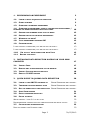
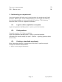
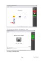
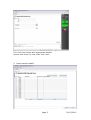
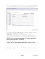
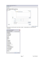
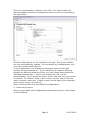
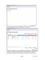
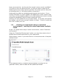
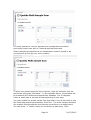
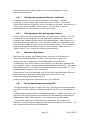
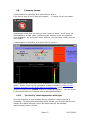
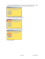
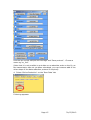
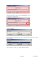
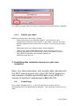
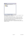
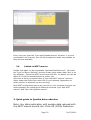
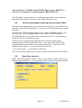
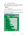
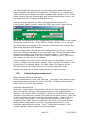
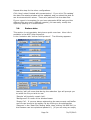
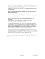
Quokka user manual
This guide is not intended to replace your local contact, but to
jog your memory if you are operating independently. Anything
strange, call your local contact…
Numbers for Quokka instrument scientists:
Elliot Gilbert, office – 9470, mobile – 04 09 03 43 05
Katy Wood, office – 7100, mobile – 04 17 47 35 37
Chris Garvey, office – 9328, mobile – 04 09 22 58 81
An image of the quokka detector is visible from outside ansto at the
following webpage:
http://www.nbi.ansto.gov.au/quokka/
Reactor status and cold source temperature visible at (do not leave this
webpage open for long periods of time):
http://prism.nbi.ansto.gov.au/reactor/ReactorInfo.swf
Other useful numbers:
Emergencies – SOSS: 888
SOSS (not emergency, working alone form etc…): 3434
Health Physics: 9779
IT helpdesk: 9200
Feedback on the manual: [email protected]
Page 1
30/07/2012
1.
PERFORMING AN EXPERIMENT
3
1.1.
LOGIN TO DATA ACQUISITION COMPUTER
3
1.2.
START GUMTREE
3
1.3.
STARTING A STANDARD EXPERIMENT
3
1.4.
STARTING AN EXPERIMENT USING A CONTROLLED ENVIRONMENT /
RUNNING THE SAME EXPERIMENT MULTIPLE TIMES
10
1.5.
SAVING RUN NUMBERS TABLE FOR LOG BOOK.
12
1.6.
SAVING REPORT FILE DURING EXPERIMENT.
12
1.7.
WHERE IS THE DATA?
12
1.8.
IS MY EXPERIMENT RUNNING OK?
12
1.9.
COMMON ISSUES
13
I HAVE STARTED A WORKFLOW, BUT WOULD LIKE TO STOP IT.
13
I HAVE STARTED A WORKFLOW, BUT WOULD LIKE TO PAUSE IT.
13
1.10.
‘ON THE FLY’ DATA INSPECTION WITH IGOR
13
1.11.
BEFORE YOU LEAVE
17
2. INSTALLING DATA REDUCTION MACROS ON YOUR OWN
COMPUTER
17
2.1.
INSTALL IGOR
17
2.2.
REMOVE ANY OLDER VERSIONS OF THE MACROS.
18
2.3.
INSTALL QUOKKA SPECIFIC MACROS
18
2.4.
SWITCH TO NIST MACROS
20
3.
QUICK GUIDE TO QUOKKA DATA REDUCTION
20
3.1.
LOGIN TO THE ANSTO NETWORK PC
ERROR! BOOKMARK NOT DEFINED.
3.2.
TRANSFER DATA AND REPORT FILES
ERROR! BOOKMARK NOT DEFINED.
3.3.
GET THE SENSITIVITY AND MASK FILES ERROR! BOOKMARK NOT DEFINED.
3.4.
OPEN IGOR MACROS
21
3.5.
SELECT WORKING DIRECTORY
22
3.6.
PATCH THE DATA
22
WRITE CORRECT λ AND ∆λ/λ TO ALL FILES
22
DETERMINE BEAM CENTRES FOR EACH CONFIGURATION AND WRITE TO FILE
23
3.7.
23
CALCULATING TRANSMISSIONS.
READ THE REPORT FILE & CREATE TABLE
Page 2
23
30/07/2012
CALCULATE TRANSMISSIONS
23
3.8.
24
REDUCE DATA
1. Performing an experiment
Your local contact will train you in how to enter the enclosure and load
samples. Before you do this independently you must sign the training
form to acknowledge you have received the training. The following
describes how to run the acquisition software.
1.1.
Login to data acquisition computer
Login and password will be given to you by your local contact
1.2.
Start gumtree
Currently version 1.5.7, link on desktop
Login and password will be given to you by your local contact
(Normally this would already be open. Caution – opening gumtree takes
some time).
1.3.
Starting a standard experiment
Below describes starting an experiment with the 20 position sample
changer at ambient temperature.
1. Select ‘multi-sample workflow’:
Page 3
30/07/2012
The following then appears (may take some time).
Click begin to start workflow.
Page 4
30/07/2012
Fill in first four boxes with appropriate details.
Ignore next three for now, then click ‘next’.
2. Insert sample details
Page 5
30/07/2012
The ‘drive to load position’ button allows you to move the sample changer
in the enclosure to a position where you can easily load your samples.
Once in this position insert your sample blocks into the changer.
Tick the boxes corresponding to where you have put samples, and enter
sample name, thickness and description.
In the ‘type’ pull down menu you can select either ‘SAMPLE’,
‘EMPTY_BEAM’. It’s best to treat your empty cell measurement as a
‘SAMPLE’. Making sure you have made the right selection simplifies data
processing.
Positions 19 and 20 on the sample changer are generally left with the
empty cell and empty beam, respectively.
‘Export CSV’ allows you to save a file with all sample names, thickness
etc.. in the different positions. This can then be re-loaded at a later stage
if you will be using similar sample names with the ‘Load CSV’ button.
The ‘Clear All’ and ‘Fill from Sample 1’ buttons are self-explanatory…
3. Select configurations
Clicking the ‘next’ button brings up the following screen, where you can
select your configurations:
Page 6
30/07/2012
Clicking the small green plus sign under ‘Configurations’ brings up the
following:
Page 7
30/07/2012
Click on a configuration to select it, then ‘OK’. Your local contact will
discuss suitable instrument configurations with you prior to commencing
the experiment.
Several configurations can be selected in this way. Red cross to delete
any you have added by mistake. Do not modify any configurations, only
your local contact should do this.
In the ‘transmission’ and ‘scattering’ boxes you enter the time the
samples will be measured for. (If you would like to measure different
samples for different amounts of time, you can change these values for
individual samples later – only for the ‘scattering’ runs, not the
transmissions). If you chose the ‘timer’ mode, enter the time you choose
in seconds. In ‘Counter’ mode, it will count to monitor and you should
enter a monitor count rate. A table is given on the right of the computer
with monitor counts, seconds etc…
Enter counting times in all the different configurations.
4. Select environment
Once you are happy with configurations and counting times, ‘next’ brings
up the following:
Page 8
30/07/2012
‘Normal’ environment is left selected if running with the 20 position
sample changer at ambient temperatures. Select ‘next’.
A table now appears with your samples and configurations. (Scroll across
to see all). If you do not with to measure all samples at all configurations,
you can uncheck the appropriate boxes. If you wish to do absolute
normalisation, always leave a transmission measurement of the empty
Page 9
30/07/2012
beam as we use this. At this point the ‘preset’ column can be modified if
you wish to count for different times. You do not need to measure the
scattering from the empty camera (position 20) unless you are using this
as a background (i.e. not using cuvette, solvent etc.).
Underneath the table an estimated experimental time is given. If you
change individual run times ‘Update’ will update this. If the runtime looks
very long, you’ve probably made an error and selected to count to monitor
counts but accidentally left the option selected as ‘time’.
Clicking ‘run’ then starts the run you have setup. If you have not opened
the shutter, you will see a prompt ‘shutter not open’. Check it’s open and
then ‘OK’ to start your run!
1.4.
Starting an experiment using a controlled
environment / running the same experiment multiple
times
As per 1.3 except that at step 4 ‘select environment’, select ‘Controlled
environment’.
Using the “Controlled Environment” option, you may then select a list of
sample environment controllers for your experiment.
Select dummy_motor if you would like to run the same series of samples
multiple times.
In the example above, 3 steps will be generated on clicking on the
‘generate’ button, and the table will be updated as follows:
Page 10
30/07/2012
It is then possible to run the samples and configurations selected
previously three times with a 2 second wait between each.
Select /sample/tc1/setpoint to use temperature control (needs to be
correctly set up first by your local contact).
To enter the preset values for the controller, type the numbers into the
text boxes and press “Generate”. In the example above, the samples will
be measured at 5 different temperatures, between 1 to 10 degrees.
Insert a small wait in seconds at the beginning of each step.
You may modify the preset values from the table if you do not wish to use
the fixed step presets generated by GumTree. The multi sample workflow
can support multiple sample environment controllers in an experiment.
You can press “+” button under the controller to add more. Each
Page 11
30/07/2012
additional controller simply adds a one more nested loop to your
experiment sequence.
1.5.
Saving run numbers table for log book.
As data is saved the run numbers appear in the table. It’s then
particularly useful to save this table with ‘export table’. This button
exports the table as a jpeg file, which can then be printed. Note that you
only export what is visible on the screen. (If you wish to save all
configurations you will have to scroll to the right).
1.6.
Saving report file during experiment.
At the end of a multi sample workflow, a ‘report’ file is created. This file
contains all the associations for the different configurations (which run
numbers are scattering files, which are transmissions, empty beam etc…),
and simplifies data reduction. If you’d like to treat your data before the
end, you can create a report file by hitting ‘Result Export’. If you want to
stop a multi-sample workflow early for some reason, make sure you
‘Result Export’ first, as this is not done automatically.
1.7.
Where is the data?
Data files are written and updated every minute in the directory in
/experiments/quokka/data/current. This directory is read only.
Report files are in /experiments/quokka/data/current/reports
A read/write copy of the data is also copied to the directory named after
the proposal number: /experiments/quokka/data/proposal/xxx. This data
can be patched etc… and used to do data reduction (see section 3). It is
updated approximately every 4 minutes.
At the end of the cycle the read only copy of the data and report files will
be moved into a directory named after the cycle number, eg.
/experiments/quokka/data/cycle/030
Links to these directories can be found on the desktop.
1.8.
Is my experiment running OK?
- As the workflow moves through your run, messages will be displayed at
the bottom in the ‘console’ indicating progress. Any errors will appear in
red.
- Approximate counts/rates on ‘standard’ samples. A table is given in the
log book with approximate count rates for some standard configurations
measured on H2O, D2O samples. You should have similar values.
- Instrument dashboard: The dashboard displays a 2D image of the
detector, most instrument settings and parameters such as L1 and L2. Do
not modify anything from this dashboard.
Page 12
30/07/2012
1.9.
Common issues
I have started a workflow, but would like to stop it.
Click on the any of the ‘Interrupt buttons’. A report file will be saved.
Multisample work flow will then go into ‘cleanup mode’, ie will drive the
attenuation to a high value, protecting the detector from any possible
over-exposure. By using the ‘back’ buttons, you can then modify the run
and restart.
I have started a workflow, but would like to pause it.
The workflow can be paused if the acquisition is running in the monitor
mode. Firstly, open up the histogram memory website on http://das1quokka.nbi.ansto.gov.au:8080/admin/viewdata.egi, (book-marked in
firefox) and press the yellow button to pause the system. You can press
on the same button to resume from a paused acquisition.
1.10.
‘On the fly’ data inspection with Igor
It is now possible to look at data during collection, before the file is
complete. Following the procedure below allows you to open the file and
inspect the radial average, which will automatically be updated
approximately every minute.
Page 13
30/07/2012
1. Open “Igor with Quokka macros”, and in the macros menu select ‘Load
Quokka Sans Reduction Macros’. Following yellow panel appears.
2. Click on ‘Pick Path’ and navigate to
/experiments/quokka/data/proposal/xxx
3. In the ‘Reduction’ tab ‘Build protocol’.
Following appears:
Page 14
30/07/2012
Uncheck all except Sample and Average and ‘Save protocol’. Choose a
name eg ‘on_line’.
(Note that it is not possible to put data on an absolute scale on the fly, as
the transmission has not yet been calculated, you can however add in the
other steps of the data reduction protocol if required).
4. Select ‘Online Reduction’ on the ‘Raw Data’ tab
Following appears:
Page 15
30/07/2012
Select the file file you would like in top drop down menu.
In the second window click ‘…’,
following appears:
Select the protocol you have just built in the drop down menu, eg ‘on_line’
and ‘continue’.
Then click ‘start’ on the pink ‘Online Reduction panel’.
Page 16
30/07/2012
The radial average data will then be displayed and automatically updated.
1.11.
Before you leave
Before you leave the instrument, please:
-
Clean and return your sample holders. Instructions in the
‘instructions’ section of the manual in the cabin. We will not lend
sample holders to users who have a history of not returning them
clean.
-
Photocopy/scan the relevant pages of the logbook.
-
Take all raw and treated data either using a thumb drive, by
burning the data to a CD/DVD (ask your local contact nicely) or
using ANSTO sharefile (web-based system) at
sharefile.ansto.gov.au.
2. Installing data reduction macros on your own
computer
Note: Any data publication with quokka data reduced with
the NIST macros should cite: Kline SR (2006) Reduction
and analysis of SANS and USANS data using IGOR Pro.
Journal of Applied Crystallography 39: 895-900
2.1.
Install Igor
If you don’t already have it… A free 30 day demo version can be
downloaded from the wavemetrics website. You need Igor version 6.2 or
later.
Page 17
30/07/2012
2.2.
Remove any older versions of the macros.
Skip this step if you’ve never had any of the NIST or Quokka macros
installed. If you’ve had any older versions of the NIST or Quokka analysis
macros installed, it’s important to remove completely/rename folder so
there will be no conflicts. You will only have to do this once, as the future
updates will be done automatically as long as you are connected to the
internet.
! Caution – once you have installed the newer versions of the macros,
you will not be able to load any Igor project files made with the older
ones. This means you should save all the treated asquii files you are
likely to need before installing a newer version of the software.
1) Delete any old NIST and Quokka macros from the following directories
(or move all macros elsewhere if you’d like to keep older versions of the
macros):
•
C:\Program Files\WaveMetrics\Igor Pro Folder\User Procedures
•
C:\Documents and Settings\user_name\My
Documents\WaveMetrics\Igor Pro 6 User Files\User Procedures
•
C:\Documents and Settings\user_name\My
Documents\WaveMetrics\Igor Pro 6 User Files\Igor Procedures
2) Delete the two shortcuts to HDF5.xop and HDF5 Browser.ipf in:
C:\Program Files\WaveMetrics\Igor Pro Folder\Igor Extensions
2.3.
Install Quokka specific macros
Navigate to:
http://www.nbi.ansto.gov.au/quokka/macros/IgorUserFilesSwitch.exe
and download the executable ‘IgorUserFilesSwitch.exe’. Double click on
the executable.
Page 18
30/07/2012
Select Quokka macros to install and click OK. You will be asked if it is OK
to download the macros, select yes.
After installation ‘continue’ will launch Igor. Ticking the ‘continue when
done box’ will automatically start Igor after you have used the switch.
Once this is done you should have a “Igor with Quokka macros” shortcut
either under the Start>Igor menu OR on your desktop (depending on
which version of windows you are running).
Once Igor Pro is open, the Macros menu should now contain ‘Load
QUOKKA SANS Reduction Macros’. Selecting this brings up yellow ‘SANS
Reduction Controls’.
Page 19
30/07/2012
Every time you open the “Igor with Quokka macros” shortcut, if you are
connected to the internet, you will be prompted to install any updates as
they become available.
2.4.
Switch to NIST macros
Double click again on the executable ‘IgorUserFilesSwitch.exe’. (Or select
the “Igor Pro Macro Settings” shortcut under either under start>Igor or on
the desktop). Select the NIST macros and click OK. As above, you will be
asked if it is OK to download macros, select yes.
Once this is done you should have a “Igor with NIST macros” shortcut
either under the Start>Igor menu OR on your desktop (depending on
which version of windows you are running).
Both NIST and Quokka macros will now be on your computer and you can
switch between by selecting the different shortcuts “Igor with NIST
macros” and “Igor with Quokka macros”.
3. Quick guide to Quokka data reduction
Note: Any data publication with quokka data reduced with
the NIST macros should cite: Kline SR (2006) Reduction
Page 20
30/07/2012
and analysis of SANS and USANS data using IGOR Pro.
Journal of Applied Crystallography 39: 895-900
The following is a ‘quick guide’ to treating quokka data. More detailled
help about the macros is found in the ‘help’ buttons in Igor.
3.1.
Chose a workspace and copy across report files
Data can be treated either on the instrument control PC, or the NBI PC on
the left in cabin (DAV2-Quokka), or your own PC with Quokka Igor macros
installed.
If working on DAV2-Quokka, please work under D:\Quokka Users. Any
old (pre- April 2012) reduced data is now under D:\NSVIS.backup.
On DAV2-Quokka, your data can be copied across from J:\proposal\xxx
where xxx is your proposal number.
Report files are saved which associates the relevant transmission
measurements with the scattering files – copy across the report files
associated with your data to your working directory. These are under
/data/current/reports
J:\current\reports
on the Instrument control PC.
on the DAV2-quokka PC.
Your local contact should give you the relevant sensitivity and mask files.
3.2.
Open Igor macros
Open “Igor with Quokka macros”, then in the ‘Macros’ menu select ‘Load
Quokka data reduction’. You should be able to see the following window:
Page 21
30/07/2012
3.3.
Select working directory
On the SANS Reduction controls, ‘Pick path’ (select path where all your
data is), then ‘file catalogue’. A table with all data files + characteristics
appears, this table takes some time to appear the first time, the small
sign on the bottom left of Igor tells you it’s working....
3.4.
Patch the data
This step is only necessary on data taken prior to April 2011, later data
does not need to be patched, unless advised by your local contact.
Write correct λ and ∆λ/λ to all files
Select ‘patch’ on the ‘raw data’ tab. With a * in the ‘match string’ box, hit
enter. The ‘files to patch’ drop down menu should then be populated with
all the files in your working directory.
Page 22
30/07/2012
The wavelength and wavelength spread values have been measured
experimentally and should be changed to 5.078 and 0.14, respectively.
These values are for data collected on Quokka after October 2010. Enter
these number into the ‘Wavelength’ and ‘Wavelength spread’ boxes, tick
the boxes and click ‘Change All Headers in List’.
Determine beam centres for each configuration and write to file
In the green ‘patch’ window, select the ‘SDD’ box under ‘Match String’.
Enter the SDD distance of the configuration you wish to treat in the ‘Match
String’ box and hit enter. If the SDD=1.31531, writing 1.3* is enough.
The drop down menu under ‘Files to patch’ should now only contain the
files at the specified SDD distance.
Select a transmission file for the first configuration you wish to treat by
usinig the ‘Display raw data’ in the ‘raw data’ tab. Select the direct beam
using the marquee, right click and ‘find beam centre’. The X and Ycenters will be displayed in the Igor ‘history’ window (cntrl +J will bring
this window to the front if it is hidden).
Copy and paste the beam centre values which are displayed in the Igor
‘history’ window into the ‘patch’ window. Then ‘change all headers in List’.
By selecting ‘File catalog’ again, the table ‘Data File Catalog’ will be
refreshed and the columns Xcenter and Ycenter should be filled.
Repeat this step for the other configurations you wish to treat.
3.5.
Calculating transmissions.
Read the report file & create table
Select ‘transmission’ in the ‘raw data’ tab. ‘pick path’ then select the xml
report generated by gumtree, then ‘List Files’. A table is then created
with all the correct file associations.
Calculate transmissions
Select the ‘empty beam’ transmission file for the first configuration you
want to treat by clicking on the appropriate box in the table (should
appear in the column ‘EMP_Filenames’), and click ‘set BCENT file’ on the
‘calculate transmissions’ window (this sets this to beam centre). Click ‘Set
XY Box’ and use the square to select the beam centre. Right click and
select ‘SetXY box coords’. Then highlight the scattering files in the
‘scattering files table’ at the configuration for which you’ve just set the
empty beam transmission, and click ‘calculate selected files’ in the
Calculate transmissions window. The S_Transmission column in the
‘ScatteringFiles’ window should now be populated.
Page 23
30/07/2012
Repeat this step for the other configuations.
Click ‘done’ when finished with transmissions’. If you click ‘File catalog’
the data File catalog window will be updated, and you should be able to
see the transmission values. These are ‘patched’ into the data files.
If your report is incomplete (ie you have stopped a MSW early and the
different files are now in different reports) you can easily modify the
report by opening it in a text editor.
3.6.
Reduce data
This section is not complete, but gives a quick overview. More info is
available in the NIST help document.
In the ‘reduction tab’ choose ‘build protocol’. The following appears:
Leaving ‘ask’ will mean that during the reduction Igor will prompt you
to select the file you wish to use:
‘Sample’ will typically remain ‘ask’.
‘Background’ is a scan of the blocked beam.
‘Empty Cell’. If you are always subtracting the same empty cell/buffer
run this can be set to the empty file by clicking on the appropriate
‘filename’ in the ‘Data File Catalog’ table, then clicking ‘set EMP file’ (or
the filename can be copied and pasted in). (If you are using an empty
Page 24
30/07/2012
cell from a previous run, you need to copy the file to the current
directory – these will have different beam centres, unless obviously far
off warnings about this can be ignored).
‘Sensitivity’. Take the sensitivity file in S:\Bragg\Quokka\Sensitivity
and standards\
or one given by your local contact. Copy and paste the sensitivity file
name or select it in the ‘data file catalog’, then ‘set DIV file’ on the
data reduction window.
‘Absolute’ – for absolute scaling. Click ‘set ABS params’, then select
method of absolute calibration ‘Empty Beam Flux’. Select the empty
beam transmission file, and draw a box around the beam with the
cursor, then click ‘continue’.
‘Mask’. Take the mask file in S:\Bragg\Quokka\Sensitivity and
standards\
or one given by your local contact, or make up your own!
‘Average’ can be left as is for isotropic data.
The data reduction protocol that you’ve now created can be saved
‘Save Protocol’. You can now reduce a file by selecting ‘Reduce a file’
directly in the blue ‘Data Reduction Protocol’ panel, or if you have
saved the protocol, directly on the yellow ‘SANS Reduction Control’
panel. Via the ‘SANS Reduction Control’ panel you can then select the
protocol (useful if you want to make multiple protocols).
During the reduction, you’ll be prompted to select files to use. Each
time Igor asks ‘Do you want to add another xxx file’? This is for if you
wish to add multiple runs together, if you only have one run, select no.
Reduced data are then saved in the file: QKK00xxx.ABS
To merge several configurations configurations together: 1D Ops, ‘sort’
button
Page 25
30/07/2012