1
NIST Special Publication 1018-5
Fire Dynamics Simulator (Version 5)
Technical Reference Guide
Volume 2: Verification
Randall McDermott
Kevin McGrattan
Simo Hostikka
Jason Floyd
NIST Special Publication 1018-5
Fire Dynamics Simulator (Version 5)
Technical Reference Guide
Volume 2: Verification
Randall McDermott
Kevin McGrattan
Fire Research Division
Building and Fire Research Laboratory
Simo Hostikka
VTT Technical Research Centre of Finland
Espoo, Finland
Jason Floyd
Hughes Associates, Inc.
Baltimore, Maryland
N T OF C O M
M
IT
E
D
ER
UN
ICA
E
D EP
E
TM
C
ER
AR
October 29, 2010
FDS Version 5.5
SV NRepository Revision : 6843
ST
ATES OF
AM
U.S. Department of Commerce
Gary Locke, Secretary
National Institute of Standards and Technology
Patrick Gallagher, Director
Preface
This is Volume 2 of the FDS Technical Reference Guide. Volume 1 describes the mathematical model and
numerical method. Volume 3 documents past and present experimental validation work. Instructions for
using FDS are contained in a separate User’s Guide [1].
The three volumes of the FDS Technical Reference Guide are based in part on the “Standard Guide
for Evaluating the Predictive Capability of Deterministic Fire Models,” ASTM E 1355 [2]. ASTM E 1355
defines model evaluation as “the process of quantifying the accuracy of chosen results from a model when
applied for a specific use.” The model evaluation process consists of two main components: verification
and validation. Verification is a process to check the correctness of the solution of the governing equations.
Verification does not imply that the governing equations are appropriate; only that the equations are being
solved correctly. Validation is a process to determine the appropriateness of the governing equations as a
mathematical model of the physical phenomena of interest. Typically, validation involves comparing model
results with experimental measurement. Differences that cannot be explained in terms of numerical errors
in the model or uncertainty in the measurements are attributed to the assumptions and simplifications of the
physical model.
Evaluation is critical to establishing both the acceptable uses and limitations of a model. Throughout
its development, FDS has undergone various forms of evaluation, both at NIST and beyond. This volume
provides a survey of verification work conducted to date to evaluate FDS.
i
ii
About the Authors
Randall McDermott joined the research staff of the Building and Fire Research Lab in 2008. He received
a B.S. degree from the University of Tulsa in Chemical Engineering in 1994 and a doctorate at the
University of Utah in 2005. His research interests include subgrid-scale models and numerical methods for large-eddy simulation, adaptive mesh refinement, Lagrangian particle methods, and immersed
boundary methods.
Kevin McGrattan is a mathematician in the Building and Fire Research Laboratory (BFRL) of NIST.
He received a bachelors of science degree from the School of Engineering and Applied Science of
Columbia University in 1987 and a doctorate at the Courant Institute of New York University in 1991.
He joined the NIST staff in 1992 and has since worked on the development of fire models, most
notably the Fire Dynamics Simulator.
Simo Hostikka is a Senior Research Scientist at VTT Technical Research Centre of Finland. He received
a master of science (technology) degree in 1997 and a doctorate in 2008 from the Department of
Engineering Physics and Mathematics of the Helsinki University of Technology. He is the principal
developer of the radiation and solid phase sub-models within FDS.
Jason Floyd is a Senior Engineer at Hughes Associates, Inc., in Baltimore, Maryland. He received a bachelors of science and Ph.D. in the Nuclear Engineering Program of the University of Maryland. After
graduating, he won a National Research Council Post-Doctoral Fellowship at the Building and Fire
Research Laboratory of NIST, where he developed the combustion algorithm within FDS. He is currently funded by NIST under grant 70NANB8H8161 from the Fire Research Grants Program (15 USC
278f). He is the principal developer of the multi-parameter mixture fraction combustion model and
control logic within FDS.
iii
iv
Acknowledgments
FDS is supported financially via internal funding at both NIST and VTT, Finland. In addition, support is
provided by other agencies of the US Federal Government:
• The US Nuclear Regulatory Commission Office of Research has funded key validation experiments,
the preparation of the FDS manuals, and the development of various sub-models that are of importance
in the area of nuclear power plant safety. Special thanks to Mark Salley and Jason Dreisbach for their
efforts and support. The Office of Nuclear Material Safety and Safeguards, another branch of the US
NRC, has supported modeling studies of tunnel fires under the direction of Chris Bajwa and Allen
Hansen.
• The Micro-Gravity Combustion Program of the National Aeronautics and Space Administration (NASA)
has supported several projects that directly or indirectly benefited FDS development.
• The US Forest Service has supported the development of sub-models in FDS designed to simulate the
spread of fire in the Wildland Urban Interface (WUI). Special thanks to Mark Finney and Tony Bova
for their support.
• The Minerals Management Service of the US Department of the Interior funded research at NIST
aimed at characterizing the burning behavior of oil spilled on the open sea or ice. Part of this research
led to the development of the ALOFT (A Large Outdoor Fire plume Trajectory) model, a forerunner
of FDS. Special thanks to Joe Mullin for his encouragement of the modeling efforts.
The following individuals and organizations played a role in the verification process of FDS.
• Thanks to Chris Lautenburger and Carlos Fernandez-Pello for their assistance with the “two-reaction”
test case.
• Matthias Münch of the Freie Universität Berlin provided useful test cases for the basic flow solver.
• Susanne Kilian of hhpberlin (Germany) helped to debug the improved pressure solver.
• Clara Cruz, a student at the University of Puerto Rico and Summer Undergraduate Fellow at NIST,
helped developed useful Matlab scripts to automate the process of compiling this Guide.
• Bryan Klein of NIST developed the source code version control system that is an essential part of the
verification process.
• Anna Matala of VTT, Finland, designed the “surf mass” pyrolysis cases.
• Danielle Antonellis, a student at Worcester Polytechnic Institute and Summer Undergraduate Fellow
at NIST, added the pulsating scalar verification test case.
v
vi
Contents
Preface
i
About the Authors
iii
Acknowledgments
v
1
What is Verification?
1
2
Survey of Past Verification Work
2.1 Analytical Tests . . . . . . . . . . . . . . . . . . . . . . . . . .
2.2 Numerical Tests . . . . . . . . . . . . . . . . . . . . . . . . . .
2.3 Sensitivity Analysis . . . . . . . . . . . . . . . . . . . . . . . .
2.3.1 Grid Sensitivity . . . . . . . . . . . . . . . . . . . . . .
2.3.2 Sensitivity of Large Eddy Simulation Parameters . . . .
2.3.3 Sensitivity of Radiation Parameters . . . . . . . . . . .
2.3.4 Sensitivity of Thermophysical Properties of Solid Fuels .
2.4 Code Checking . . . . . . . . . . . . . . . . . . . . . . . . . .
3
The Basic Flow Solver
3.1 2D Analytical Solution to Navier-Stokes . . . . . . . . . . . . .
3.2 Decaying Isotropic Turbulence . . . . . . . . . . . . . . . . . .
3.3 The Dynamic Smagorinsky Model . . . . . . . . . . . . . . . .
3.4 FDS Wall Flows Part I: Straight Channels . . . . . . . . . . . .
3.4.1 Formulation . . . . . . . . . . . . . . . . . . . . . . . .
3.4.2 Results . . . . . . . . . . . . . . . . . . . . . . . . . .
3.4.3 Conclusions . . . . . . . . . . . . . . . . . . . . . . . .
3.5 Analytical Solutions to the Continuity Equation . . . . . . . . .
3.5.1 Pulsating 1D solution . . . . . . . . . . . . . . . . . . .
3.5.2 Pulsating 2D solution . . . . . . . . . . . . . . . . . . .
3.5.3 Stationary compression wave in 1D . . . . . . . . . . .
3.5.4 Stationary compression wave in 2D . . . . . . . . . . .
3.6 Scalar Transport (move_slug) . . . . . . . . . . . . . . . . . . .
3.7 Energy Conservation (energy_budget) . . . . . . . . . . . . . .
3.7.1 The Heat from a Fire (energy_budget) . . . . . . . . .
3.7.2 Gas Injection via an Isentropic Process (isentropic) . . .
3.7.3 Gas Injection via a Non-Isentropic Process (isentropic2)
3.8 Checking for Coding Errors (symmetry_test) . . . . . . . . . .
vii
.
.
.
.
.
.
.
.
.
.
.
.
.
.
.
.
.
.
.
.
.
.
.
.
.
.
.
.
.
.
.
.
.
.
.
.
.
.
.
.
.
.
.
.
.
.
.
.
.
.
.
.
.
.
.
.
.
.
.
.
.
.
.
.
.
.
.
.
.
.
.
.
.
.
.
.
.
.
.
.
.
.
.
.
.
.
.
.
.
.
.
.
.
.
.
.
.
.
.
.
.
.
.
.
.
.
.
.
.
.
.
.
.
.
.
.
.
.
.
.
.
.
.
.
.
.
.
.
.
.
.
.
.
.
.
.
.
.
.
.
.
.
.
.
.
.
.
.
.
.
.
.
.
.
.
.
.
.
.
.
.
.
.
.
.
.
.
.
.
.
.
.
.
.
.
.
.
.
.
.
.
.
.
.
.
.
.
.
.
.
.
.
.
.
.
.
.
.
.
.
.
.
.
.
.
.
.
.
.
.
.
.
.
.
.
.
.
.
.
.
.
.
.
.
.
.
.
.
.
.
.
.
.
.
.
.
.
.
.
.
.
.
.
.
.
.
.
.
.
.
.
.
.
.
.
.
.
.
.
.
.
.
.
.
.
.
.
.
.
.
.
.
.
.
.
.
.
.
.
.
.
.
.
.
.
.
.
.
.
.
.
.
.
.
.
.
.
.
.
.
.
.
.
.
.
.
.
.
.
.
.
.
.
.
.
.
.
.
.
.
.
.
.
.
.
.
.
.
.
.
.
.
.
.
.
.
.
.
.
.
.
.
.
.
.
.
.
.
.
.
.
.
.
.
.
.
.
.
.
.
.
.
.
.
.
.
.
.
.
.
.
.
3
3
4
5
5
7
7
8
9
.
.
.
.
.
.
.
.
.
.
.
.
.
.
.
.
.
.
11
11
15
18
20
20
21
22
25
25
26
27
27
30
32
32
32
33
36
4
Thermal Radiation
4.1 Radiation from parallel plate in different co-ordinate systems
(plate_view_factor) . . . . . . . . . . . . . . . . . . . . . .
4.2 Radiation inside a box (radiation_in_a_box) . . . . . . . . .
4.3 Radiation from a plane layer (radiation_plane_layer) . . . .
4.4 Wall Internal Radiation (wall_internal_radiation) . . . . . .
4.5 Radiation Emitted by Hot Spheres (hot_spheres) . . . . . . .
4.6 Radiation Absorbed by Liquid Droplets (droplet_absorption)
37
.
.
.
.
.
.
.
.
.
.
.
.
.
.
.
.
.
.
.
.
.
.
.
.
.
.
.
.
.
.
.
.
.
.
.
.
.
.
.
.
.
.
.
.
.
.
.
.
.
.
.
.
.
.
.
.
.
.
.
.
.
.
.
.
.
.
.
.
.
.
.
.
.
.
.
.
.
.
.
.
.
.
.
.
.
.
.
.
.
.
.
.
.
.
.
.
38
39
40
41
42
43
5
Species and Combustion
45
5.1 Boundary Conditions . . . . . . . . . . . . . . . . . . . . . . . . . . . . . . . . . . . . . . 45
5.1.1 Specified Mass Flux (low_flux_hot_gas_filling) . . . . . . . . . . . . . . . . . . . . 45
5.2 Fractional Effective Dose (FED_Device) . . . . . . . . . . . . . . . . . . . . . . . . . . . 46
6
Heat Conduction
49
6.1 Simple Heat Conduction Through a Solid Slab (heat_conduction) . . . . . . . . . . . . . . 50
6.2 Temperature-Dependent Thermal Properties (heat_conduction_kc) . . . . . . . . . . . . . 51
6.3 Simple Thermocouple Model (thermocouples) . . . . . . . . . . . . . . . . . . . . . . . . 52
7
Pyrolysis
7.1 Mass conservation of pyrolyzed mass (surf_mass_conservation) .
7.1.1 Pyrolysis at a Solid Surface . . . . . . . . . . . . . . . .
7.1.2 Pyrolysis of Discrete Particles . . . . . . . . . . . . . . .
7.2 Development of surface emissivity (emissivity) . . . . . . . . . .
7.3 Enthalpy of solid materials (enthalpy) . . . . . . . . . . . . . . .
7.4 A Simple Two-Step Pyrolysis Example (two_step_solid_reaction)
7.5 Interpreting Bench-Scale Measurements . . . . . . . . . . . . . .
7.5.1 General Theory . . . . . . . . . . . . . . . . . . . . . . .
7.5.2 Using Micro-Calorimetry Data (cable_11_mcc) . . . . . .
7.5.3 Using TGA Data (birch_tga) . . . . . . . . . . . . . . .
8
.
.
.
.
.
.
.
.
.
.
.
.
.
.
.
.
.
.
.
.
.
.
.
.
.
.
.
.
.
.
.
.
.
.
.
.
.
.
.
.
.
.
.
.
.
.
.
.
.
.
.
.
.
.
.
.
.
.
.
.
.
.
.
.
.
.
.
.
.
.
.
.
.
.
.
.
.
.
.
.
.
.
.
.
.
.
.
.
.
.
.
.
.
.
.
.
.
.
.
.
.
.
.
.
.
.
.
.
.
.
.
.
.
.
.
.
.
.
.
.
.
.
.
.
.
.
.
.
.
.
.
.
.
.
.
.
.
.
.
.
53
53
54
57
60
61
62
63
63
64
66
Lagrangian Particles
67
8.1 Momentum Transfer (particle_drag) . . . . . . . . . . . . . . . . . . . . . . . . . . . . . 67
8.2 Water Droplet Evaporation (water_evaporation) . . . . . . . . . . . . . . . . . . . . . . . 69
Bibliography
71
viii
Chapter 1
What is Verification?
The terms verification and validation are often used interchangeably to mean the process of checking the
accuracy of a numerical model. For many, this entails comparing model predictions with experimental
measurements. However, there is now a fairly broad-based consensus that comparing model and experiment
is largely what is considered validation. So what is verification? ASTM E 1355 [2], “Standard Guide for
Evaluating the Predictive Capability of Deterministic Fire Models,” defines verification as
The process of determining that the implementation of a calculation method accurately represents the developer’s conceptual description of the calculation method and the solution to the
calculation method.
and it defines validation as
The process of determining the degree to which a calculation method is an accurate representation of the real world from the perspective of the intended uses of the calculation method.
Simply put, verification is a check of the math; validation is a check of the physics. If the model predictions
closely match the results of experiments, using whatever metric is appropriate, it is assumed by most that
the model suitably describes, via its mathematical equations, what is happening. It is also assumed that the
solution of these equations must be correct. So why do we need to perform model verification? Why not
just skip to validation and be done with it? The reason is that rarely do model and measurement agree so
well in all applications that anyone would just accept its results unquestionably. Because there is inevitably
differences between model and experiment, we need to know if these differences are due to limitations or
errors in the numerical solution, or the physical sub-models, or both.
Whereas model validation consists mainly of comparing predictions with measurements, as documented
for FDS in Volume 3 of the Technical Reference Guide, model verification consists of a much broader range
of activities, from checking the computer program itself to comparing calculations to analytical (exact)
solutions to considering the sensitivity of the dozens of numerical parameters. The next chapter discusses
these various activities, and the rest of the Guide is devoted mainly to comparisons of various sub-model
calculations with analytical solutions.
1
2
Chapter 2
Survey of Past Verification Work
This chapter documents work of the past few decades at NIST, VTT and elsewhere to verify the algorithms
within FDS.
2.1
Analytical Tests
Most complex combustion processes, including fire, are turbulent and time-dependent. There are no closedform mathematical solutions for the fully-turbulent, time-dependent Navier-Stokes equations. CFD provides
an approximate solution for the non-linear partial differential equations by replacing them with discretized
algebraic equations that can be solved using a powerful computer. While there is no general analytical
solution for fully-turbulent flows, certain sub-models address phenomenon that do have analytical solutions,
for example, one-dimensional heat conduction through a solid. These analytical solutions can be used to
test sub-models within a complex code such as FDS. The developers of FDS routinely use such practices to
verify the correctness of the coding of the model [3, 4]. Such verification efforts are relatively simple and
routine and the results may not always be published nor included in the documentation. Examples of routine
analytical testing include:
• The radiation solver has been verified with scenarios where simple objects, like cubes or flat plates,
are positioned in simple, sealed compartments. All convective motion is turned off, the object is given
a fixed surface temperature and emissivity of one (making it a black body radiator). The heat flux
to the cold surrounding walls is recorded and compared to analytical solutions. These studies help
determine the appropriate number of solid angles to be set as the default.
• Solid objects are heated with a fixed heat flux, and the interior and surface temperatures as a function
of time are compared to analytical solutions of the one-dimensional heat transfer equation. These
studies help determine the number of nodes to use in the solid phase heat transfer model. Similar
studies are performed to check the pyrolysis models for thermoplastic and charring solids.
• Early in its development, the hydrodynamic solver that evolved to form the core of FDS was checked
against analytical solutions of simplified fluid flow phenomena. These studies were conducted at the
National Bureau of Standards (NBS)1 by Rehm, Baum and co-workers [5, 6, 7, 8]. The emphasis
of this early work was to test the stability and consistency of the basic hydrodynamic solver, especially the velocity-pressure coupling that is vitally important in low Mach number applications. Many
numerical algorithms developed up to that point in time were intended for use in high-speed flow
applications, like aerospace. Many of the techniques adopted by FDS were originally developed for
1 The
National Institute of Standards and Technology (NIST) was formerly known as the National Bureau of Standards.
3
meteorological models, and as such needed to be tested to assess whether they would be appropriate
to describe relatively low-speed flow within enclosures.
• A fundamental decision made by Rehm and Baum early in the FDS development was to use a direct
(rather than iterative) solver for the pressure. In the low Mach number formulation of the NavierStokes equations, an elliptic partial differential equation for the pressure emerges, often referred to as
the Poisson equation. Most CFD methods use iterative techniques to solve the governing conservation
equations to avoid the necessity of directly solving the Poisson equation. The reason for this is that
the equation is time-consuming to solve numerically on anything but a rectilinear grid. Because FDS
is designed specifically for rectilinear grids, it can exploit fast, direct solvers of the Poisson equation,
obtaining the pressure field with one pass through the solver to machine accuracy. FDS employs
double-precision (8 byte) arithmetic, meaning that the relative difference between the computed and
the exact solution of the discretized Poisson equation is on the order of 10−12 . The fidelity of the
numerical solution of the entire system of equations is tied to the pressure/velocity coupling because
often simulations can involve hundreds of thousands of time steps, with each time step consisting of
two solutions of the Poisson equation to preserve second-order accuracy. Without the use of the direct
Poisson solver, build-up of numerical error over the course of a simulation could produce spurious
results. Indeed, an attempt to use single-precision (4 byte) arithmetic to conserve machine memory
led to spurious results simply because the error per time step built up to an intolerable level.
2.2
Numerical Tests
Numerical techniques used to solve the governing equations within a model can be a source of error in
the predicted results. The hydrodynamic model within FDS is second-order accurate in space and time.
This means that the error terms associated with the approximation of the spatial partial derivatives by finite
differences is of the order of the square of the grid cell size, and likewise the error in the approximation of
the temporal derivatives is of the order of the square of the time step. As the numerical grid is refined, the
“discretization error” decreases, and a more faithful rendering of the flow field emerges. The issue of grid
sensitivity is extremely important to the proper use of the model and will be taken up in the next chapter.
A common technique of testing flow solvers is to systematically refine the numerical grid until the
computed solution does not change, at which point the calculation is referred to as a Direct Numerical
Solution (DNS) of the governing equations. For most practical fire scenarios, DNS is not possible on
conventional computers. However, FDS does have the option of running in DNS mode, where the NavierStokes equations are solved without the use of sub-grid scale turbulence models of any kind. Because
the basic numerical method is the same for LES and DNS, DNS calculations are a very effective way to
test the basic solver, especially in cases where the solution is steady-state. Throughout its development,
FDS has been used in DNS mode for special applications. For example, FDS (or its core algorithms)
have been used at a grid resolution of roughly 1 mm to look at flames spreading over paper in a microgravity
environment [9, 10, 11, 12, 13, 14], as well as "g-jitter" effects aboard spacecraft [15]. Simulations have been
compared to experiments performed aboard the US Space Shuttle. The flames are laminar and relatively
simple in structure, and the comparisons are a qualitative assessment of the model solution. Similar studies
have been performed comparing DNS simulations of a simple burner flame to laboratory experiments [16].
Another study compared FDS simulations of a counterflow diffusion flames to experimental measurements
and the results of a one-dimensional multi-step kinetics model [17].
Early work with the hydrodynamic solver compared two-dimensional simulations of gravity currents
with salt-water experiments [18]. In these tests, the numerical grid was systematically refined until almost
perfect agreement with experiment was obtained. Such convergence would not be possible if there were a
fundamental flaw in the hydrodynamic solver.
4
2.3
Sensitivity Analysis
A sensitivity analysis considers the extent to which uncertainty in model inputs influences model output.
Model parameters can be the physical properties of solids and gases, boundary conditions, initial conditions,
etc. The parameters can also be purely numerical, like the size of the numerical grid. FDS typically requires
the user to provide several dozen different types of input parameters that describe the geometry, materials,
combustion phenomena, etc. By design, the user is not expected to provide numerical parameters besides the
grid size, although the optional numerical parameters are described in both the Technical Reference Guide
and the User’s Guide.
FDS does not limit the range of most of the input parameters because applications often push beyond
the range for which the model has been validated. FDS is still used for research at NIST and elsewhere,
and the developers do not presume to know in all cases what the acceptable range of any parameter is. Plus,
FDS solves the fundamental conservation equations and is much less susceptible to errors resulting from
input parameters that stray beyond the limits of simpler empirical models. However, the user is warned that
he/she is responsible for the prescription of all parameters. The FDS manuals can only provide guidance.
The grid size is the most important numerical parameter in the model, as it dictates the spatial and temporal accuracy of the discretized partial differential equations. The heat release rate is the most important
physical parameter, as it is the source term in the energy equation. Property data, like the thermal conductivity, density, heat of vaporization, heat capacity, etc., ought to be assessed in terms of their influence on
the heat release rate. Validation studies have shown that FDS predicts well the transport of heat and smoke
when the HRR is prescribed. In such cases, minor changes in the properties of bounding surfaces do not
have a significant impact on the results. However, when the HRR is not prescribed, but rather predicted
by the model using the thermophysical properties of the fuels, the model output is sensitive to even minor
changes in these properties.
The sensitivity analyses described in this chapter are all performed in basically the same way. For a given
scenario, best estimates of all the relevant physical and numerical parameters are made, and a “baseline”
simulation is performed. Then, one by one, parameters are varied by a given percentage, and the changes
in predicted results are recorded. This is the simplest form of sensitivity analysis. More sophisticated
techniques that involve the simultaneous variation of several parameters are impractical with a CFD model
because the computation time is too long and the number of parameters too large to perform the necessary
number of calculations to generate decent statistics.
2.3.1
Grid Sensitivity
The most important decision made by a model user is the size of the numerical grid. In general, the finer the
numerical grid, the better the numerical solution of the equations. FDS is second-order accurate in space and
time, meaning that halving the grid cell size will decrease the discretization error in the governing equations
by a factor of 4. Because of the non-linearity of the equations, the decrease in discretization error does not
necessarily translate into a comparable decrease in the error of a given FDS output quantity. To find out
what effect a finer grid has on the solution, model users usually perform some form of grid sensitivity study
in which the numerical grid is systematically refined until the output quantities do not change appreciably
with each refinement. Of course, with each halving of the grid cell size, the time required for the simulation
increases by a factor of 24 = 16 (a factor of two for each spatial coordinate, plus time). In the end, a
compromise is struck between model accuracy and computer capacity.
Some grid sensitivity studies have been documented and published. Since FDS was first publicly released in 2000, significant changes in the combustion and radiation routines have been incorporated into the
model. However, the basic transport algorithm is the same, as is the critical importance of grid sensitivity. In
compiling sensitivity studies, only those that examined the sensitivity of routines no longer used have been
5
excluded.
As part of a project to evaluate the use of FDS version 1 for large scale mechanically ventilated enclosures, Friday [19] performed a sensitivity analysis to find the approximate calculation time based on varying
grid sizes. A propylene fire with a nominal heat release rate was modeled in FDS. There was no mechanical
ventilation and the fire was assumed to grow as a function of the time from ignition squared. The compartment was a 3 m by 3 m by 6.1 m space. Temperatures were sampled 12 cm below the ceiling. Four grid
sizes were chosen for the analysis: 30 cm, 15 cm, 10 cm, 7.5 cm. Temperature estimates were not found to
change dramatically with different grid dimensions.
Using FDS version 1, Bounagui et al. [20] studied the effect of grid size on simulation results to determine the nominal grid size for future work. A propane burner 0.1 m by 0.1 m was modeled with a heat
release rate of 1500 kW. A similar analysis was performed using Alpert’s ceiling jet correlation [21] that
also showed better predictions with smaller grid sizes. In a related study, Bounagui et al. [22] used FDS
to evaluate the emergency ventilation strategies in the Louis-Hippolyte-La Fontaine Tunnel in Montreal,
Canada.
Xin [23] used FDS to model a methane fueled square burner (1 m by 1 m) in the open. Engineering
correlations for plume centerline temperature and velocity profiles were compared with model predictions to
assess the influence of the numerical grid and the size of the computational domain. The results showed that
FDS is sensitive to grid size effects, especially in the region near the fuel surface, and domain size effects
when the domain width is less than twice the plume width. FDS uses a constant pressure assumption at open
boundaries. This assumption will affect the plume behavior if the boundary of the computational domain is
too close to the plume.
Ierardi and Barnett [24] used FDS version 3 to model a 0.3 m square methane diffusion burner with heat
release rate values in the range of 14.4 kW to 57.5 kW. The physical domain used was 0.6 m by 0.6 m with
uniform grid spacings of 15, 10, 7.5, 5, 3, 1.5 cm for all three coordinate directions. For both fire sizes, a
grid spacing of 1.5 cm was found to provide the best agreement when compared to McCaffrey’s centerline
plume temperature and velocity correlations [25]. Two similar scenarios that form the basis for Alpert’s
ceiling jet correlation were also modeled with FDS. The first scenario was a 1 m by 1 m, 670 kW ethanol
fire under a 7 m high unconfined ceiling. The planar dimensions of the computational domain were 14 m by
14 m. Four uniform grid spacings of 50, 33.3, 25, and 20 cm were used in the modeling. The best agreement
for maximum ceiling jet temperature was with the 33.3 cm grid spacing. The best agreement for maximum
ceiling jet velocity was for the 50 cm grid spacing. The second scenario was a 0.6 m by 0.6 m 1000 kW
ethanol fire under a 7.2 m high unconfined ceiling. The planar dimensions of the computational domain
were 14.4 m by 14.4 m. Three uniform grid spacings of 60, 30, and 20 cm were used in the modeling. The
results show that the 60 cm grid spacing exhibits the best agreement with the correlations for both maximum
ceiling jet temperature and velocity on a qualitative basis.
Petterson [26] also completed work assessing the optimal grid size for FDS version 2. The FDS model
predictions of varying grid sizes were compared to two separate fire experiments: The University of Canterbury McLeans Island Tests and the US Navy Hangar Tests in Hawaii. The first set of tests utilized a room
with approximate dimensions of 2.4 m by 3.6 m by 2.4 m and fire sizes of 55 kW and 110 kW. The Navy
Hangar tests were performed in a hangar measuring 98 m by 74 m by 15 m in height and had fires in the
range of 5.5 MW to 6.6 MW. The results of this study indicate that FDS simulations with grids of 0.15 m
had temperature predictions as accurate as models with grids as small as 0.10 m. Each of these grid sizes
produced results within 15 % of the University of Canterbury temperature measurements. The 0.30 m grid
produced less accurate results. For the comparison of the Navy Hangar tests, grid sizes ranging from 0.60 m
to 1.80 m yielded results of comparable accuracy.
Musser et al. [27] investigated the use of FDS for course grid modeling of non-fire and fire scenarios.
Determining the appropriate grid size was found to be especially important with respect to heat transfer at
heated surfaces. The convective heat transfer from the heated surfaces was most accurate when the near
6
surface grid cells were smaller than the depth of the thermal boundary layer. However, a finer grid size
produced better results at the expense of computational time. Accurate contaminant dispersal modeling required a significantly finer grid. The results of her study indicate that non-fire simulations can be completed
more quickly than fire simulations because the time step is not limited by the large flow speeds in a fire
plume.
2.3.2
Sensitivity of Large Eddy Simulation Parameters
FDS uses the Smagorinsky form of the Large Eddy Simulation (LES) technique. This means that instead of
using the actual fluid viscosity, the model uses a viscosity of the form
µLES = ρ (Cs ∆)2 |S|
(2.1)
where Cs is an empirical constant, ∆ is a length on the order of the size of a grid cell, and the deformation
term |S| is related to the Dissipation Function (see FDS Technical Reference Guide [28] for details). Related
to the “turbulent viscosity” are comparable expressions for the thermal conductivity and material diffusivity:
kLES =
µLES c p
Prt
;
(ρD)LES =
µLES
Sct
(2.2)
where Prt and Sct are the turbulent Prandtl and Schmidt numbers, respectively. Thus, Cs , Prt and Sct are
a set of empirical constants. Most FDS users simply use the default values of (0.2,0.5,0.5), but some have
explored their effect on the solution of the equations.
In an effort to validate FDS with some simple room temperature data, Zhang et al. [29] tried different
combinations of the Smagorinsky parameters, and suggested the current default values. Of the three parameters, the Smagorinsky constant Cs is the most sensitive. Smagorinsky [30] originally proposed a value
of 0.23, but researchers over the past three decades have used values ranging from 0.1 to 0.23. There are
also refinements of the original Smagorinsky model [31, 32, 33] that do not require the user to prescribe the
constants, but rather generate them automatically as part of the numerical scheme.
2.3.3
Sensitivity of Radiation Parameters
Radiative heat transfer is included in FDS via the solution of the radiation transport equation for a nonscattering gray gas, and in some limited cases using a wide band model. The equation is solved using a
technique similar to finite volume methods for convective transport, thus the name given to it is the Finite
Volume Method (FVM). There are several limitations of the model. First, the absorption coefficient for
the smoke-laden gas is a complex function of its composition and temperature. Because of the simplified
combustion model, the chemical composition of the smokey gases, especially the soot content, can effect
both the absorption and emission of thermal radiation. Second, the radiation transport is discretized via
approximately 100 solid angles. For targets far away from a localized source of radiation, like a growing
fire, the discretization can lead to a non-uniform distribution of the radiant energy. This can be seen in the
visualization of surface temperatures, where “hot spots” show the effect of the finite number of solid angles.
The problem can be lessened by the inclusion of more solid angles, but at a price of longer computing
times. In most cases, the radiative flux to far-field targets is not as important as those in the near-field, where
coverage by the default number of angles is much better.
Hostikka et al. examined the sensitivity of the radiation solver to changes in the assumed soot production, number of spectral bands, number of control angles, and flame temperature. Some of the more
interesting findings were:
• Changing the soot yield from 1 % to 2 % increased the radiative flux from a simulated methane burner
about 15 %
7
• Lowering the soot yield to zero decreased the radiative flux about 20 %.
• Increasing the number of control angles by a factor of 3 was necessary to ensure the accuracy of the
model at the discrete measurement locations.
• Changing the number of spectral bands from 6 to 10 did not have a strong effect on the results.
• Errors of 100 % in heat flux were caused by errors of 20 % in absolute temperature.
The sensitivity to flame temperature and soot composition are consistent with combustion theory, which
states that the source term of the radiative transport equation is a function of the absorption coefficient multiplied by the absolute temperature raised to the fourth power. The number of control angles and spectral
bands are user-controlled numerical parameters whose sensitivities ought to be checked for each new scenario. The default values in FDS are appropriate for most large scale fire scenarios, but may need to be
refined for more detailed simulations such as a low-sooting methane burner.
2.3.4
Sensitivity of Thermophysical Properties of Solid Fuels
An extensive amount of verification and validation work with FDS version 4 has been performed by Hietaniemi, Hostikka, and Vaari at VTT, Finland [34]. The case studies are comprised of fire experiments
ranging in scale from the cone calorimeter (ISO 5660-1) to full-scale fire tests such as the room corner test
(ISO 9705). Comparisons are also made between FDS results and data obtained in the SBI (Single Burning
Item) Euro-classification test apparatus (EN 13823) as well as data obtained in two ad hoc experimental
configurations: one is similar to the room corner test but has only partial linings and the other is a space to
study fires in building cavities.
All of the case studies involve real materials whose properties must be prescribed so as to conform to
the assumption in FDS that solids are of uniform composition backed by a material that is either cold or
totally insulating. Sensitivity of the various physical properties and the boundary conditions were tested.
Some of the findings were:
• The measured burning rates of various materials often fell between two FDS predictions in which cold
or insulated backings were assumed for the solid surfaces. FDS lacks a multi-layer solid model.
• The ignition time of upholstery is sensitive to the thermal properties of the fabric covering, but the
steady burning rate is sensitive to the properties of the underlying foam.
• Moisture content of wooden fuels is very important and difficult to measure.
• Flame spread over complicated objects, like cables laid out in trays, can be modeled if the surface
area of the simplified object is comparable to that of the real object. This suggests sensitivity not
only to physical properties, but also geometry. It is difficult to quantify the extent of the geometrical
sensitivity.
There is little quantification of the observed sensitivities in the study. Fire growth curves can be linear to
exponential in form, and small changes in fuel properties can lead to order of magnitude changes in heat
release rate for unconfined fires. The subject is discussed in the FDS Validation Guide (Volume 3 of the
Technical Reference Guide). where it is noted in many of the studies that predicting fire growth is difficult.
Recently, Lautenberger, Rein and Fernandez-Pello [35] developed a method to automate the process of
estimating material properties to input into FDS. The methodology involves simulating a bench-scale test
with the model and iterating via a "genetic" algorithm to obtain an optimal set of material properties for
that particular item. Such techniques are necessary because most bench-scale apparatus do not provide a
complete set of thermal properties.
8
2.4
Code Checking
An examination of the structure of the computer program can be used to detect potential errors in the numerical solution of the governing equations. The coding can be verified by a third party either manually or
automatically with profiling programs to detect irregularities and inconsistencies [2].
At NIST and elsewhere, FDS has been compiled and run on computers manufactured by IBM, HewlettPackard, Sun Microsystems, Digital Equipment Corporation, Apple, Silicon Graphics, Dell, Compaq, and
various other personal computer vendors. The operating systems on these platforms include Unix, Linux,
Microsoft Windows, and Mac OSX. Compilers used include Lahey Fortran, Digital Visual Fortran, Intel
Fortran, IBM XL Fortran, HPUX Fortran, Forte Fortran for SunOS, the Portland Group Fortran, and several
others. Each combination of hardware, operating system and compiler involves a slightly different set of
compiler and run-time options and a rigorous evaluation of the source code to test its compliance with
the Fortran 90 ISO/ANSI standard [36]. Through this process, out-dated and potentially harmful code is
updated or eliminated, and often the code is streamlined to improve its optimization on the various machines.
However, simply because the FDS source code can be compiled and run on a wide variety of platforms does
not guarantee that the numerics are correct. It is only the starting point in the process because it at least rules
out the possibility that erratic or spurious results are due to the platform on which the code is running.
Beyond hardware issues, there are several useful techniques for checking the FDS source code that have
been developed over the years. One of the best ways is to exploit symmetry. FDS is filled with thousands
of lines of code in which the partial derivatives in the conservation equations are approximated as finite
differences. It is very easy in this process to make a mistake. Consider, for example, the finite difference
approximation of the thermal diffusion term in the i jkth cell of the three-dimensional grid:
Ti+1, jk − Ti jk
Ti jk − Ti−1, jk
1
(∇ · k∇T )i jk ≈
k 1
− ki− 1 , jk
+
2
δx i+ 2 , jk
δx
δx
Ti, j+1,k − Ti jk
Ti jk − Ti, j−1,k
1
k 1
− ki, j− 1 ,k
+
2
δy i, j+ 2 ,k
δy
δy
Ti j,k+1 − Ti jk
Ti jk − Ti j,k−1
1
ki j,k+ 1
− ki j,k− 1
2
2
δz
δz
δz
which is written as follows in the Fortran source code:
DTDX = (TMP(I+1,J,K)-TMP(I,J,K))*RDXN(I)
KDTDX(I,J,K) = .5*(KP(I+1,J,K)+KP(I,J,K))*DTDX
DTDY = (TMP(I,J+1,K)-TMP(I,J,K))*RDYN(J)
KDTDY(I,J,K) = .5*(KP(I,J+1,K)+KP(I,J,K))*DTDY
DTDZ = (TMP(I,J,K+1)-TMP(I,J,K))*RDZN(K)
KDTDZ(I,J,K) = .5*(KP(I,J,K+1)+KP(I,J,K))*DTDZ
DELKDELT = (KDTDX(I,J,K)-KDTDX(I-1,J,K))*RDX(I) +
.
(KDTDY(I,J,K)-KDTDY(I,J-1,K))*RDY(J) +
.
(KDTDZ(I,J,K)-KDTDZ(I,J,K-1))*RDZ(K)
This is one of the simpler constructs because the pattern that emerges within the lines of code make it fairly
easy to check. However, a mis-typing of an I or a J, a plus or a minus sign, or any of a hundred different
mistakes can cause the code to fail, or worse produce the wrong answer. A simple way to eliminate many of
these mistakes is to run simple scenarios that have perfectly symmetric initial and boundary conditions. For
example, put a hot cube in the exact center of a larger cold compartment, turn off gravity, and watch the heat
diffuse from the hot cube into the cold gas. Any simple error in the coding of the energy equation will show
9
up almost immediately. Then, turn on gravity, and in the absence of any coding error, a perfectly symmetric
plume will rise from the hot cube. This checks both the coding of the energy and the momentum equations.
Similar checks can be made for all of the three dimensional finite difference routines. So extensive are these
types of checks that the release version of FDS has a routine that generates a tiny amount of random noise
in the initial flow field so as to eliminate any false symmetries that might arise in the numerical solution.
The process of adding new routines to FDS is as follows: typically the routine is written by one person
(not necessarily a NIST staffer) who takes the latest version of the source code, adds the new routine, and
writes a theoretical and numerical description for the FDS Technical Reference Guide, plus a description
of the input parameters for the FDS User’s Guide. The new version of FDS is then tested at NIST with
a number of benchmark scenarios that exercise the range of the new parameters. Provisional acceptance
of the new routine is based on several factors: (1) it produces more accurate results when compared to
experimental measurement, (2) the theoretical description is sound, and (3) any empirical parameters are
obtainable from the open literature or standard bench-scale apparatus. If the new routine is accepted, it is
added to a test version of the software and evaluated by external users and/or NIST grantees whose research
is related to the subject. Assuming that there are no intractable issues that arise during the testing period,
the new routine eventually becomes part of the release version of FDS.
Even with all the code checking performed at NIST, it is still possible for errors to go unnoticed. One
remedy is the fact that the source code for FDS is publicly released. Although it consists of on the order
of 30,000 lines of Fortran statements, various researchers outside of NIST have been able to work with
it, add enhancements needed for very specific applications or for research purposes, and report back to the
developers bugs that have been detected. The source code is organized into 27 separate files, each containing
subroutines related to a particular feature of the model, like the mass, momentum, and energy conservation
equations, sprinkler activation and sprays, the pressure solver, etc. The lengthiest routines are devoted to
input, output and initialization. Most of those working with the source code do not concern themselves with
these lengthy routines but rather focus on the finite-difference algorithm contained in a few of the more
important files. Most serious errors are found in these files, for they contain the core of the algorithm. The
external researchers provide feedback on the organization of the code and its internal documentation, that is,
comments within the source code itself. Plus, they must compile the code on their own computers, adding
to its portability.
10
Chapter 3
The Basic Flow Solver
In this chapter we present test cases aimed at exercising the advective, pressure, and viscous terms, as well
as the time integration for non-reacting flows.
3.1
2D Analytical Solution to Navier-Stokes
In this section we present an analytical solution that is useful for confirming the convergence rates of the
truncation errors in the discretization of the terms in the governing equations. Consider the 2D incompressible Navier-Stokes equations
∂u
+ u · ∇u = −∇p + ν∇2 u ,
(3.1)
∂t
where the velocity is given by u = [u, v]T , and the kinematic viscosity and pressure are denoted ν and p,
respectively. An analytical solution of these equations is given by [37]
u(x, y,t) = 1 − A cos(x − t) sin(y − t) e−2νt ,
v(x, y,t) = 1 + A sin(x − t) cos(y − t) e
−2νt
,
(3.2)
(3.3)
A2
[cos(2(x − t)) + cos(2(y − t))] e−4νt .
(3.4)
4
Here, A represents an arbitrary amplitude and is assumed to take a value of 2 in this example. Note that this
solution satisfies continuity for all time,
∇·u = 0,
(3.5)
p(x, y,t) = −
is spatially periodic on an interval 2π in each direction, and is temporally periodic on 2π if ν = 0; otherwise,
the solution decays exponentially. Below we present two series of tests which demonstrate the second-order
accuracy of the FDS numerical scheme and thus provide a strong form of code verification for the advective
and viscous terms which are exercised.
The physical domain of the problem is a square of side L = 2π. The grid spacing is uniform δx = δy =
L/N in each direction with N = {8, 16, 32, 64} for each test series. The staggered grid locations are denoted
xi = i δx and y j = j δy, and the cell centers are marked by an overbar, x̄i = xi − δx/2 and ȳ j = y j − δy/2.
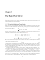
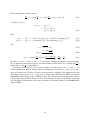
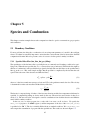
First, we present qualitative results for the case in which ν = 0. Thus, only the advective discretization
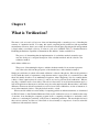
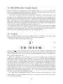
and the time integration are being tested. Figure 3.1 shows the initial and final (t = 2π) numerical solution
for the case N = 64. As mentioned, with ν = 0 the solution is periodic in time and this figure demonstrates
that, as should be the case, the FDS numerical solution is unaltered after one flow-through time.
11
Figure 3.1: Initial and final states of the u-component of velocity.
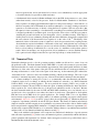
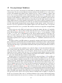
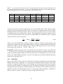
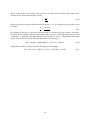
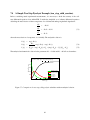
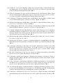
Next, in Figure 3.2, we show time histories of the u-component of velocity at the center of the domain for
the case in which ν = 0.1. It is clearly seen that the FDS solution (thin line) converges to the analytical solution (thick line). Note that the analytical solution is evaluated at the same location as the FDS staggered grid
location for the u-component of velocity, (xN/2 , ȳN/2 ), which is different in each case, N = {8, 16, 32, 64}.
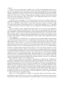
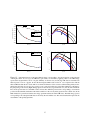
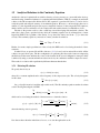
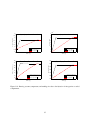
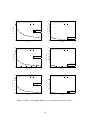
Figure 3.3 is the key quantitative result of this verification test. In this figure we plot the rms error, εrms ,
in the u-component of velocity against the grid spacing. The error is defined by
s
i2
1 M h k
εrms ≡
Ui j − u(xi , ȳ j ,tk ) ,
(3.6)
∑
M k=1
where M is the number of time steps and k is the time step index. The spatial indices are (i = N/2, j = N/2)
and Uikj represents the FDS value for the u-component of velocity at the staggered storage location for cell
(i, j) at time step k; u(xi , ȳ j ,tk ) is the analytical solution for the u-component at the corresponding location
in space and time. The figure confirms that the advective terms, the viscous terms, and the time integration
in the FDS code are convergent and second-order accurate.
12
ns2d 8 nupt1
ns2d 16 nupt1
Analytical (u-vel)
FDS (UVEL)
2
Velocity (m/s)
Velocity (m/s)
2
1.5
1
0.5
0
1
2
3
4
Time (s)
5
6
7
1
0
1
2
3
4
Time (s)
ns2d 64 nupt1
Analytical (u-vel)
FDS (UVEL)
5
6
7
Analytical (u-vel)
FDS (UVEL)
2
Velocity (m/s)
2
Velocity (m/s)
1.5
0.5
ns2d 32 nupt1
1.5
1
0.5
0
Analytical (u-vel)
FDS (UVEL)
1.5
1
0.5
1
2
3
4
Time (s)
5
6
7
0
1
2
3
4
Time (s)
5
6
7
Figure 3.2: Time history of the u-component of velocity half a grid cell below the center of the domain for a
range of grid resolutions. The domain is a square of side L = 2π m. The N × N grid is uniform. Progressing
from left to right and top to bottom we have resolutions N = {8, 16, 32, 64} clearly showing convergence
of the FDS numerical solution (open circles) to the analytical solution (solid line). The case is run with
constant properties, ρ = 1 kg/m3 and µ = 0.1 kg/m/s, and a CFL of 0.25.
13
10
10
10
0
0
10
Convergence Study, Inviscid Case
RMS Error (m/s)
RMS Error (m/s)
10
−1
−2
Convergence Study, Viscous Case
−1
10
−2
10
O(δx)
O(δx2 )
FDS (rms error)
−3
−3
10
−1
10
O(δx)
O(δx2 )
FDS (rms error)
−1
10
Grid Spacing, δx (m)
Grid Spacing, δx (m)
Figure 3.3: (Left) Convergence rate for the u-component of velocity with ν = 0 showing that the advective
terms in the FDS code are second-order accurate. The triangles represent the rms error in the u-component
for grid spacings of δx = L/N where L = 2π m and N = {8, 16, 32, 64}. The solid line represents first-order
accuracy and the dashed line represents second-order accuracy. The simulation is run to a time of t = 2π s
with a CFL of 0.25. The u-component at the center of the domain is compared with the analytical solution
at the same location. (Right) Same case, except ν = 0.1, showing that the viscous terms in the FDS code are
second-order accurate.
14
3.2
Decaying Isotropic Turbulence
In this section we present a canonical flow for LES which tests whether the subgrid stress model has been
coded properly. In some cases the difference between verification and validation is not so clear. Once a
model is well-established and validated it may actually be used as a form of verification. Granted, such
a test is not as strong a verification as the convergence study shown in Section 3.1. Nevertheless, these
tests are often quite useful in discovering problems within the code. The case we examine in this section,
decaying isotropic turbulence, is highly sensitive to errors in the advective and diffusive terms because the
underlying physics is inherently three-dimensional and getting the problem right depends strongly on a
delicate balance between vorticity dynamics and dissipation. An even more subtle yet extremely powerful
verification test is also presented in this section when we set both the molecular and turbulent viscosities to
zero and confirm that the integrated kinetic energy within the domain remains constant. In the absence of
any form of viscosity, experience has shown that the slightest error in the advective terms or the pressure
projection will cause the code to go unstable. This verification is therefore stronger than one might initially
expect.
In this section we test the FDS model against the low Reynolds number (Re) data of Comte-Bellot
and Corrsin (CBC) [38]. Viscous effects are important in this data set for a well-resolved LES, testing the
model’s Re dependence. Following [39], we use a periodic box of side L = 9 × 2π centimeters (≈ 0.566
m) and ν = 1.5 × 10⁻⁵ m2 /s for the kinematic viscosity. The non-dimensional times for this data set are:
x/M = 42 (initial condition), 98, and 171, where M is the characteristic mesh spacing of the CBC wind
tunnel and x is the downstream location of the data station. Considering the mean velocity in the CBC
wind tunnel experiment, these correspond to dimensional times of t = 0.00, 0.28, and 0.66 seconds in our
simulations.
The initial condition for the FDS simulation is generated by superimposing Fourier modes with random
phases such that the spectrum matches that of the initial CBC data. An iterative procedure is employed where
the field is allowed to decay for small time increments subject to Navier-Stokes physics, each wavenumber
is then injected with energy to again match the initial filtered CBC spectrum. The specific filter used here is
discussed in [40].
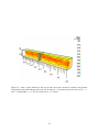
To provide the reader with a qualitative sense of the flow, Figure 3.4 shows the initial and final states
of the velocity field in the 3D periodic domain. The flow is unforced and so if viscosity is present the
total energy decays with time due to viscous dissipation. Because the viscous scales are unresolved, a
subgrid stress model is required. Here the stress is closed using the gradient diffusion hypothesis and the
eddy viscosity is modeled by the constant coefficient Smagorinsky model with the coefficient taken to be
Cs = 0.2 (see the Technical Reference Guide for further details).
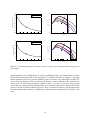
The decay curves for two grid resolutions are shown plotted on the left in Figure 3.5. For an LES code
such as FDS which uses a physically-based subgrid model, an important verification test is to run this periodic isotropic turbulence simulation in the absence of both molecular and turbulent viscosity. For so-called
“energy-conserving” explicit numerics the integrated energy will remain nearly constant in time. This is
demonstrated by the blue line in the top-left plot in Figure 3.5. The deviations from identical energy conservation (to machine precision) are due solely to the time discretization (the spatial terms are conservative as
discussed in [41]) and converge to zero as the time step goes to the zero. Note that strict energy conservation requires implicit time integration [42, 43] and, as shown by the red curve on the same plot where only
molecular viscosity is present in the simulation, this cost is unwarranted given that the molecular dissipation
rate clearly overshadows the relatively insignificant amount of numerical dissipation caused by the explicit
method. The FDS result using the Smagorinsky eddy viscosity (the black solid line) matches the CBC data
(red open circles) well for the 323 case (top-left). However, the FDS results are slightly too dissipative in
the 643 case (bottom-left). This is due to a well-known limitation of the constant coefficient Smagorinsky
model: namely, that the eddy viscosity does not converge to zero at the appropriate rate as the filter width
15
Figure 3.4: Initial and final states of the isotropic turbulence field.
(here equivalent to the grid spacing) is decreased.
To the right of each decay curve plot in Figure 3.5 is the corresponding spectral data comparison. The
three black solid lines are the CBC spectral data for the points in time corresponding to dimensional times
of t = 0.00, 0.28, and 0.66 seconds in our simulations. As described above, the initial FDS velocity field
(represented by the black dots) is specified to match the CBC data up to the grid Nyquist limit. From there
the spectral energy decays rapidly as discussed in [40]. For each of the spectral plots on the right, the results
of interest are the values of the red and blue dots and how well these match up with the corresponding CBC
data. For the 323 case (top-right) the results are remarkably good. Interestingly, the results for the more
highly resolved 643 case are not as good. This is because the viscous scales are rather well-resolved at the
later times in the experiment and, as mentioned, it is well-known that the constant coefficient Smagorinsky
model is too dissipative under such conditions.
Overall, the agreement between the FDS simulations and the CBC data is satisfactory and any discrepancies can be explained by limitations of the model. Therefore, as a verification the results here are positive
in that nothing points to coding errors.
16
−3
0.05
10
Time
0.04
−4
0.035
E(k), m3/s2
kinetic energy (m2/s2)
0.045
FDS zero visc
FDS mol visc
FDS Smag
filtered CBC data
0.03
0.025
0.02
10
−5
10
0.015
0.01
0.005
0
−6
0.1
0.2
0.3
0.4
0.5
0.6
10
0.7
1
10
time (s)
3
10
−3
0.07
10
FDS Smag
filtered CBC data
0.06
Time
0.05
−4
E(k), m3/s2
kinetic energy (m2/s2)
2
10
k, 1/m
0.04
0.03
10
−5
10
0.02
0.01
0
0
−6
0.1
0.2
0.3
0.4
0.5
0.6
10
0.7
1
10
time (s)
2
10
3
10
k, 1/m
Figure 3.5: (Left) Time histories of integrated kinetic energy corresponding to the grid resolutions on the right side
of the figure. In the 323 case (top), the CBC data (open circles) are obtained by applying a filter to the CBC energy
spectra at the Nyquist limit for an N = 32 grid. Similarly, for the 643 case (bottom), the CBC data are obtained from
filtered spectra for an N = 64 grid. Notice that the integrated FDS results for the 323 case compare better with the
filtered CBC data than the 643 results. This is a well-known limitation of the constant coefficient Smagorinsky model:
namely, that the eddy viscosity does not converge to zero at the appropriate rate as the filter width (here equivalent to
the grid spacing) is decreased. (Right) Energy spectra for the 323 case (top) and the 643 case (bottom). The solid black
lines are the spectral data of Comte-Bellot and Corrsin at three different points in time corresponding to downstream
positions in the turbulent wind tunnel. The initial condition for the velocity field (spectra shown as black dots) in the
FDS simulation is prescribed such that the energy spectrum matches the initial CBC data. The FDS energy spectra
corresponding to the subsequent CBC data are shown by the red and blue dots. The vertical dashed line represents the
wavenumber of the grid Nyquist limit.
17
Figure 3.6: Smagorinsky coefficient for a 643 simulation of the CBC experiment.
3.3
The Dynamic Smagorinsky Model
In the previous section, all calculations were performed with a constant and uniform Smagorinsky coefficient, Cs = 0.2. For the canonical case of homogeneous decaying isotropic turbulence – at sufficiently high
Reynolds number – this model is sufficient. However, we noticed that, even for the isotropic turbulence
problem, when the grid Reynolds number is low (i.e., the flow is well-resolved) the constant coefficient
model tends to over predict the dissipation of kinetic energy (see Figure 3.5). This is because the eddy
viscosity does not converge to zero at the proper rate; so long as strain is present in the flow (the magnitude
of the stain rate tensor is nonzero), the eddy viscosity will be nonzero. This violates a guiding principle in
LES development: that the method should converge to a DNS if the flow field is sufficiently resolved [44].
The dynamic procedure for calculating the model coefficient (invoked by setting DYNSMAG=.TRUE.
on the MISC line) alleviates this problem. The basis of the model is that the coefficient should be the same
for two different filter scales within the inertial subrange. Details of the procedure are explained in the
following references [45, 46, 47, 48, 49]. Here we present results for the implementation of the dynamic
model in FDS. In Figure 3.6 we show contours of the Smagorinsky coefficient Cs (x,t) at a time midway
through a 643 simulation of the CBC experiment. Notice that the coefficient ranges from 0.00 to roughly
0.30 within the domain with the average value falling around 0.17.
Next, in Figure 3.7, we show results for the dynamic model analogous to Figure 3.5. For the 323 case the
result is not dramatically different than the constant coefficient model. In fact, one might argue that the 323
constant coefficient results are slightly better. But there are several reasons why we should not stop here and
conclude that the constant coefficient model is superior. First, as pointed out in Pope Exercise 13.34 [50],
383 is required to resolve 80% of the total kinetic energy (for this flow) and thus put the cutoff wavenumber
within the inertial subrange of turbulent length scales. Pope recommends that simulations which are underresolved by this criterion should be termed “very large-eddy simulations” – weather forecasting is a typical
example. For a 323 LES, the test filter width in the dynamic model falls at a resolution of 163 , clearly
outside the inertial range. A tacit assumption underlying the original interpretation of the dynamic model
is that both the grid filter scale and the test filter scale should fall within the inertial range, since this is the
18
−3
0.05
10
FDS Smag
filtered CBC data
Time
0.04
−4
0.035
E(k), m3/s2
kinetic energy (m2/s2)
0.045
0.03
0.025
0.02
10
−5
10
0.015
0.01
0.005
0
−6
0.1
0.2
0.3
0.4
0.5
0.6
10
0.7
1
10
time (s)
3
10
−3
0.07
10
FDS Smag
filtered CBC data
0.06
Time
0.05
−4
E(k), m3/s2
kinetic energy (m2/s2)
2
10
k, 1/m
0.04
0.03
10
−5
10
0.02
0.01
0
0
−6
0.1
0.2
0.3
0.4
0.5
0.6
10
0.7
1
10
time (s)
2
10
3
10
k, 1/m
Figure 3.7: Dynamic Smagorinsky model results (analogous to Figure 3.5) for integrated kinetic energy (left) and
spectra (right).
range in which the scales of turbulent motion (in theory) exhibit fractal-like, scale similar behavior (recently
the procedure has been derived from other arguments [51]). With this in mind, it is perhaps not surprising
that the dynamic model does not perform optimally for the low resolution case. In the higher resolution 643
case, however, the dynamic model does perform better than the constant coefficient model – and this is the
desired result: we want better performance at higher resolution. As can be seen from the energy spectra
(lower right), the energy near the grid Nyquist limit is more accurately retained by the dynamic model. This
equates to better flow structure with fewer grid cells. Thus, for practical calculations of engineering interest
the small computational overhead of computing the coefficient may be recuperated by a reduction is cell
count.
19
3.4
FDS Wall Flows Part I: Straight Channels
Wall flows are notoriously challenging for large-eddy simulation (LES) [52, 53, 54, 50, 55]. In spite of their
promise and sophistication, practical LES codes are resigned to model the wall shear stress as opposed to
resolving the dynamically important length scales near the wall.
In this work we introduce the Werner and Wengle (WW) wall model [56] and the rough wall log law
from Pope [50] into the NIST Fire Dynamics Simulator (FDS) as a practical first step in developing models
for turbulent flow around complex geometry and over complex terrain. Such models are required in order for
FDS to accurately model, for example, tunnel fires, smoke transport in complex architectures, and wildlandurban interface (WUI) fires [57]. As a minimum requirement, a wall model should accurately reproduce the
mean wall stress for flow in a straight channel. We verify that this is true for FDS by reproducing the Moody
chart, a plot of friction factor versus Reynolds number for pipe flow [58].
The remainder of this section is organized as follows. In Section 3.4.1 we describe the model formulation. Then, in Section 3.4.2, we conduct a verification study of the wall boundary conditions for laminar
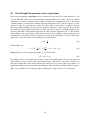
and turbulent flows in FDS. From this study we are able to draw quantitative conclusions in Section 3.4.3
about the accuracy of the channel flow simulations for smooth and rough walls.
3.4.1
Formulation
Details of the FDS formulation are given in the Technical Guide [28]. Here we provide only the salient
components of the model necessary for treatment of constant density channel flow.
The filtered continuity and momentum equations are:
∂ūi
= 0,
∂xi
(3.7)
"
#
sgs
∂ūi ∂ūi ū j
1 dp ∂ p̃ ∂τ̄i j ∂τi j
+
=−
+
+
+
,
∂t
∂x j
ρ dxi ∂xi ∂x j
∂x j
(3.8)
where τsgs
i j ≡ ρ(ui u j − ūi ū j ) is the subgrid-scale (sgs) stress tensor, here modeled by gradient diffusion with
dynamic Smagorinsky [45] used for the eddy viscosity. In this work we specify a constant pressure drop
dp/dx in the streamwise direction to drive the flow. The hyrdrodynamic pressure p̃ is obtained from a
Poisson equation which enforces (3.7).
When (3.8) is integrated over a cell adjacent to a smooth wall in an LES it turns out that the most
difficult term to handle is the viscous stress at the wall, e.g. τ̄xz |z=0 , because the wall-normal gradient of
the streamwise velocity component cannot be resolved. Note that the sgs stress at the wall is identically
zero. We have, therefore, an entirely different situation than exists in the bulk flow at high Reynolds number
where the viscous terms are negligible and the sgs stress is of critical importance. The quality of the sgs
model still influences the wall stress, however, since other components of the sgs tensor affect the value of
the near-wall velocity and hence the resulting viscous stress determined by the wall model. In particular, it
is important that the sgs model is convergent (in the sense that the LES formulation reduces to a DNS as
the filter width becomes small) so that as the grid is refined we can expect more accurate results from the
simulation. For smooth walls the model used for τw = τ̄xz |z=0 in this work is the Werner and Wengle model
[56] which is described in detail in the FDS Tech Guide.
For rough walls the momentum flux normal to the wall is balanced by inviscid drag forces on the
surface elements [59]. In this case FDS models the stress by a rough wall log law (see Pope [50]). Details
are provided in the Tech Guide.
20
0
10
−1
Friction Factor Error
10
−2
10
−3
10
−4
FDS
O(δz)
O(δz 2 )
10
−2
10
−1
Grid Spacing, δz (m)
10
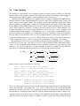
Figure 3.8: FDS exhibits second-order convergence for laminar (Poiseuille) flow in a 2D channel.
3.4.2
Results
Laminar
As verification of the no-slip boundary condition and further verification of the momentum solver in FDS, we
perform a simple 2D laminar (Poiseuille) flow calculation of flow through a straight channel. The height of
the channel is H = 1 m and the length of the channel is L = 8 m. The number of grid cells in the streamwise
direction x is Nx = 8. The number of cells in the wall-normal direction z is varied Nz = {8, 16, 32, 64}. The
fluid density is ρ = 1.2 kg m−3 and the viscosity is 0.025 kg m−1 s−1 . The mean pressure drop is prescribed
to be dp/dx = −1 Pa m−1 resulting in ReH ≈ 160. The (Moody) friction factor f , which satisfies
∆p = f
L1 2
ρū ,
H2
(3.9)
is determined from the steady state mean velocity ū which is output by FDS for the specified pressure drop.
The exact friction factor for this flow is fexact = 24/ReH . The friction factor error | f − fexact | is plotted for
a range of grid spacings δz = H/Nz in Figure 3.8 demonstrating second-order convergence of the laminar
velocity field.
Turbulent
Smooth Walls To verify the WW wall model for turbulent flow we perform 3D LES of a square channel
with periodic boundaries in the streamwise direction and a constant and uniform mean pressure gradient
driving the flow. The problem set up is nearly identical to the laminar cases of the previous section except
here we perform 3D calculations and maintain cubic cells as we refine the grid: we hold the ratio 8:1:1
between Nx :Ny :Nz for all cases. The cases shown below are identified by their grid resolution in the z
direction. The velocity field is initially at rest and develops in time to a mean steady state driven by the
specified mean pressure gradient. The presence of a steady state is the result of a balance between the
21
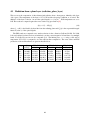
Table 3.1: Case matrix and friction factor results for turbulent channel flow with smooth walls. The height of the
first grid cell δz is given in viscous units z+ for each case. Additionally, the table gives the nominal Reynolds number
ReH and the FDS friction factor results compared to the Colebrook equation (3.10).
dp/dx
(Pa/m)
-0.01
-1.
-100.
Nz = 8
190
1.9 × 10³
1.9 × 10⁴
z+
Nz = 16
95
950
9.5 × 10³
ReH
Nz = 32
47
470
4.7 × 10³
5.9 × 10⁴
7.5 × 10⁵
9.8 × 10⁶
f FDS
(Nz = 32)
0.0212
0.0128
0.0077
f Colebrook
Eq. (3.10)
0.0202
0.0122
0.0081
rel. error
%
4.8
4.6
6.0
streamwise pressure drop and the integrated wall stress from the WW model. FDS outputs the planar
average velocity in the streamwise direction and once a steady state is reached this value is used to compute
the Reynolds number and the friction factor. Table 3.1 provides a case matrix: nine cases for three values
of specified pressure drop and three grid resolutions. The nominal Reynolds number (obtained post-run)
is listed along with the friction factor from the most refined FDS case and the friction factor computed
(iteratively) from the Colebrook equation,
1
z /H
2.51
√ = −2.0 log10 0
√
,
(3.10)
+
3.7
f
ReH f
which is a fit to the turbulent range of the Moody chart (for example, see Ref. [60]). The parameter z0 /H
is the relative roughness where H is the hydraulic diameter of the pipe or channel and ReH is the Reynolds
number based on H. To provide a qualitative picture of the flow field, Figure 3.9 shows contours of streamwise velocity for the case dp/dx = −1 Pa m−1 and Nz = 32.
Rough Walls With the same grid set up as described above the smooth walls, a series of cases labeled as
z0* in the repository were run at various roughness heights, grid resolutions, and Reynolds numbers. The
results are presented together with the smooth wall cases in Fig. 3.10. The laminar cases provide accurate
results for two different Reynolds numbers. As can bee seen, both the smooth wall and rough wall treatments
behave well over the range tested.
3.4.3
Conclusions
In this work the FDS wall model has been verified for both laminar and turbulent flow through straight
channels with smooth or rough walls. It is shown that for the laminar (DNS) case FDS is second-order
accurate. It is suggested elsewhere that, as a rule of thumb, 10 % accuracy is the best that can be expected
from friction factor calculations of turbulent flow [60]. The Werner and Wengle wall model is adapted to
variable density flows (though only constant density flows are tested here) for smooth walls and it is shown
that FDS is capable of reproducing friction factors for a broad range of Reynolds numbers to within 6.0 %
relative accuracy. A log law for rough walls is adopted to FDS with similar results.
22
Figure 3.9: LES of square channel flow with smooth walls and periodic streamwise boundaries using dynamic
Smagorinsky and the Werner Wengle wall model. For this image Nz = 32 and the mean pressure drop is dp/dx = −1
Pa m−1 resulting in ReH = 7.5 × 10⁵ and a friction factor of f = 0.0128.
23
z0 /H
0.1
−1
10
0.01
f
0.001
−2
2
10
0.0001
= 8, H = 1
= 16, H = 1
= 32, H = 1
= 16, H = 2
Nz
Nz
Nz
Nz
10
3
10
4
10
5
10
ReH
6
10
7
10
8
10
Figure 3.10: The FDS Moody Chart: friction factor, f , versus Reynolds number, Re. The solid line for Re < 2000 is
the analytical result for 2D Poiseuille flow, f = 24/Re. The solid lines for Re > 2000 (from the Colebrook equation
(3.10)) are for turbulent flow at various levels of relative roughness z0 /H shown on the right axis. Stars are DNS results
from FDS at a single grid resolution (Nz = 64). Symbols are FDS results for 3D LES with dynamic Smagorinsky. Black
symbols show results for the Werner Wengle wall model at three grid resolutions (Nz = {8, 16, 32}). Colored symbols
are FDS results for the rough wall cases at different grid resolutions and relative roughnesses as differentiated by the
symbol shapes.
24
3.5
Analytical Solutions to the Continuity Equation
Analytical solutions for primitive flow variables (density, velocity, pressure, etc.) are useful in the development and testing of numerical schemes for computational fluid dynamics (CFD). For example, an analytical
solution to the 2D incompressible Navier-Stokes (NS) equations is presented in Section 3.1 and is used to
verify the spatial and temporal accuracy of momentum equation. However, to our knowledge, there are no
similar (i.e., time dependent and periodic in space) analytical solutions for the compressible NS equations,
which could be used for verification of both compressible and variable-density low-Mach flow solvers.
The aim of the present work is to take a small step toward developing such analytical solutions. The
main idea is that, given a specified velocity field, the continuity equation can be rearranged into a linear
hyperbolic PDE for the logarithm of the density. Let ρ denote the density and let u = [u, v]T denote the
velocity. The continuity equation (conservation of mass) can then be written as
∂ ln ρ
+ u · ∇ ln ρ + ∇ · u = 0 .
∂t
(3.11)
Further, for certain, simple specifications of the velocity, this PDE can be solved using the method of characteristics.
In what follows we present 1D and 2D solutions to (3.11) for two basic irrotational flow fields. All the
solutions are periodic in space. The first configuration is a pulsating flow that cycles between compressing
the fluid toward the center and then the corners of the domain. In the second configuration, time periodicity
is achieved by using a constant and uniform advection velocity in combination with the compression waves.
This results in a solution with a qualitatively different character than the first.
3.5.1
Pulsating 1D solution
We specify the velocity as
u(x,t) = B sin(x) cos(ωt) ,
(3.12)
where B is a constant amplitude and ω is the frequency of the compression cycle. The velocity divergence
in 1D is then
∂u
= B cos(x) cos(ωt) .
(3.13)
∂x
Let q ≡ ln ρ (this notation is used through out this work). The 1D continuity equation can then be written
as the following linear hyperbolic PDE:
∂q
∂q
+ B sin(x) cos(ωt) + B cos(x) cos(ωt) = 0 ,
∂t
∂x
which can be solved using the method of characteristics to obtain the solution
2B
1 + tan2 x0 [x,t]
B
exp
sin[ωt]
2
ω
q(x,t) = q(x0 [x,t], 0) + ln
− sin(ωt) ,
ω
1 + tan2 x0 [x,t]
2
(3.14)
(3.15)
where the initial position is given by
h i
x
B
x0 (x,t) = 2 arctan tan
exp − sin(ωt) .
2
ω
Note that we have taken the initial time to be zero, as is done throughout this work.
25
(3.16)
3.5.2
Pulsating 2D solution
There is a simple extension of the 1D stationary wave solution to 2D. In this section we consider the velocity
field u = [u, v]T with components and velocity divergence given by
u(x,t) = B sin(x) cos(ωt) ,
(3.17)
v(y,t) = B sin(y) cos(ωt) ,
(3.18)
∇ · u = B(cos[x] + cos[y]) cos(ωt) ,
(3.19)
∂q
∂q
∂q
+ B sin(x) cos(ωt) + B sin(y) cos(ωt) + B(cos[x] + cos[y]) cos(ωt) = 0 ,
∂t
∂x
∂y
(3.20)
where, again, B is a constant amplitude and ω is the compression frequency. The 2D continuity equation
may then be written as
where, again, q ≡ ln ρ(x,t).
The solution to (3.20) can be obtained by adding the solutions of the following two PDEs:
∂q1
∂q1
+ B sin(x) cos(ωt)
+ B cos(x) cos(ωt) = 0 ,
∂t
∂x
∂q2
∂q2
+ B sin(y) cos(ωt)
+ B cos(y) cos(ωt) = 0 .
∂t
∂y
(3.21)
(3.22)
Thus, utilizing (3.15) and (3.16), and replacing q1 (x0 [x,t], 0) + q2 (y0 [y,t], 0) with q0 (x, y,t), we find that the
solution to (3.20) is
q(x, y,t) = q0 (x, y,t)
(
)
1 + a(x0 [x,t]) exp 2B
ω sin[ωt]
+ ln
1 + a(x0 [x,t])
(
)
1 + a(y0 [y,t]) exp 2B
ω sin[ωt]
+ ln
1 + a(y0 [y,t])
−
2B
sin(ωt) ,
ω
where
a(z) ≡ tan2
(3.23)
z
2
,
(3.24)
and the initial positions are given by
h i
x
B
x0 (x,t) = 2 arctan tan
exp − sin(ωt) ,
2
ω
h i
y
B
y0 (y,t) = 2 arctan tan
exp − sin(ωt) .
2
ω
(3.25)
(3.26)
∂q0
0
Note that the initial condition q0 (x, y,t) is restricted to cases where ∂q
∂x is independent of y and ∂y is independent of x. That is, the function q0 must be additively separable.
An example of the solution to (3.23) is shown in Figure 3.11. The initial condition for the density is
specified as ρ(x, 0) = 1 and the amplitude and frequency are set to unity, B = 1 and ω = 1. FDS is run with
three scalar transport schemes: central differencing, Superbee, and the CHARM flux limiter. The solution
at (x, y) = (3π/2, 3π/2) for successively finer grid resolutions is plotted as a time series on the left and may
be compared with the analytical solution (black line). On the right, we confirm second-order convergence
for the FDS implementation. Central differencing and the CHARM limiter outperform Superbee for this
problem because the solution is relatively smooth.
26
−1
10
FDS N=16
FDS N=32
FDS N=64
FDS N=128
Analytical Solution
1.5
FDS Central
FDS Superbee
FDS CHARM
O(δx)
O(δx2 )
−2
10
L2 Error (kg/m3 )
Density (kg/m3 )
2
1
0.5
−3
10
−4
10
−5
10
0
0
−6
2
4
6
Time (s)
8
10
10
12
−2
10
−1
10
Grid Spacing, δx (m)
0
10
Figure 3.11: (Left) Time series of ρ at the position (x, y) = (3π/2, 3π/2) for several grid resolutions using the
Superbee limiter. (Right) Convergence plot for central differencing, Superbee, and CHARM. All schemes
are second-order accurate.
3.5.3
Stationary compression wave in 1D
Another problem which can be solved analytically is that of a stationary compression wave. In this section
we consider a stationary compression wave combined with a constant and uniform advection velocity in 1D.
The velocity is specified to be
u(x) = c + sin(x) ,
(3.27)
where |c| > 1 is a constant. The 1D continuity equation becomes
∂q
∂q
+ [c + sin(x)] + cos(x) = 0 .
∂t
∂x
(3.28)
A solution to (3.28) is
q(x,t) = q(x0 [x,t], 0)
+ ln −c2 − cos bt + 2 arctan[γ(x,t)] + b sin bt + 2 arctan[γ(x,t)]
− ln −c2 − cos 2 arctan[γ(x,t)] + b sin 2 arctan[γ(x,t)] ,
where
p
−1 + c2 > 0 ,
1 + c tan x0 [x,t]
2
γ(x,t) =
,
b
b
1 + c tan[x/2]
bt
1
x0 (x,t) = 2 arctan
tan arctan
−
−
.
c
b
2
c
b≡
and
3.5.4
(3.29)
(3.30)
(3.31)
(3.32)
Stationary compression wave in 2D
As with the pulsating flow, there is a simple extension of the 1D stationary wave solution to 2D. In this
section we consider the velocity field with components
u(x) = c1 + sin(x) ,
(3.33)
v(y) = c2 + sin(y) .
(3.34)
27
The continuity equation can be written as
∂q
∂q
∂q
+ [c1 + sin(x)] + [c2 + sin(y)] + cos(x) + cos(y) = 0 .
∂t
∂x
∂y
(3.35)
A solution to (3.35) is
q(x, y,t) = q0 (x, y,t)
+ I1 (x,t) − I10 (x,t)
+ I2 (y,t) − I20 (y,t) ,
(3.36)
where
Ii (z,t) = ln −c2i − cos bit + 2 arctan[γi (z,t)] + bi sin bit + 2 arctan[γi (z,t)]
Ii0 (z,t) = ln −c2i − cos 2 arctan[γi (z,t)] + bi sin 2 arctan[γi (z,t)] ,
and
q
bi ≡ −1 + c2i > 0 ,
1 + ci tan z0 [z,t]
2
γi (z,t) =
,
bi
bit
1
bi
1 + ci tan[z/2]
z0 (z,t) = 2 arctan
tan arctan
−
−
.
ci
bi
2
ci
,
(3.37)
(3.38)
(3.39)
(3.40)
(3.41)
Note that z0 ⇒ x0 for i = 1 and z0 ⇒ y0 for i = 2. To be clear, no summation is implied over repeated indices.
0
Also, note that the same restrictions apply to the initial condition as did in Section 3.5.2. Namely, that ∂q
∂x is
0
independent of y and ∂q
∂y is independent of x.
An example of the solution to (3.36) is shown in Figure 3.12. In this case we set c1 = 2 and c2 = 3 to
create an asymmetry in the flow. The periodicity in time depends on the choices of c1 and c2 ; it is possible
that no periodicity exists. We have not found a case that generates a singularity. The analytical time series
of the density at the position (x, y) = (3π/2, 3π/2) is shown as the solid black line. FDS is run with the
CHARM flux limiter scheme (as this is a DNS flow field). The solution at successively finer grid resolutions
is plotted and compared with the analytical solution, demonstrating convergence of the scheme. On the right
side of the figure we demonstrate second-order convergence of the central, Superbee, and CHARM limiter
schemes in FDS.
28
−1
8
6
L2 Error (kg/m3 )
7
Density (kg/m3 )
10
FDS N=16
FDS N=32
FDS N=64
FDS N=128
Analytical Solution
5
4
3
2
FDS Central
FDS Superbee
FDS CHARM
O(δx)
O(δx2 )
−2
10
−3
10
1
0
0
−4
2
4
6
Time (s)
8
10
10
12
−2
10
−1
10
Grid Spacing, δx (m)
0
10
Figure 3.12: (Left) Time series of ρ at the position (x, y) = (3π/2, 3π/2) for several grid resolutions using
the CHARM flux limiter. (Right) Convergence plot for three different scalar transport schemes in FDS:
central, Superbee, and CHARM. All schemes are second-order accurate. In addition, notice that Superbee
gives the lowest error at the coarsest resolution while CHARM gives the lowest error at higher resolution.
This is one reason why Superbee is recommended for LES and CHARM is the default for DNS.
29
3.6
Scalar Transport (move_slug)
In this section we demonstrate the qualitative behavior of the Superbee flux limiter scheme for transport of a
square wave. The diffusivity is set to zero and the advecting velocity is constant and uniform u = [1.0 1.0].
The domain is the unit square with a passive scalar marker initialized to zero everywhere, except for two
‘slugs’ of mass. The first slug is set to unity over the region x × z = [0.125, 0.375] × [0.125, 0.375]. The
second slug is set to 1/2 over the region x × z = [0.500, 0.750] × [0.500, 0.750]. With the scalar bounds set
to [0,1], these slugs demonstrate both the boundedness and TVD (total variation diminishing) behavior of
the transport scheme.
This case also tests two different types of boundary conditions applied in FDS. First, the domain is
periodic and the simulation runs for one flow through time. The scalar slugs therefore ideally arrive back
to their original locations with as little diffusion as possible. Also, the domain is broken into four equally
sized meshes, each with 40 × 40 uniform cells. To increase temporal accuracy and focus on the potential
spacial error, we run the case with a CFL of 0.25. In FDS, we refer to the mesh interface as an ‘interpolated
boundary’.
The results of the test are shown visually in Figure 3.13. The upper-left image shows the initial condition. The black lines indicate the mesh interfaces. To the right of the initial condition we show the first slug
crossing the mesh interfaces without incurring spurious noise. The lower left image shows the final result
for the Superbee limiter. By comparison with a first-order scheme (lower right), this test case confirms that
relatively low levels of diffusion are incurred at both periodic and interpolated boundaries in FDS.
30
Figure 3.13: (Upper left) Initial condition. (Upper right) Superbee solution after 0.175 seconds showing the
scalar slug cleanly passing through the mesh interface. (Lower left) Final result for Superbee after one flow
through time. (Lower right) Result for first-order upwinding after one flow through time, illustrating the
relatively low dissipation of the Superbee scheme. Note that, though the first-order scheme is available as
an option in FDS, it is presented here for comparison purposes only. In practice, the higher order Superbee
scheme is preferred for LES (FDS default).
31
3.7
Energy Conservation (energy_budget)
The examples in this section check that mass and energy are conserved for relatively simple configurations.
3.7.1
The Heat from a Fire (energy_budget)
For the purpose of verifying that the basic FDS algorithm is energy conserving, it is useful to think of a single
compartment as a control volume into which energy is generated by a fire and out of which energy either
flows via openings or is conducted through the walls. If the fire’s heat release rate (HRR) is steady, eventually
the system will reach a quasi-steady state (in an LES calculation, there is never a true “steady state”). Two
simple cases, called energy_budget_adiabatic_walls and energy_budget_cold_walls, illustrate that in the
quasi-steady state, the energy generated by the fire is conserved. For the case with adiabatic walls, a 1200 kW
fire is simulated within a compartment that is 10 m by 10 m by 5 m tall. There is a single door and a single
horizontal vent in the ceiling. The walls are assumed to be adiabatic; that is, there is no net heat flux through
them. Another way to look at it is that the walls are perfect insulators. To simplify the case even further, the
radiation transport algorithm is turned off. It is expected that in this case 1200 kW ought to flow out of the
compartment either via the door or ceiling vent. The plot to the left side of Fig. 3.14 shows both the HRR
and enthalpy flow out of the compartment converging to 1200 kW. During the warm up phase, the enthalpy
flow is less than the HRR because energy is consumed heating up the air within the room.
Next, the same compartment with the same fire is now assumed to have cold (20 ◦ C) walls, and the
radiation is switched back on. After a few minutes of simulation, the net enthalpy outflow is approximately
470 kW and the heat losses to the wall (both radiative and convective) are approximately 730 kW. The plot
is shown on the right hand side of Fig. 3.14.
1400
1400
Energy Budget (adiabatic walls)
Energy Budget (cold walls)
1200
Energy Rate (kW)
Energy Rate (kW)
1200
1000
800
600
Expected (HRR)
Expected (Enthalpy Outflow)
Expected (Wall Loss)
FDS (HRR)
FDS (CONV LOSS)
FDS (COND LOSS)
400
200
0
0
100
200
300
Time (s)
400
1000
800
600
Expected (HRR)
Expected (Enthalpy Outflow)
Expected (Wall Loss)
FDS (HRR)
FDS (CONV LOSS)
FDS (COND LOSS)
400
200
500
0
0
600
100
200
300
Time (s)
400
500
600
Figure 3.14: The Energy Budget for two simple compartment fire simulations.
3.7.2
Gas Injection via an Isentropic Process (isentropic)
This example checks that if nitrogen is added to a sealed compartment with adiabatic (i.e. no heat loss)
walls, that the density, pressure and temperature ought to rise according to the ideal gas law for an isentropic
process:
γ
γ γ−1
p2
ρ2
T2
=
=
(3.42)
p1
ρ1
T1
32
The subscripts 2 and 1 refer to the final and initial state, respectively. Nitrogen is a diatomic gas for which
γ = 1.4. As an additional check, the nitrogen is injected at two different rates such that in case A the injection
occurs in 10 s and in case B the injection occurs in 50 s. The nitrogen is introduced into the domain via
small spheres that do not generate or absorb heat. They do not occupy volume either. They just inject the
nitrogen at a specified rate into the particular grid cell that each occupies.
4
2.5
x 10
Density (isentropic)
Pressure (isentropic)
2
1.3
Pressure (Pa)
Density (kg/m3 )
1.35
1.25
1.2
1.1
0
10
20
30
Time (s)
40
50
1
0.5
Analytical (Density)
FDS (density 1)
FDS (density 2)
1.15
1.5
0
0
60
40
Analytical (Pressure)
FDS (pressure 1)
FDS (pressure 2)
10
20
30
Time (s)
40
50
60
450
Temperature (isentropic)
Enthalpy (isentropic)
Enthalpy (kJ)
Temperature (◦ C)
35
30
25
20
400
Analytical (Temperature)
FDS (temperature 1)
FDS (temperature 2)
15
0
10
20
30
Time (s)
40
50
Analytical (Enthalpy)
FDS (enthalpy 1)
FDS (enthalpy 2)
350
0
60
10
20
30
Time (s)
40
50
60
Figure 3.15: Density, pressure, temperature, and enthalpy rise due to the injection of nitrogen into a sealed
compartment.
3.7.3
Gas Injection via a Non-Isentropic Process (isentropic2)
This example checks that if nitrogen is added via an external vent to a sealed compartment with adiabatic
(i.e. no heat loss) walls, that the density, pressure and temperature ought to rise to the same values regardless
of the time of injection. In the two cases, 0.2 kg of N2 are added to a compartment that is 1 m3 in volume.
In the first case, the injection occurs in 10 s, in the second case in 50 s. The temperature of the gas in both
cases is 500 ◦ C. It is expected that the pressure, p, should rise at the rate:
dp γ puA
=
dt
V
33
(3.43)
where u is the injection velocity and A is the area of the vent. The vent area is 0.04 m2 . The density of the
incoming N2 is found from the Equation of State:
ρ=
Wp
RT
(3.44)
The injection velocity is the mass flux divided by the density, u = ṁ00 /ρ, in which case, the pressure rise can
be written
d p γ ṁ00 R T A
(3.45)
=
dt
WV
Note that the pressure rise is constant. In both the fast and slow injection cases, the pressure is expected to
rise 64282 Pa above ambient. The density and temperature rise are also linear. The density increases from
1.164 kg/m3 to 1.364 kg/m3 . The temperature increases from 20 ◦ C to 135.7 ◦ C. The change in the internal
energy of the system, based on the mass and temperature of the added N2 , is:
∆E = (0.2 kg) × (1.039 kJ/kg/K) × (773.15 K) = 160.7 kJ
(3.46)
Adding in the work due to the pressure yields the change in total enthalpy:
∆H = ∆E +V ∆P = 160.7 kJ + (1 m3 ) × ( 64.3 kJ/m3 ) = 225 kJ
34
(3.47)
4
1.5
Density (isentropic2)
1.4
1.3
1.25
1.2
10
20
30
Time (s)
40
50
3
0
0
60
Analytical (Pressure)
FDS (pressure 1)
FDS (pressure 2)
10
20
30
Time (s)
40
50
60
650
Temperature (isentropic2)
Enthalpy (isentropic2)
600
120
Enthalpy (kJ)
Temperature (◦ C)
4
1
160
100
80
60
Analytical (Temperature)
FDS (temperature 1)
FDS (temperature 2)
40
20
0
5
2
Analytical (Density)
FDS (density 1)
FDS (density 2)
1.15
140
Pressure (isentropic2)
6
1.35
1.1
0
x 10
7
Pressure (Pa)
Density (kg/m3 )
1.45
8
10
20
30
Time (s)
40
50
550
500
450
Analytical (Enthalpy)
FDS (enthalpy 1)
FDS (enthalpy 2)
400
350
0
60
10
20
30
Time (s)
40
50
60
Figure 3.16: Density, pressure, temperature, and enthalpy rise due to the injection of nitrogen into a sealed
compartment.
35
3.8
Checking for Coding Errors (symmetry_test)
This example is a very simple test to determine if there are coding errors in the basic flow solver. A closed
box, 1 m on a side, has 6 injection vents, one centered on each face. Air is pumped into the box at a rate
of 0.5 m/s. Anything that might lead to an asymmetry in the flow field is turned off, for example, gravity,
atmospheric stratification, natural convection, and random noise. The resulting flow field is shown at the
left in Fig. 3.17. On the right are plots of the three components of velocity at equidistant corners of the
enclosure. Ideally, there should be two equal and opposite time histories of the three components. Even the
slightest error in coding will throw this off almost immediately.
1
Component Velocity (symmetry test)
Velocity (m/s)
0.5
0
−0.5
−1
0
10
20
30
Time (s)
40
Figure 3.17: Flow field (left) and velocity component plot (right) for the symmetry_test case.
36
50
Chapter 4
Thermal Radiation
The Radiative Transport Equation (RTE) for an absorbing/emitting and scattering medium is
Z
h
i
σs (x, λ)
Φ(s, s0 ) Iλ (x, s0 ) ds0
s · ∇Iλ (x, s) = − κ(x, λ) + σs (x, λ) Iλ (x, s) + B(x, λ) +
4π
4π
(4.1)
where Iλ (x, s) is the radiation intensity at wavelength λ, s is the direction vector of the intensity, κ(x, λ) and
σs (x, λ) are the local absorption and scattering coefficients, respectively, and B(x, λ) is the emission source
term. The integral on the right hand side describes the in-scattering from other directions. In the case of a
non-scattering gas the RTE becomes
h
i
s · ∇Iλ (x, s) = κ(x, λ) Ib (x) − Iλ (x, s)
(4.2)
where Ib (x) is the source term given by the Planck function (see below).
In practical simulations the spectral (λ) dependence cannot be solved accurately. Instead, the radiation
spectrum is divided into a relatively small number of bands and a separate RTE is derived for each band.
The band specific RTE is
s · ∇In (x, s) = κn (x) [Ib,n (x) − In (x, s)] , n = 1...N
(4.3)
where In is the intensity integrated over the band n, and κn is the appropriate mean absorption coefficient
inside the band. The source term can be written as a fraction of the blackbody radiation
Ib,n = Fn (λmin , λmax ) σ T 4 /π
(4.4)
where σ is the Stefan-Boltzmann constant. The calculation of factors Fn is explained in Ref. [61]. When the
intensities corresponding to the bands are known, the total intensity is calculated by summing over all the
bands
I(x, s) =
N
∑ In (x, s)
(4.5)
n=1
There are numerous examples in the heat transfer literature of exact solutions, for simple configurations
of hot and cold objects, of the radiation transport equation.
37
4.1
Radiation from parallel plate in different co-ordinate systems
(plate_view_factor)
This verification case tests the computation of radiative heat flux from hot surface to a differential, parallel
surface at 1 m distance in different co-ordinate systems. The radiating surface is at 1000 ◦ C temperature and
has emissivity of 1.0. The exact values are calculated using the analycal expressions for the view factors.
Co-ordinates
2D cartesian
3D cartesian
2D cylindrical
Heat flux (kW/m2 )
105.3
81.8
74.1
Radiation source
Infinite plate of width 2 m
Square plate of width 2 m
Circular disk of diameter 2 m
A comparison of exact values and FDS predictions at three diffferent angular resolutions is shown below.
Radiative heat flux (plate view factor)
Radiative heat flux (kW/m2 )
120
110
100
90
80
70
Exact 2D
FDS 2D
Exact cart.
FDS cart.
Exact cyl.
FDS cyl.
60
50
40
20
30
40
50
60
70
80
Number radiation angles
38
90
100
110
4.2
Radiation inside a box (radiation_in_a_box)
This verification case tests the computation of three-dimensional configuration factor Φ inside a cube box
with one hot wall and five cold (0 K) walls. An overview of the test geometry is shown here:
H4
H3
c a
b
(y,z)
dA
H2
H1
c
The configuration factors are calculated at the diagonal of the cold wall opposite to the hot wall. The exact
values of the configuration factor from plane element dA to parallel rectangle H are calculated using the
analytical solution [61]
(y,z)
0.025
0.075
0.125
0.175
0.225
(y,z)
0.275
0.325
0.375
0.425
0.475
ΦHdA
0.1457
0.1603
0.1748
0.1888
0.2018
ΦHdA
0.2135
0.2233
0.2311
0.2364
0.2391
Different variations of the case include the mesh resolution (203 and 1003 cells) and the number of radiation
angles (50, 100, 300, 1000, 2000). The exact and FDS results are shown here:
Incident Heat Flux (radiation box)
Incident Heat Flux (radiation box)
0.3
Heat Flux (kW/m2 )
Heat Flux (kW/m2 )
0.3
0.25
0.2
0.15
Analytical (Phi HdA)
FDS (Flux 20 50)
FDS (Flux 20 100)
FDS (Flux 20 300)
FDS (Flux 20 1000)
FDS (Flux 20 2000)
0.1
0.05
0
0
0.2
0.4
0.6
Position (m)
0.25
0.2
0.15
Analytical (Phi HdA)
FDS (Flux 100 50)
FDS (Flux 100 100)
FDS (Flux 100 300)
FDS (Flux 100 1000)
FDS (Flux 100 2000)
0.1
0.05
0.8
0
0
1
39
0.2
0.4
0.6
Position (m)
0.8
1
4.3
Radiation from a plane layer (radiation_plane_layer)
This case tests the computation of three-dimensional radiation from a homogenous, infinitely wide layer
of hot gases. The temperature of the layer is 1273.15 K and the absorption coefficient, κ, is varied. The
thickness of the layer is fixed at 1 m, and the optical depth is τ = (1 κ) m−1 . Wall temperatures are set to
0 K. The results are compared against the exact solution S(τ) presented in [62]
S(τ) = Sb [1 − 2E3 (τ)]
(4.6)
where Sb = σT 4 is the black-body heat flux from the radiating plane and E3 (τ) is the exponential integral
function (order 3) of the optical depth τ.
The FDS results are computed at two mesh resolutions in the x-direction (I=20 and I=150). For I=20,
both one-band and six-band versions are included to test the correct integration of heat fluxes over multiple
bands. For I=20, 2-D versions are also computed (J=1). The limiting case, τ = ∞, using a solid wall of
temperature 1273.15 K, is computed to test the wall heat flux computation. The exact values and FDS
predictions of the wall heat fluxes are given in the table below.
τ
(m−1 )
0.01
0.1
0.5
1.0
10
∞
S(τ)
(kW/m2 )
2.8970
24.9403
82.9457
116.2891
148.9698
148.9709
FDS (I=20,J=20)
1 band
6 bands
2.9214
2.9104
25.5668
25.4705
83.1353
82.8224
115.4055 114.9710
148.9619 148.4011
147.7533 147.1970
40
FDS (I=20,J=1)
1 band
6 bands
2.8364
2.8257
25.1078
25.0133
84.3719
84.0542
117.8011 117.3576
148.9677 148.4069
147.9426 147.3856
FDS (I=150)
1 band
2.9285
25.7191
84.0311
116.7755
148.9695
147.9419
4.4
Wall Internal Radiation (wall_internal_radiation)
In-depth absorption of thermal radiation in a solid is computed using a two-flux model. In this example, the
accuracy of the two-flux model is tested in the computation of the emissive flux from a homogenous layer
of material (thickness L = 0.1 m) at 1273.15 K temperature, surrounded by an ambient temperature of 10 K.
The absorption coefficient κ is varied to cover a range [0.01, 10] of optical depth τ = κL.
The exact solutions for radiative flux are the analytical solutions of plane layer emission [62]
S(τ) = Sb [1 − 2E3 (τ)]
(4.7)
where Sb = σT 4 is the black-body heat flux from the radiating plane and E3 (τ) is the exponential integral
function (order 3) of optical depth, τ. The exact solutions and FDS results are shown in the table below.
τ
0.01
0.1
0.5
1.0
10.
S(τ)
(kW/m2 )
2.897
24.94
82.95
116.3
149.0
41
FDS
(kW/m2 )
2.950
26.98
93.90
128.4
149.0
4.5
Radiation Emitted by Hot Spheres (hot_spheres)
This case tests the calculation of the radiation heat flux from a collection of hot objects. Within two completely open volumes that are 1 m on a side, hot spheres with a diameter of 1 cm and temperature of 500 ◦ C
are situated within a smaller volume that is 0.5 m on a side. One of the open volumes contains 10 spheres,
the other contains 50,000. The simulation lasts for 10 s. In the first volume, the heat loss is just the sum of
the areas of the spheres multiplied by σT 4 (emissivity is specified as unity in this case). See the upper left
plot in Fig. 4.1. In the second volume, the region is densely packed and it is expected that the collection of
spheres will radiate like a solid cube that is 0.5 m on a side and whose temperature is 500 ◦ C. This is just
under 30 kW, as shown in the upper right of Fig. 4.1. The plot in the lower left of Fig. 4.1 shows the incident
heat flux to a gauge positioned at the center of the densely packed volume. It is expected that this gauge
would register a heat flux of σT 4 = 20.26 kW/m2 . Finally, the plot in the lower right of Fig. 4.1 indicates
the integrated intensity, 4σT 4 = 81.04 kW/m2 .
0
0
Loose Pack Radiation Loss (hot spheres)
−10
Energy Loss (kW)
Energy Loss (kW)
−0.02
−0.04
−0.06
−0.08
Exact (Rad Loss 1)
FDS (rad loss 1)
−0.1
0
2
4
Time (s)
6
8
−20
−30
−40
−50
−60
Exact (Rad Loss 2)
FDS (rad loss 2)
−70
−80
0
10
25
2
4
Time (s)
6
10
Integrated Intensity (hot spheres)
80
Intensity (kW/m2 )
20
15
10
5
60
40
20
Exact (Rad Flux)
FDS (rad flux)
0
0
8
100
Incident Heat Flux (hot spheres)
Heat Flux (kW/m2 )
Tight Pack Radiation Loss (hot spheres)
2
4
Time (s)
6
8
Exact (Intensity)
FDS (UII)
0
0
10
2
4
Time (s)
6
8
10
Figure 4.1: The total heat losses, radiative heat flux, and integrated intensity of a collection of loosely and
densely packed radiating spheres.
42
4.6
Radiation Absorbed by Liquid Droplets (droplet_absorption)
This case tests the conservation of energy that is absorbed by liquid droplets. We want to make sure that the
energy that is taken away from the thermal radiation field is accuratelly converted into increased temperature
of the droplets. Considering the total mass of absorbing droplets, the average droplet temperature T¯d is
increased by the absorbed radiation Q̇r according to the following ODE
mc p
d T¯d
= Q̇r
dt
(4.8)
where m and c p are the total mass and specific heat of the droplets, respectively. Here we have assumed that
the convective heat transfer between the gas and droplets is small. (This is implemented by increasing the
gas phase Prandtl number into a artificially high value.) If the absorbed power remains constant during the
time step, the average droplet temperature in the end should be
T¯d = T0 + dt
Z
Q̇r dV /(mc p )
(4.9)
By setting T0 = 0◦ C, dt = 0.01 s, m = 0.01 kg and c p = 1.0 kJ/kg, the value of T¯d should be equal to
the volumetric integral of Q̇r . The following two plots show comparison of the predicted average droplet
temperature and the analytical value in cartesian and cylindrical co-ordinate systems.
4
Droplet Temperature (droplet absorption cart)
3.5
3.5
3
3
Temperature (◦ C)
Temperature (◦ C)
4
2.5
2
1.5
1
Analytical
FDS (ADT)
0.5
0
0
0.002
0.004
0.006
Time (s)
0.008
Droplet Temperature (droplet absorption cyl)
2.5
2
1.5
1
Analytical
FDS (ADT)
0.5
0
0
0.01
0.002
0.004
0.006
Time (s)
0.008
0.01
Figure 4.2: Conserversion of absorbed thermal radiation energy into increased average droplet temperature.
43
44
Chapter 5
Species and Combustion
This chapter contains examples that test the computations related to species concentrations, gas properties
and combustion.
5.1
Boundary Conditions
For most problems involving fire or combustion, the most important parameter of a model is the total heat
release. It is therefore extremely important to assure that the correct amount of fuel is injected into the FDS
computational domain. Below we present a series of test cases for the species boundary conditions.
5.1.1
Specified Mass Flux (low_flux_hot_gas_filling)
The specification of the fuel mass flux is probably the most commonly used boundary condition for specifying a fire. When the user specifies the HRRPUA (heat release rate per unit area), FDS divides this input by
the heat of combustion for the specified fuel (propane by default) and uses this values as the specified mass
flux ṁ00α at the VENT. This seems simple enough. But the problem is complicated by the fact that the total
species flux is the sum of the advective and diffusive fluxes,
ṁ00α = ρYα un − ρDα
∂Yα
∂n
(5.1)
where un is the face normal mass-average velocity and ∂/∂n is the gradient normal to the face. The velocity
is determined from the total mass flux and the density at the face,
un =
∑α ṁ00α
ρ(Y, T )
(5.2)
The density is computed using old values of the face mass fractions and the face temperature which may be
specified or computed depending on choices made by the user. The new face mass fraction is then set to
satisfy (5.1). The test case below is designed to exercise contributions from both the advective and diffusive
terms in this boundary condition.
In the test case, we inject propane into a cube with 1 m2 vents on all six faces. We specify the
MASS_FLUX of propane to be 0.0001 kg/(m2 s) and the temperature of the face of the VENT (TMP_FRONT)
is specified to be 500 ◦ C. The box is initially filled with air at standard conditions. We DUMP a MASS_FILE
and compare the accumulation of propane with the specified rate. The results are shown in Figure 5.1.
45
0.035
Accumulated Mass (kg)
Low Flux Hot Gas Filling
0.03
0.025
0.02
0.015
0.01
0.005
0
0
Specified
FDS
10
20
30
Time (s)
40
50
60
Figure 5.1: Test of specified mass flux boundary condition for low mass flux and specified temperature
on the face of the VENT. (Left) Image of the domain showing contours of propane mass fraction. (Right)
Comparison of the accumulated mass of propane with the FDS values reported in the _mass file.
5.2
Fractional Effective Dose (FED_Device)
The Fractional Effective Dose index (FED), developed by Purser [63], is a commonly used measure of
human incapasitation due to the combustion gases. The present version of FDS uses only the concentrations
of the gases CO, CO2 , and O2 to calculate the FED value as
FEDtot = FEDCO × HVCO2 + FEDO2
(5.3)
The fraction of an incapacitating dose of CO is calculated as
FEDCO = 4.607 × 10⁻⁷ (CCO )1.036 t
(5.4)
where t is time in seconds and CCO is the CO concentration (ppm). The fraction of an incapacitating dose of
low O2 hypoxia is calculated as
FEDO2 =
t
60 exp [8.13 − 0.54 (20.9 −CO2 )]
(5.5)
where CO2 is the O2 concentration (volume per cent). The hyperventilation factor induced by carbon dioxide
is calculated as
exp(0.1930CCO2 + 2.0004)
HVCO2 =
(5.6)
7.1
where CCO2 is the CO2 concentration (percent).
The FED values were computed from specified constant gas concentrations using an external spreadsheet. The gas concentrations are listed in the following table and the FDS and spreadsheet predictions of
FED values are compared in the figures below.
46
0.1
0.1
FED (O2 depletion)
FED (CO)
0.06
0.06
FED
0.08
FED
0.08
0.04
0.04
0.02
0.02
FED (Spreadsheet)
FDS (FED)
0
0
20
40
60
Time (s)
80
FED (Spreadsheet)
FDS (FED)
0
0
100
FED (CO2+CO)
20
40
60
Time (s)
80
100
FED (All gases)
FED
0.1
FED
0.1
0.05
0.05
FED (Spreadsheet)
FDS (FED)
0
0
20
40
60
Time (s)
80
FED (Spreadsheet)
FDS (FED)
0
0
100
20
40
60
Time (s)
80
Figure 5.2: Comparison of FED index predictions with spreadsheet computations.
47
100
48
Chapter 6
Heat Conduction
This chapter contains examples that test the one-dimensional heat conduction solver in FDS. A one-dimensional
heat conduction equation for the solid phase temperature Ts (x,t) is applied in the direction x pointing into
the solid (the point x = 0 represents the surface)
ρs cs
∂Ts
∂ ∂Ts
= ks
+ q̇000
s
∂t
∂x ∂x
In cylindrical and spherical coordinates, the heat conduction equation is written
∂Ts
∂Ts
1 ∂
∂Ts 1 ∂
000
2 ∂Ts
=
rks
+ q̇s ; ρs cs
= 2
r ks
+ q̇000
ρs cs
s
∂t
r ∂r
∂r
∂t
r ∂r
∂r
(6.1)
(6.2)
FDS offers the user these options, with the assumption that the obstruction is not actually recti-linear, but
rather cylindrical or spherical in shape. This option is useful in describing the behavior of small, complicated
“targets” like cables or heat detection devices.
49
6.1
Simple Heat Conduction Through a Solid Slab (heat_conduction)
Analytical solutions of transient, one-dimensional heat conduction through a slab can be found in Refs. [64]
and [65]. Four cases are examined here. In each, a slab of thickness L = 0.1 m is exposed on one face to
an air temperature of Tg = 120 ◦ C. The other face is insulated (adiabatic). The convective heat transfer from
the gas to the slab is q̇00c = h (Tg − Ts ), where h is constant, and Ts is the slab face temperature. No thermal
radiation is included.
Case
A
B
C
D
k
(W/m/K)
0.1
0.1
1.0
10.0
ρ
(kg/m3 )
100
100
1000
10000
c
(kJ/kg/K)
1
1
1
1
150
150
50
0
0
Slab Temperature (heat conduction b)
Temperature (◦ C)
Temperature (◦ C)
Slab Temperature (heat conduction a)
100
Analytical (Front)
Analytical (4 cm)
Analytical (Back)
FDS (Front)
FDS (4 cm)
FDS (Back)
5
10
15
20
Time (min)
25
100
50
100
150
200
Time (min)
250
300
150
Slab Temperature (heat conduction d)
Temperature (◦ C)
Slab Temperature (heat conduction c)
Temperature (◦ C)
Analytical (Front)
Analytical (4 cm)
Analytical (Back)
FDS (Front)
FDS (4 cm)
FDS (Back)
50
0
0
30
150
100
Analytical (Front)
Analytical (4 cm)
Analytical (Back)
FDS (Front)
FDS (4 cm)
FDS (Back)
50
0
0
Bi
hL/k
100
10
1
0.1
h
(W/m2 /K)
100
10
10
10
100
200
300
400
Time (min)
500
100
50
0
0
600
Analytical (Front)
Analytical (4 cm)
Analytical (Back)
FDS (Front)
FDS (4 cm)
FDS (Back)
200
400
Time (min)
600
Figure 6.1: Comparison of heat conduction calculations with analytical solutions.
50
800
6.2
Temperature-Dependent Thermal Properties (heat_conduction_kc)
This example demonstrates the 1-D heat conduction in cartesian, cylindrical and spherical geometries with
temperature-dependent thermal properties. The cartesian solution was computed using HEATING (version 7.3), a multi-dimensional, finite-difference, general purpose heat transfer model [66]. The cylindrical
and spherical solutions were computed using a commercial finite-element solver, ABAQUS.
The sample of homogenous material is initially at 0 ◦ C and at t > 0 exposed to a gas at 700 ◦ C. A
fixed heat transfer coefficient of 10 W/m2 /K is assumed. The density of the material is 10000 kg/m3 . The
conductivity and specific heat are functions of temperature with the following values: k(0) = 0.10 W/m/K,
k(200) = 0.20 W/m/K, c(0) = 1.0 kJ/kg/K, c(100) = 1.2 kJ/kg/K, c(200) = 1.0 kJ/kg/K. The thickness
(radius) of the sample is 0.01 m. In the cartesian case, the back surface of the material is exposed to a gas at
0 ◦ C. In the figure below, the light colored solid lines are FDS results and the dark lines are the HEATING
results. An example input with cylindrical geometry looks like:
&MATL ID='MAT_1'
EMISSIVITY = 0.0
CONDUCTIVITY_RAMP='K_RAMP'
SPECIFIC_HEAT_RAMP = 'C_RAMP'
DENSITY=10000. /
&RAMP
&RAMP
&RAMP
&RAMP
&RAMP
&RAMP
ID
ID
ID
ID
ID
ID
=
=
=
=
=
=
'K_RAMP'
'K_RAMP'
'K_RAMP'
'C_RAMP'
'C_RAMP'
'C_RAMP'
T=0,
T=100,
T=200,
T=0,
T=100,
T=200,
F=
F=
F=
F=
F=
F=
0.10
0.15
0.20
1.00
1.20
1.00
/
/
/
/
/
/
&SURF ID='SLAB'
STRETCH_FACTOR = 1.0
GEOMETRY = 'CYLINDRICAL'
MATL_ID='MAT_1'
THICKNESS=0.01 /
250
50
Surface Temperature (heat conduction kc)
Back/Inner Temperature (heat conduction kc)
40
Temperature (◦ C)
Temperature (◦ C)
200
150
100
HEATING (cart surf)
ABAQUS (cyl surf)
ABAQUS (sph surf)
FDS (cart front)
FDS (cyl front)
FDS (sph front)
50
0
0
5
10
Time (min)
30
20
HEATING (cart back)
ABAQUS (cyl back)
ABAQUS (sph back)
FDS (cart back)
FDS (cyl back)
FDS (sph back)
10
0
0
15
5
10
Time (min)
Figure 6.2: Comparison of heat conduction calculations with a finite-element model.
51
15
6.3
Simple Thermocouple Model (thermocouples)
This example tests the simple thermocouple model in FDS. It consists of a box whose walls and gas temperatures are fixed at 500 ◦ C. Inside the box are three thermocouples with bead diameters of 1, 2, and 3 mm.
Also included in the box are three “targets” – small solid objects whose surfaces are assumed to be composed of small spheres of the same diameter as the thermocouples. Figure 6.3 compares the temperature
rise of the objects. The thermocouple model is not compared with an analytical solutions. This is simply
a comparison of the thermally-thin thermocouple calculation with the thermally-thick “target” calculation.
Small differences in temperature are due to slightly different flow conditions in different regions of the box,
and numerical error due to node spacing and time step size.
600
Surface Temperature (thermocouples)
Temperature (◦ C)
500
400
300
Thick (Target 1)
Thick (Target 2)
Thick (Target 3)
Thin (TC 1)
Thin (TC 2)
Thin (TC 3)
200
100
0
0
20
40
60
Time (s)
80
100
120
Figure 6.3: Comparison of thermally-thin and thick heat conduction into a small sphere.
52
Chapter 7
Pyrolysis
This chapter tests the routines in FDS that calculate the thermal decomposition of materials. Solid surfaces
can consist of multiple layers, and each layer can consist of multiple material components. Each material
component may undergo several competing reactions, and each of these reactions may produce some other
solid component (residue), gaseous fuel, and/or water vapor.
7.1
Mass conservation of pyrolyzed mass (surf_mass_conservation)
The calculations described in this section check the conservation of mass produced by the pyrolysis algorithm. Parameters describing the geometric configuration of the solid are input via a SURF line, and the
reacting materials are described on respective MATL lines. In the tests, four independent modeling options
are varied:
1. The SURF line can be associated with either a solid surface as designated by a VENT line, or by solid
particles as described by a PART line.
2. The SURF geometry can be either CARTESIAN, CYLINDRICAL, or SPHERICAL.
3. The MATL can be either charring (non-zero NU_RESIDUE) or non-charring.
4. The pyrolysis product can be either the fuel gas defined by the mixture fraction model, or an additional
gas species, defined by a SPEC line.
In all cases, the wall thickness (or radius for cylindrical and spherical geometries) is 0.01 m. The material
density is 360 kg/m3 and the yield of gaseous products for the charring cases is 0.5, i.e. half of the original
mass. For cartesian surfaces, the mass loss per unit area is 1.8 kg/m2 for charring, and 3.6 kg/m2 for noncharring materials. For cylindrical surfaces, the volume per unit surface area is r/2, and thus the mass
loss per unit area is 360(1 − 0.5) × r/2=0.9 kg/m2 for charring, and 1.8 kg/m2 for non-charring materials.
For spherical surfaces, the volume per unit surface area is r/3, and thus the mass loss per unit area is
360(1 − 0.5) × r/3=0.6 kg/m2 for charring, and 1.2 kg/m2 for non-charring materials. On the figures found
on the following pages, the computed results are labeled as follows:
Expected indicates the total mass that has pyrolyzed by the end of the simulation.
Gaseous indicates the instantaneous concentration of pyrolyzed mass integrated over the volume of the
computational domain. It should gradually increase from zero to the “Expected” value.
53
Solid indicates the instantaneous value of the solid surface density integrated over the entire surface area.
For charring materials it should decrease from its initial value (twice the final value) to the final
“Expected” value. For non-charring materials, it should decrease from the “Expected” value to zero.
Fuel Gas is the total burning rate integrated over time. It should increase from zero to the “Expected” value.
7.1.1
Pyrolysis at a Solid Surface
The analytical mass losses are calculated by multiplying the mass per unit area by the VENT area, which
in all cases is 1 m2 . The expected and computed results for charring material are compared in 7.1. The
expected and computed results for non-charring material are compared in 7.2.
54
4
3.5
3
3
2.5
2.5
Mass (kg)
Mass (kg)
3.5
4
surf mass vent char cart fuel
2
1.5
1
0
0
50
100
Time (s)
150
2
1.5
1
Expected
Gaseous
Solid
Gaseous Fuel
0.5
surf mass vent char cart gas
Expected
Gaseous
Solid
0.5
0
0
200
50
100
Time (s)
150
200
2
surf mass vent char cyl fuel
2
surf mass vent char cyl gas
1.5
Mass (kg)
Mass (kg)
1.5
1
0.5
0
0
0.5
Expected
Gaseous
Solid
Gaseous Fuel
20
40
60
Time (s)
80
1
0
0
100
1.5
40
60
Time (s)
80
100
surf mass vent char spher gas
1
Mass (kg)
Mass (kg)
20
1.5
surf mass vent char spher fuel
0.5
0
0
Expected
Gaseous
Solid
1
0.5
Expected
Gaseous
Solid
Gaseous Fuel
20
40
60
Time (s)
80
0
0
100
Expected
Gaseous
Solid
20
40
Time (s)
60
80
Figure 7.1: Comparison of analytical mass change and simulated mass changes for charring surfaces associated with vents.
55
5
5
surf mass vent nonchar cart gas
surf mass vent nonchar cart fuel
4
3
Mass (kg)
Mass (kg)
4
Expected
Gaseous
Solid
Gaseous Fuel
2
1
50
100
Time (s)
150
surf mass vent nonchar cyl fuel
2
Expected
Gaseous
Solid
Gaseous Fuel
1
0.5
100
Time (s)
150
200
surf mass vent nonchar cyl gas
Expected
Gaseous
Solid
1
0.5
0
0
50
Time (s)
100
0
0
150
1.5
50
Time (s)
100
150
1.5
surf mass vent nonchar spher fuel
surf mass vent nonchar spher gas
1
Mass (kg)
Mass (kg)
50
1.5
Mass (kg)
Mass (kg)
2
0
0
200
1.5
Expected
Gaseous
Solid
Gaseous Fuel
0.5
0
0
Expected
Gaseous
Solid
1
0
0
2
3
1
Expected
Gaseous
Solid
0.5
20
40
60
Time (s)
80
0
0
100
20
40
60
Time (s)
80
100
Figure 7.2: Comparison of analytical mass change and simulated mass changes for non-charring surfaces
associated with vents.
56
7.1.2
Pyrolysis of Discrete Particles
For lagrangian particles, the expected values of the mass are obtained by multiplying the material density
by the particle volume by the residue fraction. For cartesian surfaces, the particle area is two times the
product of the parameters LENGTH and WIDTH on the SURF line, both of which are given a value 0.05 m. As
a result, the expected masses for particles with cartesian surfaces are 360(1 − 0.5) × 2δLW = 0.009 kg for
charring, and 0.018 kg for non-charring materials. Note that the half-thickness, δ = 0.01 m, is specified on
the SURF line as THICKNESS. For cylindrical particles, the LENGTH is 0.1 m, and the radius, r (specified via
THICKNESS), is 0.01 m. The expected masses are thus 360(1 − 0.5) × πr2 L = 0.00565 kg for charring, and
0.0113 kg for non-charring materials. For spherical particles, the expected mass is 360(1 − 0.5) × 4πr3 /3 =
7.54 × 10⁻⁴ kg for charring, and 1.51 × 10⁻³ kg for non-charring materials.
The analytical and computed results for charring material are compared in 7.3. The analytical and
computed results for non-charring material are compared in 7.4.
57
0.02
0.02
surf mass part char cart fuel
surf mass part char cart gas
0.015
Mass (kg)
Mass (kg)
0.015
0.01
0.005
0.005
Expected
Gaseous
Solid
0
0
50
100
Time (s)
150
100
Time (s)
150
200
surf mass part char cyl gas
0.012
0.01
Mass (kg)
0.01
0.008
0.006
0.004
0.008
0.006
0.004
Expected
Gaseous
Solid
0.002
0
0
20
40
60
Time (s)
80
0
0
100
20
40
60
Time (s)
80
100
−3
x 10
2
x 10
surf mass part char spher fuel
surf mass part char spher gas
1.5
Mass (kg)
1.5
1
0.5
0
0
Expected
Gaseous
Solid
0.002
−3
Mass (kg)
50
0.014
surf mass part char cyl fuel
0.012
2
Expected
Gaseous
Solid
0
0
200
0.014
Mass (kg)
0.01
1
0.5
Expected
Gaseous
Solid
20
40
60
Time (s)
80
0
0
100
Expected
Gaseous
Solid
20
40
60
Time (s)
80
100
Figure 7.3: Comparison of analytical mass change and simulated mass changes for charring surfaces associated with particles.
58
surf mass part nonchar cart fuel
0.02
0.015
Mass (kg)
0.015
Mass (kg)
surf mass part nonchar cart gas
0.02
Expected
Gaseous
Solid
0.01
0.005
Expected
Gaseous
Solid
0.01
0.005
0
0
20
40
60
Time (s)
80
0
0
100
0.015
Mass (kg)
Mass (kg)
60
Time (s)
80
100
surf mass part nonchar cyl gas
0.01
0.005
0.01
0.005
Expected
Gaseous
Solid
0
0
20
40
60
Time (s)
80
20
40
60
Time (s)
80
100
−3
x 10
2.5
x 10
surf mass part nonchar spher fuel
surf mass part nonchar spher gas
2
Mass (kg)
2
1.5
1
0.5
0
0
Expected
Gaseous
Solid
0
0
100
−3
Mass (kg)
40
0.015
surf mass part nonchar cyl fuel
2.5
20
40
60
Time (s)
80
1
0.5
Expected
Gaseous
Solid
20
1.5
0
0
100
Expected
Gaseous
Solid
20
40
60
Time (s)
80
100
Figure 7.4: Comparison of analytical mass change and simulated mass changes for non-charring surfaces
associated with particles.
59
7.2
Development of surface emissivity (emissivity)
For thermally thick materials, the surface emissivity is computed as a mass-weighted sum of the individual
values of the emissivity in the first condensed phase grid cell. In this verification test, the initial material,
having emissivity of 1.0, is converted to another material, having emissivity of 0.0, at a constant rate of
0.1 s−1 . As a result, the surface emissivity should change linearly from 1.0 to 0.0 in 10 s.
1
Surface Emissivity (emissivity)
Emissivity
0.8
0.6
0.4
0.2
Analytical (Emissivity)
FDS (EMISSIVITY)
0
0
2
4
Time (s)
6
8
10
Figure 7.5: Testing the emissivity of solid materials.
60
7.3
Enthalpy of solid materials (enthalpy)
Consider a thin plate of conductive material that is exposed on one side to an elevated temperature heat
source and exposed on the other to an ambient temperature void. In the thermally-thin limit, the temperature
of the slab is governed by the following equation
dTs q̇00front + q̇00back
=
dt
cs ρs δ
(7.1)
In this example, the initial exposure to the front side of the slab is 3 kW/m2 . The original material (call it A)
undergoes a reaction to form material B. The reaction rate is constant, 0.2 s−1 , which in this case means that
material A disappears in exactly 5 s. This is achieved by setting ns and E to 0 and A to 0.2 in the reaction
rate term:
ρs,A ns
E
r=
(7.2)
A exp −
ρs0
RTs
The density and conductivity of both materials are 30 kg/m3 and 10 W/m/K, respectively. The emissivity of
front and back is 1. The specific heat of material A changes from 1.0 kJ/kg/K to 0.1 kJ/kg/K above 80 ◦ C,
while the specific heat of material B is constant at 1.0 kJ/kg/K. The slab is 1 mm thick.
200
Temperature (◦ C)
Surface Temperature (enthalpy)
150
100
50
Analytical (T slab)
FDS (T slab)
0
0
1
2
Time (s)
3
4
Figure 7.6: Testing the enthalpy of solid materials.
Note that the “analytical” solution is actually a simple numerical integration of the equations above with
a small time step to ensure accuracy. This example tests a number of features, including the reaction rate,
mass weighted specific heats, and radiation boundary conditions. Note that the convective heat transfer has
been turned off, and the correct steady-state temperature is calculated by FDS.
61
7.4
A Simple Two-Step Pyrolysis Example (two_step_solid_reaction)
Before considering actual experimental measurements, it is necessary to check the accuracy of the ordinary differential equation solver within FDS. Consider the simplified set of ordinary differential equations
describing the mass fraction of three components of a solid material undergoing thermal degradation:
dYa
dt
dYb
dt
dYc
dt
= −KabYa
= KabYa − KbcYb
(7.3)
= KbcYa
where the mass fraction of component a is 1 initially. The analytical solution is:
Ya (t) = exp(−Kabt)
Kab
exp(−Kabt) − exp(−Kbct)
Yb (t) =
Kbc − Kab
Yc (t) = [Kab (1 − exp(−Kbct)) + Kbc ∗ (exp(−Kabt) − 1)] /(Kab − Kbc )
(7.4)
(7.5)
The analytical and numerical solution for the parameters Kab = 0.389 and Kbc = 0.262 are shown here:
Solid Density (two step solid reaction)
Mass Fraction
1
0.8
0.6
Analytical (Ya)
Analytical (Yb)
Analytical (Yc)
FDS (Ya)
FDS (Yb)
FDS (Yc)
0.4
0.2
0
0
5
10
15
Time (s)
20
25
30
Figure 7.7: Comparison of a two-step solid pyrolysis calculation with an analytical solution.
62
7.5
Interpreting Bench-Scale Measurements
This section describes a method of deriving and applying the values of the kinetic parameters for the thermal
decomposition of a solid, following the methodology described by Lyon [67].
7.5.1
General Theory
Consider a small sample of solid material that is heated at a relatively slow, constant rate. An example of this
process is thermal gravimetric analysis (TGA). Assume that the solid consists of N material components,
with each component mass fraction denoted by Yi (t). As the solid is heated, each component undergoes
a reaction to form undetermined gases or a single solid residue whose mass fraction is denoted Yr (t) and
whose yield is denoted by νr . The governing equations for the component mass fractions is then:
Ei
dYi
= −Ai Yi exp −
; Yi (0) = Y0,i ; i = 1, N
(7.6)
dt
RT
dYr
dYi
= −νr ∑
; Yr (0) = 0
(7.7)
dt
i dt
In the TGA apparatus, the temperature of the sample is increased linearly in time, dT /dt = β. Because
TGA results are usually expressed as a function of temperature rather than time, it is convenient to rewrite
Eq. (7.6) as:
dYi
Ai
Ei
= − Yi exp −
; Y (T = T0 ) = Y0,i
(7.8)
dT
β
RT
The decomposition rate, −dYi /dt, peaks at a temperature denoted by Tp,i with a value denoted by r p,i . At
this temperature, the second derivative of Yi is zero:
"
#
d 2Yi
Ai dYi
Ei
Ei
Ei
dYi Ai
Ei
Ai
Ei
=−
exp −
− Yi exp −
=−
exp −
−
=0
2
2
dT 2
β dT
RTp,i
β
RTp,i RTp,i
dT β
RTp,i
RTp,i
(7.9)
Next, Eq. (7.8) can be integrated from Y0,i to Yp,i (the value of Yi at the peak), and T0 to Tp,i :
Z
Z Yp,i 0 2
Ai RTp,i
Ai Tp,i
Ei
Ei
dYi
0
=−
exp − 0 dT ≈ −
exp −
(7.10)
Yi0
β T0
RT
β (Ei + 2RTp,i )
RTp,i
Y0,i
Using Eq. (7.9) to eliminate Ai yields:
Yp,i
Ei
=−
≈ −1
ln
Y0,i
Ei + 2RTp,i
(Ei 2RTp,i )
(7.11)
or more simply, Yp,i ≈ Y0,i /e. Now, the activation energy can be evaluated using Eqs. (7.6) and (7.9):
2
2
RTp,i
RTp,i
r p,i
e r p,i
Ei
2 Ai
exp −
=
≈
(7.12)
Ei = RTp,i
β
RTp,i
β Yp,i
β Y0,i
Then Ai can be evaluated directly from Eq. (7.6):
e r p,i
r p,i
Ei
Ei
Ai =
exp
≈
exp
Yp,i
RTp,i
Y0,i
RTp,i
(7.13)
Note that the formulae for Ai and Ei can be evaluated with parameters that are obtained directly by inspection
of the plot of mass loss rate versus temperature. For each peak, the values of Tp,i and r p,i are obvious. The
values of Y0,i can be estimated based on the relative area underneath each peak. The values of Y0,i should
sum to 1.
63
7.5.2
Using Micro-Calorimetry Data (cable_11_mcc)
This section describes a method for interpreting micro-combustion calorimeter (MCC) measurements. The
pyrolysis combustion flow calorimeter (PCFC), developed by Lyon and Walters [68] at the U.S. Federal Aviation Administration (FAA), is a device used to measure the heat generated from the combustion of small
(4 mg to 6 mg) material samples by oxygen depletion calorimetry. Samples are pyrolyzed at a specified heating rate in an anerobic atmosphere (typically N2 ) and the resulting gases are mixed with excess oxygen and
combusted in a separate chamber. The heat release rate from the specimen is obtained from measurements
of the concentration of oxygen in the effluent exiting the combustor as a function of time. The methodology
is the basis for the standard test ASTM D 7309 [69].
The results of PCFC measurements for several multi-conductor control cables are shown in Fig. 7.8.
For each cable, the insulation and jacket material were tested separately, and at least three replicates were
performed for each (only one replicate is shown for each sample). The samples, weighing approximately
5 mg, were cut from the cable jackets and conductor insulation material of each of the cables. These samples
were pyrolyzed in the PCFC at a rate of 1 K/s from 100 ◦ C to 600 ◦ C in a nitrogen atmosphere and the
effluent combusted at 900 ◦ C in a mixture consisting of 20 % O2 and 80 % N2 . The resulting curve shows
the heat release rate of the sample as it was heated, normalized by the mass of the original sample. There are
usually one, two or three noticeable peaks in the curve, corresponding to temperatures where a significant
decomposition reaction occurs. Each peak can be characterized by the maximum value of the heat release
rate (q̇ p,i ), the temperature (Tp,i ), and the relative fraction of the original sample mass that undergoes this
particular reaction (Y0,i ). The area under the curve
Z ∞
q̇(T ) dT = β ∆H 0
(7.14)
0
is the sample heating rate (β) times the energy released per unit mass of the original sample (∆H 0 ). This
latter quantity is related to the more conventional heat of combustion via the relation
∆H =
∆H 0
1 − νr
(7.15)
where νr is the fraction of the original mass that remains as residue. Sometimes this is referred to as the
“char yield.” Note that it is assumed to be the same for all reactions.
The MCC measurement is similar to TGA in that it is possible to derive the kinetic parameters, Ai
and Ei , for the various reactions from the heat release rate curve. As an example of how to work with
MCC data, consider the two plots shown in Fig. 7.8. The solid curves in the figures display the results of
micro-calorimetry measurements for the insulation and jacket material of a multi-conductor control cable
(the number 11 has no particular meaning other than to distinguish it from other cables being studied). The
insulation material exhibits two fairly well-defined peaks, whereas the jacket material exhibits three. Thus,
the insulation material is modeled using two solid components, each undergoing a single-step reaction that
produces fuel gas and a solid residue. The jacket material is modeled using three solid components. The
residue yield for the insulation material is 6 %; for the jacket 49 %, obtained simply by weighing the sample
before and after the micro-calorimetry measurement. It is not known which reaction produces what fraction
of the residue. Rather, it is assumed that each reaction yields the same residue in the same relative amount.
The dashed curves in Fig. 7.8 are the results of FDS simulations of the MCC measurements. To mimic the
sample heating, a very thin sheet comprised of a mixture of the solid components with an insulated backing
is heated at the rate specified in the experiment (1 K/s or 60 K/min, the units needed in FDS). For each
reaction, the kinetic parameters are calculated using the formulae (7.12) and (7.13). The values of Tp,i are
64
800
700
800
Heat Release Rate (cable 11 insulation mcc)
600
HRR (W/g)
HRR (W/g)
600
500
400
Exp (HRR)
FDS (hrrpum)
300
500
300
200
100
100
100
200
300
400
Temperature (◦ C)
500
Exp (HRR)
FDS (hrrpum)
400
200
0
0
Heat Release Rate (cable 11 jacket mcc)
700
0
0
600
100
200
300
400
Temperature (◦ C)
500
600
Figure 7.8: Results of a micro-calorimetry analysis of a sample of cable insulation (left) and jacket material
(right).
obtained directly from the figures. The value of r p,i /Y0,i for the ith reaction can be found from:
q̇ p,i
r p,i = β
∆H 0
;
0
∆H =
Z ∞
q̇(T ) dT
(7.16)
0
where q̇ p,i is the value of the ith heat release rate peak. The values, Y0,i , can be estimated from the relative
area under the curve. Their sum ought to be 1. It is important to check the units of all of these quantities
because the results of these experiments are often presented in different ways depending on the particular
application. A mistake in units can result in values of Ai and/or Ei that will invariably cause spurious results.
The dashed curves in Fig. 7.8 are the results of numerically integrating Eq. (7.6) within FDS for each
material component. A typical input line for FDS that describes a single material component undergoing a
single reaction is given by:
&MATL ID
EMISSIVITY
DENSITY
CONDUCTIVITY
SPECIFIC_HEAT
N_REACTIONS
REFERENCE_TEMPERATURE
REFERENCE_RATE
HEATING_RATE
NU_RESIDUE
RESIDUE
NU_FUEL
HEAT_OF_REACTION
=
=
=
=
=
=
=
=
=
=
=
=
=
'Cable 11 Jacket Component A'
...
...
...
...
1
300.
0.0064
60.
0.49
'char'
0.51
... /
Only the relevant parameters are shown. The other parameters are not relevant in this exercise. Note that
REFERENCE_TEMPERATURE is Tp,i , but in units of ◦ C. REFERENCE_RATE is actually r p,i /Y0,i , in units of
s−1 . HEATING_RATE is β in units of K/min. NU_RESIDUE is νr and NU_FUEL is (1 − νr ). Table 7.1 lists
all of the kinetic parameters for the cable insulation and jacket materials. The peak temperatures are easy
to estimate, and the values of r p,i /Y0,i can be fine-tuned to closely match the data. Note that it is possible to
compute values of Ai and Ei and input them directly into FDS, rather than inputting those listed in the table.
However, the values of Ai and Ei are fairly large numbers and have little meaning in their own.
65
Table 7.1: Parameters used to derive the kinetic constants for cable materials. The heating rate for both is
60 ◦ C/min.
Parameter
Tp,i (◦ C)
r p,i /Y0,i (s−1 )
7.5.3
Insulation, νr =0.06
1
2
355
485
0.0384
0.2426
Jacket, νr =0.49
1
2
3
300
345
450
0.0064 0.3500 0.0156
Using TGA Data (birch_tga)
This is an example of a comparison of a candidate solid phase model with TGA (Thermo-gravimetric Analysis) data. The sample cases called birch_tga_1step_2 and birch_tga_1step_20 simulate two standard TGA
experiments in which small samples of birch wood are heated up slowly at constant rates of 2 ◦ C/min and
20 ◦ C/min, respectively. The model of the wood only involves one reaction that converts virgin wood to char
and fuel gases. There is also a reaction in the simulation that does nothing more than evaporate the small
amount of moisture in the wood. This evaporation is evident in Fig. 7.9 near the temperature of 100 ◦ C.
Exp. 2 K/min
Exp. 20 K/min
FDS 2 K/min
FDS 20 K/min
1
Mass Fraction
0.8
0.6
0.4
0.2
0
0
100
200
300
400
500
Temperature (◦ C)
600
700
800
Figure 7.9: Comparison of a solid phase model of birch wood with TGA data.
66
Chapter 8
Lagrangian Particles
This chapter contains verification cases that test all aspects of particles, droplets, sprays, and so on. Note
that in FDS, lagrangian particles are used for a variety of purposes, not just water droplets.
8.1
Momentum Transfer (particle_drag)
The particle drag test cases consider a 1 m by 1 m by 1 m channel with periodic boundary conditions on the
x-faces and FREE_SLIP walls on y- and z-faces. Static droplets are placed in the center of the channel, one
particle per computational cell, so that they form a surface perpendicular to the flow direction. Gravity is set
to zero. Due to the symmetry of the problem the flow is one dimensional. Assuming that the droplets are of
uniform diameter and the drag coefficient and gas density are constant, the velocity in the channel decays
according to
u0
1 ∑ CD π rd2
u=
; B=
(8.1)
1 + B u0 t
2
V
In the above, V is the volume of the channel, rd is the droplet radius, CD is the droplet drag coefficient, and
u is the gas velocity in the x-direction. The summation is over all N particles. The common parameters used
in all the simulations are
CD = 10, rd = 0.005
The initial velocity, u0 , for each case is listed in Table 8.1. Comparisons of computed and analytical results
are shown in Figure 8.1.
Table 8.1: Parameters used in the particle_drag cases
Case
A
B
C
D
E
F
u0
10
50
100
50
100
150
67
N
16
16
16
1600
1600
1600
12
60
Gas phase velocity (particle drag A)
Gas phase velocity (particle drag D)
50
Velocity (m/s)
Velocity (m/s)
10
8
Analytical
FDS
6
4
2
0
0
40
30
20
10
20
40
60
Time (s)
80
0
0
100
60
1
Time (s)
1.5
2
Gas phase velocity (particle drag E)
100
Velocity (m/s)
50
Velocity (m/s)
0.5
120
Gas phase velocity (particle drag B)
40
Analytical
FDS
30
20
10
0
0
Analytical
FDS
80
60
40
20
10
20
30
Time (s)
40
0
0
50
120
Analytical
FDS
0.5
1
Time (s)
1.5
2
200
Gas phase velocity (particle drag C)
Gas phase velocity (particle drag F)
100
Velocity (m/s)
Velocity (m/s)
150
80
Analytical
FDS
60
40
100
50
20
0
0
5
10
15
Time (s)
20
0
0
25
Analytical
FDS
0.5
1
Time (s)
1.5
Figure 8.1: Outputs of the particle_drag test cases compared with analytical solutions.
68
2
8.2
Water Droplet Evaporation (water_evaporation)
The test case called water_evaporation involves stationary water droplets in a box with dimensions of 1 m
on a side. The walls of the box are assumed adiabatic, meaning that there are no leaks or heat losses. The air
within the box is stirred to maintain uniform conditions. Initially, the air temperature is 20 ◦ C, the median
volumetric diameter of the droplets is 100 µm, the water temperature is 90 ◦ C, and the total mass of water
droplets is 0.2 kg. It is expected that a steady-state will be achieved after about 5 s. Figure 8.2 displays
the average enthalpy, humidity, density, pressure, temperature and mass of water of the gas. The horizontal
lines denote the expected initial and steady-state values, respectively. The plot of enthalpy includes the gas
(reference temperature is 0 K) and the liquid water droplets (reference temperature is 0 ◦ C). The decrease
in the enthalpy of the water droplets should equal the increase in the enthalpy of the gas minus the work
performed due to increasing pressure. It is the internal energy of the system that is conserved. The internal
energy can be expressed in terms of the enthalpy, pressure and density:
e = h−
In differential form:
1
de = dh − d p − p d
ρ
p
ρ
1
= dh − v d p − p dv
ρ
(8.2)
(8.3)
Multiplying by mass and noting that the volume, V , is constant yields:
dE = dH −V d p
(8.4)
The enthalpy decrease of the liquid water droplets is equal to the enthalpy gain of the gas (both expressed
in kJ) minus the pressure increase times the volume in units of kPa and m3 , respectively. Finally, note
that in this example that a water droplet will evaporate until the vapor pressure at the droplet surface is in
equilibrium with the vapor pressure in the surrounding air. Thus, the relative humidity should be equal to
100 %, but since FDS does not currently compute condensation, a slight overshoot is not unexpected.
69
500
120
Enthalpy (water evaporation)
Relative Humidity (water evaporation)
100
Humidity (%)
Enthalpy (kJ)
400
Analytical (h gas)
Analytical (h water)
FDS (h gas)
FDS (h water)
300
200
80
60
40
100
0
0
20
1
2
Time (s)
3
4
0
0
5
1.25
Analytical (Rel. Hum)
FDS (humid)
1
2
Time (s)
3
4
5
30
Density (water evaporation)
Gas Temperature (water evaporation)
Temperature (◦ C)
Density (kg/m3 )
1.24
1.23
1.22
1.21
1.2
1.19
0
25
20
Analytical (dens)
FDS (dens)
1
2
Time (s)
3
4
Analytical (temp)
FDS (Temp)
15
0
5
10
2
Time (s)
3
4
5
0.03
Over Pressure (water evaporation)
Evaporated Mass (water evaporation)
0.025
Mass (kg)
8
Pressure (kPa)
1
6
4
0.02
0.015
0.01
2
0.005
Analytical (pres)
FDS (pres)
0
0
1
2
Time (s)
3
4
0
0
5
Analytical (vapor)
FDS (WATER VAPOR)
1
2
Time (s)
3
Figure 8.2: Output of the test case called water_evaporation.
70
4
5
Bibliography
[1] K.B. McGrattan, S. Hostikka, and J.E. Floyd. Fire Dynamics Simulator (Version 5), User’s Guide.
NIST Special Publication 1019-5, National Institute of Standards and Technology, Gaithersburg, Maryland, October 2007. i
[2] American Society for Testing and Materials, West Conshohocken, Pennsylvania. ASTM E 1355-04,
Standard Guide for Evaluating the Predictive Capabilities of Deterministic Fire Models, 2004. i, 1, 9
[3] W. Mell, K.B. McGrattan, and H. Baum. Numerical Simulation of Combustion in Fire Plumes.
In Twenty-Sixth Symposium (International) on Combustion, pages 1523–1530. Combustion Institute,
Pittsburgh, Pennsylvania, 1996. 3
[4] K.B. McGrattan, H.R. Baum, and R.G. Rehm. Large Eddy Simulations of Smoke Movement. Fire
Safety Journal, 30:161–178, 1998. 3
[5] H.R. Baum, R.G. Rehm, P.D. Barnett, and D.M. Corley. Finite Difference Calculations of Buoyant
Convection in an Enclosure, Part I: The Basic Algorithm. SIAM Journal of Scientific and Statistical
Computing, 4(1):117–135, March 1983. 3
[6] H.R. Baum and R.G. Rehm. Finite Difference Solutions for Internal Waves in Enclosures. SIAM
Journal of Scientific and Statistical Computing, 5(4):958–977, December 1984. 3
[7] H.R. Baum and R.G. Rehm. Calculations of Three Dimensional Buoyant Plumes in Enclosures. Combustion Science and Technology, 40:55–77, 1984. 3
[8] R.G. Rehm, P.D. Barnett, H.R. Baum, and D.M. Corley. Finite Difference Calculations of Buoyant
Convection in an Enclosure: Verification of the Nonlinear Algorithm. Applied Numerical Mathematics,
1:515–529, 1985. 3
[9] K.B. McGrattan, T. Kashiwagi, H.R. Baum, and S.L. Olson. Effects of Ignition and Wind on the
Transition to Flame Spread in a Microgravity Environment. Combustion and Flame, 106:377–391,
1996. 4
[10] T. Kashiwagi, K.B. McGrattan, S.L. Olson, O. Fujita, M. Kikuchi, and K. Ito. Effects of Slow Wind
on Localized Radiative Ignition and Transition to Flame Spread in Microgravity. In Twenty-Sixth
Symposium (International) on Combustion, pages 1345–1352. Combustion Institute, Pittsburgh, Pennsylvania, 1996. 4
[11] W. Mell and T. Kashiwagi. Dimensional Effects on the Transition from Ignition to Flame Spread
in Microgravity. In Twenty-Seventh Symposium (International) on Combustion, pages 2635–2641.
Combustion Institute, Pittsburgh, Pennsylvania, 1998. 4
71
[12] W. Mell, S.L. Olson, and T. Kashiwagi. Flame Spread Along Free Edges of Thermally-Thin Samples in Microgravity. In Twenty-Eighth Symposium (International) on Combustion, pages 2843–2849.
Combustion Institute, Pittsburgh, Pennsylvania, 2000. 4
[13] K. Prasad, Y. Nakamura, S.L. Olson, O. Fujita, K. Nishizawa, K. Ito, and T. Kashiwagi. Effect of Wind
Velocity on Flame Spread in Microgravity. In Twenty-Ninth Symposium (International) on Combustion, pages 2553–2560. Combustion Institute, Pittsburgh, Pennsylvania, 2002. 4
[14] Y. Nakamura, T. Kashiwagi, K.B. McGrattan, and H.R. Baum. Enclosure Effects on Flame Spread
over Solid Fuels in Microgravity. Combustion and Flame, 130:307–321, 2002. 4
[15] W.E. Mell, K.B. McGrattan, and H.R. Baum. g-Jitter Effects on Spherical Diffusion Flames. Microgravity Science and Technology, 15(4):12–30, 2004. 4
[16] A. Mukhopadhyay and I.K. Puri. An Assessment of Stretch Effects on Flame Tip Using the Thin
Flame and Thick Formulations. Combustion and Flame, 133:499–502, 2003. 4
[17] A. Hamins, M. Bundy, I.K. Puri, K.B. McGrattan, and W.C. Park. Suppression of Low Strain Rate
Non-Premixed Flames by an Agent. In Proceedings of the 6th International Microgravity Combustion
Workshop, NASA/CP-2001-210826, pages 101–104. National Aeronautics and Space Administration,
Lewis Research Center, Cleveland, Ohio, May 2001. 4
[18] K.B. McGrattan, R.G. Rehm, and H.R. Baum. Fire-Driven Flows in Enclosures. Journal of Computational Physics, 110(2):285–291, 1994. 4
[19] P. Friday and F. W. Mowrer. Comparison of FDS Model Predictions with FM/SNL Fire Test Data.
NIST GCR 01-810, National Institute of Standards and Technology, Gaithersburg, Maryland, April
2001. 6
[20] A. Bounagui, N. Benichou, C. McCartney, and A. Kashef. Optimizing the Grid Size Used in CFD
Simulations to Evaluate Fire Safety in Houses. In 3rd NRC Symposium on Computational Fluid
Dynamics, High Performance Computing and Virtual Reality, pages 1–8, Ottawa, Ontario, Canada,
December 2003. National Research Council, Canada. 6
[21] R.L. Alpert. SFPE Handbook of Fire Protection Engineering, chapter Ceiling Jet Flows. National Fire
Protection Association, Quincy, Massachusetts, 3rd edition, 2003. 6
[22] A. Bounagui, A. Kashef, and N. Benichou. Simulation of the Dynamics of the Fire for a Section of
the L.H.-La Fontaine Tunnel. IRC-RR- 140, National Research Council Canada, Ottawa, Canada,
K1A0R, September 2003. 6
[23] Y. Xin. Assessment of Fire Dynamics Simulation for Engineering Applications: Grid and Domain
Size Effects. In Proceedings of the Fire Suppression and Detection Research Application Symposium,
Orlando, Florida. National Fire Protection Association, Quincy, Massachusetts, 2004. 6
[24] J.A. Ierardi and J.R. Barnett. A Quantititive Method for Calibrating CFD Model Calculations. In Proceedings of the CIB-CTBUH International Conference on Tall Buildings, pages 507–514. International
Council for Research and Innovation in Building and Construction (CIB), 2003. 6
[25] G. Heskestad. SFPE Handbook of Fire Protection Engineering, chapter Fire Plumes, Flame Height
and Air Entrainment. National Fire Protection Association, Quincy, Massachusetts, 3rd edition, 2002.
6
72
[26] N.M. Petterson. Assessing the feasibility of reducing the grid resolution in fds field modeling. Fire
Engineering Research Report 2002/6, University of Canterbury, Christchurch, New Zealand, March
2002. 6
[27] A. Musser, K. B. McGrattan, and J. Palmer. Evaluation of a Fast, Simplified Computational Fluid
Dynamics Model for Solving Room Airflow Problems. NISTIR 6760, National Institute of Standards
and Technology, Gaithersburg, Maryland, June 2001. 6
[28] K.B. McGrattan, S. Hostikka, J.E. Floyd, H.R. Baum, R.G. Rehm, W.E. Mell, and R. McDermott. Fire
Dynamics Simulator (Version 5), Technical Reference Guide, Volume 1: Mathematical Model. NIST
Special Publication 1018-5, National Institute of Standards and Technology, Gaithersburg, Maryland,
October 2007. 7, 20
[29] W. Zhang, A. Hamer, M. Klassen, D. Carpenter, and R. Roby. Turbulence Statistics in a Fire Room
Model by Large Eddy Simulation. Fire Safety Journal, 37:721–752, 2002. 7
[30] J. Smagorinsky. General Circulation Experiments with the Primitive Equations. I. The Basic Experiment. Monthly Weather Review, 91(3):99–164, March 1963. 7
[31] J.W. Deardorff. Numerical Investigation of Neutral and Unstable Planetary Boundary Layers. Journal
of Atmospheric Sciences, 29:91–115, 1972. 7
[32] M. Germano, U. Piomelli, P. Moin, and W.H. Cabot. A Dynamic Subgrid-Scale Eddy Viscosity Model.
Physics of Fluids A, 3(7):1760–1765, 1991. 7
[33] D.K. Lilly. A Proposed Modification of the Germano Subgrid-Scale Closure Method. Physics of Fluids
A, 4(3):633–635, 1992. 7
[34] J. Hietaniemi, S. Hostikka, and J. Vaari. FDS Simulation of Fire Spread – Comparison of Model
Results with Experimental Data. VTT Working Papers 4, VTT Building and Transport, Espoo, Finland,
2004. 8
[35] C. Lautenberger, G. Rein, and C. Fernandez-Pello. The application of a genetic algorithm to estimate
the material properties for fire modeling from bench-scale fire test data. Fire Safety Journal, 41:204–
214, 2006. 8
[36] J.C. Adams, W.S. Brainerd, J.T. Martin, B.T. Smith, and J.L. Wagener. Fortran 95 Handbook: Complete ISO/ANSI Reference. MIT Press, Cambridge, Massachusetts, 1997. 9
[37] R. McDermott. A nontrivial analytical solution to the 2-d incompressible Navier-Stokes equations.
http://randy.mcdermott.googlepages.com/NS_exact_soln.pdf, 2003. 11
[38] G. Comte-Bellot and S. Corrsin. Simple Eularian time correlation of full- and narrow-band velocity
signals in grid-generated, ‘isotropic’ turbulence. J. Fluid Mech., 48:273–337, 1971. 15
[39] Stephen M. de Bruyn Kops. Numerical simulation of non-premixed turbulent combustion. PhD thesis,
The University of Washington, 1999. 15
[40] R. McDermott, A. Kerstein, R. Schmidt, and P. Smith. Characteristics of 1D spectra in finite-volume
large-eddy simulations with one-dimensional turbulence subgrid closure. In 58th Annual Meeting
of the American Physical Society, Division of Fluid Dynamics, Chicago, Illinois, November 2005.
http://randy.mcdermott.googlepages.com/implied_filter.pdf. 15, 16
73
[41] Y. Morinishi, T. S. Lund, O. V. Vasilyev, and P. Moin. Fully conservative high order finite difference
schemes for incompressible flow. J. Comp. Phys., 143:90–124, 1998. 15
[42] F. E. Ham, F. S. Lien, and A. B. Strong. A fully conservative second-order finite difference scheme for
incompressible flow on non-uniform grids. J. Comp. Phys., 177:117–133, 2002. 15
[43] R. McDermott. Discrete kinetic energy conservation for variable-density flows on staggered grids. In
60th Annual Meeting of the American Physical Society, Division of Fluid Dynamics, Salt Lake City,
Utah, November 2007. http://randy.mcdermott.googlepages.com/aps2007_notes.pdf. 15
[44] R. McDermott and S. B. Pope. A particle formulation for treating differential diffusion in filtered
density function methods. J. Comp. Phys., 226(1):947–993, 2007. 18
[45] M. Germano, U. Piomelli, P. Moin, and W. Cabot. A dynamic subgrid-scale eddy viscosity model.
Phys. Fluids A, 3(7):1760–1765, 1991. 18, 20
[46] M. Pino Martin, U. Piomelli, and G. Candler. Subgrid-scale models for compressible large-eddy
simulation. Theoret. Comput. Fluid Dynamics, 13:361–376, 2000. 18
[47] P. Moin, K. Squires, W. Cabot, and S. Lee. A dynamic subgrid-scale model for compressible turbulence
and scalar transport. Phys. Fluids A, 3(11):2746–2757, 1991. 18
[48] T. S. Lund. On the use of discrete filters for large eddy simulation. Center for Turbulence Research
Annual Research Briefs, 1997. 18
[49] R. McDermott. Variable density formulation of the dynamic smagorinsky model. Unpublished notes
(http://randy.mcdermott.googlepages.com/dynsmag_comp.pdf), 2004. 18
[50] Stephen B. Pope. Turbulent Flows. Cambridge, 2000. 18, 20
[51] S.B. Pope. Ten questions concerning the large-eddy simulation of turbulent flows. New Journal of
Physics, 6:1–24, 2004. 19
[52] J. S. Baggett. Some modeling requirements for wall models in large eddy simulation. Stanford Center
for Turbulence Research Annual Research Briefs, 1997. 20
[53] J. S. Baggett. On the feasibility of merging LES with RANS for the near-wall region of attached
turbulent flows. Stanford Center for Turbulence Research Annual Research Briefs, 1998. 20
[54] W. Cabot. Large-eddy simulations with wall models. Stanford Center for Turbulence Research Annual
Research Briefs, 1995. 20
[55] Pierre Sagaut. Large Eddy Simulation for Incompressible Flows. Springer, 2001. 20
[56] H. Werner and H. Wengle. Large-eddy simulation of turbulent flow over and around a cube in a plate
channel. In 8th Symposium on Turbulent Shear Flows, pages 155–168, 1991. 20
[57] NIST Web Site. http://www.fire.nist.gov/wui. 20
[58] L. F. Moody. Friction factors for pipe flow. Transactions of the ASME, 66, 1944. 20
[59] H. Tennekes and J. L. Lumley. A First Course in Turbulence. MIT Press, 1972. 20
[60] Bruce R. Munson, Donald F. Young, and Theodore H. Okiishi. Fundamentals of Fluid Mechanics.
John Wiley and Sons, 1990. 22
74
[61] R. Siegel and J. R. Howell. Thermal Radiation Heat Transfer. Taylor & Francis, New York, 4th
edition, 2002. 37, 39
[62] Y.B. Zel’dovich and Y.P. Raizer. Physics of shock waves and high-temperature hydrodynamic phenomena. Dover Publications, New York, 2002. Translated from the Russian and then edited by W.D.Hayes
and R.F. Probstein. 40, 41
[63] D.A. Purser. SFPE Handbook of Fire Protection Engineering, chapter Toxicity Assessment of Combustion Products. National Fire Protection Association, Quincy, Massachusetts, 3rd edition, 2002.
46
[64] D. Drysdale. An Introduction to Fire Dynamics. John Wiley and Sons, New York, 2nd edition, 2002.
50
[65] H.S. Carslaw and J.C. Jaegar. Conduction of Heat in Solids. Oxford University Press, 2nd edition,
1959. 50
[66] K.W. Childs. HEATING 7: Multidimensional, Finite-Difference Heat Conduction Analysis Code
System. Technical Report PSR-199, Oak Ridge National Laboratory, Oak Ridge, TN, 1998. 51
[67] R.E. Lyon. Heat Release Kinetics. Fire and Materials, 24:179–186, 2000. 63
[68] R.E. Lyon and R.N. Walters. Pyrolysis Combustion Flow Calorimetry. Journal of Analytical and
Applied Pyrolysis, 71(1):27–46, March 2004. 64
[69] American Society for Testing and Materials, West Conshohocken, Pennsylvania. ASTM D 7309-07,
Standard Test Method for Determining the Flammability Characteristics of Plastics and Other Solid
Materials Using Microscale Combustion Calorimetery, 2007. 64
75