Download User's Guide for Parallel WAQUA/TRIWAQ and for Domain

User’s Guide for Parallel
WAQUA/TRIWAQ and for Domain
Decomposition
User’s Guide for Parallel
WAQUA/TRIWAQ and for Domain
Decomposition
Version number
Maintenance
Copyright
:
:
:
Version 2.20, June 2011
see www.helpdeskwater.nl/waqua
Rijkswaterstaat
Log-sheet
Table 1: Log-Sheet
document version
0.1
1.0
1.1
1.2
date
15-10-1999
14-03-2000
21-06-2000
15-11-2000
2.0
28-11-2001
2.1
2.2
2.3
2.4
2.5
2.7
2.8
2.9
2.10
2.11
22-01-2003
27-03-2003
14-11-2003
14-06-2004
25-03-2005
03-08-2005
20-01-2006
22-09-2006
28-12-2006
18-06-2007
09-01-2008
2.12
2.13
2.14
16-01-2008
14-02-2008
30-07-2009
2.15
07-08-2009
2.16
2.17
2.18
2.19
27-07-2010
24-09-2010
19-10-2010
20-10-2010
2.20
21-06-2011
Version 2.20, June 2011
Changes with respect to the previous version
Layout changes: 2-sided template.
P98044: changed header to comply with norm
DDVERT01: added/modified descriptions with respect to domain decomposition with vertical refinement for triwaq
DDHOR01: added/modified descriptions with respect to domain decomposition with horizontal refinement for waqua
and triwaq;
implemented automatic partitioning of boundary points and
the new definition of enclosures in areas-files, removed description of optimization of partitionings;
allow fine grid interfaces to be slightly wider or narrower than
coarse grid interfaces.
P02015: conversion from Word95 to Word2000
P03007: improvements
P03047: general check (export 2003-02)
DDHV01: combination of horizontal and vertical refinement
M05023: corrections in section 1.7 and section 6.2.1
W04003: Incorporation in the User’s Guide waqua
W06005: implemented dynamic allocation of ibuffr
m282136: replaced PVM by description of MPI
m293245: updated description o process configuration-file
c71236: CDCON removed
c77580: added mapping of subdomains onto hosts in
waqpro.pl; reduced number of runs of Waqpre for DDVERT
c77580: removed old-style enclosures from areas-file
c77580: implemented autom. partitioning of a subdomain
c91768: made EXPERIMENT optional for DDHOR configfile
c91768: added optional directory name in DDHOR configfile
c3256: conversion to LATEX
c3384: added hostmap option Packed (with alias Compact)
c3320: added note for using DDHOR i.c.w. Visipart.
c3256: review of conversion to LATEX: corrections in labels
and figures.
c3395: default method is automatic (orb or strip with communication minimized).
i
User’s Guide for Parallel WAQUA/TRIWAQ and for Domain Decomposition
Preface
This report is the User’s Guide for the Parallel and Domain Decomposition functionality of the
WAQUA/TRIWAQ system. For information about the WAQUA and TRIWAQ programs themselves, the reader is referred to other parts in this WAQUA user’s guide (SIMONA report 92-10).
Domain decomposition allows for vertical refinement in TRIWAQ and for horizontal grid refinement for WAQUA and TRIWAQ. A combination of both methods is also possible.
The report first gives an introduction to parallel computing and domain decomposition, and gives
an overview of the components used in such coupled simulations.
The remainder of this report mainly concentrates on the auxiliary programs of COUPLE for parallel
computing and domain decomposition. Therefore the use of the partitioner COPPRE, the executive
process COEXEC and the collector COPPOS are discussed. Most users will not address these
programs directly or even be aware of their existence. Therefore, this part of the User’s Guide is
meant in particular for those who want to use more advanced options or in case of problems with a
parallel or domain decomposition run.
ii
CONTENTS
Contents
1
2
Introduction
2
1.1
Parallel computing . . . . . . . . . . . . . . . . . . . . . . . . . . . . . . . . . .
2
1.2
Parallel computing for WAQUA/TRIWAQ . . . . . . . . . . . . . . . . . . . . . .
4
1.3
Domain decomposition with horizontal and vertical refinement . . . . . . . . . . .
4
1.4
Domain decomposition with vertical refinement with TRIWAQ . . . . . . . . . . .
6
1.5
Current limitations of vertical refinement in TRIWAQ . . . . . . . . . . . . . . . .
9
1.6
Domain decomposition with horizontal refinement with WAQUA and TRIWAQ . .
10
1.7
Current limitations of horizontal refinement in WAQUA and TRIWAQ . . . . . . .
14
1.8
Domain decomposition with horizontal and vertical refinement with TRIWAQ . . .
17
1.9
Current limitations to simultaneously using horizontal and vertical refinement in
WAQUA and TRIWAQ . . . . . . . . . . . . . . . . . . . . . . . . . . . . . . . .
17
Partitioning / Decomposition
18
2.1
Introduction . . . . . . . . . . . . . . . . . . . . . . . . . . . . . . . . . . . . . .
18
2.2
Creating a suitable splitting of the domain . . . . . . . . . . . . . . . . . . . . . .
19
2.3
The choice of the number of layers . . . . . . . . . . . . . . . . . . . . . . . . . .
19
2.4
Creating a suitable partitioning for parallel computing . . . . . . . . . . . . . . . .
20
2.5
Partitioning Methods . . . . . . . . . . . . . . . . . . . . . . . . . . . . . . . . .
21
2.5.1
Stripwise (STRIP) . . . . . . . . . . . . . . . . . . . . . . . . . . . . . .
21
2.5.2
ORB (Orthogonal Recursive Bisection) . . . . . . . . . . . . . . . . . . .
22
2.5.3
Manually created or modified . . . . . . . . . . . . . . . . . . . . . . . .
22
2.6
Format of the areas file . . . . . . . . . . . . . . . . . . . . . . . . . . . . . . . .
24
2.7
Format of the process configuration file . . . . . . . . . . . . . . . . . . . . . . .
28
2.8
The partitioner COPPRE . . . . . . . . . . . . . . . . . . . . . . . . . . . . . . .
30
2.8.1
Use of the partitioner COPPRE . . . . . . . . . . . . . . . . . . . . . . .
30
The MPI communication software . . . . . . . . . . . . . . . . . . . . . . . . . .
33
2.9
Version 2.20, June 2011
iii
CONTENTS
3
4
5
2.10 Start-up of coupled runs . . . . . . . . . . . . . . . . . . . . . . . . . . . . . . . .
34
2.11 The control program COEXEC . . . . . . . . . . . . . . . . . . . . . . . . . . . .
36
2.11.1 Use of the control program COEXEC . . . . . . . . . . . . . . . . . . . .
36
2.12 The collector COPPOS . . . . . . . . . . . . . . . . . . . . . . . . . . . . . . . .
37
2.12.1 Using the collector COPPOS . . . . . . . . . . . . . . . . . . . . . . . . .
37
The configuration file for the partitioner COPPRE
39
3.1
PARTITIONING (mandatory) . . . . . . . . . . . . . . . . . . . . . . . . . . . .
39
3.2
MACHINE (optional) . . . . . . . . . . . . . . . . . . . . . . . . . . . . . . . . .
42
Specifying the data structure
43
4.1
PARAMETERS (Optional) . . . . . . . . . . . . . . . . . . . . . . . . . . . . . .
43
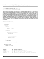
4.2
INDEXSETS (Mandatory) . . . . . . . . . . . . . . . . . . . . . . . . . . . . . .
44
4.3
LDSDESC (mandatory) . . . . . . . . . . . . . . . . . . . . . . . . . . . . . . . .
46
Examples
50
5.1
Examples for domain decomposition with vertical refinement . . . . . . . . . . . .
50
5.1.1
Example SIMINP file for domain decomposition with vertical refinement .
50
5.1.2
Example include files for vertical refinement . . . . . . . . . . . . . . . .
52
5.1.3
Example areas file for vertical refinement . . . . . . . . . . . . . . . . . .
53
5.1.4
Example call of the run procedures for vertical refinement . . . . . . . . .
53
5.1.5
Example call for vertical refinement using automatic partitioning . . . . . .
53
Examples for domain decomposition with horizontal refinement . . . . . . . . . .
54
5.2.1
Example process configuration file for horizontal refinement . . . . . . . .
54
5.2.2
Example call of the run-procedures for horizontal refinement . . . . . . . .
54
5.2.3
Example for horizontal refinement using automatic partitioning . . . . . .
55
5.3
Example partitioner configuration file . . . . . . . . . . . . . . . . . . . . . . . .
55
5.4
Example partitioning Input file . . . . . . . . . . . . . . . . . . . . . . . . . . . .
57
5.5
Example LDS description . . . . . . . . . . . . . . . . . . . . . . . . . . . . . . .
61
5.2
A Glossary of terms
I
Version 2.20, June 2011
1
User’s Guide for Parallel WAQUA/TRIWAQ and for Domain Decomposition
Chapter 1
Introduction
1.1
Parallel computing
In this section we give a concise introduction to parallel computing, and define a bit of terminology
used in this area.
Parallel computing is to use multiple computers or processors simultaneously for a single computing task in order to reduce the turn-around time.
The use of parallel computing requires that the following aspects be considered:
• The type of computing hardware to be used,
• The way of programming of the parallel computing hardware,
• The distribution of a computing task into more or less independent subtasks,
• (In some parallel programming methodologies) the distribution of the problem data over the
different subtasks,
• (In some parallel programming methodologies) the determination of the communication requirements between the different subtasks,
• (In some parallel programming methodologies) the determination of the synchronization requirements between the different subtasks.
In this section we briefly introduce current parallel computing hardware and programming methodologies, and give an overview of the parallelization approach that is adopted for parallel WAQUA/
TRIWAQ.
The most popular parallel computers are nowadays clusters of fast off-the-shelf microprocessors,
with local cache and main memory modules, which are connected via an interconnection network.
2
Chapter 1. Introduction
Two important sub-classes are distinguished: networks of workstations (NOW) and symmetric multiprocessors (SMP). Networks of workstations are typically formed by users, by using different
computers together as a single computing resource, whereas symmetric multiprocessors are typically designed and built by hardware vendors such as IBM, SGI, HP and SUN.
Networks of workstations typically employ standard technology. The most important example of
this class of parallel computers is the cluster of Linux PC’s connected via (fast) Ethernet networks,
which are often called Beowulf systems.
Symmetric multiprocessors on the other hand typically use components that are specifically designed for parallel computing. This concerns for instance the interconnection network, with lowlatency/high throughput routing chips and optimized topologies. Further many current SMP-type
systems are extended with mechanisms for cache coherency and for automatic migration of memory
pages, such that the system can be used as if it contains a single shared memory module. However,
if the memory is physically distributed then treating it as shared memory may introduce substantial
performance degradation.
The most popular parallel computing methodologies are nowadays data parallel programming,
shared memory programming and message passing. Data parallel programming uses special programming languages (High Performance Fortran), shared memory-programming (e.g. with Fortran
with OpenMP extensions) assumes a single ’name space’ for variables accessible to all computing
processes, and uses synchronization mechanisms, and message passing (PVM, MPI) uses separate
’name spaces’ per computing process, inaccessible to other computing processes, and communication mechanisms.
In Parallel WAQUA/TRIWAQ the message-passing paradigm is adopted. Separate WAQUA/ TRIWAQ computing processes are introduced that all take care of a specific section of the global computational domain. The computing processes communicate with each other for exchange of intermediate results at subdomain interfaces and for coordination of iterative solution procedures. Initial
data for the subdomain problems are determined automatically from the initial data for the global
domain, and output data for the subdomain problems are collected automatically into a global output file.
Parallel WAQUA/TRIWAQ can be used on NOW-type parallel computers as well as on SMP’s. In
all cases parallel computing is beneficial for larger simulations only, such that the communication
times are relatively small compared to the computing times. On NOW’s communication times are
usually larger than on SMP’s, such that less processors can be used effectively for a comparable
sized simulation. On a large scale SGI Origin2000 system called "Unite" successful simulations
have been carried out for the Rymamo-model with TRIWAQ on 64 processors. On Linux clusters
the maximum number of processors that have been used efficiently is currently about 20.
Version 2.20, June 2011
3
User’s Guide for Parallel WAQUA/TRIWAQ and for Domain Decomposition
1.2
Parallel computing for WAQUA/TRIWAQ
Parallel WAQUA/TRIWAQ is the parallel version of WAQUA/TRIWAQ in SIMONA. It consists of
the following parts:
• A partitioner COPPRE, that is to be called after the preprocessor WAQPRE but before the
parallel version of WAQUA/TRIWAQ. This preprocessor has its own (configuration) input
file, in which the user can specify a.o. the number of processors and the partitioning method
to be used, and details regarding the architecture of the parallel platform. COPPRE splits the
global SDS file into smaller SDS-files, one for each parallel process.
• A parallel version of WAQUA/TRIWAQ, that consist of an executive process COEXEC and
as many WAQUA/TRIWAQ processes as requested by the user. Each WAQUA/TRIWAQ
process performs computations using its own SDS-file. The WAQUA/TRIWAQ program
is capable to exchange intermediate results with other WAQUA/TRIWAQ processes and to
communicate with the master process COEXEC. The communication routines are part of a
communication library, COCLIB that has been developed for this application, but which is
designed in an application-independent way.
• A collector COPPOS, that is to be called after the parallel execution of WAQUA/TRIWAQ.
It collects the data from the SDS-files of all WAQUA/TRIWAQ processes into one SDS-file,
which can then be used for post processing in the ordinary, sequential way.
The partitioning that is done by COPPRE is based on the specification of the grid in the SDS-file.
Only structured grids are allowed (rectilinear, curvilinear or spherical, using the MESH_LGRID
table). COPPRE can take the target parallel architecture into account in the partitioning: the faster
processors get a larger part of the MESH than the slower ones.
The modifications to the WAQUA/TRIWAQ program are such that the functionality of the program
remains the same as the original non-parallel version if it is run on a single processor.
1.3
Domain decomposition with horizontal and vertical refinement
Many of the models on which WAQUA and TRIWAQ is used, cover regions with varying characteristics. For example, the Zeedelta model contains a part of the open sea, a harbour region and
many rivers and canals. The regions near the open sea contain salt water and the water movement
is determined mostly by wind and tide. The water in the river regions, on the other hand, is not salt
and the movement is hardly affected by wind and tide.
Some of these regions need a fine grid and many layers in order to get sufficiently accurate results,
whereas other regions could do with a much coarser grid and fewer layers. For instance a fine
(horizontal or vertical) grid is needed in regions where the flow field changes a lot over relatively
4
Chapter 1. Introduction
small distances, e.g. harbour areas with relatively small geometrical features, near sluices, and in
regions with strong density effects or stratification, whereas a coarse grid can be used at open sea.
So, ideally, one would like to be able to choose the fineness of the grid and the number of layers in
each region independently.
Another motivation for using domain decomposition is that it may simplify the working with nested
models, where the boundary conditions of a smaller scale model are generated using a large-scale
model. Using domain decomposition the values at the boundaries of the detailed model may be
interpolated more accurately, and the restriction on the flow velocity to be perpendicular to the
boundaries is eliminated. Further a two-way coupling is achieved such that the results of the finer
scale model are incorporated in the large-scale model, which improves the overall results of the
simulation.
These goals can be achieved with the domain decomposition functionality of WAQUA and TRIWAQ. In the context of domain decomposition with horizontal grid refinement, the total area of
interest is divided into different regions that are modelled separately in multiple simulation input
files. The different regions are called (global) domains and for each region a grid is defined. The
regions may also be defined by excluding certain areas of existing large-scale models, i.e. re-using
existing model input files. The different global domains are then simulated simultaneously, and
thereby use model results of each other on their mutual interfaces.
In the context of domain decomposition with vertical refinement (only possible for TRIWAQ), there
are two approaches possible:
1. Only a single horizontal grid needs to be defined, and therefore only one global domain/model
input file is used. This global domain is then decomposed into different parts that are called
subdomains. The number of layers in the subdomains can then be chosen to match the characteristics of the corresponding, physical region.
2. Like horizontal refinement, multiple global domains with the same horizontal grid are defined.
The number of layers/layer distribution differs between these global domains (this is in fact a
special case of horizontal refinement combined with vertical refinement)
Note: the user is advised to follow the first approach if only one model is used in the computation.
The computations are slightly more efficient and the results will be collected into a single SDS-file
instead of a separate file for each domain.
As already mentioned, it is also possible to combine horizontal refinement with vertical refinement.
In that case multiple global domains must be specified like using only horizontal refinement. These
global domains however can be dived in a number of sub-domains that have a different number of
layers/layer distribution. (like approach 1. of vertical refinement). Simultaneously it is also allowed
to have a different vertical refinement between the global domains.
In the current implementation of domain decomposition for WAQUA/TRIWAQ some restrictions
are imposed on connection of the grids of different domains or subdomains at their mutual interVersion 2.20, June 2011
5
User’s Guide for Parallel WAQUA/TRIWAQ and for Domain Decomposition
faces. In the horizontal direction, the interface is located at cell-faces, which must coincide for the
different domains involved. A domain will be called coarse if it has fewer cell-faces on the interface
than a neighbouring domain and fine if it has more. In the context of vertical refinement, a subdomain is called coarse if it has fewer layers than another subdomain (and fine if it has more).
Between two neighbouring subdomains it is not allowed that one of them is finer horizontally and
the other is finer vertically. And similarly a domain/subdomain may not be coarser than a neighbouring domain on one part of their interface and finer on another.
1.4
Domain decomposition with vertical refinement with TRIWAQ
In the previous section it was explained that horizontal grid refinement requires multiple simulation
input-files/domains, whereas vertical refinement can also be realized using a single domain. The
case where vertical refinement is realized using multiple input-files/domains is considered to be a
special case of the combination of horizontal and vertical refinement and is not discussed in this
section. The use of a single input-file/domain allows for an implementation that makes it relatively
simple for users to work with domain decomposition with vertical grid refinement.
In this section we give a brief introduction to the way in which domain decomposition with vertical
refinement is realized for TRIWAQ.
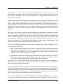
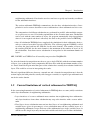
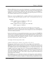
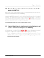
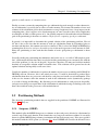
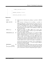
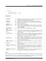
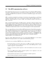
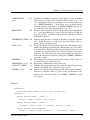
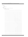
A schematic representation of the system is given in Figure 1.1. More information can be found in
the Design Document (Technical Report TR01-02, VORtech Computing) and in the system documentation.
Doing a domain decomposition run with TRIWAQ with vertical refinement involves the following
steps:
• The user creates a normal (siminp-) input file for WAQPRE for the full domain. With this
input file, the user can do initial experiments to validate the model and to determine whether
there are parts of the model that should be computed with more or with fewer layers.
• If the user decides to use a vertically refined grid, he or she will make a few small modifications to the input file: the value of KMAX will be replaced by the reserved string "%KMAX%"
and all information that varies between subdomains (like the layer thicknesses) are specified
by including files that have the number of layers or subdomain number in their names. Also
weir-definitions must be treated in this way because they are allowed in TRIWAQ in runs with
a single layer only. In the siminp file, the subdomain number in the include-file name is not
given explicitly, but by the reserved strings "%KMAX%" or "%DOM%". So, for example,
layer thicknesses may be specified as:
6
Chapter 1. Introduction
VERTICAL
INCLUDE FILE="layer_def.%DOM%"
• Next, the user specifies a splitting of the domain into subdomains, by writing a so-called
areas-file, which defines the subdomains in terms of boxes in the full domain. Furthermore,
the user writes for each subdomain the include-files that have to be included in the siminp
file. In the example above, the user will create files layer_def.1, layer_def.2, etc., one for each
subdomain.
• The remaining steps of running domain decomposition are done automatically by the runprocedures. First, for each subdomain,
– The string %KMAX% in the model input file is replaced by the number of layers for the
subdomain and the string %DOM% is replaced by the subdomain number.
– WAQPRE is called to create an SDS-file with the specified layer distribution for the
entire domain.
– COPPRE is called to extract the subdomain data from this SDS-file and create an SDSfile for the subdomain (which has the same name as the SDS-file for the entire domain,
but with a three-digit subdomain number appended to it).
These tasks are performed by run-procedure WAQPRE.PL.
Note: WAQPRE and COPPRE are run separately for each subdomain when the construct
%DOM% is used. When %DOM% is not used, they are run for each distinct value of kmax.
In that case, subdomains with the same number of layers will be generated together in a single
pass and the performance will be improved.
Now that SDS-files have been created for each subdomain, the run-procedure WAQPRO.PL first
starts the MPI system (which provides the mechanisms for inter process communication) and then
starts the COEXEC program and the TRIWAQ processes for each of the subdomains. The COEXEC
program keeps running until the last subdomain-TRIWAQ has ended. Its main task is to perform
checks for domain decomposition; its task used to be larger when we were using PVM instead of
MPI.
The message output of the TRIWAQ processes is first written to separate output-files waqprom.<runid>-xxx. After completion of the run all output is gathered into a single message-file. A
similar mechanism is used for bulk data file-I/O: the subdomain TRIWAQs write output to their
own SDS-file, and these SDS-files are collected into a single file for the global domain after completion of the run. The bulk print files are however not joined together; these are provided separately
for each subdomain in waqpro-r.<runid>-xxx.
• The TRIWAQ processes per subdomain perform the usual computations on their subdomains.
However, the subdomains contain a new type of boundary condition: the subdomain interface.
On these boundaries, the boundary conditions are obtained through communication with the
Version 2.20, June 2011
7
User’s Guide for Parallel WAQUA/TRIWAQ and for Domain Decomposition
incl-1
input
areas
incl-N
waqpre.pl
WAQPRE
....
lds
WAQPRE
cfg
SDS-dom
COPPRE
SDS-dom-1
SDS-dom
....
COPPRE
....
SDS-dom-N
waqpro.pl
prc
COEXEC
TRIWAQ
....
TRIWAQ
TRIWAQ
COCLIB
SDS-dom-1
....
SDS-dom-N
COPPOS
SDS-dom
msg
Figure 1.1: Schematic overview of the TRIWAQ system with domain decomposition with vertical grid refinement
8
Chapter 1. Introduction
neighbouring subdomain. Note that the user does not have to specify any boundary conditions
for the subdomain interfaces.
The various subdomain TRIWAQs communicate data for these subdomain interfaces. Interpolation is used to convert data from a coarse subdomain to a finer subdomain and vice versa.
The computations for different subdomains are performed in parallel, when multiple computers or processors are used. For further optimisation of the execution time more subdomains
can be used with the same number of layers; the program automatically skips interpolation
where it is not required and then is effectively the same as the parallel version of TRIWAQ.
• Once all subdomain TRIWAQs have completed the simulation for their subdomain, their results are scattered over their respective SDS-files. The collector program COPPOS is called
to collect the data back into the SDS-file for the entire domain. The number of layers in
the resulting SDS-file for the entire domain is the maximum of the number of layers of all
the subdomains. Data from coarser subdomains is interpolated to this maximum number of
layers.
MPI, COEXEC and COPPOS are all started by run-procedure WAQPRO.PL.
So, after the domain decomposition run, the user gets a single SDS-file with the maximum number
of layers, just as though the entire computation had been done with this maximum number of layers. But it should be kept in mind that parts of the solution have actually been obtained with fewer
layers. This could be an issue in interpreting the results.
The only significant difference between a normal run and a domain decomposition run is that the
written output (the bulk print-file, usually called waqpro-r.<runid>) is organised per subdomain and
not for the entire domain.
1.5
Current limitations of vertical refinement in TRIWAQ
In the current implementation of vertical refinement in TRIWAQ there are some (mild) restrictions
on the layer distributions of neighbouring subdomains:
• Layer interfaces of a coarse subdomain must continue into neighbouring finer subdomains;
only layer interfaces from a finer subdomain may stop at the interface with a coarser subdomain.
• Fixed layers in one subdomain must run into fixed layers of a neighbouring subdomain and
variable layers (given in percentages) of one subdomain must run into variable layers of a
neighbouring subdomain, except when one of the subdomains has a single (variable) layer, in
which case this single layer may run into both variable and fixed layers in other subdomains.
Version 2.20, June 2011
9
User’s Guide for Parallel WAQUA/TRIWAQ and for Domain Decomposition
• The number of layers in the finer subdomain that meet a particular layer in the coarser subdomain (i.e. the degree of refinement) must be at most four. If this number is higher, the
functionality will still work, but numerical artefacts may become serious. So, if one wants
to go from 1 layer in one subdomain to 16 layers in another, there should be at least one
subdomain (with four layers) in between.
• If a subdomain with only one layer connects to a subdomain with both fixed and variable
thickness layers, the velocity and transport checkpoints in the subdomain with one layer must
also be water level checkpoints. This is necessary for the interpolations done by the collector
program COPPOS.
• The use of weirs exactly on subdomain interfaces is not advised, especially because in future
versions the interfaces may be assigned to the subdomain with the highest number of layers
of the two neighbouring subdomains, instead to the left/lower subdomain.
• The subdomain with the highest number must also have the maximum number of layers.
Restrictions on the decomposition of a domain into subdomains are given in Section 2.2.
1.6
Domain decomposition with horizontal refinement with WAQUA
and TRIWAQ
In this section we give a brief introduction to the way in which domain decomposition with horizontal refinement is realized for WAQUA and TRIWAQ.
Domain decomposition with horizontal grid refinement in WAQUA/TRIWAQ starts from the definition of multiple domains, with computational grids that agree with each other on mutual interfaces.
These interfaces consist of the sides of computational cells, that is, the velocity points. The so-called
depth grid locations of a coarse domain must coincide with depth points of a fine domain.
For each domain separately a simulation input-file is created. Each domain may be split into multiple subdomains (for parallel computation or vertical refinement), and also one part of each domain
(not necessarily coherent) may be taken out of the computation. This is useful for instance when
part of an overall model schematisation is refined in a detailed model. The simulation input-file of
the overall model can then be reused without modification; the parts that are filled in by the detailed
model are assigned to the "inactive part of the domain" and will not be computed using the overall
model.
The pre-processing stage of the computation (execution of pre-processor WAQPRE) is carried out
separately per domain. The resulting SIMONA data storage files are split into the required number
of parts for the different subdomains. Finally the simulation of all subdomains is carried out simultaneously using multiple WAQUA/TRIWAQ computing processes that exchange of information at
10
Chapter 1. Introduction
subdomain boundaries.
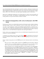
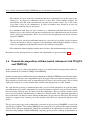
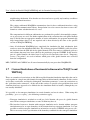
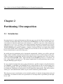
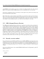
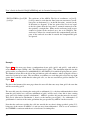
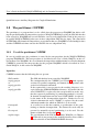
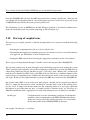
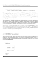
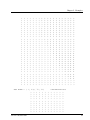
A schematic representation of this system is given in Figure 1.2. More information can be found in
the Design Document (Technical Report TR01-06, VORtech Computing) and in the system documentation.
Doing a domain decomposition run with WAQUA/TRIWAQ with horizontal refinement involves the
following steps:
• The user creates a number of normal (siminp-) input files for WAQPRE for the global domains
that are distinguished. With these input files, the user can do initial experiments to validate
the models and to determine whether there are parts of the models that should be computed
with a coarser or finer grid. In the following we will consider as an example of this the on-line
coupling of a "Kuststrook" model with the "Rymamo" model, which were initially defined for
stand-alone computation. However, it is not necessary that the separate simulation input-files
produce meaningful results by themselves, as we will indicate later on.
• Next, the user determines precisely how the grids of all global domains should be joined together. Different grids can be connected at interior points or at open boundaries. In all cases
the interface of a domain goes through velocity points, just like discharge cross-sections.
In case of the coupling of Rymamo and Kuststrook, we want to use Rymamo in its entirety,
and want to exclude from the Kuststrook model the region that is incorporated in the Rymamo
model. The Rymamo model is then connected to the Kuststrook on its open sea boundaries.
For the Kuststrook model we determine precisely which grid cells must be marked "inactive",
which grid cells are covered by the Rymamo model.
• For all global domains a splitting into subdomains is defined, by writing a so-called areas-file.
An areas file defines the subdomains in terms of boxes or enclosures in the full domain.
For the Rymamo model a single area is sufficient that assigns all grid cells to subdomain 1:
AREA 1
SUBDOMAIN 1
MNMNBOX 1, 1, 10000, 10000
Also multiple subdomains may be defined in order to use parallel computation for the Rymamo model. For the Kuststrook model at least two areas are needed: for the active and the
inactive part of the domain (subdomain number "-1"). The construction of appropriate areas
should not be too hard, as long as the user knows precisely which grid cells must be included
in the computation. Also IPW may be used to generate the appropriate areas-files. More information on the creation of areas-files is given in Paragraph 2.6.
Version 2.20, June 2011
11
User’s Guide for Parallel WAQUA/TRIWAQ and for Domain Decomposition
inp-d1
area-d1
inp-dN
area-dN
waqpre.pl
waqpre.pl
WAQPRE
WAQPRE
....
SDS-d1
SDS-dN
COPPRE
COPPRE
SDS-d1-1
....
SDS-d1-n1
....
SDS-dN-1
SDS-dN-nN
cfg
waqpro.pl
COEXEC
WAQPRO
....
WAQPRO
WAQPRO
....
COCLIB
SDS-d1-1
....
....
SDS-d1-n1
SDS-dN-nN
....
COPPOS
COPPOS
SDS-d1
SDS-dN
msg
Figure 1.2: Schematic overview of the WAQUA/TRIWAQ system with domain decomposition
with horizontal grid refinement
• Next the pre-processing stage is carried out for each domain separately, by running the runprocedure WAQPRE.PL for a simulation input file plus the corresponding areas file. This
will
– call WAQPRE to create an SDS-file for the entire domain.
– call COPPRE to extract the subdomain data from this SDS-file for all active subdomains,
and create SDS-files for the subdomains (which have the same name as the SDS-file for
the global domain, extended by a three-digit subdomain number). Further COPPRE extends the arrays in the SDS-file with a few additional grid rows and columns to facilitate
for the communication between different subdomains later on.
12
Chapter 1. Introduction
• When the SDS-files have been created for all subdomains, it is advisable to check their consistency before starting the actual simulation. This checks whether the different grids match
to each other on their interfaces, whether the same process-models are used (WAQUA vs.
TRIWAQ, yes/no transport simulation), and whether some important parameters are the same
in the different domains (time-step, layer distribution, ...).
Either way a "process configuration file" is required, which lists the domains that must be
combined in a single simulation together with their "runid’s" and experiment names used, e.g.
DOMAINS
DOM 1, NAME=’Rymamo’, RUNID=’rym’, EXP=’rym’,
EXEC=’waqpro.exe’, BUFS=20
DOM 2, NAME=’Kuststrook’, RUNID=’kust’, EXP=’k90’
EXEC=’waqpro.exe’, BUFS=10
The executable-name used in this example shows how the buffer-size for the program
WAQPRO.EXE is specified. This size is the same for all subdomains of a single global domain, but may vary between global domains. In the example the size 20 is used for Rymamo
and 10 for the Kuststrook model.
Besides the runid’s that are used per global domain in the pre-processing stage (WAQPRE.PL)
and that are used to identify the SDS-files for the different global domains, a separate runid is
used to identify a simulation with horizontal refinement. This runid is used only for the name
of the message-file of the entire simulation. It could be "rym_kust", which would result in a
message-file with the name "waqpro-m.rym_kust".
An example call of the run-procedure is then
waqpro.pl -runid rym_kust -config proc_cfg.rym_kust -check_only yes
• Then the actual simulation may be started. This is done using the same run-procedure
WAQPRO.PL, but now with the option check_only omitted. The run-procedure first starts the
MPI system (which provides the mechanisms for inter process communication) and then starts
the COEXEC program and the WAQUA/TRIWAQ processes for each of the subdomains. The
COEXEC program keeps running until the last subdomain-WAQUA/TRIWAQ process has
ended. The subdomain WAQPROs produce separate output-files: they all write to their own
message-file, bulk print-file and SDS-file during the run. After completion of the run the
message files and SDS-files will be collected into a single message-file and an SDS-file per
global domain of the simulation.
• The WAQPRO processes per subdomain perform the usual computations on their subdomains.
However, the subdomains contain a new type of boundary condition: the subdomain interface.
On these boundaries, the boundary conditions are obtained through communication with the
Version 2.20, June 2011
13
User’s Guide for Parallel WAQUA/TRIWAQ and for Domain Decomposition
neighbouring subdomain. Note that the user does not have to specify any boundary conditions
for the subdomain interfaces.
The various subdomain WAQPROs communicate data for these subdomain interfaces using
the COCLIB communications library. Interpolation is used to convert data from a coarse subdomain to a finer subdomain and vice versa.
The computations for different subdomains are performed in parallel, when multiple computers or processors are used. For further optimisation of the execution time each global domain
may be divided into an appropriate number of active subdomains; the program automatically
skips interpolation where it is not required and is then effectively the same as the parallel
version of WAQUA/TRIWAQ.
• Once all subdomain WAQPROs have completed the simulation for their subdomain, their
results are stored in subdomain SDS-files. The collector program COPPOS is called to collect
the data back into the SDS-file for the global domain. This also removes additional grid rows
and columns that may have been added by the partitioner program COPPRE. In the inactive
part of a global domain, the initial state is copied to all consecutive time levels. Temporary
screens ("dry points") are used to indicate which parts of the global domain were excluded
from the computation.
MPI, COEXEC and COPPOS are all started automatically by run-procedure WAQPRO.PL.
1.7
Current limitations of horizontal refinement in WAQUA and
TRIWAQ
There are a number of restrictions on the different global domains/simulation input files that can be
used together in a single run with domain decomposition with horizontal refinement. In this section
we list these restrictions, and thereby distinguish "simulation parameters" versus the restrictions on
the "grids that can be connected". At the end of this section, we provide a few guidelines that avoid
situations that have appeared to be difficult for the simulation model to handle, although they are
not actually forbidden.
It is possible to do transport-simulations in certain domains and not in others. When using this
possibility (’process coupling’), the following restrictions apply:
• Transport simulation is switched on or off per global domain: the parts of a global domain
must all have transport simulation, or none of them may have it.
• The interface between a domain with transport simulation and a domain without transport
simulation must be an open boundary of the domain that has transport simulation. It is not
possible to end the transport simulation at an interface created by COPPRE, using an area file,
This is necessary for the specification of the boundary conditions fro the transport simulation.
14
Chapter 1. Introduction
• All domains which have transport simulation must have the same transported species, specified in the input in the same order.
NB: this restriction is not sufficiently checked: only the number of transported species is
checked. Unexpected results may be obtained when the transported substances are given in
different orders in different domains!
It is also possible to use turbulence transport calculation in some domains, and not in others. Only
one of the restrictions above applies:
• Turbulence transport is switched on or off per global domain: the parts of a global domain
must all have it, or none of them may have it.
The other restrictions do not apply because boundary conditions need not be supplied for the turbulence model.
In the current implementation of horizontal refinement for WAQUA and TRIWAQ following restrictions are imposed on the different simulation input files:
• All domains must use WAQUA, or otherwise all domains must describe a TRIWAQ simulation; combination of WAQUA and TRIWAQ within a single run is not supported.
• Lagrangian time integration and the user-transport routine are not available when using domain decomposition.
• When using spatially varying wind and pressure, the name of the wind SDS-files must be
different for all global domains. Note that it is allowed to use spatially varying wind and
pressure in some of the domains only, although care must be taken in this case to provide
wind fields that fit to each other at domain interfaces.
• Different roughness formulations may be used in different global domains; however,
k-Nikuradse roughness computation must be used in all domains or in none of them.
• Time-step parameters must be the same in all global domains. Particularly it is verified that
the timeframe of the simulation is consistent, that the times at which bottom-friction processes
are re-computed are the same, and that status-information is printed at the same times.
• Also iteration parameters must be the same in all global domains: flags CHECK_CONT,
ITERMOM, ITERCONT and the different iteration accuracies.
• When one of the domains (at horizontal refinement) uses CHECK_WL=’yes’, all other domains must use this as well.
The following restrictions are imposed on the grids that are to be connected in a single simulation:
• For each pair of domains one of them must be finer than or equally fine as the other in their
entire mutual interface, or they must match without refinement everywhere. The situation
where a domain is both finer than a neighbour in one part and coarser in another part of their
mutual interface is not supported.
Version 2.20, June 2011
15
User’s Guide for Parallel WAQUA/TRIWAQ and for Domain Decomposition
• The grids to be connected must have the same orientation; x/ξ- resp. y/η grid lines of one
domain can be connected to x/ξ- resp. y/η grid lines of another domain only, and the directions
in which x/ξ- and y/η-coordinates increase must be the same in both domains.
• The interfaces of different domains consist of "curves" in the horizontal plane, which pass
through corners of grid cells: depth points and velocity points of the WAQUA grid. The depth
points on the interface of a coarser domain must coincide with depth-points on the interface
of a finer domain.
• The fine domain’s interface may be slightly wider or narrower than the coarse grid’s interface.
If the interface of the fine grid is slightly wider, however, there will be fine grid cell-faces
(u/v-points), which do not connect to coarse grid cell-faces (u/v-points). These will be closed
off using screens ("schotjes"). A warning will be issued in such cases.
• Different interfaces must stay away from each other by at least 3.5 grid spaces w.r.t. the
coarsest domain involved, except for interfaces that start/end in a single point.
• Different interfaces (e.g. open boundaries) of the same global domain may not be connected
to each other. Grid lines may not be connected in such a way that there is no global start and
end-point.
• The use of refinement factors > 4 is not advisable, because this may lead to less accurate
simulation results. Also strongly curved grid lines near interfaces of different domains are
dissuaded for this reason.
Finally there are some restrictions on the specification of the inactive part of a domain:
• Openings, line-barriers and cross-sections may not lie partly in an active subdomain of a
domain and partly in the inactive area. Subdivision of these constructs over different active
subdomains is supported; just as in parallel WAQUA/TRIWAQ virtually any partitioning can
be accommodated.
• None of the checkpoints or cross-sections that are used in the conditions of the dynamic
barrier steering mechanism may lie in the inactive area of a domain. Note further that the
dynamic barrier steering mechanism cannot refer to information of other global domains, by
virtue of the separate pre-processing for different global domains.
Finally, the following rules can be used to avoid situations that can prove to be problematic for the
software, although they are not formally prohibited:
• If possible, choose your interfaces (i.e. locations where different grids are coupled) at locations with as few model details as possible. In particular, do not define interfaces at places
with strong variation in bottom topography, near weirs or barriers etc.
• Make interfaces as straight as possible, i.e. do not use corners in the interfaces if they can be
avoided. In any case, use constant refinement factors around corners in the interfaces.
16
Chapter 1. Introduction
1.8
Domain decomposition with horizontal and vertical refinement with TRIWAQ
In this section we give a brief introduction to the way in which domain decomposition with horizontal and vertical refinement is realized for TRIWAQ.
A number of global domains must be created, similar to domain decomposition with horizontal
refinement. The different global domains can have a different number of layers. It is possible to
create one or more of the global domains as explained in Section 1.4. The global domain contains
subdomains with different numbers of layers in that case. The area file can specify the inactive parts
(subdomain -1) when the domain is not coupled at its openings.
The different global domains can also have a different number of layers.
1.9
Current limitations to simultaneously using horizontal and
vertical refinement in WAQUA and TRIWAQ
All the restrictions as mentioned in Section 1.5 and 1.7 for vertical and respectively horizontal
refinement do also apply to the combination of both. There is only one extra restriction:
• In every coupling of two (sub)domains, it must be possible to determine which of the two
neighbours is finer. Therefore, if one has a finer horizontal grid, it may not have coarser layer
distribution. Of course, the two neighbours may also have an equally fine grid, both in the
horizontal and vertical directions.
Version 2.20, June 2011
17
User’s Guide for Parallel WAQUA/TRIWAQ and for Domain Decomposition
Chapter 2
Partitioning / Decomposition
2.1
Introduction
Decomposition of a single grid/domain into different parts is needed in different situations. In case
of domain decomposition with vertical refinement with TRIWAQ the user must decide which vertical resolution is wanted in which areas of the domain, i.e. which decomposition of the domain into
subdomains is to be used. Secondly, when using horizontal refinement or horizontal and vertical
refinement is used, a part of the grid may be excluded from the computation. Finally, when running
WAQUA/TRIWAQ on a parallel computer, a (further) decision will have to be made about which
part of each domain will be computed on which processor. In this case the user will have to specify
how the domain must be partitioned into parts.
In parallel runs the partitioning can be determined automatically. Mostly, users will be perfectly
happy with the standard setting, but for particular experiments it can be useful to improve the partitioning. An improved partitioning can have a large impact on the computing speed, and, on systems
such as the SGI Origin2000 "Unite" where idle time of the WAQPRO processes is accounted, can
have a large impact on the total cost. The manual optimization of grid partitionings may be done
using the Matlab program Visipart.
In case a domain decomposition run is to be performed on a parallel computer, the global domains
(for DDHOR) or subdomains (for DDVERT) may be divided further by the user into multiple parts
for parallel computing. For this the auxiliary program Visipart may be used. A new possibility is
to partition the subdomains for horizontal or vertical refinement automatically. This can be done by
entering for each subdomain the number of parts and the automatic partition method.
This chapter presents considerations on the desirable qualities of domain decompositions and grid
partitionings, and further describes the specification of a decomposition or partitioning in the input
(areas-) file.
18
Chapter 2. Partitioning / Decomposition
2.2
Creating a suitable splitting of the domain
The following issues should be kept in mind when defining a decomposition of an area of interest
into different domains for horizontal refinement, and defining a decomposition of the mesh of a
global domain into subdomains for use with vertical grid refinement or parallel computation.
• The number of domains and subdomains should be kept as small as possible. In case of
vertical refinement this is because WAQPRE and COPPRE may be executed separately for
each subdomain, which may take quite some time especially if the full mesh is large. Also,
computational performance may degrade if the number of subdomains is very large.
• Subdomain interfaces must stay away from each other, from open boundaries and from barrier
points. So it is not allowed to create very small or narrow subdomains. Subdomain interfaces
may be perpendicular to an open boundary, though. This allows for cutting through horizontal
or vertical openings. Diagonal openings cannot be cut by subdomain interfaces because then
part of the boundary will actually be parallel to the subdomain interface.
• It is useful to create subdomains with a small full box (or rather: a high fill ratio), because a
small full box usually leads to better computational performance and less memory consumption. If a subdomain has a small full box, then the buffer size for the WAQPRO process that
will do its computations can be set small (see option -bufsize of the run procedure waqpro.pl).
• If more than one processor is available, then the subdomains will be distributed over the available processors in a way such that every processor is about equally loaded. (There are more
options for mapping subdomains onto processors, see paragraph 2.10.)
To get an impression of the load that will be produced by a subdomain, check the file copprer.<runid>, which gives the number of grid points in each subdomain. This number of grid
points, multiplied by the number of layers of the subdomain, gives a rough indication of the
computational load of the subdomain.
• In case more than one processor is used, it is also beneficial to choose subdomain numbers
such that neighbouring subdomains are mapped onto the same processor. This usually improves the speed of communication between these subdomains.
Additional restrictions on the decomposition of a domain for vertical refinement, especially regarding the layer distributions, are given in Section 1.5. Restrictions on the interfaces of domains for
horizontal refinement are given in Section 1.7.
2.3
The choice of the number of layers
The first tests with domain decomposition with vertical refinement have indicated the following
issues in selecting the number of layers per subdomain:
Version 2.20, June 2011
19
User’s Guide for Parallel WAQUA/TRIWAQ and for Domain Decomposition
• Keeping the number of layers small will save a lot of computing time, but it should be done
with care. Verify the solution wherever possible to make sure that the number of layers has
not been chosen too small.
• Changing the number of layers in a subdomain could necessitate a change in other parameters
for that subdomain. In particular the diffusion parameters should be set to match the number
of layers.
• The choice for a single layer in one of the subdomains can have a strong impact on the numerical results, because not all three-dimensional processes can be adequately represented in
a single layer.
This section will be extended when more experience has been gained with vertical grid refinement.
2.4
Creating a suitable partitioning for parallel computing
In determining a partitioning of the computational domain for parallel computing, the aim is to
choose the sizes of the subdomains such that every processor will need about the same amount of
time to complete the computations for the subdomains that have been allocated to it. If this aim
is not met, then some of the processors will have more work to do than others, which leads to inefficient use of the parallel system. Note that especially the largest subdomain is of interest here,
because all other subdomains have to wait for this one; it is much less important to increase the size
of a subdomain that is smaller than average. When each processor gets the same amount of work to
do, it is said that the partitioning provides a good load balance.
At the same time, the partitioning must also be done in such a way that the border between any two
subdomains is as small as possible. This is important, because the subdomains are connected on
their borders and consequently, the amount of communication between processors is roughly indicated by the size of the borders of the subdomains that are allocated to them. As communication
is a form of overhead that reduces the efficiency of a parallel computation, it should be minimized
and hence the borders between subdomains should be as small as possible. If a partitioning results
in small borders, it is said that it provides a small communication volume.
Thirdly, it is sometimes advantageous to minimize not the size of the borders, but the number of
subdomains that are connected to a specific subdomain. To understand this, consider a subdomain
that is connected to four other subdomains. Then each time a communication is needed, the processor that handles the subdomain, will have to communicate with four other processors, and thus
has to send four messages. If the subdomain were instead connected to two other subdomains, the
processor would have to send only two messages. Now, sending a message always involves some
startup overhead (usually called latency) and therefore it is sometimes better to send one larger
message than to send two shorter ones. Thus, it can be advantageous to reduce the number of neighboring subdomains. A partitioning that minimizes the number of neighboring subdomains is said to
20
Chapter 2. Partitioning / Decomposition
provide a small number of communications.
Finally, on some systems the computing time per subdomain depends strongly on other characteristics of subdomains, especially due to effects of cache memory. For instance the number of rows and
columns of the subdomain grid or their maximum or average length may have a large impact on the
computing time. Also it appears to be disadvantageous on some systems to have array lengths that
are multiples of 1024 (or other powers of 2). On parallel computers with such behavior an additional
goal of the partitioning is therefore to achieve a high effective computing speed per subdomain.
In general, it is impossible to determine the optimal solution of the partitioning problem. First of
all, this is due to the fact that the amount of work per subdomain cannot be determined prior to
run-time and therefore, this amount can only be estimated. This is solved for WAQUA/TRIWAQ by
assuming that all interior and open boundary points in the mesh represent a fixed amount of work.
Hence the partitioning is done such that the number of active grid points per subdomain is about
equal.
Secondly, finding the partitioning that minimizes the border size is a so-called ’NP-complete problem’, which means that the time that is needed to find the partitioning grows extremely fast with the
size of the problem (i.e. the size of the grid). In practice, therefore, one must use heuristic methods
that find an acceptable solution within reasonable time. This solution will in general not be the
optimal solution, but hopefully it will come close.
Usually, the number of subdomains is equal to the number of processors on which parallel WAQUA/
TRIWAQ will run. However, this is not strictly necessary: it could be beneficial to produce more
subdomains than there are processors and then let each processor handle several subdomains. This
is the case for instance when the amount of work in the subdomains varies dynamically (perhaps
as a result of drying and flooding). By allocating several subdomains to each processor, hopefully,
each processor will get an equal share of the subdomains in which the drying or flooding occurs and
hence the workload on the processors will remain balanced.
2.5
Partitioning Methods
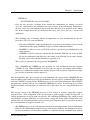
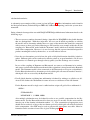
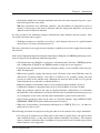
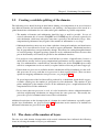
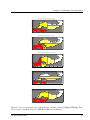
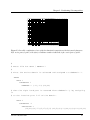
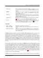
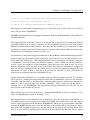
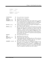
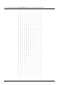
The (heuristic) partitioning methods that are supplied in the partitioner COPPRE are illustrated in
Figure 2.1. They are:
2.5.1
Stripwise (STRIP)
This method splits the MESH along rows or columns so that each part is effectively a (horizontal or
vertical) strip of the total domain. If the domain has very long rows and short columns, it is usually
better to split the MESH along columns (to minimize the border between parts). If the user specifies
this method with the ANY option (see Section 3.1), then COPPRE will consider the M and N-sizes
Version 2.20, June 2011
21
User’s Guide for Parallel WAQUA/TRIWAQ and for Domain Decomposition
of the MESH to decide whether a row wise or column wise splitting should be done. By using the
ROW or COL options with the STRIP method, the user can explicitly force one or the other.
Note that the subdomains will not necessarily be exactly equal in size (will not necessarily each
have the same number of grid points).
This method always assigns complete rows/columns to a part and never split a row into two parts.
Hence, a part may be larger if the total number of grid points in its rows is more than average. In the
same way, a part can be somewhat smaller. Usually, this effect is small, but it can become significant
if the number of rows/columns per part is very small or if rows/columns are very long.
2.5.2
ORB (Orthogonal Recursive Bisection)
The ORB method (Orthogonal Recursive Bisection, sometimes also called recursive coordinate bisection, RCB) first splits the domain into two strips using the stripwise method. Then each strip
is again split in two parts, where the border is chosen orthogonal to the one in the first splitting.
This procedure is repeated recursively until the required number of subdomains is reached. Strictly
speaking, this method can only create partitionings in which the number of parts is a power of two.
However, a slightly modified version is implemented in COPPRE that also allows for ORB partitioning into an arbitrary number of subdomains. If the number of parts is not a power of two, the
method will not split every part in the later stages of the recursion, but only a specific subset of the
parts. For example, if the number of parts is three, then first a splitting will be done into two parts
(of different sizes) and then only one of those parts will be split again into two parts.
2.5.3
Manually created or modified
By specifying the keyword PART_VALUES instead of PART_METHOD in the input file for the
partitioner (see Section 3.1) the partitioner can be directed to read the partitioning from file instead
of determining it by itself. This creates the possibility to use external partitioning packages or to
optimize an existing partitioning by hand. The latter is supported through the auxiliary program
Visipart.
One of the available formats is the standard SIMONA BOX format (See Programmer’s guide SIMONA, Section 3.2.3):
PART_VALUES
GLOBAL
LOCAL ...
22
Chapter 2. Partitioning / Decomposition
ORB COL partitioning of KTV model into 4 subdomains
30
25
4
n
20
2
15
3
10
1
5
10
20
30
40
50
60
70
60
70
m
ORB ROW partitioning of KTV model into 4 subdomains
30
25
4
3
n
20
1
15
10
1
2
5
10
20
30
40
50
m
STRIP COL partitioning of KTV model into 4 subdomains
30
25
4
n
20
3
15
2
1
10
5
10
20
30
40
50
60
70
m
STRIP ROW partitioning of KTV model into 4 subdomains
30
4
25
4
20
n
3
15
2
2
10
1
5
10
20
30
40
50
60
70
m
Manual partitioning of KTV model into 4 subdomains
30
25
4
n
20
2
3
15
10
1
5
10
20
30
40
50
60
70
m
Figure 2.1: The various partitioning methods that are available in Parallel WAQUA/TRIWAQ. From
top to bottom: Strip-Row, Strip-Col, ORB-Row, ORB-Col and Manual.
Version 2.20, June 2011
23
User’s Guide for Parallel WAQUA/TRIWAQ and for Domain Decomposition
Alternative formats are specified in Section 2.6 below. An example input file can be found in Section
5.4. A file in this format can also be produced by running the partitioner COPPRE once with any of
the automatic partitioning methods, and then edit the report print file, which contains a specification
of the partitioning that was created.
2.6
Format of the areas file
The decomposition of a domain into subdomains for domain decomposition, or the specification
of a user-defined partitioning for parallel computing is usually done by INCLUDing a so-called
areas file into one of the default partitioner configuration files (copcfg.gen.par, copcfg.gen.ddv
and copcfg.gen.ddh). Also the options -decomp and -partit of the run procedures waqpre.pl and
waqpro.pl take as argument such an areas file.
Note: If the last keyword block in the input file contains a sequential keyword, the SIMONA application independent preprocessor is not able to check the correctness of the block. This can result in
incorrect processing of the input file!
A decomposition of a domain into subdomains consists of an assignment of all (interior) grid cells
of the computational domain to subdomain numbers. Here grid cells may conveniently be identified
with waterlevel points in the WAQUA staggered grid. The format of the areas file is as follows (see
Section 5.1.3 for an example):
|AREAS
|
AREA [iseq]
|
SUBDOMAIN = [ival]
|
| <MNMNBOX ([ival1],[ival2])([ival3],[ival4])>
|
<
|
| ENCLOSURE <([ival1],[ival2])>
<
|PART_VALUES
|
|
LAYOUT = <[ival]>
|
| CONST_VALUES=<[ival]>
|
<
|
| VARIABLE_VALUES=<[ival]>
|
|
24
GLOBAL
LOCAL
< BOX: MNMN = ([ival1],[ival2])([ival3],[ival4])
Chapter 2. Partitioning / Decomposition
|
| CONST_VALUES=<[ival]>
|
<
|
| CORNER_VALUES=<[ival]>
|
<
|
| VARIABLE_VALUES=<[ival]>
Explanation:
AREAS
X1 Main keyword, indicating that splitting is specified in AREAS
form
PART_VALUES
X1 Main keyword, indicating that the splitting is specified in
PART_VALUES form. This keyword has the format of the standard SIMONA BOX mechanism. For more information about the
format, see the WAQUA user’s guide or the SIMONA programmer’s guide. The values of the field that is specified through the
BOX mechanism give the number of the subdomain to which each
of the points belongs.
AREA [iseq]
R
Keyword to specify one AREA. AREA’s may overlap, where
AREA’s with a higher sequence number [iseq] override AREA’s
with a lower sequence number.
SUBDOMAIN [ival]
M Specifies the number of the subdomain, ival, to which the AREA
belongs. Subdomains must be numbered consecutively, i.e. if the
highest subdomain number in an areas file is 7, then all subdomains 1...7 must be non-empty, at least one AREA must be assigned to them. In case of domain decomposition with vertical
refinement the subdomain with the highest number must also be
the subdomain with the maximum number of layers, and this subdomain number must be equal to the number of subdomains as
passed to the run-procedure (see below). In case of horizontal refinement the subdomain number "-1" is used to assign an AREA to
the inactive part of the domain.
X2 A box that belongs to the AREA. Boxes may overlap, where the
MNMNBOX
=
([ival1],
latest specified box has priority over boxes that have been specified
[ival2])([ival3],[ival4])
earlier. They may extend beyond the actual computational grid; the
parts of a box that lie outside the computational grid are ignored.
Version 2.20, June 2011
25
User’s Guide for Parallel WAQUA/TRIWAQ and for Domain Decomposition
ENCLOSURE=<([ival1],X2 The enclosure of the AREA. The list of coordinates =<([ival1],
[ival2])>
[ival2])> must be such that the lines between consecutive coordinate pairs are horizontal (i.e. in the M-direction), vertical (in the
N-direction) or diagonal. If the last point of the list is not equal
to the first point, then the last point is assumed connected to the
first point by a straight line. Points on the enclosure itself are not
counted as points in the enclosed area, just as in WAQUA. The
enclosure is allowed to extend outside the computational grid; the
parts of the enclosed area that lie outside the computational grid
are ignored.
Example
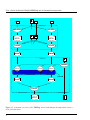
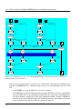
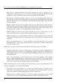
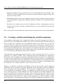
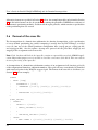
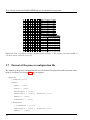
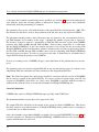
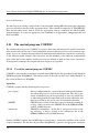
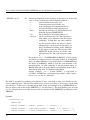
Figure 2.2 on the next page shows a configuration of two grids (grid 1 and grid 2), each with its
own simulation input (siminp-) file. The left-hand grid is grid 1. The simulation input file for this
grid specifies a rectangular area with MMAX=31 and NMAX=21 in which all grid points are active.
The numbers below and to the left of the grid indicate grid cell numbers, where each grid cell has a
water-level point in its centre. The curvilinear co-ordinates are such that grid cells in the top-right
corner have a smaller width than the other grid cells, see the true curvilinear grid for domain 1 in
Figure 2.3.
The box at the bottom of the next page shows the areas file that cuts away from grid 1 the area that
will be covered by grid 2.
The areas file starts by selecting the entire grid as subdomain 1 (i.e. the first subdomain that is taken
from the grid, in this case, only one subdomain of grid 1 will be used). Once this is done, cutting
away parts of it further specifies subdomain 1. AREA 2 specifies the part that must be cut away.
This area is allocated to subdomain -1, that is, to the inactive part of grid 1. So, subdomain 1 of
grid/domain 1 consists of the entire grid minus the part specified by AREA 2 in the areas-file.
Note that the enclosure specifies the cells just outside the area that is being specified; point (5,5),
being one of the corners of AREA 2, is not cut away from subdomain 1. This is use of enclosures
for COPPRE is consistent with the use of enclosures in siminp-files.
26
Chapter 2. Partitioning / Decomposition
20
10
1
2
10
20
Figure 2.2: Possible combination of two grids for domain decomposition with horizontal refinement.
Left: active part of grid 1, with (m,n)-coordinate numbers indicated, right: active part of grid 2.
#
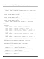
# Areas file for GRID / DOMAIN 1
#
# First the entire domain is selected and assigned to subdomain 1.
AREAS
AREA 1
SUBDOMAIN 1
MNMNBOX = (-10,-10)(99,99)
# Then the right hand part is removed from subdomain 1, by assigning
it
# to the inactive part "-1" of the domain.
AREA 2
SUBDOMAIN -1
ENCLOSURE =
(16,21)(16,17)(5,17)(5,5)(23,5)(23,1)(99,1)(99,21)(16,21)
Version 2.20, June 2011
27
User’s Guide for Parallel WAQUA/TRIWAQ and for Domain Decomposition
Figure 2.3: True (curvilinear) grid for domain/grid 1 of Figure 3. The strange part in the middle is
cut away via the areas-file (see text).
2.7
Format of the process configuration file
The format of the process configuration file used in domain decomposition with horizontal refinement is as follows (see Section 5.2.1 for an example):
DOMAINS
< DOMAIN=[ival]
GLOBAL
NAME = [text]
RUNID = [text]
EXPERIMENT = [text]
EXECUTABLE = [text], BUFSIZE=[ival]
CONFIG = [text]
DIRECTORY = [text]
SUBDOMAINS
< SUBDOMAIN = [ival]
EXECUTABLE = [text], BUFSIZE=[ival]
CONFIG = [text]
28
>
Chapter 2. Partitioning / Decomposition
>
OPTIONS
MATCH_ACCURACY = [rval]
VERBOSITY_LEVEL = [ival]
Explanation:
DOMAINS
DOMAIN
GLOBAL
NAME = [text]
RUNID = [text]
EXPERIMENT
[text]
EXECUTABLE
[text]
X1 Main keyword, indicating that a list of domains for domain decomposition with horizontal refinement follows.
M Main keyword, marking the start of the input for one domain
M Main keyword, marking the start of default values for the subdomains of the domain
M Logical name of the domain
M Code to identify input/output-files for the subdomains of a domain,
as used in the execution of the pre-processing stage of the computations (WAQPRE)
= O Name of the experiment (simulation) for a domain
= M
BUFSIZE=[ival]
O
CONFIG=[text]
M
DIRECTORY=[text]
O
OPTIONS
O
MATCH_ACCURACY D
= [rval]
VERBOSITY_LEVEL D
= [ival]
Name of the executable program to use for the simulation of the
subdomains of a domain. The name WAQPRO.EXE must be used
for all domains.
Buffer size (MW) for the executable. This option is read by the
run script and used to fill in the keyword CONFIG. The keyword
BUFSIZE is not read by the executable COEXEC.
EXECUTABLE and BUFSIZE must be specified on the same line.
Name of the file containing the name of the work directory and the
buffer size. This keyword is filled in by the run script and does not
have to be filled in by the user.
Directory where the waqpre SDS-file for the specific domain is
located.
Main keyword, start of the specification of options to executive
process COEXEC
Tolerance to be used in the comparison of real (x,y) coordinates
of the grids of different domains. Two grid points of different domains coincide when their distance in meters differs less than rval.
Default: 0.01 [m]
Amount of debug-output desired from the calculation regarding the
matching process of the domains. Default value is 8.
Note:
If you want to use Visipart for your DDHOR simulation then read Chapter 4 of the Visipart documentation. In this case there are some constraints for setting up your config file. Also an example
is placed how to use Visipart in combination with a DDHOR simulation.
Version 2.20, June 2011
29
User’s Guide for Parallel WAQUA/TRIWAQ and for Domain Decomposition
Quick Reference Auxiliary Programs for Coupled Simulations
2.8
The partitioner COPPRE
The partitioner is a program that is to be called after the preprocessor WAQPRE but before calling the parallel/domain decomposition version of WAQUA/TRIWAQ. It splits the SDS-file that has
been created by WAQPRE into several SDS-files, one for each subproblem. Each of the processes
in parallel WAQUA/TRIWAQ takes one of these subproblem SDS-files for input. The same holds
for TRIWAQ with domain decomposition, except that in that case WAQPRE is called multiple times
and that COPPRE each time extracts the SDS-file for one subproblem only.
2.8.1
Use of the partitioner COPPRE
In case of parallel runs, the partitioner is started by the run-procedure for the WAQUA/TRIWAQ
program WAQPRO.PL. This run-procedure is described in the User’s Guide WAQUA, in the section on Processor WAQPRO. In case of domain decomposition with horizontal or vertical refinement
COPPRE is started by the run-procedure for the program WAQPRE, which is described in User’s
Guide WAQUA, in the section on WAQPRE.
Input files:
COPPRE assumes that the following files are present:
SDS-<runid>
copcfg.gen.par
or
copcfg.gen.ddv
or
copcfg.gen.ddh
Partinputfile
or
Decomposit
coplds.waqua
30
The SDS-file that has been created by WAQPRE.
The configuration file for COPPRE (see Section 3), with separate
versions for parallel computing and domain decomposition with
vertical or horizontal refinement.
If the required file is not present in the working directory, it is
copied from the $SIMONADIR/bin directory. In parallel runs the
word %PARTIT% is replaced by the run-procedure in such a way
that the requested partitioning or partitioning-method is selected.
In domain decomposition runs the word %DECOMP% is replaced
by the name of the decomposition input file. Further in case of
vertical refinement the word %DOM% is replaced by the actual
subdomain number for which an SDS-file is to be created.
A so-called areas-file that contains a specification of the partitioning or domain decomposition. The former file needs only be
present if a manually created partitioning is to be used. For the
format of both files, see Section 2.6.
The specification of the LDS for TRIWAQ / WAQUA (see Chapter
4). If this file is not present in the working directory then a link is
created to this file in the $SIMONADIR/bin directory.
Chapter 2. Partitioning / Decomposition
coplds.svwp
SIMETF
simona.env
coppreref.arr
ldsref.arr
The specification of the LDS for SVWP (see Chapter 4). If not
present, the default version from the $SIMONADIR/bin directory
is used.
SIMONA error text file. If this file is not present in the working directory, a link is created to the SIMETF file in the $SIMONADIR/bin directory.
SIMONA environment file. If this file is not present in the working
directory, a link is created to the appropriate simona.env file in the
$SIMONADIR/bin directory.
Reference array for interpreting the configuration file (see Chapter
3). This file is expected in the $SIMONADIR/bin directory.
Reference array for interpreting the LDS specification files for
WAQUA/TRIWAQ and for SVWP (see Chapter 4). This file is
expected in the $SIMONADIR/bin directory.
Output files:
coppre-r.<runid>
SDS-<runid>-000
SDS-<runid>-<part>
Report file containing the partitioning.
SDS-file containing data (conversion tables) for the collector program.
SDS-files containing WAQUA/TRIWAQ input for subproblems,
one for each part/subdomain, and with <part> the part number in
three decimal digits.
COPPRE partitions experiment <expnam> in SDS-file SDS-<runid> into parts, according to the
directions given in the text file copcfg.inp (generated from generic input files copcfg.gen.par,
copcfg.gen.ddv and copcfg.gen.ddh by the run-procedures) that is formatted according to reference
array coppreref.arr. The contents of the SDS-file are specified in the file coplds.waqua, which is
formatted according to reference array ldsref.arr. If the experiment makes use of space varying
wind and pressure (SVWP), COPPRE determines the name and experiment of the SVWP SDS-file
from the SDS-file of the WAQUA/TRIWAQ experiment. The structure of the contents of the SVWP
file must be specified in the file coplds.svwp, which is also formatted according to reference array
ldsref.arr.
If in a parallel run the user does not want to use a COPPRE-internal partitioning method but wants
to provide the partitioning himself, then a filename should be given at the -partit option of the runprocedure WAQPRO.PL, partinputfile. This file should also be reachable for COPPRE. In domain
decomposition runs it makes no sense to use an automatic partitioning method for the complete domain, and a filename decomposit is required with the -decomp option of WAQPRE.PL in all cases.
However, the subdomains themselves can again be partitioned automatically which can be attractive
for large subdomains. This is a new feature of COPPRE that allows to enter an automatic partitioning method and a number of parts for each subdomain. Chapter 5 shows an example call of the run
procedures for this extended functionality.
COPPRE writes the partitioning to the file coppre-r.<runid>. This file is formatted in the same way
Version 2.20, June 2011
31
User’s Guide for Parallel WAQUA/TRIWAQ and for Domain Decomposition
as the input files in which a partitioning can be specified (see Section 2.6) and can be immediately
used with the -partit and -decomp options or imported in Visipart. It also gives some additional
information about the partitioning as comment.
The partitioner also creates a file with the name of the input SDS-file concatenated by ’-000’. This
file contains the data that is used by the partitioner itself and later on by the collector COPPOS.
The partitioner further produces files with names that are formed by the concatenation of the input SDS-filename and a number in the range 1 through the number of parts that is requested.
For instance, if the user requests a partitioning of SDS-file SDS-csm into 4 parts, then COPPRE
produces files SDS-csm-001 through SDS-csm-004. Each of these output files is a valid input
file for WAQUA/TRIWAQ. It does not contain data that is not relevant for the processing with
WAQUA/TRIWAQ (such as land boundary outlines, which are only used for post processing), hence
the files SDS-csm-001 through SDS-csm-004 can be used for computing with WAQUA/TRIWAQ
but not for post processing. In order to post process the data, it should first be assembled into a
single SDS-file using the postprocessor COPPOS.
If errors or warnings occur, COPPRE will give a short indication of the problem that was encountered.
The partitioner does not alter the original SDS-file in any way but merely copies its contents to the
subproblem SDS-files and makes the data consistent in the subproblem SDS-files.
Note: The LDS-description file coplds.waqua should be consistent with the version of WAQPRE
that is used for creation of the global SDS-file. No correct version of coplds.waqua exists for old
versions of WAQPRE (earlier than, say, 1998), since WAQPRE is extended with the creation of
additional data structures that are needed for distribution of WAQUA/TRIWAQ data.
Current Limitations
COPPRE only works for WAQUA/TRIWAQ input (possibly with SVWP data).
The maximum number of parts that can be requested is 999.
The output SDS-files will all be in the format of the system on which COPPRE runs. This means
that they cannot be used when instances of WAQUA/TRIWAQ in the parallel run are executing on
a system that uses a different format.
Only a fixed number of predefined MAPS is available (See keyword INDEXSETS, Section 4.2). If
new data structures are introduced in WAQUA/TRIWAQ, COPPRE will have to be extended. This
requires modifications on code-level.
32
Chapter 2. Partitioning / Decomposition
2.9
The MPI communication software
The communication between processes in a parallel run takes place through the MPI communication software, which supplies the basic data exchange operations. This section gives a brief outline
of working with MPI. For more details the user is referred to the MPI man pages, either locally or
on the Internet.
MPI is actually the (standardized) specification of an interface only, comparable to e.g. the Fortran
language specification. There are two versions of the standard: MPI-1 and MPI-2 (Fortran: 77,
90, 95 etc.). Parallel WAQUA uses features of MPI-1 only, although we might be using features of
MPI-2 in the future.
There are multiple implementations of the MPI-standards, comparable to different compilers for the
Fortran language. There are different general implementations, directed at multiple platforms, and
specific implementations that are optimized for one situation only. The most common versions are
MPICH, MPICH2 and LAM-MPI. Even most vendor-specific implementations, such as for Myrinet
or Infiniband communication networks are derived from adapting one of these implementations.
There are various differences between different MPI implementations. Especially the procedure to
start up the MPI communication system and to start programs are not well covered in the MPI standards. Where one implementation uses a command named "mpirun" another may use "mpiexec",
and yet another may require to first use "mpdboot" and then use "mpiexec". The appropriate commands for various MPI-implementations have been inserted in run-procedure WAQPRO.PL. They
are selected through environment-variable $MPI_VER, which is set through settings-file
$SIMONADIR/etc/-$UI_NAME/Settings.inc.
The most common MPI-implementation used for parallel WAQUA/TRIWAQ is at the moment
MPICH2. This implementation is also available on the MS Windows platform.
On Linux, the correct working of MPICH2 can be verified as follows:
• In the home-directory of each user who wants to use MPI, a file named ".mpd.conf" must
be created. This file must be readable for that user only ("chmod 600 .mpd.conf"). It must
contain a single line "secretword=simona".
• Create in a test-directory the file "mpd.hosts", with a list of machines to be used in a test (one
per line);
• Start a ring of MPI daemons with the command "mpdboot -n <nr> -f mpd.hosts -r rsh", with
<nr> the number of hosts in file mpd.hosts;
• Check whether the mpi-daemons are active through the command "mpdtrace";
• Stop all daemons through the command "mpdallexit".
Version 2.20, June 2011
33
User’s Guide for Parallel WAQUA/TRIWAQ and for Domain Decomposition
Note that WAQPRO.PL will start the MPI-subsystem before starting a parallel run. Therefore the
user should not start mpdboot himself. Also when python-processes are left over of previous usage
of MPICH2 this may hinder the starting of new parallel runs.
The installation and use of MPICH2 on the MS Windows platform is described in another document: the installation guide for parallel computing on XP (install.par-xp).
2.10
Start-up of coupled runs
The start-up of a coupled (parallel or domain decomposition) run is concerned with the following
aspects:
• Selecting the computing nodes (hosts) to be used by the run;
• Determining the mapping of computing processes (one instance of coexec.exe and an instance
of waqpro.exe per subdomain) over the available hosts;
• Starting the MPI-subsystem and starting the appropriate executables on the selected hosts.
These aspects are implemented through a "hostfile" and via the run-procedure WAQPRO.PL.
The selection of hosts may be done through a batch scheduling program, most notably the system
"PBS" (portable batch scheduler). On parallel computing systems that are governed by PBS the user
cannot start parallel runs directly, but must prepare a "job-script", then "submit a job", and then wait
until the job is handled by PBS. Under water PBS will wait until it has a sufficient number of the
requested type of computing nodes available and then allocate the nodes to the job and execute the
job-script. In this case the required hostfile is generated by PBS and read and used by WAQPRO.PL.
On systems where PBS is not used the user must prepare a hostfile for his coupled runs himself.
This is a simple file that must be called "hostfile.gen" and that must reside in the working directory for a run. It simply lists the host-names for the computing nodes to be used, plus optionally
the number of processing-units per host. A default-version is available in the "etc"-directory of a
SIMONA-installation, that is appropriate for stand-alone multi-processor or multi-core machines.
hostfile.gen
Configuration file used for determining a mapping of subdomains
onto hosts and for configuration of the MPI communication library.
If this file is not present in the working directory, it is created from
the hostfile.gen file in the $SIMONADIR/etc directory.
An example "hostfile.gen" is as follows:
34
Chapter 2. Partitioning / Decomposition
# this is a simple hostfile.gen that lists two machines:
linux101 ppn=2 # a dual-core machine
linux102 # a single-core machine (default ppn=1)
The mapping of subdomains (computing processes) onto hosts may be done by the user or may be
left to run-procedure WAQPRO.PL.
WAQPRO.PL implements two mapping mechanisms: Packed and Round-Robin, where Packed is
the default method.
The mapping Packed (with alias Compact) is useful for dual or quad cores in combination with the
partioning method strip, as it keeps as much as possible neighbouring processes on the same node to
minimize communications between nodes. It assumes that the number of processing units is equal
for all hosts, as many clusters have different queues such that within a queue all hosts have the same
characteristics (clockfrequency, number of cpus, etc).
An alternative to the Packed mapping mechanism is Round-Robin. Round-Robin mapping mechanism accounts for the number of processing units (processors/cores) of the different hosts as declared in the file "hostfile.gen". This mapping method consists of mapping subdomain 1 onto host
1, subdomain 2 onto host 2 and so on until host <nhosts>. In the second pass all hosts that have
at least 2 cpu’s are assigned a second subdomain. In the third pass hosts with at least 3 cpu’s get
another subdomain, and so on until all cpu’s of all hosts have gotten a subdomain to compute. If
there are still more subdomains then the whole process is repeated, starting with mapping the next
subdomain onto cpu 1 of host 1. Note that it is generally not advisable (as far as performance is
concerned) to assign more than one subdomain to a cpu.
Another alternative mechanism is to determine and prescribe the mapping yourself. For instance
when you have a domain decomposition run with in total 4 subdomains, you have two machines
"linux101" and "linux102" as described above, and you wish to place the smallest two subdomains,
numbers 1 and 3 onto the single-core machine "linux102". This is achieved with the option "hostmap 2,1,2,1" for WAQPRO.PL. This option maps the four subdomains onto the 2nd, 1st, 2nd
and 1st hosts of the hostfile respectively.
When running 4 processes on two dual cores, -hostmap Round-Robin is equal to -hostmap 1,2,1,2,
where -hostmap Packed is equal to -hostmap 1,1,2,2.
One important aspect of the hostfile as far as mapping is concerned is that the execution host, i.e.
the machine where you are logged in for starting a run (PBS: the machine where your job-script is
started), will be placed first in the hostfile by WAQPRO.PL. When you log-in on machine "linux102"
and start WAQPRO.PL, the order of the two machines in the hostfile will be interchanged. This is
done before the mapping is interpreted, and thus affects the meaning of the hostmap-option. This
may be avoided easily by adjusting the hostfile yourself such that the machine that you are logged
Version 2.20, June 2011
35
User’s Guide for Parallel WAQUA/TRIWAQ and for Domain Decomposition
in on is the first host.
The third aspect of starting a coupled run is concerned with starting MPI and starting the computing
processes needed for the run on the appropriate hosts. This is handled completely by WAQPRO.PL.
This run-procedure knows how to create the appropriate start-up commands for different MPIimplementations. It creates an appropriate start-command or an appropriate configuration-file and
then starts MPI.
2.11
The control program COEXEC
The executive/master process COEXEC is a process that starts and manages the parallel execution.
After its invocation by the user, it reads an input file that describes the processes used and their arguments. In case of a domain decomposition run with horizontal refinement it checks the consistency
of the different global domains with each other and the matching of the different computational
grids. After that it waits until the worker processes are finished or until an error occurs somewhere.
At that point it terminates the coupled run in an elegant way if possible.
2.11.1
Use of the control program COEXEC
COEXEC is started in the second phase of parallel runs (PRO) by the run-procedure for the WAQUA/
TRIWAQ program WAQPRO.PL. This run-procedure is described in the User’s Guide WAQUA, in
the section on Processor WAQPRO.
Input files:
COEXEC assumes that the following files are present:
proc_cfg.inp
SIMETF
simona.env
Process configuration file, a textual input file with specific information about the processes used in the coupled run. This file is generated automatically by the run-procedure in case of parallel runs
or when using domain decomposition with vertical refinement, and
must be provided by the user in case of horizontal refinement.
SIMONA error text file. If this file is not present in the working directory, a link is created to the SIMETF file in the $SIMONADIR/
etc/$UI_NAME directory.
SIMONA environment. If this file is not present in the working directory, a link is created to the simona.env file in the
$SIMONADIR/etc/-$UI_NAME directory.
Further COEXEC requires that an MPI-ring be started that is exclusively available to the current
coupled simulation. For this the run-procedure WAQPRO.PL, generates an appropriate configura36
Chapter 2. Partitioning / Decomposition
tion file and starts MPI. This procedure uses the file hostfile.gen, see Section 2.10.
The worker processes execute the WAQUA/ TRIWAQ executable using the SDS-file for the part
that is specified by COEXEC. The name of the SDS files is SDS-<runid>-<part> where <part> is
the three-digit number of each part and <runid> is the run-identification of each global domain.
The partitioner COPPRE creates these files. They should be located in the working directory of the
processor on which the WAQUA/TRIWAQ instance runs. Each worker process produces its own
report print file in the working directory.
Note that in case the disks of the processors that are involved in the parallel run are not mounted, then
it will be necessary to explicitly move the worker SDS-files to the disks where they are needed prior
to calling COEXEC. This is not supported by the standard procedure implemented in WAQPRO.PL.
Once the worker processes have started, the COEXEC process starts to wait for messages from the
worker processes. Such messages can be either output from the worker process or control messages.
Output from worker processes is simply forwarded to standard output and supplied with an extra
tag to mark which process has produced the output. Therefore, all lines of output start with the
processor number followed by a ’#’. The master processes control messages in an appropriate way.
After all worker processes have terminated, either because they are finished or because some error
has occurred, COEXEC closes the coupled run. File-I/O from the worker process goes directly to
disk, without interference of the master.
WAQPRO.PL will automatically start MPI, which is needed for the inter-process communication.
2.12
The collector COPPOS
After a parallel or domain decomposition run, the results of the computations are scattered over the
SDS-files of the subproblems. The collector COPPOS can be used to collect the results from the
subdomain SDS-files into the global SDS-file that was created by WAQPRE and then partitioned by
COPPRE. After running COPPOS on the subdomain SDS-files of a parallel run, the global SDS-file
contains the same information as when a sequential model run had taken place. In case of domain
decomposition with vertical refinement, the subdomain SDS-files use different numbers of layers.
In this case COPPOS converts the output data to the finest vertical resolution used using simple
(constant and linear) interpolation schemes. In case of horizontal refinement, part of the global domain may have been excluded from the simulation (marked inactive). In this part of field-arrays the
value 0.0 is stored, and the part is marked as dry land by setting screens.
2.12.1
Using the collector COPPOS
COPPOS is started in the third phase of parallel runs ("COL") by the run-procedure for the WAQUA/
TRIWAQ program WAQPRO.PL. This run-procedure is described in the User’s Guide WAQUA, in
Version 2.20, June 2011
37
User’s Guide for Parallel WAQUA/TRIWAQ and for Domain Decomposition
the section on Processor WAQPRO.
Input files:
COPPOS assumes that the following files are present:
SDS-<runid>
SDS-<runid>-000
SDS-<runid>-<part>
SIMETF
simona.env
The original SDS-file from which the subproblem SDS-files have
been created by COPPRE.
SDS-file created by COPPRE, which contains data for COEXEC
and COPPOS
SDS-files containing TRIWAQ output for subproblems, one for
each part/subdomain, and with <part> the part number in three
decimal digits.
SIMONA error text file. If this file is not present in the working directory, a link is created to the SIMETF file in the $SIMONADIR/bin directory.
SIMONA environment file. If this file is not present in the working directory, a link is created to the simona.env file in the $SIMONADIR/bin directory.
COPPOS collects each instance of a time-dependent array in the subdomain-files SDS-<runid><part> into a time-dependent array in the file SDS-<runid>. For example, if each of the subdomainfiles contains a time-dependent compound array SOLUTION_FLOW for time-instances 0.0 10.0
and 20.0 then after termination of COPPOS, the file SDS-<runid> contains the compound array
SOLUTION_FLOW for these same time-instances. COPPOS also collects time-independent arrays
that have been created at run-time if they are marked properly in the LDS description file (see
Section 4.3). Finally COPPOS creates the stand-alone array POWNER, in which the partitioning of
the WAQUA mesh into subdomains is stored that was used in the simulation.
38
Chapter 3. The configuration file for the partitioner COPPRE
Chapter 3
The configuration file for the partitioner
COPPRE
The configuration for COPPRE is specified in an input file. This input file is structures according
to SIMONA input files and has two main keywords: PARTITIONING and MACHINE. These keywords will be discussed below. An example can be found in Section 5.2.3.
3.1
PARTITIONING (mandatory)
A partitioning for domain decomposition or parallel computing can be specified in three ways: using an automatic partitioning method, via the areas format and via the value (part number) for each
grid point. Further some options can be set that affect the behavior of the partitioner.
PARTITIONING
| AREAS
AREA [iseq]
SUBDOMAIN = [ival]
| <MNMNBOX ([ival1],[ival2])([ival3],[ival4])>
<
| ENCLOSURE <([ival1],[ival2])>
<
| PART_VALUES
GLOBAL
LOCAL
| PARTMETHOD
Version 2.20, June 2011
39
User’s Guide for Parallel WAQUA/TRIWAQ and for Domain Decomposition
NPART = [ival]
| STRIP = [ANY,ROW,COL]
<
| ORB = [ANY,ROW,COL]
<
| AUTOMATIC
SPLITDOM = [ival]
OPTIONS
TOFILE = [filename]
ONLYDOMS = <[ival]>
ONLYPARTS = <[ival]>
PARTONLY
ADD_GUARDB
GUARDB_WIDTH = [ival]
OPTIM
Explanation:
PARTMETHOD
O
NPART = [ival]
STRIP
M
X2
ORB
X2
AUTOMATIC
X2
AREAS
X1
PART_VALUES
X1
OPTIONS
O
40
Use of this keyword activates specification of the partitioning
via one of the automatic partitioning methods (default is AUTOMATIC)
Number of parts to be created
strip wise partitioning into NPART strips. This can be done in
columns or in rows. If ANY is specified, the partitioner will decide
which direction is most likely to be best. The argument is optional;
ANY is the default.
ORB partitioning into NPART parts. The first cut is made along
ROWS or COLUMNS depending on what is specified after this
keyword. If ANY is specified, the partitioner will decide for itself.
The argument is optional; ANY is the default.
Partitioning method that chooses between Strip Any and Orb Any
by minimizing the number of communication points.
Use of this keyword selects specification of the decomposition via
the areas-construction, i.e. as a sequence of areas that are each
assigned to a part, see Section 2.6.
Use of this keyword selects specification of the partitioning by giving the part number for each grid point using the SIMONA box
format, see Section 2.6.
This keyword starts the options section of the partitioning configuration
Chapter 3. The configuration file for the partitioner COPPRE
TOFILE =[filename]
O
ONLYDOMS
<[ival]>
= O
ONLYPARTS
<[ival]>
PARTONLY
<[ival]>
= O
= D
ADD_GUARDB
D
GUARDB_WIDTH
D
OPTIM
D
Write the partitioning to file filename. Usually, this option will not
be necessary as the report file also contains the partitioning in a
suitable format
Create SDS-files only for all parts of the specified but still unsplitted subdomains. This option is incompatible with the ONLYPARTS and PARTONLY option.
Create SDS-files only for the specified parts. This option is incompatible with the ONLYDOMS and PARTONLY option.
If this keyword is set, COPPRE will only perform the partitioning
and write the report file, but not produce subdomain SDS-files.
This option is incompatible with the ONLYDOMS and ONLYPARTS option.
If this keyword is given, COPPRE ensures that there is enough
space around the entire mesh of the global domain needed for the
"guard band" in simulations with horizontal refinement, by adding
additional grid rows and columns where needed.
The number of grid rows and columns needed around each subdomain for communication with neighboring subdomains. Default=3, which is sufficient for parallel computing and vertical
refinement. However, 4 additional rows/columns are needed in
case of horizontal refinement, therefore this option is given in file
copcfg.gen.ddh.
Not used.
Note: besides the options that are shown, also the keyword OPTIM may be given. This keyword
was previously used for the level of automatic optimization of the initial partitioning. However, no
optimizations are currently available, therefore the keyword OPTIM currently has no effect.
Version 2.20, June 2011
41
User’s Guide for Parallel WAQUA/TRIWAQ and for Domain Decomposition
3.2
MACHINE (optional)
The machine keyword specifies the details of the architecture of the system on which parallel
WAQUA/TRIWAQ will run. It is currently only being used to perform optimizations (for nonzero optimization level, see Section 3.1 above).
MACHINE
NPROC = [ival]
TYPE = [CRAYT3E ,NOW ,SMP]
PSPEEDS
<PROC = [ival]
SPEED = [ival]>
CSPEEDS
< CONNECTION
PROCA = [ival]
PROCB = [ival]
SPEED = [ival] >
MACHINE
NPROC = [ival]
TYPE
O
M
O
PSPEEDS
PROC = [ival]
O
M
SPEED = [ival]
M
CSPEEDS
CONNECTION
PROCA = [ival]
PROCB = [ival]
O
O
M
M
SPEED = [ival]
M
42
Main keyword for specifying the system architecture
The total number of processors in the system
The system architecture. Currently supported types are the
CrayT3E, a network of workstations (NOW) and a symmetric multiprocessor (SMP) architecture.
List of non-default processor speeds.
Number ival of the processor with non-default speed. The numbering is arbitrary. At runtime, the master process COEXEC will
try and match the description of the architecture that is given here
in the input file with the system that it actually finds and use the
numbering as defined here.
Speed ival of the processor with non-default speed in % of the
default (i.e. default is 100)
List of non-default connection speeds.
The specification of a new connection starts with this keyword
Number ival of processor at the beginning of the link.
Number ival of processor at the end of the link; links
are undirected, hence link (PROCA,PROCB) is the same as
(PROCB,PROCA).
Speed ival of the link with non-default speed in % of the default
(i.e. default is 100)
Chapter 4. Specifying the data structure
Chapter 4
Specifying the data structure
In order to distribute and collect the data in the SDS-file, the partitioner and collector must know
which data there is, and how it is organized. This information is provided through the LDS description file. This file should remain fixed for one particular version of the LDS, but future developments
on WAQUA/TRIWAQ may require modifications. This chapter describes the organization of the file.
It has three main keywords: PARAMETERS, INDEXSETS and LDSDESCRIPTION. An example
can be found in Section 5.5.
4.1
PARAMETERS (Optional)
This keyword allows to define parameters, which may be used in the definition of index sets.
PARAMETERS
<PARAMETER
NAME =[text]
VALUE = [text]
>
PARAMETER
NAME = [text]
VALUE = [text]
Version 2.20, June 2011
R
M
M
This defines a new parameter with the specified name and value
Specifies the name of the parameter
Specifies the value of the parameter. The can be specified either
directly (e.g. ’3’ or ’55’), as an expression of other parameter values, or via an array-reference (e.g. ’MESH_IDIMEN(5)’). In the
latter case text should consist of a characteristic array name (e.g.
MESH_IDIMEN) plus the index within the array between parentheses (e.g. ’(5)’).
43
User’s Guide for Parallel WAQUA/TRIWAQ and for Domain Decomposition
4.2
INDEXSETS (Mandatory)
This keyword specifies which index sets there are. To understand the concept op an index set, consider for instance an array like IROGEO, which has size 3x(NOROWS+NOCOLS). Hence, indexing
in this array can be from 1 through 3 in the vertical direction and from 1 through NOROWS and
then from 1 through NOCOLS in the horizontal direction. In this case, the vertical direction is said
to have index set [1,3] and the horizontal direction is said to be the concatenation of the index-sets
NOROWS and NOCOLS, which run over [1,NOROWS] and [1,NOCOLS] respectively. Index sets
can be distributed or replicated. If they are replicated, then each subdomain will have the full index
set. If it is distributed, then each subdomain will only have the part of the index set that relates to its
own domain.
The format of the keyword is:
INDEXSETS
<INDSET
DEFINE
NAME = [text]
| DIRECT
CARDINALITY = [text]
| REPLICATE
<
| DISTRIBUTE_USING
MAP = [ival]
<
| INDIRECT
DEFINITION = [text]
COLLECT_USING
INTERP = [ival]
>
INDSET
DEFINE
NAME = [text]
DIRECT
44
R
M
M
X1
Specifies one index set
Starts the definition of the index set
The name of the index set, which is free to choose
Starts direct specification of the characteristics of the index set
Chapter 4. Specifying the data structure
CARDINALITY
[text]
= M
Specifies the number of elements in the index set (the cardinality
of the index set). This can be specified either directly (e.g. ’3’ or
’55’), through the value of a parameter, or via an array-reference
(e.g. ’MESH_IDIMEN(5)’). In the latter case text should consist
of a characteristic array name (e.g. MESH_IDIMEN) plus the index within the array between parentheses (e.g. ’(5)’).
REPLICATE
X2 Indicates that the index set must be replicated over the subproblems
(i.e. each subproblem gets a copy of the full index set plus the
associated values). If followed by the keyword MAP (see below)
then MAP is ignored.
DISTRIBUTE_USING X2 Indicates that the index set must be distributed over the subproblems. If this keyword is specified, the keyword MAP is also expected. If not, a warning occurs.
MAP = [ival]
O Selects the built-in local-to-global conversion table with specified
number for finding the global index that belongs to a local index
in a subproblem. Must be specified for distributed index sets, and
is ignored for replicated index sets. The list of built-in conversion
tables (i.e. the valid values for ival) can be found in the specification of the internal data structure (LDS) for COPPRE. (SIMONA
report lds_couple)
INDIRECT
X1 Starts indirect specification of the characteristics of the index set,
i.e. via references to other index sets.
DEFINITION = [text] M Expression, combination of other index sets.
COLLECT_USING
O Indicates that interpolation may be used in the conversion from one
(source) cardinality value to another (target) value.
INTERP = [ival]
M Selects the built-in interpolation method with specified number.
The list of available values is given in the specification of the
internal data structure (LDS) for COPPRE. (SIMONA report
lds_couple)
Example:
PARAMETERS
PARAMETER NAME=’KMAX’, VALUE=’MESH_IDIMEN(18)’
INDEXSETS
INDSET DEFINE NAME = ’KMAX ’,
DIRECT: (CARD =’KMAX’, REPLICATE)
INDSET DEFINE NAME = ’KMAX0’,
INDIRECT: (DEFINITION = ’1+KMAX’, COLLECT_USING 3)
INDSET DEFINE NAME=’MNMAXK’
DIRECT: ( CARD =’MESH_IDIMEN(5)’ , DISTRIBUTE, MAP=3 )
Version 2.20, June 2011
45
User’s Guide for Parallel WAQUA/TRIWAQ and for Domain Decomposition
INDSET DEFINE NAME=’NOTGWN’ ,
DIRECT: (CARD =’COEFF_GENERAL_ICGENA(1)’ , REPLICATE)
This example specifies one parameter with the name ’KMAX’ and value read from the 18th element
of the MESH_IDIMEN array, which is assumed to exist in the LDS. This parameter is used in the
definition of the first index set, also with name ’KMAX’. This first index set is replicated over the
subproblems. This means that all subproblems will have an index set KMAX of the same size as the
index set KMAX for the original problem. Arrays that refer to this index set (e.g. MESH_HLAY)
are simply copied into each subproblem.
The second index set ’KMAX0’ is an indirect one, which means that it is created by combination of
other index sets. In this case the definition is ’1+KMAX’, which combines the unnamed (implicit,
replicated) index set ’1’ with the index set ’KMAX’ by concatenation. The new index set ’KMAX0’
is given a special treatment during the collecting phase by selection of interpolation method 3.
The third index set, named ’MNMAXK’, has its cardinality stored in MESH_IDIMEN(5) and it
must be distributed using the internal local-to-global conversion table number 3. The fourth index
set is named ’NOTGWN’, its cardinality is found in the LDS-array ’COEFF_GENERAL_ICGENA’
at location 1. It must be replicated in all subproblems.
4.3
LDSDESC (mandatory)
This keyword specifies the contents and structure of the LDS, which consists of a number of compound arrays and a number of data arrays. If a data array is standalone, then it also occurs as a
compound array. The description of the LDS makes use of the index-sets that have been specified
in the keyword INDEXSETS.
LDSDESC
COMPOUNDS
<CMPND
CHNAME = [text]
NUMBER = [ival]
NLEVEL = [ival]
NTIME = [ival]
>
ARRAYS
<ARR
46
Chapter 4. Specifying the data structure
CHNAME = [text]
TYPE = [ival]
ADDRESS = <[ival]>
INDSET = [text]
>
COMPOUNDS
CMPND
CHNAME = [text]
NUMBER = [ival]
M
R
M
M
NLEVEL = [ival]
M
NTIME = [ival]
O
ARRAYS
ARR
CHNAME = [text]
TYPE = [text]
M
R
M
M
ADDRESS = <[ival]>
M
Version 2.20, June 2011
Start specification of compounds.
Specification of one compound.
Characteristic name of compound.
Number of the compound. If the largest number that is specified
here is ncmpnd then exactly ncmpnd occurrences of CMPND are
expected and all values in [1,ncmpnd] must be used. This number
is to be used below for specifying the locations of data arrays.
Number of sublevels under the root compound. This number is not
used and may be removed later on.
Flag to denote that the compound is time-dependent. If it is larger
than zero, then the array is assumed to be time-dependent and
COPPRE and COPPOS will determine the number of times for
themselves. A value less than zero signals that the array is timeindependent but will be created at runtime by TRIWAQ. So it is not
present at input, but must be collected after processing. If this keyword is omitted, the compound is assumed to be time-independent
and will not be collected.
Start specification of data arrays.
Specification of one data array.
Characteristic name of data array.
textual specification of the type of the data array. This can be any
of INT, REAL, CHAR*yy, DOUBLE, where yy is the length of
the character strings concerned, such as 80 or 128.
Path to the leaf array. This is the SIMONA level-path of an array relative to the compound array to which it belongs, see the
SIMONA Programmer’s Guide, paragraph 7.1.4 (SIMONA report
90-09), and the specification of arrays in, e.g., LDS FLOW. Further
the address specified here contains in its first location the number
of the root compound to which the leaf array is attached.
47
User’s Guide for Parallel WAQUA/TRIWAQ and for Domain Decomposition
INDSET = [text]
M
Textual specification of the structure of the index set of the leaf
array. text may contain any of the following symbols :
+:
concatenation of two index sets
*:
Cartesian product of two index sets
(:
start specification of compound index set
):
end specification of compound index set
indset :
the name of an index set, which should occur
under the keyword INDEXSETS
ival :
the cardinality of an unnamed index set
max(a,b) : where a and b are index sets. This operator returns either a or b, whichever has the largest
cardinality. If both have the same cardinality, the operator returns the index set that is
compound (i.e. made up of several others) or
that is distributed according to the definition
of the index set after the main keyword INDEXSETS. If this still does not make a distinction between a and b, the operator returns
b.
For example, text = ‘12*MNMAXK*(4+KMAX)’ would specify
and index set comprised of the Cartesian product of an unnamed
index set with cardinality 12, the named index set MNMAXK and
the index set 4+KMAX, which is itself the concatenation of an
unnamed index set with cardinality 4 and the named index set
KMAX. This index set means that the corresponding array is threedimensional with sizes 12, mnmaxk and 4+kmax.
Second example: text = ‘2*max(1,NSRC)’ is equivalent to
‘2*NSRC‘ if NSRC has a cardinality larger than 1, and is equivalent to ‘2*1’ (or just ‘2’) otherwise.
The LDS is described as consisting of a number of trees, each with its own root, which is its toplevel (compound) array. The data arrays themselves are leafs of each tree. Some arrays can be both
root and leaf. In that case, it should appear both in the specification of the COMPOUNDS (i.e.
the root arrays) and in that of the ARRAYS (i.e. the leaf arrays). The intermediary parts of each
tree (i.e. the parts that are neither root nor leaf) are implicit in the ADDRESS specification of the
ARRAYS.
Example:
LDSDEScription
COMPOUnds
CMPNd (CHNAme = ’MESH’, NUMBer = 1, NLEVel = 1)
CMPNd (CHNAme = ’SOLUTION_DRYWET’, NUMBer = 2, NLEVel = 0)
CMPNd (CHNAme = ’LAYER_INTERFACES’, NUMBer = 3, NLEVel = 0)
48
Chapter 4. Specifying the data structure
CMPNd (CHNAme = ’CONTROL_PROCES’, NUMBer = 4, NLEVel = 0)
CMPNd (CHNAme = ’COEFF_GENERAL’, NUMBer = 5, NLEVel = 5)
ARRAYs
ARR (CHNAme=’MESH_IDIMEN’ ,TYPE=’INT’, ADDRess=1,2,1,
INDSet=’30’ )
ARR (CHNAme=’MESH_IOPEN’ ,TYPE=’INT’, ADDRess=1,2,4,
INDSet=’NTO*4’ )
ARR (CHNAme=’SOLUTION_DRYWET’,TYPE=’INT’, ADDRess=2 ,
INDSet=’MNMAXK’ )
This example specifies an LDS that consists of five root compound arrays, like ‘MESH’ and ‘SOLUTION_DRYWET’. There are only three leaf arrays specified here. The first is ‘MESH_IDIMEN’,
which is an integer array of length 30. It is part of the root compound ’MESH’ since the first
number in its address is 1, i.e. the number of root compound ‘MESH’. Under this compound,
‘MESH_IDIMEN’ is located at the first subbranch of the second main branch. The third array, ‘SOLUTION_DRYWET’ is both a root compound and a leaf array. It is an integer array whose size is
equal to the cardinality of the MNMAXK index set (See the example of the INDEXSETS keyword
above).
In this example, the partitioner will expect that there is also an array with address (1,1), since it finds
a specification of an array at address (1,2,..). If an array at address (1,1) would not exist, then there
would be no need to start at the second branch. As there is no specification of an array with address
(1,1) in this example, the partitioner will further ignore the address (1,1).
Version 2.20, June 2011
49
User’s Guide for Parallel WAQUA/TRIWAQ and for Domain Decomposition
Chapter 5
Examples
5.1
Examples for domain decomposition with vertical refinement
Below a small incomplete siminp-file is shown that forms the basis of the examples for domain decomposition with vertical refinement. A complete input-file can be found at the path examples/triwaqexamples/ddv-bakken. For simulation it is required to use a complete siminp-file.
5.1.1
Example SIMINP file for domain decomposition with vertical refinement
--#
# file siminp.bak.ddv
#
IDENTification
# programmanaam:
TRIWAQ
EXPERIMENT=’bak’ OVERWRITE
MODID=’DDvert’
TITLE=’DDvert Test
# end identification
MESH
GRID
50
Chapter 5. Examples
AREA(MMAX= 30, NMAX= 3, KMAX=
ANGLEgrid= 0.00, LATItude= 0.000)
# rechthoekig rooster
POINTS
# voor open randen:
P 1=(M= 1, N= 2, NAME=’Open Links’)
P 2=(M= 30, N= 2, NAME=’Open Rechts’)
# voor controle stations:
P 3=(M= 5, N= 2, NAME=’( 5, 2)’)
P 4=(M= 10, N= 2, NAME=’(10, 2)’)
P 5=(M= 15, N= 2, NAME=’(15, 2)’)
P 6=(M= 20, N= 2, NAME=’(20, 2)’)
P 7=(M= 25, N= 2, NAME=’(25, 2)’)
# definitie randen:
BOUNdaries
# polygonen computational grid enclosure:
ENCLOSURES
E: COORdinates=
( 1, 1) ( 30, 1) ( 30, 3) ( 1, 3) ( 1, 1)
# definitie open randen:
OPENings
OPEN 1=LINE(P 1, P 1, ’Open rand links’)
BATHYMETRY
GLOBAL
CONST_values = 4.00
DEPMULTiplier= 1.00, THREShold= 0.30, LAYOUT=1
DEPDEF= 9.00
VERTICAL
INCLUDE ’layer_def.
# end mesh
GENERAL
DIFFusion
Version 2.20, June 2011
51
User’s Guide for Parallel WAQUA/TRIWAQ and for Domain Decomposition
GLOBAL: CONST_value= 10.000
PHYSical_parameters
# zwaartekrachtsversnelling en dichtheden:
GRAVity=9.8130, WATDENsity= 1023.0, AIRDENsity= 1.2050
WIND
# wind gegevens:
WSTRESScoefficient= 0.00260, WCONVersionfactor= 0.51440, WUNIT=’KNOT’
# opgave global windsnelheid en richting:
WSPEED= 0.00, WANGLE= 0.00
# end general
---
5.1.2
Example include files for vertical refinement
--#
# file layer_def.1
#
LAYER = 1 :
THICKNess = 20 PERC
LAYER = 2 :
THICKNess = 80 PERC
LAYER = 3 :
THICKNess = 0.20 M
----#
# file layer_def.2
#
LAYER = 1 :
THICKNess = 6 PERC
LAYER = 2 :
THICKNess = 14 PERC
LAYER = 3 :
THICKNess = 20 PERC
LAYER = 4 :
THICKNess = 40 PERC
LAYER = 5 :
THICKNess = 20 PERC
LAYER = 6 :
THICKNess = 0.15 M
52
Chapter 5. Examples
LAYER = 7 :
THICKNess = 0.05 M
---
5.1.3
Example areas file for vertical refinement
Note that this file can also be used in case of horizontal refinement
--#
# file decomp.areas
#
AREAS
AREA 1
SUBDOMAIN 1
MNMN = ( 1, 1) (15, 3)
AREA 2
SUBDOMAIN 2
MNMN = (16, 1) (30, 3)
---
5.1.4
Example call of the run procedures for vertical refinement
--waqpre.pl -runid dd -input siminp.bak.dd -bufsize 10 -back n \
-ndom 2 -kmax 3,7 -decomp decomp.areas -buf_prt 5
waqpro.pl -runid dd -ndom 2 -bufsize 4,5 -buf_prt 5 -buf_exc 5 \
-back no
---
5.1.5
Example call for vertical refinement using automatic partitioning
--waqpre.pl -runid dd -input siminp.bak.dd -bufsize 10 -back n \
-ndom 2 -kmax 3,7 -decomp decomp.areas -buf_prt 5 \
Version 2.20, June 2011
53
User’s Guide for Parallel WAQUA/TRIWAQ and for Domain Decomposition
-npart 1,3 -partit -,orb_row
waqpro.pl -runid dd -ndom 4 -bufsize 4,5 -buf_prt 5 -buf_exc 5 \
-back no
---
5.2
Examples for domain decomposition with horizontal refinement
5.2.1
Example process configuration file for horizontal refinement
--DOMAINS
D 1
GLOBAL
NAME=’Rymamo’, RUNID=’rym’, EXP=’rym’,
EXEC=’waqpro.exe’, BUFSize=20
D 2
GLOBAL
NAME=’Kuststrook’, RUNID=’kust’, EXP=’k90’,
EXEC=’waqpro.exe’, BUFSize=10
---
5.2.2
Example call of the run-procedures for horizontal refinement
--waqpre.pl -runid rym -input siminp.rymamo -bufsize 10 -back n \
-decomp decomp.rymamo -buf_prt 5
waqpre.pl -runid kust -input siminp.kuststr90 -bufsize 10 -back n \
-decomp decomp.kust -buf_prt 5
waqpro.pl -runid kust_rym -config proc_cfg.kust_rym -check_only no -back
no
---
54
Chapter 5. Examples
5.2.3
Example for horizontal refinement using automatic partitioning
--waqpre.pl -runid rym -input siminp.rymamo -bufsize 10 -back n \
-decomp decomp.rymamo -buf_prt 5 -npart 4 -partit strip
waqpre.pl -runid kust -input siminp.kuststr90 -bufsize 10 -back n \
-decomp decomp.kust -buf_prt 5 -npart 2 -partit orb_col
waqpro.pl -runid kust_rym -config proc_cfg.kust_rym \
-check_only no -back no \
-decomp decomp.rymamo -buf_prt 5
---
5.3
Example partitioner configuration file
The following file gives an example of a file that gives the configuration for COPPRE (see Chapter
3). Usually, the user will not create this file, but use the default files copcfg.gen.par, copcfg.gen.ddv
and copcfg.gen.ddh from the bin-directory of the installation. These default files are automatically
used by the run procedures.
The file specifies that the grid is to be partitioned into 2 parts, using the ORB method. Since the
direction of the first cut is not mentioned, the partitioner COPPRE will decide for itself. In this
configuration file, the user specifies that only the partitioning must be done (PARTONLY) but not
the splitting of the SDS-file. Possibly, the user will want to modify the partitioning that is written to
the report file and then do the splitting with the modified partitioning later on.
The MACHINE keyword here specifies that the target platform is an SMP system with 2 processors.
The first of the two processors is only half as fast as the other one. The specification of the connection speed is not useful here, because there is just one link and the partitioner uses only relative
speeds, no absolute speeds.
--#----------------------------------------------#
# copcfg.gen.par - Default Partitioning Configuration for parallel
# computations
#
#----------------------------------------------Version 2.20, June 2011
55
User’s Guide for Parallel WAQUA/TRIWAQ and for Domain Decomposition
#
# Configuration of the desired partitioning of the WAQUA/TRIWAQ grid:
#
PARTITIONING
#
# * PARTMETHOD: Select a partitioning method.
#
PARTMETHOD
NPART: 2
ORB
#
# * PART_VALUES: Use a manually created partitioning.
# INCLUDE ’somefile.partit’
#
# Partitioning options:
#
OPTIONS
PARTONLY
#
# * MACHINE: description of the target parallel computer
# for the parallel run.
#
MACHINE
#
# * TYPE: system architecture.
#
Valid types are:
SMP, CRAYT3E, NOW
TYPE : SMP
#
# * NPROC: number of processors in parallel computer
#
NPROC = 2
#
# * PSPEED: list of non-default processor speeds in
56
Chapter 5. Examples
# default speed = 100
#
PSPEED
PROC 1 :
SPEED = 50
---
5.4
Example partitioning Input file
The following is an example of a partitioning input file for using manually created or improved partitionings (see also Section 2.6). Note that this type of file is also automatically written to the report
file and can be read by auxiliary program Visipart, for inspecting and optimizing grid partitionings.
Each nonzero value denotes the number of the part to which the corresponding (m,n) point is assigned. By changing this value, the assignment of the point is changed. In this way, the user can
modify the partitioning. In this example part-numbers are listed for (open and closed) boundary
points too. The partitioner COPPRE ignores these values and will determine an appropriate partitioning for the boundary points itself.
--#
# PARTITIONING FILE
#
# DATE/TIME: 14-Jan-1999 09:49:52
#
# Part 1 contains 285 nodes and has neighbours (intfsize):
# 2 ( 59) 3 ( 24)
# Part 2 contains 295 nodes and has neighbours (intfsize):
# 1 ( 73) 3 ( 44)
# Part 3 contains 222 nodes and has neighbours (intfsize):
# 1 ( 17) 2 ( 39) 4 ( 25)
# Part 4 contains 211 nodes and has neighbours (intfsize):
# 3 ( 27)
#
#
PART_VALUES
Version 2.20, June 2011
57
User’s Guide for Parallel WAQUA/TRIWAQ and for Domain Decomposition
GLOBAL
LAYOUT = 1
LOCAL
BOX MNMN = ( 1, 1)( 72, 19)
VARIABLEVALUES
0
0
0
0
0
0
0
0
0
0
0
0
0
0
0
0
0
0
0
0
1
1
1
1
1
1
1
1
0
0
0
0
0
0
0
0
0
0
0
58
0
1
1
1
1
1
1
0
0
0
0
0
0
0
0
0
0
0
1
1
1
1
1
1
1
1
1
1
1
0
0
0
0
0
0
0
0
0
0
0
1
1
1
1
1
1
1
1
0
0
0
0
0
0
0
0
0
1
1
1
1
1
1
1
1
1
1
1
1
1
1
0
0
0
0
0
0
0
0
1
1
1
1
1
1
1
1
1
1
0
0
0
0
0
0
1
1
1
1
1
1
1
1
1
1
1
1
1
1
1
0
0
0
0
0
0
0
0
1
1
1
1
1
1
1
1
1
1
1
1
0
1
1
1
1
1
1
1
1
1
1
1
1
1
1
1
1
1
1
1
0
0
0
0
0
0
0
1
1
1
1
1
1
1
1
1
1
1
1
1
1
1
1
1
1
1
1
1
1
1
1
1
1
1
1
1
1
1
1
0
0
0
0
0
0
0
1
1
1
1
1
1
1
1
1
1
1
1
1
1
1
1
1
1
1
1
1
1
1
1
1
1
1
1
1
1
1
1
1
1
1
1
0
0
0
1
1
1
1
1
1
1
1
1
1
1
1
1
1
1
1
1
1
1
1
1
1
1
0
0
0
0
0
1
1
1
1
1
1
1
1
1
3
0
1
1
1
1
1
1
1
1
1
1
1
1
1
1
1
1
1
1
1
1
1
1
0
0
0
0
0
0
0
0
0
0
1
1
1
1
1
3
0
0
0
1
1
1
1
1
1
1
1
1
1
1
1
1
1
1
1
1
1
1
1
0
0
0
0
0
0
0
0
0
0
1
1
1
1
1
3
0
0
0
0
0
1
1
1
1
1
1
1
1
1
1
1
1
1
1
1
1
1
0
0
0
0
0
0
0
0
0
0
1
1
1
1
1
1
3
0
0
0
0
0
0
0
2
2
2
2
2
2
2
2
2
2
2
2
2
0
0
0
0
0
0
0
0
0
0
0
1
1
1
1
1
1
1
3
0
0
0
0
0
0
0
0
0
0
0
0
2
2
2
2
2
2
2
2
0
0
0
0
0
0
0
0
2
2
2
2
2
2
2
2
2
2
3
0
0
0
0
0
0
0
0
0
0
0
0
0
2
2
2
2
2
2
2
2
0
0
0
0
0
0
2
2
2
2
2
2
2
2
2
2
2
3
0
0
0
0
0
0
0
0
0
0
0
0
0
2
2
2
2
2
2
2
2
2
0
0
0
2
2
2
2
2
2
2
2
2
2
2
2
2
3
0
0
0
0
0
0
0
0
0
0
0
0
0
0
2
2
2
2
2
2
2
2
2
2
2
2
2
2
2
2
2
2
2
2
2
2
2
2
3
0
0
0
0
0
0
0
0
0
0
0
0
0
0
0
2
2
2
2
2
2
2
2
2
2
2
2
2
2
2
2
2
2
2
2
2
2
2
3
0
0
0
0
0
0
0
0
0
0
0
0
0
0
0
0
2
2
2
2
2
2
2
2
2
2
2
2
2
2
2
2
2
2
2
2
2
2
3
0
0
0
0
0
0
0
0
0
0
0
0
0
0
0
0
0
2
2
2
2
2
2
2
2
2
2
2
2
2
2
2
2
2
2
2
2
2
3
Chapter 5. Examples
0
0
0
0
0
0
0
0
0
0
0
0
0
0
0
0
0
0
0
0
0
0
0
0
0
0
0
0
0
0
0
0
0
0
0
0
0
0
0
0
0
0
0
0
0
0
0
0
0
0
0
0
0
0
0
0
0
0
0
0
0
0
0
0
0
0
0
0
0
0
0
0
0
0
0
0
0
0
0
0
0
0
0
0
0
0
0
0
0
0
0
0
0
0
0
0
0
0
0
0
0
0
0
0
0
0
0
0
0
0
0
0
0
0
0
0
0
0
0
0
0
0
0
0
0
0
0
0
0
0
0
0
0
0
0
0
0
0
0
0
0
0
0
0
0
0
0
0
0
0
0
0
0
0
0
0
0
0
0
0
0
0
0
0
0
0
0
0
0
0
0
0
0
0
0
0
0
0
0
0
0
0
0
0
0
0
0
0
0
0
0
0
0
0
0
0
0
0
0
0
0
0
0
0
0
0
0
0
0
0
0
0
0
0
0
0
0
0
0
0
0
0
0
0
0
0
0
0
0
0
0
3
3
0
0
0
3
3
3
3
3
0
0
0
0
0
0
0
0
0
0
0
0
0
0
0
0
0
0
0
0
0
0
0
3
3
3
3
3
3
3
3
3
3
3
0
0
0
0
0
0
0
0
0
0
0
0
0
0
0
0
0
0
0
0
0
0
3
3
3
3
3
3
3
3
3
3
3
3
3
3
0
0
0
0
0
0
0
0
0
0
0
0
0
0
0
0
0
0
0
BOX MNMN = ( 1, 20)( 72, 31)
0
0
0
0
0
0
0
0
0
0
Version 2.20, June 2011
0
0
0
0
0
0
0
0
0
0
0
0
0
0
0
0
0
0
0
0
0
0
0
0
0
0
0
0
0
0
0
0
0
0
0
0
0
0
0
0
3
3
3
3
3
3
3
3
3
3
3
3
3
3
3
3
0
0
0
0
0
0
0
0
0
0
0
0
0
0
0
0
0
3
3
3
3
3
3
3
3
3
3
3
3
3
3
3
3
3
4
0
0
0
0
0
0
0
0
0
0
0
0
0
0
0
3
3
3
3
3
3
3
3
3
3
3
3
3
3
3
3
3
4
4
4
4
0
0
0
0
0
0
0
0
0
0
0
0
3
3
3
3
3
3
3
3
3
3
3
3
3
3
3
3
3
4
4
4
4
4
4
4
0
0
0
0
0
0
0
0
0
3
3
3
3
3
3
3
3
3
3
3
3
3
3
3
3
3
4
4
4
4
4
4
4
4
0
0
0
0
0
0
0
0
3
3
3
3
3
3
3
3
3
3
3
3
3
3
3
3
3
4
4
4
4
4
4
4
4
4
4
4
0
0
0
0
0
3
3
3
3
3
3
3
3
3
3
3
3
3
3
3
3
3
4
4
4
4
4
4
4
4
4
4
4
4
0
0
0
0
3
3
3
3
3
3
3
3
3
3
3
3
3
3
3
3
3
4
4
4
4
4
4
4
4
4
4
4
4
4
0
0
0
3
3
3
3
3
3
3
3
3
3
3
3
3
3
3
3
3
4
4
4
4
4
4
4
4
4
4
4
4
4
0
0
0
VARIABLEVALUES
0
0
0
0
0
0
0
0
0
0
0
0
0
0
0
0
0
0
0
0
0
0
0
0
0
0
0
0
0
0
0
0
0
0
0
0
0
0
0
0
0
0
0
0
0
0
0
0
0
0
0
0
0
0
0
0
0
0
0
0
0
0
0
0
0
0
0
0
0
0
59
User’s Guide for Parallel WAQUA/TRIWAQ and for Domain Decomposition
0
0
0
0
0
0
2
2
2
2
2
2
2
2
2
2
2
2
2
2
2
2
2
2
2
2
2
2
3
3
3
3
3
3
3
3
0
0
0
0
0
0
0
0
0
60
0
0
0
0
0
0
2
2
2
2
2
2
2
2
2
2
2
2
2
2
2
2
2
2
2
2
2
2
3
3
3
3
3
3
0
0
0
0
0
0
0
0
0
0
0
0
0
0
0
0
0
2
2
2
2
2
2
2
2
2
2
2
2
2
2
2
2
2
2
2
2
2
2
3
3
3
3
3
0
0
0
0
0
0
0
0
0
0
0
0
0
0
0
0
0
0
0
2
2
2
2
2
2
2
2
2
2
2
2
2
2
2
2
2
2
2
2
2
3
3
3
3
0
0
0
0
0
0
0
0
0
0
0
0
0
0
0
0
0
0
0
0
0
2
2
2
2
2
2
2
2
2
2
2
2
2
2
2
2
2
2
2
2
3
3
0
0
0
0
0
0
0
0
0
0
0
0
0
0
0
0
0
0
0
0
0
0
0
0
0
0
0
0
2
2
2
2
2
2
2
2
2
2
2
2
2
2
0
0
0
0
0
0
0
0
0
0
0
0
0
0
0
0
0
0
0
0
0
0
0
0
0
0
0
0
0
0
0
0
0
0
0
2
2
2
2
2
2
2
2
2
0
0
0
0
0
0
0
0
0
0
0
0
0
0
0
0
0
0
0
0
0
0
0
0
0
0
0
0
0
0
0
0
0
0
0
0
0
2
2
2
0
0
0
0
0
0
0
0
0
0
0
0
0
0
0
0
0
0
0
0
0
0
0
0
0
0
0
0
0
0
0
0
0
0
0
0
0
0
0
0
0
0
0
0
0
0
0
0
0
0
0
0
0
0
0
0
0
0
0
0
0
0
0
0
0
0
0
0
0
0
0
0
0
0
0
0
0
0
0
0
0
0
0
0
0
0
0
0
0
0
0
0
0
0
0
0
0
0
0
0
0
0
0
0
0
0
0
0
0
0
0
0
0
0
0
0
0
0
0
0
0
0
0
0
0
0
0
0
0
0
0
0
0
0
0
0
0
0
0
0
0
0
0
0
0
0
0
0
0
0
0
0
0
0
0
0
0
0
0
0
0
0
0
0
0
0
0
0
0
0
0
0
0
0
0
0
0
0
0
0
0
0
0
0
0
0
0
0
0
0
0
0
0
0
0
0
0
0
0
0
0
0
0
0
Chapter 5. Examples
3
4
4
4
4
4
4
4
4
4
4
4
4
4
4
0
0
0
0
0
0
4
4
4
4
4
4
4
4
4
4
4
0
0
0
0
0
0
0
0
4
4
4
4
4
4
4
4
4
0
0
0
0
0
0
0
0
0
4
4
4
4
4
4
4
4
4
0
0
0
0
0
0
0
0
0
4
4
4
4
4
4
4
4
4
0
0
0
0
0
0
0
4
4
4
4
4
4
4
4
4
4
0
0
0
0
0
0
4
4
4
4
4
4
4
4
4
4
4
0
0
0
0
4
4
4
4
4
4
4
4
4
4
4
4
4
0
0
0
4
4
4
4
4
4
4
4
4
4
4
4
4
4
0
0
4
4
4
4
4
4
4
4
4
4
4
4
4
4
0
0
0
4
4
4
4
4
4
4
4
4
4
4
4
4
4
0
0
0
4
4
4
4
4
4
4
4
4
4
4
4
4
4
0
---
5.5
Example LDS description
The following is the LDS description for the SVWP LDS (see also Chapter 4). The LDS description
for WAQUA/TRIWAQ is substantially larger, but not essentially different.
--#
# coplds.svwp - Local Data Structure description for SVWP.
#
INDEXSETS
INDSET DEFINE NAME = ’MMAX ’,
DIRECT: (CARD =’MESH01_SPECIFIC_IDIMEN(1)’ , DISTRIBUTE,
MAP = 1 )
INDSET DEFINE NAME = ’NMAX ’,
DIRECT: (CARD =’MESH01_SPECIFIC_IDIMEN(2)’ , DISTRIBUTE,
MAP = 2 )
INDSET DEFINE NAME = ’NCHAR ’,
DIRECT: (CARD =’MESH01_GENERAL_DIMENSIONS(26)’, REPLICATE)
Version 2.20, June 2011
61
User’s Guide for Parallel WAQUA/TRIWAQ and for Domain Decomposition
INDSET DEFINE NAME = ’NSOLTP’,
DIRECT: (CARD =’PROBLEM01_GENERAL_GLOBAL(2)’ , REPLICATE)
INDSET DEFINE NAME = ’MAXFRE’,
DIRECT: (CARD =’PROBLEM01_GENERAL_GLOBAL(1)’ , REPLICATE)
INDSET DEFINE NAME = ’INPELM’,
DIRECT: (CARD =’MESH01_GENERAL_DIMENSIONS(10)’, REPLICATE)
INDSET DEFINE NAME = ’NCEL’ ,
DIRECT: (CARD =’MESH01_GENERAL_DIMENSIONS(7)’ , REPLICATE)
INDSET DEFINE NAME = ’NWTIM’ ,
DIRECT: (CARD =’CONTROL_SVWP_ICWINA(1)’ , REPLICATE)
LDSDESc
COMPOUNDS
CMPND (CHNAme = ’MESH’ ,NUMBER = 1, NLEVEL = 1)
CMPND (CHNAme = ’PROBLEM’ ,NUMBER = 2, NLEVEL = 1)
CMPND (CHNAme = ’CONTROL_SVWP’ ,NUMBER = 3, NLEVEL = 2)
CMPND (CHNAme = ’SOLUTION_WIND’ ,NUMBER = 4, NLEVEL = 0,
NTIME = 10)
CMPND (CHNAme = ’SOLUTION_PRESS’ ,NUMBER = 5, NLEVEL = 0,
NTIME = 10)
CMPND (CHNAme = ’COEFFICIENTS’ ,NUMBER = 6, NLEVEL = 0)
CMPND (CHNAme = ’IDENTIFICATION’ ,NUMBER = 7, NLEVEL = 0)
ARRAYS
ARR(CHNAme=’MESH01_GENERAL_DIMENSIONS’ ,TYPE=’INT’,
ADDRESS=1,1,1,1 ,INDSET=’80’ )
ARR(CHNAme=’MESH01_GENERAL_COOR’ ,TYPE=’REAL’,
ADDRESS=1,1,1,2 ,INDSET=’30’ )
ARR(CHNAme=’MESH01_GENERAL_KCEL’ ,TYPE=’INT’,
ADDRESS=1,1,1,4 ,INDSET=’INPELM*NCEL’ )
ARR(CHNAme=’MESH01_GENERAL_MESHNAMES’ ,TYPE=’CHAR*80’,
ADDRESS=1,1,1,9 ,INDSET=’NCHAR’ )
ARR(CHNAme=’MESH01_SPECIFIC_IDIMEN’ ,TYPE=’INT’,
ADDRESS=1,1,2 ,INDSET=’20’ )
62
Chapter 5. Examples
ARR(CHNAme=’PROBLEM01_GENERAL_GLOBAL’ ,TYPE=’INT’
ADDRESS=2,1,1,1 ,INDSET=’20’ )
ARR(CHNAme=’PROBLEM01_GENERAL_SOLUTIONTYPES’ ,TYPE=’INT’
ADDRESS=2,1,1,2 ,INDSET=’50*NSOLTP’ )
ARR(CHNAme=’PROBLEM01_GENERAL_FREEDOM’ ,TYPE=’INT’
ADDRESS=2,1,1,3 ,INDSET=’MAXFRE*NSOLTP’ )
ARR(CHNAme=’PROBLEM01_GENERAL_IFUNC’ ,TYPE=’INT’
ADDRESS=2,1,1,4 ,INDSET=’INPELM*MAXFRE*NSOLTP’ )
ARR(CHNAme=’CONTROL_SVWP_ICWINA’ ,TYPE=’INT’,
ADDRESS=3,1 ,INDSET=’20’ )
ARR(CHNAme=’CONTROL_SVWP_WINTIM’ ,TYPE=’REAL’,
ADDRESS=3,2 ,INDSET=’NWTIM’ )
ARR(CHNAme=’SOLUTION_WIND’ ,TYPE=’REAL’,
ADDRESS=4 ,INDSET=’MMAX*NMAX*2’ )
ARR(CHNAme=’SOLUTION_PRESS’ ,TYPE=’REAL’,
ADDRESS=5 ,INDSET=’MMAX*NMAX’ )
ARR(CHNAme=’COEFFICIENTS’ ,TYPE=’REAL’,
ADDRESS=6 ,INDSET=’20’ )
ARR(CHNAme=’IDENTIFICATION’ ,TYPE=’CHAR*80’,
ADDRESS=7 ,INDSET=’20’ )
Version 2.20, June 2011
63
Appendices
64
Appendix A. Glossary of terms
Appendix A
Glossary of terms
areas file
COEXEC
COPPOS
COPPRE
hostfile
MPI
ORB
Partitioning
PVM
Visipart
Version 2.20, June 2011
File specifying the decomposition of the grid into subdomains. See
Section 2.6 for a specification of the format and Section 5.1.3 for
an example.
Executive/master program that starts and controls a coupled run, in
which a number of WAQUA/TRIWAQ processes together execute
a simulation (see Section 2.11)
Program that collects the results of the subdomain computations
into an SDS-file for the complete domain (see Section 2.12). In
case of vertical refinement the number of layers in the resulting
SDS-file is the maximum of the number of layers of the subdomains. Results from coarser subdomains are interpolated to the
final SDS-file.
Program that splits an SDS-file into smaller SDS-files, one for each
subproblem that is solved in parallel (see Section 2.8).
A configuration-file specifying the hosts (computers) to be used in
a parallel/domain decomposition run and the number of processing
elements (cpu’s) per machine (see Section 2.10).
Message Passing Interface. An international standard for passing
messages between different Fortran and C programs. This is used
for communication in parallel WAQUA/TRIWAQ since SIMONA
version 2005-02 (see Section 2.9).
Orthogonal Recursive Bisection, a method to divide the problem
grid into subgrids (see Section 2.5.2).
Determining a splitting of the problem grid into subgrids (see
Chapter 2).
Parallel Virtual Machine. A combination of a run-time environment (a daemon) and a library of routines used to communicate
data between processes. Used for parallel WAQUA/TRIWAQ up
to SIMONA version 2005-01.
Graphical tool for creating and/or modifying grid partitionings for
parallel WAQUA/TRIWAQ and for domain decomposition.
I