Download SPOCS 6.0 User Guide

TNO Information and Communication Technology
Delft
Brassersplein 2
P.O. Box 5050
2600 GB Delft
The Nederlands
TNO Report
www.tno.nl
www.spocs.nl/eng
SPOCS 6.0
User Guide
Date
January 21, 2009
Title
Authors
Status
User Guide, version for SPOCS 6.0
Rob F.M. van den Brink, Hernán Córdova,
Released
All rights reserved.
No part of this publication may be reproduced and/or published by print, photoprint, microfilm or
any other means without the previous written consent of TNO.
In case this report was drafted on instructions, the rights and obligations of contracting parties
are subject to either the Standard Conditions for Research Instructions given to TNO, or the
relevant agreement concluded between the contracting parties. Submitting the report for
inspection to parties who have a direct interest is permitted.
© 2009 TNO
81Pages
TNO 2009 - SPOCS 6.0, User Guide
Table of Contents
TABLE OF CONTENTS..................................................................................................................... 2
LIST OF ABBREVIATIONS.............................................................................................................. 4
1
1.1
1.2
1.3
1.4
DISCLAIMER AND COPYRIGHTS....................................................................................... 5
Copyrights of SPOCS and associated libraries ............................................................................. 5
Disclaimer .................................................................................................................................. 5
Third party rights ........................................................................................................................ 5
Support....................................................................................................................................... 5
2
2.1
2.2
OVERVIEW OF THE CAPABILITIES OF THE TOOL ....................................................... 6
What is SPOCS about?................................................................................................................ 6
Using SPOCS as DSL Performance simulator ............................................................................. 7
2.2.1 Example 2: Spectral Management (SpM) Studies ............................................................... 7
2.2.2 Example 1: DSL deployment Studies.................................................................................. 8
Using SPOCS to create custom noise profiles for DSL testing ..................................................... 8
2.3.1 Example 1: DSL performance testing................................................................................. 8
2.3.2 Example 2: Product selection ............................................................................................ 8
2.3
3
3.1
3.2
3.3
QUICK START EXAMPLES .................................................................................................. 9
Loading a first example scenario ................................................................................................. 9
Generating my first noise profile (quickstart_1.ssf)...................................................................... 9
Generating my first performance prediction (SPOCS/full only).................................................. 11
4
4.1
4.2
DEFINING AND RUNNING SCENARIOS........................................................................... 15
Overview of the GUI................................................................................................................. 15
Defining a stress environment ................................................................................................... 16
4.2.1 Defining a loop topology ................................................................................................. 16
4.2.2 Defining crosstalk coupling in the loop............................................................................ 18
4.2.3 Selecting disturbers......................................................................................................... 20
4.2.4 Defining frequency range and count ................................................................................ 21
4.2.5 Defining sweeps (“k1”) and constants (“k2” and “k3”) .................................................. 22
4.2.6 Using metric or imperial units......................................................................................... 23
Inspecting the characteristics of a scenario................................................................................. 23
Exporting noise profiles ............................................................................................................ 24
Defining a DSL system under study (SPOCS/full only) ............................................................. 25
4.5.1 Selecting victim models ................................................................................................... 25
4.5.2 Selecting simulation targets............................................................................................. 26
Running performance calculations (SPOCS/full only)................................................................ 27
4.6.1 Running bit rate calculations........................................................................................... 27
4.6.2 Running margin calculations........................................................................................... 28
4.6.3 Running reach calculations ............................................................................................. 29
4.3
4.4
4.5
4.6
5
5.1
5.3
5.4
APPLICATION EXAMPLES ................................................................................................ 31
Example 1: Building noise profiles for ETSI tests...................................................................... 31
5.1.1 Case 1a: Noise profiles via a predefined ETSI model ....................................................... 31
5.1.2 Case 1b: Noise profiles via a disturber mix...................................................................... 34
Example 2: Performance calculation of ADSL over POTS (SPOCS/full only)............................ 36
5.2.1 Case 2a: Margin calculation of ADSL over POTS............................................................ 36
5.2.2 Case 2b: Bitrate calculation of ADSL over POTS............................................................. 38
5.2.3 Case 2c: Inspecting intermediate spectra......................................................................... 40
Example 3: Impact Analysis of VDSL2 on ADSL2plus (SPOCS/full only) ................................ 42
Example 4: Branching, ADSL and VDSL (SPOCS/full only)..................................................... 45
6
6.1
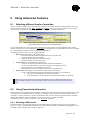
USING ADVANCED FEATURES ......................................................................................... 48
Selecting different levels of expertise ........................................................................................ 48
5.2
Page 2 / 81
TNO 2009 - SPOCS 6.0, User Guide
6.2
6.3
6.4
6.5
6.6
7
7.1
7.2
7.3
8
8.1
Using Power back-off models ................................................................................................... 48
6.2.1 Selecting a PBO model.................................................................................................... 48
6.2.2 Available PBO models, and its parameters ...................................................................... 49
6.2.3 Inspecting a PBO model .................................................................................................. 49
Using Receiver models (SPOCS/full only) ................................................................................ 50
6.3.1 Selecting an alternative Receiver Model .......................................................................... 50
6.3.2 Selecting tuneable receiver models .................................................................................. 52
6.3.3 Selecting a generic receiver model................................................................................... 53
6.3.4 Inspecting a receiver model (bitloading).......................................................................... 53
Adding user-definable models (SPOCS/full only) ...................................................................... 54
Calculating Equivalent Disturber Levels (SPOCS/full only)....................................................... 54
Running repetitive tasks via macros (SPOCS/full only).............................................................. 55
USING PLUG-INS (SPOCS/FULL ONLY) ........................................................................... 56
Loop Builder............................................................................................................................. 56
7.1.1 Why is this tool relevant? ................................................................................................ 56
7.1.2 Loop Builder Description ................................................................................................ 57
Loop Viewer............................................................................................................................. 62
Transmit Viewer ....................................................................................................................... 63
8.3
SUMMARY OF MENUS, BUTTONS AND FIELDS ............................................................ 65
Menu BAR ............................................................................................................................... 65
8.1.1 FILE Menu...................................................................................................................... 65
8.1.2 VIEW Menu (SPOCS/full only) ........................................................................................ 65
8.1.3 VIEW Menu (SPOCS/light only) ...................................................................................... 66
8.1.4 LIBRARY Menu............................................................................................................... 66
8.1.5 CONFIG Menu ............................................................................................................... 67
8.1.6 MACROS Menu (SPOCS/full only) .................................................................................. 68
8.1.7 TOOLS Menu (SPOCS/full only)...................................................................................... 68
8.1.8 WINDOW Menu.............................................................................................................. 69
8.1.9 HELP Menu .................................................................................................................... 69
Buttons ..................................................................................................................................... 69
8.2.1 On SPOCS/full only......................................................................................................... 69
8.2.2 On SPOCS/light only....................................................................................................... 70
Fields........................................................................................................................................ 70
9
9.1
9.2
9.3
9.4
NOMENCLATURE FOLLOWED FOR THE MODELS ..................................................... 72
Transmitter Model .................................................................................................................... 72
Receiver Model (SPOCS/full only) ........................................................................................... 72
Loop Model .............................................................................................................................. 73
PBO Model............................................................................................................................... 73
8.2
ANNEX A: TERMINOLOGY........................................................................................................... 74
ANNEX B: THE DIFFERENCE BETWEEN PSD TEMPLATES AND MASK............................. 77
ANNEX C: CHANGING DEFAULT SETTINGS............................................................................ 78
ANNEX D. REFERENCES ............................................................................................................... 81
Page 3 / 81
TNO 2009 - SPOCS 6.0, User Guide
List of Abbreviations
2B1Q
ADSL
BER
CAP
CMP
CO
CPE
DFE
DLC
DMT
DSLAM
EC
EL-FEXT
EPL
ETSI
FBL
FDD
FEXT
FSAN
GABL
HDSL
IMA
INP
ISDN
ISDN-BA
LT
LT-port
LTU
MDF
NEXT
NT
NT-port
NTU
OLR
PAM
PBO
POTS
PSD
PTM-TC
QAM
RBL
SDSL
SNR
SPOCS
SRA
TBL
TCM
TRA
UC
VDSL
xDSL
XTALK
2-Binary, 1-Quaternary (Use of 4-level PAM to carry two bits per pulse)
Asymmetric Digital Subscriber Line
Bit Error Rate
Carrier less Amplitude/Phase modulation
Cable Management Plan
Central Office
Customer Premise Equipment
Decision Feedback Equalizer
Digital Loop Carrier
Discrete Multi-Tone modulation
DSL Access Multiplexer
Echo Cancelled
Equal Level Far End Crosstalk
Estimated Power Loss
European Telecommunications Standards Institute
Fractional Bit Loading
Frequency Division Duplexing / Duplexed
Far-End Cross Talk
Full Service Access Networks
Gain Adjusted Bit Loading
High bit rate Digital Subscriber Line
Inverse Multiplexer for ATM
Impulse Noise Protection
Integrated Services Digital Network
ISDN Basic rate Access
Line Termination
Line Termination - port (commonly at central office side)
Line Termination Unit
Main Distribution Frame
Near-End Cross Talk
Network Termination
Network Termination - port (commonly at customer side)
Network Termination Unit
Online Reconfiguration
Pulse Amplitude Modulation
Power Back-Off
Plain Old Telephone Service
(Single-sided) Power Spectral Density
Packet Mode Transmission Trans-Convergence Layer
Quadrature Amplitude Modulation
Rounded Bit Loading
Symmetric single-pair high bit rate Digital Subscriber Line
Signal to Noise Ratio (ratio of powers)
Simulator for Performance Of Copper Systems
Seamless rate adaptation
Truncated Bit Loading
Trellis Coded Modulation
TRAnsmitter
“Ungerboeck Coded” (also known as trellis coded)
Very high bit rate Digital Subscriber Line
x-Digital Subscriber Line (term to encompass all DSL technologies)
Crosstalk
Page 4 / 81
TNO 2009 - SPOCS 6.0, User Guide
1 Disclaimer and copyrights
1.1
Copyrights of SPOCS and associated libraries
(c) 1996-2009 The Netherlands Organisation for Applied Scientific Research - TNO, Delft, the Netherlands.
All rights reserved.
No part of this publication may be reproduced and/or published by print, photo-print, microfilm or any other
means without the previous written consent of TNO.
1.2
Disclaimer
The origin of this software tool is branded as SPOCS© by TNO (Simulator for Performance of Copper Systems),
but is also distributed as 5D10 and 5C60 by Spirent. Although SPOCS was created with the utmost care, the end
user license rights are granted on a strict AS IS basis. TNO does not accept any liability for damage that the
owner or user of SPOCS might incur due to the use of this software. Reverse engineering of SPOCS and
associated libraries is strictly prohibited unless and to the extent explicitly permitted by relevant law.
The use of SPOCS is subject to specific end user license conditions as integrated in the software, as amended
from time to time.
1.3
Third party rights
SPOCS has been compiled using the MATLAB compiler and associated MCR-libraries. The MCR runtime
libraries are licensed components of MATLAB, (c) 1984-2007, The Mathworks, Inc.
The installer has been compiled using an open source scripting language NSIS. It can be obtained via
nsis.sourceforge.net
1.4
Support
Support, sales and licenses inquiries on SPOCS can be obtained via www.spocs.nl
Page 5 / 81
TNO 2009 - SPOCS 6.0, User Guide
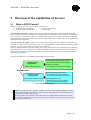
2 Overview of the capabilities of the tool
2.1
What is SPOCS about?
SPOCS is equipped to assist you in two kinds of applications:
• Predicting DSL performance
--> Performance simulator
• Creating custom noise profiles
--> Noise profiler
Predicting DSL performance. SPOCS can be used to predict the performance of DSL modems under noisy
stress conditions (loops and crosstalk from other DSL modems). Performance can be evaluated as maximum bit
rate, as margin or as reach, both as plot or in a tabular format. Plots of the spectral results (PSD’s of noise and
signals being received by the modems under test) can be generated as well. All these plots can be copied via the
clipboard to other applications.
Creating custom noise profiles. SPOCS can be used to define complicated noise profiles to control the noise
generators in a DSL test setup. This allows users to tests the performance of DSL modems in a lab environment
(testloop + noise generator) under user-defined noise conditions.
Define in SPOCS an arbitrary scenario of loops and systems, calculate the noise spectrum that will result from
that system mix on a wire line, and save it to file The resulting profile (in a tabular ASCII format) can serve as
input for noise generators that allow the generation of custom-specified noise (such as the Spirent DLS5204
series of noise generators).
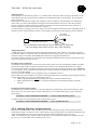
These functionalities are to serve different applications, as shown below:
Predicting DSL
performance
(Reach | Bitrate | Margin)
Spectral Management (SpM) studies
(for allowing new DSL technologies)
Deployment studies
(for deploying new DSL technologies)
Software tool
Creating custom
noise profiles
(Defining Noise Environments)
Measuring/testing performance
under all kinds of noise conditions
(for selecting new DSL technologies)
Measuring performance
under all kinds of noise conditions
(for improving new DSL designs)
Figure 1: SPOCS Functionality.
NOTE: This software tool is available in different versions. When branded as SPOCS or 5D10, it
can do both performance predictions, but the 5C60 has disabled prediction functionalities (noise
profiles only, tailored to DSL testing)
The GUI (graphic user interface) of the light version is a slightly different from the full version.
For reasons of simplicity both versions are described in the same manual, showing the GUI of the
full versions in most cases.
Page 6 / 81
TNO 2009 - SPOCS 6.0, User Guide
2.2
Using SPOCS as DSL Performance simulator
A primary functionality of SPOCS is the ability to predict the performance of a DSL system under various
operational stress conditions. This stress includes the impairment of a large number of different xDSL disturbing
neighbouring systems at arbitrary locations, and the loss and crosstalk coupling of different cable types at
arbitrary lengths.
Performance is a generic term that can be represented in different ways. SPOCS can represent this performance
as (a) maximum bit rate, as (b) noise (or signal) margin and (c) as reach. Bit rates and margins are usually
presented as a function of the loop length, but other parameters may also be used for that (e.g. as a function of
the number of disturbers).
SPOCS can evaluate bit rates and margin in a direct way, and evaluates reach in an iterative way. They can all be
evaluated for a range of operational stress conditions (signal loss in loops, and noise due to other disturbers and
crosstalk coupling), and for a range of modems (like ISDN, SDSL, HDSL, ADSL, ADSL2plus, VDSL, VDSL2,
etc). SPOCS can present this predicted performance in both a graphic way (plot) and a tabular way (in a
textbox).
SPOCS can also provide the end-user with intermediate calculation results, such as for instance the power
spectral density (PSD as function of the frequency) of signals (transmitted, received, etc) and noises (total
crosstalk, NEXT-only, FEXT-only, etc).
Max bitrate @ specified margin
(all for various loop lengths)
maximum
BIT RATE
performance
REACH
Reach @ fixed bitrate
(at 6 dB noise margin)
MARGIN
Noise margin @ fixed bitrate
Signal margin @ fixed bitrate
(all for various loop lengths)
Figure 2: Different ways to express the performance of a system.
2.2.1 Example 2: Spectral Management (SpM) Studies
Once a technology is identified as attractive, it still may have a negative impact on the integrity of deployed
services. A well-known example is the deployment of VDSL2 from a street cabinet, while ADSL2plus systems
are deployed in the same cable from the local exchange. Without proper measures (shaping VDSL2 transmit
power), the impact on ADSL2plus will be very negative.
With SPOCS you can perform impact analyses, and quantify how much impact a specific amount of PSDshaping will have on both ADSL2plus as well on VDSL2 itself. If zero impact on ADSL2plus means a high
associated bit rate reduction of VDSL2, a compromise may be considered.
Page 7 / 81
TNO 2009 - SPOCS 6.0, User Guide
2.2.2 Example 1: DSL deployment Studies
The DSL noise environment is country-specific. Some systems are not allowed (or not deployed) in some
countries, while the number of wire pairs per cable and the characteristics of these cables are country-specific.
When new and promising xDSL technologies come available, it is not obvious how it will perform in a particular
noise environment. However, this is essential information for making strategic decisions on deploying such
systems.
With SPOCS you can make performance predictions that are tailored to the noise environments of your
preference. Not only for strategic decisions but also to develop deployment guidelines, to identify what bit rate
be promised at what quality (margin) to a certain loop length.
2.3
Using SPOCS to create custom noise profiles for DSL testing
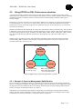
Another functionality of SPOCS is the ability to evaluate the PSD (power spectral density) of crosstalk noise, as
it will be observed by the receiver of a (victim) modem. This is an intermediate result of a full performance
prediction, but a target result for performance testing in the lab.
The profiler functionality of SPOCS enables the user to export this PSD as a noise profile and to download it
into a noise generator. In other words, SPOCS can specify the Noise Profile for a noise generator as part of a test
setup to verify, for instance, modem performance.
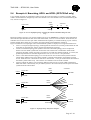
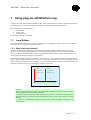
Figure 3 shows a simplified scenario of a DSL setup with Near-End Cross Talk (NEXT) and Far-End Cross Talk
(FEXT) contributions. This oversimplified example is restricted to single disturbers at each side of the line.
When more disturbers are involved, and/or located at different positions, SPOCS handles their combination.
DSL under test
DSL under test
LT transmitter DS
NT receiver DS.
LT receiver US
NT transmitter US
NEXT
NEXT
Downstream
disturber
FEXT
systems
Upstream
disturber
systems
Figure 3: A simplified scenario for a test setup, that can be evaluated by SPOCS.
2.3.1 Example 1: DSL performance testing
If you are a vendor of xDSL technology, designing new products, you can optimize the modem design by testing
its behaviour. Your modem will be used in a wide range of very different operational conditions that are
sometimes very different from the few “standard” stress conditions defined by bodies like ETSI and ITU.
Similar to the previous example, SPOCS can generate all kinds of noise profiles for testing purposes, which are
valuable in improving products. For example, chipset manufacturers or academic users can apply their new
algorithms (for coding or spectral usage) and evaluate how much performance gain it will really bring.
2.3.2 Example 2: Product selection
Similar xDSL solutions from different vendors perform differently. They all may pass standardized tests, but
these tests are usually still under development when new technology becomes available. In addition, standard
stress conditions are usually very different from operational noise environments.
With SPOCS you can make product assessments that are tailored to the noise environments of your preference.
SPOCS can predict a noise environment, and create a noise profile of the spectra that can be observed by a
modem under study. When such a noise profile is fed to a noise generator (that supports the creation of userdefinable noise), you can test in your lab how a particular modem implementation will really perform under
noisy stress conditions.
Page 8 / 81
TNO 2009 - SPOCS 6.0, User Guide
3 Quick Start Examples
This quick start provides you with two examples for using SPOCS. One dedicated to performance testing
(profiler functionality) and another to performance simulations (predictor functionality).
3.1
Loading a first example scenario
SPOCS comes with several example scenarios. These can be found on:
<InstallDir>\Examples\Examples_manual.
Once SPOCS is started, you can load your first example scenario via the menu:
[FILE | LOAD] → select <InstallDir>\Examples\Examples_manual\quickstart_1.ssf
To make that directory the current directory, for easy loading other scenarios in the same directory, you can do
that via the menu:
[FILE | FOLLOW DIRECTORY]
The scenario used for a simulation will be called henceforth a “Simulation Scenario”.
3.2
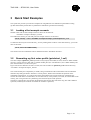
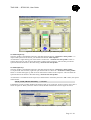
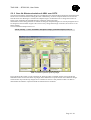
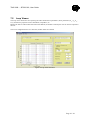
Generating my first noise profile (quickstart_1.ssf)
This first example (quickstart_1.ssf) represents a noisy loop (0.5mm cable) of 3 km, where an ADSL modempair (the “victim”) shares a cable with 15 similar modem pairs (the “self disturbers”) and 3 SDSL modem pairs
(the “alien disturbers”) on other wire pairs.
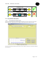
Figure 4 shows the definition of such a scenario, that can be loaded via quickstart_1.ssf from the directory
<InstallDir>\Examples\Examples_manual.
The victim modem pair is impaired by crosstalk, being a cumulation of the contributions from all individual
disturbers. By hitting the button “Generate LT noise profile”, SPOCS will calculate the spectrum of the
cumulated crosstalk noise, as it will be observed by the modem at the LT side of the loop (commonly the
location of a DSLAM in a central office). It saves the result (a “noise profile”) into a file, in a format that can be
used by your noise generator for synthesizing noise with exactly the same spectrum.
The button “Generate NT noise profile” facilitates the same for the other side of the loop, but with a different
spectrum (commonly the location of a CPE at the customer’s premises).
Page 9 / 81
TNO 2009 - SPOCS 6.0, User Guide
Figure 4: Scenario definition for my first noise profile.
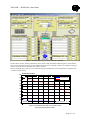
For SPOCS/full only:
SPOCS can show you the generated spectra in advance, but this is disabled by default. Enable this first via the
“View” menu:
[VIEW | Show Spectra] → select it if the check marker is absent
Hit the “RUN” button, and the plots in figure 5 and 6 will be shown.
For SPOCS/light only:
SPOCS can show you the generated spectra in advance. Hit the “Show Spectra” button, and the plots in figure 5
and 6 will be shown.
Page 10 / 81
TNO 2009 - SPOCS 6.0, User Guide
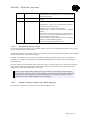
LT spectra: Upstream signal, received noise
-20
PSD [dBm/Hz]
[1]
-40
[1] Transmitted Signal, @100 ohm
[2] Receiv ed Signal, @100 ohm
[3] Receiv ed Noise, @100 ohm
-60
-80
[3]
-100
[2]
-120
-140
-160
-180
-200
[SPOCS]
-220
Freq [Hz]
0
500k
1M
1.5M
2M
2.5M
Figure 5: Spectra at the LT side of the loop, as specified in figure 4.
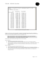
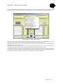
NT spectra: Downstream signal, received noise
-20
PSD [dBm/Hz]
-40
[1] Transmitted Signal, @100 ohm
[1]
[2] Receiv ed Signal, @100 ohm
[3] Receiv ed Noise, @100 ohm
-60
[2]
-80
-100
[3]
-120
-140
-160
-180
-200
[SPOCS]
-220
0
Freq [Hz]
500k
1M
1.5M
2M
2.5M
Figure 6: Spectra at the LT side of the loop, as specified in figure 4.
3.3
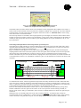
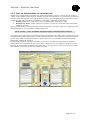
Generating my first performance prediction (SPOCS/full only)
This second example (quickstart_2.ssf) represents again a noisy loop (0.5mm cable), where an ADSL modempair (the “victim”) shares a cable with 15 similar modem pairs (the “self disturbers”) and 3 SDSL modem pairs
(the “alien disturbers”) on other wire pairs. Figure 7 shows the definition of such a scenario, which can be loaded
via quickstart_2.ssf from the directory <InstallDir>\Examples\Examples_manual. It is very similar to the one in
quickstart_1.ssf, but with the difference that it now sweeps the loop length in steps of 250 meter from 500m up
to 5000m.
To change this sweep, redefine the “sweep parameter k1” as [<start value> : <step value> : <stop value> ] as
explained in more detail on section 4.2.5. If you prefer feet over meter, see section 4.2.6 for further details.
Page 11 / 81
TNO 2009 - SPOCS 6.0, User Guide
Figure 7 : Scenario definition for my first performance simulation.
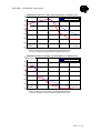
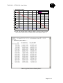
Hit the “RUN” button, and the performance plot in figure 8 and performance table in figure 9 will be shown.
They represent the bitrate that a (victim) modem pair under test is expected to achieve (at 6 dB noise margin)
when it is impaired by the disturbers of the above scenario.
If the loop length equals 3km, you can read from the plot (and table) that it will be 862 kb/s in upstream and
7.02Mb/s in downstream.
10M
Performance Plot
[b/s]
9M
[1] DataRate Up
[2]
[2] DataRate Dn
8M
7M
6M
5M
4M
3M
2M
1M
[1]
[SPOCS]
0
500
1k
Sweep Parameter
1.5k
2k
2.5k
3k
3.5k
4k
4.5k
k1 -->
5k
Figure 8: Predicted data Rate (Mb/s) as a function of the
loop length [m] (Performance Plot).
Page 12 / 81
TNO 2009 - SPOCS 6.0, User Guide
Figure 9: Output Text File (Performance Table).
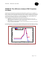
SPOCS can also show you the spectra that are evaluated as intermediate result. This option is disabled by
default, since it slows-down the performance evaluations significantly. Enable this first via the “View” menu,
where you can also modify what kind of spectra you would like to see.
[VIEW | Select Spectra] → Here you can choose the signals you want to plot and analyze.
[VIEW | Show Spectra] → select it if the check marker is absent
Hit the “RUN” button, and the plots in figure 10 and 11 will be shown.
Figure 10 shows:
• The upstream signal transmitted from the NT side
• The received upstream signal (LT-side) being attenuated by the loop and modem impedances
• The received noise spectra (LT-side) for each length of the loop, which is a combination of FEXT from
upstream disturbers, NEXT from downstream disturbers and other disturbers (Line shared noise,
background noise).
Figure 11 shows:
• The downstream signal transmitted from the LT side.
• The received downstream signal (NT-side) being attenuated by the loop and modem impedances
• The received noise spectra (NT-side) for each length of the loop, which is a combination of FEXT from
downstream disturbers, NEXT from upstream disturber and other disturbers (Line shared noise,
background noise).
Page 13 / 81
TNO 2009 - SPOCS 6.0, User Guide
LT spectra: Upstream signal, received noise
-20
PSD [dBm/Hz]
[1]
-40
[1] Transmitted Signal, @100 ohm
[2] Receiv ed Signal, @100 ohm
[3] Receiv ed Noise, @100 ohm
-60
-80
[2]
[2]
[2]
[2]
[2]
[2]
[2]
[2]
[2]
[2]
[2]
[2]
[2]
[2]
[2]
[2]
[2]
[2]
[2]
-100
-120
-140
[3]
-160
-180
-200
[SPOCS]
-220
Freq [Hz]
0
500k
1M
1.5M
2M
2.5M
Figure 10 : Upstream signal transmitted at the other side of the line, received upstream
signal (LT-side) and received noise at LT-side.
NT spectra: Downstream signal, received noise
-20
PSD [dBm/Hz]
-40
[1]
-60
-80
[1] Transmitted Signal, @100 ohm
[2] Receiv ed Signal, @100 ohm
[2]
[2]
[2]
[2]
[2]
[2]
[2]
[2]
[2]
[2]
[2]
[2]
[2]
[2]
[2]
[2]
[2]
[2]
[2]
[3] Receiv ed Noise, @100 ohm
[3]
[3]
[3]
[3]
[3]
[3]
[3]
[3]
[3]
[3]
[3]
[3]
[3]
[3]
[3]
[3]
[3]
[3]
-100
-120
-140
-160
-180
-200
[SPOCS]
-220
0
Freq [Hz]
500k
1M
1.5M
2M
2.5M
Figure 11 : Received downstream signal (NT-side), received noise at NT-side and
downstream signal transmitted at the other side of the line.
Page 14 / 81
TNO 2009 - SPOCS 6.0, User Guide
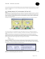
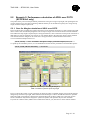
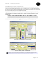
4 Defining and running scenarios
4.1
Overview of the GUI
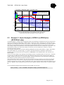
The main panel of the Graphic User Interface (GUI) of SPOCS is shown in figure 12. From here you can define
and run all your scenarios of interest:
• Defining the stress environment (loops, crosstalk, disturbers, frequency range).
• Defining a sweep, for instance to calculate performance as a function of the loop length.
• Defining the modem pair under study (victims).
For performance predictions you have to define them all, but if only a noise profile is to be defined you can leave
the system under study undefined (the E-blocks are simplified in SPOCS/light).
This section discusses how to define an arbitrary scenario and how to export the associated noise or to run a
performance simulation.
Terminology
A loop is a connection between two modems via a single wire pair. A loop has two sides or ports (LT and NT)
and therefore also two transmission directions (downstream and upstream):
• LT = Line Termination, a neutral name of the loop side that is closest to the core network. In many
cases, it is located at the central office (CO), where the modem is part of the DSLAM, but it could also
be in a street cabinet, in a distribution point or in a repeater at the customer side.
The LT is always on the left” side in the GUI of SPOCS.
• NT = Network Termination, a neutral name of the loop side that is opposite to the LT side. In many
cases, it is located at the customers premises (where the modem is called CPE - customers premises
equipment), but it could also be in a repeater at the central office side.
The customer is always right in the GUI of SPOCS.
• Downstream = transmission from LT to NT
• Upstream = transmission from NT to LT
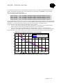
Figure 12: Overview of the GUI.
Page 15 / 81
TNO 2009 - SPOCS 6.0, User Guide
Stress environment
Loops and crosstalk
Section
4.2.1
4.2.2
4.2.3
Disturbers
Frequency range
Sweeps+Constants
DSL system under study
Victim modem
4.2.4
4.2.5
4.5.1
A
→
B1
B2
C
D
→
→
→
→
E1
E2
→
→
(for both SPOCS/full and SPOCS/light)
Loop model, cable and length between these modems
and crosstalk coupling parameters
Crosstalk disturbers for LT and NT
Other disturbers for LT and NT
Frequency range and count
Sweep parameter k1, and constants k2 and k3
(only for SPOCS/full)
LT Side, of modem link under study
NT Side, of modem link under study
Figure 13: Overview of the main blocks in the GUI of SPOCS.
4.2
Defining a stress environment
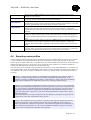
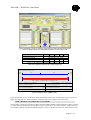
4.2.1 Defining a loop topology
Loops
The definition of a loop topology starts with selecting a suitable cable model. You can select a cable model from
a list with many predefined models, including predefined models for composite cables being defined in various
DSL standards (ETSI, ITU, DSLF). In the example below, we have selected cable model “KPN_L1”, which
represents a cable with 0.5 mm wire pairs (commonly used in the Netherlands)
Sections
A loop can be subdivided in multiple sections, to enable loop topologies where modems are deployed from
different locations. A two section topology can be adequate to represent a central office (from where ADSL is
deployed), a street cabinet (from where VDSL2 is deployed) and a few customer locations that are all
approximated as “co-located”.
Figure 14 illustrates how to subdivide a single loop of 3km into multiple sections. The more (comma separated)
numbers you add to the field where the loop length is defined, the more sections will occur. If you change the
number of sections, the GUI will immediate respond to that by a symbolic drawing above the length field.
In SPOCS, all cable sections must have equal properties per unit length, so a cascade of a 0.5 mm cable with a
0.8mm cable is not possible from the GUI. This requires the use of a composite loop model, as explained in
section 7.1.
Figure 14: Defining loops of 3km length, but with a different number of sections.
Page 16 / 81
TNO 2009 - SPOCS 6.0, User Guide
Nodes
The end of each section is demarcated by a unique sequential node number, so a loop has two or more nodes.
This enables you to define the location of modems in the loop topology. Figure 15 illustrates how to specify the
node of the modem at the NT-side of the loop (customer premises). If you change the node number of a victim
modem, the GUI will immediate respond to that by changing the node color in the symbolic drawing above the
length field.
• Red is used for nodes connected to a victim node
• Green is used for all other nodes
• Black is used for the “zero” node, to show that it is not connected.
• Blue is used when a node number is out of range (and no part of the topology)
Node numbers are to be sequential and to be specified by a single character, so 0,1,2,3,..8,9,A,B,C,D,..Y,Z. This
means a maximum of 35 nodes, or 34 sections. A modem link uses two nodes, and by convention the node
number at the NT side of the link (left, central office) is always lower than at the LT side (right, customer
premises).
Figure 15: Connecting the NT modem to different nodes of a loop.
Sweeping section lengths
Many performance calculations are presented as a function of the loop length, meaning that such a length
“sweeps” between a minimum and maximum values in predefined steps. A section length can be made flexible
by defining its length as an expression that involves the “sweep parameter” k1. This is a fundamental concept
within SPOCS, which is explained in more detail in section 4.2.5. When the sweep parameter k1 is used to
define a section length, SPOCS will analyze the scenario for all the values being allocated to k1.
Figure 16 illustrates how to define this. On the left picture it is used only once in one section, but on the right
picture it is used in two sections at the same time by means of an expression. This gives you virtually unlimited
means to specify topologies with an arbitrary dependency of the sweep parameter “k1”. In both cases, the sweep
parameter k1 is specified as a list of values, starting in this example with k1=500, ending with k1=5000 and in
steps of 250.
Mark that when k1 is used in a section length the total loop length is not a fixed value anymore. The GUI
responds to that by showing the shortest and the longest length of the loop that can be achieved with the current
definitions. It adapts immediately to changes in the definitions of section lengths or sweep range.
Figure 16: The length of sections in a loop can be made flexible by replacing a constant by
the loop parameter k1, to sweep the loop length from short to long.
Page 17 / 81
TNO 2009 - SPOCS 6.0, User Guide
Inspecting section lengths
The symbolic drawing of the sections above the “length field” is not to scale. For your convenience, SPOCS can
make a graphic representation of the loop topology that you have defined. Push the <Show> button, to draw the
topology on scale.
Figure 17 shows it for the fixed-length examples in figure14. When the length of one or more sections is
specified by means of the sweep parameter k1, the highest value for the sweep parameter k1 is used to draw the
topology. The red line (marked with “V”) illustrates what loop section(s) are being used by the (victim) modempair under test; in this example between node “1” and “2”.
Loop range: [1000, 500, 1500] →
(3000 m)
(Only the maximum values are drawn below)
[SPOCS]
1000
500
DSLAM
[LT]
[1]
[2]
1500
[3]
[4]
<downstream> →
← <upstream>
CPE
[NT]
V:
LOOP:
V = Victim,
D = Disturber,
[KPN_L1]
= undergrou nd cable L1 ( 50×4×0.5mm), 0.5km
[1]..[4] = NodeNumber
NEXT = -50 dB[1Mhz],
V.t = --V.r = ---
EL-FEXT = -45 dB[1Mhz,1km]
V.t = --V.r = ---
Figure 17: Graphic representation of the topology being created.
More examples of section lengths
It may be clear that SPOCS allows for a lot of flexibility in defining the section lengths of a loop topology. The
means for specifying section lengths are virtually unlimited. It allows numbers, the sweep parameter k1,
constants k2 and k3, and all kinds of expressions from these. The examples below give a view on the different
possibilities.
Case A:
Case B:
Case C:
[k1]
[k1*2 + 400]
[k1*2 + k2*k3]
à
à
à
Case D:
[k2+3*k3]
à
Case E:
Case F:
Case G:
Case H:
[2000, 1500]
[500, 500, 500, 250, 250]
[100, 100 + 250*2, 250*4, 250]
[500, k1]
à
à
à
à
one section, swept via k1
one section, swept via an expression with k1.
one section, swept via an expression with k1 and
two constants k2,k3
one section of constant length, via an expression
with k2 and k3
Two sections of constant lengths
Five sections of constant lengths
Four sections of constant lengths
Two sections, the second one is swept
Case I:
[100, k2, k3, k1]
à
Four sections, all constant except for the last one
In principle you can even use more advance expression, including all kinds of mathematical functions like
min(k1,5000), max(100,k1), abs(k1), exp(k1) and sin(k1). However most of them may go beyond what is needed
for defining realistic scenarios. It uses the same syntax as within the third-party tool Matlab (from the
Mathworks)
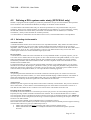
4.2.2 Defining crosstalk coupling in the loop
The default values for NEXT and EL-FEXT coupling in the cable are visible via the GUI, as shown in figure 18.
The NEXT value represents the (normalized) near end crosstalk coupling at 1MHz, and the EL-FEXT value
represents the (normalized) equal-level far end crosstalk of 1 km cable at 1 MHz. The values used in figure 18
are pragmatic values that have been used in many DSL standards.
Page 18 / 81
TNO 2009 - SPOCS 6.0, User Guide
Figure 18: The crosstalk coupling values for NEXT and equal level
FEXT can be modified. The values hold for all loop sections.
The default values for NEXT and EL-FEXT can be modified via the configuration file of SPOCS (see annex C).
These values are also tuneable via the GUI, but this is disabled on default. If it is grayed-out, and you would like
to change them, you must switch the level of expertise from “basic mode” to “advanced mode” via the config
menu. See section 6.1 for further details.
Since all loop sections are assumed to have equal properties per unit length, the values for NEXT and EL-FEXT
hold for all sections. So NEXT is always to be specified by a single value, and the same applies for EL-FEXT. If
needed you may specify that value by a number, by the sweep parameter k1, by the constants k2 or k3, or even
by an expression.
Some background information on the interpretation of crosstalk power
The models for crosstalk coupling are used to evaluate the crosstalk power in the wire pair under study, which
originates from all disturbers in other wire pairs. The meaning of the crosstalk power is not obvious, and some
physical background is needed to understand why.
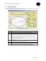
Figure 19 illustrates what happens in a real cable. Each loop has multiple wire pairs, and the electromagnetic
coupling between these wires causes that systems in other wire-pairs induce crosstalk noise in the wire pair that
interconnects the victim modem pair. In practice, however, there is a significant spread in coupling values
between individual wire pairs. Even when all these coupling factors are exactly known, the overall crosstalk will
not be deterministic if there is no information to what wire pairs a set of disturbers are connected. So how to deal
with that?
(Local Exchange)
modem
under
downstream
upstream
LT-side
(Customer Premises)
NT-side
study
modem
under
study
mixture of
mixture of
xDSL
disturbers
xDSL
disturbers
cable
wire pair
Figure 19: Crosstalk Coupling in the Loop.
To understand the answer, assume a hypothetical experiment with many modems and a cable. When that cable
with N wire pairs is filled-up completely with similar disturbers, the resulting crosstalk power in each wire-pair
(from N-1 disturbers connected to the other wire-pairs) is maximal and therefore unambiguous. This upper limit
is the saturated crosstalk power for that type of disturber, for that particular wire-pair.
However if the number M of disturbers is lower (M<N-1), this crosstalk power will commonly change when
another combination of M wire-pairs will be chosen. So an exact expression for the resulting crosstalk, as
function of the number and type of disturbers, does not exist if it remains unknown to which wire-pairs they are
connected.
What does exist are crosstalk powers that occur with a certain probability. To illustrate that, consider an
experiment that connects 30 disturbers to a cable with 100 wire pairs in 100.000 different ways. If the resulting
noise is observed in one particular wire-pair, it is most likely that you will also observe 100.000 different
Page 19 / 81
TNO 2009 - SPOCS 6.0, User Guide
crosstalk noise powers. The result of such a “probability experiment” is therefore not a single power, but a
(wide) range of powers with a certain probability distribution.
Within this range, a certain crosstalk noise power can be found that is not exceeded in X% of the cases. That
power level is named a probability limit for a particular wire pair, and the crosstalk models in SPOCS are to
predict how such a limit behaves as a function of number and type of disturbers.
The crosstalk models in SPOCS are to predict the noise levels associated with the 99% worst case limits, because
that criteria is commonly used. The modeling follows the FSAN sum to cumulate all crosstalk (see ETSI SpM-2
[1]). As a result, you are to provide values for the normalized NEXT and EL-FEXT of a cable as a whole, and
not the NEXT and EL-FEXT between individual wire pairs.
When SPOCS evaluates the performance under a noise power that equals the 99% probability limit, you should
realize that in “most cases” the actual performance will be better then predicted! The use of 100% worst case
limits is commonly avoided, to prevent for over-pessimistic analyses.
NOTE: The noise levels in xDSL product standards, that are specified for testing purposes, are all
defined by using that "99% worst-case" rationale. It means more or less "If the modem can survive
from this noise level, it will work in almost all cases of a scenario".
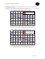
4.2.3 Selecting disturbers
A disturber is a source that impairs the performance of the (victim) modem under study. Like victims, disturbers
come also in pairs.
Crosstalk disturbers
These disturbers are representing modems in other wire pair, that couple into the wire pair of the victim modem.
On default, when you select a disturber on one side, SPOCS will automatically select the associated one at the
other side. The naming convention uses the following prefixes:
• TPL: denotes that a model represents a template PSD of an individual modem
• MIX: denotes that a model represents the equivalent of a mix of disturbers (as defined in standards)
Their contribution to the overall impairment depends on the NEXT and EL-FEXT setting, as well as the length
and insertion loss of the coupled sections
Direct disturbers
These disturbers are representing modems using the same wire pair as the victim modem under test, but in
another frequency band. It is typically used to add “line shared” noise (like from ISDN systems) or
“background” noise (from unidentified sources). On default, when you select a disturber on one side, SPOCS
will automatically select the associated one at the other side.
Its contribution to the overall impairment is independent from the NEXT and EL-FEXT setting.
Node selection
Disturbers inject their signal in the loop from a location that is named by a node number. A node value ‘0’ means
that the disturber is inactive. They can be co-located with the two victim modems or be at different locations like
in street cabinets or distributed along the line. More details can be found in section 4.2.1.
Note that the node number at the LT side has to be lower then the node number on the NT side.
Increasing disturber count or scale
Increasing the count for one disturber pair is exactly the same as defining an equal amount of identical disturber
links. It is implemented by increasing the level of the disturber in a special way. Leave the mouse pointer a few
seconds above a field for specifying how much dB this increase will be.
Expert users may consider specifying this increase directly in dB’s. In such a case, hit the “count” button so that
its label changes to “scale”. Now you can specify yourself how much dB is required to represent multiple
disturbers.
Page 20 / 81
TNO 2009 - SPOCS 6.0, User Guide
Adding Branches
Most topologies are branched in practice. It is common that a distribution cable, leaving a central office (“LT”)
with 900 wire pairs, fan out from a street cabinet into 9 independent cables of 100 wirepairs. This is depicted
below in figure 20.
Branching is the mechanism to define such topologies. It has an impact on the performance of a modem pair
under study, since most of the disturbers starting from the central office do not arrive at the same customer
location. Topologies without branching are often too pessimistic about the performance being predicted. A
detailed example of such a study is discussed in section 5.4.
To add a branch to a topology, hit the “B” button to specify the length of the branch for each individual group of
disturbers. Hit the “Show Topology” button to see a graphic representation of the topology you have defined.
nine cables
100 wire pairs each
NT
LT
single cable, 900 wire pairs
Figure 20 Distribution cables usually fan out from street cabinets or underground
splices into multiple cables with less wire pairs. This is called “branching”.
Adding PBO models
A PBO model forces some amount of power back-off of the transmit power, before it is injected into the loop.
For instance, ADSL is required to reduce its downstream when the loop is short, to prevent that the modem at the
customer side gets overloaded. Hit the PBO button and select an appropriated model for it.
The amount of power reduction is not fixed but may depend from different factors, like the insertion loss of the
loop or the signal power being received.
Extending the list of disturbers
On default, the list of disturbers is restricted to prevent that you get lost in an overwhelming number of models.
Especially the large number of VDSL2 models has been reduced. This is because SPOCS starts in a “Basic”
level of expertise, which is intended only during a learning period. We recommend switching to the “Advanced”
level of expertise via the config menu (and do not give in to the temptation of selecting the “Expert” mode!). See
section 6.1 for further details.
You can overrule this default via the configuration file, as explained in annex C.
More models will come available if you switch to the Expert mode and it will disable protection against selecting
invalid models. However it gives you additionally access to:
• Models representing PSD masks specifying peak values instead of nominal values
• Models intended for the “other side” to study the transmission of downstream signal in upstream
direction.
Disabling the autocompletion modes
On default, when you select a disturber on one side, SPOCS will automatically select the associated one at the
other side. In case your study requires another combination, you can disable this behavior via the following
menu setting:
[CONFIG | AUTO COMPLETION MODES > → deselect “Keep disturbers paired”
To enable it only once (for all disturber and victim modems), select:
[CONFIG | AUTO COMPLETION MODES > → select “Synchronize once”
4.2.4 Defining frequency range and count
Impairment and performance is only calculated with the selected frequency range, at the specified resolution.
The frequency range is set from 0 to Fmax. This frequency range should at least cover the full transmission band
of the victim modem (plus a bit extra), otherwise it cannot calculate performance in a correct way.
ADSL uses frequencies up to at least 1.1MHz; ADSL2plus up to 2.2 MHz, and VDSL2 uses frequencies in the
up to 8.5,12, 17 and 30 MHz. Fmin is always forced to zero.
Page 21 / 81
TNO 2009 - SPOCS 6.0, User Guide
Count provides the linear resolution that SPOCS will use when evaluating the system under study, i.e. if Fmin=0
and Fmax=1200 KHz, then a count value of 5000 indicates that the resolution is approximately equal to (12000)/5000 = 0.24 KHz.
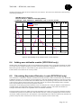
4.2.5 Defining sweeps (“k1”) and constants (“k2” and “k3”)
Sweeps
The performance of a system under specific stress conditions is a single value: margin or bitrate. It is, however,
more convenient to calculate multiple performance values for a range of stress conditions and to present it as a
plot. For instance the attainable bitrates as a function of the loop length, or the noise margins as function of the
number of disturbers. To facilitate that, SPOCS has a powerful feature on board to do that in a highly flexible
manner: the sweep parameter k1.
Examples of its use for a range of loop lengths have been discussed in section 4.2.1 and shown in figure 21.
Figure 21: The length of sections in a loop can be made flexible by replacing a constant by
the loop parameter k1, to sweep the loop length from short to long.
This sweep parameter k1 is a fundamental concept within SPOCS, and gives you inlimited possibilities to
evaluate the performance as a function of “something”. Its definition is essentially a comma-separated list of
values.
As soon as the parameter k1 is used anywhere on the front page of the GUI, the simulator evaluates the
performance for each value within that list. It does not matter where k1 is used: it can be to define the loop
length, a single section of a loop, the number of disturbers, crosstalk coupling, etc. You can use it on multiple
places at the same time, both as a single value or as an expression. For instance:
k1
k1+275
3*(812-k1)+26*k2
The syntax of defining the list of values for k1 is similar to the syntax being used by the third-party program
“Matlab” for defining a row-matrix. The format of this parameter is [Min:step:Max] or [val1, val2, val3] or a
mix of them, i.e. [100:100:1500] which means that the first value is 100, it will continue in steps of 100 and the
last value will be 1500. Other examples are summarized below:
Format
[Min: Max]
Example
[100:400]
[Min:step:Max]
[val1, val2, val3]
[val1]
[val1, min:step:max]
[100:100:400]
[100,400,1000]
[500]
[200, 400:50:700]
Output
k1 contains values from 100 to 400 in steps of
one unit.
k1 contains 100,200,300,400 values
k1 contains values 100,400 and 1000.
k1 contains only one value, 500.
k1 contains 200, 400, 450,500, 550, 600, 650
and 700.
When k1 is not used anywhere in the scenario or has only one single value, then a single result will occur (single
performance value and/or single PSD, at LT and NT side).
Page 22 / 81
TNO 2009 - SPOCS 6.0, User Guide
Constants
The fixed parameters k2 and k3 are single values (constants, no list of values) that you can use anywhere in the
definition of the scenario. This can keep the specification readable, especially when k2 (or k3) is used at
different places at the same time. A typical application occurs for scenarios with sub-loops:
• Example 1: We can set up k1= k3 + [0:50:k3], k2=4000, k3=1500 and Length = [k2/2, k1-k3] leading
to an analysis where node 2 is fixed (2000 m away from the first node) and the distance between the
second node (CAB) and the third one (CPE) is swept from 0 to 1500 m.
• Example 2: The sweep parameter k1 might be also set to k3 + [k3:-50:0], k2=4000, k3=1500 and
Length = [k2/2, k1-k3] leading to identical results.
You can use one constant in the other parameters if you account for the order of evaluation. SPOCS evaluates k3
first, then k2 (and may use the result of k3), and finally k1 (and may use the results of k3 and k2).
The use of k2 and k3 is disabled when working in the basic mode. You can increase the level of
expertise via the CONFIG menu item. See section 6.1 for further details.
4.2.6 Using metric or imperial units
SPOCS allows changing the units between metric an imperial units according to a user-definable choice.
Units in displayed results. All calculations are done in metric units, whatever the unit settings are, but results can
be displayed in imperial units as well. The available units in SPOCS are 'meter', 'km', 'inch', 'feet', 'yard', 'kft' and
'mile'. On default, results are presented in meter but this default can be changed via a configuration file. See
annex C for further details. You can also change it from the GUI via the menu:
[CONFIG | UNITS (for displaying values only) > → select unit of interest
Units in input fields. All fields require metric units, independently from what units are selected for displaying
results. To enable a convenient way to specify loop length in units like yards and kft, various conversion
constants are predefined. Entering the expression “3*kft” reads like imperial units and still produce a length in
meter. These kinds of expressions can be used in any field on the GUI front panel, including the fields for loop
length, sweep parameter k1, constants k2 and k2, etc.
Figure 22 summarizes the predefined conversion constants, and figure 23 provides a few examples on how to use
them. There names are case sensitive
Conversion constant
inch
feet
yard
kft
mile
Remark
(1 inch = 0.0254 m)
(1 feet = 12 inch = 0.3048 m)
(1 yard = 3 feet = 0.9144 m)
(1 kft = 1000 feet = 304.8 m)
(1 mile = 1760 yard = 5280 feet = 1609.3 m)
Figure 22: Predefine conversion constants to convert length into meters.
Example 1:
Example 2:
Example 3:
Example 4:
Expressions to
convert into meters
k1 = [0:0.1:10]*mile
Len = [k1]*kft
Len = [300*feet, 700]
Len = [300, 700]*feet
Example 5:
Len = 3*kft
Remark
Meaning k1 units are in miles
Meaning Len units are in kilofeet
Meaning 300 feet and 700 meters.
Meaning that all the lengths of the scenario under study are
in feet.
Meaning that the length field is equal to 3 kilofeet
Figure 23: Various example on how to use the constants in figure 22.
4.3
Inspecting the characteristics of a scenario
SPOCS has several inspectors on board to find out what each element contributes to the scenario:
Page 23 / 81
TNO 2009 - SPOCS 6.0, User Guide
Scenario inspector
Topology inspector
Noise inspector
Loop inspector
PSD inspector
PBO inspector
Receiver inspector
4.4
Hit the button <Show Scenario> and it will show a compact description of most
settings of your scenario.
Hit the button <Show Topology> and it will show a graphic representation of the length
of all loop sections (main sections and branched sections).
Right click your mouse, when it is above the <Generate LT noise profile> button. A
context menu pops-up, and one of its menu items is named “Noise inspector”. This will
show the spectrum that will be observed by the receiver under test.
Right click your mouse, when it is above the select box of the loop models. It opens a
context menu, and one of its menu items is named “Loop inspector”. It shows the
transfer function of the total loop (all sections in cascade) as you have defined it in your
scenario.
Right click your mouse, when it is above the select box of a disturber or transmitter
models. It opens a context menu, and one of its menu items is named “PSD inspector”.
It shows the PSD of that particular transmitter before any power back-off is applied (if
any).
Right click your mouse, when it is above the <PBO> button of a disturber. It opens a
context menu, and one of its menu items is named “PBO inspector”. It shows the
transmit power (before PBO is applied) and the reduced power that is injected into the
loop.
Right click your mouse, when it is above the select box of the receiver models. It opens
a context menu, and one of its menu items is named “Receiver inspector”. It shows the
bitloading of a DMT modem under the stress conditions of your scenario.
Exporting noise profiles
A noise profile is a PSD description of the noise that the receiver of a modem observes within a given scenario.
It is the cumulation of all contributions from the involved disturbers: mainly what disturbers on other lines
couple into the wire pair under study (=crosstalk noise) plus some residual out-of-band noise of a disturber-pair
that share the same wire pair (=direct noise). If you specify all stress conditions of a scenario, SPOCS can
evaluate the cumulated noise spectrum for each end of the loop.
This noise level can be exported to file by hitting the <Generate LT noise profile (DSLAM)> or <Generate NT
noise profile (CPE)> button. By forwarding the noise profile to a noise generator, that support the synthesis of
user-definable noise, your test setup can emulate the noise for any flavour of DSL, operating within arbitrary
scenarios.
NOTE-1: In order to avoid problems in compatibility among different noise generators, SPOCS
will give a warning message if the noise level exceeds a predefined maximum power, or the
frequency exceeds a predefined upper frequency. These values are “fixed”, and can be modified by
means of the configuration file of SPOCS (see the annex “Changing default settings”).
NOTE-2: A noise profile is evaluated and specified in terms of powers and is as such independent
from the involved termination impedances. Your noise generator, however, has to inject the noise
into a test loop that is terminated with physical impedances. Since the actual noise power that is
dissipated by these termination impedances will change with their impedance values, the noise
power being aimed (the “target noise”) and what is being dissipated (the “actual noise”) may be
different in practice.
You should calibrate your setup to compensate for this difference, and some noise generators are
equipped with convenient compensation means for this.
NOTE-3: The file format of a noise profile is essentially a table with two columns: the first one
contains the frequency in [Hz] and the second on the power in [dBm/Hz]. Some versions of
SPOCS are tailored to a specific noise generator, and will therefore generate a file format that is
more dedicated to that generator. In such a case, an additional dialog box pops-up to set and/or
overrule various settings for that particular noise generator.
Page 24 / 81
TNO 2009 - SPOCS 6.0, User Guide
4.5
Defining a DSL system under study (SPOCS/full only)
SPOCS is a program with the capability to predict the performance of a pair of victim modems under specified
stress conditions. This could mean the Bit Rate, the Margin or the Reach of these modems.
A victim modem is the modem under study, for which the performance is to be predicted under noisy stress
conditions. There are two of these modems, one identified as the LT-modem (LT=“Line Termination”, usually
the DSLAM located in the central office), and another one identified as the NT-modem (NT=”Network
Termination”, usually a CPE located at the customer premises).
A victim modem is a combination of a transmitter and a receiver, and each modem has its own impedance.
4.5.1 Selecting victim models
Transmitter models
A suitable transmitter model can be selected from a list of predefined models. Many models are taken from the
ETSI SpM-2 standard [1] or are in line with a product standard. Each model of that list has its own design
impedance, which is 100 Ω for many systems, but some models are based on 135 Ω or 150 Ω. The actual value is
indicated on the screen as “Rv”. This impedance is relevant, since SPOCS takes it fully into account when
evaluating the insertion loss of the transmitted signal by the cable.
Receiver models
A suitable Receiver model can also be selected from a list of predefined models. For special purposes, you can
even select receiver models that are more generic for line-codes like PAM, CAP/QAM and DMT, or even a pure
Shannon modelling approach On default (when the auto-completion mode is enabled), the receiver model is
automatically selected to match the transmitter model. This auto completion mode can be disabled for victim
modems via the CONFIG menu.
For advanced studies, if your work in the advanced mode (selectable via the CONFIG menu), you can select a
tuneable receiver model. By hitting the <parameter> button, you can change the parameters being used for that
model. For special cases, when this is not enough, you can also select one of the more generic models for linecodes like PAM, CAP/QAM and DMT, or even a pure Shannon modelling approach.
PBO models
An optional power back-off model can be selected to reduce the transmit power, for instance to activate the
upstream power back-off for VDSL2, or to force downstream PSD shaping to VDSL2 modems. The amount of
power back-off depends on the selected PBO model, and is (for some PBO models) also dependent on the
insertion loss of the loop and/or the signal levels of the modem at the other side.
Node selection
Modems inject their signal in the loop from a location that is named by a node number. They can be at locations
like a central office, in street cabinets or distributed along the line. More details can be found in section 4.2.1.
Note that the node number at the LT side has to be lower then the node number on the NT side.
Extending the list of transmitters
On default, the list of transmitters is restricted to prevent that you get lost in an overwhelming number of models.
Especially the large number of VDSL2 models has been reduced. This is because SPOCS starts in a “Basic”
level of expertise, which is intended only during a learning period. We recommend switching to the “Advanced”
level of expertise via the config menu (and do not give in to the temptation of selecting the “Expert” mode!). See
section 6.1 for further details.
You can overrule this default via the configuration file, as explained in annex C.
More models will come available if you switch to the Expert mode and it will disable protection against selecting
invalid models. However it gives you additionally access to:
• Models representing PSD masks specifying peak values instead of nominal values
• Models intended for the “other side” to study the transmission of downstream signal in upstream
direction.
Page 25 / 81
TNO 2009 - SPOCS 6.0, User Guide
Extending the list of receiver models – tuneable models
On default, a receiver model is selected automatically for you. But even when you disable this feature, the list of
receivers is restricted to those models that cannot be modified. This prevents an accidental change of these
parameter. However sometime you may prefer to change this by hand at your own responsibility.
SPOCS allows you to do that, when you have selected a so-called tuneable-model. More details can be found in
section 6.3.
Disabling the autocompletion modes
On default, when you select a transmitter on one side, SPOCS will automatically select the associated one at the
other side as well as the associated receiver models. In case your study requires another combination, you can
disable this behavior via the following menu setting:
[CONFIG | AUTO COMPLETION MODES > → deselect “Keep victims paired”
To enable it only once (for all disturber and victim modems), select
[CONFIG | AUTO COMPLETION MODES > → select “Synchronize once”
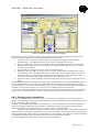
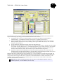
4.5.2 Selecting simulation targets
A simulation target specifies what performance parameter should be predicted after hitting the <Run> or <Find>
button. This can be noise margin or system margin, and when the modem is rate-adaptive (like for ADSL) you
can also select datarate or linerate. The simulation target can be set individually for each receiver model.
Figure 24 illustrates how to select the different simulation targets for an LT receiver from the GUI.
Figure 24: Selecting what performance parameter is to be simulated.
The options are Margin (Signal or Noise) and achievable Bit Rate (Line or Data):
• Noise Margin: Ratio (Pn2/Pn1) by which the received noise power Pn1 may increase to power Pn2 until
the recovered signal no longer meets the predefined quality criteria. This ratio is commonly expressed
in dB.
• Signal Margin: Ratio (Ps1/Ps2) by which the received signal power Ps1 may decrease to power Ps2 until
the recovered signal no longer meets the predefined quality criteria. This ratio is commonly expressed
in dB. In most practical situations, the signal margin is very close to the noise margin.
• Line Rate: The raw bitrate transported over the line, and includes all overhead needed for error
correction. Line Rate is always a “few percent” higher then the Data Rate.
Page 26 / 81
TNO 2009 - SPOCS 6.0, User Guide
•
Data Rate: The payload bitrate transported over the line, without any overhead needed for error
correction. Data Rate is always a “few percent” lower then the Line Rate.
You will find 2 options for each Margin alternative (no matter if we are dealing with Noise or Signal). These 2
options are Line Rate and Data Rate. In turn, if you prefer using Data Rate or Line Rate, you will also have 2
options. All the possibilities are summarized below.
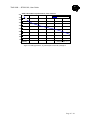
TARGET PARAMETER
Fixed @
Noise Margin
Description
Calculates the Data Rate at the Noise Margin set by
Data Rate
the user
Signal
Margin
Calculates the Data Rate at the Signal Margin set by
Data Rate
the user
Noise
Margin
Calculates the Line Rate at the Noise Margin set by
Line Rate
the user
Signal
Margin
Calculates the Line Rate at the Signal Margin set by
Line Rate
the user
Data
Rate
Calculates the Noise Margin at the Data Rate set by
Noise Margin
the user
Line Rate
Calculates the Noise Margin at the Line Rate set by
Noise Margin
the user
Data Rate
Calculates the Signal Margin at the Data Rate set by
Signal Margin
the user
Line
Rate
Calculates the Signal Margin at the Line Rate set by
Signal Margin
the user
REMARK (Target Parameters): the TARGET parameters are Margin (Signal or Noise) and Bit Rate
(Line or Data). The others are considered PROPERTIES of the receiver model.
Figure 25: Target Parameters in SPOCS.
4.6
Running performance calculations (SPOCS/full only)
To prepare SPOCS for a performance calculation, start defining a scenario of interest with a (victim) modem pair
under study, a disturber mix and associated loops. In this section, we will concentrate on what has to be added to
enable performance calculations like attainable bitrate, noise margin and reach.
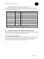
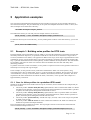
4.6.1 Running bit rate calculations
The attainable bit rate of a modem under study (=victim) is a number that is specified for a given margin and
loop length. It tells the maximum bitrate that can still be transported when the signal to noise ration deteriorates
by a given value (=margin). The usual way to present it is by means of a curve, as a function of the loop length.
This makes that we have to sweep the value for the loop length, and to fix the value for the margin.
Figure 26 highlights the relevant steps to enable such a bit rate calculation.
Page 27 / 81
TNO 2009 - SPOCS 6.0, User Guide
Figure 26: Relevant settings for a bitrate calculation.
Start defining a scenario of interest with a (victim) modem pair under study, a disturber mix and associated
loops. The following steps bring you the attainable bitrate for such a scenario:
• [A] Instruct the LT receiver to evaluate bitrates, by selecting DataRate or LineRate as simulation target.
The difference between these options is explained in section 4.5.2. Mark that this is only possible for
modems that are rate adaptive (such as for instance ADSL and VDSL). It is impossible to do that for
fixed bitrate modems (such as for instance SDSL and HDSL) since the concept of “attainable bitrate” is
meaningless for a fixed bitrate modem.
• [B] Once the simulation target is set to bitrate, the GUI will automatically switch to the associated
margin parameter (noise margin or signal margin). A commonly used value for margin is 6 dB, but you
can overrule it with other values.
• [C] Do exactly the same for the receiver at the other side of the loop
• [D] Specify the loop length as a value that has to be swept. Simply define the length as the result of
sweep parameter “k1”, and subsequently define a proper sweep. In the example of figure 26, we have
defined the sweep as “[100:100:5000]” meaning a sweep starting with “100”, ending with “5000”, in
steps of 100. The result is that the loop length sweeps from 100 meter to 5 km.
• [E] Hit the <RUN> button and SPOCS will evaluate and show you the attainable bitrate as function of
the loop length.
Mark that the performance is presented as a function of the sweep parameter “k1”. In this example it represents
the loop length, but SPOCS is not restricted to that. SPOCS has generalized this concept and you can use the
sweep parameter “k1” in any field of the frontpage of the GUI. For instance at a field that defines the number of
disturbers, or the crosstalk coupling. You can even use k1 at different places at the same time.
As soon k1 has been used somewhere, SPOCS will sweep it and produce a performance plot, otherwise SPOCS
evaluates only a fixed performance value. More details on the sweep parameter can be found in section 4.2.5.
.
4.6.2 Running margin calculations
The margin of a modem under study (=victim) is a number that is specified for a given bit rate and loop length. It
tells the amount of dB the signal to noise ration can deteriorate before the modem link gets unreliable. The usual
way to present it is by means of a curve, as a function of the loop length. This makes that we have to sweep the
value for the loop length, and to fix the value for the bitrate.
Figure 27 highlights the relevant steps to enable such a margin calculation.
Page 28 / 81
TNO 2009 - SPOCS 6.0, User Guide
Figure 27: Relevant settings for a margin calculation.
Start defining a scenario of interest with a (victim) modem pair under study, a disturber mix and associated
loops. The following steps bring you the attainable bitrate for such a scenario:
• [A] Instruct the LT receiver to evaluate margin, by selecting noise margin or signal margin as
simulation target. The difference between these options is explained in section 4.5.2.
• [B] Once the simulation target is set to margin, the GUI will automatically switch to the associated
bitrate parameter (data rate or line rate). Initially you will get a default value, but you can overrule it
with your value of interest.
• [C] Do exactly the same for the receiver at the other side of the loop
• [D] Specify the loop length as a value that has to be swept. Simply define the length as the result of
sweep parameter “k1”, and subsequently define a proper sweep. In the example of figure 27, we have
defined the sweep as “[100:100:5000]” meaning a sweep starting with “100”, ending with “5000”, in
steps of 100. The result is that the loop length sweeps from 100 meter to 5 km.
• [E] Hit the <RUN> button and SPOCS will evaluate and show you the margin as function of the loop
length.
Mark that the performance is presented as a function of the sweep parameter “k1”. In this example it represents
the loop length, but SPOCS is not restricted to that. SPOCS has generalized this concept and you can use the
sweep parameter “k1” in any field of the frontpage of the GUI. For instance at a field that defines the number of
disturbers, or the crosstalk coupling. You can even use k1 at different places at the same time.
As soon k1 has been used somewhere, SPOCS will sweep it and produce a performance plot, otherwise SPOCS
evaluates only a fixed performance value. More details on the sweep parameter can be found in section 4.2.5.
4.6.3 Running reach calculations
The reach of a modem pair under study (=victim) is a number that is specified for a given bit rate and noise
margin. It tells the longest loop length on which the modem pair can be deployed if it has to operated for a given
bit rate and at least 6 dB noise margin.
The reach is fixed number that holds for a link, and not for an individual modem. If downstream operates for a
certain loop length at 6 dB margin, and upstream at 2 dB margin, then the loop length is beyond the reach.
Therefore reach means that both modems have to operate under at least 6 dB margin.
Reach has to be evaluated in an iterative manner, and has to take the margin of the modems at both ends
of the loop under consideration. This makes that we have to tell SPOCS to do an iterative search to find beyond
what length the margin condition does not hold anymore for one of the two. This iteration is constrained between
a minimum and maximum value, and that a solution may not exist between these limits.
Figure 28 highlights the relevant steps to enable such a reach calculation.
Page 29 / 81
TNO 2009 - SPOCS 6.0, User Guide
Figure 28: Relevant settings for a reach calculation.
Start defining a scenario of interest with a (victim) modem pair under study, a disturber mix and associated
loops. The following steps bring you the attainable bitrate for such a scenario:
• [A] Instruct the LT receiver to evaluate margin, by selecting noise margin or signal margin as
simulation target. The difference between these options is explained in section 4.5.2.
• [B] Once the simulation target is set to margin, the GUI will automatically switch to the associated
bitrate parameter (data rate or line rate). Initially you will get a default value, but you can overrule it
with your value of interest.
• [C] Do exactly the same for the receiver at the other side of the loop
• [D] Specify the loop length as a value that has to be swept during the iteration. Simply define the length
as the result of sweep parameter “k1”, and subsequently define a proper sweep interval. In the example
of figure 28, we have defined the sweep as “[100:100:5000]” meaning an iterative search between
min(k1)=100 and max(k1)=5000. The value for step is irrelevant and will be ignored
• [E] Hit the <FIND> button and SPOCS will iterate k1 within the specified interval and returns the
maximum length for which both modems can operate under at least 6 dB margin. SPOCS warns you if
no solution can be found. In that case, extend the interval and try again.
Mark that the reach is iterated for the sweep parameter “k1”. In this example it represents the loop length, but
SPOCS is not restricted to that. SPOCS has generalized this concept and you can use the sweep parameter “k1”
in any field of the front page of the GUI. For instance at a field that defines the number of disturbers, or the
crosstalk coupling. You can even use k1 at different places at the same time. More details on the sweep
parameter can be found in section 4.2.5.
NOTE (Reach): When calculating the Reach, the user has to choose Margin (Signal or Noise) as
TARGET parameter, at a fixed Bit Rate (Line or Data).
Page 30 / 81
TNO 2009 - SPOCS 6.0, User Guide
5 Application examples
This section describes SPOCS functionalities and user interface by going step by step through some basic to
more advanced examples. They are additionally to the quick start examples discussed in section 3. These (and
other) examples can be found in the directory:
<InstallDir>\Examples\examples_manual.
Once SPOCS is started, you can load your first example scenario via the menu.
[FILE | LOAD] → select <InstallDir>\Examples\examples_manual\xxx.ssf
To make that directory the current directory, for easy loading other scenarios in the same directory, you use the
menu:
[FILE | FOLLOW DIRECTORY]
5.1
Example 1: Building noise profiles for ETSI tests
ETSI has defined various performance tests for ADSL to prove that the performance of a modem can meet their
minimum performance objectives, as specified in ETSI TS 101 388. It has to be verified for a range of stress
scenarios (4 different noise models, to be applied to 8 different test loops), and a range of payload bitrates. Each
combination of noise, loop and bitrate has its own reach requirements, specified as the (electrical) length of the
loop. Upstream and downstream are tested separately, and have different reach requirements. The noise models
are assumed to represent near worst-case scenarios where the modems share the cable with many other
(disturbing) modems.
To perform such a test in a lab environment, a noise profile is required to instruct a noise generator what noise it
should inject in test loop with a given length.
In this example, we will generate a noise profile that is dedicated for ADSL over POTS systems, using
overlapping spectra (this is called ADSL ‘annex A’ in the associated ITU standard). We will restrict our self to
“noise model FA”, test loop #2, and the bitrates 2.048 kb/s (downstream) and 512 kb/s (upstream). The reach
requirements for these combinations are almost the same (≈3225 down, ≈3275 up) and in this example it is
approximated by 3250 meter.
5.1.1 Case 1a: Noise profiles via a predefined ETSI model
SPOCS has all these ETSI noise models and test loops in its libraries, and we assume for this example that you
have access to them.
• The library model “TPL.dn:ADSL[007:255]-(SpM-2,POTS)" refers to downstream ADSL over POTS.
All DMT carriers between 7 and 255 are used for downstream transmission, and the model is specified
in SpM-2, the ETSI spectral management standard TR 101 830-2
• The library model “TPL.up:ADSL[007:031]-(SpM-2,POTS)" refers to upstream ADSL over POTS.
All DMT carriers between 7 and 31 are used for upstream transmission, and the model is specified in
SpM-2, the ETSI spectral management standard TR 101 830-2
• The library model “[ETSI.ADSL#2] = standard test loop: (0.5 mm)” refers to test loop #2 as specified
by ETSI in TS 101 388.
• The library model “MIX.dn:X.LT.FA” refers to ETSI noise model FA for ADSL over POTS, and
models the equivalent of multiple disturbers.
Figure 29 illustrates how to define the scenario. The loop length is fixed at 3250 m for the selected bitrates.
You can load this example scenario via:
[FILE | LOAD] → select <InstallDir>\Examples\examples_manual\Example1(caseA).ssf
Page 31 / 81
TNO 2009 - SPOCS 6.0, User Guide
Figure 29: Relevant settings for generating an ETSI noise profile.
On SPOCS/light only:
The noise profile is calculated and written to file after hitting the button <Generate LT noise profile>. To
inspect what spectra will be written, you should hit the button <Show Spectra>.
An alternative is right-clicking your mouse when it is above the <Generate LT noise profile> button. A
context menu pops-up, and one of its menu items is named “Noise inspector”. This will also provide the
spectrum that will be written to file after hitting <Generate LT noise profile>.
On SPOCS/full only:
The noise profile is calculated and written to file after hitting the button <Generate LT noise profile>.
To inspect what will be written, right-click your mouse when it is above the <Generate LT noise profile>
button. A context menu pops-up, and one of its menu items is named “Noise inspector”. This will show the
spectrum that will be written to file after hitting <Generate LT noise profile>.
An alternative is to enable the show of spectra, as shown below. Each time you hit the <run> button, the spectra
will be shown.
[FILE | VIEW | SHOW SPECTRA] → activated
Furthermore you may consider disabling the drawing of all curves in the plot, except to one for noise. This is
shown in figure 30. When you hit the <RUN> button, SPOCS will draw the curves in figure 31 and 32.
Figure 30: Selecting what curves are to be drawn in a spectral plot.
Page 32 / 81
TNO 2009 - SPOCS 6.0, User Guide
ETSI Noise profile on LT side, generated via noise model FA
-70
PSD [dBm/Hz]
v ia ETSI noise model FA
-80
[1]
-90
-100
-110
-120
-130
[SPOCS]
-140
Freq [Hz]
0
500k
1M
1.5M
2M
2.5M
Figure 31: Shape of the generated noise profile at the
LT side of the loop (for upstream performance testing).
ETSI Noise profile on NT side, generated via noise model FA
-70
PSD [dBm/Hz]
v ia ETSI noise model FA
-80
[1]
-90
-100
-110
-120
-130
[SPOCS]
-140
0
Freq [Hz]
500k
1M
1.5M
2M
2.5M
Figure 32: Shape of the generated noise profile at the
NT side of the loop (for downstream performance testing).
WARNING: The above mentioned noise profile generated by SPOCS will be a slightly different
from what is defined by ETSI in TS 101 388. This is because ETSI has updated its preferred way
to incorporate length-dependencies in the evaluation of crosstalk coupling. TS 101 388 (ADSL)
requires that the evaluation of the involved transmission function, named STO(f, L), is to be
normalized against an “average” 135 ohm (knowing that ADSL is a 100 ohm system), while the
more recent TR 101 830-2 (Spectral Management) recommends to normalize it against the
characteristic impedance of the loop. SPOCS follows the latter, because it provides consistent
results among different scenarios, but it will result in a (minor) difference with TS 101 388.
However if this difference is relevant for compliance testing, we recommend to use noise profiles
that are fully dedicated to a particular standard of interest. They can account for all these
“inconsistencies” between different standards.
Page 33 / 81
TNO 2009 - SPOCS 6.0, User Guide
5.1.2 Case 1b: Noise profiles via a disturber mix
SPOCS brings you that ability to generate noise profiles form arbitrary scenario’s, and not only for a limited
number of noise models and test loops of a standard. The ETSI noise models are to represent a mix of disturbers,
and noise model FA originates from a high penetration scenario. It was modelled for a mix using 400 wire pairs
in a 900 wire-pair cable (90×ISDN + 40×HDSL/2 + 180×ADSL + 90×SDSL) as described in:
• Brink, FSAN: Realistic ADSL noise models, ETSI contribution 994t37a0, dec 1999.
• Brink, Heuvel, FSAN: Update of SDSL noise models, as requested by ETSI-TM6, ETSI contribution
993t22a0, sept 1999.
Figure 33 illustrates how to configuration the scenario if equivalent noise model “ETSI-FA” is replaced by 400
individual disturbers. You can load this example scenario via:
[FILE | LOAD] → select <InstallDir>\Examples\examples_manual\Example1(caseB).ssf
The resulting noise profile will not be exactly the same as for the ETSI noise model, since it depends also on the
assumptions being made about the PSD’s of these individual disturbers. These assumptions have been changed
over the years, and the models used in figure 33 are the most recent ones, and defined in the ETSI Spectral
Management standard TR 101 830-2.
Figure 34 and 35 show the resulting noise profile, as well as the one obtained via the ETSI noise model FA.
These profiles are not the same (but close), so the use of a disturber mix is not suitable for compliance testing.
However, the noise profiles generated via a disturber mix are not only closer to what can be expected in reality;
their definition is also closer to what they actually represent.
Figure 33: Generating a noise profile via a disturber mix.
Page 34 / 81
TNO 2009 - SPOCS 6.0, User Guide
ETSI Noise profile on LT side, approximated via a disturber mix
-70
PSD [dBm/Hz]
v ia ETSI noise model FA
-80
[1]
[1]
-90
-100
-110
-120
-130
[SPOCS]
-140
0
Freq [Hz]
500k
1M
1.5M
2M
2.5M
Figure 34: Shape of a noise profile generated from a disturber mix,
at the NT side of the loop (for downstream performance testing).
ETSI Noise profile on NT side, approximated via a disturber mix
-70
PSD [dBm/Hz]
v ia ETSI noise model FA
-80
[1]
[1]
-90
-100
-110
-120
-130
[SPOCS]
-140
0
Freq [Hz]
500k
1M
1.5M
2M
2.5M
Figure 35: Shape of a noise profile generated from a disturber mix,
at the NT side of the loop (for downstream performance testing).
Page 35 / 81
TNO 2009 - SPOCS 6.0, User Guide
5.2
Example 2: Performance calculation of ADSL over POTS
(SPOCS/full only)
The profile of the previous example enables performance testing for a single loop length, and repeating that for
various lengths can by quite time consuming. SPOCS enables you to calculate this quickly for a range of loop
length, and this example explain how.
5.2.1 Case 2a: Margin calculation of ADSL over POTS
Figure 36 shows how to change the scenario from the previous example (see figure 33) with a fixed loop length,
into a scenario with variable loop length that can be swept in length. The circles and arrows illustrate what has
been added: the loop length is replaced by the sweep parameter k1, that is instructed to sweep from 250 meter to
4000 meter in steps of 250 meter (see section 4.2.5 for further details). By hitting the <RUN> button, SPOCS
will calculate the noise margin for all values of the sweep parameter, in both transmission directions.
You can load this example scenario via:
[FILE | LOAD] → select <InstallDir>\Examples\examples_manual\Example2(caseA).ssf
To speed-up the calculation process, it is recommended to de-activate the presentation of intermediate spectra:
[FILE | VIEW | SHOW SPECTRA] → de-activate
Figure 36: A scenario for calculating the margin of
ADSL over POTS as a function of the loop length.
Figure 37 shows the results in a plot, and figure 38 shows the same in a tabular format. The plot shows that the
margin drops with the loop length, and that the downstream margin is often a few dB better than for upstream.
When the length exceeds about 3 km then the upstream margin drops below 6 dB. This is the reach for this
bitrate combination. Beyond that length, the system will operate, but upstream may become unreliable.
If you hit the <FIND> button, SPOCS will evaluate that reach for you, and returns a value of about 3084 m.
Page 36 / 81
TNO 2009 - SPOCS 6.0, User Guide
Performance Plot
30
[dB]
[1] N_Margin Up
[2] N_Margin Dn
25
[1] [2]
20
15
10
5
0
[SPOCS]
-5
0
500
Sweep Parameter
1k
1.5k
2k
2.5k
3k
k1 -->
3.5k
4k
Figure 37: The margin of ADSL over POTS as a function of the loop length,
when it operates under the stress conditions of the scenario defined in figure 36.
Figure 38: The same margin of ADSL over POTS as
shown in figure 37, but now in a tabular format.
Page 37 / 81
TNO 2009 - SPOCS 6.0, User Guide
5.2.2 Case 2b: Bitrate calculation of ADSL over POTS
The observation that the downstream margin is a few dB above the upstream margin means that the downstream
bitrate can be increased without reducing the reach. Additionally, on shorter loops the bitrate can increase for
both directions if 6 dB margin is considered as adequate. Figure 39 illustrates how to change the scenario of
figure 36 for calculating the attainable bitrate as a function of the loop length.
The definition of the sweep parameter k1 remains unchanged, compared to figure 36. The only things that are to
be changed are the simulation targets at the receivers: they change from margin to bitrate (see section 4.5.2 for
further details).
You can load this example scenario via:
[FILE | LOAD] → select <InstallDir>\Examples\examples_manual\Example2(caseB).ssf
Figure 39: A scenario for calculating the margin of
ADSL over POTS as a function of the loop length.
Figure 40 shows the results in a plot, and figure 41 shows the same in a tabular format. The plot shows the
attainable bitrates as a function of the loop length if the modem has to operate with at least 6 dB noise margin.
These bitrates drop with the loop length, but on a distance of 3 km it is still possible to offer 3.05 Mb/s in
downstream and 528 kb/s in upstream under the assumed stress conditions.
Page 38 / 81
TNO 2009 - SPOCS 6.0, User Guide
9M
Performance Plot
[b/s]
[1] DataRate Up
8M
[2] DataRate Dn
[2]
7M
6M
5M
4M
3M
2M
1M
[1]
[SPOCS]
0
0
500
Sweep Parameter
1k
1.5k
2k
2.5k
3k
3.5k
k1 -->
4k
Figure 40: The attainable bitrate of ADSL over POTS as a function of the loop length,
when it operates under the stress conditions of the scenario defined in figure 39.
Figure 41: The same bitrates of ADSL over POTS as
shown in figure 40, but now in a tabular format.
Page 39 / 81
TNO 2009 - SPOCS 6.0, User Guide
5.2.3 Case 2c: Inspecting intermediate spectra
When SPOCS calculates performance, various intermediate results are evaluated, such as signal and noise
spectra. On default, these results are not shown, so you must enable this first via the following menu item:
[FILE | VIEW | SHOW SPECTRA] → activated
If you reload and run the example scenario 1b in figure 33 (or replace the loop length by a fixed number of
3250m) then SPOCS will show the spectra in figure 42 and 43 as well. On default, 3 curves will be shown:
• 1: The transmit signal, as transmitted on the other side of the loop.
• 2: The receive signal, as observed at the input of the receiver under test.
• 3: The noise, as observed at the input of the receiver under test.
The distance between receive and transmit curves is the cable loss in dB. The distance between the received
signal and noise curve is the signal to noise ratio. This area is highlighted by the green lines, because it is a fair
measure for the maximum bitrate. If you use some imagination and increase the noise by 6 dB, then the
remaining area reduces. This will be a fair measure for the attainable bitrate at 6 dB noise margin.
You can make more curves visible (or disable most of them) by selecting the curves of interest via the menu
item:
[FILE | VIEW | SELECT SPECTRA] → activate/deactivate what is needed
NT spectra: Downstream signal, received noise
-20
PSD [dBm/Hz]
-40
[1] Transmitted Signal, @100 ohm
[1]
[2] Receiv ed Signal, @100 ohm
[3] Receiv ed Noise, @100 ohm
-60
[2]
-80
[3]
-100
-120
-140
-160
-180
[SPOCS]
-200
0
Freq [Hz]
500k
1M
1.5M
2M
2.5M
Figure 42: The downstream receiver will observe these spectra at the
NT side of the loop, if it is part of the scenario shown in figure 33.
Page 40 / 81
TNO 2009 - SPOCS 6.0, User Guide
LT spectra: Upstream signal, received noise
-20
PSD [dBm/Hz]
[1]
-40
[1] Transmitted Signal, @100 ohm
[2] Receiv ed Signal, @100 ohm
[3] Receiv ed Noise, @100 ohm
-60
-80
[3]
-100
-120
[2]
-140
-160
-180
-200
[SPOCS]
-220
Freq [Hz]
0
500k
1M
1.5M
2M
2.5M
Figure 43: The downstream receiver will observe these spectra at the
NT side of the loop, if it is part of the scenario shown in figure 33.
If you make a sweep through various loop lengths, as used in example 2b shown in figure 39, then you will see
multiple spectra as well. This will slow-down the calculation speed significantly, and therefore these plots are
disabled by default. Figure 44 and 45 show the spectra in case the loop length is swept.
NT spectra: Downstream signal, received noise
-20
PSD [dBm/Hz]
-40
[1]
-60
-80
[1] Transmitted Signal, @100 ohm
[2]
[2]
[2]
[2]
[2]
[2]
[2]
[2]
[2]
[2]
[2]
[2]
[2]
[2]
[2]
[2]
[2] Receiv ed Signal, @100 ohm
[3] Receiv ed Noise, @100 ohm
[3]
[3]
[3]
-100
-120
-140
-160
-180
-200
[SPOCS]
-220
0
Freq [Hz]
500k
1M
1.5M
2M
2.5M
Figure 44: The downstream receiver will observe these spectra at the
NT side of the loop, if the loop length is swept (see figure 39).
Page 41 / 81
TNO 2009 - SPOCS 6.0, User Guide
LT spectra: Upstream signal, received noise
0
PSD [dBm/Hz]
[1] Transmitted Signal, @100 ohm
[2] Receiv ed Signal, @100 ohm
[1]
[3] Receiv ed Noise, @100 ohm
-50
[3]
[2]
[2]
[2]
[2]
[2]
[2]
[2]
[2]
[2]
[2]
[2]
[2]
[2]
[2]
[2]
[2]
-100
-150
-200
[SPOCS]
-250
0
Freq [Hz]
500k
1M
1.5M
2M
2.5M
Figure 45: The downstream receiver will observe these spectra at the
NT side of the loop, if the loop length is swept (see figure 39).
5.3
Example 3: Impact Analysis of VDSL2 on ADSL2plus
(SPOCS/full only)
An impact analysis is a study of the consequences when new technology is introduced in an access network. For
instance, introducing the deployment of VDSL2 from a cabinet (the “new” technology) in a network where all
deployments are from the central office (‘the “legacy”). The impact analysis should answer the question whether
the legacy will be disturbed by the new technology in a disproportional manner or not, and if yes how much.
Such a study compares the performance result under different scenarios that are considered as “equivalent”. This
means that all scenarios serve the same number of customers, and one of them (the “reference” scenario)
represents the legacy situation.
This example 3 illustrates how to do that, assuming ADSL2plus from the central office as “legacy” and VDSL2
from street cabinets as “new technology”. It requires some advanced features of SPOCS, which become
available when you increase the level of expertise to “advanced” via the CONFIG menu. See section 6.1 for
further details.
At first, we need to define a loop topology with multiple sections, as explained before in section 4.2.1. Secondly
we need a way to modify that scenario in such a way that the location of the street cabinet and the number of
VDSL2 systems can be varies in a convenient manner. All these scenarios have to be equivalent, meaning that
the number of systems remains the same for all those scenarios.
This is where the use of the constants “k2” and “k2” becomes convenient, and the use of expressions becomes
powerful (see section 4.2.5 and 4.2.1). Figure 46 shows how we can define all scenarios by varying only the
values of constant “k2” and “k3”. Figure 47 illustrates a few values of interest being used in this example. If you
push the <SHOW> button, SPOCS will provide you with a graphic summary of the scenario, as shown in figure
48.
You can load this example scenario from disk, and to modify “k2” and “k3”.
[FILE | LOAD] → select <InstallDir>\Examples\examples_manual\Example3.ssf
Page 42 / 81
TNO 2009 - SPOCS 6.0, User Guide
Figure 46: Defining a range of scenarios by using k2 for the cabinet position and k3 for the
number of VDSL2 systems. The total number of disturbers is always kept at 200.
Scenario
Loop sections
k1=Sweep parameter
k2=Location of the cabinet
k3=Number of VDSL2 systems
#1=ref
#2
#3
#4
#5
[k2, k1-k2]
[max(100,k2) : 50 : 5000]
0
2000 2000 1500 1000
0
1
50
50
50
Figure 47: By changing the values for “k2” and “k3”, we can
easily analyze different variants of the scenario in figure 46.
Loop ran ge: [k2, k1-k2] →
(2000 m ...
(Only the maximum values are drawn below)
5000 m)
[SPOCS]
2000
3000
DSLAM
[LT]
[1]
[2]
[3]
← <up stream>
CPE
[NT]
<downstream> →
V:
D1:
D2:
LOOP:
V = Victim,
D = Disturber,
[KPN_L1]
= undergroun d cable L1 ( 50×4×0.5mm), 0.5km
[1]..[3] = NodeNumber
NEXT = -50 dB[1Mhz],
V.t = TPL.dn:ADSL2+/A-[033:511]-(G992.5,FDD)
V.r = ADSL2+/A.up[FDD]-(expert guess)
D1 = TPL.dn:ADSL2+/A-[033:511]-(G992.5,FDD)
D2 = TPL.dn:VDSL2.B7-5-(8a,997-M2x-A)
D3 = Noise:White(-140dBm/Hz)
EL-FEXT = -45 dB[1Mhz,1km]
V.t = TPL. up:ADSL2+/A-[ 007:031]-(G992.5)
V.r = ADSL2+/A.dn[FDD]-(expert guess)
200-k3 #
k3 #
1#
D1 = TPL. up:ADSL2+/A-[ 007:031]-(G992.5)
D2 = TPL. up:VDSL2. B7-5-(8a,997-M2x-A)
D3 = Noise:W hite(-140dBm/Hz)
200-k3 #
k3 #
1#
Figure 48: Graphic representation of the scenario in
figure 46, obtained via the <SHOW> button.
Figure 49 and 50 shows the results from sequential simulations. Results from sequential runs can be kept in a
single plot if the plots are “hold” in-between. This behaviour can be toggled via the menu item:
[VIEW | HOLD PLOTS, WHEN RECALCULATED]
The first figure (49) shows a significant impact if the first VDSL2 modem is deployed from a cabinet (you have
to “shape” the PSD of VDSL2 to prevent this, but that is beyond the scope of this example). Adding more and
more VDSL2 modems will have an additional impact, but not as extreme as the first one. Note that this is only
Page 43 / 81
TNO 2009 - SPOCS 6.0, User Guide
true in a statistical sense. In 99% of the cases the impact will not be so severe as shown in figure 49 but this
severity can happen in practice.
The second figure (50) shows that when the cabinet location is changed that the severity in impact will change as
well, but it remains significant (and probably unacceptable in most operational cases).
16M
Impact ofVDSL2 on ADSL2plus dow nstream performance
[b/s]
[1] ref erence (ADSL2plus Only )
[2] 1 VDSL2 disturber at 2000m
14M
[3] 50 VDSL2 disturbers at 2000m
[1]
12M
10M
8M
6M
[2]
4M
[3]
2M
[SPOCS]
0
0
500
Sweep Parameter
1k
1.5k
2k
2.5k
3k
3.5k
4k
k1 -->
4.5k
5k
Figure 49: Deploying only one VDSL2 system from a cabinet (without proper measures)
can have a severe negative impact on ADSL2plus deployments from the exchange.
16M
Impact of VDSL2 on ADSL2plus downstream performance
[b/s]
[1] ref erence (ADSL2plus Only )
[2] 50 VDSL2 disturbers at 2000m
14M
[3] 50 VDSL2 disturbers at 1500m
[1]
[4] 50 VDSL2 disturbers at 1000m
12M
10M
8M
6M
[4]
4M
[3]
[2]
2M
[SPOCS]
0
0
500
Sweep Parameter
1k
1.5k
2k
2.5k
3k
3.5k
4k
k1 -->
4.5k
5k
Figure 50: Changing the location of the cabinet will change the amount of eploying only
one VDSL2 system from a cabinet will have a significant negative impact on ADSL2plus
deployments from the exchange (unless proper measures are taken).
Page 44 / 81
TNO 2009 - SPOCS 6.0, User Guide
5.4
Example 4: Branching, ADSL and VDSL (SPOCS/full only)
It is a common approach in performance studies to keep the involved topology as simple as possible. Many
VDSL2 studies assumed a straight loop where all customers are at the end of the line, or distributed along the
line, as shown in figure 51.
Street
Central office
ADSL
cabinet
Customers
#1
#2
#3
VDSL
Figure 51: An over-simplified topology, assuming all customers distributed along the same
loop.
Real-life topologies, however, are not like straight loops: they are branched. It is common in the Netherlands
that a 900-wire-pair distribution cable leaves the central office, to arrive in a street cabinet. From thereon, the
cable fans out into nine 100 wire-pair cables. SPOCS has the capability to include branching in your scenario,
and the example below show why you need it (and cannot make good simulations without it).
Figure 52 illustrate a few topologies where 360 broadband systems are deployed to a single distribution area.
• Case A is a simple (straight) topology, assuming that all customers are (virtually) collocated at the end
of the loop. It represents the “classic” approach of describing a topology.
• Case B is a branched topology that represents the same real-world topology, but in an improved
manner. The 360 ADSL systems fan out from the street cabinet into 9×40 branches. Each branch
transports 40 ADSL systems, and does not couple any crosstalk into another branched. As a result, the
predicted performance is somewhat higher then in case A, since case A is too pessimistic.
• Case C is the same branched topology as in case B, but now we have moved 180 systems from the
central office (ADSL) to the street cabinet (VDSL) so that the same number of customers are being
served. VDSL however is branched as well into 9×20 branches , so only 20 of them share the branch of
the ADSL systems under study. The rest does not contribute to the received crosstalk.
• Case D is almost the same as case C with the difference that case D is to study VDSL performance.
Mark that VDSL is disturbed by only 20 ADSL systems in the same branch, and not by the 180 ADSL
systems from the central office.
Street
Central office
Customers
cabinet
Case A:
360 ADSL
360 ADSL
Street
Central office
cabinet
Case B:
40 ADSL
360 ADSL
Street
Central office
cabinet
Case C:
20 ADSL
Case D:
20 VDSL
180 ADSL
180 VDSL
Figure 52: Topologies being analyzed in example 4.
Page 45 / 81
TNO 2009 - SPOCS 6.0, User Guide
This example 4 illustrates how to instruct SPOCS to do these studies. It requires some advanced features of
SPOCS, which become available when you increase the level of expertise to “advanced” via the CONFIG
menu. See section 6.1 for further details.
You can load this example scenario from disk:
[FILE | LOAD] →
[FILE | LOAD] →
[FILE | LOAD] →
[FILE | LOAD] →
select <InstallDir>\Examples\examples_manual\Example4(CaseA).ssf
select <InstallDir>\Examples\examples_manual\Example4(CaseB).ssf
select <InstallDir>\Examples\examples_manual\Example4(CaseC).ssf
select <InstallDir>\Examples\examples_manual\Example4(CaseD).ssf
You can inspect these scenarios one for one, to see how branching and power back-off have been applied. When
the PBO button colours red you can inspect the amount of PBO for that disturber/transmitter by right-clicking its
PBO button. A context menu will then pop up, and one of its menu items is the PBO inspector.
Figure 53 illustrates the ADSL bitrates as evaluated for case A, B and C.
• Curve A is below B since the topology without branching is too pessimistic. Ignoring branching for
ADSL studies can easily result in predictions that are 10-15% too pessimistic.
• Curve C is above B since the PBO settings has shaped VDSL2 “too deep”. It would require an
adjustment of the PBO settings to make curve C and B similar, but this is out of scope of this example.
Figure 54 illustrates the VDSL bitrates for street cabinets positioned at 2km distance from the central office.
14M
ADSL2plus downstream performance, from exchange
[b/s]
[1] classic prediction
[2] branched, without VDSL
12M
[3] branched, with shaped VDSL
[2] [3]
10M
[1]
8M
6M
4M
2M
0
[SPOCS]
0
500
Sweep Parameter
1k
1.5k
2k
2.5k
3k
3.5k
4k
4.5k
k1 -->
5k
Figure 53: ADSL performance, as predicted from the scenarios A, B and C of example 4.
Page 46 / 81
TNO 2009 - SPOCS 6.0, User Guide
50M
VDSL2 downstream performance, from cabinet
[b/s]
[1] branched prediction
45M
[1]
40M
35M
30M
25M
20M
15M
10M
5M
0
[SPOCS]
0
Sweep Parameter
200
400
600
800
1k
k1 -->
1.2k
Figure 54: VDSL performance, as predicted from scenario D of example 4.
Page 47 / 81
TNO 2009 - SPOCS 6.0, User Guide
6 Using Advanced Features
6.1
Selecting different levels of expertise
The list of possible models can be overwhelming, and this is not always favourable. SPOCS enables the use of
different expertise modes, namely, Basic, Advanced and Expert, to reduce the list of models on a user request.
You can easily switch between these modes via the Config menu, as shown in figure 55.
Figure 55: Working in the advanced level of expertise is the recommended
level for many studies, and gives access to tuneable models.
The recommended level to work with is the Advanced level, but beginners can take advantage from starting
SPOCS in the Basic level. The default choice on start-up is the Basic level, but this default can easily be changed
by customizing the configuration file, as explained in the annex C.
The difference between the levels are roughly as follows:
• Basic level (recommended only for beginners)
o transmitter/disturber models are limited to the most relevant once
o model parameters cannot be changed
o values for NEXT and FEXT cannot be changed
o parameter k2 and/or k3 cannot be used
• Advanced level (recommended for common use)
o Access to all relevant transmitter/disturber models (PSD templates)
o Access to tuneable models, if you want to change some model parameters
o NEXT and FEXT can be changed from the GUI
o Parameters k2 and k3 can be used on top of the sweep parameter k1
• Expert level (discouraged, unless you know exactly what you are doing)
o Access to all transmitter/disturber models defined in the library (overwhelming)
§ Not only for PSD templates, but also for PSD masks
§ Using transmitters in the wrong direction (downstream modems in upstream)
NOTE: If you read a scenario, that contains models that are only available for higher levels of
expertise, SPOCS will raise an error. Simply increase the current level of expertise, and read it
again.
6.2
Using Power back-off models
DSL modems can be equipped with a mechanism, called power back off, that reduces their transmit power. It has
many purposes, including the reduction of power consumption, improving receiver dynamic range, reducing
crosstalk, etc. Power cut-back is a specific (simplified) variant of power back-off, characterized by a frequency
independent reduction of the in-band PSD. It is used, for instance, in ADSL and SDSL.
Detailed information on PBO is available via the Help menu of SPOCS.
6.2.1 Selecting a PBO model
On default, PBO is not applied. By hitting one of the PBO buttons a dialog box pops up to select a model of
choice. It is easy to verify if PBO is activated or not for a particular modem. The PBO buttons highlight in red if
any PBO model is selected. This is shown in figure 56.
Page 48 / 81
TNO 2009 - SPOCS 6.0, User Guide
Figure 56: The PBO button colours red if PBO is activated for that particular modem.
To find out in the dialogbox what each model means, select one and right-click on it with your mouse. This
opens a context menu, with an info entry, to provide you with basic information about the model. More info is
available via the overall Help menu of SPOCS.
Most of the PBO models have fixed parameter values, meaning that you cannot change their values. This
protects you from unattended changes. In special cases you may want to tweak one or more of these parameters.
Therefore, some of the models are made “tuneable” (only visible when working in the advanced level or higher,
as explained in section 6.1).
6.2.2 Available PBO models, and its parameters
The amount of power back-off may depend on fixed settings, on the insertion loss of the loop, on the level of the
received signal, or a mix of these. The model converts a “source signal” (generated by a transmitter model) into a
“transmit signal”, and that transmit signal is injected into the loop. This conversion is controlled by one or more
of the following values:
• the “source signal” spectrum, as provided by the transmitter model;
• the “source signal” spectrum of the modem at the other side of the loop (without PBO at the other side);
• the “characteristic transfer” of the loop being studied to account for attenuation
Different DSL standards have produced different PBO mechanisms, and therefore you can select a PBO model
from a list with many options (individually for each transmitter/disturber).
A complete list of PBO models and a description of its parameters can be found via the Help menu via:
Power back-off models
- index of all PBO models
- Selecting PBO models in downstream direction
- Selecting PBO models in upstream direction
6.2.3 Inspecting a PBO model
To find out how much a selected PBO model modifies a transmit signal, you can right-click on the PBO button
with your mouse. This opens a context menu, and one of its menu items is named “PBO Inspector”. Figure 57
illustrates the result of hitting that menu item: The upper curve represents the downstream transmit signal of a
VDSL2 system deployed from a street cabinet, before any PBO is applied. The lower curve represent what signal
level is injected into the loop after being shaped by the PBO model.
Page 49 / 81
TNO 2009 - SPOCS 6.0, User Guide
PBO-model = "PBO.dn:PSD_Shaping_ITU_EXPERIMENTAL"
Transmit-model = "TPL.dn:VDSL2.B8-4-(8a,998-M2x-A)"
Loop model = "[KPN_L1] = underground cable L1 ( 50×4×0.5mm), 0.5km"
Loop length = 500 m
-20
Transfer into 100 ohm [dB]
Source Spectrum (before PBO)
Transmit Spectrum (after PBO)
-40
-60
-80
-100
-120
-140
[SPOCS]
0
500k
Freq [Hz]
1M
1.5M
2M
2.5M
3M
3.5M
4M
4.5M
5M
Figure 57: The amount of power back-off can be visualized via the “PBO inspector”.
6.3
Using Receiver models (SPOCS/full only)
On default, the receiver model of a modem is auto-selected by SPOCS as soon as you select its transmitter. This
choice is often a good choice, and therefore (again on default) the GUI prevents you from changing this choice.
However in some cases there is a need to overrule the selection, for instance to (a) select another receiver model,
or (b) to change its parameter values.
6.3.1 Selecting an alternative Receiver Model
To select an alternative receiver model, different from the default choice, you have to disable the auto
completion mode for victim modems. You can deactivate it from the Config menu, via:
[ CONFIG | AUTO COMPLETION MODES | Keep victims paired ]
Now the listbox of the receiver becomes selectable, and you can select an appropriated one. The list of specific
receiver models is long enough to find a matching one for most modems that are conform some DSL standard. If
you are analyzing a non-standard but good-quality modem, using a line code that is unknown to you, then the
“Generic.DEFAULT” model may give fair simulation results.
To find out what each model means, select one and right-click on it with your mouse. This opens a context
menu, with an info entry, to provide you with basic information about the model. For more details, please check
the SpM-2 [1] standards of the model you are interested in.
Additional information can be found by pushing the <Parameters> button on the receiver box. It shows the
values of parameters being used. Each model has its own list of parameters, being a subset of the list shown
below:
GAP
Parameters of Receiver models
It corresponds to the effective Gap in Signal-To Noise Ratio NR-Gap. SNR-
Page 50 / 81
TNO 2009 - SPOCS 6.0, User Guide
NOISE
ECHOSUP
DISTSUP
RN
LINES
BITPERSYM
BITLOADRANGE
SYMBOLRATE
Gap is a performance parameter that indicates how close the detection
approaches the Shannon capacity limit. Roughly, the amount of dB that the
noise can increase before the link quality gets too low. It is often represented
by the symbol ΓdB.
Corresponds to the receiver noise, known as PRN0_dB (see clause 5.1 of [1]).
The fragment of the transmit signal that echoes into the receiver is usually
suppressed by an echo canceller. Some residual echo will always remain after
echo cancellation, adds like noise to the received signal, and reduces the
performance.
EchoSup is a parameter of a simple model to express what fraction of the
received echo has left (and will behave like noise). If set to “Inf”, it becomes
infinite, as if the echo cancellation were ideal
The received signal is distorted by cable loss, and the signal that was
transmitted is recovered from the received signal by means of an equalizer.
Usually, these equalizers are very effective, but not perfect. The restored
signal will always differ slightly from the transmitted signal, and this will also
add noise to the received signal, thus reducing the performance.
DistSup is a parameter of a simple model to express what fraction of the
transmitted signal is not recovered (and will behave like noise). If set to “Inf”,
it becomes infinite, as if the equalization were ideal
The impedance of the modem, and in use for both the transmitter and the
receiver. Changing the impedance changes the signal loss in a cable and the
echo.
Used in SDSL and HDSL. This is related to the use of capacity. For example,
if the total capacity were 5 Mbps, and, Lines is set to 2, this would mean that
the real capacity treated in SPOCS for calculations is equal to 2.5 Mbps.
Number of Bits per symbol.
These two values represent the minimum as well as the maximum number of
bits per tone per symbol.
Used in DMT systems (ADSL, VDSL2). A common choice used in ADSL
and VDSL systems is to set to 4000 baud/s.
FREQBANDS
Frequency Bands to be used. Used in the generic Shannon model.
CARRIERFREQ
The frequency carrier. Mostly used when working with CAP systems, i.e.
HDSL.CAP
FREQTONES
Used when working with DMT, corresponding to the set of sub-carriers. The
use and location of the freq-tones varies according to each product supporting
DMT.
The delta frequency is the spacing between DMT carriers Common value is
4,3125KHz, though in VDSL2 systems it may change to 8,625 KHz when
high frequencies are used
Impulse Noise Protection: This is a parameter used in ADSL2+ in order to
deploy a protection mechanism for the effect of impulse noise. There are
several tables on ref [3,4] from which the user can choose the symbols to be
used in conjunction with the delay.
Changing INP will change the amount of overhead (difference between the
LineRate and the DataRate)
This is a parameter used in ADSL2+ and provides in conjunction with INP
the mechanism to protect the system against Impulse Noise effect.
Changing Delay will change the amount of overhead (difference between the
LineRate and the DataRate)
Embedded Operational Channel-OverHead: This parameter has a range from
8-to-64 Kbps and is used for exchanging messages between the modems
DF
INP
DELAY
EOCOH
Figure 58: Understanding the parameter of the receiver models.
Page 51 / 81
TNO 2009 - SPOCS 6.0, User Guide
6.3.2 Selecting tuneable receiver models
Most of the receiver models have fixed parameter values, meaning that you cannot change their values. This
protects you from unattended changes. In special cases you may want to tweak one or more of these parameters,
for instance to account for a better noise gap or another amount of impulse noise protection. This is only possible
for the receiver models that are specifically intended to be tuneable.
To get access to one of the tuneable receiver models, you have to bring the level of expertise at least to the
“Advanced level”. Additionally, the auto completion mode should be switched-off for victims, so that you can
overrule the default receiver model by a tuneable model of your choice. You can change them both via the
CONFIG menu:
[ CONFIG | AUTOR COMPLETION MODE | KEEP VICTIMS PAIRED ] à “disabled”
[ CONFIG | LEVEL OF EXPERTISE | ADVANCED ]
Now the listbox of the receiver will contain tuneable models as well. To warn you that you have selected a
tuneable model, the GUI responds on it by highlighting the <Parameters> button from yellow to red.
Figure 59: Receiver Models in SPOCS: Fixed and Tuneable
Figure 60: The <PARAMETER> button colours red
if you have changed a parameter of a tuneable model.
The current version of SPOCS does not support that the sweep parameter k1 can be used in the
tuneable parameters, but such a capability is intended for a next revision of SPOCS.
Page 52 / 81
TNO 2009 - SPOCS 6.0, User Guide
6.3.3 Selecting a generic receiver model
The list of specific receiver models is long enough to find a matching one for most modems that are conform
some DSL standard. However in some cases this is not good enough and you may need to access one of the
generic receiver models that are beneath these specific models.
The ETSI SpM-2 standard [1] identifies several generic models for receiver performance, dedicated to different
line code principles. SPOCS supports the following generic models:
• Shifted Shannon, which is line code independent and therefore the most generic one.
• PAM, dedicated to line-codes using Pulse Amplitude Modulation.
• CAP/QAM, dedicated to line-codes using Quadrature modulation.
• DMT, dedicated to line-codes using multiple discrete tones.
These generic models are the basis for all specific models in the library, where each specific model has its own
set of parameter values.
These generic models … … are used in the following specific receiver models:
ISDN, SDSL, HDSL.2B1Q.
PAM
HDSL.CAP and VDSL1(CAP) –now obsoleteCAP
ADSL, VDSL2
DMT
Figure 61: Examples of DSL systems working based on the different generic models.
To get access to one of the generic receiver models, you have to bring the level of expertise to at least the
“Advanced level”. You can change this via the Config menu:
[ Config | Level of expertise | Advanced ]
Now the listbox of the receiver will contain generic receiver models as well. The parameters of these models are
all tuneable, and the following parameters apply to each model:
PROPERTIES
Gap
Noise
EchoSup
DistSup
Rn (Impedance)
Lines
BitPerSym
BitLoadRange
SymbolRate
FreqBands
CarrierFreq
FreqTones
dF
INP
Delay
EOCOH
SHANNON
x
x
x
x
x
x
PAM
x
x
x
x
x
x
x
CAP
x
x
x
x
x
x
x
DMT
x
x
x
x
x
x
x
x
x
x
x
x
x
x
Figure 62: General and Specific Properties of the Generic Models.
6.3.4 Inspecting a receiver model (bitloading)
To find out what bitloading a DMT model does with a transmit signal, right-click on the receiver list box with
your mouse. This opens a context menu, and one of its menu items is named “Receiver inspector”. Figure 63
illustrates the result of hitting that menu item: The dotted curve (rounded) is close to what bitloading an actual
Page 53 / 81
TNO 2009 - SPOCS 6.0, User Guide
modem would report under the stress conditions of your scenario. The solid curve (fractional) is the one being
used during calculations.
8
DMT Bit Loading diagram
Receiver Model = "ADSL/POTS.dn[EC]-(SpM-2)"
N_Margin = 5.38, DataRate = 2048.00 kb/s, Gap = 7.50 dB, NT-side
Bit Loading (bits/carrier)
Fractional (Linerate: 2350 kb/s)
Rounded
7
6
5
4
3
2
1
0
[SPOCS]
0
Frequency (MHz)
0.2
0.4
0.6
0.8
1
1.2
1.4
Figure 63: The bitloading can be visualized via the “receiver inspector”.
6.4
Adding user-definable models (SPOCS/full only)
SPOCS offers the functionality to add your own models to the libraries. This is a powerful mechanism to enable
you to keep the list of SPOCS models up-to-date with the developments in standardization, and to allow you to
add country-specific models or other models of your special interest to the libraries.
Further details can be found in the “Library Guide”.
6.5
Calculating Equivalent Disturber Levels (SPOCS/full only)
The crosstalk is a combination of NEXT and FEXT from many disturbers, where each disturber may be located
at different locations. It is possible for several topologies to represent all these disturbers by only two equivalent
disturbers, assumed to be co-located with the modems under test, and producing exactly the same crosstalk. This
is obvious for a simple scenario with exactly two-nodes, but not for scenarios with multiple nodes. Therefore
such a representation does not exist for all possible scenarios.
The purpose of calculating equivalent disturber levels is an analytical one. It may be helpful to understand how
crosstalk values will change when changing parameters in complex scenarios. The ETSI noise models are
examples of disturbers that are the equivalent of tens or hundreds of modems.
If such equivalence does exists, SPOCS can extract the PSD levels of these (two) equivalent disturbers from the
crosstalk levels generated in a multi-node, multi-disturber scenario. It starts by simplifying the scenario into the
one shown in figure 64,and solves a few equations to find what PSD levels of the two (equivalent) disturbers can
produce exactly the same crosstalk level as the one in the (complex) scenario under study.
Page 54 / 81
TNO 2009 - SPOCS 6.0, User Guide
If such equivalence does not exist, SPOCS will warn you about that. It will produce PSD levels that are only a
fair approximate of the crosstalk of the complex scenario.
TRANSFER (INSERTION LOSS)
modem
modem
under test
LT-side
under test
NEXT
equivalent
FEXT
FEXT
downstream
disturber
at LT side
NEXT
NT-side
equivalent
disturber
upstream
at NT side
Figure 64: Modeling NEXT and FEXT
The calculation of equivalent disturber levels can be activated from the VIEW menu.
[VIEW | Select Spectra | Equivalent Disturber Levels
If this option is enabled, the plots with calculated spectra will include equivalent disturber levels as well.
6.6
Running repetitive tasks via macros (SPOCS/full only)
You will run pretty soon into repetitive tasks, such as for instance the creation of plots with multiple curves from
sequential tasks. Or to beautify the layout of a plot (colours, axis, line widths, labels, plot size, etc) top make it
publication ready. This is where the use of macros becomes powerful. You can define plenty of them via a text
editor, load them in SPOCS and run them with one mouse click.
Further details can be found in the “Programming Guide”.
Page 55 / 81
TNO 2009 - SPOCS 6.0, User Guide
7 Using plug-ins (SPOCS/full only)
A plug-in is a utility that accompanies SPOCS. The ‘Tools’ menu item in the menu bar of SPOCS contains all
the current plug-ins enabled in SPOCS. Future plug-ins will be also placed under this option.
The current list of available plug-in is:
• Loop Builder
• Loop Viewer
• Transmit Viewer
We will describe each in the sequel.
7.1
Loop Builder
This section explains the relevance of the Loop Builder tool, its graphical interface, how to create composite
loops and how to use them in specific DSL studies.
7.1.1 Why is this tool relevant?
SPOCS supports already a big amount of cable models for both European and North American regions.
However, in order to provide flexibility to the user and adjust its simulation scenario as much as possible to
reality an extension has been added to allow the insertion of new cable models. In particular, composite loop
models such as bridge taps topologies can be added.
In the original method to include new models, it was necessary to create (manually) library files (in ASCII). In
order to create the composite loop shown in 65 or any other loop in the general sense, the loop builder feature is
added to SPOCS, providing several advantages, e.g. a user friendly graphical interface that allows creating new
models for composite loops (e.g. bridge taps) in a relatively easy way.
.
500 m
500 m
0,4 mm PE
0,4 mm PE
Sect{1} = tap
Sect{3} = tap
2/7
5/7
NT
LT
Sect{2} = casc
Sect{4} = casc
Figure 65: Composite cable for ETSI.HSDL#6
NOTE:
Please notice that composite loops can be simulated in SPOCS but no nodes can be located in
these intermediate cascade (straight) positions.
A composite loop is formed by cable sections and by junctions. A junction is simply where 2
types of cables are merged. No nodes are supported in the junctions in the current version of
SPOCS.
A node (as is considered by SPOCS) contains active DSL equipment (DSLAM’s, CPE
modems, etc)
Page 56 / 81
TNO 2009 - SPOCS 6.0, User Guide
Composite Loop
CAB
KPN_L1
KPN_L2
CPE
Composite Loop
CO
KPN_L1
CAB
KPN_L2
CPE
7.1.2 Loop Builder Description
7.1.2.1
The Graphical User Interface (GUI)
This section will help to get used to the GUI of the Loop Builder tool. Figure 66 shows the Loop Builder
interface when this is called from the GUI of SPOCS. Notice that there are no cable sections yet.
Figure 66: Loop builder GUI tool.
We will use the following example (cable sections have been added, see Figure 67) to describe the different
areas of this tool.
Page 57 / 81
TNO 2009 - SPOCS 6.0, User Guide
A
B1
B2
C
D
Figure 67: Layout of the Loop Builder Tool
Section
A
Name
Loop Library
B
B1
Composition of Loop
Options:
B2
Position
DSLAM
of
the
Description
Type of cable to be used. Alternatives are:
Pre-defined cables
User definable cables (the string “Custom loop type”
appears when a new cable is being created)
Type of cable selected per section.
There are the following fields:
Cable type:
Cable to be used (from the SPOCS loop library)
Tap: Indicates that the section is a bridge tap. If not
selected, then it is assumed to be a cascade straight
(i.e. a cable followed by another type of cable)
section.
Length: This field contains 2 boxes:
Quantity Box: This box indicates for instance the
number of units of the selected cable or the
percentage related to the total loop length
Type of unit: This box indicates the metrics used in
the “quantity box”, that is, meters, feet, etc or if it is
related in some percentage to the total loop length
(auto option).
Length distribution: It shows the absolute lengths of
all the cascade (straight) sections.
Total Loop Length: Total distance and the units in
which it is given (meter, feet, km, etc). Notice that the
sum of the absolute lengths selected in the Section
cable construction should not exceed the total loop
length
Allows the user to select the position of the DSLAM.
Composite loops are defined in a “left-to-right”
fashion, just as in various standards. The user should
Page 58 / 81
TNO 2009 - SPOCS 6.0, User Guide
C
Plot Section
D
Control Buttons.
explicitly choose whether the LT (DSLAM) is
positioned at the left-hand side or a the right-hand
side of the drawing
It draws a picture of the topology of the constructed
model.
It has six buttons:
Add Section: It adds a new section in the composite
loop being created by the user
Delete Section: It deletes the last section
Delete Loop: It deletes the loop from the “dynamic
library”.
Save Loop: It saves the loop to the “dynamic library”.
It asks for a name and brief description (the latter is
for information purposes only).
Export Library: It copies the content of the “dynamic
library” to a file defined by the user
Exit: Ends the builder application tool.
7.1.2.2
The “Dynamic Library” concept
You can save constructed models to the “dynamic library”. If you want to group these models in a file, you can
do it by using the option “export library”.
After adding models to the “dynamic library” these models are directly available in the simulator. These models
are also available after a restart of the package.
However, the “dynamic library” will be lost (if kept in the same program directory) after a re-installation.
Therefore, it is strongly recommended to store the user-definable libraries in other directory rather than the
program directory.
The loop builder tool comes with an option in the “File” menu to clear on purpose the content of the “dynamic
library”. If the information regarding the new models defined by the user has not been exported to an userdefinable library file, all the information will be lost.
NOTE: The new cable models created via the Loop Builder tool are directly available from the
GUI in SPOCS. However, if there are fixed lengths in the construction of the cable, the minimum
length to be used for simulation of a specific DSL study (via k1 parameter) should be equal or
greater than the fixed length configured in the Loop Builder.
7.1.2.3
Example: Creating a composite loop with one bridge tap
We show here how to create a composite loop via the Loop Builder tool.
Page 59 / 81
TNO 2009 - SPOCS 6.0, User Guide
DISABLED!!!
Figure 68: GUI interface for Example 1, before “save loop” (It is still under construction,
‘Custom loop type’).
ENABLED!!!
Figure 69: GUI interface for Example 1, after “save loop”. The constructed loop model has
been saved to the “dynamic library” under the name [Example1-LoopBuilder]. Now, it is
possible to export the dynamic library (containing the newly constructed model) to a file.
This library file can be loaded afterwards into the GUI of SPOCS by Library|Loop
Library|Append
Page 60 / 81
TNO 2009 - SPOCS 6.0, User Guide
Now, this loop is available from the main menu of SPOCS, as shown in Figure 70. Notice that the newly created
model has not been exported to an user-definable library file but still is available in the “dynamic library”.
Figure 70: Selection of the new cable model from the main menu of the simulator. Notice
that it is under the “dynamic library” label.
After the user has created one or more new cable models, these can be saved to one user-definable library file by
using the “export library” option. All these new models will be grouped in this library file.
When exporting the library, the user is asked to choose the directory where this file will be saved and the name
of the file (e.g. lib_loop_user_1.sla).
Once this is done, the user might use this library by loading the user-definable library file in the main menu of
the simulator (Library à Loop Library à Append and then choosing the file he has created).
Afterwards, he will have access to the models available in this library file from the main menu of the simulator.
Notice that if the dynamic library has not been cleared (File|Clear Dynamic library, from the Loop Builder tool),
the models that reside in the dynamic library are still available from the GUI of SPOCS.
Page 61 / 81
TNO 2009 - SPOCS 6.0, User Guide
7.2
Loop Viewer
The loop viewer allows the user exploring the cable characteristics parameters, like S parameters (S11, S12, S21,
S22), transmission properties such as attenuation, impedance, etc..
Besides the built-in cable models that come with SPOCS, the models created by the user can also be explored in
the tool.
The tool is straightforward to use. Therefore, further details are omitted.
Figure 71: Loop Viewer GUI Tool
Page 62 / 81
TNO 2009 - SPOCS 6.0, User Guide
7.3
Transmit Viewer
The transmit viewer allows the user exploring the spectra of the built-in transmitter models that come with
SPOCS (or created by the user through user-definable libraries).
A
C
D
B
E
F
Figure 72: Transmit Viewer GUI tool
Area
A
B
C
D
E
F
Description
It contains all the transmitter models
It draws the spectra corresponding to the selected transmitter model
Options that are self-descriptive:
View Counterpart transmitter: Shows the spectra transmitted at the other side of
the link
Logarithmic frequency axis: Changes the frequency axis to logarithmic scale
Hold plots: Allows the user keeping the current plot and show new spectra (it can
be useful for spectra comparison).
Expert mode: This corresponds to an experimental mode and is currently under
development.
Gives the pair information selected, that is, the corresponding ‘x’ value
(frequency) to the corresponding ‘y’ value (PSD)
Allows the user exploring a specific frequency range, between fstart and fstop
Buttons that allows the user going back [<<] and forward [>>] among transmitter
models and also to clear [Clear] the current plot and leaves [Exit] this tool.
Figure 73 shows an example of the spectra visualized in the Transmit Viewer.
Page 63 / 81
TNO 2009 - SPOCS 6.0, User Guide
Figure 73: Transmit Viewer GUI tool
Page 64 / 81
TNO 2009 - SPOCS 6.0, User Guide
8 Summary of menus, buttons and fields
8.1
Menu BAR
The menu bar of SPOCS is on top (showing File View Library Config .....”)
8.1.1 FILE Menu
This contains the common options encountered in any program:
FILE
Menu Items
Load
Save
Save as
Clear Scenario(Delete)
Menu Description
Loads a scenario from file
Save the current modifications
Save the current modifications with another name
Clear the scenario on the GUI, and bring it back to a status as
if SPOCS was just started
Select another directory as the default for reading scenarios.
Set the directory of the current scenario as default
Terminates SPOCS.
Change Directory
Follow Directory
Exit
8.1.2 VIEW Menu (SPOCS/full only)
VIEW
Menu Items
Show Spectra
Select Spectra
Show Upstream in performance
plots
Show Downstream in
performance plots
Show Legend
Show Markers in curves
Show Grid
Show Grid as solid lines
Hold plots, when recalculated
Sub-Menu Items
Transmitted Signal
Received Signal
Received Noise
Menu Description
Instructs SPOCS show intermediate (spectral) results in a
separated window during a performance calculation.
See the example in section 5.2, case C.
Only Available when Show Spectra is enabled. See table
below, and the example in section 5.2, case C.
It shows only the upstream performance curve
It shows only the downstream performance curve
Provides information about the sources of the plots
It shows by means of circles the points where performance has
been evaluated.
Allows the use of grid on the plot. By default, it uses dashes.
This allows the use of grid on the plot but the grid is forced to
be solid lines instead of dashes
Useful for comparison among different simulations. The old
plots remain in the performance plot while the new ones are
processed
VIEW | SELECT-SPECTRA
Menu Description
Adds curves of the transmitter signal at the other side of the
loop. See the example in section 5.2, case C.
Adds curves of what signal arrives at the input of the receiver
Adds curves of what signal arrives at the input of the receiver
Page 65 / 81
TNO 2009 - SPOCS 6.0, User Guide
\---Received NEXT contribution
\---Received FEXT contribution
\---Received Direct noise
contribution
Equivalent Disturber Levels
Highlight Usable Spectrum
Adds curves of the NEXT portion at the input of the receiver
Adds curves of the NEXT portion at the input of the receiver
Adds curves of the direct noise at the input of the receiver
Extracts the equivalent disturber levels from the received
noise. See section 6.5 for further details.
Corresponds to the area between the received signal and the
received noise
See the example in section 5.2, case C.
8.1.3 VIEW Menu (SPOCS/light only)
Sub-Menu Items
Crosstalk noise
\--- NEXT contribution
\--- FEXT contribution
\---Direct noise contribution
Show Noise plot at LT side
(DSLAM)
Show Noise plot at NT side
(CPE)
Show Legend
Show Grid
Show Grid as solid lines
Hold plots, when recalculated
VIEW | SELECT-SPECTRA
Menu Description
Allows seeing all noise received by the modem under test, in
the plot of PSD vs Frequency
Allows seeing the NEXT portion in the plot of PSD vs
Frequency
Allows seeing the FEXT portion in the plot of PSD vs
Frequency
Allows seeing the direct Noise in the plot of PSD vs Frequency
Shows in one plot the above selected noises at LT side
Shows in another plot the above selected noises at NT side
Provides information about the sources of the plots
Allows the use of grid on the plot. By default, it uses dashes.
This allows the use of grid on the plot but the grid is forced to
be solid lines instead of dashes
Useful for comparison among different simulations. The old
plots remain in the performance plot while the new ones are
processed
8.1.4 LIBRARY Menu
LIBRARY
Menu Items
Transmitter/Disturber Library
Receiver Library
Loop Library
Power back-off library
Menu Description
Contains the transmitter models for different xDSL systems
Contains the receiver models for different xDSL systems
See also section 6.3
Contains different cable models (American, European, etc
Contains the PBO models. See also section 6.2.
NOTE: The receiver library has been disabled in the light version
Each of these items has the same sub-menu items, which are:
Sub-Menu Items
Append
Reset
Sub menu LIBRARY | xxx
Menu Description
In order to append models to the library
To reset the current library to default set of models
Page 66 / 81
TNO 2009 - SPOCS 6.0, User Guide
List All
Status
In order to observe the models that are currently being loaded
in the libraries. A text box appears showing the libraries that
can be used
A textbox shows the date when the libraries were created and
the current status.
8.1.5 CONFIG Menu
CONFIG
Menu Items
Auto completion Modes
Level of Expertise
Units (for displaying values only)
Logging Destination
Logging Level
Menu Descripon
See below, and select one of:
• Keep victims paired
• Keep disturbers paired
• Synchronize Once (silent)
• Synchronize Once (with change info)
See below, and select one of:
• Basic
• Advanced
• Expert
See section 6.1 for further details.
Allows the user to choose the unit metrics for displaying
purposes into the different plot windows. Options are: Km, m,
inch, feet, yard, kft, mile. See also section 4.2.6.
Catch all kinds of message and status information.
See below, and select one of:
• None
• Screen
• File
Control the amount of information being logged.
See below, and select one of:
• Minimal
• Limited
• Verbose
The sub-options have also some alternatives, explained below.
CONFIG | AUTO COMPLETION MODE
Menu Items
Menu Description
Once
a
transmitter
is
chosen
either at the NT or LT side, then,
Keep Victims Paired
automatically sets the proper transmitter model for the other
(disabled on SPOCS/light)
side and the receiver models for both sides. When multiples
choices can be selected, a warning appears showing this fact to
the user.
Does the same than “Keep victims Paired” but focusing only
Keep Disturbers Paired
on the disturbers. When multiples choices can be selected, a
warning appears showing this to the user.
When “Keep xx Paired” is disabled, then the user could want
Synchronize Once (silent)
to automatically find the counterpart. This feature allows the
user doing this by taking the LT side as the master side and the
NT as the slave side (NT following the configuration
established at the LT side!). Here, there is no information
about the matching that have been found and configured
Synchronize Once (with change Proceeds exactly as Synchronize Once (silent) but by selecting
this option, the user will get information about the matching
info)
that have been found and configured
Page 67 / 81
TNO 2009 - SPOCS 6.0, User Guide
Menu Items
Basic
Advanced
Expert
Menu Items
None
Screen
File
Menu Items
Minimal
Limited
Verbose
CONFIG | LEVEL OF EXPERTISE
Menu Description
All the tuneable models at the LT and NT side are hidden to
the user. In addition, properties of the receiver models are
disabled as well as other parameters like FEXT/ NEXT values,
k2 and k3.
All the models are shown for both LT and NT sides. In
addition, Properties of the receiver models are shown.
All the models are shown at both LT and NT side to enable (on
purpose) a downstream modem to transmit into the upstream
direction
CONFIG | LOGGING DESTINATION
Menu Description
No logging information is visible
The logging information is sent to the screen.
The logging information is sent to a file, which can be renamed
by the user and also contains the output information that
corresponds to the output textbox as a result of the simulation
CONFIG | LOGGING LEVEL
Menu Description
If logging is enabled, send only the most relevant information
to the log screen (or log file)
If logging is enabled, send a moderate amount of information
to the log screen (or log file)
If logging is enabled, dump as much as possible to the log
screen (or log file). This is usually only needed for debugging
purposes.
8.1.6 MACROS Menu (SPOCS/full only)
MACROS
Menu Items
Run(from file)
Load
Stop
Menu Description
Load and run immediately the selected macro script file. In
order to work properly, the selected file should contain
execution commands.
Load the selected macro script file. When the macro is loaded,
the macros enabled by the file appear on the MACROS Menu
field.
Stops the current macro that is being executed
See the Programming Guide for further details
8.1.7 TOOLS Menu (SPOCS/full only)
TOOLS
Menu Items (plug-ins)
Loop Builder
Menu Description
Call the Loop Builder tool which allows the user the creation
of new composite loops (which can include bridge taps)
Page 68 / 81
TNO 2009 - SPOCS 6.0, User Guide
Loop Viewer
Transmit Viewer
Call the Loop Viewer tool which allows the user exploring the
loop characteristics such as transmission characteristics,
S-parameters, impedance, etc.
Call the Transmit Viewer tool which allows the user to observe
the spectra characteristics of the modems at both sides of the
link.
8.1.8 WINDOW Menu
In this option it is possible to observe all the windows opened by SPOCS (including plots, output text box, etc)
and switch among those windows.
8.1.9 HELP Menu
Currently, it contains 2 options: ‘HTML-Help’ and ‘About’.
• The HTML-Help has already lots of useful information about SPOCS libraries, the use of its models,
capabilities like macros and release notes. However, it is still considered as ‘under development’.
• The ‘About’ options provides the current version of SPOCS, contact information and disclaimers.
8.2
Buttons
In this section, each button of the GUI interface will be described.
8.2.1 On SPOCS/full only
Button
Run
Find (k1)
Generate LT noise profile
(DSLAM)
Generate NT noise profile (CPE)
Show Scenario
Show Topology
Button
PBO
Parameters
Count (Scale)
B (Branching)
Description
Start a performance simulation, to find margin or bitrate. See
4.6.2 and 4.6.1 for further details.
In order to run the simulation looking for the suitable length
that achieves the Bit Rate or Margin parameters previously
established at the LT side as well as at the NT side. See section
4.6.3 for further details.
This feature will allow the user to export the PSD profile of the
LT side to a suitable noise generator
The same as above for the NT side
This button allows the user to inspect what scenario has been
created
This button allows the user to generate a graphic representation
of the topology being defined. If you right-click the mouse
above each node, it will tell you how many systems are
attached to that node.
Description
Power Back-Off. This button allows the setting of power
control parameters. This button appears at the LT, NT and
disturbers (LT and NT) side.
See section 6.2 for further details, and section 4.2.3 as well.
When this button is pushed, the properties of the receiver
model are displayed. See section 6.3 for further details.
Allows to choose between applying a number of disturbers
(COUNT) or the dB’s (SCALE) contributed by a specific
disturber. This lets the user to apply conditions like those one
specified at the standard. See section 4.2.3 for further details.
Branching, define for each disturber group of interest its own
Page 69 / 81
TNO 2009 - SPOCS 6.0, User Guide
loop length that branches away from the main loop. It colors
red when non-zero. Hit the “Show Topology” button to check
what topology you are defining.
See section 4.2.3 for further details.
Allows adding more disturbers. Another screen is popped up to
continue adding disturbers. This feature can be done at the LT
and NT side.
More
8.2.2 On SPOCS/light only
Button
Show spectra
Generate LT noise profile
(DSLAM)
Generate NT noise profile (CPE)
Show Scenario
Show Topology
Button
PBO
Count (Scale)
B (Branching)
More
8.3
Description
Calculates a noise profile, and shows the results
Calculates a noise profile, and exports the LT-profile to file
Calculates a noise profile, and exports the NT-profile to file
This button allows the user to inspect what scenario has been
created
This button allows the user to generate a graphic representation
of the topology being defined. If you right-click the mouse
above each node, it will tell you how many systems are
attached to that node.
Description
Power Back-Off. This button allows the setting of power
control parameters. This button appears at the LT, NT and
disturbers (LT and NT) side. See section 6.2 for further details,
and section 4.2.3 as well.
Allows choosing between applying a number of disturbers
(COUNT) or the dB’s (SCALE) contributed by an specific
disturber. This lets the user to apply conditions like those one
specified at the standard. See section 4.2.3 for further details
Branching, define for each disturber group of interest its own
loop length that branches away from the main loop. It colors
red when non-zero. Hit the “Show Topology” button to check
what topology you are defining. See section 4.2.3 for further
details
Allows adding more disturbers. Another screen is popped up to
continue adding disturbers. This feature can be done at the LT
and NT side.
Fields
Field
Length
NEXT
Description
If only k1 or a fixed value is introduced in this field, SPOCS
will treat the scenario as a 2node scenario.
If a list of comma-separated values, surrounded by brackets, is
written in this field, i.e. [val1, val2, val3], then SPOCS will
treat the scenario as a multi-node scenario. See section 4.2.1 for
further details
This field requires that length is specified in meters. See
section 4.2.6 on how to use it with imperial units.
By default, the near-end crosstalk coupling it is configured as
-45 dB @ 1 MHz. See section 4.2.2 for further details.
Page 70 / 81
TNO 2009 - SPOCS 6.0, User Guide
EL-FEXT
Field
Fmax
Count
Field
k1
k2
k3
By default, the equal-level far-end crosstalk coupling it is
configured as -50 dB @ 1 MHz, 1 km. See section 4.2.2 for
further details.
Description
It corresponds to the maximum frequency that will be taken
into account when using the transmitter models selected by the
user. See section 4.2.4 for further details.
This is used to specify the resolution that will be used when
calculating the spectra. See section 4.2.4 for further details.
Description
This is the sweep parameter, used for instance to evaluate
performance as a function of the loop length. See section 4.2.5
for further details.
This is a general purpose constant, that is disabled in Basic
Mode. See section 4.2.5 for further details.
This is a general purpose constant, that is disabled in Basic
Mode. See section 4.2.5 for further details.
Page 71 / 81
TNO 2009 - SPOCS 6.0, User Guide
9 Nomenclature followed for the models
This section deals with the nomenclature used in SPOCS for the different models used in the built-in libraries.
The objective of this section is to show to the user the meaning of the name of the models with a few examples.
9.1
Transmitter Model
The list of the transmitter / disturber models can be retrieved from the GUI of SPOCS (Menu | Library |
Transmitter / disturber library). Some of them are:
• TPL.up:ADSL[007:031]-(SpM-2,POTS)
• TPL.dn:ADSL[007:255]-(SpM-2,POTS)
• TPL.up:ADSL[007:030]-(SpM-2,POTS,FDD,GB7)
• TPL.dn:ADSL[038:255]-(SpM-2,POTS,FDD,GB7)
• TPL.up:ADSL[007:031]-(SpM-2,POTS,FDD,ADJ)
• TPL.dn:ADSL[033:255]-(SpM-2,POTS,FDD,ADJ)
Two examples illustrate how these names can be broken down into smaller fragments:
TPL
The model
produces a
template
TPL:ISDN.2B1Q-(SpM-2)
ISDN.2B1Q
Base name of the model
(SpM2)
Obtained from ETSI
SpM-2 standard
MSK.dn:ADSL2+/A-[033:511]-(G992.5,FDD)
MSK.dn
ADSL2+/A
[033:511]
(G992.5,FDD)
Obtained from ITU
Base name of
DMT tone 33
The model
G992.5, and intended
the model
to 511 are used
produces a mask
for use in a frequency
in this model
for downstream
non-overlapping mode
9.2
Receiver Model (SPOCS/full only)
The list of the receiver models can be retrieved from the GUI of SPOCS (Menu | Library | Receiver library).
Some of them are:
• ADSL/POTS.up[FDD]-(SpM-2)
• ADSL/POTS.dn[FDD]-(SpM-2)
• ADSL/ISDN.up[FDD]-(SpM-2)
• ADSL/ISDN.dn[FDD]-(SpM-2)
• ADSL/POTS.up[EC]-(SpM-2)
• ADSL/POTS.dn[EC]-(SpM-2)
• ADSL/ISDN.up[EC]-(SpM-2)
• ADSL/ISDN.dn[EC]-(SpM-2)
Two examples illustrate how these names can be broken down into smaller fragments:
ADSL/POTS
Base name of the
model
ADSL/POTS.up[EC]-(SpM-2)
Up
[EC]
(SpM2)
Intended intended for use in a
Obtained from ETSI
for
frequency
SpM-2 standard
upstream
overlapping mode
(Echo Cancelling)
Page 72 / 81
TNO 2009 - SPOCS 6.0, User Guide
VDSL2/A
Base name of the
model
9.3
VDSL2/A.up[B8]-(expert guess)
Up
[B8]
(expert guess)
Intended B8 refers to bandplan
Parameters are based
for
998
on an educated guess
upstream
on what could be
realistic values.
Loop Model
The list of the Loop models can be retrieved from the GUI of SPOCS (Menu | Library | Loop library).
Some of them are:
• [KPN_L1] = underground cable L1 ( 50×4×0.5mm), 0.5km
• [KPN_L2] = underground cable L2 (150×4×0.5mm), 1km
• [KPN_L3] = underground cable L3 ( 48×4×0.8mm), 1.1km
• [KPN_L4] = underground cable L4 (150×4×0.5mm), 1.5km
• [KPN_H1] = indoor cable H1 (30×4×0.5mm), 0.36km
An example illustrates how these names can be broken down into smaller fragments:
[KPN_L1] = underground cable L1 ( 50×4×0.5mm), 0.5km
KPN_L1
underground cable L1
( 50×4×0.5mm), 0.5km
Unique name of
Descriptive text
Info on dimensions
the model
Note: 0.5 km might be misnomer. Actually it means that the model was extracted from
measurements taken from a 0.5 loop. Nevertheless, the model can be used for any length.
9.4
PBO Model
The list of the PBO models can be retrieved from the GUI of SPOCS (Menu | Library | Power back-off library).
Some of them are:
• PBO.dn:ADSL/POTS (G992.1 annex A)
• PBO.dn:ADSL/ISDN (G992.1 annex B)
• PBO.dn:ADSL/POTS
• PBO.dn:ADSL/ISDN
An example illustrates how these names can be broken down into smaller fragments:
PBO
The model
provides power
back-off
PBO.dn:ADSL/POTS (G992.1 annex A)
dn
ADSL/POTS
(G992.1 annex A)
Intended
Base name of the
Obtained from ITU
for downmodel
standard G992.5
stream
Page 73 / 81
TNO 2009 - SPOCS 6.0, User Guide
ANNEX A: Terminology
Access Port: is the physical location, appointed by the loop provider, where signals (for transmission purposes)
are injected into the local loop wiring
Access Rule: mandatory rule for achieving access to the local loop wiring, equal for all network operators who
are making use of the same network cable that bounds the crosstalk in that network cable
Cable Fill (or Degree of Penetration): number and mixture of transmission techniques connected to the ports
of a binder or cable bundle that are injecting signals into the access ports
Cable Management Plan (CMP): list of selected access rules dedicated to a specific network
NOTE: This list may include associated descriptions and explanations.
Deployment Rule: voluntary rule, irrelevant for achieving access to the local loop wiring and proprietary to
each individual network operator
NOTE: A deployment rule reflects a network operator’s own view about what the maximum length or
maximum bit-rate may be for offering a specific transmission service to ensure a chosen minimum quality of
service.
Disturber: source of interference in spectral management studies coupled to the wire pair connecting victim
modems
NOTE: This term is intended solely as a technical term, defined within the context of these studies, and is not
intended to imply any negative judgement.
Downstream Transmission: transmission direction from port, labelled as LT-port, to a port, labelled as NT-port
NOTE: This direction is usually from the central office side via the local loop wiring, to the customer premises.
Echo Cancelled (EC): term used within the context of ADSL to designate ADSL systems with spectral overlap
of downstream and upstream signals
NOTE: In this context, the usage of the abbreviation “EC” was only kept for historical reasons. The usage of the
echo cancelling technology is not only limited to spectrally overlapped systems, but can also be used by FDD
systems.
Electrical Length: The electrical length of each loop is defined as the insertion loss at a given test frequency ft.
Local Loop Wiring: part of a metallic access network, terminated by well-defined ports, for transporting signals
over a distance of interest
NOTE: This part includes mainly cables, but may also include a Main Distribution Frame (MDF), street
cabinets, and other distribution elements. The local loop wiring is usually passive only, but may include active
splitter-filters as well.
Loop Provider: organization facilitating access to the local loop wiring
NOTE: In several cases the loop provider is historically connected to the incumbent network operator, but other
companies may serve as loop provider as well.
LT-access port (or LT-port for short): is an access port for injecting signals, designated as “LT-port”
NOTE: Such a port is commonly located at the central office side, and intended for injecting “downstream”
signals.
Max Data Rate: maximum data rate that can be recovered according to predefined quality criteria, when the
received noise is increased with a chosen noise margin (or the received signal is decreased with a chosen signal
margin)
Page 74 / 81
TNO 2009 - SPOCS 6.0, User Guide
Network Operator: organization that makes use of a local loop wiring for transporting telecommunication
services
NOTE: This definition covers incumbent as well as competitive network operators.
Noise Margin: ratio (Pn2/Pn1) by which the received noise power Pn1 may increase to power Pn2 until the
recovered signal no longer meets the predefined quality criteria
NOTE: This ratio is commonly expressed in dB.
NT-access port (or NT-port for short): is an access port for injecting signals, designated as “NT-port”
NOTE: Such a port is commonly located at the customer premises, and intended for injecting “upstream”
signals.
Performance: is a measure of how well a transmission system fulfils defined criteria under specified conditions
NOTE: Such criteria include reach, bit rate and noise margin.
Power Back-off: is a generic mechanism to reduce the transmitter’s output power
NOTE: It has many purposes, including the reduction of power consumption, receiver dynamic range, crosstalk,
etc.
Power Cut-Back: a specific variant of power back-off, used to reduce the dynamic range of the receiver, that is
characterized by a frequency independent reduction of the in-band PSD
NOTE: It is used, for instance, in ADSL and SDSL.
PSD Mask: The absolute upper bound of a PSD, measured within a specified resolution band
NOTE: The purpose of PSD masks is usually to specify maximum PSD levels for stationary signals.
PSD Template: The expected average PSD of a stationary signal
NOTE: The purpose of PSD templates is usually to perform simulations. The levels are usually below or equal
to the associated PSD masks.
Signal Category: is a class of signals meeting the minimum set of specifications identified in TR 101 830-1
NOTE: Some signal categories may distinct between different sub-classes, and may label them for instance as
signals for “downstream” or for “upstream” purposes.
Signal Margin: ratio (Ps1/Ps2) by which the received signal power Ps1 may decrease to power Ps2 until the
recovered signal no longer meets the predefined quality criteria
NOTE: This ratio is commonly expressed in dB.
Spectral Compatibility: generic term for the capability of transmission systems to operate in the same cable
NOTE: The precise definition is application dependent and has to be defined for each group of applications.
Spectral Management: art of making optimal use of limited capacity in (metallic) access networks
NOTE: This is for the purpose of achieving the highest reliable transmission performance and includes:
Designing of deployment rules and their application.
Designing of effective access rules.
Optimized allocation of resources in the access network, e.g. access ports, diversity of systems between cable
bundles, etc.
Forecasting of noise levels for fine-tuning the deployment.
Spectral policing to enforce compliance with access rules.
Making a balance between conservative and aggressive deployment (low or high failure risk).
Spectral Management Rule: generic term, incorporating (voluntary) deployment rules, (mandatory) access
rules and all other (voluntary) measures to maximize the use of local loop wiring for transmission purposes
Transmission Equipment: equipment connected to the local loop wiring that uses a transmission technique to
transport information
Transmission System: set of transmission equipment that enables information to be transmitted over some
distance between two or more points
Page 75 / 81
TNO 2009 - SPOCS 6.0, User Guide
Transmission Technique: electrical technique used for the transportation of information over electrical wiring
Upstream Transmission: transmission direction from a port, labelled as NT-port, to a port, labelled as LT-port
NOTE: This direction is usually from the customer premises, via the local loop wiring, to the central office side.
Victim Modem: modem, subjected to interference (such as crosstalk from all other modems connected to other
wire pairs in the same cable) that is being studied in a spectral management analysis
NOTE: This term is intended solely as a technical term, defined within the context of these studies, and is not
intended to imply any negative judgement.
Page 76 / 81
TNO 2009 - SPOCS 6.0, User Guide
ANNEX B: The difference between PSD Templates
and Mask
Standards speak about PSD masks, and sometimes about PSD templates, and these two are very different. A
mask is (roughly) a set of peak values that should not be exceeded. A template is (roughly) a nominal value of a
PSD or an expected value averaged within a small frequency band. Masks are intended for proving compliance
to standard requirements, while templates are intended for modelling purposes [1]. SPOCS differentiates one
from the other by prefixing the string TLP for “Template” and MSK for “Mask”, and these masks are only
visibly if you work in the expert mode (see section 6.1 for further details).
The formal definitions are reproduced below. More details can be found on [1].
• PSD Mask: The absolute upper bound of a PSD, measured within a specified resolution band
NOTE: The purpose of PSD masks is usually to specify maximum PSD levels for stationary signals.
• PSD Template: The expected average PSD of a stationary signal
NOTE: The purpose of PSD templates is usually to perform simulations. The levels are usually below
or equal to the associated PSD masks.
For comparative purposes, a graphic showing roughly the difference between masks and template is presented
below. The ADSL2/L (G.992.3, FDD) Downstream mask and template have been used to clarify these concepts.
PSD(dBm/Hz) vs Frequency (KHz)
-30
TPL -> Template
MSK -> Mask
-40
-60
-70
-80
PSD (dBm/Hz)
-50
-90
-100
-110
Frequency (Hz)
-120
-4
10
-2
10
0
10
2
10
4
10
6
10
Figure 74: Difference between Masks and Templates
Page 77 / 81
TNO 2009 - SPOCS 6.0, User Guide
ANNEX C: Changing default settings
Once SPOCS is installed, you can customize the way SPOCS initializes, if the default settings are not good
enough for you. (You may skip this for the first time, to change it later).
If you want to customize the initialization process, open the configuration file <InstallDir>\spocs.cfg in any
(plain) text editor (e.g. NotePad, WordPad, etc), as long as it is saved in a plain (ASCII) text format. Then, when
opened, the user will find some text similar to the one described in Figure 75.
All the lines that start with the symbol “%” represent a comment. The user can customize the initialization of
SPOCS by modifying this configuration file according to his needs, focusing on:
• Expertise level at start-up
• Logging output (if desired). This will help the user to see what is happening during the simulation.
• Name of the logging file (if the Logging option has been set to File)
• Extra (user-defined) Libraries that are desired to be loaded.
• Default Values for Crosstalk Coupling, FEXT and NEXT.
• Defining Directories for Profiles, Scenarios and Licenses.
• Defining max levels when using profiles features: Maximum Noise Power and Maximum Noise
Frequency.
• Defining proxy settings (only relevant for evaluation versions that are enabled via an internet
connection to the TNO license server).
CONTENTS OF <INSTALLDIR>\SPOCS.CFG
%==============================================================================
% C O N F I G U R A T I O N
F I L E
F O R
S P O C S
%==============================================================================
% Specify the files that contain the user-defined libraries
%
%-----------------------------------------------------------------------------% C O N F I G U R A T I O N
S E T T I N G S
%-----------------------------------------------------------------------------Level ='Advanced'; %must be one of {'Basic', 'Advanced', 'Expert'}
Logging='Screen';
%must be one of {'None', 'Screen',
'File'}
LogFile='spocs.log'; %must be a valid filename
LogLevel='Minimal'; %must be one of {'Minimal', 'Limited', 'Verbose'}
UnitsLen='meter';
%must be one of {'meter','km','inch','feet','yard','kft','mile'}
%-----------------------------------------------------------------------------% D E F A U L T S C E N A R I O
V A L U E S
%-----------------------------------------------------------------------------% NEXT and Equal-Level FEXT are a measure for the (frequency dependent)
% crosstalk coupling between the wire pairs. A universal or standardized
% value does not exist, since the values are cable dependent
% Commonly used values are predefined below,
%
% Uncomment the lines that matches your preferences, or add other defaults
%-----------------------------------------------------------------------------% --- Common values for European studies
Cable_NEXT = -50.0;
% in dB, at 1MHz
Cable_ELFEXT= -45.0;
% in dB, at 1MHz and 1 km
%
% --- Common values for North American studies(T1.417, Annex A.3.2.1.2 and A.3.2.2);
%Cable_NEXT = 10*log10(8.536e-15 * (1e6)^(3/2));
% -50.6875 dB(1MHz)
%Cable_ELFEXT= 10*log10(7.74e-21 * (1e6)^2 * (1e3/feet)); % -45.9527 dB(1MHz,1km)
%-----------------------------------------------------------------------------% D E F A U L T D I R E C T O R I E S
%-----------------------------------------------------------------------------% Define the directories where SPOCS writes its output files like
% scenarios or noise profiles. It will be ignored if the specified
% directory could not be found,
Page 78 / 81
TNO 2009 - SPOCS 6.0, User Guide
%
%
% predefined variables:
%
ProgDir contains the program directory, where "spocs.exe" is
%
CurrDir contains the current directory
% examples:
%
DirScenarios =''; %use current directories
%
DirScenarios ='C:\User\MyScenarios\';
%
DirScenarios =[ProgDir, 'MyScenarios\'];
%
DirProfiles =[ProgDir, 'Output\MyProfiles\'];
%
DirLicenses ='C:\User\Secrets\MySpocsLicenses\';
%
DirLicenses =[ProgDir,'MyLicenses\'];
%-----------------------------------------------------------------------------DirProfiles ='';
DirScenarios='';
DirLicenses ='';
%-----------------------------------------------------------------------------% L I B R A R I E S (only *.sla)
%-----------------------------------------------------------------------------% Adding user-defined libraries. (usually with extention "*.sla").
% Protected libraries (of type "*.slb") cannot be loaded in this way,
% and will always be rejected
%
% Some Predefined variables:
%
ProgDir contains the program directory, where "spocs.exe" is
%
CurrDir contains the current directory
%
% You can load multiple libraries as follows:
% LibFile_Tra{end+1} =[ProgDir,'Libs\MyTransmitters_Part1.sla'];
% LibFile_Tra{end+1} =[ProgDir,'Libs\MyTransmitters_Part2.sla'];
% LibFile_Tra{end+1} =[ProgDir,'Libs\MyTransmitters_Part3.sla'];
%
% Uncomment the lines below if you want to load the example libraries
% on start-up, and keep them after a library reset
%-----------------------------------------------------------------------------%LibFile_Tra{end+1} =[ProgDir,'Examples\examples_UserLibs\Example_transmitterlib.sla'];
%LibFile_Rec{end+1} =[ProgDir,'Examples\examples_UserLibs\Example_receiverlib.sla'];
%LibFile_Loop{end+1}=[ProgDir,'Examples\examples_UserLibs\Example_cablelib.sla'];
%LibFile_PBO{end+1} =[ProgDir,'Examples\examples_UserLibs\Example_PBOlib.sla'];
%-----------------------------------------------------------------------------% W A R N I N G
L E V E L S
%-----------------------------------------------------------------------------% Adding warnings when generating noise profiles that exceed the
% capabilities of your noise generator
%
% WARNINGLEVEL_MAXNOISEPOWER
% The maximum noise level in a testloop is a combination of (a) the maximum
% output power of the noise generator, (b) the injection loss, and (c) a small
% adjustment to account for crest factors and warning margins.
% As a rule of thumb, different crest factors might require an adjustment
% of about 0.1 to 0.3 dB lower or higher.
% Some example values, estimated for commercially available noise generators,
% are summarized below:
%
% WarningLevel_dBm = OutputLevel_dBm - InjectionLoss_dB - Adjustment_dB
% Spirent DLS-5402DC
13dBm - 22.5dB - 0.0dB = -9.5 dBm
% Spirent DLS-5403D
13dBm - 19.5dB - 0.0dB = -6.5 dBm
% Spirent DLS-5404
13dBm - 17.5dB - 0.0dB = -4.5 dBm
% Spirent DLS-5405
13dBm - 15.3dB - 0.0dB = -2.3 dBm
% Spirent DLS-5406
13dBm - 5.1dB - 0.0dB = +7.9 dBm
%-----------------------------------------------------------------------------WarningLevel_MaxNoisePower = -7;
%dBm
WarningLevel_MaxNoiseFreq = 30E6; %Hz
%-----------------------------------------------------------------------------% N E T W O R K
S E T T I N G S (H T T P - P R O X Y)
%-----------------------------------------------------------------------------% These settings are only required if you are using a time-limited version
% (for evaluation purposes) that requests permission to a Licence Server via
Page 79 / 81
TNO 2009 - SPOCS 6.0, User Guide
% the public internet, AND if your local network grants you only an internet
% connection if traffic is re-routed via a local proxy server. Leave it undefined
% in all other cases.
% Ask you local administrator what the host name and port numbers are of your local
% proxy server.
%-----------------------------------------------------------------------------%ProxyName='mylocalproxyname.mycompany.com';
%ProxyPort=8080;
Figure 75: Typical content of a configuration file of SPOCS.
Multiple configuration files may exist when SPOCS starts. SPOCS will first read the configuration file in the
program directory where the program resides. Secondly, it checks if a spocs.cfg file does also exist in the current
directory. If this is the case, it will overrule all settings being specified. This feature enables a dedicated
configuration file for different studies, for instance, to load user-defined-libraries that are only meaningful for
that particular study.
Page 80 / 81
TNO 2009 - SPOCS 6.0, User Guide
ANNEX D. References
[1]
“Transmission and Multiplexing TM; Access Networks; Spectral Management on metallic access
networks; Part 2: Technical methods for performance evaluations”, draft ETSI TR 101 830-2 v1.1.1 (2005-09),
Sept 22, 2005.
[2]
Rob Van den Brink, KPN Research, “Realistic ADSL noise models”, contribution to ETSI STC TM6
Meeting, 29 Nov - 3 Dec, 1999.
[3]
ETSI TS 101 388 v1.3.1 (2002-05), Technical Specification, “Transmission and Multiplexing TM;
Access Transmission systems on metallic access cables; Asymmetric Digital Subscriber Line (ADSL) –
European specific requirements”.
[4]
970p02r3 Cable reference models for simulating metallic access networks ETSI STC TM6 meeting,
22-26 June 1998 Luleå, Sweden
Page 81 / 81